Portfolio Optimization with Position

Constraints: an Approximate Dynamic

Programming Approach

Martin B. Haugh∗

Leonid Kogan

Sloan School of Management, MIT, Massachusetts, MA 02142, lkogan@mit.edu.

Zhen Wu

Department of IE and OR, Columbia University, New York, NY 10027, zw2002@columbia.edu.

∗This research for this paper was completed while the first author was at the Department of

Industrial Engineering and Operations Research at Columbia University. He can be contacted at

<mhaugh@alum.mit.edu>.

Abstract

We analyze dynamic portfolio choice problems using an approximate dynamic program-ming (ADP) algorithm. We extend the algorithm to the case of constraints on borrowingand implement a duality-based simulation procedure for estimating bounds on the truevalue function. We demonstrate that the ADP solution exhibits a high degree of accu-racy in the considered examples, indicating that this is a promising approach to tacklingchallenging practical problems in the area of asset allocation and portfolio choice. Wepresent additional evidence on the performance of the duality-based method for esti-mating performance of approximate portfolio rules, showing that it provides a valuabletool in conjunction with ADP-style algorithms.

Subject Classifications: Finance: portfolio optimization. Dynamic Programming:optimal control, duality theory.

1 Introduction

Recent years have seen increased interest in the problem of optimal portfolio choice. Thisinterest has been fueled partly by methodological advances, and partly by the growingpractical importance of such problems, particularly since the increased emphasis ondefined contribution pension plans has recently shifted the burden of life-time assetallocation onto individuals.

A significant effort in academic literature has been directed towards obtaining explicitsolutions to selected problems (e.g., Merton 1971, 1990, Karatzas, Lehoczky, Sethi andShreve, 1986, Kim and Omberg, 1986, Cox and Huang, 1989, Liu, 1998, Wachter,2002) and analyzing calibrated versions of simple models (e.g., Brennan, Schwartz andLagnado, 1997, Munk, 2000, Campbell and Viceira, 1999, 2002, Brennan and Xia, 2002,Barberis, 2002, Campbell, Chan and Viceira, 2003, Chacko and Viceira, 2005, Wachterand Sangvinatsos, 2005), avoiding the challenge posed by lack of analytical tractabil-ity and high dimensionality of many problems of practical interest. Recently, Brandt,Goyal, Santa-Clara and Stroud (2005) suggested a computational algorithm, based onapproximate dynamic programming (ADP) ideas, aimed at high-dimensional and com-putationally intensive problems. Their algorithm relies on functional approximations tothe value function and applies to problems with incomplete financial markets. An im-portant unexplored aspect of their algorithm is the quality of approximation. While theprocedure can be shown to perform well on a few sample problems with known solutions,it is clearly not a guarantee that it will fair as well on more challenging problems forwhich solutions cannot be obtained using standard methods.

In this paper, we show how ADP approach can be strengthened by a rigorous duality-based simulation method for evaluating the quality of approximate solutions, developedby Haugh, Kogan, and Wang (2006) (HKW). Their simulation method can handle prob-lems with position constraints, including incomplete markets. For the examples weconsider, the ADP algorithm delivers accurate approximations to the optimal policy, asverified by our simulation technique. Second, our analysis also demonstrates the practi-cal potential of the duality-based method of HKW. The latter demonstrated that theirsimulation method shows promise in several examples based on a simple myopic port-folio policy. In the problems considered, the myopic solution was close to the optimum,leaving open the question of how well the algorithm would perform on problems with asignificant hedging component in the optimal policy. In this paper, we show that thesimulation method of HKW also performs well on problems for which myopic strategiesare far from optimal.

1

2 The Model

We consider a portfolio choice problem under incomplete markets and portfolio con-straints. We formulate our model in discrete time: the economy exists between 0 andT , and trading takes place at equally spaced periods ti ∈ [0, T ], i = (0, 1, ..., I), t0 = 0,tI = T . In later sections, when we compute duality-based performance bounds, we de-fine the discrete-time model as an Euler approximation to a continuous-time diffusionmodel.

The investment opportunity set

There are N risky assets and a riskfree asset. Without loss of generality, we assumethat the assets pay no dividends. The instantaneous moments of asset returns dependon the M -dimensional vector of state variables Xt. We assume that the vector of statevariables Xt follows a general Markov process. The vector of risky returns is assumed tobe conditionally log-normally distributed, i.e., return on the risky asset n over the time

interval [ti, ti+1) is given by R(n)i = exp(r

(n)i ), where the vector ri = (r

(1)i , r

(2)i , ..., r

(N)i )>

has a conditional multi-variate normal distribution, given the state Xi at time ti. Thus,in order to specify the return process, we only need to define the vector of conditionalmeans and the variance-covariance matrix of ri. We denote the return on the riskfreeasset over the same time interval by R

(f)i = exp(r

(f)i ).

The objective function

We assume that the portfolio policy is chosen to maximize the expected utility of wealthat the terminal date T , E0[U(WT )]. We further assume that the utility function is ofconstant relative risk aversion (CRRA) type, so that U (W ) = W 1−γ/(1−γ). In additionto being a very popular specification of preferences, the CRRA utility function has anadvantage that optimal portfolio policies are independent of wealth, which makes theproblem more tractable computationally. We let θ denote the vector of portfolio sharesinvested in the risky assets, so that the return on the portfolio is given by

R(f)i + θ>(Ri −R

(f)i ı),

where ı = (1, ..., 1)>.

In summary, the portfolio choice problem is to solve for

sup{θi}

E0

[1

1− γW 1−γ

T

](1)

subject to the budget constraint

Wi+1 = Wi

(R

(f)i + θ>(Ri −R

(f)i ı)

).

2

3 Approximate Dynamic Programming for Portfolio

Optimization

We now describe our method for constructing approximate solutions to the portfoliochoice problems. We use the ADP algorithm for incomplete markets, developed byBrandt et al. (2005). We also extend their method to handle no-borrowing constraints.

Brandt et al (2005) propose solving the portfolio choice problem by approximating thevalue function Vi(Xi,Wi). The value function satisfies the Bellman equation

Vi(Xi,Wi) = maxθi

Ei

[Vi+1

(Xi+1, Wi

(R

(f)i + θ>i

(Ri −R

(f)i ı

)))]. (2)

with the terminal condition VT (XT ,WT ) = W 1−γT /(1− γ).

Since in most cases the dynamic program (2) cannot be solved exactly we instead lookfor an approximate solution. Following Brandt et al (2005), we use a 4th-order Taylor

expansion of Vi+1 around WiR(f)i in the right-hand-side of (2) and obtain

Vi(Xi,Wi) ≈ maxθi

Ei

[Vi+1(Xi+1,WiR

(f)i ) + ∂2Vi+1(Xi+1,WiR

(f)i )WiR

>i θi

+1

2∂2

2Vi+1(Xi+1,WiR(f)i )(WiR

>i θi)

2 +1

6∂3

2Vi+1(Xi+1,WiR(f)i )(WiR

>i θi)

3

+1

24∂4

2Vi+1(Xi+1, WiR(f)i )(WiR

>i θi)

4

](3)

where Ri =(Ri −R

(f)i 1

)is the vector of excess returns on the risky assets and ∂n

2 Vi

denotes the n-th order partial derivative of the value function with respect to its secondargument, wealth.

If we use θi to denote the optimal weights in (3), then we can characterize the partialderivatives of the value function as

Vi+1(Xi+1,WiR(f)i ) =

(WiR(f)i )1−γ

1− γEi+1[Hi+1]

∂2Vi+1(Xi+1,WiR(f)i ) = (WiR

(f)i )−γEi+1[Hi+1]

∂22Vi+1(Xi+1,WiR

(f)i ) = −γ(WiR

(f)i )−γ−1Ei+1[Hi+1]

∂32Vi+1(Xi+1,WiR

(f)i ) = γ(γ + 1)(WiR

(f)i )−γ−2Ei+1[Hi+1]

∂42Vi+1(Xi+1,WiR

(f)i ) = −γ(γ + 1)(γ + 2)(WiR

(f)i )−γ−3Ei+1[Hi+1]

where

Hi+1 =I−1∏

k=i+1

(R

(f)k + R>

k θk

)1−γ

.

3

We can then rewrite (3) to obtain

Vi(Xi,Wi) = W 1−γi max

θi

Ei

[1

1− γ

(R

(f)i

)1−γ

Ei+1[Hi+1] +(R

(f)i

)−γ

Ei+1[Hi+1]R>i θi

− 1

2γ

(R

(f)i

)−γ−1

Ei+1[Hi+1](R>i θi)

2 +1

6γ(γ + 1)

(R

(f)i

)−γ−2

Ei+1[Hi+1](R>i θi)

3

− 1

24γ(γ + 1)(γ + 2)

(R

(f)i

)−γ−3

Ei+1[Hi+1](R>i θi)

4

]. (4)

The optimal solution to (4) is clearly independent of Wi. The first-order optimalityconditions corresponding to (4) are given by

Ei

[(R

(f)i

)−γ

Ei+1[Hi+1]Ri − γ(R

(f)i

)−γ−1

Ei+1[Hi+1]R>i θiRi

+12γ(γ + 1)

(R

(f)i

)−γ−2

Ei+1[Hi+1](R>i θi)

2Ri

−16γ(γ + 1)(γ + 2)

(R

(f)i

)−γ−3

Ei+1[Hi+1](R>i θi)

3Ri

]= 0

implying in particular that

θi = (Ei[Bi+1])−1

{1

γEi[Ai+1] +

1

2(1 + γ)Ei[Ci+1(θi)]− 1

6(1 + γ)(2 + γ)Ei[Di+1(θi)]

}

(5)where

Ai+1 =(R

(f)i

)−γ

Ei+1[Hi+1]Ri (6)

Bi+1 =(R

(f)i

)−γ−1

Ei+1[Hi+1]RiR>i (7)

Ci+1(θi) =(R

(f)i

)−γ−2

Ei+1[Hi+1](R>i θi)

2Ri (8)

Di+1(θi) =(R

(f)i

)−γ−3

Ei+1[Hi+1](R>i θi)

3Ri. (9)

We discuss how functions Ai+1, Bi+1, Ci+1 and Di+1 can be estimated in Section 3.1below.

For now, assume that these quantities can be estimated with sufficient accuracy. Then,we can solve (5) by a simple iterative procedure. In particular, if we start with a good

initial approximation to θi, θ0i , then we can substitute θ0

i into the right-hand-side of (5)and obtain a new estimate, θ1

i . We iterate in this manner until the sequence of estimates,θk

i , converges.

There are many possible ways to find accurate initial approximations, θ0i , for the iter-

ation. Brandt et al. (2005) suggest using the solution, to the ADP algorithm that is

4

based on using a 2nd order Taylor expansion of the value function in (3). It is easily seenthat θ0

i is then given explicitly as

θ0i = (Ei[Bi+1])

−1 {1

γEi[Ai+1]}. (10)

Alternatively, one can use simple suboptimal portfolio strategies, such as the static andmyopic strategies of Section 5.2, as starting points for iteration.

There is no theoretical guarantee that the iterative procedure above converges. some-times, one may need to use a higher order approximation to achieve convergence. Forexample, the corresponding iteration for the 5th-order approximation is given by

θk+1i = (Ei[Bi+1])

−1 {1

γEi[Ai+1] +

1

2(1 + γ)Ei[Ci+1(θ

ki )]−

1

6(1 + γ)(2 + γ)Ei[Di+1(θ

ki )]

+1

24(1 + γ)(2 + γ)(3 + γ)Ei[Fi+1(θ

ki )]}(11)

where Fi+1(θki ) =

(R

(f)i

)−γ−4

Ei+1[Hi+1](R>i θk

i )4Ri.

The procedure described above is suggested in Brandt et al. (2005). In the followingsections, we generalize their method to handle portfolio constraints. We introduce ourtechnique using several examples with common portfolio constraints. However, in orderto motivate our procedure for handling constraints, we first discuss the method forestimating conditional expectations in (6–9).

3.1 Numerical Implementation: Estimating Conditional Ex-

pectations

In order to find the optimal θi via the iterative procedures of (5) or (15) it is necessaryto estimate the quantities Ei[Ai+1], Ei[Bi+1], Ei[Ci+1] and Ei[Di+1] where Ai+1, Bi+1,Ci+1 and Di+1 are given by equations (6), (7), (8) and (9), respectively. Indeed sinceCi+1 and Di+1 are actually functions of θi it is necessary to re-estimate them in eachiteration of (5) and (15). The key to a useful computational algorithm is to be ableto estimate required conditional expectations efficiently. A naive approach of using afull-scale “within simulation” Monte Carlo simulation loop to estimate each conditionalexpectation is too costly computationally and would make multi-period problems ex-tremely difficult to solve. Besides, in order to estimate conditional expectations, onewould have to have information about the optimal policy along each of the paths in theinternal simulation loop, which is a non-trivial obstacle. To get around the need to con-duct simulations within simulations, Brandt et al. (2005) suggest a clever across-pathregression procedure, based on the approaches of Longstaff and Schwartz (2001) andTsitsiklis and Van Roy (2001) for pricing American options. We now summarize thisapproach and then discuss how it can be extended to constrained problems.

5

The Across-Path Regression Approach

The algorithm is based upon simulating S sample paths of the underlying state variablesfrom t = 0 to t = T . We now describe how to estimate h(Xi) = Ei[G], where G is arandom variable, depending on the future values of state variables.

The S sample paths provide us with S realizations of the pair, (Xi, G). Using (Xsi , G

s)for s = 1, . . . , S to denote these realizations, we may now consider a linear regression ofthe form

G = β>i f(Xi) + εi, (12)

where f(Xi) is a matrix containing S rows, each of which is a vector of values of basisfunctions and εi is an orthogonal error term. Each basis function should be a function oftime i information, Xi. We choose a complete set of basis functions, which guarantees anarbitrarily accurate approximation with a sufficient number of basis functions and a largeenough number of simulated paths. For example, using polynomial basis functions, andtruncating our expansion at the second order, we can take a constant, linear functions,and quadratic functions to form our basis, in which case an n-th row of f(Xi) is givenby

fn(Xi) =

[1 (Xn

i )>(Xn

i

⊗Xn

i

)> ]

Higher-order terms of the form (Xni

⊗Xn

i ...⊗

Xni )> can be added to improve approxi-

mation accuracy. Of course, to avoid over-fitting, the number of basis functions shouldremain sufficiently small compared to the number of simulated paths, S.

After estimating the regression (12), we use the fitted values βi to approximate theconditional expectation, h(Xi):

h(Xi) ≈ h(Xi) = β>i f(Xi)

3.2 No-borrowing Constraint

The across-path regression approach of the previous Section is an effective tool forhandling incomplete-markets problems, for which explicit expressions (5) are available.However, a straightforward application of such an approach to problems with portfo-lio constraints runs into significant computational obstacles: as soon as constraints onthe portfolio composition, θ, are imposed, one has to solve a constrained optimizationproblem for every simulation path at every trading period. This precludes one fromestimating the optimal portfolio policy using an efficient regression approach.

In this paper we do not attempt to provide a general treatment of portfolio constraints.Instead we consider the special case of no-borrowing constraints and solve the prob-lem using an intuitive application of Lagrangian relaxation. In particular, we relaxconstraints using Lagrange multipliers and obtain explicit expressions for the optimal

6

policy in terms of such multipliers. We then perform iterations, similar to the case ofincomplete markets, updating the multipliers at each step. We do it in a manner thatguarantees feasibility of our approximate solution. The resulting iterative procedure iswell suited for implementation using the across-path regressions. We can then applythe duality-based performance evaluation algorithm to the constrained portfolio choiceproblem.

When the no-borrowing constraint is imposed, the optimization problem correspondingto the 4th-order approximation to the value function takes form

Vi(Xi,Wi) = maxı>θi≤1

Ei

[1

1− γ

(R

(f)i

)1−γ

Ei+1[Hi+1] +(R

(f)i

)−γ

Ei+1[Hi+1]R>i θi

− 1

2γ

(R

(f)i

)−γ−1

Ei+1[Hi+1](R>i θi)

2 +1

6γ(γ + 1)

(R

(f)i

)−γ−2

Ei+1[Hi+1](R>i θi)

3

− 1

24γ(γ + 1)(γ + 2)

(R

(f)i

)−γ−3

Ei+1[Hi+1](R>i θi)

4

](13)

Let α ≤ 0 denote a Lagrange multiplier on the portfolio constraint in (13). We relaxthe no-borrowing constraint to obtain a problem of the form

Vi(Xi,Wi) = maxθi

Ei

(R

(f)i

)1−γ

1− γEi+1[Hi+1] +

(R

(f)i

)−γ

Ei+1[Hi+1]R>i θi

− 1

2γ

(R

(f)i

)−γ−1

Ei+1[Hi+1](R>i θi)

2 +1

6γ(γ + 1)

(R

(f)i

)−γ−2

Ei+1[Hi+1](R>i θi)

3

− 1

24γ(γ + 1)(γ + 2)

(R

(f)i

)−γ−3

Ei+1[Hi+1](R>i θi)

4 + α(ı>θi − 1)

](14)

Note that the effect of the term α(ı>θi − 1) in (14) is to penalize the objective functionwhen the no-borrowing constraint is violated.

The first-order conditions for the optimization problem in (14) are given by

Ei

[(R

(f)i

)−γ

Ei+1[Hi+1]Ri − γ(R

(f)i

)−γ−1

Ei+1[Hi+1]R>i θiRi

+1

2γ(γ + 1)

(R

(f)i

)−γ−2

Ei+1[Hi+1](R>i θi)

2Ri

− 1

6γ(γ + 1)(γ + 2)

(R

(f)i

)−γ−3

Ei+1[Hi+1](R>i θi)

3Ri + αı

]= 0.

As was the case for the incomplete markets problem without no-borrowing constraints,we can rewrite these conditions in the form

θnbi = θinc

i +α

γ(Ei[Bi+1])

−1 ı (15)

where θinci refers to the expression for θi in the incomplete market without any con-

straints. Starting with a feasible initial approximation to the portfolio policy, θ0i , we

7

then employ the same iterative procedure as in Section 3 to compute the optimal θi.We maintain feasibility of the sequence θ0

i , θ1i , . . . , θk

i by varying α with each iteration.In particular, it is easy to see that we can maintain feasibility of θk

i if we let αk be themultiplier for the k-th iteration and choose it to satisfy

αk =

γ(1−ı>θinc,ki )

ı>(Ei[Bi+1])−1ı

, if ı>θinc,ki ≥ 1,

0, otherwise.(16)

The multiplier α defined by (16) remains non-positive after each iteration, since thematrix Bi+1 is positive-definite.

It is easy to check that our choice of the multiplier in (16) is such that, if the k-th

iteration θnb,k−1i were already optimal, then we would also recover the optimal solution

as θnb,ki , and our iterative procedure would indicate convergence. This is because, by

construction, the solution θnb,ki is feasible for the original problem, satisfies the first-

order optimality conditions for the relaxed problem, satisfies complimentary slacknessconditions together with αk, and the multiplier αk is non-positive. Thus, to guaranteethat θnb,k

i is optimal, it suffices that Ei[Bi+1] is the same as under the optimal portfolio

policy, which is the case if θnb,k−1i is optimal.

4 The Algorithm

Estimating Derivatives of Conditional Expectations

In order to compute the upper bound on the true value function using our approxi-mation, Vi, it is necessary to compute partial derivatives of Vi. One of the advantagesof using a power utility function is that we only need to compute ∂Vi/∂x and do notneed higher order derivatives. It is easy to see that finding ∂Vi/∂x amounts to find-ing ∂Ei[Hi]/∂x. While differentiation is an inherently unstable procedure, we obtainedsatisfactory results by using the derivative of our approximation to Ei[Hi] as our ap-proximation to ∂Ei[Hi]/∂x. This observation may be explained in part by the fact thatin our numerical examples we found the magnitude of the θ component contributing tothe market-price-of-risk to be significantly larger than the partial derivative component.

4.1 The ADP Algorithm

1. Simulate m paths of the state variables originating from X0.

2. Starting from tn = T−∆, work backwards computing (and storing: see the Section

8

below on constructing the policy) approximately optimal θi’s. We do this at timeti for each of the m paths by:

(a) We choose a feasible starting point of θ0i for each sample path. Set k = 0.

(b) We estimate Ei[Ai+1], Ei[Bi+1], Ei[Ci+1(θki )] and Ei[Di+1(θ

ki )] for each sample

path using the across-path regression approach. Then using (5) (or (15) inthe no-borrowing case), we obtain θk+1

i for each sample path.

(c) If max1≤j≤m ||θj,k+1i − θj,k

i ||∞ is sufficiently small, we terminate at this timestep. Otherwise we continue iterating using equation (5), or equation (15) inthe no-borrowing case.

Constructing an Approximate Portfolio Policy

The ADP algorithm generates an approximate optimal policy along each sample path.In order to evaluate the overall quality of the approximate policy, as well as for practicalapplications of the algorithm, one must be able to extrapolate the approximate tradingpolicy to arbitrary points in the state space. Clearly, there are many ways to performsuch an extrapolation. We use a simple method, based on an idea of local averaging.In particular, we generate nj equal intervals along the jth dimension of the state space.Together with I equal intervals, this creates a total of In1n2 · · ·nM (M +1)-dimensionalrectangles, which cover the parts of the state space most likely to be visited by thestate vector Xt. Then, if a point (t, Xt) falls inside one of the rectangles, we define thecorresponding extrapolated value of the portfolio policy as an arithmetic average overthe values at all the points used by the ADP algorithm that happen to fall inside thesame rectangle. If a point (t,Xt) happens to be outside of the pre-defined rectangles, or ifwe cannot find a single path used in the ADP algorithm with a point inside the rectanglecorresponding to (t,Xt), then we simply assign the value of the approximate portfoliopolicy based on a simple analytical approximation (e.g., a myopic approximation, seebelow). In our numerical experiments, we found that we end up using such an analyticalapproximation infrequently, typically less than 2% of the time.

5 Numerical Experiments

We perform several numerical experiments, in which we illustrate the performance of theADP algorithm. Based on the results in Haugh, Kogan and Wang (2006), we know thatthe myopic portfolio policy often provides a good approximation to the optimal policy.The main promise of the ADP algorithm is that it can be used to obtain high-qualityapproximate solutions in situations where the optimal policy is far from myopic, i.e., thehedging component of the optimal policy is significant. With that in mind, we designsome of our experiments so that, a priori, the myopic component of the optimal policy

9

is small relative to the hedging component. As we shall see below, the ADP algorithmcaptures the hedging demand quite well. In order to further evaluate the performance ofthe ADP algorithm in our experiments, we compare the resulting lower and upper boundson the value function with those corresponding to simple analytical approximation, themyopic policy defined below. In the numerical experiments in Haugh, Kogan and Wang(2006), the bounds based on the myopic policy are relatively tight. This indicates thatfor the portfolio choice problems considered there the hedging demand can be safelyignored, resulting in little loss of utility. Below we consider settings in which capturingthe hedging demand is crucial, and the ADP algorithm is able to accomplish that withsignificant accuracy.

5.1 The Data-Generating Process

Recall that there are N risky securities and one short-term risk-free bond (a bank ac-count) with M state variable processes driving their short term returns. We vary thenumbers of assets and state variables in our experiments, but the general structure ofthe data-generating process is always the same.

We define all the processes in continuous time, and then generate the correspondingdiscrete-time dynamics using Euler approximations. Euler approximations add a certainamount of numerical error to the estimates of the upper bound on the value functionof the discrete-time problem, since the theoretical results in Haugh, Kogan and Wang(2006) apply to continuous-time models. However, by shrinking the time between tradingperiods, we ensure that numerical approximation errors are quite small. The reportedresults where obtained by applying the ADP algorithm with a time-step equal to 1/15,and using a time-step of 1/100 in out-of-sample simulations to estimate the bounds onthe true value function.

In continuous time, the vector of state variables Xt is characterized by a linear sto-chastic differential equation, driven by a J-dimensional vector of independent standardBrownian motions zt:

dXt = −K Xt dt + σXdzt, (17)

where Xt is an M by 1 vector, K is an M by J matrix, and σX is an M by J matrix.

We assume that the instantaneously risk-free rate is stochastic and given by rt = δ0 +δ1Xt, where δ0 and δ1 are constant. In order to define return processes for the riskyassets, we first introduce their market price of risk:

Λt = λ1 + λ2Xt, (18)

where λ1 is a constant N by 1 vector and λ2 is a constant N by M matrix. Then, returnson the risky assets satisfy

dPit

Pit

= (rt + σiΛt) dt + σi dzt, (19)

10

where σi is the 1 by N diffusion vector for asset i. We allow σi to be a deterministicfunction of time.

Our definition of risky assets is quite general and can be used to describe returns onboth stocks and bonds. In fact, in some of our numerical experiments, we assume thatthe portfolio consists of both stocks and bonds and use this to calibrate our model.

Calibration

We now consider two special cases of our general data-generating process. Our firstmodel corresponds to the market with two assets: a risk-free short-term bond (a bankaccount) and a risky long-term bond. We define parameter values so that the myopiccomponent of the optimal policy is identically equal to zero. We then evaluate the abilityof the ADP algorithm to recover the hedging component, which completely characterizesthe optimal portfolio policy.

Model I: There are three state variables and one risky asset in our first model, thereforeM = 3 and N = 1. The risky asset is a long-term bond maturing at time T . Giventhat the risk-free rate is an affine function of the state vector Xt, it follows that themarket price of risk in (18) is also an affine function of the state vector Xt. The risk-neutral process for the risk-free rate is therefore Gaussian, and hence the term structureof interest rates is affine (e.g., Duffie 2001, Chapter 7). Specifically, the diffusion matrixof the long-term bond, σ1, is an explicit function of time, given by

σ1 = b (1− e−τ M),

b = −δ1Q−1, (20)

Q = K + σX λ2,

where e−τ Q denotes matrix exponentiation and τ = T − t.

To calibrate the model, we adopt parameter values for the state-variable process fromWachter and Sangvinatsos (2005). We deviate in one respect: we set the market priceof risk to zero, to guarantee that the myopic component of demand is identically equalto zero. Our parameter values are summarized in Table 1.

Model II: Our second model is a more realistic example, in which we construct anoptimal portfolio of the risk-free short-term bond, two bonds of three- and ten-yearmaturity, and a stock index. The three- and ten-year bonds are in fact dynamic roll-over strategies, according to which one must constantly reinvest the funds to maintainthe duration of the bonds at three and ten years respectively. Specifically, an investmentat time t into a three-year bond maturing at t + 3 must be liquidated at time t + ∆tand reinvested in another bond, maturing at t + ∆t + 3. Both stock and bond returnsare predictable by a vector of state variables. The vector of state variables is now four-dimensional. Its first three components are the same as in our first model and are takenfrom Wachter and Sangvinatsos (2005). The fourth component represents the logarithm

11

of the dividend yield on the NYSE value-weighted portfolio, which we use to predictreturns on the stock market, the first risky asset in our model. We assume a Gaussianmodel for stock returns and, furthermore, we assume that the shocks driving changesin the dividend yield and stock returns are independent of the shocks to the first threecomponents of the state vector and are not priced. This assumption is justified mostlyby its convenience: since we are not striving to have an empirically accurate model of thejoint behavior of stocks and bonds, the simplifying assumption allows us to use parameterestimates of Wachter and Sangvinatsos (2005) to describe the behavior of bonds in ourmodel. The diffusion coefficients of bond returns can be computed according to (20).The diffusion coefficients of stock returns, denoted by σS, are give in Table 2, togetherwith other model parameters.

5.2 Numerical Results

We first define formally the myopic portfolio policy, which we use to initiate the iterativesolution procedure described in Section 4.1. We also compare the performance of theportfolio strategy generated by the ADP algorithm, captured by the resulting boundson the maximal expected utility, to the bounds corresponding to the myopic strategy.

Let Σt denote the diffusion matrix of returns on the risky assets. Let µt denote the vectorof instantaneous expected returns. Given our linear specification of the market pricesof risk, µt = µ1 + µ2Xt. When no-borrowing constraints are imposed, we limit feasibleportfolios to the set K = {ı>θt ≤ 1}. Then, the myopic portfolio policy is defined as

θmyopict = arg max

θt∈Kθ>t (µt − rt)− 1

2θ>t ΣtΣ

>t θt. (21)

The results for Model I are summarized in Table 3. We choose a rather high value ofrisk aversion, γ = 15, to make sure that the myopic policy is far from the optimum.As we know from prior literature (e.g., Wachter, 2003), long-horizon investors withhigh risk aversion tend to gravitate towards holding a bond with maturity matchingtheir investment horizon. Thus, for comparison, we include the results for a strategy ofinvesting 100% of the portfolio into the long-term bond. As we see, the ADP algorithmproduces a relatively tight set of bounds on the optimal expected utility. In contrast,the myopic policy performs rather poorly, as expected: due to the lack of risk premium,the myopic policy prescribes holding 100% of the portfolio in the short-term risk-freeinstrument, which is pretty much the opposite of what a long-horizon highly risk-averseinvestor would like to do. Another aspect of the results in Table 3 is that the duality-based method for estimating upper bounds on the value function performs well when theoptimal solution is far from the myopic approximation. This provides further evidenceof the method’s potential.

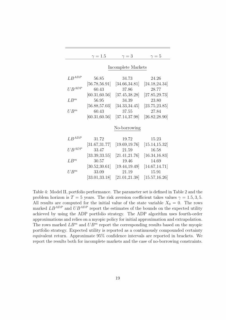
The results for Model II are summarized in Table 4. Our calibration implies a signifi-cant degree of predictability in stock returns, therefore the certainty-equivalent returns

12

achievable by the constructed portfolios are quite high. We see a clear pattern across thedifferent risk aversion values: the ADP policy outperforms the myopic policy in terms ofthe achieved expected utility, which is expressed as a lower bound on the optimal value.The difference is not large, due to the fact that expected returns on the stock index inour model are quite volatile and capturing this predictability through a myopic policyseems to have a first-order affect on expected utility. Moreover, the variable predictingstock returns is not well hedged by any of the risky assets, diminishing the importanceof the hedging component of demand. It is interesting that the upper bound obtainedfrom the ADP policy is not always superior to the one based on the myopic policy.This must be due to the fact that to evaluate the upper bound one must approximatethe partial derivatives of the value function with respect to the state variables. If suchapproximation turns out to be inaccurate, one can obtain tighter bounds by using themyopic strategy and simply setting the above partial derivatives to zero.

6 Conclusion

As our results indicate, the ADP algorithm is a viable tool for solving practically inter-esting portfolio choice problems. The method is accurate in the considered examples,whether the myopic policy is close to optimality or not. As our numerical experimentsdemonstrate, the accuracy of the ADP-based approximate solutions can be reliablygauged by the duality-based simulation method of HKW. Together, the two algorithmsform a powerful set of tools which can be used to tackle difficult, high-dimensionalproblems.

13

Barberis, N. 2002. Investing for the Long Run When Returns are Predictable. Journalof Finance. 55 225-264.

Brandt, M., A. Goyal, P. Santa-Clara, and R. Stroud. 2005. A Simulation Approachto Dynamic Portfolio Choice with an Application to Learning About Return Pre-dictability. Review of Financial Studies 18, 831-873.

Brennan, M. and Y. Xia. 2002. Dynamic Asset Allocation Under Inflation. Journal ofFinance. 57 1201-1238.

Brennan, M., E. Schwartz, and R. Lagnado. 1997. Strategic Asset Allocation. Journalof Economic Dynamics and Control. 21 1377-1403.

Campbell, J. and L. Viceira. 1999. Consumption and Portfolio Decisions When Ex-pected Returns are Time Varying. The Quarterly Journal of Economics. 114433-495.

Campbell, J. and L. Viceira. 2002. Strategic Asset Allocation – Portfolio Choice forLong-Term Investors. Oxford University Press, USA.

Campbell, J., Y. Chan and L. Viceira. 2003. A Multivariate Model of Strategic AssetAllocation. Journal of Financial Economics. 67 41-80.

Chacko, G. and L. Viceira. 2005. Dynamic Consumption and Portfolio Choice withStochastic Volatility in Incomplete Markets. Review of Financial Studies. 181369-1402.

Cox, J. and C.F. Huang. 1989. Optimal Consumption and Portfolio Policies WhenAsset Prices Follow a Diffusion Process. Journal of Economic Theory. 49 33-83.

Duffie, D. 2001. Dynamic Asset Pricing Theory . 3rd ed. Princeton University Press,USA.

Haugh, M., L. Kogan and J. Wang. 2006. Portfolio Evaluation: A Duality Approach.Forthcoming, Operations Research.

Karatzas, I., J. Lehoczky, S. Sethi and S. Shreve. 1986. Explicit Solution of a GeneralConsumption/Investment Problem. Mathematics of Operationas Research. 11261-294.

Kim, T. and E. Omberg. 1986. Dynamic Nonmyopic Portfolio Behavior. Review ofFinancial Studies. 9 141-61.

Merton, R. 1971. Optimum Consumption and Portfolio Rules in a Continuous-TimeModel, Journal of Economic Theory 3, 373-413.

Merton, R. 1990. Continuous-Time Finance. New York: Basil Blackwell.

14

Munk, C. 2000. Optimal Consumption/Investment Policies with Undiversifiable In-come Risk and Liquidity Constraints. Journal of Economic Dynamics and Control.24 1315-1343.

Liu, J. 1998. Dynamic Portfolio Choice and Risk Aversion. Working paper. StanfordUniversity, Palo Alto.

Longstaff, F. and E. Schwartz. 2001. Valuing American Options by Simulation: ASimple Least-Squares Approach. Review of Financial Studies 14 113-147.

Tsitsiklis, J., and B. Van Roy. 2001. Regression Methods for Pricing Complex American–Style Options. IEEE Transactions on Neural Networks 12 694-703.

Wachter, J. 2002. Portfolio and Consumption Decisions under Mean-Reverting Re-turns: An Exact Solution for Complete Markets. Journal of Financial and Quan-titative Analysis 37 63-91.

Wachter, J. 2003. Risk Aversion and Allocation to Long-Term Bonds. Journal ofEconomic Theory 112 325-333.

Wachter, J. and A. Sangvinatsos. 2005. Does the Failure of the Expectations Hypoth-esis Matter for Long-Term Investors?, Journal of Finance 60 179-230.

15

Parameter Values

K 0.5760 0 00 3.3430 0

-0.4210 0 0.0830

σX 1.0000 0 00 1.0000 00 0 1.0000

δ0 0.0560

δ1 0.0180 0.0070 0.010

λ>1 0 0 0

λ2 0 0 00 0 00 0 0

Table 1: Model I, calibrated parameters. The market consists of the risk-free asset anda long-term bond. The data-generating process is Gaussian. See Section 5.1 for details.

16

Parameter Values

K 0.5760 0 0 00 3.3430 0 0

-0.4210 0 0.0830 00 0 0 0.0800

σX 1.0000 0 0 0 00 1.0000 0 0 00 0 1.0000 0 00 0 0 -0.1985 0.3473

σS -0.0126 0.0057 -0.0295 0.0143 0.000

δ0 0.0560

δ1 0.0180 0.0070 0.0100 0

λ>1 -0.5630 -0.2450 -0.2190 0.4400 0

λ2 0 1.7540 0 00 -1.8150 0 0

0.5370 0.3760 -0.0820 00.1110 0.3050 -0.0170 0.200

0 0 0 0

Table 2: Model II, calibrated parameters. The market consists of the risk-free asset,two long-term bonds, and a stock index. Stock returns are predictable and the processfor the predictive variable is independent of the processes driving the term structure ofinterest rates. The data-generating process is Gaussian. See Section 5.1 for details.

17

Incomplete Markets

LBADP 5.22[5.22,5.23]

UBADP 5.53[5.53,5.54]

LBm 4.42[4.41,4.42]

UBm 5.59[5.58,5.60]

LBLT 5.51[5.51,5.51]

UBLT 5.53[5.52,5.53]

No-borrowing

LBADP 5.29[5.28,5.29]

UBADP 5.67[5.65,5.69]

LBm 4.42[4.41,4.42]

UBm 6.87[6.80,6.94]

LBLT 5.51[5.51,5.51]

UBLT 5.58[5.57,5.59]

Table 3: Model I, portfolio performance. The parameter set is defined in Table 1 andthe problem horizon is T = 5 years. The risk aversion coefficient is γ = 15. All resultsare computed for the initial value of the state variable X0 = 0. The rows marked LBADP

and UBADP report the estimates of the bounds on the expected utility achieved by usingthe ADP portfolio strategy. The ADP algorithm uses fourth-order approximations andrelies on a myopic policy for initial approximation and extrapolation. The rows markedLBm and UBm report the corresponding results based on the myopic portfolio strategy.Expected utility is reported as a continuously compounded certainty equivalent return.Approximate 95% confidence intervals are reported in brackets. The rows marked LBLT

and UBLT report the bounds based on the policy of holding all of the portfolio in along-term bond maturing at time T . We report the results both for incomplete marketsand the case of no-borrowing constraints.

18

γ = 1.5 γ = 3 γ = 5

Incomplete Markets

LBADP 56.85 34.73 24.26[56.78,56.91] [34.66,34.81] [24.18,24.34]

UBADP 60.43 37.86 28.77[60.31,60.56] [37.45,38.28] [27.85,29.73]

LBm 56.95 34.39 23.80[56.88,57.03] [34.33,34.45] [23.75,23.85]

UBm 60.43 37.55 27.84[60.31,60.56] [37.14,37.98] [26.82,28.90]

No-borrowing

LBADP 31.72 19.72 15.23[31.67,31.77] [19.69,19.76] [15.14,15.32]

UBADP 33.47 21.59 16.58[33.39,33.55] [21.41,21.76] [16.34,16.83]

LBm 30.57 19.46 14.69[30.52,30.61] [19.44,19.49] [14.67,14.71]

UBm 33.09 21.19 15.91[33.01,33.18] [21.01,21.38] [15.57,16.26]

Table 4: Model II, portfolio performance. The parameter set is defined in Table 2 and theproblem horizon is T = 5 years. The risk aversion coefficient takes values γ = 1.5, 3, 5.All results are computed for the initial value of the state variable X0 = 0. The rowsmarked LBADP and UBADP report the estimates of the bounds on the expected utilityachieved by using the ADP portfolio strategy. The ADP algorithm uses fourth-orderapproximations and relies on a myopic policy for initial approximation and extrapolation.The rows marked LBm and UBm report the corresponding results based on the myopicportfolio strategy. Expected utility is reported as a continuously compounded certaintyequivalent return. Approximate 95% confidence intervals are reported in brackets. Wereport the results both for incomplete markets and the case of no-borrowing constraints.

19

A Upper bound on expected utility: a quadratic

subproblem

In this section we derive explicit solutions to constrained quadratic optimization prob-lems involved in estimating an upper bound on the optimal expected utility. See HKWfor a general formulation and definitions related to the dual formulation. We considerhere the case of incomplete markets and no-borrowing constraints.

We start with a simpler case of Model I. The quadratic programming problem that needsto be solved repeatedly during Monte Carlo simulations is

min1

2||Λ− Λν ||2

s.t σ1Λν = σ1Λ + ν

ν is feasible

Above, Λ is the candidate for a market price of risk in a fictitious market, obtainedfrom an approximate value function produced by the ADP algorithm (see HKW for

definitions). Λν is the market price of risk in a fictitious complete market, which we useto compute an upper bound on the expected utility. ν is a scalar in this case, whichparameterizes feasible fictitious markets.

When markets are incomplete, the only feasible value of ν is zero. We are thus facedwith a simple projection problem,

min1

2||Λ− Λν ||2

s.t σ1(Λν − Λ) = 0

which has an explicit solution:

Λν = Λ−[(σ1σ

>1 )−1σ1(Λ− Λ)

]σ>1 . (22)

In the case of no-borrowing constraints, the feasible set is ν ≤ 0. Therefore, we aresolving

min1

2||Λ− Λν ||2

s.t σ1(Λν − Λ) ≤ 0.

We are thus faced with two possibilities. If σ1(Λ−Λ) ≤ 0, then Λν = Λ. Otherwise, Λν

is given by (22).

20

We now consider Model II. The quadratic subproblem has a similar form. Let Σ denotethe diffusion matrix of returns on risky assets and define variables y = Λν − Λ andb = Σ(Λ− Λ). Then, the quadratic subproblem takes form

min1

2||y||2

s.t. Σy − νı = b

ν is feasible

ı is a vector of ones of the same dimension as the number of risky assets and, again, ν isa constant. When markets are incomplete, ν = 0 and the optimization problem reducesto

min1

2||y||2

s.t. Σy = b

which has the solutiony = Σ>(ΣΣ>)−1b.

In the case of no-borrowing constraints, the feasible set is given by ν ≤ 0. We are nowfacing two distinct cases. Relaxing the equality constraints with Lagrange multipliers π,we see that if the system of linear equations

y − Σ>π = 0

ı>π = 0

Σy − νı = b

has a solution with ν ≤ 0, then we have an optimal y. Otherwise, we must set ν = 0,and the optimal y is given by the solution for the case of incomplete markets.

21