Portfolio Optimization by Mean-Value at Risk Framework

Appl. Math. Inf. Sci.10, No. 5, 1935-1948 (2016) 1935

Applied Mathematics & Information SciencesAn International Journal

http://dx.doi.org/10.18576/amis/100535

Portfolio Optimization by Mean-Value at Risk Framework

Shokufeh Banihashemi1,∗, Ali Moayedi Azarpour 2 and Hamidreza Navvabpour2

1 Department of Mathematics, Faculty of Mathematics and Computer Science,, Allameh Tabataba’i University, Tehran, Iran.2 Department of Statistics, Faculty of mathematics and Computer Science, Allameh Tabataba’i University, Tehran, Iran.

Received: 20 Aug 2015, Revised: 21 Dec 2015, Accepted: 24 Dec2015Published online: 1 Sep. 2016

Abstract: The purpose of this study is to evaluate various tools used for improving performance of portfolios and assets selectionusingmean-value at risk models. The study is mainly based on a non-parametric efficiency analysis tool, namely Data Envelopment Analysis(DEA). Conventional DEA models assume non-negative valuesfor inputs and outputs, but variance is the only variable in models thattakes non-negative values. At the beginning variance was considered as a risk measure. However, both theories and practices indicatethat variance is not a good measure of risk and has some disadvantages. This paper focuses on the evaluation process of theportfoliosand replaces variance by value at risk (VaR) and tries to decrease it in a mean-value at risk framework with negative data by usingmean-value at risk efficiency (MVE) model and multi objective mean-value at risk (MOMV) model. Finally, a numerical example withhistorical and Monte Carlo simulations is conducted to calculate value at risk and determine extreme efficiencies that can be obtainedby mean-value at risk framework.

Keywords: Portfolio, Data Envelopment Analysis, Value at Risk, Efficiency, Negative data, Mean-Value at Risk Efficiency, MultiObjective Mean-Value at Risk

1 Introduction

For investors, best portfolios or assets selection and risksmanagement are always challenging topics. Investorstypically try to find portfolios or assets offering less riskand more return. Markowitz [18] works are the first typeof these kinds of attempts to find such securities in amathematical way. The model he introduced, known asMarkowitz or mean-variance (MV) model, tries todecrease variance as a risk parameter in all levels ofmean. This model results in an area with a frontier calledefficient frontier. Morey and Morey [21] proposedmean-variance framework based on Data EnvelopmentAnalysis, in which variances of the portfolios are used asinputs and expected return are used as outputs to DEAmodels. Data Envelopment Analysis has proved theefficiency for assessing the relative efficiency of DecisionMaking Units (DMUs) that employs multiple inputs toproduce multiple outputs (Charnes et al. [8]). Briec et al.[5] tried to project points in a preferred direction onefficient frontier and evaluate points efficiencies by theirdistances. Demonstrated model by Briec et al. [6], whichis also known as a shortage function, has someadvantages. For example optimization can be done in any

direction of a mean-variance space according to theinvestors ideal. Such as, in shortage function, efficiencyof each security is defined as the distance between theasset and its projection in a pre-assumed direction. As aninstance, in variance direction, efficiency is equal to theratio between variance of projection point and variance ofasset. Based on this definition if distance equals to zero,that security is on the frontier area and its efficiencyequals to 1. This number, in fact, is the result of shortagefunction which tries to summarize value of efficiency by anumber. Similar to any other model, mean-variancemodel has some basic assumptions. Normality is one ofits important assumptions. In mean-variance models,distributions of means of securities on a particular timehorizon should be normal. In contrast Mandelbrot [17]showed, not only empirical distributions of means arewidely skewed, but they also have thicker tails thannormal. Ariditti [1] and Kraus and Litzenberger [16] alsoshowed that expected return in respect of third moment ispositive. Ariditti [1],Kane [14], Ho and Cheung [11]showed that most investors prefer positive skewed assetsor portfolios, which means that skewness is an outputparameter and same as mean or expected return, shouldbe increased. Based on Mitton and Vorkink [20] most

∗ Corresponding author e-mail:[email protected]

c© 2016 NSPNatural Sciences Publishing Cor.

http://dx.doi.org/10.18576/amis/100535

1936 Sh. Banihashemi et al.: Portfolio Optimization by Mean-Value at Risk Framework

investors scarify mean-variance model efficiencies forhigher skewed portfolios. In this way Joro and Na [13]introduced mean-variance-skewness framework, in whichskewnesses of returns considered as outputs.However, intheir recommended model same as mean-variance model,optimization is done in one direction at a time. Briec et al.[6] introduced a new shortage function which obtains anefficiency measure looks to improve both mean andskewness and decreases variance at a time. Kerstens et al.[15] introduced a geometric representation of the MVSfrontier related to new tools introduced in their paper. Inthe new models instead of estimating the whole efficientfrontier, only the projection points of the assets arecomputed. In these models a non-linear DEA-typeframework is used where the correlation structure amongthe units is taken into account. Nowadays, most investorsthink consideration of skewness and kurtosis in modelsare critical. Mhiri and Prigent [19] analyzed the portfoliooptimization problem by introducing higher moments ofreturn - the main financial index. However, using thisapproach needs variety of assumptions hold. Therefore,there is not a general willingness to incorporate higherorder moments. Up to this point the assumption is thatvariance is a parameter that evaluates risk and it ispreferred to be decreased, although, not everybody wantsthis. For example a venture capitalist prefers riskyportfolios or assets, followed by more return than normal.In mean-variance models evaluation, such situations areconsidered as undesirable. But they are not reallyundesirable for those who are interested in risk for higherreturns. There are some approaches, trying to addresssuch ambiguities by introducing other parameters, such assemi variance. However, each approach has its owndisadvantage which makes it less desirable. A newapproach to manage and control risk is value at risk(VaR). This new approach focuses on the left hand side ofthe range of normal distribution where negative returnscome with high risk. Value at risk was first proposed byBaumol [3]. The goal is to measure loss of return on leftside of the portfolios return distribution by reporting anumber. Based on VaR definition, it is assumed thatsecurities have a multivariate normal distribution;however, they are also true for non-normal securities.Silvapulle and Granger [27] estimated VaR by usingordered statistics and nonparametric kernel estimation ofdensity function. Chen and Tang [9] investigated anothernonparametric estimation of VaR for dependent financialreturns. Bingham et al. [4] studied VaR by usingsemi-parametric estimation of VaR based on normalmean-variance mixtures framework. A fullynonparametric estimation of dynamic VaR is alsodeveloped by Jeong and Kang [12] based on the adaptivevolatility estimation and the nonparametric quantilesestimation. Angelidis and Benos [2] calculated VaR forGreek Stocks by employing nonparametric methods, suchas historical and filtered historical simulation. Recently,the nonparametric quantile regression, along with theextreme value theory, is applied by Schaumburg [24] to

predict VaR. All together Using VaR as a risk controllingparameter is the same as variance; a similar framework isapplied: variance is replaced by VaR and then it isdecreased in a mean-VaR space. In this study value at riskis decreased in a mean-value at risk framework withnegative data. Conventional DEA models, as used byMorey and Morey [21], assume non-negative values forinputs and outputs. These models cannot be used for thecase in which DMUs include both negative and positiveinputs and/or outputs. Poltera et al. [23] consider a DEAmodel which can be applied in cases where input/outputdata take positive and negative values. Models which aregoing to be introduced in this paper are developed basedon this model; although, there are also other models canbe used for negative data such as Modified slacks-basedmeasure model (MSBM), Sharpe et.al. [25],semi-oriented radial measure (SORM), Emrouznejad[10]. The paper is organized as follows. Section 2presents a quick look at DEA models, mean-variancemodels of Markowitz [18], Morey and Morey [21], Joroand Na [13], and Shortage function. In section 3Variance-covariance method, historical and Monte Carlosimulation methods, for calculating VaR, are brieflyreviewed. In section 4 mean-VaR models are developedby using historical and Monte Carlo simulation methodswith negative data. Section 5 represents a real globalapplication and proposed models are applied to evaluateportfolios performance. And finally in section 6 acomparison between models is made.

2 Background

First portfolio theory for investing was published byMarkowitz [18]. Markowitz approach begins withassuming that an investor has given money to invest at thepresent time and this money will be invested for aninvestors preferred time horizon. At the end of theinvesting period, the investor will sell all of the assets thatwere bought at the beginning and then either expenses orreinvests that money. Since portfolio is a collection ofassets, it is better to select an optimal portfolio from a setof possible portfolios. Hence, the investor shouldrecognize returns of portfolios’ assets (or portfolios’return) and their standard deviations. This means that theinvestor wants to maximize expected return and minimizeuncertainty (risk). Rate of return (or simply return) of theinvestors wealth from beginning to the end of period iscalculated as follows:

Return=

(end of period wealth)− (beginning of period wealth)beginning of period wealth

(1)or


Appl. Math. Inf. Sci.10, No. 5, 1935-1948 (2016) /www.naturalspublishing.com/Journals.asp 1937

Return=

log(end of period wealth)− log(beginning of period wealth).(2)

Since Portfolio is a collection of assets, its return (rP) canbe calculated in a similar manner. Thus according toMarkowitz [18], the investor should consider rates ofreturns associated with any of these portfolios as, what iscalled in statistics, a random variable. These variables canbe described by mean(rP) and standard deviation(σP),which are calculated as follows:

r̄P =n

∑i=1

λir̄i, (3)

σP = [n

∑i=1

n

∑j=1

λiλ jωi j]12 (4)

where n is the number of assets in the portfolio,ri isexpected return of asseti calculated from equation1 or 2and rP is expected return of portfolio. Also,λi isproportion of portfolios initial value invested in assetiandσP is standard deviation of portfolio, andωi j showsmatrix of covariance of returns between assetsi and j. Sooptimal portfolio from a set of portfolios either offeringmaximum expected return among a varying levels of riskor minimum risk for a varying levels of expected returns(Sharpe [26]).

Based on Markowitz [18] theory, it is required tocharacterize the whole efficient frontier, which for largenumber of assets is cumbersome. In contrast Morey andMorey [21] measured efficiency of under evaluationassets through DEA models. Data envelopment analysis(DEA) is a nonparametric method for evaluating theefficiency of systems with multiple inputs or outputs. Inthis section we present, not discussing in details, somebasic definitions, models and concepts that will be used inother sections. ConsiderDMU j ( j = 1, · · · ,n) where eachDMU consumes m inputs to produce s outputs. Also,suppose that the observed input and output vectors ofDMU j are X j = (x1 j, · · · ,xm j) and Yj = (y1 j, · · · ,ys j)respectively, and letX j ≥ 0, X j 6= 0 andYj ≥ 0, Yj 6= 0. Abasic DEA formulation in input orientation is as follows:

min θ − ε(∑sr=1 s+r +∑m

i=1s−i )s.t. ∑n

j=1λ jxi j + s−i = θxio i = 1, · · · ,m,

∑nj=1λ jyr j − s+r = yro r = 1, · · · ,s,

λ ∈ Λ ,s+,s− ≥ 0, ε ≥ 0

(5)

whereλ is a n-vector of variablesλi, s+ is a s-vector ofoutput slacks,s− is a m-vector of input slacks,ε is a non-Archimedes factor, and the setΛ is defined as follows:

λ =

λ ∈ Rn+

with constant returns to scale,λ ∈ Rn

+, 1T λ ≤ 1with non-increasing returns to scale,

λ ∈ Rn+, 1T λ = 1

with variable returns to scale.

Note that subscripto refers to the under evaluation unit. ADMU is efficient if and only if θ = 1 and all slackvariables (s+ and s−) are equal to zero otherwise it isinefficient, (Charnes et al. [8]). In the DEA formulation(5) , the left-hand-sides of constraints define an efficientunit, while, the scalars in the right-hand sides are theinputs and outputs of the under evaluation unit and thetheta is a multiplier that defines the distance from theefficient frontier. The slack variables are also used toensure that the efficient points are fully efficient. Insolving DEA models three different attitudes can beconsidered. DEA models can be input, output orcombined oriented, where, each orientation has its owninterpretation in financial fields.

Fig. 1: Different projections (input oriented, output oriented andcombined oriented).

Figure1 illustrates different projections’ orientationswhich are consist of input, output and combined orientedin DEA models. C is the projection point obtained byfixing level of expected return as output and minimizingvariance (input oriented); B is the projection pointobtaining by maximizing output (return) and minimizinginput (variance) simultaneously (combined oriented), andD is the projection point obtaining by fixing variance(input) level and maximizing return (output oriented).

In recent years these models have been widely used toevaluate portfolios’ efficiencies. Morey and Morey [21]used DEA model to measure efficiency of underevaluation assets only by characterizing projection points.Based on DEA model, efficiency of an assetθ is thedistance between an asset and its projection. In fact,efficiency is the ratio between the variance of theprojection points and the variance of the under evaluationassets. In Morey and Morey [21] framework, there are nassets, andλ j is the weight of assetj in the projectionpoint. r j is the expected return of assetj. s1 is a s-vectorof output slacks ands2 is a m-vector of input slacks. Also,ε is a non-Archimedes factor andµo andσ2

o are expectedreturn and variance of under evaluation asset respectively.


www.naturalspublishing.com/Journals.asp


Efficiency measure (θ ) can be determined by followingmodel,

min θ − ε(s1+ s2)s.t. E(∑n

j=1λ jr j)− s1 = µo

E[(∑nj=1λ j(r j − µ j))

2]+ s2 = θσ2o ,

∑nj=1λ j ≤ 1 ∀λ≥ 0.

(6)

Model 6 is developed based on the non-parametricefficiency analysis named Data Envelopment Analysis.Briec et al. [6] used directions in optimization. They triedto project the under evaluation assets on the efficientfrontier via maximizing return and minimizing variancesimultaneously in the direction of the vectorg = (|µo|,−|δ 2

o |) using the following model:

max βs.t. E(∑n

j=1 λ jr j)≥ µo +β µo

var[r(λ)]≤ σ2o −β σ2

o ,∑n

j=1 λ j ≤ 1 ∀λ≥ 0.(7)

where

var[r(λ)] = E[(r(λ)−E[r(λ)])2] =n

∑i, j=1

λiλ jωi j. (8)

When model7 equals zero, the under evaluation unit is onthe efficient frontier. In equation8 n is number of assetsin the portfolio.λ j is proportion of portfolios initial valueinvested in assetj andλ is a n-vector of variablesλ j.Also r j is return of assetj andωi j is covariance of returnsbetween asseti and assetj.

Later studies revealed that skewness is a preferredmoment by investors. Based on studies of Mandelbrot[17], Ariditti [ 1], Kane [14] and Ho and Cheung [11],investors try to choose assets with higher rates ofskewness. Therefore, Joro and Na [13] extended model6into mean-variance-skewness model whereκo is theskewness of the under evaluation asset. The followingmodel measures efficiency (θ ) of the under evaluationasset.

minθ −ε(s1+ s2+ s3)s.t. E[∑n

j=1λ jr j]− s1 = µo

E[(∑nj=1 λ j(r j − µ j))

2]+ s2 = θσ2o ,

E[(∑nj=1 λ j(r j − µ j))

3] = κo,

∑nj=1 λ j ≤ 1, ∀λ ≥ 0.

(9)

Model 9 projects the asset on the efficient frontier byfixing expected return and skewness levels andminimizing variance.

In the conventional DEA models, eachDMU j( j = 1, · · · ,n) is specified by a pair of non-negative

input and output vectors(xi,y j) ∈ R(m+s)+ , in which inputs

xi j (i = 1, · · · ,m) are utilized to produce outputs,yr j (r = 1, · · · ,s). These models cannot be used for the

cases in which DMUs include both negative and positiveinputs and/or outputs. Portela et al. [23] considered aDEA model which can be applied in cases whereinput/output data take both positive and negative values.Range Directional Measure (RDM) model proposed byPortela et al. [23] is as follow:

maxβs.t. ∑n

j=1 λ jxi j ≤ xio +β Rio i = 1, · · · ,m,

∑nj=1 λ jyr j >= yro −β Rro r = 1, · · · ,s,

∑nj=1 λ j = 1, j = 1, · · · ,n.

(10)

where

Rio = xio −minj{xi j : j = 1, · · · ,n}, i = 1, · · · ,m,

(11)

Rro = maxj{yr j : j = 1, · · · ,n}− yro, r = 1, · · · ,s.

(12)

Ideal point(I) within the presence of negative data, is

I = (max j{yr j : r = 1, · · · ,s},minj{xi j : i = 1, · · · ,m}),

(13)and the goal is to project each under evaluation assets’points to this ideal point. Other models that use negativedata are modified slacks-based measure model (MSBM),Emrouznejad [10] and semi-oriented radial measure(SORM), Sharpe et al. [25].

2.1 Value at risk

Value at Risk (VaR) is defined as maximum amount ofinvest that one may loss in a specified time interval.Calculation of VaR can be done through differentmethods. In this paper variance-covariance method,historical and Monte Carlo simulations are introduced.Each method has one or more assumptions. As aninstance, Variance-covariance method can be used onlywhen assets’ returns are normally distributed; therefore,before normality check should be performed. In contrastwith variance-covariance method, Historical simulation isa distribution free method. In this method withoutsearching for an exact distribution we use returns originaldistribution for future forecasting. In Monte Carlomethod, simulated data are used to findVaR. Now onemay ask about differences of these three methods. That iswhat will be reviewed in this paper. One ofVaRsadvantages is difference consideration among riskaversion investors and risk lovers followed by largerreturns; moreover, it can be calculated easily. Statistically,VaR is defined as the quantile of a distribution. That is:

p(∆Pk >−VaR) = 1−α (14)

Where ∆Pk defined asPk+1 − Pk and α is defined asconfidence leve. In this definition probability of losing



more invest thanVaR is equal to alpha (α). For example ifa specified investment is done by 100 people for a year,alpha percent of investors may loss more money thanVaRin one year. Based on this definition, we need a statisticaldistribution to estimate a confidence level forVaR. Butthe most challenging part is choosing of a distribution. Sosimulation is the most important step in of ourcalculations. In following sections we will go throughdifferent methods ofVaR calculation.

2.1.1 Variance-covariance method

Variance-covariance method is one of the parametricmethods that were suggested by Morgan [22]. In thismethod returns of assets should be normally distributed,and by using variance and covariance of returns,VaR iscomputed. Furthermore, time interval is usually taken as aday. Consequently, average return of each day is aroundzero. Consider return of a portfolio through a 200 dayshorizon equals to 20% then return of each day is about0.001 percent. As mentioned earlier, this model is basedon this assumption that returns of assets are assumed tofollow conditional normal distribution;although, returnofassets by themselves may not normally distributedbecause of outliers existence (distributions with fat tails).Adapting of variance-covariance method means one hasaccepted normal distribution assumption, then variancesand covariances can easily be estimated andVaR can becomputed. Drawbacks of this approach are,

–Wrong distribution assumption, if returns distributionsare not really normally distributed;

–Input error, whenever a parameter is estimated, itfollowed by an error; and

–Non-stationary variables, when returns of our assetsare gathered over time. So variances and covariancesacross assets might change.

Some works should be done to provide approaches fordealing with these weaknesses. Among these approaches,sampling and time series methods are suggested, forexample. In many situations we may not knowdistributions and it may also be impossible to obtainthem, in such cases one may use one of the othermethods.

2.1.2 Historical simulation

Historical simulation is a non-parametric method inwhich no specific distribution is considered; In factVaR isestimated by consideration of a hypothetical time seriesof returns and assumption that changes of future data arebased on historical changes that changes in past continuein future. Also in this approach inferences are not basedon normality assumption. The other difference of thismethod with other methods is weighting. More clearly, inthis method equal weights are assigned to each day in the

time series, and a potential problem occurs if data have atrend, means less return in farther past and more return inearlier past. Changes in historical distribution of returnsin future are also another challenging situation. Simplicityof historical simulation method raises its weaknesses.Most of approaches estimateVaR based on prior data, buthistorical method relies much more on what happened inpast. Historical data are not always reliable. Therefore,past is not all. Also as mentioned earlier data may have atrend over time. Imagine situations that data are showinga moderate but stable increase as time goes on. Inhistorical method data points are weighted equallythough, earlier data have more effect on future, so shouldhave more weights. Furthermore, historical approach isbased on what we had in the past. Since for new assets nohistorical data are available, values at risk cannot beestimated. To overcome these weaknesses, new methodssuch as weighting recent past data more and combinationof time series method with historical simulation can beused.

2.1.3 Monte Carlo simulation

This method is based on stronger assumptions aboutdistribution of returns in comparison with historicalsimulation method. In this method probability distributionof returns should be specified. Once distribution isspecified, many samples of returns are simulated andparameters are computed based on those samples.Difficulties of Monte Carlo simulation are in two levels.First, for portfolios having many assets, many probabilitydistributions should be specified. Second, for each assetwhen its distribution is established, simulation should bedone many times. Bulk of computations in Monte Carlosimulation method is its main weakness point. Thats whymany users prefer historical simulation.

2.1.4 Comparing approaches

Each of these approaches has advantages anddisadvantages. Variance-covariance method is goodapproach when the distribution of returns is normal. Ifthis assumption is not held, this method may result inmisleading values. However, when our data are gatheredover a short time interval, a week for example, thismethod can be reliable. Historical simulation approach isgood since no assumption is made for probabilitydistribution of data and this method results in reliablevalues assuming distribution stability of returns over time.Monte Carlo method does its best in longer time periods,where historical data is not station and normalityassumption is not held.




3 Proposed models in mean-value at riskframework

In this section, bases of Mean-VaR model andfoundations to compute efficient frontier is provided. Ourmethod is based on Rang Directional Measure (RDM)model proposed by Portela et al. [23] and multi objectiveoptimization models. Mean-Value at Risk models try tomaximize proportional reduction in VaR dimension, as arisk measure, while maximizing mean in the sameproportion. That proportion is efficiency of underevaluation portfolio. This section summarizes essentialdefinition of mean-VaR models and their framework. Firstof all some definitions are developed. Assume a portfoliois going to be selected from n financial assets. If we showproportion of invested money in asset j withλ j, aportfolio is a vector proportions (λ ) of each n assets.While no short sales are considered sum of proportionsequals 1 (∑n

j=1 λ j = 1). It is also obvious that allproportions are equal or greater than zero for allj ∈ {1, · · · ,n} and the set of our admissible portfolios iswritten as:

φ = {λ j ∈ Rn;

n

∑j=1

λ j = 1,λ j ≥ 0} (15)

Return of portfolio,r(λ ), is defined as:

r(λ ) =n

∑j=1

λ jr j (16)

Expected return of this portfolio is straightforwardlycomputed as:

E(r(λ )) =n

∑j=1

λ jE(r j) (17)

Three methods to compute Value at risk of an asset wasmentioned in Section 3. Frameworks remain unchangedfor portfolios. From any preferred method,VaR iscalculated based on returns. To compute VaR, expectedreturns of under evaluation portfolio over a specified timeinterval should be gathered.

We definef : φ → R2 as:

f (λ) = (E[r(λ)],VaR[r(λ)] (18)

Which represents expected return andVaR of a givenportfolio λ . Consequently, expected returns andVaRsprovide a two-dimensional space and a point inR2 spacewhich is called aMVaR point. Based on defined functiondisposable set is:

f (φ) = { f (λ);λ ∈ φ}. (19)

Here same as mean variance model, in order to get aconvex set, disposal region can be extended in thefollowing way:

DR = f (φ)+ (R−×R+). (20)

Mean-VaR models evaluate efficiency through distance ofMVaR points to the efficient frontier. Same as othermodels two types of frontiers exist.

Definition 1 Weakly efficient frontier also known astheoretical frontier defines as:

∆ w(φ) = {(µ ,VaR) ∈ DR;(−µ ′,VaR′)< (−µ ,VaR)⇒ (µ ′,VaR′) /∈ DR}

(21)This frontier is a part of the boundary of the disposal

region set. Also this disposal representation set is itselfanextension of the mean-VaR region in order to make itconvex (including imaginary portfolios). Consequently,the theoretical frontier can contain points that are notreachable by real portfolios. Naturally, strongly efficientfrontier defines as follows.

Definition 2 Strongly efficient frontier defines as:

∆ s(φ) = {(µ ,VaR) ∈ DR;(−µ ′,VaR′)≤ (−µ ,VaR) and (−µ ′,VaR′) 6= (−µ ,VaR)

⇒ (µ ′,VaR′) /∈ DR}(22)

In definitions 1 and 2µ andVaR are mean and Value atRisk (VaR) of a point in disposal region respectively.µ ′

andVaR′ are also mean and value at risk of an arbitrarypoint in Mean-VaR space. Strongly efficient frontiercontains all points that are dominated in two dimensionalmean-VaR space. But in weakly efficient frontier a pointon the frontier may dominated in at least one of twodimensions. Based on this definition, strongly efficientfrontier is contained in the weakly efficient frontier(Figure2).

Fig. 2: Presentation of strongly and weakly efficient frontier.Green line shows weakly efficient frontier, while projectionpoints on this part of frontier have positive slack variables. Lightblue line represents strongly efficient frontier. Projection pointson this part of frontier are not dominated in any dimension andall of slack variables are zero.



As can be seen in figure2 slacks variables showminimum amount that should be added to or subtractedfrom a points inputs (mean) or outputs (value at risk)respectively, in order to transfers projection point to thefirst position where it is not dominated by any otherpoints (point M*).

Definition 3 Based on model10 provided by Portela etal. [23] we propose mean-VaR models can be written asmean-VaR efficiency (MVE) model and multi objectivemean-VaR (MOMV) model. Let

g = (Rµo ,RVaRo) ∈ R+×R− and R 6= 0

be a vector shows direction in whichβ is going to bemaximized. MVE function defines as:

ξ : R2 → (0,1],ξ (y) = sup{β ;y+β g ∈ DR‖β ∈R+}.

Based on vectorg, definition and mentioned set ofβ , itis obvious that the aim is to simultaneously increasereturn and reduce Value at Risk of a portfolio in directionof vectorg. This function also cares about fundamentalconditions of global optimization on non-convex sets.One should cares about directions in interpretation ofmodels while directions affect result of MVE function.For instance proportional interpretation is suitable, ifvector of direction is chosen as

g = ((maxj (µ j)− µo),(VaRo −min(VaR j)))= (Rµo ,RVaRo). j = 1, · · · ,n

Definition 4 Let define g separately in each direction; i.e.,

g = (Rµo ,RVaRo) ∈ [0,+∞)× [0,+∞). (23)

For an under evaluation assety = (µo,VaRo) and aspecified directiong = (Rµo ,RVaRo), based on model10,the MVE function can be obtained through solving thefollowing linear model:

maxβs.t. E[r(λ)]≥ µo +β Rµo ,

VaR[r(λ)]≤VaRo +β RVaRo,∑n

j=1 λ j = 1,β ≥ 0, 0≤ λ j ≤ 1 f or j ∈ {1, · · · ,n}.

(24)

Computation on MVE function is done based on RDMmodels. When this MVE function equals zero, mean-VaRpoint is on the weakly efficient frontier. Otherwise,0 < β < 1 indicates that mean and Value at Risk of anasset should be changed in order to result in an efficientpoint on the efficient frontier (amount of inefficiency). Onthe other hand, 1− β is amount of efficiency. Asmentioned earlier strongly efficient frontier is part ofweakly efficient frontier. In such situations in order to findout projected point on which frontier is, slacks andsurpluses variables are useful. Existence of slack orsurplus variables in an optimum point shows that MVE

function resulted in a point on the weakly efficientfrontier. Means efficiency measure of under evaluationpoint is biased. This bias underestimates gains in return(mean) and reductions in risk (Value at Risk). This is theway that is used to distinguish between weakly efficientfrontier and efficient frontier which is attainable inpractice.

By using multi objective functions, the followingfunction known as multi objective mean-VaR (MOMV)model, can be defined.

Definition 5 MOMV function in direction of vectorg isdefined as:

MF : R2 → (0,1]MF(y) = sup{ 1

2 ∑i βi;µ +βg ∈ DR}.This function tries to maximizeβ in directions of

mean andVaR separately. Because of having more thanone parameter to maximize, based on rules ofoptimization of multi objective functions, average ofobjects is tried to be maximized. Note thatβ andg areboth vectors. This function evaluates arithmetic averageproportional changes in each direction, which makesinterpretations more complicated. Also note that MVEfunction might project an under evaluation asset onweakly efficient frontier while MOMV function surlyprojects on strongly efficient frontier.

MOMV function is computed through followingmodel. Consider a vectorg = (Rµo ,RVaRo) and an underevaluation asset represented byy = (µo,VaRo) inMean-VaR space.

max 12(β1+β2)

s.t. E[r(λ)]≥ µo +β1Rµo ,VaR[r(λ )]≤VaRo +β2RVaRo ,∑n

j=1 λ j = 1,β1,β2 ≥ 0, 0≤ λ j ≤ 1, f or j ∈ {1, · · · ,n}.

(25)

If this model equals zero, in contrast with MVE model,under evaluation point is on the strongly efficient frontier.On the other hand ifβi doesnt equals zero, eachβi showsproportional changes in mean and value at riskrespectfully. As a result because projection in eachdirection is independent of other directions, projectedpoints are for sure on the efficient frontier. Because of thisflexibility, MOMV function always results in projectionpoints having zero slacks or surpluses. As a consequence,by this model, the weakly and strongly efficient frontiersalways coincide. Also, as can be seen, using MOMVmodel leads to clustered projection points. This clusteringoccurs while MOMV model is a more flexible model thanMVE model in determination of optimal directions. It iswell-known that the multi objective models (like MOMVmodel) always result in larger or equal optimal valuesthan single objective models (like MVE model).Therefore, MOMV model efficiencies are always lessthan or equal to the MVE model efficiencies. Note that inspecial cases optimization can be done in one direction.




For example vectorg in direction of meanRo can be setto zero. So optimization is done by minimizing risk. Sameway can be used to maximize return.

4 Application in Iranian stock companies

In this section a comparison study is conducted tocompare methods introduced in previous sections. To dothis a sample of 20 corporations from Tehran stock israndomly selected. Each of these corporations can beconsidered as a portfolio. Returns of these assets over 62days have been gathered1. Also missing data overholidays estimated through spline interpolation method.Efficiency of each asset is going to be evaluated andmethods of computing efficiencies compared. Table1reports expected return and also value at risk of each asset(columns 3-9). In this table value at risks are calculatedby using historical and Monte Carlo simulation methods.As mentioned previously, in order to calculateVaR byusing Monte Carlo method, distribution of assets must beknown. Here because of mathematical difficulties toobtain distributions, sampling methods are being usedinstead. By consideration of a specific margin of error,number of required samples to present the wholepopulation for each asset is defined and sample sizes arereported in table1 column 2. Now by using bootstrapping method, we have repeated sampling scheme formany times, for example 1000, and value at risk of eachsample is calculated. Now average of these 1000VaRs isunbiased estimate of populationVaR.

¯VaR =1

1000

1000

∑j=1

VaR j (26)

WhereVaR j is Value at Risk of samplej and ¯VaR isunbiased estimate of populations Value at Risk.

In table 2 directions, which are used in MVE andMOMV models, are provided. Note that, DEA modelwith negative data should be used, since expected returnsmight be negative. Therefore, directions are calculated byusing equations11and12.

Now based on Values at Risk in table1 and directionsin table2, and using model24, efficiency of each asset iscalculated. Results are presented in table3. As mentionedearlier, β shows amount of inefficiency. So, an asset isefficient unlessβ equals zero. Based on data in table3,asset 10 in all levels of historical and Monet Carlosimulation is efficient. However, asset 1 in higher levelsof Historical simulation and all levels of Monte Carlosimulation is efficient. For asset 1 it can be interpreted, asthe confidence level of risk increases, it gets efficient.This shows that asset 1 is suitable for investors, whodesire to invest with higher confidence on amount of riskthat they may face.

1 Time period is from 21 April to 21 June 2014.

Same data is used and efficiency of assets iscalculated by using MOMV model (25). Results areprovided in table4. Table4 reports values of inefficiency(β ). Interpretations are same as before. Based on MOMVmodel asset 10 is the efficient asset. Also same as MVEmodel in higher levels of confidence, asset 1 getsefficient. Also by comparing results of table3 and table4,it can be concluded that results of MOMV model aregenerally greater than results of MVE model. It is ageneral characteristic of multi objective models.However, general conclusion and results obtained fromMVE and MOMV models do not change. As the lastresult, table5 presents average ofβ for both MVE andMOMV model for different methods of obtaining Valueat Risk. Table5 shows that average ofβ from MOMVmodel, in all confidence levels, is higher than average ofβ from MVE model. Also, it can be inferred as theconfidence level increases value ofβ grows.

5 Geometric representations

This section goes through visualization of Mean-Value atRisk region in order to show efficient frontier and positionof under evaluation assets. In first step 10000 portfoliosmade from mentioned assets, are shown in figure3 inthree different confidence levels. In this figure portfoliosare made using values at risk calculated through historicalsimulations. Note that since portfolios are made based onnormally distributed weights,

Fig. 3: This figure shows disposable region made by 10000portfolios from assets of table1. In this figure value at risks arecalculated from historical simulation.

Figure 3 illustrates as the risk’s confidence level,increases the whole feasible region moves rightward.Therefore, as the confidence level increases, investors getsurer about the amount of risk that may face on apredefined level of return. In fact, in higher levels ofα,risk of an under evaluation asset is calculated morepreciously. Same conclusions can be made for portfoliosmade by values at risk calculated through Monte Carlo



Fig. 4: This figure shows disposable region made by 10000portfolios from assets of table1. In this figure value at risks arecalculated from Monte Carlo simulation.

Fig. 5: Under evaluation assets (light green dots) and theirprojection points (yellow dots) on efficient frontier for 90%confidence level. Point A represents asset 10 and point Bstands for asset 1. Figure shows that projection point and underevaluation point of asset 10 coincides. Therefore, asset 10iscompletely efficient. Also asset 16 (point C) is efficient at 90%confidence risk level. Efficiencies are obtained by solving MVEmodel.

Fig. 6: Under evaluation assets (light green dots) and theirprojection points (yellow dots) on efficient frontier for 95%confidence level. Point A represents asset 10 and point B standsfor asset 1. Figure shows that projection points and underevaluation points of assets 10 and 1 coincide. Therefore, assets1 and 10 are completely efficient. Efficiencies are obtained bysolving MVE model.

simulation (Figure4). They are mostly in the middle ofdisposable area. However, by using weights which areuniformly distributed, portfolios will disperse uniformly.

Now each asset can be considered as a portfolio andits performance can be evaluated. Figures5-10 showassets position in Mean-VaR region among all 10000portfolios. In these figures projection of each asset is alsoshown. These projection points are obtained via MVEmodel. In all of these figures it can be seen that asset 10 ison the efficient frontier and its projection andcorresponding point are equivalent (point A in figures5-10). This is also true for asset 1. As the risks confidencelevel increases, this asset gets efficient. On the other hand,asset 16 (point C in figure5), which is efficient at 90%confidence risk level of historical method, in higher levelsof confidence becomes inefficient. Also, in all of figures itcan be seen that all of projection points are on the bluestraight line. This line represents strongly efficientfrontier. In figures 5 red line shows weakly efficientfrontier.

Same conclusions can be made for assets evaluated byvalues at risk computed from Monet Carlo method. InFigures11-16, projection points which are obtained fromMVMO model are shown. In these figures correspondingpoints of under evaluation assets are projected mainly ontwo points. Point A represents asset 10 and point Brepresents asset 1.


Same as before, conclusions for Monte Carlosimulation are like as historical simulation. Figures14-16are made according to values at risk computed by MonteCarlo simulation. In fact, since they are efficient andβisare also defined separately in each direction, these twopoints are acting like an index for other points. Therefore,points are projected in a clustered way.




Table 1: Original data of under evaluation assetsOriginal Data

Asset Number of Value at risknumber sample Mean Historical sim. Monte Carlo sim.

90% 95% 99% 90% 95% 99%1 17 -0.00075 0.0158 0.0174 0.0217 0.0141 0.0172 0.01862 20 -0.00035 0.0287 0.0371 0.0524 0.0299 0.0375 0.04263 22 -0.00487 0.0267 0.0405 0.0642 0.0276 0.0408 0.05094 23 -0.00071 0.0348 0.0471 0.0542 0.0344 0.0439 0.04925 11 -0.00245 0.0234 0.0320 0.0480 0.0249 0.0306 0.03116 54 0.00072 0.0198 0.0269 0.0452 0.0194 0.0275 0.04487 60 -0.00323 0.0231 0.0305 0.0401 0.0231 0.0304 0.04008 49 0.00015 0.0243 0.0296 0.0439 0.0249 0.0295 0.04299 15 0.00017 0.0373 0.0421 0.0732 0.0357 0.0468 0.050510 16 0.00568 0.0200 0.0216 0.0292 0.0178 0.0219 0.023511 16 -0.00530 0.0272 0.0420 0.0729 0.0297 0.0436 0.049212 38 -0.00060 0.0299 0.0405 0.0560 0.0316 0.0408 0.053013 27 -0.00043 0.0191 0.0223 0.0503 0.0188 0.0258 0.038214 21 -0.00705 0.0476 0.0578 0.0617 0.0445 0.0539 0.058215 15 -0.00437 0.0365 0.0406 0.0465 0.0333 0.0388 0.040616 22 -0.00118 0.0140 0.0194 0.0299 0.0149 0.0191 0.023117 26 -0.00200 0.0223 0.0331 0.0355 0.0231 0.0302 0.033818 19 0.00010 0.0211 0.0294 0.0454 0.0216 0.0293 0.033919 34 0.00114 0.0198 0.0274 0.0431 0.0199 0.0261 0.037420 18 -0.00144 0.0289 0.0321 0.0378 0.0274 0.0315 0.0333

Table 2: Directions used to project points on the efficient frontierDirections

Asset Max Mean- VaR-Min VaRnumber Mean Historical sim. Monte Carlo sim.

90% 95% 99% 90% 95% 99%1 0.0064 0.0019 0 0 0 0 02 0.0060 0.0147 0.0197 0.0307 0.0158 0.0203 0.0243 0.0106 0.0127 0.0231 0.0425 0.0135 0.0236 0.03244 0.0064 0.0208 0.0297 0.0325 0.0202 0.0267 0.03075 0.0081 0.0094 0.0146 0.0263 0.0107 0.0134 0.01266 0.0050 0.0058 0.0095 0.0234 0.0053 0.0103 0.02627 0.0089 0.0091 0.0131 0.0183 0.0090 0.0132 0.02148 0.0055 0.0104 0.0122 0.0222 0.0107 0.0123 0.02439 0.0055 0.0234 0.0247 0.0514 0.0216 0.0296 0.032

10 0 0.0060 0.0042 0.0074 0.0037 0.0047 0.004911 0.0110 0.0132 0.0246 0.0512 0.0156 0.0264 0.030612 0.0063 0.0160 0.0231 0.0342 0.0174 0.0236 0.034513 0.0061 0.0051 0.0049 0.0286 0.0047 0.0086 0.019614 0.0127 0.0336 0.0404 0.0400 0.0304 0.0367 0.039615 0.0101 0.0225 0.0232 0.0248 0.0191 0.0216 0.022116 0.0069 0.0000 0.0020 0.0081 0.0007 0.0019 0.004517 0.0077 0.0083 0.0157 0.0137 0.0089 0.013 0.015218 0.0056 0.0071 0.0120 0.0237 0.0075 0.0121 0.015419 0.0045 0.0059 0.0100 0.0214 0.0058 0.0088 0.018920 0.0071 0.0149 0.0147 0.016 0.0132 0.0143 0.0148



Fig. 8: Under evaluation assets (light green dots) and theirprojection points (yellow dots) on efficient frontier for 90%confidence level. Point A represents asset 10 and point B standsfor asset 1. Figure shows that projection points and underevaluation points of assets 10 and 1 coincide. Therefore, incontrast with historical simulation in 90% confidence level,assets 1 and 10 are completely efficient. Efficiencies are obtainedby solving MVE model.


In conclusion, efficiency measures calculated viaMVE model in comparison with MOMV model aresmaller in different confidence levels. Based on MOMVmodel, efficient company on a 90% confidence level isasset number 10 for both historical and Monte Carlosimulation methods. Asset 10 is RayanSaipa Co. andasset 1 is Mellat Bank. Also, on all confidence levels allof efficiencies calculated by Monte Carlo method aresmaller than efficiencies calculated by historical method.These results show that Monte Carlo simulation methodis much more accurate than historical method.


Fig. 11: Under evaluation assets (light red dots) and theirprojection points (yellow dots) on efficient frontier for 90%confidence level. Point A represents asset 10 and point B standsfor asset 1. Figure shows that projection points and underevaluation points of assets 10 and 1 coincide. Therefore, assets1 and 10 are completely efficient. Efficiencies are obtained bysolving MVMO model.

6 Conclusions

This paper introduced a measure for portfolioperformance evaluation using mean-value at riskefficiency (MVE) model and multi objective mean-valueat risk (MOMV) model. Morey and Morey [21], Joro andNa [13] and Kerstence et al. [15] proposed models forevaluating portfolios efficiency in which DEA model wasemployed. In these models a non-linear DEA-typeframework was used in which, the correlation structureamong the units was taken into account. In these modelsvariance was considered as a risk measure. However, boththeories and practices indicate that variance is not a goodrisk measure and has disadvantages. In this paper weintroduced two models for portfolio optimizationproblem, where, most literature only consider the




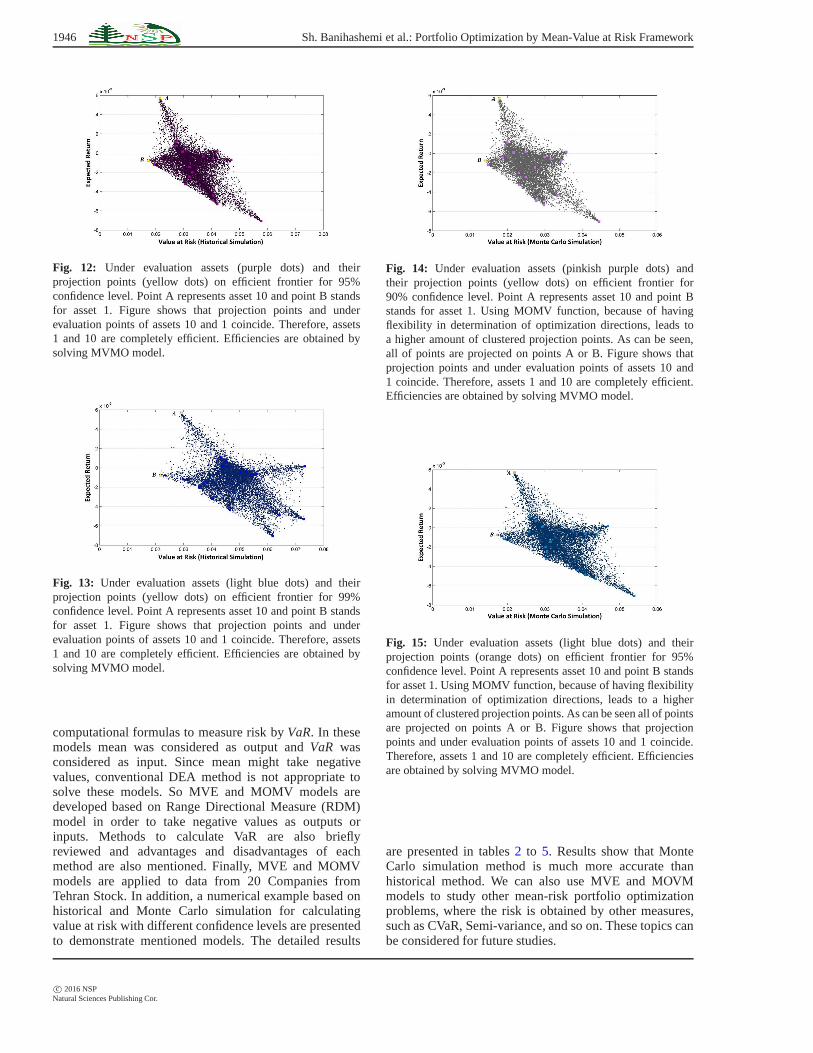
Fig. 12: Under evaluation assets (purple dots) and theirprojection points (yellow dots) on efficient frontier for 95%confidence level. Point A represents asset 10 and point B standsfor asset 1. Figure shows that projection points and underevaluation points of assets 10 and 1 coincide. Therefore, assets1 and 10 are completely efficient. Efficiencies are obtained bysolving MVMO model.

Fig. 13: Under evaluation assets (light blue dots) and theirprojection points (yellow dots) on efficient frontier for 99%confidence level. Point A represents asset 10 and point B standsfor asset 1. Figure shows that projection points and underevaluation points of assets 10 and 1 coincide. Therefore, assets1 and 10 are completely efficient. Efficiencies are obtained bysolving MVMO model.

computational formulas to measure risk byVaR. In thesemodels mean was considered as output andVaR wasconsidered as input. Since mean might take negativevalues, conventional DEA method is not appropriate tosolve these models. So MVE and MOMV models aredeveloped based on Range Directional Measure (RDM)model in order to take negative values as outputs orinputs. Methods to calculate VaR are also brieflyreviewed and advantages and disadvantages of eachmethod are also mentioned. Finally, MVE and MOMVmodels are applied to data from 20 Companies fromTehran Stock. In addition, a numerical example based onhistorical and Monte Carlo simulation for calculatingvalue at risk with different confidence levels are presentedto demonstrate mentioned models. The detailed results

Fig. 14: Under evaluation assets (pinkish purple dots) andtheir projection points (yellow dots) on efficient frontierfor90% confidence level. Point A represents asset 10 and point Bstands for asset 1. Using MOMV function, because of havingflexibility in determination of optimization directions, leads toa higher amount of clustered projection points. As can be seen,all of points are projected on points A or B. Figure shows thatprojection points and under evaluation points of assets 10 and1 coincide. Therefore, assets 1 and 10 are completely efficient.Efficiencies are obtained by solving MVMO model.

Fig. 15: Under evaluation assets (light blue dots) and theirprojection points (orange dots) on efficient frontier for 95%confidence level. Point A represents asset 10 and point B standsfor asset 1. Using MOMV function, because of having flexibilityin determination of optimization directions, leads to a higheramount of clustered projection points. As can be seen all of pointsare projected on points A or B. Figure shows that projectionpoints and under evaluation points of assets 10 and 1 coincide.Therefore, assets 1 and 10 are completely efficient. Efficienciesare obtained by solving MVMO model.

are presented in tables2 to 5. Results show that MonteCarlo simulation method is much more accurate thanhistorical method. We can also use MVE and MOVMmodels to study other mean-risk portfolio optimizationproblems, where the risk is obtained by other measures,such as CVaR, Semi-variance, and so on. These topics canbe considered for future studies.



Fig. 16: Under evaluation assets (green dots) and their projectionpoints (light green dots) on efficient frontier for 99% confidencelevel. Point A represents asset 10 and point B stands forasset 1. Using MOMV function, because of having flexibilityin determination of optimization directions, leads to a higheramount of clustered projection points. As can be seen all of pointsare projected on points A or B. Figure shows that projectionpoints and under evaluation points of assets 10 and 1 coincide.Therefore, assets 1 and 10 are completely efficient. Efficienciesare obtained by solving MVMO model.

Table 3: Efficiencies obtained by solving MVE modelEfficiencies-MVE function

Asset Historical sim. Monte Carlo sim.number 90% 95% 99% 90% 95% 99%1 0.2 0 0 0 0 02 0.7 0.82 0.8 0.81 0.81 0.833 0.73 0.86 0.86 0.81 0.85 0.884 0.77 0.88 0.81 0.85 0.85 0.865 0.64 0.79 0.79 0.76 0.76 0.746 0.41 0.67 0.74 0.55 0.66 0.847 0.65 0.78 0.74 0.74 0.76 0.838 0.61 0.74 0.74 0.73 0.71 0.839 0.79 0.85 0.87 0.85 0.86 0.86

10 0 0 0 0 0 011 0.74 0.87 0.88 0.83 0.86 0.8712 0.72 0.85 0.82 0.82 0.83 0.8713 0.43 0.53 0.79 0.55 0.64 0.814 0.87 0.91 0.86 0.9 0.9 0.915 0.81 0.86 0.8 0.85 0.84 0.8316 0 0.36 0.54 0.21 0.32 0.517 0.6 0.8 0.67 0.72 0.75 0.7718 0.5 0.73 0.75 0.65 0.71 0.7519 0.39 0.68 0.72 0.56 0.61 0.7820 0.72 0.78 0.69 0.79 0.76 0.76

Acknowledgement

The authors sincere thanks go to the known and unknownfriends and reviewers who meticulously covered the articleand provided us with valuable insights.

The authors are also grateful to the anonymousreferee for a careful checking of the details and forhelpful comments that improved this paper.

References

[1] Ariditti F. D.,1975. Skewness and investors decisions:Areply. Journal of Financial and Quantitative Analysis10,173176.

Table 4: Efficiencies obtained by solving MOMV modelEfficiencies-MOMV function

Asset Historical sim. Monte Carlo sim.number 90% 95% 99% 90% 95% 99%1 0.47 0 0 0 0 02 0.8 0.89 0.88 0.88 0.88 0.93 0.76 0.91 0.91 0.86 0.9 0.924 0.86 0.93 0.89 0.91 0.91 0.925 0.68 0.86 0.86 0.83 0.82 0.86 0.48 0.78 0.84 0.65 0.77 0.917 0.67 0.84 0.8 0.79 0.82 0.898 0.71 0.83 0.83 0.83 0.81 0.99 0.87 0.92 0.93 0.91 0.92 0.92

10 0 0 0 0 0 011 0.77 0.92 0.93 0.88 0.91 0.9212 0.81 0.91 0.89 0.89 0.9 0.9313 0.44 0.57 0.87 0.6 0.73 0.8714 0.91 0.95 0.91 0.94 0.94 0.9415 0.87 0.91 0.85 0.9 0.89 0.8916 0 0.53 0.54 0.53 0.53 0.5317 0.64 0.87 0.73 0.79 0.82 0.8418 0.58 0.83 0.84 0.75 0.81 0.8419 0.49 0.79 0.83 0.68 0.73 0.8720 0.8 0.86 0.77 0.86 0.84 0.83

Table 5: Camparison of Singel and Multi objective outputsModel Historical Simulation Monte Carlo Simulation

%90 %95 %99 %90 %95 %99Single Objective 0.56 0.69 0.69 0.65 0.67 0.73Multi Objective 0.63 0.76 0.76 0.72 0.75 0.78

[2] Angelidis T., Benos A., 2008. Value-at-Risk for Greekstocks. Multinational Finance Journal12, 67104.

[3] Baumol, W. J., 1963. An Expected Gain-Confidence LimitCriterion for Portfolio Selection. Management Science10,174182.

[4] Bingham N. H., Kiesel R., Schmidt R. ,2003. A Semi-Parametric Approach To Risk Management. QuantitativeFinance6, 426-441.

[5] Briec W., Kerstens K., Lesourd J. B., 2004. Single PeriodMarkowitz Portfolio selection, Performance Gauging andDuality: A Variation on The Luenberger shortage Function.Journal of Optimization Theory and Applications120, 127.

[6] Briec W., Kerstens K., Jokung O., 2007. Mean-Variance-Skewness Portfolio Performance Gauging: A GeneralShortage Function and Dual Approach, ManagementScience53, 135 149.

[7] Charnes A., Cooper W. W., Seiford A. Y., 1994.Data Envelopment Analysis: Theory, Methodology andApplications. Kluwer Academic Publishers, Boston.

[8] Charnes A., Cooper W. W., Rhodes E., 1978. MeasuringEfficiency of Decision Making Units, European Journal ofOperational Research2, 429444.

[9] Chen S. X., Tang C. Y., 2005. Nonparametric Inference ofValue at Risk for Dependent Financial Returns. Journal offinancial econometrics12,22755.

[10] Emrouznejad A., 2010. A Semi-Oriented Radial Measurefor Measuring The Efficiency Of Decision Making UnitsWith Negative Data, Using DEA. European journal ofOperational Research200, 297-304.

[11] Ho, Y. K., Cheung, Y. L., 1991. Behavior of Intra-DailyStock Return on an Asian Emerging Market. AppliedEconomics23, 957-966.

[12] Jeong S. O., Kang K. H.,2009. Nonparametric EstimationofValue-At-Risk. Journal of Applied Statistics10, 122538.




[13] Joro T., Na P., 2005. Portfolio Performance Evaluationin aMean-Variance-Skewness Framework. European Journal ofOperational Research175, 446461.

[14] Kane A., 1982. Skewness Preference and Portfolio Choice.Journal of Financial and Quantitative Analysis17, 1525.

[15] Kerstens K., Mounir A., Woestyne I., 2011. GeometricRepresentation of The Mean-Variance-Skewness PortfolioFrontier Based Upon The Shortage Function. EuropeanJournal of Operational Research10, 1-33.

[16] Kraus A., Litzenberger R. H., 1976. Skewness Preferenceand the Valuation of Risk Assets. Journal of Finance31,1085-1100.

[17] Mandelbrot B., 1963. The Variation of Certain SpeculativePrices. Journal of Business36, 394419.

[18] Markowitz H. M., 1952. Portfolio Selection. Journal ofFinance 7, 7791.

[19] Mhiri M., Prigent J., 2010. International PortfolioOptimization with Higher Moments. International Journalof Economics and Finance5, 157-169.

[20] Mitton T., Vorknik K., 2007. Equilibrium underDiversification and the Preference Of Skewness. Review ofFinancial Studies20, 1255-1288.

[21] Morey M. R., Morey R. C., 1999. Mutual Fund PerformanceAppraisals: A Multi-Horizon Perspective With EndogenousBenchmarking. Omega27, 241258.

[22] Morgan J. P. 1996. Risk MetricsTM: Technical Document,4th ed., NewYork: Morgan Guaranty Trust Company.

[23] Portela M. C., Thanassoulis E., Simpson G., 2004. Adirectional distance approach to deal with negative datain DEA: An application to bank branches. Journal ofOperational Research Society55, 1111-1121.

[24] Schaumburg J., 2012. Predicting Extreme Value at Risk:Nonparametric Quantile Regression with Refinements fromExtreme Value Theory. Computational Statistics and DataAnalysis56, 4081-4096.

[25] Sharpe J. A., Meng W., Liu W., 2006. A Modified Slacks-Based Measure Model for Data Envelopment Analysiswith Natural Negative Outputs and Inputs. Journal of theOperational Research Society57, 1-6.

[26] Sharpe W. F., 1985. Investment. Third Edition, Prentice-Hall.

[27] Silvapulle P., Granger C. W., 2001. Large Returns,Conditional Correlation and Portfolio Diversification: AValue-At-Risk Approach. Quantitative Finance10, 54251.

Shokufeh Banihashemiis assitant professor ofApplied Mathematicsin operational researchat Allameh Tabataba’iUniversity. Her researchinterests are in the areasof Applied Mathematics,Data Envelopment Analysis,Supply Chains, Finance. She

has published research articles in international journalsofMathematics. She is referee of mathematical andeconomics journals.

Ali MoayediAzarpour is master studentof socioeconomic statisticsat Allame Tabataba’iUniversity. He has defendedhis master thesis on portfoliooptimization. His researchinterests are in portfoliosoptimiztion and softwareprogramming. He has alsoother papers under review.

Hamidreza Navvabpouris associate professorof Statistics at AllamehTabatabai University,a selected member ofISI and managing directorof Journal of StatisticalResearch of Iran. Hisresearch interests are inareas of Survey Methodology,Sampling Methods, MissingData, Linear Models and

Multivariate Data Analysis. He has published articles inIranian and international journals.


Documents

Portfolio Optimization by Mean-Value at Risk Framework