Embed Size (px)
Citation preview
Portfolio Construction with Asymmetric Risk Measures
Harald Lohre, Union Investment, Frankfurt/Main
Thorsten Neumann, Union Investment, Frankfurt/Main
Thomas Winterfeldt, HSH Nordbank, Kiel∗
7th May 2007
Abstract
Portfolio construction techniques seek an optimal trade-off between the portfolio’s
mean return and the associated risk. Given that risk may not be properly described
by return volatility we examine alternative measures that account for the asymmetric
nature of risk, i.e. downside risk. In particular, we optimize portfolios with respect to
semideviation, semivariance, skewness, loss-oriented utility or maximum drawdown in
an empirical out-of-sample setting. To avoid bias due to misspecified return forecasts
we assume perfect foresight of returns whereas alternative risk measures are being esti-
mated from historical data. Our empirical results indicate that downside portfolio risk
is reduced for most of the investigated measures. We find significant risk reductions
for semivariance, semideviation, maximum drawdown and loss-oriented utility. How-
ever, lacking persistence both tested skewness measures are rendered rather useless for
portfolio construction purposes.
Keywords: portfolio optimization, asymmetric risk measure, skewness, maximum
drawdown, semideviation, semivariance, lower partial moments, utility function
∗Contacts: [email protected], [email protected] [email protected] (corresponding author).

1 Introduction
Since Markowitz (1952) has lifted portfolio construction to a scientific level, a number
of shortcomings of the classic mean-variance optimization approach have been discussed
controversially in literature. These are in particular the static one period character, the
high sensitivity of the optimization outcomes with respect to small changes in the inputs
and the use of volatility as a risk measure. In this paper we focus on the latter. In fact,
being a symmetric risk measure, volatility does not seem to fit most investors’ definition
of risk as the peril to end up with less than expected. Volatility counts both negative and
positive surprises as risk, not distinguishing between cold and warm rain.
Tobin (1958) was one of the first to show that volatility can only be the risk measure of
choice for quadratic utility functions or, otherwise, normally distributed returns. Both
assumptions have been proven to be unsustainable, see e.g. Mandelbrot (1963), Fama
(1965) for non-normality and Rubinstein (1973) or von Neumann and Morgenstern (1947)
for properties of utility functions. To account for the asymmetric nature of risk Roy (1952)
adds a criterion to Markowitz’ efficient frontier which selects the efficient portfolio with
the lowest probability to fall short of a given target return. Markowitz (1959) proposes
a portfolio optimization procedure based on the semivariance measure. Fishburn (1977)
employs a piecewise defined utility function model that translates downside risk depend-
ing on a risk aversion parameter and a target return. His findings indicate that investors
actually show a significant change in their risk perception below this individual threshold.
Hence, there is a broad consensus among both researchers and practitioners that asymme-
try is a reasonable property for any risk measure, what disqualifies volatility. Nonetheless,
although a number of alternatives have been proposed the mean-variance approach is still
prevalent. However, none of them has proven to be appropriate to a broad society so far.
Whatever the choice of risk measure, under perfect information an optimizer will cer-
tainly find risk-minimized portfolios for any given sample. In practice, however, portfolio
construction takes place in an ex-ante context relying on forecasts of the respective risk
measure that have to be derived from historical data. Therefore, forecastability of a risk
measure is a prerequisite in practice. This is an important challenge because risk structures
(think of correlations) are known to be unstable over time. For instance, the instability
of beta factors and, as a consequence, covariance matrices and other correlation-based
1
risk measures has been documented by numerous studies.1 Although it is important to
consider alternative risk measures in an empirical out-of-sample setting this has not been
addressed intensively in the literature. Bertsimas, Lauprete and Samarov (2004) apply a
mean-shortfall optimization procedure to empirical data, but not by means of a backtest.
Guidolin and Timmermann (2006) propose various econometric models to describe the
term structure of value at risk and expected shortfall risk measures and compare them
out-of-sample within a strategic asset allocation problem.
This paper adds to the existing evidence by empirically examining whether asymmetric
risk measures are more useful to define risk in the context of portfolio construction. To do
so, we substitute volatility as the objective function of portfolio optimization by a couple
of alternative risk measures. We compare the out-of-sample performance characteristics
of the mean variance based investment strategy to those of other risk philosophies in an
empirical backtest.
The paper is structured as follows: Section 2 introduces the alternative risk measures
considered. Section 3 covers the empirical methodology. Section 4 discusses our empirical
findings. Section 5 concludes.
2 Candidate Asymmetric Measures of Risk
All of the risk measures discussed in this section are downside risk oriented. In contrast
to symmetric risk measures they only treat negative deviations as risk but not positive
deviations.
Value-at-Risk
Given the random return R of a portfolio for a certain holding period the value at risk
(VaR) determines the loss corresponding to the lower quantile of its distribution for a given
(small) probability. Let the probability be p = 0.01, then
VaRp(R) = −F−1R (0.01)W,
where FR is the cumulative distribution function of R and W is the investor’s initial wealth,
a constant we neglect in the following. Thus, the VaR is neatly interpretable, providing
a loss value that is not breached with a certain (high) probability. However, VaR ignores
1See, among others, Fabozzi and Francis (1978), Bos and Newbold (1984) and Schwert and Seguin(1990) for the U.S., Wells (1994) for Sweden, Faff, Lee and Fry (1992) for Australia and finally Ebner andNeumann (2005) for Germany.
2
extreme events below the specified quantile. If optimization is not limited to certain dis-
tribution families, the optimizer will “‘sweep the dirt under the rug”’, producing optimized
portfolios with a low VaR but possibly fat tails beyond that threshold. Therefore, we think
that VaR is better used for describing risk than for optimizing.
The drawback of VaR is mitigated by a related risk measure, the Conditional VaR (CVaR).
The CVaR describes the expected loss for events within the small quantile determined by p.
As presented by Bertsimas, Lauprete and Samarov (2004) CVaR exhibits convexity with
respect to portfolio weights under fairly weak continuity assumptions. This facilitates
mathematical optimization and contributes to the risk measure’s coherence (as defined by
Artzner, Delbaen, Embrechts and Heath (1999)).
However, optimization for CVaR demands either an assumption about the return distribu-
tion or a considerable amount of observations below the target. Because both are typically
not given in a portfolio context, we exclude CVaR as well.
Lower Partial Moments (LPM)
Instead of CVaR we consider the related semideviation risk measure. It exhibits a linear
evaluation of below-target returns as well, but directly defines the mean as the target
return. Semideviation belongs to the broader class of Lower Partial Moments (LPM) risk
measures that only take downside events below a given target into account. Returns below
this threshold are evaluated by a penalty function that increases polynomially with the
distance from target return.
An LPM risk measure is determined by two parameters. One is the exponent or degree
k and the other is the target return τ . Given the return distribution R of a portfolio, a
lower partial moment is defined by
LPMτ,k(R) = E
(
(τ − R)k | R < τ)
· P (R < τ).
Common parameter choices are k = 1 or k = 2 and τ = E(R), yielding the semideviation
SD(R) = E ((R − ER) | R < ER) · P (R < ER),
and the semivariance of R,
SV(R) = E(
(R − ER)2 | R < ER)
· P (R < ER).
3
Other typical values of τ are the risk-free rate or a zero return. These refer to the risk of
falling behind opportunity costs or to the risk of realizing an absolute loss, respectively.
The parameter k serves as a risk aversion parameter—losses are penalized with power k.
For a detailed discussion of LPM properties see, for example, Harlow and Rao (1989) and
Schmidt von Rhein (2002). Porter (1974) and Bawa (1975) show that the semivariance
measure is consistent with the concept of stochastic dominance. An analogous proof for
semideviation is given by Ogryczak and Ruszczynski (1998).
LPMs entail considerable computational difficulties, e.g. a portfolio’s LPM cannot be
expressed as a function of security LPMs as it is the case for volatility. This contributes
to the limited application of these risk measures in practice. For our study we take the
computational burden and determine semideviation and semivariance. Let (Rt)t=1,...,T ,
Rt ∈ RN denote the sample of return (vector) realizations and let x be the vector of
portfolio weights. Then the vector of portfolio returns obtains as (Xt)t=1,...,T where Xt =
xT Rt. Semideviation and semivariance of this portfolio are then computed as follows:
f(x) = SD(X) =1
T
T∑
t=1
min{
(Xt − X), 0}
f(x) = SV(X) =1
T
T∑
t=1
min{
(Xt − X), 0}2
where X denotes the mean of X estimated by X = 1T
∑
t Xt.2
To summarize, we conduct two LPM optimizations,
f(x) = SD(xT R) → min,
and
f(x) = SV (xT R) → min .
The former describes the loss that is to be expected from an investment in the respective
portfolio, the latter separates variance into upside and downside deviation and measures
the second one.
A Loss-Oriented Utility Function
2Alternative ways of computing semideviation and semivariance have been proposed by Bawa andLindenberg (1977) and Markowitz (1959) that save computational efforts at the cost of a certain inaccuracy.Given today’s computing power we neglect these procedures.
4
Mean-variance optimization is often put into a utility maximization framework. The in-
vestor is supposed to maximize the expected utility u of his portfolio return distribution,
thereby solving
f(x) = E(u(xT R)) → max
for a given random vector of market returns R. The approach builds on the renowned
work of von Neumann and Morgenstern (1947). For ease of deduction, the utility function
is assumed to be quadratic (or fitting its quadratic approximation very well). At least in
this case mean-variance optimization is consistent with utility maximization (see Tobin
(1958)). Although utility functions cannot be specified precisely (see e.g. Rubinstein
(1973)), there are a few widely accepted characteristics of investor behaviour. These are
u′ > 0, u′′ < 0, u′′′ > 0 giving a so-called decreasingly (absolute) risk averse investor with
utility function u. The properties of u allow definitions of utility functions that match
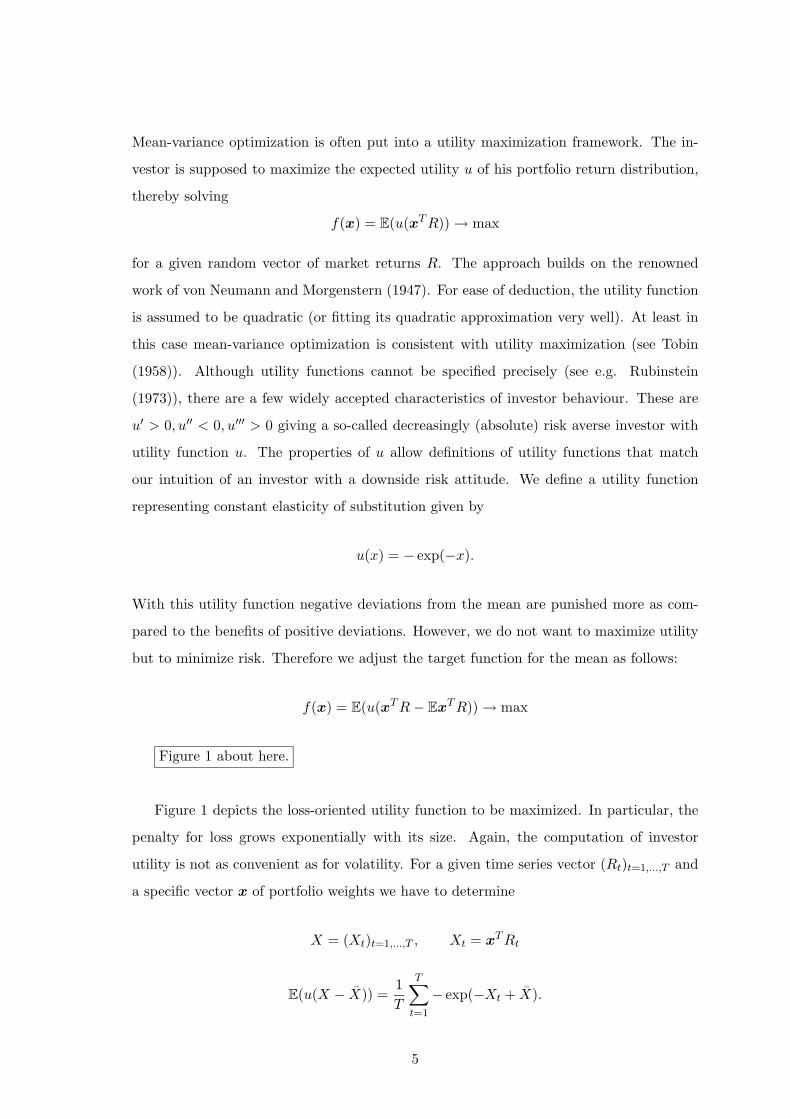
our intuition of an investor with a downside risk attitude. We define a utility function
representing constant elasticity of substitution given by
u(x) = − exp(−x).
With this utility function negative deviations from the mean are punished more as com-
pared to the benefits of positive deviations. However, we do not want to maximize utility
but to minimize risk. Therefore we adjust the target function for the mean as follows:
f(x) = E(u(xT R − ExT R)) → max
Figure 1 about here.
Figure 1 depicts the loss-oriented utility function to be maximized. In particular, the
penalty for loss grows exponentially with its size. Again, the computation of investor
utility is not as convenient as for volatility. For a given time series vector (Rt)t=1,...,T and
a specific vector x of portfolio weights we have to determine
X = (Xt)t=1,...,T , Xt = xT Rt
E(u(X − X)) =1
T
T∑
t=1
− exp(−Xt + X).
5
We emphasize that we do not claim to know the investor’s utility function. We rather
optimize a function having returns as arguments that fits our goal to mitigate downside
risks and can coincidentally be interpreted as one possible utility function.
Skewness
The skewness of a return distribution R is defined as
γ(R) =E
(
(R − ER)3)
σ(R)3/2.
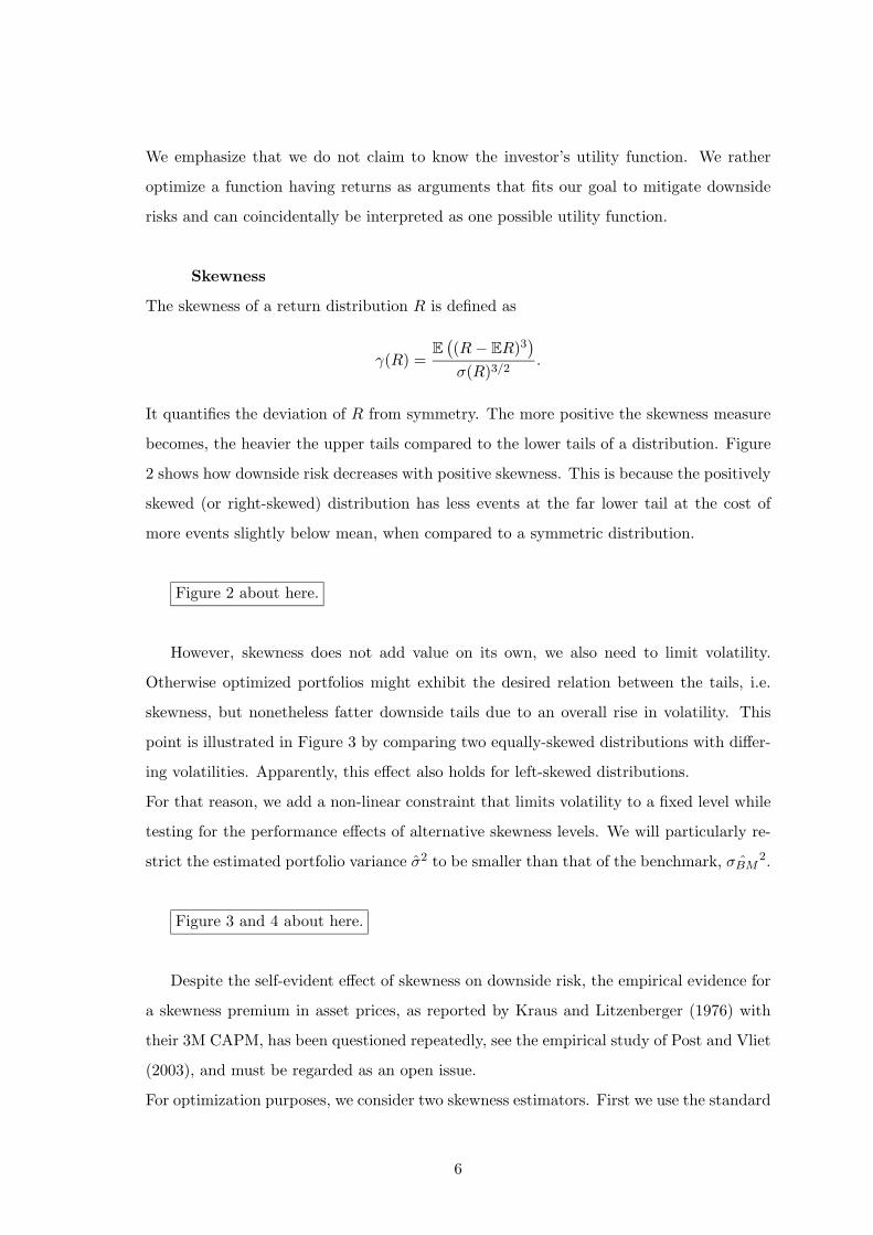
It quantifies the deviation of R from symmetry. The more positive the skewness measure
becomes, the heavier the upper tails compared to the lower tails of a distribution. Figure
2 shows how downside risk decreases with positive skewness. This is because the positively
skewed (or right-skewed) distribution has less events at the far lower tail at the cost of
more events slightly below mean, when compared to a symmetric distribution.
Figure 2 about here.
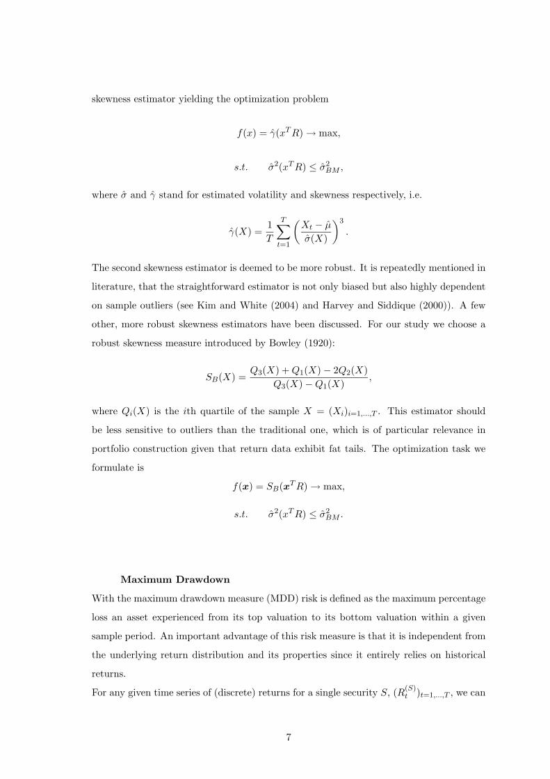
However, skewness does not add value on its own, we also need to limit volatility.
Otherwise optimized portfolios might exhibit the desired relation between the tails, i.e.
skewness, but nonetheless fatter downside tails due to an overall rise in volatility. This
point is illustrated in Figure 3 by comparing two equally-skewed distributions with differ-
ing volatilities. Apparently, this effect also holds for left-skewed distributions.
For that reason, we add a non-linear constraint that limits volatility to a fixed level while
testing for the performance effects of alternative skewness levels. We will particularly re-
strict the estimated portfolio variance σ2 to be smaller than that of the benchmark, ˆσBM2.
Figure 3 and 4 about here.
Despite the self-evident effect of skewness on downside risk, the empirical evidence for
a skewness premium in asset prices, as reported by Kraus and Litzenberger (1976) with
their 3M CAPM, has been questioned repeatedly, see the empirical study of Post and Vliet
(2003), and must be regarded as an open issue.
For optimization purposes, we consider two skewness estimators. First we use the standard
6
skewness estimator yielding the optimization problem
f(x) = γ(xT R) → max,
s.t. σ2(xT R) ≤ σ2BM ,
where σ and γ stand for estimated volatility and skewness respectively, i.e.
γ(X) =1
T
T∑
t=1
(
Xt − µ
σ(X)
)3
.
The second skewness estimator is deemed to be more robust. It is repeatedly mentioned in
literature, that the straightforward estimator is not only biased but also highly dependent
on sample outliers (see Kim and White (2004) and Harvey and Siddique (2000)). A few
other, more robust skewness estimators have been discussed. For our study we choose a
robust skewness measure introduced by Bowley (1920):
SB(X) =Q3(X) + Q1(X) − 2Q2(X)
Q3(X) − Q1(X),
where Qi(X) is the ith quartile of the sample X = (Xi)i=1,...,T . This estimator should
be less sensitive to outliers than the traditional one, which is of particular relevance in
portfolio construction given that return data exhibit fat tails. The optimization task we
formulate is
f(x) = SB(xT R) → max,
s.t. σ2(xT R) ≤ σ2BM .
Maximum Drawdown
With the maximum drawdown measure (MDD) risk is defined as the maximum percentage
loss an asset experienced from its top valuation to its bottom valuation within a given
sample period. An important advantage of this risk measure is that it is independent from
the underlying return distribution and its properties since it entirely relies on historical
returns.
For any given time series of (discrete) returns for a single security S, (R(S)t )t=1,...,T , we can
7
easily compute the corresponding time series of the portfolio value, if it solely consists of
security S. This value is given by
V(S)0 = 1, V
(S)t = V
(S)t−1(1 + R
(S)t /100), t = 1, . . . , T.3
In order to find out what was the worst period to be invested in S we calculate the MDD
for period [0, T ] recursively. Given the Maximum Drawdown for the period [0, T − 1],
MDD[0,T−1](S), we obtain
MDD[0,T ](S) = min
{
VT − Vt
Vt
, MDD[0,T−1](S)
}
, (2.1)
where Vt is the maximum value of the security held within [0, T − 1].
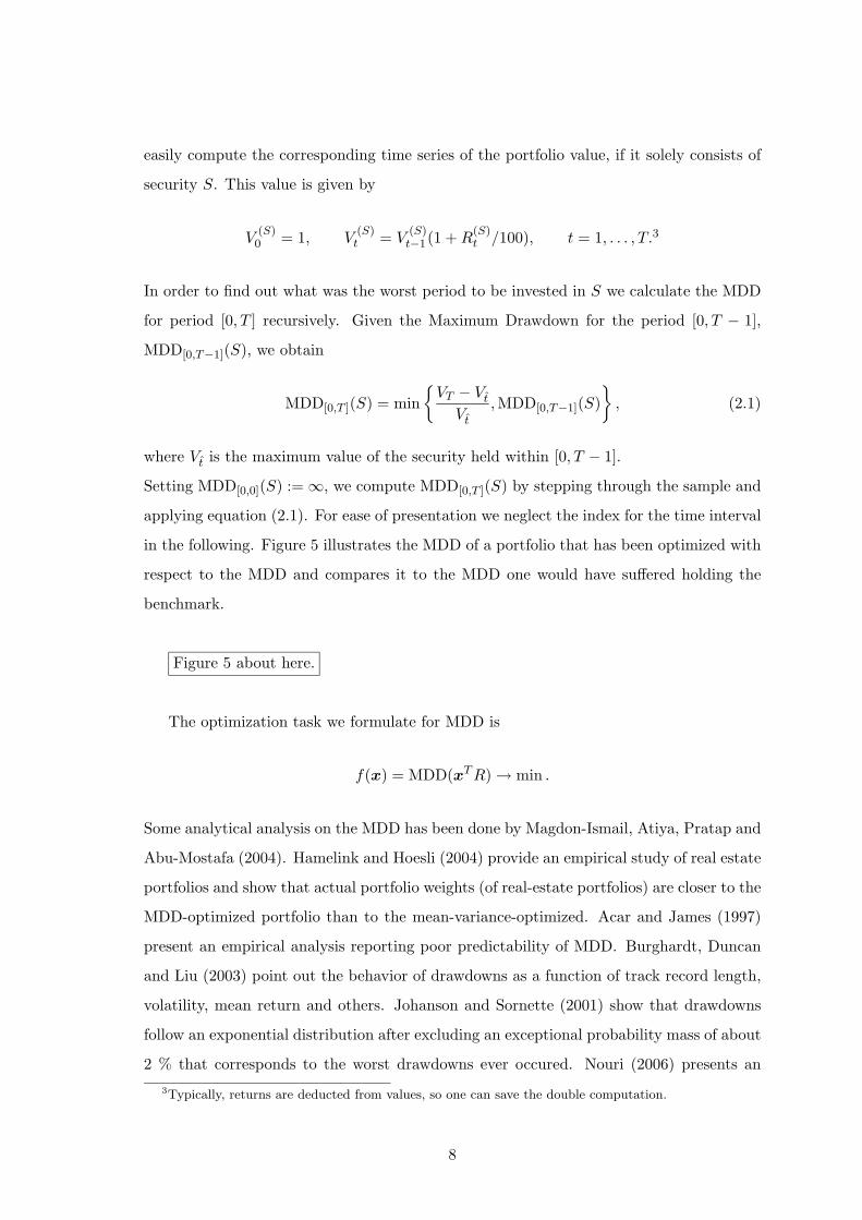
Setting MDD[0,0](S) := ∞, we compute MDD[0,T ](S) by stepping through the sample and
applying equation (2.1). For ease of presentation we neglect the index for the time interval
in the following. Figure 5 illustrates the MDD of a portfolio that has been optimized with
respect to the MDD and compares it to the MDD one would have suffered holding the
benchmark.
Figure 5 about here.
The optimization task we formulate for MDD is
f(x) = MDD(xT R) → min .
Some analytical analysis on the MDD has been done by Magdon-Ismail, Atiya, Pratap and
Abu-Mostafa (2004). Hamelink and Hoesli (2004) provide an empirical study of real estate
portfolios and show that actual portfolio weights (of real-estate portfolios) are closer to the
MDD-optimized portfolio than to the mean-variance-optimized. Acar and James (1997)
present an empirical analysis reporting poor predictability of MDD. Burghardt, Duncan
and Liu (2003) point out the behavior of drawdowns as a function of track record length,
volatility, mean return and others. Johanson and Sornette (2001) show that drawdowns
follow an exponential distribution after excluding an exceptional probability mass of about
2 % that corresponds to the worst drawdowns ever occured. Nouri (2006) presents an
3Typically, returns are deducted from values, so one can save the double computation.
8
analysis of expected drawdowns under constant and stochastic volatility.
3 Empirical Methodology
In our empirical study we investigate the characteristics of the portfolio construction ap-
proaches discussed above for a European equity portfolio to be managed against a bench-
mark.
We examine discrete weekly return data of the Dow Jones Euro Stoxx 50 universe from
January 1993 to April 2006 exclusive of ten names that have missing data for parts of the
period. For the remaining N = 40 stocks we adjust the index weights proportionally to
ensure that they sum up to 100 % and calculate adjusted benchmark returns accordingly.
For our empirical examination we adopt the following investment strategy. We optimize
portfolios under the risk measures defined above in a relative benchmark oriented setting
and require all optimization solutions to realize at least the benchmark return and to
satisfy a certain tracking error limit. The objective is to minimize risk according to the
respective risk definition.
We rely on an estimation period of two years (104 observations) to determine the risk
measures under investigation and reallocate the portfolio every three months (13 weeks).
We assume perfect foresight with respect to the return expectations but not with respect
to expected risk measures. Doing so we isolate the portfolio construction problem from the
return forecasting problem by assuming perfect return forecasts while the risk measures
under investigation are subject to empirical estimation based on past data.
To summarize, we examine six portfolio strategies based on the six objective functions
introduced in the last section, together with the traditional mean-variance approach using
volatility. Using X = xT R the optimization tasks are the following:
1. Volatility: f(x) = σ(X) = (xT Cx)1/2 → min,
2. Semivariance: f(x) = SV (X) = E(
(X − EX)2 | X < EX)
· P (X < EX) → min,
3. Semideviation: f(x) = SD(X) = E(X − EX | X < EX) · P (X < EX) → min,
4. Utility: f(x) = E(u(X − EX)) → max,
5. Standard skewness: f(x) = γ(X) = 1T
∑Tt=1
(
Xt − µσ(X)
)3→ min,
6. Robust skewness: f(x) = SB(X) =Q3 + Q1 − 2Q2
Q3 − Q1→ max,
7. Maximum Drawdown: f(x) = MDD(X) → min.
9
We include volatility in order to compare asymmetric risk measures also with Markowitz’
traditional measure. To complete the formulation of our optimization tasks we add the
following constraints:
First, we constrain the tracking error τ . For a given vector of benchmark portfolio weights
xBM and (optimized) weights x we restrict the tracking error by
τ(x) =√
(x − xBM )T C(x − xBM ) ≤ τmax.
The N × N−matrix C is the sample covariance matrix of the random vector of portfolio
returns.4 We set an annual tracking error limit of 5%.5 This leaves a fairly large discretion
to the optimizer to determine the weights and allows to obtain a quite clear picture about
the impact of the optimization process.
Second, we restrict the portfolio return to reach at least benchmark level, i.e.
µTx ≥ µ
TxBM .
Therefore the estimated mean return (and, in our case, under perfect foresight, a realized
return) of the optimized portfolio is greater or equal to the benchmark return. Note that
this constraint avoids optimization solutions to reduce risk at the cost of return. However,
it sets no incentive for the optimizer to go for higher returns on the other hand.
Third, when skewness is the objective we have already argued that volatility should be
limited as well. Thus, for optimization problems 5 and 6 we add the following constraint:
σ(x) =√
xT Cx ≤ σBM .
Beside these quadratic constraints we demand additional linear (in)equalities to be met.
These areN
∑
i=1
xi = 1 and xi ≥ 0 ∀i,
known as full investment and nonnegativity constraints. In summary, these assumptions
and restrictions imitate a portfolio manager who adjusts his portfolio every three months
for a certain risk objective and therefore considers data from a revolving two-year-period.
4We apply a straightforward estimator: σij = (T − 1)−1∑T
i=1(Ri − ERi)(Rj − ERj).
5We therefore appliy the rule for log-returns as a rule of thumb for discrete returns:τannual = τweekly ·
√
52. Since we optimize using weekly return and volatility data, the implementedtracking error limit is τmax = 5% ·
√
(52) = 0.69%.
10
Our methodology regarding the optimization process itself is rather pragmatic. We employ
Matlab’s flexible fmincon function for all alternatives except volatility for which we use
the quadprog function. fmincon offers a trust region method intended to tackle large scale
problems and a line search algorithm for medium scale tasks. After adjusting for the num-
ber of iterations and error tolerance, the medium scale method performed satisfactorily.
In other words, we do not spend much effort on streamlining the optimization itself but
focus on setting the objectives and interpreting the outcome.
4 Empirical Results
The results of the examined investment strategies are shown in Table 1 in a condensed form.
Table 1 about here.
The first three columns of Table 1 show the optimization impact on the average value
of the respective risk measures. They indicate that optimization decreases risk for most of
the considered objective functions. The average values of volatility, semideviation, semi-
variance, utility and Maximum Drawdown from optimized portfolios are far below the risk
levels of the benchmark. The fourth column of Table 1 shows, how much of the potential
percentage improvement in the risk measures under investigation is reached by the opti-
mization procedure. Scaling to percentages makes the rows comparable. Again, the five
examined risk measures show remarkable average improvement under optimization when
compared to simply buying and holding the benchmark.
However, for the two skewness related risk measures the average improvement is close to
zero and the deviation is in fact many times greater than the absolute value of improve-
ment (or impairment, if robust skewness is concerned). This indicates that skewness is
an unreliable property for the assets under scrutiny. Evidently, the sensitivity towards
sample outliers does not account for the lacking reliability of standard skewness. This can
be deducted from the paltry performance of the robust skewness measure on the other
hand. Robust skewness is the only measure that on average leads to a risk deterioration
of the optimized portfolio compared to the benchmark. Regarding loss-oriented utility, we
state a slightly worse performance compared to the remaining risk measures.
We do not want to go into more detail regarding the average improvement and deviation
11
figures. Since it is undue to compare percentage reductions in risk measures with different
growth characteristics. More precisely, loss-oriented utility grows exponentially, whereas
semivariance exhibits a quadratic increase, while semideviation grows linearly. Finally,
robust skewness is bounded by the interval [−1, 1].
Instead, we look at holding periods, where the objective function of the optimized port-
folio exhibits an improvement towards the benchmark. Note that the direction of change
does not say much about the accuracy of the predicted risk measures in absolute terms.
However, portfolio managers who compare their performance with benchmarks, are more
interested in benchmark-relative success anyway. These so called hit ratios are given in
the last column of Table 1.
For five out of seven investigated risk measures we find ratios far greater than 50%, in-
dicating a reduction of the respective risk measure in the vast majority of the cases. For
significance testing we assume that the number of intended objective changes is a realiza-
tion of a binomially distributed variable Y ∼ B(Z, p) with p = 0.5 and Z = 46, i.e. the
result of a random guess. To reject this hypothesis at the 5% (1%) level, Y needs to be
greater or equal to 29 (31). The improvement obtained from the examined optimization
procedures is significant for all risk measures under examination except for the skewness
related ones. Of the remaining measures, again only loss oriented utility performs little
worse than its competitors.
The results of Table 1 suggest that there is considerable persistence in the stock market
regarding various risk measures except for skewness-related ones.
To verify this hypothesis we examine the stability of the respective stock rankings, i.e. we
determine the ranking of the stock universe with respect to each risk measure and compare
the respective orders for all pairs of available consecutive years by means of Spearman’s
rank correlation coefficient. The results in Table 2 indicate that the risk measures showing
the highest correlation coefficient from period to period are volatility, semideviation and
semivariance, whereas skewness is not found to be persistent at all. These findings strongly
suggest that forecastability of employed risk measures is key for optimization procedures
to be practically applicable.
Table 2 about here.
If stock returns do not exhibit strong asymmetry or even come close to symmetry, it is
12

obvious that optimization with respect to portfolio semivariance is similar to optimization
with respect to variance. Moreover, the relationship between variance and semivariance
should be stronger in this case.
To examine the interdependence among examined risk measures in our sample, we estimate
linear regressions between
� semideviation versus volatility
� square root of semivariance versus volatility
� logarithm of expected (loss oriented) utility versus volatility
� maximum drawdown versus mean and volatility
and test these relationships in a cross-sectional regression at the single stock level. We use
four disjoint 3-year periods to estimate the respective historic risk measure values for each
of the 40 stocks included. We collect the regression results in Table 3.
Table 3 about here.
Table 3 reveals that semideviation can be virtually completely substituted by volatility
in the examined sample. Moreover, the more volatility-related risk measures in general
show higher reliability in the above tests. Semideviation and Semivariance perform ex-
cellently and show a tight relationship to volatility. Loss-oriented utility and maximum
drawdown exhibit significant reliability together with slight deficiencies. For these mea-
sures, only about two thirds of their deviation from the mean can be attributed to a linear
relationship with volatility.
5 Conclusion
Since investors are risk averse with respect to losses various asymmetric risk measures
focusing on downside risk have been proposed in the literature. In this paper we em-
pirically examined the characteristics of asymmetric risk measures such as semideviation,
semivariance, loss oriented utility, skewness measures as well as maximum drawdown in
an out-of-sample context. Our results indicate that portfolio optimization techniques may
successfully reduce asymmetric risk when compared to a strategy of buying and holding
a benchmark portfolio. This is in particular true for semideviation, semivariance, loss-
oriented utility as well as maximum drawdown while skewness risk is the hardest one to
13

control. Another important finding is that predictability of alternative risk measures is key
for their implementation in portfolio optimization processes. As we applied straightfor-
ward estimates derived from historic data for the investigated risk measures, in our case
predictability is synonymous with stability over time. Our empirical evidence suggests
that skewness measures are highly unstable over time. This observation even holds for a
more robust estimator of skewness with regard to outliers. As a consequence, we fail to
predict skewness risk properly and optimization fails to reduce skewness risk ex post.
Furthermore, given little asymmetry in equity returns the added value of alternative risk
measures compared to the traditional volatility measure might be limited. Note that if
asset returns are more or less symmetric we find alternative risk measures such as semi-
variance to be closely linked to the traditional volatility measure.
To summarize, alternative risk measures do a good job in portfolio optimization. In order
to improve their added value over traditional approaches future research should improve
the forecasting techniques for these measures on the one hand and should examine their
characteristics in the presence of asset returns facing strong asymmetry.
14
References
[1] Acar, E. and S. James (1997), Maximum Loss and Maximum Drawdown in Financial
Markets, Presented at the Forecasting Financial Markets Conference in London, May,
1997.
[2] Artzner, P., F. Delbaen, P. Embrechts and D. Heath (1999)Coherent Measures of Risk
Mathematical Finance, 9, 203-228.
[3] Bawa, V.S. and E.B. Lindenberg (1977), Capital Market Equilibrium in a Mean-Lower
Partial Moment Framework, Journal of Financial Economics, 5, 189-200.
[4] Bawa, V.S. (1978), Safety First, Stochastic Dominance and Optimal Portfolio Choice,
Journal of Financial and Quantitative Analysis, 13, 255-271.
[5] Bertsimas, D., G.J. Lauprete and A. Samarov (2004), Shortfall as a Risk Measure:
Properties, Optimization and Applications., Journal of Economic Dynamics & Control,
28, 1353-1381.
[6] Bos, T. and P. Newbold (1984), An Empirical Investigation of the Possibility of Sys-
tematic Stochastic Risk in the Market Model., Journal of Business, 57, 35-41.
[7] Bowley, A.L. (1920), Elements of Statistics, 4th ed., Charles Scribner’s sons, New York.
[8] Burghardt, B., R. Duncan and L. Liu, (2003), Deciphering Drawdowns, Risk Magazine,
September, 16-20.
[9] Ebner, M. and T. Neumann (2005), Time-Varying Betas of German Stock Returns,
Journal of Financial Markets and Portfolio Management, 19, 29-46.
[10] Fabozzi, F.J. and J.C. Francis (1978), Beta as a Random Coefficient, Journal of
Financial and Quantitative Analysis, 13, 101-115.
[11] Faff, R.W., Lee, J.H.H. and T.R.L. Fry (1992), Time Stationarity of Systematic Risk:
Some Australian Evidence, Journal of Business Finance and Accounting, 19, 253-270.
[12] Fama, E. (1965), The Behaviour of Stock Market Prices, Journal of Business, 38,
34-105.
[13] Fishburn, P. C. (1977), Mean-Risk Analysis with Risk Associated with Below-Target
Returns, American Economic Review, 67, 116-126.
15
[14] Guidolin, M. and A. Timmermann (2006), Term Structure of Risk under Alternative
Econometric Specifications, Journal of Econometrics, 131, 285-308.
[15] Hamelink, F. and M. Hoesli (2004), Maximum Drawdown and the Allocation to Real
Estate, Journal of Property Research, 21, 5-29.
[16] Harlow, W.V. and R.K.S. Rao (1989), Asset Pricing in a Generalized Mean-Lower
Partial Moment Framework: Theory and Evidence, Journal of Financial and Quanti-
tative Analysis, 24, 285-311.
[17] Harvey, C.R. and A. Siddique (2000), Conditional Skewness in Asset Pricing Tests,
Journal of Finance, 55, 1263-1295.
[18] Johansen, A. and D. Sornette (2001), Large Stock Market Price Drawdowns are Out-
liers, Journal of Risk, 4, 69-110.
[19] Kempf, A., Memmel, C. (2002), Schatzrisiken in der Portfoliotheorie in: Handbuch
Portfoliomanagement, Uhlenbruch.
[20] Kim, T.H. and H.White (2004), On More Robust Estimation of Skewness and Kurto-
sis, Finance Research Letters, 1, 56-70.
[21] Kraus, A. and R.H. Litzenberger (1976), Skewness Preference and the Valuation of
Risk Assets, Journal of Finance, 31, 1085-1100.
[22] Magdon-Ismail, M., A. Atiya, A. Pratap and Y. Abu-Mostafa (2004), On the Maxi-
mum Drawdown of a Brownian Motion., Journal of Applied Probability, 41, 147-161.
[23] Mandelbrot, B. (1963), The Variation of Certain Speculative Prices, Journal of Busi-
ness, 36, 394-419.
[24] Markowitz, H.M. (1952), Portfolio Selection, Journal of Finance, 7, 77-91.
[25] Markowitz, H.M. (1959), Portfolio Selection: Efficient Diversification of Investments,
New York: Wiley & Sons.
[26] Neumann, J. von, O. Morgenstern (1947), Theory of Games and Economic Behavior,
Princeton.
[27] Nouri, S. (2006), Expected Maximum Drawdowns under constant and stochastic
volatility, Thesis submitted in partial fulfillment of the requirements for the degree
16
of professional Masters degree in Financial Mathematics; Worchester Polytechnic In-
stitute, approved by Luis J. Roman.
[28] Ogryczak, W. and A. Ruszczynski (1998), On Stochastic Dominance and Mean-
Semideviation Models, Rutcor Research Report 7-98, February 1998.
[29] Post, T. and P. von Vliet (2003), Comment on Risk Aversion and Skewness Preference,
ERIM Report Series “‘Research in Management”’
[30] Rubinstein, M. (1973), A Comparative Statics Analysis of Risk Premiums., Journal
of Business, 46, 605-616.
[31] Schmidt von Rhein, A. (2002), Portfoliooptimierung mit der Ausfallvarianz, in: Hand-
buch Porfoliomanagement, Uhlenbruch.
[32] Schwert, G.W., and P.J. Seguin (1990), Heteroscedasticity in Stock Returns, Journal
of Finance, 45, 1129-1155.
[33] Tobin, J. (1958), Liquidity Preference as Behaviour Towards Risk, Review of Eco-
nomic Statistics, 25, 65–86.
[34] Wells, C. (1994), Variable Betas on the Stockholm Exchange 1971-1989, Applied Eco-
nomics, 4, 75-92.
17
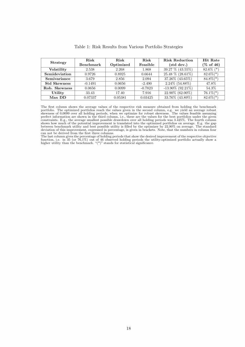
Table 1: Risk Results from Various Portfolio Strategies
StrategyRisk
BenchmarkRisk
OptimizedRisk
FeasibleRisk Reduction
(std dev.)Hit Rate(% of 46)
Volatility 2.538 2.268 1.868 39.27 % (43.55%) 82.6% (*)
Semideviation 0.9726 0.8925 0.6644 25.48 % (28.61%) 82.6%(*)
Semivariance 3.679 2.856 2.094 37.26% (43.65%) 84.8%(*)
Std Skewness -0.1491 0.0656 -2.490 2.24% (54.88%) 47.8%
Rob. Skewness 0.0656 0.0099 -0.7823 -13.90% (92.21%) 54.3%
Utility 33.43 17.40 7.916 22.90% (62.00%) 76.1%(*)
Max DD 0.07337 0.05381 0.03425 33.76% (43.89%) 82.6%(*)
The first column shows the average values of the respective risk measure obtained from holding the benchmarkportfolio. The optimized portfolios reach the values given in the second column, e.g. we yield an average robustskewness of 0,0099 over all holding periods, when we optimize for robust skewness. The values feasible assumingperfect information are shown in the third column, i.e., these are the values for the best portfolios under the givenconstraints. E.g., the average smallest possible drawdown over all holding periods was 3.425%. The fourth columnshows how much of the potential improvement is translated into the optimized portfolios on average. E.g. the gapbetween benchmark utility and best possible utility is filled by the optimizer by 22,90% on average. The standarddeviation of this improvement, expressed in percentage, is given in brackets. Note, that the numbers in column fourcan not be derived from the first three columns.The last column gives the percentage of holding periods that show the desired improvement of the respective objectivefunction, i.e. in 35 (or 76,1%) out of 46 observed holding periods the utility-optimized portfolio actually show ahigher utility than the benchmark. “(*)” stands for statistical significance.
18
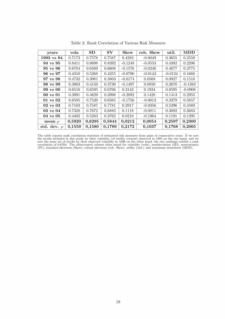
Table 2: Rank Correlation of Various Risk Measures
years vola SD SV Skew rob. Skew util. MDD
1993 vs 94 0.7173 0.7578 0.7587 0.4283 -0.0049 0.3655 0.2559
94 vs 95 0.8411 0.8698 0.8392 -0.1248 -0.0553 0.4392 0.2206
95 vs 96 0.6704 0.6569 0.6608 -0.1576 -0.0246 0.4677 0.3775
96 vs 97 0.4310 0.5268 0.4255 -0.0790 -0.0143 -0.0124 0.1668
97 vs 98 0.4732 0.3981 0.3803 -0.0174 0.0568 0.0927 0.1516
98 vs 99 0.3863 0.4150 0.3730 -0.1497 0.0850 0.2670 -0.1383
99 vs 00 0.6516 0.6595 0.6766 0.3143 0.1934 0.0595 -0.0908
00 vs 01 0.3991 0.4629 0.3998 -0.2092 0.1428 0.1413 0.2955
01 vs 02 0.6505 0.7520 0.6565 -0.1756 -0.0013 0.3379 0.5657
02 vs 03 0.7103 0.7587 0.7781 0.2917 -0.0356 0.5296 0.4569
03 vs 04 0.7328 0.7672 0.6882 0.1118 -0.0811 0.3092 0.3683
04 vs 05 0.4402 0.5283 0.3762 0.0218 -0.1964 0.1191 0.1295
mean ρ 0,5920 0,6295 0,5844 0,0212 0,0054 0,2597 0,2300
std. dev. ρ 0,1559 0,1580 0,1789 0,2172 0,1037 0,1768 0,2065
The table reports rank correlation statistics of estimated risk measures from pairs of consecutive years. If we sortthe stocks included in this study by their volatility (of weekly returns) observed in 1995 on the one hand, and wesort the same set of stocks by their observed volatility in 1996 on the other hand, the two rankings exhibit a rankcorrelation of 0.6704. The abbreviated column titles stand for volatility (vola), semideviation (SD), semivariance(SV), standard skewness (Skew), robust skewness (rob. Skew), utility (util.) and maximum drawdown (MDD).
19
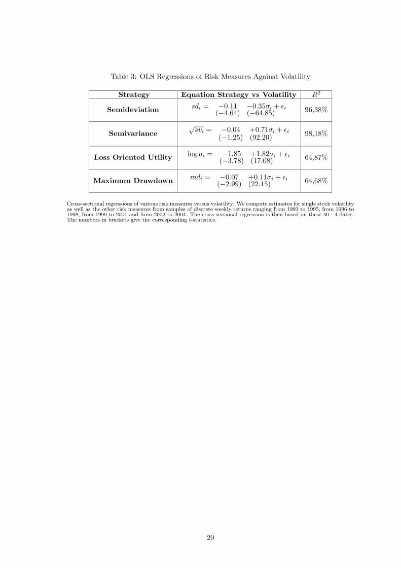
Table 3: OLS Regressions of Risk Measures Against Volatility
Strategy Equation Strategy vs Volatility R2
Semideviation sdi = −0.11 −0.35σi + εi(−4.64) (−64.85) 96,38%
Semivariance√
svi = −0.04 +0.71σi + εi
(−1.25) (92.20)98,18%
Loss Oriented Utilitylog ui = −1.85 +1.82σi + εi
(−3.78) (17.08) 64,87%
Maximum Drawdown mdi = −0.07 +0.11σi + εi(−2.99) (22.15) 64,68%
Cross-sectional regressions of various risk measures versus volatility. We compute estimates for single stock volatilityas well as the other risk measures from samples of discrete weekly returns ranging from 1993 to 1995, from 1996 to1998, from 1999 to 2001 and from 2002 to 2004. The cross-sectional regression is then based on these 40 · 4 dates.The numbers in brackets give the corresponding t-statistics.
20
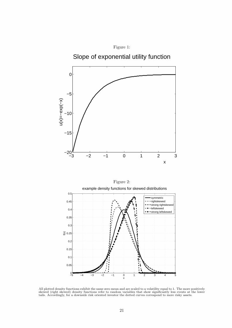
Figure 1:
−3 −2 −1 0 1 2 3−20
−15
−10
−5
0
x
u(x)
=−
exp(
−x)
Slope of exponential utility function
Figure 2:
−5 −4 −3 −2 −1 0 1 2 3 4 50
0.05
0.1
0.15
0.2
0.25
0.3
0.35
0.4
0.45
0.5
x
f(x)
example density functions for skewed distributions
symmetricrightskewedstrong rightskewedleftskewedstrong leftskewed
All plotted density functions exhibit the same zero mean and are scaled to a volatility equal to 1. The more positivelyskewed (right skewed) density functions refer to random variables that show significantly less events at the lowertails. Accordingly, for a downside risk oriented investor the dotted curves correspond to more risky assets.
21
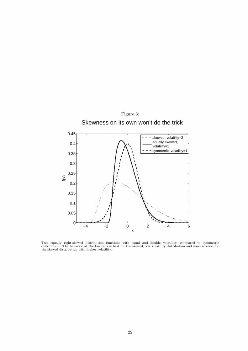
Figure 3:
−4 −2 0 2 4 60
0.05
0.1
0.15
0.2
0.25
0.3
0.35
0.4
0.45
Skewness on its own won’t do the trick
x
f(x)
skewed, volatility=2equally skewed,volatility=1symmetric, volatility=1
Two equally right-skewed distribution functions with equal and double volatility, compared to symmetricdistribution. The behavior at the low tails is best for the skewed, low volatility distribution and most adverse forthe skewed distribution with higher volatility.
22
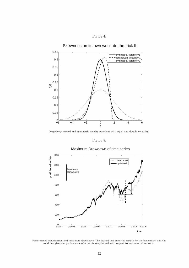
Figure 4:
−6 −4 −2 0 2 4 60
0.05
0.1
0.15
0.2
0.25
0.3
0.35
0.4
0.45
Skewness on its own won’t do the trick II
x
f(x)
symmetric, volatility=1leftskewed, volatility=1symmetric, volatility=2
Negatively skewed and symmetric density functions with equal and double volatility.
Figure 5:
1/1993 1/1995 1/1997 1/1999 1/2001 1/2003 1/2005 4/20060
200
400
600
800
1000
1200
1400
time
port
folio
val
ue (
%)
Maximum Drawdown of time series
benchmarkoptimized
MaximumDrawdown
Performance visualization and maximum drawdown: The dashed line gives the results for the benchmark and thesolid line gives the performance of a portfolio optimized with respect to maximum drawdown.
23