Portfolio choice under space-time monotoneperformance criteria�

M. Musielayand T. Zariphopoulouz

BNP Paribas, London and the University of Texas at Austin

November 15, 2008Previous title: Implied preferences and bespoke portfolios

Abstract

The class of time-decreasing forward performance processes is analyzedin a portfolio choice model of Ito-type asset dynamics. The associatedoptimal wealth and portfolio processes are explicitly constructed and theirprobabilistic properties discussed. These formulae are, in turn, used inanalyzing how the investor�s preferences can be calibrated to the market,given his desired investment targets.

1 Introduction

This paper is a contribution to portfolio management from the perspective ofinvestor preferences and, hence, in its spirit is related to the classical expectedutility maximization problem introduced by Merton ([8]). Therein, one �rstchooses an investment horizon and assigns a utility function at the end of itand, in turn, seeks an investment strategy which delivers the maximal expected(indirect) utility of terminal wealth. Recently, the authors proposed an alterna-tive approach to optimal portfolio choice which is based on the so-called forwardperformance criterion (see, among others, [10] and [9]). In this approach, theinvestor does not choose her risk preferences at a single point in time, as it isthe case in the Merton model, but has the �exibility to revise them dynamically.

�This work was presented at the 4th World Congress of BFS (2006) and at meetings andworkshops at, among others, U.C., Santa Barbara, U.M., College Park, Columbia University,MIT (2006), Oberwolfach, Stanford University, AMaMeF, QMF (2007) and Oberwolfach,University of Kostanz, RICAM (2008). The authors would like to thank the participantsfor fruitful suggestions and, especially, P. Carr and M. Yor. We, also, thank the researchassistants R. Popo¤ and T. Zhou for their comments.

yBNP Paribas, London; marek.musiela@bnpparibas.comzThe University of Texas at Austin; zariphop@math.utexas.edu. The second author ac-

knowledges partial support from the National Science Foundation (NSF grants: DMS-FRG-0456118 and DMS-RTG-0636586).

1

Herein, we focus on a speci�c case of a forward performance criterion, orig-inally introduced in [10] (see, also [12]). This criterion is a composition ofdeterministic and stochastic inputs. The deterministic input corresponds tothe investor�s preferences, or alternatively, to her tolerance towards risk. Itis investor speci�c, represented by a function, u (x; t) ; which is increasing andconcave in x; and decreasing in t: The stochastic input, however, is universalfor all investors and re�ects the objective statement about the market. It isrepresented by At =

R t0j�sj2 ds, t � 0; with �t being the Sharpe ratio of the

available for trading securities. The performance criterion is, then, given by theprocess Ut (x) = u (x;At) ; t � 0: Because of its form and the properties of theinvolved inputs, the performance process is monotone in wealth and time.Our contribution is threefold. Firstly, we provide a general characterization

of the di¤erential input function, u (x; t) : A space-time harmonic function playsa pivotal role in achieving this. This function is fully characterized by a positivemeasure which, in turn, becomes the underlying element in the speci�cation ofall quantities of interest. An important ingredient is the support of this measure,as it directly a¤ects the domain of the di¤erential input. We provide a detailedstudy of this interplay.The second contribution is the explicit construction of the optimal invest-

ment strategy and the associated optimal wealth. The speci�cation of theseprocesses is rather general as it does not rely on any Markovian assumptionson asset dynamics or on any speci�c structure of the investor�s input. To ourknowledge, this is one of the very rare cases in which such explicit formulae canbe derived in a model as general as the one considered herein.The third contribution is the initiation of a study on how we can learn

about the investor�s risk preferences from his investment goals. For example,the investor may want to specify the average level of wealth he could generate infuture times, in the particular market he chooses. This information is, then, usedto deduce his preferences which are consistent with this investment target. Suchinference problems are, in general, very hard to solve due to lacking closed formformulae, a di¢ culty that is surpassed herein due to the availability of explicitsolutions. It is important to notice that the assessment of market movementsis implicitly embedded in the investor�s desired investment goals. In manyaspects, this approach can be compared with the calibration of derivative pricingmodels. Indeed, therein, one also needs to make a statement about the marketunder the historical measure. Then, assuming no arbitrage, derivatives arevalued under the risk neutral measure, with the valuation requiring calibrationof the model to the observable market prices of the relevant assets. Thereis, however, an important di¤erence between the derivative pricing and theportfolio selection problem. In the latter, we cannot rely on the market to giveinformation about the investor�s individual preferences. However, we show howto acquire information about them by asking the investor to specify the desirableto her properties of the wealth process she wishes to generate.The criterion studied in this paper does not allow for arbitrary stochastic

evolution of preferences as the performance process is monotonically decreasingand, hence, its quadratic variation is equal to zero. To incorporate more �exibil-

2

ity, one needs to work with selection criteria in their full generality. Preliminaryresults in this direction can be found in [11].The paper is organized as follows. The model and the general portfolio

selection criteria are de�ned in the next section. In section 3, we present themonotone performance criterion and provide explicit solutions for the associatedoptimal wealth and portfolio processes. In section 4, we provide a detailedconstruction of the di¤erential input via the associated space-time harmonicfunction. In section 5, we analyze the case of deterministic market price ofrisk and discuss the distributional properties of the optimal wealth. We �nishwith discussing how the investor speci�c input can be inferred from targetedproperties of her future expected wealth.

2 The model and portfolio selection criteria

The market environment consists of one riskless and k risky securities. Theprices of risky securities are modelled as Ito processes. Namely, the price Si ofthe ith risky asset follows

dSit = Sit

0@�itdt+ dXj=1

�jit dWjt

1A ;with Si0 > 0 for i = 1; :::; k: The process Wt =

�W 1t ; :::;W

dt

�; t � 0; is a stan-

dard d�dimensional Brownian motion, de�ned on a �ltered probability space(;F ;P). The coe¢ cients �it and �it =

��1it ; :::; �

dit

�; i = 1; :::; k, t � 0; are

Ft�adapted processes with values in R and Rd, respectively. For brevity, wewrite �t to denote the volatility matrix, i.e., the d � k random matrix

��jit

�;

whose ith column represents the volatility �it of the ith risky asset. We may,

then, alternatively write the above equation as

dSit = Sit

��itdt+ �

it � dWt

�: (1)

The riskless asset, the savings account, has the price process B satisfying

dBt = rtBtdt;

with B0 = 1; and for a nonnegative, Ft�adapted interest rate process rt: Also,we denote by �t the k�dim vector with coordinates �it and by 1 the k�dimvector with every component equal to one. The processes, �t; �t and rt satisfythe appropriate integrability conditions.We assume that the volatility vectors are such that

�t � rt1 2 Lin��Tt�; (2)

where Lin��Tt�denotes the linear space generated by the columns of �Tt . This

implies that �Tt��Tt�+(�t � rt1) = �t � rt1 and, therefore, the vector

�t =��Tt�+(�t � rt1) (3)

3

is a solution to the equation �Tt x = �t � rt1: The matrix��Tt�+is the Moore-

Penrose pseudo-inverse1 of the matrix �Tt .Occasionally, we will be referring to �t as the market price of risk. It easily

follows that�t�

+t �t = �t (4)

and, hence, �t 2 Lin (�t). We assume throughout that the process �t is boundedby a deterministic constant c > 0; i.e., for all t � 0;

j�tj � c: (5)

Starting at t = 0 with an initial endowment x 2 R, the investor invests atany time t > 0 in the riskless and risky assets. The present value of the amountsinvested are denoted by �0t and �

it , i = 1; :::; k, respectively.

The present value of her investment is, then, given by X�t =

Pki=0 �

it; t > 0:

We will refer toX�t as the discounted wealth. The investment strategies will play

the role of control processes and are taken to satisfy the standard assumptionof being self-�nancing. Using (1) we, then, deduce that the discounted wealthsatis�es

dX�t =

kXi=1

�it�it � (�tdt+ dWt) = �t�t � (�tdt+ dWt) ; (6)

where the (column) vector, �t =��it; i = 1; :::; k

�: The set of admissible strate-

gies, A, is de�ned as

A =�� : self-�nancing with �t 2 Ft and E

�Z t

0

j�s�sj2 ds�<1; t > 0

�:

(7)The problem we propose to address is that of a choice of an investment

strategy from the set A. To this aim, we introduce below a process whichmeasures the performance of any admissible portfolio and gives us a selectioncriterion. Speci�cally, a strategy is deemed optimal if it generates a wealthprocess whose average performance is maintained over time. In other words,the average performance of this strategy at any future date, conditional ontoday�s information, preserves the performance of this strategy up until today.Any strategy that fails to maintain the average performance over time is, then,sub-optimal.

De�nition 1 An Ft�adapted process Ut (x) is a forward performance if fort � 0 and x 2 R:i) the mapping x! Ut (x) is strictly concave and increasing,ii) for each � 2 A; E (Ut (X�

t ))+<1; and

E (Us (X�s ) jFt ) � Ut (X�

t ) ; s � t; (8)

1See [13] and [7].

4

iii) there exists �� 2 A; for which

E�Us

�X��

s

�jFt�= Ut

�X��

t

�; s � t: (9)

We refer the reader to [10] for a detailed discussion on the new concept andits comparison to the classical value function (for the latter, see, among others,[8], [5] and [14]).

The de�nition of the forward performance process requires the integrabilityof (Ut (X�

t ))+: This allows us to de�ne the conditional expectations E (Us (X�

s ) jFt )for s � t and, in turn, obtain a more practical intuition for our criteria. Thisleads, however, to additional integrability assumptions which further constrainthe class of forward solutions the investor may employ. On the other hand,from the applications perspective, this may help in the calibration process ofthe investor�s initial risk preferences.Alternatively, and simpler from the mathematical view point, it would be

to replace conditions ii) and iii) above with corresponding local statements, asproposed next. To this end, we �rst relax the set of admissible strategies to

Al=�� : self-�nancing with �t 2 Ft and P

�Z t

0

j�s�sj2 ds <1�= 1; t > 0

�:

(10)

De�nition 2 An Ft�adapted process Ut (x) is a local forward performance iffor t � 0 and x 2 R:i) the mapping x! Ut (x) is strictly concave and increasing,ii) for each � 2 Al; the process Ut (X�

t ) is a local supermartingale, andiii) there exists �� 2 Al such that the process Ut

�X��

t

�is a local martingale.

Herein, we do not analyze the relaxed formulation of the problem but onlypresent an example of a local forward performance (see Example 12).Other modi�cations of the de�nition of the forward performance process are

possible, all based on the same principle, namely, to choose an investment strat-egy that keeps the expected investment performance constant across time. Forexample, one can relax or modify the assumption on monotonicity and (strict)concavity. This is desirable, in particular, for the development of time consis-tent behavioral portfolio selection models. A natural modi�cation would be toassume the existence of a reference point for the investor�s wealth that de�nesgains and losses (see, for example, [4]). The mapping x ! Ut (x) should be,then, concave for gains and convex for losses. The supermartingality conditionin the above de�nitions would have to be replaced by a statement about thesign of the drift in the semimartingale decomposition of Ut (X�

t ) : Speci�cally,the drift would be negative when the wealth is above the reference point andpositive when below. However, such modi�cations and extensions are beyondthe scope of this paper and are mentioned here only to expose the �exibility ofour de�nition.

5

We conclude mentioning that the classical Markowitz portfolio selectionproblem (see, among others [3] and [6]) could be also incorporated into ourframework. Indeed, one would need to choose the mean level of wealth and �ndthe portfolio that deviates from it the least, in the variance sense. Note thatnot all mean functions would be admissible, as it is already demonstrated inthis paper (however, with respect to criteria not covering the case of variance).The variance-based criteria deserve a separate treatment which will be carriedout in a future study.

3 Monotone performance processes and their op-timal wealth and portfolio processes

We focus on the class of time-decreasing performance processes introduced bythe authors in [10] (see, also [12] and [9]) and provide a full characterization ofthe associated optimal wealth and portfolio processes. As mentioned earlier, theperformance process, Ut (x) ; is constructed by compiling market related inputwith a deterministic function of space and time, namely, for t � 0;

Ut (x) = u (x;At) ;

where u (x; t) is increasing and strictly concave in x; and satis�es

ut =1

2

u2xuxx

; (11)

with At as in (13) below.The main contribution of this section is the explicit construction of the

optimal wealth and portfolio processes, denoted respectively by X�t and �

�t ;

t � 0: We establish that, in analogy to the forward performance process, theseprocesses are, also, given as a compilation of market input and deterministicfunctions of space and time. Namely, we show that

X�t = h

�h(�1) (x; 0) +At +Mt; At

�and ��t = hx

�h(�1) (X�

t ; At) ; At

��+t �t;

where h (x; t) is strictly increasing in x and solves the (backward) heat equation

ht +1

2hxx = 0; (12)

for (x; t) 2 R� [0;+1) : The function h(�1) stands for the spatial inverse of h:The market input processes At and Mt; t � 0; are de�ned as

At =

Z t

0

j�sj2 ds and Mt =

Z t

0

�s � dWs; (13)

with �t as in (3).

6

The above formulae demonstrate that all quantities of interest can be fullyspeci�ed as long as the market price of risk is chosen and the functions u and hare known. A considerable part of this paper is, thus, dedicated to the study ofthese functions and, especially, their representation and connection with eachother.For the reader�s convenience, we choose to present these results separately,

in the next section. Speci�cally, it is shown therein (see Propositions 9, 13, 14and 18) that there exists a one-to-one correspondence (modulo normalizationconstants) between increasing and strictly concave solutions to (11) with strictlyincreasing solutions to (12). It is, also, shown that the latter can be representedin terms of the bilateral Laplace transform of a positive �nite Borel measure,denoted by �. This measure then emerges as the de�ning element in the entireanalysis of the problem at hand. Its presence originates from the classical resultsof Widder (see Chapter XIV in [17]) on the construction of positive solutions tothe heat equation (12). In the investment model we consider, the solution h of(12) represents the optimal wealth which, however, might take arbitrary values.As a result, a more detailed study is required depending on the range of h.We proceed with the main theorem in which we provide the optimal wealth,

the associated optimal investment strategy and the space-time monotone for-ward performance process. We state the result without making speci�c referenceto the range of h, as well as the domain and range of u; as the di¤erent casesare analyzed in detail later. We, also, do not make any reference to the regular-ity of these functions since the required smoothness follows trivially from theirrepresentation.We stress, however, that we introduce the integrability condition (14). This

condition is stronger than the one needed for the representations of h (cf. (26)),and in turn of u; but su¢ cient in order to guarantee the admissibility of thecandidate optimal policy (16). It may be relaxed if, for example, one chooses towork instead with local forward performance processes, introduced in De�nition2. For additional comments on condition (14) see the discussion after Example12.

Theorem 3 i) Let h be a strictly increasing solution to (12), for (x; t) 2R� [0;+1) ; and assume that the associated measure � satis�esZ

Reyx+

12y

2t� (dy) <1: (14)

Let also At and Mt; t � 0; be as in (13) and de�ne the processes X�t and �

�t by

X�t = h

�h(�1) (x; 0) +At +Mt; At

�(15)

and��t = hx

�h(�1) (X�

t ; At) ; At

��+t �t; (16)

t � 0; x 2 R with h as above and h(�1) standing for its spatial inverse. Then,

7

the portfolio ��t is admissible and generates X�t ; i.e.,

X�t = x+

Z t

0

�s��s � (�sds+ dWs) : (17)

ii) Let u be the associated with h increasing and strictly concave solution to(11). Then, the process u (X�

t ; At) ; t � 0; satis�es

du (X�t ; At) = ux (X

�t ; At)�t�

�t � dWt; (18)

with X�t and �

�t as in (15) and (16).

iii) Let Ut (x), t � 0; x 2 R be given by

Ut (x) = u (x;At) : (19)

Then, Ut (x) is a forward performance process and the processes X�t and �

�t are

optimal.

Proof. We provide the proof only when h is of in�nite range since the cases ofsemi-in�nite range can be worked out by analogous arguments.As it was mentioned earlier, the representation of h is established in the next

section. When h is of in�nite range, it is given in Proposition 7, (cf. (30)),rewritten below for convenience, namely,

h (x; t) =

ZR

eyx�12y

2t � 1y

� (dy) ;

for (x; t) 2 R� [0;+1) (for simplicity we take C = 0 in (30)):For x 2 R, At and Mt as in (13), we, then, de�ne the process

Nt = h(�1) (x; 0) +At +Mt;

where h(�1) is the spatial inverse of h: Applying Ito�s formula to X�t ; given in

(15), and using (12) yields

dX�t = hx (Nt; At) dNt: (20)

On the other hand, (15) and (16) imply

��t = hx (Nt; At)�+t �t;

t � 0; and (17) follows from the above and (4).To establish that ��t 2 A; it su¢ ces to show that the integrability condition

in (7) is satis�ed. Using that

hx (x; t) =

ZReyx�

12y

2t� (dy)

(cf. (34)) and (15) we have�hx

�h(�1) (X�

t ; At) ; At

��28

=

ZR

ZRe(y1+y2)(h

(�1)(x;0)+At+Mt)� 12 (y

21+y

22)At� (dy1) � (dy2) :

From (4), Fubini�s theorem and (13), we deduce

E

�Z t

0

j�s��sj2ds

�= E

�Z t

0

���hx �h(�1) (X�s ; As) ; As

��s�

+s �s

���2 ds�

= E

�Z t

0

�hx

�h(�1) (X�

s ; As) ; As

��2dAs

�=

ZR

ZRE

�Z t

0

e(y1+y2)(h(�1)(x;0)+As+Ms)� 1

2 (y21+y

22)AsdAs

�� (dy1) � (dy2)

=

ZR

ZRE

Z At

0

e(y1+y2)(h(�1)(x;0)+s+�s)� 1

2 (y21+y

22)sds

!� (dy1) � (dy2) ;

where �t =MA(�1)t

and A(�1)t stands for the inverse of At; t � 0: Using that �t;t � 0; is a Brownian motion on (; fFtg ;P) and (5), we obtain

E

�Z t

0

j�s��sj2ds

�

�ZR

ZRE

Z c2t

0

e(y1+y2)(h(�1)(x;0)+s+�s)� 1

2 (y21+y

22)sds

!� (dy1) � (dy2)

=

Z c2t

0

ZR

ZRe(y1+y2)(h

(�1)(x;0)+s)+y1y2s� (dy1) � (dy2) ds

�Z c2t

0

�ZRey(h

(�1)(x;0)+s)+ 12y

2s� (dy)

�2ds;

and using (14) we conclude.ii) The facts that u satis�es (11) and has the claimed monotonicity and

strict concavity properties are established separately, in Proposition 9, where adetailed construction of this function is presented.To show (18), we apply Ito�s formula to u (X�

t ; At) ; t � 0: To this end, using(20) yields

du (X�t ; At) = ux (X

�t ; At) dX

�t + ut (X

�t ; At) dAt +

1

2uxx (X

�t ; At) d hX�it

= ux (X�t ; At)hx

�h(�1) (X�

t ; At) ; At

��t � dWt

+ux (X�t ; At)hx

�h(�1) (X�

t ; At) ; At

�dAt

+ut (X�t ; At) dAt +

1

2uxx (X

�t ; At) d hX�it :

9

From (48) in the proof of Proposition 9, we deduce that

� ux (X�t ; At)

uxx (X�t ; At)

= hx

�h(�1) (X�

t ; At) ; At

�; (21)

which combined with the above yields

du (X�t ; At) = ux (X

�t ; At)hx

�h(�1) (X�

t ; At) ; At

��t � dWt

� (ux (X�t ; At))

2

uxx (X�t ; At)

dAt + ut (X�t ; At) dAt +

1

2uxx (X

�t ; At) d hX�it :

On the other hand, (20) gives

uxx (X�t ; At) d hX�it = uxx (X

�t ; At)

�hx

�h(�1) (X�

t ; At) ; At

��2dAt

=(ux (X

�t ; At))

2

uxx (X�t ; At)

dAt:

Therefore,

du (X�t ; At) = ux (X

�t ; At)hx

�h(�1) (X�

t ; At) ; At

��t � dWt

+

ut (X

�t ; At)�

1

2

(ux (X�t ; At))

2

uxx (X�t ; At)

!dAt;

and (18) follows since u satis�es (11).iii) We need to establish that Ut (x) satis�es all conditions in De�nition 1.

The facts that u (x;At) is Ft�adapted and that the mapping x ! u (x;At) isincreasing and strictly concave follow trivially from the properties of u and At.To establish the integrability condition E (Ut (X�

t ))+< 1; we work as fol-

lows. We �rst observe that the strict concavity of u together with (11) yieldsut < 0 and, hence, u (x; t) � u (x; 0) � ax+ + b; for some positive constants aand b: Also, (6) implies

(X�t )+ � x+ + 1

2

Z t

0

j�s�sj2 ds+1

2

Z t

0

j�sj2 ds+����Z t

0

�s�s � dWs

���� :The integrability of E (Ut (X�

t ))+ then follows using (5) and that �t 2 A:

To show (8), we observe that for �t 2 A and X�t as in (6), Ito�s formula

yields

du (X�t ; At) =

�ux (X

�t ; At)�t�t � �t + ut (X�

t ; At) j�tj2+1

2uxx (X

�t ; At) j�t�tj

2

�dt

+ux (X�t ; At)�t�t � dWt

10

=

ux (X

�t ; At)�t�t � �t +

1

2

(ux (X�t ; At))

2

uxx (X�t ; At)

j�tj2 +1

2uxx (X

�t ; At) j�t�tj

2

!dt

+ux (X�t ; At)�t�t � dWt

=1

2uxx (X

�t ; At)

�����t�t + ux (X�t ; At)

uxx (X�t ; At)

�t

����2 dt+ ux (X�t ; At)�t�t � dWt;

where we used that u solves (11). Using the concavity of u we conclude.To show (9) we use the form of the above drift, (21) and (16).Remark: We remind the reader that the forward performance process in [10]

is more general than the above, namely, it is given by

Ut (x) = u

�x

Yt; ~At

�Zt;

where the processes (Yt; Zt) are arbitrary and represent, respectively, a bench-mark (or numeraire) and alternative market views. They solve

dYt = Yt�t � (�tdt+ dWt) and dZt = Zt�t � dWt;

with Y0 = Z0 = 1 and �t; �t being Ft�adapted processes, satisfying �t�+t �t = �tand �t�

+t �t = �t; t � 0: The process ~At has a similar form to (13),

~At =

Z t

0

j�s + �s � �sj2ds:

Herein, we assume, throughout, �t = �t = 0; t � 0; as we focus on monotone intime forward performance processes.

The explicit formulae (15) and (16) enable us to analyze the mappings x!X�t (!) and x ! ��t (!) ; for �xed t and !: We study this dependence next.

To ease the presentation, we only discuss the case Range (h) = (�1;+1) :We also use the notation X�;x

t (!) and ��;xt ; and introduce the function, r :R� [0;+1)! (0;+1) ; de�ned as

r (x; t) = hx

�h(�1) (x; t) ; t

�: (22)

A detailed discussion on its role, representation and di¤erential propertiesis provided in section 4.5. Using (22), the optimal portfolio (cf. (16)) can be,then, written, for t � 0; as

��;xt = r�X�;xt ; At

��+t �t: (23)

Proposition 4 Let X�;xt be given in (15), t � 0; and r as in (22). Then,

@

@xX�;xt =

r�X�;xt ; At

�r (x; 0)

(24)

and@

@x��;xt = rx

�X�;xt ; At

� r �X�;xt ; At

�r (x; 0)

�+t �t: (25)

11

Proof. Di¤erentiating (15) with respect to x yields

@

@xX�;xt = hx

�h(�1) (x; 0) +At +Mt; At

� @

@xh(�1) (x; 0) ;

and (24) follows from (22). To establish (25) we di¤erentiate (23) and use (24).

The above result implies that the mapping x ! X�;xt is increasing. This is

to be expected because the larger the initial endowment the larger the futurewealth should be. It, also, shows that the mapping x ! ��;xt is increasing (ordecreasing) depending on the monotonicity of the function r: In general, thelatter is not monotone and, therefore, nothing speci�c can be said about thedependence of the optimal allocation in terms of the initial endowment2 . Themonotonicity holds, however, in a special but frequently considered case, namely,when there is no bankruptcy, or more generally when the wealth stays alwaysabove a certain threshold. This case is considered in Proposition 22 herein whereit is shown that rx � 0 (see (75)). As a result, the mapping x! ��;xt is alwaysincreasing. Respectively, the other results in the same proposition show that themapping x! ��;xt is always decreasing if the wealth stays below a threshold.The optimal wealth formula (15) enables us to calculate higher order deriv-

atives. For example, the second order derivative is given below.

Proposition 5 Let X�;xt ; t � 0; be given in (15) and r as in (22). Then,

@2

@x2X�;xt =

�rx�X�;xt ; At

�� rx (x; 0)

�r (x; 0)

@

@xX�;xt :

Proof. Di¤erentiating (24) yields

@2

@x2X�;xt =

rx�X�;xt ; At

�r (x; 0)

@

@xX�;xt � rx (x; 0)

r (x; 0)

r�X�;xt ; At

�r (x; 0)

;

and we easily conclude using (24) once more.

Representation (15) reveals how the market input processes, At and Mt;t � 0; interact with the deterministic input, h; to generate the optimal wealthprocess. The function h is, on the other hand, fully speci�ed by the measure�. It is, then, natural to ask how the function h and, in turn, the process X�

t ;t � 0; depend on the total mass � (R) :The result below shows an interesting scaling property which allows us to

normalize the function h and assume that � is a probability measure. Forsimplicity, we only discuss the case Range(h) = (�1;+1) :Let h0 = � (R) and denote, with a slight abuse of notation, the associated

wealth process by X�t (x;h0) ; t � 0:

2See, for example, the case r (x; t) =pax2 + be�at analyzed in [18].

12

Proposition 6 For h0 = � (R) ; the optimal wealth process (cf. (15)) satis�es,for t � 0;

1

h0X�t (x;h0) = X

�t

�x

h0; 1

�:

Proof. Let h (x; t) = h(x;t)h0

. Then,

X�t (x;h0) = h0h

�h(�1) (x; 0) +At +Mt; At

�:

On the other hand, h(�1) (x; 0) = h(�1) � x

h0; 0�and, hence,

X�t (x;h0) = h0h

�h(�1)

�x

h0; 0

�+At +Mt; At

�= h0X

�t

�x

h0; 1

�:

4 Representation of the functions u and h

The functions u and h (see Theorem 3) were instrumental in the constructionof the forward performance, and the associated optimal wealth and portfolioprocesses. In this section, we focus on the representation of these functionsand connection with each other. We recall that they satisfy (11) and (12),respectively, and that we are interested in solutions of (11) that are increasingand strictly concave in their spatial argument. We will show that there is a one-to-one correspondence (modulo normalization constants) between this class andstrictly increasing solutions to the (backward) heat equation (12).As it was mentioned in the previous section, the key idea is to represent h

in terms of a �nite positive Borel measure � and, in turn, construct u from h(see, for example, (30) and (43), respectively). This measure, then, emerges asthe de�ning element in the construction of any object of interest. The mainassumption about it is that its bilateral Laplace transform exists3 . Namely, wewill be working throughout this section with measures belonging to B+ (R) ;de�ned as

B+ (R)=�� 2 B (R) : 8B 2 B; � (B) � 0 and

ZReyx� (dy) <1; x 2 R

�:

(26)

The connection between � and h was established by Widder (see, for ex-ample, [17]) for nonnegative solutions of (12). However, these results cannotbe applied directly herein since, for the investment applications we consider,the wealth may not be assumed to remain always positive or, more generally,

3We remind the reader that this condition is su¢ cient for the �niteness of h and u but doesnot, in general, guarantee admissibility of the associated policies. For the latter, condition(14) is used.

13

stay above (or below) a given threshold. As a consequence, di¤erent choices forthe range of h; which represents the optimal wealth (cf. (15)), require di¤erentanalysis and are, therefore, examined separately below.We start with the general theorem which gives us the representation of

strictly increasing solutions to the heat equation (12). We introduce the fol-lowing sets,

B+0 (R) =�� 2 B+ (R) and � (f0g) = 0

; (27)

B++ (R) =�� 2 B+0 (R) : � ((�1; 0)) = 0

(28)

andB+� (R) =

�� 2 B+0 (R) : � ((0;+1)) = 0

: (29)

In what follows C represents a generic constant. Special choices for it are dis-cussed later on.

Proposition 7 i) Let � 2 B+ (R). Then, the function h de�ned, for (x; t) 2R� [0;+1) ; by

h (x; t) =

ZR

eyx�12y

2t � 1y

� (dy) + C; (30)

is a strictly increasing solution to (12).Moreover, if � (f0g) > 0; or � 2 B++ (R) and

R +10+

�(dy)y = +1; or � 2

B+� (R) andR 0��1

�(dy)y = �1; then Range (h) = (�1;+1) ; for t � 0:

On the other hand, if � 2 B++ (R) withR +10+

�(dy)y < +1 (resp. � 2

B+� (R) withR 0��1

�(dy)y > �1)); then Range (h) =

�C �

R +10+

�(dy)y ;+1

�(resp.

Range (h) =��1; C �

R 0��1

�(dy)y

�); for t � 0:

ii) Conversely, let h : R � [0;+1) ! R be a strictly increasing solution to(12). Then, there exists � 2 B+ (R) such that h is given by (30).Moreover, if Range (h) = (�1;+1) ; t � 0; then it must be either that

� (f0g) > 0, or � 2 B++ (R) andR +10+

�(dy)y = +1; or � 2 B+� (R) and

R 0��1

�(dy)y =

�1:On the other hand, if Range (h) = (x0;+1) (resp. Range (h) = (�1; x0)),

t � 0 and x0 2 R; then it must be that � 2 B++ (R) withR +10+

�(dy)y < +1 (resp.

� 2 B+� (R) withR 0��1

�(dy)y > �1).

Proof. i) Without loss of generality, we take C = 0: We �rst establish thath (x; t) is well de�ned: Indeed, for (x; t) 2 R� [0;+1) ; we haveZ

R

�����eyx�12y

2t � 1y

����� � (dy) =Zjyj>1

�����eyx�12y

2t � 1y

����� � (dy) (31)

14

+

Zjyj�1

�����eyx�12y

2t � 1y

����� � (dy) :On the other hand, one can show that, for �xed (x; t) and jyj � 1; the inequality�����eyx�

12y

2t � 1y

����� � ejxj+ t2 � 1 (32)

holds4 . Combining the above, we deduceZR

�����eyx�12y

2t � 1y

����� � (dy) �Zjyj>1

eyx� (dy) + � (R) ejxj+t2 < +1: (33)

Di¤erentiating under the integral yields

hx (x; t) =

ZReyx�

12y

2t� (dy) (34)

and the claimed monotonicity of h follows. Note that hx (x; t) is well de�nedbecause 0 � hx (x; t) < hx (x; 0) < +1, as � 2 B+ (R) : Further di¤erentiationyields

hxx (x; t) =

ZRyeyx�

12y

2t� (dy) and ht (x; t) = �1

2

ZRyeyx�

12y

2t� (dy) :

The fact that h solves (12) would follow provided the above integrals are wellde�ned. For x 6= 0; we have����Z

Ryeyx�

12y

2t� (dy)

���� � 1

jxj

ZRjyxj eyx� 1

2y2t� (dy)

� 1

jxj

ZR

�ejyxj � 1

�eyx�

12y

2t� (dy)

� 1

jxj

�Zyx�0

�ejyxj � 1

�eyx�

12y

2t� (dy) +

Zyx>0

�ejyxj � 1

�eyx�

12y

2t� (dy)

�� 1

jxj

�Zyx�0

(1� eyx) e� 12y

2t� (dy) +

Zyx>0

e2yx�12y

2t� (dy)

�� 1

jxj

Zyx�0

� (dy) +1

jxj

Zyx>0

e2yx� (dy) ;

and the assertion follows using that � 2 B+ (R). The case x = 0 follows trivially.

4 Indeed, we have eyx� 1

2y2t�1y

=P1n=1

yn�1(x� 12yt)n

n!and, therefore,

���� eyx� 12y2t�1y

���� �P1n=1

jyjn�1jx� 12ytjn

n!�P1n=1

(jxj+ 12jyjt)n

n!� ejxj+

t2 � 1:

15

Next, we establish that if � has the aforestated properties then, for eacht � 0; h is of full range. Given that h is continuous, we need to show that, fort � 0;

limx!�1

h (x; t) = �1 and limx!+1

h (x; t) = +1: (35)

From (30) we have

h (x; t) =

Z 0�

�1

eyx�12y

2t � 1y

� (dy)+x� (f0g)+Z +1

0+

eyx�12y

2t � 1y

� (dy) : (36)

We �rst look at the case � (f0g) > 0: If both � ((�1; 0)) = 0 and � ((0;+1)) =0; (35) follows directly. If � ((�1; 0)) = 0 and � ((0;+1)) > 0; the monotoneconvergence theorem gives

limx!�1

x� (f0g) +

Z +1

0+

eyx�12y

2t � 1y

� (dy)

!= �1:

The case � ((�1; 0)) > 0 and � ((0;+1)) = 0 follows similarly.Next, we assume � 2 B+0 (R) : Then, (36) yields

h (x; t) =

Z 0�

�1

eyx�12y

2t � 1y

� (dy) +

Z +1

0+

eyx�12y

2t � 1y

� (dy) ;

and we easily deduce (35) if � ((�1; 0))� � ((0;+1)) > 0:If � 2 B+0 (R) and it, also, satis�es � ((�1; 0)) = 0 and

R +10+

1y� (dy) = +1;

then the monotone convergence theorem yields

limx!+1

h (x; t) = limx!+1

Z +1

0+

eyx�12y

2t � 1y

� (dy) = +1

and

limx!�1

h (x; t) = �Z +1

0+

1

y� (dy) = �1:

The case � 2 B+� (R) withR 0��1

1y� (dy) = �1 follows similarly as well as the

cases � 2 B++ (R) withR +10+

1y� (dy) < +1; and � 2 B

+� (R) with

R 0��1

1y� (dy) >

�1:ii) Let h be a strictly increasing solution to (12). Then, its spatial derivative

satis�es hx (x; t) � 0 and solves (12). Thus, Widder�s theorem implies theexistence of � 2 B+ (R) such that the representation

hx (x; t) =

ZReyx�

12y

2t� (dy) (37)

holds. We, then, have hxx (x; t) =RR ye

yx� 12y

2t� (dy) (its �niteness followseasily) which combined with (12) yields

ht (x; t) = �1

2

ZRyeyx�

12y

2t� (dy) :

16

If Range (h) = (�1;+1) ; t � 0; integrating yields

h (x; t) =

Z t

0

ht (x; s) ds+

Z x

x0

hx (z; 0) dz + h (x0;0) ; (38)

for any x0 2 R: Combining the above we obtain

h (x; t) = �12

Z t

0

ZRyeyx�

12y

2s� (dy) ds+

Z x

x0

ZReyz (dy) dz + h (x0; 0) : (39)

Note that for � 2 B+ (R) ;Z t

0

ZR

���yeyx� 12y

2s��� � (dy) ds � tZ

Rjyj eyx� (dy) <1;

and, thus, Fubini�s theorem yields

�12

Z t

0

ZRyeyx�

12y

2s� (dy) ds = �12

ZR

Z t

0

yeyx�12y

2sds� (dy)

=

ZR

eyx�12y

2t � eyxy

� (dy) :

Moreover, Tonelli�s theorem yieldsZ x

x0

ZReyz� (dy) dz =

ZR

Z x

x0

eyzdz� (dy) =

ZR

eyx � eyx0y

� (dy) :

Observe that both integrals above are well de�ned as it was shown in the proofof part i). Using (39) gives

h (x; t) =

ZR

eyx�12y

2t � eyx0y

� (dy) + h (x0; 0) :

Without loss of generality we choose x0 = 0 and we easily conclude.Next, we establish that if h is of full range, for each t � 0; it must be that

� (f0g) > 0, or, otherwise, either � 2 B++ (R) withR +10+

1y� (dy) = +1; or

� 2 B+� (R) withR 0��1

1y� (dy) = �1: Note that (35) must hold, for each t � 0;

as h is continuous.Let us assume that � 2 B++ (R) and

R +10+

1y� (dy) < +1: Then, (36) would

give

limx!�1

h (x; t) = limx!�1

Z +1

0+

eyx�12y

2t � 1y

� (dy) = �Z +1

0+

1

y� (dy) > �1;

contradicting (35). All other cases follow along similar arguments and theirproof is, thus, omitted.

The following auxiliary result will be used in the sequel. Because we willexamine the various cases of the range of h separately, we state the resultwithout making speci�c reference to the domain of the spatial inverse, h(�1):

17

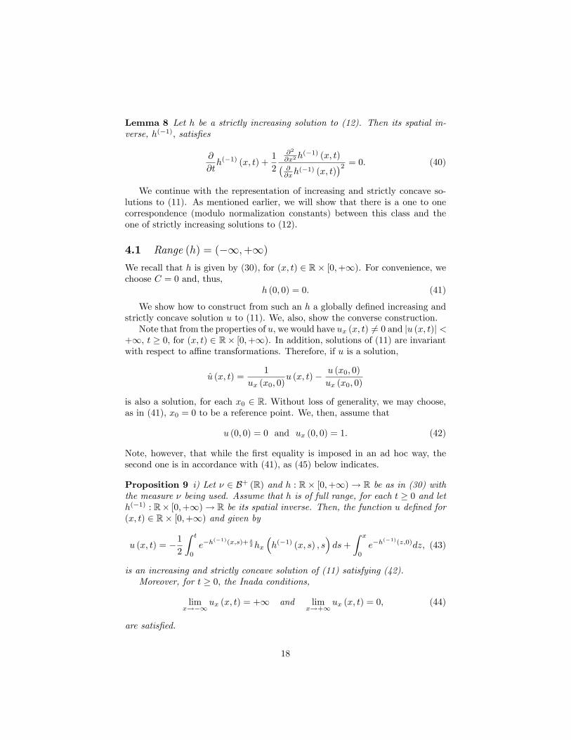
Lemma 8 Let h be a strictly increasing solution to (12). Then its spatial in-verse, h(�1); satis�es

@

@th(�1) (x; t) +

1

2

@2

@x2h(�1) (x; t)�

@@xh

(�1) (x; t)�2 = 0: (40)

We continue with the representation of increasing and strictly concave so-lutions to (11). As mentioned earlier, we will show that there is a one to onecorrespondence (modulo normalization constants) between this class and theone of strictly increasing solutions to (12).

4.1 Range (h) = (�1;+1)We recall that h is given by (30), for (x; t) 2 R� [0;+1). For convenience, wechoose C = 0 and, thus,

h (0; 0) = 0: (41)

We show how to construct from such an h a globally de�ned increasing andstrictly concave solution u to (11). We, also, show the converse construction.Note that from the properties of u; we would have ux (x; t) 6= 0 and ju (x; t)j <

+1; t � 0; for (x; t) 2 R� [0;+1). In addition, solutions of (11) are invariantwith respect to a¢ ne transformations. Therefore, if u is a solution,

u (x; t) =1

ux (x0; 0)u (x; t)� u (x0; 0)

ux (x0; 0)

is also a solution, for each x0 2 R: Without loss of generality, we may choose,as in (41), x0 = 0 to be a reference point. We, then, assume that

u (0; 0) = 0 and ux (0; 0) = 1: (42)

Note, however, that while the �rst equality is imposed in an ad hoc way, thesecond one is in accordance with (41), as (45) below indicates.

Proposition 9 i) Let � 2 B+ (R) and h : R� [0;+1)! R be as in (30) withthe measure � being used. Assume that h is of full range, for each t � 0 and leth(�1) : R� [0;+1)! R be its spatial inverse. Then, the function u de�ned for(x; t) 2 R� [0;+1) and given by

u (x; t) = �12

Z t

0

e�h(�1)(x;s)+ s

2hx

�h(�1) (x; s) ; s

�ds+

Z x

0

e�h(�1)(z;0)dz; (43)

is an increasing and strictly concave solution of (11) satisfying (42).Moreover, for t � 0; the Inada conditions,

limx!�1

ux (x; t) = +1 and limx!+1

ux (x; t) = 0; (44)

are satis�ed.

18

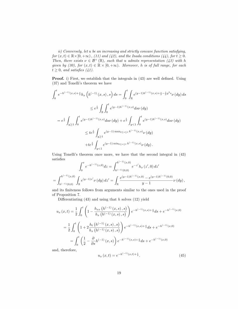
ii) Conversely, let u be an increasing and strictly concave function satisfying,for (x; t) 2 R�[0;+1) ; (11) and (42), and the Inada conditions (44), for t � 0.Then, there exists � 2 B+ (R), such that u admits representation (43) with hgiven by (30), for (x; t) 2 R � [0;+1). Moreover, h is of full range, for eacht � 0; and satis�es (41).

Proof. i) First, we establish that the integrals in (43) are well de�ned. Using(37) and Tonelli�s theorem we haveZ t

0

e�h(�1)(x;s)+ s

2hx

�h(�1) (x; s) ; s

�ds =

Z t

0

ZRe(y�1)h

(�1)(x;s)+ s2�

12y

2s� (dy) ds

� e t2ZR

Z t

0

e(y�1)h(�1)(x;s)ds� (dy)

= et2

Zy�1

Z t

0

e(y�1)h(�1)(x;s)ds� (dy) + e

t2

Zy<1

Z t

0

e(y�1)h(�1)(x;s)ds� (dy)

� te t2Zy�1

e(y�1)max0�s�t h(�1)(x;s)� (dy)

+tet2

Zy<1

e(y�1)min0�s�t h(�1)(x;s)� (dy) :

Using Tonelli�s theorem once more, we have that the second integral in (43)satis�es Z x

0

e�h(�1)(z;0)dz =

Z h(�1)(x;0)

h(�1)(0;0)

e�z0hx (z

0; 0) dz0

=

Z h(�1)(x;0)

h(�1)(0;0)

ZRe(y�1)z

0� (dy) dz0 =

ZR

e(y�1)h(�1)(x;0) � e(y�1)h(�1)(0;0)

y � 1 � (dy) ;

and its �niteness follows from arguments similar to the ones used in the proofof Proposition 7.Di¤erentiating (43) and using that h solves (12) yield

ux (x; t) =1

2

Z t

0

1�

hxx�h(�1) (x; s) ; s

�hx�h(�1) (x; s) ; s

� ! e�h(�1)(x;s)+ s2 ds+ e�h

(�1)(x;0)

=1

2

Z t

0

1 + 2

ht�h(�1) (x; s) ; s

�hx�h(�1) (x; s) ; s

�! e�h(�1)(x;s)+ s2 ds+ e�h

(�1)(x;0)

=

Z t

0

�1

2� @

@sh(�1) (x; s)

�e�h

(�1)(x;s)+ s2 ds+ e�h

(�1)(x;0)

and, therefore,ux (x; t) = e

�h(�1)(x;t)+ t2 : (45)

19

Further di¤erentiation yields

u2x (x; t)

uxx (x; t)= �e

�h(�1)(x;t)+ t2

@@xh

(�1) (x; t):

On the other hand, (43) implies

ut (x; t) = �1

2e�h

(�1)(x;t)+ t2hx

�h(�1) (x; t) ; t

�= �1

2

e�h(�1)(x;t)+ t

2

@@xh

(�1) (x; t):

Combining the above two equalities, we deduce that u satis�es (11).To establish (42) and (44), we �rst observe that the assumption of full range

yields, for each t � 0; limx!�1 h(�1) (x; t) = �1. Both assertions, then, follow

from (45).ii) Let u be an increasing and strictly concave function, de�ned for (x; t) 2

R � [0;+1) and satisfying (11), (42) and (44). Using that ux is invertible,with (ux)

(�1): (0;+1)� [0;+1)! R; we de�ne, for (x; t) 2 R� [0;+1) ; the

function h by

h (x; t) = (ux)(�1)

�e�x+

t2 ; t�: (46)

Note that h is invertible in the space variable since

hx (x; t) = �e�x+

t2

uxx (h (x; t) ; t)> 0:

Di¤erentiating (11) yields

uxt = ux �1

2

u2xuxxxu2xx

: (47)

In turn,

uxt (x; t) =

�� @@th(�1) (x; t) +

1

2

�ux (x; t) ;

uxx (x; t) = ��@

@xh(�1) (x; t)

�ux (x; t) (48)

and

uxxx (x; t) =

� @2

@x2h(�1) (x; t) +

�@

@xh(�1) (x; t)

�2!ux (x; t) :

Combining the above, we obtain that h(�1) satis�es

@

@th(�1) (x; t) +

1

2

@2

@x2h(�1) (x; t)�

@@xh

(�1) (x; t)�2 = 0;

20

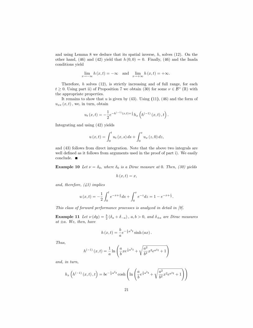
and using Lemma 8 we deduce that its spatial inverse, h; solves (12). On theother hand, (46) and (42) yield that h (0; 0) = 0. Finally, (46) and the Inadaconditions yield

limx!�1

h (x; t) = �1 and limx!+1

h (x; t) = +1:

Therefore, h solves (12), is strictly increasing and of full range, for eacht � 0: Using part ii) of Proposition 7 we obtain (30) for some � 2 B+ (R) withthe appropriate properties.It remains to show that u is given by (43). Using (11), (46) and the form of

uxx (x; t) ; we, in turn, obtain

ut (x; t) = �1

2e�h

(�1)(x;t)+ t2hx

�h(�1) (x; t) ; t

�:

Integrating and using (42) yields

u (x; t) =

Z t

0

ut (x; s) ds+

Z x

0

ux (z; 0) dz;

and (43) follows from direct integration. Note that the above two integrals arewell de�ned as it follows from arguments used in the proof of part i). We easilyconclude.

Example 10 Let � = �0; where �0 is a Dirac measure at 0: Then, (30) yields

h (x; t) = x;

and, therefore, (43) implies

u (x; t) = �12

Z t

0

e�x+s2 ds+

Z x

0

e�zdz = 1� e�x+ t2 :

This class of forward performance processes is analyzed in detail in [9].

Example 11 Let � (dy) = b2 (�a + ��a) ; a; b > 0; and ��a are Dirac measures

at �a: We, then, have

h (x; t) =b

ae�

12a

2t sinh (ax) :

Thus,

h(�1) (x; t) =1

aln

a

bxe

12a

2t +

ra2

b2x2ea2t + 1

!and, in turn,

hx

�h(�1) (x; t) ; t

�= be�

12a

2t cosh

ln

a

be12a

2t +

ra2

b2x2ea2t + 1

!!

21

=pa2x2 + b2e�a2t:

If, a = 1, then (43) yields

u (x; t) =1

2

�ln�x+

px2 + b2e�t

�� et

b2x�x�

px2 + b2e�t

�� t

2

�� 12ln b;

while, if a 6= 1;u (x; t)

=ap�

�2 � 1e1�a2 tb2e��t + a (1 + �)

��x2 + x

p�2x2 + b2e��2t

���x+

p�2x2 + b2e��2t

�1+ 1�

�ap�

�2 � 1b1� 1

a :

The involved calculations are cumbersome and, for this, omitted. A completedescription of this class of solutions can be found in [18].It is worth mentioning that the above functions provide an interesting exten-

sion of the traditional power and logarithmic utilities, mostly frequently used inportfolio choice. Note, however, that the latter utilities are not globally de�nedwhile the above are.

Example 12 Let � (dy) = 1p2�e�

12y

2

dy: Then,

h (x; t) = F

�xpt+ 1

�with F (x) =

Z x

0

e12 z

2

dz; x 2 R: (49)

Therefore, h(�1) (x; t) =pt+ 1F (�1) (x) and thus,

hx

�h(�1) (x; t) ; t

�=

1pt+ 1

f�F (�1) (x)

�; (50)

with f (x) = F 0 (x). Then, (43) becomes

u (x; t) = �12

Z t

0

1ps+ 1

f�F (�1) (x)

�e�

ps+1F (�1)(x)+ s

2 ds+

Z x

0

e�F(�1)(z)dz:

It turns out that

u (x; t) = k1F�F (�1) (x)�

pt+ 1

�+ k2 (51)

with k1 = e�12 and k2 = e�

12

R 0�1 e

12 z

2

dz:

The calculations are rather tedious but one can verify that u satis�es (42)and solves (43). Indeed,

ut (x; t) = �k1f�F (�1) (x)�

pt+ 1

�2pt+ 1

, ux (x; t) = k1f�F (�1) (x)�

pt+ 1

�f�F (�1) (x)

�22

and

uxx (x; t) = �k1pt+ 1

f�F (�1) (x)�

pt+ 1

��f�F (�1) (x)

��2 ;

and (11) follows. The equalities in (42) also follow from the form of u and thechoice of the constants k1; k2: Note, moreover, that the above yields

ux

�F

�xpt+ 1

�; t

�= e�x+

t2 ;

and (49) follows from (46).From (16) and (50), we deduce that the optimal policy of the above example

turns out to be��t =

1pAt + 1

f�F (�1) (X�

t )��+t �t; (52)

with At; t � 0; as in (13) and

X�t = F

�F (�1) (x) +At +Mtp

At + 1

�;

with the latter following from (15) and (49).We can see that the above measure, � (dy) = 1p

2�e�

12y

2

dy; violates condition(14) (for t > 0) and satis�es only (26). In turn, straightforward calculationsshow that ��t ; t � 0; is admissible but only in the local sense, i.e., ��t 2 Al but��t =2 A. We, then, deduce that the process Ut (x) = u (x;At) with u as in (51)satis�es De�nition 2, of a local forward performance process.

4.2 Range (h) = (x0;+1) ; x0 2 RWe recall that in this case, h is given by (30) where � satis�es

� 2 B++ (R) andZ +1

0+

� (dy)

y< +1; (53)

with B++ (R) given in (28). For convenience, we set in (30) C =R +10+

1y� (dy) ;

yielding5 Range (h) = (0;+1) ; as

h (x; t) =

Z +1

0+

eyx�12y

2t

y� (dy) : (54)

We can easily see, using the above and (11), that h is convex in its spatialargument and decreasing with regards to time,

hxx (x; t) > 0 and ht (x; t) < 0: (55)

5One may alternatively represent h as h (x; t) =R+10 eyx�

12y2t� (dy) with � (dy) = �(dy)

y:

Note that � 2 B+ (R) : Such a representation was used in [1].

23

Next, we obtain the analogous to (43) representation of the di¤erential inputu. As (43) shows, h plays the role of the space argument of u. Thus, thelatter is now de�ned on the half-line. Consideration then, needs, to be given tolimx!0 u (x; t) ; t � 0. The results below demonstrate that, depending on wherethe measure � is concentrated, this limit can be �nite or in�nite. In the lattercase, the monotonicity assumption yields that we must have limx!0 u (x; t) =�1; t � 0:

Proposition 13 i) Let � satisfy (53) and, in addition, � ((0; 1]) = 0: Let, also,h : R� [0;+1)! (0;+1) be as in (54) and h(�1) : (0;+1)� [0;+1)! R beits spatial inverse. Then, the function u de�ned, for (x; t) 2 (0;+1)� [0;+1) ;by

u (x; t) = �12

Z t

0

e�h(�1)(x;s)+ s

2hx

�h(�1) (x; s) ; s

�ds+

Z x

0

e�h(�1)(z;0)dz; (56)

is an increasing and strictly concave solution of (11) with

limx!0

u (x; t) = 0; for t � 0: (57)

Moreover, for t � 0; the Inada conditions

limx!0

ux (x; t) = +1 and limx!+1

ux (x; t) = 0 (58)

are satis�ed.ii) Conversely, let u, de�ned for (x; t) 2 (0;+1)� [0;+1) ; be an increasing

and strictly concave function satisfying (11), (57) and the Inada conditions (58).Then, there exists � 2 B+ (R) satisfying (53) and � ((0; 1]) = 0, such that uadmits representation (56) with h given by (54), for (x; t) 2 R� [0;+1) :

Proof. i) We �rst establish that u in (56) is well de�ned for x > 0; t � 0: From(54) and the assumptions on the measure �, we easily deduce that

hx (x; t) =

Z +1

1+eyx�

12y

2t� (dy) : (59)

Therefore, Z t

0

e�h(�1)(x;s)+ s

2hx

�h(�1) (x; s) ; s

�ds

=

Z t

0

Z +1

1+e(y�1)h

(�1)(x;s)+ s2�

12y

2s� (dy) ds:

Using that hx (x; t) � 0 and (55), we deduce that @@th

(�1) (x; t) � 0: The aboveequality then yieldsZ t

0

e�h(�1)(x;s)+ s

2hx

�h(�1) (x; s) ; s

�ds � te�h

(�1)(x;0)+ t2

Z +1

1+eyh

(�1)(x;t)� (dy) ;

24

and the �niteness of the integral follows easily from the assumptions on themeasure �:The �niteness of the second integral in (56) also follows. Indeed, �rst observe

that (54) yields

limx!�1

h (x; t) = 0 and limx!+1

h (x; t) = +1: (60)

Using the above, (59) and Tonelli�s theorem, we obtainZ x

0

e�h(�1)(z;0)dz =

Z h(�1)(x;0)

�1e�z

0hx (z

0; 0) dz0

=

Z h(�1)(x;0)

�1

Z +1

1+e(y�1)z

0� (dy) dz0 =

Z +1

1+

Z h(�1)(x;0)

�1e(y�1)z

0dz0� (dy)

=

Z +1

1+

1

y � 1

�e(y�1)h

(�1)(x;0) � limz0!�1

e(y�1)z0�� (dy)

=

Z +1

1+

1

y � 1e(y�1)h(�1)(x;0)� (dy) : (61)

For " > 0; we then haveZ x

0

e�h(�1)(z;0)dz =

Z 1+"

1+

1

y � 1e(y�1)h(�1)(x;0)� (dy)

+

Z +1

1+"

1

y � 1e(y�1)h(�1)(x;0)� (dy)

� max�1; e"h

(�1)(x;0)�Z 1+"

1+

� (dy)

y � 1 +e�h

(�1)(x;0)

"

Z +1

1+"

eyh(�1)(x;0)� (dy) ;

and the �niteness of the above terms follows from the assumptions on the mea-sure � and the monotonicity of the function 1

y�1 (y 6= 1) :The fact that u solves (11) and has the claimed monotonicity and concavity

properties follows from arguments similar to the ones used in the proof of parti) in Proposition 9.Next, we establish (57). We claim that

limx!0

Z t

0

e�h(�1)(x;s)+ s

2hx

�h(�1) (x; s) ; s

�ds = 0: (62)

Indeed, note that the above integrand is monotone in x: This follows easily fromits representation,

e�h(�1)(x;t)+ t

2hx

�h(�1) (x; t) ; t

�=

Z +1

1+e(y�1)h

(�1)(x;t)� 12y

2t+ t2 � (dy) ;

25

combined with the monotonicity of h(�1): Using the monotone convergence the-orem and (60), we obtain (62).To show

limx!0

Z x

0

e�h(�1)(z;0)dz = 0

we use (61), the monotone convergence theorem and (60) (for t = 0):ii) Using arguments similar to the ones in the proof of part ii) in Proposition

9, we deduce that the function h given, for (x; t) 2 R� [0;+1) ; by

h (x; t) = (ux)(�1)

�e�x+

t2 ; t�

(63)

is well de�ned and solves (12). Moreover, the assumptions on u imply thath (x; t) � 0 and hx (x; t) � 0: Therefore, from Proposition 7, we have that thereexists � 2 B+ (R) satisfying (53) and such that representation (54) holds. TheInada conditions (58) then yield that the normalization constant must be chosenas C =

R +10+

1y� (dy).

Using (57) and working along similar arguments used in the proof of Propo-sition 7, we deduce the representation (56).It remains to establish that � ((0; 1]) = 0: We argue by contradiction. To

this end, we �rst note that because of (57), we have, for x > 0;

u (x; t) =

Z x

0

ux (z; t) dz =

Z h(�1)(x;t)

�1

Z +1

0

e(y�1)z0+ t

2 (1�y2)� (dy) dz0;

where we used (46) and (60). We, then, observe that � cannot include a Diracmeasure at y = 1 as this would yield

u (x; t) �Z h(�1)(x;t)

�1dz0 = +1;

contradicting the �niteness of u (x; t) : Therefore, we must have

u (x; t) =

Z h(�1)(x;t)

�1

Z 1�

0+e(y�1)z

0+ t2 (1�y

2)� (dy) dz0

+

Z h(�1)(x;t)

�1

Z +1

1+e(y�1)z

0+ t2 (1�y

2)� (dy) dz0:

On the other hand, using the above and Tonelli�s theorem, we deduce, for x > 0;

u (x; t) �Z h(�1)(x;t)

�1

Z 1�

0+e(y�1)z

0+ t2 (1�y

2)� (dy) dz0

�Z 1�

0+

Z h(�1)(x;t)

�1e(y�1)z

0+ t2 (1�y

2)dz0� (dy)

26

=

Z 1�

0+

1

y � 1

�e(y�1)h

(�1)(x;t) � limz!�1

e(y�1)z0�� (dy) ;

and we easily get a contradiction to (57).Working along similar arguments we obtain the following result.

Proposition 14 i) Let � satisfy (53) and, in addition, � ((0; 1]) > 0: Let, also,h : R� [0;+1)! (0;+1) be as in (54) and h(�1) : (0;+1)� [0;+1)! R beits spatial inverse. Then, the function u de�ned, for (x; t) 2 (0;+1)� [0;+1) ;by

u (x; t) = �12

Z t

0

e�h(�1)(x;s)+ s

2hx

�h(�1) (x; s) ; s

�ds+

Z x

x0

e�h(�1)(z;0)dz; (64)

for x0 > 0; is an increasing and strictly concave solution of (11) with

limx!0

u (x; t) = �1; for t � 0: (65)

Moreover, for each t � 0; the Inada conditions

limx!0

ux (x; t) = +1 and limx!+1

ux (x; t) = 0 (66)

are satis�ed.ii) Conversely, let u; de�ned for (x; t) 2 (0;+1)� [0;+1) ; be an increasing

and strictly concave function satisfying (11), (65) and the Inada conditions (66).Then, there exists � 2 B+ (R) satisfying (53) and � ((0; 1]) > 0, such that uadmits representation (64) with h given, for (x; t) 2 R� [0;+1) ; by (54).

Example 15 Let � = � ; > 1: Then, (54) yields

h (x; t) =1

e x�

12

2t;

for (x; t) 2 R � [0;+1) : We, then, have h(�1) (x; t) = ln ( x)1 + 1

2 t; (x; t) 2(0;+1)� [0;+1) and, thus, hx

�h(�1) (x; t) ; t

�= x:

Since � ((0; 1]) = 0; u is given by (56) and, therefore,

u (x; t) = �12

Z t

0

xe��ln( x)

1 + 1

2 s

�+ s2ds+

Z x

0

( z)� 1 dz

= �1

� 1x �1 e�

�12 t:

Example 16 Let � = � ; = 1: Then, (54) yields

h (x; t) = ex�12 t;

for (x; t) 2 R � [0;+1) : We, then, have h(�1) (x; t) = lnx + 12 t; (x; t) 2

(0;+1)� [0;+1) and, thus, hx�h(�1) (x; t) ; t

�= x:

27

Since � ((0; 1]) 6= 0; u is given by (64). Therefore, for (x; t) 2 (0;+1) �[0;+1) and x0 > 0;

u (x; t) = �12

Z t

0

xe�(ln x+12 s)+

s2 ds+

Z x

x0

1

zdz = ln

x

x0� t

2:

Example 17 Let � = � ; 2 (0; 1) : Using Example 15 and that � ((0; 1]) 6= 0;we easily deduce, using (65), that u is given by

u (x; t) = �12

Z t

0

xe��ln( x)

1 +

2 s

�+ s2ds+

Z x

x0

( z)� 1 dz

= � �1

1� x �1 e

1� 2 t +

�1

1� x �1

0 ;

for x0 > 0:

4.3 Range(h) = (�1; x0) ; x0 2 RWe recall that in this case, h is given by (30) where � satis�es

� 2 B+� (R) andZ 0�

�1

� (dy)

y> �1; (67)

with B+� (R) given in (29). For convenience, we set in (30) C =R 0��1

�(dy)y ;

yielding Range(h) = (�1; 0) ; as

h (x; t) =

Z 0�

�1

eyx�12y

2t

y� (dy) : (68)

In analogy to (55), one can show that h is concave in its spatial argument andincreasing with regards to time,

hxx (x; t) < 0 and ht (x; t) > 0: (69)

The next proposition follows from a modi�cation of the arguments used toprove Proposition 14.

Proposition 18 i) Let � be as in (67). Let, also, h : R � [0;+1) ! (�1; 0)be as in (68) and h(�1) : (�1; 0)� [0;+1)! R be its spatial inverse. Then,the function u de�ned, for (x; t) 2 (�1; 0)� [0;+1) ; by

u (x; t) = �12

Z t

0

e�h(�1)(x;s)+ s

2hx

�h(�1) (x; s) ; s

�ds�

Z 0

x

e�h(�1)(z;0)dz; (70)

is an increasing and strictly concave solution of (11) with

limx!0

u (x; t) = 0; for t � 0: (71)

28

Moreover, for each t � 0; the Inada conditions

limx!�1

ux (x; t) = +1 and limx!0

ux (x; t) = 0 (72)

are satis�ed.ii) Conversely, let u be an increasing and strictly concave function satisfying,

for (x; t) 2 (�1; 0) � [0;+1) ; (11), (71) and the Inada conditions (72), fort � 0. Then, there exists � as in (67) such that u admits representation (70)with h given by (68).

Example 19 We take � = � ; = � 12k+1 ; k > 0: Then, (68) yields, for

(x; t) 2 (�1; 0)� [0;+1) ;

h (x; t) = � 1 e x�

12

2t:

Working as in Example 15, we deduce that, for (x; t) 2 (�1; 0)� [0;+1) ;

u (x; t) = �1

� 1x �1 e�

�12 t = � (2k + 1)

�2k�1

2 (k + 1)x2(k+1)e

k+12k+1 t:

4.4 Range(h) = (x1; x2) ; x1; x2 2 RThe case of �nite range is not considered since it does not yield a meaningfulsolution. Indeed, we recall the following result derived by Widder (see [17]).

Proposition 20 Let h be a solution to (12) such that for (x; t) 2 R� [0;1) ;�M � h (x; t) �M; for some constant M: Then, h (x; t) is constant.

It, then, easily follows that in this case the problem degenerates as there isno strictly increasing solution to (12) and, in turn to (11).

4.5 The local risk tolerance

In section 3, we introduced the function r in (22). This function facilitatesthe representation of the optimal portfolio policy (cf. (23)) and, as it is shownbelow, is represented in terms of the spatial derivatives of u. In the traditionalmaximal expected utility models, a similar quantity is used, known as the risktolerance. We keep an analogous terminology herein.For the generic spatial domain D appearing below, we have D = R; (0;+1)

or (�1; 0) : To ease the presentation, we omit any reference to the speci�c rangeh (and, thus, to the domain of u):The following result is a direct consequence of (22) and (46) (for an alterna-

tive proof, see [10]).

Proposition 21 Let r : D� [0;1)! (0;+1) be given by (22), i.e.

r (x; t) = hx

�h(�1) (x; t) ; t

�; (73)

29

and u be the associated with h di¤erential utility input. Then, for (x; t) 2D� [0;1) ;

r (x; t) = � ux (x; t)uxx (x; t)

:

In (25) we saw that the monotonicity of the optimal investment strategywith regards to the initial endowment depends directly on the sign of the partialderivative rx (x; t) : As it was mentioned in section 3, when the risk toleranceis de�ned on R � [0;+1) very little, if anything, can be established for itsmonotonicity or limiting behavior. When, however, its domain is semi-in�nite,we have the following results.

Proposition 22 Let r : D� [0;+1)! (0;+1) with D =(0;+1) or (�1; 0) :Then, for t � 0;

limx!0

r (x; t) = 0: (74)

If D =(0;+1) ; thenrx (x; t) � 0; (75)

while, if D =(�1; 0),rx (x; t) � 0; (76)

for t � 0:

Proof. We only establish (74) when D =(0;+1) : Recalling that

hx (x; t) =

Z +1

0+eyx�

12y

2t� (dy)

(cf. (54)), (73) yields

r (x; t) =

Z 1

0+eyh

(�1)(x;t)� 12y

2t� (dy) :

Passing to the limit, and using the monotone convergence theorem and (60), weconclude.Next, we show (75). Di¤erentiating (73) yields

rx (x; t) =

�@

@xh(�1) (x; t)

�hxx

�h(�1) (x; t) ; t

�:

When D =(0;+1) (resp. D =(�1; 0)); then (75) (resp. (76)) follows from(55) (resp. (69)).

5 Deterministic market prices of risk

In this section we assume that the process �t; t � 0; (cf. (3)) is determin-istic. The goal is twofold. Firstly, we study distributional properties of theoptimal wealth and compute its cumulative distribution, density and moments.Secondly, we explore some inverse problems, namely, how could the investor�spreferences be inferred from information about the targeted mean of his optimalwealth.

30

5.1 Distribution of the optimal wealth process

Recalling At and Mt from (13) we have hMit = At; t � 0; and, thus, by Levy�stheorem the process Mt is a Gaussian martingale. This leads to the followingproperties of the distribution of the investor�s optimal wealth process. Thefunctions N and n below stand, respectively, for the cumulative distributionand the density functions of a standard normal variable. We recall that h solves(12), h(�1) stands for its spatial inverse and r is given in (22).

Proposition 23 i) The cumulative distribution and probability density func-tions of the optimal wealth X�;x

t ; t > 0; are given, respectively, by

P�X�;xt � y

�= N

�h(�1) (y;At)� h(�1) (x; 0)�Atp

At

�(77)

and

fX�;xt(y) = n

�h(�1) (y;At)� h(�1) (x; 0)�Atp

At

�1

r (y;At)pAt;

with At as in (13).ii) For all p 2 [0; 1] and t > 0; the quantile of order p, i.e. the point yp (t)

for which P�X�;xt � yp (t)

�= p; is given by

yp (t) = h�h(�1) (x; 0) +At +

pAtN

(�1) (p) ; At

�:

Proof. The �rst statement follows directly from (15). Indeed,

P�X�;xt � y

�= P

�h�h(�1) (x; 0) +At +Mt; At

�� y�

= P�h(�1) (x; 0) +At +Mt � h(�1) (y;At)

�;

and we easily conclude. The other two statements are also immediate.Properties of the multivariate distributions may be analyzed along similar

arguments.

Next, we study the expected value of the optimal wealth and portfolioprocesses.

Proposition 24 Let X�;xt and ��;xt be as in (15) and (16). Then, for t > 0;

E�X�;xt

�= h

�h(�1) (x; 0) +At; 0

�: (78)

Moreover,@

@xE�X�;xt

�=r�E�X�;xt

�; 0�

r (x; 0)(79)

andE�r�X�;xt ; At

��= r

�E�X�;xt

�; 0�: (80)

31

Proof. We establish the above when the function h is as in (30), with the othercases, exhibited in (54) and (68), following along similar arguments.From (15) we have

E�X�;xt

�= E

�h�h(�1) (x; 0) +At +Mt; At

��= E

ZR

ey(h(�1)(x;0)+At+Mt)� 1

2y2At � 1

y� (dy)

!

=

ZRE

ey(h

(�1)(x;0)+At+Mt)� 12y

2At � 1y

!� (dy)

=

ZR

ey(h(�1)(x;0)+At) � 1

y� (dy) = h

�h(�1) (x; 0) +At; 0

�:

Above we used that the two integrals can be interchanged. For this, it su¢ cesto have

E

ZR

�����ey(h(�1)(x;0)+At+Mt)� 1

2y2At � 1

y

����� � (dy)!< +1: (81)

Indeed, inequality (32) yieldsZR

�����eyx�12y

2t � 1y

����� � (dy) � � (R)�ex+ t2 + e�x+

t2

�+

ZReyx�

12y

2t� (dy) :

Therefore,

E

ZR

�����ey(h(�1)(x;0)+At+Mt)� 1

2y2At � 1

y

����� � (dy)!

� � (R)E�eh

(�1)(x;0)+At+Mt+At2 + e�(h

(�1)(x;0)+At+Mt)+At2

�+E

�ZRey(h

(�1)(x;0)+At+Mt)� 12y

2At� (dy)

�:

On the other hand,

E�eh

(�1)(x;0)+At+Mt+At2 + e�(h

(�1)(x;0)+At+Mt)+At2

�� e

h(�1)(x;0)+ 32c2t

E�eMt

�+ e�h

(�1)(x;0);

where we used (5) and (13). Similarly,

E

�ZRey(h

(�1)(x;0)+At+Mt)� 12y

2At� (dy)

�

=

ZRE�ey(h

(�1)(x;0)+At+Mt)� 12y

2At

�� (dy)

32

=

ZRey(h

(�1)(x;0)+At)� (dy) <

ZRey(h

(�1)(x;0)+c2t)� (dy) < +1;

and we easily obtain (81). Assertion (79) follows from (78) and (22).To show (80), we recall (15), (22) and (34) yielding

E�r�X�;xt ; At

��= E

�ZRey(h

(�1)(x;0)+At+Mt)� 12y

2At� (dy)

�

=

ZRey(h

(�1)(x;0)+At)� (dy) = hx

�h(�1) (x; 0) +At; 0

�;

and we easily conclude.

5.2 Inferring the investor�s preferences

The investment performance criterion (19) combines the investor�s preferenceswith the market input. As a consequence, the optimal portfolio and the associ-ated wealth (see (16) and (15), respectively) contain implicit information aboutthese preferences. In this section, we discuss how to learn about the individual�srisk attitude by analyzing distributional characteristics of his optimal wealth.One can say, using the language of the derivatives industry, that our aim is tocalibrate the investor�s preferences, given the market dynamics and his desirabledistributional outcomes for his wealth process.This idea is relatively new. To the best of our knowledge, the authors of [15]

were the �rst to propose a model and show how information about an investor�smarginal utility of wealth can be inferred from her choice of a distribution.Other, more recent relevant references, are [2] and [16].We discuss two examples in which we infer the investor�s preferences using

information about the behavior of her average future wealth. For simplicity, weonly concentrate on the no-bankruptcy case, Range(h) = (0;+1) (see section4.2).

Proposition 25 Let the mapping x ! E�X�;xt

�be linear, for all x > 0 and

t � 0. Then, there exists a positive constant > 0 such that the investor�sforward performance process is given by

Ut (x) = �1

� 1x �1 e�

12 ( �1)At ; (82)

if 6= 1 and byUt (x) = lnx�

1

2At; (83)

if = 1: Moreover,E�X�;xt

�= xe At : (84)

33

Proof. Di¤erentiating (79) we deduce

@2

@x2E�X�;xt

�=rx�E�X�;xt

�; 0�

r (x; 0)

@

@xE�X�;xt

�� r

�E�X�;xt

�; 0� rx (x; 0)r2 (x; 0)

=

�rx�E�X�;xt

�; 0�� rx (x; 0)

�r2 (x; 0)

r�E�X�;xt

�; 0�:

By assumption @2

@x2E�X�;xt

�= 0: Moreover, r

�E�X�;xt

�; 0�> 0 as it follows

from (80). Therefore, we must have

rx�E�X�;xt

�; 0�= rx (x; 0)

and, in turn,

@

@trx�E�X�;xt

�; 0�= rxx

�E�X�;xt

�; 0� @@tE�X�;xt

�= 0:

However, (78) implies @@tE

�X�;xt

�6= 0 and, thus, we deduce that

rxx�E�X�;xt

�; 0�= 0:

Therefore, the function r (x; 0) must be linear in E�X�;xt

�and, in turn, in x,

per our assumption. Using (74) we obtain

r (x; 0) = x;

for some > 0: From (22) and (54) we, then, deduce that for all x > 0;Z +1

0+eyh

(�1)(x;0)� (dy) = x

and, in turn, Z +1

0+eyx� (dy) =

Z +1

0+

eyx

y� (dy) :

Therefore, we must have� (dy) = �

where � is a Dirac measure at > 0: This yields

h (x; t) =1

e x�

12

2t

and assertions (82) and (83) follow from Examples 15, 16 and 17.Equality (84) follows from (78) and the form of h:

From the above analysis, we see that calibrating the investor�s preferencesconsists of choosing a time horizon and the level of the mean of her optimal

34

wealth, say t0 and mx (m > 1), respectively. Then, (84) implies that thecorresponding must satisfy xe At0 = mx, or, equivalently,

=lnm

At0:

Note that under the linearity assumption, the investor can calibrate her ex-pectations only for a single time horizon. The model interpolates for all othertrading horizons, giving

E (X�xt ) = xm

AtAt0 :

We easily deduce that the distribution of the optimal wealth X�;xt is lognormal,

for all (x; t) :

The linearity of the mapping x ! E�X�;xt

�is a very strong assumption.

Indeed, it only allows for calibration of a single parameter, namely, the slope,and, moreover, for a single time horizon. Therefore, if one intends to calibratethe investor�s preferences to more re�ned information, then one needs to accepta more complicated dependence of E

�X�;xt

�on x: We discuss this case next.

To this end, let us �x the level of initial wealth at x = 1 and consider

calibration to E�X�;1t

�; for t > 0. The investor then chooses an increasing

function m (t) (with m (t) > 1) to represent the latter, i.e. for t > 0;

E�X�;1t

�= m (t) : (85)

What does this choice reveal about her preferences? Moreover, can she choose anarbitrary increasing function m (t)? We give answers to these questions below.In analogy to the previous proposition, we only consider the no bankruptcy

case, which corresponds to h given in (54). Using arguments similar to theones used in Proposition 6, we may assume, without loss of generality, thatR +10

�(dy)y = 1: We, then, have h(�1) (1; 0) = 0 which, combined with (78),

yields

E�X�;1t

�= h (At; 0) =

Z 1

0+

eyAt

y� (dy) :

We easily see that the investor may only choose a function m (t) ; t � 0; whichcan be represented in the form

m (t) =

Z 1

0+

eyAt

y� (dy) : (86)

Therefore, the choice of a feasible m (t) reduces to the choice of the appropriatemeasure �: Speci�cally, we must have,

m�A(�1)t

�=

Z 1

0+

eyt

y� (dy) = h (t; 0) ; (87)

35

where A(�1)t stands for the inverse of the process At; t � 0: Note that the righthand side above is the moment generating function of the probability measure� (dy) = �(dy)

y :

Assume now that the mean m (t) (cf. (85)) was chosen so that (87) holdsfor some measure �: Then, for other values of x > 0; x 6= 1; we have, using (78),

E�X�;xt

�= m

�A(�1)

�h(�1) (x; 0) +A (t)

��= m

�A(�1)

�A�m(�1) (x)

�+A (t)

��;

where, for notational convenience, At (resp. A(�1)t ) is denoted by A(t) (resp.

A(�1)(t)):In summary, the market related input At; coupled with the investor�s tar-

geted mean m (t) (at initial wealth x = 1); yields the investor�s preferences bychoosing the measure �; appearing in (86). Note that the process At determinesthe distribution of the martingale Mt and the measure � de�nes the functionh; which, in turn, determines the functions u and r: Once these quantities arespeci�ed, we are able to construct the optimal portfolio process that generatesthe optimal wealth which satis�es (85). The distribution of the optimal wealthprocess X�;x

t ; for x > 0; x 6= 1; is, in turn, deduced from the speci�cation of thetargeted mean, m (t) ; the market input At and (77).We conclude mentioning that one may prefer to calibrate the distribution of

the optimal wealth at a given time, say, X�;1t0 ; rather than the mean, E

�X�;1t

�;

for t � 0: It is easy to see what distributions are attainable. Indeed, Proposition23 would give

P�X�;1t0 � y

�= N

h(�1) (y;At0)�At0p

At0

!with

h (y;At0) =

Z 1

0+

ezy�12 z

2At0

y� (dz) :

Further analysis of this and other calibration issues is left for future research.

References

[1] Barrier F., Rogers L.C. and M. Tehranchi: A characterization of forwardutility functions, preprint, (2007).

[2] Goldstein, D.G., Johnson E.J. and W.F. Sharpe: Measuring consumer risk-return trade-o¤s, preprint (2006).

[3] Hu, Y. and X.Y. Zhou: Constrained stochastic LQ control with randomcoe¢ cients, and application to mean�variance portfolio selection, SIAMJournal on Control and Optimization, 44, 444-466 (2005).

36

[4] Jin, H. and X.Y. Zhou: Behavioral portfolio selection in continuous time,Mathematical Finance, 18, 385-426 (2008).

[5] Karatzas, I. and G. Zitkovic: Optimal consumption from investment andrandom endowment in incomplete semimartingale markets, Annals of Ap-plied Probability, 31(4), 1821-1858 (2003).

[6] Li, X. and X.Y. Zhou: Continuous-time mean�variance e¢ ciency: The 80%rule", Annals of Applied Probability, 16, 1751-1763 (2006).

[7] Lipster, R.S. and A.N. Shiryaev: Statistics of Random Processes, II : Ap-plications (2nd edition), Springer, Berlin (2000).

[8] Merton, R. : Lifetime portfolio selection under uncertainty: the continuous-time case, The Review of Economics and Statistics, 51, 247-257 (1969).

[9] Musiela, M. and Zariphopoulou, T.: Optimal asset allocation under forwardexponential criteria, Markov Processes and Related Topics: A Festschriftfor Thomas. G. Kurtz, IMS Collections, Institute of Mathematical Statis-tics, 4, 285-300 (2008).

[10] Musiela, M. and T. Zariphopoulou: Portfolio choice under dynamic invest-ment performance criteria, Quantitative Finance, in print.

[11] Musiela, M. and T. Zariphopoulou: Stochastic partial di¤erential equationsin portfolio choice, preprint (2007).

[12] Musiela, M. and T. Zariphopoulou: Investments and forward utilities,preprint (2006).

[13] Penrose, R.: A generalized inverse for matrices, Proceedings of CambridgePhilosophical Society, 51, 406-413 (1955).

[14] Schachermayer, W.: A Super-Martingale Property of the Optimal PortfolioProcess, Finance and Stochastics, 7, 433-456 (2003).

[15] Sharpe W.F., Goldstein D.G. and P.W. Blythe: The distribution builder:A tool for inferring investor�s preferences, preprint (2000).

[16] Sharpe W.F.: Expected utility asset allocation, preprint (2006).

[17] Widder, D.V.: The heat equation, Academic Press (1975).

[18] Zariphopoulou, T. and T. Zhou: Investment performance measurementunder asymptotically linear local risk tolerance, Handbook of NumericalAnalysis, A. Bensoussan (Ed.), in print (2007).

[19] Zitkovic, G.: A dual characterization of self-generation and log-a¢ ne for-ward performances, submitted for publication (2008).

37