1

Investment Management

Portfolio Analysis and Diversification

Road Map

• Capital allocation (single risky asset)• Capital allocation (multiple assets)• Portfolio diversification• Mean-variance principle• Efficient frontier and optimal portfolios• Passive portfolio management• Who is the generic investor?

2

Capital allocation

• Portfolio managers seek to achieve the best possible trade-off between risk and return.

• How much to invest between the risky investments (high-risk/high return) and a risk-free investment?

• Capital allocation ≠ asset allocation (i.e. composition on risky assets) ≠ security allocation decision (i.e. security selection within each asset class)

Example: one risky asset

• Assume that the total market value of an initial portfolio is $300,000 of which:

– $90,000 is invested in a money market fund

– $210,000 is invested in equities

• The weight of the risky portfolio p within the optimal (complete) portfolio, i.e. including risky and risk-free assets, is

210,0000.7 (or 70%)

300,000

90,0001 0.3 (or 30%)

300,000

= =

− = =

y

y

3

Example: one risky asset

• A portfolio manager has to decide how much (which proportion y of wealth) to invest in a risky (diversified) portfolio and the risk-free asset

• Assume that E(Rp) is the expected return of the risky portfolio

and σp is its associated risk. The risk-free return is rf. The expected return of the resulting complete portfolio is

and its risk equals

( ) ( ) ( )

( )= + − =

⎡ ⎤= + −⎣ ⎦

1C p f

f p f

E r yE r y r

r y E r r

σ = σC py

Example: one risky asset (cont’d)

Let E(Rp) = 15%, σp= 22% and rf = 7%

100% risky asset

100% risk-free asset

4

Capital allocation line

• We can define the Capital allocation line (CAL) as follows:

• The quantity is called reward-to-

variability ratio (or Sharpe ratio), hence

• CAL is a straight line describing the possible

risk/return combinations available to investors.

( ) ( ) ( )⎡ ⎤−⎣ ⎦⎡ ⎤= + − = + σ⎣ ⎦ σp f

C f p f f C

p

E r rE r r y E r r r

( )⎡ ⎤= − σ⎣ ⎦/p f pS E r r

( ) = + σC f CE r r S

Leverage

• Suppose that the initial investment budget is $300,000 but the investor borrows additional funds for $120,000 to invest the total amount in the risky asset.

• This is called leveraged position in in the risky asset

• A negative number denotes a short position

– short position in the risk-free asset = borrowing

– short position in the risky asset = short selling

420,0001.4 (or 140%)

300,000

1 1 1.4 0.4

= =

− = − = −

y

y

5

Risk aversion and optimal portfolios

• CAL describes all feasible alternatives available to investors, however which is one is the most suitable? Put differently, how can we select the optimal portfolio for a generic investor?

• This entails the explicit consideration of investors’ risk aversion and their utility levels

• Recall U = E(r) – 1/2Aσ2 and

( ) ( )⎡ ⎤= + −⎣ ⎦σ = σ → σ = σ2 2 2

C f p f

C p C p

E r r y E r r

y y

Risk aversion and optimal portfolios (cont’d)

• Investor will choose their fraction to allocate to the risky portfolio y by maximising their utility (given their attitude towards risk, or risk aversion A):

• The resulting optimal allocation y* is

( )⎡ ⎤= + − − σ⎣ ⎦2 2max 1 2f p f p

yU r y E r r Ay

( )( )

= − σ =

⎡ ⎤= + − − σ⎣ ⎦

2

2 2

1 2

1 2

C C

f p f p

U E r A

r y E r r Ay

( ) −=

σ*

2

p f

p

E r ry

A

6

Risk aversion and optimal portfolios (cont’d)

Risk aversion and optimal portfolios (cont’d)

7

Risk aversion and optimal portfolios (cont’d)

• Assume that A = 4, hence

• when 41% is invested in the risky asset the optimal (complete) portfolio will exhibit

−= =

×− =

*

2

*

0.15 0.070.41

4 0.22

1 0.59

y

y

( ) ( )= + × − =

σ = × =

0.07 0.41 0.15 0.07 0.1028%

0.41 0.22 0.0902%

C

C

E r

Recall: how do individuals invest?

• Passive management

– “buy and hold” a well-diversified portfolio of assets

• Active management

– security selection attempts to identify securities that have been mispriced - e.g. “buy low and sell high”

– market timing tilts the portfolio composition in favour of (away from) equities when the investor is bullish (bearish) about the stock market

• Portfolio insurance

– use derivative securities to “manage” risk

8

Passive portfolio strategy

• A passive strategy describes a portfolio decision which does not engage in any direct or indirect security analysis

• If we substitute in our previous example the diversified portfolio p with the market portfolio (i.e. a well diversified portfolio of common stocks that mirrors the value of the corporate sector of a certain economy, S&P 500, FTSE 100, HSI, NIKKEI 225 etc.) we obtain the Capital market line (CML)

Passive portfolio strategy (cont’d)

• How reasonable is a passive strategy for an investor?

– alternative strategies (i.e. active) are not free

– free-riding benefits (asset are in general fairly priced, EMH)

• A passive portfolio strategy implies

( ) −=

σ*

2

M fpassive

M

E r ry

A

9

Example: multiple risky assets

• In the previous example a portfolio manager was given a fully diversified portfolio and a risk-free asset

• However, how can we construct fully diversified, efficientportfolios of multiple risky assets? Does the asset allocation process change?

• In order to understand the formation of efficient portfolios of multiple risky asset, we need to investigate the ‘power’ of diversification

Preliminary: portfolio definitions

• Portfolio p constructed from n assets

– asset i has expected return E(ri)

– return on asset i has variance σ2i

– covariance of returns on assets i and j is cov(ri,rj)

• Portfolio weights w1, w2, .., wn with ∑wi ≡ 1 for i=1,2, ..,n

• Expected return and variance on portfolio p:

( ) ( )

( ) ( )2 2cov , with cov ,

p i ii

p i j i j i i ii j

E r w E r

w w r r r rσ σ

=

= =

∑

∑∑

10

Portfolio diversification

• Assume that

– expected return E(ri) = μ– variance of returns σ2

i = v

– covariance of returns cov(ri,rj) = c

• Equally-weighted portfolio, that is wi = 1/n for i=1,2, ..,n

• Expected return and variance on portfolio p:

( ) ( )

( )2

1

1cov , 1

p i ii

p i j i ji j

E r w E r nn

vw w r r cn n

μ μ

σ

⎛ ⎞= = =⎜ ⎟⎝ ⎠

⎛ ⎞= = + −⎜ ⎟⎝ ⎠

∑

∑∑

Portfolio diversification (cont’d)

• Diversification can eliminate specific risk:

1. n = 1 E(rp) = μ σ2p = v

2. n → ∞ E(rp) = μ σ2p = c

• Spread wealth over infinite number of assets

– expected return unchanged

– variance reduction

• Problems with holding an infinite number of assets?

2 11pv cn n

σ ⎛ ⎞= + −⎜ ⎟⎝ ⎠

11

Portfolio diversification (cont’d)

Portfolio diversification (cont’d)

12

Diversification and efficiency

• Diversification allows investor to reduce the level of the overall risk of a portfolio by eliminating the impact of individual/idiosyncratic risk

• Naïve diversification is not necessarily efficient

• Efficiently diversified portfolios are those which provide the lowest possible risk for any level of expected return (or the highest return for any level of risk)

• Efficiency is strictly related with the covariance of (expected) asset returns

Efficient frontier with 2 risky assets

• The efficient frontier is the combination of efficient portfolio expected returns and standard deviations that can be constructed out of the (two) available assets– If the covariance term is negative the overall risk is reduced

– If the covariance term is positive (but asset returns are less than perfectly positively correlated, ρ ≠ 1) there is still reduction in the overall risk

– With asset returns perfectly negatively correlated (i.e. ρ = −1) a perfectly hedged position (=zero risk) can be achieved

( ) ( ) ( )( )

1 1 2 2

2 2 2 2 21 1 2 2 1 2 1 2

2 2 2 21 1 2 2 1 2 1 2 1,2

2 cov ,

2

p

p

E r w E r w E r

w w w w r r

w w w w

σ σ σ

σ σ σ σ ρ

= +

= + + =

= + +

13

Efficient frontier with 2 risky assets

Asset allocation with risk-free asset and multiple risky assets

• Differently from the first example (only one risky asset), here we have a case where there are multiple risky assets and a risk-free asset

• How can we optimally combine them?

– Step 1: find the efficient frontier implied by the return/risk characteristics of the n risky asset classes

– Step 2: calculate the composition and return/risk characteristics of the tangency portfolio (maximizes the slope of the line from the risk-free asset to the efficient frontier)

– Step 3: calculate the composition and return/risk characteristics of the optimal portfolio (unique combination of the risk-free asset and the tangency portfolio which maximizes the expected utility of the investor’s end-of-period wealth)

14

… in diagrams

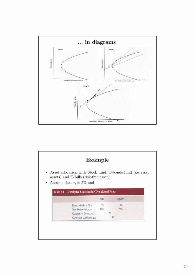
Example

• Asset allocation with Stock fund, T-bonds fund (i.e. risky assets) and T-bills (risk-free asset)

• Assume that rf = 5% and

15

Example (cont’d)

Example (cont’d)

• In order to find a solution of our Step 2 we have to maximize the slope of the CAL (under the constraint that the sum of the weights = 1)

• In the case of two risky assets

• For more than 2 risky assets (normal case) we need to rely on MS Excel (or other computer programs)

( )max

. . 1

p fpw

p

ii

E r rS

s t w

σ−

=

=∑

( ) ( ) ( )( ) ( ) ( ) ( ) ( )

21 2 2 1 2

1 2 21 2 2 1 1 2 1 2

2 1

cov ,

cov ,

1

f f

f f f f

E r r E r r r rw

E r r E r r E r r E r r r r

w w

σ

σ σ

⎡ ⎤ ⎡ ⎤− − −⎣ ⎦ ⎣ ⎦=⎡ ⎤ ⎡ ⎤ ⎡ ⎤− + − − − + −⎣ ⎦ ⎣ ⎦ ⎣ ⎦

= −

16

Example (cont’d)

• The solution of Step 2 is called tangency portfolio and comprises only risky assets. In our case the tangency portfolio comprises the two risky funds with weights

[ ] [ ][ ] [ ] [ ]

( ) ( ) ( )

( ) ( )

1

2

tan

2 2tan

tan

8 5 400 13 5 720.40

8 5 400 13 5 144 8 5 13 5 721 0.40 0.60

0.4 8 0.6 13 11%

0.4 144 0.6 400 2 0.4 0.6 72 14.2%

11 5 0.4214.2

w

wE r

S

σ

− − −= =

− + − − − + −

= − =

= × + × =

= × + × + × × × =

−= =

Example (cont’d)

17

Example (cont’d)

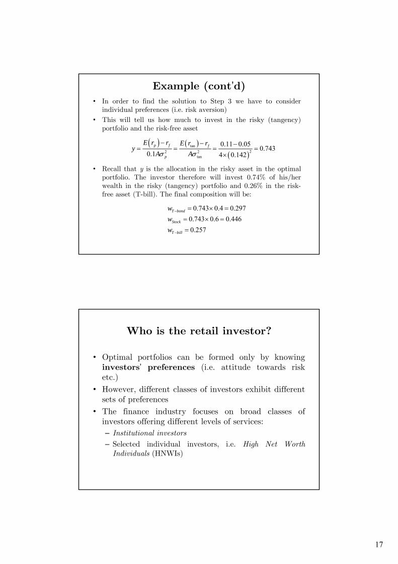
• In order to find the solution to Step 3 we have to consider individual preferences (i.e. risk aversion)

• This will tell us how much to invest in the risky (tangency) portfolio and the risk-free asset

• Recall that y is the allocation in the risky asset in the optimal portfolio. The investor therefore will invest 0.74% of his/her wealth in the risky (tangency) portfolio and 0.26% in the risk-free asset (T-bill). The final composition will be:

( ) ( )( )

tan22 2

tan

0.11 0.05 0.7430.1 4 0.142

p f f

p

E r r E r ry

A Aσ σ− − −

= = = =×

0.743 0.4 0.2970.743 0.6 0.4460.257

T bond

Stock

T bill

www

−

−

= × == × =

=

Who is the retail investor?

• Optimal portfolios can be formed only by knowing investors’ preferences (i.e. attitude towards risk etc.)

• However, different classes of investors exhibit different sets of preferences

• The finance industry focuses on broad classes of investors offering different levels of services:

– Institutional investors

– Selected individual investors, i.e. High Net Worth Individuals (HNWIs)

18

HNWIs

• HNWIs are individuals who hold more than USD 1 million in financial-asset wealth. The high end of this class is termed Ultra-HNWIs (i.e. individuals with more than USD 30 million in financial asset)

HNWIs in 2005

• In 2005 globally HNWIs are 8.7 million with different geographical area concentrations. The geographical concentration of Ultra-HNWIs is similar to HNWIs but with a stronger dominance of North American individuals.

• Economic growth and robust stock market growth are the main factors driving the population growth of HNWIs in 2005. South Korea, India, Russia and South Africa experienced the highest growth in HNWI population.

19

HNWIs in 2005 (cont’d)

HNWIs in 2005 (cont’d)

20

HNWIs in 2005 (cont’d)

HNWIs in 2005 (cont’d)

21

HNWIs in 2005 (cont’d)

Where Does the Wealth Come From?

22

HNWIs vs Institutional Investors

HNWIs vs Institutional Investors (cont’d)

• HNWIs:

– Use disciplined investment methodologies (no sentiments or hearding)

– Frequently rebalance their portfolios (dynamic vsstatic)

– Base investment selection upon fundamental analysis

– Balance risk, reward and liquidity of overall investments

23

HNWIs Expectations

Readings

• Bodie, Kane and Marcus

– Chapters 6, 7 (7.5 excluded)

• Other readings (optional)

– Merrill Lynch, Capgemini, World Wealth Report1997-2006. Downloadable at

www.us.capgemini.com/worldwealthreport06