Embed Size (px)
Citation preview
Pore-Scale Modelling of Three-Phase Flow
Mohammad Piri
Centre for Petroleum Studies
Department of Earth Science and Engineering
Imperial College London
London SW7 2AZ, UK
A thesis submitted in fulfillment of the requirements for
the degree of Doctor of Philosophy of the University of London
and the Diploma of Imperial College
December, 2003
Abstract
We present a three-dimensional network model to simulate two- and three-phase
capillary dominated processes at the pore level. The displacement mechanisms in-
corporated in the model are based on the physics of multi-phase flow observed in
micromodel experiments. All the important features of immiscible fluid flow at the
pore-scale, such as wetting layers, spreading layers of the intermediate-wet phase,
hysteresis and wettability alteration are implemented in the model. Wettability al-
teration allows any values for the advancing and receding oil/water, gas/water and
gas/oil contact angles to be assigned. Multiple phases can be present in each pore
or throat (element), in wetting and spreading layers, as well as occupying the cen-
tre of the pore space. In all, some thirty different generic fluid configurations for
two- and three-phase flow are analyzed. Double displacement and layer reformation
are implemented as well as direct two-phase displacement and layer collapse events.
Every element has a circular, square or triangular cross-section. A random network
that represents the pore space in Berea sandstone is used in this study. The model
computes relative permeabilities, saturation paths, and capillary pressures for any
displacement sequence. A methodology to track a given three-phase saturation path
is presented that enables us to compare predicted and measured relative permeabil-
ities on a point-by-point basis. A new and robust displacement based clustering
algorithm is presented. We predict measured relative permeabilities for two-phase
flow in a water-wet system. We then successfully predict the steady-state oil, water
and gas three-phase relative permeabilities measured by Oak [1]. We also study sec-
ondary and tertiary gas injection into media of different wettability and initial oil
saturation and interpret the results in terms of pore-scale displacement processes.
3
4
The list of publications as a result of this research is as follows:
• M.J. Blunt, M.D. Jackson, M. Piri, and P.H. Valvatne. Detailed physics,
predictive capabilities and macroscopic consequences for pore-network models
of multiphase flow. Advances in Water Resources, 25(8-12):1069-1089, 2002.
• M. Piri, and M.J. Blunt. Pore-scale modeling of three-phase flow in mixed-
wet systems. Paper SPE 77726, Proceedings of the SPE Annual Technical Con-
ference and Exhibition, San Antonio, Texas, 29 September-2 October, 2002.
• P.H. Valvatne, M. Piri, X. Lopez, and M.J. Blunt. Predictive pore-scale
modeling of single and multiphase flow. Transport in Porous Media (in press)
• M. Piri, and M.J. Blunt. Three-dimensional mixed-wet random pore-scale
network model of two- and three-phase flow in porous media. Physical Review
E (submitted).

Acknowledgments
Firstly and most importantly, I would like to express my deepest gratitude to the
Almighty and the All-knowing Allah, who, if you believe in him, will never dash
your hopes.
Martin holds a place very close to my heart. I am extremely fortunate to have
him as my very close friend and supervisor. I have enormously benefited from his
invaluable scientific and spiritual support, advice, and continuous encouragement
throughout my work with him. Martin, I am deeply affected by your integrity and
commitment. Thank you so much.
Imperial College London, in particular the Department of Earth Science and
Engineering - Center for Petroleum Studies - is very special to me. This is because
of the excellent people that I have had the honor of working with. I would like to
take this opportunity to thank them, especially the faculty, students and staff for
their support, guidance and friendship. It means a lot to me.
I feel fortunate to have made so many good friends during my time here. I wish
to thank them all, too many to name, but here are a few: Eguono-Oghene Obi,
Per H. Valvatne, Hiroshi Okabe, Mohammed Al-Gharbi, Pascal Audigane, Maryam
Khorram, Alimirza Gholipour, Robert Leckenby, Reza Banki, Branko Bijeljic, Azzan
Al-Yaarubi, Rifaat A. M. Al-Mjeni, Ali Dehghani, Arash Soleimani, Ginevra Di
Donato, Hooman Sadrpanah, Thomas von Schroeter, Djamel Ouzzane, and Xavier
Lopez.
My gratitude extends to Prof. Ken S. Sorbie from Heriot-Watt University, and
Prof. Peter R. King from Imperial College London, for serving on my examination
committee.
A special mention with my sincere gratefulness goes to Prof. P̊al-Eric Øren from
Statoil for his continuous and invaluable comments throughout my work on Pore-
Scale Modelling. I also feel indebted to the following people for their comments,
stimulating discussions and encouragements: Prof. Dave Waldren, Dr. Carlos A.
Grattoni , Dr. M.I.J. van Dijke, Dr. Matthew D. Jackson, Prof. Tadeusz W. Patzek,
5
6
Prof. Abbas Firoozabadi, and Prof. Muhammad Sahimi.
I would like to acknowledge the sponsors of Imperial College Consortium on
Pore-Scale Modelling, i.e. BHP, EPSRC, Gaz de France, JNOC, PDVSA-Intevep,
Schlumberger, Shell, Statoil, and the UK Department of Trade and Industry, for
their generous and continued support of my research.
I also wish to try and express my gratitude to Dr. Mike Ala, Prof. Alain C.
Gringarten and Dr. Hamid Hatamian for their kind help and attention before and
after I started at Imperial College.
Last, but by no means least, is my family. I would like to thank them for their
love, kindness, encouragement, and understanding. Mom, Dad, Lamia, Amoo Reza,
Fatemeh, Masoomeh, Ali, Elaheh, Cobra, and Morteza, with love I dedicate this
thesis, that I have worked very hard for, to you.
Contents
Abstract 3
Acknowledgments 5
Contents 9
List of Figures 13
List of Tables 15
1 Introduction 16
2 Physics of Three-Phase Flow at the Pore-Level 21
2.1 Spreading Coefficients and Interfacial Tensions . . . . . . . . . . . . . 21
2.2 Three-Phase Contact Angles . . . . . . . . . . . . . . . . . . . . . . . 23
2.3 Wettability Alteration and Contact Angle Hysteresis . . . . . . . . . 24
2.4 Spreading and Wetting Layers . . . . . . . . . . . . . . . . . . . . . . 26
3 Literature Review 27
3.1 Previously Developed Three-Phase Pore-Scale Network Models . . . . 27
4 Displacement Mechanisms 36
4.1 Porous Medium . . . . . . . . . . . . . . . . . . . . . . . . . . . . . . 36
4.2 Pore and Throat Cross-Sectional Shapes . . . . . . . . . . . . . . . . 37
4.3 Pressure Difference Across an Interface . . . . . . . . . . . . . . . . . 41
4.4 Displacement Mechanisms . . . . . . . . . . . . . . . . . . . . . . . . 42
4.4.1 Drainage . . . . . . . . . . . . . . . . . . . . . . . . . . . . . . 42
4.4.2 Imbibition . . . . . . . . . . . . . . . . . . . . . . . . . . . . . 48
4.5 Layer Collapse and Formation . . . . . . . . . . . . . . . . . . . . . . 60
4.5.1 Identical Fluids on Two Sides of a Layer . . . . . . . . . . . . 60
7
8
4.5.2 Different Fluids on Two Sides of a Layer . . . . . . . . . . . . 61
5 Two- and Three-Phase Fluid Generic Configurations 66
5.1 Definitions . . . . . . . . . . . . . . . . . . . . . . . . . . . . . . . . . 70
5.2 Configuration Changes . . . . . . . . . . . . . . . . . . . . . . . . . . 71
5.2.1 Configuration Group A . . . . . . . . . . . . . . . . . . . . . . 74
5.2.2 Configuration Group B . . . . . . . . . . . . . . . . . . . . . . 76
5.2.3 Configuration Group C . . . . . . . . . . . . . . . . . . . . . . 77
5.2.4 Configuration Group D . . . . . . . . . . . . . . . . . . . . . . 79
5.2.5 Configuration Group E . . . . . . . . . . . . . . . . . . . . . . 80
5.2.6 Configuration Group F . . . . . . . . . . . . . . . . . . . . . . 81
5.2.7 Configuration Group G . . . . . . . . . . . . . . . . . . . . . . 83
5.2.8 Configuration Group H . . . . . . . . . . . . . . . . . . . . . 85
5.2.9 Configuration Group I . . . . . . . . . . . . . . . . . . . . . . 86
5.2.10 Configuration Group J . . . . . . . . . . . . . . . . . . . . . . 86
5.2.11 Configuration Group K . . . . . . . . . . . . . . . . . . . . . 88
6 Pore-Scale Network Modelling 89
6.1 Continuity and Clustering . . . . . . . . . . . . . . . . . . . . . . . . 89
6.1.1 Hoshen & Kopelman Algorithm . . . . . . . . . . . . . . . . . 89
6.1.2 Displacement Based Algorithm . . . . . . . . . . . . . . . . . 90
6.2 How to Choose the Right Displacement . . . . . . . . . . . . . . . . . 95
6.3 How to Treat the Trapped Clusters, Associated Radii of Curvatures
and Displacements . . . . . . . . . . . . . . . . . . . . . . . . . . . . 99
6.3.1 Coalescence . . . . . . . . . . . . . . . . . . . . . . . . . . . . 101
6.3.2 When a Trapped Cluster Breaks into Smaller Ones . . . . . . 103
6.4 Multiple Displacements . . . . . . . . . . . . . . . . . . . . . . . . . . 103
6.5 Saturation Computation . . . . . . . . . . . . . . . . . . . . . . . . . 110
6.5.1 Area Open to Flow . . . . . . . . . . . . . . . . . . . . . . . . 110
6.6 Conductances - Absolute and Relative Permeabilities . . . . . . . . . 112
6.7 Saturation Path Tracking . . . . . . . . . . . . . . . . . . . . . . . . 117
7 Two- and Three-Phase Relative Permeabilities 119
7.1 Comparison with Experiment . . . . . . . . . . . . . . . . . . . . . . 119
7.1.1 Two-Phase Simulations/Primary Drainage . . . . . . . . . . . 120
7.1.2 Two-Phase Simulations/Imbibition . . . . . . . . . . . . . . . 120
7.1.3 Three-Phase Simulations . . . . . . . . . . . . . . . . . . . . . 122
9
7.2 Simulation of Different Processes . . . . . . . . . . . . . . . . . . . . 130
7.2.1 Secondary Gas Injection . . . . . . . . . . . . . . . . . . . . . 131
7.2.2 Comparison of Secondary and Tertiary Gas Injection . . . . . 134
7.2.3 Tertiary Gas Injection into Water Flood Residual Oil . . . . . 136
7.2.4 Effects of Wettability . . . . . . . . . . . . . . . . . . . . . . . 143
8 Final Remarks 148
8.1 Conclusions . . . . . . . . . . . . . . . . . . . . . . . . . . . . . . . . 148
8.2 Recommendations for Future Work . . . . . . . . . . . . . . . . . . . 150
Bibliography 151
Appendix 181
A Threshold Layer Collapse Capillary Pressure 181
B Parameters in the Model 186
List of Figures
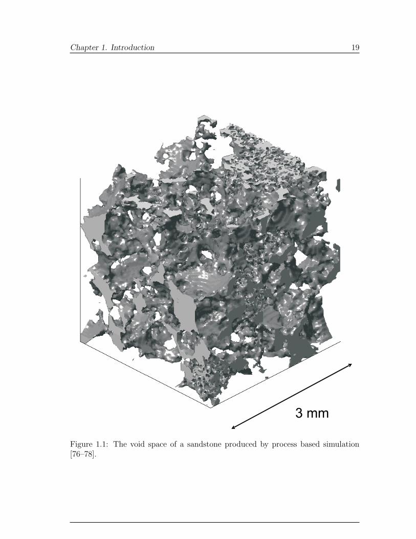
1.1 The void space of a sandstone produced by process based simulation. 19
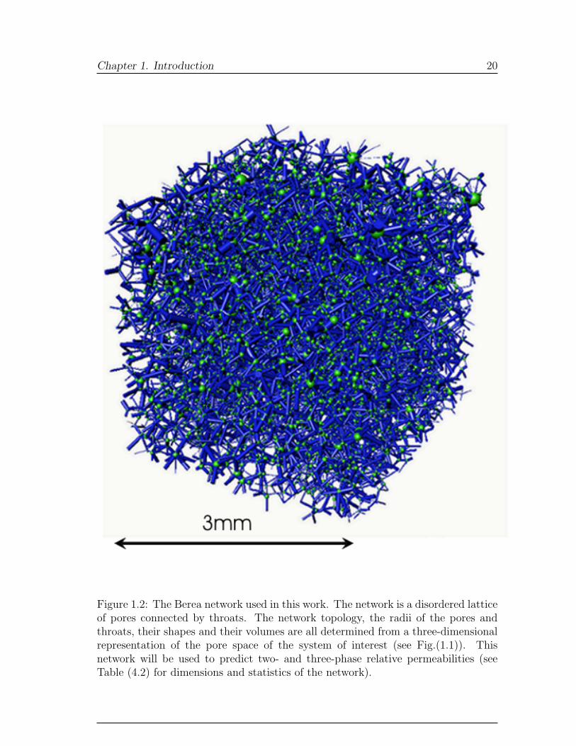
1.2 The Berea network used in this work. . . . . . . . . . . . . . . . . . . 20
2.1 Different three-phase systems. . . . . . . . . . . . . . . . . . . . . . . 22
2.2 Horizontal force balance in three two-phase systems. . . . . . . . . . . 23
4.1 Elements with different cross-sectional shape. . . . . . . . . . . . . . 37
4.2 Pore and throat size distributions for the Berea network. . . . . . . . 39
4.3 An element with irregular triangular cross-section. . . . . . . . . . . 41
4.4 Distribution of shape factor vs. the second largest corner half angle
in irregular triangles. . . . . . . . . . . . . . . . . . . . . . . . . . . . 42
4.5 Different types of interface. . . . . . . . . . . . . . . . . . . . . . . . . 43
4.6 Spherical meniscus in a capillary. . . . . . . . . . . . . . . . . . . . . 43
4.7 Effective perimeter and area for elements with cylindrical and angular
cross-section. . . . . . . . . . . . . . . . . . . . . . . . . . . . . . . . 45
4.8 Imbibition by invasion of an MTM - conditions of the AM’s at the
corners. . . . . . . . . . . . . . . . . . . . . . . . . . . . . . . . . . . 52
4.9 Diffrent pore-body filling events for imbibition in a pore. . . . . . . . 59
4.10 A layer sandwiched between identical fluids residing in the corner and
centre. . . . . . . . . . . . . . . . . . . . . . . . . . . . . . . . . . . . 61
4.11 A layer sandwiched between different fluids residing in the corner and
centre (θhI < θh
II). . . . . . . . . . . . . . . . . . . . . . . . . . . . . . 62
4.12 A layer sandwiched between different fluids residing in the corner and
centre (θ1 > θ2). . . . . . . . . . . . . . . . . . . . . . . . . . . . . . . 64
4.13 A layer sandwiched between different fluids (negative interfaces and
double layers). . . . . . . . . . . . . . . . . . . . . . . . . . . . . . . . 65
5.1 One- and Two-phase configurations. . . . . . . . . . . . . . . . . . . . 68
5.2 Three-phase configurations. . . . . . . . . . . . . . . . . . . . . . . . 69
10
11
5.3 Possible configuration changes to configurations A and B. . . . . . . 75
5.4 Possible configuration changes to configurations C and D. . . . . . . 78
5.5 Possible configuration changes to configurations E and F . . . . . . . 82
5.6 Possible configuration changes to configurations G and H. . . . . . . 84
5.7 Possible configuration changes to configurations I, J , and K. . . . . . 87
6.1 Flow chart used to determine clusters of each phase. . . . . . . . . . . 91
6.2 Double Drainage in Water-wet Systems. . . . . . . . . . . . . . . . . 105
6.3 Double Imbibition in Water-wet Systems. . . . . . . . . . . . . . . . . 106
6.4 Imbibition-Drainage in Water-wet Systems. . . . . . . . . . . . . . . . 106
6.5 Corners with a sandwiched layer. . . . . . . . . . . . . . . . . . . . . 111
6.6 Schematic assemblies of pores connected to each other by throats. . . 114
6.7 Schematic presentation of saturation tracking method. . . . . . . . . 118
7.1 Comparison of experimental and predicted relative permeabilities dur-
ing primary drainage in Berea sandstone. . . . . . . . . . . . . . . . . 120
7.2 Comparison of measured and predicted two-phase oil/water relative
permeabilities for imbibition in Berea sandstone. . . . . . . . . . . . . 121
7.3 Comparison of measured and predicted two-phase gas/oil relative per-
meabilities for imbibition in Berea sandstone. . . . . . . . . . . . . . 122
7.4 Comparison of measured and predicted two-phase gas/water relative
permeabilities for imbibition in Berea sandstone. . . . . . . . . . . . . 123
7.5 Comparison of measured and predicted three-phase oil relative per-
meability during gas injection. . . . . . . . . . . . . . . . . . . . . . . 123
7.6 Comparison of measured and predicted three-phase gas relative per-
meability during gas injection. . . . . . . . . . . . . . . . . . . . . . . 124
7.7 Comparison of measured and predicted three-phase water relative
permeability during gas injection. . . . . . . . . . . . . . . . . . . . . 125
7.8 Comparison of measured and tracked saturation paths for Experiment
9 - Sample 13 of Oak experiments [1]. . . . . . . . . . . . . . . . . . . 126
7.9 Comparison of measured and predicted three-phase oil relative per-
meabilities for Experiment 9 - Sample 13 of Oak experiments [1]. . . . 127
7.10 Comparison of measured and predicted three-phase gas relative per-
meabilities for Experiment 9 - Sample 13 of Oak experiments [1]. . . . 127
7.11 Comparison of measured and predicted three-phase water relative
permeabilities for Experiment 9 - Sample 13 of Oak experiments [1]. . 128
12
7.12 Comparison of measured and tracked saturation paths for Experiment
10 - Sample 14 of Oak experiments [1]. . . . . . . . . . . . . . . . . . 128
7.13 Comparison of measured and predicted three-phase oil relative per-
meabilities for Experiment 10 - Sample 14 of Oak experiments [1]. . . 129
7.14 Comparison of measured and predicted three-phase gas relative per-
meabilities for Experiment 10 - Sample 14 of Oak experiments [1]. . . 130
7.15 Saturation paths for secondary gas injection with different initial oil
saturations in a spreading system. . . . . . . . . . . . . . . . . . . . . 131
7.16 Three-phase oil relative permeabilities for secondary gas injection
with different initial oil saturations. . . . . . . . . . . . . . . . . . . . 132
7.17 Three-phase gas relative permeabilities for secondary gas injection
with different initial oil saturations. . . . . . . . . . . . . . . . . . . 133
7.18 Three-phase water relative permeabilities for secondary gas injection
with different initial oil saturations. . . . . . . . . . . . . . . . . . . 133
7.19 Comparison of three-phase oil relative permeability for secondary and
tertiary gas injection with an initial oil saturation of 0.55. . . . . . . 134
7.20 Comparison of three-phase gas relative permeability for secondary
and tertiary gas injection with an initial oil saturation of 0.55. . . . . 135
7.21 Comparison of three-phase water relative permeability for secondary
and tertiary water injection with an initial oil saturation of 0.55. . . . 136
7.22 Three-phase oil relative permeability for tertiary gas injection into
water flood residual oil (Soi = 0.384) and for secondary gas injection
with a similar initial oil saturation (Soi = 0.38). . . . . . . . . . . . . 137
7.23 Pore and throat occupancy as a function of size after primary drainage
to So = 0.38. . . . . . . . . . . . . . . . . . . . . . . . . . . . . . . . . 138
7.24 Pore and throat occupancy as a function of size after water flooding. 138
7.25 Pore and throat occupancy as a function of size during tertiary gas
injection into water flood residual oil when So ≈ 0.23. . . . . . . . . 139
7.26 Pore and throat occupancy as a function of size during tertiary gas
injection into water flood residual oil when So ≈ 0.16. . . . . . . . . 140
7.27 Pore and throat occupancy as a function of size during tertiary gas
injection into water flood residual oil when So ≈ 0.07. . . . . . . . . 141
7.28 Pore and throat occupancy as a function of size during tertiary gas
injection into water flood residual oil when So ≈ 0.01. . . . . . . . . 141
13
7.29 Three-phase gas relative permeability for tertiary gas injection into
water flood residual oil (Soi = 0.384) and for secondary gas injection
with a similar initial oil saturation (Soi = 0.38). . . . . . . . . . . . . 142
7.30 Three-phase water relative permeability for tertiary gas injection into
water flood residual oil (Soi = 0.384) and for secondary gas injection
with a similar initial oil saturation (Soi = 0.38). . . . . . . . . . . . . 142
7.31 Trapped oil saturation as a function of gas saturation during tertiary
gas injection into water flood residual oil. . . . . . . . . . . . . . . . . 143
7.32 Oil and water relative permeabilities of water flooding in: (I) water-
wet, θaow = 30◦ − 70◦ (system A), and (II) oil-wet, θa
ow = 110◦ − 180◦
(system B) Berea sandstone. . . . . . . . . . . . . . . . . . . . . . . . 144
7.33 Pore and throat occupancy as a function of size after water flooding
in the oil-wet system. . . . . . . . . . . . . . . . . . . . . . . . . . . . 145
7.34 Effects of wettability on three-phase oil relative permeability. . . . . . 146
7.35 Effects of wettability on three-phase water relative permeability. . . . 146
7.36 Effects of wettability on three-phase water relative permeability. . . . 147
A.1 A layer sandwiched between identical fluids residing in the corner and
centre. . . . . . . . . . . . . . . . . . . . . . . . . . . . . . . . . . . . 181
List of Tables
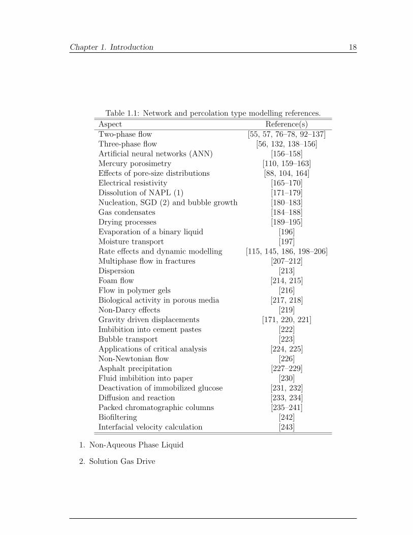
1.1 Network and percolation type modelling references. . . . . . . . . . . 18
4.1 Network parameters read by the model. . . . . . . . . . . . . . . . . 38
4.2 Berea network statistics. . . . . . . . . . . . . . . . . . . . . . . . . . 40
4.3 Threshold capillary pressures for piston-like and pore-body filling dis-
placements with layers of the invading phase contributing to the dis-
placement - oil to water, gas to water and gas to oil. . . . . . . . . . . 49
4.4 Threshold capillary pressures for piston-like and pore-body filling dis-
placements with layers of the invading phase contributing to the dis-
placement - water to oil, water to gas, and oil to gas. . . . . . . . . . 50
4.5 Threshold capillary pressures for piston-like and pore-body filling dis-
placements with no layers of the invading phase contributing to the
displacement - oil to water, gas to water and gas to oil. . . . . . . . . 51
4.6 Threshold capillary pressures for piston-like and pore-body filling dis-
placements with no layers of the invading phase contributing to the
displacement - water to oil, water to gas, and oil to gas. . . . . . . . . 51
4.7 Threshold capillary pressures for snap-off displacements - oil to water,
gas to water and gas to oil. . . . . . . . . . . . . . . . . . . . . . . . . 57
4.8 Threshold capillary pressures for snap-off displacements - water to
oil, water to gas, and oil to gas. . . . . . . . . . . . . . . . . . . . . . 58
5.1 The range of contact angles for different configurations. . . . . . . . . 67
6.1 Criteria for connectivity of phase locations. . . . . . . . . . . . . . . . 92
6.2 Multiple displacements search categories (continuous-trapped; c-t). . . 97
6.3 Multiple displacements search categories (trapped-continuous; t-c). . . 98
6.4 Multiple displacements search categories (trapped-trapped; t-t). . . . 98
6.5 Possible double displacements in strongly water-wet systems. . . . . . 104
6.6 Possible double displacements in strongly oil-wet systems. . . . . . . . 104
14
15
6.7 Possible double displacements in weakly oil-wet systems. . . . . . . . 105
7.1 Interfacial tensions and spreading coefficient (mN/m) used in this work.120
7.2 Contact angles (degrees) used predict the experiments. . . . . . . . . 122
7.3 Contact angles (degrees) used to simulate different processes. . . . . . 131
7.4 The number of different types of displacement for tertiary gas injec-
tion into water flood residual oil (Soi = 0.384) and for secondary gas
injection with a similar initial oil saturation (Soi = 0.38). . . . . . . . 140
Chapter 1
Introduction
The simultaneous flow of three phases - oil, water and gas - in porous media is of great
interest in many areas of science and technology, such as petroleum reservoir and
environmental engineering. Three fluid flow occurs in enhanced oil recovery schemes
including tertiary gas injection into oil and water, gas cap expansion, solution gas
drive, gravity drainage, water flooding with different initial oil and gas saturations,
steam injection, thermal flooding, depressurization below the bubble point, and
water alternate gas (WAG) injection. In an environmental context three-phase flow
occurs when a non-aqueous phase liquid (NAPL), leaking from an underground
storage tank for instance, migrates through the unsaturated zone and may coexists
with water and air (gaseous phase).
In order to understand fluid flow in porous media, one needs to know the consti-
tutive relationships between macroscopic properties of the system such as relative
permeabilities, capillary pressures, and fluid saturations. These relationships are
used in macroscopic partial differential equations to describe the transport of fluid.
The determination of constitutive relationships is complicated as they are dependent
on the fluids’ properties, the pore space, and the saturation history.
Experimental measurements of three-phase relative permeabilities and capillary
pressures have been the subject of several studies [1–30], but they are extremely
difficult to perform and at low saturation the results are very uncertain [16, 23,
31, 32]. Two independent fluid saturations are required to define a three-phase
system and there is an infinite number of possible fluid arrangements making a
comprehensive suite of experimental measurements for all three-phase displacements
impossible. This is why numerical simulations of three-phase flow almost always
rely on available empirical correlations to predict relative permeability and capillary
pressure from measured two-phase properties [4, 20, 22, 33–54]. These models may
16
Chapter 1. Introduction 17
give predictions that vary as much as an order of magnitude from each other, or
from direct measurements, since they have little or no physical basis [43, 53, 55].
It is important to have a reliable physically-based tool that can provide plausible
estimates of macroscopic properties. Any theoretical or numerical approach to this
problem not only needs a detailed understanding of the multiphase displacement
mechanisms at the pore level but also an accurate and realistic characterization of
the structure of the porous medium [56]. During the last two decades our knowl-
edge of the physics of two- and three-phase flow at the pore level has considerably
increased through experimental investigation of displacements in core samples and
micromodels [57–72]. To describe the geometry of the pore space several authors
have developed different statistical [73–75] and process based [76–78] techniques. In
addition the pore space can be imaged directly using micro CT tomography [79, 80].
An example of a three-dimensional pore space image of a sandstone is shown in Fig.
(1.1). It is possible to simulate multi-phase flow directly on a three-dimensional
pore-space image by solving Navier Stokes equations or by using Lattice-Boltzman
techniques [81–84]. However, for capillary controlled flow with multiple phases, these
methods become cumbersome and computationally expensive.
An attractive alternative approach is to describe the pore space as a network
of pores connected by throats with some idealized geometry (see Fig.(1.2)) [78,
85]. Then a series of displacement steps in each pore or throat are combined to
simulate multiphase flow. Fatt [86–88] initiated this approach by using a regular
two-dimensional network to find capillary pressure and relative permeability. Since
then, the capabilities of network models have improved enormously and have been
applied to describe many different processes. Table 1.1 lists some of the recent
applications of network modelling. Recent advances in pore-scale modelling have
been reviewed by Celia et al. [89], Blunt [90], and Blunt et al. [91].
For a random close packing of spheres Bryant and co-workers were able to predict
permeability, elastic and electrical properties and relative permeability [107, 111,
244]. Øren et al. extended this approach by reconstructing a variety of sandstones
and generating topologically equivalent networks from them. Using these networks
several authors have been able to predict relative permeability and oil recovery for
a variety of systems [76–78, 118, 127, 132, 136].
In this work we extend this predictive approach to three-phase flow. Before
reviewing previous three-phase network models in detail, we review the fundamentals
of contact angles, spreading coefficient and wettability alteration as well as spreading
and wetting layers.
Chapter 1. Introduction 18
Table 1.1: Network and percolation type modelling references.
Aspect Reference(s)Two-phase flow [55, 57, 76–78, 92–137]Three-phase flow [56, 132, 138–156]Artificial neural networks (ANN) [156–158]Mercury porosimetry [110, 159–163]Effects of pore-size distributions [88, 104, 164]Electrical resistivity [165–170]Dissolution of NAPL (1) [171–179]Nucleation, SGD (2) and bubble growth [180–183]Gas condensates [184–188]Drying processes [189–195]Evaporation of a binary liquid [196]Moisture transport [197]Rate effects and dynamic modelling [115, 145, 186, 198–206]Multiphase flow in fractures [207–212]Dispersion [213]Foam flow [214, 215]Flow in polymer gels [216]Biological activity in porous media [217, 218]Non-Darcy effects [219]Gravity driven displacements [171, 220, 221]Imbibition into cement pastes [222]Bubble transport [223]Applications of critical analysis [224, 225]Non-Newtonian flow [226]Asphalt precipitation [227–229]Fluid imbibition into paper [230]Deactivation of immobilized glucose [231, 232]Diffusion and reaction [233, 234]Packed chromatographic columns [235–241]Biofiltering [242]Interfacial velocity calculation [243]
1. Non-Aqueous Phase Liquid
2. Solution Gas Drive
Chapter 1. Introduction 19
3 mm
Figure 1.1: The void space of a sandstone produced by process based simulation[76–78].
Chapter 1. Introduction 20
Figure 1.2: The Berea network used in this work. The network is a disordered latticeof pores connected by throats. The network topology, the radii of the pores andthroats, their shapes and their volumes are all determined from a three-dimensionalrepresentation of the pore space of the system of interest (see Fig.(1.1)). Thisnetwork will be used to predict two- and three-phase relative permeabilities (seeTable (4.2) for dimensions and statistics of the network).
Chapter 2
Physics of Three-Phase Flow at
the Pore-Level
2.1 Spreading Coefficients and Interfacial Tensions
The ability of oil to spread on water in the presence of gas is described by the
spreading coefficient which is a representation of the force balance where the three
phases meet. If the interfacial tensions are found by contacting pairs of pure fluids
in the absence of the third, the coefficient is called initial and is defined by [245]:
Cis = σgw − σgo − σow (2.1)
where σ is an interfacial tension between two phases labeled o, w, and g to stand
for oil, water, and gas respectively. However, when three phases are present si-
multaneously, the interfacial tensions are different from those in two-phase systems.
For instance, the gas/water interfacial tension may be significantly lower than its
two-phase value because oil may cover the interface by a thin film of molecular
thickness [246]. The other two-phase interfacial tensions may also vary when the
third phase is present. If the three phases remain long enough in contact, thermo-
dynamic equilibrium will be reached when liquids become mutually saturated. In
these circumstances the spreading coefficient is named equilibrium and is given by
Eq. (2.2), which is either negative or zero [245].
Ceqs = σeq
gw − σeqgo − σeq
ow (2.2)
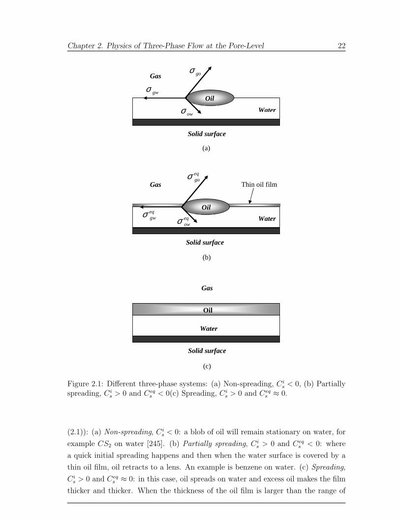
Three-phase systems may be divided into one of the following cases (see Fig.
21
Chapter 2. Physics of Three-Phase Flow at the Pore-Level 22
Solid surface
Water
Gas
Oil
Solid surface
Water
Gas
Oil gwσ
goσ
owσ
Solid surface
Water
Gas
Oil eqgwσ
eqgoσ
eqowσ
Thin oil film
(a)
(b)
(c)
Figure 2.1: Different three-phase systems: (a) Non-spreading, Cis < 0, (b) Partially
spreading, Cis > 0 and Ceq
s < 0(c) Spreading, Cis > 0 and Ceq
s ≈ 0.
(2.1)): (a) Non-spreading, Cis < 0: a blob of oil will remain stationary on water, for
example CS2 on water [245]. (b) Partially spreading, Cis > 0 and Ceq
s < 0: where
a quick initial spreading happens and then when the water surface is covered by a
thin oil film, oil retracts to a lens. An example is benzene on water. (c) Spreading,
Cis > 0 and Ceq
s ≈ 0: in this case, oil spreads on water and excess oil makes the film
thicker and thicker. When the thickness of the oil film is larger than the range of

Chapter 2. Physics of Three-Phase Flow at the Pore-Level 23
intermolecular forces the equilibrium spreading coefficient becomes zero. Soltrol, a
mixture of hydrocarbons, is an example of this case [71].
In the rest of the work, we will drop the superscript eq and always assume that
we are dealing with interfacial tensions at equilibrium.
2.2 Three-Phase Contact Angles
The contact angle is defined as the angle between the two-phase line and the solid
surface measured through the denser phase. In a three phase system a horizontal
force balance can be written for each of the three pairs of fluids, i.e. oil-water, gas-
water, and gas-oil, residing on a solid to obtain Young’s equation (see Fig. (2.2)):
owσ
owθ wsσ osσ
Solid
Oil Water
gwσ
gwθ wsσ gsσ
Solid
Gas Water
goσ
goθ osσ gsσ
Solid
Gas Oil
(a) (b)
(c)
Figure 2.2: Horizontal force balance in three two-phase systems: (a) oil/water/solid,(b) gas/water/solid, and (c) gas/oil/solid.
σos = σws + σow cos θow (2.3)
σgs = σws + σgw cos θgw (2.4)
σgs = σos + σgo cos θgo (2.5)
Chapter 2. Physics of Three-Phase Flow at the Pore-Level 24
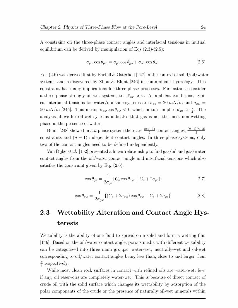
A constraint on the three-phase contact angles and interfacial tensions in mutual
equilibrium can be derived by manipulation of Eqs.(2.3)-(2.5):
σgw cos θgw = σgo cos θgo + σow cos θow (2.6)
Eq. (2.6) was derived first by Bartell & Osterhoff [247] in the context of solid/oil/water
systems and rediscovered by Zhou & Blunt [246] in contaminant hydrology. This
constraint has many implications for three-phase processes. For instance consider
a three-phase strongly oil-wet system, i.e. θow ≈ π. At ambient conditions, typi-
cal interfacial tensions for water/n-alkane systems are σgo = 20 mN/m and σow =
50 mN/m [245]. This means σgw cos θgw < 0 which in turn implies θgw > π2. The
analysis above for oil-wet systems indicates that gas is not the most non-wetting
phase in the presence of water.
Blunt [248] showed in a n phase system there are n(n−1)2
contact angles, (n−1)(n−2)2
constraints and (n − 1) independent contact angles. In three-phase systems, only
two of the contact angles need to be defined independently.
Van Dijke et al. [152] presented a linear relationship to find gas/oil and gas/water
contact angles from the oil/water contact angle and interfacial tensions which also
satisfies the constraint given by Eq. (2.6):
cos θgo =1
2σgo
{Cs cos θow + Cs + 2σgo} (2.7)
cos θgw =1
2σgw
{(Cs + 2σow) cos θow + Cs + 2σgo} (2.8)
2.3 Wettability Alteration and Contact Angle Hys-
teresis
Wettability is the ability of one fluid to spread on a solid and form a wetting film
[146]. Based on the oil/water contact angle, porous media with different wettability
can be categorized into three main groups: water-wet, neutrally-wet and oil-wet
corresponding to oil/water contact angles being less than, close to and larger thanπ2
respectively.
While most clean rock surfaces in contact with refined oils are water-wet, few,
if any, oil reservoirs are completely water-wet. This is because of direct contact of
crude oil with the solid surface which changes its wettability by adsorption of the
polar components of the crude or the presence of naturally oil-wet minerals within
Chapter 2. Physics of Three-Phase Flow at the Pore-Level 25
the rock. This makes any values of oil/water and consequently gas/water and gas/oil
contact angles possible [249–253]. Kovscek et al. [251] developed a model where the
wettability of the rock surface is assumed to be altered by the direct contact of
oil. Before a porous medium is invaded by oil it is assumed to be full of water and
water-wet. Once it is invaded by oil, a thin film of water prevents oil touching the
solid surface directly. But at a threshold capillary pressure, this film can collapse
and allows oil to contact the solid surface and change its wettability. Regions of the
pore space not contacted by oil remain water-wet.
The contact angle also depends on the direction of displacement. This difference
between advancing, i.e. wetting phase displacing the non-wetting one, and receding,
i.e. non-wetting phase displacing the wetting one, contact angles may be as large
as 50◦ - 90◦ [245, 254, 255] depending on surface roughness, surface heterogeneity,
swelling, rearrangement or alteration of the surface by solvent [245].
To accommodate any type of displacement process, we assign eight contact angles
to each pore and throat: θPDow (oil displacing water in an element that has not changed
its wettability before), θPDgw (gas displacing water in an element that has not changed
its wettability before), and six contact angles when the wettability has been altered:
θaow (water displacing oil), θr
ow (oil displacing water), θagw (water displacing gas), θr
gw
(gas displacing water), θago (oil displacing gas), θr
go (gas displacing oil).
There is an ambiguity in defining a third contact angle from Eq. (2.6) if advanc-
ing and receding values are different. For instance, imagine water is being injected
into oil and gas where the appropriate gas/water and oil/water contact angles to
be used are θagw and θa
ow respectively. Now if one uses Eq. (2.6) to find the third
contact angle, θgo, it is not clear that the calculated value is the advancing or re-
ceding gas/oil contact angle. This problem is also evident when one uses Eqs. (2.7)
and (2.8), where it is not known, for example, which oil/water contact angle, i.e.
advancing or receding, should be used to calculate receding gas/oil contact angle
needed, for example, in gas injection into oil and water.
In this work, we first decide on the values of two of the contact angles and then
calculate the third one using Eq. (2.6). We use θrow and θr
go to calculate a θgw. We
also use θaow and θa
go to find another value of θgw. The smaller of two values of θgw is
considered as receding and the larger one as the advancing value. We always make
sure in every single pore and throat, the receding contact angle for each phase is
less than or equal to the advancing value, i.e. θrij ≤ θa
ij.
Chapter 2. Physics of Three-Phase Flow at the Pore-Level 26
2.4 Spreading and Wetting Layers
During primary drainage, oil can occupy centres of the pore space, leaving water as
a wetting layer in the corners and crevices of the pore space. During subsequent
cycles of water and/or gas injection these water layers are still present and maintain
continuity of water.
After gas injection into an element containing oil in the centre and water in
wetting layers, gas will occupy the centre and it is possible that oil will remain in a
layer sandwiched between the gas and water. These are called spreading layers; as
we discuss later their stability is related to the spreading coefficient, contact angles,
corner angles and capillary pressures, and are likely to be present in spreading
systems.
Later, we will present detailed analysis of possible pore space configurations in
terms of displacement history, contact angles and spreading coefficient. However, to
motivate the critique of previous pore-scale models of three-phase flow, we need to
emphasize the definition of some key terms.
A spreading system has Cs = 0 and oil spontaneously forms layers between water
and gas in the pore space. A non-spreading system has Cs < 0 and while oil layers
can also be present [72, 256, 257] they tend to be stable for more restricted range
of capillary pressures. Also, we refer to wetting and spreading layers - these layers
are typically a few microns in thickness and have a non-negligible hydraulic conduc-
tivity and maintain phase continuity. In contrast, films are of molecular thickness
(of order a nanometer) and have negligible conductivity and do not contribute to
phase continuity - where present films simply modify the apparent, or equilibrium,
interfacial tensions, as discussed above.
Chapter 3
Literature Review
3.1 Previously Developed Three-Phase Pore-Scale
Network Models
Here we present a detailed review of previously developed three-phase network mod-
els.
Heiba et al. [138] extended statistical network modelling previously used for
two-phase systems [96, 108] to three-phase flow. A Bethe lattice, or Cayley network
was used to represent the porous medium. Relative permeabilities were calculated
from Stinchcombe’s formula [258] using new series approximations from percolation
theory. Only a single phase could occupy a throat. A given fluid was considered to
be able to flow only when the site that it occupied was a member of a continuous
flow path from the inlet to the outlet. The displacement of one phase by another
was controlled by accessibility and local entry capillary pressure. Six groups of dis-
placement were considered: gas into oil, oil into gas, gas into water, water into gas,
water into oil, and oil into water. Two spreading systems were investigated where
in the first one gas and water were displacing oil while in the second case water
and oil were displacing oil and gas. The results showed that the gas and water
relative permeabilities were functions of only their own saturations. Oil layers pre-
vented the direct contact of gas and water. Oil isoperms were found to be strongly
curved, meaning that the oil relative permeability was not only a function of its own
saturation. Extensions of the theory to handle the complications involved by the
effects of wettability and phase swelling due to mass transfer were also discussed. It
was concluded that three-phase relative permeabilities are generally path functions
rather than state functions (function of saturation only) except in particular situa-
27
Chapter 3. Literature Review 28
tions such as when two phases are separated by the third. This model used rather
simple networks and displacement rules.
Soll & Celia [139] developed a computational model of capillary-dominated two-
and three-phase movement at the pore level to simulate capillary pressure-saturation
relationships in a water-wet system. Regular two- or three-dimensional networks
of pores, connected to each other by throats, were used to represent the porous
medium. Hysteresis was modelled by using advancing and receding values for the
contact angles for each pair of fluids. Every pore was able to accommodate one fluid
at a time as well as wetting layers. Viscous forces were considered to be negligible
but the effects of gravity were included to modify the local capillary pressures. In
order to reproduce their micromodel experiments [66], oil as a spreading phase was
allowed to advance ahead of a continuous invasion front. Several pores could be filled
simultaneously. This model was the first to incorporate layer flow in three-phase
network modelling albeit in a rather ad hoc fashion. The results were compared
with capillary pressure-saturation results and fluid distributions from the two- and
three-fluid micromodel experiments. The amount of oil layer flow was used as a
fitting parameter. Predicted two-phase air/water and oil/water capillary pressures
were in good agreement with measured values [66] although the model did not so
successfully match three-phase data. The model was not used to calculate relative
permeabilities.
Øren et al. [140] described details of the pore level displacement mechanisms
taking place during immiscible gas injection into waterflood residual oil (tertiary gas
injection) which then were incorporated into a two-dimensional strongly water-wet
square network model with rectangular links and spherical pores in order to compute
oil recovery in spreading and non-spreading systems. Simulated recoveries compared
very well with the measured values from micromodel experiments [63, 64]. The
authors described a double drainage mechanism where gas displaces trapped oil that
displaces water allowing immobile oil to become connected boosting oil recovery. Oil
recovery decreased with decreasing spreading coefficient. In non-spreading systems,
the probability of direct gas-water displacement was high and capillary fingering of
gas resulted in early gas breakthrough and low oil recovery. In spreading systems,
oil reconnection was more effective and direct gas/oil displacement was preferred. It
was concluded that a simple invasion percolation algorithm [94, 259] including the
spreading layers works well in mimicking the complex three-phase behaviour seen in
micromodels. In this work, relative permeabilities were not calculated.
Pereira et al. [56, 147] developed a dynamic two-dimensional network model for
Chapter 3. Literature Review 29
drainage-dominated three-phase flow in strongly water- and oil-wet systems when
both capillary and viscous forces were important. The displacement mechanisms in
spreading and non-spreading systems were described by generalization of two-phase
displacement mechanisms. Both pores and throats were assumed to be lenticular
in cross-section allowing wetting and spreading layers to be present. No volumes
were allocated to the throats and layers and there was no pressure drop in the
pores. Resistance to the flow through the throats was modelled using the mean
hydraulic radius concept, i.e. twice the ratio of area open to flow to wetted perimeter.
Pressure of a fluid in a throat was an interpolation of pressures of the same fluid
in the neighbouring pores. Trapping of different fluids was considered only for
non-spreading systems. Coalescence and reconnection of trapped clusters was also
simulated. Pores could be occupied by two or three bulk fluids at the same time
separated by flat interface(s). The simulated recoveries at gas breakthrough were
compared against measured values in micromodels [64]. As in Øren et al. [140],
a large difference between the recoveries in spreading and non-spreading systems
was reported for water-wet cases due to existence of oil layers in the spreading
systems. The highest recovery, 85%, was found for the oil-wet case. This was
because continuous wetting layers prevented trapping of oil. The oil recovery was
much lower, 14%, for the water-wet case in a non-spreading system. This was
because there were no spreading layers of oil. Even when layers were present for
the spreading system, the oil recovery was much lower, 40%, in a water-wet medium
than for the oil-wet case. Water in water-wet systems played the same role as oil in
oil-wet systems – water recoveries in water-wet spreading and non-spreading systems
were high. It was confirmed that the high oil recoveries were due to the presence
of wetting or spreading oil layers, despite the fact that the conductance of a layer
of water or oil in a throat was only around 1% of the conductance of a throat
full of a single phase. In non-spreading systems, direct water displacement by gas
was preferred over gas-oil-water double displacement leading to low oil recovery. An
order of magnitude reduction in the simulated conductivity of the oil layers decreased
oil recovery and made the behaviour of the spreading system similar to that of a non-
spreading system. Also a reduction in initial oil saturation for tertiary gas injection
decreased the oil recovery. This was true for both spreading and non-spreading
systems indicating that the recovery of the intermediate wetting phase is strong
function of saturation history. This was reported to be consistent with experiments
by Dria et al. [23] and Oak [1, 21]. It was also concluded that the recovery of the
wetting fluid is independent of the saturation history. Relative permeabilities were
Chapter 3. Literature Review 30
not calculated in this work.
Paterson et al. [141] developed a water-wet percolation model to study the
effects of spatial correlations in the pore size distributions on three-phase relative
permeabilities and residual saturations. This was an extension of their previous
work on two-phase systems [117]. Fractal maps derived from fractional Brownian
and Levy motion (fBm and fLm) were used to assign pore size. A simple site
percolation model with trapping was used. Trapping was incorporated based on
Hoshen-Kopelman algorithm [260]. In three-phase simulations direct displacement of
oil and water by gas and also double drainage were implemented. The model assigned
the same volume to all pores and so the fraction of sites occupied by a phase gave
its saturation. All the sites were assumed to have the same conductivity regardless
of their radii. The simulation results for correlated properties showed lower residual
saturations in comparison to uncorrelated ones. Incorporating a bedding orientation
to the spacial-correlations had a major impact on relative permeability. When the
bedding was parallel to the flow direction, the relative permeabilities were greater
and residual saturations lower than those when bedding was perpendicular to the
flow. This was also the case for two-phase relative permeabilities [117]. The effects
of spreading coefficient were also studied. Similar to previous authors [56, 140, 147]
it was shown that the less negative the spreading coefficient, the lower the final
residual oil saturation. For more negative spreading coefficients direct gas to oil and
gas to water displacements are preferred over double drainage. This effect was more
significant for correlated systems.
Fenwick & Blunt [142, 143] developed a three-phase network model for strongly
water-wet systems. A regular cubic network composed of pores and throats with
equilateral triangular or square cross-sections was used. Oil/water and gas/water
contact angles were considered to be zero. Two and three-phase displacement mecha-
nisms including oil layer flow observed in micromodel experiments were incorporated
in the model. Double drainage was generalized to allow any of six types of double
displacement where one phase displaces a second that displaces a third as observed
by Keller et al. [72]. The model was able to simulate any sequence of oil, water and
gas injection. Using a geometrical analysis, a criterion for stability of oil layers was
derived which was dependent on oil/water and gas/oil capillary pressures, contact
angles, equilibrium interfacial tensions, and the corner half angle. It was argued that
oil layers could be present even for negative spreading coefficient systems. Using a
simple calculation [246] it was shown that the layers are of order a micron across
or thicker in the corners, roughness and grooves of the pore space. The work was
Chapter 3. Literature Review 31
the first to estimate conductance of an oil layer which then was used to compute
oil relative permeability. It was shown that at low oil saturation the oil relative
permeability should vary quadratically with saturation, as observed experimentally
[13, 261–263].
It was shown that in three-phase systems relative permeabilities and oil recover-
ies are strong functions of saturation path. An iterative methodology which coupled
a physically-based network model with a 1-D three-phase Buckley-Leverett simula-
tor was developed in order to find the correct saturation path for a given process
with known initial condition and injection fluid [143]. This enabled the network
model to compute the properties for the right displacement sequence. The three-
phase relative permeabilities were called self-consistent when the saturation path
that was used by the network model to compute them will be exactly produced
by the conventional three-phase Buckley-Leverett simulator if the network model
relative permeabilities were used in the flow equations to compute the macroscopic
flow. Self-consistent relative permeabilities for secondary and tertiary gas injection
into different initial oil saturations were presented. The resultant saturation paths
compared well qualitatively with experimental data by Grader & O’Meara [13]. The
paths in the oil/water vs. gas/oil capillary pressure space were all located in the
region where oil layers were stable meaning that oil did not get trapped. Oil rel-
ative permeabilities for different initial conditions were different from each other,
consistent with several experimental studies [1, 2, 16, 25, 43].
Mani & Mohanty [144, 145] also used a regular cubic network of pores and throats
to simulate three-phase flow in water-wet systems. Pores and throats were consid-
ered to be spherical and cylindrical respectively. The oil/water capillary pressure
was fixed at its original value during the gas invasion processes. The parameters
of the network were tuned to match two-phase mercury-air experimental capillary
pressures for Berea sandstone [92].
Both dynamic and quasi-static simulations were carried out. The work had
two important features: (I) Dynamic simulation of capillary-controlled gas invasion,
where it was assumed each phase pressure was not constant across the network.
(II) Re-injection of the produced fluids at the outlet of the medium into the inlet
in order to simulate larger systems. This was used to see whether trapped oil
ganglia become reconnected by double drainage to form spanning clusters. The
two-phase processes were simulated at low capillary number using traditional quasi-
static assumptions. Pressure drops across pores were ignored. The model included
fluid flow through wetting and spreading layers. A fixed conductance was assigned to

Chapter 3. Literature Review 32
oil layers. For the capillary pressure histories used, no stable oil layers were observed
in both spreading and non-spreading systems. Gas invasion was modelled by three
displacement mechanisms: direct gas/water, direct gas/oil, and double drainage.
For each displacement a potential was considered which was the difference between
the pressures of two involved fluids minus the threshold capillary pressure of the
displacement. The displacement with the largest potential was carried out first.
Re-injection of fluids was simulated by replacing the fluid distribution in the inlet
zone by the fluids in the outlet zone. The process was terminated after steady
state was reached at the imposed pressure conditions, i.e. when no further gas
invasion was possible at the imposed capillary pressure. The final oil saturation in
spreading systems was zero. The capillary pressure curves obtained from dynamic
and quasi-static simulations were virtually identical. For non-spreading systems
with a low oil/water capillary pressure, drainage of water and oil occurred with
similar probability. Displacement of water from the medium created trapped oil
clusters that were surrounded by gas. Due to the assumed absence of oil layers
in non-spreading systems, oil ganglia could not be displaced by gas at any gas/oil
capillary pressure. The water relative permeability was a function of the water
saturation alone for both two-phase and three-phase systems, and was not dependent
on the saturation history, spreading coefficient and the imposed oil/water capillary
pressure. Similarly, for spreading three-phase systems, it was shown that gas relative
permeability is a function of its own saturation only and do not depend on the
imposed oil/water capillary pressure. But for non-spreading systems, the three-
phase gas relative permeability was different from the two-phase drainage curves
and were dependent on the oil/water capillary pressure, spreading coefficient and
the saturation history. The three-phase oil relative permeability was a function of
the oil saturation, the imposed oil/water capillary pressure, the spreading coefficient
and the saturation history in both spreading and non-spreading systems. The effect
of spreading coefficient and saturation history on three-phase relative permeability
was consistent with other network modelling studies [56, 140, 142, 143, 147] and
experimental measurements [1, 2, 16, 25, 43].
Laroche et al. [125, 146] developed a pore network model to predict the effects
of wettability heterogeneities with different patterns and spatial distributions on
displacement mechanisms, sweep efficiency, and fluid distribution in gas injection
into oil and water. A dalmatian type of wettability heterogeneity was used with
continuous water-wet surfaces enclosing discontinuous regions of oil-wet surfaces or
vice-versa. A series of three-phase glass micro-model experiments with different
Chapter 3. Literature Review 33
wettabilities were also carried out. Measured oil/water contact angles for the water-
wet and oil-wet surfaces were 0◦ and 105◦ respectively. n-Dodecane, water, and
nitrogen were the three fluids used in the experiments. All the two-phase interfacial
tensions, densities, and viscosities were measured. The initial spreading coefficient
was 7.3mN/m and hence the oil was assumed to be spreading. The capillary number
throughout the experiments was approximately 10−5 indicating capillary controlled
displacement. A 2-D regular pore and throat network was used to simulate the
experiments. All the throats had triangular cross-sections while the pores were
circular cylinders. The pore and throat size distributions were similar to those
of Berea sandstone. Saturations, conductances, and relative permeabilities were
calculated using similar techniques to Fenwick & Blunt [142]. The fluid distributions
at the end of two- and three-phase simulations were in good qualitative agreement
with those found experimentally.
Hui & Blunt [264, 265] developed a mixed-wet model of three-phase flow for a
bundle of capillary tubes. The tubes had different sizes and were equilateral triangle
in cross-section. Wettability alteration was modelled by changing the wettability of
surfaces that came into contact with oil after primary drainage. This enabled the
model to simulate three-phase flow with any combination of oil/water, gas/water,
and gas/oil contact angles. In all some ten fluid configuration were considered. Pri-
mary drainage, water flooding, and tertiary gas injection were simulated. The effects
of wettability, spreading coefficient and initial oil saturation on relative permeabil-
ities were investigated. Possible configuration changes during each process along
with the threshold capillary pressure of each change were presented. The stability
of layers in different configurations and capillary pressures at which they collapse
was discussed. We will extend this approach to study 30 different possible fluid
configurations in three-phase flow and will incorporate them in a three-dimensional
random network model.
Lerdahl et al. [149] used the technique developed by Bakke et al. [76] to recon-
struct a three-dimensional void space, Fig. (1.1), and then convert it to a pore and
throat network, Fig. (1.2), for use in a water-wet network model to study drainage-
dominated three-phase flow. Simulated results were compared successfully against
the experimental data by Oak [1]. We will use a similar network in our studies and
also compare our predictions against Oak’s experiments [1]. In our study we will
compare results on a point-by-point basis using our saturation tracking algorithm
and extend the model to mixed-wet systems following the approach of Hui & Blunt
[264, 265].
Chapter 3. Literature Review 34
Larsen et al. [150] used a water-wet three-dimensional cubic pore network model
based on the work of Fenwick & Blunt [142, 143] to simulate a series of micromodel
experiments of WAG (water alternate gas) injection processes. All the pores and
throats were assumed to have square cross-sections. The network model was used
in an iterative procedure similar to the one used by Fenwick & Blunt [143] to find
self-consistent saturation paths. Three WAG injections with different gas/water
injection ratios were carried out.
Van Dijke et al. [151–153] presented a process-based mixed-wet model of three-
phase flow using a bundle of capillary tubes with circular cross-sections to study
the saturation dependencies of capillary pressures and relative permeabilities for
spreading and non-spreading systems. Larger pores were considered to be oil-wet
and the smaller ones water-wet. It was shown that based on interfacial tensions
and contact angles the three-phase saturation space could be divided up to three
different regions with a different intermediate-wet phase. The relative permeability
of this phase was a function of two saturations. Also the capillary pressure between
the most wetting and non-wetting phases is dependent on two saturations. The
relative permeabilities of the other two phases were a function of only their own
saturation in this region. The authors extended this approach to determine the
functional dependency of relative permeability and capillary pressure for media of
arbitrary wettability.
Van Dijke et al. [154, 155] developed a regular three-dimensional three-phase
network model for systems with different wettability expanding on thier previous
studies on bundles of capillary tubes. Every element was allowed to have a different
oil/water contact angle and Eqs. (2.7) and (2.8) were used to determine the gas/oil
and gas/water contact angles [152]. While layers were not incorporated explicitly in
saturation or conductance computations, they were allowed to establish continuity
of different phases. The model was a cubic array of only throats with a circular
cross-section. The coordination number could be changed by removing throats from
the network. An extensive series of simulations of three-phase flow was performed.
For networks with a high coordination number, the saturation dependencies were
qualitatively similar to those predicted for capillary bundles. As the coordination
number was reduced, connectivity was impaired and trapping became significant.
The authors also compared their network simulations with micromodel experiments
of WAG [266, 267] where there were repeated cycles of water and gas flooding.
To reproduce the results, they incorporated multiple displacements where a train
trapped clusters may displace each other until there is invasion into a connected
Chapter 3. Literature Review 35
phase. They suggested that such multiple displacements were significant in WAG
flooding. While certainly such displacements were observed in the micromodel ex-
periments, we suggest that in three-dimensional displacements the phases are likely
to be better connected and so the movement of trapped ganglia is less significant.
We will only consider double displacements in this work.
The conclusion of this section is that while many three-phase pore-scale dis-
placement mechanisms are well understood, and the generic functionality of relative
permeability has been discussed, three-phase network models to date have not ad-
dressed the full range of possible configurations in mixed-wet systems and their
predictive powers are limited.
The network model described here combines three essential components: (1) a
description of the pore space and its connectivity that mimics real systems; (2) a
physically-based model of wettability alteration; and (3) a full description of fluid
configurations for two- and three-phase flow. This will enable us to predict three-
phase relative permeabilities for media of arbitrary wettability using geologically
realistic networks.
Comparison of the experimental and predicted relative permeabilities in three-
phase systems is only possible if both have identical saturation paths. This is because
macroscopic properties in three-phase systems are strongly dependent on saturation
history of the system. In this work, we present an algorithm to simulate experimen-
tal saturation paths and predict relative permeabilities to compare with measured
values.
Chapter 4
Displacement Mechanisms
4.1 Porous Medium
In recent years, several advances have been made in the construction of realistic
representations of porous media. Øren, Bakke and co-workers [76–78] have devel-
oped random network models based on the pore space geometry of the rock of
interest. The model is derived either from a direct three-dimensional image of the
pore space obtained from micro CT scanning, or from simulating the geological
processes by which the rock was formed, see Fig.(1.1). Many other authors have
also developed techniques to derive pore structures from a variety of measurements
[75, 80, 107, 111, 130, 163, 244, 268–278]. While such approaches are not routine,
and the correct pore-space characterization of carbonates is very much an open ques-
tion, for simple sandstones there are reliable methods for determining an equivalent
network structure that attempts to mimic the properties of the real pore space.
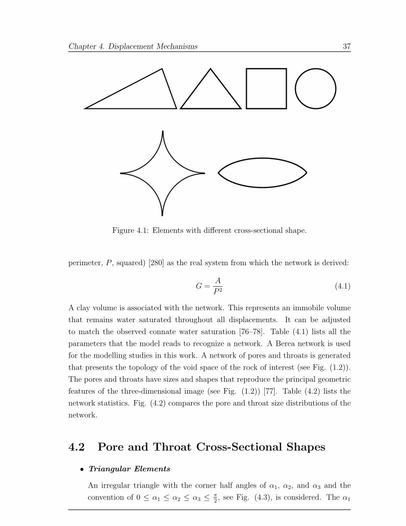
In cross-section, individual pores and throats are often modelled as triangles and
high-order polygons [279, 280]. This allows wetting phase to occupy the corners when
the non-wetting phase fills the centre. As well as triangular cross-section elements,
authors have used geometries with circular [154, 155], square [142, 143, 150], star-
shape [112, 166, 168–170], and lenticular [56, 147] cross-sections (see Fig.(4.1)) to
represent pores and throats.
The network model in this work reads as input any two or three-dimensional
regular or random network comprised of pores connected by throats. Each pore or
throat is assigned a total volume, an inscribed radius and a shape. The inscribed
radius is used to assign a capillary entry pressure during multiphase flow. In this
model the pore and throats have a scalene triangular, square or circular cross-section.
The cross-section has the same shape factor G (ratio of cross-sectional area, A, to
36
Chapter 4. Displacement Mechanisms 37
Figure 4.1: Elements with different cross-sectional shape.
perimeter, P , squared) [280] as the real system from which the network is derived:
G =A
P 2(4.1)
A clay volume is associated with the network. This represents an immobile volume
that remains water saturated throughout all displacements. It can be adjusted
to match the observed connate water saturation [76–78]. Table (4.1) lists all the
parameters that the model reads to recognize a network. A Berea network is used
for the modelling studies in this work. A network of pores and throats is generated
that presents the topology of the void space of the rock of interest (see Fig. (1.2)).
The pores and throats have sizes and shapes that reproduce the principal geometric
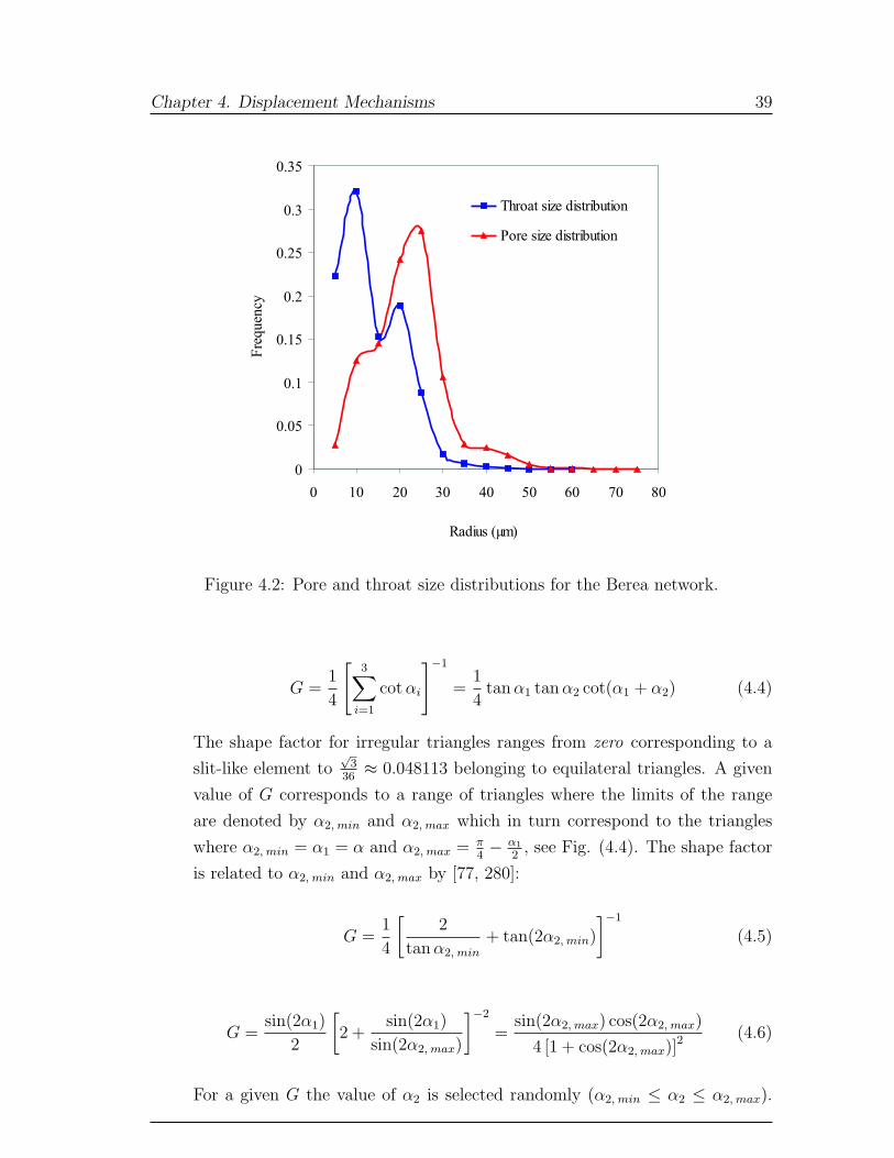
features of the three-dimensional image (see Fig. (1.2)) [77]. Table (4.2) lists the
network statistics. Fig. (4.2) compares the pore and throat size distributions of the
network.
4.2 Pore and Throat Cross-Sectional Shapes
• Triangular Elements
An irregular triangle with the corner half angles of α1, α2, and α3 and the
convention of 0 ≤ α1 ≤ α2 ≤ α3 ≤ π2, see Fig. (4.3), is considered. The α1
Chapter 4. Displacement Mechanisms 38
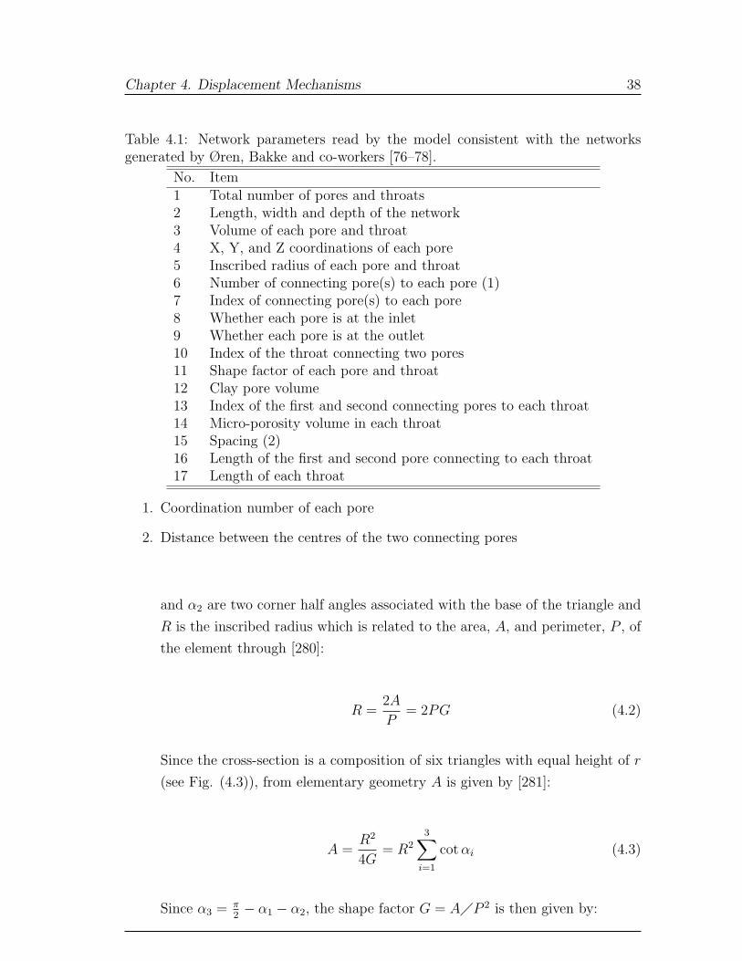
Table 4.1: Network parameters read by the model consistent with the networksgenerated by Øren, Bakke and co-workers [76–78].
No. Item1 Total number of pores and throats2 Length, width and depth of the network3 Volume of each pore and throat4 X, Y, and Z coordinations of each pore5 Inscribed radius of each pore and throat6 Number of connecting pore(s) to each pore (1)7 Index of connecting pore(s) to each pore8 Whether each pore is at the inlet9 Whether each pore is at the outlet10 Index of the throat connecting two pores11 Shape factor of each pore and throat12 Clay pore volume13 Index of the first and second connecting pores to each throat14 Micro-porosity volume in each throat15 Spacing (2)16 Length of the first and second pore connecting to each throat17 Length of each throat
1. Coordination number of each pore
2. Distance between the centres of the two connecting pores
and α2 are two corner half angles associated with the base of the triangle and
R is the inscribed radius which is related to the area, A, and perimeter, P , of
the element through [280]:
R =2A
P= 2PG (4.2)
Since the cross-section is a composition of six triangles with equal height of r
(see Fig. (4.3)), from elementary geometry A is given by [281]:
A =R2
4G= R2
3∑i=1
cot αi (4.3)
Since α3 = π2− α1 − α2, the shape factor G = A�P 2 is then given by:
Chapter 4. Displacement Mechanisms 39
0
0.05
0.1
0.15
0.2
0.25
0.3
0.35
0 10 20 30 40 50 60 70 80
Fre
quen
cy
Throat size distribution
Pore size distribution
Radius (µm)
Figure 4.2: Pore and throat size distributions for the Berea network.
G =1
4
[3∑
i=1
cot αi
]−1
=1
4tan α1 tan α2 cot(α1 + α2) (4.4)
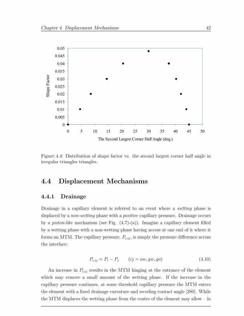
The shape factor for irregular triangles ranges from zero corresponding to a
slit-like element to√
336≈ 0.048113 belonging to equilateral triangles. A given
value of G corresponds to a range of triangles where the limits of the range
are denoted by α2, min and α2, max which in turn correspond to the triangles
where α2, min = α1 = α and α2, max = π4− α1
2, see Fig. (4.4). The shape factor
is related to α2, min and α2, max by [77, 280]:
G =1
4
[2
tan α2, min
+ tan(2α2, min)
]−1
(4.5)
G =sin(2α1)
2
[2 +
sin(2α1)
sin(2α2, max)
]−2
=sin(2α2, max) cos(2α2, max)
4 [1 + cos(2α2, max)]2 (4.6)
For a given G the value of α2 is selected randomly (α2, min ≤ α2 ≤ α2, max).
Chapter 4. Displacement Mechanisms 40
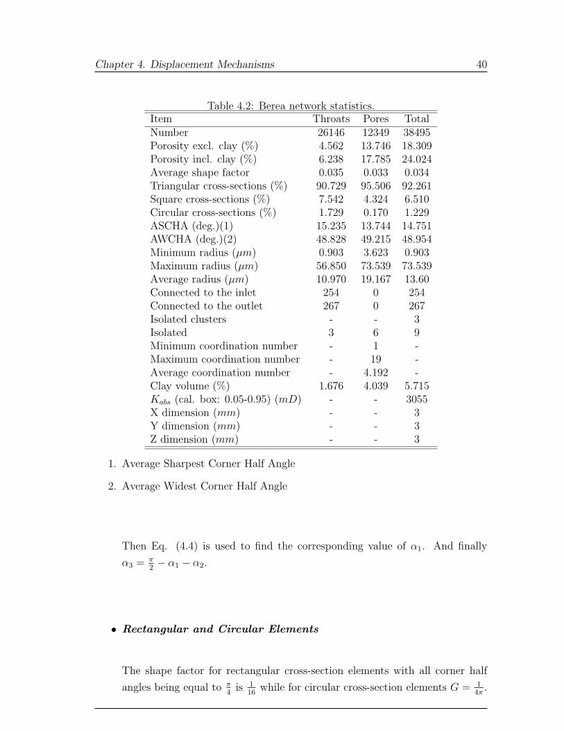
Table 4.2: Berea network statistics.Item Throats Pores TotalNumber 26146 12349 38495Porosity excl. clay (%) 4.562 13.746 18.309Porosity incl. clay (%) 6.238 17.785 24.024Average shape factor 0.035 0.033 0.034Triangular cross-sections (%) 90.729 95.506 92.261Square cross-sections (%) 7.542 4.324 6.510Circular cross-sections (%) 1.729 0.170 1.229ASCHA (deg.)(1) 15.235 13.744 14.751AWCHA (deg.)(2) 48.828 49.215 48.954Minimum radius (µm) 0.903 3.623 0.903Maximum radius (µm) 56.850 73.539 73.539Average radius (µm) 10.970 19.167 13.60Connected to the inlet 254 0 254Connected to the outlet 267 0 267Isolated clusters - - 3Isolated 3 6 9Minimum coordination number - 1 -Maximum coordination number - 19 -Average coordination number - 4.192 -Clay volume (%) 1.676 4.039 5.715Kabs (cal. box: 0.05-0.95) (mD) - - 3055X dimension (mm) - - 3Y dimension (mm) - - 3Z dimension (mm) - - 3
1. Average Sharpest Corner Half Angle
2. Average Widest Corner Half Angle
Then Eq. (4.4) is used to find the corresponding value of α1. And finally
α3 = π2− α1 − α2.
• Rectangular and Circular Elements
The shape factor for rectangular cross-section elements with all corner half
angles being equal to π4
is 116
while for circular cross-section elements G = 14π
.
Chapter 4. Displacement Mechanisms 41
R
1α 2α
3α
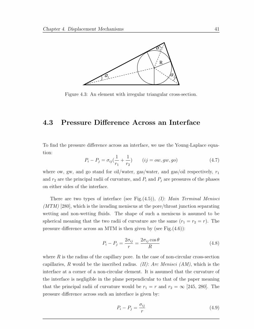
Figure 4.3: An element with irregular triangular cross-section.
4.3 Pressure Difference Across an Interface
To find the pressure difference across an interface, we use the Young-Laplace equa-
tion:
Pi − Pj = σij(1
r1
+1
r2
) (ij = ow, gw, go) (4.7)
where ow, gw, and go stand for oil/water, gas/water, and gas/oil respectively, r1
and r2 are the principal radii of curvature, and Pi and Pj are pressures of the phases
on either sides of the interface.
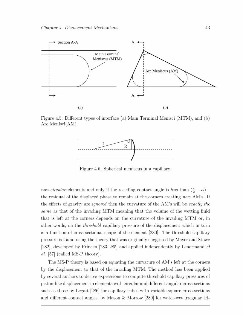
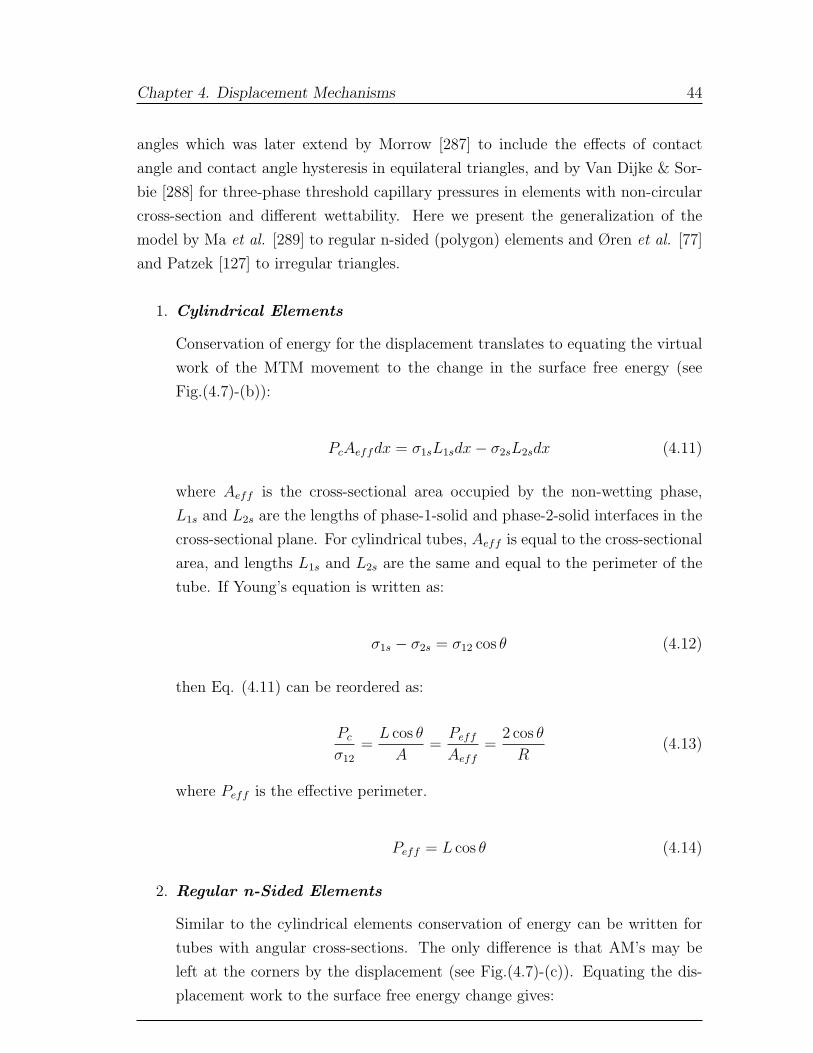
There are two types of interface (see Fig.(4.5)), (I): Main Terminal Menisci
(MTM) [280], which is the invading meniscus at the pore/throat junction separating
wetting and non-wetting fluids. The shape of such a meniscus is assumed to be
spherical meaning that the two radii of curvature are the same (r1 = r2 = r). The
pressure difference across an MTM is then given by (see Fig.(4.6)):
Pi − Pj =2σij
r=
2σij cos θ
R(4.8)
where R is the radius of the capillary pore. In the case of non-circular cross-section
capillaries, R would be the inscribed radius. (II): Arc Menisci (AM), which is the
interface at a corner of a non-circular element. It is assumed that the curvature of
the interface is negligible in the plane perpendicular to that of the paper meaning
that the principal radii of curvature would be r1 = r and r2 = ∞ [245, 280]. The
pressure difference across such an interface is given by:
Pi − Pj =σij
r(4.9)
Chapter 4. Displacement Mechanisms 42
0
0.005
0.01
0.015
0.02
0.025
0.03
0.035
0.04
0.045
0.05
0 5 10 15 20 25 30 35 40 45 50
The Second Largest Corner Half Angle (deg.)
Shap
eF
acto
r
Figure 4.4: Distribution of shape factor vs. the second largest corner half angle inirregular triangles triangles.
4.4 Displacement Mechanisms
4.4.1 Drainage
Drainage in a capillary element is referred to an event where a wetting phase is
displaced by a non-wetting phase with a positive capillary pressure. Drainage occurs
by a piston-like mechanism (see Fig. (4.7)-(a)). Imagine a capillary element filled
by a wetting phase with a non-wetting phase having access at one end of it where it
forms an MTM. The capillary pressure, Pc,ij, is simply the pressure difference across
the interface:
Pc,ij = Pi − Pj (ij = ow, gw, go) (4.10)
An increase in Pc,ij results in the MTM hinging at the entrance of the element
which may remove a small amount of the wetting phase. If the increase in the
capillary pressure continues, at some threshold capillary pressure the MTM enters
the element with a fixed drainage curvature and receding contact angle [280]. While
the MTM displaces the wetting phase from the centre of the element may allow – in
Chapter 4. Displacement Mechanisms 43
(a) (b)
Section A-A
Main Terminal Meniscus (MTM)
A
A
Arc Meniscus (AM)
Figure 4.5: Different types of interface (a) Main Terminal Menisci (MTM), and (b)Arc Menisci(AM).
qr
R
Figure 4.6: Spherical meniscus in a capillary.
non-circular elements and only if the receding contact angle is less than (π2− α) –
the residual of the displaced phase to remain at the corners creating new AM’s. If
the effects of gravity are ignored then the curvature of the AM’s will be exactly the
same as that of the invading MTM meaning that the volume of the wetting fluid
that is left at the corners depends on the curvature of the invading MTM or, in
other words, on the threshold capillary pressure of the displacement which in turn
is a function of cross-sectional shape of the element [280]. The threshold capillary
pressure is found using the theory that was originally suggested by Mayer and Stowe
[282], developed by Princen [283–285] and applied independently by Lenormand et
al. [57] (called MS-P theory).
The MS-P theory is based on equating the curvature of AM’s left at the corners
by the displacement to that of the invading MTM. The method has been applied
by several authors to derive expressions to compute threshold capillary pressures of
piston-like displacement in elements with circular and different angular cross-sections
such as those by Legait [286] for capillary tubes with variable square cross-sections
and different contact angles, by Mason & Morrow [280] for water-wet irregular tri-
Chapter 4. Displacement Mechanisms 44
angles which was later extend by Morrow [287] to include the effects of contact
angle and contact angle hysteresis in equilateral triangles, and by Van Dijke & Sor-
bie [288] for three-phase threshold capillary pressures in elements with non-circular
cross-section and different wettability. Here we present the generalization of the
model by Ma et al. [289] to regular n-sided (polygon) elements and Øren et al. [77]
and Patzek [127] to irregular triangles.
1. Cylindrical Elements
Conservation of energy for the displacement translates to equating the virtual
work of the MTM movement to the change in the surface free energy (see
Fig.(4.7)-(b)):
PcAeffdx = σ1sL1sdx− σ2sL2sdx (4.11)
where Aeff is the cross-sectional area occupied by the non-wetting phase,
L1s and L2s are the lengths of phase-1-solid and phase-2-solid interfaces in the
cross-sectional plane. For cylindrical tubes, Aeff is equal to the cross-sectional
area, and lengths L1s and L2s are the same and equal to the perimeter of the
tube. If Young’s equation is written as:
σ1s − σ2s = σ12 cos θ (4.12)
then Eq. (4.11) can be reordered as:
Pc
σ12
=L cos θ
A=
Peff
Aeff
=2 cos θ
R(4.13)
where Peff is the effective perimeter.
Peff = L cos θ (4.14)
2. Regular n-Sided Elements
Similar to the cylindrical elements conservation of energy can be written for
tubes with angular cross-sections. The only difference is that AM’s may be
left at the corners by the displacement (see Fig.(4.7)-(c)). Equating the dis-
placement work to the surface free energy change gives:
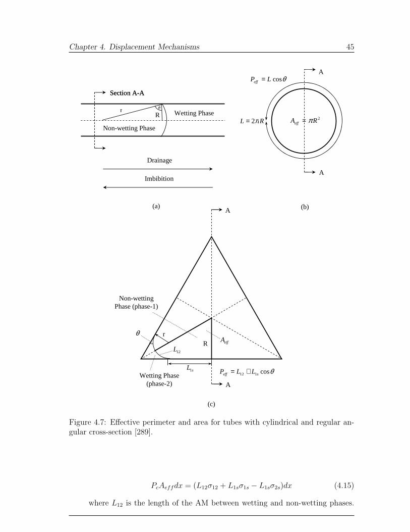
Chapter 4. Displacement Mechanisms 45
(a)
Section A-A
Wetting Phase
Non-wetting Phase
(b)
RL π2= 2RAeff π=
A
A
θcosLPeff =
θr R
Section A-A
Drainage
Imbibition
r effA
sL1
12L
θcos112 seff LLP +=
θ
Non-wetting Phase (phase-1)
Wetting Phase (phase-2)
A
(c)
R
A
Figure 4.7: Effective perimeter and area for tubes with cylindrical and regular an-gular cross-section [289].
PcAeffdx = (L12σ12 + L1sσ1s − L1sσ2s)dx (4.15)
where L12 is the length of the AM between wetting and non-wetting phases.
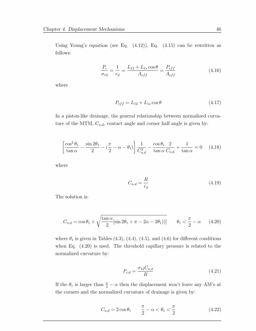
Chapter 4. Displacement Mechanisms 46
Using Young’s equation (see Eq. (4.12)), Eq. (4.15) can be rewritten as
follows:
Pc
σ12
=1
rd
=L12 + L1s cos θ
Aeff
=Peff
Aeff
(4.16)
where
Peff = L12 + L1s cos θ (4.17)
In a piston-like drainage, the general relationship between normalized curva-
ture of the MTM, Cn,d, contact angle and corner half angle is given by:
[cos2 θ1
tan α− sin 2θ1
2− (
π
2− α− θ1)
]1
C2n,d
− cos θ1
tan α
2
Cn,d
+1
tan α= 0 (4.18)
where
Cn,d =R
rd
(4.19)
The solution is:
Cn,d = cos θ1 +
√tan α
2[sin 2θ1 + π − 2α− 2θ1))] θ1 <
π
2− α (4.20)
where θ1 is given in Tables (4.3), (4.4), (4.5), and (4.6) for different conditions
when Eq. (4.20) is used. The threshold capillary pressure is related to the
normalized curvature by:
Pc,d =σ12Cn,d
R(4.21)
If the θ1 is larger than π2− α then the displacement won’t leave any AM’s at
the corners and the normalized curvature of drainage is given by:
Cn,d = 2 cos θ1π
2− α < θ1 <
π
2(4.22)
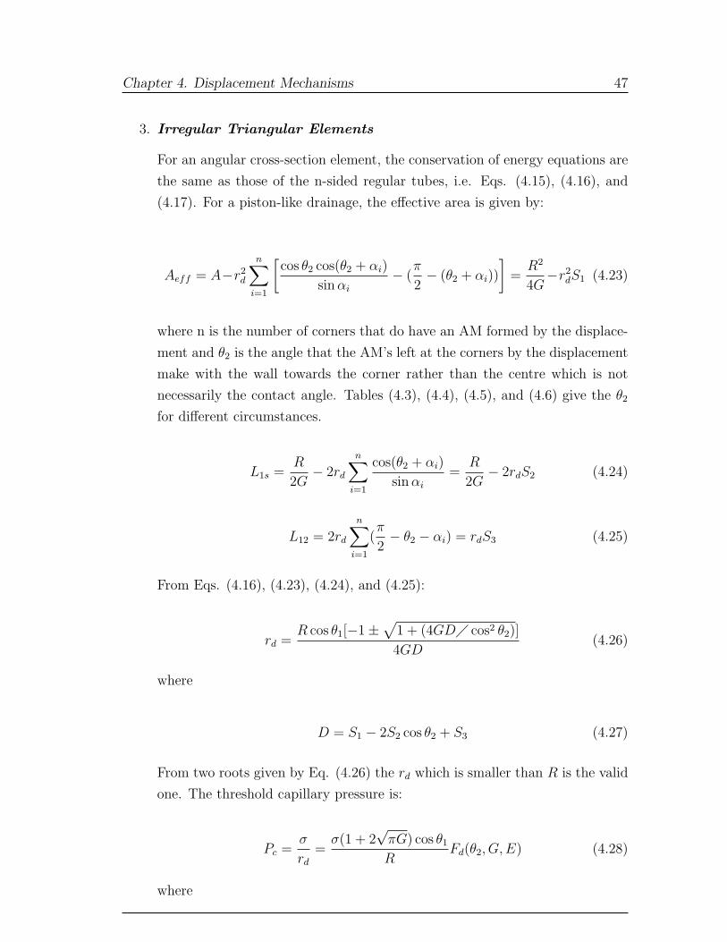
Chapter 4. Displacement Mechanisms 47
3. Irregular Triangular Elements
For an angular cross-section element, the conservation of energy equations are
the same as those of the n-sided regular tubes, i.e. Eqs. (4.15), (4.16), and
(4.17). For a piston-like drainage, the effective area is given by:
Aeff = A−r2d
n∑i=1
[cos θ2 cos(θ2 + αi)
sin αi
− (π
2− (θ2 + αi))
]=
R2
4G−r2
dS1 (4.23)
where n is the number of corners that do have an AM formed by the displace-
ment and θ2 is the angle that the AM’s left at the corners by the displacement
make with the wall towards the corner rather than the centre which is not
necessarily the contact angle. Tables (4.3), (4.4), (4.5), and (4.6) give the θ2
for different circumstances.
L1s =R
2G− 2rd
n∑i=1
cos(θ2 + αi)
sin αi
=R
2G− 2rdS2 (4.24)
L12 = 2rd
n∑i=1
(π
2− θ2 − αi) = rdS3 (4.25)
From Eqs. (4.16), (4.23), (4.24), and (4.25):
rd =R cos θ1[−1±
√1 + (4GD� cos2 θ2)]
4GD(4.26)
where
D = S1 − 2S2 cos θ2 + S3 (4.27)
From two roots given by Eq. (4.26) the rd which is smaller than R is the valid
one. The threshold capillary pressure is:
Pc =σ
rd
=σ(1 + 2
√πG) cos θ1
RFd(θ2, G, E) (4.28)
where
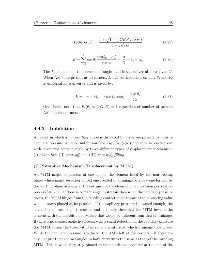
Chapter 4. Displacement Mechanisms 48
Fd(θ2, G, E) =1 +
√1− (4GE� cos2 θ2)
1 + 2√
πG(4.29)
E =3∑
i=1
cos θ2cos(θ2 + αi)
sin αi
− [π
2− θ2 − αi] (4.30)
The Fd depends on the corner half angles and is not universal for a given G.
When AM’s are present at all corners, E will be dependent on only θ2 and Fd
is universal for a given G and is given by:
E = −π + 3θ2 − 3 sin θ2 cos θ2 +cos2 θ2
4G(4.31)
One should note that Fd(θ2 = 0, G, E) = 1 regardless of number of present
AM’s at the corners.
4.4.2 Imbibition
An event in which a non-wetting phase is displaced by a wetting phase at a positive
capillary pressure is called imbibition (see Fig. (4.7)-(a)) and may be carried out
with advancing contact angle by three different types of displacement mechanism:
(I) piston-like, (II) snap-off, and (III) pore-body filling.
(I) Piston-like Mechanism (Displacement by MTM)
An MTM might be present at one end of the element filled by the non-wetting
phase which might be either an old one created by drainage or a new one formed by
the wetting phase arriving at the entrance of the element by an invasion percolation
process [94, 259]. If there is contact angle hysteresis then when the capillary pressure
drops, the MTM hinges from the receding contact angle towards the advancing value
while it stays pinned at its position. If the capillary pressure is lowered enough, the
advancing contact angle is reached and it is only then that the MTM invades the
element with the imbibition curvature that would be different from that of drainage.
If there is no contact angle hysteresis, with a small reduction in the capillary pressure
the MTM enters the tube with the same curvature at which drainage took place.
While the capillary pressure is reduced, the AM’s left at the corners – if there are
any – adjust their contact angles to have curvatures the same as that of the invading
MTM. This is while they stay pinned at their positions acquired at the end of the

Chapter 4. Displacement Mechanisms 49
Table 4.3: Threshold capillary pressures for piston-like and pore-body filling dis-placements with layers of the invading phase contributing to the displacement - oilto water, gas to water and gas to oil.
Item Cross-section Contact Angle Range Equation(s)1 Triangular θij < π
2− α1(1) (4.28)-(4.30)
2 Triangular θij < θextreme(4) & θij ≥ π2− α1 (4.13)
3 Triangular θij ≥ θextreme & θij ≥ π2− α1 (4.34)-(4.41),(4.46),(4.64)-(4.66)
4 Square θij < π4
(4.20)-(4.21)5 Square θij < θextreme & θij ≥ π
4(4.13)
6 Square θij ≥ θextreme & θij ≥ π4
(4.34)-(4.41),(4.43),(4.64)-(4.66)7 Circular 0 ≤ θij ≤ π (4.13)
Item θ1(2) θ2 θ Comment1 θij(3) θij — —2 — — θij —3 (5) π − θij θij Iterative4 θij — — —5 — — θij —6 (5) π − θij θij Iterative7 — — θij —
1. α1 is the half angle of the sharpest corner.
2. θ1 is the contact angle that interface moved with last time.
3. θij = θrij, ij = ow, go, gw - θow = θPD
ow and θgw = θPDgw for displacement of water
by gas and oil during primary drainage respectively.
4. θextreme = π − θ3, where θ3 is calculated using Eqs. (4.47) and (4.44) forelements with triangular and square cross-sections respectively.
5. It can be either π − θ1 or θ1 based on the type of the AM that θ1 belongs to.It is the angle that the AM makes with the surface towards the apex of thecorner.
drainage. The angles may be called hinging. The MTM meets the AM’s with zero
contact angle and the maximum contact angle it reaches before the invasion is the
advancing value. An AM can move only when the hinging contact angle is as large
as the advancing contact angle.
The threshold capillary pressure under which the piston-like imbibition may take
place can be found again using the MS-P theory but the difference with the case
where the theory was applied to find threshold capillary pressure of the drainage is
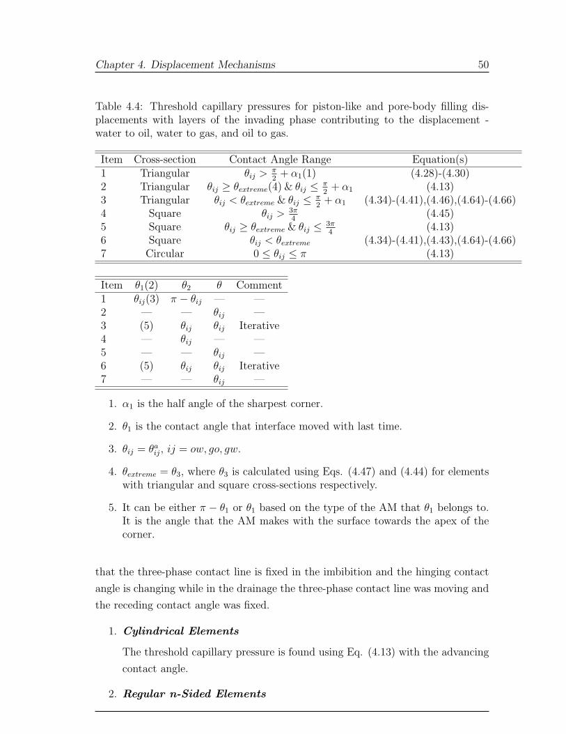
Chapter 4. Displacement Mechanisms 50
Table 4.4: Threshold capillary pressures for piston-like and pore-body filling dis-placements with layers of the invading phase contributing to the displacement -water to oil, water to gas, and oil to gas.
Item Cross-section Contact Angle Range Equation(s)1 Triangular θij > π
2+ α1(1) (4.28)-(4.30)
2 Triangular θij ≥ θextreme(4) & θij ≤ π2
+ α1 (4.13)3 Triangular θij < θextreme & θij ≤ π
2+ α1 (4.34)-(4.41),(4.46),(4.64)-(4.66)
4 Square θij > 3π4
(4.45)5 Square θij ≥ θextreme & θij ≤ 3π
4(4.13)
6 Square θij < θextreme (4.34)-(4.41),(4.43),(4.64)-(4.66)7 Circular 0 ≤ θij ≤ π (4.13)
Item θ1(2) θ2 θ Comment1 θij(3) π − θij — —2 — — θij —3 (5) θij θij Iterative4 — θij — —5 — — θij —6 (5) θij θij Iterative7 — — θij —
1. α1 is the half angle of the sharpest corner.
2. θ1 is the contact angle that interface moved with last time.
3. θij = θaij, ij = ow, go, gw.
4. θextreme = θ3, where θ3 is calculated using Eqs. (4.47) and (4.44) for elementswith triangular and square cross-sections respectively.
5. It can be either π − θ1 or θ1 based on the type of the AM that θ1 belongs to.It is the angle that the AM makes with the surface towards the apex of thecorner.
that the three-phase contact line is fixed in the imbibition and the hinging contact
angle is changing while in the drainage the three-phase contact line was moving and
the receding contact angle was fixed.
1. Cylindrical Elements
The threshold capillary pressure is found using Eq. (4.13) with the advancing
contact angle.
2. Regular n-Sided Elements
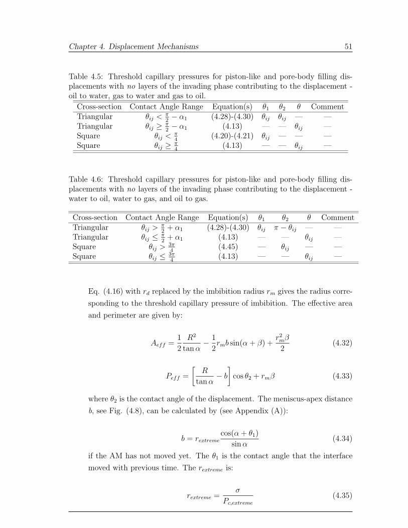
Chapter 4. Displacement Mechanisms 51
Table 4.5: Threshold capillary pressures for piston-like and pore-body filling dis-placements with no layers of the invading phase contributing to the displacement -oil to water, gas to water and gas to oil.
Cross-section Contact Angle Range Equation(s) θ1 θ2 θ CommentTriangular θij < π
2− α1 (4.28)-(4.30) θij θij — —
Triangular θij ≥ π2− α1 (4.13) — — θij —
Square θij < π4
(4.20)-(4.21) θij — — —Square θij ≥ π
4(4.13) — — θij —
Table 4.6: Threshold capillary pressures for piston-like and pore-body filling dis-placements with no layers of the invading phase contributing to the displacement -water to oil, water to gas, and oil to gas.
Cross-section Contact Angle Range Equation(s) θ1 θ2 θ CommentTriangular θij > π
2+ α1 (4.28)-(4.30) θij π − θij — —
Triangular θij ≤ π2
+ α1 (4.13) — — θij —Square θij > 3π
4(4.45) — θij — —
Square θij ≤ 3π4
(4.13) — — θij —
Eq. (4.16) with rd replaced by the imbibition radius rm gives the radius corre-
sponding to the threshold capillary pressure of imbibition. The effective area
and perimeter are given by:
Aeff =1
2
R2
tan α− 1
2rmb sin(α + β) +
r2mβ
2(4.32)
Peff =
[R
tan α− b
]cos θ2 + rmβ (4.33)
where θ2 is the contact angle of the displacement. The meniscus-apex distance
b, see Fig. (4.8), can be calculated by (see Appendix (A)):
b = rextremecos(α + θ1)
sin α(4.34)
if the AM has not moved yet. The θ1 is the contact angle that the interface
moved with previous time. The rextreme is:
rextreme =σ
Pc,extreme
(4.35)
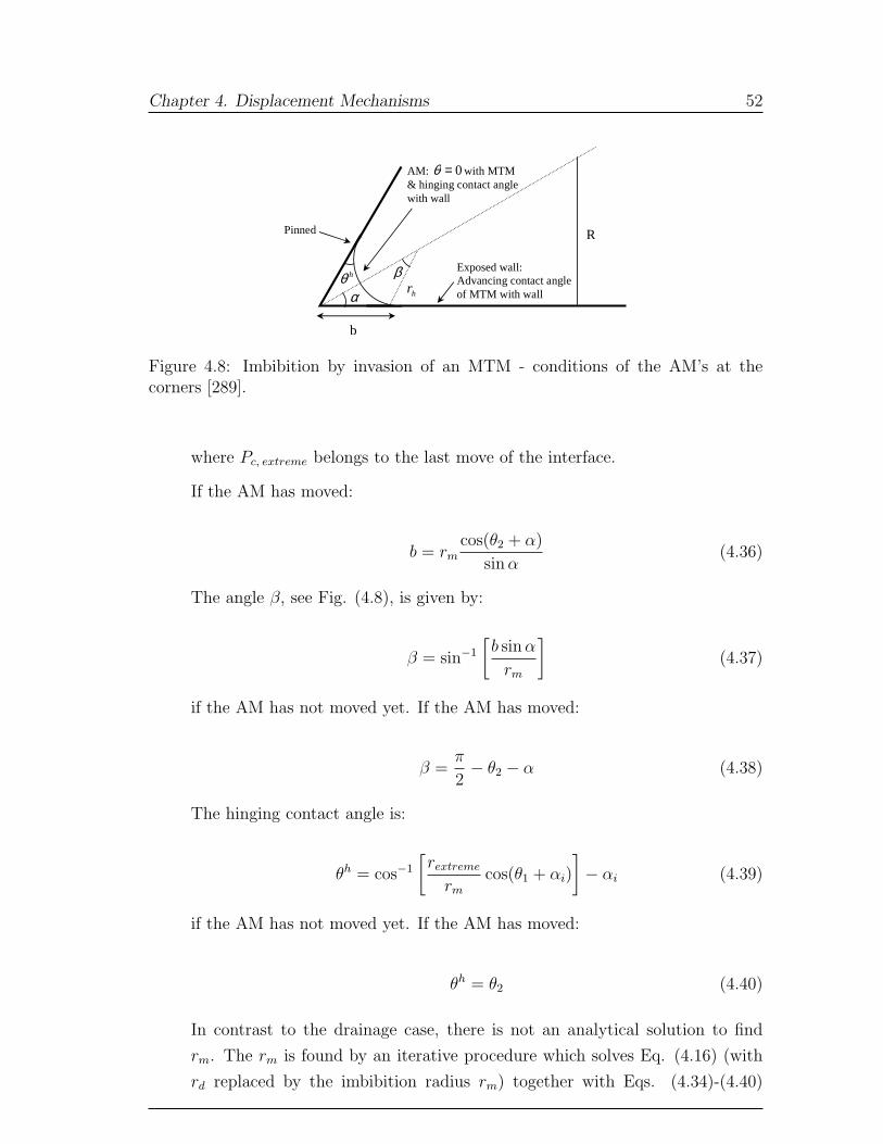
Chapter 4. Displacement Mechanisms 52
α
hθ
R
b
β
hr
Pinned
Exposed wall: Advancing contact angle of MTM with wall
AM: 0=θ with MTM & hinging contact angle with wall
Figure 4.8: Imbibition by invasion of an MTM - conditions of the AM’s at thecorners [289].
where Pc, extreme belongs to the last move of the interface.
If the AM has moved:
b = rmcos(θ2 + α)
sin α(4.36)
The angle β, see Fig. (4.8), is given by:
β = sin−1
[b sin α
rm
](4.37)
if the AM has not moved yet. If the AM has moved:
β =π
2− θ2 − α (4.38)
The hinging contact angle is:
θh = cos−1
[rextreme
rm
cos(θ1 + αi)
]− αi (4.39)
if the AM has not moved yet. If the AM has moved:
θh = θ2 (4.40)
In contrast to the drainage case, there is not an analytical solution to find
rm. The rm is found by an iterative procedure which solves Eq. (4.16) (with
rd replaced by the imbibition radius rm) together with Eqs. (4.34)-(4.40)
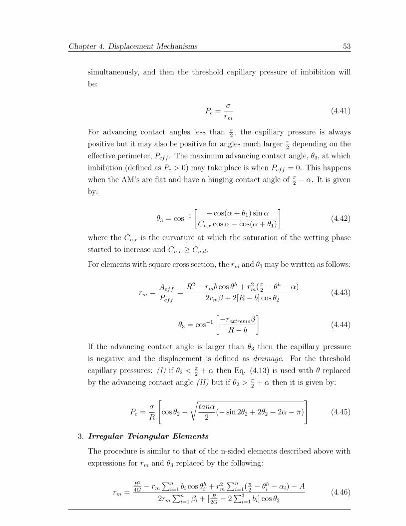
Chapter 4. Displacement Mechanisms 53
simultaneously, and then the threshold capillary pressure of imbibition will
be:
Pc =σ
rm
(4.41)
For advancing contact angles less than π2, the capillary pressure is always
positive but it may also be positive for angles much larger π2
depending on the
effective perimeter, Peff . The maximum advancing contact angle, θ3, at which
imbibition (defined as Pc > 0) may take place is when Peff = 0. This happens
when the AM’s are flat and have a hinging contact angle of π2− α. It is given
by:
θ3 = cos−1
[ − cos(α + θ1) sin α
Cn,r cos α− cos(α + θ1)
](4.42)
where the Cn,r is the curvature at which the saturation of the wetting phase
started to increase and Cn,r ≥ Cn,d.
For elements with square cross section, the rm and θ3 may be written as follows:
rm =Aeff
Peff
=R2 − rmb cos θh + r2
m(π2− θh − α)
2rmβ + 2[R− b] cos θ2
(4.43)
θ3 = cos−1
[−rextremeβ
R− b
](4.44)
If the advancing contact angle is larger than θ3 then the capillary pressure
is negative and the displacement is defined as drainage. For the threshold
capillary pressures: (I) if θ2 < π2
+ α then Eq. (4.13) is used with θ replaced
by the advancing contact angle (II) but if θ2 > π2
+ α then it is given by:
Pc =σ
R
[cos θ2 −
√tanα
2(− sin 2θ2 + 2θ2 − 2α− π)
](4.45)
3. Irregular Triangular Elements
The procedure is similar to that of the n-sided elements described above with
expressions for rm and θ3 replaced by the following:
rm =R2
4G− rm
∑ni=1 bi cos θh
i + r2m
∑ni=1(
π2− θh
i − αi)− A
2rm
∑ni=1 βi + [ R
2G− 2
∑3i=1 bi] cos θ2
(4.46)
Chapter 4. Displacement Mechanisms 54
where n is the number of contributing corners and A is the summation of
corner areas (only those corners that do not have a contributing AM).
θ3 = cos−1[−2rextreme
∑ni=1 βi
R2G− 2
∑3i=1 bi
] (4.47)
or
θ3 = cos−1
[−4G
∑3i=1 cos(θ1 + βi)
(RPc,extreme�σ)− cos θ1 + 12G sin θ1
](4.48)
For drainage: (I) if θ2 < π2
+ α then the threshold capillary pressure is given
by Eq. (4.13) with θ being the advancing contact angle (II) but if θ2 > π2
+ α
then Eqs. (4.28)-(4.30) are used.
(II) Snap-off Mechanism (Displacement by AM’s)
Snap-off corresponds to an imbibition event where the non-wetting phase in the
centre of a pore or throat is displaced by the AM’s of the wetting phase residing in
the corners or layers. This occurs only if there is no MTM present at the entrance
of the element. The AM’s will be present at the corners only if the contact angle
by which the element is drained be less than π2− α otherwise imbibition is possible
only by invasion of an MTM.
If there is no contact angle hysteresis, when the pertinent capillary pressure is
reduced, the AM’s grow and move smoothly towards the centre of the element and
meet to refill the element with the wetting phase.
But if there is contact angle hysteresis, when the relevant capillary pressure
decreases, the invading phase starts swelling and consequently contributing AM’s
- starting from the sharpest corner - may hinge and eventually move - when the
hinging contact angle reaches the advancing value - towards the centre to meet the
other moving or pinned AM’s. When AM’s meet, the centre of the element is filled
spontaneously by the wetting phase. Depending on the magnitude of the advancing
contact angle, snap-off can be spontaneous or forced. When it occurs at a positive
threshold capillary pressure (θa ≤ π2− α1), it is an imbibition event, while it is
forced (drainage) when the threshold capillary pressure is negative (θa > π2− α1).
Snap-off is not favoured over a piston-like or pore-body filling event when there is a
neighbouring element with the invading phase in the centre that is able to carry out
the displacement. The threshold capillary pressures of snap-off events in angular
Chapter 4. Displacement Mechanisms 55
elements with different cross-sectional shape are given next.
1. Regular n-Sided Elements
For spontaneous snap-off the AM’s meet each other when they reach halfway
along the sides of the element. By equating the half length of one side of
the element to the meniscus-apex distance of the moving AM’s, the threshold
capillary pressure is found:
Pc =σ
R[cot α cos θ2 − sin θ2] θ2 ≤ π
2− α (4.49)
But when the snap-off is forced, the threshold capillary pressure is a function
of the curvature of the AM when it starts to move. This is because when the
AM starts to move it can be unstable and may fill the element by the wetting
phase immediately. The threshold capillary pressures are:
Pc =σ
rextreme
cos(θ2 + α)
cos(θ1 + α)θ2 ≤ π − α (4.50)
Pc =σ
rextreme
−1
cos(θ1 + α)θ2 ≥ π − α (4.51)
2. Irregular Triangular Elements
If the snap-off is spontaneous then depending on how large is the advancing
contact angle and whether AM’s are present at all corners, different scenarios,
on which moving AM meets which moving or pinned AM, are imaginable.
These scenarios have different threshold capillary pressures. The event with
the highest capillary pressure is most favourable. They are as follows:
Pc =σ
R
[cos θ2 − 2 sin θ2
cot α1 + cot α2
](4.52)
if the moving AM’s at corners 1 and 2 meet. If the moving AM at the corner
1 meets pinned AM at the corner 2:
Pc =σ(cot α1 cos θ2 − sin θ2)
R(cot α1 + cot α2)− b2
(4.53)
Pc =σ
R
[cos θ2 − 2 sin θ2
cot α1 + cot α3
](4.54)
Chapter 4. Displacement Mechanisms 56
if the moving AM’s at corners 1 and 3 meet. If the moving AM at the corner
1 meets pinned AM at the corner 3:
Pc =σ(cot α1 cos θ2 − sin θ2)
R(cot α1 + cot α3)− b3
(4.55)
Pc =σ
R
[cos θ2 − 2 sin θ2
cot α2 + cot α3
](4.56)
if the moving AM’s at corners 2 and 3 meet. If the moving AM at the corner
2 meets pinned AM at the corner 3:
Pc =σ(cot α2 cos θ2 − sin θ2)
R(cot α2 + cot α3)− b3
(4.57)
If only one corner has a contributing AM, we assume that the element is filled
when the AM moves and meets a noncontributing AM at one of the other
corners.
Pc =σ(cot α1 cos θ2 − sin θ2)
R(cot α1 + cot α3)(4.58)
Pc =σ(cot α1 cos θ2 − sin θ2)
R(cot α1 + cot α2)(4.59)
if only corner 1 has a contributing AM and it meets a noncontributing AM at
corners 3 or 2 respectively.
Pc =σ(cot α2 cos θ2 − sin θ2)
R(cot α2 + cot α3)(4.60)
Pc =σ(cot α2 cos θ2 − sin θ2)
R(cot α2 + cot α1)(4.61)
if only corner 2 has a contributing AM and it meets a noncontributing AM at
corners 3 or 1 respectively.
Pc =σ(cot α3 cos θ2 − sin θ2)
R(cot α2 + cot α3)(4.62)
Pc =σ(cot α3 cos θ2 − sin θ2)
R(cot α1 + cot α3)(4.63)
Chapter 4. Displacement Mechanisms 57
if only corner 3 has a contributing AM and it meets a noncontributing AM at
corners 2 or 1 respectively.
If the contact angle is the same at all corners then Eqs. (4.58) and (4.59) give
the highest capillary pressure when only corner 1 has a contributing AM.
When the snap-off is forced, as soon as the hinging contact angle of the AM at
the sharpest corner becomes as large as the advancing value, it starts moving
towards the centre of the element while the other AM’s are pinned. This means
that the absolute value of the curvature decreases. The AM is not stable and
spontaneously fills the element. The threshold capillary pressure for this case
are given by Eqs. (4.50) and (4.51) where α is corner half angle of the sharpest
corner if AM’s are present at more than one corner.
The equations to compute the threshold capillary pressures for snap-off in two-
and three-phase systems with different wettability conditions are tabulated in Tables
(4.7), and (4.8).
Table 4.7: Threshold capillary pressures for snap-off displacements - oil to water,gas to water and gas to oil.
Cross-section Contact Angle Range Equation(s) θ1(1) θ2 CommentTriangular θij ≥ π
2+ α1 (4.52)-(4.63) — π − θij Min Pc, ij
Triangular θij ≥ α1 & θij ≤ π2
+ α1 (4.50) (2) π − θij —Triangular θij < α1 (4.51) (2) π − θij —Square θij > 3π
4(4.49) — π − θij —
Square θij ≥ π4
& θij ≤ 3π4
(4.50) (2) π − θij —Square θij < π
4(4.51) (2) π − θij —
1. θ1 is the contact angle that interface moved with last time.
2. It can be either π − θ1 or θ1 based on the type of the AM that θ1 belongs to.It is the angle that the AM makes with the surface towards the apex of thecorner.
(III) Pore-body Filling Mechanism
This refers to the displacement of one phase in the centre of a pore by movement
from the centre of adjoining throats(s). For drainage - the displacement of a wetting
phase by non-wetting phase - the threshold capillary pressure is given by similar

Chapter 4. Displacement Mechanisms 58
Table 4.8: Threshold capillary pressures for snap-off displacements - water to oil,water to gas, and oil to gas.
Cross-section Contact Angle Range Equation(s) θ1(1) θ2 CommentTriangular θij ≤ π
2− α1 (4.52)-(4.63) — θij Max Pc, ij
Triangular θij ≤ π − α1 & θij > π2− α1 (4.50) (2) θij —
Triangular θij > π − α1 (4.51) (2) θij —Square θij ≤ π
4(4.49) — θij —
Square θij > π4
& θij ≤ 3π4
(4.50) (2) θij —Square θij > 3π
4(4.51) (2) θij —
1. θ1 is the contact angle that interface moved with last time.
2. It can be either π − θ1 or θ1 based on the type of the AM that θ1 belongs to.It is the angle that the AM makes with the surface towards the apex of thecorner.
expressions for piston-like advance. For imbibition - the displacement of a non-
wetting phase by a wetting phase - the displacement is controlled by the largest
radius of curvature. The threshold capillary pressure depends on inscribed radius
of the pore-body and the number of neighbouring throats that either do not hold
the invading phase in the centre or can not contribute to the displacement as they
might be trapped. For a pore with coordination number m - number of throats
connected to each pore - m−1 pore-body filling events are possible, called In, where
n is the number of neighbouring throats that are not involved in the displacement
1 ≤ n ≤ m − 1 (see Fig. (4.9))[57, 58]. For instance, imagine an oil filled water-
wet circular cross-section pore with 8 throats connected to it. If two of the throats
contain oil in the centre, two gas, one trapped water, and only three continuous
water, then for the water invasion of the pore: n = 2 + 2 + 1 = 5. One should note
that when n = 1, the displacement is a piston-like event with the corresponding
threshold capillary pressures (see sections (4.4.1) and (4.4.2)) [57, 58, 77]. Blunt
[290] and Øren et al. [77] have proposed different empirical models to compute
threshold capillary pressure of the pore-body filling as follows:
Pc =2σ cos θ
Rp
− σ
n∑i=1
eixi (4.64)
Pc =2σ cos θ
Rp +∑n
i=1 eiRt,ixi
(4.65)
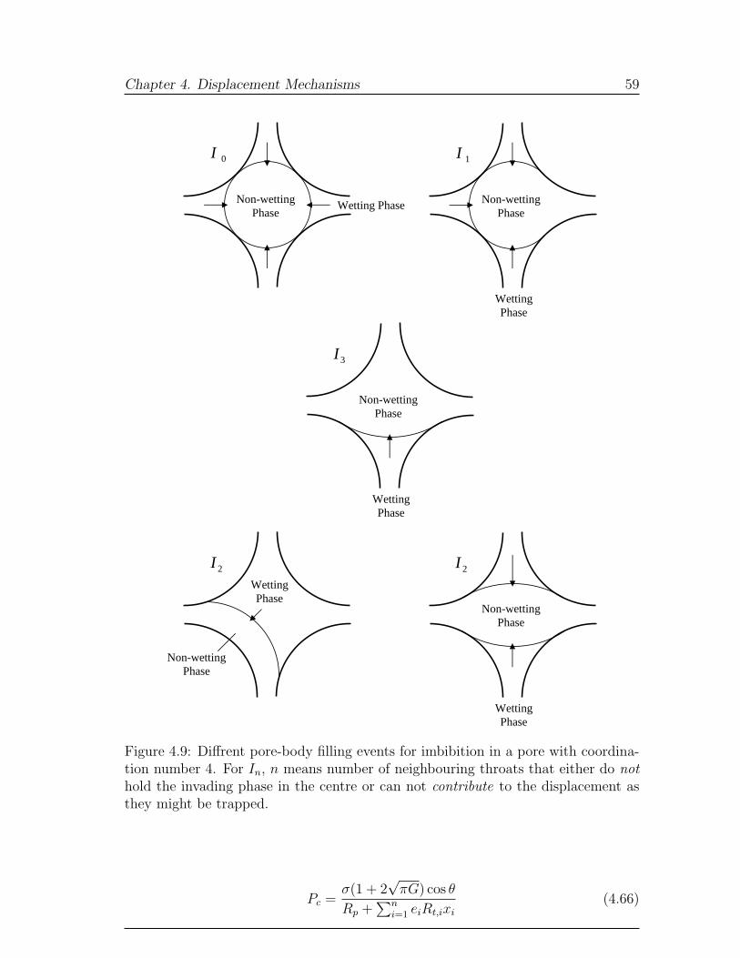
Chapter 4. Displacement Mechanisms 59
2I
Wetting Phase Non-wetting Phase
0I
Wetting Phase
Non-wetting Phase
1I
3I
Wetting Phase
Non-wetting Phase
Wetting Phase
Non-wetting Phase
2I Wetting Phase
Non-wetting Phase
Figure 4.9: Diffrent pore-body filling events for imbibition in a pore with coordina-tion number 4. For In, n means number of neighbouring throats that either do nothold the invading phase in the centre or can not contribute to the displacement asthey might be trapped.
Pc =σ(1 + 2
√πG) cos θ
Rp +∑n
i=1 eiRt,ixi
(4.66)
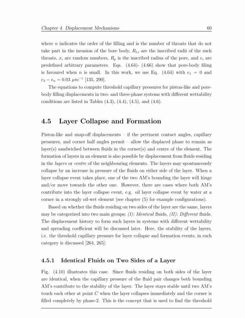
Chapter 4. Displacement Mechanisms 60
where n indicates the order of the filling and is the number of throats that do not
take part in the invasion of the bore body, Rt,i are the inscribed radii of the such
throats, xi are random numbers, Rp is the inscribed radius of the pore, and ei are
predefined arbitrary parameters. Eqs. (4.64)- (4.66) show that pore-body filing
is favoured when n is small. In this work, we use Eq. (4.64) with e1 = 0 and
e2 − en = 0.03 µm−1 [135, 290].
The equations to compute threshold capillary pressures for piston-like and pore-
body filling displacements in two- and three-phase systems with different wettability
conditions are listed in Tables (4.3), (4.4), (4.5), and (4.6).
4.5 Layer Collapse and Formation
Piston-like and snap-off displacements – if the pertinent contact angles, capillary
pressures, and corner half angles permit – allow the displaced phase to remain as
layer(s) sandwiched between fluids in the corner(s) and centre of the element. The
formation of layers in an element is also possible by displacement from fluids residing
in the layers or centre of the neighbouring elements. The layers may spontaneously
collapse by an increase in pressure of the fluids on either side of the layer. When a
layer collapse event takes place, one of the two AM’s bounding the layer will hinge
and/or move towards the other one. However, there are cases where both AM’s
contribute into the layer collapse event, e.g. oil layer collapse event by water at a
corner in a strongly oil-wet element (see chapter (5) for example configurations).
Based on whether the fluids residing on two sides of the layer are the same, layers
may be categorized into two main groups; (I): Identical fluids, (II): Different fluids.
The displacement history to form such layers in systems with different wettability
and spreading coefficient will be discussed later. Here, the stability of the layers,
i.e. the threshold capillary pressure for layer collapse and formation events, in each
category is discussed [264, 265]:
4.5.1 Identical Fluids on Two Sides of a Layer
Fig. (4.10) illustrates this case. Since fluids residing on both sides of the layer
are identical, when the capillary pressure of the fluid pair changes both bounding
AM’s contribute to the stability of the layer. The layer stays stable until two AM’s
touch each other at point C when the layer collapses immediately and the corner is
filled completely by phase-2. This is the concept that is used to find the threshold
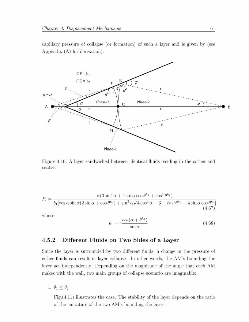
Chapter 4. Displacement Mechanisms 61
capillary pressure of collapse (or formation) of such a layer and is given by (see
Appendix (A) for derivation):
B O
Phase-1
α
α
2hθ
A
r
r
E
C
H
F
απ −
γ
β
Phase-2
φ
ϕ
ψ
Phase-2
r
r
OF = b1
OE = b2
r r
1hθ
Figure 4.10: A layer sandwiched between identical fluids residing in the corner andcentre.
Pc =σ(3 sin2 α + 4 sin α cos θh2 + cos2 θh2)
b1[cos α sin α(2 sin α + cos θh2) + sin2 α√
4 cos2 α− 3− cos2θh2 − 4 sin α cos θh2 ](4.67)
where
b1 = rcos(α + θh1)
sin α(4.68)
4.5.2 Different Fluids on Two Sides of a Layer
Since the layer is surrounded by two different fluids, a change in the pressure of
either fluids can result in layer collapse. In other words, the AM’s bounding the
layer act independently. Depending on the magnitude of the angle that each AM
makes with the wall, two main groups of collapse scenario are imaginable:
1. θ1 ≤ θ2
Fig.(4.11) illustrates the case. The stability of the layer depends on the ratio
of the curvature of the two AM’s bounding the layer:
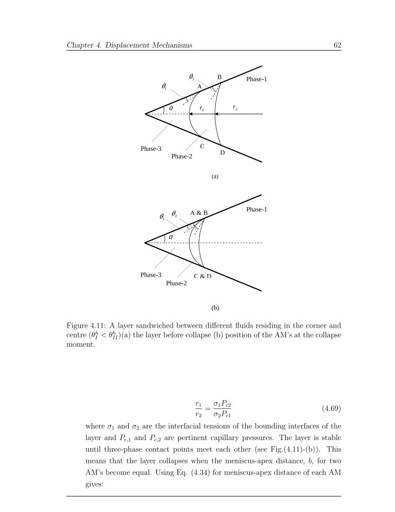
Chapter 4. Displacement Mechanisms 62
(b)
α
Phase-3 Phase-2
Phase-1 A & B
C & D
2θ 1θ
(a)
α 2r
Phase-3 Phase-2
1r
Phase-1
D C
B
A 2θ
1θ
Figure 4.11: A layer sandwiched between different fluids residing in the corner andcentre (θh
I < θhII)(a) the layer before collapse (b) position of the AM’s at the collapse
moment.
r1
r2
=σ1Pc2
σ2Pc1
(4.69)
where σ1 and σ2 are the interfacial tensions of the bounding interfaces of the
layer and Pc,1 and Pc,2 are pertinent capillary pressures. The layer is stable
until three-phase contact points meet each other (see Fig.(4.11)-(b)). This
means that the layer collapses when the meniscus-apex distance, b, for two
AM’s become equal. Using Eq. (4.34) for meniscus-apex distance of each AM
gives:
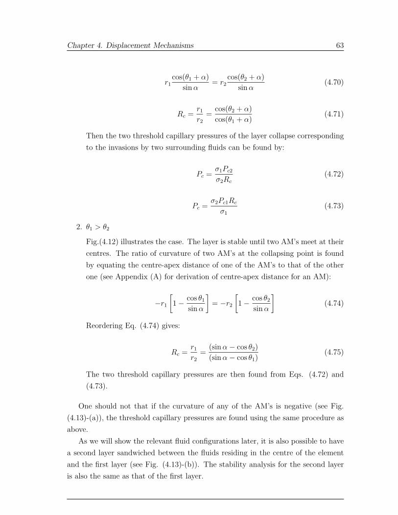
Chapter 4. Displacement Mechanisms 63
r1cos(θ1 + α)
sin α= r2
cos(θ2 + α)
sin α(4.70)
Rc =r1
r2
=cos(θ2 + α)
cos(θ1 + α)(4.71)
Then the two threshold capillary pressures of the layer collapse corresponding
to the invasions by two surrounding fluids can be found by:
Pc =σ1Pc2
σ2Rc
(4.72)
Pc =σ2Pc1Rc
σ1
(4.73)
2. θ1 > θ2
Fig.(4.12) illustrates the case. The layer is stable until two AM’s meet at their
centres. The ratio of curvature of two AM’s at the collapsing point is found
by equating the centre-apex distance of one of the AM’s to that of the other
one (see Appendix (A) for derivation of centre-apex distance for an AM):
−r1
[1− cos θ1
sin α
]= −r2
[1− cos θ2
sin α
](4.74)
Reordering Eq. (4.74) gives:
Rc =r1
r2
=(sin α− cos θ2)
(sin α− cos θ1)(4.75)
The two threshold capillary pressures are then found from Eqs. (4.72) and
(4.73).
One should not that if the curvature of any of the AM’s is negative (see Fig.
(4.13)-(a)), the threshold capillary pressures are found using the same procedure as
above.
As we will show the relevant fluid configurations later, it is also possible to have
a second layer sandwiched between the fluids residing in the centre of the element
and the first layer (see Fig. (4.13)-(b)). The stability analysis for the second layer
is also the same as that of the first layer.
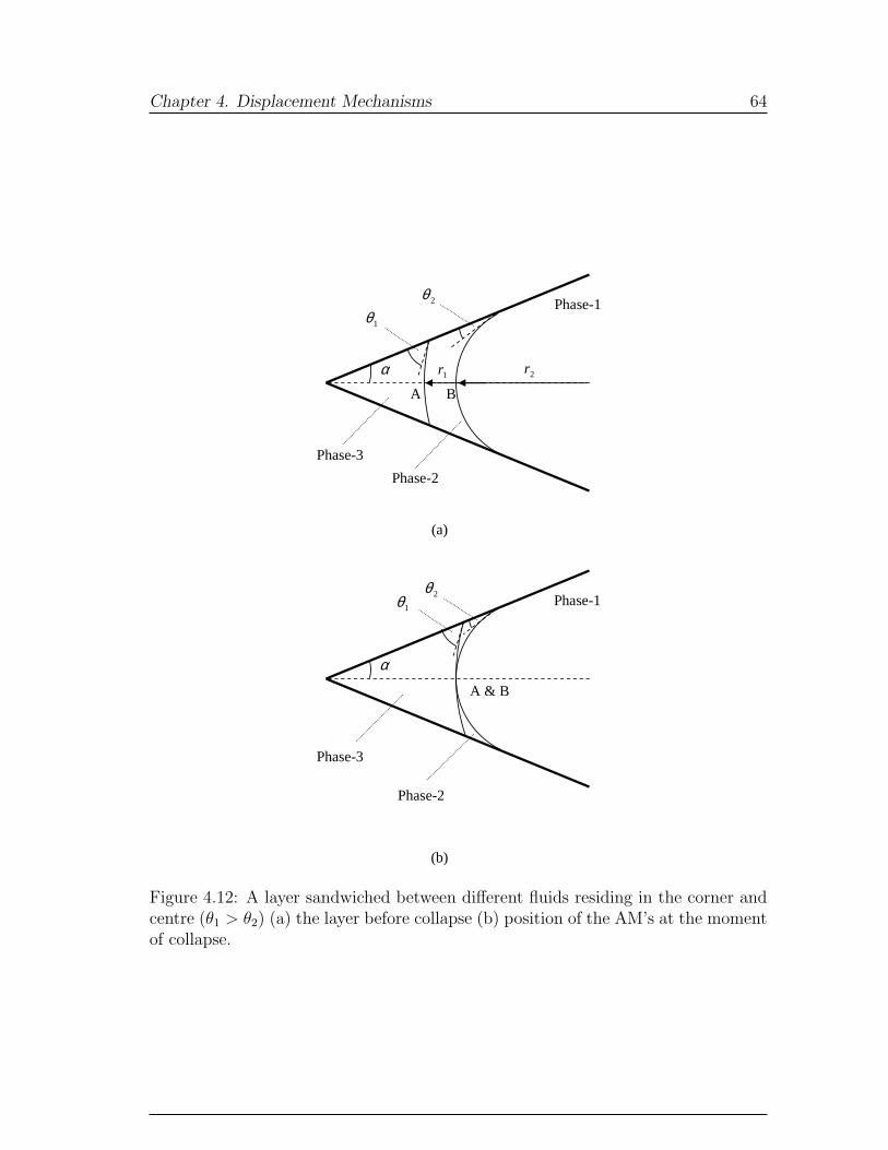
Chapter 4. Displacement Mechanisms 64
Phase-3
Phase-2
Phase-1
2r 1r α
B A
1θ
2θ
(a)
A & B
Phase-3
Phase-2
Phase-1
α
1θ 2θ
(b)
Figure 4.12: A layer sandwiched between different fluids residing in the corner andcentre (θ1 > θ2) (a) the layer before collapse (b) position of the AM’s at the momentof collapse.
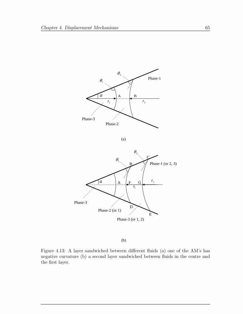
Chapter 4. Displacement Mechanisms 65
A B α
Phase-3 Phase-2
Phase-1
2r 1r
1θ
2θ
(a)
1r A F α
E
D
C
B
Phase-3
Phase-3 (or 1, 2)
Phase-2 (or 1)
Phase-1 (or 2, 3)
G
1θ
2θ
2r
(b)
Figure 4.13: A layer sandwiched between different fluids (a) one of the AM’s hasnegative curvature (b) a second layer sandwiched between fluids in the centre andthe first layer.

Chapter 5
Two- and Three-Phase Fluid
Generic Configurations
Different oil/water, gas/water and gas/oil contact angles and interfacial tensions
make it theoretically possible to accommodate fluids in the corners of the pore
space with different configurations. Figs. (5.1) and (5.2) illustrate all the possible
generic configurations of one, two or three fluids in a single corner of an angular pore
or throat with any values of two- and three-phase contact angles – the whole pore
or throat is composed of no (circle), three (triangular) or four (square) corners. In
all three-phase configurations the constraint among the three-phase contact angles
given by Eq. 2.6 is satisfied. The configurations are equally applicable for any other
angular pore or throat with any number of corners. Altered wettability surfaces are
shown by thicker lines. Fluid located in the corner, layer or centre of a configuration
is called a phase location. For example, configuration group F has three phase
locations, water in a corner, an oil layer and gas in the centre. For single phase
configurations – group A – only one phase location, i.e. water in the centre, is
considered. Every phase location has a flag associated with it indicating whether
the fluid that it accommodates is continuous or trapped. If it is trapped then the
trapped cluster number that the phase location belongs to is also attached to it. A
cluster of phase locations is trapped when it does not connect to the inlet and outlet;
if is does then it is considered continuous. We shall discuss the details of how the
phase locations are assigned to the clusters and how their continuity is determined
later in this work. For elements with a circular cross-section, only one phase may
occupy the pore or throat. For square and triangular cross-sections, the phase in the
middle of the element must be the same for each corner, but different corners may
have different configurations, depending on the corner angle. However, in a single
66
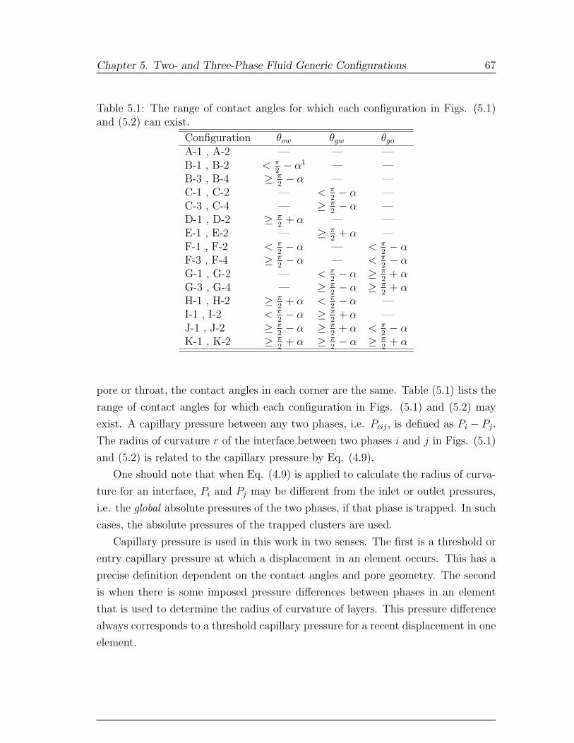
Chapter 5. Two- and Three-Phase Fluid Generic Configurations 67
Table 5.1: The range of contact angles for which each configuration in Figs. (5.1)and (5.2) can exist.
Configuration θow θgw θgo
A-1 , A-2 — — —B-1 , B-2 < π
2− α1 — —
B-3 , B-4 ≥ π2− α — —
C-1 , C-2 — < π2− α —
C-3 , C-4 — ≥ π2− α —
D-1 , D-2 ≥ π2
+ α — —E-1 , E-2 — ≥ π
2+ α —
F-1 , F-2 < π2− α — < π
2− α
F-3 , F-4 ≥ π2− α — < π
2− α
G-1 , G-2 — < π2− α ≥ π
2+ α
G-3 , G-4 — ≥ π2− α ≥ π
2+ α
H-1 , H-2 ≥ π2
+ α < π2− α —
I-1 , I-2 < π2− α ≥ π
2+ α —
J-1 , J-2 ≥ π2− α ≥ π
2+ α < π
2− α
K-1 , K-2 ≥ π2
+ α ≥ π2− α ≥ π
2+ α
pore or throat, the contact angles in each corner are the same. Table (5.1) lists the
range of contact angles for which each configuration in Figs. (5.1) and (5.2) may
exist. A capillary pressure between any two phases, i.e. Pcij, is defined as Pi − Pj.
The radius of curvature r of the interface between two phases i and j in Figs. (5.1)
and (5.2) is related to the capillary pressure by Eq. (4.9).
One should note that when Eq. (4.9) is applied to calculate the radius of curva-
ture for an interface, Pi and Pj may be different from the inlet or outlet pressures,
i.e. the global absolute pressures of the two phases, if that phase is trapped. In such
cases, the absolute pressures of the trapped clusters are used.
Capillary pressure is used in this work in two senses. The first is a threshold or
entry capillary pressure at which a displacement in an element occurs. This has a
precise definition dependent on the contact angles and pore geometry. The second
is when there is some imposed pressure differences between phases in an element
that is used to determine the radius of curvature of layers. This pressure difference
always corresponds to a threshold capillary pressure for a recent displacement in one
element.
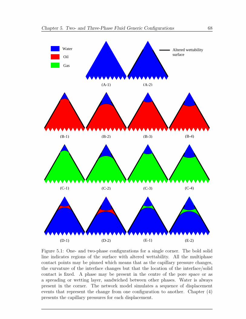
Chapter 5. Two- and Three-Phase Fluid Generic Configurations 68
(A-2) (A-1)
(B-1) (B-2) (B-4) (B-3)
(C-2) (C-1) (C-3) (C-4)
(D-1) (E-1) (E-2) (D-2)
Altered wettability surface
Water
Oil
Gas
Figure 5.1: One- and two-phase configurations for a single corner. The bold solidline indicates regions of the surface with altered wettability. All the multiphasecontact points may be pinned which means that as the capillary pressure changes,the curvature of the interface changes but that the location of the interface/solidcontact is fixed. A phase may be present in the centre of the pore space or asa spreading or wetting layer, sandwiched between other phases. Water is alwayspresent in the corner. The network model simulates a sequence of displacementevents that represent the change from one configuration to another. Chapter (4)presents the capillary pressures for each displacement.
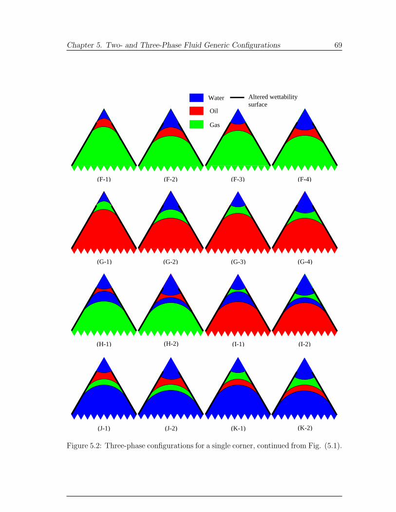
Chapter 5. Two- and Three-Phase Fluid Generic Configurations 69
Altered wettability surface
Water
Oil
Gas
(F-1) (F-2) (F-3) (F-4)
(G-1) (G-2) (G-3) (G-4)
(H-1) (H-2) (I-1) (I-2)
(J-1) (J-2) (K-1) (K-2)
Figure 5.2: Three-phase configurations for a single corner, continued from Fig. (5.1).
Chapter 5. Two- and Three-Phase Fluid Generic Configurations 70
5.1 Definitions
A displacement is defined as a change (see later for details) in generic configuration
groups (indicated by letters in Figs. (5.1) and (5.2)) in an element by an eligible
displacing phase which is the phase residing in a phase location that is topologically
capable of doing the change(s). Based on the type of displacement this can be a
configuration change in one or all corners of the element. For every configuration
change, there might be different ways to carry out the displacement. In such a case
each one is treated as a separate displacement. For instance, imagine configuration
group change F to C due to oil layer collapse (see later for details). The change
could be carried out either by invasion of water in the corner or gas in the centre
which corresponds to a decrease in Pcow or an increase in Pcgo respectively. These two
ways are treated as two separate displacements. A displacement occurs at a thresh-
old capillary pressure. The network model simulates a sequence of displacements
induced by imposed changes in phase pressures.
For every displacement, there are two phase locations associated with it. One
accommodates the displacing fluid of the displacement, the displacing phase location,
and the other one accommodates the displaced fluid, the displaced phase location.
For example, consider configuration group change B to C by an invasion of gas
residing in the centre of a neighbouring pore into oil in the centre of a throat. The
displacing and displaced phase locations for this displacement are the gas centre in
the pore and the oil centre in the throat, respectively.
A process is defined as a consecutive sequence of displacements that involve a
change in the same capillary pressure in the same direction. The change in capillary
pressure, Pcij, is due to injection of either phase i or j. For instance, primary
drainage is a process involving an increase in oil/water capillary pressure. Water
flooding is a different process involving a decrease in oil/water capillary pressure.
Because of contact angle hysteresis, the contact angle can hinge between its
receding and advancing values without the contact line moving and is called the
hinging contact angle. Every interface has two contact angles associated with it:
(I): a target contact angle, which is the contact angle that the new AM’s will have
just after a displacement in that element. The existing (old) AM’s might reach
this value just before displacement. This contact angle may be different from one
process to another. For example, imagine a configuration group change A to B
by oil primary drainage. The new AM’s in configuration group B will have the
target contact angle of θPDow . The target contact angle during water flooding for an
existing oil/water interface in configuration group B is θaow. (II): the furthest contact
Chapter 5. Two- and Three-Phase Fluid Generic Configurations 71
angle, which is the maximum, or minimum, hinging contact angle that an interface
reached during the last process when the pertinent capillary pressure was changing.
This may not necessarily be the same as the target contact angle. For instance,
imagine water flooding is being carried out after primary drainage in a strongly
oil-wet system with θaow = π. When the oil/water capillary pressure decreases the
oil/water AM’s start hinging from θPDow towards the target contact angle (θa
ow). If
water flooding is stopped at some stage then there might be AM’s, particularly in
wide corners, that have not reached the advancing value yet. For such AM’s the last
hinging contact angle is considered as its furthest contact angle. For the AM’s that
reached the target contact angle, the furthest contact angle will be the same as the
target contact angle. For the next process, for instance gas injection, the interface
may start hinging from this furthest value towards the new target contact angle.
Every AM has a meniscus-apex distance, i.e. b (see Fig. (6.5)), associated with
it and is calculated using Eq. (4.34) to be used in area and threshold capillary
pressure calculations. b changes whenever the AM moves.
5.2 Configuration Changes
Configuration changes make it possible to simulate any sequence of fluid injection
in two- and three-phase systems. All possible changes are discussed in this section.
First we present points that one should consider to record configuration changes:
1. After every configuration group change, there will be some new displacements
to be considered. These displacements are added into the appropriate lists
(see details later). For every new displacement, the appropriate list is deter-
mined knowing what phase is displacing and whether the phases occupying
the displacing and displaced phase locations are continuous or trapped.
2. Once a configuration group is changed, the type and the number of AM’s in
the corner may also change. There are two possibilities: (I) the number of
AM’s is the same but the type has been changed – fluid on one side of the AM
has been replaced by a new fluid. For example, consider configuration group
change B to C. In this case the furthest contact angle of the AM before the
configuration change is given to the AM after the configuration change and
then the interface may hinge from its furthest value towards the target contact
angle (due to changes in the pertinent capillary pressure) and ultimately move.
This will prevent any volume error of the fluid residing on the other side of
Chapter 5. Two- and Three-Phase Fluid Generic Configurations 72
the AM – i.e. water in the corner in the example above. We may call this case
an old AM case. (II) the number of AM’s in the corner has either increased
or decreased. If it has increased by piston-like or snap-off displacement then
the new AM will have the furthest contact angle the same as the target value
and moves according to the changes in the relevant capillary pressure. For
example, imagine configuration group change B to F by piston-like invasion
of gas. The furthest contact angle of the new gas/oil AM will be θrgo. If the
number of AM’s has increased by layer formation, see point (4). Finally if
the number of AM’s has decreased (by layer collapse) then it is treated as an
old AM case. An example is the gas layer collapse event by water or oil in
configuration group G to form an oil/water AM in configuration group B.
3. An AM moves once the hinging contact angle becomes as large as the advanc-
ing contact angle of the AM (when the related capillary pressure is decreasing)
or as small as the receding contact angle of the AM (when the related cap-
illary pressure is increasing). Once the AM moves, the new b is calculated.
The value of b is updated as long as the AM keeps moving by changes in the
pertinent capillary pressure in the same direction as when it started to move.
4. When a new layer formation event is considered, one should note that there
are two displacements that may represent such an event and both must be
added to the lists. Imagine an AM where a layer is going to be formed around
it. The first displacement may displace some of the fluid above the AM to
accommodate the layer while the other one displaces some of the fluid below
the AM to make space for the layer. For example, consider gas layer formation
resulting in configuration group change B to G. The two displacements may
take place only if θrgo > π
2+ α. By the first one, gas may displace some of
the water in the corner to open enough space for the layer while forming a
new gas/water interface for which the meniscus-apex distance b is calculated.
Both target and furthest contact angles of the gas/water interface will be θrgw.
One should note that the gas/oil interface, in the new configuration, is treated
as an old AM. π minus the furthest contact angle of the oil/water interface
before the configuration group change is given as the furthest contact angle
of the gas/oil interface. Then the gas/oil interface may start hinging from its
furthest value towards θrgo if the gas/oil capillary pressure is increased during
the process. Also the meniscus-apex distance of the oil/water interface b is
given to the gas/oil interface. The threshold capillary pressure of the layer
Chapter 5. Two- and Three-Phase Fluid Generic Configurations 73
formation is calculated using θrgw and the furthest value of the gas/oil interface.
But by the second displacement, gas may displace some of the oil in the centre
to accommodate itself as a layer. A new gas/oil interface is created and so
its meniscus-apex distance b is calculated. Both target and furthest contact
angles of the gas/oil interface will be θrgo. The gas/water interface is considered
as an old AM and the furthest contact angle of the oil/water interface before
the configuration change is used as the furthest contact angle of the gas/water
interface. Then the gas/water interface may hinge from its furthest value
towards θrgw if the gas/water capillary pressure is increased during the process.
Also the meniscus-apex distance of the oil/water interface b is given to the
gas/water interface. The threshold capillary pressure of the layer formation is
calculated using θrgo and the furthest contact angle of the gas/water interface.
5. Once a displacement changes a configuration group, there might be other dis-
placements that had been considered for the same configuration group change
but through other routes. These displacements are not valid anymore and are
omitted from the lists.
6. New piston-like displacements are considered only if the configuration group
change has replaced the fluid at the centre of the element and there is at least
one different phase residing in the centre of the neighbouring elements.
7. New layer formation displacements are added to the lists only when the phase
that is expected to form the layer is located in neighbouring element(s) in the
centre or layer.
8. New snap-off displacements are added to the list as soon as a new AM is
formed or the type of an old AM has changed. One should note that this is
considered only if the fluid in the centre of the element is residing on one side
of the AM. A new layer collapse event is considered only if a new layer forms.
9. Once a new configuration group is formed, it might allow new displacements
in the neighbouring elements. For instance, imagine a piston-like displacement
by gas changes configuration group B to C in an element. Formation of a gas
layer in the corners, as well as displacement of oil and water in the centre,
of the neighbouring elements are considered if topological and contact angle
circumstances permit.
10. There are some configurations (see Figs. (5.1) and (5.2)) that have more than
one AM. The AM’s and also layers are numbered from the apex inwards.
Chapter 5. Two- and Three-Phase Fluid Generic Configurations 74
New configuration(s) to form by a displacement can be determined knowing the
θow, θgw, and θgo of the displacement and the invading fluid. All changes that can
happen to each configuration group, i.e. displacements, during different two- and
three-phase processes are presented in detail next.
5.2.1 Configuration Group A
An oil layer formation event may change configuration group A to D. Both target
and furthest contact angles of both new oil/water interfaces will be θrow. This may
happen only when θrow ≥ π
2+ α. Since the interfaces are being freshly created, the
meniscus-apex distance (b), which is the same for both interfaces, is calculated. The
new displacements to add are: oil layer collapse by water in the corner, oil layer
collapse by water in the centre, and snap-off of water in the centre by the oil in the
layer. A very similar event by gas, i.e. gas layer formation, may change configuration
group A to E. For both gas/water interfaces, target and furthest contact angles
would be θrgw. For the new interfaces, b is calculated. This may happen only when
θrgw ≥ π
2+ α. The new displacements to add are: gas layer collapse by water in the
corner, gas layer collapse by water in the centre, and the snap-off of water in the
centre by the gas.
Piston like displacement of water by oil may change configuration group A to
B. Both target and furthest contact angles of the oil/water interface would be θrow.
One should note that if oil has not touched the element before, i.e. wettability has
not been altered, then (θow)PD is used instead. The new displacements to add are:
snap-off of oil in the centre by the water in the corner, piston-like displacement of
oil in the centre by the other phases, i.e. gas and/or water, possibly located in the
centre of the neighbouring elements. For the new oil/water interface, b is calculated.
A similar displacement by gas may change configuration group A to C. Both target
and furthest contact angles of the gas/water interface will be θrgw. It should be noted
that if the wettability of the element has not been altered before, then (θgw)PD is
used instead. The new displacements to add are: snap-off of gas in the centre by
water in the corner, piston-like displacement of gas in the centre by the other phases,
i.e. oil and/or water. For the new gas/water interface, b is calculated. Fig. (5.3)-(a)
indicates all the possible configuration changes that might happen to configuration
A.
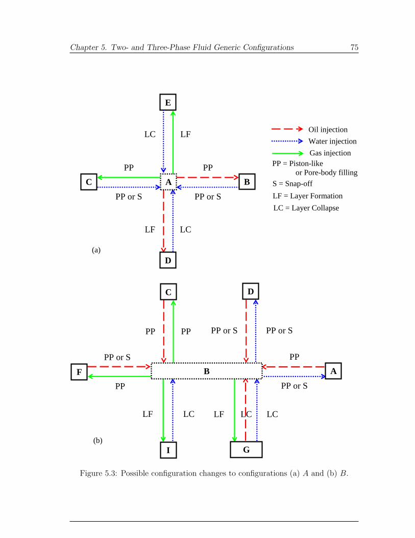
Chapter 5. Two- and Three-Phase Fluid Generic Configurations 75
F
PP or S
PP
PP or S PP or S
D
PP PP
C
A
PP
PP or S
LF LC LC
G I
LF LC
B
C B
E
D
PP
PP or S
PP
PP or S
LF LC
LC LF
A
(a)
(b)
Oil injection
Water injection
Gas injection PP = Piston-like or Pore-body filling
S = Snap-off
LF = Layer Formation
LC = Layer Collapse
Figure 5.3: Possible configuration changes to configurations (a) A and (b) B.

Chapter 5. Two- and Three-Phase Fluid Generic Configurations 76
5.2.2 Configuration Group B
A piston-like or snap-off displacement by water may change configuration group
B to A. The contact angle at which the displacement is carried out is θaow. This
happens only if θaow < π
2+α. No new interfaces are created. The new displacements
to add are: oil layer formation, gas layer formation, and piston-like displacement of
water in the centre by oil and/or gas. If θaow > π
2+ α then a piston-like or snap-off
displacement by water may change configuration group B to D. A new oil/water
interface is formed and so b is calculated. The new displacements to add are: oil
layer collapse by water in the corner, oil layer collapse by water in the centre, snap-
off of water in the centre by the oil in the layer, and piston-like displacement of
water in the centre by oil and/or gas.
A piston-like displacement by gas may change configuration group B to C. The
contact angle to carry out the displacement is θrgo. This may happen only if θr
go >π2− α. The gas/water interface in the new configuration is not considered as a
new interface. It is assigned the b and the furthest contact angle of the oil/water
interface before the configuration change. The interface may hinge from its furthest
contact angles towards θrgw by an increase in gas/water capillary pressure. The new
displacements to add are: snap-off of gas in the centre by the water in the corner,
and piston-like displacement of gas in the centre by water and/or oil. The piston-like
displacement by gas may change the configuration group B to F when θrgo ≤ π
2−α.
A new gas/oil interface is formed for which both target and furthest contact angles
will be θrgo. b is calculated for the gas/oil interface. The new displacements to add
are: oil layer collapse by water in the corner, oil layer collapse by gas in the centre,
snap-off of gas in the centre by the oil in the layer, and piston-like displacement of
gas in the centre by water and/or oil.
A gas layer formation event may change configuration group B to G. The new
displacements to add are: gas layer collapse by water in the corner, gas layer collapse
by oil in the centre, and snap-off oil in the centre by gas in the layer. Gas layer
formation may also change configuration group B to I. The contact angle by which
the displacement is carried out is θrgw. Two new gas/water interfaces are formed and
thus the b that is calculated will be the same for both. Target and furthest contact
angles are θrgw for the new interfaces. This may happen only when θr
gw ≥ π2+α. The
new displacements to add are: the gas layer collapse by water in the corner, the gas
layer collapse by water in the second layer, water layer collapse by gas in the first
layer, water layer collapse by oil in the centre, and snap-off of oil in the centre by
water in the second layer. Fig. (5.3)-(b) shows the possible configuration changes
Chapter 5. Two- and Three-Phase Fluid Generic Configurations 77
to configuration B.
5.2.3 Configuration Group C
A piston-like or snap-off displacement by water may change configuration group C
to A. The contact angle that is used to carry out the displacement is θagw. This
occurs only if θagw < π
2+ α. No new interface is formed. The new displacements
to add are: oil layer formation, gas layer formation, and piston-like displacement of
water in the centre by oil and/or gas. If θagw > π
2+ α then a piston-like or snap-off
displacement by water may change configuration group C to E. A new gas/water
interface is created and thus b is calculated. The new displacements to add are: gas
layer collapse by water in the corner, gas layer collapse by water in the centre and
water and snap-off of water in the centre by gas in the layer.
A piston-like displacement by oil could change configuration group C to B. The
contact angle at which the displacement takes place is θago. This may happen only
if θago < π
2+ α. The oil/water interface is not treated as a new interface. b and
the furthest contact angle of the gas/water interface before the configuration change
are assigned to the oil/water interface. The oil/water interface may hinge from its
furthest value towards θrow due to an increase in oil/water capillary pressure. The
new displacements to add are: snap-off of oil in the centre by the water in the corner,
and piston-like displacement of oil in the centre by water and/or oil. The piston-like
displacement by oil could change the configuration group C to G when θago ≥ π
2+α.
A new gas/oil interface is created and so b is calculated. Both target and furthest
contact angles will be θago. The new displacements to add are: gas layer collapse
by water in the corner, gas layer collapse by oil in the centre, snap-off of oil in the
centre by the gas in the layer, and piston-like displacement of oil in the centre by
water and/or gas.
Oil layer formation could change configuration group C to F . As we described
before, two displacement can cause this change. The two contact angles to be used
are θrow and θa
go. The new displacements to add are: oil layer collapse by water in the
corner, oil layer collapse by gas in the centre, and snap-off of gas in the centre by oil
in the layer. Oil layer formation may also change configuration group C to H. The
contact angle used to carry out the displacement is θrow. The displacement creates
two fresh oil/water interfaces and so the same b is calculated for both. Both target
and the furthest contact angles are θrow for the new interfaces. This may occur only
if θrow ≥ π
2+ α. The new displacements to add are: oil layer collapse by water in
the corner, oil layer collapse by water in the second layer, water layer collapse by
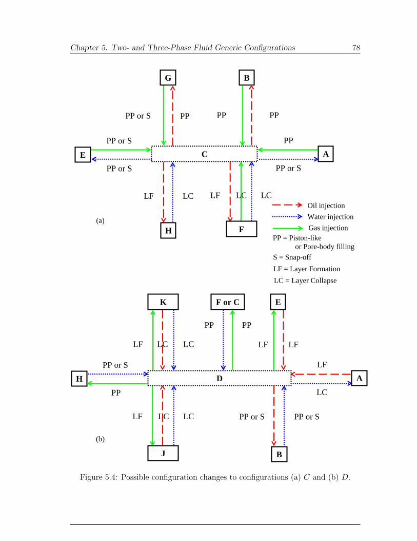
Chapter 5. Two- and Three-Phase Fluid Generic Configurations 78
LF LC LC
F
C A
PP
PP or S
E
PP PP PP
PP or S
PP or S
B G
PP or S
H
LF LC
(a)
(b)
F or C
PP PP
H PP
PP or S
K
LF LC LC
B
PP or S PP or S LF LC LC
J
A
LF
LC
D
E
LF LF
Oil injection
Water injection
Gas injection PP = Piston-like or Pore-body filling
S = Snap-off
LF = Layer Formation
LC = Layer Collapse
Figure 5.4: Possible configuration changes to configurations (a) C and (b) D.
Chapter 5. Two- and Three-Phase Fluid Generic Configurations 79
oil in the first layer, water layer collapse by gas in the centre, and snap-off of gas
in the centre by water in the second layer. Fig. (5.4)-(a) summarizes the possible
configuration changes to configuration group C.
5.2.4 Configuration Group D
An oil layer collapse event by water may change configuration group D to A. The
new displacements to add are: oil layer formation, and gas layer formation.
A piston-like or snap-off displacement by oil may change configuration group
D to B. The contact angle at which the displacement is carried out is θrow. An
oil/water interface is omitted. The contact angle of the oil/water interface in the
corner may hinge from its furthest value to θrow. The new displacements to add are:
snap-off of oil in the centre by water in the corner, two possible gas layer formations
and piston-like displacement of oil in the centre by gas and/or water.
A piston-like displacement by gas may change configuration group D to F . The
contact angle used for the displacement is θrgw. This may happen only if θr
go < π2−α.
The gas/oil interface is not considered as a new interface. The furthest contact angle
and b of the second oil/water interface before the configuration change are assigned
to the gas/oil interface. Then the gas/oil interface may hinge from its furthest
value towards θrgo due to an increase in the gas/oil capillary pressure. The new
displacements to add are: snap-off of gas in the centre by oil in the layer, oil layer
collapse by gas in the centre, water layer formation as a second layer, and piston-
like displacement of the gas in the centre by water and/or oil. If θrgo < π
2− α then
the piston-like displacement may change the configuration D to C. The gas/water
interface is not treated as a new interface and gets the furthest contact angle and
b of the first oil/water interface before the configuration change. The gas/water
interface may then hinge from its furthest value towards θrgw due to an increase in
gas/water capillary pressure. The new displacements to add are: snap-off of gas in
the centre by water in the corner, and piston-like displacement of gas in the centre
by water and/or oil.
A piston-like displacement by gas may convert configuration group D to H. The
contact angle at which the displacement takes place is θrgw which is considered to
be both the furthest and target contact angles for the fresh gas/water interface. b
is calculated. This event happens only if θrgw < π
2− α. The new displacements to
add are: water layer collapse by oil in the first layer, water layer collapse by gas in
the centre, snap-off of gas in the centre by water in the second layer, and piston-like
displacement of gas in the centre by oil and/or water.
Chapter 5. Two- and Three-Phase Fluid Generic Configurations 80
A gas layer formation event may change configuration group D to K. As men-
tioned before, two displacements may carry out such a change. The two contact
angles to use in the two displacements are θrgw and θr
go. This may occur only if
θrgo ≥ π
2+ α. The new displacements to add are: gas layer collapse by water in the
corner, gas layer collapse by oil in the second layer, and oil layer collapse by gas in
the first layer. Gas layer formation may also change configuration group D to J .
The two contact angles applied in two displacements are θrgw and θr
go. The event may
take place only if θrgo ≥ π
2− α and θr
gw ≥ π2
+ α. The new displacements to add are:
gas layer collapse by water in the centre, gas layer collapse by oil in the first layer, oil
layer collapse by gas in the second layer, and snap-off of water in the centre by gas
in the second layer. Fig. (5.4)-(b) summarizes the possible configuration changes to
configuration group D.
5.2.5 Configuration Group E
Gas layer collapse by water could change configuration group E to A. The new
displacements to add are: oil layer formation, and gas layer formation.
A piston-like or snap-off displacement by gas could change configuration group
E to C. The contact angle for the displacement is: θrgw. A gas/water interface is
omitted. The gas/water interface in the corner may hinge from its furthest value
towards θrgw. The new displacements to add are: snap-off of gas in the centre by
water in the corner, two possible oil layer formations, and piston-like displacement
of gas in the centre by oil and/or water.
A piston-like displacement by oil may change configuration group E to I. The
contact angle to use when the displacement is carried out is θrow which is considered
as both the furthest and target contact angles for the new oil/water interface. b is
calculated. The displacement happens only if θrow < π
2− α. The new displacements
to add are: water layer collapse by oil in the centre, water layer collapse by gas
in the first layer, snap-off of oil in the centre by water in the second layer, and
piston-like displacement of oil in the centre by gas and/or water. If θrow ≥ π
2−α and
θago ≥ π
2+α then the piston-like displacement by oil may change configuration group
E to G. The contact angles used for the displacement are θrow and θa
go. The gas/oil
interface is not treated as a new interface. The furthest contact angle and b of the
second gas/water interface before the configuration change are given to the gas/oil
interface. Then the gas/oil interface can hinge from its furthest value towards θago
due to a decrease in gas/oil capillary pressure. The new displacements to add are:
snap-off of oil in the centre by gas in the layer, gas layer collapse by oil in the centre,
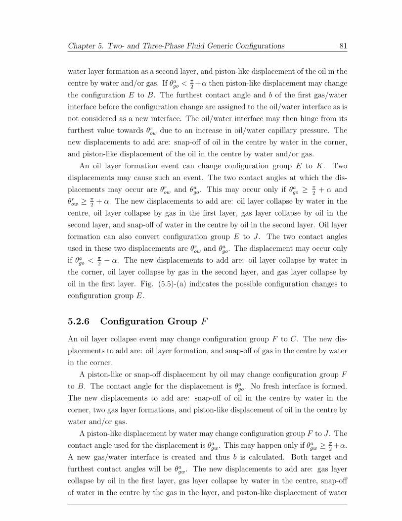
Chapter 5. Two- and Three-Phase Fluid Generic Configurations 81
water layer formation as a second layer, and piston-like displacement of the oil in the
centre by water and/or gas. If θago < π
2+α then piston-like displacement may change
the configuration E to B. The furthest contact angle and b of the first gas/water
interface before the configuration change are assigned to the oil/water interface as is
not considered as a new interface. The oil/water interface may then hinge from its
furthest value towards θrow due to an increase in oil/water capillary pressure. The
new displacements to add are: snap-off of oil in the centre by water in the corner,
and piston-like displacement of the oil in the centre by water and/or gas.
An oil layer formation event can change configuration group E to K. Two
displacements may cause such an event. The two contact angles at which the dis-
placements may occur are θrow and θa
go. This may occur only if θago ≥ π
2+ α and
θrow ≥ π
2+ α. The new displacements to add are: oil layer collapse by water in the
centre, oil layer collapse by gas in the first layer, gas layer collapse by oil in the
second layer, and snap-off of water in the centre by oil in the second layer. Oil layer
formation can also convert configuration group E to J . The two contact angles
used in these two displacements are θrow and θa
go. The displacement may occur only
if θago < π
2− α. The new displacements to add are: oil layer collapse by water in
the corner, oil layer collapse by gas in the second layer, and gas layer collapse by
oil in the first layer. Fig. (5.5)-(a) indicates the possible configuration changes to
configuration group E.
5.2.6 Configuration Group F
An oil layer collapse event may change configuration group F to C. The new dis-
placements to add are: oil layer formation, and snap-off of gas in the centre by water
in the corner.
A piston-like or snap-off displacement by oil may change configuration group F
to B. The contact angle for the displacement is θago. No fresh interface is formed.
The new displacements to add are: snap-off of oil in the centre by water in the
corner, two gas layer formations, and piston-like displacement of oil in the centre by
water and/or gas.
A piston-like displacement by water may change configuration group F to J . The
contact angle used for the displacement is θagw. This may happen only if θa
gw ≥ π2+α.
A new gas/water interface is created and thus b is calculated. Both target and
furthest contact angles will be θagw. The new displacements to add are: gas layer
collapse by oil in the first layer, gas layer collapse by water in the centre, snap-off
of water in the centre by the gas in the layer, and piston-like displacement of water
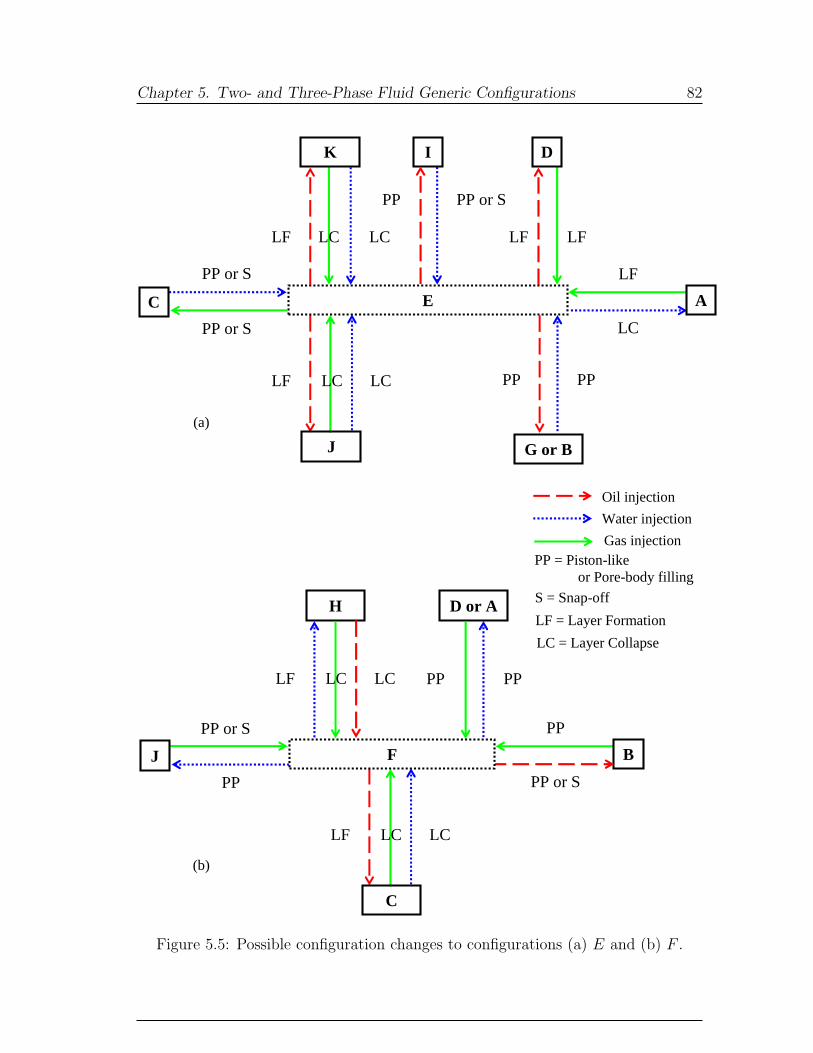
Chapter 5. Two- and Three-Phase Fluid Generic Configurations 82
LF LC LC
C
D or A
B
PP
PP or S
J
PP PP
PP or S
PP
H
LF LC LC
F
(b)
(a)
LF LC LC
J
E A
LF
LC
C
PP or S
PP or S
K
LF LC LC
PP
I
PP or S
G or B
PP PP
D
LF LF
Oil injection
Water injection
Gas injection PP = Piston-like or Pore-body filling
S = Snap-off
LF = Layer Formation
LC = Layer Collapse
Figure 5.5: Possible configuration changes to configurations (a) E and (b) F .
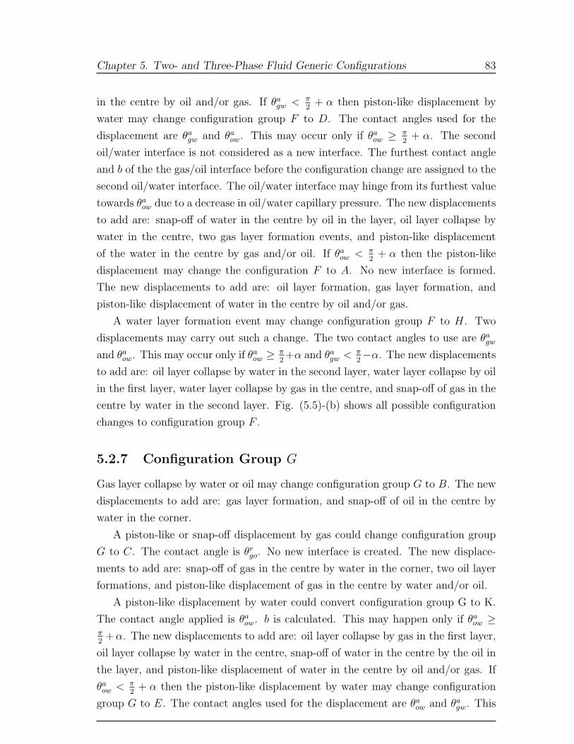
Chapter 5. Two- and Three-Phase Fluid Generic Configurations 83
in the centre by oil and/or gas. If θagw < π
2+ α then piston-like displacement by
water may change configuration group F to D. The contact angles used for the
displacement are θagw and θa
ow. This may occur only if θaow ≥ π
2+ α. The second
oil/water interface is not considered as a new interface. The furthest contact angle
and b of the the gas/oil interface before the configuration change are assigned to the
second oil/water interface. The oil/water interface may hinge from its furthest value
towards θaow due to a decrease in oil/water capillary pressure. The new displacements
to add are: snap-off of water in the centre by oil in the layer, oil layer collapse by
water in the centre, two gas layer formation events, and piston-like displacement
of the water in the centre by gas and/or oil. If θaow < π
2+ α then the piston-like
displacement may change the configuration F to A. No new interface is formed.
The new displacements to add are: oil layer formation, gas layer formation, and
piston-like displacement of water in the centre by oil and/or gas.
A water layer formation event may change configuration group F to H. Two
displacements may carry out such a change. The two contact angles to use are θagw
and θaow. This may occur only if θa
ow ≥ π2+α and θa
gw < π2−α. The new displacements
to add are: oil layer collapse by water in the second layer, water layer collapse by oil
in the first layer, water layer collapse by gas in the centre, and snap-off of gas in the
centre by water in the second layer. Fig. (5.5)-(b) shows all possible configuration
changes to configuration group F .
5.2.7 Configuration Group G
Gas layer collapse by water or oil may change configuration group G to B. The new
displacements to add are: gas layer formation, and snap-off of oil in the centre by
water in the corner.
A piston-like or snap-off displacement by gas could change configuration group
G to C. The contact angle is θrgo. No new interface is created. The new displace-
ments to add are: snap-off of gas in the centre by water in the corner, two oil layer
formations, and piston-like displacement of gas in the centre by water and/or oil.
A piston-like displacement by water could convert configuration group G to K.
The contact angle applied is θaow. b is calculated. This may happen only if θa
ow ≥π2+α. The new displacements to add are: oil layer collapse by gas in the first layer,
oil layer collapse by water in the centre, snap-off of water in the centre by the oil in
the layer, and piston-like displacement of water in the centre by oil and/or gas. If
θaow < π
2+ α then the piston-like displacement by water may change configuration
group G to E. The contact angles used for the displacement are θaow and θa
gw. This
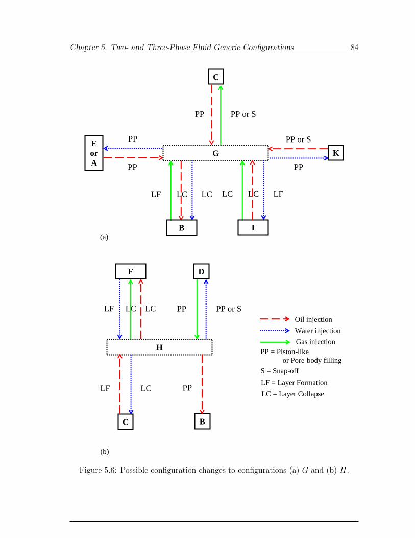
Chapter 5. Two- and Three-Phase Fluid Generic Configurations 84
LF LC LC PP
H
D F
PP or S
LF LC
C B
PP
(b)
(a)
E or A PP PP
PP or S
K
PP
C
PP or S
LF LC LC
B
G
LC LF LC
I
PP
Oil injection
Water injection
Gas injection PP = Piston-like or Pore-body filling
S = Snap-off
LF = Layer Formation
LC = Layer Collapse
Figure 5.6: Possible configuration changes to configurations (a) G and (b) H.
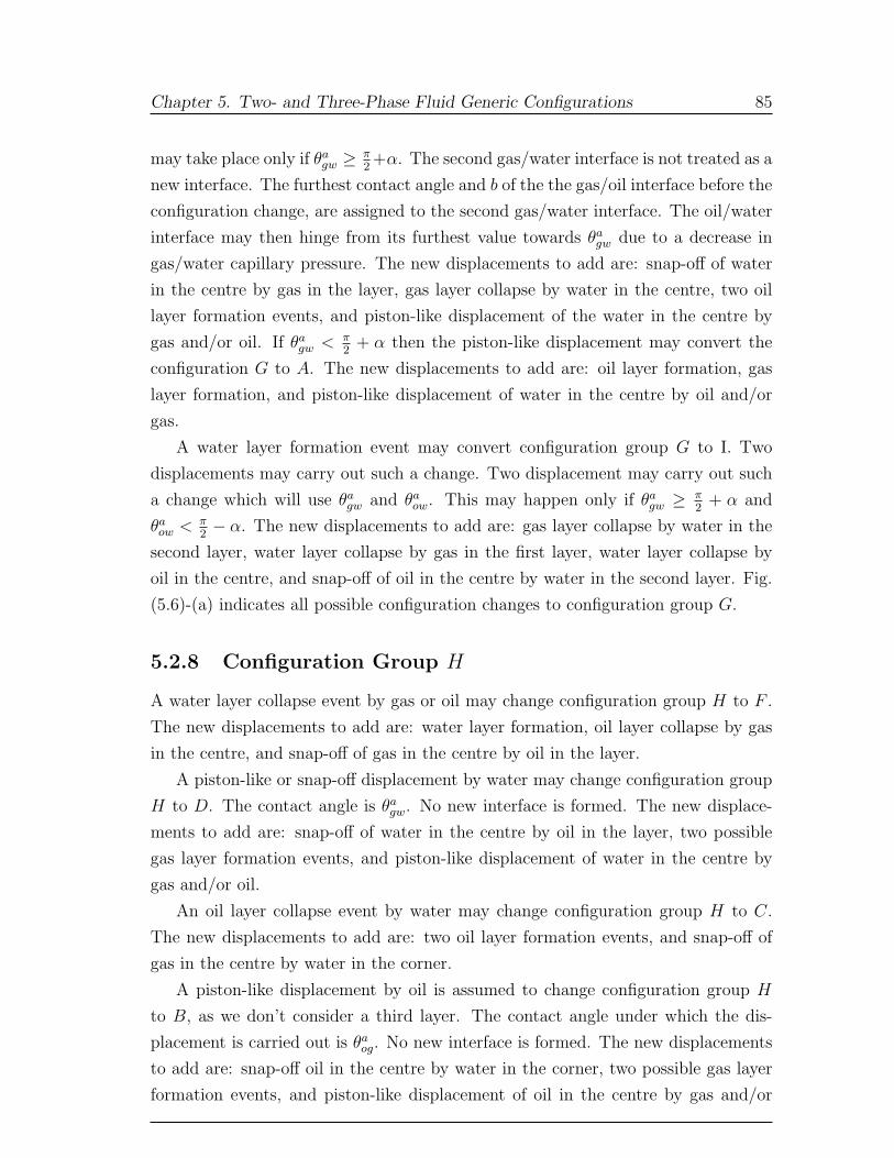
Chapter 5. Two- and Three-Phase Fluid Generic Configurations 85
may take place only if θagw ≥ π
2+α. The second gas/water interface is not treated as a
new interface. The furthest contact angle and b of the the gas/oil interface before the
configuration change, are assigned to the second gas/water interface. The oil/water
interface may then hinge from its furthest value towards θagw due to a decrease in
gas/water capillary pressure. The new displacements to add are: snap-off of water
in the centre by gas in the layer, gas layer collapse by water in the centre, two oil
layer formation events, and piston-like displacement of the water in the centre by
gas and/or oil. If θagw < π
2+ α then the piston-like displacement may convert the
configuration G to A. The new displacements to add are: oil layer formation, gas
layer formation, and piston-like displacement of water in the centre by oil and/or
gas.
A water layer formation event may convert configuration group G to I. Two
displacements may carry out such a change. Two displacement may carry out such
a change which will use θagw and θa
ow. This may happen only if θagw ≥ π
2+ α and
θaow < π
2− α. The new displacements to add are: gas layer collapse by water in the
second layer, water layer collapse by gas in the first layer, water layer collapse by
oil in the centre, and snap-off of oil in the centre by water in the second layer. Fig.
(5.6)-(a) indicates all possible configuration changes to configuration group G.
5.2.8 Configuration Group H
A water layer collapse event by gas or oil may change configuration group H to F .
The new displacements to add are: water layer formation, oil layer collapse by gas
in the centre, and snap-off of gas in the centre by oil in the layer.
A piston-like or snap-off displacement by water may change configuration group
H to D. The contact angle is θagw. No new interface is formed. The new displace-
ments to add are: snap-off of water in the centre by oil in the layer, two possible
gas layer formation events, and piston-like displacement of water in the centre by
gas and/or oil.
An oil layer collapse event by water may change configuration group H to C.
The new displacements to add are: two oil layer formation events, and snap-off of
gas in the centre by water in the corner.
A piston-like displacement by oil is assumed to change configuration group H
to B, as we don’t consider a third layer. The contact angle under which the dis-
placement is carried out is θaog. No new interface is formed. The new displacements
to add are: snap-off oil in the centre by water in the corner, two possible gas layer
formation events, and piston-like displacement of oil in the centre by gas and/or
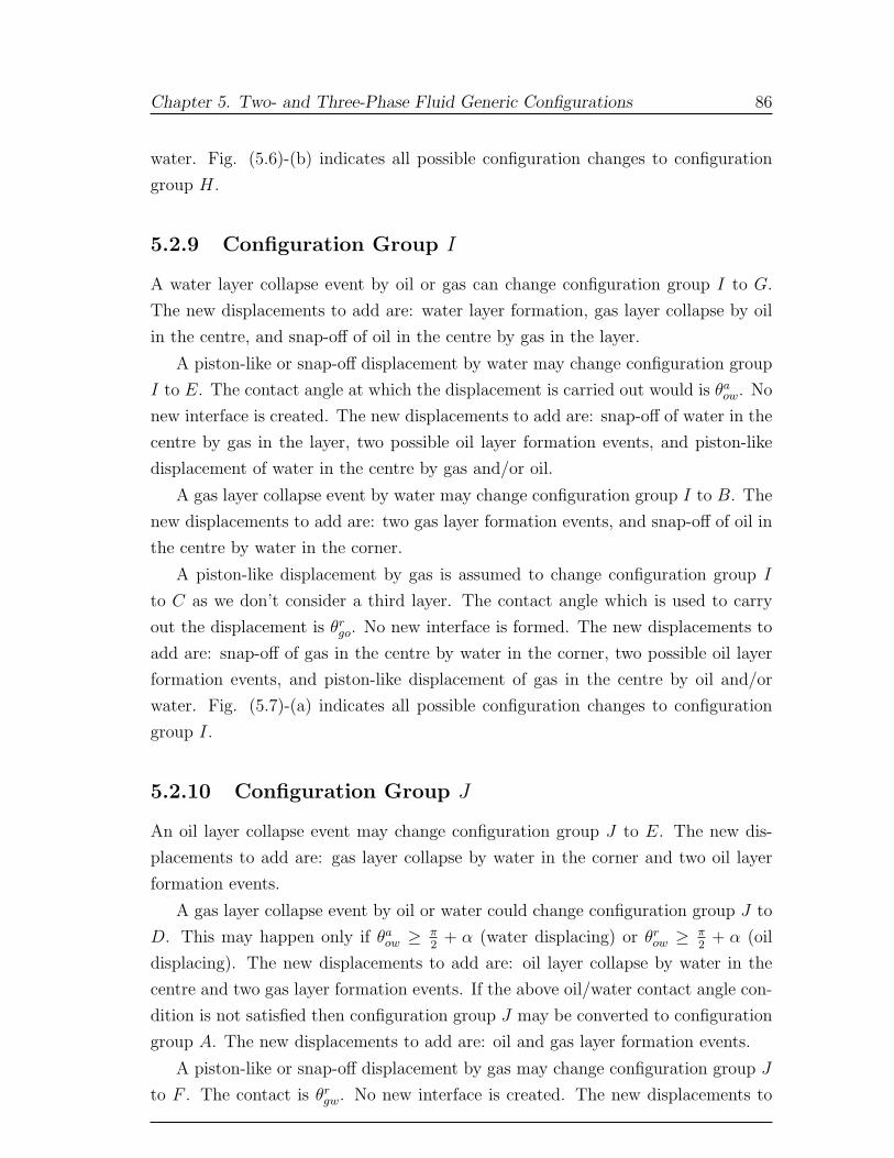
Chapter 5. Two- and Three-Phase Fluid Generic Configurations 86
water. Fig. (5.6)-(b) indicates all possible configuration changes to configuration
group H.
5.2.9 Configuration Group I
A water layer collapse event by oil or gas can change configuration group I to G.
The new displacements to add are: water layer formation, gas layer collapse by oil
in the centre, and snap-off of oil in the centre by gas in the layer.
A piston-like or snap-off displacement by water may change configuration group
I to E. The contact angle at which the displacement is carried out would is θaow. No
new interface is created. The new displacements to add are: snap-off of water in the
centre by gas in the layer, two possible oil layer formation events, and piston-like
displacement of water in the centre by gas and/or oil.
A gas layer collapse event by water may change configuration group I to B. The
new displacements to add are: two gas layer formation events, and snap-off of oil in
the centre by water in the corner.
A piston-like displacement by gas is assumed to change configuration group I
to C as we don’t consider a third layer. The contact angle which is used to carry
out the displacement is θrgo. No new interface is formed. The new displacements to
add are: snap-off of gas in the centre by water in the corner, two possible oil layer
formation events, and piston-like displacement of gas in the centre by oil and/or
water. Fig. (5.7)-(a) indicates all possible configuration changes to configuration
group I.
5.2.10 Configuration Group J
An oil layer collapse event may change configuration group J to E. The new dis-
placements to add are: gas layer collapse by water in the corner and two oil layer
formation events.
A gas layer collapse event by oil or water could change configuration group J to
D. This may happen only if θaow ≥ π
2+ α (water displacing) or θr
ow ≥ π2
+ α (oil
displacing). The new displacements to add are: oil layer collapse by water in the
centre and two gas layer formation events. If the above oil/water contact angle con-
dition is not satisfied then configuration group J may be converted to configuration
group A. The new displacements to add are: oil and gas layer formation events.
A piston-like or snap-off displacement by gas may change configuration group J
to F . The contact is θrgw. No new interface is created. The new displacements to
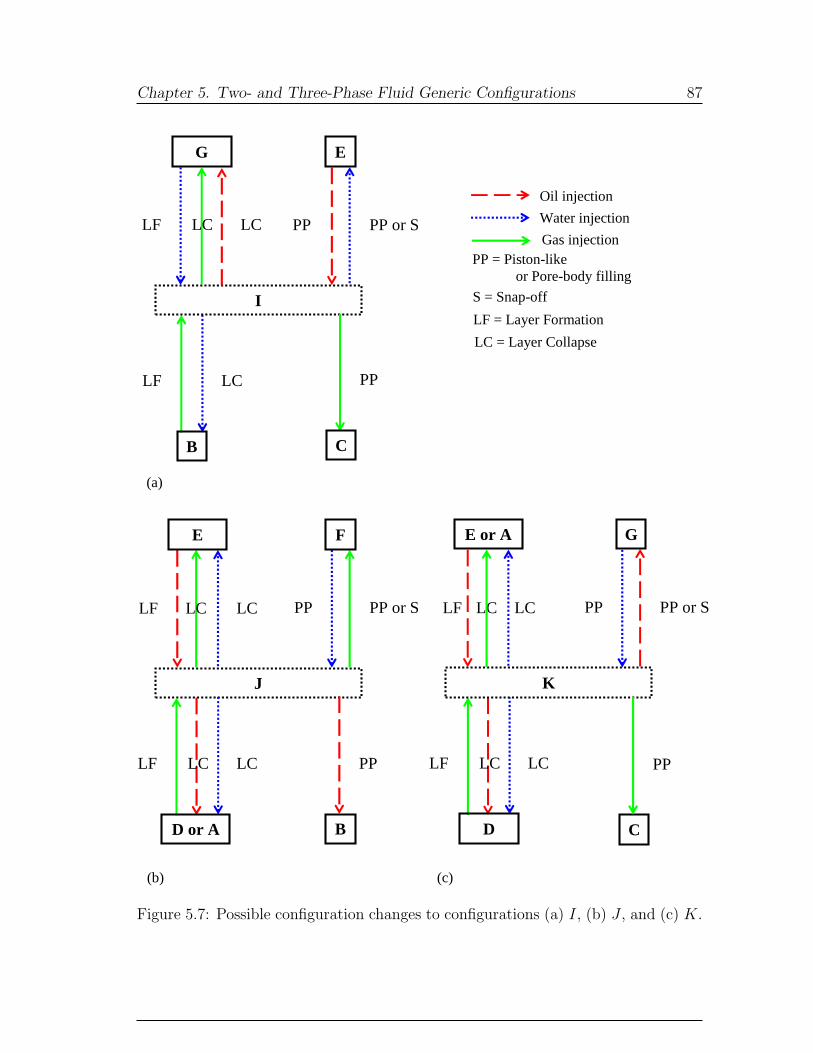
Chapter 5. Two- and Three-Phase Fluid Generic Configurations 87
LF LC
B
PP
I
E G
LF LC LC PP or S
PP
C
(a)
PP
J
F E
LF LC LC PP or S
LF LC LC
D or A
PP
BC
(b)
LF LC LC
D
E or A
LF LC LC PP
K
G
PP or S
PP
CC
(c)
Oil injection
Water injection
Gas injection PP = Piston-like or Pore-body filling
S = Snap-off
LF = Layer Formation
LC = Layer Collapse
Figure 5.7: Possible configuration changes to configurations (a) I, (b) J , and (c) K.
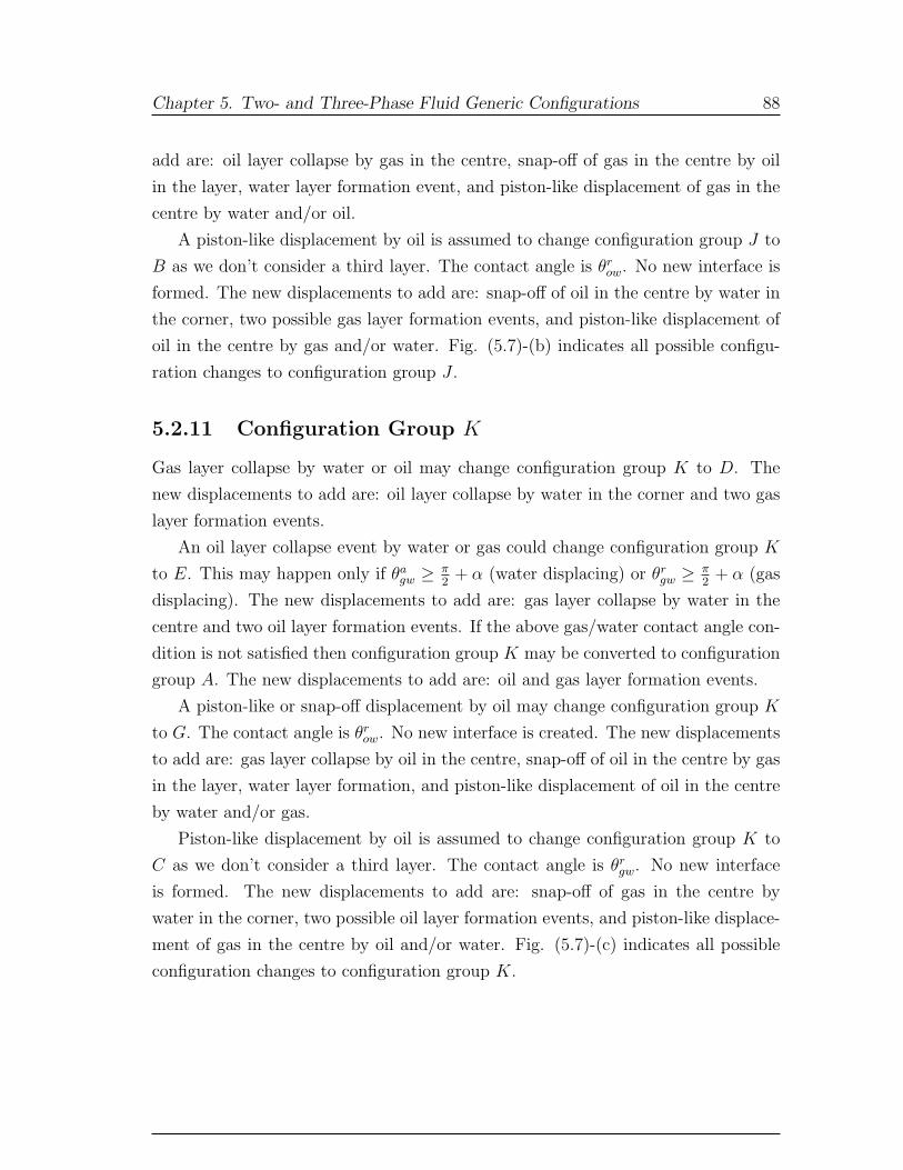
Chapter 5. Two- and Three-Phase Fluid Generic Configurations 88
add are: oil layer collapse by gas in the centre, snap-off of gas in the centre by oil
in the layer, water layer formation event, and piston-like displacement of gas in the
centre by water and/or oil.
A piston-like displacement by oil is assumed to change configuration group J to
B as we don’t consider a third layer. The contact angle is θrow. No new interface is
formed. The new displacements to add are: snap-off of oil in the centre by water in
the corner, two possible gas layer formation events, and piston-like displacement of
oil in the centre by gas and/or water. Fig. (5.7)-(b) indicates all possible configu-
ration changes to configuration group J .
5.2.11 Configuration Group K
Gas layer collapse by water or oil may change configuration group K to D. The
new displacements to add are: oil layer collapse by water in the corner and two gas
layer formation events.
An oil layer collapse event by water or gas could change configuration group K
to E. This may happen only if θagw ≥ π
2+ α (water displacing) or θr
gw ≥ π2
+ α (gas
displacing). The new displacements to add are: gas layer collapse by water in the
centre and two oil layer formation events. If the above gas/water contact angle con-
dition is not satisfied then configuration group K may be converted to configuration
group A. The new displacements to add are: oil and gas layer formation events.
A piston-like or snap-off displacement by oil may change configuration group K
to G. The contact angle is θrow. No new interface is created. The new displacements
to add are: gas layer collapse by oil in the centre, snap-off of oil in the centre by gas
in the layer, water layer formation, and piston-like displacement of oil in the centre
by water and/or gas.
Piston-like displacement by oil is assumed to change configuration group K to
C as we don’t consider a third layer. The contact angle is θrgw. No new interface
is formed. The new displacements to add are: snap-off of gas in the centre by
water in the corner, two possible oil layer formation events, and piston-like displace-
ment of gas in the centre by oil and/or water. Fig. (5.7)-(c) indicates all possible
configuration changes to configuration group K.
Chapter 6
Pore-Scale Network Modelling
6.1 Continuity and Clustering
In pore network modelling of multiphase flow, one of the most important and difficult
tasks to be accomplished is the determination of whether or not a phase location is
trapped as well as keeping this information updated during different processes in a
robust way.
This is vitally important because for every displacement continuity of both dis-
placing and displaced phase locations have to be known a priori (see section (6.4)
for details). Also when it comes to compute the relative permeabilities, continuity of
phase locations must be known as conductances are calculated only for continuous
phase locations. (see section (6.6)).
The algorithm used to determine cluster distributions, critical percolation con-
centration, and percolation probabilities in network modelling was developed by
Hoshen & Kopelman [260] which was later extended to irregular networks by Al-
Futaisi & Patzek [291].
6.1.1 Hoshen & Kopelman Algorithm
The algorithm presented by Hoshen & Kopelman [260] was a method for determining
of cluster distributions, critical percolation concentration and percolation probabil-
ities in a finite lattice. The method was based on a multiple labelling scheme of
members of a cluster in the lattice and was concerned with the determination and
counting of the clusters of a particular type of occupant which were randomly dis-
tributed in a regular lattice of sites. Every site of the lattice was able to hold only
one type of occupant and was connected to its neighbours by bonds. Every site
89
Chapter 6. Pore-Scale Network Modelling 90
holding the particular type of occupant, was assigned a cluster label, mαt , where α
was the name of the cluster. Such a cluster could have several labels as a directory
of natural numbers.
A directory of positive and negative integer numbers was considered where the
positive ones indicated the number of members in each cluster and the negative
ones provided the links between different labels. The directory was updated when
new members were assigned to the existing clusters, new clusters were found or
coalescence occurred. Every new site was assigned a label in one of the following
ways: (I) if there was not any already labelled neighbour with the same occupant,
a new label was used, (II) if there was only one neighbour with the same occupant,
the label of the neighbour was used (III) if there were more than one neighbour with
the same occupant, the smallest label was used. The distinct feature of the multiple
labelling scheme was that a new site could link two or more already labelled cluster
fragments occupied by the same occupant into a bigger cluster without relabelling
them. The algorithm was able to label the sites, find the clusters, and count them
by a single scan of the lattice.
6.1.2 Displacement Based Algorithm
We use a new algorithm whose principles are described below. It is applicable to
any two- or three-dimensional regular and random network with any number of
phases, i.e. phase locations, residing in a pore or throat. In contrast, the original
Hoshen-Kopelman algorithm [260] assumed that only a single phase occupied each
element. Our algorithm, as we will discuss in detail shortly, is also different from the
extension of Hoshen-Kopelman algorithm by Al-Futaisi & Patzek [291] since we do
not – except for the first time – scan the entire network to update our information
regarding the continuity status of different phases residing in every element.
First, the network at its initial condition is scanned to determine continuity of
all its present phase locations. Flags are assigned to every single phase location
indicating if it is continuous or trapped. If a phase location is trapped then the
cluster number which it belongs to is also attached to it. To scan the network the
algorithm shown in Fig. (6.1) is used. The algorithm uses Table (6.1) that lists
the circumstances under which phase locations holding the same phase in adjacent
pores and throats are considered connected. One should note that we assume that
within a single pore or throat all the corners are connected and so are all the layers
holding the same phase. This definition of connectivity is used to define clusters of
each phase. During the scanning process, if a trapped cluster is found then all phase
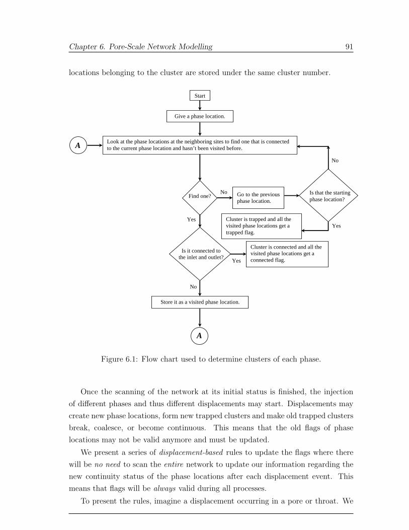
Chapter 6. Pore-Scale Network Modelling 91
locations belonging to the cluster are stored under the same cluster number.
A
Go to the previous phase location.
Is it connected to the inlet and outlet?
A
Cluster is connected and all the visited phase locations get a connected flag.
Yes
Store it as a visited phase location.
No
Yes
No
Look at the phase locations at the neighboring sites to find one that is connected to the current phase location and hasn’t been visited before.
Find one?
Yes Cluster is trapped and all the visited phase locations get a trapped flag.
No
Start
Give a phase location.
Is that the starting phase location?
Figure 6.1: Flow chart used to determine clusters of each phase.
Once the scanning of the network at its initial status is finished, the injection
of different phases and thus different displacements may start. Displacements may
create new phase locations, form new trapped clusters and make old trapped clusters
break, coalesce, or become continuous. This means that the old flags of phase
locations may not be valid anymore and must be updated.
We present a series of displacement-based rules to update the flags where there
will be no need to scan the entire network to update our information regarding the
new continuity status of the phase locations after each displacement event. This
means that flags will be always valid during all processes.
To present the rules, imagine a displacement occurring in a pore or throat. We

Chapter 6. Pore-Scale Network Modelling 92
Table 6.1: Criteria for connectivity of phase locations holding the same phase inadjacent pores and throats.
Phase location(1) Phase location(2) Connected?Corner Corner YesCorner Layer NoCorner Centre NoLayer Layer YesLayer Centre YesCentre Centre Yes
may call that pore or throat the target element which may have several neighbours.
For a pore, the neighbours are the throats connected to it and for the throats, the
pores. Neighbours do not necessarily contain the same fluid as the target element.
Every phase location in the target element and its neighbours is considered as a
member of a chain of phase locations with the same phase and will act as a head.
If a chain stretches to the inlet and outlet, it is continuous, otherwise it is a trapped
cluster.
The rules are itemized as follows:
1. Before the displacement takes place, all the chain heads in the target element
and its neighbours are determined (i.e. separately in each pore and throat). For
instance in a corner of an element with configuration group F , see Fig. (5.2),
three chain heads, i.e. water corner, oil layer, and gas centre, are determined.
One should note that at this stage, there is no need to know how far the chains
stretch. Similar phase locations in an element will be members of the same
chain and either of them could be used as the chain head. For example, in an
element with triangular cross-section with all the corners having configuration
group G, all the gas layers are considered as members of a gas chain and
obviously should all have the same flags and only one of them is used as a chain
head. This is also the case for the water corners. However, phase locations
with the same phase but in a different type of location might not necessarily be
considered as members of the same chain. For instance, in configuration group
D, water in the centre is not considered as a member of the chain that the
water corner is a member of, unless they touch each other in a corner where
there is no oil layer. The water centre is considered as a head of another water
chain.
2. Before the displacement, the connectivity of chain heads in the target element
Chapter 6. Pore-Scale Network Modelling 93
with the chain heads in its neighbours are determined and stored using the
criteria listed in Table (6.1).
3. The displacement is carried out which may omit some old phase locations
while forming new ones in the target element. Only for the newly formed
phase locations must flags be assigned. The new phase locations created by
piston like, snap-off, and layer formation displacement events that hold the
same phase as the displacing phase location will get flags exactly the same as
those of the displacing phase location. For instance, for oil from the centre of
a neighbour that creates an oil layer in the target element, the newly formed
oil layer will get the same flags as the oil in the centre. But if the newly born
phase location contains a phase similar to that of the displaced phase location,
i.e. old, then it will get the same flags as the displaced phase location. For
example, consider configuration group change B to F. The oil layers will get
flags the same as those of oil in the centre before the displacement.
4. If the displacing phase location is trapped and forms new phase locations with
the same flags then the new phase locations are added to the trapped cluster
as new members.
5. If the displaced phase location was trapped and after the displacement it does
not exist anymore, it is omitted from the list of the trapped cluster members.
6. If the target element is connected directly to the inlet or outlet and the new
phase location is formed by the phase invading from the outside of the network,
a continuous flag is assigned to the new phase location.
7. After the displacement, new possible chain heads are determined in the target
element.
8. Connectivity of the new chain heads in the target elements with the chain
heads in the neighbours are determined and stored.
9. Connectivity of every single chain head in the neighbours to the chain heads
with the same phase in the target element before and after displacement are
compared. If a chain head was disconnected (or connected) to the target
element before the displacement and stays disconnected (or connected) after
the displacement, there is no need to change the flags of the chain.
Chapter 6. Pore-Scale Network Modelling 94
10. If a chain head in a neighbour was connected to the target element before
the displacement and got disconnected after the displacement then: (I) If
the chain head was continuous then its continuity is checked using the algo-
rithm presented in Fig. (6.1) as the chain might have got trapped due to the
disconnection from the target element. (II) If the chain head was trapped,
disconnection from the target element might mean that a trapped cluster has
broken into two or more smaller trapped clusters. This is called a local break
and the next point describes how the algorithm realizes if a local break has
actually broken the displaced trapped cluster into smaller ones.
11. In order to find if a local break is a break, one of the phase locations residing in
a neighbour that belongs to the displaced (mother) trapped cluster is chosen.
Then all the phase locations connected to it are found using the algorithm
presented in Fig. (6.1). If all the other phase locations residing in the neigh-
bour(s) that belong to the mother trapped cluster are among the found phase
locations, then the disconnection has been only a local one and not a break.
If not, it is a break and the found phase locations form a new trapped cluster
with a new identity. Now all the other phase locations in the neighbour(s)
that were members of the mother trapped cluster are also picked up one by
one and all the connected phase locations are found and the process continues
exactly the same as for the first phase location until there is no any phase
location left that has not been assigned to a new smaller trapped cluster.
12. If a chain head in a neighbour was disconnected from the target element before
the displacement and has become connected after the displacement then: (I)
If the chain in the neighbour was trapped while the chain head in the target
element is continuous then the trapped cluster has become continuous and
flags of all its members are changed to continuous. The opposite case is also
possible when the chain head in the target element is trapped while the one
in the neighbour was continuous. (II) If the chain head in the neighbour was
trapped and so was the chain head in the target element that it got connected
to, then a coalescence has happened and both trapped clusters now will form
a bigger trapped cluster (see section (6.3.1) for details). For all other cases
there is no need to change the flags of the chains.
Chapter 6. Pore-Scale Network Modelling 95
6.2 How to Choose the Right Displacement
Based on what phase displaces what phase, there are six possible two-phase pro-
cesses: oil displacing water which is controlled by an increase in Pcow. This could be
done either by an increase in oil pressure or a decrease in water pressure. Likewise,
water displacing oil (decrease in Pcow ≡ increase in water pressure or decrease in
oil pressure), gas displacing water (increase in Pcgw ≡ increase in gas pressure or
decrease in water pressure), water displacing gas (decrease in Pcgw ≡ increase in
water pressure or decrease in gas pressure), gas displacing oil (increase in Pcgo ≡increase in gas pressure or decrease in oil pressure), and oil displacing gas (decrease
in Pcgo ≡ increase in oil pressure or decrease in gas pressure). Every displacement
belongs to one or two of these six processes. For instance, collapse of the gas layer
which leads to configuration group change G to B could occur by either water or oil
invasion which corresponds to a decrease in Pcow or Pcgo, respectively. This means
that this displacement belongs to both water displacing gas and oil displacing gas
processes. But, for example, configuration group change B to A only belongs to a
water displacing oil process.
A process can be carried out either by increasing the pressure of the displacing
fluid or decreasing the pressure(s) of the displaced fluid(s). In two-phase processes,
both methods may produce the same results but that may not necessarily be the
case for three-phase systems. In this work, we shall model all the processes by
increasing the pressure of the injection fluid. For example, gas injection into water
and oil is carried out by increasing the gas pressure not by decreasing the pressures
of oil and water.
For every single displacement, a threshold capillary pressure is calculated – see
chapter (4) – which might depend on the relevant contact angles, corner angles
and inscribed radius of the element of interest, other capillary pressures and the
configuration of nearest neighbour pores and throats. Then depending on what
fluid is displacing and what is displaced, the threshold absolute pressure of the
displacing fluid for a single displacement is found from:
P thresholdi = P threshold
cij + Pj (6.1)
or
P thresholdj = Pi − P threshold
cij (6.2)
where Pi and Pj are pressures of phases i and j, respectively. The pressure of a
Chapter 6. Pore-Scale Network Modelling 96
fluid is referred to the pressure of a continuous cluster of that fluid and is assumed
to be the same as the inlet or outlet pressure of the fluid. There might be several
such clusters of one fluid but they all will have the same pressure. The foregoing
procedure is used for single displacements where one continuous phase location dis-
places another continuous one. When one or both of them is trapped, P thresholdi and
P thresholdj are found in a slightly different way that shall be discussed in the Multiple
Displacements section (6.4). Threshold pressures of all the displacements that have
the same displacing fluid are ranked into the same main sorted list. Consequently,
in three-phase systems there will be three main sorted lists for gas, oil and water as
displacing phases. This means that every list may include entries from two different
processes with the same displacing fluid. For instance, the water list may include
threshold pressures from water displacing oil and water displacing gas processes.
Initially when the network is water-filled, only oil or gas can be injected and
the only processes are those that displace water by oil or gas from the elements
connected to the inlet. From this stage onwards, new displacements must be added,
if there were any, to the appropriate list(s) regardless of whether they could occur
during the current process or not (see chapter 5 for details). The exact configuration
change associated with these new displacements may not be clear at this stage; and
it is not necessary, as they may occur during other processes when the conditions,
i.e. pressures and target contact angles, will be different. Before a new displacement
is added to an appropriate list, its threshold capillary pressure is calculated. Before
a new displacement is added to a main sorted list, it must be checked to see if both
displacing and displaced phase locations are continuous. If one or both of them is
trapped, then, based on what fluid is displacing and what fluid is displaced, the
displacement is added into an appropriate sorted sublist in one of the 18 multiple
displacement search categories tabulated in Tables (6.2), (6.3) and (6.4) (see details
in Multiple Displacements section (6.4)). If both phase locations are continuous
then it is added to an appropriate main sorted list.
By knowing the injection fluid, the relevant main sorted list is selected, for
example the water list for water injection. The list is sorted in ascending order.
Imagine the invading fluid is i. This means that we consider a displacement event
where the volume of i in an element increases. Phase i can invade either phase j or
k. The threshold pressure at the top of the list belongs to the most favorable, i.e.
easiest, displacement. This could be displacement of j or k by i. If the displacement
is valid then it takes place. A displacement is valid when the displacing and displaced
phase locations are present and their continuity status flags are consistent with the
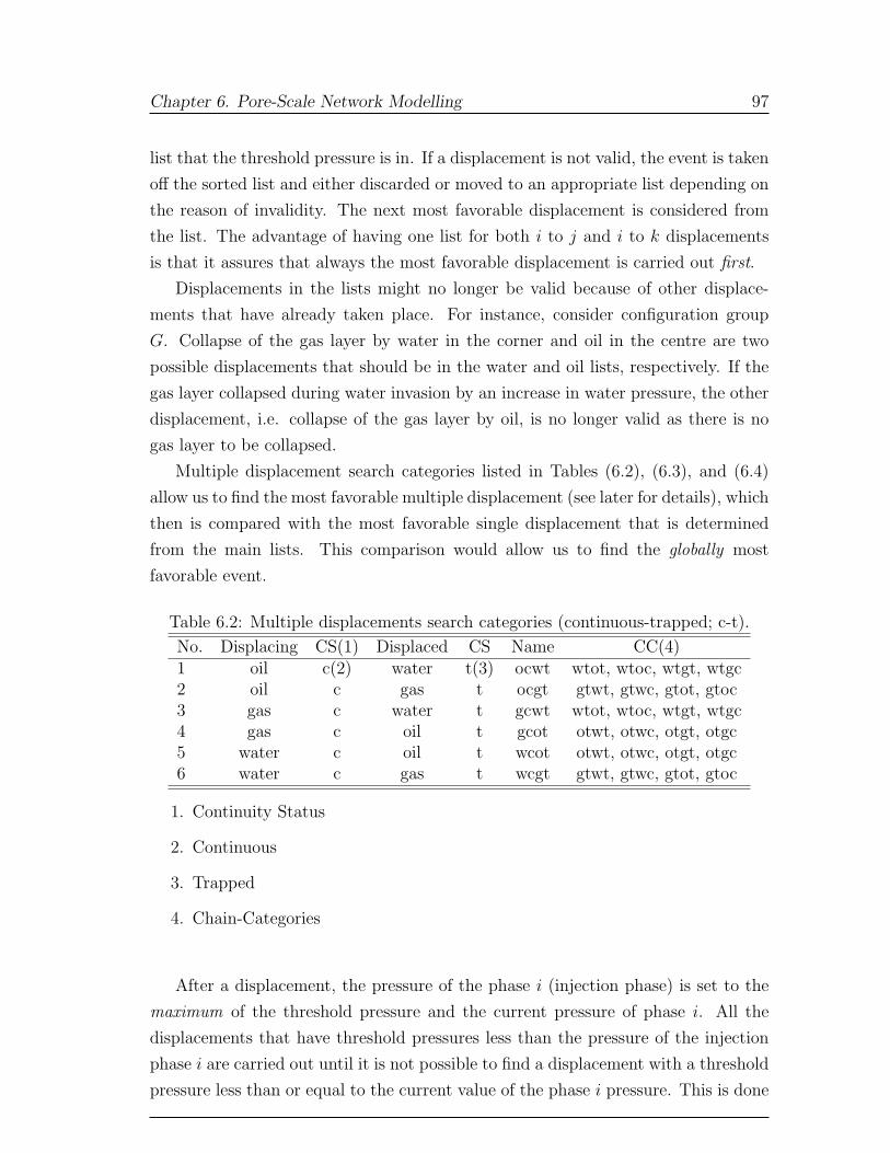
Chapter 6. Pore-Scale Network Modelling 97
list that the threshold pressure is in. If a displacement is not valid, the event is taken
off the sorted list and either discarded or moved to an appropriate list depending on
the reason of invalidity. The next most favorable displacement is considered from
the list. The advantage of having one list for both i to j and i to k displacements
is that it assures that always the most favorable displacement is carried out first.
Displacements in the lists might no longer be valid because of other displace-
ments that have already taken place. For instance, consider configuration group
G. Collapse of the gas layer by water in the corner and oil in the centre are two
possible displacements that should be in the water and oil lists, respectively. If the
gas layer collapsed during water invasion by an increase in water pressure, the other
displacement, i.e. collapse of the gas layer by oil, is no longer valid as there is no
gas layer to be collapsed.
Multiple displacement search categories listed in Tables (6.2), (6.3), and (6.4)
allow us to find the most favorable multiple displacement (see later for details), which
then is compared with the most favorable single displacement that is determined
from the main lists. This comparison would allow us to find the globally most
favorable event.
Table 6.2: Multiple displacements search categories (continuous-trapped; c-t).
No. Displacing CS(1) Displaced CS Name CC(4)1 oil c(2) water t(3) ocwt wtot, wtoc, wtgt, wtgc2 oil c gas t ocgt gtwt, gtwc, gtot, gtoc3 gas c water t gcwt wtot, wtoc, wtgt, wtgc4 gas c oil t gcot otwt, otwc, otgt, otgc5 water c oil t wcot otwt, otwc, otgt, otgc6 water c gas t wcgt gtwt, gtwc, gtot, gtoc
1. Continuity Status
2. Continuous
3. Trapped
4. Chain-Categories
After a displacement, the pressure of the phase i (injection phase) is set to the
maximum of the threshold pressure and the current pressure of phase i. All the
displacements that have threshold pressures less than the pressure of the injection
phase i are carried out until it is not possible to find a displacement with a threshold
pressure less than or equal to the current value of the phase i pressure. This is done
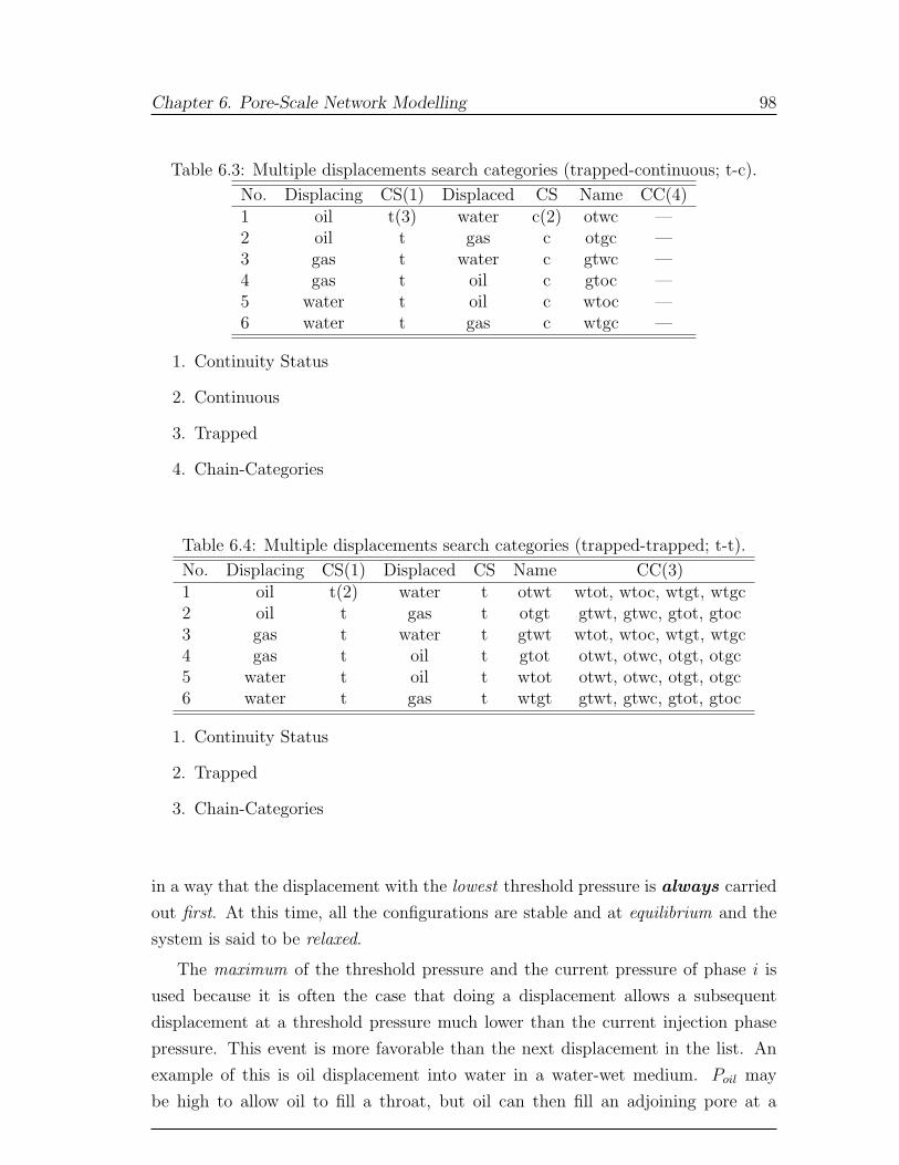
Chapter 6. Pore-Scale Network Modelling 98
Table 6.3: Multiple displacements search categories (trapped-continuous; t-c).
No. Displacing CS(1) Displaced CS Name CC(4)1 oil t(3) water c(2) otwc —2 oil t gas c otgc —3 gas t water c gtwc —4 gas t oil c gtoc —5 water t oil c wtoc —6 water t gas c wtgc —
1. Continuity Status
2. Continuous
3. Trapped
4. Chain-Categories
Table 6.4: Multiple displacements search categories (trapped-trapped; t-t).
No. Displacing CS(1) Displaced CS Name CC(3)1 oil t(2) water t otwt wtot, wtoc, wtgt, wtgc2 oil t gas t otgt gtwt, gtwc, gtot, gtoc3 gas t water t gtwt wtot, wtoc, wtgt, wtgc4 gas t oil t gtot otwt, otwc, otgt, otgc5 water t oil t wtot otwt, otwc, otgt, otgc6 water t gas t wtgt gtwt, gtwc, gtot, gtoc
1. Continuity Status
2. Trapped
3. Chain-Categories
in a way that the displacement with the lowest threshold pressure is always carried
out first. At this time, all the configurations are stable and at equilibrium and the
system is said to be relaxed.
The maximum of the threshold pressure and the current pressure of phase i is
used because it is often the case that doing a displacement allows a subsequent
displacement at a threshold pressure much lower than the current injection phase
pressure. This event is more favorable than the next displacement in the list. An
example of this is oil displacement into water in a water-wet medium. Poil may
be high to allow oil to fill a throat, but oil can then fill an adjoining pore at a
Chapter 6. Pore-Scale Network Modelling 99
lower oil pressure. If we used this new lower value of Poil to compute radii of
curvature, then we would find that in some elements the radius is inconsistent with
the fluid configuration – for instance, water AM in a corner would have a radius
of curvature too large to fit in an element. In strict capillary equilibrium, the fluid
would rearrange throughout the network to give configurations consistent with the
prevailing capillary pressure. This is, however, a very difficult task for a general
three-phase model. Instead, phase pressures are defined as the maximum value ever
reached during the whole simulation. In other words, the pressure of the invading
phase never acquires a lower value than its current one. Whenever a phase pressure
reaches a new maximum, the fluid configurations are truly in a position of capillary
equilibrium. In a simulation involving a complex displacement path, the phase
pressures will continue to increase. However, since it is only pressure differences
that control the displacement sequence, this is not a problem.
As mentioned earlier, threshold capillary pressures may be affected by the change
in capillary pressure. In such circumstances, threshold capillary pressures for those
displacements are recomputed taking into account the new arrangements of fluid and
capillary pressures and re-ordered in the sorted lists. The new phase saturations and
relative permeabilities are computed (see sections (6.5) and (6.6)) when the system
is relaxed. If a new phase is injected then the sorted lists for displacements are
re-ordered to account for latest changes in capillary pressures.
6.3 How to Treat the Trapped Clusters, Associ-
ated Radii of Curvatures and Displacements
Trapped phases will be in the form of clusters of phase locations. When a cluster of
phase locations becomes trapped, (1): A number is assigned to it. (2): The phase
of the cluster is stored. (3): Addresses of all the phase locations belonging to it
are stored. (4): Two flags are assigned to every single phase location indicating
that they are trapped and the the cluster number that they belong to. (5): All
the current capillary pressures, i.e. phase pressures, are stored. (6): The volume of
the trapped cluster, which is the summation of volume of its phase locations, when
it is trapped is stored as the original volume of the cluster. The original volume
is used in saturation calculations to account for volume errors caused by multiple
displacements (see section (6.5)). (7): If any of the phase locations of the cluster is
involved in a displacement then it is moved to an appropriate sublist in one of the
multiple displacement search categories. This could be a move from the main sorted

Chapter 6. Pore-Scale Network Modelling 100
lists to the categories listed in Tables (6.2) and (6.3). If any of the phase locations is
involved in displacements that are already in the search categories listed in Tables
(6.2) and (6.3), then they need to be moved into corresponding categories in Table
(6.4).
Every multiple displacement search category may contain several sorted sublists.
Every sorted sublist within the categories named in Tables (6.2) and (6.3) has a
cluster number associated with it and contains the threshold pressure of the valid
displacements where a trapped cluster can displace continuous fluid or vice versa.
Categories listed in Table (6.2) contain displacements where the displaced phase
location is trapped while the categories named in Table (6.3) have the opposite
situation. All the sublists are always sorted in ascending order. One should note
that the sublists within each category are completely independent from each other.
During different three-phase processes, there may be cases where a trapped clus-
ter touches one, two or several other trapped clusters with different phases. WAG
flooding with several injection cycles is an example of such a case. The touch-
ing points represent displacements whose threshold pressures are stored in sublists
within categories tabulated in Table (6.4). For every displacement both displacing
and displaced phase locations are trapped. One trapped cluster might be involved
in several sublists as every sublist represents the touching points between only two
trapped clusters with different fluids. For every sublist displacing and displaced
cluster, numbers are also stored.
When a trapped cluster forms, the curvature of all interfaces associated with
it need to be kept fixed as long as the cluster is trapped and it has not become
involved in multiple displacements. The conventional method in previously devel-
oped network models was that the interfaces were considered frozen. This was done
regardless of the pressure of the phase inside the trapped cluster and pressures of
the surrounding fluids. In this work, the pressure of the fluid inside the cluster is
not a dummy value. It has a physical meaning during the modelling of different
processes. The initial pressure of the cluster is the pressure of the phase when it
was first trapped. However, the pressure of the cluster changes according to the
change in the pressure of the surrounding phases in order to maintain the curvature
of the interfaces at the same value as when the trapped cluster first formed. As an
example, imagine water flooding into oil in a water-wet system. Trapped clusters
of oil form at different stages of water injection, i.e. at different oil/water capillary
pressures. Once each trapped cluster forms, it gets the current pressure of oil, i.e.
Poil. But since Poil is fixed during water flooding, all the trapped clusters will have
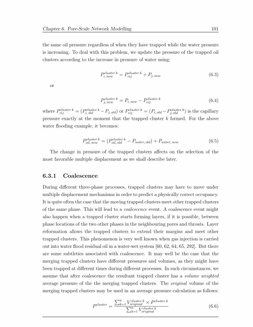
Chapter 6. Pore-Scale Network Modelling 101
the same oil pressure regardless of when they have trapped while the water pressure
is increasing. To deal with this problem, we update the pressure of the trapped oil
clusters according to the increase in pressure of water using:
P cluster ki, new = P cluster k
cij + Pj, new (6.3)
or
P cluster kj, new = Pi, new − P cluster k
cij (6.4)
where P cluster kcij = (P cluster k
i, old −Pj, old) or P cluster kcij = (Pi, old−P cluster k
j, old ) is the capillary
pressure exactly at the moment that the trapped cluster k formed. For the above
water flooding example, it becomes:
P cluster koil, new = (P cluster k
oil, old − Pwater, old) + Pwater, new (6.5)
The change in pressure of the trapped clusters affects on the selection of the
most favorable multiple displacement as we shall describe later.
6.3.1 Coalescence
During different three-phase processes, trapped clusters may have to move under
multiple displacement mechanisms in order to predict a physically correct occupancy.
It is quite often the case that the moving trapped clusters meet other trapped clusters
of the same phase. This will lead to a coalescence event. A coalescence event might
also happen when a trapped cluster starts forming layers, if it is possible, between
phase locations of the two other phases in the neighbouring pores and throats. Layer
reformation allows the trapped clusters to extend their margins and meet other
trapped clusters. This phenomenon is very well known when gas injection is carried
out into water flood residual oil in a water-wet system [60, 62, 64, 65, 292]. But there
are some subtleties associated with coalescence. It may well be the case that the
merging trapped clusters have different pressures and volumes, as they might have
been trapped at different times during different processes. In such circumstances, we
assume that after coalescence the resultant trapped cluster has a volume weighted
average pressure of the the merging trapped clusters. The original volume of the
merging trapped clusters may be used in an average pressure calculation as follows:
P cluster =
∑nk=1 V cluster k
original × P cluster k
∑nk=1 V cluster k
original
(6.6)
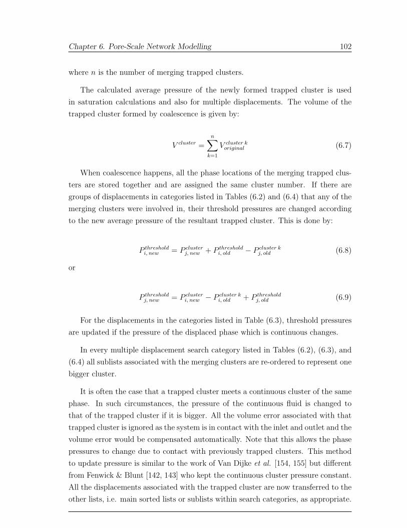
Chapter 6. Pore-Scale Network Modelling 102
where n is the number of merging trapped clusters.
The calculated average pressure of the newly formed trapped cluster is used
in saturation calculations and also for multiple displacements. The volume of the
trapped cluster formed by coalescence is given by:
V cluster =n∑
k=1
V cluster koriginal (6.7)
When coalescence happens, all the phase locations of the merging trapped clus-
ters are stored together and are assigned the same cluster number. If there are
groups of displacements in categories listed in Tables (6.2) and (6.4) that any of the
merging clusters were involved in, their threshold pressures are changed according
to the new average pressure of the resultant trapped cluster. This is done by:
P thresholdi, new = P cluster
j, new + P thresholdi, old − P cluster k
j, old (6.8)
or
P thresholdj, new = P cluster
i, new − P cluster ki, old + P threshold
j, old (6.9)
For the displacements in the categories listed in Table (6.3), threshold pressures
are updated if the pressure of the displaced phase which is continuous changes.
In every multiple displacement search category listed in Tables (6.2), (6.3), and
(6.4) all sublists associated with the merging clusters are re-ordered to represent one
bigger cluster.
It is often the case that a trapped cluster meets a continuous cluster of the same
phase. In such circumstances, the pressure of the continuous fluid is changed to
that of the trapped cluster if it is bigger. All the volume error associated with that
trapped cluster is ignored as the system is in contact with the inlet and outlet and the
volume error would be compensated automatically. Note that this allows the phase
pressures to change due to contact with previously trapped clusters. This method
to update pressure is similar to the work of Van Dijke et al. [154, 155] but different
from Fenwick & Blunt [142, 143] who kept the continuous cluster pressure constant.
All the displacements associated with the trapped cluster are now transferred to the
other lists, i.e. main sorted lists or sublists within search categories, as appropriate.
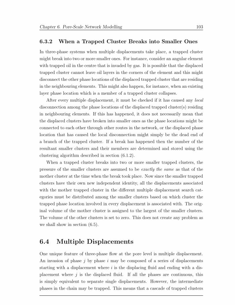
Chapter 6. Pore-Scale Network Modelling 103
6.3.2 When a Trapped Cluster Breaks into Smaller Ones
In three-phase systems when multiple displacements take place, a trapped cluster
might break into two or more smaller ones. For instance, consider an angular element
with trapped oil in the centre that is invaded by gas. It is possible that the displaced
trapped cluster cannot leave oil layers in the corners of the element and this might
disconnect the other phase locations of the displaced trapped cluster that are residing
in the neighbouring elements. This might also happen, for instance, when an existing
layer phase location which is a member of a trapped cluster collapses.
After every multiple displacement, it must be checked if it has caused any local
disconnection among the phase locations of the displaced trapped cluster(s) residing
in neighbouring elements. If this has happened, it does not necessarily mean that
the displaced clusters have broken into smaller ones as the phase locations might be
connected to each other through other routes in the network, or the displaced phase
location that has caused the local disconnection might simply be the dead end of
a branch of the trapped cluster. If a break has happened then the number of the
resultant smaller clusters and their members are determined and stored using the
clustering algorithm described in section (6.1.2).
When a trapped cluster breaks into two or more smaller trapped clusters, the
pressure of the smaller clusters are assumed to be exactly the same as that of the
mother cluster at the time when the break took place. Now since the smaller trapped
clusters have their own new independent identity, all the displacements associated
with the mother trapped cluster in the different multiple displacement search cat-
egories must be distributed among the smaller clusters based on which cluster the
trapped phase location involved in every displacement is associated with. The orig-
inal volume of the mother cluster is assigned to the largest of the smaller clusters.
The volume of the other clusters is set to zero. This does not create any problem as
we shall show in section (6.5).
6.4 Multiple Displacements
One unique feature of three-phase flow at the pore level is multiple displacement.
An invasion of phase j by phase i may be composed of a series of displacements
starting with a displacement where i is the displacing fluid and ending with a dis-
placement where j is the displaced fluid. If all the phases are continuous, this
is simply equivalent to separate single displacements. However, the intermediate
phases in the chain may be trapped. This means that a cascade of trapped clusters
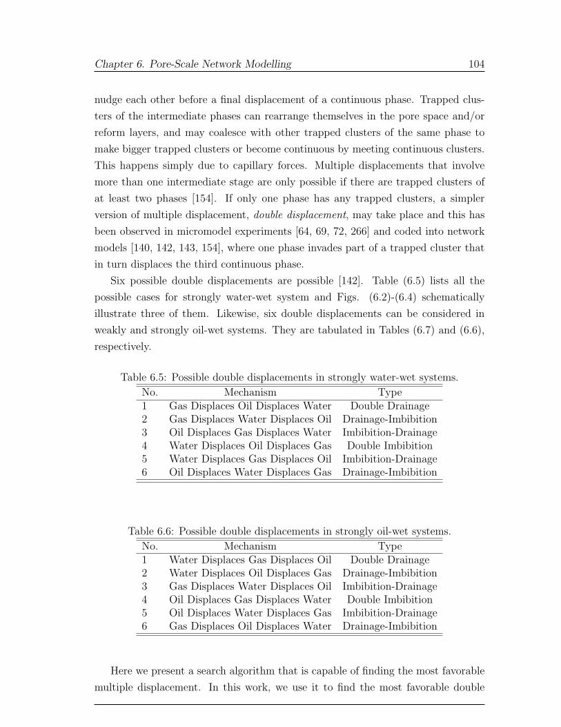
Chapter 6. Pore-Scale Network Modelling 104
nudge each other before a final displacement of a continuous phase. Trapped clus-
ters of the intermediate phases can rearrange themselves in the pore space and/or
reform layers, and may coalesce with other trapped clusters of the same phase to
make bigger trapped clusters or become continuous by meeting continuous clusters.
This happens simply due to capillary forces. Multiple displacements that involve
more than one intermediate stage are only possible if there are trapped clusters of
at least two phases [154]. If only one phase has any trapped clusters, a simpler
version of multiple displacement, double displacement, may take place and this has
been observed in micromodel experiments [64, 69, 72, 266] and coded into network
models [140, 142, 143, 154], where one phase invades part of a trapped cluster that
in turn displaces the third continuous phase.
Six possible double displacements are possible [142]. Table (6.5) lists all the
possible cases for strongly water-wet system and Figs. (6.2)-(6.4) schematically
illustrate three of them. Likewise, six double displacements can be considered in
weakly and strongly oil-wet systems. They are tabulated in Tables (6.7) and (6.6),
respectively.
Table 6.5: Possible double displacements in strongly water-wet systems.
No. Mechanism Type1 Gas Displaces Oil Displaces Water Double Drainage2 Gas Displaces Water Displaces Oil Drainage-Imbibition3 Oil Displaces Gas Displaces Water Imbibition-Drainage4 Water Displaces Oil Displaces Gas Double Imbibition5 Water Displaces Gas Displaces Oil Imbibition-Drainage6 Oil Displaces Water Displaces Gas Drainage-Imbibition
Table 6.6: Possible double displacements in strongly oil-wet systems.
No. Mechanism Type1 Water Displaces Gas Displaces Oil Double Drainage2 Water Displaces Oil Displaces Gas Drainage-Imbibition3 Gas Displaces Water Displaces Oil Imbibition-Drainage4 Oil Displaces Gas Displaces Water Double Imbibition5 Oil Displaces Water Displaces Gas Imbibition-Drainage6 Gas Displaces Oil Displaces Water Drainage-Imbibition
Here we present a search algorithm that is capable of finding the most favorable
multiple displacement. In this work, we use it to find the most favorable double
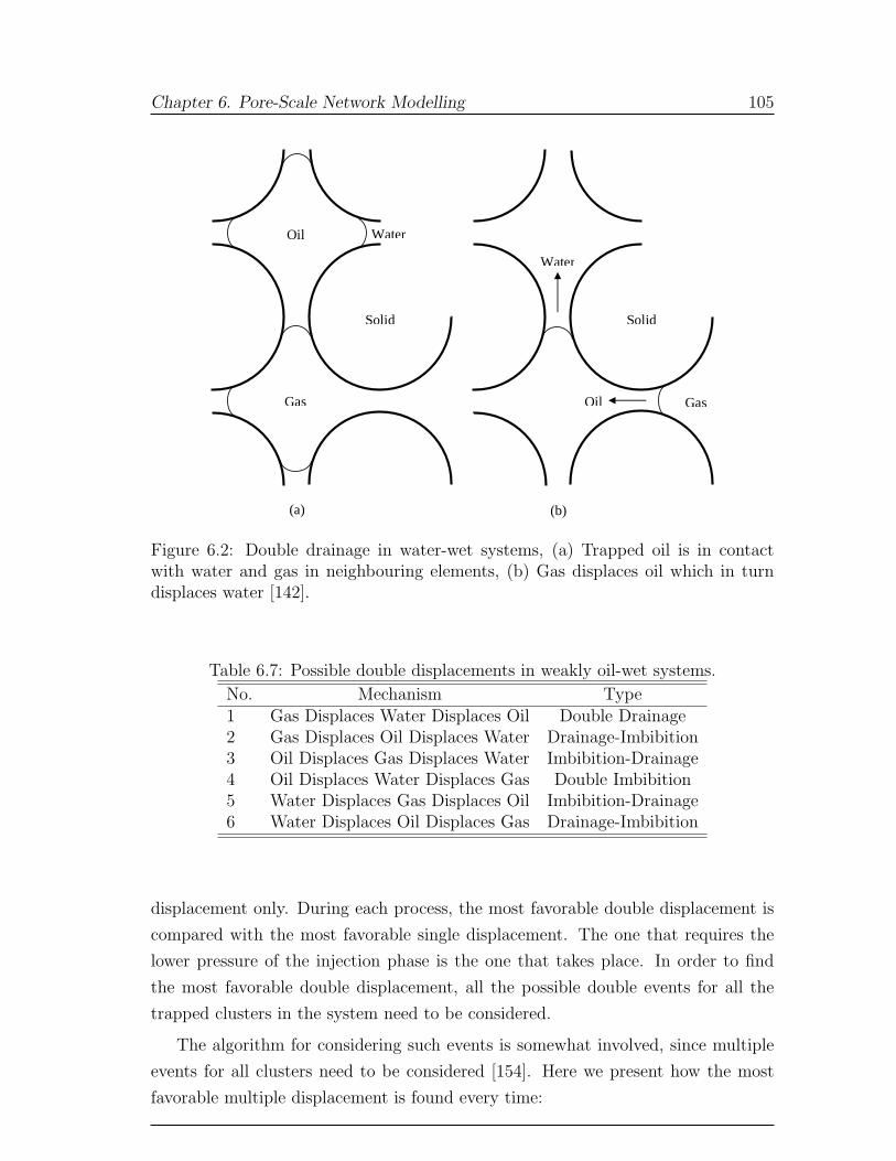
Chapter 6. Pore-Scale Network Modelling 105
Oil
Solid
Water
Gas
(a)
Gas
Water
Solid
Oil
(b)
Figure 6.2: Double drainage in water-wet systems, (a) Trapped oil is in contactwith water and gas in neighbouring elements, (b) Gas displaces oil which in turndisplaces water [142].
Table 6.7: Possible double displacements in weakly oil-wet systems.
No. Mechanism Type1 Gas Displaces Water Displaces Oil Double Drainage2 Gas Displaces Oil Displaces Water Drainage-Imbibition3 Oil Displaces Gas Displaces Water Imbibition-Drainage4 Oil Displaces Water Displaces Gas Double Imbibition5 Water Displaces Gas Displaces Oil Imbibition-Drainage6 Water Displaces Oil Displaces Gas Drainage-Imbibition
displacement only. During each process, the most favorable double displacement is
compared with the most favorable single displacement. The one that requires the
lower pressure of the injection phase is the one that takes place. In order to find
the most favorable double displacement, all the possible double events for all the
trapped clusters in the system need to be considered.
The algorithm for considering such events is somewhat involved, since multiple
events for all clusters need to be considered [154]. Here we present how the most
favorable multiple displacement is found every time:
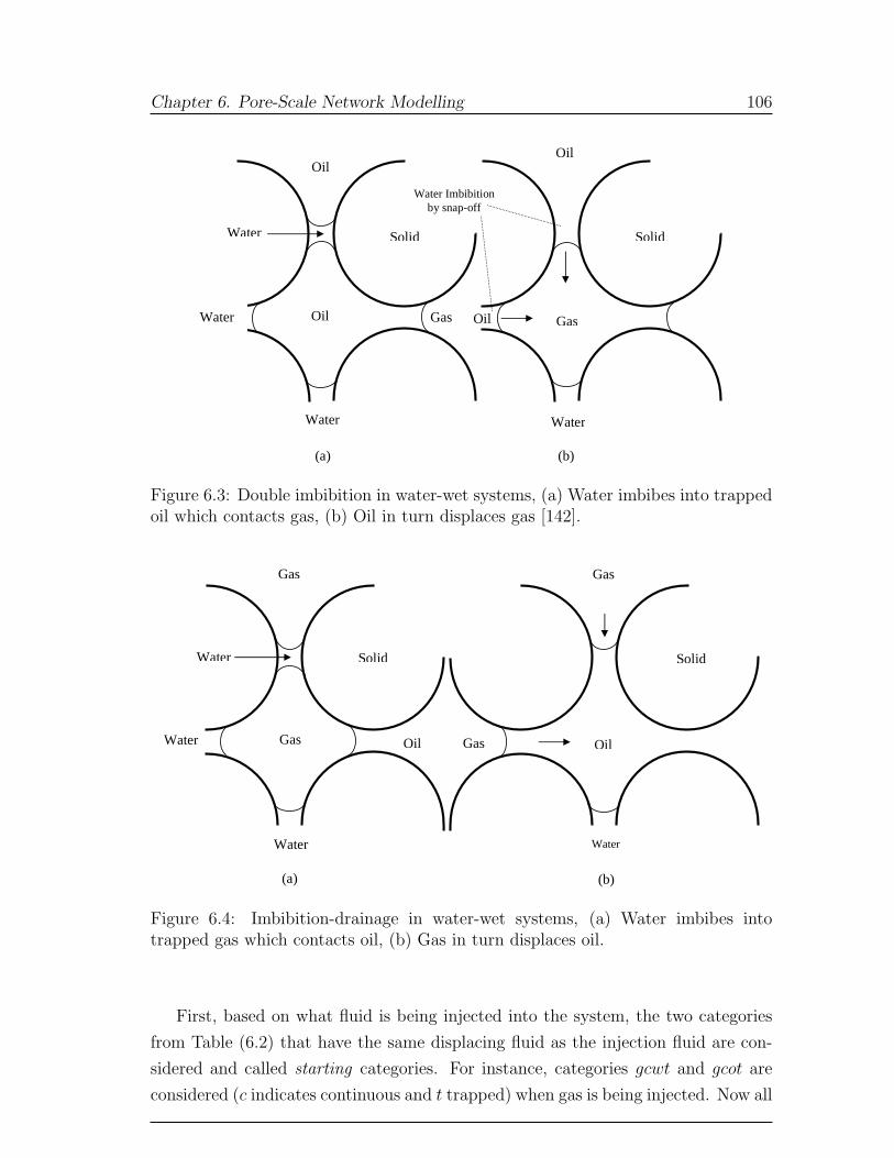
Chapter 6. Pore-Scale Network Modelling 106
Water Imbibition by snap-off
Oil
Solid
Water
Oil
Gas
(b)
Oil
Solid
Oil
Water
Water
Water
(a)
Gas
Figure 6.3: Double imbibition in water-wet systems, (a) Water imbibes into trappedoil which contacts gas, (b) Oil in turn displaces gas [142].
Oil
Solid
Gas
Water
Water Gas
Water
(a) (b)
Gas
Solid
Water
Oil
Gas
Figure 6.4: Imbibition-drainage in water-wet systems, (a) Water imbibes intotrapped gas which contacts oil, (b) Gas in turn displaces oil.
First, based on what fluid is being injected into the system, the two categories
from Table (6.2) that have the same displacing fluid as the injection fluid are con-
sidered and called starting categories. For instance, categories gcwt and gcot are
considered (c indicates continuous and t trapped) when gas is being injected. Now all

Chapter 6. Pore-Scale Network Modelling 107
the categories that could chain up with the starting categories are determined from
Tables (6.2), and (6.4) and are called chain-categories. Chain-categories for gcwt
and gcot would be wtot, wtoc, wtgt, wtgc, otwt, otwc, otgt, and otgc. As mentioned
earlier, every category might include several sublists with one or two trapped clus-
ter numbers associated with each one. The displacements at the top of each sublist
within the starting categories can now chain up with the displacements at the top of
the sublists within the chain-categories, if there are any, provided that the displacing
trapped cluster number of the sublist within the chain-category is the same as the
displaced trapped cluster number of the sublist within the starting category. This
means that every trapped cluster involved in a multiple displacement contributes to
two displacements. One should note that the displaced phase of a category must be
always the same as the displacing phase of the category that it is going to chain up
with. The displacement at the top of each sublist is the easiest, i.e. lowest invasion
pressure, displacement of the sublist. So every multiple displacement is a chain of
easiest displacements from sublists within categories that are allowed to chain up
with each other. Chaining up with categories continues until the next category is
one of those tabulated in Table (6.3). For example, the chain of gcot, otwt, wtgt
and gtwc could give multiple displacements provided that sublists satisfying the
foregoing conditions exist within the above categories. This in turn means that oil,
water, and gas trapped clusters existed in the system. Continuous gas is touching
trapped oil clusters which in turn touch trapped water clusters which in turn touch
trapped gas clusters which in turn touch continuous water. For a multiple displace-
ment with n trapped clusters involved, a series of n + 1 chainlike displacements are
carried out. Using the foregoing algorithm, all the possible multiple displacements
are determined and their threshold absolute pressure are calculated using:
P thresholdi, MD = P threshold
i +n∑
k=1
[(P thresholdj )cluster k − P cluster k
j, old ] (6.10)
where n is the number of trapped clusters involved, MD stands for multiple displace-
ment, P thresholdi is the threshold pressure of the first displacement of the multiple
displacement where the injection fluid is the displacing fluid, j is the fluid that
cluster k accommodates, (P thresholdj )cluster k is the threshold absolute pressure of the
displacement for which trapped cluster k is the displacing fluid, and P cluster kj, old is
the old pressure of the trapped cluster k, i.e. before the multiple displacement.
Eq. (6.10) has been derived by summing up the threshold capillary pressures of all
the displacements. One should note that the threshold capillary pressure of each
Chapter 6. Pore-Scale Network Modelling 108
displacement in a multiple displacement is calculated using a contact angle that is
defined according to what fluid is displacing what, regardless of what fluid is being
injected into the system. When a multiple displacement is carried out pressures of
the involved trapped clusters are increased to the value given by:
P cluster kj, new = (P threshold
j )cluster k (6.11)
We give an example of applying this algorithm by considering a double displace-
ment which is used in this work. Imagine gas is being injected into oil and water
where some of the oil is in trapped clusters. Since there are only trapped oil clusters
the only possible multiple displacement is double displacement where continuous
gas displaces trapped oil which in turn displaces continuous water. The double
displacements are determined by chaining up categories gcot and otwc provided
that the required sublists are present within each category. The threshold capillary
pressure of the double displacement is:
P thresholdgas, DD = P threshold
gas + [(P thresholdoil )cluster − P cluster
oil, old ] (6.12)
where DD stands for double displacement. The new pressure of the trapped oil
cluster is:
P clusteroil, new = (P threshold
oil )cluster (6.13)
Once a multiple displacement is recognized as a global most favorable event, it
is carried out. But there is one subtlety involved. It is quite often the case that
P thresholdi, MD is smaller than Pi. In other words, the multiple displacement could be
carried out without any increase in pressure of phase i. The difference between
these two pressures needs to be accounted for in the pressures of trapped clusters
involved in multiple displacement by increasing them by (Pi − P thresholdi, MD ).
When it comes to calculate the threshold pressure of a multiple displacement,
one may use threshold pressures of the displacements involved regardless of their
type. This means that displacements may well be layer formation or collapse events.
Theoretically this is fine but not technically. (I) This approach might increase the
volume error associated with multiple displacement as piston-like, pore-body filling
and snap-off events might chain up with the layer formation or collapse events which
would obviously be detrimental for volume-mass conservation. (II) The simulator
might be trapped in an infinite loop of forming and collapsing layers. To prevent
these problems, we shall use a slightly different approach where only threshold pres-
Chapter 6. Pore-Scale Network Modelling 109
sures of piston-like, pore-body filling and snap-off events are used in calculating
the threshold pressure of a multiple displacement. In this approach, when a multi-
ple displacement is to be carried out, all the layer formation or collapse events in
the involved sublists that are more favorable to the displacements used in P thresholdi, MD
calculations, are carried out first.
As we mentioned earlier, when a multiple displacement is taking place, pressures
of the involved trapped clusters increase. Once this happens, we then update all the
AM’s associated with the trapped clusters according to their new pressures. This
means that the volumes of the trapped clusters are always kept updated. Also the
new AM’s formed during the multiple displacements will have radii of curvatures
according to the new pressures of the trapped clusters that they belong to.
After every multiple displacement event, new displacements that are now avail-
able have to be added to the sublists within the correct categories. This means that
we might have new chains of displacements, i.e. multiple displacements, for the next
round. Also there might be phase locations that must be added to or omitted from
the involved trapped cluster(s). For example, imagine a trapped gas cluster is to
displace trapped oil in the centre of a triangular throat. Before the displacement,
configurations in all the corners are from group B and the centre phase location is
a member of a trapped oil cluster. Also imagine corner half angles, contact angles
and capillary pressures allow oil to reside as a layer in at least one corner after the
oil in the centre is displaced by gas. After the displacement, the configurations in
two corners are changed to C and in one corner to F . Once the configurations are
changed, the centre phase location must be omitted from the trapped oil cluster and
added to the trapped gas cluster as it now accommodates gas. Also one oil layer
phase location residing in one of the corners must be added to the displaced trapped
oil cluster. The new displacements that must be added to the appropriate lists are:
oil layer collapse by water in the corner to be added into the right sublist, i.e. the
sublist with the same cluster number, within the wcot category provided that water
in the corner is continuous, oil layer collapse by gas in the centre to be added into
the right sublist within the gtot category, snap-off of the gas in the centre by oil
layer to be added into the right sublist within the otgt category, snap-off of gas in
the centre by water in the corners to be added into the right sublist within the wcgt
category and other displacements in connection with continuous and trapped fluids
residing in the neighbouring elements.
Chapter 6. Pore-Scale Network Modelling 110
6.5 Saturation Computation
Saturation is computed when the phase pressure reaches a new maximum - this
means that the system is at equilibrium and it is not possible to carry out any
displacements with the current phase pressures. If V ip is the volume of phase p in
element i (including the water volume in clay) then the saturation of phase p is
given by:
Sp =
∑ne
i=1 V ip + V error
p∑np
j=1
∑ne
i=1 V ij +
∑np
j=1 V errorj
(6.14)
where np is the number of phases, ne is the total number of pores and throats, and
V errorp is the volume error of phase p caused by multiple displacements and is given
by:
V errorp =
ncp∑
i=1
(V originalp − V present
p )i (6.15)
where ncp is the number of trapped clusters of phase p. The total volume, inscribed
radius, and shape of each element are read in as input data. The volume of a phase
in an element is the total volume multiplied by the fraction of the cross-sectional
area occupied by that phase. One should note that saturation is computed within
the selected region, i.e. between inlet and outlet surfaces of the network rather than
over the whole network (see section (6.6) for details). Expressions used to compute
areas are given next.
6.5.1 Area Open to Flow
The equations used to compute the total area of a pore or throat with different
cross-sections are:
At = πR2 Circular cross− section (6.16)
At = 4R2 Square cross− section (6.17)
At =R2
4GTriangular cross− section (6.18)
where R and G are the inscribed radius and shape factor of the pore or throat,
respectively.
The corner area open to flow is calculated using:
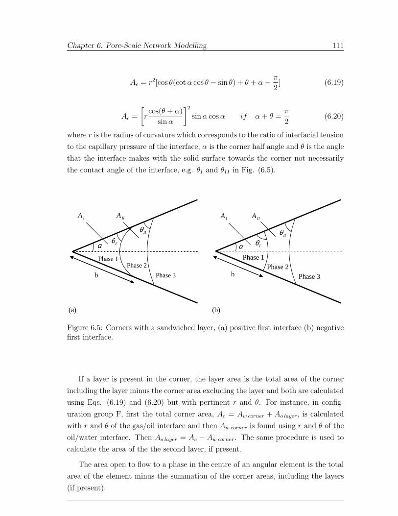
Chapter 6. Pore-Scale Network Modelling 111
Ac = r2[cos θ(cot α cos θ − sin θ) + θ + α− π
2] (6.19)
Ac =
[rcos(θ + α)
sin α
]2
sin α cos α if α + θ =π
2(6.20)
where r is the radius of curvature which corresponds to the ratio of interfacial tension
to the capillary pressure of the interface, α is the corner half angle and θ is the angle
that the interface makes with the solid surface towards the corner not necessarily
the contact angle of the interface, e.g. θI and θII in Fig. (6.5).
IA IIA
(b)
α
b
Phase 1 Phase 2
Phase 3
IIθ
Iθ
(a)
b
IIθ
α
Phase 1 Phase 2
Phase 3
IA IIA
Iθ
Figure 6.5: Corners with a sandwiched layer, (a) positive first interface (b) negativefirst interface.
If a layer is present in the corner, the layer area is the total area of the corner
including the layer minus the corner area excluding the layer and both are calculated
using Eqs. (6.19) and (6.20) but with pertinent r and θ. For instance, in config-
uration group F, first the total corner area, Ac = Aw corner + Ao layer, is calculated
with r and θ of the gas/oil interface and then Aw corner is found using r and θ of the
oil/water interface. Then Ao layer = Ac − Aw corner. The same procedure is used to
calculate the area of the the second layer, if present.
The area open to flow to a phase in the centre of an angular element is the total
area of the element minus the summation of the corner areas, including the layers
(if present).
Chapter 6. Pore-Scale Network Modelling 112
6.6 Conductances - Absolute and Relative Per-
meabilities
When saturation is computed, relative permeability and capillary pressure can also
be found. This is not done after every saturation computation to save computer
time. Typically, relative permeability is calculated around 20 - 40 times during a
simulation. To compute absolute and relative permeability, conductances of each
continuous phase location in each element are first computed. Normally exact an-
alytic results are not possible, and empirical expressions derived from solutions of
the Stoke’s equation for flow in pores of different geometries and for different fluid
configurations are used [76–78, 127, 264, 293, 294]. See later for expressions for the
conductances of each phase for the configurations shown in Figs. (5.1) and (5.2).
Then the average conductance for each phase in the whole network is computed by
explicitly calculating the flow through the network assuming conservation of volume.
From this absolute and relative permeability can be found [77, 127, 142, 290].
Solving the system of linear equations for each phase gives the pressure of that
phase in all the pores that contain that continuous phase. If there is an interface
between any of the phases in a pore or between the pore and connected throats then
the difference between the pressures of those two phases in that pore corresponds
to capillary pressure between those two phases [146].
In order to minimize end effects on calculated macroscopic properties, we cal-
culate the properties within two surfaces perpendicular to the main flow direction
bounding the central 90% of the network. However, the pressure is solved over
whole network to find the pressure in each pore. The pressure of the fluid whose
permeability is being calculated is found at the two surfaces by:
Pa =
∑ni=1 P i
a Aia∑n
i=1 Aia
(6.21)
where Pa is the pressure of phase a at the surface, P ia is the pressure of phase a in
a pore or throat at the point that touches the surface, Aia is the area open to flow
for phase a through that pore or throat, and n is the number of pores and throats
touching the surface. When the element that touches the surface is a pore then the
pressure of the phase a at the touching point will be the pore pressure of fluid a and
is known after the pressure is solved over the whole network. But if it is a throat,
then the pressure at the touching point is found by a linear interpolation between
the pressures of phase a in two connecting pores located in two sides of the surface.
Chapter 6. Pore-Scale Network Modelling 113
This is similar to the procedure used by Øren et al. [77].
The absolute permeability of the network is calculated using Darcy’s law:
K =µa Qtotal
a L
A∆P(6.22)
where K is the absolute permeability, µa the viscosity of fluid a, L is the distance
and ∆P is the corresponding pressure drop between the vertical surfaces. A is the
cross-sectional area perpendicular to the main direction of flow, Qtotala is the total
flow rate of fluid a.
First it is assumed that the network is completely filled with only one phase, e.g.
a. Conductance is calculated using the following equations [77, 281]:
g =0.5GA2
µCircular cross− section (6.23)
g =0.5623GA2
µSquare cross− section (6.24)
And for triangular cross-sections:
g =3R2A
20µ(6.25)
A pore might be connected to several other pores by throats (see Fig. (6.6)).
The conductance of a phase a, through an assembly of two pores connected to each
other by a throat, is considered to be the harmonic mean of the conductance to the
phase through the pores and the connecting throat [142]:
Lij
gaij
=Ltij
gatij
+Lpij
gapi
+Lpji
gapj
(6.26)
where Lij is the distance between the centres of two connected pores, gaij is the
conductance of the assembly to phase a, Ltij is the throat length, gatij
the throat
conductance to phase a, Lpijand Lpji
are the half length of the pores, and gapi
and
gapj
are conductance of the pores i and j to phase a, respectively, see Fig. (6.6).
The flow rate of the phase between two connected pores, i.e. qaij is then given by
[142]:
qaij =
gaij
Lij
(P api− P a
pj) (6.27)
where P api
and P apj
are the pressures of fluid a in pores i and j respectively.
Conserving volume for fluid a in each pore gives:
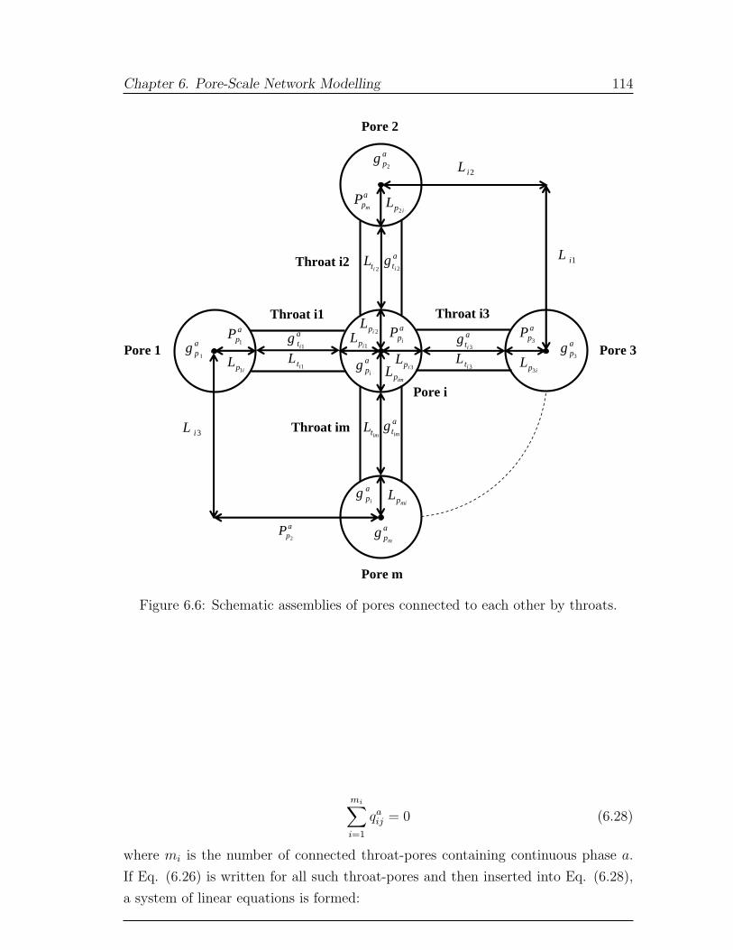
Chapter 6. Pore-Scale Network Modelling 114
Pore 3
Pore 2
apg
1
apg
2
apg
3
apm
g
Pore 1
Pore m
Throat i1 Throat i3
Throat i2
Throat im
ati
g3
ati
g2
ati
g1
1itL
imtL
2itL
3itL
atim
g
Pore i
ipL2
ipL3
mipL
ipL1
impL
3ipL
2ipL
1ipL api
P apP
3
apP
1
api
g
api
g
apm
P
apP
2
1iL
2iL
3iL
Figure 6.6: Schematic assemblies of pores connected to each other by throats.
mi∑i=1
qaij = 0 (6.28)
where mi is the number of connected throat-pores containing continuous phase a.
If Eq. (6.26) is written for all such throat-pores and then inserted into Eq. (6.28),
a system of linear equations is formed:
Chapter 6. Pore-Scale Network Modelling 115
P ap1
m1∑j=1
ga1j
L1j
−m1∑j=1
ga1j
L1j
P apj
= 0
P ap2
m2∑j=1
ga2j
L2j
−m2∑j=1
ga2j
L2j
P apj
= 0
...
P apn
mn∑j=1
ganj
Lnj
−mn∑j=1
ganj
Lnj
P apj
= 0 (6.29)
The resultant system of linear equations for the pore pressures is solved using the
Conjugate Gradient method [77]. Having the pore pressures allows us to calculate
the total flow rate of the phase, i.e. Qatotal, which in turn is used in Eq. (6.22) to
calculate the absolute permeability of the network, K.
Relative permeabilities are computed only when the network contains more than
one phase. They are calculated only for phases that have at least one network-
spanning cluster (a cluster that is continuous from inlet to outlet).
First the conductance in all the pore and throats containing continuous phase a
is computed. Then using the same procedure used for the calculation of absolute
permeability, the pressures of the phase in the pores that are a member of spanning
cluster(s) are found which in turn allows us to calculate relative permeability of the
phase by:
kar =
Qatotal
Qsingle phasetotal
(6.30)
Relative permeabilities are calculated only when the system is relaxed otherwise
there will be configurations that are not stable at the pressure at which the relative
permeabilities are calculated. The number of linear equations to be solved will be
lower than that for single-phase flow simply because the network is filled by multiple
phases meaning that not all the elements might contain continuous phase a.
When a network has elements with non-circular cross-section, a single element
might accommodate up to three fluids in it. A fluid, as it was shown in Figs. (5.1)
and (5.2), might be residing in corners, layers or the centre of a non-circular element.
For the fluid flowing through the centre of an element, Eqs. (6.23), (6.24), and (6.25)
are still used with A being only the area open to flow to the fluid at the centre.
Fluid flow through the corners and layers is yet more complex considering the

Chapter 6. Pore-Scale Network Modelling 116
involved physics. Parameters such as wettability, fluid-fluid and fluid-solid bound-
ary conditions, corner half angle, surface shear viscosity and physical properties of
fluids affect the conductances. This have been investigated by several authors. One
group has tried to solve the fluid flow numerically using Navier-Stokes equations and
then empirically correlate the numerical results and propose expressions for laminar
corner flow [77, 112, 293, 295–297]. Another approach is to apply the hydraulic
diameter approximation which was used by Lenormand and Zarcone [58] for flow
in square cross-section tubes. Blunt et al. [68] used a thin film flow approximation
to study the oil layer flow regime in a gravity drainage process. Later, Zhou et al.
[294] combined the hydraulic diameter and the thin film flow approximations to de-
rive expressions for corner and layer flow which were later modified by Hui & Blunt
[264, 265]. The proposed expressions were successful in predicting experimental
measurements [294, 298]. The authors found free and no-flow boundary conditions
suitable for gas/oil and oil/water interfaces, respectively.
In this work, we use the expressions proposed by Hui & Blunt [264, 265] to
compute the conductance of wetting and spreading layers.
When θI ≤ π2−α, see Fig. (6.5)-(a), the conductance of the element to the phase
flowing at the corner can be estimated by:
g =A2
c(1− sin α)2(ϕ2 cos θ − ϕ1)ϕ23
12µ sin2 α(1− ϕ3)2(ϕ2 + fϕ1)2(6.31)
ϕ1 = (π
2− α− θ) (6.32)
ϕ2 = cot α cos θ − sin θ (6.33)
ϕ3 = (π
2− α) tan α (6.34)
where θ = θI , Ac = AI , f = 1 for a no-flow boundary condition suitable for oil/water
interfaces, and f = 0 when a free boundary condition is applied for gas/oil or
gas/water interfaces.
If θI > π2− α, see Fig. (6.5)-(b), the corner conductance is calculated using:
g =A2
c tan α(1− sin α)2ϕ23
12µ sin2 α(1− ϕ3)(1 + fϕ3)2(6.35)
When there is a fluid layer sandwiched between the phases residing in the corner
and centre, corner and layer or layer and centre (see Figs. (5.1) and (5.2)), the
Chapter 6. Pore-Scale Network Modelling 117
conductance of the element to the sandwiched phase can be estimated by:
g =A3
1(1− sin α)2 tan αϕ23
12µAc sin2 α(1− ϕ3)[1 + f1ϕ3 − (1− f2ϕ3)
√A2
Ac
]2 (6.36)
where A1 is the area of the layer that the conductance is being calculated for, Ac
is a summation of areas of corner and layer (if present) above the layer of interest,
and A2 = Ac − A1. For instance, to calculate the conductance of the gas layer in
configuration group J, see Fig.(5.2), A1 = Ag layer, Ac = Aw corner +Ao layer +Ag layer,
and A2 = Aw corner + Ao layer. The corner and layer areas are calculated using Eqs.
(6.19) and (6.20).
6.7 Saturation Path Tracking
As several authors have shown (see section (3.1)), macroscopic properties in three-
phase systems are strongly dependent on the saturation history of the system. This
means that prediction of experimental measurements is possible only if the exper-
imental saturation history is reproduced by the model. It is only then that the
computed properties are comparable with their experimental counterparts. In this
work, we present an algorithm to track the experimental saturation paths on a point
by point basis.
Every given saturation path is composed of a series of points in saturation space.
The first saturation target (of oil, water, and gas) is specified. The difference be-
tween the present saturations and the target saturations are found. The phase with
the most negative difference is the next to be injected. Imagine this is phase i.
This means that we consider a displacement where the volume of i in an element
increases. Injection of phase i continues until the difference between the present and
the target saturation of phase i is not the most negative difference. Another phase
with the most negative difference is then injected. This continues until the satu-
ration differences fall within a predefined tolerance. Then a new saturation target
is considered. This process continues until the desired saturation path is produced,
see Fig. (6.7).
Tracking an experimental path using a network model is practically very complex
and difficult. This is because of finite size effects, the percolation nature of the
processes and hysteresis. For instance, in some cases during a saturation tracking
procedure, the system does not relax before several thousand displacements have
been performed which will take the saturations far away from the desired path.
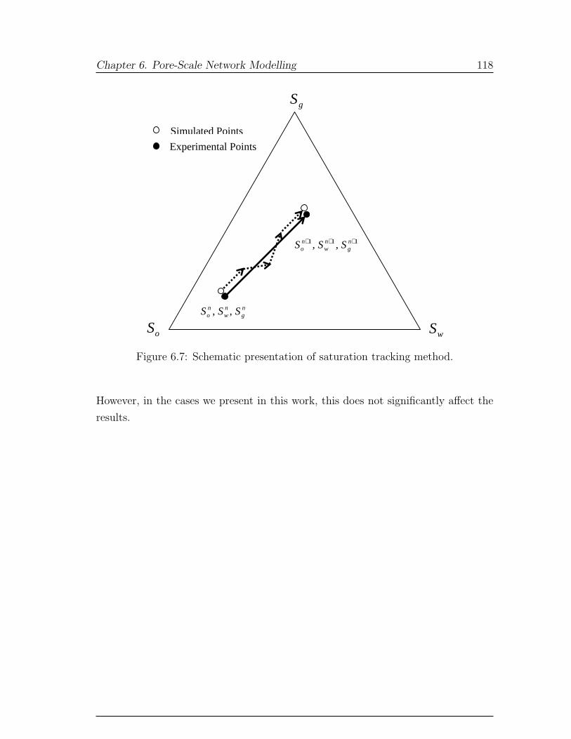
Chapter 6. Pore-Scale Network Modelling 118
ng
nw
no SSS ,,
111 ,, +++ ng
nw
no SSS
oS wS
gS
Simulated Points
Experimental Points
Figure 6.7: Schematic presentation of saturation tracking method.
However, in the cases we present in this work, this does not significantly affect the
results.
Chapter 7
Two- and Three-Phase Relative
Permeabilities
7.1 Comparison with Experiment
In this section, we use our model to simulate different two- and three-phase processes
at the pore-level and compare the results with their experimental counterparts.
The experiments we compare against will be two- and three-phase steady-state
measurements of relative permeability performed by Oak on water-wet Berea sand-
stone [1]. The fluids used by Oak were dodecane with 10% iodooctane, brine, and
air (nitrogen). Oak did not measure interfacial tensions. Pure dodecane/water/air
systems have a negative spreading coefficient; however it is known that the presence
of even small amounts of other alkanes in the oil can affect the spreading behaviour
significantly [245]. The low oil saturations reached in Oak’s experiments indicate a
spreading system as assumed by other authors who have studied this data [53, 149].
Consequently in this section we will use interfacial tensions for a spreading hex-
ane/water/air system – Table (7.1). These values are likely to be similar to those
in the experiments – small changes in the interfacial tensions, as long as the system
remains spreading, have a negligible impact on the results.
Oak studied three cores with permeabilities of 1000 mD, 800 mD, and 200 mD.
Our network has a permeability of 3055 mD (Table (4.2)). Oak found that the mea-
sured two-phase relative permeabilities for the least permeable core were different
from the other two. In our study we will only compare against data from the two
more permeable cores since their permeability and hence pore structure is likely to
be more representative of our network.
119
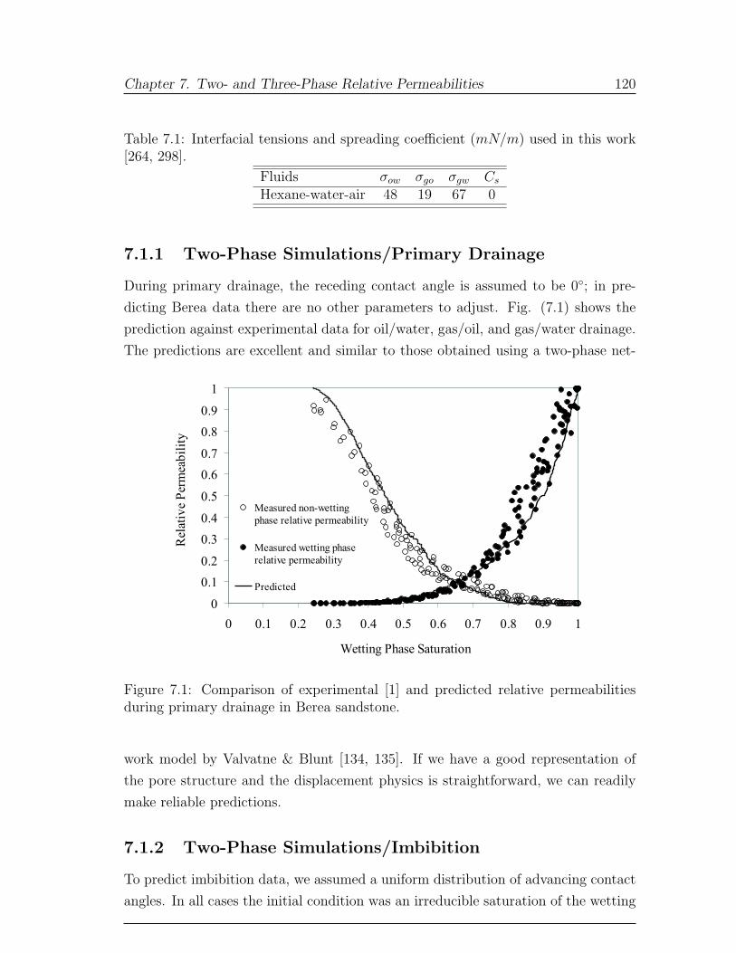
Chapter 7. Two- and Three-Phase Relative Permeabilities 120
Table 7.1: Interfacial tensions and spreading coefficient (mN/m) used in this work[264, 298].
Fluids σow σgo σgw Cs
Hexane-water-air 48 19 67 0
7.1.1 Two-Phase Simulations/Primary Drainage
During primary drainage, the receding contact angle is assumed to be 0◦; in pre-
dicting Berea data there are no other parameters to adjust. Fig. (7.1) shows the
prediction against experimental data for oil/water, gas/oil, and gas/water drainage.
The predictions are excellent and similar to those obtained using a two-phase net-
0
0.1
0.2
0.3
0.4
0.5
0.6
0.7
0.8
0.9
1
0 0.1 0.2 0.3 0.4 0.5 0.6 0.7 0.8 0.9 1
Wetting Phase Saturation
Rel
ativ
eP
erm
eab
ilit
y
Measured non-wetting
phase relative permeability
Measured wetting phase
relative permeability
Predicted
Figure 7.1: Comparison of experimental [1] and predicted relative permeabilitiesduring primary drainage in Berea sandstone.
work model by Valvatne & Blunt [134, 135]. If we have a good representation of
the pore structure and the displacement physics is straightforward, we can readily
make reliable predictions.
7.1.2 Two-Phase Simulations/Imbibition
To predict imbibition data, we assumed a uniform distribution of advancing contact
angles. In all cases the initial condition was an irreducible saturation of the wetting
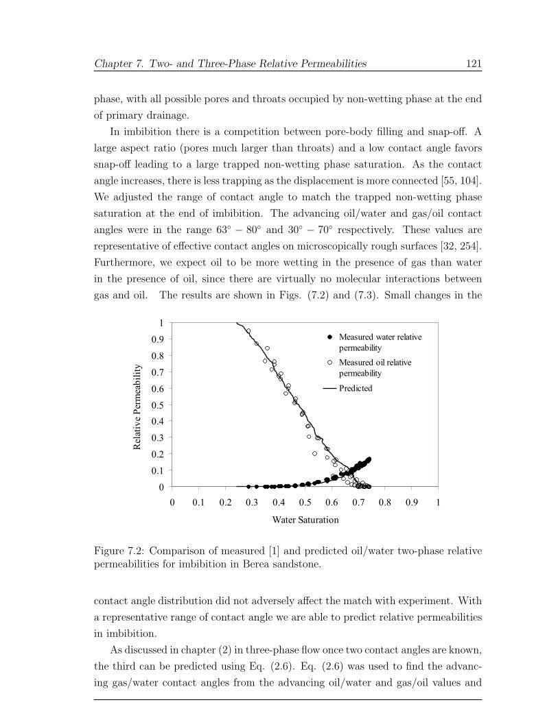
Chapter 7. Two- and Three-Phase Relative Permeabilities 121
phase, with all possible pores and throats occupied by non-wetting phase at the end
of primary drainage.
In imbibition there is a competition between pore-body filling and snap-off. A
large aspect ratio (pores much larger than throats) and a low contact angle favors
snap-off leading to a large trapped non-wetting phase saturation. As the contact
angle increases, there is less trapping as the displacement is more connected [55, 104].
We adjusted the range of contact angle to match the trapped non-wetting phase
saturation at the end of imbibition. The advancing oil/water and gas/oil contact
angles were in the range 63◦ − 80◦ and 30◦ − 70◦ respectively. These values are
representative of effective contact angles on microscopically rough surfaces [32, 254].
Furthermore, we expect oil to be more wetting in the presence of gas than water
in the presence of oil, since there are virtually no molecular interactions between
gas and oil. The results are shown in Figs. (7.2) and (7.3). Small changes in the
0
0.1
0.2
0.3
0.4
0.5
0.6
0.7
0.8
0.9
1
0 0.1 0.2 0.3 0.4 0.5 0.6 0.7 0.8 0.9 1
Water Saturation
Rel
ativ
eP
erm
eab
ilit
y
Measured water relative
permeability
Measured oil relative
permeability
Predicted
Figure 7.2: Comparison of measured [1] and predicted oil/water two-phase relativepermeabilities for imbibition in Berea sandstone.
contact angle distribution did not adversely affect the match with experiment. With
a representative range of contact angle we are able to predict relative permeabilities
in imbibition.
As discussed in chapter (2) in three-phase flow once two contact angles are known,
the third can be predicted using Eq. (2.6). Eq. (2.6) was used to find the advanc-
ing gas/water contact angles from the advancing oil/water and gas/oil values and
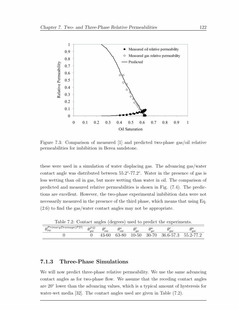
Chapter 7. Two- and Three-Phase Relative Permeabilities 122
0
0.1
0.2
0.3
0.4
0.5
0.6
0.7
0.8
0.9
1
0 0.1 0.2 0.3 0.4 0.5 0.6 0.7 0.8 0.9 1
Oil Saturation
Rel
ativ
eP
erm
eab
ilit
y
Measured oil relative permeability
Measured gas relative permeability
Predicted
Figure 7.3: Comparison of measured [1] and predicted two-phase gas/oil relativepermeabilities for imbibition in Berea sandstone.
these were used in a simulation of water displacing gas. The advancing gas/water
contact angle was distributed between 55.2◦-77.2◦. Water in the presence of gas is
less wetting than oil in gas, but more wetting than water in oil. The comparison of
predicted and measured relative permeabilities is shown in Fig. (7.4). The predic-
tions are excellent. However, the two-phase experimental imbibition data were not
necessarily measured in the presence of the third phase, which means that using Eq.
(2.6) to find the gas/water contact angles may not be appropriate.
Table 7.2: Contact angles (degrees) used to predict the experiments.
θPrimaryDrainage(PD)ow θPD
gw θrow θa
ow θrgo θa
go θrgw θa
gw
0 0 43-60 63-80 10-50 30-70 36.6-57.3 55.2-77.2
7.1.3 Three-Phase Simulations
We will now predict three-phase relative permeability. We use the same advancing
contact angles as for two-phase flow. We assume that the receding contact angles
are 20◦ lower than the advancing values, which is a typical amount of hysteresis for
water-wet media [32]. The contact angles used are given in Table (7.2).
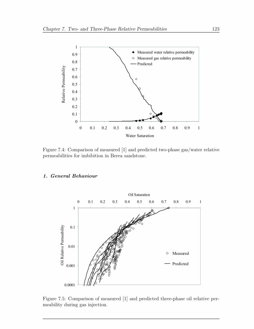
Chapter 7. Two- and Three-Phase Relative Permeabilities 123
0
0.1
0.2
0.3
0.4
0.5
0.6
0.7
0.8
0.9
1
0 0.1 0.2 0.3 0.4 0.5 0.6 0.7 0.8 0.9 1
Water Saturation
Rel
ativ
eP
erm
eabil
ity
Measured water relative permeability
Measured gas relative permeability
Predicted
Figure 7.4: Comparison of measured [1] and predicted two-phase gas/water relativepermeabilities for imbibition in Berea sandstone.
1. General Behaviour
0.0001
0.001
0.01
0.1
1
0 0.1 0.2 0.3 0.4 0.5 0.6 0.7 0.8 0.9 1
Oil Saturation
Oil
Rel
ativ
eP
erm
eab
ilit
y
Measured
Predicted
Figure 7.5: Comparison of measured [1] and predicted three-phase oil relative per-meability during gas injection.
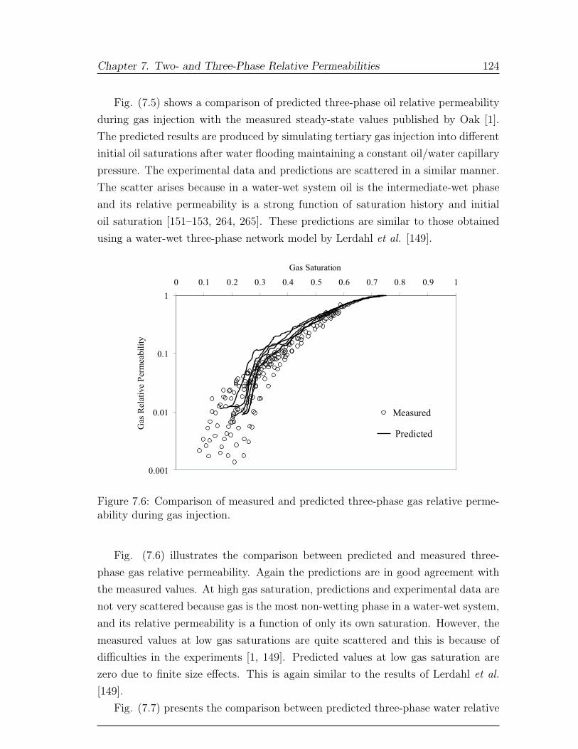
Chapter 7. Two- and Three-Phase Relative Permeabilities 124
Fig. (7.5) shows a comparison of predicted three-phase oil relative permeability
during gas injection with the measured steady-state values published by Oak [1].
The predicted results are produced by simulating tertiary gas injection into different
initial oil saturations after water flooding maintaining a constant oil/water capillary
pressure. The experimental data and predictions are scattered in a similar manner.
The scatter arises because in a water-wet system oil is the intermediate-wet phase
and its relative permeability is a strong function of saturation history and initial
oil saturation [151–153, 264, 265]. These predictions are similar to those obtained
using a water-wet three-phase network model by Lerdahl et al. [149].
0.001
0.01
0.1
1
0 0.1 0.2 0.3 0.4 0.5 0.6 0.7 0.8 0.9 1
Gas Saturation
Gas
Rel
ativ
eP
erm
eabil
ity
Measured
Predicted
Figure 7.6: Comparison of measured and predicted three-phase gas relative perme-ability during gas injection.
Fig. (7.6) illustrates the comparison between predicted and measured three-
phase gas relative permeability. Again the predictions are in good agreement with
the measured values. At high gas saturation, predictions and experimental data are
not very scattered because gas is the most non-wetting phase in a water-wet system,
and its relative permeability is a function of only its own saturation. However, the
measured values at low gas saturations are quite scattered and this is because of
difficulties in the experiments [1, 149]. Predicted values at low gas saturation are
zero due to finite size effects. This is again similar to the results of Lerdahl et al.
[149].
Fig. (7.7) presents the comparison between predicted three-phase water relative
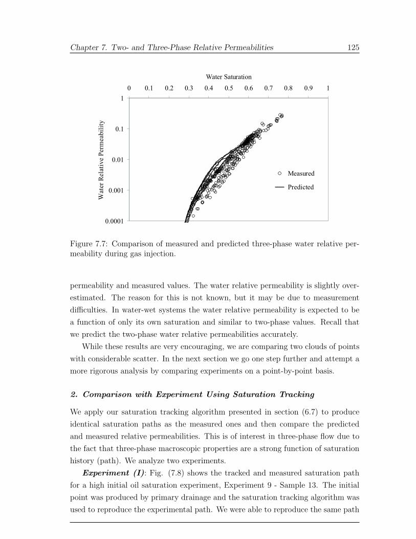
Chapter 7. Two- and Three-Phase Relative Permeabilities 125
0.0001
0.001
0.01
0.1
1
0 0.1 0.2 0.3 0.4 0.5 0.6 0.7 0.8 0.9 1
Water Saturation
Wat
erR
elat
ive
Per
mea
bil
ity
Measured
Predicted
Figure 7.7: Comparison of measured and predicted three-phase water relative per-meability during gas injection.
permeability and measured values. The water relative permeability is slightly over-
estimated. The reason for this is not known, but it may be due to measurement
difficulties. In water-wet systems the water relative permeability is expected to be
a function of only its own saturation and similar to two-phase values. Recall that
we predict the two-phase water relative permeabilities accurately.
While these results are very encouraging, we are comparing two clouds of points
with considerable scatter. In the next section we go one step further and attempt a
more rigorous analysis by comparing experiments on a point-by-point basis.
2. Comparison with Experiment Using Saturation Tracking
We apply our saturation tracking algorithm presented in section (6.7) to produce
identical saturation paths as the measured ones and then compare the predicted
and measured relative permeabilities. This is of interest in three-phase flow due to
the fact that three-phase macroscopic properties are a strong function of saturation
history (path). We analyze two experiments.
Experiment (I): Fig. (7.8) shows the tracked and measured saturation path
for a high initial oil saturation experiment, Experiment 9 - Sample 13. The initial
point was produced by primary drainage and the saturation tracking algorithm was
used to reproduce the experimental path. We were able to reproduce the same path
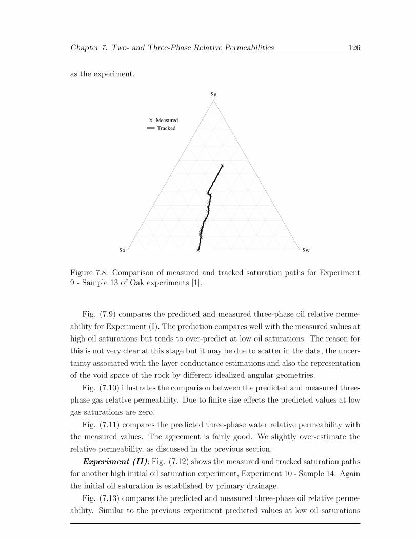
Chapter 7. Two- and Three-Phase Relative Permeabilities 126
as the experiment.
Measured
Tracked
So
Sg
Sw
Figure 7.8: Comparison of measured and tracked saturation paths for Experiment9 - Sample 13 of Oak experiments [1].
Fig. (7.9) compares the predicted and measured three-phase oil relative perme-
ability for Experiment (I). The prediction compares well with the measured values at
high oil saturations but tends to over-predict at low oil saturations. The reason for
this is not very clear at this stage but it may be due to scatter in the data, the uncer-
tainty associated with the layer conductance estimations and also the representation
of the void space of the rock by different idealized angular geometries.
Fig. (7.10) illustrates the comparison between the predicted and measured three-
phase gas relative permeability. Due to finite size effects the predicted values at low
gas saturations are zero.
Fig. (7.11) compares the predicted three-phase water relative permeability with
the measured values. The agreement is fairly good. We slightly over-estimate the
relative permeability, as discussed in the previous section.
Experiment (II): Fig. (7.12) shows the measured and tracked saturation paths
for another high initial oil saturation experiment, Experiment 10 - Sample 14. Again
the initial oil saturation is established by primary drainage.
Fig. (7.13) compares the predicted and measured three-phase oil relative perme-
ability. Similar to the previous experiment predicted values at low oil saturations
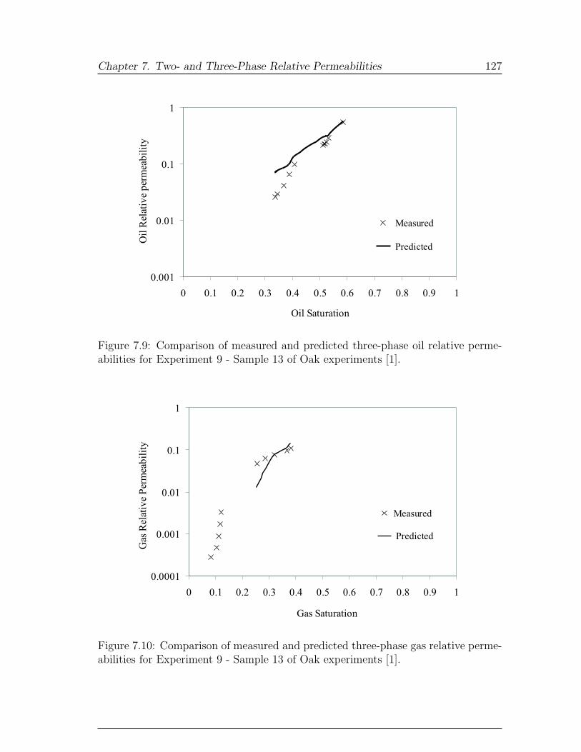
Chapter 7. Two- and Three-Phase Relative Permeabilities 127
0.001
0.01
0.1
1
0 0.1 0.2 0.3 0.4 0.5 0.6 0.7 0.8 0.9 1
Oil Saturation
Oil
Rel
ativ
ep
erm
eab
ilit
y
Measured
Predicted
Figure 7.9: Comparison of measured and predicted three-phase oil relative perme-abilities for Experiment 9 - Sample 13 of Oak experiments [1].
0.0001
0.001
0.01
0.1
1
0 0.1 0.2 0.3 0.4 0.5 0.6 0.7 0.8 0.9 1
Gas Saturation
Gas
Rel
ativ
eP
erm
eab
ilit
y
Measured
Predicted
Figure 7.10: Comparison of measured and predicted three-phase gas relative perme-abilities for Experiment 9 - Sample 13 of Oak experiments [1].
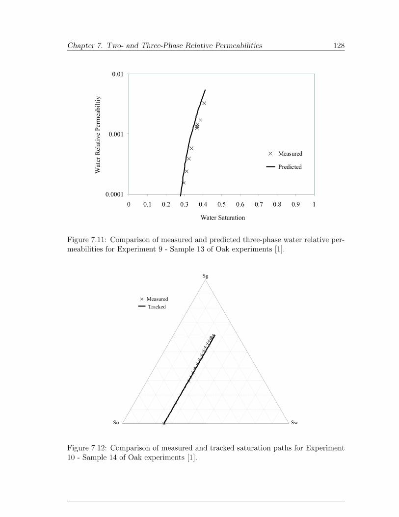
Chapter 7. Two- and Three-Phase Relative Permeabilities 128
0.0001
0.001
0.01
0 0.1 0.2 0.3 0.4 0.5 0.6 0.7 0.8 0.9 1
Water Saturation
Wat
erR
elat
ive
Per
mea
bil
tiy
Measured
Predicted
Figure 7.11: Comparison of measured and predicted three-phase water relative per-meabilities for Experiment 9 - Sample 13 of Oak experiments [1].
Measured
Tracked
So
Sg
Sw
Figure 7.12: Comparison of measured and tracked saturation paths for Experiment10 - Sample 14 of Oak experiments [1].
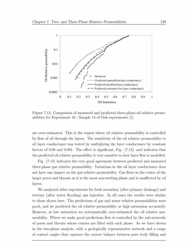
Chapter 7. Two- and Three-Phase Relative Permeabilities 129
0.0001
0.001
0.01
0.1
1
0 0.1 0.2 0.3 0.4 0.5 0.6 0.7 0.8 0.9 1
Oil Saturation
Oil
Rel
ativ
eper
mea
bil
ity
Measured
Predicted (unmodified layer conductance)
Predicted (modified layer conductance)
Predicted (extremely low layer conductance)
Figure 7.13: Comparison of measured and predicted three-phase oil relative perme-abilities for Experiment 10 - Sample 14 of Oak experiments [1].
are over-estimated. This is the region where oil relative permeability is controlled
by flow of oil through the layers. The sensitivity of the oil relative permeability to
oil layer conductance was tested by multiplying the layer conductance by constant
factors of 0.08 and 0.001. The effect is significant, Fig. (7.13), and indicates that
the predicted oil relative permeability is very sensitive to how layer flow is modelled.
Fig. (7.14) indicates the very good agreement between predicted and measured
three-phase gas relative permeability. Variations in the oil layer conductance does
not have any impact on the gas relative permeability. Gas flows in the centre of the
larger pores and throats as it is the most non-wetting phase and is unaffected by oil
layers.
We analyzed other experiments for both secondary (after primary drainage) and
tertiary (after water flooding) gas injection. In all cases the results were similar
to those shown here. The predictions of gas and water relative permeabilities were
good, and we predicted the oil relative permeability at high saturation accurately.
However, at low saturation we systematically over-estimated the oil relative per-
meability. Where we make good predictions flow is controlled by the sub-networks
of pores and throats whose centres are filled with each phase. As we have shown
in the two-phase analysis, with a geologically representative network and a range
of contact angles that captures the correct balance between pore body filling and
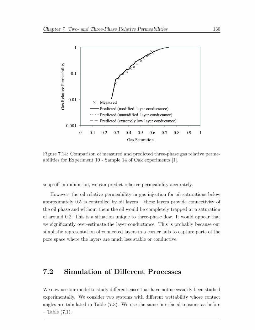
Chapter 7. Two- and Three-Phase Relative Permeabilities 130
0.001
0.01
0.1
1
0 0.1 0.2 0.3 0.4 0.5 0.6 0.7 0.8 0.9 1
Gas Saturation
Gas
Rel
ativ
eP
erm
eab
ilit
y
Measured
Predicted (modified layer conductance)
Predicted (unmodified layer conductance)
Predicted (extremely low layer conductance)
Figure 7.14: Comparison of measured and predicted three-phase gas relative perme-abilities for Experiment 10 - Sample 14 of Oak experiments [1].
snap-off in imbibition, we can predict relative permeability accurately.
However, the oil relative permeability in gas injection for oil saturations below
approximately 0.5 is controlled by oil layers – these layers provide connectivity of
the oil phase and without them the oil would be completely trapped at a saturation
of around 0.2. This is a situation unique to three-phase flow. It would appear that
we significantly over-estimate the layer conductance. This is probably because our
simplistic representation of connected layers in a corner fails to capture parts of the
pore space where the layers are much less stable or conductive.
7.2 Simulation of Different Processes
We now use our model to study different cases that have not necessarily been studied
experimentally. We consider two systems with different wettability whose contact
angles are tabulated in Table (7.3). We use the same interfacial tensions as before
– Table (7.1).
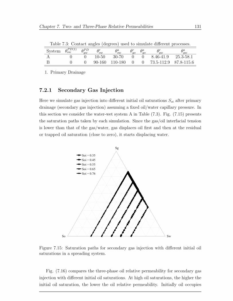
Chapter 7. Two- and Three-Phase Relative Permeabilities 131
Table 7.3: Contact angles (degrees) used to simulate different processes.
System θPD(1)ow θPD
gw θrow θa
ow θrgo θa
go θrgw θa
gw
A 0 0 10-50 30-70 0 0 8.46-41.9 25.3-58.1B 0 0 90-160 110-180 0 0 73.5-112.9 87.8-115.6
1. Primary Drainage
7.2.1 Secondary Gas Injection
Here we simulate gas injection into different initial oil saturations Soi after primary
drainage (secondary gas injection) assuming a fixed oil/water capillary pressure. In
this section we consider the water-wet system A in Table (7.3). Fig. (7.15) presents
the saturation paths taken by each simulation. Since the gas/oil interfacial tension
is lower than that of the gas/water, gas displaces oil first and then at the residual
or trapped oil saturation (close to zero), it starts displacing water.
Soi = 0.35
Soi = 0.45
Soi = 0.55
Soi = 0.65
Soi = 0.76
So Sw
Sg
Figure 7.15: Saturation paths for secondary gas injection with different initial oilsaturations in a spreading system.
Fig. (7.16) compares the three-phase oil relative permeability for secondary gas
injection with different initial oil saturations. At high oil saturations, the higher the
initial oil saturation, the lower the oil relative permeability. Initially oil occupies
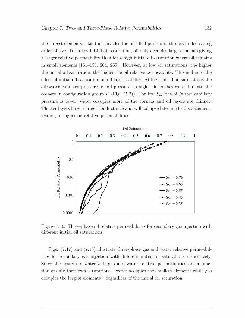
Chapter 7. Two- and Three-Phase Relative Permeabilities 132
the largest elements. Gas then invades the oil-filled pores and throats in decreasing
order of size. For a low initial oil saturation, oil only occupies large elements giving
a larger relative permeability than for a high initial oil saturation where oil remains
in small elements [151–153, 264, 265]. However, at low oil saturations, the higher
the initial oil saturation, the higher the oil relative permeability. This is due to the
effect of initial oil saturation on oil layer stability. At high initial oil saturations the
oil/water capillary pressure, or oil pressure, is high. Oil pushes water far into the
corners in configuration group F (Fig. (5.2)). For low Soi, the oil/water capillary
pressure is lower, water occupies more of the corners and oil layers are thinner.
Thicker layers have a larger conductance and will collapse later in the displacement,
leading to higher oil relative permeabilities.
0.0001
0.001
0.01
0.1
1
0 0.1 0.2 0.3 0.4 0.5 0.6 0.7 0.8 0.9 1
Oil Saturation
Oil
Rel
ativ
eP
erm
eabil
ity
Soi = 0.76
Soi = 0.65
Soi = 0.55
Soi = 0.45
Soi = 0.35
Figure 7.16: Three-phase oil relative permeabilities for secondary gas injection withdifferent initial oil saturations.
Figs. (7.17) and (7.18) illustrate three-phase gas and water relative permeabil-
ities for secondary gas injection with different initial oil saturations respectively.
Since the system is water-wet, gas and water relative permeabilities are a func-
tion of only their own saturations – water occupies the smallest elements while gas
occupies the largest elements – regardless of the initial oil saturation.
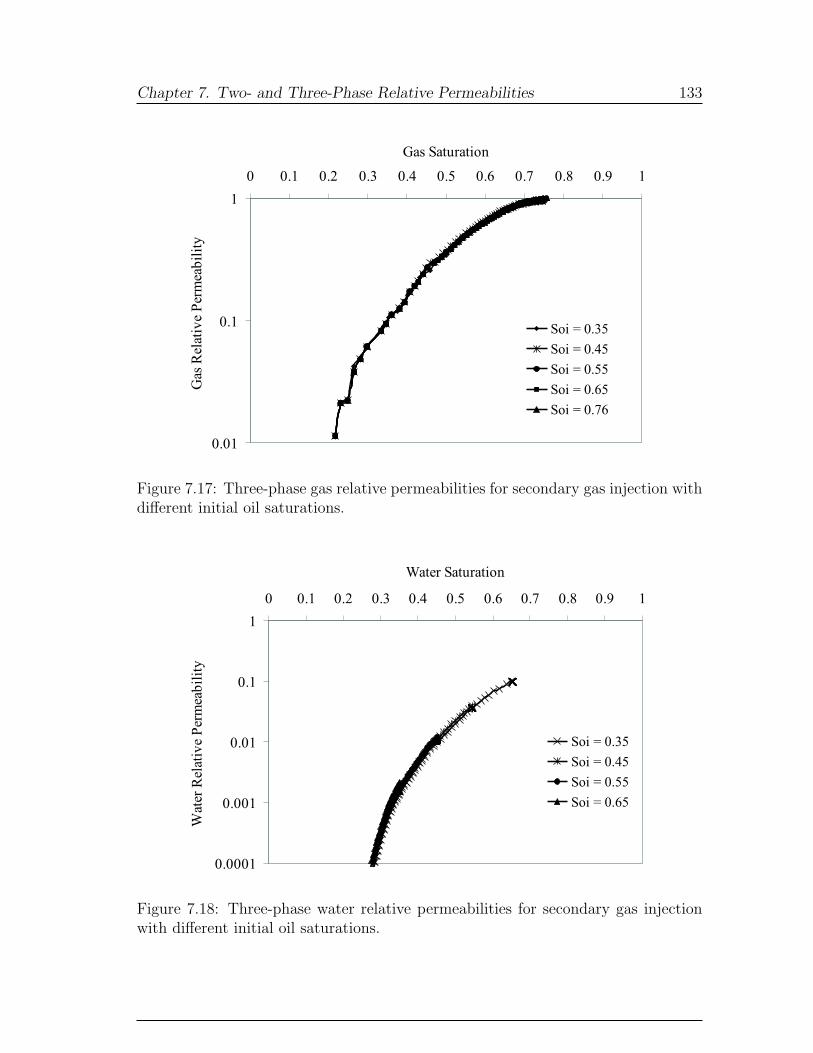
Chapter 7. Two- and Three-Phase Relative Permeabilities 133
0.01
0.1
1
0 0.1 0.2 0.3 0.4 0.5 0.6 0.7 0.8 0.9 1
Gas Saturation
Gas
Rel
ativ
eP
erm
eab
ilit
y
Soi = 0.35
Soi = 0.45
Soi = 0.55
Soi = 0.65
Soi = 0.76
Figure 7.17: Three-phase gas relative permeabilities for secondary gas injection withdifferent initial oil saturations.
0.0001
0.001
0.01
0.1
1
0 0.1 0.2 0.3 0.4 0.5 0.6 0.7 0.8 0.9 1
Water Saturation
Wat
erR
elat
ive
Per
mea
bil
ity
Soi = 0.35
Soi = 0.45
Soi = 0.55
Soi = 0.65
Figure 7.18: Three-phase water relative permeabilities for secondary gas injectionwith different initial oil saturations.
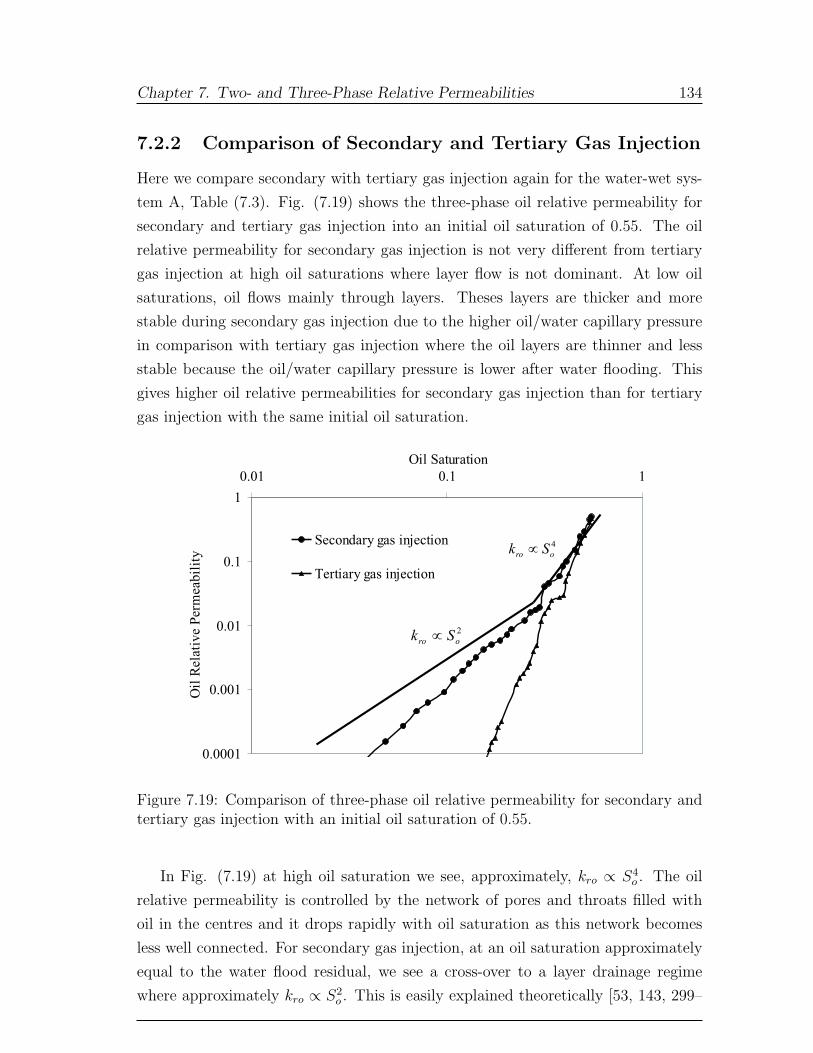
Chapter 7. Two- and Three-Phase Relative Permeabilities 134
7.2.2 Comparison of Secondary and Tertiary Gas Injection
Here we compare secondary with tertiary gas injection again for the water-wet sys-
tem A, Table (7.3). Fig. (7.19) shows the three-phase oil relative permeability for
secondary and tertiary gas injection into an initial oil saturation of 0.55. The oil
relative permeability for secondary gas injection is not very different from tertiary
gas injection at high oil saturations where layer flow is not dominant. At low oil
saturations, oil flows mainly through layers. Theses layers are thicker and more
stable during secondary gas injection due to the higher oil/water capillary pressure
in comparison with tertiary gas injection where the oil layers are thinner and less
stable because the oil/water capillary pressure is lower after water flooding. This
gives higher oil relative permeabilities for secondary gas injection than for tertiary
gas injection with the same initial oil saturation.
0.0001
0.001
0.01
0.1
1
0.01 0.1 1
Oil Saturation
Oil
Rel
ativ
eP
erm
eabil
ity
Secondary gas injection
Tertiary gas injection
4
oroSk µ
2
oroSk µ
Figure 7.19: Comparison of three-phase oil relative permeability for secondary andtertiary gas injection with an initial oil saturation of 0.55.
In Fig. (7.19) at high oil saturation we see, approximately, kro ∝ S4o . The oil
relative permeability is controlled by the network of pores and throats filled with
oil in the centres and it drops rapidly with oil saturation as this network becomes
less well connected. For secondary gas injection, at an oil saturation approximately
equal to the water flood residual, we see a cross-over to a layer drainage regime
where approximately kro ∝ S2o . This is easily explained theoretically [53, 143, 299–
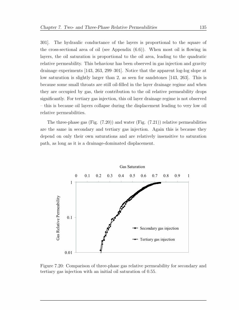
Chapter 7. Two- and Three-Phase Relative Permeabilities 135
301]. The hydraulic conductance of the layers is proportional to the square of
the cross-sectional area of oil (see Appendix (6.6)). When most oil is flowing in
layers, the oil saturation is proportional to the oil area, leading to the quadratic
relative permeability. This behaviour has been observed in gas injection and gravity
drainage experiments [143, 263, 299–301]. Notice that the apparent log-log slope at
low saturation is slightly larger than 2, as seen for sandstones [143, 263]. This is
because some small throats are still oil-filled in the layer drainage regime and when
they are occupied by gas, their contribution to the oil relative permeability drops
significantly. For tertiary gas injection, this oil layer drainage regime is not observed
– this is because oil layers collapse during the displacement leading to very low oil
relative permeabilities.
The three-phase gas (Fig. (7.20)) and water (Fig. (7.21)) relative permeabilities
are the same in secondary and tertiary gas injection. Again this is because they
depend on only their own saturations and are relatively insensitive to saturation
path, as long as it is a drainage-dominated displacement.
0.01
0.1
1
0 0.1 0.2 0.3 0.4 0.5 0.6 0.7 0.8 0.9 1
Gas Saturation
Gas
Rel
ativ
eP
erm
eab
ilit
y
Secondary gas injection
Tertiary gas injection
Figure 7.20: Comparison of three-phase gas relative permeability for secondary andtertiary gas injection with an initial oil saturation of 0.55.
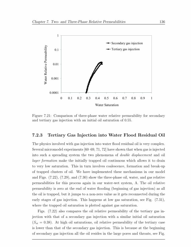
Chapter 7. Two- and Three-Phase Relative Permeabilities 136
0.0001
0.001
0.01
0.1
1
0 0.1 0.2 0.3 0.4 0.5 0.6 0.7 0.8 0.9 1
Water Saturation
Wat
erR
elat
ive
Per
mea
bil
ity
Secondary gas injection
Tertiary gas injection
Figure 7.21: Comparison of three-phase water relative permeability for secondaryand tertiary gas injection with an initial oil saturation of 0.55.
7.2.3 Tertiary Gas Injection into Water Flood Residual Oil
The physics involved with gas injection into water flood residual oil is very complex.
Several micromodel experiments [60–69, 71, 72] have shown that when gas is injected
into such a spreading system the two phenomena of double displacement and oil
layer formation make the initially trapped oil continuous which allows it to drain
to very low saturation. This in turn involves coalescence, formation and break-up
of trapped clusters of oil. We have implemented these mechanisms in our model
and Figs. (7.22), (7.29), and (7.30) show the three-phase oil, water, and gas relative
permeabilities for this process again in our water-wet system, A. The oil relative
permeability is zero at the end of water flooding (beginning of gas injection) as all
the oil is trapped, but it jumps to a non-zero value as it gets reconnected during the
early stages of gas injection. This happens at low gas saturation, see Fig. (7.31),
where the trapped oil saturation is plotted against gas saturation.
Figs. (7.22) also compares the oil relative permeability of the tertiary gas in-
jection with that of a secondary gas injection with a similar initial oil saturation
(Soi = 0.38). At high oil saturations, oil relative permeability of the tertiary case
is lower than that of the secondary gas injection. This is because at the beginning
of secondary gas injection all the oil resides in the large pores and throats, see Fig.

Chapter 7. Two- and Three-Phase Relative Permeabilities 137
0.0001
0.001
0.01
0.1
1
0 0.1 0.2 0.3 0.4 0.5 0.6 0.7 0.8 0.9 1
Oil Saturation
Oil
Rel
ativ
eP
erm
eab
ilit
yTertiary gas injection into
water flood residual oil
Secondary gas injection
Figure 7.22: Three-phase oil relative permeability for tertiary gas injection intowater flood residual oil (Soi = 0.384) and for secondary gas injection with a similarinitial oil saturation (Soi = 0.38).
(7.23), while at the beginning of the tertiary gas injection some of the oil stays in
the small elements due to trapping during water flooding, see Fig. (7.24). In other
words, the fraction of large oil filled elements at the starting point of secondary gas
injection is larger than that of tertiary case leading to lower oil relative permeabil-
ities for tertiary gas injection. However, at low oil saturations when the layer flow
is dominant, the oil relative permeability of the tertiary gas injection is higher since
during the displacement, double drainage causes an increase in oil/water capillary
pressure making oil layers thicker and more conductive.
Fig. (7.24) shows the pore and throat occupancy at the end of water flooding.
The trapped oil resides in the larger elements. During gas injection, double dis-
placement causes the oil to be pushed into smaller pores and throats while the gas
occupies the larger elements, see Figs. (7.25)-(7.28). The oil is now connected, since
it also resides in layers in gas-filled elements. This allows oil to be displaced and
results in a non-zero oil relative permeability, Fig. (7.22).
Fig. (7.29) shows the gas relative permeability compared to an equivalent sec-
ondary gas injection with (Soi = 0.38). The gas relative permeability for the tertiary
case is lower, in contrast to Fig. (7.20). The reason is that here the oil is trapped
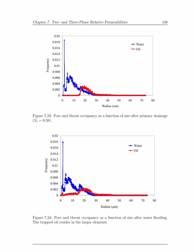
Chapter 7. Two- and Three-Phase Relative Permeabilities 138
0
0.002
0.004
0.006
0.008
0.01
0.012
0.014
0.016
0.018
0.02
0 10 20 30 40 50 60 70 80
Fre
quen
cyWater
Oil
Radius (µm)
Figure 7.23: Pore and throat occupancy as a function of size after primary drainage(So = 0.38).
0
0.002
0.004
0.006
0.008
0.01
0.012
0.014
0.016
0.018
0.02
0 10 20 30 40 50 60 70 80
Fre
quen
cy
Water
Oil
Radius (µm)
Figure 7.24: Pore and throat occupancy as a function of size after water flooding.The trapped oil resides in the larger elements.
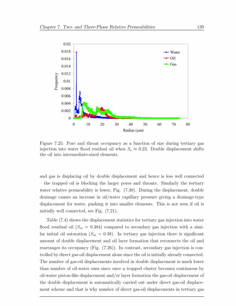
Chapter 7. Two- and Three-Phase Relative Permeabilities 139
0
0.002
0.004
0.006
0.008
0.01
0.012
0.014
0.016
0.018
0.02
0 10 20 30 40 50 60 70 80
Fre
quen
cyWater
Oil
Gas
Radius (µm)
Figure 7.25: Pore and throat occupancy as a function of size during tertiary gasinjection into water flood residual oil when So ≈ 0.23. Double displacement shiftsthe oil into intermediate-sized elements.
and gas is displacing oil by double displacement and hence is less well connected
– the trapped oil is blocking the larger pores and throats. Similarly the tertiary
water relative permeability is lower, Fig. (7.30). During the displacement, double
drainage causes an increase in oil/water capillary pressure giving a drainage-type
displacement for water, pushing it into smaller elements. This is not seen if oil is
initially well connected, see Fig. (7.21).
Table (7.4) shows the displacement statistics for tertiary gas injection into water
flood residual oil (Soi = 0.384) compared to secondary gas injection with a simi-
lar initial oil saturation (Soi = 0.38). In tertiary gas injection there is significant
amount of double displacement and oil layer formation that reconnects the oil and
rearranges its occupancy (Fig. (7.26)). In contrast, secondary gas injection is con-
trolled by direct gas-oil displacement alone since the oil is initially already connected.
The number of gas-oil displacements involved in double displacement is much lower
than number of oil-water ones since once a trapped cluster becomes continuous by
oil-water piston-like displacement and/or layer formation the gas-oil displacement of
the double displacement is automatically carried out under direct gas-oil displace-
ment scheme and that is why number of direct gas-oil displacements in tertiary gas
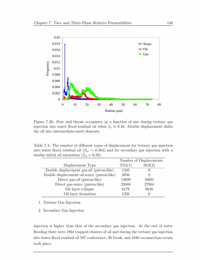
Chapter 7. Two- and Three-Phase Relative Permeabilities 140
0
0.002
0.004
0.006
0.008
0.01
0.012
0.014
0.016
0.018
0.02
0 10 20 30 40 50 60 70 80
Fre
quen
cyWater
Oil
Gas
Radius (µm)
Figure 7.26: Pore and throat occupancy as a function of size during tertiary gasinjection into water flood residual oil when So ≈ 0.16. Double displacement shiftsthe oil into intermediate-sized elements.
Table 7.4: The number of different types of displacement for tertiary gas injectioninto water flood residual oil (Soi = 0.384) and for secondary gas injection with asimilar initial oil saturation (Soi = 0.38).
Number of DisplacementsDisplacement Type TGI(1) SGI(2)
Double displacement gas-oil (piston-like) 1345 0Double displacement oil-water (piston-like) 3856 0
Direct gas-oil (piston-like) 13699 10091Direct gas-water (piston-like) 22688 27804
Oil layer collapse 6178 8640Oil layer formation 1356 0
1. Tertiary Gas Injection
2. Secondary Gas Injection
injection is higher than that of the secondary gas injection. At the end of water
flooding there were 1864 trapped clusters of oil and during the tertiary gas injection
into water flood residual oil 507 coalescence, 90 break, and 1040 reconnection events
took place.
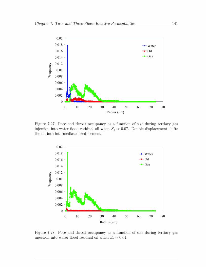
Chapter 7. Two- and Three-Phase Relative Permeabilities 141
0
0.002
0.004
0.006
0.008
0.01
0.012
0.014
0.016
0.018
0.02
0 10 20 30 40 50 60 70 80
Fre
quen
cyWater
Oil
Gas
Radius (µm)
Figure 7.27: Pore and throat occupancy as a function of size during tertiary gasinjection into water flood residual oil when So ≈ 0.07. Double displacement shiftsthe oil into intermediate-sized elements.
0
0.002
0.004
0.006
0.008
0.01
0.012
0.014
0.016
0.018
0.02
0 10 20 30 40 50 60 70 80
Fre
quen
cy
Water
Oil
Gas
Radius (µm)
Figure 7.28: Pore and throat occupancy as a function of size during tertiary gasinjection into water flood residual oil when So ≈ 0.01.
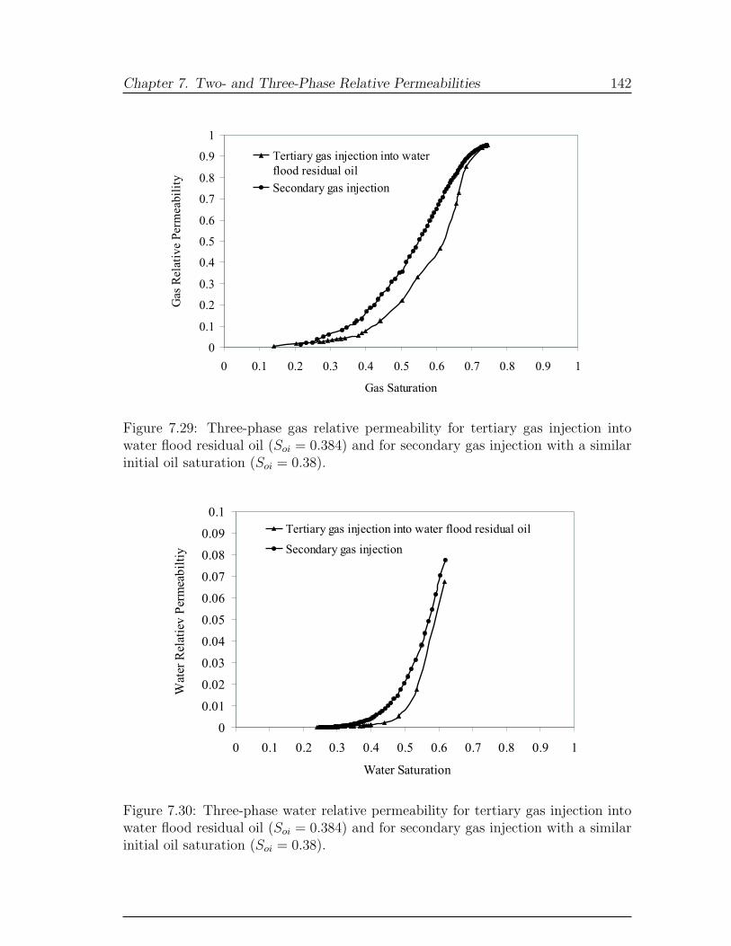
Chapter 7. Two- and Three-Phase Relative Permeabilities 142
0
0.1
0.2
0.3
0.4
0.5
0.6
0.7
0.8
0.9
1
0 0.1 0.2 0.3 0.4 0.5 0.6 0.7 0.8 0.9 1
Gas Saturation
Gas
Rel
ativ
eP
erm
eabil
ity
Tertiary gas injection into water
flood residual oil
Secondary gas injection
Figure 7.29: Three-phase gas relative permeability for tertiary gas injection intowater flood residual oil (Soi = 0.384) and for secondary gas injection with a similarinitial oil saturation (Soi = 0.38).
0
0.01
0.02
0.03
0.04
0.05
0.06
0.07
0.08
0.09
0.1
0 0.1 0.2 0.3 0.4 0.5 0.6 0.7 0.8 0.9 1
Water Saturation
Wat
erR
elat
iev
Per
mea
bil
tiy
Tertiary gas injection into water flood residual oil
Secondary gas injection
Figure 7.30: Three-phase water relative permeability for tertiary gas injection intowater flood residual oil (Soi = 0.384) and for secondary gas injection with a similarinitial oil saturation (Soi = 0.38).
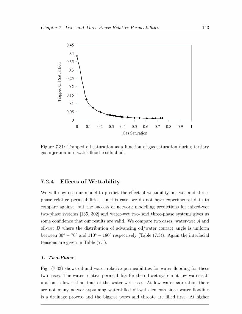
Chapter 7. Two- and Three-Phase Relative Permeabilities 143
0
0.05
0.1
0.15
0.2
0.25
0.3
0.35
0.4
0.45
0 0.1 0.2 0.3 0.4 0.5 0.6 0.7 0.8 0.9 1
Gas Saturation
Tra
pped
Oil
Sat
uar
tion
Figure 7.31: Trapped oil saturation as a function of gas saturation during tertiarygas injection into water flood residual oil.
7.2.4 Effects of Wettability
We will now use our model to predict the effect of wettability on two- and three-
phase relative permeabilities. In this case, we do not have experimental data to
compare against, but the success of network modelling predictions for mixed-wet
two-phase systems [135, 302] and water-wet two- and three-phase systems gives us
some confidence that our results are valid. We compare two cases: water-wet A and
oil-wet B where the distribution of advancing oil/water contact angle is uniform
between 30◦ − 70◦ and 110◦ − 180◦ respectively (Table (7.3)). Again the interfacial
tensions are given in Table (7.1).
1. Two-Phase
Fig. (7.32) shows oil and water relative permeabilities for water flooding for these
two cases. The water relative permeability for the oil-wet system at low water sat-
uration is lower than that of the water-wet case. At low water saturation there
are not many network-spanning water-filled oil-wet elements since water flooding
is a drainage process and the biggest pores and throats are filled first. At higher

Chapter 7. Two- and Three-Phase Relative Permeabilities 144
water saturation once water-filled elements span the system, the water relative per-
meability in the oil-wet system is larger since water occupies the larger pore spaces.
When the wettability changes from water-wet to oil-wet, the oil relative permeability
decreases since oil becomes the wetting phase and occupies the smaller pores and
throats.
0.001
0.01
0.1
1
0 0.1 0.2 0.3 0.4 0.5 0.6 0.7 0.8 0.9 1
Water Saturation
Rel
ativ
eP
erm
eabil
ity
Water-wet
Oil-wet
Figure 7.32: Oil and water relative permeability of water flooding in: (I) water-wet,θa
ow = 30◦ − 70◦ (system A), and (II) oil-wet, θaow = 110◦ − 180◦ (system B) Berea
sandstone.
The water-wet system has the higher residual oil saturation, 0.384, because snap-
off traps oil. A lower residual oil saturation, 0.0055, is found in the oil-wet system
since oil layers prevent trapping. This behaviour is consistent with that found by
other authors [113, 119, 120, 122, 303, 304]. Fig. (7.33) shows the pore and throat
occupancy as a function of size after water flooding in the oil-wet system, B.
2. Three-Phase
We consider primary drainage to irreducible water saturation followed by water
flooding to Sw = 0.4 (Soi = 0.6). Then gas is injected at a constant oil/water
capillary pressure.
Fig. (7.34) shows the oil relative permeability. In the oil-wet case, oil remains
in smaller pores and throats after water flooding than for a water-wet medium,
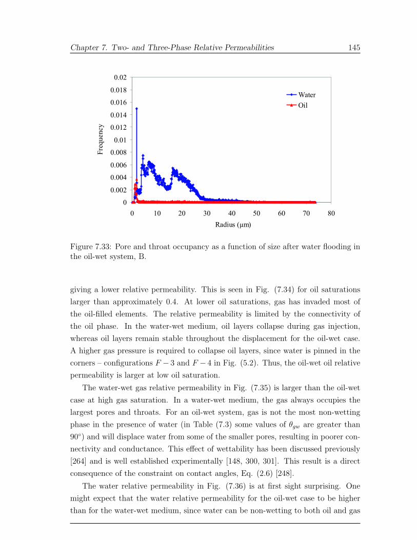
Chapter 7. Two- and Three-Phase Relative Permeabilities 145
0
0.002
0.004
0.006
0.008
0.01
0.012
0.014
0.016
0.018
0.02
0 10 20 30 40 50 60 70 80
Fre
quen
cyWater
Oil
Radius (µm)
Figure 7.33: Pore and throat occupancy as a function of size after water flooding inthe oil-wet system, B.
giving a lower relative permeability. This is seen in Fig. (7.34) for oil saturations
larger than approximately 0.4. At lower oil saturations, gas has invaded most of
the oil-filled elements. The relative permeability is limited by the connectivity of
the oil phase. In the water-wet medium, oil layers collapse during gas injection,
whereas oil layers remain stable throughout the displacement for the oil-wet case.
A higher gas pressure is required to collapse oil layers, since water is pinned in the
corners – configurations F − 3 and F − 4 in Fig. (5.2). Thus, the oil-wet oil relative
permeability is larger at low oil saturation.
The water-wet gas relative permeability in Fig. (7.35) is larger than the oil-wet
case at high gas saturation. In a water-wet medium, the gas always occupies the
largest pores and throats. For an oil-wet system, gas is not the most non-wetting
phase in the presence of water (in Table (7.3) some values of θgw are greater than
90◦) and will displace water from some of the smaller pores, resulting in poorer con-
nectivity and conductance. This effect of wettability has been discussed previously
[264] and is well established experimentally [148, 300, 301]. This result is a direct
consequence of the constraint on contact angles, Eq. (2.6) [248].
The water relative permeability in Fig. (7.36) is at first sight surprising. One
might expect that the water relative permeability for the oil-wet case to be higher
than for the water-wet medium, since water can be non-wetting to both oil and gas
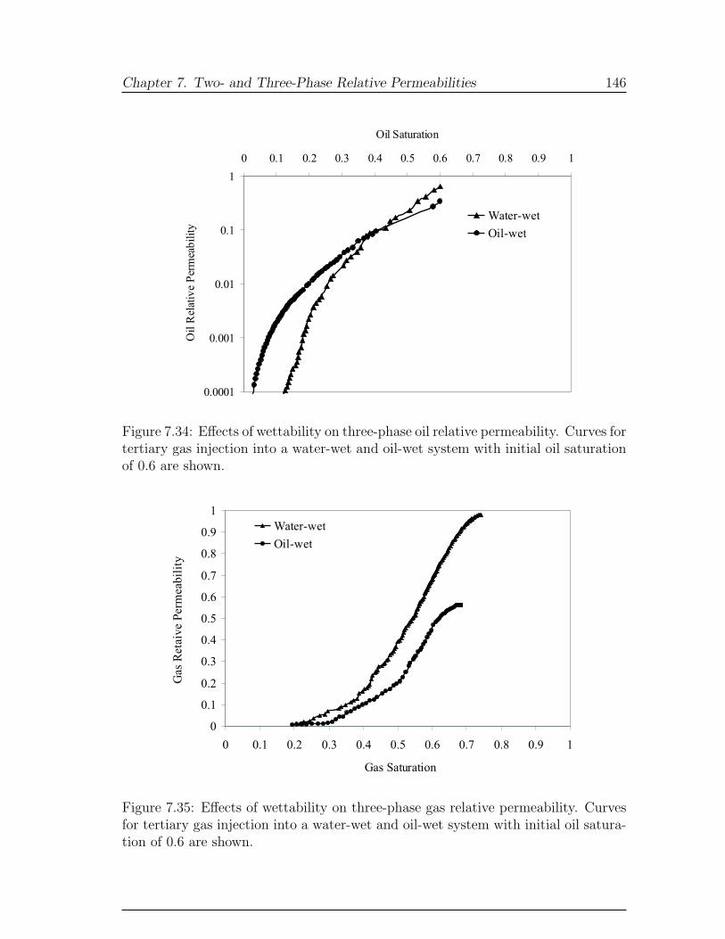
Chapter 7. Two- and Three-Phase Relative Permeabilities 146
0.0001
0.001
0.01
0.1
1
0 0.1 0.2 0.3 0.4 0.5 0.6 0.7 0.8 0.9 1
Oil Saturation
Oil
Rel
ativ
eP
erm
eab
ilit
y
Water-wet
Oil-wet
Figure 7.34: Effects of wettability on three-phase oil relative permeability. Curves fortertiary gas injection into a water-wet and oil-wet system with initial oil saturationof 0.6 are shown.
0
0.1
0.2
0.3
0.4
0.5
0.6
0.7
0.8
0.9
1
0 0.1 0.2 0.3 0.4 0.5 0.6 0.7 0.8 0.9 1
Gas Saturation
Gas
Ret
aive
Per
mea
bil
ity
Water-wet
Oil-wet
Figure 7.35: Effects of wettability on three-phase gas relative permeability. Curvesfor tertiary gas injection into a water-wet and oil-wet system with initial oil satura-tion of 0.6 are shown.
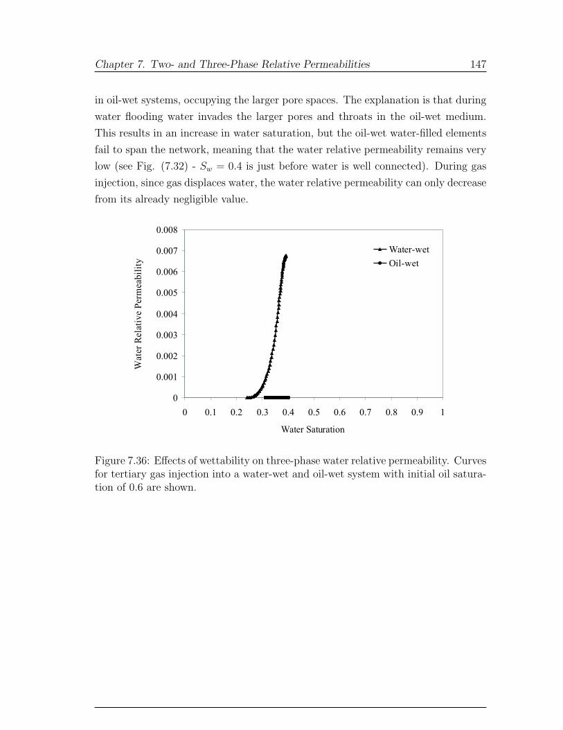
Chapter 7. Two- and Three-Phase Relative Permeabilities 147
in oil-wet systems, occupying the larger pore spaces. The explanation is that during
water flooding water invades the larger pores and throats in the oil-wet medium.
This results in an increase in water saturation, but the oil-wet water-filled elements
fail to span the network, meaning that the water relative permeability remains very
low (see Fig. (7.32) - Sw = 0.4 is just before water is well connected). During gas
injection, since gas displaces water, the water relative permeability can only decrease
from its already negligible value.
0
0.001
0.002
0.003
0.004
0.005
0.006
0.007
0.008
0 0.1 0.2 0.3 0.4 0.5 0.6 0.7 0.8 0.9 1
Water Saturation
Wat
erR
elat
ive
Per
mea
bil
ity
Water-wet
Oil-wet
Figure 7.36: Effects of wettability on three-phase water relative permeability. Curvesfor tertiary gas injection into a water-wet and oil-wet system with initial oil satura-tion of 0.6 are shown.
Chapter 8
Final Remarks
8.1 Conclusions
Based on today’s knowledge on physics of two- and three-phase flow in porous media
at the pore-level, a definitive capillary dominated three-phase network model was
developed that combines three essential components:
1. A description of the pore space and its connectivity that mimics real systems
2. A physically-based model of wettability alteration
3. A full description of fluid configurations for two- and three-phase flow
We described in detail how the model was developed and works. We also pre-
sented a novel and robust clustering algorithm to account for trapping and double
displacement. The model includes the following features:
• Mixed wettability
• Wetting layers
• Spreading layers
• Hysteresis and wettability alteration are fully accounted for. Any values of
receding and advancing oil/water, gas/water, and gas/oil contact angles can
be considered.
• Any random/regular two- and three-dimensional networks can be used.
• Direct two-phase displacements
148
Chapter 8. Final Remarks 149
• Layer reformation
• Double displacement
• Multiple injections
• Saturation tracking
The model successfully predicted two-phase water-wet relative permeabilities
measured on Berea sandstone by Oak [1]. For primary drainage there were no
parameters to adjust. For oil/water and gas/oil imbibition the advancing contact
angles were chosen to match the residual non-wetting phase saturation. Using these
contact angles excellent agreement between experiment and predictions was made.
For gas/water data we used a constraint, Eq. (2.6), to predict the gas/water contact
angles from the oil/water and gas/oil results. Again the match to experiment was
excellent.
We then predicted three-phase gas injection relative permeabilities from Oak [1].
We used a saturation tracking algorithm to follow exactly the same displacement
path as in the experiments. The predictions of gas and water relative permeabilities
and the oil relative permeability at high oil saturation were good. However, at
low oil saturations, where flow is dominated by spreading layers, we systematically
over-predicted the oil relative permeability. This was likely to be due to us over-
estimating the oil layer conductance.
We computed relative permeabilities for cases that had not been studied experi-
mentally. We showed that the oil relative permeability in tertiary gas injection – af-
ter water flooding – is lower than in secondary gas injection – after primary drainage,
since oil layers are less stable and thinner due to a low initial oil/water capillary pres-
sure. For secondary gas injection we observed an approximately quadratic variation
of oil relative permeability with oil saturation when flow was controlled by layers,
as seen experimentally. We then compared relative permeabilities of a tertiary gas
injection into water flood residual oil with those of a secondary gas injection with a
similar initial oil saturation. Oil relative permeability of the tertiary case was non-
zero and higher than that of the secondary gas injection at low oil saturations since
double-displacement caused an increase in oil/water capillary pressure – in tertiary
gas injection – leading to thicker and more conductive oil layers. The increase in the
oil/water capillary pressure also lowered gas and water relative permeabilities of the
tertiary case comparing to their secondary counterparts. These results were different
from the tertiary gas injection into oil that was initially already connected. We also
Chapter 8. Final Remarks 150
showed the effects of wettability on relative permeability by comparing tertiary gas
injection relative permeabilities for water-wet and oil-wet systems. The behaviour
of all three relative permeabilities was different from that observed in two-phase flow
and was explained in terms of the pore-scale physics.
The model could now be used to study a wide range of other phenomena in
three-phase flow, including water alternate gas (WAG) flooding and gas gravity
drainage.
8.2 Recommendations for Future Work
Still there is a great amount of work that can be done to improve, even further, the
abilities of the two- and three-phase pore-scale network models:
• More accurate layer conductance models for different boundary conditions
which are critically important for prediction of relative permeabilities at low
saturation
• Improved pore-body filling models
• Better estimations of three-phase equilibrium interfacial tensions
• More representative networks for different types of rocks, in particular carbon-
ates
Also there are many interesting subjects to be studied using three-phase network
modeling:
• Solution gas drive
• Effects of asphalt precipitation on three-phase relative permeabilities due to
composition variation, e.g. CO2 sequestration, or pressure drop below the
bubble point
• Gas condensates
• Coupling pore-scale network model to a 3D simulator to capture displacement
paths
• Dispersion in three-phase systems
• Water alternate gas (WAG) injection
Bibliography
[1] M. J. Oak. Three-phase relative permeability of water-wet Berea. Paper SPE
20183, Proceedings of the SPE/DOE Seventh Symposium on Enhanced Oil
Recovery, Tulsa, Oklahoma, 22-25 April, 1990.
[2] M. C. Leverett and W. B. Lewis. Steady flow of gas-oil-water mixtures through
unconsolidated sands. Transactions of the American Institute of Mining, Met-
allurgical, and Petroleum Engineers, 142(107):107–116, 1940.
[3] B. H. Caudle, R. L. Slobod, and E. R. Brownscombe. Further developments
in the laboratory determination of relative permeability. Transactions of the
American Institute of Mining, Metallurgical, and Petroleum Engineers, 192:
145–150, 1951.
[4] A. T. Corey, C. H. Rathjens, J. H. Henderson, and M. R. J. Wyllie. Three-
phase relative permeability. Transactions of the American Institute of Mining,
Metallurgical, and Petroleum Engineers, 207:349–351, 1956.
[5] J. Naar and R. J. Wygal. Three-phase imbibition relative permeability. SPE
Journal, December:254–258, 1961.
[6] R. W. Snell. Three phase relative permeability in an unconsolidated sand.
Journal of the Institute of Petroleum, 48:80–88, 1962.
[7] A. M. Sarem. Three-phase relative permeability measurement by unsteady-
state method. SPE Journal, September:199–205, 1966.
[8] E. C. Donaldson and G. W. Dean. Two- and three-phase relative permeability
studies. United States Department of the Interior Bureau of Mines, 6826:1–23,
1966.
[9] D. N. Saraf and I. Fatt. Three-phase relative permeability measurement using
nuclear magnetic resonance technique for estimating fluid saturation. SPE
Journal, September:235–242, 1967.
151
Bibliography 152
[10] D. N. Saraf, J. P. Batycky, C. H. Jackson, and D. B. Fisher. An experimental
investgation of three-phase flow of water-oil-gas mixtures through water-wet
sandstones. Paper SPE 10761, Proceedings of the SPE Regional Meeting, San
Francisco, CA, 24-26 March, 1982.
[11] E. V. Spronsen. Three-phase relative pemeability measurements using the
centrifuge method. Paper SPE 10688, Proceedings of the 3rd SPE/DOE joint
Symposium on Enhanced Oil Recovery, Tulsa, Oklahoma, 4-7 April, 1982.
[12] R. J. Lenhard and J. C. Parker. Measurement and prediction of saturation-
pressure relationships in three-phase porous media systems. Journal of Con-
taminant Hydrology, 1(4):407–424, 1987.
[13] A. S. Grader and D. J. O’Meara. Dynamic displacement measurements of
three-phase relative permeabilities using three immiscible liquids. Paper SPE
18293, Proceedings of the 63rd SPE Annual Technical Conference and Exhibi-
tion, Houston, TX, 2-5 October, 1988.
[14] R. J. Lenhard and J. C. Parker. Experimental validation of the theory of
extending two-phase saturation-pressure relations to three-fluid phase systems
for monotonic drainage paths. Water Resources Research, 24:373–380, 1988.
[15] B. B. Maini, S. Kokal, and K. Jha. Measurements and correlations of three-
phase relative permeability at elevated temperatures and pressures. Paper
SPE 19677, Proceedings of the 64th SPE Annual Technical Conference and
Exhibition, San Antonio, Texas, 8-11 October, 1989.
[16] M. J. Oak, L. E. Baker, and D. C. Thomas. Three-phase relative permeability
of Berea sandstone. Journal of Petroleum Technology, 42(8):1054–1061, 1990.
[17] B. B. Maini, F. Nicola, J. Goldman, and H. K. Sarma. Measurements and
estimation of three-phase relative permeability. Petroleum Recovery Institute,
Calgary, Canada, October, 1990.
[18] L. A. Ferrand, P. C. D. Milly, G. F. Pinder, and R. P. Turrin. A comparison
of capillary pressure-saturation relations for drainage in two- and three-fluid
porous media. Advances in Water Resources, 13(2):54–63, 1990.
[19] J. L. Wilson, S. H. Conrad, W. R. Mason, W. Peplinski, and E. Hagen. Labora-
tory investigation of residual liquid organics from spills, leaks and the disposal
Bibliography 153
of hazardous wastes in groundwater. EPA Report no. EPA/600/6-90/004,
EPA, Ada, OK, April, 1990.
[20] B. F. Marek, K. J. Hartman, and A. E. MacDonald. Three-phase relative
permeability of limestones having bimodal pore-size distribution. Paper SPE
21374, Proceedings of the SPE Middle East Oil Show held in Bahrain, 16-19
November, 1991.
[21] M. J. Oak. Three-phase relative permeability of intermediate-wet Berea sand-
stone. Paper SPE 22599, Proceedings of the 66th SPE Annual Technical Con-
ference and Exhibition, Dallas, TX, 6-9 October, 1991.
[22] R. J. Lenhard. Measurement and modeling of three-phase saturation-pressure
hysteresis. Journal of Contaminant Hydrology, 9(3):243–269, 1992.
[23] D. E. Dria, G. A. Pope, and K. Sepehrooni. Three-phase gas/oil/brine rela-
tive permeabilities measured under CO2 flooding conditions. SPE Reservoir
Engineering, 8(2):143–150, 1993.
[24] F. J. M. Kalaydjian, J. C. Moulu, O. Vizika, and P. K. Munkerud. Three-phase
flow in water-wet porous media:determination of gas/oil relative permeability
under various spreading conditions. Paper SPE 26671, Proceedings of the 68th
SPE Annual Technical Conference and Exhibition, Houston, TX, 3-6 October,
1993.
[25] J. E. Nordtvedt, E. Ebeltoft, J. E. Iversen, A. Sylte, H. Urkedal, K. O. Vatne,
and A. T. Watson. Determination of three-phase relative permeabilities from
displacement experiments. Paper SPE 36683, Proceedings of the SPE Annual
Technical Conference and Exhibition, Denver, Colorado, 6-9 October, 1996.
[26] S. Siddiqui, P. J. Hicks, and A. S. Grader. Verfication of buckley-leverett three-
phase theory using computerised tomography. Journal of Petroleum Science
and Engineering, 15(1):1–21, 1996.
[27] F. J. M. Kalaydjian, J. C. Moulu, O. Vizika, and P. K. Munkerud. Three-phase
flow in water-wet porous media: gas/oil relative permeabilities for various
spreading conditions. Journal of Petroleum Science and Engineering, 17(3-4):
275–290, 1997.
[28] E. J. Mackay, G. D. Henderson, D. H. Tehrani, and A. Danesh. The importance
of interfacial tension on fluid distribution during depressurisation. Paper SPE
Bibliography 154
38919, Proceedings of the SPE Annual Technical Conference and Exhibition,
San Antonio, Texas, 5-8 October, 1997.
[29] S. Siddiqui, J. Yang, and M. Ahmed. Dynamic displacement measurement
of three-phase relatrive permeabilities in berea sandstone cores. Paper SPE
49306, Proceedings of the SPE Annual Technical Conference and Exhibition,
New Orleans, Louisiana, 27-30 September, 1998.
[30] C. A. Grattoni, R. I. Hawes, and R. A. Dawe. Production of gas from
waterflood residual oil: gas saturation build-up and relative permeabilities.
Petroleum Geoscience, 7:131–136, 2001.
[31] M. Honarpour, L. Koederitz, and A. H. Harvey. Relative Permeability of
Petroleum Reservoirs. CRC Press, Florida, 1st edition, 1986.
[32] F. A. L. Dullien. Porous Media: Fluid Transport and Pore Structure. Academic
Press, San Diego, 2nd edition, 1992.
[33] M. C. Leverett. Capillary behaviour in porous solids. Transactions of the
American Institute of Mining, Metallurgical, and Petroleum Engineers, 142:
152–169, 1941.
[34] C. S. Land. Calculation of imbibition relative permeability for two- and three-
phase flow from rock properties. SPE Journal, June:149–156, 1968.
[35] H. L. Stone. Probability model for estimating three-phase relative permeabil-
ity. Journal of Petroleum Technology, 22(2):214–218, 1970.
[36] H. L. Stone. Estimation of three-phase relative permeability and residual oil
data. Journal of Canadian Petroleum Technology, 12(4):53–61, 1973.
[37] J. K. Dietrich and P. L. Bondor. Three-phase oil relative permeability models.
Paper SPE 6044, Proceedings of the 51st SPE Annual Technical Conference
and Exhibition, New Orleans, LA, 3-6 October, 1976.
[38] K. Aziz and A. Settari. Petroleum Reservoir Simulation. Elsevier Applied
Science, London, 1st edition, 1979.
[39] F. J. Fayers and J. D. Matthews. Evaluatin of normalized Stone’s method for
estimating three-phase relative permeabilities. SPE Journal, April:224–232,
1984.
Bibliography 155
[40] J. C. Parker, R. J. Lenhard, and T. Kuppusamy. A parametric model for
constitutive properties governing multiphase flow in porous media. Water
Resources Research, 23(4):618–624, 1987.
[41] J. C. Parker and R. J. Lenhard. A model for hysteretic constitutive relations
governing multiphase flow. 1.Saturation-pressure relations. Water Resources
Research, 23(12):2187–2196, 1987.
[42] R. J. Lenhard and J. C. Parker. A model for hysteretic constitutive rela-
tions governing multiphase flow. 2.Permeability-saturation relations. Water
Resources Research, 23(12):2197–2206, 1987.
[43] L. E. Baker. Three-phase relative permeability correlations. Paper SPE 17369,
Proceedings of the SPE/DOE Enhanced Oil Recovery Symposium, Tulsa, Ok-
lahoma, 17-20 April, 1988.
[44] M. A. Aleman and J. C. Slattery. Estimation of three-phase relative perme-
abilities. Transport in Porous Media, 3(2):111–131, 1988.
[45] F. J. Fayers. Extension of stone’s method i and conditions for real character-
istics in three-phase flow. SPE Reservoir Engineering, 4:437–445, 1989.
[46] M. Delshad and G. A. Pope. Comparison of the three-phase oil relative per-
meability models. Transport in Porous Media, 4(1):59–83, 1989.
[47] J. C. Parker and R. J. Lenhard. Determining three-phase permeability-
saturation-pressure relations from two-phase measurements. Journal of
Petroleum Science and Engineering, 4:57–65, 1990.
[48] O. S. Hustad and A. G. Hansen. A consistent correlation for three-phase rela-
tive permeabilities and phase pressures based on three sets of two-phase data.
Proceedings of the Eightth European Symposium on Improved Oil Recovery,
Vienna, 15-17 May, 1995.
[49] G. R. Jerauld. General three-phase relative permeability model for Purdhoe
Bay. Paper SPE 36178, Proceedings of the 7th ADIPEC, Abu Dhabi, 13-16
October, 1996.
[50] G. R. Jerauld. Prudhoe Bay gas/oil relative permeability. SPE Reservoir
Engineering, 12(1):66–73, 1997.
Bibliography 156
[51] E. F. Balbinski, T. P. Fishlock, S. G. Goodyear, and P. I. R. Jones. Key char-
acteristics of three-phase oil relative permeability formulations for improved
oil recovery predictions. Petroleum Geoscience, 5(4):339, 1999.
[52] F. J. Fayers. An improved three-phase flow model incorporating composi-
tional variance. Paper SPE 59313, Proceedings of the SPE/DOE Improved
Oil Recovery Symposium, Tulsa, Oklahoma, 3-5 April, 2000.
[53] M. J. Blunt. An empirical model for three-phase relative permeability. SPE
Journal, 5(4):435–445, 2000.
[54] O. S. Hustad. A coupled model for three-phase capillary pressure and relative
permeability. SPE Journal, 7(1):59–69, 2002.
[55] M. J. Blunt. Pore level modeling of the effects of wettability. SPE Journal,
2(4):494–510, 1997.
[56] G. G. Pereira, W. V. Pinczewski, D. Y. C. Chan, L. Paterson, and P. E. Øren.
Pore-scale network model for drainage-dominated three-phase flow in porous
media. Transport in Porous Media, 24(2):167–201, 1996.
[57] R. Lenormand, C. Zarcone, and A. Sarr. Mechanisms of the displacement
of one fluid by another in a network of capillary ducts. Journal of Fluid
Mechanics, 135(October):337–353, 1983.
[58] R. Lenormand and C. Zarcone. Role of roughness and edges during imbibition
in square capillaries. Paper SPE 13264, Proceedings of the 59th SPE Annual
Technical Conference and Exhibition, Houston, TX, 16-19 September, 1984.
[59] J. D. Chen and J. Koplik. Immiscible fluid displacement in small networks.
Journal of Colloid and Interface Science, 108(2):304–330, 1985.
[60] I. Chatzis, A. Kantzas, and F. A. L. Dullien. On the investigation of gravity-
assisted inert gas injection using micromodels, long Berea sandstone cores,
and computer-assisted tomography. Paper SPE 18284, Proceedings of the 63rd
SPE Annual Technical Conference and Exhibition, Houston, TX, 2-5 October,
1988.
[61] A. Kantzas, I. Chatzis, and F. A. L. Dullien. Mechanisms of capillary displace-
ment of residual oil by gravity-assisted inert gas injection. Paper SPE 17506,
Proceedings of the SPE Rocky Mountain Regional Meeting, Casper, WY, 11-13
May, 1988.
Bibliography 157
[62] A. Kantzas, I. Chatzis, and F. A. L. Dullien. Enhanced oil recovery by inert
gas injection. Paper SPE 17379, Proceedings of the SPE/DOE Enhanced Oil
Recovery Symposium, Tulsa, Oklahoma, 17-20 April, 1988.
[63] P. E. Øren and W. V. Pinczewski. The effect of film-flow on the mobilization
of waterflood residual oil by gas flooding. Proceedings of the 6th European
IOR Symposium, Stavanger, May, 1991.
[64] P. E. Øren and W. V. Pinczewski. Mobilization of waterflood residual oil by
gas injecton for water wet conditions. SPE Formation Evaluation, 7:70–78,
1992.
[65] P. E. Øren and W. V. Pinczewski. The effect of wettability and spreading
coefficients on the recovery of waterflood residual oil by immiscible gasflooding.
Paper SPE 24881, Proceedings of the 67th SPE Annual Technical Conference
and Exhibition, Washington, DC, 4-7 October, 1992.
[66] W. E. Soll, M. A. Celia, and J. L. Wilson. Micromodel studies of three-
fluid porous media systems: pore-scale processes relating to capillary pressure-
saturation relationships. Water Resources Research, 29(9):2963–2974, 1993.
[67] P. E. Øren and W. V. Pinczewski. Effect of wettability and spreading coeffi-
cients on recovery of waterflood residual oil by immiscible gasflooding. SPE
Formation Evaluation, 9(2):149–156, 1994.
[68] M. J. Blunt, D. Zhou, and D. H. Fenwick. Three-phase flow and gravity
drainage in porous media. Transport in Porous Media, 20(1-2):77–103, 1995.
[69] P. E. Øren and W. V. Pinczewski. Fluid ditribution and pore-scale displace-
ment mechanisms in drainage dominaed three-phase flow. Transport in Porous
Media, 20(1-2):105–133, 1995.
[70] M. Dong, F. A. L. Dullien, and I. Chatzis. Imbibition of oil in film form over
water present in edges of capillaries with an angular cross section. Journal of
Colloid and Interface Science, 172(1):21–36, 1995.
[71] O. Vizika and J. M. Lombard. Wettability and spreading: Two key parameters
in oil recovery with three-phase gravity drainage. SPE Reservoir Engineering,
11(1):54–60, 1996.
Bibliography 158
[72] A. A. Keller, M. J. Blunt, and P. V. Roberts. Micromodel observation of
the role of oil layers in three-phase flow. Transport in Porous Media, 26(3):
277–297, 1997.
[73] P. M. Adler, C. G. Jacquin, and J. A. Quiblier. Flow in simulated porous
media. International Journal of Multiphase Flow, 16(4):691–712, 1990.
[74] A. P. Roberts. Statistical reconstruction of three-dimesional porous media
from two-dimensional images. Physical Review E, 56(3):3203–3212, 1997.
[75] C. L. Y. Yeong and S. Torquato. Reconstructing random media II. three-
dimensional media from two-dimensinal cuts. Physical Review E, 58(1):224–
233, 1998.
[76] S. Bakke and P. E. Øren. 3-D pore-scale modelling of sandstones and flow
simulations in the pore networks. SPE Journal, 2(2):136–149, 1997.
[77] P. E. Øren, S. Bakke, and O. J. Arntzen. Extending predictive capabilities to
network models. SPE Journal, 3(4):324–336, 1998.
[78] P. E. Øren and S. Bakke. Process based reconstruction of sandstones and
prediction of transport properties. Transport in Porous Media, 46(2-3):311–
343, 2002.
[79] J. H. Dunsmuir, S. R. Ferguson, K. L. D’Amico, and J. P. Stokes. X-ray
microtomography: a new tool for the characterization of porous media. Paper
SPE 22860, Proceedings of the 66th SPE Annual Technical Conference and
Exhibition, Dallas, TX, 6-9 October, 1991.
[80] P. Spanne, J. F. Thovert, C. J. Jacquin, W. B. Lindquist, K. W. Jones, and
P. M. Adler. Synchrotron computed microtomography of porous media: topol-
ogy and transports. Physical Review Letters, 73(14):2001–2004, 1994.
[81] A. K. Gunstensen, D. H. Rothman, S. Zaleski, and G. Zanetti. Lattice boltz-
mann model of immiscible fluids. Physical Review A, 43(8):4320–4327, 1991.
[82] D. Grunau, S. Chen, and K. Eggert. A lattice boltzmann model for multiphase
fluid flows. Physics of Fluids A - Fluid Dynamics, 5(10):2557–2562, 1993.
[83] B. Ferreol and D. H. Rothman. Lattice-Boltzmann simulations of flow through
Fontainebleau porous media. Transport in Porous Media, 20(1-2):3–20, 1995.
Bibliography 159
[84] F. M. Van Katz and P. J. P. Egberts. Simulation of three-phase displacement
mechanisms using a 2D Lattice-Boltzmann model. Transport in Porous Media,
37(1):55–68, 1999.
[85] J. F. Delerue and E. Perrier. Dxsoil, a library for 3d image analysis in soil
science. Computational Geosciences, 28(9):1041–1050, 2002.
[86] I. Fatt. The network model of porous media I. capillary pressure character-
istics. Transactions of the American Institute of Mining, Metallurgical, and
Petroleum Engineers, 207:144–159, 1956.
[87] I. Fatt. The network model of porous media II. dynamic properties of a
single size tube network. Transactions of the American Institute of Mining,
Metallurgical, and Petroleum Engineers, 207:160–163, 1956.
[88] I. Fatt. The network model of porous media III. dynamic properties of net-
works with tube radius distribution. Transactions of the American Institute
of Mining, Metallurgical, and Petroleum Engineers, 207:164–181, 1956.
[89] M. A. Celia, P. C. Reeves, and L. A. Ferrand. Recent advances in pore scale
models for multiphase flow. Reviews of Geophysics, Supplement, 33:1049–
1057, 1995.
[90] M. J. Blunt. Flow in porous media- pore-network models and multiphase flow.
Current Opinion in Colloid and Interface Science, 6(3):197–207, 2001.
[91] M. J. Blunt, M. D. Jackson, M. Piri, and P. H. Valvatne. Detailed physics,
predictive capabilities and macroscopic consequences for pore-network models
of multiphase flow. Advances in Water Resources, 25(8-12):1069–1089, 2002.
[92] K. K. Mohanty and S. J. Salter. Multiphase flow in porous media:II Pore-level
modeling. Paper SPE 11018, Proceedings of the 57th SPE Annual Fall Tech-
nical Conference and Exhibition, New Orleans, LA, 26-29 September, 1982.
[93] C. Y. Lin and J. C. Slattery. 3-dimensional, randomized, network model for
two phase flow through porous-media. AIChE Journal, 28(2):311–324, 1982.
[94] R. Chandler, J. Koplik, K. Lerman, and J. F. Willemsen. Capillary displace-
ment and percolation in porous media. Journal of Fluid Mechanics, 119(June):
249–267, 1982.
Bibliography 160
[95] K. K. Mohanty and S. J. Salter. Multiphase flow in porous media:III Oil
mobilization, Transverse dispersion, and Wettability. Paper SPE 12127, Pro-
ceedings of the 58th SPE Annual Technical Conference and Exhibition, San
Francisco, CA, 5-8 October, 1983.
[96] A. A. Heiba, H. T. Davis, and L. E. Scriven. Effect of wettability on two-phase
relative permeabilities and capillary pressures. Paper SPE 12172, Proceedings
of the 58th SPE Annual Technical Conference and Exhibition, San Francisco,
CA, 5-8 October, 1983.
[97] J. Koplik and T. J. Lasseter. Two-phase flow in random network models of
porous media. SPE Journal, February:89–100, 1985.
[98] A. A. Heiba, G. R. Jerauld, H. T. Davis, and L. E. Scriven. Mechanism-based
simulation of oil recovery processes. Paper SPE 15593, Proceedings of the
61st SPE Annual Technical Conference and Exhibition, New Orleans, LA, 5-8
October, 1986.
[99] M. M. Dias and A. C. Payatakes. Network models for two-phase flow in porous
media. Part 1. immiscible micro-displacements of non-wetting fluids. Journal
of Fluid Mechanics, 164:305–336, 1986.
[100] C. E. Diaz, I. Chatzis, and F. A. L. Dullien. Simulation of capillary pres-
sure curves using bond correlated site percolation on a simple cubic network.
Transport in Porous Media, 2(3):215–240, 1987.
[101] J. Bear, C. Braester, and P. C. Menier. Effective and relative permeabilities
of anisotropic porous media. Transport in Porous Media, 2:301–316, 1987.
[102] R. Lenormand, E. Touboul, and C. Zarcone. Numerical models and exper-
iments on immiscible displacements in porous media. Journal of Fluid Me-
chanics, 189(April):165–187, 1988.
[103] D. Y. C. Chan, B. D. Hughes, and L. Paterson. Simulating flow in porous
media. Physical Review A, 38(8):4106–4120, 1988.
[104] G. R. Jerauld and S. J. Salter. The effect of pore structure on hysteresis in
relative permeability and capillary pressure: Pore-level modelling. Transport
in Porous Media, 5(2):102–151, 1990.
Bibliography 161
[105] M. J. Blunt and P. King. Relative permeabilities from two- and three-
dimensional pore-scale network modelling. Transport in Porous Media, 6:
407–433, 1991.
[106] M. J. Blunt, M. J. King, and H. Scher. Simulation and theory of two-phase
flow in porous media. Physical Review A, 46:7680–7699, 1992.
[107] S. Bryant and M. J. Blunt. Prediction of relative permeability in simple porous
media. Physical Review A, 46(4):2004–2011, 1992.
[108] A. A. Heiba, M. Sahimi, L. E. Scriven, and H. T. Davis. Percolation theory of
two-phase relative permeability. SPE Reservoir Engineering, 7:123–132, 1992.
[109] J. A. Billiotte, H. DeMoegen, and P. E. Øren. Experimental micromodeling
and numerical simulation of gas/water injection/withdrawal cycles as applied
to underground gas storage reservoirs. SPE Aadvanced Technology Series,
1(1):133–139, 1993.
[110] M. A. Ioannidis and I. Chatzis. A mixed-percolation model of capillary hystere-
sis and entrapment in mercury porosimetry. Journal of Colloid and Interface
Science, 161:278–291, 1993.
[111] S. L. Bryant, D. W. Mellor, and C. A. Cade. Physically representative network
models of transport in porous media. AIChE Journal, 39(3):387–396, 1993.
[112] P. A. Goode and T. S. Ramakrishnan. Momentum transfer across fluid-fluid
interfaces in porous media: a network model. AIChE Journal, 39(7):1124–
1134, 1993.
[113] S. R. McDougall and K. S. Sorbie. The impact of wettability on waterflooding:
Pore-scale simulation. SPE Reservoir Engineering, 10(3):208–213, 1995.
[114] M. I. Lowry and C. T. Miller. Pore-scale modeling of nonwetting-phase residual
in porous media. Water Resources Research, 31(3):455–473, 1995.
[115] S. H. Lee, L. Padmanabhan, and H. A. Al-Sunaidi. Simulation of linear dis-
placement experiments on massively parallel computers. Paper SPE 30721,
Proceedings of the SPE Annual Technical Conference and Exhibition, Dallas,
TX, 22-25 October, 1995.

Bibliography 162
[116] P. C. Reeves and M. A. Celia. A functional relationship between capillary
pressure, saturation, and interfacial area as revealed by a pore-scale network
model. Water Resources Research, 32(8):2345–2358, 1996.
[117] L. Paterson, S. Painter, X. Zhang, and W. V. Pinczewski. Simulation residual
saturation and relative permeability in heterogeneous formations. Paper SPE
36523, Proceedings of the SPE Annual Technical Conference and Exhibition,
Denver, Colorado, 6-9 October, 1996.
[118] L. S. Nilsen, P. E. Øren, S. Bakke, and A. Henriquez. 3-D pore-scale modelling
of heterogeneous sandstone reservoir rocks and quantitative analysis of the
architecture, geometry and spatial continuity of the pore network. Paper SPE
35531, in Proceedings of the European 3-D Reservoir Modelling Conference,
Stavanger, Norway, 16-17 April, 1996.
[119] M. J. Blunt. Effects of heterogeneity and wetting on relative permeability
using pore level modeling. SPE Journal, 2:70, 1997.
[120] A. B. Dixit, S. R. McDougall, and K. S. Sorbie. A pore-level investigation of
relative permeability hysteresis in water-wet systems. Paper SPE 37233, Pro-
ceedings of the SPE International Symposium on Oilfield Chemistry, Houston,
Texas, 18-21 February, 1997.
[121] H. Rajaram, L. A. Ferrand, and M. A. Celia. Prediction of relative permeabili-
ties for unconsolidated soils using pore-scale network models. Water Resources
Research, 33(1):43–52, 1997.
[122] A. S. Dixit, S. R. McDougall, K. S. Sorbie, and J. S. Buckley. Pore-scale mod-
elling of wettability effects and their influence on oil recovery. SPE Reservoir
Evaluation and Engineering, 2(1):25–36, 1999.
[123] U. Fischer and M. A. Celia. Prediction of relative and absolute permeabilities
for gas and water from soil water retention curves using a pore-scale network
model. Water Resources Research, 35(4):1089–1100, 1999.
[124] B. Xu, J. Kamath, Y. C. Yortsos, and S. H. Lee. Use of pore-network models
to simulate laboratory coreflods in a heterogeneous carbonate sample. SPE
Journal, 4(3):179–186, 1999.
[125] C. Laroche, O. Vizika, and F. Kalaydjian. Network modeling to predict the
effect of wettability heterogeneities on multiphase flow. Paper SPE 56674,
Bibliography 163
Proceedings of the SPE Annual Technical Conference and Exhibition, Houston,
TX, 3-6 October, 1999.
[126] A. Maximenko and V. V. Kadet. Determination of relative permeabilities
using the network models of porous media. Journal of Petroleum Science and
Engineering, 28(3):145–152, 2000.
[127] T. W. Patzek. Verification of a complete pore network simulator of drainage
and imbibition. SPE Journal, 6(2):144–156, 2001.
[128] M. A. Knackstedt, A. P. Sheppard, and M. Sahimi. Pore network modelling of
two-phase flow in porous rock: the effect of correlated heterogeneity. Advances
in Water Resources, 24(3-4):257–277, 2001.
[129] R. J. Held and M. A. Celia. Modeling support of functional relationships
between capillary pressure, saturation, interfacial area and common lines. Ad-
vances in Water Resources, 24(3-4):325–343, 2001.
[130] M. Hilpert and C. T. Miller. Pore-morphology-based simulation of drainage
in totally wetting porous media. Advances in Water Resources, 24:243–255,
2001.
[131] R. J. Held and M. A. Celia. Pore-scale modeling extension of constitutive
relationships in the range of residual saturations. Water Resources Research,
37(1):165–170, 2001.
[132] M. Piri and M. J. Blunt. Pore-scale modeling of three-phase flow in mixed-wet
systems. Paper SPE 77726, Proceedings of the SPE Annual Technical Confer-
ence and Exhibition, San Antonio, Texas, 29 September-2 October, 2002.
[133] M. Ferer, G. S. Bromhal, and D. H. Smith. Pore-level modeling of drainage:
Crossover from inavsion percolasion fingering to compact flow. Physical Review
E, 67:051601.1–051601.12, 2003.
[134] P. H. Valvatne and M. J. Blunt. Predictive pore-scale modeling of two-phase
flow in mixed-wet media. Submitted to Water Resources Research, , 2003.
[135] P. H. Valvatne and M. J. Blunt. Predictive pore-scale network modeling.
Paper SPE 84550, Proceedings of the SPE Annual Technical Conference and
Exhibition, Denver, Colorado, 5-8 October, 2003.
Bibliography 164
[136] P. E. Øren and S. Bakke. Reconstruction of Berea sandstone and pore-scale
modelling of wettability. Journal of Petroleum Science and Engineering, 39(3-
4):177–199, 2003.
[137] A. Al-Futaisi and T. W. Patzek. Impact of wettability alteration on two-phase
flow characteristics of sandstones: A quasi-static description. Water Resources
Research, 39(2)(SBH12):1–13, 2003.
[138] A. A. Heiba, H. T. Davis, and L. E. Scriven. Statistical network theory of three-
phase relative permeabilities. Paper SPE 12690, Proceedings of the SPE/DOE
Symposium on Enhanced Oil Recovery, Tulsa, Oklahoma, 15-18 April, 1984.
[139] W. E. Soll and M. A. Celia. A modified percolation approach to simulat-
ing three-fluid capillary pressure-saturation relationships. Advances in Water
Resources, 16:107–126, 1993.
[140] P. E. Øren, J. Billiotte, and W. V. Pinczewski. Pore-scale network modelling
of waterflood residual oil recovery by immiscible gas flooding. Paper SPE
27814, Proceedings of the SPE/DOE Symposium in Improved Oil Recovery,
Tulsa, Oklahoma, 17-20 April, 1994.
[141] L. Paterson, J. Y. Lee, and W. V. Pinczewski. Three-phase relative perme-
ability in heterogeneous formations. Paper SPE 38882, Proceedings of the
SPE Annual Technical Conference and Exhibition, San Antonio, Texas, 5-8
October, 1997.
[142] D. H. Fenwick and M. J. Blunt. Three-dimensional modeling of three phase
imbibition and drainage. Advances in Water Resources, 21(2):121–143, 1998.
[143] D. H. Fenwick and M. J. Blunt. Network modeling of three-phase flow in
porous media. SPE Journal, 3(1):86–97, 1998.
[144] V. Mani and K. K. Mohanty. Effect of the spreading coefficient on three-phase
flow in porous media. Journal of Colloid and Interface Science, 187(1):45–56,
1997.
[145] V. Mani and K. K. Mohanty. Pore-level network modeling of three-phase
capillary pressure and relative permeability curves. SPE Journal, 3:238–248,
1998.
Bibliography 165
[146] C. Laroche, O. Vizika, and F. Kalaydjian. Network modeling as a tool to
predict three-phase gas injection in heterogeneous wettability porous media.
Journal of Petroleum Science and Engineering, 24(2-4):155–168, 1999.
[147] G. G. Pereira. Numerical pore-scale modeling of three-phase fluid
flow:Comparison between simulation and experiment. Physical Review E,
59(4):4229–4242, 1999.
[148] J. C. Moulu, O. Vizika, P. Egermann, and F. Kalaydjian. A new three-phase
relative permeability model for various wettability conditions. Paper SPE
56477, Proceedings of the SPE Annual Technical Conference and Exhibition,
Houston, TX, 3-6 October, 1999.
[149] T. R. Lerdahl, P. E. Øren, and S. Bakke. A predictive network model for three-
phase flow in porous media. Paper SPE 59311, Proceedings of the SPE/DOE
Symposium in Improved Oil Recovery, Tulsa, Oklahoma, 3-5 April, 2000.
[150] J. K. Larsen, N. Bech, and A. Winter. Three-phase immiscible WAG injection:
micromodel experiments and network models. Paper SPE 59324, Proceedings
of the SPE/DOE Improved Oil Recovery Symposium, Tulsa, Oklahoma, 3-5
April, 2000.
[151] M. I. J. van Dijke, K. S. Sorbie, and S. R. McDougall. A process-based
approach for three-phase capillary pressure and relative permeability relation-
ships in mixed-wet systems. Paper SPE 59310, Proceedings of the SPE/DOE
Symposium in Improved Oil Recovery, Tulsa, Oklahoma, 3-5 April, 2000.
[152] M. I. J. van Dijke, K. S. Sorbie, and S. R. McDougall. Saturation-dependencies
of three-phase relative permebilities in mixed-wet and fractionally wet systems.
Advances in Water Resources, 24:365–384, 2001.
[153] M. I. J. van Dijke, S. R. McDougall, and K. S. Sorbie. Three-phase cap-
illary pressure and relative permeability relationships in mixed-wet systems.
Transport in Porous Media, 44:1–32, 2001.
[154] M. I. J. van Dijke, K. S. Sorbie, M. Sohrabi, D. Tehrani, and A. Danesh.
Three-phase flow in WAG processes in mixed-wet porius media: pore-scale
network simulations and comparison with micromodel experiments. Paper
SPE 75192, Proceedings of the SPE/DOE Tenth Symposium on Improved Oil
Recovery, Tulsa, Oklahoma, 13-17 April, 2002.
Bibliography 166
[155] M. I. J. van Dijke and K. S. Sorbie. Pore-scale network model for three-phase
flow in mixed-wet porous media. Physical Review E, 66:046302.1–046302.14,
2002.
[156] N. Silpngarmlers and T. Ertekin. Artificial neural network architectures for
predicting two-phase and three-phase relative permeabilitiy characteristics.
Paper SPE 77704, Proceedings of the SPE Annual Technical Conference and
Exhibition, San Antonio, Texas, 29 September-2 October, 2002.
[157] B. Guler, T. Ertekin, and A. S. Grader. An artificial neural network based
relative permeability predictor. Paper 9991, Proceedings of the 8th Petroleum
Conference of the South Saskatchewan Section, The Petroleum Society of CIM,
Regina, 18-21 October, 1999.
[158] N. Silpngarmlers, B. Guler, T. Ertekin, and A. S. Grader. Development
and testing of two-phase relative permeability predictrs using artificial neu-
ral networks. Paper SPE 69392, Proceedings of the SPE Latin American and
Caribbean Petroleum Engineering Conference, Buenos Aires, Argentina, 25-28
March, 2001.
[159] G. P. Androutsopoulos and R. Mann. Evaluation of mercury porosimetry using
a network pore structure model. Chemical Engineering Science, 34:1203–1212,
1979.
[160] I. Chatzis and F. A. L. Dullien. The modeling of mercury porosimetry and
relative permeability of mercury in sandstones using percolation theory. Int.
Chem. Eng., 25:47–65, 1985.
[161] C. D. Tsakiroglou and A. C. Payatakes. A new simulator of mercury porosime-
try for the characterization of the porous materials. Journal of Colloid and
Interface Science, 137:315–339, 1990.
[162] P. G. Toledo, L. E. Scriven, and H. T. Davis. Pore-space statistics and cap-
illary pressure curves from volume-controlled porosimetry. SPE Formation
Evaluation, 9(1):46–54, 1994.
[163] C. D. Tsakiroglou and A. C. Payatakes. Characterization of the pore structure
of reservoir rocks with the aid of serial sectioning analysis, mercury porosime-
try and network simulation. Advances in Water Resources, 23(7):773–789,
2000.
Bibliography 167
[164] Y. Li, W. G. Laidlaw, and N. C. Wardlaw. Sensitivity of drainage and imbi-
bition to pore structures as revealed by computer simulation of displacement
process. Advances in Colloid and Interface Science, 26:1–68, 1986.
[165] C. D. Tsakiroglou and M. Fleury. Resistivity index of frcational wettability
porous media. Journal of Petroleum Science and Engineering, 22:253–274,
1999.
[166] H. N. Man and X. D. Jing. Network modelling of wettability and pore geometry
effects on electrical resistivity and capillary pressure. Journal of Petroleum
Science and Engineering, 24(2-4):255–267, 1999.
[167] C. D. Tsakiroglou and M. Fleury. Pore network analysis of resistivity index
for water-wet porous media. Transport in Porous Media, 35(1):89–128, 1999.
[168] H. N. Man and X. D. Jing. Pore network modelling of electrical resistivity and
capillary pressure characteristics. Transport in Porous Media, 41(3):263–286,
2000.
[169] H. N. Man and X. D. Jing. Network modelling of strong and intermediate
wettability on electrical resistivity and capillary pressure. Advances in Water
Resources, 24(3-4):345–363, 2001.
[170] H. N. Man and X. D. Jing. Network modelling of mixed-wettability on electri-
cal resistivity, capillary pressure and wettability indices. Journal of Petroleum
Science and Engineering, 33(1-3):101–122, 2002.
[171] R. P. Ewing and B. Berkowitz. A generalized growth model for simulating ini-
tial migration of dense non-aqueous phase liquids. Water Resources Research,
34(4):611–622, 1998.
[172] C. Jia, K. Shing, and Y. C. Yortsos. Visualization and simulation of non-
aqueous phase liquids solubilization in pore networks. Journal of Contaminant
Hydrology, 35(4):363–387, 1999.
[173] C. Jia, K. Shing, and Y. C. Yortsos. Advective mass transfer from stationary
sources in porous media. Water Resources Research, 35(11):3239–3251, 1999.
[174] D. Zhou, L. A. Dillard, and M. J. Blunt. A physically based model of dissolu-
tion of nonaqueous phase liquids in the saturated zone. Transport in Porous
Media, 39(2):227–255, 2000.
Bibliography 168
[175] L. A. Dillard and M. J. Blunt. Development of a pore network simulation
model to study nonaqueous phase liquid dissolution. Water Resources Re-
search, 36(2):439–454, 2000.
[176] A. Ahamdi, A. Aigueperse, and M. Quintard. Calculation of the effective
properties decribing active dispersion in porous media: from simple to complex
unit cells. Advances in Water Resources, 24:423–438, 2001.
[177] L. A. Dillard, H. I. Essaid, and M. J. Blunt. A functional relation for field-scale
nonaqueous phase liquid dissolution developed using a pore network model.
Journal of Contaminant Hydrology, 48(1-2):89–119, 2001.
[178] R. J. Held and M. A. Celia. Pore-scale modeling and upscaling of nonaqueous
phase liquid mass transfer. Water Resources Research, 37(3):539–549, 2001.
[179] C. E. Knutson, C. J. Werth, and A. J. Valocchi. Pore-scale modeling of
dissolution from variably distributed nonaqueous phase liquid blobs. Water
Resources Research, 37(12):2951–2963, 2001.
[180] C. Satik and Y. C. Yortsos. A pore network study of bubble growth in porous
media driven by heat transfer. Journal of Heat Transfer, 118:455–462, 1995.
[181] X. Li and Y. C. Yortsos. Theory of multiple bubble growth in porous media
by solute diffusion. Chemical Engineering Science, 50(8):1247–1271, 1995.
[182] C. Du and Y. C. Yortsos. A numerical study of the critical gas saturation in
a porous media. Transport in Porous Media, 35(2):205–225, 1999.
[183] R. Bora, B. B. Maini, and A. Chakma. Flow visualization studies of solu-
tion gas drive process in heavy oil reservoirs with a glass micromodel. SPE
Reservoir Evaluation and Engineering, 3(3):224–229, 2000.
[184] M. E. Kainourgiakis, A. K. Stubos, N. D. Konstantinou, N. K. Kanellopoulos,
and V. Milisic. A network model for the permeability of condensable vapours
through mesoporous media. Journal of Membrane Science, 114:215–225, 1996.
[185] X. Wang and K. K. Mohanty. Critical condensate saturation in porous media.
Journal of Colloid and Interface Science, 214:416–426, 1999.
[186] X. Wang and K. K. Mohanty. Pore-network model of flow in gas/condensate
reservoirs. SPE Journal, 5(4):426–434, 2000.
Bibliography 169
[187] M. Jamiolahmady, A. Danesh, D. H. Tehrani, and D. B. Duncan. A mecha-
nistic model of gas-condensate flow in pores. Transport in Porous Media, 41:
17–46, 2000.
[188] M. Jamiolahmady, A. Danesh, D. H. Tehrani, and D. B. Duncan. Positive
effect of flow velocity on gas-condensate relative permeability: network mod-
elling and comparison with experimental rsults. Transport in Porous Media,
52:159–183, 2003.
[189] M. Prat. Isothermal drying of non-hygroscopic capillary-porous materials as
an invasion percolation process. International Journal of Multiphase Flow,
21(5):875–892, 1995.
[190] J. B. Laurindo and M. Prat. Numerical and experimental network study of
evaporation in capillary porous media. Phase Distribution. Chemical Engi-
neering Science, 51(23):5171–5185, 1996.
[191] J. B. Laurindo and M. Prat. Numerical and experimental network study of
evaporation in capillary porous media.Drying rates. Chemical Engineering
Science, 53(12):2257–2269, 1996.
[192] I. N. Tsimpanogiannis and Y. C. Yortsos. Scaling theory of drying in porous
media. Physical Review E, 59(4):4353–4365, 1999.
[193] A. G. Yiotis, A. K. Stubos, A. G. Boudouvis, and Y. C. Yortsos. A 2-D pore-
network model of the drying of single-component liquids in porous media.
Advances in Water Resources, 24:439–460, 2001.
[194] M. Prat. Recent advances in pore-scale models for drying of porous media.
Chemical Engineering Journal, 86(1-2):153–164, 2002.
[195] F. Plourde and M. Prat. Pore network simulations of drying of capillay porous
media. influence of thermal gradients. International Journal of Heat and Mass
Transfer, 46(7):1293–1307, 2003.
[196] D. S. Freitas and M. Prat. Pore network simulation of evaporation of a binary
liquid from a capillary porous medium. Transport in Porous Media, 40:1–25,
2000.
[197] J. Carmeliet, F. Descamps, and G. Houvenaghel. A multiscale network model
for simulating moisture transfer properties of porous media. Transport in
Porous Media, 35(1):67–88, 1999.
Bibliography 170
[198] K. Mogensen and E. Stenby. A dynamic pore-scale model of imbibition. Paper
SPE 39658, Proceedings of the SPE/DOE Symposium in Improved Recovery,
Tulsa, Oklahoma, 19-22 April, 1998.
[199] E. Aker, K. J. Maløy, A. Hansen, and G. G. Batrouni. A two-dimensional
networksimulator for two-phase flow in porous media. Transport in Porous
Media, 32(2):163–186, 1998.
[200] K. Mogensen and E. Stenby. A dynamic two-phase pore-scale model of imbi-
bition. Transport in Porous Media, 32(3):299–327, 1998.
[201] H. K. Dahle and M. A. Celia. A dynamic network model for two-phase im-
miscible flow. Computational Geosciences, 3(1):1–22, 1999.
[202] K. Mogensen, E. Stenby, S. Banerjee, and V. A. Barker. Comparison of iter-
ative methods for computing the pressure field in a dynamic network model.
Transport in Porous Media, 37:277–301, 1999.
[203] R. G. Hughes and M. J. Blunt. Pore scale modeling of rate effects in imbibition.
Transport in Porous Media, 40(3):295–322, 2000.
[204] G. N. Constantinides and A. C. Payatakes. Effects of precursor wetting films
in immiscible displacement through porous media. Transport in Porous Media,
38(3):291–317, 2000.
[205] M. S. Valavanides and A. C. Payatakes. True-to-mechanism model of steady-
state two-phase flow in porous media, using decomposition into prototype
flows. Advances in Water Resources, 24:385–407, 2001.
[206] M. Singh and K. K. Mohanty. Dynamic modeling of drainage through three-
dimensional porous material. Chemical Engineering Science, 58:1–18, 2003.
[207] M. D. Santiago and R. A. Dawe. The network simulation of diplacement
processes in fractured reservoir matrix. The Mathematics of oil recovery: based
on the proceedings of a conference on the mathematics of oil recovery organized
by the Institute of Mathematics and its Applications in association with the
Society of Petroleum Engineers and held at Robinson College Cambridge in
July 1989 ; edited by P. R. King., pages 551–572, 1992.
[208] R. J. Glass, M. J. Nicholl, and L. Yarrington. A modified invasion percola-
tion model for low-capillary number immiscible displacements in horizontal
Bibliography 171
rough-walled fractures: Influence of local in-plane curvature. Water Resources
Research, 34(12):3215–3234, 1998.
[209] H. Amundsen, G. Wagner, U. Oxaal, P. Meakin, J. Feder, and T. Jøssang. Slow
two-phase flow in artificial fractures: Experiments and simulations. Water
Resources Research, 35(9):2619–2626, 1999.
[210] A. A. Keller, M. J. Blunt, and P. V. Roberts. Behavior of nonaqueous phase
liquids in fractured porous media under two-phase flow conditions. Transport
in Porous Media, 38(1-2):189–203, 2000.
[211] R. G. Hughes and M. J. Blunt. Pore-scale modeling of multiphase flow in
fractures and matrix/fracture transfer. SPE Journal, 6(2):126–136, 2001.
[212] R. G. Hughes and M. J. Blunt. Network modeling of multiphase flow in
fractures. Advances in Water Resources, 24:409–421, 2001.
[213] R. S. Maier, D. M. Kroll, R. S. Bernard, S. E. Howington, J. F. Peters, and
H. T. Davis. Pore-scale simulation of dispersion. Physics of Fluids, 12(8):
2065–2079, 2000.
[214] D. Cohen, T. W. Patzek, and C. J. Radke. Two-dimensional network simula-
tion of diffusion-driven coarsening of foam inside a porous medium. Journal
of Colloid and Interface Science, 179(2):357–373, 1996.
[215] H. Kharabaf and Y. C. Yortsos. Pore network model for foam formation and
propagation in porous media. SPE Journal, 3:42–53, 1998.
[216] H. H. Al-Sharji, C. A. Grattoni, R. A. Dawe, and R. W. Zimmerman. Pore-
scale study of the flow of oil and water through polymer gels. Paper SPE
56738, Proceedings of the SPE Annual Technical Conference and Exhibition,
Houston, Texas, 3-6 October, 1999.
[217] B. J. Suchomel, B. M. Chen, and M. B. Allen. Macroscale properties of porous
media from a network model of biofilm processes. Transport in Porous Media,
31:39–66, 1998.
[218] H. J. Dupin, P. K. Kitanidis, and P. L. McCarty. Pore-scale modeling of bio-
logical clogging due to aggregate expansion: A material mechanics approach.
Water Resources Research, 37(12):2965–2979, 2001.
Bibliography 172
[219] F. Thauvin and K. K. Mohanty. Network modeling on non-darcy flow through
porous media. Transport in Porous Media, 31:19–37, 1998.
[220] Y. Zhang, M. Shariati, and Y. C. Yortsos. The spreading of immiscible fluids
in porous media under the influence of gravity. Transport in Porous Media,
38:117–140, 2000.
[221] R. P. Ewing and B. Berkowitz. Stochastic pore-scale growth models of DNAPL
migration in porous media. Advances in Water Resources, 24(3-4):309–323,
2001.
[222] A. Leventis, D. A. Verganelakis, M. R. Halse, and J. B. Webber. Capillary
imbibition and pore characterisation in cement pastes. Transport in Porous
Media, 39:143–157, 2000.
[223] J. Stark and M. Manga. The motion of long bubbles in a network of tubes.
Transport in Porous Media, 40:201–218, 2000.
[224] S. P. Friedman and N. A. Seaton. Critical path analysis of the relationship
between permeability and electrical conductivity of three-dimensional pore
networks. Water Resources Research, 34(7):1703–1710, 1998.
[225] A. G. Hunt. Applications of percolation theory to porous media with dis-
tributed local conductances. Advances in Water Resources, 24:279–307, 2001.
[226] X. Lopez, P. H. Valvatne, and M. J. Blunt. Predictive network modeling
of single-phase non-newtonian flow in porous media. Journal of Colloid and
Interface Science, 264:256–265, 2003.
[227] M. Sahimi, A. R. Mehrabi, N. Mirzaee, and H. Rassamdana. The effect of
asphalt percipitation on flow behavior and production of a fractured carbonate
oil reservoir during gas injection. Transport in Porous Media, 41:325–347,
2000.
[228] J. E. P. Monteagudo, K. Rajagopal, and P. L. C. Lage. Simulating oil flow
in porous media under asphaltene deposition. Chemical Engineering Science,
57:323–337, 2002.
[229] J. E. P. Monteagudo, L. F. L. R. Silva, and P. L. C. Lage. Scaling laws for
network model permeability: application to wellbore oil flow simulation with
solid deposition. Chemical Engineering Science, 58:1815–1829, 2003.
Bibliography 173
[230] J. Ghassemzadeh, M. Hashemi, L. Sartor, and M. Sahimi. Pore network sim-
ulation of fluid imbibition into paper during coating processes: I. Model de-
velopment. AIChE Journal, 47:519–535, 2001.
[231] M. Dadvar, M. Sohrabi, and M. Sahimi. Pore network model of deactivation
of immobilized glucose isomerase in packed-bed reactors. I: Two-dimensional
simulations at the particle level. Chemical Engineering Science, 56(8):2803–
2819, 2001.
[232] M. Dadvar and M. Sahimi. Pore network model of deactivation of immobilized
glucose isomerase in packed-bed reactors. II: Three-dimensional simulations at
the particle level. Chemical Engineering Science, 57(6):939–952, 2002.
[233] J. Wood and L. F. Gladden. Modelling diffusion and reaction accompanied by
capillary condensation using three-dimensional pore networks. Part 1. Fick-
ian diffusion and pseudo-first-order reaction kinetics. Chemical Engineering
Science, 57(15):3033–3045, 2002.
[234] J. Wood, L. F. Gladden, and F. J. Keil. Modelling diffusion and reaction
accompanied by capillary condensation using three-dimensional pore networks.
part 2. Dusty gas model and general reaction kinetics. Chemical Engineering
Science, 57(15):3047–3059, 2002.
[235] J. J. Meyers and A. I. Liapis. Network modeling of the intraparticle convection
and diffusion of molecules in porous particles packed in a chromatographic
column. Journal of Chromatography A, 827(2):197–213, 1998.
[236] A. I. Liapis, J. J. Meyers, and O. K. Crosser. Modeling and simulation of the
dynamic behavior of monoliths: Effects of pore structure from pore network
model analysis and comparison with columns packed with porous spherical
particles. Journal of Chromatography A, 865(1-2):13–25, 1999.
[237] J. J. Meyers and A. I. Liapis. Network modeling of the convective flow and
diffusion of molecules adsorbing in monoliths and in porous particles packed in
a chromatographic column. Journal of Chromatography A, 852(1):3–23, 1999.
[238] B. A. Grimes, J. J. Meyers, and A. I. Liapis. Determination of the intraparticle
electroosmotic volumetric flow-rate, velocity and peclet number in capillary
electrochromatography from pore network theory. Journal of Chromatography
A, 890(1):61–72, 2000.
Bibliography 174
[239] J. J. Meyers, O. K. Crosser, and A. I. Liapis. Pore network modelling: de-
termination of the dynamic profiles of the pore diffusivity and its effect on
column performance as the loading of the solute in the adsorbed phase varies
with time. Journal of Chromatography A, 908(1-2):35–47, 2001.
[240] J. J. Meyers, S. Nahar, D. K. Ludlow, and A. I. Liapis. Determination of the
pore connectivity and pore size distribution and pore spatial distribution of
porous chromatographic particles from nitrogen sorption measurements and
pore network modelling theory. Journal of Chromatography A, 907(1-2):57–71,
2001.
[241] L. M. Bryntesson. Pore network modelling of the behaviour of a solute in chro-
matography media: transient and steady-state diffusion properties. Journal
of Chromatography A, 945(1-2):103–115, 2002.
[242] B. C. E. Schwarz, J. S. Devinny, and T. T. Tsotsis. A biofilter network
model importance of the pore structure and other large-scale heterogeneities.
Chemical Engineering Science, 56(2):475–483, 2001.
[243] H. F. Nordhaug, M. Celia, and H. K. Dahle. A pore network model for calcula-
tion of interfacial velocities. Advances in Water Resources, 26(10):1061–1074,
2003.
[244] S. Bryant, P. R. King, and D. W. Mellor. Network model evaluation of per-
meability and spatial correlation in a real random sphere packing. Transport
in Porous Media, 11(1):53–70, 1993.
[245] A. W. Adamson and A. P. Gast. Physical Chemistry of Surfaces. John Wiley
and Sons, Inc., New York, 6th edition, 1997.
[246] D. Zhou and M. J. Blunt. Effect of spreading coefficient on the distribution
of light non-aqueous phase liquid in the subsurface. Journal of Contaminant
Hydrology, 25(1):1–19, 1997.
[247] F. E. Bartell and H. J. Osterhoff. Determination of the wettability of a solid
by a liquid. Industrial and Engineering Chemistry, 19:1277–1287, 1927.
[248] M. J. Blunt. Constraints on contact angles for multiple phases in thermo-
dynamic equilibrium. Journal of Colloid and Interface Science, 239:281–282,
2001.
Bibliography 175
[249] N. R. Morrow, H. T. Lim, and J. S. Ward. Effect of crude-oil-induced wetta-
bility changes on oil recovery. SPE Formation Evaluation, 2:89–103, 1986.
[250] O. Fassi-Fihri, M. Robin, and E. Rosenberg. Wettability studies at the pore
level: Anew approach by the use of Cycro-Scanning Electron Microscopy.
Paper SPE 22596, Proceedings of the 66th SPE Annual Technical Conference
and Exhibition, Dallas, TX, 6-9 October, 1991.
[251] A. R. Kovscek, H. Wong, and C. J. Radke. A pore-level scenario for the
development of mixed wettability in oil reservoirs. AIChE Journal, 39(6):
1072–1085, 1993.
[252] J. S. Buckley, Y. Liu, and S. Monsterleet. Mechanisms of wetting alteration
by crude oils. SPE Journal, 3(1):54–61, 1998.
[253] L. W. Lake. Improved Oil Recovery. Prentice Hall, Englewood Cliffs, NJ, 1989.
[254] N. R. Morrow. Effects of surface roughness on contact angle with special
reference to petroleum recovery. Journal of Canadian Petroleum Technology,
14(4):42–53, 1975.
[255] N. R. Morrow. Capillary pressure correlations for uniformely wetted porous
media. Journal of Canadian Petroleum Technology, 15(4):49–69, 1976.
[256] N. J. Hayden and T. C. Voice. Microscopic observation of a napl in a three-
fluid-phase soil system. Journal of Contaminant Hydrology, 12(3):217–226,
1993.
[257] M. Dong and I. Chatzis. The imbibition and flow of a wetting liquid along the
corners of a square capillary tube. Journal of Colloid and Interface Science,
172(2):278–288, 1995.
[258] R. B. Stinchcombe. Conductivity and spinwave stiffness in disordered systems
- an exactly soluble model. Journal of Physics C. Solid State Physics, 7:
179–203, 1974.
[259] D. Wilkinson and J. F. Willemsen. Invasion percolation: a new form of per-
colation theory. Journal of Physics A: Mathematical and General, 16(14):
3365–3376, 1983.
Bibliography 176
[260] J. Hoshen and R. Kopelman. Percolation and cluster distribution. I. clus-
ter multiple labeling technique and critical concentration algorithm. Physical
Review B, 14(8):3438–3445, 1976.
[261] S. G. Goodyear and P. I. R. Jones. Relative permeabilities for gravity stabilised
gas injection. Proceedings of the 7th European IOR Symposium, Moscow, Rus-
sia, 27-29 October, 1993.
[262] P. Naylor, N. C. Sargent, A. J. Crosbie, A. P. Tilsed, and S. G. Goodyear.
Gravity drainage during gas injection. Proceedings of the 8th European IOR
Symposium, Vienna, Austria, 15-17 May, 1995.
[263] A. Sahni, J. Burger, and M. J. Blunt. Measurement of three phase relative
permebility during gravity drainage using CT scanning. Paper SPE 39655,
Proceedings of the SPE/DOE Improved Oil Recovery Symposium, Tulsa, Ok-
lahoma, 19-22 April, 1998.
[264] M. H. Hui and M. J. Blunt. Effects of wettability on three-phase flow in porous
media. Journal of Physical Chemistry B, 104(16):3833–3845, 2000.
[265] M. H. Hui and M. J. Blunt. Pore-scale modeling of of three-phase flow and
the effects of wettability. Paper SPE 59309, Proceedings of the SPE/DOE
Improved Oil Recovery Symposium, Tulsa, Oklahoma, 3-5 April, 2000.
[266] M. Sohrabi, G. D. Henderson, D. H. Tehrani, and A. Danesh. Visualisation
of oil recovery by water alternating gas wag injection using high pressure
micromodels water wet system. Paper SPE 63000, Proceedings of the SPE
Annual Technical Conference and Exhibition, Dallas, TX, 1-4 October, 2000.
[267] M. Sohrabi, D. H. Tehrani, A. Danesh, and G. D. Henderson. Visualisation of
oil recovery by water alternating gas (WAG) injection using high pressure mi-
cromodels - oil-wet & mixed-wet systems. Paper SPE 71494, Proceedings of the
SPE Annual Technical Conference and Exhibition, New Orleans, Louisiana,
30 September - 3 October, 2001.
[268] M. A. Ioannidis and I. Chatzis. On the geometry and topology of 3D stochastic
porous media. Journal of Colloid and Interface Science, 229(2):323–334, 2000.
[269] M. Pillotti. Reconstruction of clastic porous media. Transport in Porous
Media, 41(3):359–364, 2000.
Bibliography 177
[270] Z. R. Liang, P. C. Philippi, C. P. Fernandes, and F. S. Magnani. Prediction
of permeability from the skeleton of three-dimensional pore structure. SPE
Reservoir Evauation and Engineering, 2:161–168, 1999.
[271] R. D. Hazlett. Simulation of capillay dominated displacements in microto-
mographic images of reservoir rocks. Transport in Porous Media, 20:21–35,
1995.
[272] D. A. Coker, S. Torquato, and J. H. Dunsmuir. Morphology and physical
properties of Fontainebleau sandstone via tomographic analysis. Journal of
Geophysical Research, 101(B8: Solid earth and planets):17497–17506, 1996.
[273] Z. R. Liang, C. P. Fernandes, F. S. Magnani, and P. C. Philippi. A recon-
struction technique for three-dimensional porous media using image analysis
and Fourier transforms. Journal of Petroleum Science and Engineering, 21:
273–283, 1998.
[274] Z. R. Liang, M. A. Ioannidis, and I. Chatzis. Permeability and electrical
conductivity of porous media from 3D stochastic replicas of the microstructure.
Chemical Engineering Science, 55:5247–5257, 2000.
[275] S. Bekri, K. Xu, F. Yousefian, P. M. Adler, J.-F. Thovert, J. Muller, K. Iden,
A. Psyllos, A. K. Stubos, and M. A. Ioannidis. Pore geometry and transport
properties in North Sea chalk. Journal of Petroleum Science and Engineering,
25:107–134, 2000.
[276] J. Quiblier. A new three dimensional modeling technique for studying porous
media. Journal of Colloid and Interface Science, 98:84–102, 1984.
[277] P. M. Adler, C. J. Jacquin, and J. F. Thovert. The formation factor of recon-
structed porous media. Water Resources Research, 28:1571–1576, 1992.
[278] H. J. Vogel and K. Roth. Quantitative morphology and network representation
of soil pore structure. Advances in Water Resources, 24:233–242, 2001.
[279] R. Ehrlich and D. K. Davies. Image analysis of pore geometry: relationship
to reservoir engineering and modeling. Paper SPE 19054, Proceedings of the
SPE Gas Technology Symposium , Dallas, TX, 7-9 June, 1989.
[280] G. Mason and N. R. Morrow. Capillary behavior of a perfectly wetting liquid
in irregular triangular tubes. Journal of Colloid and Interface Science, 141(1):
262–274, 1991.
Bibliography 178
[281] T. W. Patzek and D. B. Silin. Shape factor and hydraulic conductance in
noncircular capillaries. I. One-phase creeping flow. Journal of Colloid and
Interface Science, 236(2):295–304, 2001.
[282] R. P. Mayer and R. A. Stowe. Mercury porosimetry-breakthrough pressure for
penetration between packed spheres. Journal of Colloid Science, 20:893–911,
1965.
[283] H. M. Princen. Capillary phenomena in assemblies of parallel cylinders I.
Capillary rise between two cylinders. Journal of Colloid and Interface Science,
30(1):69–75, 1969.
[284] H. M. Princen. Capillary phenomena in assemblies of parallel cylinders II.
Capillary rise in systems with more than two cylinders. Journal of Colloid
and Interface Science, 30(3):359–371, 1969.
[285] H. M. Princen. Capillary phenomena in assemblies of parallel cylinders III.
Liquid columns between horizontal parallel cylinders. Journal of Colloid and
Interface Science, 34(2):171–184, 1970.
[286] B. Legait. Laminar flow of two phases through a capillary tube with variable
square cross section. Journal of Colloid and Interface Science, 96:28–38, 1983.
[287] N. R. Morrow. Pore level displacement mechanisms. Proceedings of the First
Intl. Symposium on Evaluation of Reservoir wettability and Its Effect on Oil
Recovery, Socorro, New Mexico, 18-21 September, 1990.
[288] M. I. J. van Dijke and K. S. Sorbie. Three-phase capillary entry conditions in
pores of noncircular cross-section. Journal of Colloid and Interface Science,
260:385–397, 2003.
[289] S. Ma, G. Mason, and N. R. Morrow. Effect of contact angle on drainage and
imbibition in regular polygonal tubes. Colloids and Surfaces A: Physicochem-
ical and Engineering Aspects, 117(3):273–291, 1996.
[290] M. J. Blunt. Physically-based network modeling of multiphase flow in
intermediate-wet porous media. Journal of Petroleum Science and Engineer-
ing, 20(3-4):117–125, 1998.
[291] A. Al-Futaisi and T. W. Patzek. Extension of Hoshen-Kopelman algorithm to
non-lattice environments. Physica A, 321(3-4):665–678, 2003.
Bibliography 179
[292] F. J. M. Kalaydjian. Performance and analysis of three-phase capillary pres-
sure curves for drainage and imbibition in porous media. Paper SPE 24878,
Proceedings of the 67th SPE Annual Technical Conference and Exhibition,
Washington, DC, 4-7 October, 1992.
[293] T. C. Ransohoff and C. J. Radke. Laminar flow of a wetting liquid along the
corners of a predominantly gas-occupied noncircular pore. Journal of Colloid
and Interface Science, 121(2):392–401, 1988.
[294] D. Zhou, M. J. Blunt, and F. M. Orr. Hydrocarbon drainage along corners
of noncircular capillaries. Journal of Colloid and Interface Science, 187(1):
11–21, 1997.
[295] T. C. Ransohoff, P. A. Gauglitz, and C. J. Radke. Snap-off of gas-bubbles in
smoothly constricted noncircular capillaries. AIChE Journal, 33(5):753–765,
1987.
[296] T. W. Patzek and J. G. Kristensen. Shape factor and hydraulic conductance
in noncircular capillaries. II. Two-phase creeping flow. Journal of Colloid and
Interface Science, 236(2):305–317, 2001.
[297] A. Al-Futaisi and T. W. Patzek. Three-phase hydraulic conductances in an-
gular capillaries. SPE Journal, 8(3):252–261, 2003.
[298] T. Firincioglu, M. J. Blunt, and D. Zhou. Three-phase flow and wettability
effects in triangular capillaries. Colloids and Surfaces A: Physicochemical and
Engineering Aspects, 155(2-3):259–276, 1999.
[299] D. A. DiCarlo, A. Sahni, and M. J. Blunt. The effect of wettability on three-
phase relative permeability. Paper SPE 49317, Proceedings of the SPE Annual
Technical Conference and Exhibition, New Orleans, Louisiana, 27-30 Septem-
ber, 1998.
[300] D. A. DiCarlo, A. Sahni, and M. J. Blunt. The effect of wettability on three-
phase relative permeability. Transport in Porous Media, 39:347–366, 2000.
[301] D. A. DiCarlo, A. Sahni, and M. J. Blunt. Three-phase relative permeability of
water-wet, oil-wet and mixed-wet sandpacks. SPE Journal, 5(1):82–91, 2000.
Bibliography 180
[302] M. D. Jackson, P. H. Valvatne, and M. J. Blunt. Prediction of wettability
variation and its impact on waterflooding using pore-to reservoir-scale simula-
tion. Paper SPE 77543, Proceedings of the SPE Annual Technical Conference
and Exhibition, San Antonio, Texas, 29 September-2 October, 2002.
[303] A. B. Dixit, S. R. McDougall, and K. S. Sorbie. Analysis of relative permeabil-
ity hysteresis trends in mixed-wet porous media using network models. Paper
SPE 39656, Proceedings of the SPE/DOE Improved Oil Recovery Symposium,
Tulsa, Oklahoma, 19-22 April, 1998.
[304] A. B. Dixit, J. S. Buckley, S. R. McDougall, and K. S. Sorbie. Empirical
measures of wettability in porous media and the relationship between them
derived from pore-scale modelling. Transport in Porous Media, 40:27–54, 2000.
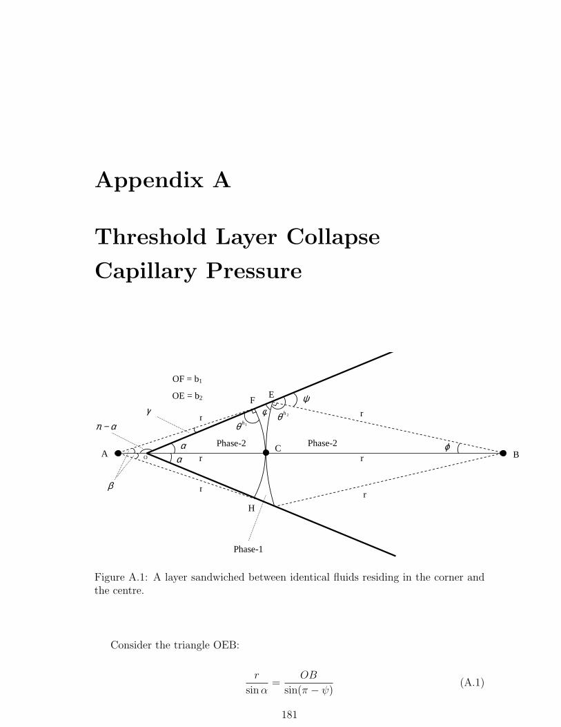
Appendix A
Threshold Layer Collapse
Capillary Pressure
B O
Phase-1
α
α
2hθ
A
r
r
E
C
H
F
απ −
γ
β
Phase-2
φ
ϕ
ψ
Phase-2
r
r
OF = b1
OE = b2
r r
1hθ
Figure A.1: A layer sandwiched between identical fluids residing in the corner andthe centre.
Consider the triangle OEB:
r
sin α=
OB
sin(π − ψ)(A.1)
181
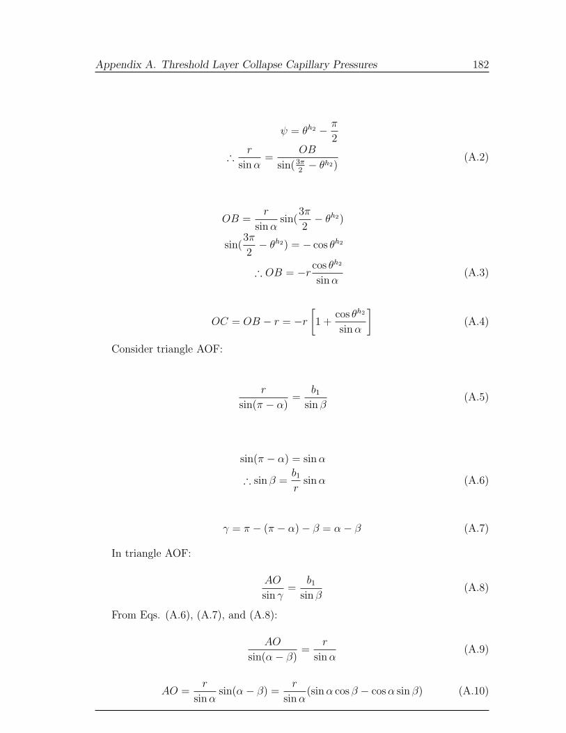
Appendix A. Threshold Layer Collapse Capillary Pressures 182
ψ = θh2 − π
2
∴ r
sin α=
OB
sin(3π2− θh2)
(A.2)
OB =r
sin αsin(
3π
2− θh2)
sin(3π
2− θh2) = − cos θh2
∴ OB = −rcos θh2
sin α(A.3)
OC = OB − r = −r
[1 +
cos θh2
sin α
](A.4)
Consider triangle AOF:
r
sin(π − α)=
b1
sin β(A.5)
sin(π − α) = sin α
∴ sin β =b1
rsin α (A.6)
γ = π − (π − α)− β = α− β (A.7)
In triangle AOF:
AO
sin γ=
b1
sin β(A.8)
From Eqs. (A.6), (A.7), and (A.8):
AO
sin(α− β)=
r
sin α(A.9)
AO =r
sin αsin(α− β) =
r
sin α(sin α cos β − cos α sin β) (A.10)
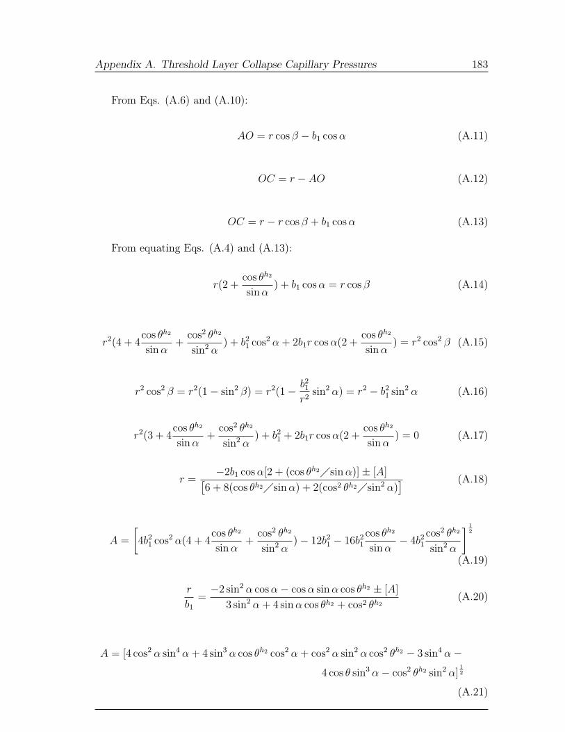
Appendix A. Threshold Layer Collapse Capillary Pressures 183
From Eqs. (A.6) and (A.10):
AO = r cos β − b1 cos α (A.11)
OC = r − AO (A.12)
OC = r − r cos β + b1 cos α (A.13)
From equating Eqs. (A.4) and (A.13):
r(2 +cos θh2
sin α) + b1 cos α = r cos β (A.14)
r2(4 + 4cos θh2
sin α+
cos2 θh2
sin2 α) + b2
1 cos2 α + 2b1r cos α(2 +cos θh2
sin α) = r2 cos2 β (A.15)
r2 cos2 β = r2(1− sin2 β) = r2(1− b21
r2sin2 α) = r2 − b2
1 sin2 α (A.16)
r2(3 + 4cos θh2
sin α+
cos2 θh2
sin2 α) + b2
1 + 2b1r cos α(2 +cos θh2
sin α) = 0 (A.17)
r =−2b1 cos α[2 + (cos θh2�sin α)]± [A][
6 + 8(cos θh2�sin α) + 2(cos2 θh2�sin2 α)] (A.18)
A =
[4b2
1 cos2 α(4 + 4cos θh2
sin α+
cos2 θh2
sin2 α)− 12b2
1 − 16b21
cos θh2
sin α− 4b2
1
cos2 θh2
sin2 α
] 12
(A.19)
r
b1
=−2 sin2 α cos α− cos α sin α cos θh2 ± [A]
3 sin2 α + 4 sin α cos θh2 + cos2 θh2(A.20)
A = [4 cos2 α sin4 α + 4 sin3 α cos θh2 cos2 α + cos2 α sin2 α cos2 θh2 − 3 sin4 α−4 cos θ sin3 α− cos2 θh2 sin2 α]
12
(A.21)
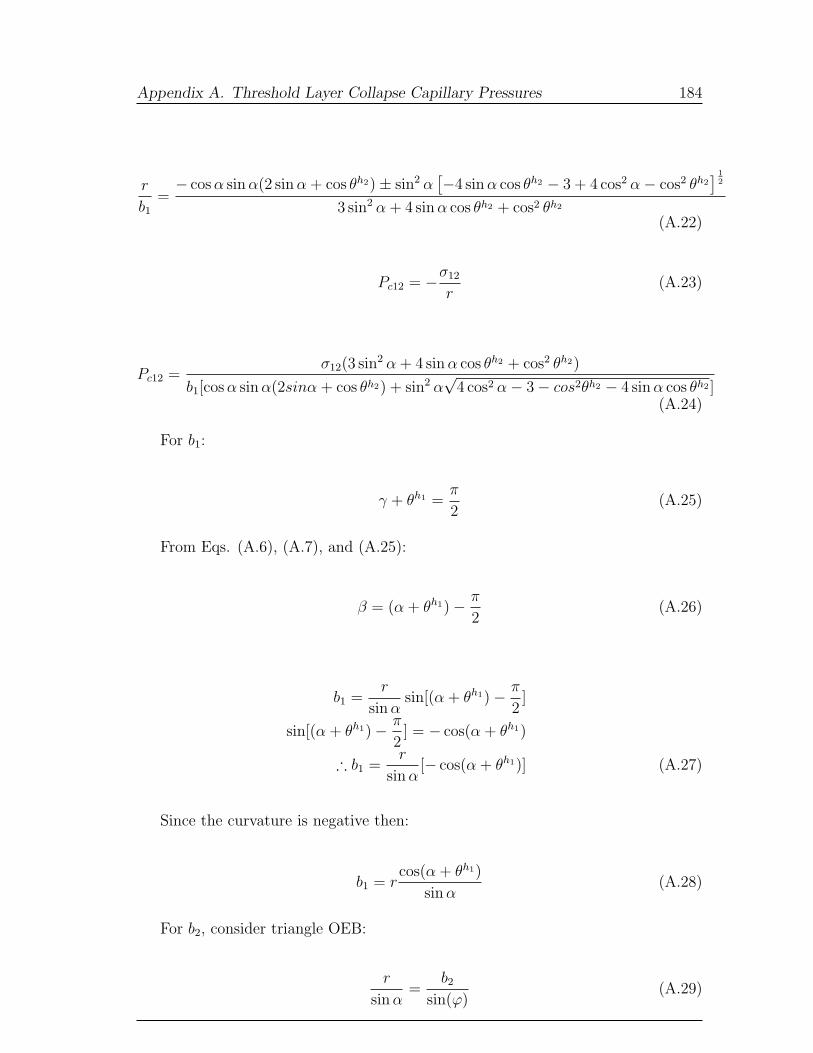
Appendix A. Threshold Layer Collapse Capillary Pressures 184
r
b1
=− cos α sin α(2 sin α + cos θh2)± sin2 α
[−4 sin α cos θh2 − 3 + 4 cos2 α− cos2 θh2] 1
2
3 sin2 α + 4 sin α cos θh2 + cos2 θh2
(A.22)
Pc12 = −σ12
r(A.23)
Pc12 =σ12(3 sin2 α + 4 sin α cos θh2 + cos2 θh2)
b1[cos α sin α(2sinα + cos θh2) + sin2 α√
4 cos2 α− 3− cos2θh2 − 4 sin α cos θh2 ](A.24)
For b1:
γ + θh1 =π
2(A.25)
From Eqs. (A.6), (A.7), and (A.25):
β = (α + θh1)− π
2(A.26)
b1 =r
sin αsin[(α + θh1)− π
2]
sin[(α + θh1)− π
2] = − cos(α + θh1)
∴ b1 =r
sin α[− cos(α + θh1)] (A.27)
Since the curvature is negative then:
b1 = rcos(α + θh1)
sin α(A.28)
For b2, consider triangle OEB:
r
sin α=
b2
sin(ϕ)(A.29)
Appendix B. 185
ϕ = π − (3π
2− θh2)− α
ϕ = −π
2+ θh2 − α
θh2 = π − φ
∴ ϕ =π
2− (α + φ) (A.30)
From Eqs. (A.29) and (A.30):
sin ϕ = sin[π
2− (α + φ)] = cos(α + φ)
∴ b2 = rcos(α + φ)
sin α(A.31)
Appendix B
Parameters in the Model
Input parameters of the model are summarized here. For each item the value(s)/equations(s)
that are used in this work are given within the parentheses.
• Fraction of the clay volume saturated with water to control irreducible water
saturation (1).
• Interfacial tensions to be used in capillary pressure and area calculations (see
Table (7.1)).
• A section of the network where saturations and relative permeabilities are
computed (the central 90% of the network).
• A large positive integer number to be used in random number generation, seed
(12357).
• Maximum number of iterations to be used in pressure solver (30000).
• Convergency criterion to be used in pressure solver (5.0E − 06).
• Pore-body filling model to be used in calculation of threshold capillary pres-
sures for imbibition in pores (Eq. (4.64), see section (4.4.2)).
• Parameters of pore-body filling model (e1 = 0 and e2 − en = 0.03 µm−1, see
section (4.4.2)).
• Contact angles to be used in threshold capillary pressure and area calculations
(see Tables (7.2) and (7.3)).
186