Embed Size (px)
Citation preview
POPULATION MODELS IN ALMOST PERIODICENVIRONMENTS
TOKA DIAGANA, SABER ELAYDI, AND ABDUL-AZIZ YAKUBU
Abstract. We establish the basic theory of almost periodic sequences on Z+.Dichotomy techniques are then utilized to find sufficient conditions for the ex-istence of a globally attracting almost periodic solution of a semilinear systemof difference equations. These existence results are, subsequently, applied todiscretely reproducing populations with and without overlapping generations.Furthermore, we access evidence for attenuance and resonance in almost peri-odically forced population models.
1. Introduction
Despite the fact that all natural populations suffer temporal environmental fluc-tuations on some scale, experimental and theoretical studies of population responsesto external fluctuations remain relatively rare [8, 9, 10], [12, 13, 14, 15, 16, 17],[20, 21, 22, 23, 24], [28, 29, 30], [32], and [35, 36, 36, 38, 39, 40, 41]. To study theeffects of fluctuating environments on population dynamics, one can deliberatelyfluctuate environmental parameters in controlled laboratory experiments. Jillsonperformed such an experiment with laboratory cultures of Tribolium [34]. Othershave used mathematical models to study the effects of periodic forcing on popula-tion dynamics [8, 9, 10], [12, 13, 14, 15, 16, 17], [20, 21, 22, 23, 24], [29, 30], and[35, 36, 37, 38].
Though one can deliberately periodically fluctuate environmental parameters incontrolled laboratory experiments, fluctuations in nature are hardly periodic. Thatis, almost periodicity is more likely to accurately describe natural fluctuations.Almost periodicity has been observed in data collected by Henson et al. on tidalheights [31]. The ecological literature is filled with future life-history studies ofperiodically forced (nonautonomous) classical parametric population models withtime t in Z+. Examples of such periodically forced parametric models with timet in Z+ include the Beverton-Holt, Ricker, Smith-Slatkin and LPA models [9, 10],[13, 14, 15, 16], and [21, 22, 23, 24].
In this paper, we focus on the effects of almost periodic environments on popu-lation dynamics. That is, we study future life-history evolutions in these environ-ments with time t ∈ Z+. For that, we make extensive use of dichotomy techniquesto find sufficient conditions for the existence of a globally attracting almost peri-odic solution to a semilinear system of difference equations. These existence resultsare applied to discretely reproducing populations with and without overlappinggenerations.
2000 Mathematics Subject Classification. 34C27; 34K14; 34D23.Key words and phrases. Bohr almost periodic sequences, Bochner almost periodic sequences,
almost periodicity, regular dichotomy, globally attracting almost periodic solution, Beverton-Holtequation, Beverton-Holt equation with delay.
1
2 TOKA DIAGANA, SABER ELAYDI, AND ABDUL-AZIZ YAKUBU
The paper is organized as follows: in Section 2, we establish the theory of al-most periodic sequences on Z+. In particular, we show that the notions of Bohrand Bochner almost periodic sequences on Z+ are equivalent. In Section 3, we pro-vide a method to construct almost periodic sequences on Z+. Sufficient conditionsfor the existence of a globally attracting almost periodic solution of a semilinearsystem of difference equations are given in Section 4 (Theorem 4.6). In Section 5(respectively, Section 6), we apply Theorem 4.6 to population models with non-overlapping generations (respectively, overlapping generations). Section 7 is onaccessing evidence of attenuance and resonance in almost periodic environments.Extensions to population models with delay are developed in Sections 8 and 9, andthe implications of our results are discussed in Section 10.
2. Preliminaries
In this section, we establish the basic theory of almost periodic sequences on Z+.But first, let us introduce the notation needed in the sequel.
Let (R, | · |), (Rk, | · |), R+, Z, Z+ be the field of real numbers equipped withits absolute value, the k−dimensional space of real numbers equipped with theEuclidean topology, the set of positive real numbers, the set of all integers, and theset of all nonnegative integers, respectively.
Our main objective in this paper is to find sufficient conditions for the existence ofa globally attracting almost periodic solution of the semilinear systems of differenceequations
(2.1) x(t + 1) = A(t)x(t) + f(t, x(t)), t ∈ Z+
where A(t) is a k × k almost periodic matrix function defined on Z+, and thefunction f : Z+ × Rk → Rk is almost periodic.
To study solutions of Eq. (2.1), we use the fundamental solutions of the system
(2.2) x(t + 1) = A(t)x(t), t ∈ Z+,
to examine almost periodic solutions of the system of difference equations
(2.3) x(t + 1) = A(t)x(t) + g(t), t ∈ Z+
where g : Z+ → Rk is almost periodic.
Let l∞(Z+) denote the Banach space of all bounded Rk-valued sequences equippedwith the sup norm defined for each x = {x(t)}t∈Z+
∈ l∞(Z+), by
‖x‖∞ = supt∈Z+
‖x(t)‖ .
Let N(Z+) ⊂ l∞(Z+) denote the subspace of all null sequences.
Definition 2.1. [18, 19, 25, 33, 43, 44] An Rk-valued sequence x = {x(t)}t∈Z+is
called Bohr almost periodic if for each ε > 0, there exists a positive integer T0(ε)such that among any T0(ε) consecutive integers, there exists at least one integer τwith the following property:
‖x(t + τ)− x(t)‖ < ε, ∀t ∈ Z+.
The integer τ is then called an ε-period of the sequence x = {x(t)}t∈Z+.
POPULATION MODELS IN ALMOST PERIODIC ENVIRONMENTS 3
Definition 2.2. [18, 19, 25, 33, 43] An Rk-valuedsequence x = {x(t)}t∈Z+is called
Bochner almost periodic if for every sequence {h(t)}t∈Z+⊂ Z+ there exists a subse-
quence {h(Ks)}s∈Z+such that {x(t + h(Ks))}s∈Z+
converges uniformly in t ∈ Z+.
One should point out that combining the extension theorem [2, Proposition4.7.1, p. 305] (of an almost periodic function on R+ to an almost periodic functionR) and [6, Theorem 1.27, p. 47], it is not hard to see that if {x(t)}t∈Z+ is anRk-valued almost periodic sequence, then there exists a unique almost periodicfunction f : R 7→ Rk such that x(t) = f(t) for each t ∈ Z+. Unlike the case ofalmost periodicity on Z, here, we make use of other techniques to establish ourpreliminary results on almost periodicity on Z+ rather than equations of the formx(t) = f(t), t ∈ Z+.
We use the following result to reconcile the two definitions of almost periodicsequences.
Proposition 2.3. Let xm = {xm(t)}t∈Z+be a Bohr almost periodic sequence con-
verging uniformly in m ∈ Z+ to x, then the sequence x is Bohr almost periodic.
Proof. The proof is similar to the one in Halanay [25, Proposition 4.7, p. 229] forsequences in Z and hence omitted. ¤
The next step consists of showing that the two definitions of almost periodicsequences in Z+ are equivalent.
Theorem 2.4. A sequence x = {x(t)}t∈Z+is Bochner almost periodic if and only
if it is Bohr almost periodic.
Proof. First, we show that if x = {x(t)}t∈Z+is Bochner almost periodic, then it is
Bohr almost periodic. To achieve this, we show that if x = {x(t)}t∈Z+is not Bohr
almost periodic, then it is not Bochner almost periodic.Suppose that x = {x(t)}t∈Z+
is not Bohr almost periodic. Then there exists atleast one ε > 0 such that for any positive integer T0, there exist T0 consecutivepositive integers which contain no ε-period related to the sequence {x(t)}t∈Z+
. Now,let h(1) ∈ Z+ and let 2α1 +1, 2α1 +2, 2α1 +3, ..., 2β1−2, 2β1−1 be (2β1−2α1−1)-positive integers (α1, β1 ∈ Z+) such that 2β1−2α1−2 > 2h(1) or β1−α1−1 > h(1)and the sequence 2α1 + 1, 2α1 + 2, 2α1 + 3, ..., 2β1− 2, 2β1− 1 does not contain anyε-period related to {x(t)}t∈Z+
.Next, let h(2) = 1
2 (2α1 + 2β1) = α1 + β1. Clearly, h(2) − h(1) is a (positive)integer such that 2α1 + 1 < h(2) − h(1) < 2β1 − 1, and hence h(2) − h(1) cannotbe an ε-period. Thus, there exist 2α2 + 1, 2α2 + 2, 2α2 + 3, ..., 2β2 − 2, 2β2− 1 suchthat 2β2 − 2α2 − 2 > 2(h(1) + h(2)), which does not contain any ε-period relatedto {x(t)}t∈Z+
. Setting h(3) = 12 (2α2 + 2β2) = α2 + β2, it follows that h(3)− h(2),
h(3) − h(1) are respectively one of the terms 2α2 + 1, 2α2 + 2, 2α2 + 3, ..., 2β2 −2, 2β2−1, and hence h(3)−h(2), h(3)−h(1) are not ε-period related to {x(t)}t∈Z+
.Proceeding as previously, one defines the numbers h(4), h(5), ..., such that none ofthe expressions h(i)− h(j) for i > j is an ε-period for the sequence {x(t)}t∈Z+
.
4 TOKA DIAGANA, SABER ELAYDI, AND ABDUL-AZIZ YAKUBU
Consequently, for all i, j ∈ Z+,
supi,j‖x(t + h(i))− x(t + h(j))‖ ≥ sup
i>j‖x(t + h(i))− x(t + h(j))‖
= supi>j
‖x(t + h(i)− h(j))− x(t)‖≥ ε.
This proves that {x(t + h(i))}i∈Z+cannot contain any uniformly convergent se-
quence, and hence {x(t)}t∈Z+is not Bochner almost periodic.
Conversely, suppose that the sequence {x(t)}t∈Z+is Bohr almost periodic and
{tj}j∈Z+is a sequence of positive integers. Here, we adapt our proof to the one
given in [25, Proof of Theorem 4.9., p. 230-231]. For each ε > 0 there exists aninteger T0 > 0 such that between tj and T0 + tj there exist an ε-period τj with0 ≤ τj − tj ≤ T0. Setting sj = τj − tj , one can see that sj can take only a finitenumber (at most T0 + 1) values, and hence there is some s, 0 ≤ s ≤ T0 such thatsj = s for an infinite numbers of j′s. Let these indexes be numbered as jk, then wehave
‖x(t + tj)− x(t + sj)‖ = ‖x(t + τj + sj)− x(t + sj)‖ < ε.
Hence,‖x(t + tj)− x(t + sj)‖ < ε
for all t ∈ Z+.One may complete the proof by proceeding exactly as in [25, Proof of Theorem
4.9., pp. 230-231] and using [25, Proposition 4.7] relative to Z+ rather than Z.
Now let {εr}r∈Z+be a sequence such that ε → 0 as r →∞, say εr =
1r + 1
. Now,
from the sequence {x(n + tj)}j∈Z+, consider a subsequence chosen so that
∥∥∥x(n + tj1i)− x(n + s1)
∥∥∥ ≤ ε1.
Next, from the previous sequence, we take a new subsequence such that∥∥∥x(n + tj2i)− x(n + s2)
∥∥∥ ≤ ε2.
Repeating this procedure and for each r ∈ Z+ we obtain a subsequence{x(n + tjr
i)}
i∈Z+
such that ∥∥x(n + tjri)− x(n + sr)
∥∥ ≤ εr.
Now, for the diagonal sequence,{
x(n + tjii)}
i∈Z+
, for each ε > 0 take k(ε) ∈ Z+
such that εk(ε) < ε2 , where εr belongs to the previous sequence {εr}r∈Z+
.
Using the fact that the sequences{tjr
r
}and
{tjs
s
}are both subsequences of{
tj
k(ε)i
}, for r ≥ k(ε) we have
∥∥x(n + tjrr)− x(n + tjs
s)∥∥ ≤ ∥∥x(n + tjr
r)− x(n + sk)
∥∥+
∥∥x(n + sk)− x(n + tjss)∥∥
≤ εk(ε) + εk(ε)
≤ ε.
Thus, the sequence{
x(n + tjii)}
i∈Z+
is a Cauchy sequence.
¤
POPULATION MODELS IN ALMOST PERIODIC ENVIRONMENTS 5
Let x = {x(i)}i∈Z+and α = {α(j)}j∈Z+
be Rk-valued sequences. Define
Tαx := {y = (yj)j∈Z+ : y(j) = limi→∞
x(j + α(i))}.Theorem 2.5. Let x be a sequence. Suppose that for every pair α′, β′ of sequencesin Z+ there exist common subsequences α, β where α is a subsequence of α′ and βthat of β′, such that TαTβx = Tα+βx pointwise in Z+. Then x is almost periodic.
The proof of Theorem 2.5 is similar to the one given for sequences in Z [25,Theorem 4.18, pp 234-235], and is omitted.
The collection of all almost periodic Rk-valued sequences on Z+ will be denotedby AP (Z+). It is a Banach space when equipped with the sup norm defined above.
Lemma 2.6. If {x(t)}t∈Z+is almost periodic, then it is bounded.
Proof. Assume that {x(t)}t∈Z+is not bounded. Then for some subsequence
‖x(ti)‖ → ∞ as i →∞.
Let ε = 1. Then there exists T (ε) ∈ Z+ − {0} that satisfies the almost periodicitydefinition. There exists ti = s1 such that ti = s1 > T (ε). Then among the integers
{s1 − T (ε) + 1, s1 − T (ε) + 2, ..., s1}there exists s1 such that
‖x(t + s1)− x(t)‖ < 1.
Next, choose tj = s2 such that tj = s2 > T (ε) + s1. Then among the integers
{s2 − T (ε) + 1, s2 − T (ε) + 2, ..., s2}there exists s2 such that
‖x(t + s2)− x(t)‖ < 1.
Repeating this process, we obtain a sequence {si} → ∞ as i →∞ such that
‖x(t + si)− x(t)‖ < 1 for r = 1, 2, 3, ...,
and a subsequence {si} of {ti} with {si} → ∞ as i →∞. Moreover,
si = si + ui
where 0 ≤ ui < T (ε).Since {ui} is finite, there exists ui0 that is repeated infinitely many times and
sir = sir + ui0 , where ir →∞ as i →∞. Therefore,
‖x(t + sir )− x(ui0)‖ < 1.
Moreover,‖x(t + sir )− x(ui0)‖ < 1.
Hence, {x(sir )} is bounded; a contradiction.¤
Definition 2.7. A real-valued sequence x = {x(t)}t∈Z+is said to be asymptotically
almost periodic if it can be decomposed as
x(t) = u(t) + υ(t),
where u = {u(t)}t∈Z+∈ AP (Z+) and {υ(t)}t∈Z+
∈ N(Z+).The collection of all asymptotically almost periodic Rk-valued sequences will be
denoted by AAP (Z+).
6 TOKA DIAGANA, SABER ELAYDI, AND ABDUL-AZIZ YAKUBU
Definitions 2.1, 2.2 and 2.7 are respectively adapted from the definitions of Rk-valued almost periodic sequences and asymptotically almost periodic sequencesx = {x(t)}t∈Z defined in Z.
Lemma 2.8. If x = {x(t)}t∈Z+∈ AP (Z+) and lim
t→∞x(t) = 0, then x(t) = 0 for all
t ∈ Z+.
Proof. Let εt =1
t + 1for each t ∈ {0, 1, ...}. Then there exists T (εt) such that
among t, t + 1, ..., t + T (εt)− 1, there exists st such that
‖x(t + st)− x(t)‖ ≤ εt for all t ∈ Z+.
As t → ∞, st → ∞, x(t + st) → 0, and εt → 0. Hence, ‖x(t)‖ ≤ 0. This impliesthat x(t) = 0 for all t ∈ Z+.
¤
Lemma 2.9. The decomposition of an asymptotically almost periodic sequence isunique. That is, AP (Z+)∩ N(Z+) = {0}.Proof. Suppose that x = {x(t)}t∈Z+
can be decomposed as
x(t) = u(t) + υ(t)
andx(t) = v(t) + δ(t),
where u = {u(t)}t∈Z+, ν = {ν(t)}t∈Z+
∈ AP (Z+) and {υ(t)}t∈Z+, {δ(t)}t∈Z+
∈N(Z+). Clearly, u(t) − ν(t) = δ(t) − υ(t) ∈ AP (Z+)∩ N(Z+). By Lemma 2.8,u(t) = ν(t) and υ(t) = δ(t) for all t ∈ Z+.
¤
Theorem 2.10. Assume that (t, w) 7→ f(t, w) is Lipschitz in w uniformly in t ∈Z+. If x(t) = u(t)+υ(t) is a solution of Eq. (2.1), then {u(t)}t∈Z+
is also a solutionof Eq. (2.1), where u = {u(t)}t∈Z+
∈ AP (Z+) and ν = {ν(t)}t∈Z+∈ N(Z+).
Proof. Let {x(t)}t∈Z+be an asymptotically almost periodic solution of Eq. (2.1).
That is, x(t) = u(t) + υ(t), where {u(t)}t∈Z+∈ AP (Z+) and {υ(t)}t∈Z+
∈ N(Z+).Now
u(t + 1)−A(t)u(t)− f(t, u(t)) = x(t + 1)− υ(t + 1)−A(t)u(t)− f(t, u(t))= A(t)x(t) + f(t, x(t))− υ(t + 1)− A(t)u(t)− f(t, u(t)).
Consequently,
‖u(t + 1)−A(t)u(t)− f(t, u(t))‖≤ (L + ‖A(t)‖) · ‖x(t)− u(t))‖+ ‖υ(t + 1)‖
≤(
L + supt∈Z+
‖A(t)‖)· ‖υ(t))‖+ ‖υ(t + 1)‖ .
Hence, ‖u(t + 1)−A(t)u(t)− f(t, u(t))‖ → 0 as t →∞.
POPULATION MODELS IN ALMOST PERIODIC ENVIRONMENTS 7
Let w(t) = u(t + 1) − A(t)u(t) − f(t, u(t)). If w(T ) 6= 0 for some t ∈ Z+, let
ε =|w(T )|
2> 0. Thus,
|w(T + p)− w(T )| ≤ |w(T )|2
.
Hence,
|w(T + p)| ≥ |w(T )|2
.
Let It = [sl, (s + 1) l] be intervals of length l. For each interval Is there exists ps
such that |w(T + ps)| ≥ |w(T )|2
. As s →∞, ps →∞, and
limt→∞
|w(t)| ≥ |w(T )|2
> 0.
This contradicts the fact that limt→∞ |w(t)| = 0. Therefore, w(t) = 0 for eacht ∈ Z+. That is, u(t + 1) = A(t)u(t) + f(t, u(t)) where {u(t)}t∈Z+
is almostperiodic.
¤
Definition 2.11. A sequence F : Z+ × Rp 7→ Rq, (t, u) 7→ F (t, u) is called almostperiodic in t ∈ Z+ uniformly in u ∈ Rq if for each ε > 0 there exists a positiveinteger T0(ε) such that among any T0(ε) consecutive integers, there exists at leastone integer s with the following property:
‖F (t + s, u)− F (t, u)‖ < ε
for all u ∈ Rq and t ∈ Z+.
Theorem 2.12. Suppose that F : Z+×Rp → Rq, (t, u) 7→ F (t, u) is almost periodicin t ∈ Z+ uniformly in u ∈ Rp. If in addition, F is Lipschitz in u ∈ Rp uniformlyin t ∈ Z+ (that is, there exists L > 0 such that
‖F (t, u)− F (t, v)‖ ≤ L ‖u− v‖ ∀u, v ∈ Rp, t ∈ Z+),
then for every Rp-valued almost periodic sequence x = {x(t)}t∈Z+ , the Rq-valuedsequence y(t) = F (t, x(t)) is almost periodic.
Proof. Let x = {x(t)}t∈Z+be an almost periodic sequence and let y(t) = F (t, x(t)).
Then, for each ε > 0 there exists a positive integer T0(ε) such that among any T0(ε)consecutive integers, there exists at least one integer s with the following property:
‖x(t + s)− x(t)‖ <ε
L∀ t ∈ Z+.
Moreover,
‖y(t + s)− y(t)‖ = ‖F (t + s, x(t + s))− F (t, x(t))‖≤ ‖F (t + s, x(t + s))− F (t + s, x(t))‖
+ ‖F (t + s, x(t))− F (t, x(t))‖≤ L ‖x(t + s)− x(t))‖+
ε
2<
ε
2+
ε
2= ε.
¤
8 TOKA DIAGANA, SABER ELAYDI, AND ABDUL-AZIZ YAKUBU
3. Construction of Almost Periodic Sequences on Z+
There are two ways of generating an almost periodic sequence on Z+. One maystart with a periodic function on R or an almost periodic function on R. In thesequel we will describe these two approaches.
(i) Periodic Functions. Let f : R→ Rk be a periodic function with periodic ω.
(a) If ω is a rational number, ω =r
s, r, s ∈ Z+ with s 6= 0, then r = sω is also
a period of f . If we let x(t) = f(t), t ∈ Z, then (x(t))t∈Z+ is a periodicsequence of period r.
(b) Now assume that ω is an irrational number. Then f is uniformly continuousand hence, given ε > 0, there exists δ > 0 such that |x− y| < δ implies
‖f(x)− f(y)‖ < ε.(3.1)
There exists a rational numberr
ssuch that |ω − r
s| < δ
sand consequently,
|sω − r| < δ.(3.2)
Define x(t) = f(t), t ∈ Z. Then
‖x(t + r)− x(t)‖ ≤ ‖f(t + r)− f(t + sω)‖+ ‖f(t + sω)− f(t)‖< ε,
by Eq. (3.1).(ii) Almost Periodic Functions. This case can also be divided into two cases. Let
f : R 7→ Rk be an almost periodic function,and ε > 0 be given. Then there existsT (ε) such that for any interval of length T (ε), there exists a number ω with
‖f(t + ω)− f(t)‖ < ε for all t ∈ R.
(a) If ω =r
sis rational, then we consider T (ε) = sT (ε), ω = sω. If we let
x(t) = f(t), t ∈ Z, it follows that T (ε) and ω are the integers needed tomake x(t) almost periodic on Z and
‖f(t + ω)− f(t)‖ <ε
2s.(3.3)
(b) Now assume that ω is irrational. Since f is uniformly continuous, givenε > 0, there exists δ > 0 such that |x− y| < δ implies ‖f(x) − f(y)‖ <
ε
2.
There exists a rational numberr
s, r, s ∈ Z+ with s 6= 0 such that |r
s−ω| <
δ
s. Hence |r − sω| < δ and consequently,
‖f(t + r)− f(t + sω)‖ <ε
2, for all t ∈ R.(3.4)
Define x(t) = f(t), t ∈ Z. Then
‖x(t + r)− x(t)‖ ≤ ‖f(t + r)− f(t + sω)‖+ ‖f(t + sω)− f(t)‖<
ε
2,
POPULATION MODELS IN ALMOST PERIODIC ENVIRONMENTS 9
by Eq. (3.3) and Eq. (3.4).Let T (ε) = bsωc + 1 (b·c being the greatest integer function). Then r
and T (ε) provide with the almost periodicity of (x(t))t∈Z.I. Finally, once we get an almost periodic sequence {x(t)}t∈Z, we define an asso-
ciated sequence {x(t)}, where x(t) = x(t)u0(t) (u0 being the Heaviside function).The sequence {x(t)} is almost periodic on Z+ but not on Z.
II. (a) An example for case (i) is the function f(t) = cos(αt) with period ω =2π
α.
Then x(t) = cos(αt)u0(t) is almost periodic on Z+.
(b) For case (ii), we let f(t) = cos(αt) + cos(βt) with2πα
or2π
βis irrational.
Then x(t) = (cos(αt) + sin(βt)) u0(t) is almost periodic on Z+ but not on Z.
Remark 3.1. (i) Since almost periodic functions f on R can be approximated bytrigonometric polynomials, it follows that almost periodic sequences x(t) on Z+
that are constructed in the manner described above can also be approximated bytrigonometric sequences.
(ii) Almost periodic sequences may be generated as solutions of scalar differenceequations or systems of difference equations. The following examples elucidate thispoint.
Example 3.2. Consider the second-order difference equation
x(t + 2)− 2 cos αu0(t)x(t + 1) + x(t) = 0, x(0) = 0, x(1) = 1,
where 0 < α < π and α is not a multiple of π. Then the solution is given by
x(t) =
sin(tα)sin α
if t ≥ 0
...x(−4), x(−3), x(−2), x(−1) if t < 0
where x(−1) = −1, x(−2) = 0, x(−3) = 1, x(−4) = 0, and this is of period 4.Clearly, {x(t)} is almost periodic on Z+ but not on Z.
Example 3.3. This set of examples is inspired by Corduneanu [6, Theorem 8]. Con-sider the k-dimensional system of difference equations
x(t + 1) = Ax(t) + g(t)
where A is a k × k-matrix and g is assumed to be almost periodic on Z. Then by[6, Theorem 8], any bounded solution of the previous system is necessarily almostperiodic on Z. And by the construction above this produces an almost periodicsequence on Z+.
4. Regular Exponential Dichotomy
In Eq. (2.2), the classical definition of dichotomy does not apply, whenever thestate transition matrix
X(t, s) =t−1∏r=s
A(r)
is not invertible. In [27], Henry used the following definition to address this problem.
10 TOKA DIAGANA, SABER ELAYDI, AND ABDUL-AZIZ YAKUBU
Definition 4.1. Eq. (2.2) is said to have a regular exponential dichotomy if thereexists k × k projection matrices P (t) with t ∈ Z+ and positive constants M andβ ∈ (0, 1) such that the following four conditions are satisfied:
(i) A(t)P (t) = P (t + 1)A(t);(ii) The matrix A(t) |R(I−P (t)) is an isomorphism from R(I−P (t)) onto R(I−
P (t + 1));(iii) ‖X(t, r)P (r)x‖ ≤ Mβt−r ‖x‖ , for 0 ≤ r ≤ t, x ∈ Rk;(iv) ‖X(r, t)(I − P (t))x‖ ≤ Mβt−r ‖x‖ , for 0 ≤ r ≤ t, x ∈ Rk.
By repeated application of [(i), Definition 4.1], we obtain
(4.1) P (t)X(t, s) = X(t, s)P (s).
Define the hull H(x) of a sequence x as follows:
Definition 4.2. The set
H(x) = {x | there exists a sequence α in Z+ with Tαx = x}.Similarly, for a matrix function A(t), we define
H(A) = {A | there exists a sequence α in Z+ with TαA = A},where TαA = A means that lim
t→∞A(t + α(t)) = A(t).
Theorem 4.3. Suppose that Eq. (2.2) has a regular exponential dichotomy andA(t) ∈ H(A(t)). Then the system
x(t + 1) = A(t)x(t)
satisfies a regular exponential dichotomy with same projections and constants.
Proof. Let TαA = A. Then Xi(t) = X(t + αi) is a fundamental matrix for theequation
x(t + 1) = A(t + αi)x(t)
and satisfies regular exponential dichotomy with the same projection P (i) and sameconstants M and β.
One may take subsequences so that Xi(0) converges to Y0. For a suitable sub-sequence, Xi(t) converges to a solution Y (t) of
x(t + 1) = A(t)x(t).
Then Y (0) = Y0 and Y (t) satisfies the conditions of regular exponential dichotomy.¤
Theorem 4.4. Suppose that Eq. (2.2) has a regular exponential dichotomy andA(t) ∈ H(A(t)). Then, Eq. (2.3) has an almost periodic solution given by
(4.2) x(t) =t−1∑
r=−∞X(t, r + 1)P (r + 1)g(r)−
∞∑r=t
X(t, r + 1)(I − P (r + 1))g(r),
where X(t, r)P (r) = 0 for r > t and g(r) = 0 for r < 0.
POPULATION MODELS IN ALMOST PERIODIC ENVIRONMENTS 11
Proof. It can be easily verified that x(t) defined by Eq. (4.2) is indeed a solutionof Eq. (2.3). Moreover,
‖x(t)‖ ≤{
t−1∑r=−∞
‖X(t, r + 1)P (r + 1)‖+∞∑
r=t
‖X(t, r + 1)(I − P (r + 1))‖}‖g‖
≤{
t−1∑r=0
Mβt−r−1 +∞∑
r=t
Mβr+1−t
}‖g‖ ≤ M
1 + β
1− β‖g‖ .
Let {α} and {γ} be arbitrary sequences of nonnegative integers, and let {α} ⊂{α} and {γ} ⊂ {γ} be their common subsequences. Then Tα+γA = TγTαA andTα+γg = TγTαg. Now,
x(t + αi) =t+αi−1∑r=−∞
X(t + αi, r + 1)P (r + 1)g(r)−
∞∑r=t+αi
X(t + αi, r + 1)(I − P (r + 1))g(r)
=t−1∑
s=−∞X(t + αi, s + αi + 1)P (s + αi + 1)g(s + αi)−
∞∑s=t
X(t + αi, s + αi + 1)(I − P (s + αi + 1))g(s + αi)
=t−1∑
s=−∞A(t + αi − 1) · · ·A(s + αi + 1)P (s + αi + 1)g(s + αi)−
∞∑s=t
A(t + αi − 1) · · ·A(s + αi + 1)(I − P (s + αi + 1))g(s + αi).
limi→∞
x(t + αi) = (Tαx)t =t−1∑
s=−∞A(t− 1) · · · A(s + 1)P (s + 1)g(s)−
∞∑s=t
A(t− 1) · · · A(s + 1)(I − P (s + 1))g(s)
=t−1∑
s=−∞(TαA)t−1 · · · (TαA)s+1 (TαP )s+1 (Tαg)s −
∞∑s=t
(TαA)t−1 · · · (TαA)s+1 (I − TαP )s+1 (Tαg)s .
Moreover,
(TγTαx)t =t−1∑
s=−∞(TγTαA)t−1 · · · (TγTαA)s+1 (TγTαP )s+1 (TγTαg)s −
t−1∑s=t
(TγTαA)t−1 · · · (TγTαA)s+1 (I − TγTαP )s+1 (TγTαg)s
= (Tγ+αx)t .
12 TOKA DIAGANA, SABER ELAYDI, AND ABDUL-AZIZ YAKUBU
Hence, {x(t)}t∈Z+∈ AP (Z+).
¤
Corollary 4.5. If the zero solution of Eq. (2.2) is uniformly asymptotically stable,then Eq. (2.3) has a unique globally asymptotically stable almost periodic solution,
x(t) =t−1∑r=0
(t−1∏s=r
A(s)
)g(r).
Moreover,
‖x(t)‖ ≤ Mβ
1− β‖g‖ .
Proof. Let y(t) be a solution of Eq. (2.3) with y(0) = y0. Then,
y(t) = X(t)y0 +t−1∑r=0
(t−1∏s=r
A(s)
)g(r).
Therefore,y(t) = γ(t) + x(t),
where γ(t) is a null sequence. Thus, y(t) is an asymptotically almost periodicsolution of Eq. (2.3). By Lemma 2.9, y(t) ∈ AP (Z+) implies that y = x. Hence,
x(t) =t−1∑r=0
(t−1∏s=r
A(s)
)g(r)
is the only almost periodic solution of Eq. (2.3).
It is easy to see that ‖x(t)‖ ≤ Mβ
1− β‖g‖.
Theorem 4.6. Suppose that f is Lipschitz with Lipschitz constant L. Then Eq. (2.1)has a unique globally asymptotically stable almost periodic solution if
(4.3)MβL
1− β< 1.
Proof. Consider the Banach space AP (Z+) equipped with the sup norm. By The-orem 2.12, if ϕ ∈ AP (Z+) then f(t, ϕ(t)) ∈ AP (Z+). Let
Γ : AP (Z+) → AP (Z+)
be the nonlinear operator defined by
(Γϕ) (t) :=t−1∑r=0
(t−1∏s=r
A(s)
)f(r, ϕ(r)).
By Theorem 4.4, Γ is well defined. Moreover, for ϕ,ψ ∈ AP (Z+),
‖(Γϕ) (t)− (Γψ) (t)‖ ≤ Mβ
1− β‖f(t, ϕ(t))− f(t, ψ(t))‖ ,
and
‖Γϕ− Γψ‖∞ ≤ MβL
1− β‖ϕ− ψ‖∞ .
POPULATION MODELS IN ALMOST PERIODIC ENVIRONMENTS 13
Γ is a contraction wheneverMβL
1− β< 1. Using the Banach fixed point theorem, we
obtain that Γ has a unique fixed point, x. Moreover, x is the globally asymptoticallystable almost periodic solution of Eq. (2.1). ¤
5. Population Models With Non-overlapping Generations
In some plant populations, growth is a discrete process and generations do notoverlap. To study the impact of periodic environments on the long-term populationdynamics of such populations, various researchers have used simple models of thegeneral form
(5.1) x(t + 1) = f(t, x(t)), t ∈ Z+.
where x(t) is the population size at generation t [13-16, 20-23]. The smooth mapf : Z+ × [0,∞) → (0,∞) is the per capita growth rate.
In periodic environments, f is periodic with period p. That is, there exists asmallest positive integer p satisfying f(t + p, x) = f(t, x).
The periodic Beverton-Holt model,
(5.2) x(t + 1) =µKtx(t)
Kt + (µ− 1)x(t),
where the constant intrinsic growth rate µ > 1 and the carrying capacity Kt isperiodic with minimal period p ≥ 2,
Kt+p = Kt > 0,
is an example of Eq. (5.2) in periodic environments.Eq. (2.1) with the linear part, A(t)x(t), missing reduces to Eq. (5.1). In this
case, one may contemplate the variational system
y(t + 1) = B(t)y(t) + g(t, y(t)), t ∈ Z+
where
B(t) =∂
∂xf(t, z(t)),
for some solution z(t) of Eq. (5.1), and
g(t, y(t)) = f(t, y(t))−B(t)y(t).
However, this approach has at least two basic problems. The first problem is that,it is difficult to find the solution z(t) of Eq. (5.1). The second problem is that, thelinear part of Eq. (5)) does not satisfy the hypotheses of Theorem 4.6.
To illustrate the difficulties in a specific example, we consider the almost period-ically forced Beverton-Holt model. That is, in Eq. (5.2) we assume that {Kt}t∈Z+
is almost periodic in Z+ and µ > 1. The variational equation around z(t) = 0associated with Eq. (5.2) is given by
x(t + 1) = µx(t)− µ(µ− 1) (x(t))2
Kt + (µ− 1)x(t).
However, µ > 1 implies that Theorem 4.6 does not apply.A simple substitution transforms Eq. (5.2) into a linear equation. To be more
specific,
y(t) =1
x(t)
14 TOKA DIAGANA, SABER ELAYDI, AND ABDUL-AZIZ YAKUBU
in Eq. (5.2) yields
(5.3) y(t + 1) =1µ
y(t) +µ− 1µKt
, t ∈ Z+
Since Kt ∈ AP (Z+), we have µ−1µKt
∈ AP (Z+). Hence, Corollary 4.5 applies and
Eq. (5.3) has a unique globally asymptotically stable almost periodic solution y(t).Consequently,
x(t) =1
y(t)is the unique almost periodic solution of Eq. (5.2), where Kt ∈ AP (Z+) and µ > 1.Moreover, for any solution x(t) of Eq. (5.2) we have
∣∣∣x(t)− x(t)∣∣∣ =
∣∣∣∣∣1
y(t)− 1
y(t)
∣∣∣∣∣ =
∣∣∣y(t)− y(t)∣∣∣
∣∣∣y(t)y(t)∣∣∣
.
So both y(t) and y(t) are bounded away from zero. As a result,∣∣∣x(t)− x(t)
∣∣∣ ≤ M∣∣∣y(t)− y(t)
∣∣∣ .
Hence, x(t) is globally asymptotically stable. This result was obtained in [32] underthe assumption that the sequence { Kt} is defined for all t ∈ Z+.
6. Population Models With Overlapping Generations
In constant environments, theoretical discrete-time population models are usu-ally formulated under the assumption that the dynamics of the total populationsize in generation t, denoted by x(t), are governed by equations of the form
(6.1) x(t + 1) = f(x(t)) + γx(t),
where γ ∈ (0, 1) is the constant “probability” of surviving per generation, andf : R+ → R+ models the birth or recruitment process [23].
Almost periodic effects can be introduced into Eq. (6.1) by writing the recruit-ment function or the survival probability as almost periodic sequences. This ismodeled with the equation
(6.2) x(t + 1) = f(t, x(t)) + γtx(t),
where either {γt}t∈Z+or f(t, x(t)) ∈ AP (Z+) and each γt ∈ (0, 1).
In a recent paper, Franke and Yakubu, in [23], studied Eq. (6.2) with the periodicconstant recruitment function
(6.3) f(t, x(t)) = Kt(1− γt),
and with the periodic Beverton-Holt recruitment function
(6.4) f(t, x(t)) =(1− γt)µKtx(t)
(1− γt)Kt + (µ− 1 + γt)x(t),
where the carrying capacity Kt is p − periodic, Kt+p = Kt for all t ∈ Z+ andµ > 1 [10, 23]. Franke and Yakubu proved that, the periodically forced recruitmentfunctions Eq. (6.3) and Eq. (6.4) generate globally attracting cycles in Eq. (6.2),see [23]. Here, we use Theorem 4.3 to show that when both {Kt}t∈Z+
and {γt}t∈Z+
POPULATION MODELS IN ALMOST PERIODIC ENVIRONMENTS 15
are almost periodic, then Eq. (6.2) supports a unique globally asymptotically sta-ble almost periodic solution whenever the recruitment function is either Eq. (6.3)(almost periodic constant) or Eq. (6.4) (Almost periodic Beverton-Holt’s model).
Theorem 6.1. Let
f(t, x(t)) =(1− γt)µKtx(t)
(1− γt)Kt + (µ− 1 + γt)x(t),
where both {Kt}t∈Z+and {γt}t∈Z+
are almost periodic, each γt ∈ (0, 1), Kt > 0 andµ > 1. Then Eq. (6.2) has a unique globally asymptotically stable almost periodicsolution whenever
sup{γt |t∈Z+
}<
1µ + 1
.
Proof. Eq. (6.2) is in the form of Eq. (2.1), where
A(t) = γt,
and
f(t, x(t)) =(1− γt)µKtx(t)
(1− γt)Kt + (µ− 1 + γt)x(t).
Consequently,
|f(t, x)− f(t, y)| ≤ (1− γt)2µKt2 |x− y|(1− γt)2K2
t + (µ− 1 + γt)(1− γt)Kt(x + y) + (µ− 1 + γt)2xy
≤ µ |x− y| .Hence, f is Lipschitz with the Lipschitz constant L = µ. Let M = 1 and
β = sup{γt |t∈Z+
}. Then, sup
{γt |t∈Z+
}<
1µ + 1
implies that
MβL
1− β=
µ . sup{γt |t∈Z+
}
1− sup{γt |t∈Z+
} < 1
and Eq. (4.3), is satisfied. Applying Theorem 4.6 yields the result.¤
Proceeding exactly as in the proof of Theorem 6.1, it is easy to see that, whenf(t, x(t)) = Kt(1− γt), then f(t, x)− f(t, y) = 0 and the following result is imme-diate.
Corollary 6.2. Let f(t, x(t)) = Kt(1 − γt), where both {Kt}t∈Z+and {γt}t∈Z+
are almost periodic, each γt ∈ (0, 1) and Kt > 0. Then Eq. (6.2) has a uniqueglobally asymptotically stable almost periodic solution whenever
sup{γt |t∈Z+
}< 1.
7. Attenuance and Resonant Cycles in Almost PeriodicEnvironments
Periodic environments usually diminish (respectively, enhance) populations viaattenuant (respectively, resonant) stable cycles [7, 8, 9, 10], [13, 14, 15, 16], and[21, 22, 23, 24]. In this section, we focus on using precise mathematical definitions ofattenuance and resonance to access evidence for attenuance or resonance in almostperiodic environments. In particular, we prove that Model, Eq. (6.2), supports
16 TOKA DIAGANA, SABER ELAYDI, AND ABDUL-AZIZ YAKUBU
attenuant cycles when the recruitment function is the almost periodically forcedBeverton-Holt model and the survival probability is constant (non-almost periodic).
To be precise, define
M(at) = limi→∞
[at+1 + ... + at+i
i
]
as the mean value of an almost periodic sequence {at} on Z+. (see [25] for a similarproof for almost periodic sequence {at} on Z.) M(at) is then called the mean valueof {at}.Lemma 7.1. Let {xt} be an almost periodic scalar sequence on Z+. Then M(xt)exists.
Proof. The proof is similar to the proof of Theorem 5, p. 690 in Kay Fan [18] andwill be omitted.
Remark 7.2. The above proof of Lemma 7.1 can be extended to Rn or Banachspaces.
In Eq. (6.2), let
f(t, x(t)) =(1− γt)µKtx(t)
(1− γt)Kt + (µ− 1 + γt)x(t),
where {Kt}t∈Z+and {γt}t∈Z+
are almost periodic, and each γt ∈ (0, 1), Kt > 0 andµ > 1. By Corollary 6.2, Eq. (6.2) has a globally asymptotically almost periodicsolution {x(t)} whenever sup
{γt |t∈Z+
}< 1
µ+1 .
Open Problem: Under what conditions do we have
(7.1) M(x(t)) < M(Kt)? (attenuance)
(7.2) M(x(t)) > M(Kt)? (resonance)
Theorem 7.3. . In Eq. (6.2), let
f(t, x(t)) =(1− γt)µKtx(t)
(1− γt)Kt + (µ− 1 + γt)x(t),
where {Kt}t∈Z+is almost periodic, and each γt = γ ∈ (0, 1), Kt > 0 and µ > 1.
Then,(1) M(Kt) ≤ sup
{Kt |t∈Z+
}< ∞;
(2) limt→∞
sup1t
t−1∑t=0
x(t) ≤ limt→∞
sup1t
t−1∑t=0
Kt;
for any solution x(t). If x(t) is the unique almost periodic solution, then
M(x(t)) ≤ M(Kt).
Proof. By Lemma 2.6, {Kt}t∈Z+is almost periodic implies {Kt}t∈Z+
is bounded.Hence, sup
{Kt |t∈Z+
}< ∞.
M(Kt) = limi→∞
1i
n−1∑
i=0
Ki ≤ limi→∞
1ii sup
{Kt |t∈Z+
}= sup
{Kt |t∈Z+
}< ∞.
POPULATION MODELS IN ALMOST PERIODIC ENVIRONMENTS 17
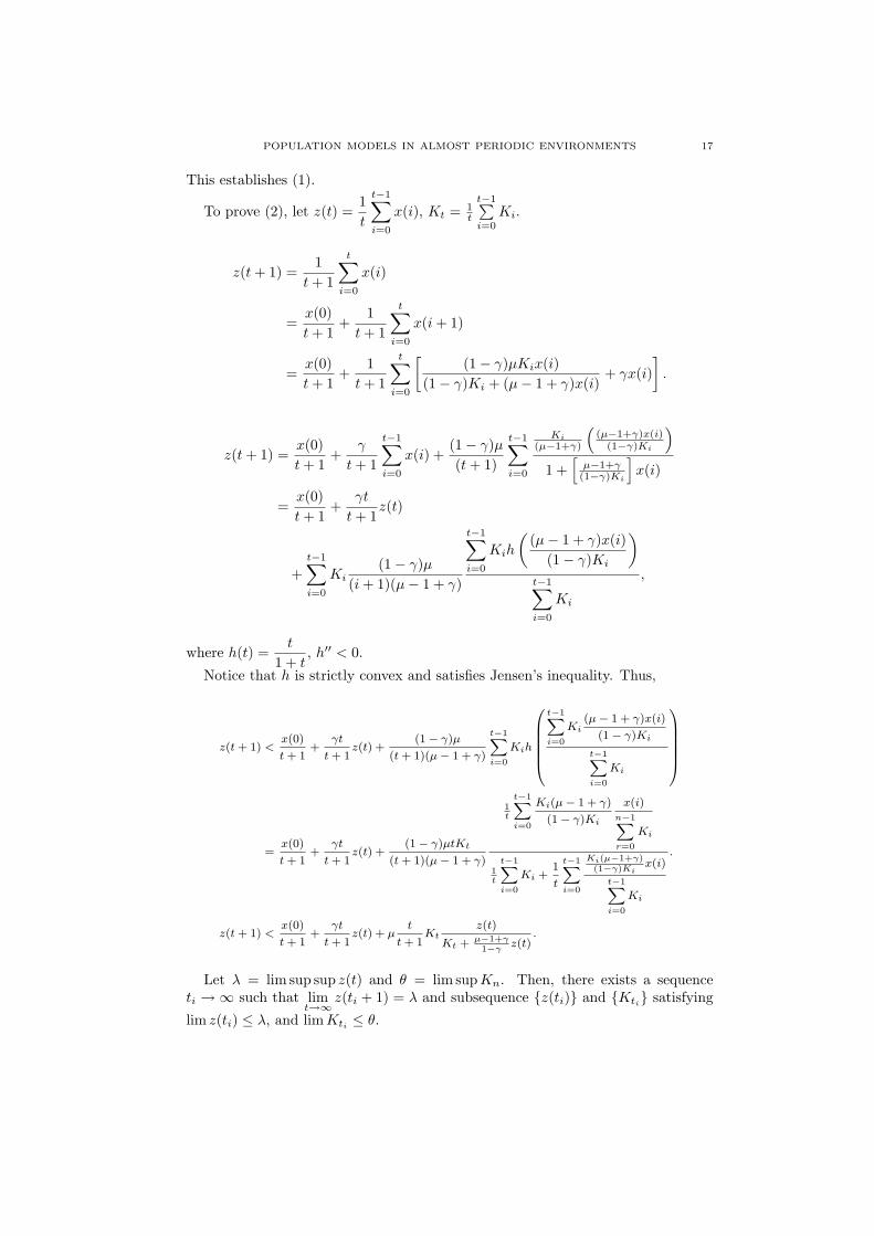
This establishes (1).
To prove (2), let z(t) =1t
t−1∑
i=0
x(i), Kt = 1t
t−1∑i=0
Ki.
z(t + 1) =1
t + 1
t∑
i=0
x(i)
=x(0)t + 1
+1
t + 1
t∑
i=0
x(i + 1)
=x(0)t + 1
+1
t + 1
t∑
i=0
[(1− γ)µKix(i)
(1− γ)Ki + (µ− 1 + γ)x(i)+ γx(i)
].
z(t + 1) =x(0)t + 1
+γ
t + 1
t−1∑
i=0
x(i) +(1− γ)µ(t + 1)
t−1∑
i=0
Ki
(µ−1+γ)
((µ−1+γ)x(i)
(1−γ)Ki
)
1 +[
µ−1+γ(1−γ)Ki
]x(i)
=x(0)t + 1
+γt
t + 1z(t)
+t−1∑
i=0
Ki(1− γ)µ
(i + 1)(µ− 1 + γ)
t−1∑
i=0
Kih
((µ− 1 + γ)x(i)
(1− γ)Ki
)
t−1∑
i=0
Ki
,
where h(t) =t
1 + t, h′′ < 0.
Notice that h is strictly convex and satisfies Jensen’s inequality. Thus,
z(t + 1) <x(0)
t + 1+
γt
t + 1z(t) +
(1− γ)µ
(t + 1)(µ− 1 + γ)
t−1X
i=0
Kih
0BBBBB@
t−1X
i=0
Ki(µ− 1 + γ)x(i)
(1− γ)Ki
t−1X
i=0
Ki
1CCCCCA
=x(0)
t + 1+
γt
t + 1z(t) +
(1− γ)µtKt
(t + 1)(µ− 1 + γ)
1t
t−1X
i=0
Ki(µ− 1 + γ)
(1− γ)Ki
x(i)n−1X
r=0
Ki
1t
t−1X
i=0
Ki +1
t
t−1X
i=0
Ki(µ−1+γ)(1−γ)Ki
x(i)
t−1X
i=0
Ki
.
z(t + 1) <x(0)
t + 1+
γt
t + 1z(t) + µ
t
t + 1Kt
z(t)
Kt + µ−1+γ1−γ
z(t).
Let λ = lim sup sup z(t) and θ = lim sup Kn. Then, there exists a sequenceti →∞ such that lim
t→∞z(ti + 1) = λ and subsequence {z(ti)} and {Kti} satisfying
lim z(ti) ≤ λ, and lim Kti ≤ θ.
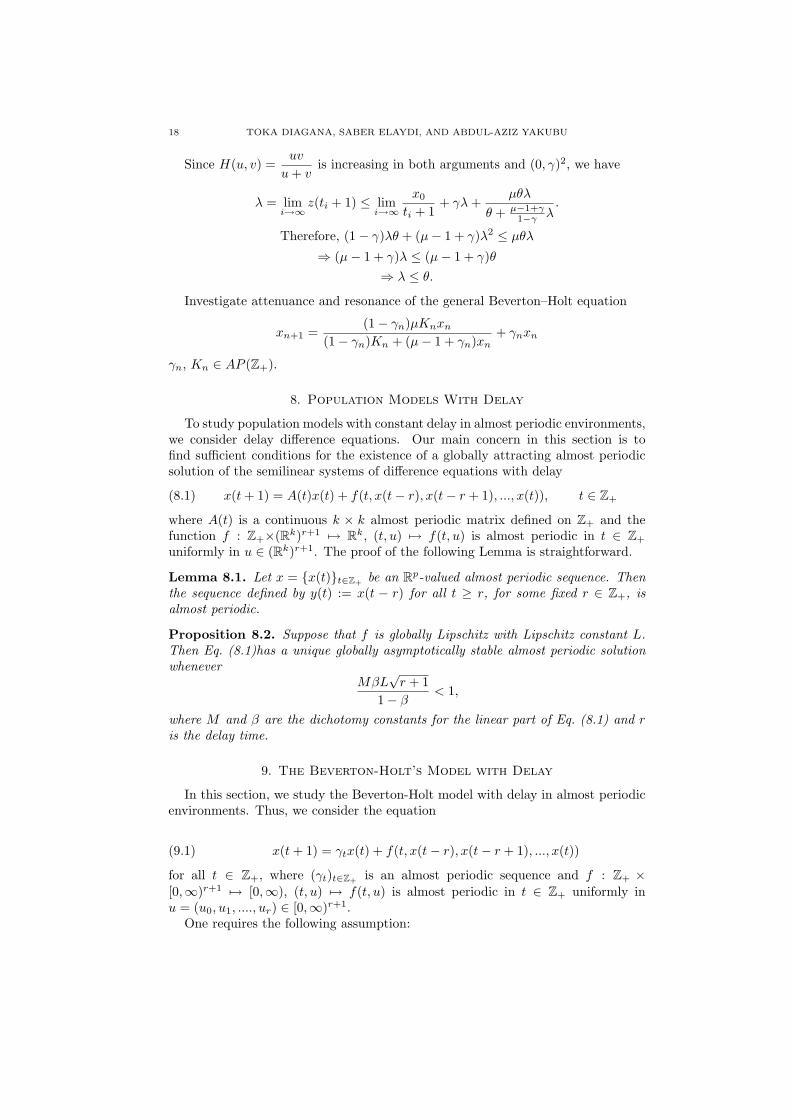
18 TOKA DIAGANA, SABER ELAYDI, AND ABDUL-AZIZ YAKUBU
Since H(u, v) =uv
u + vis increasing in both arguments and (0, γ)2, we have
λ = limi→∞
z(ti + 1) ≤ limi→∞
x0
ti + 1+ γλ +
µθλ
θ + µ−1+γ1−γ λ
.
Therefore, (1− γ)λθ + (µ− 1 + γ)λ2 ≤ µθλ
⇒ (µ− 1 + γ)λ ≤ (µ− 1 + γ)θ⇒ λ ≤ θ.
Investigate attenuance and resonance of the general Beverton–Holt equation
xn+1 =(1− γn)µKnxn
(1− γn)Kn + (µ− 1 + γn)xn+ γnxn
γn, Kn ∈ AP (Z+).
8. Population Models With Delay
To study population models with constant delay in almost periodic environments,we consider delay difference equations. Our main concern in this section is tofind sufficient conditions for the existence of a globally attracting almost periodicsolution of the semilinear systems of difference equations with delay
(8.1) x(t + 1) = A(t)x(t) + f(t, x(t− r), x(t− r + 1), ..., x(t)), t ∈ Z+
where A(t) is a continuous k × k almost periodic matrix defined on Z+ and thefunction f : Z+×(Rk)r+1 7→ Rk, (t, u) 7→ f(t, u) is almost periodic in t ∈ Z+
uniformly in u ∈ (Rk)r+1. The proof of the following Lemma is straightforward.
Lemma 8.1. Let x = {x(t)}t∈Z+ be an Rp-valued almost periodic sequence. Thenthe sequence defined by y(t) := x(t − r) for all t ≥ r, for some fixed r ∈ Z+, isalmost periodic.
Proposition 8.2. Suppose that f is globally Lipschitz with Lipschitz constant L.Then Eq. (8.1)has a unique globally asymptotically stable almost periodic solutionwhenever
MβL√
r + 11− β
< 1,
where M and β are the dichotomy constants for the linear part of Eq. (8.1) and ris the delay time.
9. The Beverton-Holt’s Model with Delay
In this section, we study the Beverton-Holt model with delay in almost periodicenvironments. Thus, we consider the equation
(9.1) x(t + 1) = γtx(t) + f(t, x(t− r), x(t− r + 1), ..., x(t))
for all t ∈ Z+, where (γt)t∈Z+ is an almost periodic sequence and f : Z+ ×[0,∞)r+1 7→ [0,∞), (t, u) 7→ f(t, u) is almost periodic in t ∈ Z+ uniformly inu = (u0, u1, ...., ur) ∈ [0,∞)r+1.
One requires the following assumption:
POPULATION MODELS IN ALMOST PERIODIC ENVIRONMENTS 19
(H) f : Z+ × [0,∞)r+1 7→ [0,∞), (t, u) 7→ f(t, u) is almost periodic in t ∈ Z+
uniformly in u ∈ [0,∞)r+1. Moreover, f is Lipschitz in u ∈ [0,∞)r+1 uniformlyin t ∈ Z+, i.e., there exists L > 0 such that
|f(t, u0, u1, ..., ur)− f(t, v0, v1, ..., vr)| ≤ L .
(r∑
k=0
|uk − vk|2)1/2
for all t ∈ Z+ and (u0, ..., ur), (v0, ..., vr) ∈ [0,∞)r+1.For instance
f(t, x) =(1− γt)µKtx
(1− γt)Kt + (µ− 1 + γt)xfor t ∈ Z+ and x ∈ [0,∞) satisfies assumption (H) whenever both (γt)t∈Z+ and(Kt)t∈Z+ are almost periodic. In that case, L = µ.
The constants of dichotomy related to Eq. (9.1) are respectively M = 1 andβ = supt∈Z+
γt ∈ (0, 1).
Corollary 9.1. Under assumption (H), Eq. (9.1) has a unique globally asymptot-ically stable almost periodic solution whenever
β <1
1 + L√
r + 1.
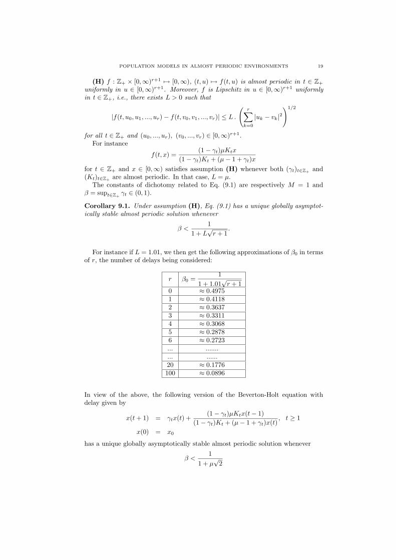
For instance if L = 1.01, we then get the following approximations of β0 in termsof r, the number of delays being considered:
r β0 =1
1 + 1.01√
r + 10 ≈ 0.49751 ≈ 0.41182 ≈ 0.36373 ≈ 0.33114 ≈ 0.30685 ≈ 0.28786 ≈ 0.2723... .......... ......20 ≈ 0.1776100 ≈ 0.0896
In view of the above, the following version of the Beverton-Holt equation withdelay given by
x(t + 1) = γtx(t) +(1− γt)µKtx(t− 1)
(1− γt)Kt + (µ− 1 + γt)x(t), t ≥ 1
x(0) = x0
has a unique globally asymptotically stable almost periodic solution whenever
β <1
1 + µ√
2
20 TOKA DIAGANA, SABER ELAYDI, AND ABDUL-AZIZ YAKUBU
with µ > 1. However, if we consider the original version of Beverton-Holt equationwith delay in the form
x(t + 1) = γtx(t) +(1− γt)µKtx(t− 1)
(1− γt)Kt + (µ− 1 + γt)x(t− 1), t ≥ 1
x(0) = x0
we obtain a better result if we convert the equation into a two-dimensional systemwith no delay and apply Theorem 4.6 directly. It follows that this equation has aunique globally asymptotically stable almost periodic solution whenever
β <1
1 + µ
with µ > 1.
10. Conclusion
Almost periodic deterministic models are more likely to capture the “noise”associated with real-population data. Using these models, we study the effectsof almost periodic forcing of the carrying capacity, the demographic characteristicand survival rates of species on the long-term behavior of discretely reproducingpopulations. Others have studied the effects of periodic forcing of the carryingcapacity, the demographic characteristic and survival rates of species on populationdynamics [8, 9, 10], [12, 13, 14, 15, 16], [20, 21, 22, 23, 24], [28, 29, 30, 31], and[34, 35, 36, 37]. Typically, such periodically forced models support attracting cyclesthat are either enhance via resonance or diminished via attenuance.
In almost periodic environments, simple population models support a globallyattracting almost periodic solution. Developing a signature function for determiningwhether the almost periodic solution is attenuance or resonance is an interestingquestion that we plan to explore elsewhere.
References
1. S. B. Angenent, The zero set of a parabolic differential equation, J. Reine Agnew. Math. 390(1988), 79–96.
2. W. Arendt, C. Batty, M. Hieber, and F. Neubrander, Vector-valued Laplace Transforms andCauchy Problems, Monographs in Mathematics, Birkhauser, 2001.
3. M. Begon, J. L. Harper and C. R. Townsend, Ecology: individuals, populations and communi-ties, Blackwell Science Ltd (1996).
4. J. Blot and D. Pennequin, Existence and Structure Results on Almost Periodic Solutions ofDifference Equations, J. Differ. Equations Appl.7 (2001), no. 3, 383–402
5. R. C. Casten and C. J. Holland, Instability results for reaction-diffusion equations with Neu-mann boundary conditions, J. Differential Equations. 27 (1978), no. 2, 266–273.
6. C. Corduneanu, Almost periodic functions, 2nd Edition, Chelsea-New York, 1989.7. R. F. Costantino, J. M. Cushing, B. Dennis and R. A. Desharnais, Resonant popopulation
cycles in temporarily fluctuating habitats, Bull. Math. Biol. 60(1998), 247-273.8. J. M. Cushing, Periodic time-dependent predator-prey systems, SIAM J. Appl. Math. 32
(1977), 82-95.9. J. M. Cushing, The LPA model, Fields Institute Communications 43 (2004), 29-55.10. J. M. Cushing and S. M. Henson, Global dynamics of some periodically forced, monotone
difference equations, J. Diff. Equations Appl. 7 (2001), 859-872.11. S. N. Elaydi, Discrete Chaos. Chapman & Hall/CRC, Boca Raton, FL (2000).12. S. N. Elaydi, Periodicity and stability of linear Volterra difference equations, J. Math. Anal.
Appl. 181(1994), 483-492.
POPULATION MODELS IN ALMOST PERIODIC ENVIRONMENTS 21
13. S. N. Elaydi and R. J. Sacker, Global Stability of Periodic Orbits of Nonautonomous DifferenceEquations and Population Biology, J. Differential Equations 208(2005), 258-273.
14. S. N. Elaydi and R. J. Sacker, Global Stability of Periodic Orbits of Nonautonomous DifferenceEquations in Population Biology and the Cushing-Henson conjectures, Proceedings of the EighthInternational Conference on Difference Equations and Applications, Chapman & Hall / CRC,Boca Raton, FL, 2005, 113–126.
15. S. N. Elaydi and R. J. Sacker, Global Stability of Periodic Orbits of Nonautonomous DifferenceEquations In Population Biology and Cushing-Henson Conjectures, J. Diff. Equations Appl. 11(2005), no. 4-5, 337-346.
16. S. N. Elaydi and R. J. Sacker, Nonautonomous Beverton-Holt Equations and the Cushing-Henson Conjectures, J. Diff. Equations Appl. 11 (2005), 337-347.
17. S. N. Elaydi and A.-A. Yakubu, Global Stability of Cycles: Lotka-Volterra Competition ModelWith Stocking, J. Diff. Equations Appl. 8 (2002), no. 6, 537-549.
18. Ky Fan, Les fonctions asymptotiquement presque-periodiques d’une variable entiere et leurapplication a l’etude de l’iteration des transformations continues, Math. Z. 48 (1943), 685-711.
19. A. M. Fink, Almost Periodic Differential Equations, Lecture Notes in Mathematics 377,Springer-Verlag, New York-Berlin, 1974.
20. J. E. Franke and J. F. Selgrade, Attractor for Periodic Dynamical Systems, J. Math. Anal.Appl. 286 (2003), 64-79.
21. J. E. Franke and A.-A. Yakubu, Discrete-time metapopulation dynamics and unidirectionaldispersal, J. Diff. Equations Appl. 9 (2003), no. 7, 633-653.
22. J. E. Franke and A.-A. Yakubu, Multiple Attractors Via Cusp Bifurcation In PeriodicallyVarying Environments, J. Diff. Equations Appl. 11 (2002), no. 4-5, 365-377.
23. J. E. Franke and A.-A. Yakubu, Population models with periodic recruitment functions andsurvival rates, J. Diff. Equations Appl. 11 (2005), no. 14, 1169-1184.
24. J. E. Franke and A.-A. Yakubu, Signature functions for predicting resonant and attenuantpopulation cycles. Bull. Math. Biol. (In press).
25. A. Halanay and V. Rasvan, Stability and stable oscillations in discrete time systems, Advancesin Discrete Mathematics and Applications, Vol. 2, Gordon and Breach Science Publication, 2000.
26. M. P. Hassell, The dynamics of competition and predation, Studies in Biol. 72(1976), TheCamelot Press Ltd.
27. D. Henry, Geometric theory of semilinear parabolic equations, Lecture Notes in Mathematics840, Springer-Verlag, New York-Berlin, 1981.
28. S. M. Henson, Multiple attractors and resonance in periodically forced population models,Physics D. 140(2000), 33-49.
29. S. M. Henson, R. F. Costantino, J. M. Cushing, B. Dennis and R. A. Desharnais, Multipleattractors, saddles, and population dynamics in periodic habitats, Bull. Math. Biol. 61 (1999),1121-1149.
30. S. M. Henson and J. M. Cushing, The effect of periodic habitat fluctuations on a nonlinearinsect population model, J. Math. Biol. 36 (1997), 201-226.
31. S. M. Henson et al., Predicting dynamics of aggregate loafing behavior in Glaucose-WingedGulls (Larus-Glaucoscens) at a Washington Colony, The AUK 121 (2004).
32. M. Hirsch, Attractors for discrete-time monotone systems in strongly ordered spaces, Geom-etry and topology, Lecture Notes in Mathematics, 1167, Springer, Berlin (1985).
33. R. Jajte, Almost periodic sequences. Colloq. Math. 12 1964/1965, 235–267.34. D. Jillson, Insect populations respond to fluctuating environments, Nature 288(1980), 699-
700.35. V. L. Kocic, A note on nonautonomous Beverton-Holt model, J. Diff. Equations Appl., to
appear.36. R. Kon, A note on attenuant cycles of population models with periodic carrying capacity, J.
Diff. Equations Appl., to appear.37. R. Kon, Attenuant cycles of population models with periodic carrying capacity, J. Diff. Equa-
tions Appl., to appear.38. J. Li, Periodic solutions of population models in a periodically fluctuating environment, Math.
Biosc. 110 (1992), 17-25.39. E. Liz and J. B. Ferreiro, A note on the global stability of generalized difference equations,
Appl. Math. Lett 15 (2002), 655-659.
22 TOKA DIAGANA, SABER ELAYDI, AND ABDUL-AZIZ YAKUBU
40. R. M. May, Simple mathematical models with very complicated dynamics, Nature 261(1977),459-469.
41. R. M. May, Stability and complexity in model ecosystems, Princeton University Press, 1974.42. R. K. Miller, Almost periodic differential equations as dynamical systems with applications
to the existence of a. p. solutions, Journal of Differential Equations,1 (1965).43. A. Muchnik, A. Semonov, and M. Ushakov, Almost Periodic Sequences, Theoretical Comp.
Sci. 304 (2003), 1–33.44. D. Pennequin, Existence of Almost Periodic Solutions of Discrete Time Equations, Discrete
and Continuous Dynamical Systems. 7 (2001), no. 1, 51-80.45. W. E. Ricker, Stock and recruitment, Journal of Fisheries Research Board of Canada II(5)
(1954), 559-623.46. R. J. Sacker and G. Sell, Lifting properties in skew-product flows with applications to Dif-
ferential Equations, Mem. Amer. Math. Soc. 11 (1977), no. 190, iv+67 pp.
Department of Mathematics, Howard University, 2441 6th Street N.W., WashingtonD.C. 20059
E-mail address: [email protected]
Department of Mathematics, Trinity University, San Antonio, TX 78212E-mail address: [email protected]
Department of Mathematics, Howard University, 2441 6th Street N.W., WashingtonD.C. 20059
E-mail address: [email protected]


![A Various Types of Almost Periodic Functions on Banach Spaces: … · 2011-02-23 · Bochner introduced the concept of almost automorphic functions in his papers [22], [23] and](https://img.pdfslide.us/doc/110x75/5fb2c51e1f4b03320f318042/a-various-types-of-almost-periodic-functions-on-banach-spaces-2011-02-23-bochner.jpg)
![arxiv.org · arXiv:1104.4851v1 [math.FA] 26 Apr 2011 REPRESENTATIONS OF ALMOST PERIODIC PSEUDODIFFERENTIAL OPERATORS AND APPLICATIONS IN SPECTRAL THEORY PATRIK WAHLBERG Abstract](https://img.pdfslide.us/doc/110x75/5f916e7cec826d5adf5c737e/arxivorg-arxiv11044851v1-mathfa-26-apr-2011-representations-of-almost-periodic.jpg)