Embed Size (px)
Citation preview
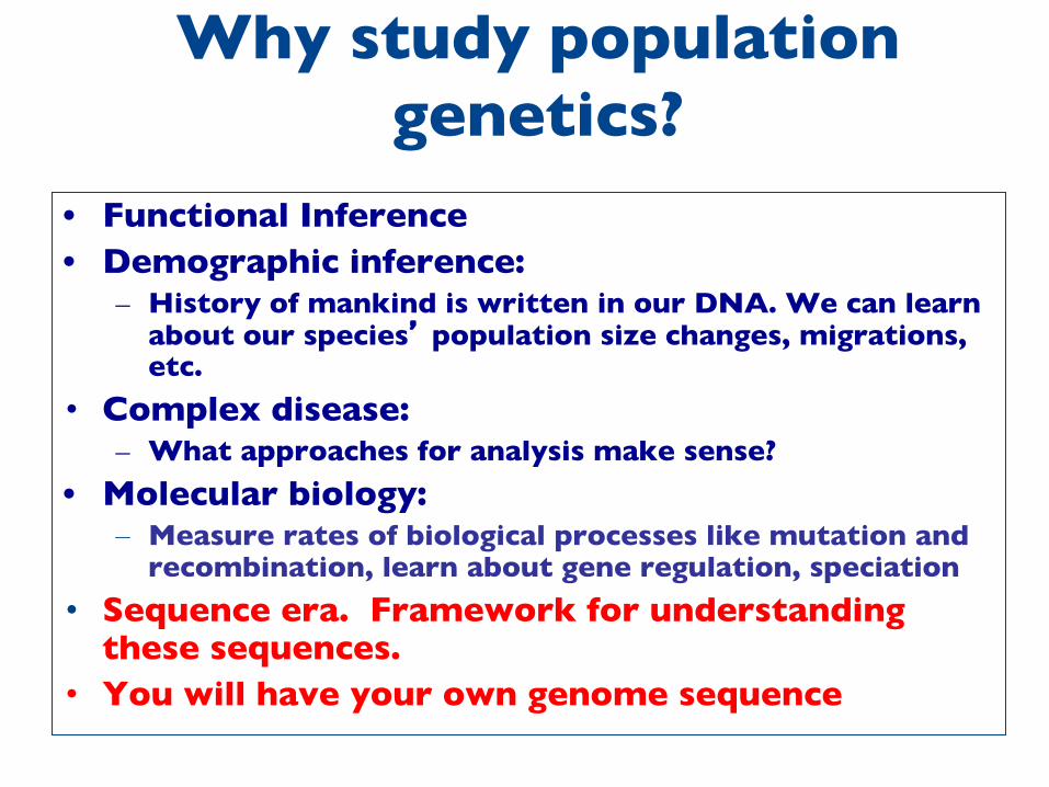
Why study population genetics?
• Functional Inference• Demographic inference:
– History of mankind is written in our DNA. We can learn about our species’ population size changes, migrations, etc.
• Complex disease:– What approaches for analysis make sense?
• Molecular biology:– Measure rates of biological processes like mutation and
recombination, learn about gene regulation, speciation • Sequence era. Framework for understanding
these sequences.• You will have your own genome sequence
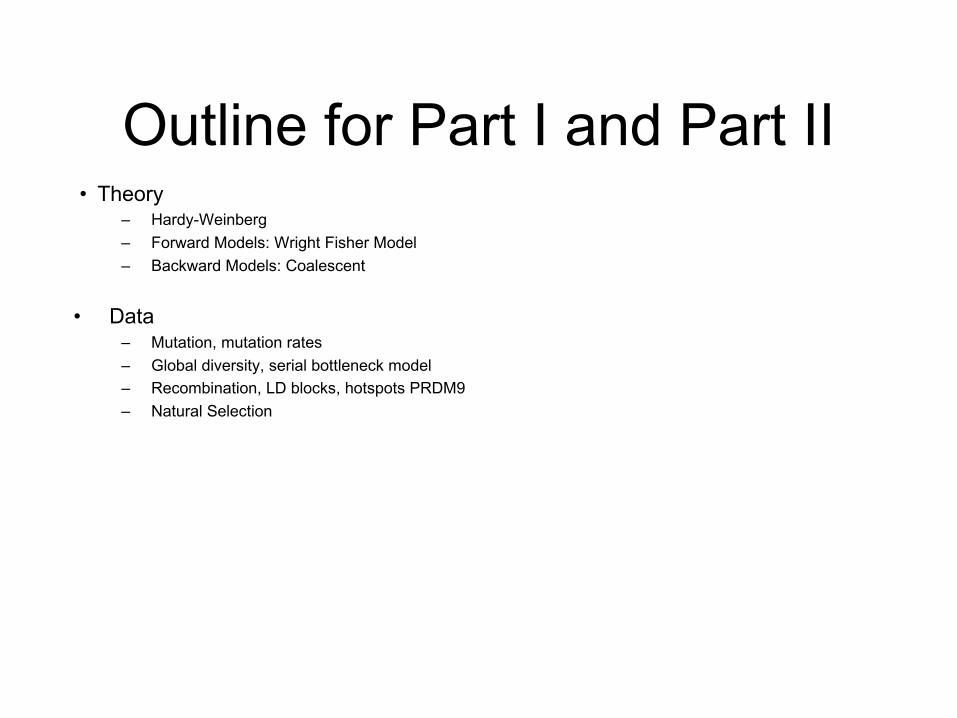
Outline for Part I and Part II• Theory
– Hardy-Weinberg– Forward Models: Wright Fisher Model– Backward Models: Coalescent
• Data– Mutation, mutation rates – Global diversity, serial bottleneck model – Recombination, LD blocks, hotspots PRDM9– Natural Selection
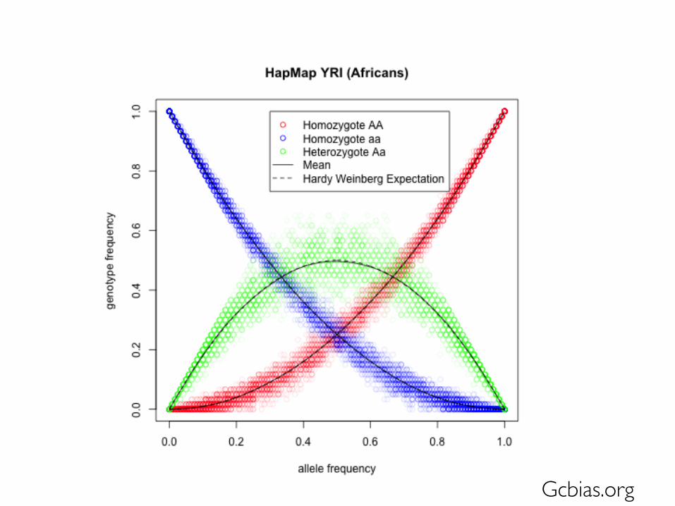
Hardy-Weinberg
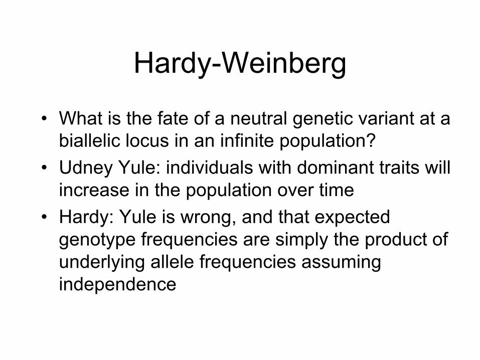
• What is the fate of a neutral genetic variant at a biallelic locus in an infinite population?
• Udney Yule: individuals with dominant traits will increase in the population over time
• Hardy: Yule is wrong, and that expected genotype frequencies are simply the product of underlying allele frequencies assuming independence
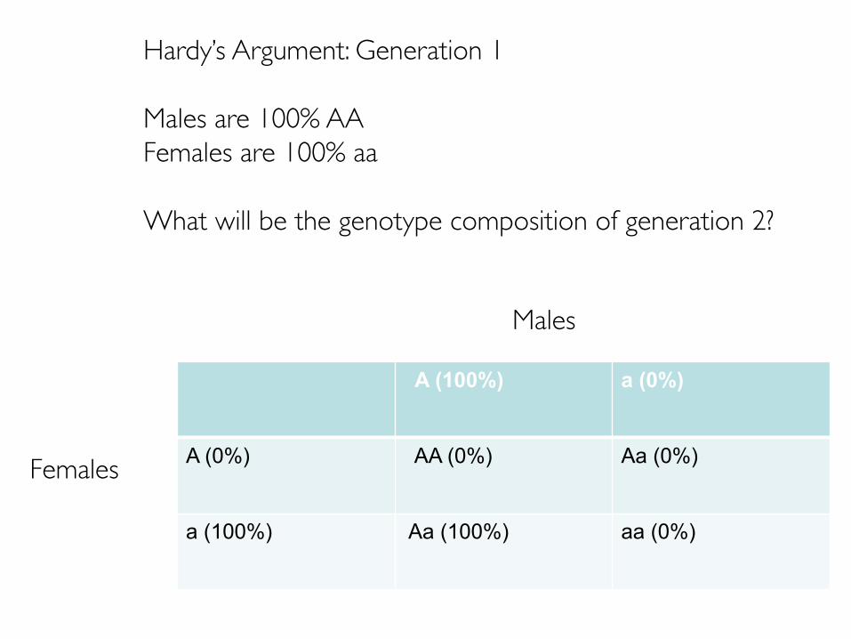
A (100%) a (0%)
A (0%) AA (0%) Aa (0%)
a (100%) Aa (100%) aa (0%)
Hardy’s Argument: Generation 1
Males are 100% AAFemales are 100% aa
What will be the genotype composition of generation 2?
Males
Females
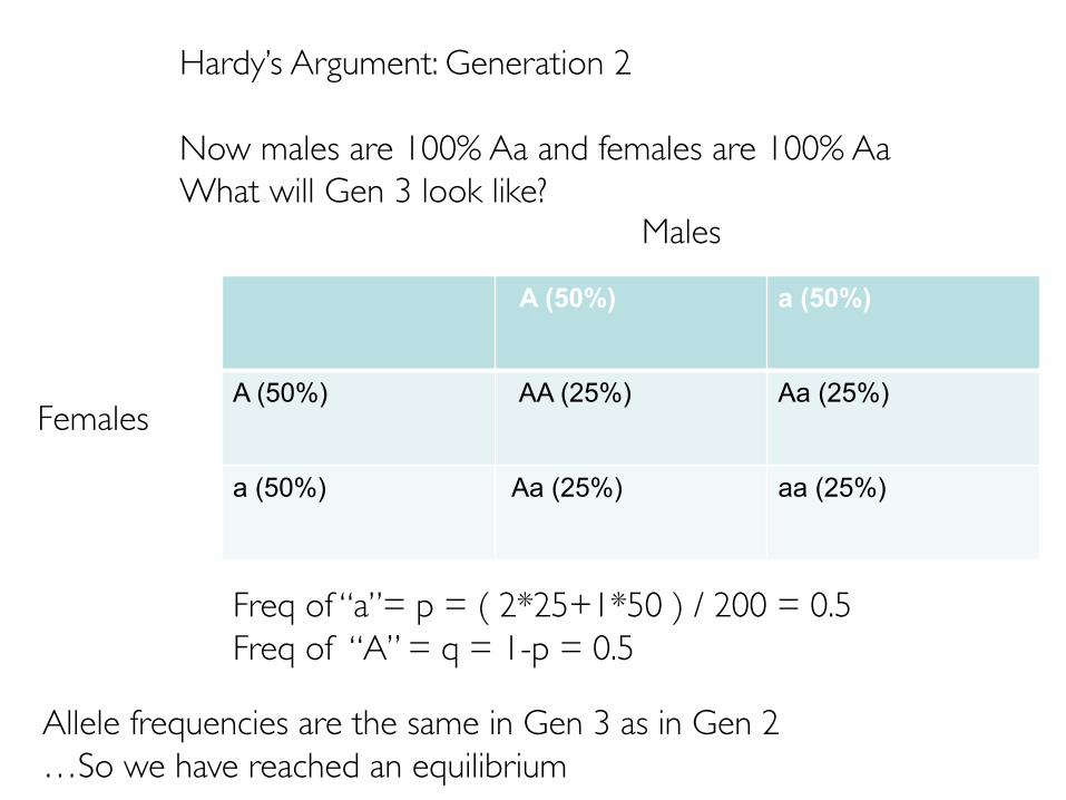
A (50%) a (50%)
A (50%) AA (25%) Aa (25%)
a (50%) Aa (25%) aa (25%)
Allele frequencies are the same in Gen 3 as in Gen 2…So we have reached an equilibrium
Hardy’s Argument: Generation 2
Now males are 100% Aa and females are 100% AaWhat will Gen 3 look like?
Males
Females
Freq of “a”= p = ( 2*25+1*50 ) / 200 = 0.5Freq of “A” = q = 1-p = 0.5
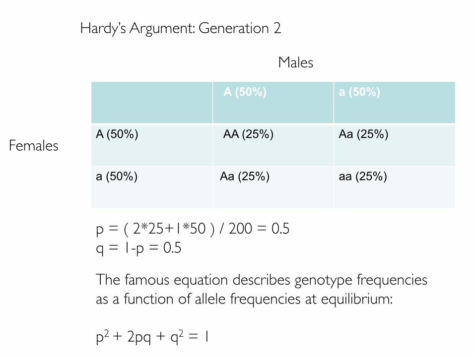
A (50%) a (50%)
A (50%) AA (25%) Aa (25%)
a (50%) Aa (25%) aa (25%)
The famous equation describes genotype frequencies as a function of allele frequencies at equilibrium:
p2 + 2pq + q2 = 1
Hardy’s Argument: Generation 2
Males
Females
p = ( 2*25+1*50 ) / 200 = 0.5q = 1-p = 0.5
Gcbias.org
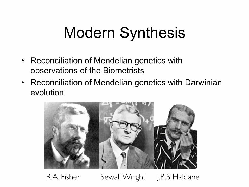
Modern Synthesis• Reconciliation of Mendelian genetics with
observations of the Biometrists• Reconciliation of Mendelian genetics with Darwinian
evolution
R.A. Fisher Sewall Wright J.B.S Haldane

Wright-Fisher ModelAssumptions:• Two allele system• N diploid individuals in each generation• 2N gametes• Random mating, no selection• Discrete generations
Aa
Generationt
t + 1
Aa
aA
a
A
AA
aaGamete pool
Let’s play a round of this game
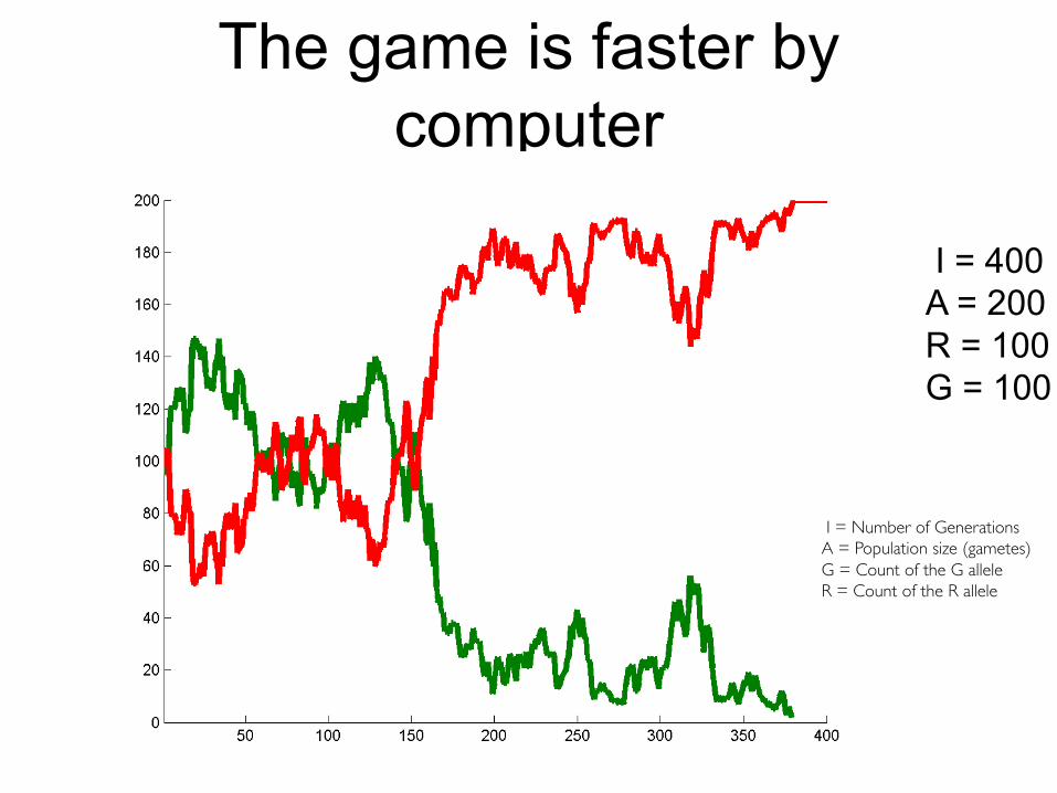
The game is faster by computer
I = 400A = 200R = 100G = 100
I = Number of GenerationsA = Population size (gametes)G = Count of the G alleleR = Count of the R allele
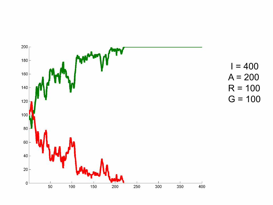
I = 400A = 200R = 100G = 100

I = 400A = 200R = 100G = 100

Let’s investigate this phenomenon
• Change Population Size
• Change allele frequencies
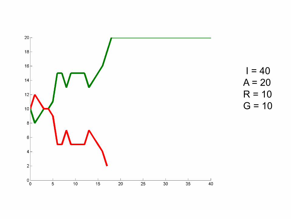
I = 40A = 20R = 10G = 10
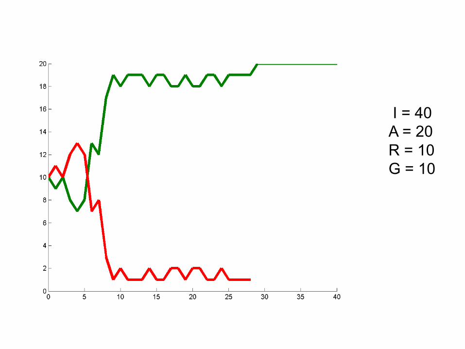
I = 40A = 20R = 10G = 10
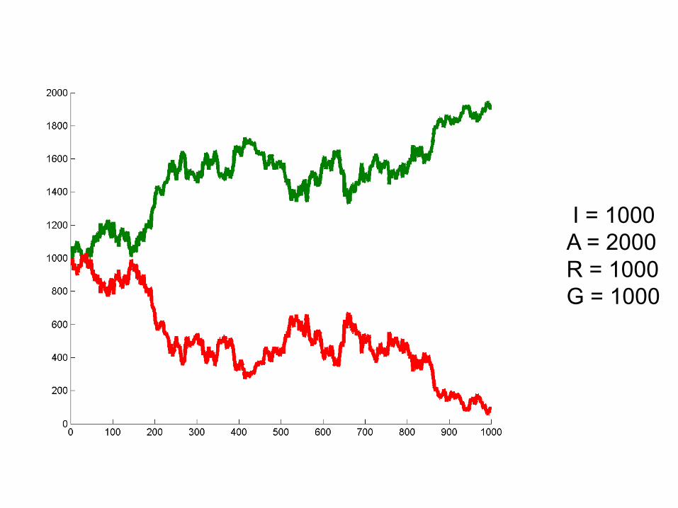
I = 1000A = 2000R = 1000G = 1000
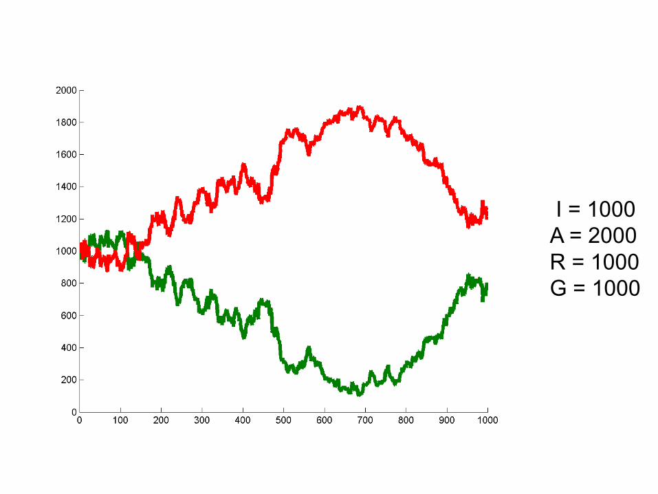
I = 1000A = 2000R = 1000G = 1000
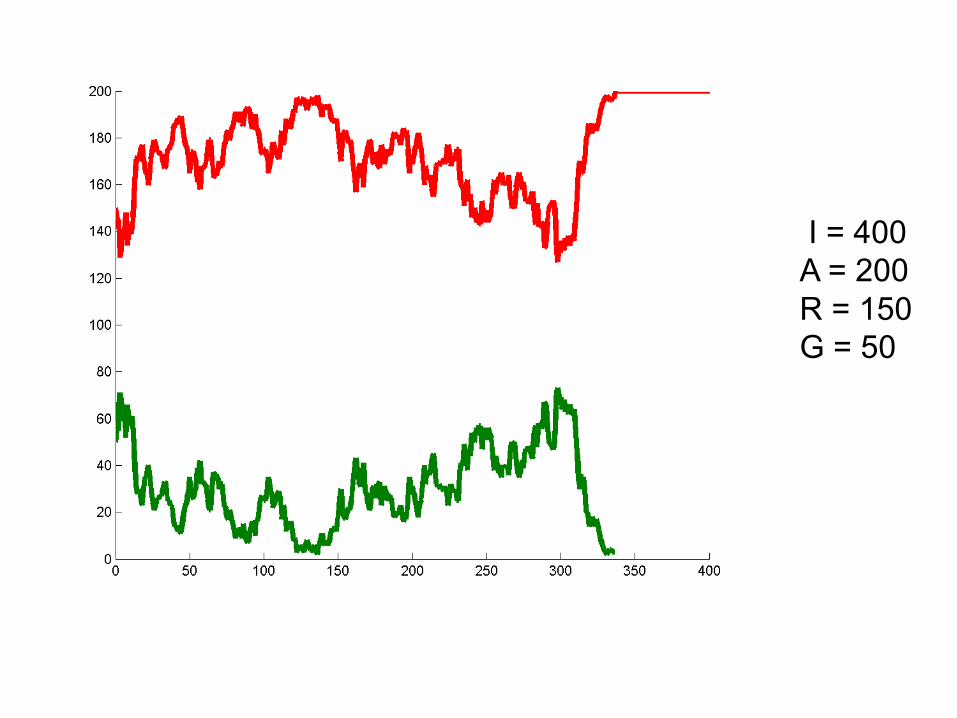
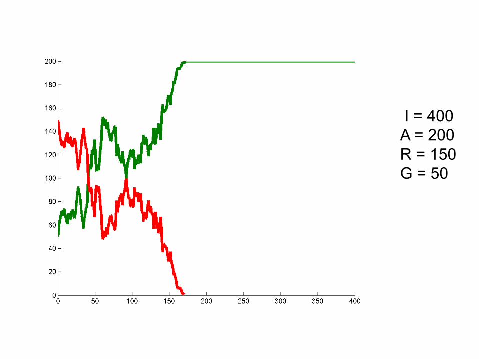
I = 400A = 200R = 150G = 50

I = 400A = 200R = 150G = 50
I = 400A = 200R = 150G = 50
Can we deduce general rules?
• Larger population size = alleles stick around longer. Less susceptibility to “random walk”
• Probability of winning seems related to initial frequencies. At 50/50 50% chance of either allele winning. Hypothesize: probability of winning is proportional to initial frequency.
• Hypothesis: One allele must always win.
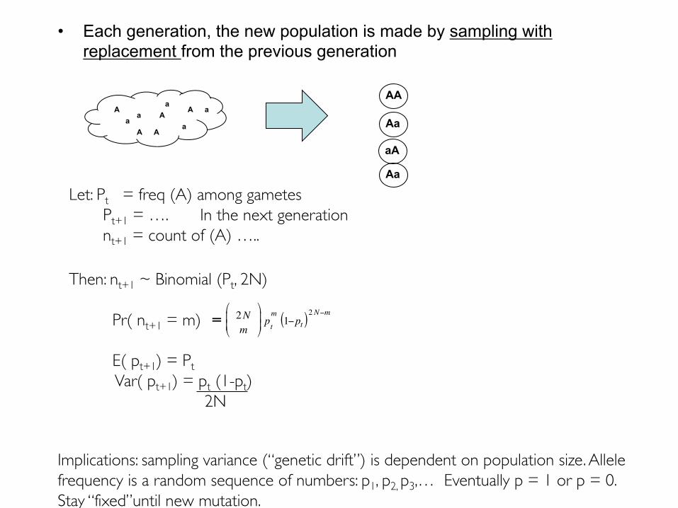
• Each generation, the new population is made by sampling with replacement from the previous generation
Aa
aA
a
A
AA
aa
aA
Aa
AA
Aa
Let: Pt = freq (A) among gametesPt+1 = …. In the next generationnt+1 = count of (A) …..
Then: nt+1 ~ Binomial (Pt, 2N)
Pr( nt+1 = m)
E( pt+1) = PtVar( pt+1) = pt (1-pt)
2N
= 2Nm
!
"##
$
%&& pt
m1−pt( )2N−m
Implications: sampling variance (“genetic drift”) is dependent on population size. Allele frequency is a random sequence of numbers: p1, p2, p3,… Eventually p = 1 or p = 0. Stay “fixed”until new mutation.

An important concept: Drift
• Drift – stochastic fluctuations in allele frequency due to random sampling in a finite population.

Drift versus Darwin
• How can we add selection to our game?
• We need to account for dominant and recessive alleles!
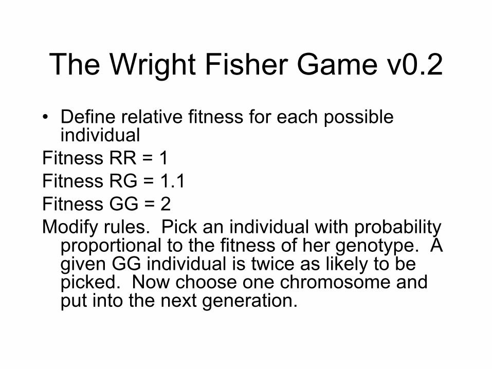
The Wright Fisher Game v0.2• Define relative fitness for each possible
individualFitness RR = 1Fitness RG = 1.1Fitness GG = 2Modify rules. Pick an individual with probability
proportional to the fitness of her genotype. A given GG individual is twice as likely to be picked. Now choose one chromosome and put into the next generation.
What relative fitness should we select?
• Conserved elements <0.01% increase in fitness
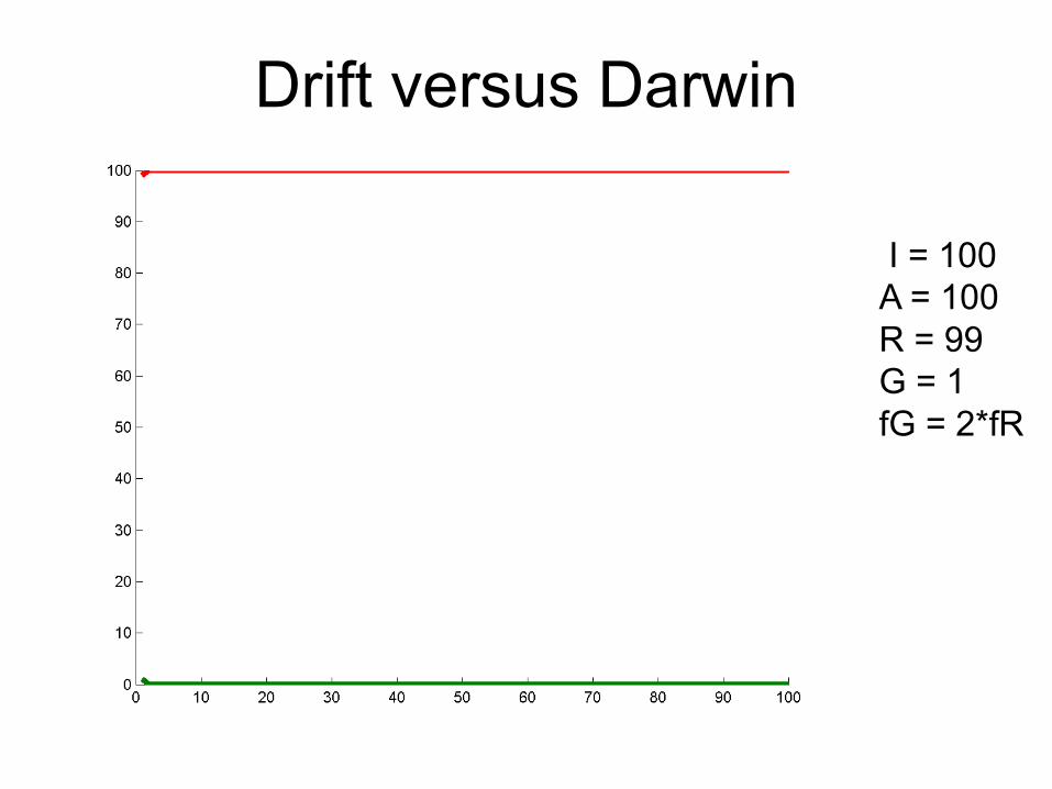
Drift versus Darwin
I = 100A = 100R = 99G = 1fG = 2*fR

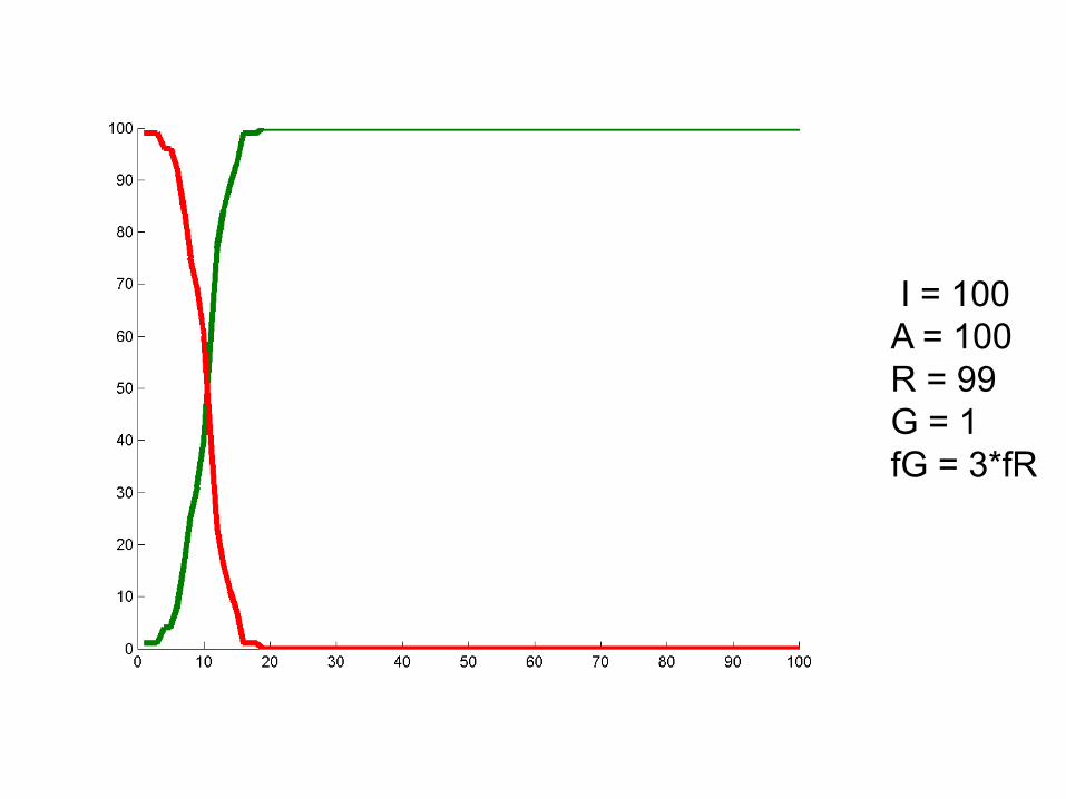
I = 100A = 100R = 99G = 1fG = 3*fR
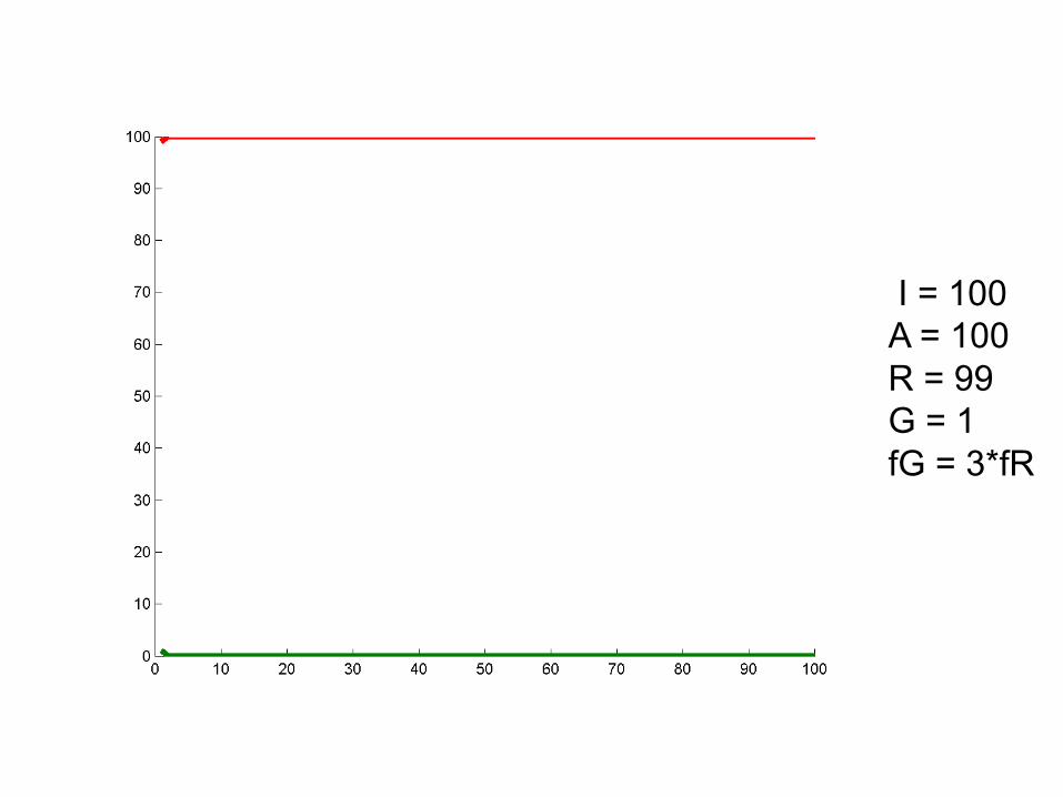
I = 100A = 100R = 99G = 1fG = 3*fR
I = 100A = 100R = 99G = 1fG = 3*fR
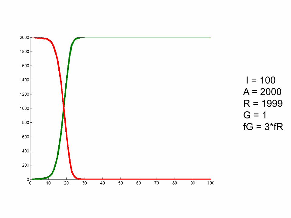
I = 100A = 2000R = 1999G = 1fG = 3*fR
Some startling results!
• Survival of the fittest luckiest.
• Sometimes drift can overcome selection. Depends on allele frequency, population size.
• Most new advantageous mutations are not fixed!
Mutation
• Infinite alleles model– Assumptions
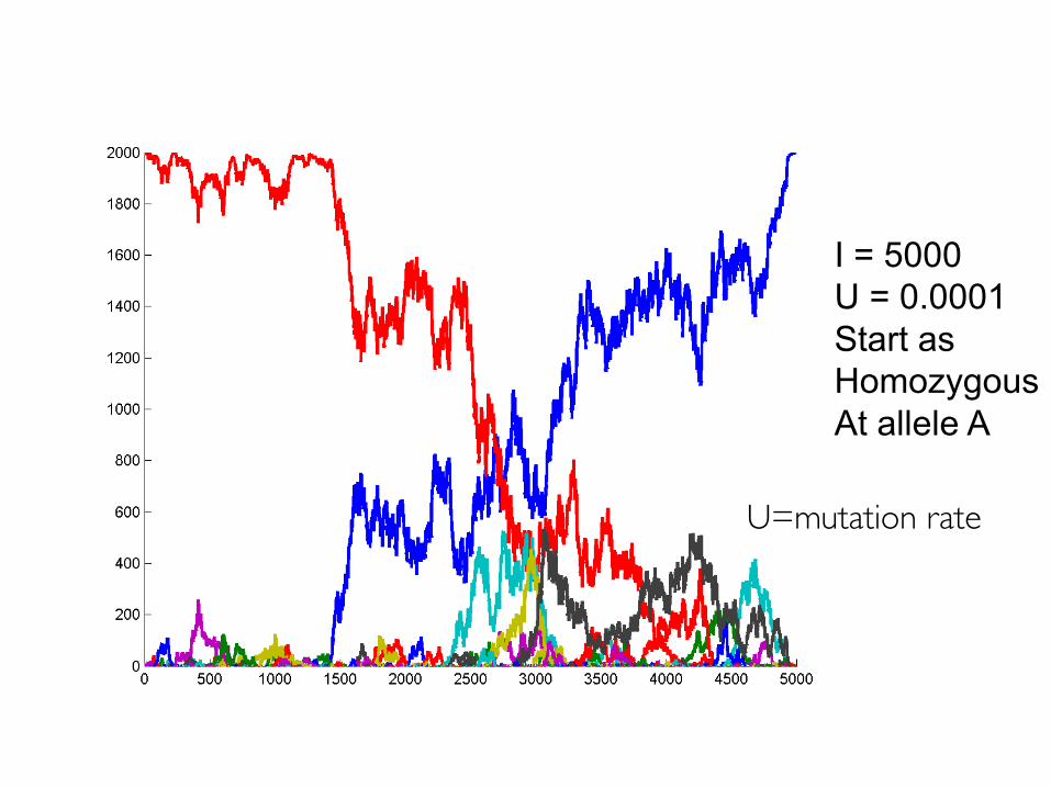
I = 5000U = 0.0001Start as HomozygousAt allele A
U=mutation rate
Summary thus far• Chance can play a large role in determining which
polymorphisms are fixed in a population.
• The fittest don’t always survive.
• These findings are/were not obvious.
• They become (more) obvious with quantitative investigation.
• And we’ve only scratched the surface.
Further explorations of this model
• To date our approach has been based on observations of simulations. But the model is simple – analytic approach may prove fruitful.
• Our hypotheses:– Can we prove them?
– Can we quantify them?
• Lets explore this hypothesis: One allele must always win.
The Decay of Heterozygosity
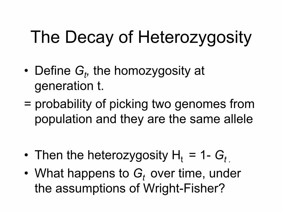
• Define Gt, the homozygosity at generation t.
= probability of picking two genomes from population and they are the same allele
• Then the heterozygosity Ht = 1- Gt .
• What happens to Gt over time, under the assumptions of Wright-Fisher?

What is G0
RB
RB BB
BB
Generation 0
1. Pick R then R
= number of R’s / 2N* number Rs-1 / (2N-1)
2. Pick B then B
= number of B’s / 2N)* (number B’s-1) / (2N-1)
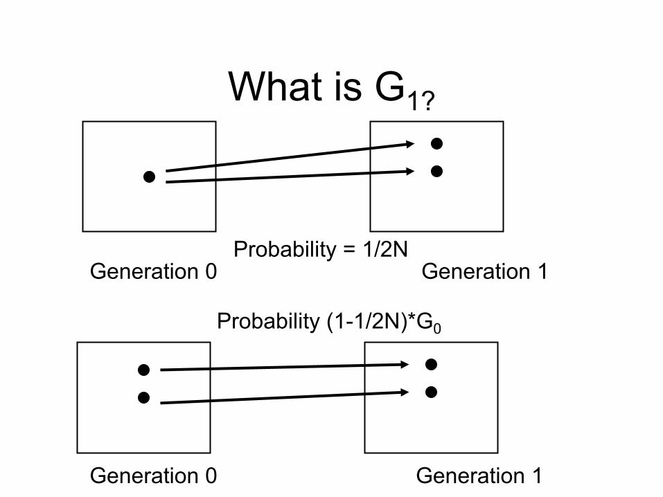
What is G1?
Probability = 1/2N
Probability (1-1/2N)*G0
Generation 0 Generation 1
Generation 0 Generation 1

Proof of decay of heterozygosity
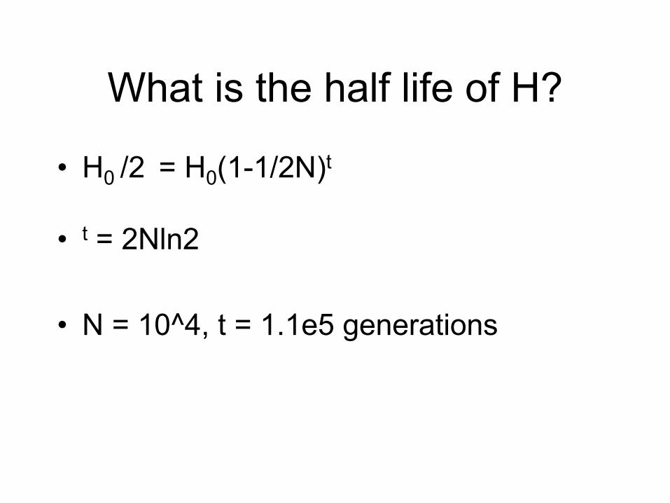
What is the half life of H?
• H0 /2 = H0(1-1/2N)t
• t = 2Nln2
• N = 10^4, t = 1.1e5 generations
What does this mean?
• In a large population, eventually, every allele will have descended from a single allele in the founding population! All but 1 allele will have “died off”.
• Drift-Mutation-Selection balance.

-Genealogical Analysis of all 131K Icelanders born after 1972
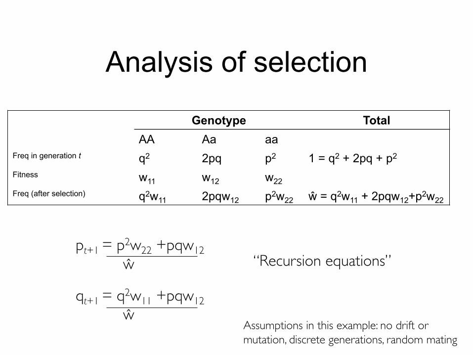
Analysis of selection
Genotype TotalAA Aa aa
Freq in generation t q2 2pq p2 1 = q2 + 2pq + p2
Fitness w11 w12 w22Freq (after selection) q2w11 2pqw12 p2w22 ŵ = q2w11 + 2pqw12+p2w22
pt+1 = p2w22 +pqw12ŵ
qt+1 = q2w11 +pqw12ŵ
“Recursion equations”
Assumptions in this example: no drift or mutation, discrete generations, random mating
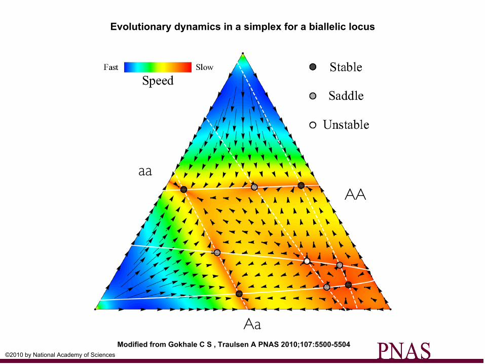
Evolutionary dynamics in a simplex for a biallelic locus
Modified from Gokhale C S , Traulsen A PNAS 2010;107:5500-5504©2010 by National Academy of Sciences
AA
Aa
aa
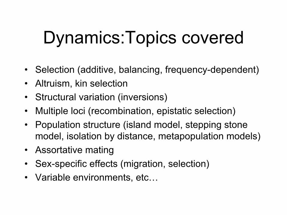
Dynamics:Topics covered• Selection (additive, balancing, frequency-dependent)• Altruism, kin selection• Structural variation (inversions)• Multiple loci (recombination, epistatic selection)• Population structure (island model, stepping stone
model, isolation by distance, metapopulation models)• Assortative mating• Sex-specific effects (migration, selection)• Variable environments, etc…

Sampling with Replacement• Some alleles pass
on no copies to the next generation, while some pass on more than one.
Present
Past
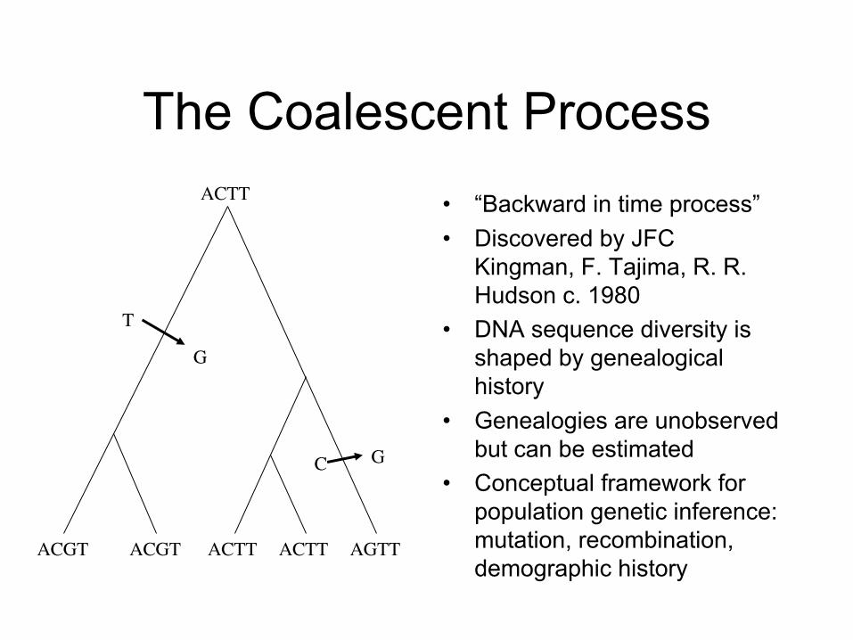
The Coalescent Process• “Backward in time process”• Discovered by JFC
Kingman, F. Tajima, R. R. Hudson c. 1980
• DNA sequence diversity is shaped by genealogical history
• Genealogies are unobserved but can be estimated
• Conceptual framework for population genetic inference: mutation, recombination, demographic history
ACTT
ACGT ACGT ACTT ACTT AGTT
T
G
C G