Embed Size (px)
Citation preview

Population Genetics
I. Basic Principles

Population Genetics
I. Basic Principles
A. Definitions:- Population: a group of interbreeding organisms that share a
common gene pool; spatiotemporally and genetically defined - Gene Pool: sum total of alleles held by individuals in a population - Gene/Allele Frequency: % of genes at a locus of a particular allele - Gene Array: % of all alleles at a locus: must sum to 1. - Genotypic Frequency: % of individuals with a particular genotype - Genotypic Array: % of all genotypes for loci considered = 1.
Population Genetics
I. Basic Principles
A. Definitions: B. Basic computations:
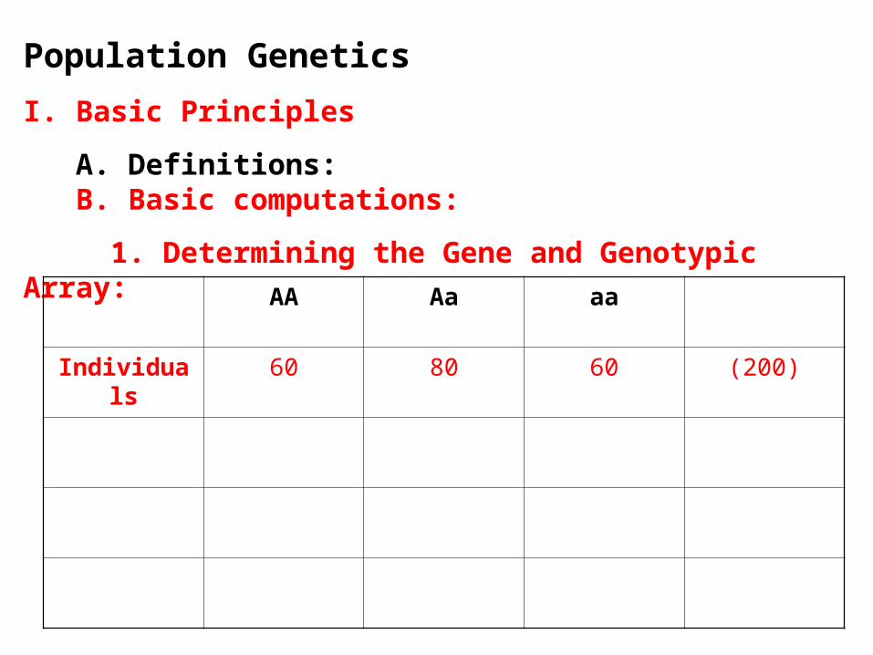
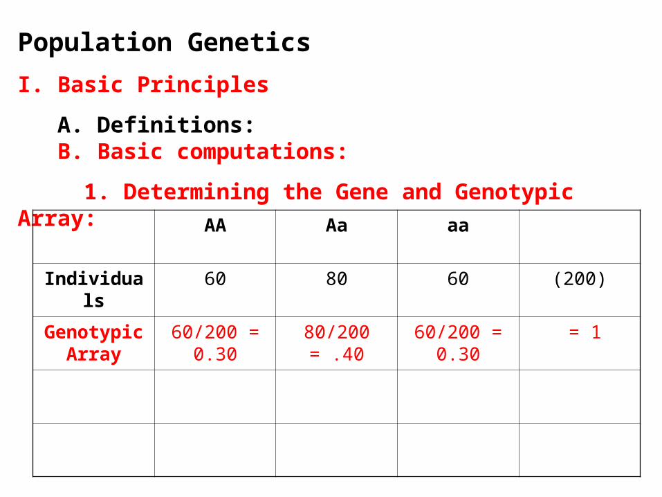
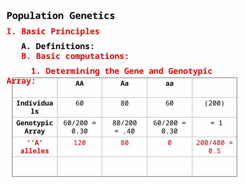
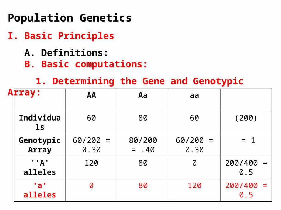
1. Determining the Gene and Genotypic Array:
AA Aa aa
Individuals 60 80 60 (200)
Population Genetics
I. Basic Principles
A. Definitions: B. Basic computations:
1. Determining the Gene and Genotypic Array:
AA Aa aa
Individuals 60 80 60 (200)
Genotypic Array
60/200 = 0.30
80/200 = .40 60/200 = 0.30
= 1
Population Genetics
I. Basic Principles
A. Definitions: B. Basic computations:
1. Determining the Gene and Genotypic Array:
AA Aa aa
Individuals 60 80 60 (200)
Genotypic Array
60/200 = 0.30
80/200 = .40 60/200 = 0.30
= 1
''A' alleles 120 80 0 200/400 = 0.5
Population Genetics
I. Basic Principles
A. Definitions: B. Basic computations:
1. Determining the Gene and Genotypic Array:
AA Aa aa
Individuals 60 80 60 (200)
Genotypic Array
60/200 = 0.30
80/200 = .40 60/200 = 0.30
= 1
''A' alleles 120 80 0 200/400 = 0.5
'a' alleles 0 80 120 200/400 = 0.5
Population Genetics
I. Basic Principles
A. Definitions: B. Basic computations:
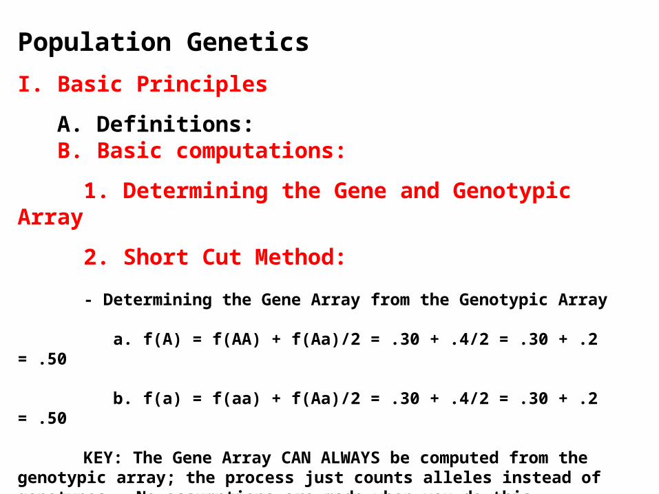
1. Determining the Gene and Genotypic Array
2. Short Cut Method:
- Determining the Gene Array from the Genotypic Array
a. f(A) = f(AA) + f(Aa)/2 = .30 + .4/2 = .30 + .2 = .50
b. f(a) = f(aa) + f(Aa)/2 = .30 + .4/2 = .30 + .2 = .50
KEY: The Gene Array CAN ALWAYS be computed from the genotypic array; the process just counts alleles instead of genotypes. No assumptions are made when you do this.

Population Genetics
I. Basic Principles
A. Definitions: B. Basic computations: C. Hardy-Weinberg Equilibrium:
1. If a population acts in a completely probabilistic manner, then: - we could calculate genotypic arrays from gene arrays - the gene and genotypic arrays would equilibrate in one generation
2. But for a population to do this, then the following assumptions must be met (Collectively called Panmixia = total mixing)
- Infinitely large (no deviation due to sampling error) - Random mating (to meet the basic tenet of random mixing) - No selection, migration, or mutation (gene frequencies must not
change)
Population GeneticsI. Basic Principles A. Definitions: B. Basic computations: C. Hardy-Weinberg Equilibrium:
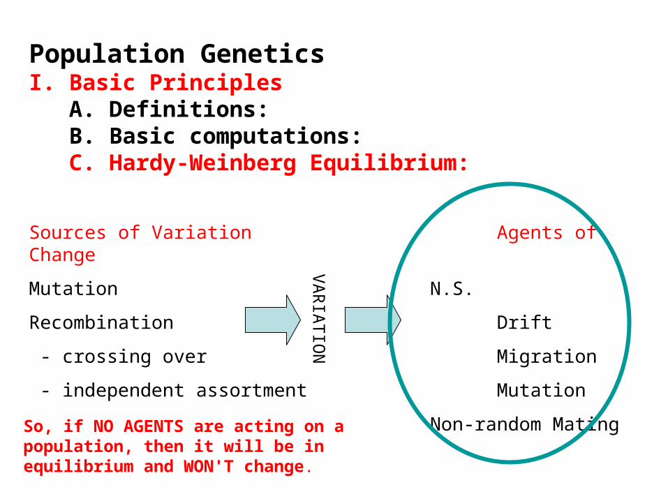
Sources of Variation Agents of Change
Mutation N.S.
Recombination Drift
- crossing over Migration
- independent assortment Mutation
Non-random Mating
VA
RIA
TIO
N
So, if NO AGENTS are acting on a population, then it will be in equilibrium and WON'T change.

Population Genetics
I. Basic Principles
A. Definitions: B. Basic computations: C. Hardy-Weinberg Equilibrium:
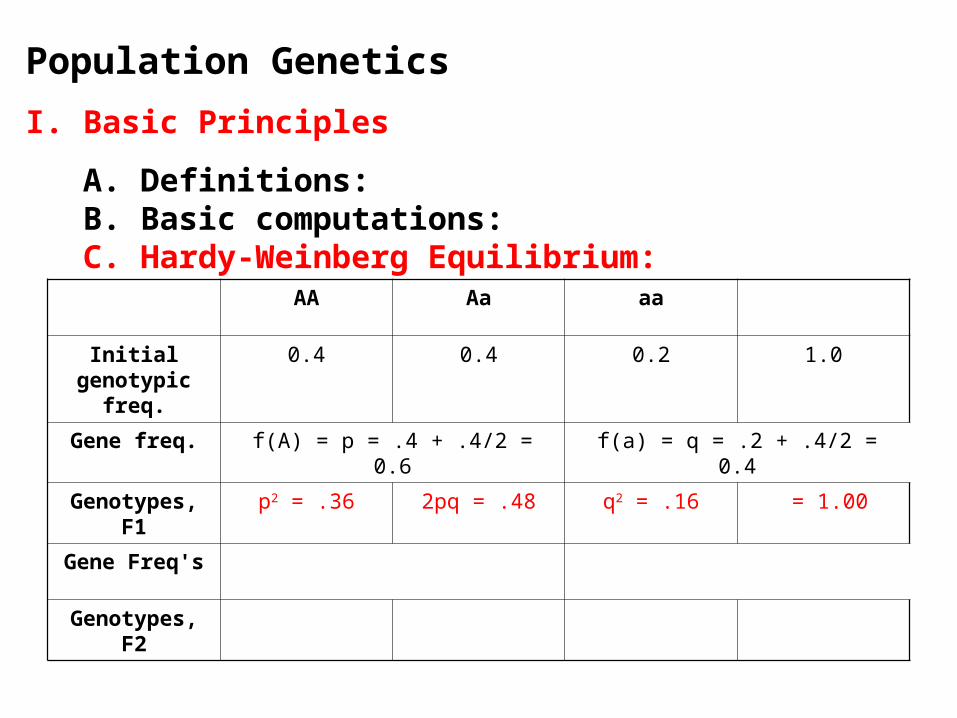
3. PROOF: - Given a population with p + q = 1. - If mating is random, then the AA, Aa and aa zygotes will be formed at p2 + 2pq + q2 - They will grow up and contribute genes to the next generation: - All of the gametes produced by AA individuals will be A, and they will be produced at a frequency of p2 - 1/2 of the gametes of Aa will be A, and thus this would be 1/2 (2pq) = pq - So, the frequecy of A gametes in the gametes will be p2 + pq = p(p + q) = p(1) = p - Likewise for the 'a' allele (remains at frequency of q). - Not matter what the gene frequencies, if panmixia occurs than the population will reach an equilibrium after one generation of random mating...

Population Genetics
I. Basic Principles
A. Definitions: B. Basic computations: C. Hardy-Weinberg Equilibrium:
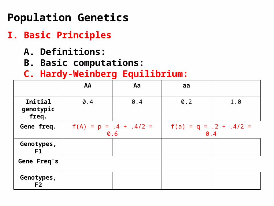
AA Aa aa
Initial genotypic freq.
0.4 0.4 0.2 1.0
Gene freq.
Genotypes, F1
Gene Freq's
Genotypes, F2
Population Genetics
I. Basic Principles
A. Definitions: B. Basic computations: C. Hardy-Weinberg Equilibrium:
AA Aa aa
Initial genotypic freq.
0.4 0.4 0.2 1.0
Gene freq. f(A) = p = .4 + .4/2 = 0.6 f(a) = q = .2 + .4/2 = 0.4
Genotypes, F1
Gene Freq's
Genotypes, F2
Population Genetics
I. Basic Principles
A. Definitions: B. Basic computations: C. Hardy-Weinberg Equilibrium:
AA Aa aa
Initial genotypic freq.
0.4 0.4 0.2 1.0
Gene freq. f(A) = p = .4 + .4/2 = 0.6 f(a) = q = .2 + .4/2 = 0.4
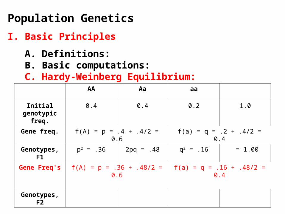
Genotypes, F1 p2 = .36 2pq = .48 q2 = .16 = 1.00
Gene Freq's
Genotypes, F2
Population Genetics
I. Basic Principles
A. Definitions: B. Basic computations: C. Hardy-Weinberg Equilibrium:
AA Aa aa
Initial genotypic freq.
0.4 0.4 0.2 1.0
Gene freq. f(A) = p = .4 + .4/2 = 0.6 f(a) = q = .2 + .4/2 = 0.4
Genotypes, F1 p2 = .36 2pq = .48 q2 = .16 = 1.00
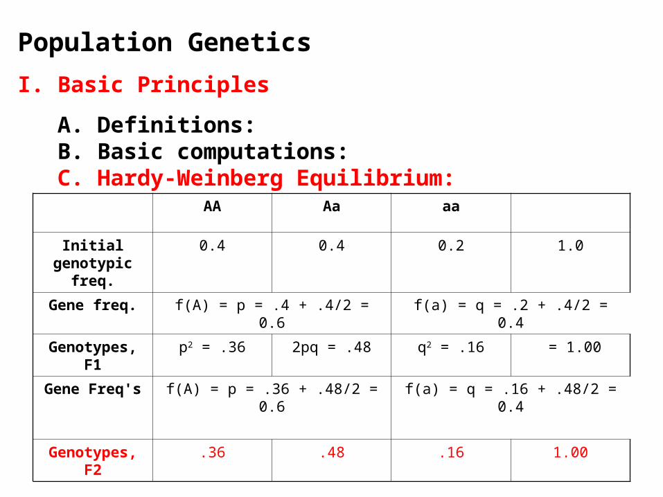
Gene Freq's f(A) = p = .36 + .48/2 = 0.6 f(a) = q = .16 + .48/2 = 0.4
Genotypes, F2
Population Genetics
I. Basic Principles
A. Definitions: B. Basic computations: C. Hardy-Weinberg Equilibrium:
AA Aa aa
Initial genotypic freq.
0.4 0.4 0.2 1.0
Gene freq. f(A) = p = .4 + .4/2 = 0.6 f(a) = q = .2 + .4/2 = 0.4
Genotypes, F1 p2 = .36 2pq = .48 q2 = .16 = 1.00
Gene Freq's f(A) = p = .36 + .48/2 = 0.6 f(a) = q = .16 + .48/2 = 0.4
Genotypes, F2 .36 .48 .16 1.00

Population Genetics
I. Basic Principles
A. Definitions: B. Basic computations: C. Hardy-Weinberg Equilibrium: D. Utility

Population Genetics
I. Basic Principles
A. Definitions: B. Basic computations: C. Hardy-Weinberg Equilibrium: D. Utility
1. If no real populations can explicitly meet these assumptions, how can the model be useful?

Population Genetics
I. Basic Principles
A. Definitions: B. Basic computations: C. Hardy-Weinberg Equilibrium: D. Utility
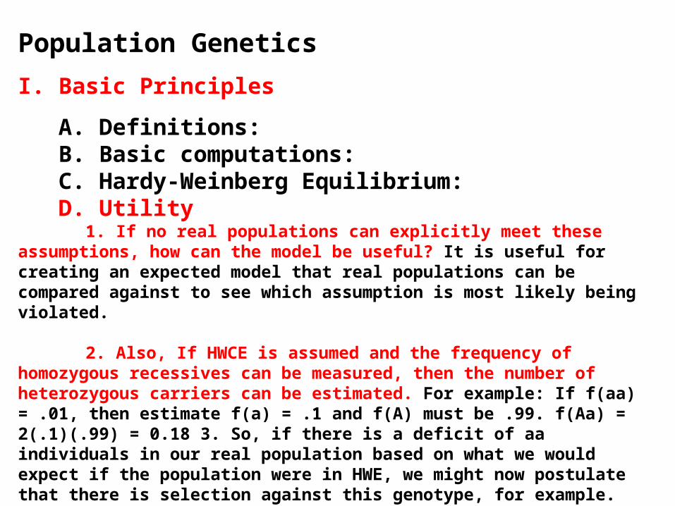
1. If no real populations can explicitly meet these assumptions, how can the model be useful? It is useful for creating an expected model that real populations can be compared against to see which assumption is most likely being violated.

Population Genetics
I. Basic Principles
A. Definitions: B. Basic computations: C. Hardy-Weinberg Equilibrium: D. Utility
1. If no real populations can explicitly meet these assumptions, how can the model be useful? It is useful for creating an expected model that real populations can be compared against to see which assumption is most likely being violated.
2. Also, If HWCE is assumed and the frequency of homozygous recessives can be measured, then the number of heterozygous carriers can
be estimated.
Population Genetics
I. Basic Principles
A. Definitions: B. Basic computations: C. Hardy-Weinberg Equilibrium: D. Utility
1. If no real populations can explicitly meet these assumptions, how can the model be useful? It is useful for creating an expected model that real populations can be compared against to see which assumption is most likely being violated.
2. Also, If HWCE is assumed and the frequency of homozygous recessives can be measured, then the number of heterozygous carriers can be estimated. For example: If f(aa) = .01, then estimate f(a) = .1 and f(A) must be .99. f(Aa) = 2(.1)(.99) = 0.18 3. So, if there is a deficit of aa individuals in our real population based on what we would expect if the population were in HWE, we might now postulate that there is selection against this genotype, for example.
Population Genetics
I. Basic Principles
A. Definitions: B. Basic computations: C. Hardy-Weinberg Equilibrium: D. Utility E. Extensions

Population Genetics
I. Basic Principles
A. Definitions: B. Basic computations: C. Hardy-Weinberg Equilibrium: D. Utility E. Extensions

Population Genetics
I. Basic Principles
A. Definitions: B. Basic computations: C. Hardy-Weinberg Equilibrium: D. Utility E. Extensions
1. 2 alleles in diploids: (p + q)2 = p2 + 2pq + q2

Population Genetics
I. Basic Principles
A. Definitions: B. Basic computations: C. Hardy-Weinberg Equilibrium: D. Utility E. Extensions
1. 2 alleles in diploids: (p + q)^2 = p^2 + 2pq + q^2
2. More than 2 alleles (p + q + r) 2 = p2 + 2pq + q2 + 2pr + 2qr + r2

Population Genetics
I. Basic Principles
A. Definitions: B. Basic computations: C. Hardy-Weinberg Equilibrium: D. Utility E. Extensions
1. 2 alleles in diploids: (p + q)^2 = p^2 + 2pq + q^2
2. More than 2 alleles (p + q + r)^2 = p^2 + 2pq + q^2 + 2pr + 2qr + r^2
3. Tetraploidy: (p + q)4 = p4 + 4p3q + 6p2q2 + 4pq3 + q4
(Pascal's triangle for constants...)

Population Genetics
I. Basic Principles
II. X-linked Genes

Population Genetics
I. Basic Principles
II. X-linked Genes A. Issue

Population Genetics
I. Basic Principles
II. X-linked Genes A. Issue
- Females (or the heterogametic sex) are diploid, but males are only haploid for sex linked genes.
Population Genetics
I. Basic Principles
II. X-linked Genes A. Issue
- Females (or the heterogametic sex) are diploid, but males are only haploid for sex linked genes.
- As a consequence, Females will carry 2/3 of these genes in a population, and males will only carry 1/3.

Population Genetics
I. Basic Principles
II. X-linked Genes A. Issue
- Females (or the heterogametic sex) are diploid, but males are only haploid for sex linked genes.
- As a consequence, Females will carry 2/3 of these genes in a population, and males will only carry 1/3.
- So, the equilibrium value will NOT be when the frequency of these alleles are the same in males and females... rather, the equilibrium will occur when: p(eq) = 2/3p(f) + 1/3p(m)
- Equilibrium will not occur with only one generation of random mating because of this imbalance... approach to equilibrium will only occur over time.
Population Genetics
I. Basic Principles
II. X-linked Genes
A. Issue B. Example
1. Calculating Gene Frequencies in next generation:
p(f)1 = ½[p(f)+p(m)] Think about it. Daughters are formed by an X from the mother and an X from the father. So, the frequency in daughters will be AVERAGE of the frequencies in the previous generation of mothers and fathers.

Population Genetics
I. Basic Principles
II. X-linked Genes
A. Issue B. Example
1. Calculating Gene Frequencies in next generation:
p(f)1 = 1/2(p(f)+p(m)) Think about it. Daughters are formed by an X from the mother and an X from the father. So, the frequency in daughters will be AVERAGE of the frequencies in the previous generation of mothers and fathers.
p(m)1 = p(f) Males get all their X chromosomes from their mother, so the frequency in males will equal the frequency in females in the preceeding generation.
Population Genetics
I. Basic Principles
II. X-linked Genes
A. Issue B. Example
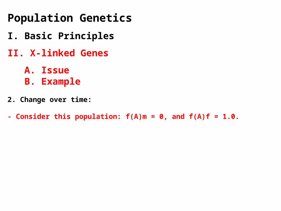
2. Change over time:
- Consider this population: f(A)m = 0, and f(A)f = 1.0.

Population Genetics
I. Basic Principles
II. X-linked Genes
A. Issue B. Example
2. Change over time:
- Consider this population: f(A)m = 0, and f(A)f = 1.0.
- In f1: p(m) = 1.0, p(f) = 0.5

Population Genetics
I. Basic Principles
II. X-linked Genes
A. Issue B. Example
2. Change over time:
- Consider this population: f(A)m = 0, and f(A)f = 1.0.
- In f1: p(m) = 1.0, p(f) = 0.5
- In f2: p(m) = 0.5, p(f) = 0.75

Population Genetics
I. Basic Principles
II. X-linked Genes
A. Issue B. Example
2. Change over time:
- Consider this population: f(A)m = 0, and f(A)f = 1.0.
- In f1: p(m) = 1.0, p(f) = 0.5
- In f2: p(m) = 0.5, p(f) = 0.75
- In f3: p(m) = 0.75, p(f) = 0.625
Population Genetics
I. Basic Principles
II. X-linked Genes
A. Issue B. Example
2. Change over time:
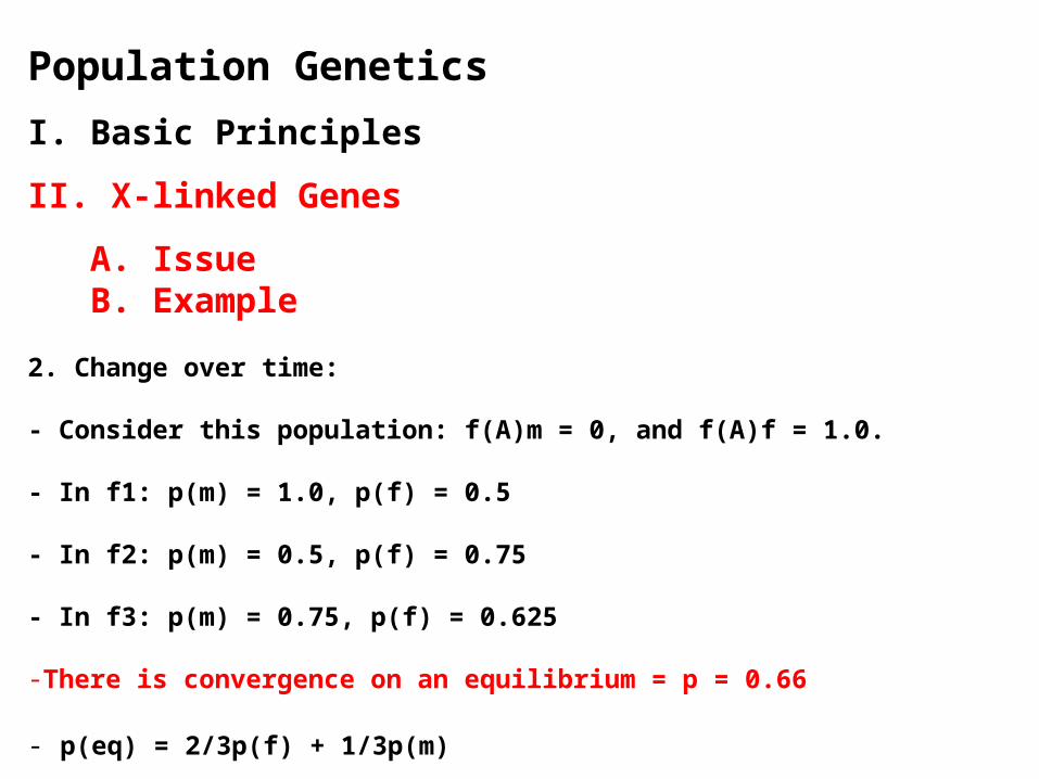
- Consider this population: f(A)m = 0, and f(A)f = 1.0.
- In f1: p(m) = 1.0, p(f) = 0.5
- In f2: p(m) = 0.5, p(f) = 0.75
- In f3: p(m) = 0.75, p(f) = 0.625
-There is convergence on an equilibrium = p = 0.66
- p(eq) = 2/3p(f) + 1/3p(m)
Population Genetics
I. Basic Principles
II. X-linked Genes
III. Modeling Selection
A. Selection for a Dominant Allele