I

POPULATION ECOLOGY OF BADGERS (TAXIDEA TAXUS) IN OHIO

A Thesis

Presented in Partial Fulfillment of the Requirements for

The Degree Master of Science in the

Graduate School of The Ohio State University

By

Jared F. Duquette, B.S.

The Ohio State University

2008

Master’s Examination Committee: Dr. Stanley D. Gehrt, Advisor Dr. Amanda Rodewald Dr. Darla Munroe Approved by __________________________________ Advisor Graduate Program in Natural Resources

ii

ABSTRACT

There is a paucity of information concerning American badger (Taxidea taxus)

ecology across the geographic range of this mesocarnivore. Virtually no research has

addressed the ecology of the badger east of the Mississippi River, particularly in a highly

fragmented agricultural landscape typical of this region. Therefore, I conducted a study

to assess certain aspects of badger ecology in areas dominated by agricultural use in Ohio

and west central Illinois.

I evaluated the state-wide badger distribution in Ohio through the collection of

badger observations using a state-wide publicity campaign. Overall, 387 badger

observations were collected: unconfirmed reports were most numerous (43%), followed

by probable (32%), and confirmed (25%). Relatively few observations were recorded

until the early 1990’s when they began to increase, and sharply increased during the 3-

year study period. Badgers were recorded in 56 counties, but most (>99%) of

observations were found in 53 counties above the glacial line.

I determined multi-scale spatial ecology and habitat use using radiotelemetry data

for badgers in Ohio (n = 5) and Illinois (n = 14) and an independent set of badger

observations in Ohio. Mean 95% FK annual home ranges in Illinois were larger than in

Ohio, but mean 50% FK annual home ranges did not differ between states. Mean 95%

FK annual home ranges for males were larger in Illinois than in Ohio; however, male

50% FK and both female annual home ranges did not differ between states. Both male

iii

home range sizes did not differ from females in Ohio, but 95% and 50% FK were larger

for males than females in Illinois over annual periods and during the rearing season; the

95% FK was also larger for males than females in Illinois during the breeding season.

Badgers in both states selected agricultural habitat within their home ranges, and linear

grassland and wetland-associated habitats within the study area landscape. Ohio badger

observations showed badger occurrence was associated with interspersed blocks of

agriculture and linear grassland habitats.

The spatially explicit habitat-relative abundance of badgers in Ohio was

determined through an independent set of badger observations and core home range

habitat use. Badger occurrence was associated with interspersed small blocks of

agriculture and linear grassland habitats. The model determined that 51% of the state

contained likely badger occurrence, 13% intermediate occurrence, and 36% unlikely

occurrence. The greatest likelihood of occurrence was mainly in the northwest,

southwest, and north central regions of the state. Predicted relative abundance was

relatively uniform in the northwest and north central regions of the state, with a uniform

pocket of likely occurrence in the south central region. The remainder of the state was

interspersed with likely to unlikely badger occurrence.

I evaluated population demography and diet through the collection and necropsy

of badger carcasses (n = 46) from 2005 to 2008. Diet data from 25 badgers showed small

mammals were predominately the main prey items. Mean age of 38 badgers was 1.63

years and categorically consisted of 34% young-of-year, 16% sub-adults, and 50% adults.

Fecundity was estimated as 0.302 with a mean litter size of 2.17 and 31.6% occurrence of

parous females, which included 2 known age young-of-year. The base population model

iv

with a starting population of 500 females increased (λ = 1.032) gradually after 20 years.

Badger young-of-year survival appeared to be an important factor for influencing

population growth rate, as lower estimates caused substantial population declines over a

20-year time period. A simulated 4.5% population harvest also showed sharp population

declines over the same period.

Deforestation and agricultural practices have likely allowed the population

expansion of badgers into areas of the state beyond the historical distribution that was

presumably restricted to prairie pockets of the state. The spatial ecology of badgers in

agricultural landscapes appears to be contingent on the habitat composition in the

respective landscape. Badgers use the landscape at multiple spatial scales and

management of grassland habitats and riparian corridors appear to be important to the

conservation of this species. In addition, the future trend of this low-density population is

highly dependent on the survival and reproduction of female badgers, particularly

younger animals.

v

ACKNOWLEDGMENTS

First and foremost I would like to thank my friends and family for supporting me

in all of my endeavors, particularly throughout this project. Secondly, I would like to

graciously thank my advisor Stan Gehrt for giving me a chance to conduct this

spectacular study and to whom I am greatly indebted for his contributions to this project.

Commendation is given to my committee members Amanda Rodewald and Darla

Munroe for their guidance and insights throughout the study. This project would not

have been possible without the funding and support of the Ohio Division of Wildlife and

associated employees. A huge thank you goes to Joe Barber for his willingness to fly all

over Ohio at the drop of a hat in order to radiotrack my animals. There is a long list of

additional natural resource and wildlife related offices and individuals I would like to

recognize, however, for sake of space those entities received my personal recognition.

I greatly appreciate the assistance of Drs. Thomas Gehring and Kurt Ver Cauteren

in helping me achieve my goals and being great role models. Furthermore, this study

would not have been possible without the great cooperation from the citizens of Ohio,

particularly members of the fur harvest community. Gratitude is also extended to the

Indiana Department of Natural Resources, above all Scott Johnson, for their cooperation

in this study. Additionally, the cooperation of Barbara Ver Steeg, Richard Warner,

Marsha Sovada, and John Messick is deeply appreciated. Finally, I need to distinguish

those individuals who have pushed me along the way to be the best I can, rest in peace

vi

VITA

August 2005 – August 2008 ..............Graduate Research Associate, The Ohio State University, Columbus, Ohio May 2004 – September 2005 .............Wildlife Technician USDA/APHIS/WS/NWRC, Fort Collins, Colorado September 2004 – September 2005 ...Wildlife Technician Central Michigan University August 2000 – May 2004...................B.S. Biology with Minor: Psychology, Central

Michigan University, Mount Pleasant, Michigan

FIELDS OF STUDY

Major Field: Natural Resources

vii

TABLE OF CONTENTS

ABSTRACT........................................................................................................................ ii ACKNOWLEDGMENTS .................................................................................................. v VITA.................................................................................................................................. vi LIST OF APPENDICES.................................................................................................... ix LIST OF TABLES............................................................................................................. xi LIST OF FIGURES ......................................................................................................... xiii Chapters: 1. DISTRIBUTION OF THE BADGER (TAXIDEA TAXUS) IN OHIO…………. 1

1.1 INTRODUCTION……………………………………………………………. 1 1.2 METHODS…………………………………………………………………… 5

1.2.1 Study area………………………………………………………………. 5 1.2.2 Observation data………………………………………………………... 5 1.2.3 Observation collection………………………………………………….. 6

1.3 RESULTS…………………………………………………………………….. 8 1.4 DISCUSSION………………………………………………………………... 8 1.5 LITERATURE CITED………………………………………………………. 13

2. SPATIAL ECOLOGY AND HABITAT USE OF BADGERS (TAXIDEA TAXUS) IN AGRICULTURAL LANDSCAPES………………….. 21

2.1 INTRODUCTION……………………………………………………………. 21 2.2 METHODS…………………………………………………………………… 25

2.2.1 Study area………………………………………………………………. 25 2.2.2 Capture and Radiotelemetry……………………………………………. 26 2.2.3 Landscape data…………………………………………………………. 28 2.2.4 Home range estimation…………………………………………………. 29 2.2.5 2nd order habitat and patch structure selection………………………….. 30 2.2.6 3rd order habitat selection………………………………………………. 33 2.2.7 Ohio landscape scale analysis…………………………………………... 33

2.3 RESULTS…………………………………………………………………….. 37

2.3.1 Home range estimation…………………………………………………. 37

viii

2.3.2 2nd order habitat and patch structure selection………………………….. 38 2.3.3 3rd order habitat selection………………………………………………. 39 2.3.4 Ohio landscape scale analysis…………………………………………... 40

2.4 DISCUSSION………………………………………………………………... 41 2.5 LITERATURE CITED………………………………………………………. 49

3. BADGER (TAXIDEA TAXUS) HABITAT-RELATIVE ABUNDANCE I N OHIO……………………………………………………………………………... 64

3.1 INTRODUCTION……………………………………………………………. 64 3.2 METHODS…………………………………………………………………… 67

3.2.1 Study area………………………………………………………………. 67 3.2.2 Badger observations……………………………………………………. 67 3.2.3 Landscape data…………………………………………………………. 68 3.2.4 Habitat variable selection………………………………………………. 68 3.2.5 Abundance estimation………………………………………………….. 71 3.2.6 Model classification…………………………………………………….. 72

3.3 RESULTS…………………………………………………………………….. 72 3.4 DISCUSSION………………………………………………………………... 74 3.5 LITERATURE CITED………………………………………………………. 77

4. POPULATION DEMOGRAPHY AND DIET OF BADGERS (TAXIDEA TAXUS) IN OHIO………………………………………………….. 83

4.1 INTRODUCTION……………………………………………………………. 83 4.2 METHODS…………………………………………………………………… 89

4.2.1 Carcass collection and necropsy……...………………………………... 89 4.2.2 Diet composition……...………………………………………………... 89 4.2.3 Sex……………………………………………………………………. 90 4.2.4 Age structure…………………………………………………………. 90 4.2.5 Morphometrics……………………...………………………………... 90 4.2.6 Reproductive status………………...………………………………… 91 4.2.7 Population modeling……...………………………………………….. 92

4.3 RESULTS…………………………………………………………………… 94

4.3.1 Age structure…………………………………………………………... 94 4.3.2 Morphometrics………………………………………………………… 94 4.3.3 Diet composition……………………………………………………… 95 4.3.4 Population models…………………………………………………….. 95

ix

4.4 DISCUSSION………………………………………………………………. 97 4.5 LITERATURE CITED……………………………………………………… 106

BIBLIOGRAPHY…………………………………………………………………… 119

Appendix A. Badger observation poster, originally 11” X 14”, used to opportunistically collect badger reports in Ohio from 2005-2008. Lower left corner of poster shows image of pre-paid tear-off cards placed on posters which allowed observers to send in their report…………………………………………………………………………………....129 Appendix B. Fur harvester inquiry used in 2006 to obtain reports of badger observations and captures in Ohio……………………………………………………………………130 Appendix C. Reclassification scheme of Ohio GAP land cover data……..…………...131 Appendix D. Reclassification scheme of Illinois GAP land cover data.........................132 Appendix E. Sex, age class, and fate of radioharnessed badgers in Ohio study from 2005-2007………………………………………………………………………………133 Appendix F. Annual home range estimates for individual badgers in Ohio from 2005 to 2007. Badger sex, age class, radiolocations (Locations), 100% minimum convex polygon (100 MCP) home range, 95% fixed kernel (95 FK) home range, and 50% (50 FK) home range are reported………………………...…………………………………………….134 Appendix G. Sex, age class, and fate of radioimplanted badgers in Illinois study from 1990-1995………………………………………………………………………………135 Appendix H. Annual home range estimates for individual badgers in Illinois from 1990 to 1995. Badger sex, age class, radiolocations (Locations), 100% minimumconvex polygon (100 MCP) home range, 95% fixed kernel (95 FK) home range, and 50% (50 FK) home range………………………………………………………..………….........138 Appendix I. Seasonal home range estimates for individual badgers in Ohio from 2005 to 2007. Badger sex, age class, radiolocations (Locations), 100% minimum convex polygon (100 MCP) home range, 95% fixed kernel (95 FK) home range, and 50 % (50 FK) home range……………………………….………………………..…………………………..139 Appendix J. Seasonal home range estimates for individual badgers in Illinois from 1990 to 1995. Badger sex, age class, radiolocations (Locations), 100% minimum convex polygon (100 MCP) home range, 95% fixed kernel (95 FK) home range, and 50% (50 FK) home range…………………………………...........................................................140

x

Appendix K. Badger carcass identification, date collected, county of collection, sex, age (years), cause of mortality, evidence of reproduction, baculum length (mm), and baculum weight (g). Carcasses collected in Ohio during 2005-2008. Reproduction indicated as present (Y) or not present (N) and type of reproductive evidence is indicated by a lactation, b blastocysts, or c placental scars……………………………………………...142 Appendix L. Skull measurements for male (n = 7) and female (n = 7) badgers collected during 2005-2008 in Ohio……………………………………………………………...144

xi

LIST OF TABLES

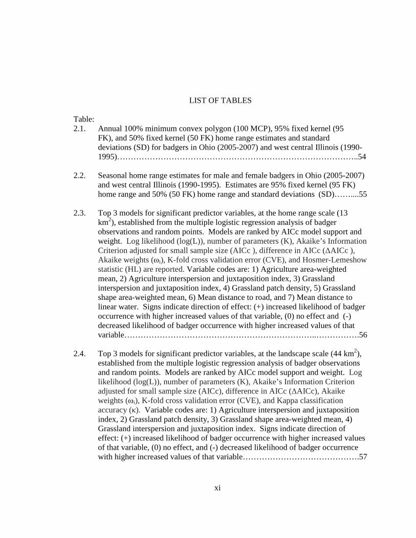
Table: 2.1. Annual 100% minimum convex polygon (100 MCP), 95% fixed kernel (95 FK), and 50% fixed kernel (50 FK) home range estimates and standard deviations (SD) for badgers in Ohio (2005-2007) and west central Illinois (1990- 1995)……………………………………………………………………………..54 2.2. Seasonal home range estimates for male and female badgers in Ohio (2005-2007) and west central Illinois (1990-1995). Estimates are 95% fixed kernel (95 FK) home range and 50% (50 FK) home range and standard deviations (SD)……....55 2.3. Top 3 models for significant predictor variables, at the home range scale (13 km2), established from the multiple logistic regression analysis of badger observations and random points. Models are ranked by AICc model support and weight. Log likelihood (log(L)), number of parameters (K), Akaike’s Information Criterion adjusted for small sample size (AICc ), difference in AICc (∆AICc ), Akaike weights (ωi), K-fold cross validation error (CVE), and Hosmer-Lemeshow statistic (HL) are reported. Variable codes are: 1) Agriculture area-weighted mean, 2) Agriculture interspersion and juxtaposition index, 3) Grassland interspersion and juxtaposition index, 4) Grassland patch density, 5) Grassland shape area-weighted mean, 6) Mean distance to road, and 7) Mean distance to linear water. Signs indicate direction of effect: (+) increased likelihood of badger occurrence with higher increased values of that variable, (0) no effect and (-) decreased likelihood of badger occurrence with higher increased values of that variable……………………………………………………………..…………….56 2.4. Top 3 models for significant predictor variables, at the landscape scale (44 km2), established from the multiple logistic regression analysis of badger observations and random points. Models are ranked by AICc model support and weight. Log likelihood (log(L)), number of parameters (K), Akaike’s Information Criterion adjusted for small sample size (AICc), difference in AICc (∆AICc), Akaike weights (ωi), K-fold cross validation error (CVE), and Kappa classification accuracy (κ). Variable codes are: 1) Agriculture interspersion and juxtaposition index, 2) Grassland patch density, 3) Grassland shape area-weighted mean, 4) Grassland interspersion and juxtaposition index. Signs indicate direction of effect: (+) increased likelihood of badger occurrence with higher increased values of that variable, (0) no effect, and (-) decreased likelihood of badger occurrence with higher increased values of that variable…………………………………….57

xii

3.1. Mean values (± SE) of 7 habitat variables used to model badger habitat in Ohio and correlations between each variable and Penrose distance (PD). a Significant (P ≤0.05) correlations are denoted as (S)………………………………………..79 4.1. Population parameters used to model the Ohio badger population. a A mean estimate of young-of-year survival. b A maximum estimate of young-of-year survival………………………………………………………………………….110 4.2. Ages (in years) for male, female, and sex unknown badgers collected during 2005-2008 in Ohio……………………………………………………………...111 4.3. Age class, cause of mortality, and number of badger carcasses collected during 2005-2008 in Ohio……………………………………………………………...112 4.4. Morphometrics for male and female badgers by age class collected during 2005- 2008 in Ohio………………………………………………………………...….113 4.5. Diet composition of badger carcass gastrointestinal contents (n = 25) collected during 2005-2008 in Ohio………………………………………………………114

xiii

LIST OF FIGURES

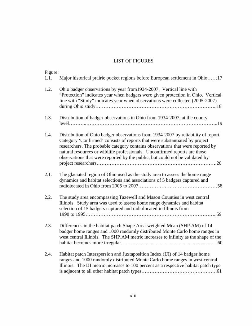
Figure: 1.1. Major historical prairie pocket regions before European settlement in Ohio……17 1.2. Ohio badger observations by year from1934-2007. Vertical line with “Protection” indicates year when badgers were given protection in Ohio. Vertical line with “Study” indicates year when observations were collected (2005-2007) during Ohio study………………………………………………………………..18 1.3. Distribution of badger observations in Ohio from 1934-2007, at the county level………..……………………………………………………………………..19 1.4. Distribution of Ohio badger observations from 1934-2007 by reliability of report. Category ‘Confirmed’ consists of reports that were substantiated by project researchers. The probable category contains observations that were reported by natural resources or wildlife professionals. Unconfirmed reports are those observations that were reported by the public, but could not be validated by project researchers……………………………………………………………….20 2.1. The glaciated region of Ohio used as the study area to assess the home range dynamics and habitat selections and associations of 5 badgers captured and radiolocated in Ohio from 2005 to 2007…………………………………………58 2.2. The study area encompassing Tazewell and Mason Counties in west central Illinois. Study area was used to assess home range dynamics and habitat selection of 15 badgers captured and radiolocated in Illinois from 1990 to 1995……………………………………………………………………..59 2.3. Differences in the habitat patch Shape Area-weighted Mean (SHP.AM) of 14 badger home ranges and 1000 randomly distributed Monte Carlo home ranges in west central Illinois. The SHP.AM metric increases to infinity as the shape of the habitat becomes more irregular…………………………………………………..60 2.4. Habitat patch Interspersion and Juxtaposition Index (IJI) of 14 badger home ranges and 1000 randomly distributed Monte Carlo home ranges in west central Illinois. The IJI metric increases to 100 percent as a respective habitat patch type is adjacent to all other habitat patch types……………………………………….61

xiv

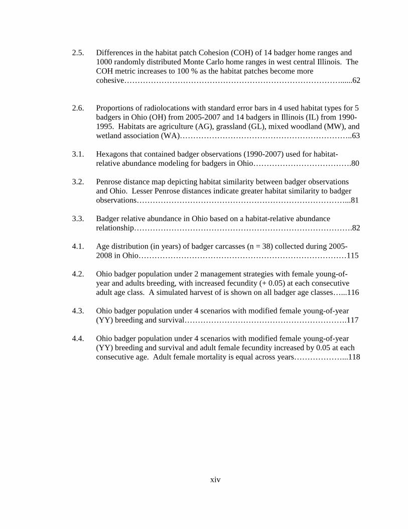
2.5. Differences in the habitat patch Cohesion (COH) of 14 badger home ranges and 1000 randomly distributed Monte Carlo home ranges in west central Illinois. The COH metric increases to 100 % as the habitat patches become more cohesive………………………………………………………………………......62 2.6. Proportions of radiolocations with standard error bars in 4 used habitat types for 5 badgers in Ohio (OH) from 2005-2007 and 14 badgers in Illinois (IL) from 1990- 1995. Habitats are agriculture (AG), grassland (GL), mixed woodland (MW), and wetland association (WA)………………………………………………………..63 3.1. Hexagons that contained badger observations (1990-2007) used for habitat- relative abundance modeling for badgers in Ohio……………………………….80 3.2. Penrose distance map depicting habitat similarity between badger observations and Ohio. Lesser Penrose distances indicate greater habitat similarity to badger observations……………………………………………………………………...81 3.3. Badger relative abundance in Ohio based on a habitat-relative abundance relationship……………………………………………………………………….82 4.1. Age distribution (in years) of badger carcasses (n = 38) collected during 2005- 2008 in Ohio……………………………………………………………………115 4.2. Ohio badger population under 2 management strategies with female young-of- year and adults breeding, with increased fecundity (+ 0.05) at each consecutive adult age class. A simulated harvest of is shown on all badger age classes…...116 4.3. Ohio badger population under 4 scenarios with modified female young-of-year (YY) breeding and survival…………………………………………………….117 4.4. Ohio badger population under 4 scenarios with modified female young-of-year (YY) breeding and survival and adult female fecundity increased by 0.05 at each consecutive age. Adult female mortality is equal across years………………...118

1

CHAPTER 1

DISTRIBUTION OF THE BADGER (TAXIDEA TAXUS) IN OHIO

INTRODUCTION

Investigating the spatial distribution of a population, monitoring spatiotemporal

trends, and understanding factors that influence these trends can provide essential

information for a species adaptive conservation strategy (Apps et al. 2004). Knowledge

of species distribution and relationship to environmental variables can also help provide

detailed information for the management of biodiversity, species protection, species

reintroduction, and prediction of possible impacts of land use or climate change (Aspinall

et al. 1998). The distribution of a species is partially determined from the physical and

biotic variables found in the environment, and therefore distribution is not commonly

uniform (Warrick and Cypher 1998). Environmental variables (e.g. road density and

prey abundance) play direct and indirect roles in determining the distribution of many

mammalian carnivores, such as the bobcat Lynx rufus (Wolff et al. 2002), which

frequently do not possess a uniform distribution. Environmental changes have caused

some mammalian carnivore species (e.g. coyote Canis latrans) to expand their range,

whereas some have been greatly reduced (e.g. grey wolf Canis lupus) (Ray 2000).

2

Range fluctuations have resulted from many environmental pressures (e.g. climate

change); however anthropogenic habitat modification has played an immense role in

determining the present range of many mammalian carnivores. Mammalian carnivores

are commonly considered sensitive indicators of environmental change (Zielinski et al.

2005) and therefore may serve as umbrella species to assess habitat suitability for many

species not found in this guild.

Because mammalian carnivore populations can be greatly affected by

anthropogenic land use, knowledge of their range contractions and expansions, and

underlying causes, is important for future conservation efforts (Laliberte and Ripple

2004). Comparing the contemporary and historical distributions of populations and

habitats can lead to knowledge about the population status of wildlife species (Zielinski

et al. 2005). If this comparison spans a time over which humans have had significant

influences on habitat or populations, then it can allow an understanding of the effects of

anthropogenic change on populations. This comparison is particularly useful for

grassland carnivores as they have direct and indirect effects on vertebrate community

structure (Crooks 2002, Zielinski et al. 2005).

The temperate grassland biome has lost more species than any other North

American biome and prairies have declined by an average of 79% since the early 1800’s

(Laliberte and Ripple 2004). This loss has affected the native range of grassland species

in different ways and major range contractions have been documented in swift fox

(Vulpes velox; Kamler et al. 2003), black footed prairie dogs (Cynomys ludovicianus;

Daley 1992), lesser prairie chickens (Tympanuchus pallidicinctus; Fuhlendorf et al.

2002), and bison (Bison bison; Freese et al. 2007), while coyotes (Canis latrans) have

3

greatly expanded their range (Gosselink et al. 2007). Differences in range dynamics have

largely resulted from the critical habitat requirements of each species, with habitat

generalists such as the coyote more able to adapt to landscape fragmentation and

conversion to agriculture (Kamler et al. 2003). Similar to the coyote, the American

badger (Taxidea taxus) is another grassland associated carnivore thought to have

experienced a range expansion due to anthropogenic land use practices.

The badger is a fossorial mesocarnivore native to North American grassland

habitats and is considered an important indicator of the quantity and quality of prairies

(Warner and Ver Steeg 1995). The badger has experienced an estimated geographic

range increase of 17% from the species’ historical range (Laliberte and Ripple 2004).

The historical distribution of the badger is considered the western and north central

United States and south central Mexico, with populations extending into British

Columbia and across Ontario (Hoodicoff 2003, Lintack and Voigt 1983). However,

several authors have reported increased badger occurrence in less abundant areas such as

southeast Kansas (Cleveland 1985), southeast Oklahoma (Tumlison and Bastarache

2007), northern Minnesota (Jannett et al. 2007), eastern Indiana (Lyon 1932, Berkley and

Johnson 1998), and across Illinois (Gremillion-Smith 1985, Warner and Ver Steeg 1995).

Moreover, several authors have proposed an extended badger range expansion in Ohio,

the presumed eastern extent of their distribution (Moseley 1934, Nugent and Choate

1970, Leedy 1947, Berkley and Johnson 1998).

Although badger range expansion has been documented in several states east of

the Mississippi River, the statewide population status and distribution of the badger is

unknown in Ohio. Historically, badgers have been presumed to be rare in Ohio (Smith et

4

al. 1973). The rare nature and unknown population status of the badger led the Ohio

Division of Wildlife (ODOW) to fully protect the badger state-wide as a Species of

Concern in 1990. Badgers are a native species to Ohio and presumably endemic to the

historical prairie regions of the state (Moseley 1934), but the influence of anthropogenic

land use on the distribution of this population is virtually unknown.

Before European settlement, land cover in Ohio was approximately 95% forested

(Gordon 1966), but deforestation practices, largely for agriculture, during the early 19th

century reduced the forest cover to roughly 10% (Ohio Division of Forestry 2008). Land

clearance gave way to a fragmented landscape matrix of primarily agriculture, possibly

providing greater suitable habitat for badgers such as hedgerows and pastures. In

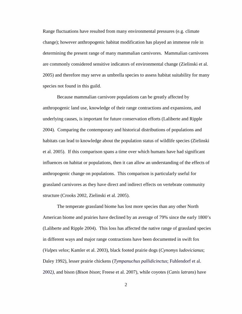
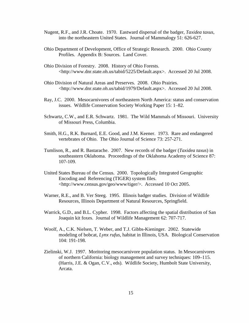
addition, pre-settlement Ohio contained 3 main native prairie pocket regions, including

the Oak Opening and Sandusky Plains in the northwest region and Darby Plains in the

west central region of the state (Figure 1.1). Historical accounts suggest that native

badger populations may have persisted in these regions prior to the ensuing deforestation

(Hine 1906, Moseley 1934). Successive deforestation around these existing prairie

populations, commonly converted to agriculture, may have additionally provided badgers

increased habitat and travel corridors allowing for potential population expansion.

Although badgers are considered uncommon in Ohio, a proportionally greater

number of observation reports have been reported to the ODOW in the past decade

compared to years past. The factors attributed to these increased observation reports are

unknown. However, assessing the spatial distribution of these observations may provide

insights into factors that have potentially led to these increased reports. In addition, the

assessment badger observations over time can provide a means to record changes in

5

distribution over a state-wide scale. This approach has been used as a form of monitoring

for species that are rare on the basis of abundance because these species are usually also

rare on the basis of geographic distribution (Gaston and Lawton 1990, Zielinski 1997).

With these considerations the following objectives were to: 1) determine the distribution

of the badger in Ohio based on reported badger observations, and 2) evaluate the status of

the badger in Ohio based on the abundance of observations and overall distribution.

METHODS

Study Area

The study encompassed all 88 counties in Ohio, from 38° 24‘N to 41° 59‘N and

80° 32° W to 84° 49° W. State-wide land cover was approximately 60% agriculture,

35% woodland/shrub, 3% urban, <1% open water, <1% wetland, and <1% barren (Ohio

Department of Development 2000). The glaciated central, western, and northwestern

regions of the state were characterized by a highly fragmented matrix of agriculture, with

minimal topographical variation. The remainder of the state was largely interspersed

with forest and agriculture, but was predominantly forested in the southeastern region.

The geology and associated landscape largely changed from glaciated alluvial soils to

unglaciated soils of sandstone and shale as defined by the Wisconsinan glacial line. The

glaciated region covered approximately 66% of the state and the unglaciated

approximately 34%. Elevations gradually decreased from north to south and range from

472 m to 139 m.

Observation Data

For each badger observation I attempted to gather detailed information on the

observation location, date, observer name and contact information, associated observer

6

comments, and a Geographic Positioning System (GPS) coordinate if available. I

classified each observation for validity based on the evidence provided from the

information and my personal contact with observer(s).

Observation Collection

As badgers are presumed to be uncommon in the state, I actively and

opportunistically collected observation data using multiple methods from January 2005 to

January 2008. Active collection methods included informational presentations,

observation posters, and a fur harvester mail inquiry. I also made efforts to glean records

of badgers from extant scientific literature and other historical records from museum

specimens and the Ohio Natural Heritage database.

Over the course of the study 204 large posters (Appendix A) describing basic

badger characteristics and ecology were sent out to pertinent wildlife and natural resource

related offices and the Ohio Department of Transportation (ODOT) offices, respectively.

These posters included tear-off badger observation report cards that provided pre-paid

postage that were addressed directly to researchers. These posters were modified from

designs successfully used by Warner and Ver Steeg (1995) in Illinois and John Messick

(pers. comm.) in Missouri. Badger images were obtained by permission from Schwartz

and Schwartz (1981). In addition, smaller versions of these posters, without report cards,

were placed opportunistically at locations where the public would commonly view these

postings (e.g. fueling stations).

Throughout the study, several forms of mass media were used to gather public

observations. In the winter of 2006 an informational badger web page was designed in

collaboration with ODOW staff. This web page contained a navigation link to an

7

additional web page where persons could report badger observations to researchers.

Furthermore, I published numerous informational columns in several Ohio popular media

and gave presentations explaining the study and requesting badger observations at

wildlife agency workshops and conferences and applicable public and private interest

gatherings.

In addition, a fur harvester mail inquiry was distributed to 1,500 randomly-

selected individuals during the last week of February 2006 (Appendix B). This inquiry

was directed at individuals who stated they would harvest furbearers in the 2005-2006

season, as these persons are commonly outdoors and possibly have an increased

probability of identifying and observing badgers. The inquiry was intended to gather

both first and second hand badger observations and the associated date, type of sign, and

status (dead or alive) of badger. All collected badger observations were classified into 1

of 3 classifications based on the strength of the evidence: confirmed (e.g. definitive

evidence like a road-kill or photograph), probable (observations from wildlife-related

professionals), or unconfirmed (public report, not positively confirmed).

To determine the state-wide distribution of the badger, I used a Geographic

Information System (GIS) to map collected badger observations on a county scale. A

Topologically Integrated Geographic Encoding and Referencing (TIGER) system county

boundary files (United States Bureau of the Census 2000) were obtained for Ohio. I then

joined pertinent observation data tables with the Ohio TIGER file table using respective

Ohio counties as the join field. Finally, I used the symbology tool to classify and display

the number of badger observations per county and badger observations by validity

classification. ArcGIS 9.1 (ESRI 2005) was used for all geospatial analyses.

8

RESULTS

I obtained 387 badger observations, of which unconfirmed reports being most

numerous (43%), followed by probable (32%), and confirmed (25%). Observation

records were obtained from the following sources: report cards (7%), ODOW website

(7%), fur harvest inquiry (19%), trapped (4%), carcasses (10%), historical records (5%),

creditable sources (19%), and public relations (29%). Observation reports from popular

media and presentations were most common (29%), followed by reports from creditable

wildlife-related professionals (19%).

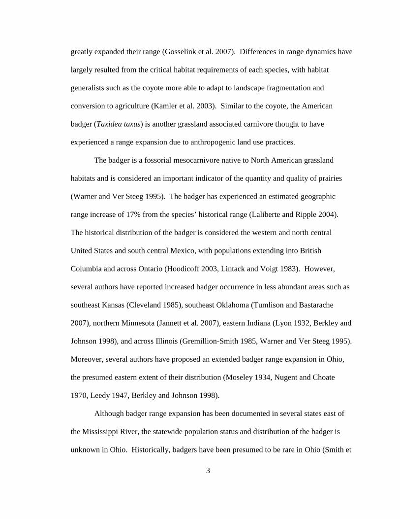
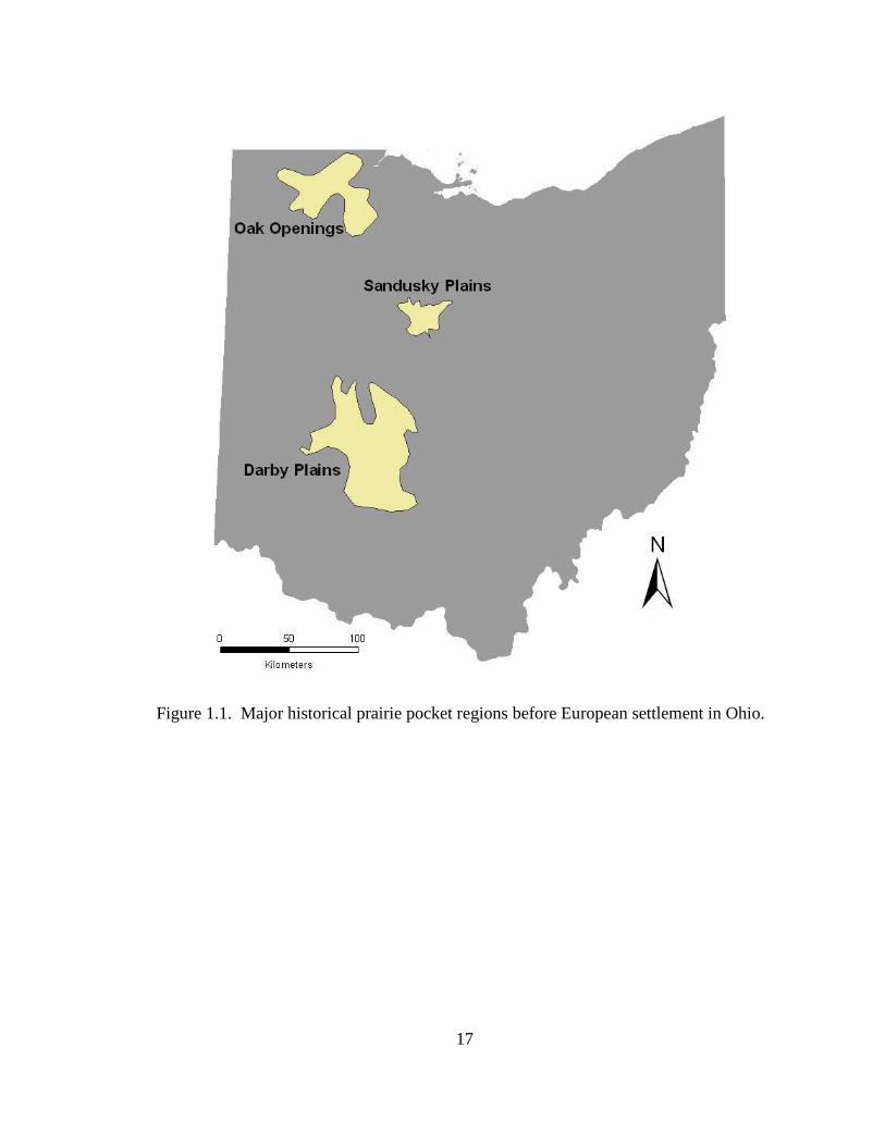
The number of observations was consistently low until the early 1990’s when they

began to gradually increase and sharply increased during the 3-year study period (Figure

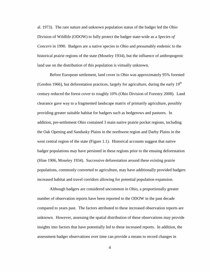
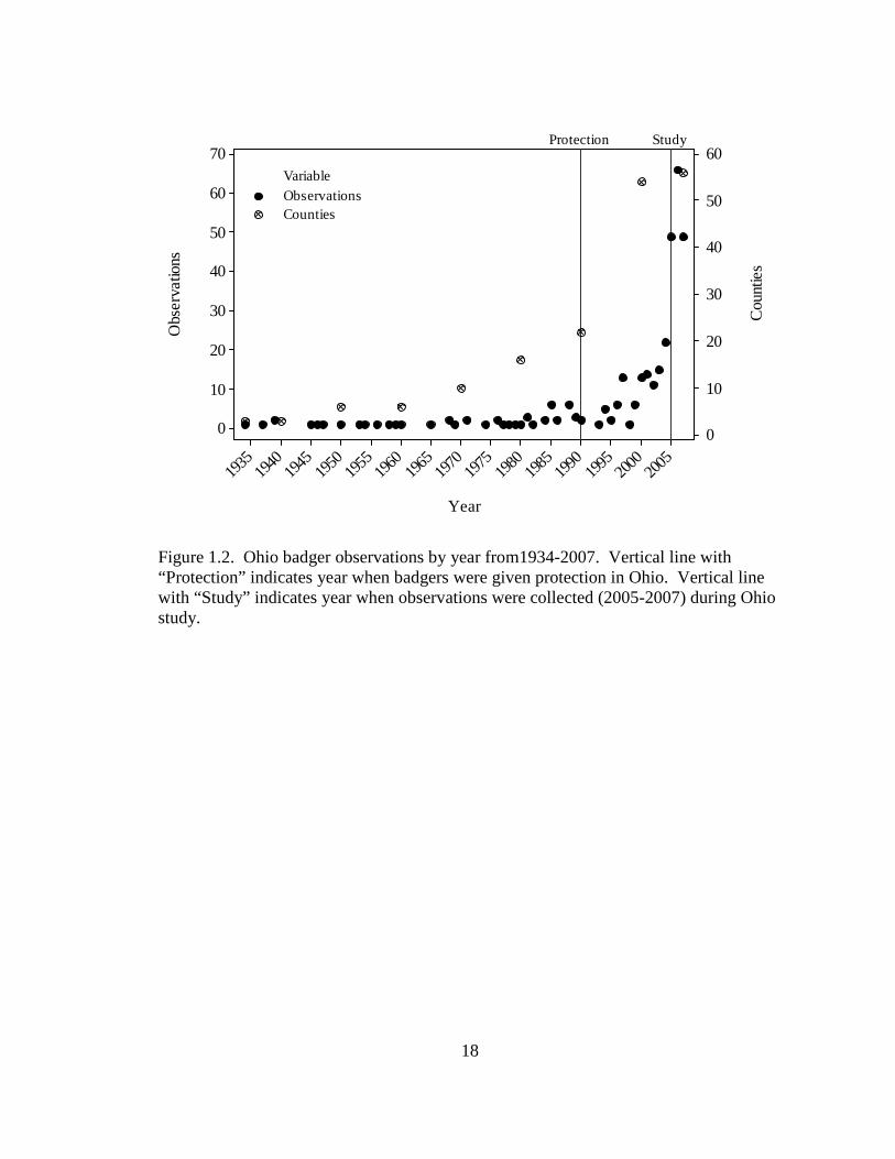
1.2). Badgers were recorded in 56 counties, but were found in 53 counties above the

glacial line accounting for >99% of all observations and 3 counties below the glacial line

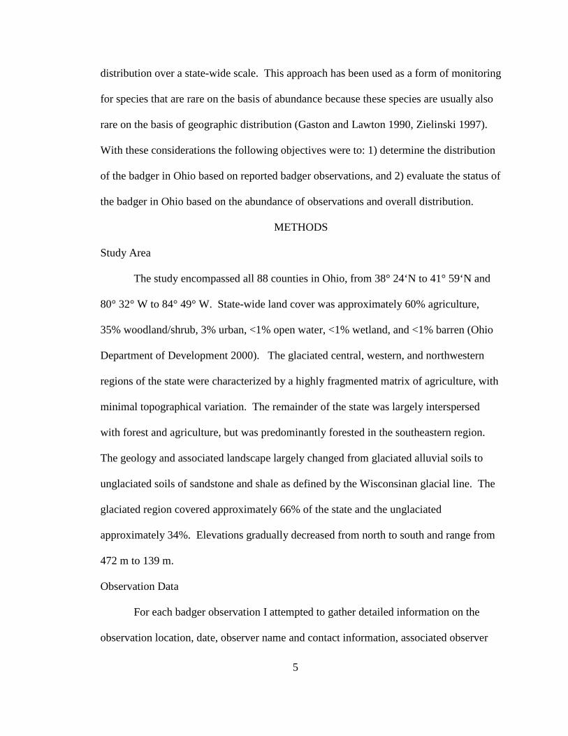
accounting for <1% of all observations (Figure 1.3). Evidence of badgers was confirmed

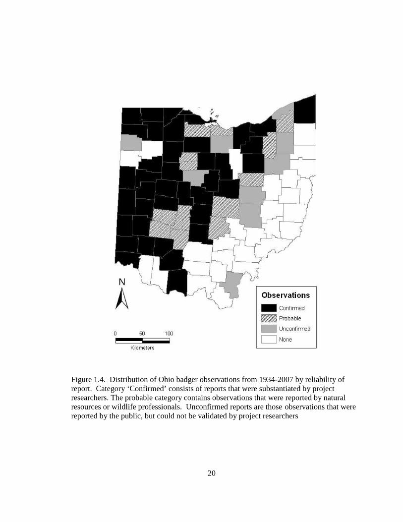
in 39 counties, probable in 37 counties, and unconfirmed in 52 counties (Figure 1.4).

Prior to the state-wide protection of the badger in 1990, badgers were observed in only 22

counties, but increased to 56 counties thereafter (Figure 1.2). The 4 counties with the

highest number of observations were located in the northwest and west central regions of

the state (Figure 1.3) and accounted for approximately 26% of all observations.

DISCUSSION

Overall distribution records occurred in nearly every county in the glaciated

region of the state. This constitutes an extensive range expansion for the badger in Ohio

compared to their presumed historical distribution in the native prairie pockets found in

the northwest and central regions of the state. Although, counties with the highest

9

number of recorded observations remained in the historical prairie pocket regions. The

core areas of the badger distribution in Ohio appear to be centered on the historical

prairie regions of the state. These areas still nurture prairie remnants and friable soils that

may likely provide badgers with the greatest amount of suitable habitat in the state. From

these historical regions, the population appears to have expanded into numerous counties

found in the northeast and southern regions of the state. However, only 3 badger

observations were recorded below the glacial line and further range expansion may be

largely limited by the flora and soil change in the unglaciated region.

Similar range expansions have been documented by other studies in the

Midwestern states of Illinois (Gremillion-Smith 1985, Warner and Ver Steeg 1995) and

Indiana (Berkely and Johnson 1998). Illinois badgers are thought to have expanded into

the southern region of state, possibly due to increased suitable habitat and prey

abundance resulting from increased row crop practices and strip mining converted to

fallow fields (Gremillion-Smith 1985, Warner and Ver Steeg 1995). Similar to the

Illinois population, badger range expansion into southern Indiana was attributed to

reduced harvest pressure and increased suitable habitat, such as the conversion of

agriculture to grassland and railroad right-of-ways that may have increased foraging and

movement through the landscape (Mumford and Whitaker 1982, Berkley and Johnson

1998). Badgers in Ohio have also likely exploited similar anthropogenic land use

practices, particularly deforestation.

The expansion of badgers Ohio has likely been exacerbated by increased

agricultural land practices and travel corridors (e.g. hedgerows) in the historically

forested regions of the state, allowing the population to expand similar to those in other

10

states. The influence of agricultural land use practices is quite evident in that almost all

counties found in the glaciated region of the state had at least 1 badger observation.

However, in the glaciated region, only 3 reports were recorded, which were all reported

before 1970 when less forest cover existed in this region. Forest cover in Ohio has

increased from 15% in 1940 to 31% in 1994 (Ohio Division of Forestry 2008), but

regeneration has mainly been in the unglaciated region where unfavorable terrain and soil

conditions limit badger expansion. However, forest regeneration, at least in the glaciated

region, does not appear to have restricted population expansion during this period.

Counties with the highest number of badger observations were concentrated

around the historical prairie pockets; however these remaining prairie habitats have been

threatened by anthropogenic land use. These areas once comprised approximately 2% of

the landscape vegetation in Ohio (Ohio Division of Natural Areas and Preserves 2008)

but have largely been lost to intensive large-scale agricultural practices. Badgers use

agricultural habitat (Chapter 2) but are a known grassland carnivore and grasslands

provide optimal habitat for the species. Despite possible habitat limitations, badgers in

this landscape appear to have endured anthropogenic land use practices of the 1900’s and

expanded their populations beyond the historical prairie pockets. This expansion may

also have been facilitated by habitat corridor use and the extensive mobility of badgers.

Badgers are a vagile species and young can move great distances during dispersal.

Male badgers have been shown to disperse up to 110 km and females 52 km (Messick et

al. 1981). Young badgers may have largely taken advantage of increased suitable habitat

and habitat corridors possibly allowing new regions of the state to be populated. Also,

badgers are opportunistic carnivores that mainly prey upon small mammals (Lampe

11

1982). Human land use practices, particularly agriculture, may have provided a greater

breadth of prey (e.g. rodents) for badgers across the state. Moseley (1934) drew

particular attention to the equivalent range expansion of the 13-lined ground squirrel

(Spermophilus tridecemlineatus) and other rodents in Ohio, which may have partly

assisted in allowing badgers to increase their range through increased prey availability.

Badgers in Ohio appear to have exploited anthropogenic land use changes,

particularly agriculture, over the past 70 years. There is a possibility that increased

observations after the protection of the badger in 1990 was a result of increased public

awareness of the species due to an observation collection campaign by the ODOW.

However the number of counties where badgers were observed began to rise 30 years

prior to protection and followed the same general trend as observations. Therefore public

awareness of badgers may be reflected in the number of observations collected, which is

evident by the sharp increase during the study. However, the badger population appears

to be expanding prior to protection based on the increase in the number of counties with

observations. Based on the distribution of observations, badger density is still likely

higher is historical areas, but appear to have colonized non-historical areas of the state.

Badgers are considered uncommon in Ohio and future conservation of this

population will be extremely dependent on the preservation and possibly establishment of

suitable habitat (Chapter 2). Increased forest cover may limit suitable habitat for the

badger and greater establishment of grasslands would provide needed habitat for

sustaining this population, particularly in the glaciated central, western, and northwestern

regions of the state. Badgers are distributed over most of the glaciated region in Ohio,

but are concentrated around the historical prairie pocket regions. Therefore, future

12

management efforts (e.g. population surveys) for this species should be focused around

these areas. Nevertheless, the continued collection of badger observations would likely

prove useful to assess long-term population trends across the state.

13

LITERATURE CITED

Apps, C.D., B.N. McLellan, J.G. Woods, and M.F. Proctor. 2004. Estimating grizzly bear distribution and abundance relative to habitat and human influence. Journal of Wildlife Management 68: 138-152. Aspinall R.J., G. Burton, and L. Landenburger. 1998. Mapping and modelling wildlife species distribution for biodiversity management. In: Proceedings of the 18th Annual ESRI International User, San Diego, California. Available online:http://gis2.esri.com/library/userconf/proc98/PROCEED/TO800/PAP783/P 783.HTM. Berkley, K.A., and S.A. Johnson. 1998. Range expansion of the badger (Taxidea taxus) in Indiana. Proceedings of the Indiana Academy of Science 107: 141-150. Cleveland, E.D. 1985. The southernmost record of the badger (Taxidea taxus) in Kansas. Transactions of the Kansas Academy of Science 88: 144-145. Crooks, K.R. 2002. Relative sensitivities of mammalian carnivores to habitat fragmentation. Conservation Biology 16: 488-502. Daley, J.G. 1992. Population reductions and genetic variability in black-tailed prairie dogs. Journal of Wildlife Management 56: 212-220. Environmental Systems Research Institute, Inc. 2008. ArcGIS 9.1. Redlands, CA. Freese, C.H., K.E. Aune, D.P. Boyd, J.N. Derr, S.C. Forrest, C.C. Gates, P.J.P. Gogan, S.M. Grassel, N.D. Halbert, K. Kunkel, and K.H. Redford. 2007. Second chance for the plains bison. Biological Conservation 136: 175-184. Fuhlendorf, S.D, A.J.W. Woodward, D.M. Leslie, and J.S. Shackford. 2002. Multi-scale effects of habitat loss and fragmentation on lesser prairie-chicken populations of the US southern Great Plains. Landscape Ecology 17: 617-628. Gaston, K.J., and J.H. Lawton. 1990. Effects of scale and habitat on the relationship between regional distribution and local abundance. Oikos 58: 329-335. Gordon, R.B. 1966. Original vegetation of Ohio at the time of the earliest land surveys. Ohio Biological Survey, Columbus, Ohio.

14

Gosselink, T.E., T.R. Van Deelen, R.E. Warner, and P.C. Mankin. 2007. Survival and cause-specific mortality of red foxes in agricultural and urban areas of Illinois. Journal of Wildlife Management 71: 1862-1873. Gremillion-Smith, C. 1985. Range extension of the badger (Taxidea taxus) in southern Illinois. Transactions of the Illinois Academy of Science 78: 111-114. Hine, J.S. 1906. Notes on some Ohio mammals. The Ohio Naturalist 6: 550-551. Hoodicoff, C.S. 2003. Ecology of the badger (Taxidea taxus jeffersoni) in the Thompson region of British Columbia: implications for conservation. M.S. Thesis. University of Victoria, Victoria. 111pp. Jannett, Jr., F.J., M.R. Broschart, L.H. Grim, and J.P. Schaberl. 2007. Northerly range extensions of mammalian species in Minnesota. American Midland Naturalist 158: 168-176. Kamler, J.F., W.B. Ballard, E.B. Fish, P.R. Lemons, K. Mote, and C.C. Perchellet. 2003. Habitat use, home ranges, and survival of swift foxes in a fragmented landscape: conservation implications. Journal of Mammalogy 84: 989-995. Laliberte, A.S., and W.J. Ripple. 2004. Range contractions of North American carnivores and ungulates. BioScience 54: 123-138. Lampe, R.P. 1982. Food habits of badger in east central Minnesota. Journal of Wildlife Management 46: 790-795. Leedy, D.L. 1947. Spermophiles and badgers move eastward in Ohio. Journal of Mammalogy 28: 290-292. Lintack, W.M., and D.R. Voigt. 1983. Distribution of the badger, Taxidea taxus, in southwestern Ontario. Canadian Field-Naturalist 97: 107-109. Lyon, M.W., Jr. 1932. The badger Taxidea taxus (Schreber), in Indiana. American Midland Naturalist 13: 124-129. Messick, J.P., M.C. Todd, and M.G. Hornocker. 1981. Comparative ecology of two badger populations. Pp. 1290-1304, in Proceeding of the worldwide furbearer conference (J. Chapman and D. Pursley, eds.). International Association of Fish and Wildlife Agencies, Washington, D.C., 1451 pp. Moseley, E.L. 1934. Increase of badgers in northwestern Ohio. Journal of Mammalogy 15: 156-158. Mumford, R.E., and J.O. Whitaker, Jr. 1982. Mammals of Indiana. Indiana University Press, Bloomington, Indiana.

15

Nugent, R.F., and J.R. Choate. 1970. Eastward dispersal of the badger, Taxidea taxus, into the northeastern United States. Journal of Mammalogy 51: 626-627. Ohio Department of Development, Office of Strategic Research. 2000. Ohio County Profiles. Appendix B: Sources. Land Cover. Ohio Division of Forestry. 2008. History of Ohio Forests. <http://www.dnr.state.oh.us/tabid/5225/Default.aspx>. Accessed 20 Jul 2008. Ohio Division of Natural Areas and Preserves. 2008. Ohio Prairies. <http://www.dnr.state.oh.us/tabid/1979/Default.aspx>. Accessed 20 Jul 2008. Ray, J.C. 2000. Mesocarnivores of northeastern North America: status and conservation issues. Wildlife Conservation Society Working Paper 15: 1–82. Schwartz, C.W., and E.R. Schwartz. 1981. The Wild Mammals of Missouri. University of Missouri Press, Columbia. Smith, H.G., R.K. Burnard, E.E. Good, and J.M. Keener. 1973. Rare and endangered vertebrates of Ohio. The Ohio Journal of Science 73: 257-271. Tumlison, R., and R. Bastarache. 2007. New records of the badger (Taxidea taxus) in southeastern Oklahoma. Proceedings of the Oklahoma Academy of Science 87: 107-109. United States Bureau of the Census. 2000. Topologically Integrated Geographic Encoding and Referencing (TIGER) system files. <http://www.census.gov/geo/www/tiger/>. Accessed 10 Oct 2005. Warner, R.E., and B. Ver Steeg. 1995. Illinois badger studies. Division of Wildlife Resources, Illinois Department of Natural Resources, Springfield. Warrick, G.D., and B.L. Cypher. 1998. Factors affecting the spatial distribution of San Joaquin kit foxes. Journal of Wildlife Management 62: 707-717. Woolf, A., C.K. Nielsen, T. Weber, and T.J. Gibbs-Kieninger. 2002. Statewide modeling of bobcat, Lynx rufus, habitat in Illinois, USA. Biological Conservation 104: 191-198. Zielinski, W.J. 1997. Moritoring mesocarnivore population status. In Mesocarnivores of northern California: biology management and survey techniques: 109–115. (Harris, J.E. & Ogan, C.V., eds). Wildlife Society, Humbolt State University, Arcata.

16

Zielinski, W.J., R.L Truex, F.V. Schlexer, L.A. Campbell, and C. Carroll. 2005. Historical and contemporary distributions of carnivores in forests of the Sierra Nevada, California, USA. Journal of Biogeography 32: 1385-1407.

17

Figure 1.1. Major historical prairie pocket regions before European settlement in Ohio.

18

Year

Obs

erv

atio

ns

Cou

ntie

s

2005

2000

1995

1990

1985

1980

1975

1970

1965

1960

1955

1950

1945

1940

1935

70

60

50

40

30

20

10

0

60

50

40

30

20

10

0

Protection Study

VariableObservationsCounties

Figure 1.2. Ohio badger observations by year from1934-2007. Vertical line with “Protection” indicates year when badgers were given protection in Ohio. Vertical line with “Study” indicates year when observations were collected (2005-2007) during Ohio study.

19

Figure 1.3. Distribution of badger observations in Ohio from 1934-2007, at the county level.

20

Figure 1.4. Distribution of Ohio badger observations from 1934-2007 by reliability of report. Category ‘Confirmed’ consists of reports that were substantiated by project researchers. The probable category contains observations that were reported by natural resources or wildlife professionals. Unconfirmed reports are those observations that were reported by the public, but could not be validated by project researchers

21

CHAPTER 2 SPATIAL ECOLOGY AND HABITAT USE OF BADGERS (TAXIDEA TAXUS) IN

AGRICULTURAL LANDSCAPES

INTRODUCTION

Mammalian carnivore populations are greatly affected by human land use

practices and natural resource exploitation. Multi-scale degradation and isolation of

native vegetation is typical of the Midwest region of the United States, where agricultural

practices dominate much of the landscape. Mammalian carnivores have been shown to

be sensitive to landscape fragmentation, particularly with respect to agriculturally

induced fragmentation. In an agricultural region of Indiana, long-tailed weasels (Mustela

frenata) used more edge and corridor type habitats for movement and foraging compared

to other habitats (Gehring and Swihart 2004). Swift foxes (Vulpes velox) monitored in a

fragmented landscape in northwestern Texas were observed to almost exclusively use

shortgrass prairie habitats and almost avoided use of dry-land agricultural fields (Kamler

et al. 2003). Due to their sensitivity to landscape fragmentation, mammalian carnivores

may serve as functional indicators of environmental integrity and a tool to study

ecological disturbance and conservation planning (Crooks 2002). However, the public

22

often views mammalian carnivores as threats to livestock and competition for game

species (Kellert et al. 1996, Hoodicoff 2003). These attitudes, combined with relatively

large ranges, low numbers, and direct persecution from humans have altered many

carnivore distributions and diminished many native carnivore populations to near

extinction (Crooks 2002, Hoodicoff 2003). In recent times, this persecution has become

a major management and conservation issue for the public and wildlife practitioners

alike.

Research and conservation efforts have focused on many of the large mammalian

carnivores (Weber and Rabinowitz 1996, Kellert et al. 1996, Pyare et al. 2004), but have

been overlooked or neglected many mesocarnivore populations (Hoodicoff 2003). The

paucity of baseline ecological knowledge in this carnivore guild may come as a result of

their historic reputation as pests (Minta and Marsh 1988) and possibly the cryptic,

nocturnal, and low density characteristics that make these species difficult to monitor

(Warner and Ver Steeg 1995). In the agricultural matrix found throughout much of the

Midwestern United States, some mesocarnivores remain relatively understudied despite

their ecological and cultural niches (e.g. fur harvest) and conservation concerns.

The narrow scope of mesocarnivore research and knowledge in various

landscapes and biomes is especially true for the American badger (Taxidea taxus). This

fossorial and cryptic mustelid (Family Mustelidae) has been the recipient of direct

persecution throughout much of its native range (Minta and Marsh 1988, Messick 1999,

Newhouse and Kinley 2000, Apps et al. 2002, Hoodicoff 2003). Direct persecution has

been primarily based upon consumptive harvest for pelts and predominantly nuisance

control for reducing burrow diggings resulting from their foraging and denning habits. In

23

addition, habitat loss and prey eradication have been attributed to population declines

across the continent (Warner and Ver Steeg 1995, Newhouse and Kinley 2000, Hoodicoff

2003).

The badger is a species native to the prairie regions of the midwestern United

States and appears to have persisted in this landscape despite drastic alterations and

reductions of its habitat (Warner and Ver Steeg 1995). Badgers are not commonly

recognized as a species vulnerable to range-wide population extinction and are

categorically listed as a species of least risk on the International Union for Conservation

of Nature (IUCN) Red List (IUCN 2008). However, the population status of the badger

varies widely across its geographic range, and the species is presumed to exist at low

densities toward the eastern edge of its distribution and is protected as a Species of

Concern in Ohio. Badgers have been considered an important indictor of the quantity

and quality of prairie habitat (Warner and Ver Steeg 1995). Therefore estimates of

badger home range size and habitat selection may provide key insights into the

availability of suitable prairie habitat across a landscape.

Home ranges are commonly used to determine the area and resources needed by

animals for feeding, mating, and rearing offspring (Burt 1943). In addition, habitat use

and movements by animals also provide fundamental information for determining the

quality, quantity, and juxtaposition of available habitat and resources in the landscape.

Differences in the size of home ranges depend, in part, by the metabolic requirements of

the animals concerned (Gittleman and Harvey 1982). Individuals likely forage in habitats

where the return of fitness is maximized, and measuring the exploitation of these habitat

patches may help to determine the density of resources available to the focal species

24

(Morris 1987). In fragmented landscapes, individuals may respond to habitat patches and

structures at different spatial scales because suitable habitat patches, prey density, and

mates may found in clumped distributions and are often highly disjunct. As a result,

conservationists have stressed the importance of determining the spatial scale(s) (Johnson

1980, Levin 1992, Manly et al. 2002) at which animals forage and exploit habitat patches

across the landscape.

The effects of habitat fragmentation can be described as a hierarchy of spatial

scales which individuals, metapopulations, and entire populations respond to different

landscape patch sizes, edges, and structural composition (Bowers and Dooley 1999).

Understanding how individuals respond to landscape fragmentation may assist in

providing a mechanistic basis for determining population responses to larger-scale patch

and landscape composition (Wiens et al. 1985). Individual use of the landscape at

different spatial scales was defined explicitly by Johnson (1980) into 1 of 3 categorical

orders. Within the landscape individuals may selectively establish home ranges based

upon particular resources, deemed 2nd order selection. Further, individuals may select

specific resources within their respective home ranges, deemed 3rd order selection. Such

a multi-scale approach is critical in assessing wildlife-habitat relationships (Aebischer et.

al. 1993, Katnik and Wielgus 2005), particularly with respect to a highly mobile and

cryptic carnivore like the badger. Therefore a multi-scale analysis is vital in evaluating

badger habitat and patch structure selection across a highly fragmented landscape.

I report on home range size and multi-scale landscape use for badgers in Illinois

and Ohio, where landscapes consist of a fragmented agricultural landscape matrix. Data

from Illinois were obtained from a 5-year study conducted by Warner and Ver Steeg

25

(1995), in addition to field data I collected in Ohio during 2005-2007. I used

radiotelemetry locations and geographic information system (GIS) analysis to describe

badger home range habitat and patch structure selection at 2 spatial scales. In addition, I

conducted a GIS analysis of badger observations to determine habitat associations in

Ohio on 3 spatial scales. My objectives for Ohio and Illinois were to determine: 1) mean

100% minimum convex polygon and 95% and 50% fixed kernel badger home range

sizes, 2) 2nd order badger habitat and patch structure selection, 3) 3rd order habitat

selection within badger home ranges, and 4) habitat variables associated with badger

occurrence state-wide in Ohio utilizing a multi-scale modeling approach with an

independent set of badger observations.

METHODS

Study Areas

Ohio

Badgers in Ohio were presumed to be uncommon and exist in low densities,

therefore I used the entire state, encompassing 116, 096 km2, as the study area to

opportunistically collect data (Figure 2.1). State-wide land cover was approximately

52% agriculture, 37% woodland/shrub, 9% developed, <1% open water, 1% wetland, and

<1% barren (Ohio Department of Development 2000). The geology and associated

landscape largely changed from glaciated alluvial soils to unglaciated soils of sandstone

and shale in the southeastern region as defined by the Wisconsinan glacial line (Figure

2.1). The glaciated region was characterized by a highly fragmented matrix of row crop

agriculture with minimal topography. The unglaciated region was mainly interspersed

with forest and agriculture, but was predominantly forested in the southeastern region of

26

the state. Elevations gradually decreased from north to south and range from 472 m to

139 m.

Illinois

In Illinois, trapping occurred in Mason County, but the area was expanded to

Tazewell County for analyses because badger home ranges extended into this county

(Figure 2.2), totaling 3,163 km2. The combined area was approximately 66% agriculture,

9% woodland/shrub, 13% grassland, 3% developed, 3% open water, 5% wetland, and

<1% barren (Illinois Department of Natural Resources 1996). The terrain of the area

consisted of rolling hills with primarily sandy soils and a dominant mixture of sand

prairie and scrub oak plant communities. Row crop agriculture, often supported by

irrigation, dominated the landscape with intermixed hedgerows, fence lines, and small

hay or fallow fields. Elevation ranged from 163 m to 140 m above sea level.

Capture and Radiotelemetry

Ohio

I used a combination of both padded #3 coil spring footholds and steel cable

restraints with a relaxing lock to capture badgers. Badgers were also opportunistically

live-captured by fur trappers during the regulatory season and by registered nuisance

trappers throughout the year. Traps were primarily set at burrow entrances and

occasionally on grassland edges and hedgerows. Badgers were restrained using a noose

pole at trap sites and transported to the university lab where they were immobilized with

an intramuscular injection of 100 mg/kg tiletamine and zolazepam (Telazol®) in order to

fit a radiotransmitter, take basic standard weight and length measurements, and

potentially obtain a scat sample. I individually fitted each animal with a nylon harness

27

style ATS (Advanced Telemetry Systems, Isanti, MN) radiotransmitter. Additionally, I

attached 2 uniquely numbered metal ear tags (#1005-3) to each badger (Hasco Tag

Company, Dayton, KY). Each animal was released back to the site of capture ≤12 hours

from the time of capture. Capture and handling protocol was approved by The Ohio State

University Institutional Animal Care and Use Committee.

I located animals using both aerial and ground radiotelemetry from 2005 to 2007.

For ground telemetry I used a 3 or 5-element Yagi antenna and an ATS receiver. A

telemetry-equipped Partenavia (P-68) fixed wing aircraft and a Bell 206B3 helicopter

were used when badgers could not be located from the ground. I located animals at

burrow locations ≥2 times per week during both diurnal and nocturnal hours. Locations

were considered independent if I knew badgers had moved from the burrow between

successive locations (Minta 1993), which I commonly tested by placing a stick over the

burrow. I also obtained locations ≥2 hours apart in order to allow animals time to

potentially move to new habitats and reduce autocorrelated locations (Swihart and Slade

1985).

Illinois

Badger capture and handling were conducted by Warner and Ver Steeg (1995)

from 1990 to 1995. Badgers were captured using padded #3 coil spring foothold traps set

in badger den entrances. At trap sites badgers were restrained with a noose pole and

immobilized with a mixture of xylazine, ketamine hydrochloride, and atropine sulfate.

Animals were then transported to a local veterinary office where an ATS (Advanced

Telemetry Systems, Isanti, MN) two-stage radio transmitter with coiled antennas was

implanted in the peritoneal cavity of each animal. Each badger received a uniquely

28

identifiable plastic ear tag.

Telemetry locations were obtained by Warner and Ver Steeg (1995) from both a

vehicle mounted system using a 4-element antenna on a telescoping mast and a telemetry

equipped fixed-wing aircraft. Locations of implanted badgers were attempted daily and

primarily tracked to burrows during diurnal hours due to large movements and signal

fluctuations that hindered nocturnal locations.

Landscape Data

I used the raster-based Ohio GAP land cover data (The Ohio State University,

Center for Mapping 2005) and the Illinois GAP land cover data (Illinois Natural History

Survey 2003) for spatial analysis. Both sets of land cover data used a 30 m pixel

resolution. I reclassified the Ohio GAP data from an original set of 40 land cover classes

to 7 classes (Appendix C), which included open water, agriculture, grassland, developed,

mixed woodland, barren/savanna, and wetland association. The Illinois GAP data were

reclassified from 29 original classes to the same set of 7 classes (Appendix D). I then

obtained linear water (i.e. stream and river) and roadway Topologically Integrated

Geographic Encoding and Referencing (TIGER) system files (United States Bureau of

the Census 2000). Finally, I obtained STATSGO data (United Department of Agriculture

1994) to quantify soil texture and slope data.

I then used the raster calculator in the Spatial Analyst extension in ArcGIS 9.1

(ESRI 2005) to merge linear water and roadway data to increase the accuracy of the land

cover data in both state land cover data sets. Next, I extracted the glaciated region of

Ohio from the remainder of the state using the extract by mask tool in the Spatial Analyst

extension in ArcGIS 9.1. For the Illinois coverage, I first merged Mason and Tazewell

29

County polygon files, which was used as the mask for the extraction of the study area. I

then used the raster calculator to merge linear water and roadway data into the existing

land coverage data.

Home Range Estimation

Home ranges (100% MCP) with ≥30 independent locations (Seaman et al. 1999)

were plotted in ArcGIS 9.1 (ESRI 2005) using Home Range Tools for ArcGIS, Version

1.1 (Rodgers et al. 2007). Badger locations from both states were screened for

independence by removing a location(s) if a badger did not move from the burrow

location recorded in the previous radiolocation. I estimated badger home ranges using a

100% minimum convex polygon estimator (MCP) (Mohr 1947) and a 95% and 50%

fixed kernel estimator (FK) using least squares validation as the smoothing parameter

(Kernohan et al. 1998). The 100% MCP estimator was chosen for all habitat use analyses

because individual home ranges were commonly a highly linear polygon and to maximize

the use of all radiolocation points. I used the FK estimator to account for largely

clumped locations and the MCP estimator to make comparisons to other badger home

range studies. Core 50% fixed kernel home range estimates were calculated to delineate

areas which may provide badgers with dependable resources, such as den sites or

consistent prey. However, 95% fixed kernel estimates were used to statistically compare

badger home ranges annually and seasonally because they approximate home range size

more accurately and precisely (Worton 1989).

I estimated mean badger home ranges over seasons and annual periods. I defined

3 biological seasons that were based upon the life cycle of female badgers (Warner and

Ver Steeg 1995). I defined the rearing (spring) season from March 1 to June 30 and

30

represents a period when movements by breeding females are commonly restricted by

parturition and rearing young (Messick and Hornock 1981). The breeding (summer)

season was defined as July 1 to October 30 and the non-breeding (winter) season from

November 1 to February 28, during which badgers largely restrict their activity and home

range sizes shrink considerably (Lindzey 1978, Messick 1999).

I compared badger home ranges annually and seasonally between study areas and

between sexes in each respective study area, using α = 0.05 to define significance. I used

parametric statistics when data met parametric assumptions. When necessary I used a

natural logarithmic transformation to attempt to meet assumptions of data normality;

however, if transformation was not successful I used non-parametric statistics. All

statistical analyses were conducted using R for Windows version 2.4.1 (R Development

Core Team. 2006).

2nd Order Habitat and Patch Structure Selection

Monte Carlo simulations were used in order to assess whether badgers were

selecting spatially explicit home ranges within the study area in proportion to the

available habitat and patch structure. I used Hawth's Tools (Beyer 2004) to plot 1000

randomly distributed points in each respective study area in Ohio and Illinois. I chose

1000 random points because this number has been suggested to adequately sample habitat

variability while reducing simulation time (Katnik and Wielgus 2005). Each random

point was then circularly buffered with the mean 100% MCP home range size for all

badgers in Ohio (9.52 km2) and Illinois (29.55 km2), respectively. Individual buffers

were then clipped from the respective study area land cover data using Hawth’s Tools.

To evaluate 2nd order habitat selection I compared habitat proportions of badger

31

home ranges and simulated Monte Carlo home ranges. Extracted home ranges were

imported into program FRAGSTATS (McGarigal and Marks 1995) and habitat

proportions were calculated with an 8 cell neighborhood and standard window for each

home range using the total habitat class area (CA) class level metric. Habitat proportions

for badger home ranges were attained from the prior 3rd order selection analysis. I

excluded the developed and open water classes from the analyses in both states because

badgers were not presumed to use these habitat types. Further I excluded the

barren/savanna class from the analyses because it comprised <1% (OH) and <5% (IL) of

the land cover in all pooled home ranges and was not used by badgers in either state.

Program PREFER (version 16 July 1997; Northern Prairie Science Center 1994) was then

used by comparing habitat proportions within badger home ranges to those in Monte

Carlo home ranges. Program PREFER uses Johnson’s method of habitat selection

(Johnson 1980) which determines whether habitats are selectively used by comparing

ranks of used versus available habitat proportions using the Waller-Duncan test.

I chose 9 habitat patch structure metrics to determine if badgers established

spatially explicit home ranges in the landscape based on habitat patch structure. I chose

these metrics based on those I deemed biologically important to badgers based on

information in the literature and from my location habitat selection analysis. At the patch

level I calculated the patch perimeter (PERIM) metric defined as the perimeter of a patch

in meters. At the class level I calculated the following metrics: habitat class proportion

(PROP) measured as the percent of a habitat class in a given area; patch density (PD)

defined as the number of patches per 100 ha; patch area-weighted mean (AREAAM)

defined as the total area (ha) of patches multiplied by the proportional abundance of the

32

patch; shape area-weighted mean (SHPAM) gives a relative measure of patch shape

multiplied by the proportional abundance of the patch, which increases without limit

from 1 as a patch deviates from a square block; interspersion and juxtaposition index (IJI)

defined as the percentage of a habitat patch being adjacent to 1 other habitat patch type (0

percent) or all other habitat patch types (100 percent); patch cohesion (COH) defined as

the proportion (0-100) of habitat patch connectedness where a value of 100 would be

complete focal habitat patch connectedness; related circumscribing circle (CIRCLE)

gives a relative measure (0-1) of patch elongation, where 1 equals a highly elongated

linear patch; and Euclidean nearest neighbor distance area-weighted mean (ENNAM)

defined as the distance in meters to nearest neighboring patch of the same habitat type. I

calculated the 9 metrics for badger home ranges and simulated Monte Carlo home ranges

in program FRAGSTATS (McGarigal and Marks 1995) using an 8 cell neighborhood and

standard window. In each state I excluded the open water, developed, and

barren/savanna habitat classes. I then pooled habitat metric data for all badger home

ranges and for Monte Carlo home ranges in each respective state.

For statistical evaluation I first conducted a Spearman Rank correlation to identify

multicollinearity between variables and removed a variable from a collinear set (R2 ≥0.6)

that I determined was less biologically important to badgers (e.g. wetland association

patch density was removed over grassland patch density). Binary logistic regression was

then used to determine univariate significance (α = 0.10) for the remaining set of

variables. If a variable was found significant the sign of the coefficient and the Hosmer-

Lemeshow statistic were evaluated to identify the relationship of the variable and check

the fit of the model. Standardized residual versus fitted value plots of significant

33

variables were further evaluated for model fit and outliers. All statistical analyses were

conducted using R for Windows version 2.4.1 (R Development Core Team. 2006).

3rd Order Habitat Selection

A raster version of each 100% MCP home range was extracted using the extract

by mask tool and a spatial join between radiolocation points and home range land cover

data to obtain estimates of habitat use. Extracted home ranges were then imported into

program FRAGSTATS (McGarigal and Marks 1995) and habitat proportions were

calculated with an 8 cell neighborhood and standard window for each home range using

the total habitat class area (CA) class level metric. Habitat class proportions were then

pooled for home ranges and location points for each state. Similar to 2nd order selection,

I excluded the developed, open water, and barren/savanna classes from the analyses in

both states. Program PREFER (version 16 July 1997; Northern Prairie Science Center

1994) was then used to assess habitat preference using location habitat proportions as

used habitat and home range habitat proportions as available habitat in the home range.

Ohio Landscape Scale Analysis

An independent set of collected badger observations were used to supplement

badger radiolocation data in Ohio. Observation data, despite limitations, has been

successfully used to provide a valuable source of information for rare species (Hoving et

al. 2005, Palma et al. 1999).

Observation Collection

From May 2005 to January 2008 I collected statewide badger observations

through multiple methods. I solicited observations from wildlife professionals and the

public through an extensive educational campaign which included presentations,

34

observation posters with tear-off report cards, fur harvester mail inquiry, and web-based

discussion forums. I also made efforts to glean records of badgers from the existing

literature, historical records from museum specimens, Ohio Division of Wildlife records,

and the Ohio Natural Heritage database. All collected badger observations were

classified into 1 of 3 classifications based on the strength of the evidence: confirmed (e.g.

definitive evidence like a road-kill or photograph), probable (observations from wildlife-

related professionals), or unconfirmed (public report, not positively confirmed).

Predictor Variable Selection

A multi-scale approach was used to determine if badgers were using habitats and

patch structures at 3 spatial scales. This approach was used because although I could

infer what habitats badgers were using, I lacked indication of the spatial scale(s) at which

badgers used the landscape (Johnson 1980). Due to the multi-scale nature and multitude

of potential predictor variables, I used an information theoretic modeling approach using

multi-model inference (Burnham and Anderson 2002) to determine and rank variable

subset models.

I first selected a subset of 134 confirmed and probable badger observations from

1990 to 2007 that were separated by at least 1 week. These were chosen provided my

assumptions that they were independent observations and land use was not different from

time of observation and that in the land cover data used in analysis. These points were

then geo-referenced and plotted on the study area (i.e. glaciated region). Individual

points were circularly buffered for a local (0.03 km2), home range (13.00 km2), and

landscape (44.00 km2) scale using the buffer tool in ArcGIS 9.1 (ESRI 2005). I used the

mean female and male home ranges sizes established by the a priori home range

35

estimates of Warner and Ver Steeg (1995) to represent the home range and landscape

scales, respectively. I acknowledge these home range estimates are larger than those

reported for Ohio but were used to make comparisons to badgers in Illinois.

An equal set of 134 points was then randomly plotted using Hawth’s Tools (Beyer

2004) on the study area, but were not allowed to fall inside or within 3742 meters (radius

of landscape scale buffer) of observation landscape buffers. This allowed the analysis to

take a detection or non-detection approach, whereas random point landscape (largest)

buffers were not allowed to overlap with the badger observation landscape scale buffers.

I then used Hawth’s Tools to individually clip badger observation and random point

buffers from the 3 spatial scales.

The 9 habitat metrics from the 2nd order analysis were calculated for both

observation and random buffers at all scales using program FRAGSTATS (McGarigal

and Marks 1995). A 4 cell neighborhood and standard window were used at the local

scale and an 8 cell neighborhood and standard window were used at the home range and

landscape scale. I additionally measured soil texture (SOIL), percent slope (SLOPE),

depth to bedrock (DBR), mean distance to linear water (STRMDIST), and mean distance

to road (RDDIST). I measured RDDIST because observations could have been

inherently closer to roads than by chance because many observations resulted from road-

killed badgers. I used STATSGO soil data and a spatial join in ArcGIS 9.1 to attain

associated soil texture and percent slope at each observation and random point; these

variables were then coded in a binary manner by predetermined cut values. The variables

STRMDIST and RDDIST were measured at the landscape scale by conducting a spatial

join between linear water and roadway attribute tables and observation and random points

36

attribute tables, respectively. Linear water and roadway distance variables were not

measured at the home range or local scale because they were nested within the landscape

scale.

For statistical analysis a Spearman Rank correlation analysis was performed to

account for multicollinearity between variables. If a pair of variables was found to be

highly correlated (R2 ≥0.6) I removed one of the variables I thought was less biologically

important to badgers. I then univariately conducted binary logistic regression to

determine if badger observation buffer data were different than random buffer data at

each spatial scale. Badger observation buffers were statistically compared to random

buffers for each variable at all 3 spatial scales. I retained variables that were found to be

significant (α = 0.10) and were supported by the Hosmer-Lemeshow goodness of fit

statistic. All statistical analyses were conducted using R for Windows version 2.4.1 (R

Development Core Team 2006).

Modeling Approach

Due to a large number of significant variables and consequently large number of

potential candidate models best subsets regression was used to initially select a

manageable number of candidate models. Best subsets regression has been suggested to

select linear variable subsets similar to AIC methods (Cherkassky and Ma 2003) and

therefore I deemed suitable for initial candidate model selection. However, at the

landscape scale all variables were able to be evaluated in comparison to all other

combinations as a result of fewer significant variables. Multiple logistic regression was

then used to evaluate models at each spatial scale.

I evaluated the fit of models using Kappa to test for correct classification of model

37

and further used K-fold cross validation to assess the error in model fit, using 5 folds. I

then used Akaike Information Criterion corrected for small sample size (AICc) to

determine model ranks (Burnham and Anderson 2002).

RESULTS

Home Range Estimation

In Ohio, 8 badgers were radioharnessed during the 2-year study (Appendix E),

and sufficient radiolocation data for annual home range estimates were obtained from 5

of those animals (Appendix F). Over the 5-year study conducted in Illinois, 42 badgers

were captured and radioimplanted (Appendix G), and sufficient radiolocation data for

annual home range estimates were obtained from 14 of those animals (Appendix H).

Badgers in Illinois exhibited larger annual 95% FK home ranges (Table 2.1) than those in

Ohio (H = 7.21, df = 19, P = 0.007). However, annual 50% FK core home ranges (Table

2.1) did not differ between states (H = 2.01, df = 16, P = 0.157). Female badgers did not

differ between states in either mean 95% FK (F = 1.59, df = 1,9, P = 0.239) or 50% FK (F

= 0.15, df = 1,9, P = 0.706) home ranges. Male badgers in Illinois exhibited larger mean

95% FK (F = 8.56, df = 1,6, P = 0.026) and 50% FK (F = 17.47, df = 1,6, P = 0.025)

home ranges than males in Ohio. Limited Ohio home range data (Table 2.2) did not

allow for seasonal statistical comparisons between states.

Ohio

Mean home range size for males did not differ from females for both annual 95%

FK (t = 1.08, df = 2, P = 0.393) and 50% FK core home ranges (t = 0.78, df = 2, P =

0.517). Comparisons of seasonal home ranges (Appendix J) were not able to be

evaluated due to limited data over seasons.

38

Illinois

Annual male 95% FK home ranges were larger than those of females (H = 6.08,

df = 1, P = 0.014) and an individual male range commonly overlapped 2-3 female ranges.

Annual core 50% FK home ranges were also larger for males than for females (H = 4.50,

df = 1, P = 0.034). Badger 95% FK home ranges (Table 2.2) differed by season (H =

14.54, df = 2, P = 0.001) and exhibited their largest mean home range size in the rearing

season. Core 50% FK home ranges (Table 2.2) also differed seasonally (H = 9.03, df = 2,

P = 0.011). Male badgers had larger 95% FK home ranges than females during the

rearing (H = 6.00, df = 1, P = 0.014) and breeding (H = 6.50, df = 1, P = 0.011) season;

however did not differ in the non-breeding season (H = 0.21, df = 1, P = 0.644)

(Appendix K). Core 50% FK home ranges were larger for males than females during the

rearing season (H = 4.86, df = 1, P = 0.027), but did not differ in the breeding (H = 0.23,

df = 1, P = 0.634) or non-breeding (H = 1.44, df = 1, P = 0.229) season (Appendix K).

2nd Order Habitat and Patch Structure Selection

Ohio

Badgers selectively established home ranges based on wetland associated habitat

(F = 17.33, df = 3,2, P <0.05). Pair-wise habitat comparisons found 1 significant

difference, where wetland association > mixed woodland (W = 3.91, P <0.05). Overall

habitat ranking showed top selection for wetland associated habitat followed by

agriculture, mixed woodland, and grassland in decreasing order of selection rank. None

of the patch structure metrics were found significant.

39

Illinois

Badgers selectively established home ranges based on grassland habitat (F =

97.05, df = 3,13, P <0.05). There were 4 significant pair-wise differences found, where

grassland > agriculture, mixed woodland > agriculture, grassland > mixed woodland,

grassland > wetland association, and mixed woodland > wetland association (W = 1.97, P

<0.05). Overall, habitat ranking showed top selection for grassland habitat followed by

mixed woodland, wetland association, and agriculture in decreasing order of selection

rank. Several patch structure metrics significantly differed between badger home ranges

and simulated Monte Carlo home ranges. Habitat class patch area-weighted shape

(SHP.AM) indicated (G = 5.369, df = 1, P = 0.021) badgers avoided largely blocked

patches, especially agriculture (Figure 2.3). Habitat patch interspersion and juxtaposition

index (IJI) indicated (G = 3.522, df = 1, P = 0.061) badgers selected home ranges with

habitat patches that were minimally adjacent to all other habitat patch types (Figure 2.4).

Habitat patch cohesion (COH) indicated (G = 3.894, df = 1, P = 0.048) that badger home

ranges contained less cohesive patches of habitat than was available, with possibly the

exception of agriculture (Figure 2.5). Although not significant, habitat area-weighted

area (AREA.AM) did approach significance (G = 1.77, df = 1, P = 0.180).

3rd Order Habitat Selection

Ohio

Badgers selected agricultural habitat over all other habitat types (F = 3.16, df =

3,2, P <0.05). The difference between agriculture and grassland was the only significant

(W = 3.25, P <0.05) difference in all pair-wise habitat comparisons. Overall habitat

rankings showed top selection for agricultural habitat followed by wetland association,

40

mixed woodland, and grassland habitats in decreasing order of selection rank. These

results were supported by the proportion of badger radiolocations in each habitat type

(Figure 2-6).

Illinois

Agricultural habitat was selected by badgers over all other habitat types (F =

89.64, df= 3,13, P <0.05) and 4 significant pair-wise differences were found, where

agriculture > wetland association = mixed woodland > grassland (W = 1.97, P <0.05).

Like Ohio, habitat rankings showed top selection for agricultural habitat followed by

wetland association, mixed woodland, and grassland habitats in decreasing order of

selection rank. Habitat selection was supported by the proportion of badger

radiolocations in each habitat type (Figure 2.6).

Ohio Statewide Analysis

Local Scale

Variables associated with badger observations at the local scale were not

significantly different from those associated with random points.

Home Range Scale At the home range scale 7 predictor variables were selected that statistically

discriminated between badger observations and random points. A total of 29 potential

candidate models were evaluated and ranked according to their ∆AICc weights; only

models with ∆AICc ≤2 are presented (Table 2.3). The global model with 8 predictor

variables, including the constant, was chosen as the top model in the model selection

analysis.

41

Landscape Scale

At the landscape scale 4 predictor variables were selected that discriminated

between badger observations and random points. A total of 16 potential candidate

models were evaluated and ranked according to their ∆AICc weights, only models with

∆AICc ≤2 are presented (Table 2.4). Based on ∆AICc weights the top 2 models (Table

2-4) were chosen as competing “best” models because they were ≤2∆ weights apart

(Burnham and Anderson 2002), and contained nearly all weight over all candidate

models.

DISCUSSION

Estimates of badger habitat use and home range size have predominately come

from research conducted in the western United States (Lindzey 1978, Todd 1980,

Messick and Hornocker 1981, Minta 1993, Goodrich and Buskirk 1998) where suitable

habitat (e.g. shrub-steppe) is abundant. However, in highly fragmented agricultural

landscapes badgers exhibited larger home ranges than those previously reported in the

west. Similarly, in east central Minnesota a female badger home range was estimated

nearly 10 times larger than those reported previously in western states (Lampe and

Sovada 1981). In addition, Hoodicoff (2003) found that badgers on the western extent of

their range in British Columbia had home ranges nearly 17 times larger than the largest

ranges reported in the existing literature. Home range size in mammalian carnivores has

been shown to be directly related to body mass and density of food resources (Gittleman

and Harvey 1982, Lindstedt et al. 1986). Regional variation in badger home range size

may possibly be a response to habitat and, in particular, to prey availability (Lampe and

Sovada 1981). Badgers found in these fragmented agricultural landscapes likely exhibit

42

comparatively larger home ranges because suitable habitat patches are commonly

extensively disjunct and therefore badgers are required to move greater distances for

foraging and mating opportunities.

The mean annual 95% FK home range size for badgers in Illinois was larger than

in Ohio for males, females, and both sexes combined and those reported in western states

(Table 2.1). These home range differences may have been a result of differences in the

landscape composition and structure between the states. Badgers in Ohio were captured

in high intensive agricultural areas which were interspersed with many relatively small

woodland patches, wooded riparian corridors, and grassland buffer strips. These habitats

were frequently used by badgers in Ohio for foraging and movement through the

landscape. Burrow radiolocations were commonly recorded in no-till agricultural fields

and minimally in chisel-plowed fields, which could have restricted badger home ranges,

particularly during the growing season. Badgers have been reported to avoid cultivated

areas (Messick and Hornocker 1981, Messick et al. 1981) and home range sizes in Idaho

were smaller in an extensively farmed study area compared to another with minimal

farming (Messick et al. 1981). Comparatively, the Illinois study area landscape

contained relatively small and highly disjunct woodland and grassland patches, and many

riparian areas. Therefore it is possible that badgers in Illinois exhibited larger home

ranges than in Ohio due to the availability and structure of habitat in the landscape.

Badger home range estimates in Illinois could have been greater due to reduced

prey availability and greater intraspecific intruder pressure compared to badgers in Ohio.

Past research has shown that the size and overlap of badger home ranges increases with

decreased prey availability (Hoodicoff 2003) and increased intruder pressure (Minta

43

1993, Goodrich and Buskirk 1998). Prey availability was an unlikely factor in home

range differences as landscapes were similar, although prey abundance could have

fluctuated between years. However, intruder pressure could have been a factor in badger

home ranges between states. Populations in both states are presumably low density, but

the population density in Ohio is possibly lower because badgers are considered

uncommon and found on the eastern edge of their geographic distribution. Higher

species abundance occurs near the center of the distribution range, and population density

declines toward most peripheral range boundaries (Brown 1984). Therefore, intruder

pressure may have been higher in Illinois as a result of greater population density

compared to Ohio. Plots of Illinois home ranges showed males commonly overlapped 2-

3 females, which may have been a large factor in maintaining larger home ranges.

Badgers exhibit a polygynous mating structure where a male home range will

overlap several females and home ranges and movements are usually greatest during the

breeding season (Messick 1999). However, home range estimates for male and female

badgers did not differ in Ohio. This is likely an artifact of limited radiolocation data,

particularly with adult males during the breeding season. Adult male badgers typically

exhibit their largest home range sizes during the breeding season (Warner and Ver Steeg

1995) which can inflate home range estimates.

Male badgers in Illinois had larger 95% FK home ranges than females annually

and during the breeding and rearing seasons. Additionally, male 50% FK core home

ranges were larger than females annually and during the rearing season. However, male

core home ranges were not significantly different in size than females during the breeding

period. This may suggest males used habitat patches that maximized foraging and mating

44

opportunities with females, predominantly during the breeding season when male

movements would be expected to be larger than females due to mate searching.

Additionally, reproductive status may have accounted for potentially larger home ranges

by non-reproductive females because they were not restricted by young, principally

during the rearing season (Lampe and Sovada 1981).

In both states grassland ranked last out of all habitats used for selection analyses,

which could have been a function of the landscape habitat composition in the study area

and the nature of the radiolocation data. Agriculture dominated the study areas which

may have masked the detection of use in other habitats; while small linear habitats (e.g.

hedgerows) and woodland edges commonly used for den sites may have been

misclassified as agriculture in the land cover data prior to use. Also, the majority of

badger locations were collected at den sites which were frequently located in or

contiguous to agricultural habitat and despite intensive nocturnal location efforts in Ohio,

true proportional use in grasslands was not detected. Although badgers used den sites

predominantly in agricultural habitats, particularly field edges, I suspect they used

grasslands largely for foraging based upon the numerous diggings that were observed in

grassland patch edges. Badgers also frequently used fallow or uncultivated fields in both

states, which possibly resemble native prairie in these landscapes. These areas

potentially provide badgers with greater foraging opportunities and burrow cover

compared to cultivated areas.

Badgers established home ranges in each study area based on different habitats.

In Ohio badgers used wetland associated habitat more than any other habitat measured,

while grassland habitat was ranked last. Conversely, badgers in Illinois used grassland

45

habitat over all other habitats measured, and agricultural habitat was ranked last. These

differences may result from what suitable habitat was available to badgers in each

respective study area. Suitable habitat for radioharnessed badgers in Ohio was mainly

located along riparian stream corridors and woodland edges and grassland habitat was

sparse and commonly occurred as linear buffer strips along agricultural ditches. Also,

Ohio badger use of wetland habitat may have been detected because wetlands

occasionally contained fallow type habitats resulting from unsuitable soil for adjacent

agriculture practices. Whereas in Illinois, there existed a greater availability of upland

linear corridors (e.g. hedgerows) and grassland patches which provided badgers with

greater potential use of these associated habitats.

Similar to the 2nd and 3rd order selection analyses, badger observations were

associated with several habitats and patch structures at 2 different spatial scales state-

wide in Ohio. Although these data were derived from observations rather than

radiotelemetry data, they showed comparable selection for agricultural and grassland

habitats, with some proclivity for wetland associated habitat. There were no predictors of

badger occurrence from observations at the local scale. This may be an artifact of the

small buffer size (0.03 km2) that did not allow detection habitat patches and other shape

metrics that badgers may use at this scale, but badgers may simply not use the landscape

at this fine of a scale.

Specifically, badger observations at both the home range and landscape scales

were associated with interspersed blocks of agriculture and increasing density of linear

grassland patches. Mean distance to road was significant suggesting that badger

observations were closer to roads than by random chance. This association may largely

46

result from the numerous badger observations that were road-killed animals, but I believe

the scale of analysis allowed the detection of possible habitats and structures adjacent or

contiguous to the respective roadways that badgers may have used prior to mortality.

However, badgers in British Columbia, Canada have been reported to use roadways for

foraging and travel corridors (Newhouse and Kinley 2000) and also may represent used

habitat in Ohio. Additionally mean distance to stream was significant, suggesting

badgers were observed closer to linear water than by chance alone. Radiolocation data

support the significance of this relationship because badger burrows and radioharnessed

badgers were often located along riparian corridors. Furthermore, this significance is

supported by wetland associated habitat ranking second in the 3rd order analysis in both

states. Packham and Hoodicoff (2004) found that badgers in British Columbia, Canada,

commonly used burrows or were sighted within 15 to 50 m of a wetland or lake.

My home range scale habitat modeling results should be taken with caution

because the global model was chosen as the top candidate model (Burnham and

Anderson 2002). However, I believe the global model was the “best” model in the

analysis because a priori of analysis I selected habitat and patch structure variables that

were similar to badger habitat use in west central Illinois (Warner and Ver Steeg 1995)

and Idaho (Messick and Hornocker 1981). Also, I selected variables based on personal

field observations of habitat types and patch structures where badger observations were

reported in Ohio. In addition, I used a multi-stage statistical analysis to determine non-

collinear variables that were significantly associated with badger occurrence compared to

the landscape. Therefore, I believe the global model represents habitat variables that are

associated with badger occurrence.

47

Fragmentation and loss of suitable habitat, particularly grasslands, may largely

influence the conservation of the badger in the Midwestern region. As landscape

fragmentation increases habitat patches become more insular and potentially lost

altogether. Crooks (2002) found that badgers were sensitive to landscape fragmentation

and had a lower probability of occurrence and relative abundance per unit area in smaller

and more isolated habitat patches. In addition, road density and road type have been

shown to largely affect the movements and be a large cause of mortality in American

badgers (Newhouse and Kinley 2000) and in European badgers (Meles meles) (Clarke et.

al. 1998). Increased road density is closely related to increases in housing development,

land use intensity, and recreation (Radeloff et al. 2005). Badgers in both states of this

study heavily relied on undisturbed (e.g. fallow fields) and corridor habitats for their vital

requirements and therefore fragmentation or loss of these critical habitats could pose a

large threat to these badger populations.

Furthermore, urban sprawl may potentially result in the loss of suitable habitat

patches and corridor habitats (e.g. grassland buffers) in many areas. Alike badgers in this

study, a suite of mammalian predators in California extensively used riparian corridors

for movement and to secure prey (Hilty and Merenlender 2004). The effects of corridor

use depend on the size of the corridor relative to the scale at which a species perceives

the landscape (Haddad et al. 2003) and therefore maintaining these corridors is essential

for the sustainability of these populations. State-wide landscape analysis suggested that

badgers use habitat and patch structures, particularly linear grasslands, in their

environment at multiple spatial scales. As these fragmented agricultural landscapes

currently possess potentially limited suitable habitat for badgers, any loss of travel

48

corridors and other suitable habitat would likely compromise badger populations.

While a highly fragmented landscape may not provide ideal habitat conditions,

badgers appear to utilize what suitable habitat is available to them in their environment.

Badgers use this fragmented landscape at multiple spatial scales and select a matrix of

habitats and patch structures that both potentially maximize prey availability and

movement through the landscape matrix. Mainly, these patches are relics of suitable

habitat that have remained after the vast agricultural transformation across these

landscapes. Several authors have suggested that the clearance of woodland for

agriculture have assisted badgers in expanding their distribution in the Midwest (Lyon

1932, Moseley 1934, Leedy 1947, Nugent and Choate 1970, Gremillion-Smith 1985,

Berkley and Johnson 1998). Although badgers may have expanded their range across

this highly fragmented landscape, the management of suitable habitat and travel corridors

are key factors in sustaining and managing these already low density populations.

49

LITERATURE CITED

Aebischer, N.J., P.A. Robertson, and R.E. Kenward. 1993. Compositional analysis of habitat use from animal radio-tracking data. Ecology 74: 1313-1323. Apps, C.D., N.J. Newhouse, and T.A. Kinley. 2002. Habitat associations of American badgers in southeastern British Columbia. Berkley, K.A., and S.A. Johnson. 1998. Range expansion of the badger (Taxidea taxus) in Indiana. Proceedings of the Indiana Academy of Science 107: 141-150. Beyer, H. L. 2004. Hawth's Analysis Tools for ArcGIS. <http://www.spatialecology.com/htools>. Accessed 15 Sep 2006. Bowers, M.A., and J.L. Dooley, Jr. 1999. A controlled, hierarchical study of habitat fragmentation: responses at the individual, patch, and landscape scale. Landscape Ecology 14: 381-389. Brown, J.H. 1984. On the relationship between abundance and distribution of species. American Naturalist 124: 255-279. Burnham, K.P., and D.R. Anderson. 2002. Model selection and multimodel inference. Second edition. Springer, New York, USA. Burt, W.H. 1943. Territoriality and home range concepts as applies to mammals. Journal of Mammalogy 24: 346-352. Cherkassky, V., and Y. Ma. 2003. Comparison of model selection for regression. Neural Computation 15: 1691-1714. Clarke, G.P., P.C.L. White, and S. Harris. 1998. Effects of roads on badger Meles meles populations in south-west England. Biological Conservation 86: 117-124. Crooks, K.R. 2002. Relative sensitivities of mammalian carnivores to habitat fragmentation. Conservation Biology 16: 488-502. Environmental Systems Research Institute, Inc. 2005. ArcGIS 9.1. Redlands, CA.

50

Gehring, T.M., and R.K. Swihart. 2004. Home range and movements of long-tailed weasels in a landscape fragmented by agriculture. Journal of Mammalogy 85: 79-86.

Gittleman, J.L., and P.H. Harvey. 1982. Carnivore home-range size, metabolic needs

and ecology. Behavioral Ecology and Sociobiology 10: 57-63. Goodrich, J.M., and S.W. Buskirk. 1998. Spacing and ecology of North American badgers (Taxidea taxus) in a prairie-dog (Cynomys leucurus) complex. Journal of Mammalogy 79: 171-179. Gremillion-Smith, C. 1985. Range extension of the badger (Taxidea taxus) in southern Illinois. Transactions of the Illinois Academy of Science 78: 111-114. Haddad, N.M., D.R. Bowne, A. Cunningham, B.J. Danielson, D.J. Levey, S. Sargent, and T. Spira. 2003. Corridor use by diverse taxa. Ecology 84: 609-615. Hilty, J.A., and A.M. Merenlender. 2004. Use of riparian corridors and vineyards by mammalian predators in northern California. Conservation Biology 18: 126-135. Hoodicoff, C.S. 2003. Ecology of the badger (Taxidea taxus jeffersoni) in the Thompson region of British Columbia: implications for conservation. M.S. Thesis. University of Victoria, Victoria. 111pp. Hoving, C.L., D.J. Harrison, W.B. Krohn, R.A. Joseph, and M. O’Brien. 2005. Broad- scale predictors of Canada lynx occurrence in eastern North America. Journal of Wildlife Management 69: 739-751. Illinois Department of Natural Resources. 1996. Illinois Natural Resources Geospatial Data Clearinghouse. Illinois Natural History Survey. 2003. Illinois GAP program data. IUCN 2008. 2008 IUCN Red List of Threatened Species. <www.iucnredlist.org>. Accessed 11 August 2008. Johnson, D.H. 1980. The comparison of usage and availability measurements for evaluating resource preference. Ecology 61: 65-71. Kamler, J.F., W.B. Ballard, E.B. Fish, P.R. Lemons, K. Mote, and C.C. Perchellet. 2003. Habitat use, home ranges, and survival of swift foxes in a fragmented landscape: conservation implications.

51

Katnik, D.D., and R.B. Wielgus. 2005. Landscape proportions versus monte carlo simulated home ranges for estimating habitat availability. Journal of Wildlife Management 69: 20-32. Kellert, S.R., M. Black, C.R. Rush, and A.J. Bath. 1996. Human culture and large carnivore conservation in North America. Conservation Biology 10: 977-990. Kernohan, B.J., J. J. Millspaugh, J. A. Jenks and D. E. Naugle. 1998. Use of an adaptive kernel home-range estimator in a GIS environment to calculate habitat use. Journal of Environmental Management 53: 83-89. Lampe, R.P., and M.A. Sovada. 1981. Seasonal variation in home range of a female badger (Taxidea taxus). The Prairie Naturalist 13: 55-58. Leedy, D.L. 1947. Spermophiles and badgers move eastward in Ohio. Journal of Mammalogy 28: 290-292. Levin, S.A. 1992. The problem of pattern and scale in ecology: The Robert H. MacArthur Award Lecture. Ecology 73: 1943-1967. Lindstedt, S.L., B.J. Miller, and S.W. Buskirk. 1986. Home range, time, and body size

in mammals. Ecology 67: 413-418. Lindzey, F.G. 1978. Movement patterns of badgers in northwestern Utah. Journal of Wildlife Management 42: 418-422. Lyon, M.W., Jr. 1932. The badger Taxidea taxus (Schreber), in Indiana. American Midland Naturalist 13: 124-129. Manly, B.F., J.L.L. McDonald, D.L. Thomas, T.L. McDonald, and W.P. Erickson. 2002. Resource selection by animals: statistical design and analysis for field studies. Second edition. Kluwer Academic Publishers, Boston, Massachusetts, USA. McGarigal, K., and B.J. Marks. 1995. FRAGSTATS: spatial pattern analysis program for quantifying landscape structure. Version 3.3. United States Forest Service General Technical Report PNW-GTR-351, Portland, Oregon, USA. Messick, J.P. 1999. North American Badger. Pages 586-597 in Wild Furbearer

Management and Conservation in North America. Messick, J.P., and M.G. Hornocker. 1981. Ecology of the badger in southwestern Idaho. Wildlife Monographs 76. 56pp. Messick, J.P., M.C. Todd, and M.G. Hornocker. 1981. Comparative ecology of two badger populations. Pp. 1290-1304, in Proceeding of the worldwide furbearer conference (J. Chapman and D. Pursley, eds.). International Association of Fish and Wildlife Agencies, Washington, D.C. 1451 pp.

52

Minta, S.C. 1993. Sexual differences in spatiotemporal interaction among badgers. Oecologia 96: 402-409. Minta, S.C., and R.E. Marsh. 1988. Badgers (Taxidea taxus) as occasional pests in agriculture. Proceedings of the Vertebrate Pest Conference 13: 199-208. Mohr, C.O. 1947. Table of equivalent populations of North American small mammals. American Midland Naturalist 37: 223-249. Morris, D.W. 1987. Ecological scale and habitat use. Ecology 68: 362-369. Moseley, E.L. 1934. Increase of badger in northwestern Ohio. Journal of Mammalogy 15: 156-158. Newhouse, N.J., and T.A. Kinley. 2000. Ecology of American badgers near their range limit in southeastern British Columbia. Unpublished Report. Columbia Basin Fish and Wildlife Compensation Program, Nelson, and Parks Canada, Radium Hot Springs, British Columbia. Northern Prairie Science Center. 1994. Program PREFER. Version 5.1. <http://www.npwrc.usgs.gov/resource/methods/prefer/index.htm>. Accessed 1 Dec 2006. Nugent, R.F., and J.R. Choate. 1970. Eastward dispersal of the badger, Taxidea taxus, into the northeastern United States. Journal of Mammalogy 51: 626-627. Ohio Department of Development, Office of Strategic Research. 2000. Ohio County Profiles. Appendix B: Sources. Land Cover. Packham, R.M., and C.S. Hoodicoff. 2004. Badger ecology in the Cariboo region of British Columbia, Canada. Proceedings of the Species at Risk 2004 Pathways to Recovery Conference. Victoria, British Columbia. Palma, L., P. Beja, and M. Rodrigues. 1999. The use of sighting data to analyse Iberian lynx habitat and distribution. Journal of Applied Ecology 36: 812-824. Pyare, S., S. Cain, D. Moody, C. Schwartz, and J. Berger. 2004. Carnivore re- colonization: reality, possibility and a non-equilibrium century for grizzly bears in the southern yellowstone ecosystem. Animal Conservation 7: 71-77. Radeloff, V.C., R.B. Hammer, and S.I. Stewart. 2005. Rural and surburban sprawl in the U.S. midwest from 1940 to 2000 and its relation to forest fragmentation. Conservation Biology 19: 793-805. Rodgers, A.R., A.P. Carr, H.L. Beyer, L. Smith, and J.G. Kie. 2007. HRT: Home Range Tools for ArcGIS. Version 1.1. Ontario Ministry of Natural Resources, Centre for Northern Forest Ecosystem Research, Thunder Bay, Ontario, Canada.

53

R Development Core Team. 2006. R: a language and environment for statistical computing. R Foundation for Statistical Computing, Vienna, Austria. Seaman, D. E., J.J. Millspaugh, B.J. Kernohan, G.C. Brundige, K.J. Raedeke, and R.A. Gitzen. 1999. Effects of sample size on kernel home range estimates. Journal of Wildlife Management 63: 739-747. Swihart, R.K., and N.A. Slade. 1985. Testing for independence of observations in animal movements. Ecology 66: 1176-1184. The Ohio State University, Center for Mapping. 2005. Ohio GAP program land cover data. Todd, M. 1980. Ecology of badgers in southcentral Idaho, with additional notes on raptors. M.S. Thesis. University of Idaho, Moscow. 164pp. United States Bureau of the Census. 2000. Topologically Integrated Geographic Encoding and Referencing (TIGER) system files. <http://www.census.gov/geo/www/tiger/>. Accessed 10 Oct 2005. United States Department of Agriculture, Natural Resources Conservation Service, National Soil Survey Center. 1994. Stat Soil Geographic Database (STATSGO). Warner, R.E., and B. Ver Steeg. 1995. Illinois Badger Studies. Division of Wildlife Resources. Department of Natural Resources and Environmental Sciences. Springfield, Illinois. 161pp. Weber, W., and A. Rabinowitz. 1996. A global perspective on large carnivore conservation. Conservation Biology 10: 1046-1054. Wiens, J.A., C.S. Crawford, and J.R. Gosz. 1985. Boundary dynamics: a conceptual framework for studying landscape ecosystems. Oikos 45: 421–427. Worton, B.J. 1989. Kernel methods for estimating the utilization distribution in home- range studies. Ecology 70: 164-168.

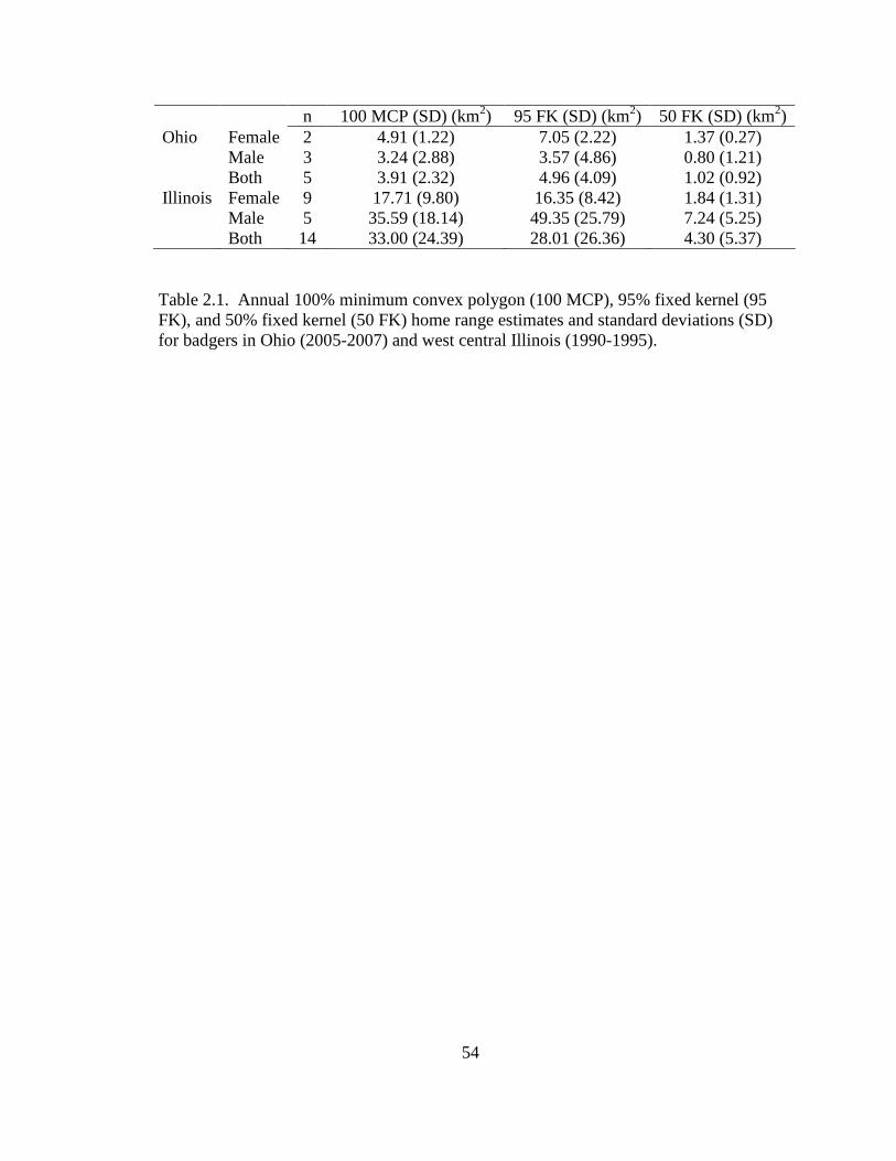
54

Table 2.1. Annual 100% minimum convex polygon (100 MCP), 95% fixed kernel (95 FK), and 50% fixed kernel (50 FK) home range estimates and standard deviations (SD) for badgers in Ohio (2005-2007) and west central Illinois (1990-1995).

n 100 MCP (SD) (km2) 95 FK (SD) (km2) 50 FK (SD) (km2) Ohio Female 2 4.91 (1.22) 7.05 (2.22) 1.37 (0.27) Male 3 3.24 (2.88) 3.57 (4.86) 0.80 (1.21) Both 5 3.91 (2.32) 4.96 (4.09) 1.02 (0.92) Illinois Female 9 17.71 (9.80) 16.35 (8.42) 1.84 (1.31) Male 5 35.59 (18.14) 49.35 (25.79) 7.24 (5.25) Both 14 33.00 (24.39) 28.01 (26.36) 4.30 (5.37)

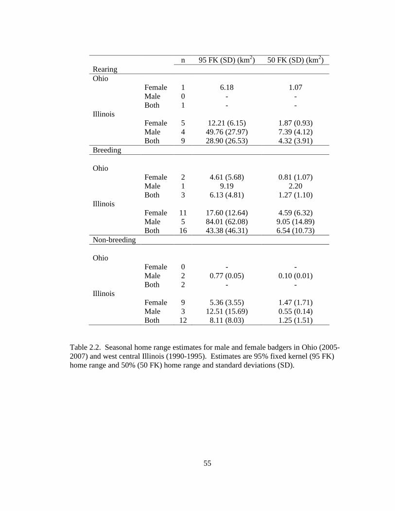
55

n 95 FK (SD) (km2) 50 FK (SD) (km2) Rearing Ohio Female 1 6.18 1.07 Male 0 - - Both 1 - - Illinois Female 5 12.21 (6.15) 1.87 (0.93) Male 4 49.76 (27.97) 7.39 (4.12) Both 9 28.90 (26.53) 4.32 (3.91) Breeding Ohio Female 2 4.61 (5.68) 0.81 (1.07) Male 1 9.19 2.20 Both 3 6.13 (4.81) 1.27 (1.10) Illinois Female 11 17.60 (12.64) 4.59 (6.32) Male 5 84.01 (62.08) 9.05 (14.89) Both 16 43.38 (46.31) 6.54 (10.73) Non-breeding Ohio Female 0 - - Male 2 0.77 (0.05) 0.10 (0.01) Both 2 - - Illinois Female 9 5.36 (3.55) 1.47 (1.71) Male 3 12.51 (15.69) 0.55 (0.14) Both 12 8.11 (8.03) 1.25 (1.51)

Table 2.2. Seasonal home range estimates for male and female badgers in Ohio (2005-2007) and west central Illinois (1990-1995). Estimates are 95% fixed kernel (95 FK) home range and 50% (50 FK) home range and standard deviations (SD).

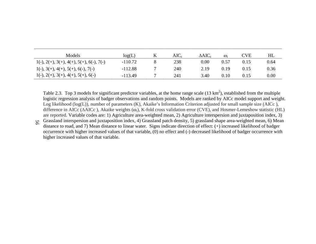
55

Table 2.3. Top 3 models for significant predictor variables, at the home range scale (13 km2), established from the multiple logistic regression analysis of badger observations and random points. Models are ranked by AICc model support and weight. Log likelihood (log(L)), number of parameters (K), Akaike’s Information Criterion adjusted for small sample size (AICc ), difference in AICc (∆AICc ), Akaike weights (ωi), K-fold cross validation error (CVE), and Hosmer-Lemeshow statistic (HL) are reported. Variable codes are: 1) Agriculture area-weighted mean, 2) Agriculture interspersion and juxtaposition index, 3) Grassland interspersion and juxtaposition index, 4) Grassland patch density, 5) grassland shape area-weighted mean, 6) Mean distance to road, and 7) Mean distance to linear water. Signs indicate direction of effect: (+) increased likelihood of badger occurrence with higher increased values of that variable, (0) no effect and (-) decreased likelihood of badger occurrence with higher increased values of that variable.

Models log(L) K AICc ∆AICc ωi CVE HL 1(-), 2(+), 3(+), 4(+), 5(+), 6(-), 7(-) -110.72 8 238 0.00 0.57 0.15 0.64

1(-), 3(+), 4(+), 5(+), 6(-), 7(-) -112.88 7 240 2.19 0.19 0.15 0.36 1(-), 2(+), 3(+), 4(+), 5(+), 6(-) -113.49 7 241 3.40 0.10 0.15 0.00

56

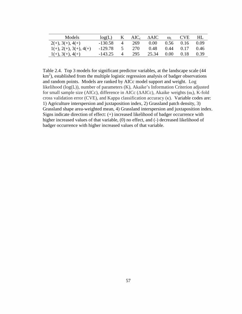
57

Models log(L) K AICc ∆AIC ωi CVE HL

2(+), 3(+), 4(+) -130.58 4 269 0.00 0.56 0.16 0.09 1(+), 2(+), 3(+), 4(+) -129.78 5 270 0.48 0.44 0.17 0.46 1(+), 3(+), 4(+) -143.25 4 295 25.34 0.00 0.18 0.39

Table 2.4. Top 3 models for significant predictor variables, at the landscape scale (44 km2), established from the multiple logistic regression analysis of badger observations and random points. Models are ranked by AICc model support and weight. Log likelihood (log(L)), number of parameters (K), Akaike’s Information Criterion adjusted for small sample size (AICc), difference in AICc (∆AICc), Akaike weights (ωi), K-fold cross validation error (CVE), and Kappa classification accuracy (κ). Variable codes are: 1) Agriculture interspersion and juxtaposition index, 2) Grassland patch density, 3) Grassland shape area-weighted mean, 4) Grassland interspersion and juxtaposition index. Signs indicate direction of effect: (+) increased likelihood of badger occurrence with higher increased values of that variable, (0) no effect, and (-) decreased likelihood of badger occurrence with higher increased values of that variable.

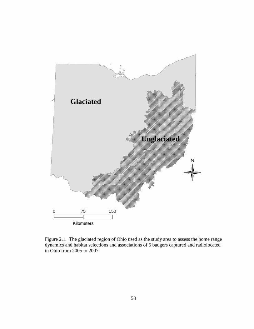
58

0 15075

Kilometers

Glaciated

Unglaciated

�

Figure 2.1. The glaciated region of Ohio used as the study area to assess the home range dynamics and habitat selections and associations of 5 badgers captured and radiolocated in Ohio from 2005 to 2007.

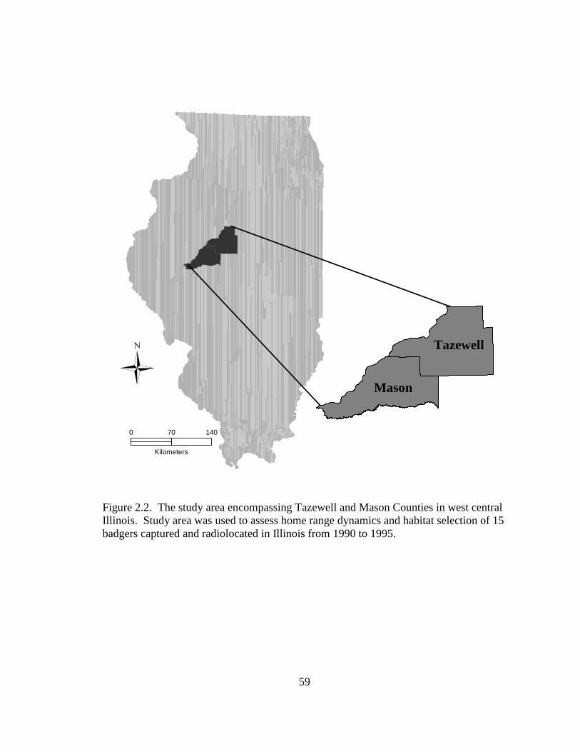
59

0 14070

Kilometers

Mason

Tazewell

�

Figure 2.2. The study area encompassing Tazewell and Mason Counties in west central Illinois. Study area was used to assess home range dynamics and habitat selection of 15 badgers captured and radiolocated in Illinois from 1990 to 1995.

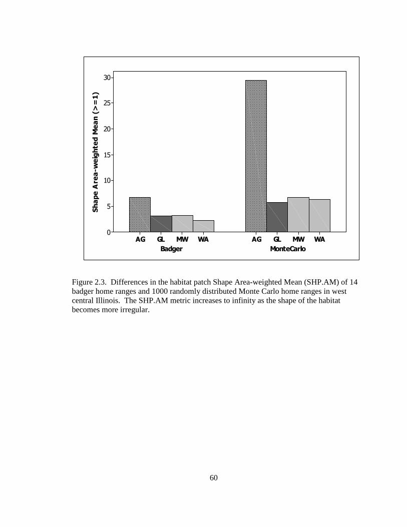
60

MonteCarloBadger

WAMWGLAGWAMWGLAG

30

25

20

15

10

5

0

Shape Area-w

eighted Mean (>=1)

Figure 2.3. Differences in the habitat patch Shape Area-weighted Mean (SHP.AM) of 14 badger home ranges and 1000 randomly distributed Monte Carlo home ranges in west central Illinois. The SHP.AM metric increases to infinity as the shape of the habitat becomes more irregular.

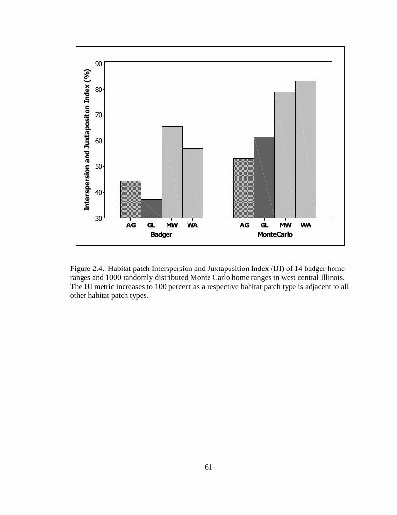
61

MonteCarloBadger

WAMWGLAGWAMWGLAG

90

80

70

60

50

40

30

Interspersion and Juxtapositon Index (%)

Figure 2.4. Habitat patch Interspersion and Juxtaposition Index (IJI) of 14 badger home ranges and 1000 randomly distributed Monte Carlo home ranges in west central Illinois. The IJI metric increases to 100 percent as a respective habitat patch type is adjacent to all other habitat patch types.

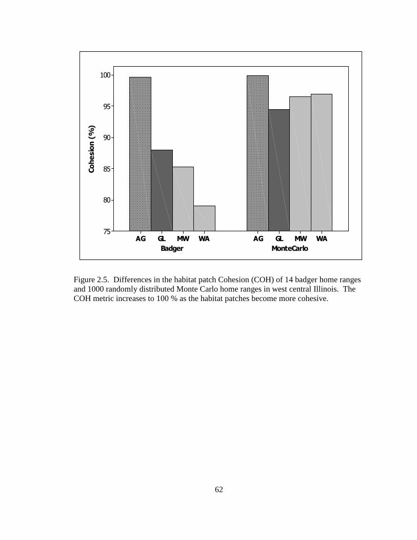
62

MonteCarloBadger

WAMWGLAGWAMWGLAG

100

95

90

85

80

75

Cohesion (%)

Figure 2.5. Differences in the habitat patch Cohesion (COH) of 14 badger home ranges and 1000 randomly distributed Monte Carlo home ranges in west central Illinois. The COH metric increases to 100 % as the habitat patches become more cohesive.

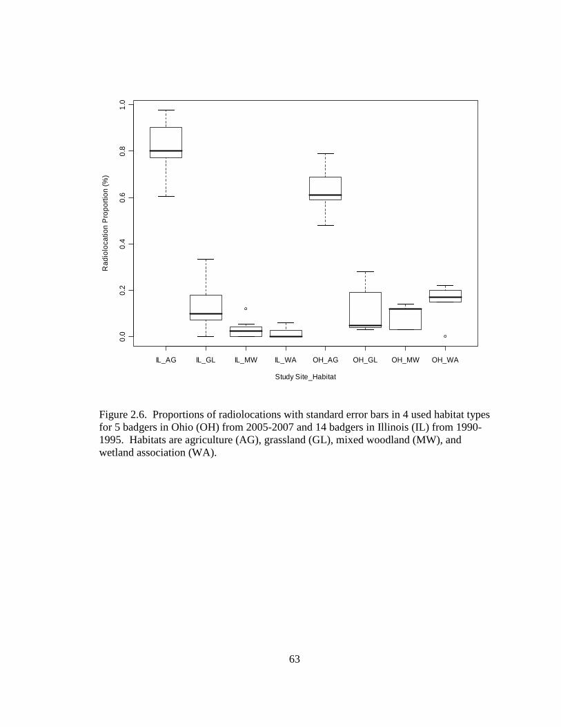
63

IL_AG IL_GL IL_MW IL_WA OH_AG OH_GL OH_MW OH_WA

0.0

0.2

0.4

0.6

0.8

1.0

Study Site_Habitat

Rad

iolo

catio

n P

ropo

rtion

(%)

Figure 2.6. Proportions of radiolocations with standard error bars in 4 used habitat types for 5 badgers in Ohio (OH) from 2005-2007 and 14 badgers in Illinois (IL) from 1990-1995. Habitats are agriculture (AG), grassland (GL), mixed woodland (MW), and wetland association (WA).

64

CHAPTER 3

BADGER (TAXIDEA TAXUS) HABITAT-RELATIVE ABUNDANCE I N OHIO

INTRODUCTION

Mammalian carnivores exhibit several characteristics (eg. territorial behavior,

large home range sizes, and low population densities) that may make these species

particularly vulnerable to habitat fragmentation. These species are commonly considered

sensitive indicators of environmental change (Zielinski et al. 2005) and therefore may

serve as umbrella species in which to assess habitat suitability for species not found in

this guild. Mammalian carnivore sensitivity to landscape fragmentation can result in

varied abundance and a non-uniform distribution across the landscape, particularly

related to prey availability and patch isolation (Crooks 2002). Within the mammalian

carnivore guild, mesocarnivores (e.g. medium-sized carnivores) vary in abundance based

on their habitat and dietary requirements. Habitat and dietary requirements, along with

territoriality, may greatly restrict the abundance of some mesocarnivore species, but not

others. Habitat and dietary generalist species such as the raccoon (Procyon lotor) are

more able to exploit a variety of habitat types and prey items compared to more specialist

species such as the American marten (Martes americana). Therefore, determining the

65

abundance of mesocarnivores across a given area may indicate wildlife responses to

habitat fragmentation and provide an understanding of the amount of suitable habitat and

prey in the area.

Mesocarnivore abundance over broad spatial scales has been investigated to better

understand the relationship between species, natural habitats, and human disturbances,

but is rarely estimated because of their low densities, use of large areas, and shy nature

(Kays et al. 2008). Mid-sized and small mammalian predators may be drivers of

ecosystem processes (e.g. regulating rodent populations) despite their relative rarity

across landscapes (Gompper et al. 2006). However, research efforts have been

overlooked or neglected in several mesocarnivore populations (Ray 2000, Hoodicoff

2003), and may additionally come as a result of their historic reputation as pests (Minta

and Marsh 1988). Many mesocarnivores found in the largely fragmented agricultural

matrix of the Midwestern United States remain relatively unstudied despite their role as

top predators in these landscapes. The American badger (Taxidea taxus) is one such

species that has remained relatively unstudied despite being a top predator and native to

the prairie habitat regions of the Midwest.

Badgers greatly vary in abundance across their North American range (Messick

and Hornocker 1981, Goodrich and Buskirk 1998, Warner and Ver Steeg 1995). Badger

density was reported as high as 5 badgers/km2 in a steppe/shrub landscape in Idaho

(Messick and Hornocker 1981), but was estimated as 0.14 badgers/km2 in a highly

fragmented agricultural landscape in west central Illinois (Warner and Ver Steeg 1995).

In states east of the Mississippi River no estimates of badger abundance are available,

with the exception of Illinois (Warner and Ver Steeg 1995). Moreover, estimates of

66

badger abundance and habitat requirements are lacking on the eastern edge of their

geographic distribution in Ohio. Species abundance is commonly higher near the center

of the distribution range, and population density declines toward most peripheral range

boundaries (Brown 1984). Therefore, badger density in Ohio is potentially lower than

estimates in other states toward the focal center of the badger range, which commonly

possess more favorable habitats (e.g. shrub-steppe) than that in Ohio. In addition,

badgers in Ohio are uncommon and listed statewide as a Species of Concern; however,

badger reports have proportionally increased in the past decade compared to past years

(Chapter 1). This recent increase in reports has led to an emphasis by the Ohio Division

of Wildlife (ODOW) to determine the habitat requirements and abundance of badgers in

Ohio. However, coupled with their uncommon status in Ohio, badgers are nocturnal and

cryptic, and therefore confound estimation of badger abundance.

Determining the abundance of a species occurring across a landscape, particularly

an uncommon and cryptic species such as the badger, presents a difficult task. To assess

badger abundance on a landscape scale, a relative measure must be utilized, as sample

plot counts or absolute counts would likely be futile for these cryptic carnivores. Several

authors have used known habitat requirements and home range estimates for respective

species to determine spatially explicit probabilities of that species occurring within a

large scale area (Clark et al. 1993, Dettmers and Bart 1999, Woolf et al. 2002, Twedt et

al. 2006, Preuss and Gehring 2007). Establishing spatially explicit probabilities for a

species across a landscape then allows for a relative measure of species abundance in the

study area. Further, this method has performed effectively using carnivore observation

and habitat use-availability data (e.g. Nielsen and Woolf 2002).

67

With known badger habitat requirements and home range estimates (Chapter 2)

this method provides a practical approach to predicting the habitat-relative abundance of

badgers in Ohio. Thus, I used badger observation and habitat use data, remotely sensed

land cover data, multivariate statistics, and a geographic information system (GIS) to

model the habitat-relative abundance and habitat suitability of badgers in Ohio.

METHODS

Study Area

The study encompassed all 88 counties in Ohio, from 38° 24‘N to 41° 59‘N and

80° 32° W to 84° 49° W. State-wide land cover was approximately 60% agriculture,

35% woodland/shrub, 3% urban, <1% open water, <1% wetland, and <1% barren (Ohio

Department of Development 2000). The glaciated central, western, and northwestern

regions of the state were characterized by a highly fragmented matrix of agriculture with

minimal topography. The remainder of the state was largely interspersed with forest and

agriculture, but was predominantly forested in the southeastern region. The geology and

associated landscape largely changed from glaciated alluvial soils to unglaciated soils of

sandstone and shale as defined by the Wisconsinan glacial line. Elevations gradually

decreased from north to south and range from 472 m to 139 m.

Badger Observations

From May 2005 to January 2008 I collected badger observations in the state-wide

study area with several methods. I solicited observations from wildlife professionals and

the public through an educational campaign which included presentations, observation

posters with tear-off report cards, fur harvester mail inquiry, and web-based discussion

forums. Records of badgers were also derived from the existing literature, historical

68

records from museum specimens, Ohio Division of Wildlife (ODOW) records, and the

Ohio Natural Heritage database. All badger observations were classified into 1 of 3

classifications based on the strength of evidence: confirmed (e.g. definitive evidence like

a road-kill or photograph), probable (observations from wildlife-related practitioners), or

unconfirmed (public report not positively confirmed).

Landscape Data

ArcGIS 9.1 (ESRI 2005) was used to perform all geographic information system

operations. I used the raster-based Ohio GAP land cover data (Center for Mapping, The

Ohio State University 2005) with a 30 m pixel resolution for spatial analysis. I

reclassified the Ohio GAP data from an original set of 40 land cover classes to 7 classes

(Appendix C), which included open water, agriculture, grassland, developed, mixed

woodland, barren/savanna, and wetland association. Reclassification was conducted in

order to reduce the number of potential parameters in the analysis. Finally, I used the

raster calculator in the Spatial Analyst in ArcGIS 9.1 to merge linear water and roadway

data to increase the accuracy of the land cover data in the study area.

Habitat Variable Selection

In order to select habitat variables that predicted badger occurrence I used a set of

badger observations and a multi-stage modeling approach. I first selected a subset of 134

confirmed and probable badger observations from 1990 to 2007 that were separated by at

least 1 week. These were chosen provided my assumptions that they were independent

observations and land use was not different from time of observation and that in the land

cover data used in analysis. These points were then geo-referenced and plotted on the

study area. Observation points were then circularly buffered using the mean 100% MCP

69

home range (x = 13.00 km2) size of female badgers in Illinois (Warner and Ver Steeg

1995) using the buffer tool in ArcGIS 9.1 (ESRI 2005). I acknowledge this home range

estimate is larger than those reported for Ohio (Chapter 2), but was used due to limited

home range estimates in Ohio.

An equal set of 134 points were then randomly plotted using Hawth’s Tools

(Beyer 2004) on the study area, but were not allowed to fall inside or within 2034 m (i.e

radius of observation buffer) of observation landscape buffers. This allowed the analysis

to take a detection or non-detection approach, where random point buffers were

presumed to be areas where badgers were not detected. I then used Hawth’s Tools to

individually clip badger observation and random point buffers from the reclassified land

cover.

I selected 10 landscape habitat and patch structure metrics that were similar to

reported badger habitat use from Illinois (Warner and Ver Steeg 1995) and Idaho

(Messick and Hornocker 1981). These metrics were then calculated for badger

observation and random point buffers using program FRAGSTATS (McGarigal and

Marks 1995). At the patch level I calculated the patch perimeter (PERIM) metric defined

as the perimeter of a patch in meters. At the class level I calculated the following

metrics: patch density (PD) defined as the number of patches per 100 ha; patch area-

weighted mean (AREAAM) defined as the total area (ha) of patches multiplied by the

proportional abundance of the patch; shape area-weighted mean (SHPAM) gives a

relative measure of patch shape multiplied by the proportional abundance of the patch,

which increases without limit from 1 as a patch deviates from a square block;

interspersion and juxtaposition index (IJI) defined as the percentage of a habitat patch

70

being adjacent to 1 other habitat patch type (0 percent) or all other habitat patch types

(100 percent); patch cohesion (COH) defined as the proportion (0-100) of habitat patch

connectedness where a value of 100 would be complete focal habitat patch

connectedness; related circumscribing circle (CIRCLE) gives a relative measure (0-1) of

patch elongation, where 1 equals a highly elongated linear patch; and Euclidean nearest

neighbor distance area-weighted mean (ENNAM) defined as the distance in meters to

nearest neighboring patch of the same habitat type. At the landscape level I calculated

Simpson’s Diversity Index (SIDI) which gives a relative measure (0-1) of patch richness

in an area where SIDI of 1 equals maximal patch richness; and Simpson’s Evenness

Index (SIEI) which gives a relative measure (0-1) of patch distribution across an area

where SIEI of 1 equals proportional distribution of patch types across an area.

In order to reduce the number of potential habitat variables I first conducted a

Spearman Rank correlation analysis to account for multicollinearity between variables. If

a pair of variables was found to be highly correlated (R2 ≥0.6) I removed 1 of the

variables believed to be less biologically important to badgers. I then univariately

conducted binary logistic regression to determine if badger observation buffer data were

different than random buffer data. I retained variables that were significant (α = 0.10)

and were supported by the Hosmer-Lemeshow goodness of fit statistic. Because of

multiple potential predictor variables an information theoretic modeling approach using

multimodel inference corrected for small sample size (AICc) (Burnham and Anderson

2002) was used to determine the best model of variable combinations (Table 3.1). I

additionally evaluated the fit of models using the Kappa statistic to test for correct

classification of model and further used K-fold cross validation to assess the error in

71

model fit, using 5 folds. All statistical analysis was conducted using R for Windows

version 2.4.1 (R Development Core Team 2006).

Abundance Estimation

I produced a continuous coverage of 3,861 non-overlapping hexagons of 13.0 km2

(i.e., x size of female MCP home ranges; Warner and Ver Steeg 1995) that covered the

entire state-wide study area, but did not overlap the state boundaries. This hexagon

coverage was then overlaid on the reclassified land cover and significant variables (Table

3.1) were calculated for each hexagon using the Patch Analyst Grid 3.0 extension to

ArcView GIS 3.2. Further analysis required data normality and therefore I used the

natural log transformation for agriculture area-weighted mean and grassland patch

density. All other variables followed approximate normal distributions.

I then developed a model of habitat similarity in the state-wide study area based

on the significant habitat variables from badger observations (Table 3.1). I calculated the

mean habitat vector as the mean values of significant variables in hexagons which

contained the 134 badger observations (Figure 3.1). The Penrose distance (PD) statistic

was then used to measure habitat similarity between the mean vector from badger

observation buffers and habitat characteristics within each hexagon of the study area. I

calculated the Penrose distance as,

pVkukjukiPijp

k

/)[(2

1

−=∑=

where population i represented badger observation buffers, population j represented study

area hexagons, p was the number of habitat variables evaluated, u was the variable value,

k was each observation, and V was variance (Manly 2005). Hexagons with values closer

72

to 0 were most similar to areas of associated badger habitat based on collected

observations, whereas increasing values indicated increased dissimilarity to associated

habitat. I used a spreadsheet for all calculations and appended the final Penrose distance

output to the hexagon grid in ArcMap GIS 9.1 to create a map of Penrose distance

throughout the state-wide study area.

Model Classification

A set of core home range areas and capture locations (n = 9) were used to classify

hexagons for likelihood of badger occurrence across the state. I plotted 50% MCP core

home ranges or capture sites of badgers in Ohio (Chapter 2) on the Penrose hexagon

coverage. I then selected each hexagon that contained a badger core home range or

capture site and recorded the PD for those hexagons. The mean PD for badger core home

ranges was then calculated and was used as the cut point for the likelihood of having at

least 1 badger in a respective hexagon. I used the highest Penrose value of all badger

core areas or capture sites as the middle cut point to determine an intermediate likelihood

classification. Hexagons with Penrose values above the intermediate classification were

those with unlikely badger occurrence.

RESULTS

Comparisons of badger observation buffers and the study area showed distinct

differences in the mean area of agriculture patches, density and shape of grassland

patches, and overall evenness and diversity of habitat types. Badger observation buffers

contained one-fourth the mean patch size of agricultural habitat, twice the grassland patch

density, had more interspersed block-like grassland patches compared to the study area.

Also, badger buffer areas contained a more even diversity of habitat types than the study

73

area. Although significant, the number of different habitat types was not markedly

different between badger buffers and the study area. Grassland area-weighted shape and

agriculture interspersion and juxtaposition index were most correlated to PD (Table 3.1).

The mean PD for badger observation buffers was 214.60, SE = 48.00, range =

0.00-4953.40, and for the study area was 280.80, SE = 31.30, range = 0.00-79508.50.

Mean Penrose distance for badger core home ranges used to classify the likelihood of

badger occurrence was 7.35, SE = 2.93, range = 0.00-23.87. Across the study area, 83%

of hexagons were less than or equal to the mean PD (214.60) of badger observations,

suggesting the majority of the state possessed likely badger occurrence based on habitat

metrics evaluated. However, a priori I assumed that badgers were uncommon in the state

and habitat and patch structure metrics of radioharnessed badger core home ranges

reduced the likelihood of badger occurrence across several regions of the state. Mean PD

of badger core home ranges determined 51% hexagons were ≤7.4 (i.e. those with likely

badger occurrence), 13% hexagons were >7.4 but ≤23.9 (i.e. those with intermediate

badger occurrence), and 36% hexagons were >23.9 (i.e. those with unlikely badger

occurrence). Least average PD (i.e. those most similar to badger core home ranges)

mainly occurred in the northwest, southwest, and north central regions of the state

(Figure 3.2). Penrose distance was greatest in the southeast region of the state-wide study

area and in the major metropolitan areas. Predicted relative abundance was relatively

uniform in the northwest and north central regions of the state, with a uniform pocket of

likely occurrence in the south central region (Figure 3.3). The remainder of the state was

interspersed with likely to unlikely badger occurrence.

74

DISCUSSION

Overall agriculture and grassland habitats were associated with badger occurrence

across the study area. Grassland shape area-weighted mean was most important in

determining PD across the study area and indicated badger observation buffers contained

more block shaped grassland patches than did the study area. In addition, agriculture

area-weighted mean, grassland patch density, and Simpson’s evenness index were

significantly different on their respective scales between badger observations buffers and

the study area. These differences suggest that badger density is likely highest where

interspersed small even area blocks of agriculture and grassland occur. Although their

means were not largely different from study area, the agriculture and grassland

interspersion and juxtaposition indexes were significant in analyses. These also help to

support the importance of these interspersed habitats as they possessed larger values for

badger observation buffers than the study area.

The model was intended to provide an estimate of badger habitat-relative

abundance in Ohio. Badgers in Ohio are presumed to be uncommon and highly cryptic,

therefore hindering absolute abundance estimation. To circumvent these limitations, use

of the PD statistic to measure the spatially explicit similarity between badger habitat

associations and the state-wide study area was considered an appropriate method to

model badger relative abundance. Similarly, this method has been used to model the

habitat-relative abundance of bobcats (Lynx rufus) in Illinois (Nielsen and Woolf 2002)

and Michigan (Preuss and Gehring 2007). However, opposite of those authors, I used

observational data to first obtain habitat variables that predicted badger occurrence and

then classified the model with known badger core home range PD values. Although

75

habitat variables important to badgers at the home range scale were used to develop the

habitat-relative abundance, this estimate should be considered cautiously. Badgers use a

range of habitats and patch structures in the study area at multiple spatial scales (Chapter

2) and therefore badger density may varying depending on the availability of habitat

across this highly fragmented study area. In addition, due to limited sample size in Ohio,

abundance estimates were based on the mean female badger home range size reported in

Illinois (Warner and Ver Steeg 1995). As a result, the scale (e.g. mean Illinois female

home range) at which the model is represented may be different from that at which

badgers in Ohio use the landscape, however home ranges were thought to be similar to

those in Illinois due to similar study site characteristics in Ohio. Finally, habitat variables

thought to be important to badgers were derived from observations and therefore may not

truly represent actual habitat use by badgers in Ohio. Despite this inherent limitation in

habitat use data, I used a recent (i.e. 1990 to 2007) set of observations that were screened

for valid badger characteristics and known badger core home ranges in Ohio to establish

and classify density in the study area. Thus, I believe this model is a suitable

representation of badger habitat-relative abundance in Ohio.

The model is largely representative and closely follows the state-wide distribution

of badgers established from collected observations (Chapter 1). The distribution (Figure

1.3) fundamentally supports the model as hexagons with higher probabilities of badger

density (i.e. 0.75-1.00) are generally clustered in counties with higher counts of badger

observations. These counties are mainly found in the northwest, southwest, and north

central regions of the state, which are relatively uniform regions of high predicted badger

abundance. In addition, the abundance model (Figure 3.3) shows a general pattern of

76

discerning higher badger density above the glacial line in Ohio; which is also shown on

the state-wide distribution map. Above this line exists a highly fragmented matrix of

agriculture with relatively minimal topography and alluvial glacial till soils, whereas

below the glacial line topography consists of largely forested hills with stone or shale

soils. Badger habitat and therefore abundance are likely limited in most areas found

below the glacial line.

The spatially explicit model has applicability to future population survey efforts

in Ohio. Although the model was developed to investigate the habitat-relative abundance

of badgers, it only provides explicit areas of where badger occurrence is more likely than

compared to others. However, areas (i.e. hexagons) where badger occurrence was likely

possess habitats that badgers are associated with and known to use in the state. Therefore

this model can provide a useful tool to identify areas where badger habitat is lacking and

where conservation efforts should be focused.

77

LITERATURE CITED Beyer, H. L. 2004. Hawth's Analysis Tools for ArcGIS. <http://www.spatialecology.com/htools>. Accessed 15 Sep 2006. Brown, J.H. 1984. On the relationship between abundance and distribution of species. American Naturalist 124: 255-279. Burnham, K.P., and D.R. Anderson. 2002. Model selection and multimodel inference. Second edition. Springer, New York, USA. Clark, J.D., J.E. Dunn, and K.G. Smith. 1993. A multivariate model of female black bear habitat use for a GIS. Journal of Wildlife Management 57: 519-526. Crooks, K.R. 2002. Relative sensitivities of mammalian carnivores to habitat fragmentation. Conservation Biology 16: 488-502. Dettmers, R., and J. Bart. 1999. A GIS modeling method applied to predicting forest songbird habitat. Ecological Applications 9: 152-163. Environmental Systems Research Institute, Inc. 2005. ArcGIS 9.1. Redlands, CA. Gompper, M.E., R.W. Kays, J.C. Ray, S.D. Lapoint, D.A. Bogan, and J.R. Cryan. 2006. A comparison of noninvasive techniques to survey carnivore communities in northeastern North America. Wildlife Society Bulletin 34: 1142-1151. Goodrich, J.M., and S.W. Buskirk. 1998. Spacing and ecology of North American badgers (Taxidea taxus) in a prairie-dog (Cynomys leucurus) complex. Journal of Mammalogy 79: 171-179. Hoodicoff, C.S. 2003. Ecology of the badger (Taxidea taxus jeffersoni) in the Thompson region of British Columbia: implications for conservation. M.S. Thesis. University of Victoria, Victoria. 111pp. Kays, R.W., M.E. Gompper, and J.C. Ray. 2008. Landscape ecology of eastern coyotes based on large-scale estimates of abundance. Ecological Applications 18: 1014- 1027. Manly, B. F. J. 2005. Multivariate statistical methods: a primer. Third edition. Chapman and Hall/CRC Press, Boca Raton, Florida, USA.

78

McGarigal, K., and B.J. Marks. 1995. FRAGSTATS: spatial pattern analysis program for quantifying landscape structure. Version 3.3. United States Forest Service General Technical Report PNW-GTR-351, Portland, Oregon, USA. Messick, J.P., and M.G. Hornocker. 1981. Ecology of the badger in southwestern Idaho. Wildlife Monographs 76. 56pp. Minta, S.C., and R.E. Marsh. 1988. Badgers (Taxidea taxus) as occasional pests in agriculture. Proceedings of the Vertebrate Pest Conference 13: 199-208. Nielsen, C. K., and A. Woolf. 2002. Habitat-relative abundance relationship for bobcats in southern Illinois. Wildlife Society Bulletin 30:222–230. Ohio Department of Development, Office of Strategic Research. 2000. Ohio County Profiles. Appendix B: Sources. Land Cover. Preuss, T.S., and T.M. Gehring. 2007. Landscape analysis of bobcat habitat in the northern lower peninsula of Michigan. Journal of Wildlife Management 71: 2699-2706. Ray, J.C. 2000. Mesocarnivores of northeastern North America: status and conservation issues. Wildlife Conservation Society Working Paper 15: 1–82. R Development Core Team. 2006. R: a language and environment for statistical computing. R Foundation for Statistical Computing, Vienna, Austria. The Ohio State University. Center for Mapping. 2005. Ohio GAP program land cover data. Twedt, D.J., W.B. Uihlein, and E.A. Blaine. 2006. A spatially explicit decision support model for restoration of forest bird habitat. Conservation Biology 20: 100-110. Warner, R.E. and B. Ver Steeg. 1995. Illinois Badger Studies. Division of Wildlife Resources. Department of Natural Resources and Environmental Sciences. Springfield, Illinois. 161pp. Woolf, A., C.K. Nielsen, T. Weber, and T.J. Gibbs-Kieninger. 2002. Statewide modeling of bobcat, Lynx rufus, habitat in Illinois, USA. Biological Conservation 104: 191-198. Zielinski, W.J., R.L Truex, F.V. Schlexer, L.A. Campbell, and C. Carroll. 2005. Historical and contemporary distributions of carnivores in forests of the Sierra Nevada, California, USA. Journal of Biogeography 32: 1385-1407.

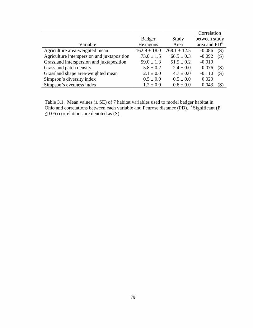
79

Table 3.1. Mean values (± SE) of 7 habitat variables used to model badger habitat in Ohio and correlations between each variable and Penrose distance (PD). a Significant (P ≤0.05) correlations are denoted as (S).

Variable Badger

Hexagons Study Area

Correlation between study area and PDa

Agriculture area-weighted mean 162.9 ± 18.0 768.1 ± 12.5 -0.086 (S) Agriculture interspersion and juxtaposition 73.0 ± 1.5 68.5 ± 0.3 -0.092 (S) Grassland interspersion and juxtaposition 59.0 ± 1.3 51.5 ± 0.2 -0.010 Grassland patch density 5.8 ± 0.2 2.4 ± 0.0 -0.076 (S) Grassland shape area-weighted mean 2.1 ± 0.0 4.7 ± 0.0 -0.110 (S) Simpson’s diversity index 0.5 ± 0.0 0.5 ± 0.0 0.020 Simpson’s evenness index 1.2 ± 0.0 0.6 ± 0.0 0.043 (S)

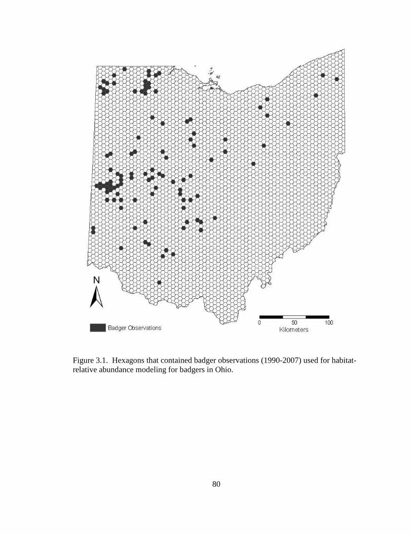
80

Figure 3.1. Hexagons that contained badger observations (1990-2007) used for habitat-relative abundance modeling for badgers in Ohio.

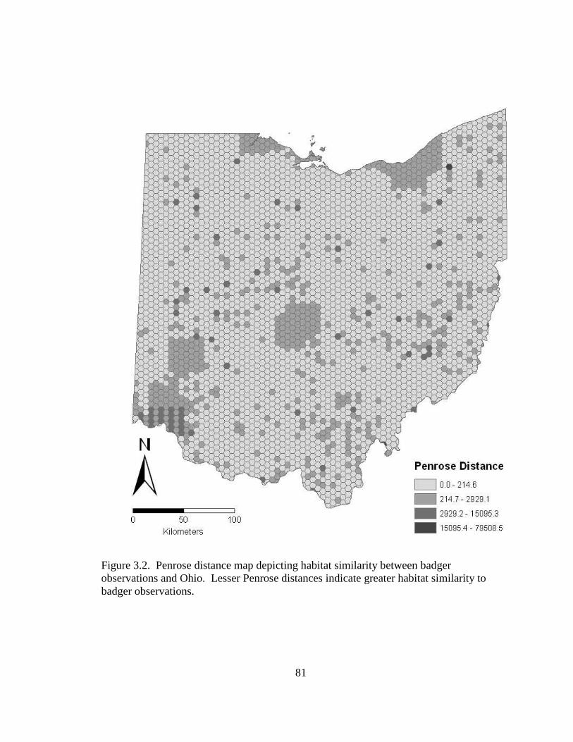
81

Figure 3.2. Penrose distance map depicting habitat similarity between badger observations and Ohio. Lesser Penrose distances indicate greater habitat similarity to badger observations.

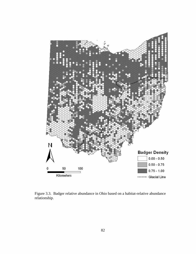
82

Figure 3.3. Badger relative abundance in Ohio based on a habitat-relative abundance relationship.

83

CHAPTER 4

POPULATION DEMOGRAPHY AND DIET OF BADGERS (TAXIDEA TAXUS) IN OHIO

INTRODUCTION

Carnivores are generally considered members of the same guild but are

heterogeneous in their sensitivities to landscape and local fragmentation (Crooks 2002).

This heterogeneity can lead to varied responses in carnivore abundance, persistence, and

interactions among species (Ryall and Fahrig 2006). Landscape fragmentation can lead

to changes in the physical environment as well as biogeographical changes (Saunders et

al. 1991). These changes can affect wildlife in many ways but can result in species edge

effects (Heske 1995, Dijak and Thompson 2000) and potentially the isolation and local

extinction of carnivores (Crooks 2002). The effects of landscape fragmentation can in

turn have large influences on the vital rates of species because habitat patches may, for

example, become more isolated or disconnected and consequently hindering movement

of individuals. The survival and reproduction of carnivores may be affected by landscape

fragmentation because individuals are forced to move greater distances to meet their

biological requirements. Due to their environmental sensitivity and trophic position,

84

some carnivores may serve as indicators of ecosystem integrity (Noss et al. 1996)

Therefore estimates of carnivore population demography may be important for

understanding how these species respond to human-dominated landscapes and

fragmentation.

Estimates of abundance, survival, reproduction, and sex ratios are intrinsic to both

population models and management actions dealing with factors such as harvest,

endangered species, and control of exotics (Mills 2007). In addition, population and

morphometeric information are necessary to understand species function and interactions

at the community and ecosystem levels (Rosalino et al. 2005). This information can then

be used to assess the population status and trend of a species, potentially over a long time

period. If the population indicates an increasing or declining trend then rates of

fecundity, survival, immigration, and emigration that influence the persistence of a

carnivore population must be known (Gese 2001). Vital rates of many carnivore species

have been included in demographic population models to assess the population status and

trend (Carroll et al. 2003). However, population status is basically unknown for many

mesocarnivore species because of their secretive habits, limited research support, and low

economic value (Ray 2000). As such, the population status of the American badger

(Taxidea taxus) is relatively unknown across its geographic range.

Estimation of demographic parameters and diet composition is essential in the

management of a top predator like the badger. Harvest rates of many furbearers are

frequently modeled with vital rate estimates to project the future population trend of a

species (Mills 2007). However, the population status of the badger largely varies

geographically with density and landscape habitat suitability, and caution should be taken

85

with extrapolation of vital rate parameters across different landscapes. In addition,

badgers are known to exhibit disparate prey choice patterns and rely upon a prey base

that is both diverse and spatio-temporally variable (Azevedo et al. 2006). Thus,

identifying the diet composition of badgers could provide inferences to food availability

in the environment and present insights into their key foraging habitats.

Estimates of vital rates and diet information for badgers have primarily come

from the western and plain regions of the United States where population densities are

relatively high and suitable habitat is abundant. Estimates of badger vital rates are not

totally comparable because they have been estimated in different ways, but are useful for

a basic understanding of badger biology. In southwestern Idaho, the proportion of

breeding females was shown to range from 0.33 to 0.58 and average litter size was 1.7

(Messick and Hornocker 1981). In Utah and Idaho a mean of 2.2 corpora lutea were

counted in 27 badgers (Lindzey 1971) and similarly, Todd (1980) estimated average litter

size to be 2.2 from counts of corpora lutea, placental scars, and field counts of litters in

southern Idaho. Wright (1966) suggested that most adult female badgers breed, but few

breed during their first summer (i.e. at 4-5 months old). This was also supported by

Messick et al. (1981) who found the proportion of parous or pregnant females in all age

classes in southwestern and south central Idaho was 52% (N = 167) and 72% (N = 62)

respectively. Messick et al. (1981) also reported that in Idaho the proportion of females

that bred during their first summer and gave birth at 12 months old ranged from 40% (N

= 50) to 52% (N = 27).

Several studies have also documented badger dietary composition in several

regions of the species’ range. Sciuridae species were the most common prey item in

86

Iowa (Errington 1937, Snead and Hendrickson 1942) and South Dakota (Jense 1968). In

east central Minnesota, pocket gophers (Geomys bursarius) were the primary prey

species; however, 14 other mammal species were found in diet contents (Lampe 1982).

Microtine and cricetine rodents had the highest frequency of occurrence, followed by

lagomorphs, in Utah and Idaho (Lindzey 1971). Diets of badgers in west central

Minnesota and southeastern North Dakota primarily consisted of small mammals from

Muridae or Geomyidae, but also contained remains of insects, birds, reptiles, amphibians,

and mollusks (Sovada et al. 1999). This breadth in diet was also observed in badger

carcasses collected from 2000 to 2001 in Saskatchewan, Canada (Azevedo et al. 2006).

Badger diets typically vary seasonally in response to prey availability. Diet

contents of badgers collected during summer months have shown a greater diversity of

small mammal species (Lampe 1976) and alternative prey (e.g. reptiles and birds)

(Sovada et al. 1999) compared to other seasons. Messick and Hornocker (1981) observed

seasonal and yearly changes in badger diets that corresponded to shifts in prey

availability; where badgers consequently shifted more to lagomorphs and other rodents in

response to declines in Townsend ground squirrels (Spermophilus townsendii). Also,

sub-adult badgers have been observed to eat more arthropods and birds and fewer

mammals than adults. This sub-optimal diet may have resulted from undeveloped

predatory skills and dispersal (Messick 1999).

Past studies have provided various parameter estimates of badger demography

and dietary information, but were conducted in landscapes dissimilar to that in Ohio.

These data are useful for badger population management in those regions but are limited

for extrapolation to areas east of the Mississippi River where virtually no information

87

exists on badger demography and diet. However, Warner and Ver Steeg (1995) shed

some light on badger demography and diet in a highly fragmented agricultural landscape

in west central Illinois. Illinois badgers exist at low density, estimated at 0.14

badgers/km2 and fecundity was estimated as 0.32 young/female from a mean litter size of

1.67 and a 0.27 sub-adult survival rate. Also, badgers consumed mainly small

mammalian prey, but also contained 21% reptiles or amphibians. Estimates of adult

fecundity and survival of young badgers in west central Illinois are lower than those

reported in western states with greater suitable habitat. These estimates from Illinois

provide some inference to badger demography east of Mississippi River in a fragmented

agricultural landscape. However, badger population demography remains highly

equivocal on the eastern fridge of their geographic range in Ohio.

Badgers are uncommon and likely exist at low density in Ohio, making

population demography and diet composition difficult to determine. The species is native

to the historical prairie regions of Ohio and was a harvestable furbearer in Ohio until

1990, when it was protected statewide as a Species of Concern. This protection was

afforded mainly as a result of their uncommon status and unknown ecology in the state.

In the past 10 to 20 years, reports of badger observations have been increasing (Chapter

1), yet it is unknown if these increased reports are the result of an increase in population

size, range expansion, increased human development, or a combination of several factors.

Badgers have presumably expanded their range eastward in the Midwestern United States

with large scale deforestation practices, chiefly for agricultural use (Lyon 1932, Moseley

1934, Leedy 1947, Nugent and Choate 1970, Gremillion-Smith 1985, Warner and Ver

Steeg 1995, Berkley and Johnson 1998). Land use practices over the past 2 centuries

88

have now transformed Ohio from its historical matrix of forest and native prairie pockets

into primarily a highly fragmented agriculture landscape. Badgers are fossorial

mesocarnivores which are commonly associated with prairie, open grasslands, and other

treeless habitats (Messick 1999) and therefore deforestation has likely provided these

mustelids with greater suitable habitat (Chapter 1). While the eastern range extension of

badgers has been documented, there remains a paucity of research on the population

status and demography of badgers in this highly fragmented agricultural region.

Demography and diet data are essential to further understanding badger ecology

and establishing management initiatives for the species in Ohio. Due to the species

uncommon status and low density population, female survival and reproduction are

especially important to estimate given that female vital rates can dramatically alter

population viability. In addition, badger survival and fecundity vary with human activity

and badger density (Messick and Hornocker 1981). Thus projecting the population with

differential parameters would likely prove useful to evaluate different population

scenarios, which could incorporate simulated harvest. With these considerations in mind

a population projection matrix provides a useful tool to incorporate female vital rates and

evaluate several population scenarios. To provide state wildlife practitioners with

population information for future management of the badger in Ohio, my objectives were

to determine: 1) diet composition, 2) sex ratio, 3) age structure, 4) body and skull

morphometrics, 5) reproductive status, and 6) population projections using a Leslie

population matrix.

89

METHODS

Carcass Collection and Necropsy

Badger carcasses were collected state-wide from May 2005 to June 2008. Basic

necropsies and evaluations were conducted to obtain gastrointestinal contents, sex, age

structure, morphometrics, and reproductive status. The collection date, location, age, sex,

cause of mortality, reproductive status, and baculum length and weight of each carcass

was recorded (Appendix K). To determine mortality by season I defined 3 biological

seasons that were based upon the life cycle of female badgers. I defined 3 biological

seasons that were based upon the life cycle of female badgers (Warner and Ver Steeg

1995). I defined the rearing (spring) season from March 1 to June 30 and represents a

period when movements by breeding females are commonly restricted by parturition and

rearing young (Messick and Hornock 1981). The breeding (summer) season was defined

from July 1 to October 30 and the non-breeding (winter) season from November 1 to

February 28, during which badgers largely restrict their activity and home range sizes

shrink considerably (Lindzey 1978, Messick 1999).

Diet Composition

Badger gastrointestinal contents were extracted and run through a 1.0 mm and 0.5

mm sieve to separate contents. Contents were dried in paper bags for ≥5 days and

separated into broad categories based on type of remains (e.g. hair and bone). Hair was

fixed to a glass slide and identified under a compound microscope to a species or genus

level using known species hair samples and a hair identification guide. Bone remains

were identified to the species specific or genus level using a bone identification guide.

Other contents could be identified by basic evaluation (e.g. plant material). I assumed

90

that badger hair found in remains was a result of grooming and was not quantified.

Presence of prey items were recorded individually for each badger and then summed over

all badgers. Total occurrence for each prey item was then divided by the total number of

prey items found overall and by season to derive a percentage of total occurrence in diet.

Sex

Badger sex was determined through external evaluation for the presence of testes

and penal opening (males) or presence of teats and vaginal opening (females). However,

in some cases carcasses were depredated or characteristics to identify sex were missing,

and sex was then recorded as unknown.

Age Structure

Badger age was determined through cementum analysis of collected teeth (Crowe

and Strickland 1975). If available, the lower right canine was extracted, but another

canine or second premolar was taken if canine not was present or broken. Teeth were

then sent to Matson’s Laboratory LLC (Milltown, MT) for cementum aging. Age classes

were defined as YY ≤1 year of age, sub-adults 1-2 years of age, and adults ≥2 years of

age.

Morphometrics

Basic morphometric data were collected on the body length and weight, right hind

foot, right ear, tail, and skull. Body length was measured from the tip of the nose to the

last vertebrae of the tail. Body weight was taken on animals that contained all organs and

tissues, pelted animals were corrected by multiplying skinned body weight by 1.2 to give

an approximate estimate of original weight with pelt. The right hind foot was measured

from the tip of the front pads to the rear tip of the hind pad. The right ear was measured

91

from the tip of the ear to the bottom of the ear canal. The tail was measured from the first

tail vertebrae to the last tail vertebrae. Skulls were cleaned and boiled in water and

acetone for approximately 60 min to remove flesh and oil and then dried for ≥10 days.

Skull measurements followed Long (1972) and included the greatest length of skull,

zygomatic breadth, postorbital breadth, palatal length, alveolar length maxillary

toothrow, carnassial length, and cranial depth.

Male YY morphometrics were compared to those of female YY and male badgers

≥1 year of age were compared to those of females ≥1 year of age. Also, male YY were

compared to males ≥1 year of age and female YY were compared to females ≥1 year of

age. For comparisons, a 2-sample t-test with equal variances was used. All statistical

analysis was done in R for Windows version 2.4.1 (R Development Core Team 2006).

Reproductive Status

Female badger carcasses were externally evaluated for signs of potential or

realized fecundity. Potential fecundity was recorded as presence of lactation or

blastocysts. Realized fecundity was recorded as presence of placental scars or embryos.

Bacula in males were cleaned and boiled in water and acetone for approximately 30 min

to remove oil and were then dried for ≥10 days. Bacula were then measured after the

drying period from the top tip to the bottom tip and weighed using an electronic scale.

Female uterine tracts were extracted and evaluated for presence of blatocysts or placental

scars. I looked for blastocysts first by injecting and thoroughly flushing each uterine

horn 3 times with saline water into a clear glass petri dish. I then linearly cut each uterine

horn and looked for presence of placental scars under a dissecting microscope and naked

eye. The number of blastocyts and embryos were recorded for potential fecundity and

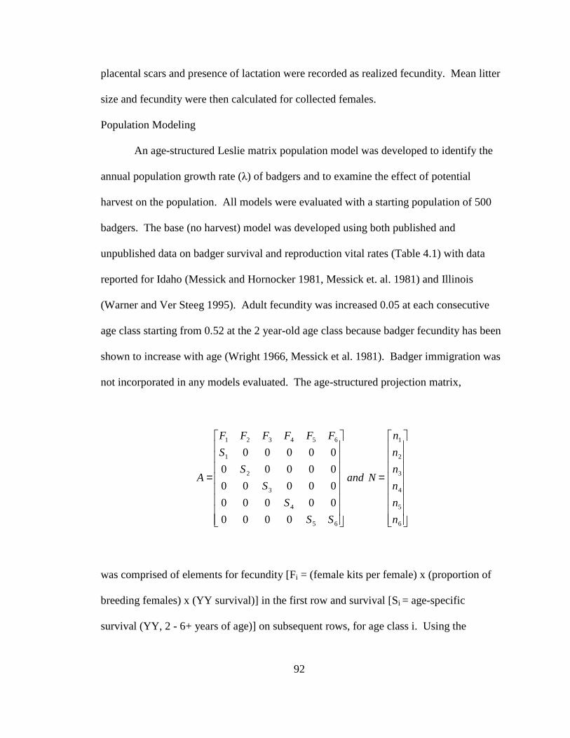
92

placental scars and presence of lactation were recorded as realized fecundity. Mean litter

size and fecundity were then calculated for collected females.

Population Modeling

An age-structured Leslie matrix population model was developed to identify the

annual population growth rate (λ) of badgers and to examine the effect of potential

harvest on the population. All models were evaluated with a starting population of 500

badgers. The base (no harvest) model was developed using both published and

unpublished data on badger survival and reproduction vital rates (Table 4.1) with data

reported for Idaho (Messick and Hornocker 1981, Messick et. al. 1981) and Illinois

(Warner and Ver Steeg 1995). Adult fecundity was increased 0.05 at each consecutive

age class starting from 0.52 at the 2 year-old age class because badger fecundity has been

shown to increase with age (Wright 1966, Messick et al. 1981). Badger immigration was

not incorporated in any models evaluated. The age-structured projection matrix,

=

=

6

5

4

3

2

1

65

4

3

2

1

654321

0000

00000

00000

00000

00000

n

n

n

n

n

n

Nand

SS

S

S

S

S

FFFFFF

A

was comprised of elements for fecundity [Fi = (female kits per female) x (proportion of

breeding females) x (YY survival)] in the first row and survival [Si = age-specific

survival (YY, 2 - 6+ years of age)] on subsequent rows, for age class i. Using the

93

projection matrix, variations in population size and age structure (N) can be calculated

between times t and t + 1 from the equation:

tt ANN =+1

The base model was constructed using only the female portion of the population

(assuming a 1:1 sex ratio) using a density independent model with a yearly time step.

Stable age distribution (WA) for the population was calculated from the right eigenvector

associated with the dominant eigenvalue (λ). Reproductive value (VA) for individuals in

each age group is the left eigenvector and gives the expected relative contribution of a

female currently in a given age group to future population growth.

To assess the effect of a simulated population harvest an estimated harvest rate of

0.045 was applied to each age class using the base model. This estimate was used by

Warner and Ver Steeg (1995) to assess a simulated harvest on a low density badger

population in west central Illinois. I also created 4 population models that described 4

different scenarios based on different rates of YY breeding and survival. These models

were created because YY breeding and survival has been shown to vary locally and

regionally between geographic study areas across the United States (Messick and

Hornocker 1981, Messick et al. 1981, Warner and Ver Steeg 1995), which may largely

affect future population trends. In addition, 4 population models were created to describe

4 different scenarios based on differential female YY breeding and survival and a

fecundity increase of 0.05 at each consecutive age for adults. Fecundity was increased

0.05 per adult year to approximate fecundity estimates in western states (Messick and

94

Hornocker 1981).

RESULTS

I collected 46 badger carcasses during May 2005 to June 2008. Carcasses

consisted of 18 males, 24 females, and 4 with unknown sex. The male to female sex ratio

did not differ from 1:1 (t = -0.78, df = 41, P = 0.442). Known age data were available for

38 badgers and the overall mean age was 1.63, SD = 1.57, range 0 – 6 years (Figure 4.1),

with females 1.47, SD = 1.71, range = 0 – 6 years, n = 19, and males 1.88, SD = 1.45,

range = 0 – 5 years, n = 17 (Table 4.2). The oldest badger recovered was a 6 year-old

female (B35). Age categories consisted of 34% YY, 16% sub-adults, and 50% adults.

Males consisted of 18% YY, 29% sub-adults, 53% adults and females had 47% YY, 6%

sub-adults, 47% adults. Mortality (Table 4.3) resulted from road kill (74%), unknown

(13%), fur trapper (11%), and shot (2%).

Male YY were heavier (t = -3.35, df = 8, P = 0.010) and had a longer foot (t = -

2.58, df = 9, P = 0.030) than female YY, but did not have a longer body (t = -0.97, df = 9,

P = 0.358), ear (t = 1.51, df = 9, P = 0.164), or tail (t = 1.10, df = 9, P = 0.302) (Table

4.4). Male badgers ≥1 year old did not differ from females ≥1 year old in body length (t

= -1.17, df = 19, P = 0.256), body weight (t = -1.75, df = 19, P = 0.097), foot length (t = -

0.63, df = 19, P = 0.537), ear length (t = 0.36, df = 18, P = 0.726) or tail length (t = -1.88,

df = 18, P = 0.076) (Table 4-4). Morphometrics for female badgers ≥1 year old did not

differ from those of female YY. Male badgers ≥1 year old had longer bodies than those

of male YY (t = 2.62, df = 13, P = 0.021), but did not differ in any other morphometrics.

Limited sample size did not allow for comparisons of skull measurements (Appendix L)

between males and females or age classes.

95

Evidence of potential or realized fecundity was present in 25% of female

carcasses and was seen in 22% of YY and 11% of adults with known ages. Additionally,

3 females without known ages had signs of potential or realized fecundity. Overall

fecundity was estimated as 0.302 with a mean litter size of 2.17.

Diet Composition

The gastrointestinal contents were obtained from 35 carcasses and 25 contained

remains that were classified based on broad categories. Diet contents from badgers with

known ages were available from 8 YY, 4 sub-adults, and 9 adults. Remains of bones

were found in 13 and hair in 21 of the 25 available samples. Small mammals were

predominately the main food item in addition to 2 eastern cottontail rabbits (Sylvilagus

floridanus) and 1 woodchuck (Marmota monax). Deer mice (P. maniculatus) (28%) and

White-footed mice (P. leucopus) (25%) were the most commonly selected prey species.

Altogether 9 prey items could be identified to the species specific level, 2 prey items to

the genus level, and 1 unknown (Table 4.5). Plant matter was often found in remains, but

was not quantified because plant matter was thought to be indirectly ingested during

capture or feeding of target prey. Also, badger hair was commonly found in remains, but

was thought to be an artifact of individual grooming.

Population Models

The base parameters (no harvest) model (λ = 1.032) resulted in a gradual badger

population increase after a 20-year period (Figure 4.2). With a starting population of 500

badgers and a 1:1 sex ratio the base model indicated a 110% population increase after 20

years. When a 4.5% harvest is applied to all badger age classes (λ = 0.813) resulted in a

40% population decline after 20 years. The base model estimated the badger population

96

consisted of 34.8% YY, 15.2% sub-adults, 13.1% 2 year-olds, 11.3% 3 year-olds, 9.8% 4

year-olds, 8.5% 5 year-olds, and 7.3% 6+ year-olds. Contribution to reproductive value

was greatest in 2 year-olds (20.2%), followed by sub-adults (20.1%), 3 year-olds

(18.1%), 4 year-olds (15.2%), 5 year-olds (11.3%), YY (8.8%), and 6+ year-olds (6.3%).

Elasticity analysis showed λ was most sensitive to YY survival, followed by sub-adult

and adult survival in the 2 through 5-year age classes. However, adult fecundity in the 2

through 5 age classes had greater λ sensitivity than did 6+ age class survival. The 6+ age

class survival and fecundity had the same sensitivity, while sub-adult fecundity was least

sensitive.

The 4 population models with differential female YY breeding and survival all

showed population declines from an original 500 individuals after 20 years (Figure 4.3).

The model with YY breeding and maximum survival (λ = 0.904) indicated an 88%

population decline. The model with no YY breeding and maximum survival (λ = 0.768)

indicated a 50% population decline. The models with YY breeding and mean survival (λ

= 0.522) and no YY breeding and mean survival (λ = 0.471) indicated population

declines of 89% and 92%, respectively.

The 4 population models developed with differential female YY breeding and

survival and increased adult fecundity with age showed varied population trends from an

original 500 individuals after 20 years (Figure 4.4). The only model with a positive trend

had YY breeding and maximum survival (λ = 1.032) and indicated a population increase

of 110%. The model with no YY breeding and maximum survival (λ = 0.895) indicated a

38% population decline. The models with YY breeding and mean survival (λ = 0.601)

and no YY breeding and mean survival (λ = 0.549) indicated 86% and 89% population

97

declines, respectively.

DISCUSSION

Demographic parameter estimates for badgers in Ohio were similar to those

observed in other populations across North America. The even sex ratio observed in my

sample has also been documented in Illinois (Warner and Ver Steeg 1995), Idaho

(Messick and Hornocker 1981, Messick et al. 1981), and Wyoming (Crowe and

Strickland 1975). Badgers in the YY and sub-adult age classes contributed 50% of all

collected carcasses, which may have resulted from dispersal and use of less favorable

habitats by young individuals, commonly resulting in road mortality. Further the mean

age of all badgers fell within the sub-adult (1-2 year) age class, which was comparable to

Warner and Ver Steeg (1995) who found the vast majority of 123 badger carcasses

collected in Illinois were of ≤3 years of age. The oldest badger was 6 years old; however

older badgers likely exist in the state as wild individuals have been documented as old as

13 in Indiana (Duquette and Gehrt unpubl. data) and 14 years in Idaho (Messick and

Hornocker 1981). Age distributions were similar between sexes, but YY females

exhibited reasonably higher mortality than YY males (Table 4.3) which may largely be

an artifact of sample size. The high occurrence of mortality in younger individuals,

particularly females, has immense implications on the sustainability of this population

because the population trend was most sensitive to sub-adult badger survival.

Road-killed badgers accounted for 74% of carcasses, of which 48% were ≤1 year

of age. Vehicle-related mortality may have important implications for population growth

rate, as relatively high YY and sub-adult survival are crucial in the sustainability of

badgers in the state. Roadways have been shown to be a major cause of badger mortality

98

in different regions of the species’ North American range. For example, vehicle

mortality accounted for 85% of 137 carcasses collected in Illinois (Warner and Ver Steeg

1995), and road kill mortality exceeded natural or unknown causes of 157 marked and

unmarked badgers in Idaho (Messick et al. 1981). Also, 86% of radiotagged badgers in a

low density population in British Columbia, Canada died of either road or rail-way

mortality (Weir et al. 2004). In addition, roads with high traffic volumes have been

suggested to discourage European badgers (Meles meles) from attempting to cross major

roads in England (Clarke et al. 1998).

Roads may pose a threat to the survival of badgers in Ohio and possibly hinder

the movements and consequently reproductive opportunities of this low density

population. Although road kill was the highest source of mortality in Ohio, these results

should be interpreted with caution. Carcasses were collected opportunistically, which

resulted in mainly road killed animals. It is possible that other forms of mortality (e.g.

disease) can be as equally or more prevalent, but may not be detected due to the

opportunistic collection of carcasses and cryptic nature of the badger.

Although several significant differences were found, morphometric data did not

exhibit sex and age class dimorphism as commonly documented in badgers. I believe

this was possibly a result from a limited number of carcasses. Also, limited skull sample

size did not allow for statistical comparisons but measurements did not show distinct

differences between males and females or between age classes. Sample size and

measurements were limited because badgers are an uncommon species in the state and

skulls were commonly destroyed from mortality. However, sexual dimorphism was seen

in a sample of approximately 900 badger skulls, with males having larger mean

99

measurements than females in all measurements taken (Long 1972). Sexual and age class

dimorphism is likely present in Ohio badger skulls as well because males were larger

than females and badgers >1 year were larger than YY. In addition, the sagittal crest and

postorbital processes were highly pronounced in older adult badgers, but the

basiooccipital-basisphenoid suture was seen part-to-fully open in younger badgers.

Badger diet was composed entirely of mammalian prey, but predominately mice

(Peromyscus spp.). Badgers primarily feed on small mammals (Azevedo et al. 2006) but

have been shown to shift their diet seasonally, feeding on birds, reptiles, insects,

amphibians and occasionally carrion (Lampe 1982, Sovada et al. 1999). However, Ohio

badger diet contents did not exhibit this diversity of food items despite carcasses

collected over all seasons. Additionally, despite several (n = 8) sub-adult samples no

non-mammalian food items were found, but may be detected with increased samples,

particularly across seasons. Sub-adult badgers have been shown to proportionally select

more non-mammalian prey than adults, which may result from their inexperience to catch

mammalian prey (Messick and Hornocker 1981, Errington 1937). These results suggest

badgers did not select these alternative food items; however badgers in Idaho increased

the diversity and intake of alternate prey in response to a decline in Townsend ground

squirrels (Spermophilus townsendii) (Messick and Hornocker 1981). Therefore, small

mammal prey abundance in Ohio may have been ample enough that badgers did not have

to diversify or shift their diet to alternate prey. Regardless, analysis of carcass diet

contents only provided a small time frame in which to base dietary inferences.

Prey species found in diet remains use a diversity of habitats, but are commonly

found in old field, grassland, and woodland edge habitats (Snyder and Best 1988,

100

Kaufman et al. 1990) which are frequently used by badgers (Chapter 2). Badgers are

opportunistic feeders (Lampe 1982) and therefore diet largely depends on local prey

abundance or presence. Extensive predation on mice may have resulted from badgers

feeding opportunistically, as these species’ are common and found in many habitat types.

Also, remains from individuals commonly contained several prey items of the same

species and stage of decomposition, suggesting exploitation of a locally clumped prey

resource. Small mammal diversity and abundance has been shown to be greater near

mown roadsides compared to agricultural cropland (Meunier et al. 1999). Although

badgers were mainly collected along road sides (i.e. road kill) I believe they had ample

opportunities to forage in areas away from roadsides and therefore diet does not simply

reflect species found near roads.

Eastern cottontail rabbit (Sylvilagus floridanus) was detected in the diet remains

of 2 badgers recovered during the winter. Rabbits have been a documented prey item for

badgers in Iowa (Snead and Hendrickson 1942) and are likely key prey during winter

months when other prey items (e.g. mice) are estivating, mainly given that rabbits

actively use burrows during this period. In addition, woodchuck (Marmota monax)

remains were detected in a single badger, which has been documented in badgers in west

central Illinois (Warner and Ver Steeg 1995) and east central Minnesota (Lampe 1982).

Badgers likely prey upon younger and smaller woodchucks but it is unknown if they

would actively prey upon larger adults. Although, comparable in size to woodchucks,

predation on marmots (Marmota spp.) has been reported in British Columbia, Canada

(Packham and Hoodicoff 2004).

My fecundity estimate was similar to an estimate from a low density (0.14

101

badger/km2) population in Illinois (Warner and Ver Steeg 1995) and reproduction was

seen in 2 YY females. Although male YY badgers are not capable of breeding, female

YY have been shown to breed within 4-5 months of birth (Wright 1966, Todd 1980,

Messick and Hornocker 1981), but this is rare. In Ohio, female YY may be more prone

to breed as a result of a low density population in order to augment potentially low adult

fecundity. Messick and Hornocker (1981) stated that badger fecundity in Idaho increased

from 0.3 to 0.7 in response to a decline in population density. However, female carcasses

did not indicate this elevated rate of fecundity based on a presumed low density

population in Ohio. Estimates of sub-adult survival and proportion of breeding females

from west central Illinois (Warner and Ver Steeg 1995) were combined with mean litter

size from Ohio to calculate an estimated mean fecundity. Therefore, it is possible that

sub-adult survival as well as proportion of breeding females is higher in Ohio than

Illinois, leading to a higher estimate of fecundity and hence recruitment of young in the

state. Fecundity of coyotes (Canis latrans) has been reported to be highly variable and

dependent on exploitation, food resources, and possibly ambient stress levels (Sacks

2005). Thus, it is possible that badger fecundity could likely be differential depending on

these factors as well.

Female badgers have been suggested to be induced ovulators (Wright 1963) and

may require several different male encounters to induce ovulation. Thus, it is plausible

that badgers in Ohio exist below a minimum threshold density whereby mating

opportunities are limited and therefore females may not have adequate mate encounters to

induce ovulation and reproduce. Fecundity estimates were potentially hampered because

badger placental scars have been shown to fade within 2-3 months after parturition

102

(Wright 1966, Messick and Hornocker 1981). Some carcasses were recovered several

months after suspected parturition or several days after mortality, which may have

reduced detection of placental scars and blastocysts. Overall, fecundity appears to play a

vital role in the sustainability of this population and had a large influence in the future

population trend in the state.

The future of the Ohio badger population is highly contingent on female survival

and reproduction rates. Long and Killingley (1983) stated that female mortality is

especially important among badgers because young depend on females for approximately

1 year. The population appears to be highly dependent on the survival of younger female

individuals, mainly YY. The base (no harvest) model (λ = 1.032) indicated a 110%

population increase over a 20 year period. The model was set up to reflect the most

likely scenario of female survival and reproduction in the state and was the only model

that displayed a positive population trend. Base model parameters were taken from

populations in Idaho, Illinois, and Ohio (Table 4.1) and therefore it is possible that the

Ohio population may deviate from population estimates calculated with these parameters.

However, several parameters were presumed to be similar as most were derived from a

low density population in a highly fragmented agricultural landscape in west central

Illinois.

The importance of badger survival was explicitly shown in the harvest model

(Figure 4.2) where a simulated 4.5% harvest was applied to all age class survival

estimates. This simulated harvest had a negative trend effect on the population

estimating λ = 0.813 over a 20 year period. Similarly, Warner and Ver Steeg (1995)

showed a simulated 4.5% harvest of 100 badgers in west central Illinois caused an initial

103

decline and then moderately stabilized at approximately 60 badgers over a 20 year period.

The harvest model in Ohio did not appear to stabilize over a 20 year period, likely

resulting from YY harvest and therefore decreased fecundity over time. Fecundity rates,

particularly in young (i.e. <2 years) badgers, have large implications for this population

because survival has been shown to decrease almost linearly with age (Messick and

Hornocker 1981). In addition, young badgers are captured more frequently than other

age classes (Messick et al. 1981) and increased harvest on these critical ages would show

an even greater population decline. Overall the harvest model shows a 4.5% harvest

season would be detrimental to this low density population, which does not account for

additional natural or other mortality factors, such as road kills.

Badger YY survival appears to be an important factor in the future trend of this

population. To fully explore the importance of YY survival, several models were

developed to show scenarios using differential parameter combinations. Following the

recommendations of Warner and Ver Steeg (1995) both the estimated and maximal YY

survival were modeled with or without YY breeding and equal adult fecundity (Figure 4-

3) and also with differential adult fecundity increased with age (Figure 4.4). Models that

incorporated equal adult fecundity all showed negative trends over a 20 year period, but

estimated YY survival models showed sharper declines. Models that incorporated

increased adult fecundity by age were variable with survival rate. The model integrating

maximum YY survival and YY breeding was the only model to show a population

increase over time, which was the a priori base (no harvest) model. All other models

showed declines over time, but maximum YY survival showed the least drastic decline

compared to those using estimated YY survival. Interestingly, both the models

104

incorporating estimated YY survival closely mirrored each other, with the YY breeding

model being slightly higher over the 20 year period. These models show that not only is

maximal YY survival vital to sustaining the population, but fecundity must increase in

order to sustain the population over time. However, it is plausible that base adult

fecundity could be higher than used in these model estimates but remain constant or

increase over time. Many combinations of model parameters could be evaluated, but

logical combinations of parameters were used to evaluate potential population scenarios.

Models were also created using differential combinations evaluated previously

which additionally incorporated decreased (0.10) adult survival by age. However, all

drastically dropped to <10 individuals within a 20 year period. Research has

demonstrated the importance of adult survival and sub-adult breeding in sustaining a

badger population in west central Illinois (see Warner and Ver Steeg 1995). Although

decreased adult survival with age has been reported (Messick and Hornocker 1981), the

scenarios evaluated are unlikely as badgers are a native species in Ohio and have likely

persisted in this landscape for greater than a century. If adult survival truly decreases

linearly with age then either overall fecundity, sub-adult survival, or both must be

sufficient to offset decreasing adult survival rates.

The base model shows that the badger population in Ohio is stable to slightly

increasing. Despite a relatively limited sample size, the population exhibited population

characteristics commonly reported in other populations, such as a 1:1 sex ratio, typical

age distribution, and mean litter size. In addition, no alternative food items (e.g. insects

and reptiles) were found in badger diet remains, suggesting that ample mammalian prey

may exist and badgers may be largely keying in on these clumped resources. The base

105

model showed that the population is increasing and would remain relatively stable if YY

survival were to fall between the estimated and maximum rate. This is a likely scenario

because badger observations have been increasing over the past decade and badgers have

likely expanded from historical areas of the state (Chapter 1). The base population model

may largely reflect the expansion and increased observations of the badgers in Ohio. If

badgers are increasing according to the model then observations will feasibly increase

and natural expansion from dispersing animals is eminent. Nevertheless mortality is

remains a large factor in the overall subsistence of this population, particularly resulting

from anthropogenic causes. Harvest would likely be detrimental to the population, even

over a relatively short 20 year time period. Young animals play a vital role in the outlook

of this low density population and changes in their vital rates will have a large cascade

effect on the entire population over time. Current protected status is warranted for future

management considerations as badgers are uncommon and exist at low densities. Further

collection and evaluation of badger carcasses would likely shed more light on the

population demography, diet, and trend of badgers in Ohio.

106

LITERATURE CITED

Azevedo, F.C.C., V. Lester, W. Gorsuch, S. Lariviere, A.J. Wirsing, and D.L. Murray. 2006. Dietary breadth and overlap among five sympatric prairie carnivores. Journal of Zoology 269: 127-135. Berkley, K.A., and S.A. Johnson. 1998. Range expansion of the badger (Taxidea taxus) in Indiana. Proceedings of the Indiana Academy of Science 107: 141-150. Carroll, C., R.F. Noss, P.C. Paquet, and N.H. Schumaker. 2003. Use of population viability analysis and reserve selection algorithms in regional conservation plans. Ecological Applications 13: 1773-1789. Clarke, G. P., P.C.L. White, and S. Harris. 1998. Effects of roads on badger Meles meles populations in south-west England. Biological Conservation 86: 117-124. Crooks, K.R. 2002. Relative sensitivities of mammalian carnivores to habitat fragmentation. Conservation Biology 16: 488-502. Crowe, D.M., and M.D. Strickland. 1975. Dental annulation in the American badger. Journal of Mammalogy 56: 269-272. Dijak, W.D., and F.R. Thompson. 2000. Landscape and edge effects on the distribution of mammalian predators in Missouri. Journal of Wildlife Management 64: 209- 216. Errington, P.L. 1937. Summer food habits of the badger in northwestern Iowa. Journal of Mammalogy 18: 213-216. Gese, E.M. 2001. Monitoring of terrestrial carnivore populations. In: Gittleman JL, SM Funk, D MacDonald & RK Wayne (eds) Carnivore conservation: 372-396. Cambridge University Press, Cambridge, United Kingdom. Gremillion-Smith, C. 1985. Range extension of the badger (Taxidea taxus) in southern Illinois. Transactions of the Illinois Academy of Science 78: 111-114. Heske, E.J. 1995. Mammalian abundances on forest-farm edges versus forest interiors in southern Illinois: is there an edge effect? Journal of Mammalogy 76: 562-568.

107

Jense, G.K. 1968. Food habits and energy utilization of badgers. M.S. Thesis. South Dakota State University, Brookings. 47pp. Kaufman, D.W., B.K. Clark, and G.A. Kaufman. 1990. Habitat breadth of nongame rodents in the mixed-grass prairie region of north central Kansas. Prairie Naturalist 22: 19-26. Lampe, R.P. 1976. Aspects of the predatory strategy of the North American badger (Taxidea taxus). Ph.D. Dissertation. University of Minnesota, St. Paul. 106pp. Lampe, R.P. 1982. Food habits of badger in east central Minnesota. Journal of Wildlife Management 46: 790-795. Leedy, D.L. 1947. Spermophiles and badgers move eastward in Ohio. Journal of Mammalogy 28: 290-292. Lindzey, F.G. 1971. Ecology of badgers in Curlew Valley, Utah and Idaho with emphasis on movement and activity patterns. M.S. Thesis. Utah State University, Logan. 50pp. Lindzey, F.G. 1978. Movement patterns of badgers in northwestern Utah. Journal of Wildlife Management 42: 418-422. Long, C.A. 1972. Taxonomic revision of the North American badger, Taxidea taxus. Journal of Mammalogy 53: 725-759. Long, C.A., and C.A. Killingley. 1983. The badgers of the world. Charles C. Thomas Publishers, Springfield, Illinois. 404pp. Lyon, M.W., Jr. 1932. The badger Taxidea taxus (Schreber), in Indiana. American Midland Naturalist 13: 124-129. Messick, J.P., and M.G. Hornocker. 1981. Ecology of the badger in southwestern Idaho. Wildlife Monographs 76. 56pp. Messick, J.P., M.C. Todd, and M.G. Hornocker. 1981. Comparative ecology of two badger populations. Pp. 1290-1304, in Proceeding of the worldwide furbearer conference (J. Chapman and D. Pursley, eds.). International Association of Fish and Wildlife Agencies, Washington, D.C., 1451 pp. Messick, J.P. 1999. North American badger. Wild furbearer management and conservation in North America. Chapter 4: pp. 586-597. Meunier, F.D., J. Corbin, C. Verheyden, and P. Jouventin. 1999. Effects of landscape type and extensive management on use of motorway roadsides by small mammals. Canadian Journal of Zoology 77: 108-117.

108

Mills, L.S. 2007. Conservation of wildlife populations: demography, genetics, and management. Blackwell Publishing, Malden, MA. 407pp. Moseley, E.L. 1934. Increase of badger in northwestern Ohio. Journal of Mammalogy 15: 156-158. Noss, R.F., H.B. Quigley, M.G. Hornocker, T. Merrill, and P.C. Paquet. 1996. Conservation biology and carnivore conservation in the Rocky Mountains. Conservation Biology 10: 949-963. Nugent, R.F., and J.R. Choate. 1970. Eastward dispersal of the badger, Taxidea taxus, into the northeastern United States. Journal of Mammalogy 51: 626-627. Packham, R.M., and C.S. Hoodicoff. 2004. Badger ecology in the Cariboo region of British Columbia, Canada. Proceedings of the Species at Risk 2004 Pathways to Recovery Conference. Victoria, British Columbia. R Development Core Team. 2006. R: a language and environment for statistical computing. R Foundation for Statistical Computing, Vienna, Austria. Ray, JC. 2000. Mesocarnivores of northeastern North America: status and conservation issues. Wildlife Conservation Society Working Paper 15: 1–82. Rosalino, L. M., M.J. Santos, S. Domingos, M. Rodrigues, and M. Santos-Reis. 2005. Population structure and body size of sympatric carnivores in a mediterranean landscape of sw Portugal. Revista de Biologia 23: 135-146. Ryall, K.L., and L. Fahrig. 2006. Response of predators to loss and fragmentation of prey habitat: a review of theory. Ecology 87: 1086-1093. Sacks, B.N. 2005. Reproduction and body condition of California coyotes (Canis latrans). Journal of Mammalogy 86: 1036-1041. Saunders, D.A., R.J. Hobbs, and C.R. Margules. 1991. Biological consequences of ecosystem fragmentation: a review. Conservation Biology 5: 18-32. Snead, I.E., and G.O. Hendrickson. 1942. Food habits of the badger in Iowa. Journal of Mammalogy 23: 380-391. Snyder, E.J., and L.B. Best. 1988. Dynamics of habitat use by small mammals in prairie communities. American Midland Naturalist 119: 128-136. Sovada, M.A., J.M. Roaldson, and A.B. Sargeant. 1999. Foods of American badgers in west-central Minnesota and southern North Dakota during the duck nesting season. American Midland Naturalist 142: 410-415.

109

Todd, M. 1980. Ecology of badgers in southcentral Idaho, with additional notes on raptors. M.S. Thesis. University of Idaho, Moscow. 164pp. Warner, R.E., and B. Ver Steeg. 1995. Illinois Badger Studies. Division of Wildlife Resources. Department of Natural Resources and Environmental Sciences. Springfield, Illinois. 161pp. Weir, R.D., H. Davis, C.S. Hoodicoff, and K.W. Larsen. 2004. Life on a highway: sources of mortality in an endangered British Columbia badger population. Proceedings of the Species at Risk 2004 Pathways to Recovery Conference Organizing Committee. Victoria, British Columbia. Wright, P.L. 1963. Variations in reproductive cycles in North American mustelids. Pages 77-84 in A.C. Enders, ed. Delayed implantation. University of Chicago Press, Chicago, Illinois. Wright, P.L. 1966. Observations on the reproductive cycles of the American badger (Taxidea taxus). Symposia of the Zoological Society of London 15: 27-45.

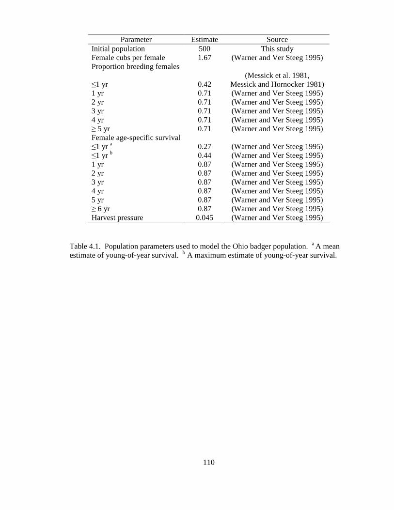
110

Table 4.1. Population parameters used to model the Ohio badger population. a A mean estimate of young-of-year survival. b A maximum estimate of young-of-year survival.

Parameter Estimate Source Initial population 500 This study Female cubs per female 1.67 (Warner and Ver Steeg 1995) Proportion breeding females

≤1 yr 0.42 (Messick et al. 1981,

Messick and Hornocker 1981) 1 yr 0.71 (Warner and Ver Steeg 1995) 2 yr 0.71 (Warner and Ver Steeg 1995) 3 yr 0.71 (Warner and Ver Steeg 1995) 4 yr 0.71 (Warner and Ver Steeg 1995) ≥ 5 yr 0.71 (Warner and Ver Steeg 1995) Female age-specific survival ≤1 yr a 0.27 (Warner and Ver Steeg 1995) ≤1 yr b 0.44 (Warner and Ver Steeg 1995) 1 yr 0.87 (Warner and Ver Steeg 1995) 2 yr 0.87 (Warner and Ver Steeg 1995) 3 yr 0.87 (Warner and Ver Steeg 1995) 4 yr 0.87 (Warner and Ver Steeg 1995) 5 yr 0.87 (Warner and Ver Steeg 1995) ≥ 6 yr 0.87 (Warner and Ver Steeg 1995) Harvest pressure 0.045 (Warner and Ver Steeg 1995)

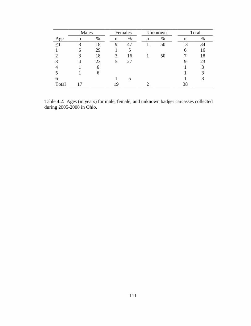
111

Table 4.2. Ages (in years) for male, female, and unknown badger carcasses collected during 2005-2008 in Ohio.

Males Females Unknown Total Age n % n % n % n % ≤1 3 18 9 47 1 50 13 34 1 5 29 1 5 6 16 2 3 18 3 16 1 50 7 18 3 4 23 5 27 9 23 4 1 6 1 3 5 1 6 1 3 6 1 5 1 3 Total 17 19 2 38

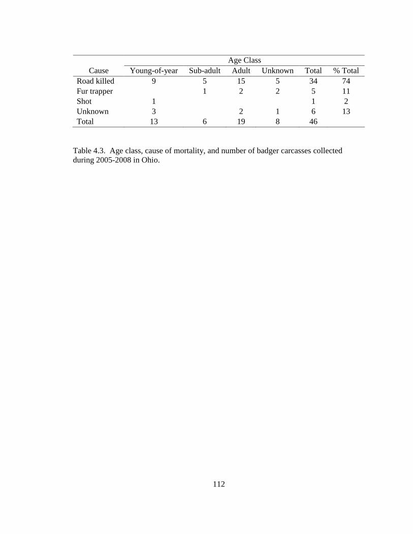
112

Table 4.3. Age class, cause of mortality, and number of badger carcasses collected during 2005-2008 in Ohio.

Age Class Cause Young-of-year Sub-adult Adult Unknown Total % Total

Road killed 9 5 15 5 34 74 Fur trapper 1 2 2 5 11 Shot 1 1 2 Unknown 3 2 1 6 13 Total 13 6 19 8 46

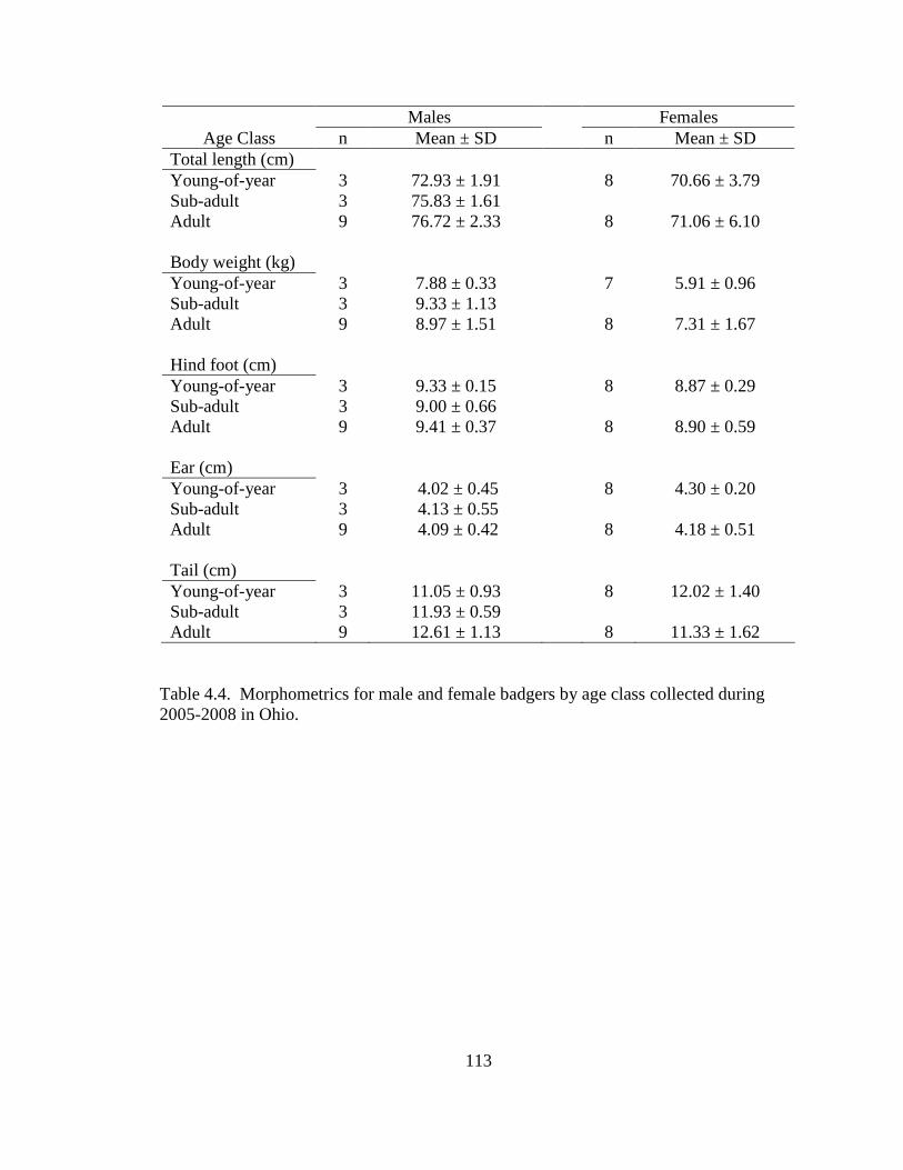
113

Males Females Age Class n Mean ± SD n Mean ± SD

Total length (cm) Young-of-year 3 72.93 ± 1.91 8 70.66 ± 3.79 Sub-adult 3 75.83 ± 1.61 Adult 9 76.72 ± 2.33 8 71.06 ± 6.10 Body weight (kg) Young-of-year 3 7.88 ± 0.33 7 5.91 ± 0.96 Sub-adult 3 9.33 ± 1.13 Adult 9 8.97 ± 1.51 8 7.31 ± 1.67 Hind foot (cm) Young-of-year 3 9.33 ± 0.15 8 8.87 ± 0.29 Sub-adult 3 9.00 ± 0.66 Adult 9 9.41 ± 0.37 8 8.90 ± 0.59 Ear (cm) Young-of-year 3 4.02 ± 0.45 8 4.30 ± 0.20 Sub-adult 3 4.13 ± 0.55 Adult 9 4.09 ± 0.42 8 4.18 ± 0.51 Tail (cm) Young-of-year 3 11.05 ± 0.93 8 12.02 ± 1.40 Sub-adult 3 11.93 ± 0.59 Adult 9 12.61 ± 1.13 8 11.33 ± 1.62

Table 4.4. Morphometrics for male and female badgers by age class collected during 2005-2008 in Ohio.

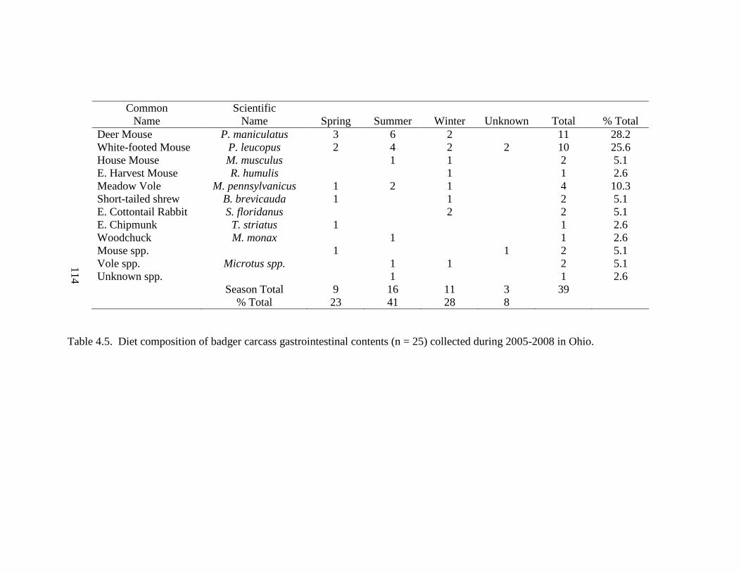
125

Common Name

Scientific Name Spring Summer Winter Unknown Total % Total

Deer Mouse P. maniculatus 3 6 2 11 28.2 White-footed Mouse P. leucopus 2 4 2 2 10 25.6 House Mouse M. musculus 1 1 2 5.1 E. Harvest Mouse R. humulis 1 1 2.6 Meadow Vole M. pennsylvanicus 1 2 1 4 10.3 Short-tailed shrew B. brevicauda 1 1 2 5.1 E. Cottontail Rabbit S. floridanus 2 2 5.1 E. Chipmunk T. striatus 1 1 2.6 Woodchuck M. monax 1 1 2.6 Mouse spp. 1 1 2 5.1 Vole spp. Microtus spp. 1 1 2 5.1 Unknown spp. 1 1 2.6 Season Total 9 16 11 3 39 % Total 23 41 28 8

Table 4.5. Diet composition of badger carcass gastrointestinal contents (n = 25) collected during 2005-2008 in Ohio.

114

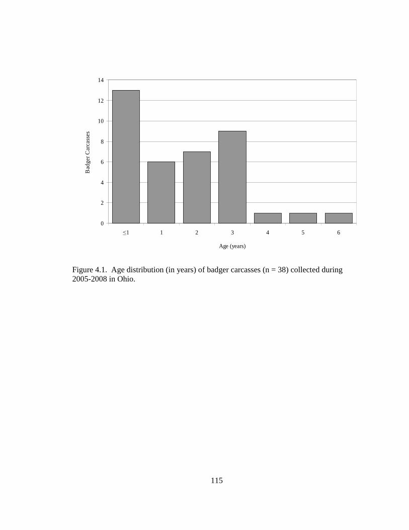
115

0

2

4

6

8

10

12

14

≤1 1 2 3 4 5 6

Age (years)

Bad

ger

Car

cass

es

Figure 4.1. Age distribution (in years) of badger carcasses (n = 38) collected during 2005-2008 in Ohio.

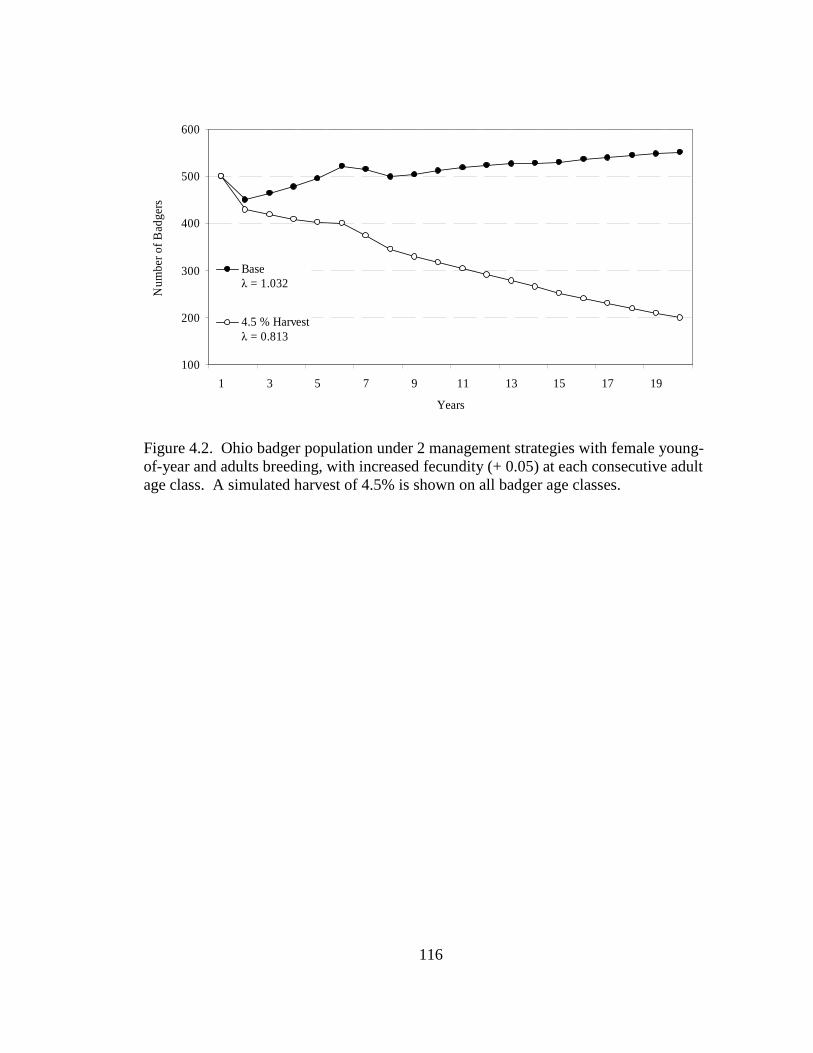
116

100

200

300

400

500

600

1 3 5 7 9 11 13 15 17 19

Years

Nu

mbe

r o

f Bad

gers

Base λ = 1.032

4.5 % Harvestλ = 0.813

Figure 4.2. Ohio badger population under 2 management strategies with female young-of-year and adults breeding, with increased fecundity (+ 0.05) at each consecutive adult age class. A simulated harvest of 4.5% is shown on all badger age classes.

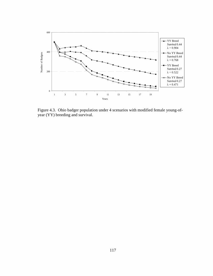
117

0

200

400

600

1 3 5 7 9 11 13 15 17 19

Years

Num

ber

of B

adge

rsYY BreedSurvival 0.44 λ = 0.904

No YY BreedSurvival 0.44 λ = 0.768

YY BreedSurvival 0.27 λ = 0.522

No YY BreedSurvival 0.27 λ = 0.471

Figure 4.3. Ohio badger population under 4 scenarios with modified female young-of-year (YY) breeding and survival.

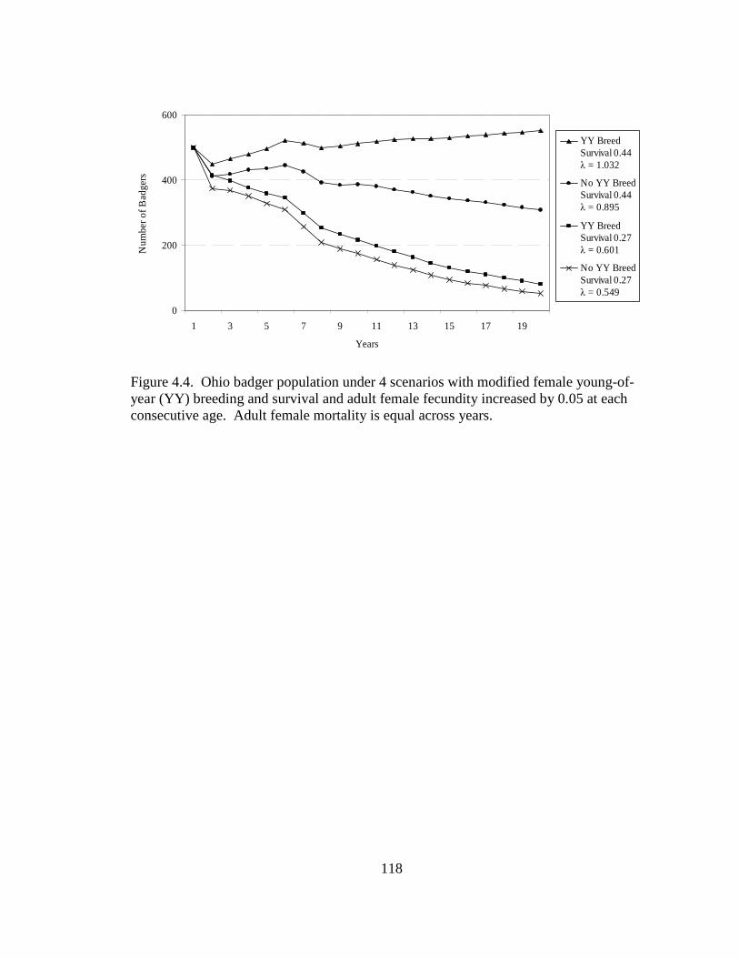
118

0

200

400

600

1 3 5 7 9 11 13 15 17 19

Years

Num

ber

of B

adge

rsYY BreedSurvival 0.44 λ = 1.032

No YY BreedSurvival 0.44 λ = 0.895

YY BreedSurvival 0.27 λ = 0.601

No YY BreedSurvival 0.27 λ = 0.549

Figure 4.4. Ohio badger population under 4 scenarios with modified female young-of-year (YY) breeding and survival and adult female fecundity increased by 0.05 at each consecutive age. Adult female mortality is equal across years.

119

BIBLIOGRAPHY Aebischer, N.J., P.A. Robertson, and R.E. Kenward. 1993. Compositional analysis of habitat use from animal radio-tracking data. Ecology 74: 1313-1323. Apps, C.D., B.N. McLellan, J.G. Woods, and M.F. Proctor. 2004. Estimating grizzly bear distribution and abundance relative to habitat and human influence. Journal of Wildlife Management 68: 138-152. Apps, C.D., N.J. Newhouse, and T.A. Kinley. 2002. Habitat associations of American badgers in southeastern British Columbia. Aspinall, R.J., G. Burton, and L. Landenburger. 1998. Mapping and modelling wildlife species distribution for biodiversity management. In: Proceedings of the 18th Annual ESRI International User, San Diego, California. Available online:http://gis2.esri.com/library/userconf/proc98/PROCEED/TO800/PAP783/P 783.HTM. Azevedo, F.C.C., V. Lester, W. Gorsuch, S. Lariviere, A.J. Wirsing, and D.L. Murray. 2006. Dietary breadth and overlap among five sympatric prairie carnivores. Journal of Zoology 269: 127-135. Berkley, K.A., and S.A. Johnson. 1998. Range expansion of the badger (Taxidea taxus) in Indiana. Proceedings of the Indiana Academy of Science 107: 141-150. Beyer, H. L. 2004. Hawth's Analysis Tools for ArcGIS. <http://www.spatialecology.com/htools>. Accessed 15 Sep 2006. Bowers, M.A., and J.L. Dooley, Jr. 1999. A controlled, hierarchical study of habitat fragmentation: responses at the individual, patch, and landscape scale. Landscape Ecology 14: 381-389. Brown, J.H. 1984. On the relationship between abundance and distribution of species. American Naturalist 124: 255-279. Burnham, K.P., and D.R. Anderson. 2002. Model selection and multimodel inference. Second edition. Springer, New York, USA. Burt, W.H. 1943. Territoriality and home range concepts as applies to mammals. Journal of Mammalogy 24: 346-352.

120

Carroll, C., R.F. Noss, P.C. Paquet, and N.H. Schumaker. 2003. Use of population viability analysis and reserve selection algorithms in regional conservation plans. Ecological Applications 13: 1773-1789. Cherkassky, V., and Y. Ma. 2003. Comparison of model selection for regression. Neural Computation 15: 1691-1714. Clark, J.D., J.E. Dunn, and K.G. Smith. 1993. A multivariate model of female black bear habitat use for a GIS. Journal of Wildlife Management 57: 519-526. Clarke, G. P., P.C.L. White, and S. Harris. 1998. Effects of roads on badger Meles meles populations in south-west England. Biological Conservation 86: 117-124. Cleveland, E.D. 1985. The southernmost record of the badger (Taxidea taxus) in Kansas. Transactions of the Kansas Academy of Science 88: 144-145. Crooks, K.R. 2002. Relative sensitivities of mammalian carnivores to habitat fragmentation. Conservation Biology 16: 488-502. Crowe, D.M., and M.D. Strickland. 1975. Dental annulation in the American badger. Journal of Mammalogy 56: 269-272. Daley, J.G. 1992. Population reductions and genetic variability in black-tailed prairie dogs. Journal of Wildlife Management 56: 212-220. Dettmers, R., and J. Bart. 1999. A GIS modeling method applied to predicting forest songbird habitat. Ecological Applications 9: 152-163. Dijak, W.D., and F.R. Thompson. 2000. Landscape and edge effects on the distribution of mammalian predators in Missouri. Journal of Wildlife Management 64: 209- 216. Environmental Systems Research Institute, Inc. 2008. ArcGIS 9.1. Redlands, CA. Errington, P.L. 1937. Summer food habits of the badger in northwestern Iowa. Journal of Mammalogy 18: 213-216. Freese, C.H., K.E. Aune, D.P. Boyd, J.N. Derr, S.C. Forrest, C.C. Gates, P.J.P. Gogan, S.M. Grassel, N.D. Halbert, K. Kunkel, and K.H. Redford. 2007. Second chance for the plains bison. Biological Conservation 136: 175-184. Fuhlendorf, S.D, A.J.W. Woodward, D.M. Leslie, and J.S. Shackford. 2002. Multi-scale effects of habitat loss and fragmentation on lesser prairie-chicken populations of the US southern Great Plains. Landscape Ecology 17: 617-628.

121

Gaston, K.J., and J.H. Lawton. 1990. Effects of scale and habitat on the relationship between regional distribution and local abundance. Oikos 58: 329-335. Gehring, T.M., and R.K. Swihart. 2004. Home range and movements of long-tailed

weasels in a landscape fragmented by agriculture. Journal of Mammalogy 85: 79-86.

Gese, E.M. 2001. Monitoring of terrestrial carnivore populations. In: Gittleman JL, SM Funk, D MacDonald & RK Wayne (eds) Carnivore conservation: 372-396. Cambridge University Press, Cambridge, United Kingdom. Gittleman, J.L., and P.H. Harvey. 1982. Carnivore home-range size, metabolic needs

and ecology. Behavioral Ecology and Sociobiology 10: 57-63. Gompper, M.E., R.W. Kays, J.C. Ray, S.D. Lapoint, D.A. Bogan, and J.R. Cryan. 2006. A comparison of noninvasive techniques to survey carnivore communities in northeastern North America. Wildlife Society Bulletin 34: 1142-1151. Goodrich, J.M., and S.W. Buskirk. 1998. Spacing and ecology of North American badgers (Taxidea taxus) in a prairie-dog (Cynomys leucurus) complex. Journal of Mammalogy 79: 171-179. Gordon, R.B. 1966. Original vegetation of Ohio at the time of the earliest land surveys. Ohio Biological Survey, Columbus, Ohio. Gosselink, T.E., T.R. Van Deelen, R.E. Warner, and P.C. Mankin. 2007. Survival and cause-specific mortality of red foxes in agricultural and urban areas of Illinois. Journal of Wildlife Management 71: 1862-1873. Gremillion-Smith, C. 1985. Range extension of the badger (Taxidea taxus) in southern Illinois. Transactions of the Illinois Academy of Science 78: 111-114. Haddad, N.M., D.R. Bowne, A. Cunningham, B.J. Danielson, D.J. Levey, S. Sargent, and T. Spira. 2003. Corridor use by diverse taxa. Ecology 84: 609-615. Heske, E.J. 1995. Mammalian abundances on forest-farm edges versus forest interiors in southern Illinois: is there an edge effect? Journal of Mammalogy 76: 562-568. Hilty, J.A., and A.M. Merenlender. 2004. Use of riparian corridors and vineyards by mammalian predators in northern California. Conservation Biology 18: 126-135. Hine, J.S. 1906. Notes on some Ohio mammals. The Ohio Naturalist 6: 550-551. Hoodicoff, C.S. 2003. Ecology of the badger (Taxidea taxus jeffersoni) in the Thompson region of British Columbia: implications for conservation. M.S. Thesis. University of Victoria, Victoria. 111pp.

122

Hoving, C.L., D.J. Harrison, W.B. Krohn, R.A. Joseph, and M. O’Brien. 2005. Broad- scale predictors of Canada lynx occurrence in eastern North America. Journal of Wildlife Management 69: 739-751. Illinois Department of Natural Resources. 1996. Illinois Natural Resources Geospatial Data Clearinghouse. Illinois Natural History Survey. 2003. Illinois GAP program data. IUCN 2008. 2008 IUCN Red List of Threatened Species. <www.iucnredlist.org>. Accessed 11 August 2008. Jannett, Jr., F.J., M.R. Broschart, L.H. Grim, and J.P. Schaberl. 2007. Northerly range extensions of mammalian species in Minnesota. American Midland Naturalist 158: 168-176. Jense, G.K. 1968. Food habits and energy utilization of badgers. M.S. Thesis. South Dakota State University, Brookings. 47pp. Johnson, D.H. 1980. The comparison of usage and availability measurements for evaluating resource preference. Ecology 61: 65-71. Kamler, J.F., W.B. Ballard, E.B. Fish, P.R. Lemons, K. Mote, and C.C. Perchellet. 2003. Habitat use, home ranges, and survival of swift foxes in a fragmented landscape: conservation implications. Journal of Mammalogy 84: 989-995. Katnik, D.D., and R.B. Wielgus. 2005. Landscape proportions versus monte carlo simulated home ranges for estimating habitat availability. Journal of Wildlife Management 69: 20- 32. Kaufman, D.W., B.K. Clark, and G.A. Kaufman. 1990. Habitat breadth of nongame rodents in the mixed-grass prairie region of north central Kansas. Prairie Naturalist 22: 19-26. Kays, R.W., M.E. Gompper, and J.C. Ray. 2008. Landscape ecology of eastern coyotes based on large-scale estimates of abundance. Ecological Applications 18: 1014- 1027. Kellert, S.R., M. Black, C.R. Rush, and A.J. Bath. 1996. Human culture and large carnivore conservation in North America. Conservation Biology 10: 977-990. Kernohan, B.J., J. J. Millspaugh, J. A. Jenks, and D. E. Naugle. 1998. Use of an adaptive kernel home-range estimator in a GIS environment to calculate habitat use. Journal of Environmental Management 53: 83-89.

123

Laliberte, A.S., and W.J. Ripple. 2004. Range contractions of North American carnivores and ungulates. BioScience 54: 123-138. Lampe, R.P. 1976. Aspects of the predatory strategy of the North American badger (Taxidea taxus). Ph.D. Dissertation. University of Minnesota, St. Paul. 106pp. Lampe, R.P. 1982. Food habits of badger in east central Minnesota. Journal of Wildlife Management 46: 790-795. Lampe, R.P., and M.A. Sovada. 1981. Seasonal variation in home range of a female badger (Taxidea taxus). The Prairie Naturalist 13: 55-58. Leedy, D.L. 1947. Spermophiles and badgers move eastward in Ohio. Journal of Mammalogy 28: 290-292. Levin, S.A. 1992. The problem of pattern and scale in ecology: The Robert H. MacArthur Award Lecture. Ecology 73: 1943-1967. Lindstedt, S.L., B.J. Miller, and S.W. Buskirk. 1986. Home range, time, and body size

in mammals. Ecology 67: 413-418. Lindzey, F.G. 1971. Ecology of badgers in Curlew Valley, Utah and Idaho with emphasis on movement and activity patterns. M.S. Thesis. Utah State University, Logan. 50pp. Lindzey, F.G. 1978. Movement patterns of badgers in northwestern Utah. Journal of Wildlife Management 42: 418-422. Lintack, W.M., and D.R. Voigt. 1983. Distribution of the Badger, Taxidea taxus, in southwestern Ontario. Canadian Field-Naturalist 97: 107-109. Long, C.A. 1972. Taxonomic revision of the North American badger, Taxidea taxus. Journal of Mammalogy 53: 725-759. Long, C.A., and C.A. Killingley. 1983. The badgers of the world. Charles C. Thomas Publishers, Springfield, Illinois. 404pp. Lyon, M.W., Jr. 1932. The badger Taxidea taxus (Schreber), in Indiana. American Midland Naturalist 13: 124-129. Manly, B. F. 2005. Multivariate statistical methods: a primer. Third edition. Chapman and Hall/CRC Press, Boca Raton, Florida, USA. Manly, B.F., J.L.L. McDonald, D.L. Thomas, T.L McDonald, and W.P. Erickson. 2002. Resource selection by animals: statistical design and analysis for field studies. Second edition. Kluwer Academic Publishers, Boston, Massachusetts, USA.

124

McGarigal, K., and B.J. Marks. 1995. FRAGSTATS: spatial pattern analysis program for quantifying landscape structure. Version 3.3. United States Forest Service General Technical Report PNW-GTR-351, Portland, Oregon, USA. Messick, J.P. 1999. North American Badger. Pages 586-597 in Wild Furbearer

Management and Conservation in North America. Messick, J.P., and M.G. Hornocker. 1981. Ecology of the badger in southwestern Idaho. Wildlife Monographs 76. 56pp. Messick, J.P., M.C. Todd, and M.G. Hornocker. 1981. Comparative ecology of two badger populations. Pp. 1290-1304, in Proceeding of the worldwide furbearer conference (J. Chapman and D. Pursley, eds.). International Association of Fish and Wildlife Agencies, Washington, D.C., 1451 pp. Meunier, F.D., J. Corbin, C. Verheyden, and P. Jouventin. 1999. Effects of landscape type and extensive management on use of motorway roadsides by small mammals. Canadian Journal of Zoology 77: 108-117. Mills, L.S. 2007. Conservation of wildlife populations: demography, genetics, and management. Blackwell Publishing, Malden, MA. 407pp. Minta, S.C. 1993. Sexual differences in spatiotemporal interaction among badgers. Oecologia 96: 402-409. Minta, S.C., and R.E. Marsh. 1988. Badgers (Taxidea taxus) as occasional pests in agriculture. Proceedings of the Vertebrate Pest Conference 13: 199-208. Mohr, C.O. 1947. Table of equivalent populations of North American small mammals. American Midland Naturalist 37: 223-249. Morris, D.W. 1987. Ecological scale and habitat use. Ecology 68: 362-369. Moseley, E.L. 1934. Increase of badgers in northwestern Ohio. Journal of Mammalogy 15: 156-158. Mumford, R.E., and J.O. Whitaker, Jr. 1982. Mammals of Indiana. Indiana University Press, Bloomington, Indiana. Newhouse, N.J., and T.A. Kinley. 2000. Ecology of American badgers near their range limit in southeastern British Columbia. Unpublished Report. Columbia Basin Fish and Wildlife Compensation Program, Nelson, and Parks Canada, Radium Hot Springs, British Columbia. Nielsen, C. K., and A. Woolf. 2002. Habitat-relative abundance relationship for bobcats in southern Illinois. Wildlife Society Bulletin 30:222–230.

125

Northern Prairie Science Center. 1994. Program PREFER. Version 5.1. <http://www.npwrc.usgs.gov/resource/methods/prefer/index.htm>. Accessed 1 Dec 2006. Noss, R.F., H.B. Quigley, M.G. Hornocker, T. Merrill, and P.C. Paquet. 1996. Conservation biology and carnivore conservation in the Rocky Mountains. Conservation Biology 10: 949-963. Nugent, R.F., and J.R. Choate. 1970. Eastward dispersal of the badger, Taxidea taxus, into the northeastern United States. Journal of Mammalogy 51: 626-627. Ohio Department of Development, Office of Strategic Research. 2000. Ohio County Profiles. Appendix B: Sources. Land Cover. Ohio Division of Forestry. 2008. History of Ohio Forests. <http://www.dnr.state.oh.us/tabid/5225/Default.aspx>. Accessed 20 Jul 2008. Ohio Division of Natural Areas and Preserves. 2008. Ohio Prairies. <http://www.dnr.state.oh.us/tabid/1979/Default.aspx>. Accessed 20 Jul 2008. Packham, R.M., and C.S. Hoodicoff. 2004. Badger ecology in the Cariboo region of British Columbia, Canada. Proceedings of the Species at Risk 2004 Pathways to Recovery Conference. Victoria, British Columbia. Palma, L., P. Beja, and M. Rodrigues. 1999. The use of sighting data to analyse Iberian lynx habitat and distribution. Journal of Applied Ecology 36: 812-824. Preuss, T.S., and T.M. Gehring. 2007. Landscape analysis of bobcat habitat in the northern lower peninsula of Michigan. Journal of Wildlife Management 71: 2699-2706. Pyare, S., S. Cain, D. Moody, C. Schwartz, and J. Berger. 2004. Carnivore re- colonization: reality, possibility and a non-equilibrium century for grizzly bears in the southern yellowstone ecosystem. Animal Conservation 7: 71-77. R Development Core Team. 2006. R: a language and environment for statistical computing. R Foundation for Statistical Computing, Vienna, Austria. Radeloff, V.C., R.B. Hammer, and S.I. Stewart. 2005. Rural and surburban sprawl in the U.S. Midwest from 1940 to 2000 and its relation to forest fragmentation. Conservation Biology 19: 793-805. Ray, J.C. 2000. Mesocarnivores of northeastern North America: status and conservation issues. Wildlife Conservation Society Working Paper 15: 1–82.

126

Rodgers, A.R., A.P. Carr, H.L. Beyer, L. Smith, and J.G. Kie. 2007. HRT: Home Range Tools for ArcGIS. Version 1.1. Ontario Ministry of Natural Resources, Centre for Northern Forest Ecosystem Research, Thunder Bay, Ontario, Canada. Rosalino, L. M., M.J. Santos, S. Domingos, M. Rodrigues, and M. Santos-Reis. 2005. Population structure and body size of sympatric carnivores in a mediterranean landscape of sw Portugal. Revista de Biologia 23: 135-146. Ryall, K.L., and L. Fahrig. 2006. Response of predators to loss and fragmentation of prey habitat: a review of theory. Ecology 87: 1086-1093. Sacks, B.N. 2005. Reproduction and body condition of California coyotes (Canis latrans). Journal of Mammalogy 86: 1036-1041. Saunders, D.A., R.J. Hobbs, and C.R. Margules. 1991. Biological consequences of ecosystem fragmentation: a review. Conservation Biology 5: 18-32. Schwartz, C.W., and E.R. Schwartz. 1981. The wild mammals of Missouri. University of Missouri Press, Columbia. Seaman, D. E., J.J. Millspaugh, B.J. Kernohan, G.C. Brundige, K.J. Raedeke, and R.A. Gitzen. 1999. Effects of sample size on kernel home range estimates. Journal of Wildlife Management 63: 739-747. Smith, H.G., R.K. Burnard, E.E. Good, and J.M. Keener. 1973. Rare and endangered vertebrates of Ohio. The Ohio Journal of Science 73: 257-271. Snead, I.E., and G.O. Hendrickson. 1942. Food habits of the badger in Iowa. Journal of Mammalogy 23: 380-391. Snyder, E.J., and L.B. Best. 1988. Dynamics of habitat use by small mammals in prairie communities. American Midland Naturalist 119: 128-136. Sovada, M.A., J.M. Roaldson, and A.B. Sargeant. 1999. Foods of American badgers in west-central Minnesota and southern North Dakota during the duck nesting season. American Midland Naturalist 142: 410-415. Swihart, R.K., and N.A. Slade. 1985. Testing for independence of observations in animal movements. Ecology 66: 1176-1184. The Ohio State University, Center for Mapping. 2005. Ohio GAP program land cover data. Todd, M. 1980. Ecology of badgers in southcentral Idaho, with additional notes on raptors. M.S. Thesis. University of Idaho, Moscow. 164pp.

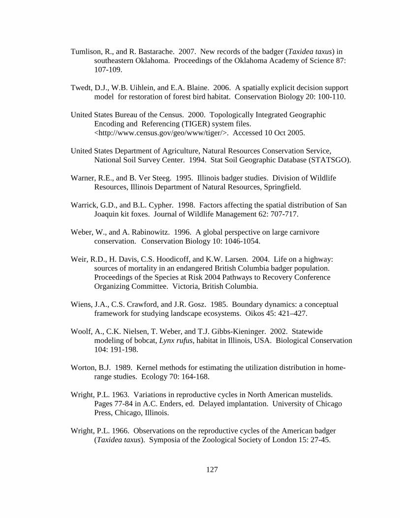
127

Tumlison, R., and R. Bastarache. 2007. New records of the badger (Taxidea taxus) in southeastern Oklahoma. Proceedings of the Oklahoma Academy of Science 87: 107-109. Twedt, D.J., W.B. Uihlein, and E.A. Blaine. 2006. A spatially explicit decision support model for restoration of forest bird habitat. Conservation Biology 20: 100-110. United States Bureau of the Census. 2000. Topologically Integrated Geographic Encoding and Referencing (TIGER) system files. <http://www.census.gov/geo/www/tiger/>. Accessed 10 Oct 2005. United States Department of Agriculture, Natural Resources Conservation Service, National Soil Survey Center. 1994. Stat Soil Geographic Database (STATSGO). Warner, R.E., and B. Ver Steeg. 1995. Illinois badger studies. Division of Wildlife Resources, Illinois Department of Natural Resources, Springfield. Warrick, G.D., and B.L. Cypher. 1998. Factors affecting the spatial distribution of San Joaquin kit foxes. Journal of Wildlife Management 62: 707-717. Weber, W., and A. Rabinowitz. 1996. A global perspective on large carnivore conservation. Conservation Biology 10: 1046-1054. Weir, R.D., H. Davis, C.S. Hoodicoff, and K.W. Larsen. 2004. Life on a highway: sources of mortality in an endangered British Columbia badger population. Proceedings of the Species at Risk 2004 Pathways to Recovery Conference Organizing Committee. Victoria, British Columbia. Wiens, J.A., C.S. Crawford, and J.R. Gosz. 1985. Boundary dynamics: a conceptual framework for studying landscape ecosystems. Oikos 45: 421–427. Woolf, A., C.K. Nielsen, T. Weber, and T.J. Gibbs-Kieninger. 2002. Statewide modeling of bobcat, Lynx rufus, habitat in Illinois, USA. Biological Conservation 104: 191-198. Worton, B.J. 1989. Kernel methods for estimating the utilization distribution in home- range studies. Ecology 70: 164-168. Wright, P.L. 1963. Variations in reproductive cycles in North American mustelids. Pages 77-84 in A.C. Enders, ed. Delayed implantation. University of Chicago Press, Chicago, Illinois. Wright, P.L. 1966. Observations on the reproductive cycles of the American badger (Taxidea taxus). Symposia of the Zoological Society of London 15: 27-45.

128

Zielinski, W.J. 1997. Monitoring mesocarnivore population status. In mesocarnivores of northern California: biology management and survey techniques: 109–115. Harris, J.E. & Ogan, C.V. (Eds). Wildlife Society, Humbolt State University, Arcata. Zielinski, W.J., R.L Truex, F.V. Schlexer, L.A. Campbell, and C. Carroll. 2005. Historical and contemporary distributions of carnivores in forests of the Sierra Nevada, California, USA. Journal of Biogeography 32: 1385-1407.

129

Appendix A. Badger observation poster, originally 11” X 14”, used to opportunistically collect badger reports in Ohio from 2005-2008. Lower left corner of poster shows image of pre-paid tear-off cards placed on posters which allowed observers to send in their report.

130

Appendix B. Fur harvester inquiry used in 2006 to obtain reports of badger observations and captures in Ohio.

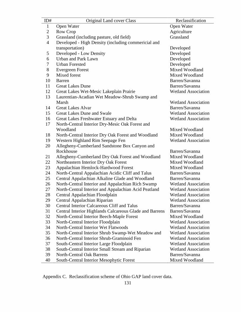
131

Appendix C. Reclassification scheme of Ohio GAP land cover data.

ID# Original Land cover Class Reclassification 1 Open Water Open Water 2 Row Crop Agriculture 3 Grassland (including pasture, old field) Grassland 4 Developed - High Density (including commericial and

transportation) Developed 5 Developed - Low Density Developed 6 Urban and Park Lawn Developed 7 Urban Forested Developed 8 Evergreen Forest Mixed Woodland 9 Mixed forest Mixed Woodland 10 Barren Barren/Savanna 11 Great Lakes Dune Barren/Savanna 12 Great Lakes Wet-Mesic Lakeplain Prairie Wetland Association 13 Laurentian-Acadian Wet Meadow-Shrub Swamp and

Marsh Wetland Association 14 Great Lakes Alvar Barren/Savanna 15 Great Lakes Dune and Swale Wetland Association 16 Great Lakes Freshwater Estuary and Delta Wetland Association 17 North-Central Interior Dry-Mesic Oak Forest and

Woodland Mixed Woodland 18 North-Central Interior Dry Oak Forest and Woodland Mixed Woodland 19 Western Highland Rim Seepage Fen Wetland Association 20 Allegheny-Cumberland Sandstone Box Canyon and

Rockhouse Barren/Savanna 21 Allegheny-Cumberland Dry Oak Forest and Woodland Mixed Woodland 22 Northeastern Interior Dry Oak Forest Mixed Woodland 23 Appalachian Hemlock-Hardwood Forest Mixed Woodland 24 North-Central Appalachian Acidic Cliff and Talus Barren/Savanna 25 Central Appalachian Alkaline Glade and Woodland Barren/Savanna 26 North-Central Interior and Appalachian Rich Swamp Wetland Association 27 North-Central Interior and Appalachian Acid Peatland Wetland Association 28 Central Appalachian Floodplain Wetland Association 29 Central Appalachian Riparian Wetland Association 30 Central Interior Calcareous Cliff and Talus Barren/Savanna 31 Central Interior Highlands Calcareous Glade and Barrens Barren/Savanna 32 North-Central Interior Beech-Maple Forest Mixed Woodland 33 North-Central Interior Floodplain Wetland Association 34 North-Central Interior Wet Flatwoods Wetland Association 35 North-Central Interior Shrub Swamp-Wet Meadow and Wetland Association 36 North-Central Interior Shrub-Graminoid Fen Wetland Association 37 South-Central Interior Large Floodplain Wetland Association 38 South-Central Interior Small Stream and Riparian Wetland Association 39 North-Central Oak Barrens Barren/Savanna 40 South-Central Interior Mesophytic Forest Mixed Woodland

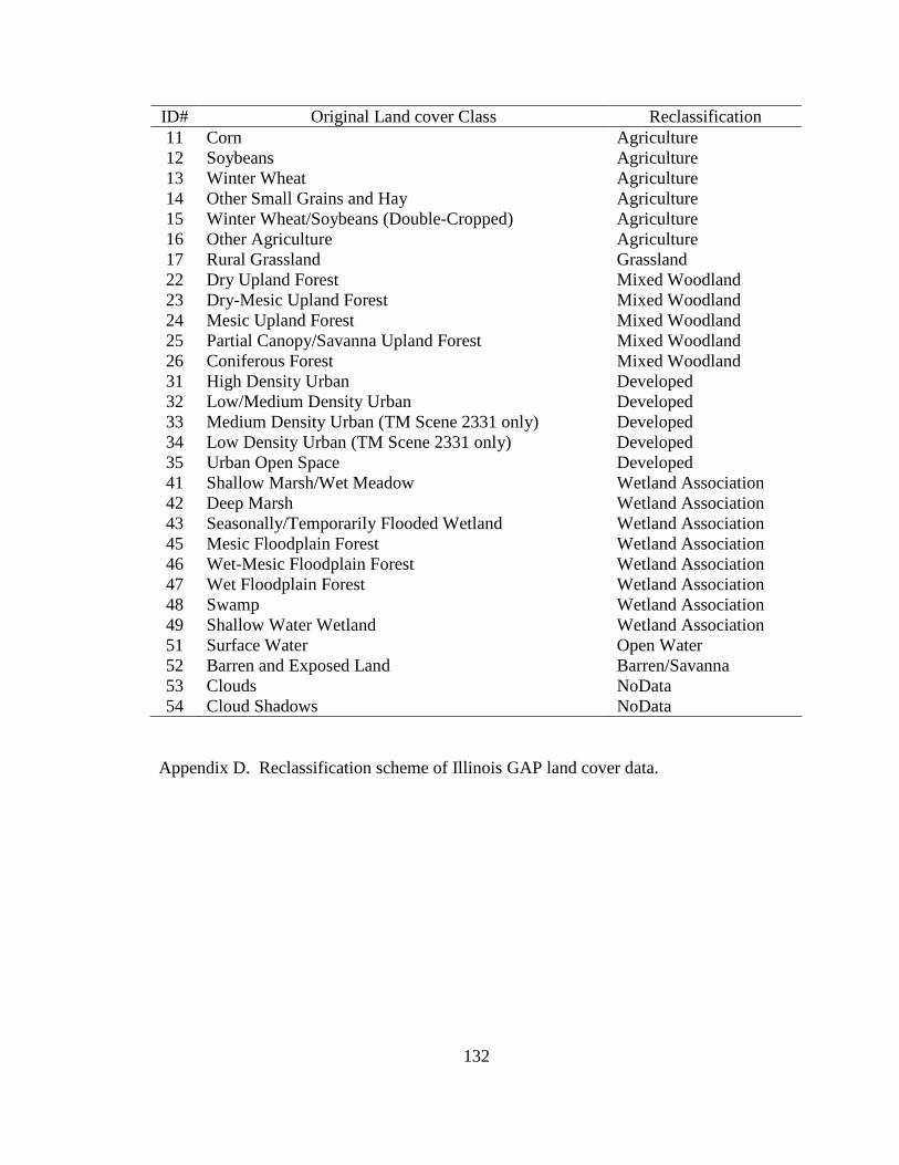
132

ID# Original Land cover Class Reclassification 11 Corn Agriculture 12 Soybeans Agriculture 13 Winter Wheat Agriculture 14 Other Small Grains and Hay Agriculture 15 Winter Wheat/Soybeans (Double-Cropped) Agriculture 16 Other Agriculture Agriculture 17 Rural Grassland Grassland 22 Dry Upland Forest Mixed Woodland 23 Dry-Mesic Upland Forest Mixed Woodland 24 Mesic Upland Forest Mixed Woodland 25 Partial Canopy/Savanna Upland Forest Mixed Woodland 26 Coniferous Forest Mixed Woodland 31 High Density Urban Developed 32 Low/Medium Density Urban Developed 33 Medium Density Urban (TM Scene 2331 only) Developed 34 Low Density Urban (TM Scene 2331 only) Developed 35 Urban Open Space Developed 41 Shallow Marsh/Wet Meadow Wetland Association 42 Deep Marsh Wetland Association 43 Seasonally/Temporarily Flooded Wetland Wetland Association 45 Mesic Floodplain Forest Wetland Association 46 Wet-Mesic Floodplain Forest Wetland Association 47 Wet Floodplain Forest Wetland Association 48 Swamp Wetland Association 49 Shallow Water Wetland Wetland Association 51 Surface Water Open Water 52 Barren and Exposed Land Barren/Savanna 53 Clouds NoData 54 Cloud Shadows NoData

Appendix D. Reclassification scheme of Illinois GAP land cover data.

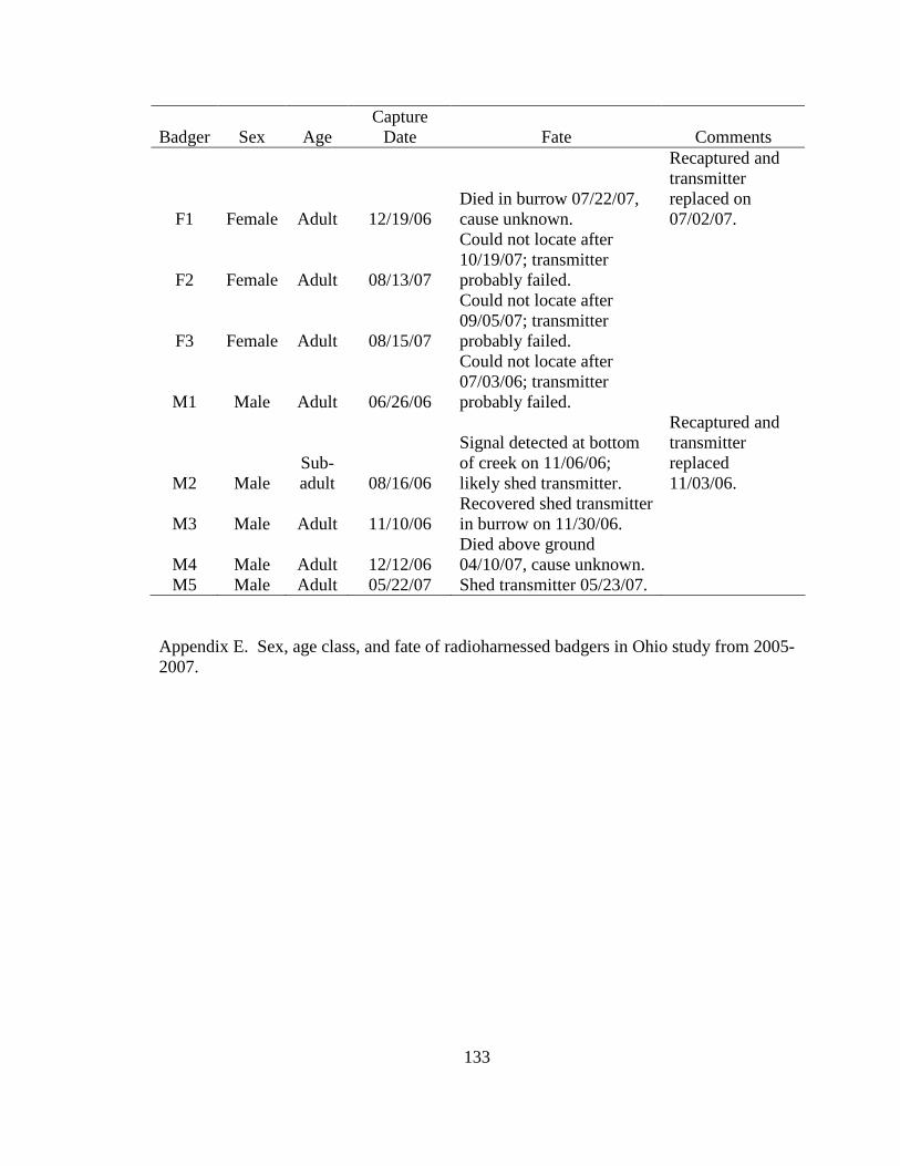
133

Badger

Sex

Age

Capture Date

Fate

Comments

F1 Female Adult 12/19/06 Died in burrow 07/22/07, cause unknown.

Recaptured and transmitter replaced on 07/02/07.

F2 Female Adult 08/13/07

Could not locate after 10/19/07; transmitter probably failed.

F3 Female Adult 08/15/07

Could not locate after 09/05/07; transmitter probably failed.

M1 Male Adult 06/26/06

Could not locate after 07/03/06; transmitter probably failed.

M2 Male Sub-adult 08/16/06

Signal detected at bottom of creek on 11/06/06; likely shed transmitter.

Recaptured and transmitter replaced 11/03/06.

M3 Male Adult 11/10/06 Recovered shed transmitter in burrow on 11/30/06.

M4 Male Adult 12/12/06 Died above ground 04/10/07, cause unknown.

M5 Male Adult 05/22/07 Shed transmitter 05/23/07. Appendix E. Sex, age class, and fate of radioharnessed badgers in Ohio study from 2005-2007.

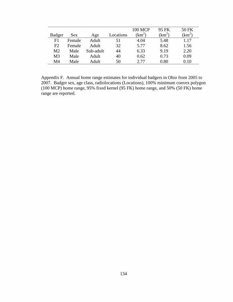
134

Appendix F. Annual home range estimates for individual badgers in Ohio from 2005 to 2007. Badger sex, age class, radiolocations (Locations), 100% minimum convex polygon (100 MCP) home range, 95% fixed kernel (95 FK) home range, and 50% (50 FK) home range are reported.

Badger

Sex

Age

Locations

100 MCP (km2)

95 FK (km2)

50 FK (km2)

F1 Female Adult 51 4.04 5.48 1.17 F2 Female Adult 32 5.77 8.62 1.56 M2 Male Sub-adult 44 6.33 9.19 2.20 M3 Male Adult 40 0.62 0.73 0.09 M4 Male Adult 50 2.77 0.80 0.10

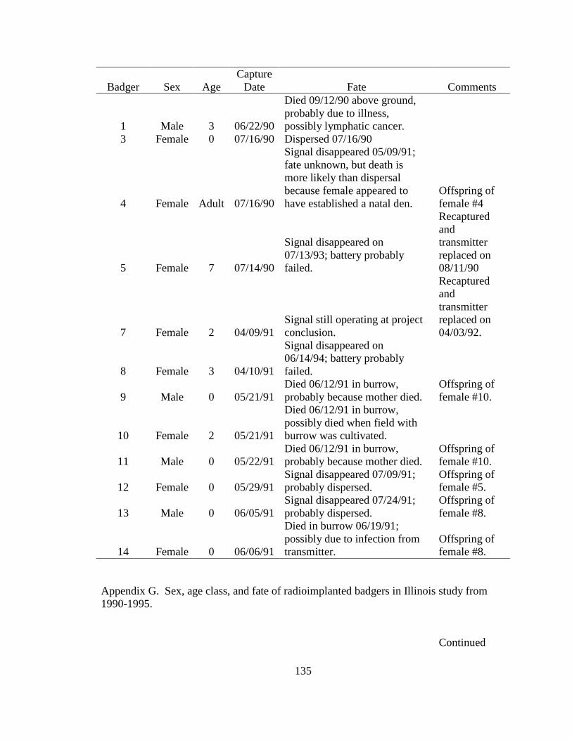
135

Badger

Sex

Age

Capture Date

Fate

Comments

1 Male 3 06/22/90

Died 09/12/90 above ground, probably due to illness, possibly lymphatic cancer.

3 Female 0 07/16/90 Dispersed 07/16/90

4 Female Adult 07/16/90

Signal disappeared 05/09/91; fate unknown, but death is more likely than dispersal because female appeared to have established a natal den.

Offspring of female #4

5 Female 7 07/14/90

Signal disappeared on 07/13/93; battery probably failed.

Recaptured and transmitter replaced on 08/11/90

7 Female 2 04/09/91 Signal still operating at project conclusion.

Recaptured and transmitter replaced on 04/03/92.

8 Female 3 04/10/91

Signal disappeared on 06/14/94; battery probably failed.

9 Male 0 05/21/91 Died 06/12/91 in burrow, probably because mother died.

Offspring of female #10.

10 Female 2 05/21/91

Died 06/12/91 in burrow, possibly died when field with burrow was cultivated.

11 Male 0 05/22/91 Died 06/12/91 in burrow, probably because mother died.

Offspring of female #10.

12 Female 0 05/29/91 Signal disappeared 07/09/91; probably dispersed.

Offspring of female #5.

13 Male 0 06/05/91 Signal disappeared 07/24/91; probably dispersed.

Offspring of female #8.

14 Female 0 06/06/91

Died in burrow 06/19/91; possibly due to infection from transmitter.

Offspring of female #8.

Appendix G. Sex, age class, and fate of radioimplanted badgers in Illinois study from 1990-1995.

Continued

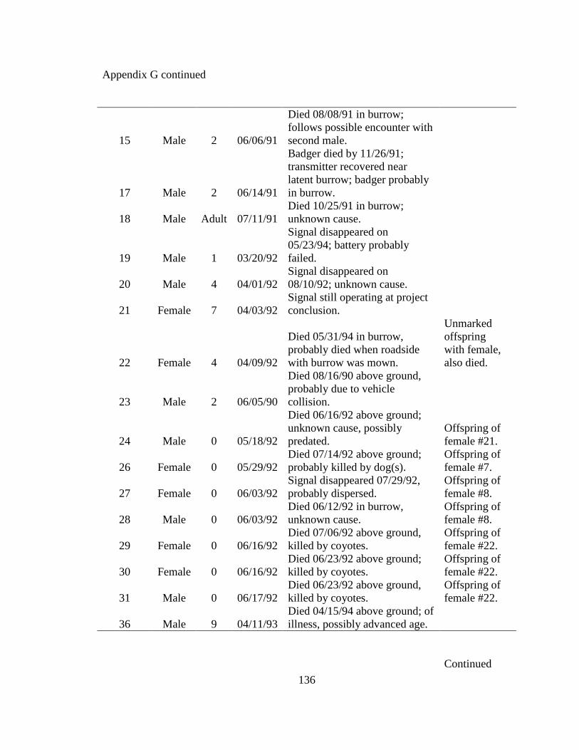
136

Appendix G continued

15 Male 2 06/06/91

Died 08/08/91 in burrow; follows possible encounter with second male.

17 Male 2 06/14/91

Badger died by 11/26/91; transmitter recovered near latent burrow; badger probably in burrow.

18 Male Adult 07/11/91 Died 10/25/91 in burrow; unknown cause.

19 Male 1 03/20/92

Signal disappeared on 05/23/94; battery probably failed.

20 Male 4 04/01/92 Signal disappeared on 08/10/92; unknown cause.

21 Female 7 04/03/92 Signal still operating at project conclusion.

22 Female 4 04/09/92

Died 05/31/94 in burrow, probably died when roadside with burrow was mown.

Unmarked offspring with female, also died.

23 Male 2 06/05/90

Died 08/16/90 above ground, probably due to vehicle collision.

24 Male 0 05/18/92

Died 06/16/92 above ground; unknown cause, possibly predated.

Offspring of female #21.

26 Female 0 05/29/92 Died 07/14/92 above ground; probably killed by dog(s).

Offspring of female #7.

27 Female 0 06/03/92 Signal disappeared 07/29/92, probably dispersed.

Offspring of female #8.

28 Male 0 06/03/92 Died 06/12/92 in burrow, unknown cause.

Offspring of female #8.

29 Female 0 06/16/92 Died 07/06/92 above ground, killed by coyotes.

Offspring of female #22.

30 Female 0 06/16/92 Died 06/23/92 above ground; killed by coyotes.

Offspring of female #22.

31 Male 0 06/17/92 Died 06/23/92 above ground, killed by coyotes.

Offspring of female #22.

36 Male 9 04/11/93 Died 04/15/94 above ground; of illness, possibly advanced age.

Continued

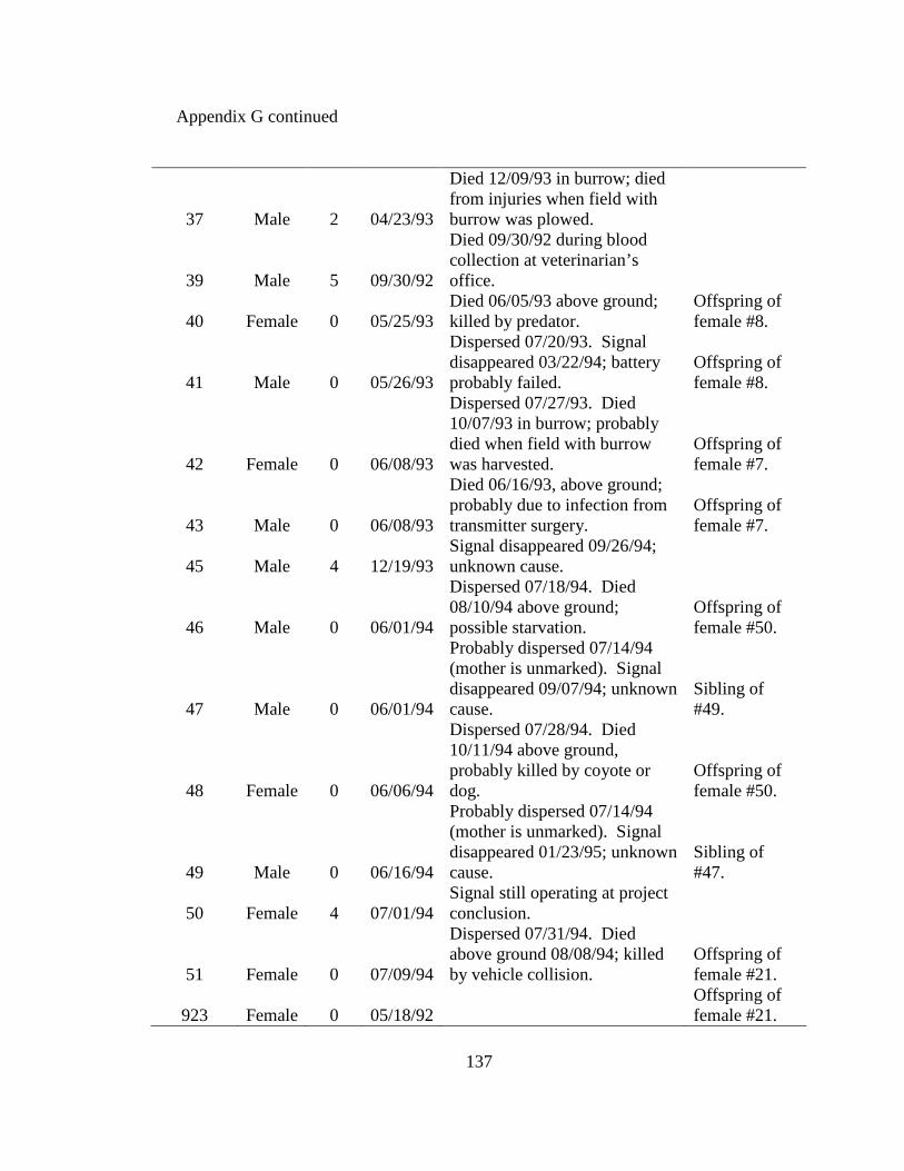
137

Appendix G continued

37 Male 2 04/23/93

Died 12/09/93 in burrow; died from injuries when field with burrow was plowed.

39 Male 5 09/30/92

Died 09/30/92 during blood collection at veterinarian’s office.

40 Female 0 05/25/93 Died 06/05/93 above ground; killed by predator.

Offspring of female #8.

41 Male 0 05/26/93

Dispersed 07/20/93. Signal disappeared 03/22/94; battery probably failed.

Offspring of female #8.

42 Female 0 06/08/93

Dispersed 07/27/93. Died 10/07/93 in burrow; probably died when field with burrow was harvested.

Offspring of female #7.

43 Male 0 06/08/93

Died 06/16/93, above ground; probably due to infection from transmitter surgery.

Offspring of female #7.

45 Male 4 12/19/93 Signal disappeared 09/26/94; unknown cause.

46 Male 0 06/01/94

Dispersed 07/18/94. Died 08/10/94 above ground; possible starvation.

Offspring of female #50.

47 Male 0 06/01/94

Probably dispersed 07/14/94 (mother is unmarked). Signal disappeared 09/07/94; unknown cause.

Sibling of #49.

48 Female 0 06/06/94

Dispersed 07/28/94. Died 10/11/94 above ground, probably killed by coyote or dog.

Offspring of female #50.

49 Male 0 06/16/94

Probably dispersed 07/14/94 (mother is unmarked). Signal disappeared 01/23/95; unknown cause.

Sibling of #47.

50 Female 4 07/01/94 Signal still operating at project conclusion.

51 Female 0 07/09/94

Dispersed 07/31/94. Died above ground 08/08/94; killed by vehicle collision.

Offspring of female #21.

923 Female 0 05/18/92 Offspring of female #21.

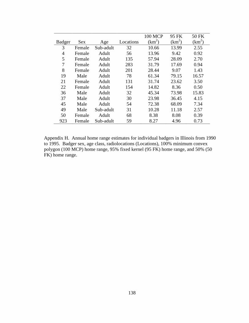
138

Appendix H. Annual home range estimates for individual badgers in Illinois from 1990 to 1995. Badger sex, age class, radiolocations (Locations), 100% minimum convex polygon (100 MCP) home range, 95% fixed kernel (95 FK) home range, and 50% (50 FK) home range.

Badger

Sex

Age

Locations

100 MCP (km2)

95 FK (km2)

50 FK (km2)

3 Female Sub-adult 32 10.66 13.99 2.55 4 Female Adult 56 13.96 9.42 0.92 5 Female Adult 135 57.94 28.09 2.70 7 Female Adult 283 31.79 17.69 0.94 8 Female Adult 201 28.44 9.07 1.43 19 Male Adult 78 61.34 79.15 16.57 21 Female Adult 131 31.74 23.62 3.50 22 Female Adult 154 14.82 8.36 0.50 36 Male Adult 32 45.34 73.98 15.83 37 Male Adult 30 23.98 36.45 4.15 45 Male Adult 54 72.38 68.09 7.34 49 Male Sub-adult 31 10.28 11.18 2.57 50 Female Adult 68 8.38 8.08 0.39 923 Female Sub-adult 59 8.27 4.96 0.73

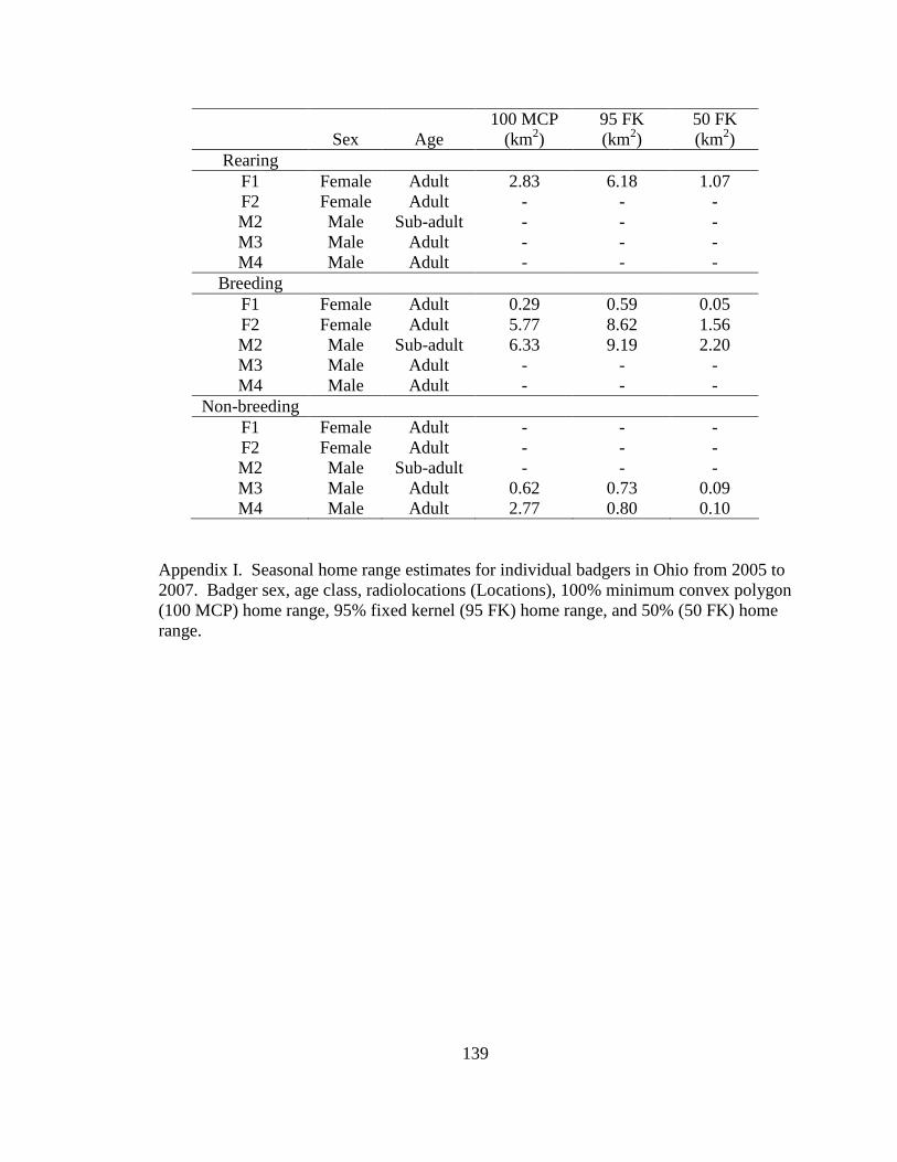
139

Appendix I. Seasonal home range estimates for individual badgers in Ohio from 2005 to 2007. Badger sex, age class, radiolocations (Locations), 100% minimum convex polygon (100 MCP) home range, 95% fixed kernel (95 FK) home range, and 50% (50 FK) home range.

Sex

Age 100 MCP

(km2) 95 FK (km2)

50 FK (km2)

Rearing F1 Female Adult 2.83 6.18 1.07 F2 Female Adult - - - M2 Male Sub-adult - - - M3 Male Adult - - - M4 Male Adult - - -

Breeding F1 Female Adult 0.29 0.59 0.05 F2 Female Adult 5.77 8.62 1.56 M2 Male Sub-adult 6.33 9.19 2.20 M3 Male Adult - - - M4 Male Adult - - -

Non-breeding F1 Female Adult - - - F2 Female Adult - - - M2 Male Sub-adult - - - M3 Male Adult 0.62 0.73 0.09 M4 Male Adult 2.77 0.80 0.10

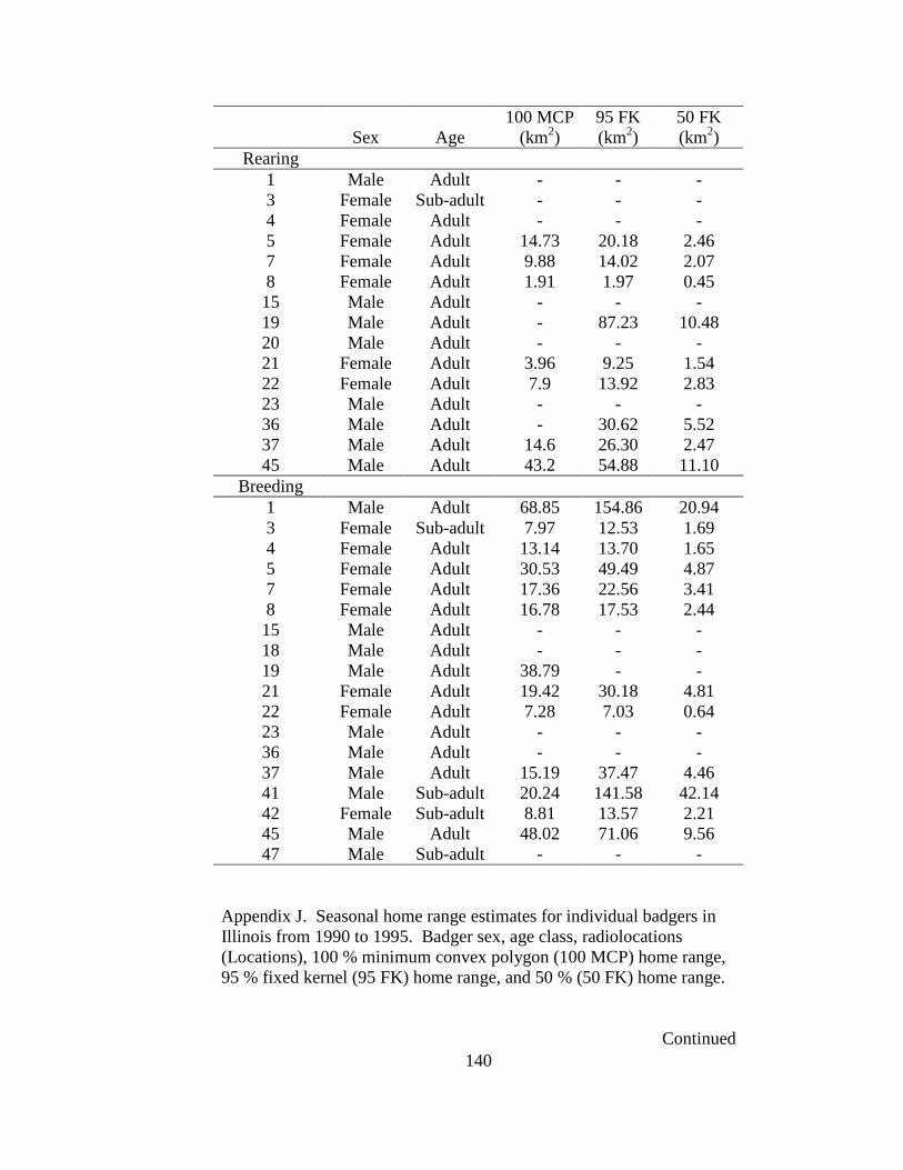
140

Sex

Age 100 MCP

(km2) 95 FK (km2)

50 FK (km2)

Rearing 1 Male Adult - - - 3 Female Sub-adult - - - 4 Female Adult - - - 5 Female Adult 14.73 20.18 2.46 7 Female Adult 9.88 14.02 2.07 8 Female Adult 1.91 1.97 0.45 15 Male Adult - - - 19 Male Adult - 87.23 10.48 20 Male Adult - - - 21 Female Adult 3.96 9.25 1.54 22 Female Adult 7.9 13.92 2.83 23 Male Adult - - - 36 Male Adult - 30.62 5.52 37 Male Adult 14.6 26.30 2.47 45 Male Adult 43.2 54.88 11.10

Breeding 1 Male Adult 68.85 154.86 20.94 3 Female Sub-adult 7.97 12.53 1.69 4 Female Adult 13.14 13.70 1.65 5 Female Adult 30.53 49.49 4.87 7 Female Adult 17.36 22.56 3.41 8 Female Adult 16.78 17.53 2.44 15 Male Adult - - - 18 Male Adult - - - 19 Male Adult 38.79 - - 21 Female Adult 19.42 30.18 4.81 22 Female Adult 7.28 7.03 0.64 23 Male Adult - - - 36 Male Adult - - - 37 Male Adult 15.19 37.47 4.46 41 Male Sub-adult 20.24 141.58 42.14 42 Female Sub-adult 8.81 13.57 2.21 45 Male Adult 48.02 71.06 9.56 47 Male Sub-adult - - -

Appendix J. Seasonal home range estimates for individual badgers in Illinois from 1990 to 1995. Badger sex, age class, radiolocations (Locations), 100 % minimum convex polygon (100 MCP) home range, 95 % fixed kernel (95 FK) home range, and 50 % (50 FK) home range.

Continued

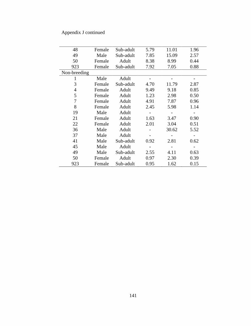
141

Appendix J continued

48 Female Sub-adult 5.79 11.01 1.96 49 Male Sub-adult 7.85 15.09 2.57 50 Female Adult 8.38 8.99 0.44 923 Female Sub-adult 7.92 7.05 0.88

Non-breeding 1 Male Adult - - - 3 Female Sub-adult 4.70 11.79 2.87 4 Female Adult 9.49 9.18 0.85 5 Female Adult 1.23 2.98 0.50 7 Female Adult 4.91 7.87 0.96 8 Female Adult 2.45 5.98 1.14 19 Male Adult - - - 21 Female Adult 1.63 3.47 0.90 22 Female Adult 2.01 3.04 0.51 36 Male Adult - 30.62 5.52 37 Male Adult - - - 41 Male Sub-adult 0.92 2.81 0.62 45 Male Adult - - - 49 Male Sub-adult 2.55 4.11 0.63 50 Female Adult 0.97 2.30 0.39 923 Female Sub-adult 0.95 1.62 0.15

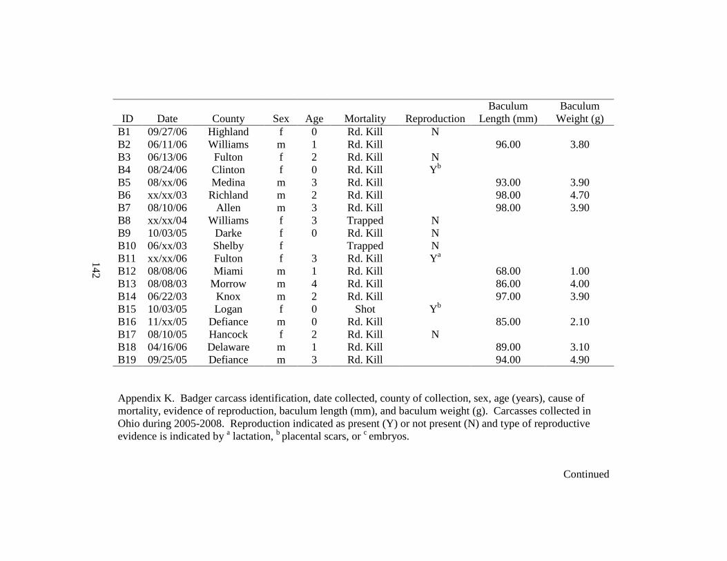
133

ID Date County Sex Age Mortality Reproduction Baculum

Length (mm) Baculum

Weight (g) B1 09/27/06 Highland f 0 Rd. Kill N B2 06/11/06 Williams m 1 Rd. Kill 96.00 3.80 B3 06/13/06 Fulton f 2 Rd. Kill N B4 08/24/06 Clinton f 0 Rd. Kill Yb B5 08/xx/06 Medina m 3 Rd. Kill 93.00 3.90 B6 xx/xx/03 Richland m 2 Rd. Kill 98.00 4.70 B7 08/10/06 Allen m 3 Rd. Kill 98.00 3.90 B8 xx/xx/04 Williams f 3 Trapped N B9 10/03/05 Darke f 0 Rd. Kill N B10 06/xx/03 Shelby f Trapped N B11 xx/xx/06 Fulton f 3 Rd. Kill Ya B12 08/08/06 Miami m 1 Rd. Kill 68.00 1.00 B13 08/08/03 Morrow m 4 Rd. Kill 86.00 4.00 B14 06/22/03 Knox m 2 Rd. Kill 97.00 3.90 B15 10/03/05 Logan f 0 Shot Yb B16 11/xx/05 Defiance m 0 Rd. Kill 85.00 2.10 B17 08/10/05 Hancock f 2 Rd. Kill N B18 04/16/06 Delaware m 1 Rd. Kill 89.00 3.10 B19 09/25/05 Defiance m 3 Rd. Kill 94.00 4.90 Appendix K. Badger carcass identification, date collected, county of collection, sex, age (years), cause of mortality, evidence of reproduction, baculum length (mm), and baculum weight (g). Carcasses collected in Ohio during 2005-2008. Reproduction indicated as present (Y) or not present (N) and type of reproductive evidence is indicated by a lactation, b placental scars, or c embryos. Continued

142

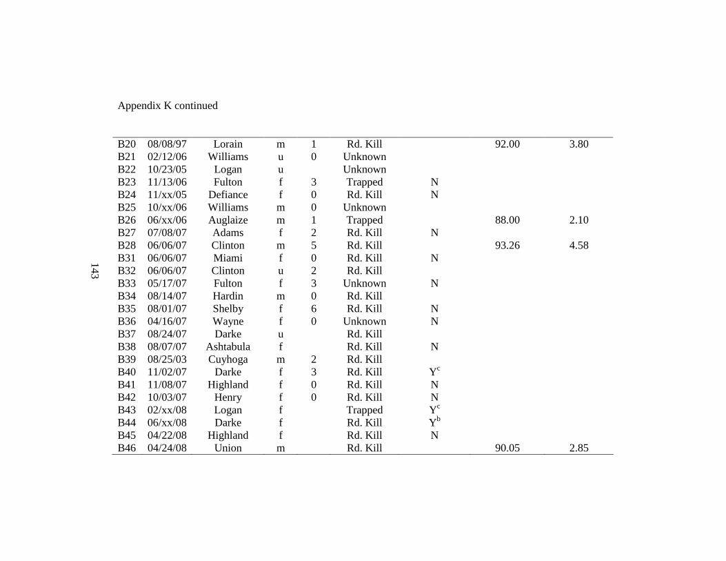
134

Appendix K continued B20 08/08/97 Lorain m 1 Rd. Kill 92.00 3.80 B21 02/12/06 Williams u 0 Unknown B22 10/23/05 Logan u Unknown B23 11/13/06 Fulton f 3 Trapped N B24 11/xx/05 Defiance f 0 Rd. Kill N B25 10/xx/06 Williams m 0 Unknown B26 06/xx/06 Auglaize m 1 Trapped 88.00 2.10 B27 07/08/07 Adams f 2 Rd. Kill N B28 06/06/07 Clinton m 5 Rd. Kill 93.26 4.58 B31 06/06/07 Miami f 0 Rd. Kill N B32 06/06/07 Clinton u 2 Rd. Kill B33 05/17/07 Fulton f 3 Unknown N B34 08/14/07 Hardin m 0 Rd. Kill B35 08/01/07 Shelby f 6 Rd. Kill N B36 04/16/07 Wayne f 0 Unknown N B37 08/24/07 Darke u Rd. Kill B38 08/07/07 Ashtabula f Rd. Kill N B39 08/25/03 Cuyhoga m 2 Rd. Kill B40 11/02/07 Darke f 3 Rd. Kill Yc B41 11/08/07 Highland f 0 Rd. Kill N B42 10/03/07 Henry f 0 Rd. Kill N B43 02/xx/08 Logan f Trapped Yc B44 06/xx/08 Darke f Rd. Kill Yb B45 04/22/08 Highland f Rd. Kill N B46 04/24/08 Union m Rd. Kill 90.05 2.85

143

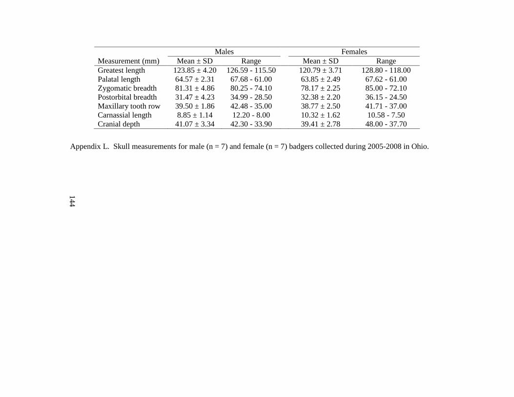
133

Appendix L. Skull measurements for male (n = 7) and female (n = 7) badgers collected during 2005-2008 in Ohio.

Males Females Measurement (mm) Mean ± SD Range Mean ± SD Range Greatest length 123.85 ± 4.20 126.59 - 115.50 120.79 ± 3.71 128.80 - 118.00 Palatal length 64.57 ± 2.31 67.68 - 61.00 63.85 ± 2.49 67.62 - 61.00 Zygomatic breadth 81.31 ± 4.86 80.25 - 74.10 78.17 ± 2.25 85.00 - 72.10 Postorbital breadth 31.47 ± 4.23 34.99 - 28.50 32.38 ± 2.20 36.15 - 24.50 Maxillary tooth row 39.50 ± 1.86 42.48 - 35.00 38.77 ± 2.50 41.71 - 37.00 Carnassial length 8.85 ± 1.14 12.20 - 8.00 10.32 ± 1.62 10.58 - 7.50 Cranial depth 41.07 ± 3.34 42.30 - 33.90 39.41 ± 2.78 48.00 - 37.70

144