Embed Size (px)
Citation preview
POPULATION AND LIVING STANDARDS IN ENGLAND
DURING ‘THE LITTLE ICE AGE’ 1
Cormac Ó Gráda
University College Dublin
Dublin 4
1 This paper borrows freely from Kelly & Ó Gráda (2010a, 2010b, 2010c), Campbell & Ó
Gráda (2010), and from an ongoing collaboration with Morgan Kelly and Joel Mokyr.
The comments of Ann Carlos and Kevin O’Rourke on a first draft are gratefully
acknowledged.
1
POPULATION AND LIVING STANDARDS IN ENGLAND
2007-2010 have been banner years for the publication of new
monographs on the European economy before the Industrial Revolution. Works
by economic historians Gregory Clark (2007), Jan de Vries (2008), Jan Luiten
van Zanden (2009), Bob Allen (2009), Joel Mokyr (2010), and Gunnar Persson
(2010) have greatly enriched the debate about the origins of modern economic
growth. All are written with a multidisciplinary readership in mind. Informed
by economic theory, they are also history-rich, employing new data on aspects
ranging from book publishing to human heights, and from patents to leisure.
They are also based on sophisticated understandings of the constraints imposed
by technology, and of the institutional and cultural contexts involved.
These interpretations of the origins of economic growth will undoubtedly
prompt neo-malthusian and post-malthusian growth theorists to further revise
and sharpen their models. This paper’s modest contribution to the debate is
empirical. It offers some new ‘facts’ on the English economy before the
Industrial Revolution and raises some questions about received ‘facts’.
1. ‘MALTHUSIAN’ CHECKS:
How common were serious harvest shortfalls in Europe in the past? How
often did they lead to subsistence crises or outright famine? One of the
important implications of Wrigley and Schofield’s classic reconstruction of
English population is that England’s demographic regime was ‘low pressure’ in
2
the pre-industrial era, in the sense that the short-run response to food price or
real wage shocks was modest. This echoes Malthus’s own belief that Europe
had long been less subject to the ‘ultimate check’ of death from famine than
the rest of the globe, and that while untold millions of European lives had been
blighted by malnutrition, ‘perhaps in some states an absolute famine may
never have been known’ (Malthus 1826: II, ch 13). Robert Fogel (2004)
similarly doubts the historical importance of famine. While emphasizing the
significance of hunger, he believes that scarcities arose more from
distributional inefficiencies than from genuine food availability declines. Less
sanguine and more critical assessments of the resilience of European
agriculture to exogenous environmental shocks in the pre-industrial era have
been offered by Karl-Gunnar Persson (1999: 47-64) and Rafael Barquin (2005).
One must beware of overgeneralization. Demographic data for medieval
England are scarce and hard to interpret, but they seem to offer evidence of a
demographic regime quite different to that of later centuries. Estimates of
mortality in medieval southern and central England have been derived from
manorial data. M. M. Postan and Jan Titow (1959) inferred a death rate
ranging from 40 to 52 per thousand for adult property-holders from heriot data,
while Zvi Razi’s estimates (1980) suggesting an adult life span of ‘between 18
and 22.8 years’ were based on court rolls. The resulting implied life
expectancies are implausibly low. More convincing recent evidence suggests
that landless males or monks who had managed to survive to age 20 in
medieval or late medieval southern England might have expected to live
3
another 27 years or so. However, even these numbers are still appallingly low
(Ecclestone 1999: 24; Hatcher et al. 2006; Wrigley et al. 1997: 290-91).
Ongoing research by Morgan Kelly and myself (Kelly & Ó Gráda 2010a)
confirms the vulnerability of medieval Englishmen and Englishwomen to harvest
shortfalls. Following Ronald Lee (1981) and others we measure the short-run
response of mortality to adverse price and wage shocks. Continuous data on
deaths are lacking, so we rely on proxies stemming from the feudal system.
Here I describe one proxy consisting of over twelve thousand entry fines paid
by tenants on the Winchester estates in southern England in order to inherit
land between the 1260s and the Black Death in 1349.2 By counting the annual
number of these transfers listed as inheritances, we can see how strongly
deaths responded to harvest yields and earlier mortality. The number of
inheritances shows two spikes where we would expect them: in 1317 at the
peak of the Great Famine, and in 1349, the first year of the Black Death.
The social status of those who died may be inferred from the size of the
entry fine their heirs paid. To be a middling farmer required about a half-
virgate (roughly 20 acres usually) of land, which commanded in the early
fourteenth century an entry fine of at least 30 to 40 shillings, and often
considerably more. This corresponds to the largest 10 to 15 per cent of fines in
our sample, the median fine in our post-1302 sample being 7.5 shillings. Typical
estimates for the early fourteenth century are that about half of all tenants
owned less than a quarter virgate, the bare minimum for subsistence (Titow
2 These data were compiled by Mark Page (2006).
4
1969: 78–81). In other words, then, most of the tenants in our sample of fines
are semi-proletarian smallholders with too little land to support themselves.
Manors varied considerably in size and continuity of records. For the period
before 1349, the ten largest manors accounted for fifty per cent of deaths, and
the largest twenty for seventy per cent, and these large manors have almost
continuous records. By contrast, records for the smallest manors are extremely
fragmentary.
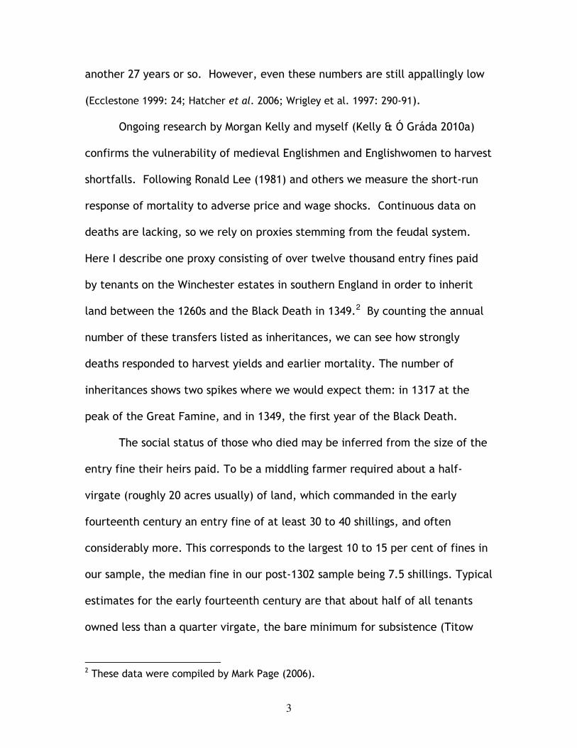
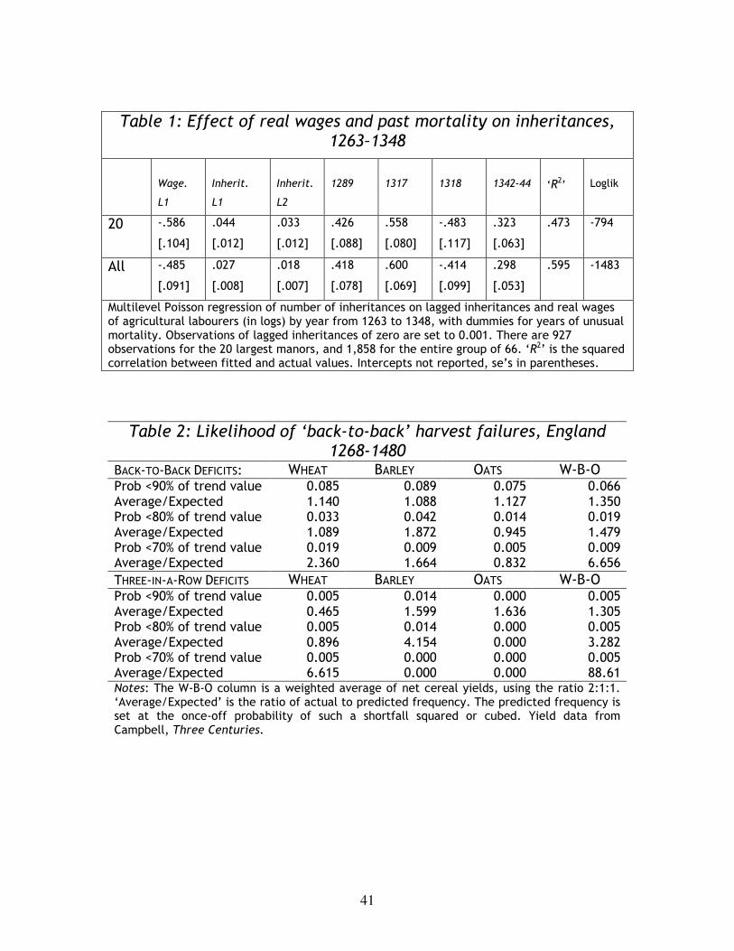
Annual fluctuations in fines were highly sensitive to cereal prices and
real wages. Table 1 reports the results of a regression of number of
inheritances on each manor on the real wages and inheritances on the same
manor in the two previous years; both for the twenty largest manors and the
entire sample. Dummies are added for years of unusual mortality: 1269, 1317,
1318 and 1342–44. Mortality responds strongly to real wages in the previous
year, with an elasticity exceeding one half. Note too that increased mortality
in one year is followed by slightly higher mortality in the two following years.
This slight positive autocorrelation is in contrast to the strong negative
autocorrelation in mortality after the sixteenth century. The size distribution
of fines allows us also to see if years of severe epidemic mortality—1317 and
1349— had different social distributions of mortality than ordinary years. After
1303, the median fine is 80 pence, identical to the median fines in 1317 and
1349, suggesting that tenants at all levels suffered equally during these crises.3
3 This assumes, however, that fines were ‘sticky’ in bad years.
5
[Table 1 about here]
The English nobility were legally tenants of the king which meant that
when a noble died without adult children, their estates reverted to the crown.
To determine the value of the property and the existence of possible heirs, an
Inquisitio Post Mortem (IPM) was carried out, usually by neighbouring nobles.
The records of all surviving IPMs from 1300 to the Black Death were used by
Campbell (2005) to assess the income of the English nobility, and these data
can be used as a proxy for annual male deaths among that class. An analysis of
the relationship between real wages in one year and IPMs in the next produces
similar results to those reported in Table 1, implying that wealth was no shield
against death from epidemic disease that had incubated among hungry
peasants: the elasticity of mortality with respect to the real wage of
agricultural labourers was almost as high as in Table 1 (Kelly & Ó Gráda 2010a).
In the medieval era we find that falls in real wages caused by poor wheat
harvests were deadly at all levels of society.
Newly available micro-level crop yield data endorse the view that in
England, as in most of Europe, at least until at 1500AD, and probably for far
longer, major food availability declines underpinned many if not necessarily all
episodes of pronounced grain-price inflation. Combining price and crop yield
data implies—contrary to Fogel’s claim in the Escape from Hunger (2004)—that
pre-industrial European price elasticities of demand for grain were not low and
6
are likely to have been significantly higher in the medieval and early modern
periods than in the late nineteenth century when official agricultural statistics
first become available (Campbell and Ó Gráda 2010).
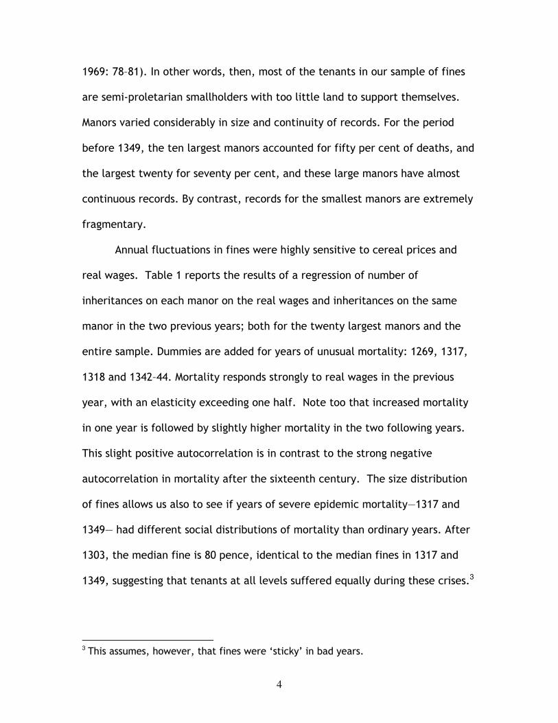
Between the mid-13th and late-15th centuries crop shortfalls of more
than one-fifth were not unusual and in the worst harvests of all shortfalls of
more than two-fifths are recorded. The most dangerous situations, however,
were those which resulted from back-to-back harvest failures of all the major
crops, and these were far less frequent, occurring perhaps once a generation or
less (compare Ó Gráda 2007). Harvest failures on the scale of 1315-17 or 1349-
51 were once in 200-year events, hence the occurrence of two such harvest
disasters within the narrow space of a single generation prompts speculation as
to whether there was an element of autocorrelation in the precipitating
environmental causes.
[Table 2 about here]
2. MEDIEVAL TO EARLY MODERN
The belief that there was no sustained improvement in living standards
before the Industrial Revolution informs modern unified growth theory. In
Oded Galor’s words, the pre-industrial world was ‘in a low level equilibrium in
terms of income per capita… The growth of total output resulting from
7
technological progress [was] matched by population growth so that per capita
income fluctuate[d] around a low stable level, with no significant progress in
average living standards over a long period of time.’ Or, to quote Robert Lucas
(1996), ‘Three hundred years ago, living standards in all economies in the world
were more or less equal to one another and more or less constant over time’.
Clark in Farewell to Alms claims likewise.
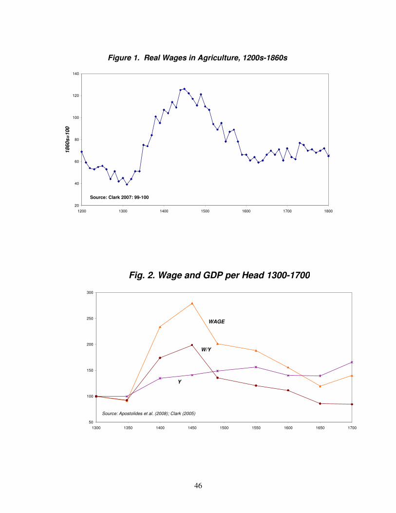
Recently-constructed time series by Allen and Clark describe a dramatic
fall in real wages in England between the late fifteenth and the early
seventeenth centuries, with stasis or mild recovery thereafter. Figure 1
summarizes Clark’s findings: fluctuations but no sustained increase before the
Industrial Revolution.
How does this square with the shift from the harsh medieval
demographic regime just described to one in the seventeenth century showing
but the faintest evidence of a link between low wages and high mortality
(Nicolini 2007; Kelly and Ó Gráda 2010a)? Did living standards really fail to rise?
Surely the shift in demographic regimes suggests that something must have
changed between the Middle Ages and the two centuries of so before the
Industrial Revolution? In what follows I present some evidence in favour of a
rise in living standards over this period which fits with the described above.
[Figure 1 about here]
2.1. Life expectancy
8
Above I reported estimates of e(20) of about 27 years for medieval
England. In the seventeenth century, however, Englishmen and Englishwomen
who survived to age 25 had on average another 31 years to live; in the
eighteenth century, another 34 years.4 Such increases in life expectancy can
only have added to the ‘true’ standard of living. In the model first proposed by
Dan Usher (1973) and applied by Jeffrey Williamson to England during the
Industrial Revolution (Williamson 1984: 158-60; compare Becker, Philipson, &
Soares 2005), the rise in the ‘true’ standard of living would depend on the
proportionate increase in life expectancy and the assumed elasticity of annual
utility to annual consumption. For example, assuming an elasticity of 0.5 and
an increase in e(0) of one-tenth5 would have meant a gain of one-fifth in ‘true’
living standards. Moreover, increasing life expectancy is not just a component
of the current standard of living; it also prompts increases in future living
standards.6
Demographic regimes in England and France also diverged, with death
rates in pre-revolutionary France much higher on average. In the first half of
the eighteenth century e(0) in England was about 35-37 years; in mid-
eighteenth century France e(0) was about 25 years. French mortality also
4 In Malthusian equilibrium such increases would have required either a reduction in
the subsistence wage or a compensating movement in how births responded to wages.
5 Since gains to the life expectancy of young adults would not affect the significant
proportion dead before age 20 or 25.
6 See e.g. Aghion et al. 2009.
9
varied more, although fluctuations in both counties show signs of attenuation
over time. Between 1670 and 1720 France was subject to three major crises
while England was virtually immune; thereafter vital rates fluctuated less in
both countries, with the important exceptions of 1727-30 and, to a lesser
extent, 1740-42 in England.
2.2 GDP and Wages
According to Clark (2009: 1160), Angus Maddison’s widely-used historical
GDP data ‘have an imprimatur that is completely out of line with their dubious
provenance’. Be that as it may, the more careful, if still tentative, estimates
of Apostolides et al. (2009a) deserve serious consideration, and they tell a
story very different to that told by real wage series (Figure 2). They imply that
between 1450 and 1700 GDP per head rose by one-sixth; over the same period,
Clark’s real wages dropped by half.7
This is a reminder of a dimension marginalized in Clark’s account: the
distribution of income. Granting, just for the sake of argument, the claim that
medieval English agricultural labourers were no better off than foragers and
cavemen, the comparison overlooks the likely reduction in the share of such
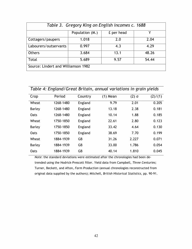
unskilled labourers in total employment after the Middle Ages. By Gregory
King’s reckoning cottagers, paupers, labourers, and servants together
7 It also bears noting that several of the studies of GDP per head elsewhere in Europe
in this period presented at the IEHA Utrecht meetings in August 2009 record mild
increases or, at worst, modest declines. These papers are still available online at:
http://www.wehc2009.org/programme.asp.
10
represented only one-third of the population in 1688 and received only one-
ninth of income (Table 3). The remaining two-thirds received an average of
over four times as much.
[Table 3 and Figure 2 about here]
2.3. Output and Price Variability
Campbell and Ó Gráda (2010) argue that grain harvests in England were
both substantially heavier and significantly less variable in the eighteenth
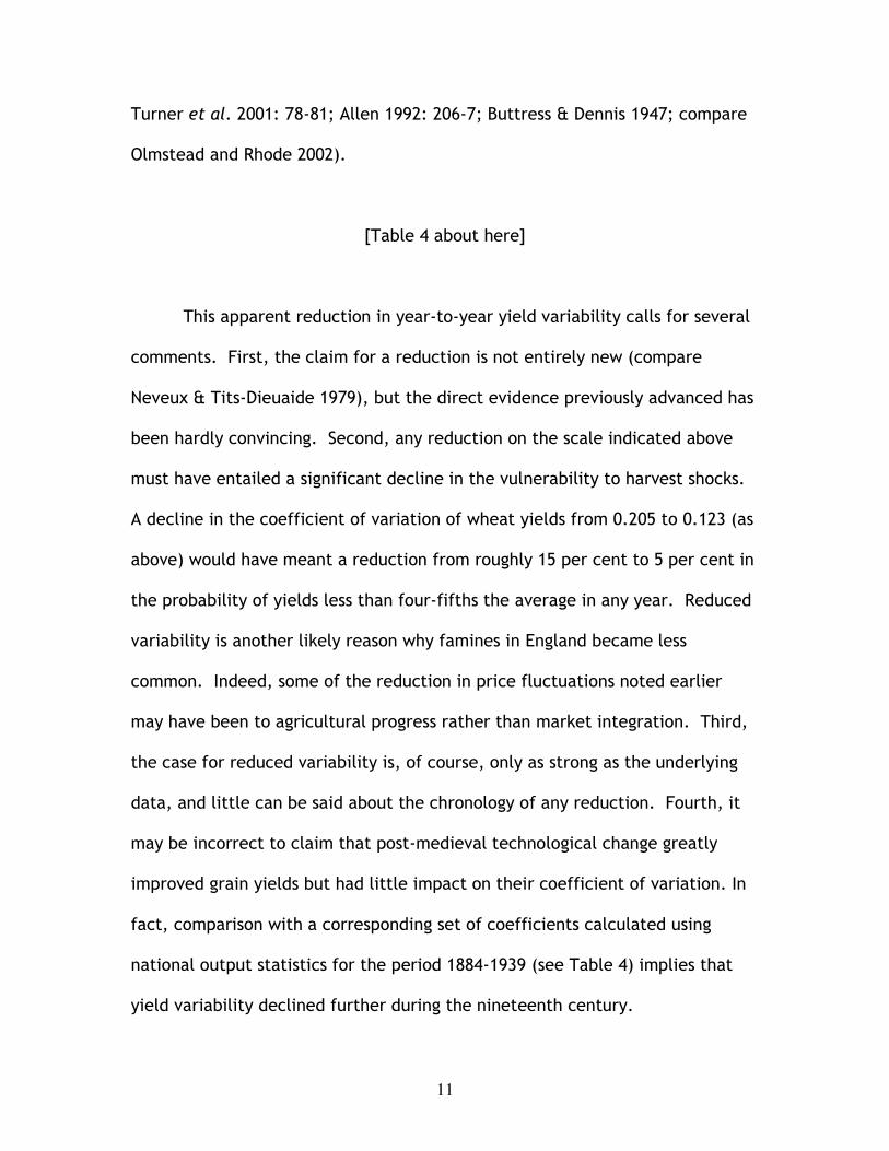
century than in the fourteenth or fifteenth. Table 4 compares the coefficients
of variation calculated on de-trended annual chronologies of gross yields of
wheat, barley, and oats for the periods 1268-1480 and 1750-1850. The
coefficients of variation for wheat and barley are a quarter to a third lower by
1750-1850: only the variability of oats yields showed no improvement.
Precisely how this was achieved remains to be established but a likely
explanation is the biological innovation of selecting and sowing sounder seed.
The range of solutions to crop damage caused by rain, fungi, weeds, and pests
proposed in print grew from the sixteenth century onwards, and while evidence
for a specialist seed trade is lacking for medieval England, there is increasing
evidence for it from the seventeenth century onwards. None of this proves the
efficacy of specific ‘remedies’ but points to the ubiquity of processes of
experimentation, adaptation, and learning-by-doing that sought to minimize
the risk of poor harvests, and so improve the standard of living (Thick 1990;
11
Turner et al. 2001: 78-81; Allen 1992: 206-7; Buttress & Dennis 1947; compare
Olmstead and Rhode 2002).
[Table 4 about here]
This apparent reduction in year-to-year yield variability calls for several
comments. First, the claim for a reduction is not entirely new (compare
Neveux & Tits-Dieuaide 1979), but the direct evidence previously advanced has
been hardly convincing. Second, any reduction on the scale indicated above
must have entailed a significant decline in the vulnerability to harvest shocks.
A decline in the coefficient of variation of wheat yields from 0.205 to 0.123 (as
above) would have meant a reduction from roughly 15 per cent to 5 per cent in
the probability of yields less than four-fifths the average in any year. Reduced
variability is another likely reason why famines in England became less
common. Indeed, some of the reduction in price fluctuations noted earlier
may have been to agricultural progress rather than market integration. Third,
the case for reduced variability is, of course, only as strong as the underlying
data, and little can be said about the chronology of any reduction. Fourth, it
may be incorrect to claim that post-medieval technological change greatly
improved grain yields but had little impact on their coefficient of variation. In
fact, comparison with a corresponding set of coefficients calculated using
national output statistics for the period 1884-1939 (see Table 4) implies that
yield variability declined further during the nineteenth century.
12
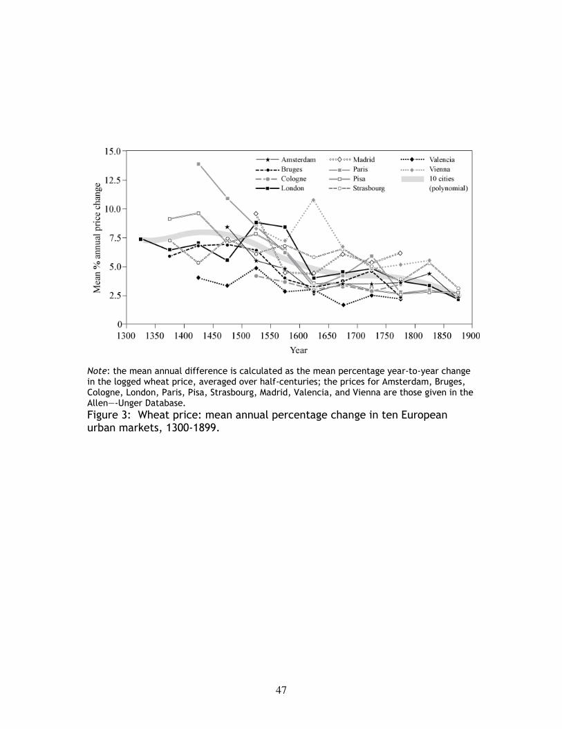
In the past several scholars (e.g. Persson 1999; Rönnbäck 2009) have
highlighted the role of increasing market integration in the early modern era
(compare Figures 3 and 4). In similar vein McCloskey and Nash (1984) have
pointed to the reduction in the cost of storage and increased intertemporal
arbitrage due to reduced interest rates. Without wanting to dismiss such
improvements, I would also include the role of reduced crop yield variability in
reducing price fluctuations.
In sum, the vulnerability to famine that characterized the Middle Ages
had been already largely banished by the time Malthus wrote his Essay. This
signal achievement contributed materially to the wellbeing of the humblest
members of society. It probably owed little to any exogenous change in
environmental hazards (on which more below) and a lot to the improved
capacity of governments, farmers, markets, and society at large to cope with
shocks.
[Figures 3 and 4 about here]
2.4. Welfare
Morgan Kelly and I (2010c) argue that the nation-wide system of public
poor relief put in place in England in the late sixteenth century—known as the
Old Poor Law—better protected the food entitlements of the most vulnerable in
hard times, and thereby limited both life-cycle and harvest-induced destitution.
The poor law squared a concern for economy with effective relief. The system
13
had its limits; it could not prevent excess mortality from famine in the late
1720s and early 1740s. However, those crises were minor relative to earlier. We
argue that the institutional form of the Old Poor Law owed as much to English
history as it did to increasing income. Nonetheless, elites had a long-standing
interest in limiting the spread of infectious disease and the anti-social
behaviour that accompanied subsistence crises, and the rise in GDP per head
after 1500 enabled them to act.
2.5. Further considerations
De Vries (2008) highlights the role of increasing variety and colonial
goods in the ‘industrious revolution’. Jonathan Hersh & Hans-Joachim Voth
(2009) go further, calculating the welfare gain to Britain of three ‘new goods’,
tea, coffee, and sugar. Employing various measures of this gain, the simplest
of which is that proposed by Hausman (1999), they reckon the welfare gain
from their ‘new goods’ at about one-sixth of consumer expenditure by the
eighteenth century.
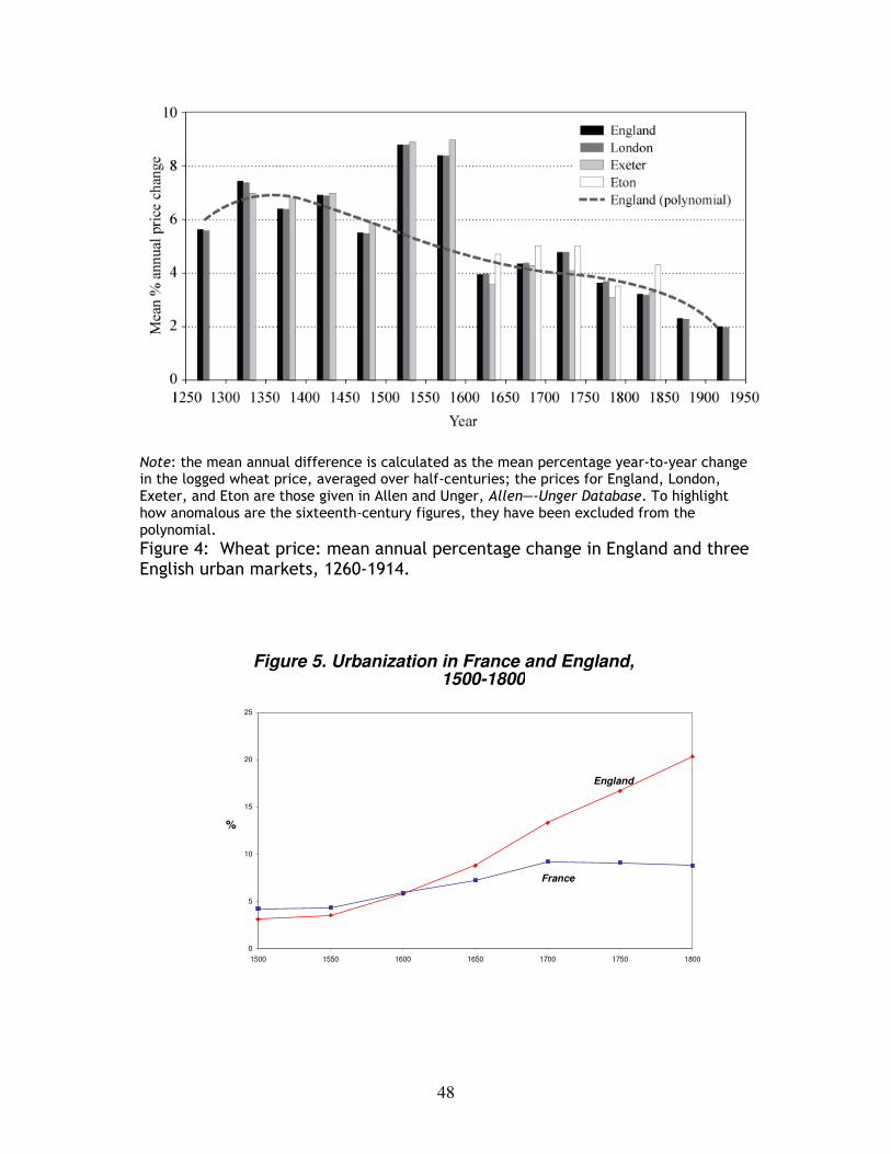
The urbanization ratio is an imperfect measure of the share of the
labour force in non-agricultural occupations (Persson 1992). Nonetheless, the
huge rise in the proportion of city- and town-dwellers in England from 1500 on
(see Figure 5, based on de Vries 1984: 39) implies productivity growth in
agriculture, particularly since England was a food-exporting economy at the
end of the period. Again, an increase in average living standards is indicated,
14
although this must be weighed against the demographic penalty associated with
urbanization (Wrigley 1985).
Finally, there was also a huge increase in literacy over the same period.
In England the proportion of grooms who could sign the marriage register—a
commonly accepted measure of literacy—rose from only 6 percent in 1500 to
over three-fifths in 1750, and was already significant by 1650 (Allen 2009: 12;
Houston 1982). The increased ability to afford the investment in schooling and
acquiring literacy also points to rising living standards. The link in cross-
section in a later era between literacy, on the one hand, and measures of
health and well-being such as housing quality and mean adult height, on the
other, certainly point in that direction.
[Figure 5 about here]
In sum, a range of considerations rejects the impression of no sustained
improvement in living standards before the Industrial Revolution. This
suggests that while real wage series may usefully reflect the lot of those at the
very bottom of the socio-economic ladder, they are a fallible indicator of long-
run trends in living standards more broadly defined.
15
3. WEATHER MATTERED, CLIMATE DIDN’T
Our context so far has been a Malthusian world in which demographic
adjustment eventually whittles away any rises—or falls—in real incomes. But
living standards could also have been held back by non-Malthusian forces.
Several non-Malthusian scholars have linked economic hardship in the medieval
and early modern eras to climate change (e.g. Campbell 2010; Steckel 2004).
Meteorologist Hubert Lamb, the first to draw the link between a Little Ice Age
and broader economic and social trends, has drawn attention to the alleged
‘parallelism of climatic and cultural curves’ (1995: 318) as the Little Ice Age
drew to a close. Richard Steckel has blamed the Little Ice Age for a cooling
trend that ‘wreaked havoc’ on northern Europe for half a millennium, while
Brian Fagan has recently described it as a defining period that ‘changed the
course of European history... changed European agriculture, helped tip the
balance of political power from the Mediterranean states to the north, and
contributed to the social unrest that culminated in the French Revolution’.
Against such claims, Emmanuel Le Roy Ladurie and others have argued that the
economic and (by implication) political impact of the Little Ice Age was
insignificant (Lamb 1995: 318; Steckel 2004; Fagan 2000; Le Roy Ladurie 1971).
A combination of resonant images has linked the Little Ice Age firmly to
Northern and Western Europe. These images include the collapse of
Greenland’s Viking colony and the demise of grape-growing in southern England
in the late medieval era; the Dutch winter landscape paintings of Bruegel the
Elder (1525-69) and Avercamp (1585-1634); the periodic ‘ice fairs’ on London’s
16
Thames, ending in 1814; and, as the Little Ice Age waned, the contraction of
Europe’s Nordic and Alpine glaciers.
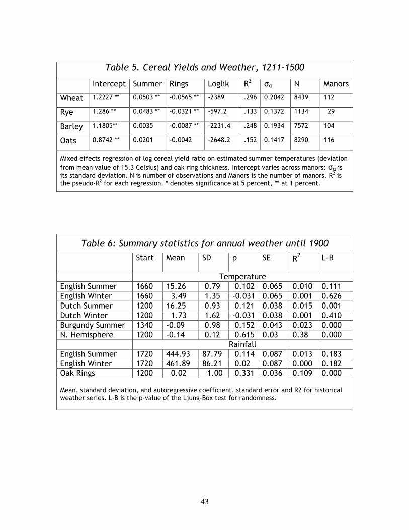
How much did this alleged cooling matter? On thing is evident: in
medieval Europe crop yields were very sensitive to weather. Combining
Campbell’s crop yield data with meteorological data described in more detail
below, Morgan Kelly and I (2010) find that a one degree rise in summer
temperature (equivalent to a change of 1.5 standard deviations) increased
average wheat yields by 5 per cent, while a one standard deviation increase in
the thickness of oak rings (a weather proxy, on which more below) is associated
with a fall of 5.6 per cent in average output. Other crops were less sensitive to
weather, and in the expected order. Rye produces coefficients of 0.05 and
−0.03 for temperature and tree rings; barley appears unaffected by summer
temperature, and has a coefficient of only −0.01 for tree rings; and oats show
no measurable effect of weather at all (Table 5). I terms of weather risk, oats
offered the best insurance, and had the added advantages of growing on poorer
soil than other grain, and producing more calories per acre. Consequently,
while weather strongly affected wheat yields, it does not appear to have had a
large impact on the spring grains, such as oats, on which ordinary people
relied. Oats offered the best insurance against bad weather, besides having
the added advantages of growing on poorer soil than other grain, and producing
more calories per acre.
[Table 5 about here]
17
These estimates convey a sense of the damage a significant cooling in
temperatures might have inflicted on agriculture in early modern Europe.
Assuming linearity, a reduction of two degrees in summer temperatures—
significant even by twentieth-first century standards—would have cut wheat
yields by one-tenth.8
Originally applied in 1939 to an era spanning several millennia in
California’s Sierra Nevada, the term ‘Little Ice Age’ now usually refers instead
to a global climatic shift towards colder weather occurring during the second
millennium. Considerable imprecision about the chronology, geography, and
impact of the Little Ice Age remains, however. The chronology of the
preceding Medieval Warm Period, identified by Lamb in 1965, is equally elastic.
Consensus has also been lacking on the Little Ice Age’s geographical reach.
The Intergovernmental Panel on Climate Change’s Third Assessment Report
emphasizes the variations in climate change across regions and the possible
independence of such variations, so much so that it deems the term ‘Little Ice
Age’ a misleading guide to global temperature changes in the past. True, in
the Northern Hemisphere the 1500-1900 period stands out, although
temperature change even then appears to have been modest relative to that
experienced in the twentieth. More recent assessments of the Medieval Warm
8 However, to the extent that agents would have adapted to the challenge by altering
crop mixes, this is an upper-bound estimate of the likely cost.
18
Period also reckon it to have been only moderately milder than the cooling
period that followed.
The ambiguities arise in part from the lack of direct measurements of
temperature before the introduction of reliable thermometers in the mid-
seventeenth century. Lacking long-run time series data, early accounts of the
Little Ice Age (such as Lamb 1965) relied on impressionistic and anecdotal
evidence. Uncertainty is compounded by the somewhat conflicting patterns
revealed by the now numerous proxy measures of climate change.
Geologist François Matthes (1939) linked his original ‘Little Ice Age’ to
the growth of Sierra Nevadan glaciers following a mid-Holocene thermal
maximum, and this prompted others to reconstruct historical glacier lengths
(e.g. D'Orefice et al. 2000; Oerlemans 2001). Glacial retreat since the late
nineteenth century has become one of the hallmark images of global warming.
Tree rings offer a second measure of secular climate change: warm and wet
weather are associated with faster growth and wider rings (Baillie 1999). Le
Roy Ladurie was the first to propose changes in the timing of the grape harvest
as a measure of long-run climate change. His analysis of the starting dates of
pinot noir harvests in Burgundy, as updated by Isabelle Chuine and her co-
authors, reports April—August temperature anomalies with reference to the
1960-1989 period for the city of Dijon (Le Roy Ladurie 1971; Chuine et al.
2004).
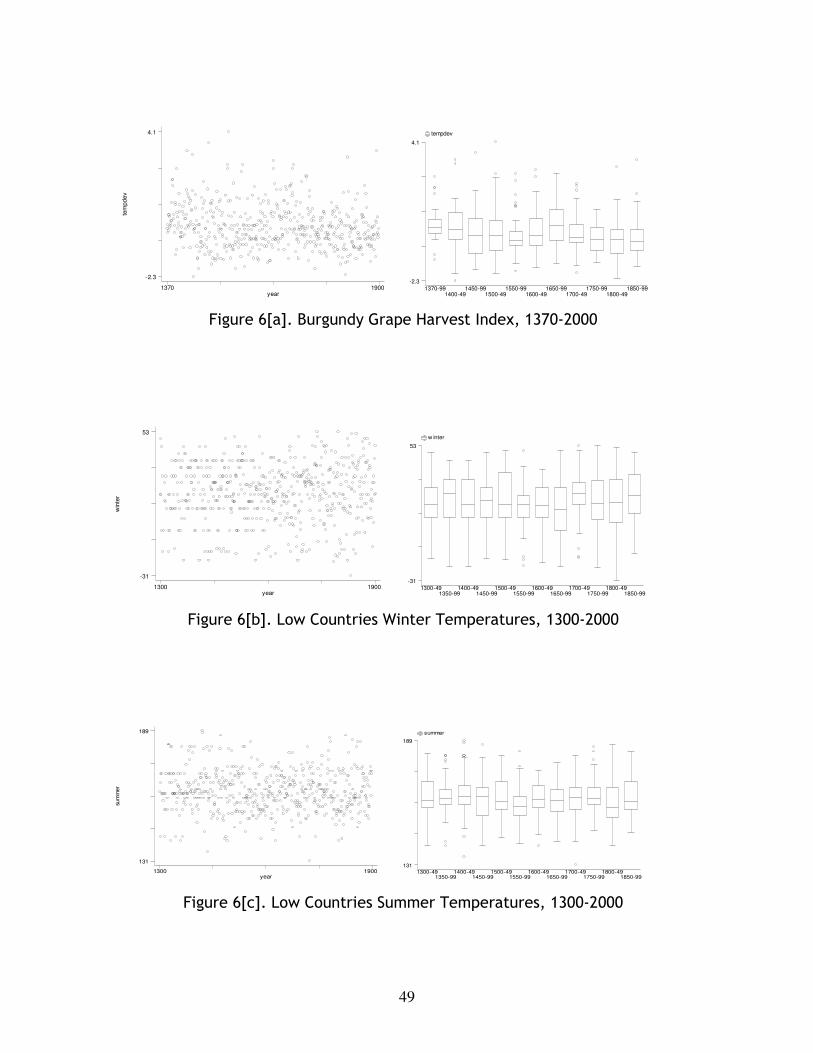
Time series derived from Northern Hemisphere ice cores—ice cylinders
drilled out of polar ice sheets and mountain glaciers—offer another measure of
19
long-term climate change. Yet another valuable source is winter and summer
temperature series for the Low Countries that rely on documentary data
ranging from letters and diaries to toll accounts to produce weather indices
rated on a scale from 1 (=extremely cold) to 9 (=extremely hot). The series
yield only scattered data before 1300, but are continuous, or almost so,
thereafter (van Engelen et al. 2001). The reconstructions present their own
different stories. For example, the most northerly ice cores imply much more
volatile weather than more southerly ice cores and other reconstructions.
[Table 6 and Figure 6 about here]
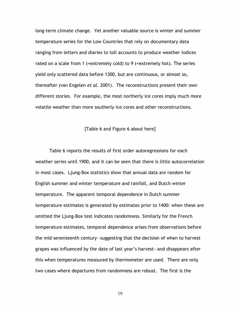
Table 6 reports the results of first order autoregressions for each
weather series until 1900, and it can be seen that there is little autocorrelation
in most cases. Ljung-Box statistics show that annual data are random for
English summer and winter temperature and rainfall, and Dutch winter
temperature. The apparent temporal dependence in Dutch summer
temperature estimates is generated by estimates prior to 1400: when these are
omitted the Ljung-Box test indicates randomness. Similarly for the French
temperature estimates, temporal dependence arises from observations before
the mid-seventeenth century—suggesting that the decision of when to harvest
grapes was influenced by the date of last year’s harvest—and disappears after
this when temperatures measured by thermometer are used. There are only
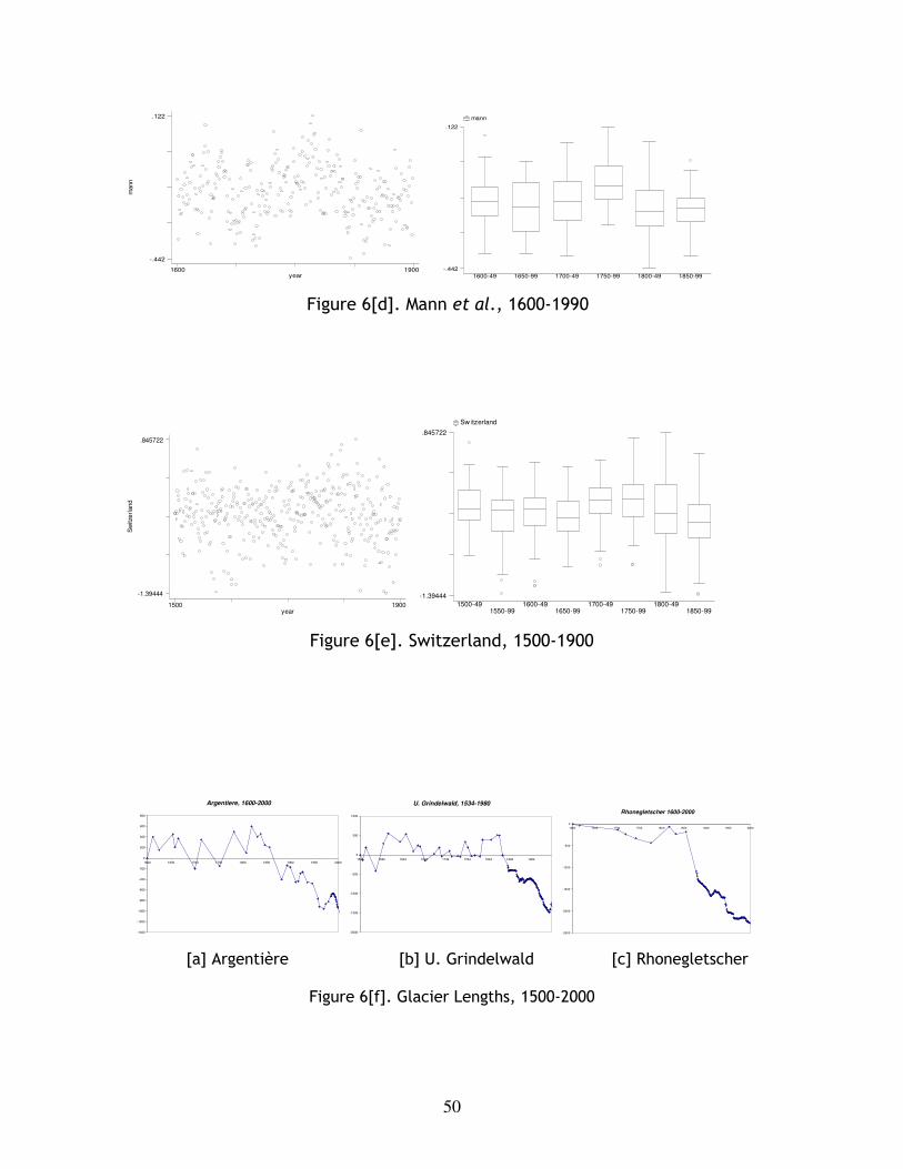
two cases where departures from randomness are robust. The first is the
20
Mann, Bradley & Hughes (1999) Northern Hemisphere temperature series
which, we have seen, had no explanatory power for cereal yields, and appears
to be driven by variations in conditions at high latitudes where there is
evidence of long swings in climate (Dawson et al., 2007). The second is the oak
ring series which reflects the fact that oak tree are large, slow growing
organisms (using innovations in oak ring thickness rather than actual thickness
gave substantially identical results in predicting cereal yields). The estimated
power spectra of all series except Northern Hemisphere temperature were
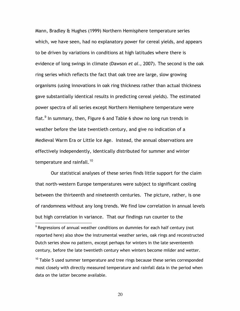
flat.9 In summary, then, Figure 6 and Table 6 show no long run trends in
weather before the late twentieth century, and give no indication of a
Medieval Warm Era or Little Ice Age. Instead, the annual observations are
effectively independently, identically distributed for summer and winter
temperature and rainfall.10
Our statistical analyses of these series finds little support for the claim
that north-western Europe temperatures were subject to significant cooling
between the thirteenth and nineteenth centuries. The picture, rather, is one
of randomness without any long trends. We find low correlation in annual levels
but high correlation in variance. That our findings run counter to the 9 Regressions of annual weather conditions on dummies for each half century (not
reported here) also show the instrumental weather series, oak rings and reconstructed
Dutch series show no pattern, except perhaps for winters in the late seventeenth
century, before the late twentieth century when winters become milder and wetter.
10 Table 5 used summer temperature and tree rings because these series corresponded
most closely with directly measured temperature and rainfall data in the period when
data on the latter become available.
21
conventional wisdom on the Little Ice Age reflects our statistical approach. We
analyse unsmoothed annual data, whereas the current practice in climatology
is to smooth data using a moving average or other filter prior to analysis. When
data are uncorrelated, as European weather series appear to be, smoothing can
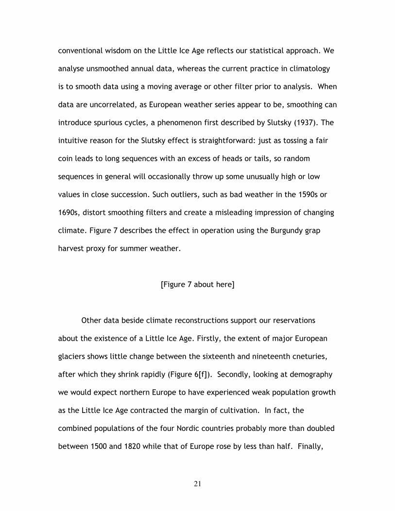
introduce spurious cycles, a phenomenon first described by Slutsky (1937). The
intuitive reason for the Slutsky effect is straightforward: just as tossing a fair
coin leads to long sequences with an excess of heads or tails, so random
sequences in general will occasionally throw up some unusually high or low
values in close succession. Such outliers, such as bad weather in the 1590s or
1690s, distort smoothing filters and create a misleading impression of changing
climate. Figure 7 describes the effect in operation using the Burgundy grap
harvest proxy for summer weather.
[Figure 7 about here]
Other data beside climate reconstructions support our reservations
about the existence of a Little Ice Age. Firstly, the extent of major European
glaciers shows little change between the sixteenth and nineteenth cneturies,
after which they shrink rapidly (Figure 6[f]). Secondly, looking at demography
we would expect northern Europe to have experienced weak population growth
as the Little Ice Age contracted the margin of cultivation. In fact, the
combined populations of the four Nordic countries probably more than doubled
between 1500 and 1820 while that of Europe rose by less than half. Finally,
22
focusing more narrowly on England, between 1450 and 1700 English agriculture
saw neither the decline in the share of wheat in tillage acreage nor the relative
decline in wheat yields that one might have expected.
Lamb and Fagan devoted considerable ingenuity to explaining many
trends and events in European history through climate change. The task now is
to seek complementary and alternative explanations for such trends and
events. In the case of the collapse of Greenland’s Nordic colony, for example,
recent scholarship has de-emphasized the role of climate. Alternative
potential explanations have been proposed, including competition for resources
with the Inuit; the decline of Norwegian trade in the face of an increasingly
powerful German Hanseatic League; the increasing availability of African ivory
as a cheaper substitute for walrus ivory; the diversion of English fishing vessels
from Greenland to Labrador and Newfoundland in the fifteenth century;
overgrazing by livestock; bubonic plague; and marauding pirates (Roesdahl
1998; Seaver 2009). Moreover, the decline of wheat and rye cultivation in
Norway from the thirteenth century may owe more to lower German cereal
prices than any temperature change (Miskimin 1975: 59). Nor should too much
be made of the imagined landscapes of Bruegel or Avercamp. Although the
latter made a living from his lively if formulaic winter scenes, it must be said
that such landscapes rarely feature in the work of other better known Dutch
landscape artists such as Albert Cuyp or Jan van Goyen. Note too that
Bruegel’s much-reproduced ‘Hunters in the Snow’ (Lamb 1995: 233-34) was
23
painted in the wake of the coldest winter in the Low Countries between 1435
and 1684.11
The alleged virtual disappearance of grape cultivation in late medieval
England does not need a Little Ice Age either. England’s grape acreage during
the middle ages was miniscule: the forty-five vineyards recorded in the
Domesday Book (1086) were for the most part recently planted, small in size,
and catered mainly to the requirements of the Anglo-Norman nobility and to
the church. Total output is unlikely to have exceeded 3,500 litres12, implying a
per capita consumption of close to zero. Nor is quality likely to have matched
that of continental vineyards; indeed, some of the output was consumed as
verjuice (a flavor-enhancing liquid made from unripe white grape varieties)
rather than wine. Thus a more plausible explanation for the decline in English
wine production is reductions in transactions costs that permitted England to
pursue its comparative advantage. This is supported by the increasing
importance of wine imports from France from the twelfth century on, until
interrupted by the Hundred Years War (James 1951). It is also consistent with 11
Even so it is just one of a cycle of six paintings describing different seasons of the
year and none of the others hints at an LIA. Five survive, including the equally well-
known ‘The Harvesters’, held in New York’s Metropolitan Museum.
12 The only yield reported in Domesday refers to the vineyard at Rayleigh, Essex,
where six arpents yielded twenty modii in a good year (si bene procedit) (Darby 2007:
372). Assuming that the Domesday modius was the same as the Roman measure, this
would imply about 30 litres per arpent. If the average vineyard had 3 arpents (about
three acres) under grapes, then this implies a very rough aggregate estimate of 3,500
litres.
24
the much higher price of wine relative to beer in England: in the early
fourteenth century a gallon of wine cost about 5 to 7 times as much as a gallon
of ale in England, but in France the ratio was about one.13
In sum, we find no evidence for the case for climate change as an
explanation for economic trends in early modern Europe.
4. HIGH WAGES, DEAR LABOUR?
Real wage trends, as measured by Allen and Clark, fail to capture the
increase in living standards that must have taken place in England between the
Middle Ages and Industrial Revolution. Real wage data are a more reliable
guide to cross-sectional differences in living standards. But are they also a
reliable measure of productivity differences? Allen (2009) implicitly believes
they are, since he argues that in late eighteenth-century and early nineteenth-
century England high wages, by inducing the necessary labour-saving
technological changes or endogenous innovation, drove the Industrial
Revolution. The hypothesis—echoing Habakkuk (1962) on Anglo-American
comparisons—consists of two claims. The first is that real wages were high in
England relative to elsewhere. The second is about the link between wages
and induced labour-saving technical change. Our concern in this final section
of the paper is with the first hypothesis.
13 Compare Dyer 1989: 58, 62; Unger 2004: 74-77.
25
Data produced by Allen are consistent with Arthur Young’s claim in the
wake of his French travels in 1787-89 that in the agricultural sector nominal
wages in England were almost double those in France (£33.5 versus £19).
Deflating these wages by the respective prices of bread would erode much of
the difference, Young conceded, but would not be legitimate because ‘in
England the rate of labour, supposing it to depend on provisions, would
certainly depend, not on bread only, but on an aggregate of bread, cheese, and
meat’ (Young 1793: II, 315-16). Despite this, Young was not convinced that
French labour was proportionately cheaper than English, because ‘strength
depends on nourishment; and if this difference be admitted, an English
workman ought to be able to do half as much work again as a Frenchman’. So
were wages in Britain really that ‘high’?
4.1. Heights and wages
Young did not pursue the issue further, but data on adult heights in
England and France c. 1800 support his assertion that British workers were
physically stronger than French. Figure 8 describes the average heights of
French army recruits and English male convicts (Weir 1997: 191; Nicholas &
Steckel 1991). Both sets of data refer to cohorts born between 1780 and 1815.
I have added 1 cm. to the French heights to reflect the fact that they refer to
recruits who had not yet reached full adult height.14 The comparison suggests
that the gap between French and English heights on the eve of the Industrial
14
They were aged 20-21 years.
26
Revolution was considerable—about four centimetres. Moreover, if socially
more representative data for England were available (i.e. not just transported
convicts, who came disproportionately from poor backgrounds), the likelihood
is that the gap would be wider still (compare Fogel 2004: 13).
[Figure 8 about here]
The significant height advantage of British workers meant that they were
physically stronger and more productive than their French counterparts.
Current physiological research documents the link between height and grip or
muscle strength.15 But how much did height matter for productivity? There is
no direct answer, but the development economics literature provides ample
evidence that taller workers earn higher wages. Individual heights are partly
genetically determined, and partly the product of human capital, education
and net nutrition in childhood and adolescence. In a series of studies based on
modern African and Brazilian individual-level data, Schultz (2002, 2005) finds
15 For example, a recent study of Indian female labourers implies an elasticity of about
two between height and grip strength (recorded in kilograms), while a study of
champion weightlifters finds that weight lifted ‘varied almost exactly with height
squared’, again suggesting an elasticity of two between height and strength (Shyamal
et al. 2009; Ford et al. 2000).
27
that every additional centimeter in height is associated with a gain in wage
rates of ‘roughly 5-10 percent’.16
If a similar relationship between heights and productivity held two
centuries ago, then the reported 4 cm. Anglo-French heights gap would have
entailed a gap of 20-30 per cent in wage rates. This would account for a
significant proportion—though not all—of the real wage gap. This finding also
suggests that two centuries ago the causation ran from nutrition and health to
wages, and not vice versa.
4.2. Piece rates and productivity
The link between heights and wages also implies that English workers
generated more output per period worked than their French counterparts. We
can address this through an analysis of piece rates and day rates in French and
English agriculture, along the lines separately pursued by Clark for England and
George Grantham for France two decades ago (Clark 1987; 1989; 1991;
Grantham 1991; 1992; Mokyr 1991). Clark combined historical data on time-
rates and piece-rates in a range of employments to infer contrasting labour
intensities in England and elsewhere. On the basis of a comparison of labour
requirements in reaping and threshing, Clark argued that worker productivity
was constant in England between the sixteenth century and the nineteenth.
Low and unchanging productivity in English agriculture over several centuries
16
Gao and Smyth (2009), using contemporary urban Chinese wage data, report that
‘each additional centimeter of adult height is associated with wages being 4.8 per
cent higher for males and 10.8 per cent for females’.
28
was the product of culture, not institutions (Clark 1991). In defending the
results of his analysis Clark (1989: 990) held that factors such as ‘technology,
the amount of land, horse power, and capital available, the institutional
structure, and nutrition’ did not constrain the pace of completing simple
manual tasks such as reaping and threshing. Productivity differences therefore
‘came as much from within the peasantry as from without’.
Here we follow Clark’s lead in inferring productivity from the ratio of
piece to time rates, but assume instead that productivity was limited by
nutrition and height. Wages differed not just between England and France;
they also differed significantly within both countries. The gaps between wages
in French regions were greatest, so we focus here them. Analysis of official
surveys conducted in the 1790s and 1800s suggests that there were ‘two
Frances: one of low wages and payments in kind in the northwest, south, and
southwest, and another of middling or high wages in the north… and even the
centre’ (Crébouw 1986: 733-39: my translation). Thus while in the Paris region
c. 1790 a worker might have earned enough to buy a quintal of wheat in 6 to
6.5 days, in Brittany it would have taken double that (Crébouw 1986: 740).
That gap had not narrowed by 1840, when agricultural wages by département
become available.
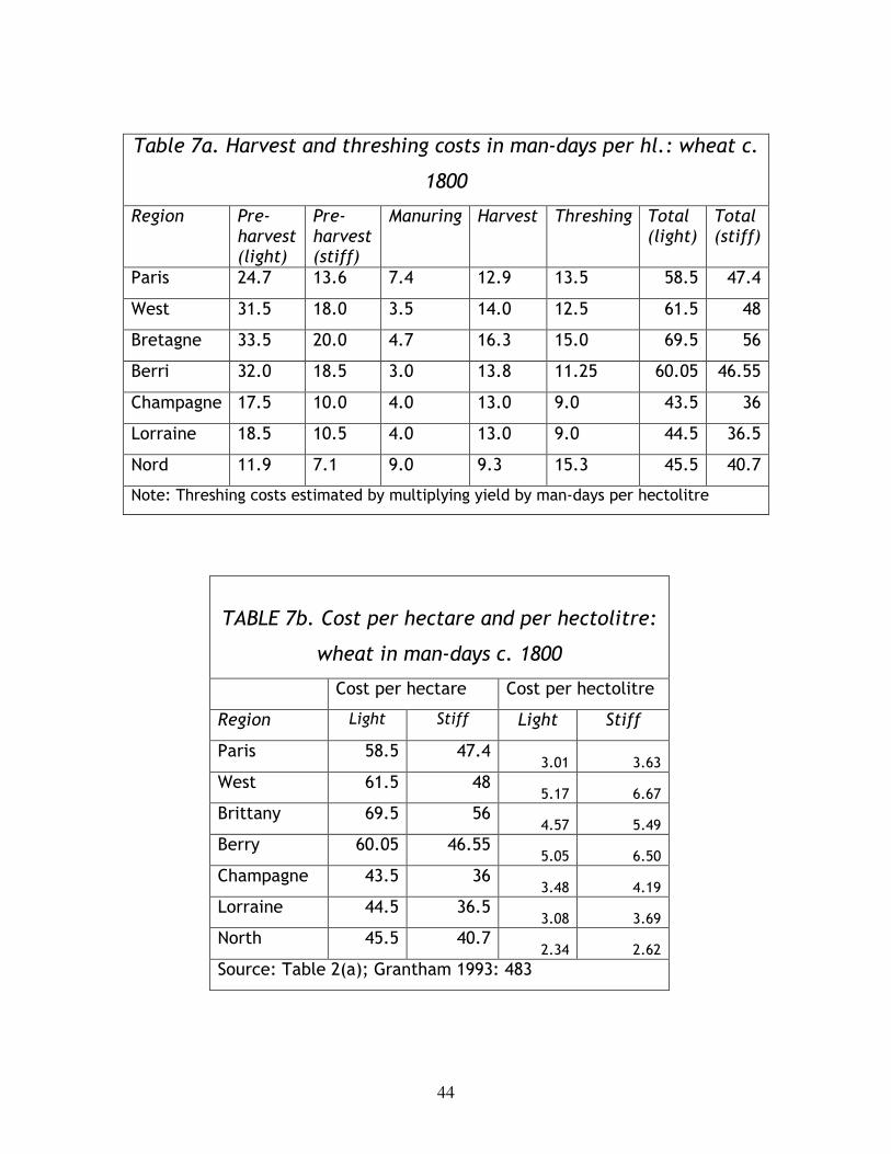
What of productivity? Grantham (1992: 362-63; 1993) has usefully
documented the number of man-days required to perform certain key tasks in
the cultivation and harvesting of wheat in seven French regions between the
eighteenth and twentieth centuries. These regions—which he defined as Paris,
29
Brittany, Berry, Champagne, West, Lorraine, and Nord—lay in the northern half
on France; in spatial terms they include about half of the hexagon. Here I
focus on three piece-rate measures provided by Grantham for the 1800-1850
period. The first measures the number of days it took to prepare the soil. The
second is the total cost in man-days of growing and harvesting a hectare of
wheat. The third is the cost in man-days of producing a hectolitre of wheat.
The distinction between the second and third measures matters because wheat
yields per hectare varied considerably across the seven regions. The
coefficient of variation of the cost per hectolitre was considerably higher than
that of the cost per hectare.
Some of Grantham’s estimates are summarized in Tables 7a and 7b.
They show that, calculated in terms of man-days per hectare, labour
productivity c. 1800 was highest in the Champagne, Lorraine, and Nord regions
and lowest in Brittany and the West. One would expect workers to have been
taller and better workers in the former regions than in the latter two centuries
ago. Were they?
[Tables 7a and 7b about here]
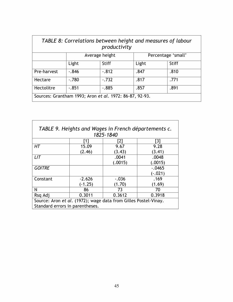
Data by département on the average height of conscripts recruited
between 1819 and 1826 and on the proportion who were deemed ‘small’ are
available (Aron et al. 1972: 92-93). In both cases regional height is taken to be
the arithmetic mean of the estimates for the relevant départements. Table 8
relates these heights data to Grantham’s measures of labour requirements in
30
the seven farming regions. The correlations between height and measures of
productivity are very high. They would be higher still if Brittany (where
productivity was high relative to height) was excluded. The implied elasticities
are huge, but we have not controlled for likely differences due to soil quality
(other than the distinction between ‘light’ and ‘stiff’), capital equipment, or
other forms of human capital.
The scatter-plot in Figure 9 describes the correlation between the
average heights of recruits in the 1820s and agricultural wages in 1840 across
départements (Aron et al. 1972; Le Roy Ladurie & Demonet 1980). Table 9
reports the results of regressing agricultural wages in 1840 (W40) on average
height (HT). We also use as explanatory variables the percentage literate
(LIT), and the percentage of recruits suffering from iodine deficiency (GOITRE).
The deleterious effects of iodine deficiency on health are well known; they
‘begin before birth [and] include detrimental effects on brain development,
stillbirths, increased infant and child mortality, and growth abnormalities’.
Today goitre is the leading preventable cause of mental retardation globally
(Sebotsa et al. 2003). We use natural log values of LIT and W40; the other
variables are measured as percentages. Table 4 suggests that LIT and GOITRE
have effects on W40 that are in the expected direction and independent of HT.
But after controlling for them, the implied impact of height on wages is still
significant; an elasticity value of 8, for example, means that a gap of about
one centimetre in height entailed a gap of about 5 per cent in wages, which is
similar (same order of magnitude) to the previous estimate in last section.
31
[Tables 8 and 9 about here]
Returning to English agriculture, Clark (1991: 449) estimated the cost of
reaping wheat from scattered but plentiful evidence in the reports prepared
for the officially funded Board of Agriculture in the 1800s. The average of the
forty-four observations found by Clark is 2.9 man-days per acre (or 7.2 days per
hectare). This estimate tallies with data collected by agronomist Arthur Young
on his agricultural tours of England over three decades earlier. Dividing the
median costs of reaping an acre of wheat (60d) by the median harvest wage
(20d-22d per diem) on both Young’s southern and northern circuits yields a rate
just short of three days per acre (Young 1771: IV, 293-96; 1772). Given that
piece-workers earned more than ‘the weekly pay of the country’ (1771: IV,
296), this calculation probably biases our estimate of the productivity of
harvest labour downwards. Young would probably not have objected to a rate
of 7 man-days per hectare. This indicates a considerable advantage over
France. In Grantham’s regions about this time the cost in man-days ranged
from 9.3 man-days per hectare in the relatively advanced Nord region to 16.3
man-days per hectare in economically backward Brittany. The average cost,
weighted by output share, was 12.9 man-days per hectare (Grantham 1992:
362).
Clark (1991: 449) similarly estimates the output of a day’s threshing at
0.236 man-days per bushel, which converts to 0.65 man-days per hectolitre.
32
Grantham’s estimates for his seven regions range from 0.9 man-days to 1.25
man-days per hectolitre, or nearly double the English rate.
In sum, England’s competitive ‘disadvantage’ in terms of time-rates on
the eve of the industrial revolution was matched, if not more than matched, by
its edge in output per unit of time. By this reckoning English wages, at least in
agriculture, were ‘high’ but labour was not ‘dear’. English workers were paid
more because they were stronger and more able.
5. CONCLUDING REMARKS
The past decade or so has seen a synergistic link developing between
economic history, on the one hand, and growth and development economics,
on the other. One by-product has been to push the search for the origins of
modern economic growth further back in time which, in turn, has led to
increased interest in the quantification of economic phenomena in the early
modern period. This paper is an extended comment on some of the resultant
data and their interpretation. It began by describing how new medieval English
demographic data implied a strong ‘Malthusian’ response to real wage shocks.
In seeking to reconcile medieval and later demographic regimes, it then
pointed to evidence for a rise in living standards in the pre-industrial era,
thereby casting some doubt on real wage time-series as a measure of trends in
living standards. Next, it explored, and found wanting, the asserted link
between living standards and climate change in the early modern era.
33
This rules out the need for a decline in food production and the diversion of
resources to keeping people warm as posited by supporters of a dramatic
cooling trend from the fourteenth century on. Finally, the paper drew
attention again to a second limitation of wage data. Comparative analysis of
height and work intensity seemed to confirm Clark’s reservations about wage
comparisons as gauges of relative competitiveness. It also reinforced the
implication that the English economy had been subject to differential
productivity growth in the pre-industrial era.
BIBLIOGRAPHY:
Aghion, Philippe, Peter Howitt, and Fabrice Murtin. 2009. ‘The Relationship Between Health and Growth: When Lucas Meets Nelson-Phelps’ [available at: http://www.economics.harvard.edu/faculty/aghion/papers_aghion].
Allen, R. C. 1992. Enclosure and the Yeoman: The Agricultural Development of the South Midlands 1450-1850. Oxford: OUP.
Allen, Robert C. 2002. ‘Labour Productivity in English Agriculture c. 1800’. http://eh.net/XIIICongress/cd/papers/85Allen248.pdf.
Allen, R.C. 2009. The British Industrial Revolution in Global Perspective. Oxford: OUP.
Apostolides, Alexander, Stephen N. Broadberry, Bruce M. S. Campbell, Bas van Leeuwen, & Mark Overton. 2008a. ‘Englsih GDP, 1300-1700: some preliminary estimates’. [available at: http://www2.warwick.ac.uk/fac/soc/economics/staff/academic/broadberry/wp/agriclongrun4.pdf]
Apostolides, Alexander, Stephen N. Broadberry, Bruce M. S. Campbell, Bas van Leeuwen, & Mark Overton. 2008b. ‘English agricultural output and labour Productivity, 1250-1850: Some Preliminary Estimates’ [available at: http://www2.warwick.ac.uk/fac/soc/economics/staff/academic/broadberry/wp/agricenglandmedieval.pdf].
34
Aron, Jean-Paul, Paul Dumont, & Emmanuel Le Roy Ladurie. 1972. Anthropologie du conscrit français. Paris: Mouton.
Barquin Gil, Rafael. 2005. ‘The elasticity of demand for wheat in the 14th to 18th centuries’. Revista de Historia Económica 23[2]: 241-268.
Becker, Gary S., Tomas J. Philipson, & Rodrigo R. Soares, 2005. ‘The Quantity and Quality of Life and the Evolution of World Inequality’. American Economic Review, 95[1]: 277-91.
Broadberry, Stephen N., Bruce M. S. Campbell, Alexander Klein, Mark Overton, & Bas van Leeuwen. 2009. ‘British economic growth, 1300-1850: some preliminary Estimates’ [available at: http://www.wehc2009.org/programme.asp?day=2&time=4].
Buttress, F. A., & R. G. W. Dennis. 1947. ‘The early history of seed treatment in England’. Agricultural History 21(2): 93-102.
Campbell, Bruce M. S. 2010. ‘Nature as historical protagonist: environment and society in pre-industrial England.” Economic History Review, forthcoming.
Campbell, Bruce M. S. Three Centuries of English Crops Yields, 1211-1491, URL http://www.cropyields.ac.uk.
Campbell, Bruce M. S. 2000. English Seigniorial Agriculture 1250-1450. Cambridge: CUP.
Campbell, Bruce M. S. 1983. ‘Agricultural progress in medieval England: some Evidence from Eastern Norfolk’. Economic History Review, 36(1): 26-46.
Campbell, B. M. S. 2005. ‘The agrarian problem in the early fourteenth century’. Past and Present. 188:3–70.
Campbell, B. M. S. and C. Ó Gráda. 2010. ‘Harvest shortfalls, grain prices, and famines in pre-industrial England’.
Clark, Gregory. 1987. ‘Productivity growth without technical change in European agriculture before 1850’. Journal of Economic History, 47(2): 419-432.
Clark, Gregory. 1989. ‘Productivity growth without technical change in European agriculture: reply to Komlos’. Journal of Economic History, 49(4): 979-991.
Clark, Gregory. 1991. ‘Yields per acre in English agriculture, 1250-1860: evidence from labour inputs’. Economic History Review. 44[3]: 445-60.
35
Clark, Gregory. 2007. ‘The Long March of History: Farm Wages, Population, and Economic Growth, England 1209-1869’. Economic History Review 60(1): 97-135.
Clark, Gregory. 2004. ‘The Price History of English Agriculture, 1209-1914’. Research in Economic History 22: 41-125.
Clark, G. 2007. Farewell to Alms. Princeton: PUP.
Chuine, Isabelle, Isabelle Yiou, Nicolas Viovy, Bernard Seguin, Valerie Daux and Emmanuel Le Roy Ladurie. 2004. ‘Grape ripening as a past climate indicator’. Nature 432(289–290).
Crébouw, Yvonne. 1986. ‘Salaires et salariés agricoles en France des débuts de la Revolution aux approches du XXe siècle’. Thèse d'histoire, Université de Paris I.
Darby, H.C. 2007. The Domesday Geography of Eastern England, 3rd. ed. Cambridge: CUP.
Dawson, A. G., K. Hickey, P. A. Mayewski and A. Nesje. 2007. ‘Greenland (GISP2) ice core and historical Indicators of complex North Atlantic climate changes during the fourteenth century’. The Holocene 17:427–434.
de Vries, Jan. 1980. “Measuring the impact of climate on history: the search for appropriate methodologies.” Journal of Interdisciplinary History, 10(4): 599-630.
De Vries, Jan. 1984. European Urbanization 1500-1800. London: Methuen.
de Vries, Jan. 2008. The Industrious Revolution: Consumer Behavior and the Household Economy, 1650 to the Present. Cambridge: CUP.
Dinda, Soumyananda, P.K. Gangopadhyay, B.P. Chattopadhyay, H.N. Saiyed, M. Pal, and P. Bharati. 2006. ‘Height, weight and earnings among coalminers in India’. Economics and Human Biology. 4(3): 342-350.
Dyer, Christopher. 1989. Standards of Living in the Later Middle Ages: Social Change in England C. 1200-1520. Cambridge: Cambridge University Press.
Ecclestone, Martin. 1999. ‘Mortality of rural landless men before the Black Death: the Glastonbury head-tax lists’, Local Population Studies, LXIII.
Fagan, Brian M. 2000. The Little Ice Age: How Climate Made History, 1300-1850. New York: Basic Books.
Fogel, R.W. 2004. The Escape from Hunger and Premature Death. Cambridge: CUP.
36
Forde, Lincoln E., Alvin J. Detterline, Kevin K. Ho, and Wenyuan Cao. 2000. ‘Gender- and height-related limits of muscle strength in world weightlifting champions’. Journal of Applied Physiology. 89: 1061-64.
Gao, Wenshu and Russell Smyth. 2009. ‘Health Human Capital, Height and Wages in China’. Working Paper, Monash University.
Grantham, George. 1991. ‘The growth of labour productivity in the production of wheat in the Cinq Grosses Fermes of France, 1750-1929’. In B.M.S. Campbell & M. Overton, eds. Land, Labour and Livestock: Historical Studies in European Agriculture. Manchester: MUP, pp. 340-63.
Grantham, George. 1993. ‘Divisions of labour: agricultural productivity and occupational specialization in pre-industrial Europe,’ Economic History Review 46(3): 478-502.
Habakkuk, H.J. 1962. American and British Technology in the Nineteenth Century: the Search for Labour-saving Inventions. Cambridge: Cambridge University Press.
Hatcher, J. A., J. Piper, and David Stone. 2006. ‘Monastic mortality: Durham Priory, 1395-1529’, Economic History Review. LIX: 667-87.
Hausman, Jerry. 1999. ‘Cellular telephone, new products, and the CPI’. Journal of Business and Economic Studies 17[2]: 188-94.
Hersh, Jonathan & H.-J. Voth. 2009. ‘Sweet diversity: colonial goods and the rise of European living standards after 1492’ [Available at SSRN: http://ssrn.com/abstract=1402322].
Houston, R.A. 1982. ‘The development of literacy: Northern England, 1640-1750’, Economic History Review, 35: 199-216.
James, Margery K. 1951’The fluctuations of the Anglo-gascon wine trade during the fourteenth century ‘. Economic History Review, n.s. IV(2): 170-96.
Kelly, Morgan, & C. Ó Gráda. 2010a. ‘Living Standards and Mortality in England since the Middle Ages: The Poor Law versus the Positive Check’, Unpublished.
Kelly, Morgan, & C. Ó Gráda. 2010b. ‘The end of the Little Ice Age’. Unpublished.
Kelly, Morgan, & C. Ó Gráda. 2010c. ‘The poor law of old England: resource constraints and demographic regimes’, Journal of Interdisciplinary History, forthcoming.
37
Koley, Shyamal, Navdeep Kaur & J.S. Sandhu. 2009. ‘A study on hand grip strength in female labourers of Jalandhar, Punjab, India’. Journal of Life Science, 1(1): 57-62.
Lamb, H. H. 1965. “The early medieval warm epoch and its sequel.” Palaeogeography, Palaeoclimatology, Palaeoecology 1: 13–37.
Lamb, H.H. 1995. Climate History and the Modern World. 2nd ed. London: Routledge.
Lee, R.D. 1981. 'Short-term variation: vital rates, prices and weather’, in Wrigley and Schofield, Population History of England.
Le Roy Ladurie, Emmanuel. 1971. Times of Feast, Times of Famine. London: Allen & Unwin.
Le Roy Ladurie, E. and M. Demonet. I980. 'Alphabetisation et stature: un tableau comparé', Annales E.S.C., xxxv: 1329-32.
Lindert, Peter H. & Jeffrey G. Williamson. 1982. ‘Revising England’s social tables, 1688-1812’, Explorations in Economic History 19[4]: 385-408.
Lucas, Robert. 1996. ‘The Industrial Revolution: past and future’. Estudios Públicos 64: 1-15.
Malthus, T.R. 1826. An Essay on the Principle of Population. London: John Murray, 6th edition.
McCloskey, D.N., & J. Nash. 1984. “Corn at Interest: The Extent and Cost of Grain Storage in Medieval England.” American Economic Review 74(1): 174-187.
Miskimin, Harry A. 1975. The Economy of Early Renaissance Europe, 1300-1460. Cambridge: Cambridge University Press.
Mitchell, Brian R. 1971. Abstract of British Historical Statistics. Cambridge: CUP.
Mokyr, Joel. 1976. Industrialization in the Low Countries. New Haven: Yale U.P.
Mokyr, Joel. 1991. "Dear Labor, Cheap Labor and the Industrial Revolution," in Henry Rosovsky and Patrice Higonnet, eds., Economic Growth: Constraints and Response (Cambridge, MA.).
Mokyr, Joel & C. Ó Gráda. 1996. ‘Height and Health in the United Kingdom 1815-1860: Evidence from the East India Company Army’, Explorations in Economic History, 33(2): 141-168.
38
Mokyr, Joel. 2010. The Enlightened Economy: An Economic History of Britain 1700-1850. New Haven: Yale University Press.
Neveux, Hugues, & Marie-Jeanne Tits-Dieuaide. 1979. ‘Étude structurelle des fluctuations courtes des rendements céréaliers dans l’Europe du Nord-Ouest (XIVe-XVIe siecle)’. Cahiers des Annales de Normandie 11: 17-42.
Nicholas, S. & R. Steckel. 1991. "Heights and living standards of English workers during the early years of industrialization", Journal of Economic History, 51: 937-957.
Nicolini, E. 2007. ‘Was Malthus right? A VAR analysis of economic and demographic interactions in pre-industrial England’. European Review of Economic History. 11: 99-121.
Ó Gráda, C. 2007. ‘Making famine history’. Journal of Economic Literature 45 (1): 3-36.
Olmstead, Alan L., & Paul W. Rhode. 2002. ‘The Red Queen and the Hard Reds: productivity growth in American wheat, 1800–1940’. Journal of Economic History 62(4), 929-966.
Page, Mark. 2003. ‘The peasant land market on the estate of the Bishopric of Winchester before the Black Death’. In The Winchester Pipe Rolls and Medieval English Society, ed. Richard Britnell. Woodbridge: Boydell.
Parkinson, Richard. 1811. General View of the Agriculture of the County of Huntingdon. London: Richard Philips.
Persson, Karl Gunnar. 1992. ’Labour productivity in medieval agriculture: Tuscany and the Low Countries’, in B.M.S. Campbell and M. Overton, eds. Land, Labour and Livestock, Manchester: MUP, pp. 124-43.
Persson, Karl Gunnar. 1999. Grain Markets in Europe, 1500-1900: Integration and Deregulation. Cambridge: CUP.
Persson, Karl Gunnar. 2010. An Economic History of Europe: Knowledge, Institutions and Growth, 600 to the Present. Cambridge: CUP.
Postan, Michael and J.Z. Titow. 1959. 'Heriots and prices on Winchester manors,' Economic History. Review, 11: 392-410.
Razi, Zvi. 1980. Life, Marriage and Death in a Medieval Parish: Economy, Society and Demography in Halesowen 1270–1400. Cambridge: CUP.
Roesdahl, Else. 1998. ‘L’ivoire de morse et les colonies norroises du Groenland’, Proxima Thule: Revue d΄Études Nordiques. 3: 9–48.
39
Rönnbäck, Klas. 2009. ‘Integration of global commodity markets in the early modern era’. European Review of Economic History, 13: 95-120.
Schultz, T.P. 2002. ‘Wage Gains Associated with Height as a Form of Health Human Capital’. American Economic Review, 92(2): 349-353.
Schultz, T.P. 2005. ‘Productive benefits of health: evidence from low-income countries’. IZA Discussion Paper No. 1482.
Seaver, Kirsten A. 2009. ‘Desirable teeth: the medieval trade in Arctic and African ivory’. Journal of Global History. 4:271-92.
Sebotsa, Masekonyela, Linono Damane, Andre Dannhauser, Pieter L. Jooste, & Gina Joubert. 2003. ‘Prevalence of goitre and urinary iodine status of primary–school children in Lesotho’, Bulletin of the World Health Organization. 81(1): 28-34.
Sen, A. K. 1981. Poverty and Famines: an Essay on Entitlement and Deprivation. Oxford: OUP.
Slutsky, Eugen E. 1937. ‘The summation of random causes as the source of cyclic processes’. Econometrica, 5: 105-46.
Snowdon, Brian. 2007. ‘Towards a unified theory of economic growth: Oded Galor on the Transition from Malthusian Stagnation to Modern Economic Growth’ [http://www.econ.brown.edu/fac/oded_galor/galor%20interview%20dec-17-2007.pdf].
Steckel, R. 2004. ‘New Light on the ‘‘Dark Ages’’: The Remarkably Tall Stature of Northern European Men during the Medieval Era’. Social Science History. 28:2: 211–29.
Strauss, John & Duncan Thomas. 1998. ‘Health, Nutrition, and Economic Development’. Journal of Economic Literature, 36(2): 766-817.
Thick, Malcolm. 1990. ‘Garden Seeds in England before the Eighteenth Century’. Agricultural History Review 38(2): 105-116.
Thomas, D. & Strauss, J. 1997. ‘Health and wages: evidence on men and women in urban Brazil’. Journal of Econometrics, 77: 159-185.
Titow, J. Z. 1969. English Rural Society 1200–1350. London: Allen & Unwin.
Turner, Michael E., John V. Beckett, and Bethanie Afton. 2001. Farm Production in England 1700-1914. Oxford: OUP.
Unger, Richard W. 2004. Beer in the Middle Ages and the Renaissance. Philadelphia: University of Pennsylvania Press.
40
Usher, Dan. 1973. ‘An imputation to the measure of economic growth for changes in life expectancy’, in M. Moss, ed. The Measurement of Economic and Social Performance, Chicago: University of Chicago Press, pp. 193-232.
van Engelen, A.F.V., J. Buisman & F IJnsen. 2001. “A Millennium of Weather, Winds and Water in the Low Countries.” In History and Climate: Memories of the future?, eds. P. D. Jones, A. E. J. Ogilvie, T. D. Davies and K. R. Briffa. Boston: Kluwer Academic. Also available at: http://www.knmi.nl/kd/daggegevens/antieke_wrn/millennium_of_weather.pdf.
van Zanden, Jan Luiten. 2009. The Long Road to the Industrial Revolution. The European Economy in a Global Perspective, 1000-1800. Leiden: Brill.
Williamson, J.G. 1984. ‘British mortality and the value of life, 1781-1931’, Population Studies 38: 157-72.
Wrigley, E.A. 1985. ‘Urban growth and agricultural change: England and the continent in the early modern period’, Journal of Interdisciplinary History, 15: 683- 728.
Wrigley, E. A., & R. S. Schofield. 1981. The Population History of England 1541-1871: A Reconstruction. London: Arnold.
Wrigley, E.A., Ros S. Davies, James E. Oeppen, and Roger Schofield. 1997. English Population History from Family Reconstitution. Cambridge: CUP.
Young, Arthur. 1771. A Six Months Tour through the North of England. 2nd ed. London: Strahan.
Young, Arthur. 1772. A Six Weeks Tour through the Southern Counties of England and Wales. 3rd ed. London: Strahan.
Young Arthur. 1793. Travels in France. Dublin. Cross et al.
41
Table 1: Effect of real wages and past mortality on inheritances, 1263–1348
Wage.
L1
Inherit.
L1
Inherit.
L2
1289
1317
1318
1342-44
‘R2’
Loglik
20 -.586
[.104]
.044
[.012]
.033
[.012]
.426
[.088]
.558
[.080]
-.483
[.117]
.323
[.063]
.473 -794
All -.485
[.091]
.027
[.008]
.018
[.007]
.418
[.078]
.600
[.069]
-.414
[.099]
.298
[.053]
.595 -1483
Multilevel Poisson regression of number of inheritances on lagged inheritances and real wages of agricultural labourers (in logs) by year from 1263 to 1348, with dummies for years of unusual mortality. Observations of lagged inheritances of zero are set to 0.001. There are 927 observations for the 20 largest manors, and 1,858 for the entire group of 66. ‘R2’ is the squared correlation between fitted and actual values. Intercepts not reported, se’s in parentheses.
Table 2: Likelihood of ‘back-to-back’ harvest failures, England 1268-1480
BACK-TO-BACK DEFICITS: WHEAT BARLEY OATS W-B-O Prob <90% of trend value 0.085 0.089 0.075 0.066 Average/Expected 1.140 1.088 1.127 1.350 Prob <80% of trend value 0.033 0.042 0.014 0.019 Average/Expected 1.089 1.872 0.945 1.479 Prob <70% of trend value 0.019 0.009 0.005 0.009 Average/Expected 2.360 1.664 0.832 6.656 THREE-IN-A-ROW DEFICITS WHEAT BARLEY OATS W-B-O Prob <90% of trend value 0.005 0.014 0.000 0.005 Average/Expected 0.465 1.599 1.636 1.305 Prob <80% of trend value 0.005 0.014 0.000 0.005 Average/Expected 0.896 4.154 0.000 3.282 Prob <70% of trend value 0.005 0.000 0.000 0.005 Average/Expected 6.615 0.000 0.000 88.61 Notes: The W-B-O column is a weighted average of net cereal yields, using the ratio 2:1:1. ‘Average/Expected’ is the ratio of actual to predicted frequency. The predicted frequency is set at the once-off probability of such a shortfall squared or cubed. Yield data from Campbell, Three Centuries.
42
Table 3. Gregory King on English incomes c. 1688
Population (M.) £ per head Y
Cottagers/paupers 1.018 2.0 2.04
Labourers/outservants 0.997 4.3 4.29
Others 3.684 13.1 48.26
Total 5.689 9.57 54.44
Source: Lindert and Williamson 1982
Table 4: England/Great Britain, annual variations in grain yields
Crop Period Country (1) Mean (2) σ (2)/(1)
Wheat 1268-1480 England 9.79 2.01 0.205
Barley 1268-1480 England 13.18 2.38 0.181
Oats 1268-1480 England 10.14 1.88 0.185
Wheat 1750-1850 England 22.61 2.80 0.123
Barley 1750-1850 England 33.42 4.64 0.130
Oats 1750-1850 England 38.69 7.70 0.199
Wheat 1884-1939 GB 31.26 2.227 0.071
Barley 1884-1939 GB 33.00 1.786 0.054
Oats 1884-1939 GB 40.14 1.810 0.045
Note: the standard deviations were estimated after the chronologies had been de-
trended using the Hodrick-Prescott filter. Yield data from Campbell, Three Centuries;
Turner, Beckett, and Afton, Farm Production (annual chronologies reconstructed from
original data supplied by the authors); Mitchell, British Historical Statistics, pp. 90-91.
43
Table 5. Cereal Yields and Weather, 1211-1500
Intercept Summer Rings Loglik R2 σα N Manors
Wheat 1.2227 ** 0.0503 ** -0.0565 ** -2389 .296 0.2042 8439 112
Rye 1.286 ** 0.0483 ** -0.0321 ** -597.2 .133 0.1372 1134 29
Barley 1.1805** 0.0035 -0.0087 ** -2231.4 .248 0.1934 7572 104
Oats 0.8742 ** 0.0201 -0.0042 -2648.2 .152 0.1417 8290 116
Mixed effects regression of log cereal yield ratio on estimated summer temperatures (deviation from mean value of 15.3 Celsius) and oak ring thickness. Intercept varies across manors: σα is its standard deviation. N is number of observations and Manors is the number of manors. R2 is the pseudo-R2 for each regression. * denotes significance at 5 percent, ** at 1 percent.
Table 6: Summary statistics for annual weather until 1900
Start Mean SD ρ SE R2 L-B
Temperature English Summer 1660 15.26 0.79 0.102 0.065 0.010 0.111 English Winter 1660 3.49 1.35 -0.031 0.065 0.001 0.626 Dutch Summer 1200 16.25 0.93 0.121 0.038 0.015 0.001 Dutch Winter 1200 1.73 1.62 -0.031 0.038 0.001 0.410 Burgundy Summer 1340 -0.09 0.98 0.152 0.043 0.023 0.000 N. Hemisphere 1200 -0.14 0.12 0.615 0.03 0.38 0.000 Rainfall English Summer 1720 444.93 87.79 0.114 0.087 0.013 0.183 English Winter 1720 461.89 86.21 0.02 0.087 0.000 0.182 Oak Rings 1200 0.02 1.00 0.331 0.036 0.109 0.000 Mean, standard deviation, and autoregressive coefficient, standard error and R2 for historical weather series. L-B is the p-value of the Ljung-Box test for randomness.
44
Table 7a. Harvest and threshing costs in man-days per hl.: wheat c.
1800
Region Pre-harvest (light)
Pre-harvest (stiff)
Manuring Harvest Threshing Total (light)
Total (stiff)
Paris 24.7 13.6 7.4 12.9 13.5 58.5 47.4
West 31.5 18.0 3.5 14.0 12.5 61.5 48
Bretagne 33.5 20.0 4.7 16.3 15.0 69.5 56
Berri 32.0 18.5 3.0 13.8 11.25 60.05 46.55
Champagne 17.5 10.0 4.0 13.0 9.0 43.5 36
Lorraine 18.5 10.5 4.0 13.0 9.0 44.5 36.5
Nord 11.9 7.1 9.0 9.3 15.3 45.5 40.7
Note: Threshing costs estimated by multiplying yield by man-days per hectolitre
TABLE 7b. Cost per hectare and per hectolitre:
wheat in man-days c. 1800
Cost per hectare Cost per hectolitre
Region Light Stiff Light Stiff
Paris 58.5 47.4 3.01 3.63
West 61.5 48 5.17 6.67
Brittany 69.5 56 4.57 5.49
Berry 60.05 46.55 5.05 6.50
Champagne 43.5 36 3.48 4.19
Lorraine 44.5 36.5 3.08 3.69
North 45.5 40.7 2.34 2.62
Source: Table 2(a); Grantham 1993: 483
45
TABLE 8: Correlations between height and measures of labour productivity
Average height Percentage ‘small’
Light Stiff Light Stiff
Pre-harvest -.846 -.812 .847 .810
Hectare -.780 -.732 .817 .771
Hectolitre -.851 -.885 .857 .891
Sources: Grantham 1993; Aron et al. 1972: 86-87, 92-93.
TABLE 9. Heights and Wages in French départements c. 1825-1840
[1] [2] [3] HT 15.09
(2.46) 9.67 (3.43)
9.28 (3.41)
LIT .0041 (.0015)
.0048 (.0015)
GOITRE -.0465 (-.021)
Constant -2.626 (-1.25)
-.036 (1.70)
.169 (1.69)
N 86 73 70 Rsq Adj 0.3011 0.3612 0.3918 Source: Aron et al. (1972); wage data from Gilles Postel-Vinay. Standard errors in parentheses.
46
Figure 1. Real Wages in Agriculture, 1200s-1860s
20
40
60
80
100
120
140
1200 1300 1400 1500 1600 1700 1800
1860s=
100
Source: Clark 2007: 99-100
Fig. 2. Wage and GDP per Head 1300-1700
50
100
150
200
250
300
1300 1350 1400 1450 1500 1550 1600 1650 1700
Source: Apostolides et al. (2008); Clark (2005)
WAGE
W/Y
Y
47
Note: the mean annual difference is calculated as the mean percentage year-to-year change in the logged wheat price, averaged over half-centuries; the prices for Amsterdam, Bruges, Cologne, London, Paris, Pisa, Strasbourg, Madrid, Valencia, and Vienna are those given in the Allen—-Unger Database. Figure 3: Wheat price: mean annual percentage change in ten European urban markets, 1300-1899.
48
Note: the mean annual difference is calculated as the mean percentage year-to-year change in the logged wheat price, averaged over half-centuries; the prices for England, London, Exeter, and Eton are those given in Allen and Unger, Allen—-Unger Database. To highlight how anomalous are the sixteenth-century figures, they have been excluded from the polynomial. Figure 4: Wheat price: mean annual percentage change in England and three English urban markets, 1260-1914.
Figure 5. Urbanization in France and England, 1500-1800
0
5
10
15
20
25
1500 1550 1600 1650 1700 1750 1800
%
France
England
49
te
mp
de
v
year1370 1900
-2.3
4.1
-2.3
4.1
tempdev
1370-991400-49
1450-991500-49
1550-991600-49
1650-991700-49
1750-991800-49
1850-99
Figure 6[a]. Burgundy Grape Harvest Index, 1370-2000
win
ter
year1300 1900
-31
53
-31
53
w inter
1300-491350-99
1400-491450-99
1500-491550-99
1600-491650-99
1700-491750-99
1800-491850-99
Figure 6[b]. Low Countries Winter Temperatures, 1300-2000
sum
mer
year1300 1900
131
189
131
189
summer
1300-491350-99
1400-491450-99
1500-491550-99
1600-491650-99
1700-491750-99
1800-491850-99
Figure 6[c]. Low Countries Summer Temperatures, 1300-2000
50
mann
year1600 1900
-.442
.122
-.442
.122
mann
1600-49 1650-99 1700-49 1750-99 1800-49 1850-99
Figure 6[d]. Mann et al., 1600-1990
Sw
itzerl
and
year1500 1900
-1.39444
.845722
-1.39444
.845722
Sw itzerland
1500-491550-99
1600-491650-99
1700-491750-99
1800-491850-99
Figure 6[e]. Switzerland, 1500-1900
Argentiere, 1600-2000
-1400
-1200
-1000
-800
-600
-400
-200
0
200
400
600
800
1600 1650 1700 1750 1800 1850 1900 1950 2000
U. Grindelwald, 1534-1980
-2000
-1500
-1000
-500
0
500
1000
1534 1584 1634 1684 1734 1784 1834 1884 1934
Rhonegletscher 1600-2000
-2500
-2000
-1500
-1000
-500
0
1600 1650 1700 1750 1800 1850 1900 1950 2000
[a] Argentière [b] U. Grindelwald [c] Rhonegletscher
Figure 6[f]. Glacier Lengths, 1500-2000
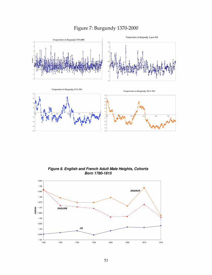
51
Figure 7: Burgundy 1370-2000
Temperature in Burgundy 1370-2000
-3
-2
-1
0
1
2
3
4
5
1370 1470 1570 1670 1770 1870 1970
de
via
tio
ns
Temperature in Burgundy, 5-year MA
-1.5
-1
-0.5
0
0.5
1
1.5
2
2.5
1375 1475 1575 1675 1775 1875 1975
Temperature in Burgundy, 25-Yr MA
-0.8
-0.6
-0.4
-0.2
0
0.2
0.4
0.6
0.8
1395 1495 1595 1695 1795 1895
Temperature in Burgundy, 50-Yr MA
-0.5
-0.4
-0.3
-0.2
-0.1
0
0.1
0.2
0.3
0.4
0.5
0.6
1430 1530 1630 1730 1830 1930
Figure 8. English and French Adult Male Heights, Cohorts Born 1780-1815
1.64
1.645
1.65
1.655
1.66
1.665
1.67
1.675
1.68
1.685
1.69
1.695
1780 1785 1790 1795 1800 1805 1810 1815
metr
es
ENGRUR
ENGURB
FR
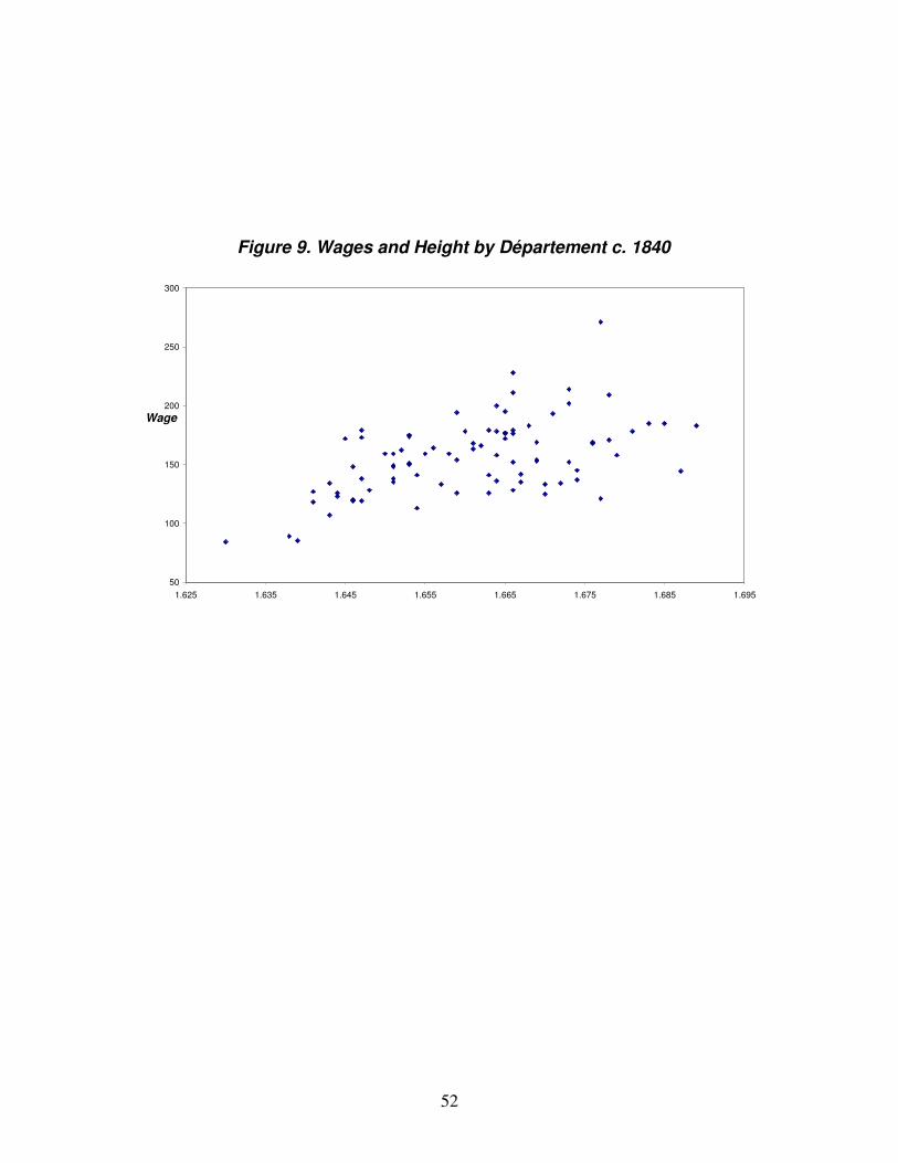
52
Figure 9. Wages and Height by Département c. 1840
50
100
150
200
250
300
1.625 1.635 1.645 1.655 1.665 1.675 1.685 1.695
Wage