Poor Little Children: The Socioeconomic Gap in

Parental Responses to School Disadvantage∗

Ines Berniell† Ricardo Estrada‡

February, 2019

Abstract

This paper studies how parents react to a widely-used school policy that puts

some children at a learning disadvantage: age at school entry. In specific, we

analyze Spanish data on parental investment and find that college-educated parents

increase their time investment and choose better schools when their children are

the youngest at school, while non-college educated parents do not. Consistent with

the increase in parental investment, we document a lower month of birth penalty

among children with college-educated parents.

Keywords: parental investment, age at school entry, education inequality, compensating

behaviour.

JEL Classification: I20, D10

∗Acknowledgments: We thank Manuel Bagues and Andrea Ichino for detailed comments. We alsothank Lian Allub, Fabrizio Bernardi, Lucila Berniell, Gabriel Fachini, Gabriela Galassi and the audiencesat the Universidad de Buenos Aires, CAF, EUI Microeconometrics Working Group, the EUI Max WeberConference, the IEA World Congress at CIDE, the Meeting of the Impact Evaluation Network, theCORE Annual Meeting, the IZA Economics of Education Workshop, NAMES at Washington Universityin St. Louis, AAEP and LACEA in ESPOL for valuable insights. We are grateful to Marta Encinasand Francois Keslair for their expertise and help with handling OECD data and to the Max WeberProgramme at the EUI for funding during the start of this project. All errors are our own.†CEDLAS (Center for Distributional, Labor and Social Studies), Universidad Nacional de La Plata,

Calle 6 Nro. 777, La Plata, Argentina, email: ines.berniell@econo.unlp.edu.ar.‡CAF-Development Bank of Latin America, Avenida Madero 900, Piso 15, Torre Catalinas Plaza,

Ciudad de Buenos Aires, Argentina, email: restrada@caf.com.

0

1 Introduction

Life (policy) can put some children at a disadvantage. If this is the case, parents can react

to disadvantage by changing their investment in their children and, potentially, mitigate

it. However, parental reactions might depend on parental resources, with important

implications for inequality and social mobility and for policy impacts. Our understanding

of such responses is limited, however, because a proper empirical analysis requires both

exogenous variation in exposure to disadvantage and the availability of detailed data on

parental investment.

In this paper, we get around these limitations by looking at a variation in exposure

to school disadvantage that is both well documented as potentially exogenous and easy

to observe across datasets, including those with information on parental investment. In

specific, we use time-use surveys and school-based questionnaires to study how parents

from different socioeconomic statuses (SES) react to a widely-used school policy that

puts some children at a learning disadvantage: the age at school entry.

Most countries dictate that children born during a given one-year period should start

school at the same time. This (up to one-year) difference in the age of students in the

same classroom can be reflected in performance. For instance, younger children might

be less ready to acquire knowledge and, overall, to deal with the experience of formal

schooling. If initial outcomes shape future outcomes, the age at school entry can have

long-term consequences for schooling and labour market trajectories (see Subsection 2.1).

A large body of literature shows that starting school at an earlier age is indeed re-

lated to worse student performance, labour market outcomes, and criminal behaviour.1

Furthermore, this negative effect might be greater among people from a disadvantaged

background, at least in some contexts (see Attar and Cohen-Zada, 2017 on Israel, Gratz

and Bernardi, 2017 on England, Fredriksson and Ockert, 2014 on Sweden and McEwan

and Shapiro, 2008 on Chile).2

Before looking at potential differences in parental investments, we first document that

younger children tend to perform worse in school than older children in Spain. Using

data from four waves of the PISA survey, we find that students who started school at

a younger age are more likely to have repeated a grade and to have lower test scores in

mathematics and reading at age 15 than their older peers. For example, students born

in December (the youngest in their cohort) are 10 percentage points more likely to have

1For student outcomes, see for example: Bedard and Dhuey, 2006 and Elder and Lubotsky, 2009 onthe United States; Muhlenweg and Puhani, 2010 on Germany; Grenet, 2011 on France. For the effecton the probability of ADHD diagnoses: Schwandt and Wuppermann, 2016; Elder, 2010. For criminalbehaviour: Cook and Kang (2016) and Landersø, Nielsen, and Simonsen, 2016 on the United States andDenmark, respectively. For labour market outcomes: Fredriksson and Ockert, 2014 on Sweden; Bedardand Dhuey, 2012 and Dhuey and Lipscomb, 2008 on the United States; and Black et al., 2011 on Norway.The latter document that this age effect on earnings dilutes when people reach 30 in Norway.

2Elder and Lubotsky (2009), in contrast, find opposite results in the United States.

1

repeated a grade at age 15 than those born in January (the oldest).3 We go further and

explore how this pattern translates into long-term outcomes, using information from the

Spanish population census. We find that adults who were younger at school entry have

less schooling and less educated partners.

A causal interpretation of the documented age effect requires that 1) parents do not

manipulate their child’s effective age of school entry (by postponing enrollment for one

year); and 2) there is no connection between the characteristics of newborns and their

month of birth. Some parents might be willing to enroll their children in school later

than regular entry if they are sufficiently concerned about the negative effects associated

with the age at school entry.4 Spain enforces a strict birthday cut-off for school entry, so,

even if they wish to, parents cannot opt for strategy 1) (see Section 2.2). Alternatively,

there could be a connection between the characteristics of newborns and the month of

birth if parental characteristics or relevant environmental (institutional) conditions that

shape fetal (newborn) health vary during the year.5

We analyze the birth certificates from the universe of newborns in Spain from 2007

to 2014 to study potential seasonality in births.6 Using census-type data allows us to

detect birth patterns that could go unnoticed in survey data because of a small sample

size. We find that there is indeed some seasonality in births. However, and this is key

for a causal interpretation, we do not find significant differences in the characteristics of

babies born in December and January (just before and after the birthday cut-off for entry

to school, which is January 1st). We confirm this pattern by looking at differences in

parental characteristics between people born in December and January, in the datasets

used in our main analysis.

We, therefore, focus our analysis on people born in January (the oldest at school

entry) and December (the youngest).7 Using data from PISA, we show that the effect of

the age of school entry is significantly larger among children from disadvantaged fami-

lies. For instance, young students from low-SES families are 12.7 percentage points more

likely to have repeated a grade at age 15 than older students from the same socioeco-

nomic background. This gap is only 4 percentage points among students from high-SES

families.8

To analyse whether this difference is related to parental investment according to family

background, we assemble two different datasets with detailed information about parental

3This pattern echoes the findings of Calsamiglia and Loviglio (2016) on Catalonia.4Dhuey, Figlio, Karbownik, and Roth, 2017 document that postponing school enrollment is a common

practice in the United States.5Along these lines, Buckles and Hungerman (2013) documents seasonality in maternal characteristics

in the United States.62007 is the first year in which parental characteristics are available in the birth certificate data.7Across datasets, we focus our basic specification on people born in January and December of the

same calendar year. However, when data is available, we compare individuals born in adjacents Januaryand December months and find similar results (available in Online Appendix).

8This result is robust to using both binary and continuous specifications of the SES index.

2

investment: the two waves of the Spanish Time Use Survey (2003 and 2009, STUS)

and the General Diagnostic Assessment (a national evaluation of 4th grade students

undertaken in 2009, GDA, which has information about parental involvement and school

characteristics).9 Our focus on parental time investment in child development is grounded

in the literature which shows that parental time input is important for the cognitive

development of their children, particularly when they are young (Del Boca, Flinn, and

Wiswall, 2014). We find that college-educated parents increase the amount of time they

spend helping their children with school activities and that they choose schools with

better inputs when their children are the youngest at school entry, while parents without

a college education do not. Specifically, we find that college-educated parents spend on

average five more minutes per day helping their children with school activities when their

children are the youngest at school entry, a result that is s tatistically significant at the five

percent level. This is a large effect. In context, parents in our sample spend on average

7.5 minutes per day helping their children with school activities. This effect increases to

10 minutes per day when we focus in children 6 to 12 years old, the age window in which

parental help in school chores is concentrated (and averages 12.5 minutes per day) and to

15 minutes per day when we exclude summer. Supporting the idea that the differences in

parental time investment are related to what happens at school, we do not observe that

parents spend more time doing learning activities with their younger children when they

are of pre-school age.

Finally, we deepen our analysis by looking at gender differences. Here, we find sug-

gestive evidence of different gender patterns among children from high-SES families. On

the one hand, younger boys from high-SES families do not seem to be able to overcome

the school entry age disadvantage by the age of 15, and probably because they face a

larger disadvantage they receive more parental help with homework and other academic

activities, and are more likely to attend schools with better inputs. On the other hand,

younger girls from high-SES families do not have different achievement levels at age 15

to their older peers, and probably because they face a smaller disadvantage, they do re-

ceive more parental time than older girls from the same SES families, but attend similar

schools. We find no such gender specific effect among children from low-SES families.

Our results highlight the importance of considering behavioral responses to policy

for the impact evaluation literature based on reduced-form estimates. The reduced-form

effects of a policy include both a direct (policy) effect and an indirect effect consisting of

endogenous responses to the policy - in our case, parental responses to the school-entry

9To interprete differences in parental investment by month of birth and SES as differences in parentalresponses by SES to school disadvantage requires that the relationship between parental inputs and age(month of birth) only varies by SES because the age at school entry penalty. The main concern herewould be that low-SES parents decrease faster their time investment than the high-SES parents as theirchildren grow older–this is less of a concern to study responses related to school choice. We show though,in Section 4.4, supporting evidence for this identification assumption.

3

age (Todd and Wolpin, 2003). To disentangle policy effects and production function

parameters, we need to understand behavioural responses to policies. Specifically, we

contribute to the emerging literature on parental reactions to school policies (see Das

et al., 2013; Fredriksson et al., 2016; Pop-Eleches and Urquiola, 2013).10 We contribute

to this literature by highlighting how these reactions might vary according to parental SES

and student’s gender, and by providing more detailed evidence on parental responses. In

the closest study to ours, Fredriksson et al. (2016) show that larger class sizes in Sweden

increase the likelihood that high-income parents help their children with their homework

and low-income parents move their children to a different school. Relative to this paper,

we make two contributions. First, we use richer measures of parental investment, which

allows to quantify the magnitude of changes in parental time investment, to obtain a

more comprehensive picture of changes in school inputs, and to analyze how responses

in parental time investments evolve over their children’s life cycle. Second, we look at

whether parental responses depend on the interaction between parental SES and their

children’s gender.11

We also contribute to the ample literature on the effects of age at school entry. Here,

we provide novel evidence on a plausible mechanism behind the heterogeneous effect of

age at school entry according to SES: differences in parental investment in terms of time

and school choice. In a contemporaneous work, Dhuey et al. (2017) use data from the

state of Florida in the United States to show that high-SES parents are more likely than

low-SES parents to postpone the enrollment of their children in school by one year (a

possible practice in that context). Their results support our findings: high-SES parents

are more likely to help their children when they are among the youngest at school entry.

The rest of the paper is organized as follows. Section 2 elaborates on the relationship

between age at school entry and student outcomes, and describes the institutional frame-

work. Section 3 presents the data and Section 4 the identification strategy. Section 5

describes the results for age at school entry, and Section 6 analyses of parental responses

and the differences in these responses according to the child’s age and gender. Section 7

concludes.

10On the thoretical side, Albornoz et al. (2018) develop a model in which parents compensate for lowereducational quality, i.e. public and private investments in a child’s human capital are substitutes.

11A related literature analyses how parental investment responds to health endowment at birth. Manyempirical studies seem to find evidence suggesting that parental investment reinforces initial differencesin health endowments, although there are some indications that high-income parents might be moreprone to compensating behavior (see the literature review in Almond and Mazumder, 2013).

4

2 Age at School Entry

2.1 How Can Age at School Entry Affect Schooling Outcomes?

The specialized literature has devoted much attention to the issue of how age at school

entry can affect student (and adult) outcomes (see, for example, Crawford et al., 2007).

These effects are typically categorized as 1) age at starting school, 2) age at testing, 3)

relative age and 4) length of schooling.

1. As age is a determinant of maturity, younger children at school entry might be

less ready to acquire knowledge and, overall, to deal with the experience of formal

schooling (Dhuey, 2016). Moreover, because of their age, older students are more

likely to have accumulated a higher stock of skills at school entry than their younger

classmates, which could also help them to learn more in school.

2. If all the children in a school cohort are examined on the same day, then students

are examined at different ages and some students are always younger than their

peers.

3. Younger students might perform worse because they are younger than their peers

if, for example, differences in absolute performance due to maturity affect the ac-

cumulation of skills like self-confidence.

4. The time students spend in the education system might depend on regulations

about the timing when students can enter (leave) formal schooling.

The relevance of these effects in shaping student and adult outcomes might depend on

the structure of the education system. For example, the level of maturity at school entry

is likely to be more important in countries that teach the same (ambitious) curriculum

to all students independently of their achievement levels – as is the case in Spain. The

same story goes for contexts where grade retention is commonly used - such as Spain.

Younger – and less mature – students might be more likely to repeat a grade, which

might be detrimental to them if it is associated with negative stereotypes or a loss of self-

esteem. The use of (rigid) tracking based on early achievement levels might set younger

students on different educational trajectories – ones with access to fewer school inputs –

than their older peers (Muhlenweg and Puhani, 2010). Similarly, age at testing can affect

educational trajectories if grades or other measures used to assess student performance

are not adjusted for age. Grenet (2011) gives a more complete discussion of how the

structure of education systems can amplify initial differences in performance due to age

at school entry.

Summing up, their greater maturity and larger human capital at school entry, i.e.

higher school readiness, can lead older students to perform better initially. If early learn-

5

ing is complementary to later learning (dynamic complementarities) this initial difference

in learning outcomes could place early entrants at a permanent disadvantage.

2.2 Institutional Framework

2.2.1 Age at School Entry

In Spain, children must begin primary school in the September of the calendar year of their

6th birthday. This is an inflexible rule. The birthday cut-off to enter school is January

1st and children are not allowed to postpone entry to school (IEA, 2011). Although it is

not compulsory, almost every child attends kindergarten from the September of the year

of their third birthday. To illustrate the inflexibility of the Spanish birthday cutoff, we

look at children born up to one year before and after a given school birthday cutoff and

see if they attend either kindergarten or primary school. To do so, we rely on data from

the 2008 to 2016 waves of the Life Conditions Survey (LCS, Encuesta de Condiciones

de Vida in Spanish). This survey is carried out by the Spanish National Institute of

Statistics (INE by its Spanish acronym) to gather data on household characteristics.12

Figure 1 plots the percentage of children enrolled in kindergarten and primary school by

month of birth, stacking the 10 birth cohorts available in our data. As it is evident from

the graph, compliance with the birthday cutoff rule is strict. Official enrollment statistics

confirm this pattern: only 0.5 percent of chidren who have reached the statutory age for

entry into primary education are enrolled in pre-primary education (Eurydice, 2011).

2.2.2 Grade Retention

Grade repetition is allowed and common. Students can be obliged to repeat a grade once

during primary education (grades 1-6), although some exceptions apply for students with

special needs, who can be retained twice. Students can repeat (both) grades 7 and 8;

although the total number of repeated years is limited to two in grades 1 to 8. Grade

retention is a common practice in both primary and lower secondary school. In fact,

Spain is among the three OECD countries with the highest rates of repetition at the

primary level (the others are France and Portugal). Similarly, almost a third of students

in lower secondary school repeat at least one grade – in contrast to only 0.5% of students

in Finland (Eurydice, 2011). Thus, grade retention seems to be commonly used as a

remedy for pupils in difficulty in primary and lower secondary education.

12This is the only publicly available dataset we could find with information on both schooling atten-dance and month of birth for children aged 5 to 6 years old.

6

Figure 1: School Enrollment by Schooling Level and Month of Birth: Children 5 and 6years old

5 years old 6 years old

0

20

40

60

80

100

Per

cent

age

of s

tude

nts

(%)

Jan

Feb

Mar

Abr

MayJun

Jul

Aug

SepOct

Nov

DecJan

Feb

Mar

Abr

MayJun

Jul

Aug

SepOct

Nov

Dec

Date of birth

Go to primary school Go to kindergarten

Notes: Data from the 2008 to 2016 waves of the Spanish Life Conditions Survey. The figure plots the percentage

of children enrolled in kindergarten and primary school by month of birth. 95% confidence intervals are

reported.

2.2.3 School Choice

School choice in primary and secondary education is available in Spain since the 1980s.

In principle, parents can choose any public or semi-public (concertada) school in their

municipality of residence for their children to attend. A national law supplemented by

province (autonomous-comunity) regulations dictate the procedures to deal with excess

demand for schools. Typically, parents can list a (limited) number of schools in order

of preference. Then, central authorities allocate children to schools using an algorithm

equivalent to the Boston mechanism, with priorities given on basis of neighborhood of

residence, sibling status and socioeconomic characteristics (see details in Calsamiglia,

2014).

3 Data

We analyze data from five different sources. We use micro data from Spanish birth

certificates to study birth seasonality. We rely on data from the OECD Programme for

International Student Assessment (PISA) and the Spanish population census to analyse

the medium- and long-term impacts of the school entry age, respectively. The PISA data

also allows us to look at socioeconomic differences in the effect of being younger at school.

To analyse the potential mechanisms explaining these socioeconomic differences, we use

two different surveys with information about parental investment: the 2009 General

Diagnostic Assessment (GDA, Evaluacion General de Diagnostico in Spanish) and the

7

Spanish Time Use Survey (STUS). We use the first of these surveys to study school

characteristics and parental help with homework, and the second to study parental time

spent on monitoring, teaching and helping children with school-related tasks.

We restrict the analysis of all the datasets to the individuals born in Spain, because

seasonality in births (an important element for our identification strategy) can vary across

countries.

3.1 Spanish Birth Certificates

We use micro data from the universe of Spanish birth certificates from July 2007 to

June 2014. The Spanish National Statistical Institute compiles this dataset using the

standardized form that families hand in at the time of birth registration. The dataset

includes detailed information about the newborn baby (birth weight, method of deliv-

ery, gender, an indication of premature birth, among others) and parental demographic

characteristics.

We use data starting from 2007 because the information about parental education is

only available from that year onwards. We exclude the last semester of 2010 and the

first semester of 2011 because Borra, Gonzalez, and Sevilla (2015) show that a temporary

policy (a cash transfer) implemented in these years induced changes in birth seasonality.

We have 2,462,991 observations in the years included in the analysis and we are left with

2,275,737 (92%) after taking into consideration missing values in the variables of interest.

Table A.1 reports summary statistics.

3.2 Programme for International Student Assessment

PISA is an international survey run by the OECD that assesses the skills and knowledge

of 15-year-old students. We use Spanish data from the 2003, 2006, 2009 and 2012 waves

to analyse the relationship between age at school entry and academic performance at

age 15, and to study how this relationship varies with family background. In addition

to test scores in mathematics and language and data on grade repetition, the survey

has information on student socioeconomic characteristics: indices of economic, social and

cultural status, parental education, and birthday among others.13 We obtain a data set

with 75,082 observations after pooling the four waves of PISA, from which we keep 74,832

(99.7%) after dropping observations with missing values. Table A.2 shows the summary

statistics of the sample analysed.

13PISA 2006, 2009 and 2012 included an optional questionnaire for parents. However, it was notcarried out in Spain.

8

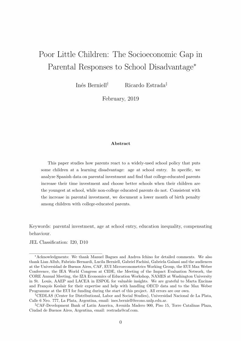
3.3 Spanish Population Census

We use micro data from the 2011 Spanish population census. We download the dataset

(10% random sample) from the IPUMS project website, which collects harmonized census

data from around the world. We restrict the sample to individuals aged between 30

and 55 at the moment of the census. The database includes information about the

individual’s education, employment status, marriage status, partner’s education (for those

married) and month of birth. We obtain a total of 1,437,574 observations and 1,373,194

(95,5%) after leaving out observations with missing values. Unfortunately, the census

questionnaire does not include questions about parental background. Table A.3 reports

summary statistics.

3.4 General Diagnostic Assessment

The Spanish Ministry of Education ran the GDA in 2009 with the purpose of evaluating

the general competences of students in grade 4. As part of the assessment, a random

sample of grade 4 students took standardized tests in 4 subjects (mathematics, reading,

science and civic education), while parents, pupils and school principals answered ques-

tionnaires. Our outcomes of interest are mainly those related to parental investment in

their children’s education. We use information from the surveys of students and parents

on whether parents help their children with doing homework, check students’ homework

and attend school meetings. To analyse parental investment through school choice, we

use information on school characteristics (public or private school, class size, teacher pro-

file, etc.) from the survey of school principals (who assess how motivated students and

parents in the school are).

The dataset includes information on students’ birthdays and we use maternal educa-

tion (an indicator of whether the mother has a college degree) as a proxy for household

socioeconomic status. 887 schools were selected to participate in the study, which cov-

ered all fourth-grade students in these schools. The GDA dataset contains 21,738 student

observations and 18,583 (85.5%) after taking into account missing responses. Table A.4

shows summary statistics.

3.5 Spanish Time Use Survey

We use data from the two waves of the Spanish time use survey (2003 and 2009). Each

survey includes a representative sample of the Spanish population. We use information

from the diaries of activities reported by all household members older than 10. Each

household member older than 10 fills out a diary in which she reports her activities

across the previous 24 hours, at 10 minute intervals. They also report whether a child

aged 0–9 or another member of the household was present during the activity.

9

Our outcomes of interest are the time parents spent with their children on the follow-

ing activities: teaching, reading and playing, and other childcare activities. We construct

these variables by adding up the total time that parents report spending on these cat-

egories according to their child’s age (0 to 9, and 10 to 17 years old). We also have

information on individuals’ months of birth and their mothers’ education (an indicator of

whether the mother has a college education). The sample analysed includes households

with children (individuals younger than 18). This amounts to 6,286 households in 2003

and 2,356 in 2009. We are left with a total sample of 13,045 children (96.8%) after taking

into account missing responses in the variables of interest. Table A.5 shows summary

statistics.

4 Empirical Strategy

This section presents our empirical approach to analyze how the age at which children

begin school affects their performance (at school and also in long-term outcomes), and,

more importantly, to study how parents react to this age gap.

4.1 Month of birth and medium- and long-term outcomes

We start by providing evidence on the relationship between the month of birth and

student outcomes. Using data from PISA, Figure 2 shows local means of grade repetition

and test scores at age 15 by month of birth. There is a clear monotonic relationship

between these variables. People born later in the year – and hence who are younger at

school entry – tend to perform worse at school, both in terms of grade repetition and test

scores. The size of the differences in academic performance between the youngest and

the oldest children is large. For example, students born in December (the youngest) are

around 10 percentage points more likely to have repeated a grade at age 15 than those

born in January (the oldest); and to have test scores around 0.1 standard deviations (SD)

lower in both mathematics and reading. These differences are similar to the gender gap

observed in this dataset.

We then use the population census to look at the relationship between the month of

birth and long-term outcomes. Figure 3 shows local means of the probability of having a

college degree by month of birth. In contrast to the PISA data, the relationship between

the month of birth and schooling is not monotonic. People born around the middle of

the year are more likely to have a college education than others, although the magnitude

of the differences between months is small (up to one percentage point). This pattern is

difficult to reconcile with a pure age effect – people born in May are younger than people

born in January – and suggests the potential existence of seasonality in births. Before

turning to explore such a pattern, we describe our econometric specification to clarify our

discussion about the identification of the causal effect of age at school entry.

10

Figure 2: School Performance in Spain and Month of Birth

A. Students who have repeated at least a

grade by age 15 (%)

0.26

0.28

0.30

0.32

0.34

0.36

0.38

0.40

Gra

de r

eten

tion

(%)

1 2 3 4 5 6 7 8 9 10 11 12Month of birth

B. Test Scores in mathematics and reading

(SD=100)

470

475

480

485

490

495

500

Tes

t sco

re

Jan

Feb

Mar

Abr

May Jun

Jul

Aug

Sep Oct

Nov

Dec

Month of birth

Mathematics Reading

Notes: Data on Spanish students aged 15 assessed in PISA 2003, 2006, 2009 and 2012. The figures plot the

share of students who have repeated at least one grade by age 15 and the means of test scores in maths and

reading in PISA by month of birth. 95% confidence intervals are reported.

Figure 3: Long-term Outcomes: Month of Birth and College Education

Notes: Data from the 2011 Spanish population census (IPUMS). The sample includes Spanish individuals aged

30 to 55. The figure plots the share of individuals with a college degree. 95% confidence intervals are reported.

4.2 Econometric specification

Our identification strategy exploits the variation in age at school entry generated bythe combination of using a single birthday cut-off (1st of January) to regulate schoolentry and the fact that children are born throughout the calendar year. This meansthat children born after the birthday cut-off (e.g. in January) are older at the momentthey start school than children born before the cut-off (e.g. in December). With thisrelationship in mind, we write the following econometric model:

Ti = α0+β1Y oungi + β2High SESi + β3Y oungi ∗High SES + βkX′i + ci + εi (1)

11

where Ti is a measure of student/adult outcomes or effort/time investment made

by parents of child i, Y oungi is a normalized scalar that indicates individual i’s month

of birth, High SESi indicates whether individual i’s comes from a family with high

socioeconomic status. In most regressions, we proxy this by an indicator that denotes if

i’s mother has a university degree. c is a vector of birth cohort dummies included when

more than one birth cohort is available in the data. The vector X’ includes an indicator for

whether i is a female. The coefficients β1 and β3 are the parameters of interest and indicate

the effect of school entry age on the outcomes analyzed for individuals with parents from

low (β1) and high-SES families (β1+β3), proxied by the mother’s education.14

Interpretation of (differences in) the month of birth as (differences in) the age at school

entry depends on parents not manipulating the effective age at which their children start

school. In principle, some parents could do this if they are sufficiently concerned about

the negative effects associated with the age at school entry. However, as discussed in

Subsection 2.2, this strategy is not feasible in the Spanish context. The school system

enforces a strict birthday cut-off for school entry so even if they wish to, parents cannot

choose this option. In other words, children’s predicted school entry age according to

their birthday equals their actual age at school entry in Spain.

Causal interpretation of the coefficients β1 and β3 depends on independence between

the age at school entry conditional on maternal education and the error term. Broadly,

the main threat to identification is that within socioeconomic status (SES) there might

be a connection between the month of birth and parental characteristics. This could

happen either because some (concerned) parents may plan or postpone births after the

birthday cut-off, or, more likely, if mothers with certain characteristics are more likely

to give birth in specific months of the year. In this case, the estimated effects of age

at school entry would be confounded by birth seasonality. For instance, Buckles and

Hungerman (2013) show that in the United States there is such a pattern, as winter

births are disproportionally common among teenagers and the unmarried.

To interprete differences in parental investment by month of birth and SES as differ-

ences in parental responses by SES to school disadvantage requires that the relationship

between parental inputs and age (month of birth) only varies by SES because the age

at school entry penalty. The main concern here would be that low-SES parents decrease

14One alternative strategy is to implement a regression discontinuity design. This option would ideallyrequire to have the exact day of birth, which we do not have in our main dataset. We could still usethe month of birth as a discrete running variable and include in the sample individuals born in othermonths than December and January. Such a choice would have the advantage of increasing sample sizeand potentially the precision of our estimates. However, misspecification in the control function couldlead to bias in the estimated effect. This is an important concern in our case because the documentedseasonality suggests that the relationship between cofounders and month of birth is not monotonic. Also,we cannot implement this design in datasets which record mainly students in the same grade, such asPISA and the GDA. Hence, we opt for the more conservative design. Nonetheless, using the STUS data,we also compare individuals born in adjacents January and December months and find similar results,available in Online Appendix, Table B.3.

12

faster their time investment than the high-SES parents as their children grow older–this is

less of a concern to study responses related to school choice. We show though, in Section

4.4, supporting evidence for this identification assumption.

Finally, it is worth noticing that we do not include school fixed effects in our specifi-

cation, unlike other studies on the effects of school entry age on school performance. As

we show in Subsection 6.2, school choice is one possible channel through which parents

can respond if their children are among the youngest. Therefore, we do not control for

school characteristics.

4.3 Birth seasonality: Maternal and Birth Characteristics

Ideally, we would like to study birth seasonality using census-based data from the same

birth cohorts for which we observe outcomes. Unfortunately, the available birth certifi-

cate data is too recent for such an analysis and, using birth certificate data, we must limit

ourselves to studying the cohorts born from the year 2007 onwards., As outlined in the

previous subsection, we are primarily concerned about potential seasonality in births ac-

cording to socioeconomic status SES. Therefore, we look first at the relationship between

the month of birth and SES (proxied by maternal education).

Figure 4: Share of Newborns with College-Educated Mothers by Month of Birth

Notes: Data come from Spanish birth certificates. The sample includes the universe of babies born from July

2007 to June 2010 and from July 2011 to June 2014. Local means are represented by dots and 95% confidence

intervals are in gray.

13

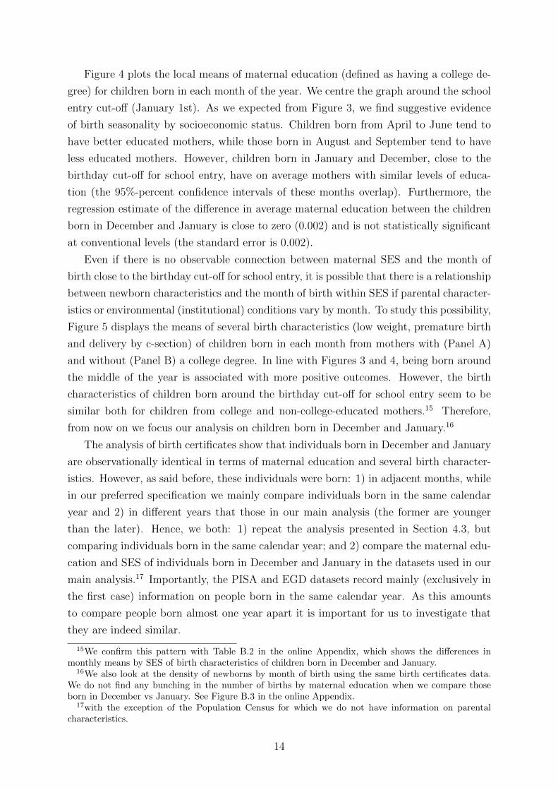
Figure 4 plots the local means of maternal education (defined as having a college de-

gree) for children born in each month of the year. We centre the graph around the school

entry cut-off (January 1st). As we expected from Figure 3, we find suggestive evidence

of birth seasonality by socioeconomic status. Children born from April to June tend to

have better educated mothers, while those born in August and September tend to have

less educated mothers. However, children born in January and December, close to the

birthday cut-off for school entry, have on average mothers with similar levels of educa-

tion (the 95%-percent confidence intervals of these months overlap). Furthermore, the

regression estimate of the difference in average maternal education between the children

born in December and January is close to zero (0.002) and is not statistically significant

at conventional levels (the standard error is 0.002).

Even if there is no observable connection between maternal SES and the month of

birth close to the birthday cut-off for school entry, it is possible that there is a relationship

between newborn characteristics and the month of birth within SES if parental character-

istics or environmental (institutional) conditions vary by month. To study this possibility,

Figure 5 displays the means of several birth characteristics (low weight, premature birth

and delivery by c-section) of children born in each month from mothers with (Panel A)

and without (Panel B) a college degree. In line with Figures 3 and 4, being born around

the middle of the year is associated with more positive outcomes. However, the birth

characteristics of children born around the birthday cut-off for school entry seem to be

similar both for children from college and non-college-educated mothers.15 Therefore,

from now on we focus our analysis on children born in December and January.16

The analysis of birth certificates show that individuals born in December and January

are observationally identical in terms of maternal education and several birth character-

istics. However, as said before, these individuals were born: 1) in adjacent months, while

in our preferred specification we mainly compare individuals born in the same calendar

year and 2) in different years that those in our main analysis (the former are younger

than the later). Hence, we both: 1) repeat the analysis presented in Section 4.3, but

comparing individuals born in the same calendar year; and 2) compare the maternal edu-

cation and SES of individuals born in December and January in the datasets used in our

main analysis.17 Importantly, the PISA and EGD datasets record mainly (exclusively in

the first case) information on people born in the same calendar year. As this amounts

to compare people born almost one year apart it is important for us to investigate that

they are indeed similar.

15We confirm this pattern with Table B.2 in the online Appendix, which shows the differences inmonthly means by SES of birth characteristics of children born in December and January.

16We also look at the density of newborns by month of birth using the same birth certificates data.We do not find any bunching in the number of births by maternal education when we compare thoseborn in December vs January. See Figure B.3 in the online Appendix.

17with the exception of the Population Census for which we do not have information on parentalcharacteristics.

14

Results are reassuring in both exercises. We do not find statistically significant dif-

ferences between individuals born in January and December in the same calendar year in

the STUS, EGD and PISA datasets (which are those used for both our main analysis, in

the first two cases, and motivation, in the last case). In the birth certificate data, we find

a very small difference, below one percentage point, in maternal education between those

born in January and December in the same calendar year, and no differences in new-born

characteristics within SES. Details are available in Online Appendix, Table B.1.

Figure 5: New-born Characteristics and Month of Birth

A. Children of non-college-educated mothers

Low birth weight

7.5

8

8.5

9

9.5

10

%

Jul Aug Sep Oct Nov Dec Jan Feb Mar Apr May JunMonth of birth

C-Section

22

23

24

25

26

%

Jul Aug Sep Oct Nov Dec Jan Feb Mar Apr May JunMonth of birth

Premature

7

7.5

8

8.5

9

9.5

%

Jul Aug Sep Oct Nov Dec Jan Feb Mar Apr May JunMonth of birth

B. Children of college educated mothers

Low birth weight

6

7

8

9

10

%

Jul Aug Sep Oct Nov Dec Jan Feb Mar Apr May JunMonth of birth

C-Section

23

24

25

26

27

28

%

Jul Aug Sep Oct Nov Dec Jan Feb Mar Apr May JunMonth of birth

Premature

6

7

8

9

%

Jul Aug Sep Oct Nov Dec Jan Feb Mar Apr May JunMonth of birth

Notes: Data from Spanish birth certificates. The sample includes the universe of Spanish babies born from

non-college educated mothers (first three figures) or from college educated mothers (last three figures) in the

period from July 2007 to June 2010 and from July 2011 to June 2014. The figures plot, by month of birth, the

percentage of newborns with a low birth weight, the percentage of babies born by cesarean, and the percentage

of premature babies. The means are represented by dots and 95% confidence intervals are in gray.

4.4 Parental time investment by SES and Age

As said before, our identification strategy would be compromised if the secular rate of

change in parental investment by month of birth (age) or grade is different by SES. To

be more precise, note that, a larger increase in time investment from high-SES parents

in reaction to the age at school entry penalty is observationally equivalent to a secular

15

pattern in which parents decrease their time investment as their children grow older

and such decrease is steeper among low-SES families. Hence, we investigate potential

differences in parental investment profiles by age and SES, using data from the Spanish

Time Use Survey (STUS).

Figure B.4 in the online Appendix shows the average time (in minutes per day) that

parents spend helping their children with academic activities by children’s age and SES.

As it is possible to observe, high-SES parents spend on average more time teaching their

school-age children no matter their child’s age. However, and this is the most important

feature for us, the evolution of parental time investment by age is similar for parents from

high- and low-SES: in both cases it tends to increase during the first years of primary

school, reach a peak around age 9 and then go down. This piece of evidence supports

our identification assumption that differences in parental investment by SES and month

of birth in individuals from a same birth cohort are not explained for differences by SES

in parental investments along the life-cycle.

5 The Effect of Being the Youngest

In this section, we present the reduced-form effects of age at school entry on student

and adult outcomes. Our main specification only includes individuals born in January or

December to avoid problems related to birth seasonality in children and maternal char-

acteristics. First, we examine the average effects on medium- and long-term outcomes,

using data from PISA and Spanish population census, respectively. Then, in Subsection

5.2, we analyze whether these effects vary by socioeconomic status.

5.1 Poor Little Children: Short and Long-Term Effects of Being

the Youngest

Columns 1-3 in Table 1 present the results of regressing several measures of school per-

formance (grade retention, maths and reading test scores) on an indicator of whether

the student was born in December or in January, an indicator for being a female and an

indicator for coming from a family with a high socioeconomic status (in the top 25% of

the distribution of the SES index). All the regressions include vectors of dummies for

the year of birth and the PISA survey year. Remember that the oldest children in a

class are born in January (Y oung = 0) and the youngest children are born in December

(Y oung = 1).

Along the same line as the visual evidence, younger students do worse in school than

their older peers. The youngest children in their cohort are 10 percentage points more

likely to have repeated a grade at age 15 than the oldest children (Column 1). This gap

is similar to the gender gap in grade retention (see row 2, also in Column 1), and around

2/5 of the estimated gap for socioeconomic status (see row 3). In the same fashion, there

16

is a clear age gap in student achievement as measured by standardized test scores. On

average, the youngest students have lower test scores in mathematics (-0.14 SD) and in

reading (-0.11 SD). All the results discussed are statistically significant at the one percent

level.

Table 1: Medium- and long-term outcomes

Medium-term outcomes Long-term outcomes

Grade Maths Reading College Employed Partner has

retention score score graduate college degree

(1) (2) (3) (4) (5) (6)

Young 0.105*** -13.861*** -11.164*** -0.00599*** 0.00152 -0.00729***

(0.014) (2.476) (2.370) (0.00198) (0.00247) (0.00216)

Female -0.086*** -11.568*** 34.421*** 0.0281*** -0.125*** -0.00791***

(0.014) (2.464) (2.496) (0.00195) (0.00243) (0.00211)

Top 25% SES -0.259*** 59.506*** 53.436***

(0.015) (2.797) (2.763)

Mean 0.28 499.25 491.24 0.143 0.680 0.119

Observations 12,311 12,311 12,311 226,454 226,454 162,920

Notes: The data analysed in columns 1 to 3 come from Spanish students aged 15 assessed in PISA

2003, 2006, 2009 and 2012. In these first three columns the outcome variables are indicators of school

performance. Grade retention (Column 1) indicates whether the student repeated a grade at least once,

and maths and reading scores (columns 2 and 3) represent the student’s performance in the PISA tests.

The data analysed in columns 4 to 6 come from the 2011 Spanish population census. In Column 4,

the outcome variable is an indicator of whether the individual is a college graduate, in Column 5 it is

an indicator of whether s/he is employed, and in Column 6 an indicator of whether her/his spouse is a

college graduate. The sample includes Spanish individuals born in December and January. “Young” is

an indicator variable that equals one if the student was born in December and equals zero if s/he was

born in January. The regressions presented in columns 1 to 3 include survey year dummies and those

presented in columns 4 to 6 include cohort dummies, where the cohorts are defined as being born from

July to June of the following year. Robust standard errors are in parentheses (clustered at school level

in the case of columns 1 to 3). * p<0.10, ** p<0.05, *** p<0.01.

Columns 4-6, also in Table 1, present the results for the long-term effects of being

an early entrant to school using data from the Spanish population census. The sample

analysed includes individuals born in December and January. We do not include infor-

mation on parental SES because we do not observe this information in the census data.

All the regressions include birth cohort dummies. Note that the birth cohorts here are

defined to compare individuals born in adjacent months (we cannot do this for the PISA

data because we would compare students in different grades). We find that people born

in January (the oldest at school entry) are more likely to have a college degree (by 0.6

percentage points) and to have a more educated partner (one with a college degree, by 0.7

percentage points) than people born in December (the youngest at school entry). Both

17

results are statistically significant at the 1 one percent level. We do not find statistically

significant differences in the probability of being employed. Summing up, Table 1 docu-

ments that – in line with the international literature - people who are younger at school

entry tend to have worse student outcomes, which seems to translate into the long term.

We now move on to analyse differences by parental SES.

5.2 Socioeconomic Status and the Disadvantages of Being Younger:

Poor (Poor) Little Children

Table 2 shows the results of regressing measures of student performance on an indicator

of whether the student was born in December or January, an indicator for being a female,

an indicator for coming from a family in the top 25% of the distribution of the SES index,

and an interaction term between these two indicators (Y oung ∗ top 25% ).

We find clear differences in the effect of age at school entry by socioeconomic back-

ground. Being young is significantly worse for the poor. Young students from a low

socioeconomic background are 12.7 percentage points more likely to have repeated a

grade at age 15 than older students from the same socioeconomic background (see row 1

in Column 1). Importantly, this age effect is significantly smaller for children with a high

socioeconomic background, by 8.7 percentage points (see Row 4). A qualitatively similar

argument can be made about achievement at age 15, as measured by test scores in maths

and reading. Young students from a low socioeconomic background have -0.16 SD (-0.14

SD) lower maths (reading) test scores than their older counterparts (see Row 1, Columns

2-3), while this age effect is significantly smaller for privileged children: 0.1 SD in both

subjects. These results are statistically significant at the one percent level. Still, young

children from high socio-economic status are more likely to have repeated a grade (by 4

percentage points) and have lower math test scores (by 0.06 SD) at age 15 than older

students from the same socioeconomic background (see Row 6-7, Columns 1-2), though

they have statistically similar reading test scores (Row 7, Column 3). Overall, we find

similar results when using the Index of SES as a continuous variable. See Figure B.1 in

the online Appendix.

Therefore, families with a high socioeconomic status seem to buffer the negative effect

of being relatively young on their children’s outcomes, while those with a lower socioeco-

nomic background do not. In Section 6 we discuss two potential mechanisms behind this

result and analyse data on parental involvement in their children’s education to study

whether parents respond differently to age at school entry depending on their SES.

18

Table 2: School performance, entry age and socioeconomic status

Grade retention Maths score Reading score(1) (2) (3)

Young 0.127*** -16.439*** -13.754***(0.018) (2.983) (2.842)

Female -0.086*** -11.553*** 34.435***(0.014) (2.460) (2.493)

Top 25% SES -0.215*** 54.408*** 48.317***(0.019) (3.789) (3.778)

Young * top 25% SES -0.087*** 10.153*** 10.195***(0.028) (5.378) (5.187)

Mean 0.28 499.25 491.24β1 + β3 0.04 -6.29 -3.56p-value: β1 + β3 = 0 0.014 0.028 0.21

Observations 12,311 12,311 12,311

Notes: Data from Spanish students aged 15 assessed in PISA 2003, 2006, 2009 and2012. The outcome variables are indicators of school performance. Grade retention(Column 1) indicates whether the student repeated a grade at least once, and mathsand reading scores (columns 2 and 3) represent the student’s performance in the PISAtests. “Young” (β1) is an indicator variable that equals one if the student was born inDecember and equals zero if s/he was born in January. Young * top 25 SES (β3) is anindicator of the interaction between the variable “Young” and an indicator for comingfrom a family in the top 25% of the distribution of the SES index. All regressions in-clude year dummies as controls. Standard errors clustered at the school level are inparentheses. * p<0.10, ** p<0.05, *** p<0.01.

6 Parental Responses

Two channels could explain why entry age effects are greater among children from low-

SES families. First, high-SES children might actually be ready to start school irrespective

of their age. Note that high-SES children are likely to be more ready to start school than

low-SES children, because of the well-established correlation between family SES and pre-

school investment. This explanation implies that what puts young children at a learning

disadvantage is being below a minimum level of achievement (maturity) on the first day

of school and that growing up in a more nurturing environment makes it more likely that

even the youngest children are above this minimum level.

Second, high-SES parents might increase their investment when their children are

among the youngest at school entry to compensate for their learning disadvantage. Par-

ents with higher SES are likely to be more prepared in terms of financial resources,

human capital and information to invest in their children in reaction to a negative shock.

A dominance of channel one implies that among high-SES families one should not observe

differences in parental investment according to the child’s age at school entry. A domi-

19

nance of channel two implies the opposite. In this section, we analyze data on parental

involvement in their children’s education to study whether parents respond differently to

age at school entry depending on their SES.

We begin the study of parental time investment by using data from the Spanish Time

Use Survey (STUS) and the General Diagnostic Assessment survey (GDA). Then, using

the second of these surveys, we analyze whether parents choose schools with different

inputs when their children are younger at school entry. Finally, we investigate whether

parental responses vary according to the age and the gender of children.

6.1 Parental Time Investment

Our main estimates on parental time investment come from data from the two waves of the

Spanish time use surveys. The STUS reports detailed use of the time that parents spend

participating in activities directly related to their children’s human capital development.

Table 3 reports the estimated coefficients from Equation 1 using as outcomes measures

of the time (in minutes) that parents spend teaching their children, reading and playing

with them, and on other childcare activities. These coefficients represent the effects of

age at school entrance on parental time investments and how such effects interact with

family socioeconomic status (i.e. whether the mother has a college education or not).

Table 3: Parental Time investment

(1) (2) (3)Teaching Read and Play Other childcare

Youngest -0.228 0.644 -4.367(1.156) (2.349) (4.967)

College mother 0.531 6.402* 13.17*(1.481) (3.394) (7.222)

Youngest X College mother 5.233** -1.686 -5.322(2.553) (4.415) (9.659)

Girl 0.476 -1.345 -5.739(1.035) (1.995) (4.104)

Mean 7.55 22.64 85.74β1 + β3 5.01 -1.04 -9.69p-value: β1 + β3 = 0 0.03 0.78 0.24Observations 2,196 2,196 2,196

Notes: Data from the Spanish Time Use Survey 2003 and 2009. The sample consists ofchildren aged 0 to 17 born in December or January in Spain. The outcome variables in-dicate the minutes parents spent daily with their children doing different activities: onesrelated to teaching (Column 1), reading and playing (Column 2), and other childcare ac-tivities (Column 3). “Young” (β1) is an indicator variable that equals one if the studentwas born in December and equals zero if she was born in January. The variable “Collegemother” takes value 1 if the mother of the student has more than secondary educationand zero otherwise. Young X College mother (β3) is an indicator variable of the interac-tion between “Young” and “College mother”. All the reported models include a vector ofdummies for year of birth, and day of week and quarter of interview. Standard errors areclustered at the household level. *** p<0.01, ** p<0.05, * p<0.1

20

In households with non-college-educated mothers, the school entry age does not seem

to affect parental time investment in activities related to children’s human capital devel-

opment. The coefficient for being the youngest in the three regressions presented has a

small magnitude and is not statistically significant at conventional levels. In contrast,

households with university-educated mothers do spend significantly more time with their

children on activities related to teaching (+ 5 minutes per day, significant at the five

percent level) than their older peers from similar types of families. This is a large effect.

In context, parents in our sample spend on average 7.5 minutes per day helping their

children with school activities. There are not statistically significant differences accord-

ing to children’s month of birth in the time that highly educated parents spend on the

other childcare activities. Thus, more educated parents compensate by investing more

time in teaching activities when their children are among the youngest in their school

cohort. Interestingly, this effect seems to be larger during the school months (estimate is

7 minutes, see Table B.4 in the online Appendix).

We complement these results with data from the General Diagnostic Assessment sur-

vey. Here, using self-reported statements, we analyze whether parents respond to school

entry age by changing their behaviour regarding helping children with their homework,

checking their homework, or by attending school meetings more frequently (as reported

by the students). As before, we examine whether the parental responses depend on

maternal education.

Table 4: Parental Involvement

(1) (2) (3)Help with homework Parents check homework Parents go to school meetings

Young 0.00447 0.00354 -0.0228(0.0154) (0.0190) (0.0201)

College mother 0.0349∗ -0.108∗∗∗ -0.0267(0.0192) (0.0271) (0.0275)

Young X College mother 0.0750∗∗∗ 0.0724∗∗ 0.0425(0.0247) (0.0364) (0.0377)

Girl -0.0152 0.0327∗∗ -0.00897(0.0123) (0.0166) (0.0169)

Mean 0.85 0.69 0.59β1 + β3 0.079 0.076 0.02p-value: β1 + β3 = 0 0.00 0.02 0.54

Observations 3461 3350 3345

Notes: The data comes from the General Diagnostic Assessment survey of 2009. The sample includes Spanish students enrolledin 4th grade who were born in December or in January. The outcome variables are different measures of parental involvementin children’s education: a variable indicating whether parents help their children with the homework (Column 1), an indicatorvariable of parents checking children’s homework (Column 2), and a variable indicating whether parents frequently go to schoolmeetings (Column 3). “Young” (β1) is an indicator variable that equals one if the student was born in December and equals zeroif she was born in January. The variable “College mother” takes value 1 if the mother of the student has a college education andzero otherwise. Young X College mother (β3) is an indicator variable of the interaction between “Young” and “College mother”.Standard errors are clustered at the school level. * p<0.10, ** p<0.05, *** p<0.01

Table 4 presents the estimated coefficients from Equation 1 in which the outcome

variables are indicators of different dimensions of parental involvement. As in the time use

21

data, we do not find that households with non-college educated mothers invest differently

if their children enter school at a younger age (first row of Column 1); and, we do

find differences in households with college-educated mothers. Children from university-

educated mothers are significantly more likely to receive help to do their homework (+

8 percentage points, significant at the 1 percent level) and to have their parents check

their homework (+7.6 percentage points, significant at the five percent level) than their

older peers from similar types of family (see Rows 6-7 in Columns 1-2). We do not find

more likely though that their parents go to school meetings (Column 3). Summing up,

this evidence shows that more educated parents compensate for school disadvantage by

putting more effort into helping their children with their with academic tasks.18

6.2 School Choice

We now analyse whether parents respond to school entry age by sending their children

to schools with different levels of inputs, and whether these reactions vary according to

the level of maternal education.

Using the General Diagnostic Assessment, we look at differences in several school

inputs between the schools that students born in December and January attend. To do

this, we rely on the principal and teacher survey questionnaires. Table 5 presents the

coefficient estimates from Equation 1. In the first column, the outcome is an indicator

variable of whether the student attends a concertada school: a privately-managed school,

which may offer a more customized education environment than regular schools.19 We do

not find that entry age significantly affects school choice regarding this specific feature, in-

dependently of the mother’s education. However, younger children with college-educated

mothers are more likely to attend schools with better teachers (+ 0.09 SD in a teacher

quality index significant at the one percent level) and with parents more involved in the

school (+ 0.088 SD in a parental involvement index, significant at the five percent level)

than their older peers from similar types of families (Row 6, Columns 4-5). In contrast,

we do not observe significant differences in the characteristics of the schools attended by

children from mothers without a college education (see the first row in Columns 1-5). In

the online Appendix we provide the disaggregated effects of the variables that constitute

the Teacher Quality and the Parental Involvement indexes, plus a School Quality Index,

which aggregates the nine variables analysed (which shows results consistent with those

presented in Table 5). It is also worth to notice that we find effects in both variables

reported by teachers (Parental Involvement Index) and principals (Teacher Quality). The

principals assesments refer to overall teacher quality at the school level, not the teacher

18We also compare individuals born in adjacents January and December months and find similarresults, available in Online Appendix, Table B.3.

19According to figures from Eurostat for Spain, 68% of primary school students attend public schools,28% concertada schools and 4% fully private schools.

22

in the specific classroom that the child attends. This is relevant because supports the ar-

gument that high-SES parents choose schools with better inputs when their children are

the youngest at school entry–in contrast to an alternative explanation in which younger

high-SES children are sorted into better classrooms either because in general high-SES

children attend more responsive schools or because parents lobby for better classrooms

rather than choosing better schools. Therefore, we find evidence that more educated

parents are more likely to send their children to schools with better inputs when they

enter school at an earlier age.20

Table 5: School Quality

(1) (2) (3) (4) (5)Concertada Class Peers motivated Teacher Parental

school size to learn quality index involvement index

Young 0.00284 0.214 -0.0256 -0.00598 -0.00791(0.0204) (0.179) (0.0214) (0.0244) (0.0304)

College mother 0.232*** 1.325*** 0.138*** 0.00358 -0.00558(0.0299) (0.289) (0.0271) (0.0319) (0.0417)

Young X College mother 0.0361 -0.576* 0.0669** 0.0984** 0.0960**(0.0370) (0.338) (0.0332) (0.0431) (0.0485)

Girl 0.0164 0.136 -0.00876 0.00822 0.00959(0.0170) (0.141) (0.0161) (0.0203) (0.0221)

Mean 0.40 23.89 0.69 0.01 0.02β1 + β3 0.039 -0.362 0.041 0.092 0.088p-value: β1 + β3 = 0 0.23 0.19 0.13 0.01 0.04

Observations 3171 3171 3171 3171 3171

Notes: The data come from the General Diagnostic Assessment survey 2009. The sample includes Spanish students enrolledin grade 4 who were born in December or January. The outcome variables are different school characteristics: a concertadaschool indicator (Column 1), class size (Column 2), an indicator of whether the teacher reports that the students in her classare very motivated (Column 3), a Teacher Quality Index (Column 4) and a Parental Involvement Index (Column 5) “Young”(β1) is an indicator variable that equals one if the student was born in December and equals zero if she was born in January.The variable “College mother” takes value 1 if the mother of the student has a college education and zero otherwise. YoungX College mother (β3) is an indicator variable of the interaction between “Young” and “College mother”. Standard errorsare clustered at the school level. * p<0.10, ** p<0.05, *** p<0.01

Overall, these results are consistent with the idea that more educated parents com-

pensate when their children start school at an earlier age by spending more time helping

their children with school and sending their children to schools with better inputs. Along

the same lines, we do not find that less educated parents change their patterns of in-

vestment in their children to compensate for or reinforce the effects of entry age. This

socioeconomic difference in compensating behaviour helps to explain why the detrimental

effect of being young at school entry is greater for low-SES children.

20Also in the General Diagnostic Assessment, both parents and students declare (in separate surveys)if the student is enrolled in her current school because she lives in the school’s catchment area. We usethis information as an indicator that parents choose (or not) to send their young children to differentschools from the default option. We find that children from mothers without a college education seemto go to their neighborhood school regardless of the month when they were born, while young childrenfrom college-educated mothers seem to be more likely to attend a different school to the default optionthan the older children from similarly educated mothers. Table B.6 in the online Appendix reports theresults.

23

6.3 Heterogeneity Analysis

6.3.1 Parental Time Investment according to Age

Using data from the Time Use survey, Table 6 reports the estimated coefficients from

Equation 1 for three age groups: children younger than 6 (who are below school age at

the moment of the survey), children aged 6 to 12 (who are of primary school age), and

children aged 13 to 17 (who are of secondary school age). Table 3 shows that young

children with highly educated mothers spend more time with their parents on activities

related to teaching than their older peers. If these results are driven by a mere age effect

and not by what is going on in school (i.e. not by a negative early entry age effect), we

might expect a similar pattern if we analyse the sample of children who are outside of

compulsory school age. However, as shown in Table 6 (row 6 in columns 1–3), the sum of

the coefficients for Young and the interaction Young*College Mother is not significantly

different from zero when estimated using the sample of children aged 0 to 5. This includes

both parental time related to teaching and all other childcare. In contrast, the coefficient

for this interaction in the teaching time regression is positive and statistically significant

when we analyse the sample of children who are above school entry age, i.e. aged 6 to 12

(Column 4) and 13 to 17 (Column 7).

Interestingly, the magnitude of the point estimate in the sample of children aged 6 to

12 seems to be larger than that in the sample of children aged 13 to 17. While in the former

sample the youngest children from households with university-educated mothers spend

10 minutes more a day with their parents on activities related to teaching than their older

peers, in the latter sample the corresponding figure amounts to only 7 minutes (and it is,

marginally, insignificant). This pattern is consistent with the ideas that 1) parents react

to their realization that their child has a school disadvantage, and 2) that the returns on

investments at earlier ages are larger. This is only suggestive evidence as we do not have

enough statistical precision to rule out that both parameters are of the same magnitude.

As Table B.5 in the online Appendix shows, the compensating effect becomes larger when

we exclude the summer months (point estimate is 15 minutes), which reinforces the idea

that parental reactions are driven by what is going on in school. Once more, across the

three age groups we observe that in households with more lowly educated mothers entry

age does not seem to affect parental time investment in activities related to children’s

human capital development.

24

Table 6: Parental Time Investment by Age Groups

(1) (2) (3) (4) (5) (6) (7) (8) (9)Teaching Reading and Playing Other childcare Teaching Reading and Playing Other childcare Teaching Reading and Playing Other childcare

0-5 6-12 13-17Young 0.218 3.605 -14.61 -1.251 -2.315 6.001 -1.273 2.089 -3.802

(1.648) (7.309) (13.93) (2.324) (3.489) (7.043) (1.674) (1.807) (4.115)College mother 1.778 11.64 27.40* -1.179 7.295* 14.12 0.553 -0.348 -4.407

(2.145) (7.376) (14.47) (3.021) (4.231) (9.656) (2.102) (1.676) (4.193)Young X College Mother -1.779 -8.791 -10.46 11.38** 2.436 -9.200 6.292 0.0527 9.137

(3.092) (10.39) (21.03) (5.118) (5.955) (12.57) (4.836) (3.327) (6.026)Girl 0.924 -3.036 -13.75 -0.462 0.486 -3.465 0.991 -3.430** -4.585

(1.444) (4.942) (9.388) (1.936) (2.730) (5.752) (1.522) (1.704) (3.513)

Mean 4.77 45.56 171.24 12.54 16.42 63.99 4.44 3.89 13.95β1 + β3 -1.56 -5.19 -25.07 10.13 0.12 -3.20 5.02 2.14 5.34t-test β1 + β3 = 0 0.54 0.49 0.13 0.03 0.98 0.76 0.27 0.44 0.25Observations 744 744 744 812 812 812 640 640 640

Notes: Data from the Spanish Time Use Survey 2003 and 2009. The sample is of children aged 0 to 17 born in December or January in Spain. The first 3 columns include only children younger than 6, columns 4 to 6include children aged 6 to 12 and the last 3 columns include children aged 13 to 17. The outcome variables indicate the minutes a day parents spent with their children doing different activities: ones related to teaching,to reading and playing, and other childcare activities. “Young” (β1) is an indicator variable that equals one if the student was born in December and equals zero if she was born in January. The variable “College mother”takes value 1 if the mother of the student has more than secondary education and zero otherwise. Young X College mother (β3) is an indicator variable of the interaction between “Young” and “College mother”. All thereported models include a vector of dummies for year of birth, and day of week and quarter of interview.. Standard errors are clustered at the household level. *** p<0.01, ** p<0.05, * p<0.1

25

6.3.2 Gender Differences

Finally, we analyse whether the responses from highly- and poorly-educated parents vary

according to the student’s gender. We look at gender gaps motivated by the literatures

that show that girls mature faster than boys (see a discussion in Bertrand and Pan,

2013), and that boys strugle more when they face disadvantaged environments (see for

example in the literature on family structure: Figlio et al., 2016; Fan et al., 2015). To

do this, we first analyze whether the age effect on student outcomes, as measured by

PISA, differs with gender. We find some evidence, which is reported in Table 7, that

this is the case. As before, we observe that being among the youngest at school entry

has a significant negative effect among children from low-SES families, both for boys

and girls (see row 1, columns 1-6). However, the story seems to be different for children

from high-SES families. On the one hand, boys from high-SES families do not seem to

manage to overcome the age disadvantage (see rows 5 and 6, Columns 1-3). Compared

to their older peers, young boys from high-SES are more likely to have repeated a grade

(by 7.4 percentage points, with statistical significance at the one percent level) and to

have lower test scores in math (by 0.11 SD, with statistical significance at the one percent

level) and reading (by 0.08 SD, with statistical significance at the ten percent level) at

age 15. In contrast, we do not observe a gap in student outcomes among high-SES girls

(Columns 4-6). The magnitude of the coefficients reported in Row 5 is small and none is

statistically significant at conventional levels (see Row 6). Therefore, at age 15, there are

no differences in academic performance between December- and January-born girls who

come from advantaged families.

Table 7: School Performance by Student Gender

Boys Girls

(1) (2) (3) (4) (5) (6)Grade retention Math score Reading score Grade retention Math score Reading score

Young 0.135*** -17.197*** -16.526*** 0.118*** -15.686*** -11.031***(0.014) (2.448) (2.492) (0.026) (4.209) (4.052)

Top 25% SES -0.231*** 55.298*** 50.989*** -0.198*** 53.294*** 45.409***(0.019) (3.395) (3.456) (0.026) (4.952) (4.579)

Young * top 25% SES -0.061** 6.599 8.930* -0.115*** 14.187* 11.777*(0.027) (4.790) (4.877) (0.035) (7.330) (6.630)

Mean 0.33 505.08 473.92 0.23 493.58 508.09β1 + β3 0.07 -10.60 -7.60 0.003 -1.50 0.75p-value: β1 + β3 = 0 0.002 0.01 0.07 0.90 0.81 0.89Observations 6070 6070 6070 6241 6241 6241

Notes: Data from Spanish students aged 15 assessed in PISA 2003, 2006, 2009 and 2012. The first 3 columns correspond to the analysis of thesample of boys and the last 3 to the sample of girls. The outcome variables are indicators of school performance. Grade retention (Column1) indicates whether the student repeated a grade at least once, and maths and reading scores (column 2 and 3) represent the performance ofthe student in the PISA tests. “Young” (β1) is an indicator variable that equals one if the student was born in December and zero if she wasborn in January. Young * top 25 SES (β3) is an indicator of the interaction between the variable “Young” and an indicator for coming froma family in the top 25% of the distribution of the SES index. All regressions include year dummies as controls. Standard errors clustered atschool level are in parentheses. * p<0.10, ** p<0.05, *** p<0.01

We use data from the General Diagnostic Assessment to study differences in parental

investments by SES and gender because this data has a larger sample size than the

26

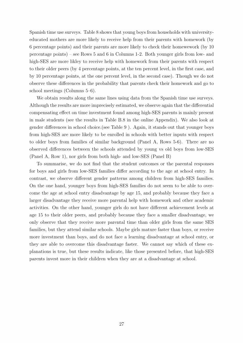
Spanish time use surveys. Table 8 shows that young boys from households with university-

educated mothers are more likely to receive help from their parents with homework (by

6 percentage points) and their parents are more likely to check their homewework (by 10

percentage points) – see Rows 5 and 6 in Columns 1-2. Both younger girls from low- and

high-SES are more likley to receive help with homework from their parents with respect

to their older peers (by 4 percentage points, at the ten percent level, in the first case, and

by 10 percentage points, at the one percent level, in the second case). Though we do not

observe these differences in the probability that parents check their homework and go to

school meetings (Columns 5–6).

We obtain results along the same lines using data from the Spanish time use surveys.

Although the results are more imprecisely estimated, we observe again that the differential

compensating effect on time investment found among high-SES parents is mainly present

in male students (see the results in Table B.8 in the online Appendix). We also look at

gender differences in school choice.(see Table 9 ). Again, it stands out that younger boys

from high-SES are more likely to be enrolled in schools with better inputs with respect

to older boys from families of similar background (Panel A, Rows 5-6). There are no

observed differences between the schools attended by young vs old boys from low-SES

(Panel A, Row 1), nor girls from both high- and low-SES (Panel B)

To summarise, we do not find that the student outcomes or the parental responses

for boys and girls from low-SES families differ according to the age at school entry. In

contrast, we observe different gender patterns among children from high-SES families.

On the one hand, younger boys from high-SES families do not seem to be able to over-

come the age at school entry disadvantage by age 15, and probably because they face a

larger disadvantage they receive more parental help with homework and other academic

activities. On the other hand, younger girls do not have different achievement levels at

age 15 to their older peers, and probably because they face a smaller disadvantage, we

only observe that they receive more parental time than older girls from the same SES

families, but they attend similar schools. Maybe girls mature faster than boys, or receive

more investment than boys, and do not face a learning disadvantage at school entry, or

they are able to overcome this disadvantage faster. We cannot say which of these ex-

planations is true, but these results indicate, like those presented before, that high-SES

parents invest more in their children when they are at a disadvantage at school.

27

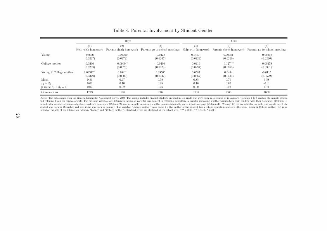
Table 8: Parental Involvement by Student Gender

Boys Girls

(1) (2) (3) (4) (5) (6)Help with homework Parents check homework Parents go to school meetings Help with homework Parents check homework Parents go to school meetings

Young -0.0324 -0.00399 -0.0428 0.0407∗ 0.00981 -0.00318(0.0227) (0.0279) (0.0267) (0.0224) (0.0260) (0.0296)

College mother 0.0266 -0.0909∗∗ -0.0460 0.0419 -0.127∗∗∗ -0.00478(0.0239) (0.0376) (0.0378) (0.0297) (0.0383) (0.0391)

Young X College mother 0.0934∗∗∗ 0.104∗∗ 0.0950∗ 0.0587 0.0444 -0.0115(0.0329) (0.0509) (0.0537) (0.0367) (0.0515) (0.0522)

Mean 0.86 0.67 0.59 0.85 0.70 0.58β1 + β3 0.06 0.10 0.05 0.10 0.05 -0.01p-value β1 + β3 = 0 0.02 0.02 0.26 0.00 0.23 0.74

Observations 1743 1687 1687 1718 1663 1658

Notes: The data comes from the General Diagnostic Assessment survey 2009. The sample includes Spanish students enrolled in 4th grade who were born in December or in January. Columns 1 to 3 analyse the sample of boysand columns 4 to 6 the sample of girls. The outcome variables are different measures of parental involvement in children’s education: a variable indicating whether parents help their children with their homework (Column 1),an indicator variable of parents checking children’s homework (Column 2), and a variable indicating whether parents frequently go to school meetings (Column 3). “Young” (β1) is an indicator variable that equals one if thestudent was born in December and zero if she was born in January. The variable “College mother” takes value 1 if the mother of the student has a college education and zero otherwise. Young X College mother (β3) is anindicator variable of the interaction between “Young” and “College mother”. Standard errors are clustered at the school level. *** p<0.01, ** p<0.05, * p<0.1

28

Table 9: School Choice by Student Gender

Panel A: Boys

(1) (2) (3) (4) (5)Concertada school Class size Peers motivated to learn Teacher quality index Parental involvement index

Young 0.00366 0.314 -0.0309 0.0228 0.00871(0.0278) (0.255) (0.0307) (0.0361) (0.0441)

College mother 0.192∗∗∗ 1.125∗∗∗ 0.114∗∗∗ -0.00227 -0.0315(0.0391) (0.413) (0.0364) (0.0466) (0.0589)

Young X College mother 0.0967∗ -0.671 0.0911∗ 0.0838 0.114(0.0510) (0.479) (0.0481) (0.0630) (0.0718)

Mean 0.40 23.85 0.69 0.00 0.01β1 + β3 0.10 -0.36 0.06 0.11 0.12p-value: β1 + β3 = 0 0.02 0.40 0.11 0.04 0.04

Observations 1596 1596 1596 1596 1596

Panel B: Girls

(1) (2) (3) (4) (5)Concertada school Class size Peers motivated to learn Teacher quality index Parental involvement index

Young 0.00230 0.123 -0.0202 -0.0340 -0.0239(0.0284) (0.274) (0.0303) (0.0344) (0.0396)

College mother 0.279∗∗∗ 1.559∗∗∗ 0.166∗∗∗ 0.0122 0.0257(0.0411) (0.288) (0.0363) (0.0458) (0.0520)

Young X College mother -0.0301 -0.533 0.0392 0.109∗ 0.0719(0.0532) (0.424) (0.0476) (0.0629) (0.0656)

Mean 0.41 23.94 0.68 0.01 0.02β1 + β3 -0.03 -0.41 0.02 0.08 0.05p-value: β1 + β3 = 0 0.55 0.15 0.61 0.14 0.42

Observations 1575 1575 1575 1575 1575

Notes: The data come from the General Diagnostic Assessment survey 2009. The sample includes Spanish students enrolled in 4th grade who were born in Decemberor January. Panel A analyses the sample of boys and Panel B the sample of girls. The outcome variables are different school characteristics: a concertada schoolindicator (Column 1), class size (Column 2), an indicator of whether the teacher reports that the students in her class are very motivated (Column 3), a TeacherQuality Index (Column 4) and a Parental Involvement Index (Column 5). “Young” (β1) is an indicator variable that equals one if the student was born in Decemberand zero if she was born in January. The variable “College mother” takes value 1 if the mother of the student has a college education and zero otherwise. Young XCollege mother (β3) is an indicator variable of the interaction between “Young” and “College mother”. All reported models include a vector of dummies for birthcohort. Standard errors are clustered at the school level. *** p<0.01, ** p<0.05, * p<0.1

29

7 Conclusions

To understand inequality in human capital it is necessary to understand how parental

investment varies according to socioeconomic status. Our results contribute to this goal

by providing evidence on how parents can react to a widely-used school policy that puts

younger children at a learning disadvantage. They are consistent with the idea that

parental responses vary with socioeconomic status.

Highly-educated parents compensate when their children enter school at an earlier

age by spending more time helping their children with learning activities and choosing

schools with better inputs for them, when their children enter school at an earlier age. We

do not find a similar pattern among less educated parents. This socioeconomic difference

in behavior can potentially explain why the disadvantage of being young at school entry

is greater for children from disadvantaged backgrounds. Interestingly, the response of

highly educated parents is particularly present in the case of boys.

There is a well-established empirical relationship between parental socioeconomic sta-

tus and student (and longer-term) outcomes. Differences in planned investment paths are

likely to play a key role in this. Our results highlight an additional channel: differences

in investment due to different responses according to parental background to policies (or

potentially life shocks) that put children at a learning disadvantage. In other words, we

find evidence that more educated parents are more prepared to handle disadvantage and

can then protect their children from it by increasing the resources they allocate to them.

Our findings call for the design of public policies targeting those who need support

the most: young children from low-SES families, presumably with a focus not only on

the children, but also on parents and schools.

The results presented in this paper are also informative about the effects of teaching

the same curriculum to children with different achievement levels, which is a common

practice across countries. Our findings suggest that the task of dealing with a unique

curriculum from the position of a learning disadvantage can be particularly daunting

for children from low-SES families. Policies aiming to allow schools to teach at the right

level (using some degree of tracking or supplementary activities according to achievement

level) are worth exploring.

References

Albornoz, F., S. Berlinski, and A. Cabrales (2018): “Motivation, resources and

the organization of the school system,” Journal of the European Economic Association.

Almond, D. and B. Mazumder (2013): “Fetal Origins and Parental Responses,”

Annual Review of Economics, 5, 37–56.

Attar, I. and D. Cohen-Zada (2017): “The Effect of School Entrance Age on Edu-

30

cational Outcomes: Evidence Using Multiple Cutoff Dates and Exact Date of Birth,”

Tech. rep., IZA Institute of Labor Economics.

Bedard, K. and E. Dhuey (2006): “The Persistence of Early Childhood Maturity:

International Evidence of Long-Run Age Effects,” The Quarterly Journal of Economics,

121, 1437–1472.

——— (2012): “School-Entry Policies and Skill Accumulation Across Directly and Indi-

rectly Affected Individuals,” Journal of Human Resources, 47, 643–683.

Bertrand, M. and J. Pan (2013): “The trouble with boys: Social influences and the

gender gap in disruptive behavior,” American Economic Journal: Applied Economics,

5, 32–64.

Black, S. E., P. J. Devereux, and K. G. Salvanes (2011): “Too young to leave

the nest? The effects of school starting age,” The Review of Economics and Statistics,

93, 455–467.

Borra, C., L. Gonzalez, and A. Sevilla (2015): “The Impact of Scheduling Birth

Early on Infant Health,” Tech. rep., Barcelona Graduate School of Economics.

Buckles, K. S. and D. M. Hungerman (2013): “Season of birth and later outcomes:

Old questions, new answers,” Review of Economics and Statistics, 95, 711–724.

Calsamiglia, C. (2014): “Matching Practices for Elementary and Secondary Schools -

Spain,” Tech. rep., Matching in Practice.

Calsamiglia, C. and A. Loviglio (2016): “Maturity and school outcomes in an

inflexible system: evidence from Catalonia,” .

Cook, P. J. and S. Kang (2016): “Birthdays, schooling, and crime: regression-

discontinuity analysis of school performance, delinquency, dropout, and crime initi-

ation,” American Economic Journal: Applied Economics, 8, 33–57.

Crawford, C., L. Dearden, and C. Meghir (2007): When you are born matters:

The impact of date of birth on child cognitive outcomes in England, Centre for the

Economics of Education, London School of Economics and Political Science.

Das, J., S. Dercon, J. Habyarimana, P. Krishnan, K. Muralidharan, and

V. Sundararaman (2013): “School inputs, household substitution, and test scores,”

American Economic Journal: Applied Economics, 5, 29–57.

Del Boca, D., C. Flinn, and M. Wiswall (2014): “Household choices and child

development,” The Review of Economic Studies, 81, 137–185.

31

Dhuey, E. (2016): “Age at school entry: How old is old enough?” IZA World of Labor.

Dhuey, E., D. Figlio, K. Karbownik, and J. Roth (2017): “School Starting Age

and Cognitive Development,” Tech. rep., National Bureau of Economic Research.

Dhuey, E. and S. Lipscomb (2008): “What makes a leader? Relative age and high

school leadership,” Economics of Education Review, 27, 173 – 183.

Elder, T. E. (2010): “The importance of relative standards in ADHD diagnoses: Evi-

dence based on exact birth dates,” Journal of Health Economics, 29, 641 – 656.

Elder, T. E. and D. H. Lubotsky (2009): “Kindergarten Entrance Age and Chil-

dren’s Achievement: Impacts of State Policies, Family Background, and Peers,” Journal

of Human Resources, 44, 641–683.

Eurydice (2011): “Grade Retention during Compulsory Education in Europe: Regula-

tions and Statistics,” Tech. rep., Eurydice.

Fan, X., H. Fang, and S. Markussen (2015): “Mothers’ Employment and Children’s

Educational Gender Gap,” NBER Working Papers 21183, National Bureau of Economic

Research, Inc.

Figlio, D., K. Karbownik, J. Roth, M. Wasserman, et al. (2016): “Family

Disadvantage and the Gender Gap in Behavioral and Educational Outcomes,” Tech.

rep., National Bureau of Economic Research.

Fredriksson, P. and B. Ockert (2014): “Life-cycle Effects of Age at School Start,”

The Economic Journal, 124, 977–1004.

Fredriksson, P., B. Ockert, and H. Oosterbeek (2016): “Parental Responses to

Public Investments in Children: Evidence from a Maximum Class Size Rule,” Journal

of Human Resources.

Gratz, M. and F. Bernardi (2017): “Parental Responses to Disadvantageous Life

Events: The Month of Birth Penalty in England,” Social Inequality Across the Gener-

ations: The Role of Compensation and Multiplication in Resource Accumulation, 68.

Grenet, J. (2011): “Academic performance, Educational Trajectories and the Persis-

tence of Date of Birth Effects. Evidence from France,” .

IEA (2011): “TIMSS 2011 Contextual Questionnaires: Curriculum Questionnaire,” Tech.

rep., International Association for the Evaluation of Educational Achievement, ac-

cessed: 2018-04-04.

32

Landersø, R., H. S. Nielsen, and M. Simonsen (2016): “School Starting Age and

the Crime-age Profile,” The Economic Journal, n/a–n/a.

McEwan, P. J. and J. S. Shapiro (2008): “The Benefits of Delayed Primary School

Enrollment: Discontinuity Estimates Using Exact Birth Dates,” Journal of Human

Resources, 43, 1–29.

Muhlenweg, A. M. and P. A. Puhani (2010): “The Evolution of the School-Entry

Age Effect in a School Tracking System,” Journal of Human Resources, 45, 407–438.

Pop-Eleches, C. and M. Urquiola (2013): “Going to a Better School: Effects and

Behavioral Responses,” American Economic Review, 103, 1289–1324.

Schwandt, H. and A. Wuppermann (2016): “The youngest get the pill: ADHD

misdiagnosis in Germany, its regional correlates and international comparison,” Labour

Economics, 43, 72 – 86.

Todd, P. E. and K. I. Wolpin (2003): “On The Specification and Estimation of The

Production Function for Cognitive Achievement,” Economic Journal, 113, F3–F33.

33

Appendix

Tables: Summary Statistics

Table A.1: Spanish Birth Certificates: Summary Statistics

(1) (2)All Dec and Jan

College mother 0.369 0.368(0.483) (0.482)

Mother lives with partner 0.919 0.916(0.273) (0.278)

Spanish mother 0.828 0.825(0.377) (0.380)

Mothers age 32.00 32.03(5.170) (5.209)

Number of children 1.615 1.614(0.783) (0.788)

Born prematurely 0.0778 0.0798(0.268) (0.271)

Cesarean section 0.244 0.245(0.430) (0.430)

Low-birth weight 0.0822 0.0851(0.275) (0.279)

Observations 2,275,737 378,624

Notes: Data from Spanish birth certificates from July 2007 toJune 2014 (except for July 2010-June 2011). Column 1 reportsmeans and standard errors, in parentheses, for the full sample andColumn 2 for those born in December and January.

34

Table A.2: Programme for International Student Assessment: Summary Statistics

(1) (2)All Dec and Jan

Girl 0.501 0.507(0.500) (0.500)

Repeater 0.276 0.280(0.447) (0.449)

Times repeated 0.335 0.344(0.586) (0.597)

Maths 501.2 499.3(83.51) (84.32)

Reading 492.3 491.2(83.64) (84.72)

Observations 74,832 12,311

Notes: Data on Spanish students aged 15 assessedin PISA 2003, 2006, 2009 and 2012. Repeater is anindicator of whether the student repeated a gradeat least once, and maths and reading scores rep-resent the performance of the student in the PISAtests. Column 1 reports means and the standarderrors, in parentheses, for the full sample and Col-umn 2 for those born in December and January.

35

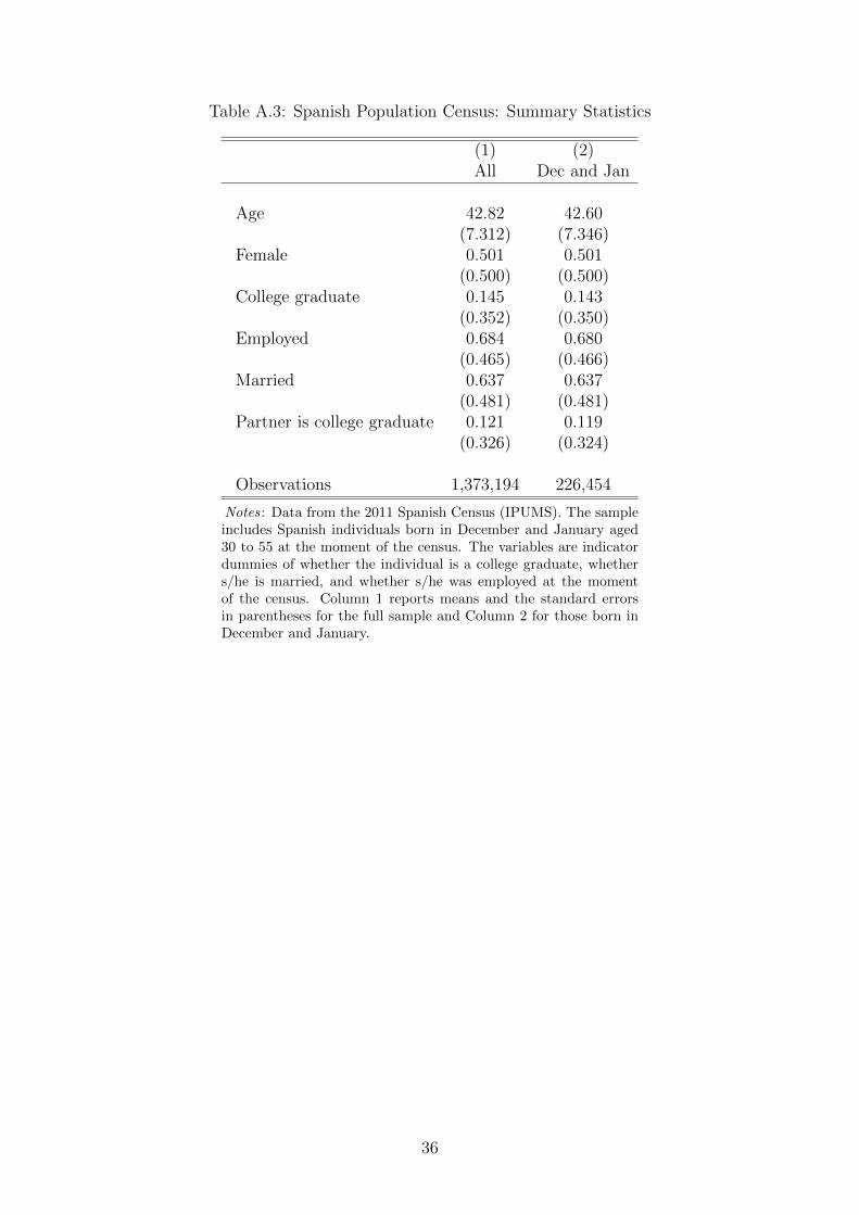
Table A.3: Spanish Population Census: Summary Statistics

(1) (2)All Dec and Jan

Age 42.82 42.60(7.312) (7.346)

Female 0.501 0.501(0.500) (0.500)

College graduate 0.145 0.143(0.352) (0.350)

Employed 0.684 0.680(0.465) (0.466)

Married 0.637 0.637(0.481) (0.481)

Partner is college graduate 0.121 0.119(0.326) (0.324)

Observations 1,373,194 226,454

Notes: Data from the 2011 Spanish Census (IPUMS). The sampleincludes Spanish individuals born in December and January aged30 to 55 at the moment of the census. The variables are indicatordummies of whether the individual is a college graduate, whethers/he is married, and whether s/he was employed at the momentof the census. Column 1 reports means and the standard errorsin parentheses for the full sample and Column 2 for those born inDecember and January.

36

Table A.4: General Diagnostic Assessment: Summary Statistics

(1) (2)All Dec and Jan

Girl 0.499 0.495(0.500) (0.500)

College mother 0.298 0.304(0.457) (0.460)

Help with homework 0.861 0.856(0.346) (0.351)

Parents check homework 0.693 0.687(0.461) (0.464)

Parents go to school meetings 0.579 0.586(0.494) (0.493)

Concertada school 0.396 0.401(0.489) (0.490)

Class size 23.90 23.87(3.901) (4.067)

Peers motivated to learn 0.704 0.691(0.456) (0.462)

Parental interest in learning problems 0.284 0.289(0.451) (0.453)

Parental interest in grades 0.385 0.384(0.487) (0.487)

Parents attend meetings 0.481 0.481(0.500) (0.500)

Teachers continual training 0.791 0.789(0.406) (0.408)

Teachers target students with learning disadvantages 0.604 0.616(0.489) (0.486)

Teachers follow students’ progress daily 0.704 0.706(0.456) (0.456)

Observations 18,583 3,085

Notes: The data comes from the General Diagnostic Assessment survey 2009. The sample in-cludes Spanish students enrolled in 4th grade. The variable “college mother” takes value 1 ifthe mother of the student has a college degree and zero otherwise. “Concertada school” takesvalue 1 if the school is privately managed and is zero otherwise. Class size indicates the num-ber of students in the class. The rest of the variables are indicators about parental involmentin their children education (measured in a student survey) and school inputs (measured in sur-veys to parents and school principals). Column 1 reports means and standard deviations inparentheses for the full sample and Column 2 for those born in December and January.

37

Table A.5: Spanish Time Use Surveys 2003 and 2009: Summary Statistics

(1) (2)All Dec and Jan

Girl 0.484 0.500(0.500) (0.500)

College mother 0.364 0.364(0.481) (0.481)

Time spent teaching 7.690 7.546(25.51) (24.88)

Time spent reading and playing 22.71 22.64(53.28) (51.98)

Childcare time 86.21 85.74(118.9) (118.6)

Observations 13,045 2,196

Notes: Data from the Spanish Time Use Survey 2003 and 2009. Thesample is of children aged 0 to 17 born in Spain. The variable “col-lege mother” takes value 1 if the mother of the student has a collegedegree and zero otherwise. The other variables indicate the minutes aday parents spent with their children doing different activities: onesrelated to teaching, reading and playing, and other childcare activi-ties. Column 1 reports means and standard deviations, in parenthe-ses for the full sample and Column 2 for those born in December andJanuary.

38

Online Appendix

Figure B.1: School Performance at age 15: Young vs. Old According to SES

Repeater

Maths score Reading score

Notes: Data on Spanish students aged 15 assessed in PISA 2003, 2006, 2009 and 2012. For young (born in

December) and old (born in January) students the figures plot the predicted marginal effect of socio-economic

status on: the probability of having repeated at least one grade (top), and the mean test score in maths and

reading at PISA (bottom). Point estimates and 95% confidence intervals.

39

Figure B.2: Birth Characteristics and Month of Birth

All mothersCollege

35

36

37

38

39

%

Jul Aug Sep Oct Nov Dec Jan Feb Mar Apr May JunMonth of birth

Spanish

81

82

83

84

%

Jul Aug Sep Oct Nov Dec Jan Feb Mar Apr May JunMonth of birth

In a couple

90.5

91

91.5

92

92.5

%

Jul Aug Sep Oct Nov Dec Jan Feb Mar Apr May JunMonth of birth

Age

31.8

31.9

32

32.1

32.2

Age

Jul Aug Sep Oct Nov Dec Jan Feb Mar Apr May JunMonth of birth

Number of children

1.58

1.6

1.62

1.64

Num

ber

of c

hild

ren

Jul Aug Sep Oct Nov Dec Jan Feb Mar Apr May JunMonth of birth

Poorly educated mothersSpanish

78

79

80

81

82

%

Jul Aug Sep Oct Nov Dec Jan Feb Mar Apr May JunMonth of birth

In a couple

88

89

90

91

%

Jul Aug Sep Oct Nov Dec Jan Feb Mar Apr May JunMonth of birth

Age

30.6

30.7

30.8

30.9

31

31.1

Age

Jul Aug Sep Oct Nov Dec Jan Feb Mar Apr May JunMonth of birth

Number of children

1.6

1.62

1.64

1.66

1.68

Num

ber

of c

hild

ren

Jul Aug Sep Oct Nov Dec Jan Feb Mar Apr May JunMonth of birth

Highly educated mothersSpanish

85

86

87

88

89

%

Jul Aug Sep Oct Nov Dec Jan Feb Mar Apr May JunMonth of birth

In a couple

94

94.5

95

95.5

96

96.5

%

Jul Aug Sep Oct Nov Dec Jan Feb Mar Apr May JunMonth of birth

Age

33.8

33.9

34

34.1

34.2

34.3

Age

Jul Aug Sep Oct Nov Dec Jan Feb Mar Apr May JunMonth of birth

Number of children

1.52

1.54

1.56

1.58

1.6

1.62

Num

ber

of c

hild

ren

Jul Aug Sep Oct Nov Dec Jan Feb Mar Apr May JunMonth of birth

Notes: The data come from Spanish birth certificates. The sample includes the universe of Spanish newborns (first five

figures), Spanish babies born from mothers without college education (four figures in the middle) or from college educated

mothers (last four figures) in the period 2007-2014 (except for July 2010-June 2011). The figures plot, by month of birth,

the percentage of babies born from mothers with a college education, from Spanish mothers, from mothers living in a

couple, and the average age of the mothers of the newborns or the average number of children of their mothers. Means are

represented by dots and 95% confidence intervals are in gray.40

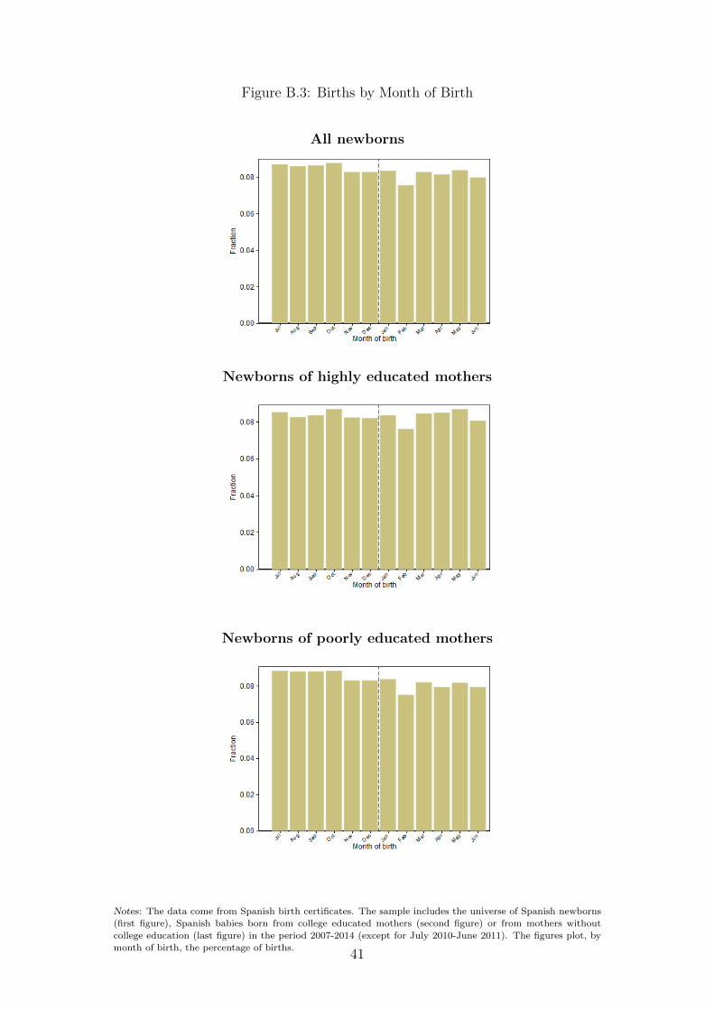
Figure B.3: Births by Month of Birth

All newborns

Newborns of highly educated mothers

Newborns of poorly educated mothers

Notes: The data come from Spanish birth certificates. The sample includes the universe of Spanish newborns

(first figure), Spanish babies born from college educated mothers (second figure) or from mothers without

college education (last figure) in the period 2007-2014 (except for July 2010-June 2011). The figures plot, by

month of birth, the percentage of births.41

Figure B.4: Parental Time Investments by SES and Age: Teaching

05

1015

Low

ess

teac

hing

(m

inut

es p

er d

ay)

0 1 2 3 4 5 6 7 8 9 10 11 12 13 14 15 16 17Age

Non-college educated mothersCollege educated mothers

Notes: Data from the the Spanish Time Use Survey 2003 and 2009. The sample consists of children aged 0 to

17 born in Spain. The figure plots, by age of the children and socioeconomic status, the minutes parents spent

daily with their children doing activities related to teaching.

42

Table B.1: Parental Education/Socioeconomic Status

(1) (2) (3) (4)College mother College mother College mother Index of SES

Birth Certificates STUS EGD PISAYoung (December - January) 0.00962*** -0.0211 0.0147 -0.0104(SE) (0.00191) (0.0205) (0.0152) (0.0183)

Observations 378,624 2,196 3,583 12,311

Notes: Column 1 uses data from the Spanish Time Use Survey 2003 and 2009. The sample is of children aged 0 to 17born in December or January in Spain. Column 2 uses data from the the General Diagnostic Assessment survey 2009.The sample includes Spanish students enrolled in 4th grade. Column 3 uses data from Spanish students aged 15 as-sessed in PISA 2003, 2006, 2009 and 2012. “Young” is an indicator variable that equals one if the student was born inDecember and zero if she was born in January. All the reported models include a vector of dummies for birth cohort.Robust standard errors are in parentheses. *** p<0.01, ** p<0.05, * p<0.1

Table B.2: Birth Characteristics: Children born in January vs December by SES

Children of non-college mothers Children of college educated mothers

December December vs. January December December vs. January

Mean Difference of means SE Mean Difference of means SE

Low-weight (<2500 grams) 0.0898 -0.001 (0.001) 0.0776 0.001 (0.001)Premature 0.0823 0.000 (0.001) 0.0734 0.004** (0.001)C-section 0.24 0.000 (0.002) 0.252 0.003 (0.002)

Observations 239,348 139,276

Notes: Data from Spanish birth certificates, period 2007-2014 (except December 2010 and January 2011). The sample

includes Spanish individuals born in December and January. First 3 columns show the results for the sample of babies

of mothers without college education and the last 3 columns for the sample of babies born from mothers with a college

education. Standard errors are in parentheses. *** p<0.01, ** p<0.05, * p<0.1.

43

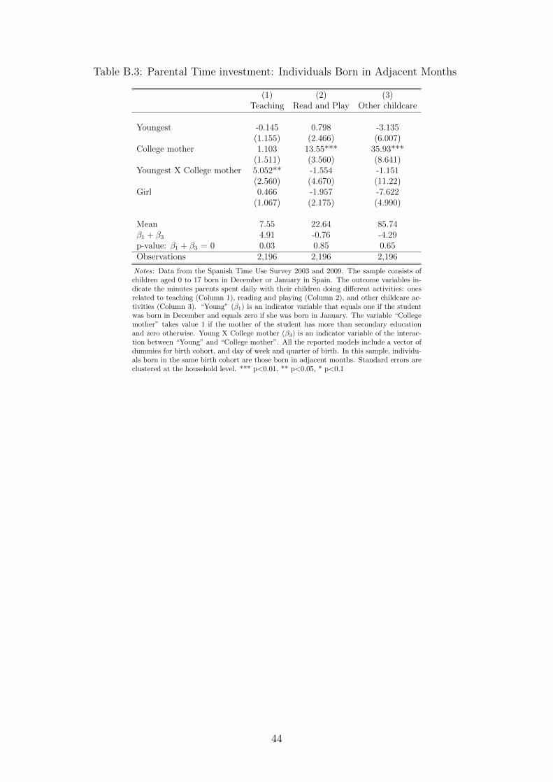
Table B.3: Parental Time investment: Individuals Born in Adjacent Months

(1) (2) (3)Teaching Read and Play Other childcare

Youngest -0.145 0.798 -3.135(1.155) (2.466) (6.007)

College mother 1.103 13.55*** 35.93***(1.511) (3.560) (8.641)

Youngest X College mother 5.052** -1.554 -1.151(2.560) (4.670) (11.22)

Girl 0.466 -1.957 -7.622(1.067) (2.175) (4.990)

Mean 7.55 22.64 85.74β1 + β3 4.91 -0.76 -4.29p-value: β1 + β3 = 0 0.03 0.85 0.65Observations 2,196 2,196 2,196

Notes: Data from the Spanish Time Use Survey 2003 and 2009. The sample consists ofchildren aged 0 to 17 born in December or January in Spain. The outcome variables in-dicate the minutes parents spent daily with their children doing different activities: onesrelated to teaching (Column 1), reading and playing (Column 2), and other childcare ac-tivities (Column 3). “Young” (β1) is an indicator variable that equals one if the studentwas born in December and equals zero if she was born in January. The variable “Collegemother” takes value 1 if the mother of the student has more than secondary educationand zero otherwise. Young X College mother (β3) is an indicator variable of the interac-tion between “Young” and “College mother”. All the reported models include a vector ofdummies for birth cohort, and day of week and quarter of birth. In this sample, individu-als born in the same birth cohort are those born in adjacent months. Standard errors areclustered at the household level. *** p<0.01, ** p<0.05, * p<0.1

44

Table B.4: Parental Time Investment - Summer Excluded

(1) (2) (3)Teaching Reading and Playing Other childcare

Young -0.0309 -0.848 -4.835(1.421) (2.782) (5.816)

College mother 0.839 5.298 16.00**(1.780) (3.714) (8.131)

Young X College mother 7.083** 2.829 -6.154(3.160) (5.003) (10.49)

Girl 0.572 -0.668 -6.687(1.302) (2.311) (4.665)

Mean 9.00 22.43 86.91β1 + β3 7.05 1.98 -10.99p-value: β1 + β3 = 0 0.01 0.63 0.21Observations 1,688 1,688 1,688

Notes: Data from the Spanish Time Use Survey 2003 and 2009 (summer excluded). The sam-ple is of children aged 0 to 17 born in December or January in Spain. The outcome variablesindicate the minutes a day parents spent with their children doing different activities: ones re-lated to teaching (Column 1), reading and playing (Column 2), and other childcare activities(Column 3). “Young” (β1) is an indicator variable that equals one if the student was born inDecember and zero if she was born in January. The variable “College mother” takes value 1if the mother of the student has more than secondary education and zero otherwise. Young XCollege mother (β3) is an indicator variable of the interaction between “Young” and “Collegemother”. All the reported models include a vector of dummies for birth cohort, and day ofweek and quarter of birth. Standard errors are clustered at the household level. *** p<0.01,** p<0.05, * p<0.1

45

Table B.5: Parental Time Investment by Age Groups - Summer excluded

(1) (2) (3) (4) (5) (6) (7) (8) (9)Teaching Reading and Playing Other childcare Teaching Reading and Playing Other childcare Teaching Reading and Playing Other childcare

0-5 6-12 13-17Young 0.232 -5.544 -19.06 -1.125 -1.122 7.636 -0.503 4.470** -2.960

(2.042) (8.344) (16.47) (2.909) (3.749) (7.512) (2.041) (2.100) (5.071)College mother 3.018 6.859 27.75* -2.491 7.821* 18.24* 2.153 1.439 -4.154

(2.677) (8.245) (16.28) (3.473) (4.375) (10.77) (2.587) (1.685) (4.904)Young X Collegemother -2.330 7.990 -8.467 15.93*** 2.166 -10.01 6.360 -4.741 11.33

(3.724) (11.40) (23.68) (6.001) (6.440) (14.01) (6.142) (3.488) (7.127)Girl 0.727 -0.663 -8.534 0.130 -0.243 -12.56** 1.229 -2.322 -4.097

(1.769) (5.780) (10.54) (2.362) (2.986) (6.222) (1.952) (1.607) (4.332)

Mean 5.50 45.31 171.88 14.73 15.93 65.01 5.54 3.98 15.33β1 + β3 -2.10 2.45 -27.53 14.81 1.04 -2.37 5.86 -0.27 8.37p-value: β1 + β3 = 0 0.49 0.77 0.14 0.01 0.83 0.84 0.30 0.91 0.14Observations 569 569 569 639 639 639 480 480 480

Notes: Data from the Spanish Time Use Survey 2003 and 2009 (summer excluded). The sample is of children aged 0 to 17 born in December or January in Spain. The first 3 columns include only children youngerthan 6, columns 4 to 6 include children aged 6 to 12 and the last 3 columns include children aged 13 to 17. The outcome variables indicate the minutes a day parents spent with their children doing different activities:ones related to teaching, to reading and playing, and other childcare activities. “Young” (β1) is an indicator variable that equals one if the student was born in December and equals zero if she was born in January. Thevariable “College mother” takes value 1 if the mother of the student has more than secondary education and zero otherwise. Young X College mother (β3) is an indicator variable of the interaction between “Young”and “College mother”. All the reported models include a vector of dummies for birth cohort, and day of week and quarter of birth. Standard errors are clustered at the household level. *** p<0.01, ** p<0.05, * p<0.1

46

Table B.6: School Choice

(1) (2)Parental survey Student survey

Young 0.0194 0.00643(0.0220) (0.0193)

College mother -0.0907*** -0.0189(0.0298) (0.0224)

Young X College mother -0.0455 -0.0640**(0.0386) (0.0315)

Girl 0.00401 -0.0205(0.0177) (0.0152)

Mean 0.47 0.24β1 + β3 -0.026 -0.058p-value: β1 + β3 = 0 0.41 0.02

Observations 3292 3292

Notes: The data come from the General Diagnostic Assessment survey2009. The sample includes Spanish students enrolled in 4th grade whowere born in December or January. The outcome variables is an indicatorof whether the parent (Column 1) or the student (Column 2) declare (inseparate surveys) if the student is enrolled in her current school becauses/he lives in the school’s catchment area. “Young” (β1) is an indicatorvariable that equals one if the student was born in December and zeroif she was born in January. The variable “College mother” takes value 1if the mother of the student has a college education and zero otherwise.Young X College mother (β3) is an indicator variable of the interactionbetween “Young” and “College mother”. Standard errors are clustered atthe school level. * p<0.10, ** p<0.05, *** p<0.01

47

Table B.7: School Quality Index

School quality index Private school Class size Peers motivated to learn Teacher quality index Family peers motivation index

(1) (2) (3) (4) (5) (6) (7) (8) (9) (10)Teachers Teachers target Teachers follow Parents attend Parental interest Parental interest

continual training students with students’ progress daily meetings in learning problems in gradeslearning disadvantages

Young -0.0154 0.00610 -0.0495 -0.0540 -0.0559 -0.0167 0.0547 -0.000693 -0.0111 -0.0119(0.0180) (0.0437) (0.0415) (0.0450) (0.0441) (0.0434) (0.0441) (0.0425) (0.0444) (0.0437)

College mother 0.00331 0.0272 0.00164 0.00686 0.0128 -0.0245 0.0225 -0.0192 -0.00843 0.0109(0.0238) (0.0608) (0.0728) (0.0628) (0.0560) (0.0630) (0.0607) (0.0634) (0.0648) (0.0655)

Young X College mother 0.106 *** 0.0719 0.143 * 0.155 ** 0.166 ** 0.158 ** -0.0287 0.154 ** 0.0181 0.116(0.0299) (0.0755) (0.0843) (0.0775) (0.0727) (0.0804) (0.0760) (0.0747) (0.0779) (0.0786)

Girl 0.00382 0.0338 -0.0354 -0.0175 0.00120 0.00485 0.0186 0.00287 -0.000826 0.0267(0.0133) (0.0357) (0.0336) (0.0351) (0.0342) (0.0350) (0.0355) (0.0352) (0.0343) (0.0343)

Mean 0.01 0.03 -0.01 -0.02 0.00 0.00 0.02 0.02 0.01 0.02β1 + β3 0.09 0.08 0.09 0.10 0.11 0.14 0.03 0.15 0.01 0.10p-value: β1 + β3 = 0 0.00 0.23 0.19 0.13 0.10 0.03 0.68 0.02 0.92 0.12

Observations 3171 3171 3171 3171 3171 3171 3171 3171 3171 3171

Notes: The data come from the General Diagnostic Assessment survey 2009. The sample includes Spanish students enrolled in 4th grade who were born in December or January. The outcome variables are an Index of School Quality (Column 1) and the different schoolcharacteristics that are included in such index: a concertada school indicator (Column 2), class size (Column 3), an indicator of whether the teacher reports that the students in her class are very motivated (Column 4), variables related to teacher quality (columns 5 to 7) andto parental involvement (columns 8 to 10). “Young” (β1) is an indicator variable that equals one if the student was born in December and zero if she was born in January. The variable “College mother” takes value 1 if the mother of the student has a college education andzero otherwise. Young X College mother (β3) is an indicator variable of the interaction between “Young” and “College mother”. Standard errors are clustered at the school level. * p<0.10, ** p<0.05, *** p<0.01

48

Table B.8: Parental Time Investment by Student Gender

Boys Girls

(1) (2) (3) (4) (5) (6)Teaching Read and Play Other childcare Teaching Read and Play Other childcare

Youngest -1.093 -1.018 -4.428 -1.720 1.133 7.759(2.222) (3.161) (6.745) (1.972) (2.593) (5.541)

College mother -3.809 4.462 -2.342 3.280 2.328 8.331(2.554) (3.944) (7.729) (2.855) (3.108) (8.409)

Youngest X College mother 14.37*** 4.280 10.96 4.423 0.276 -10.28(5.153) (5.834) (11.35) (4.733) (5.085) (11.96)

Mean 8.91 11.65 44.5 9.03 10.15 39.4β1 + β3 13.277 3.262 6.532 2.703 1.409 -2.521p-value: β1 + β3 = 0 0.0066 0.4977 0.4767 0.5247 0.731 0.8036Observations 723 723 723 729 729 729

Notes: Data from the Spanish Time Use Survey 2003 and 2009. The sample is of children aged 6 to 17 born in December or January in Spain.The first 3 columns correspond to the analysis of the sample of boys and the last 3 to the sample of girls. The outcome variables indicate theminutes a day parents spent with their children doing different activities: ones related to teaching, to reading and playing, and other childcareactivities. “Young” (β1) is an indicator variable that equals one if the student was born in December and zero if she was born in January. Thevariable “College mother” takes value 1 if the mother of the student has more than secondary education and zero otherwise. All the reportedmodels include a vector of dummies for birth cohort, and day of week and quarter of birth. Young X College mother (β3) is an indicator variableof the interaction between “Young” and “College mother”. Standard errors are clustered at the household level. *** p<0.01, ** p<0.05, * p<0.1

49