Polytechnic University, Brooklyn, NY ©2002 by H.L. Bertoni1 X. Numerical Integration for Propagation Past Rows of Buildings Adapting the physical optics

Polytechnic University, Brooklyn, NY

©2002 by H.L. Bertoni 1

X. Numerical Integration for Propagation Past Rows of Buildings

• Adapting the physical optics integrals for numerical evaluation

• Applications– Computed height dependence of the fields

– Buildings with flat roofs

– Buildings of random height, spacing– Rows of building on hills

– Trees located next to buildings

– Penetration through buildings at low frequencies



Numerical Integration for Field Variation in 2D

H(xn+1,yn+1) =ejπ / 4

λH(xn,yn)

jke−jkρn

ρndyn

hn

∞

∫ , ρn = (xn+1 −xn)2 +(yn+1 −yn)

2

• How to terminate the numerical integration without changing the computed field– Abrupt termination like an absorbing screen above the termination point.

– Make the field go smoothly to zero above the significant region

• Discretize the integral in step size of at least /2

n

n

yn

x

n=1 n=2 n=3 n n+1

€

E

€

H

Incidentwave

yn+1

dn



Termination Strategy• Multiply Hn(yn) by the neutralizer function (yn) to smoothly reduce the integration to

zero in order to avoid the spurious contribution given by abrupt termination of the integral.

€

η yn( )=

1 for yn <yc

exp− yn −yc( )2/w2

[ ] ; yc <yn <yc +3w

0 for yn >yc +3w

⎧

⎨ ⎪

⎩ ⎪

yc >Ndtanα + Ndλ secα3w

exp−yn −yc( )2/w2

[ ]

Hn yn( ) η yn( )



Discretization

€

Hn+1 yn+1( )=e jπ /4

λη yn( )Hn yn( )

e−jkρn

ρndyn

0

ym

∫

where

ρn = xn+1 −xn( )2+ yn+1 −yn( )

2

Define

φ yn( ) =∠Hn yn( )−kρn and A yn( )=η yn( )Hn yn( )1λρn

Then

Hn+1 yn+1( )=e jπ /4 A yn( )ejφ yn( )dyn

mΔ

(m+1)Δ

∫m=0

M

∑Using the linear approximations

φ yn( ) ≈φ mΔ( )+ φ mΔ+Δ( )−φ mΔ( )[ ]yn −mΔ

Δ

A yn( ) ≈A mΔ( )+ A mΔ+Δ( )−A mΔ( )[ ]yn −mΔ

Δ



Discretization - cont.

€

The integration in each interval can be evaluated in closed form so that

Hn+1 pΔ( ) =Δe jπ /4 A mΔ+Δ( )e jφ mΔ +Δ( ) −A mΔ( )eφ mΔ( )

φ mΔ+Δ( )−φ mΔ( )

⎧ ⎨ ⎩ m=0

M

∑

+jA mΔ+Δ( )−A mΔ( )

φ mΔ+Δ( )−φ mΔ( )[ ]2 e jφ mΔ+Δ( ) −eφ mΔ( )[ ]

⎫ ⎬ ⎭



Height Variation of the Field Above the M=120 Row of Buildings for Plane Wave Incidence

(= 1o, d = 50 m, f = 900 MHz, M = 120 > N0 )

Dashed curve for y < 0 is ( ) θTp DgQ )(2

0.0

0.2

0.4

0.6

0.8

1.0

1.2

1.4

1.6

1.8|H

(y)|

-30 -20 -10 0 10 20 30 40 50 60

Height in wavelength y/

K.H.UTD

Q(gp)



Standing Wave Behavior for y > 0 (= 1o, d = 50 m, f = 900 MHz, M = 120 > N0 )

|H(y

)|

Height in wavelength y/

0.00.20.40.60.81.01.21.41.61.8

-30-20-10 0 10 20 30 40 50 60

y

€

Height variation e jκy +Γe−jκy =1+Γe−j2κy where κ =ksinα

Separation Δy between minima is 2κΔy=2π or

Δy=π κ =π ksinα =λ 2sinα

For α =1o, Δy=28.6λ

Also, 1+Γ ≈1.6 and 1- Γ ≈0.4 so that Γ ≈0.6



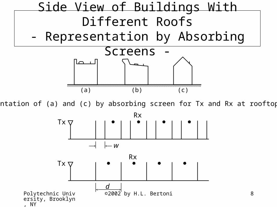
Side View of Buildings With Different Roofs- Representation by Absorbing Screens -

Representation of (a) and (c) by absorbing screen for Tx and Rx at rooftop height

(a) (b) (c)

w

TxRx

RxTx

d



Effect of Roof Shape on Reduction Factor QComputed Midway Between Rows

Constant offset of 3.3 dBbetween two case (a) and (c),but no change in range index n.



Shadow Fading

• Variation from building-to-building along along a row

• Variation from row-to-row

• Why the shadow fading is lognormal ?



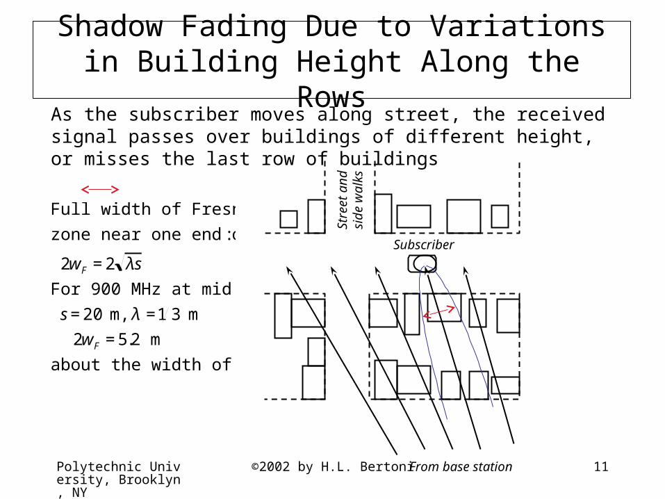
Shadow Fading Due to Variations in Building Height Along the Rows

As the subscriber moves along street, the received signal passes over buildings of different height, or misses the last row of buildings

Stre

et a

ndsi

de w

alks

Subscriber

From base station

€

Full width of Fresnel

zone near one end of link:

2wF =2 λs

For 900 MHz at mid street

s=20 m, λ =1 3 m

2wF =5.2 m

about the width of a house



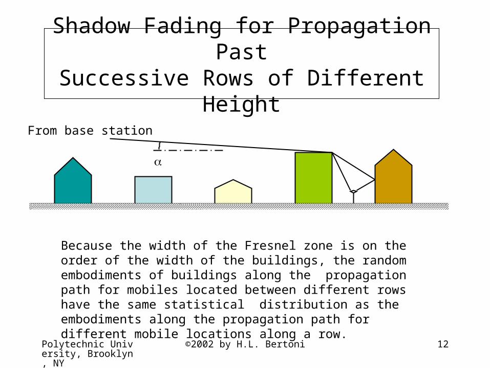
Shadow Fading for Propagation PastSuccessive Rows of Different Height

From base station

Because the width of the Fresnel zone is on the order of the width of the buildings, the random embodiments of buildings along the propagation path for mobiles located between different rows have the same statistical distribution as the embodiments along the propagation path for different mobile locations along a row.



Modeling Shadow Fading for Random Building Height

IncidentPlane wave

x

y

• Building height determined by random number generator

• Use numerical integration to find fields at successive screen, mobiles



Row-to-Row Variation of Rooftops FieldDue to Random Building Height

Plane wave incidence ( f = 900 MHz, = 0.5º, d = 50 m )HB uniformly distributed 8 - 14 m

1.0

0.9

0.8

0.7

0.6

0.5

0.4

0.3

0.2

0.1

0.0100 110 120 130 140 150

Screen number

H( y

)



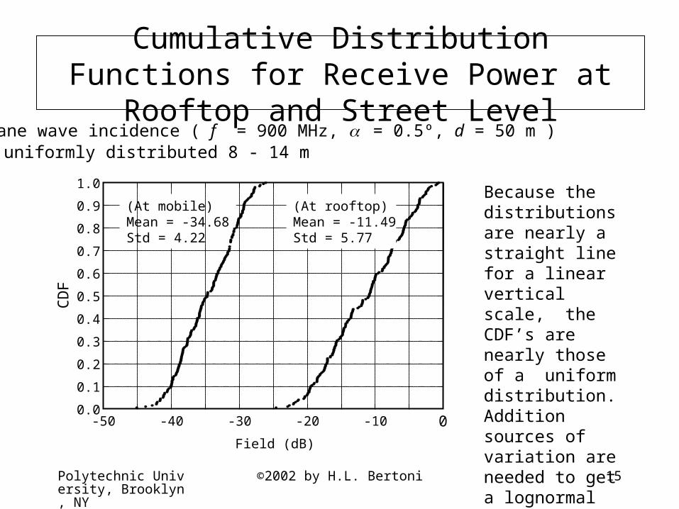
Cumulative Distribution Functions for Receive Power at Rooftop and Street Level

Plane wave incidence ( f = 900 MHz, = 0.5º, d = 50 m )HB uniformly distributed 8 - 14 m

1.0

0.9

0.8

0.7

0.6

0.5

0.4

0.3

0.2

0.1

0.0-50 -40 -30 -20 -10 0

Field (dB)

CD

F

(At mobile)Mean = -34.68Std = 4.22

(At rooftop)Mean = -11.49Std = 5.77

Because the distributions are nearly a straight line for a linear vertical scale, the CDF’s are nearly those of a uniform distribution. Addition sources of variation are needed to get a lognormal distribution.



Missing Buildings, Roof Shape and BuildingMaterials Also Cause Signal Variation

Additional sources of variability that influence diffraction down to the mobile are roof characteristics and construction, and the absence of buildings in a row, such as at and intersection. For simulations we assume: 50% peaked, 50% flat 50% conducting, 50% absorbing boundary conditions 10% of buildings are missing

hBS hm

HB

d



Cumulative Distribution Function for Combinationof Random Height and Other Random Factor

CDF of the received power at Street levelfor:

f = 900 MHz = 0.5°d = 40 mHB distribution is Uniform Rayleigh Nearly straight line for the distorted vertical scale indicates a Normal distribution of power in dB.



Dependence of Standard Deviation of Signal Distribution on HB for 900 MHz and 1.8 GHz



Why Shadow Fading is Lognormal Distributed

• Sequence of random processes, each of which multiply the signal by a random number: - Random building height - Random diffraction down to mobile due to roof shape, construction, missing buildings

• On dB scale, multiplication of random numbers is equal to addition of their logs

• By central limit theorem of random statistics, a sum of random numbers has normal (Gaussian) distribution

• Adding just two random numbers gives normal distribution, except in tails

Documents

Polytechnic University, Brooklyn, NY ©2002 by H.L. Bertoni1 X. Numerical Integration for Propagation Past Rows of Buildings Adapting the physical optics