Polypyridyl Transition Metal Complexes with Application in

Water Oxidation Catalysis and Dye-Sensitised Solar Cells

Inauguraldissertation

zur

Erlangung der Würde eines Doktors der Philosophie

vorgelegt der

Philisophisch-Naturwissenschaftlichen Fakultät

der Universität Basel

von

Jennifer A. Rudd

aus England

Basel 2012

Genehmigt von der Philosophisch‐Naturwissenschaftlichen Fakultät der Universität

Basel auf Antrag der Herren Professoren und Herr Doktor

Prof. Dr. E. C. Constable Dr. N. Robertson

Basel, den 13.11.2012

Prof. Dr. J. Schibler

Dekan

Original document stored on the publication server of the University of Basel edoc.unibas.ch

This work is licenced under the agreement „Attribution Non-Commercial No Derivatives – 2.5 Switzerland“. The complete text may be viewed here:

creativecommons.org/licenses/by-nc-nd/2.5/ch/deed.en

ABCCDBEFADEDDFE

EDDD

ABCDEFFEF

D!DFF"B

FFBAFFECFAFCCCECC

ABCCDBEFCFAAFBB

ADEDCDDFEBF

CEFFFDCAFAFCEFFFFFB

C!AEFFAF!EFCBFFABCFE

"FFFFAFBFFA#F

$%B%&&AF!A&FA&C'A'E&()&A&EE *%+,(--.

EDEF"E!D"!EDE#EDBD#!DED

FF'EC/0EFA!FF1%B%&&AF!A&FA&C'A'E&()&A&AEE

BFECD0*EFFA2FFBCECAEEF/0EFAFF'E3BFFCFF'FECFA/0EF*EF!DEFAEBBFAFA0F!0FFEEB!FE!FA*FFFDEFBCFDFFF0*EEAC'AFFFB

„Und Gott sprach: Es werde Licht! und es ward Licht.

Und Gott sah, daß das Licht gut war.

Da schied Gott das Licht von der Finsternis“

1 Mose 1 vs 3-4, Luther Bibel 1545

“God spoke “Light!” and light appeared.

God saw that light was good and separated light from dark.”

Genesis 1 vs 3-4, The Message translation

i

Acknowledgements

First and foremost thank you to Prof. Ed. Constable for giving me a place in the research

group, for freedom to explore the world of chemistry and for all his help, support and

kindness over the last three years.

I can no longer count the number of hours of discussion Prof. Catherine Housecroft and I

have had sat in her office. Thank you for all of them and all of your proof-reading of this

manuscript.

Thank you to Dr Robertson for agreeing to be my examiner and travelling from

Edinburgh to do so.

Thank you to Prof. Markus Meuwly for giving me a place in his research group for a few

months to run my own calculations and for the countless subsequent discussions on basis

sets, calculating absorption spectra and how to please referees when publishing.

Dr. Jennifer Zampese and Dr. Markus Neuburger have measured all my crystals and have

done their best to help me understand where the results come from and what they mean.

Dr. Michael Devereux was kind enough to run the DFT calculations on my ruthenium

complexes and was very patient in teaching me how to read output files, use GaussSum

and Molekel.

Dr Emma Dunphy got me started on the ruthenium project and has always been a

massive encouragement and a great photophysics teacher. Thanks for all of our Skype,

lab and gmail conversations about all things chemistry.

Thank you to Dr. Biljana Bozic-Weber, Liselotte Siegfried and Ewald Schönhofer for all

of their work making and measuring the solar cells.

Thanks must also go to Prof. Craig Hill, Dr. Yurii Geletii and Hongjin Lv of Emory

University (Atlanta) for the water oxidation collaboration.

ii

Dr. Niamh Murray, Dr. Colin Martin and Dr. Iain Wright have been great post-docs and

have also spent their time checking and suggesting improvements for this manuscript.

Thank you. Iain is thanked particularly for help with the spectroelectrochemistry.

The old members of lab 217 made the Constable group a very amusing and interesting

place to be in my first couple of years here.

Dr Kate Harris, I still miss you sitting on the opposite side of the lab to me.

Thank you to Constable group members past and present, particularly for ESI/MALDI

and VT-NMR measurements, to the Meuwly group and to all of the chemistry department

support team.

Beatrice without you I wouldn’t have my Ausländerausweis in the first place (do you

remember shouting at the people in the Spiegelhof down the phone?) and your help with

the ever present Swiss paperwork has been invaluable throughout the last three years.

Thanks to the Swiss National Science Foundation and the European Research Council

(Advanced Grant 267816 LiLo) for financial support.

A massive thank you to the Rock Solid youth and team past and present. My Basel

experience would not have been the same without you and I have been blessed

throughout my time with all of you. Zech. 4 vs 6 “Not by might, nor by power, but by my

Spirit, says the Lord Almighty”

My parents have supported me throughout and it’s great knowing you’re always there.

Thomas thanks for always making me feel better about my research and Clare, thank you

for all your crazy texts, post and encouragement along the way.

Last but certainly not least - Jason, thank you for saying “yes dear” to all of my PhD

neuroses and all of your support through every stage. With you by my side everything is

better.

iii

Abstract

This thesis contains complementary synthetic and computational studies of transition

metal complexes with polypyridyl ligands for use either as water oxidation catalysts or

for application in dye-sensitised solar cells (DSSCs).

Chapter 1 introduces the reasons for researching water splitting catalysts and describes a

number of current techniques used to do so; from photoelectrochemical cells to the use of

transition metal polypyridyl complexes. It also introduces three commercially available

types of solar cells; silicon, thin film and the dye-sensitised solar cell.

Chapter 2 describes the synthesis of seven ruthenium(II) complexes with substituted

4'-(4-pyridyl)-2,2':6',2''-terpyridine ligands and their photophysical and electrochemical

properties. Density Functional Theory (DFT) calculations were used to explore the

compositions of the highest occupied- and lowest unoccupied molecular orbitals (HOMO

and LUMO, respectively) and Time Dependent DFT (TD-DFT) was used to predict the

absorption spectra of the complexes.

Chapter 3 contains information on water soluble ruthenium(II) complexes, their

synthesis, photophysical and electrochemical properties and their activity as water

splitting co-catalysts. A mechanism to explain the variable activities of the complexes is

also put forward.

Chapter 4 describes the synthesis of two homoleptic Cu(I) complexes. One complex

involves a simple 6,6'-dimethyl-2,2'-bipyridine ligand. The other complex contains a

ligand with extended π-conjugation. The properties of the Cu(I) complexes are studied in

terms of their suitability for use in DSSCs. A strategy of ligand-exchange on the surface

of titanium dioxide (TiO2) is then utilised to form surface-bound heteroleptic Cu(I)

complexes and efficiences of these complexes in DSSCs were measured.

iv

Chapter 5 details the development of a suitable basis set to be used in both DFT and TD-

DFT to predict the absorption spectra of the homoleptic Cu(I) complexes in Chapter 4

and the accuracies of the predicted spectra are assessed. The properties of the

uncharacterised, heteroleptic Cu(I) complexes were then predicted and the effects of the

anchoring ligands on the overall properties of the complexes were assessed.

Chapter 6 describes the synthesis of two mono-substituted bipyridine-based ligands and

their corresponding homoleptic chiral copper(I) complexes. Variable temperature nuclear

magnetic resonance (VT-NMR) experiments are described, along with the photophysical

properties of the ligands and complexes.

Chapter 7 consists of the overall conclusions and an outlook.

Parts of this work have been published in:

“Water-soluble alkylated bis4′-(4-pyridyl)-2,2′:6′,2′′-terpyridineruthenium(II)

complexes for use as photosensitizers in water oxidation: a complementary experimental

and TD-DFT investigation”

Edwin C. Constable, Michael Devereux, Emma L. Dunphy, Catherine E. Housecroft,

Jennifer A. Rudd and Jennifer A. Zampese, Dalton Trans., 2011, 40, 5505-5515

“Exploring copper(I)-based dye-sensitized solar cells: a complementary experimental and

TD-DFT investigation”

Biljana Bozic-Weber, Valerie Chaurin, Edwin C. Constable, Catherine E. Housecroft,

Markus Meuwly, Markus Neuburger, Jennifer A. Rudd, Ewald Schönhofer and

Liselotte Siegfried, Dalton Trans., 2012, 41, 14157-14169

v

Abbreviations

Å Angstrom

bpy 2,2'-bipyridine nBu n-Butyl tBu t-Butyl

calc. calculated

COSY correlation spectroscopy

CPCM conductor-like polarisable continuum model

CV cyclic voltammetry

δ chemical shift

D deuterium

DFT density functional theory

dmbpy 6,6'-dimethyl-2,2'-bipyridine

DSSC dye-sensitised solar cell

E standard half-cell potential

ε absorption coefficient in mol dm-3 cm-1

EA elemental analysis

Eh Hartree

eq. equivalent

ESI electrospray ionization

Et ethyl

eV electron volt

ff fill factor

η overall conversion efficiency from solar to electrical energy for a

photovoltaic device

HF Hartree-Fock

HMBC heteronuclear multiple bond configuration

HMQC heteronuclear multiple quantum coherence

HOMO highest occupied molecular orbital

Hz hertz

ic internal conversion

ILCT intra-ligand charge transfer

vi

Isc short circuit current

isc intersystem crossing

IR infra-red (s, strong; m, medium; w, weak)

ITO indium tin oxide

J coupling constant

K Kelvin

λem emission wavelength

λex excitation wavelength

λmax wavelength at maximum absorbance

L ligand

LC ligand centered transition

LLCT ligand to ligand charge transfer

LMCT ligand to metal charge transfer

LUMO lowest unoccupied molecular orbital

M parent ion

MALDI-TOF matrix assisted laser desorption ionisation – time of flight

MC metal centred transition

MLCT metal to ligand charge transfer

mmol milimol

MO molecular orbital

MS mass spectrometry

mV millivolt

m/z mass to charge ratio

N3 [Ru(4,4'-(dicarboxy)-2,2'-bipyridine)2(SCN)2]

N719 [Ru(4,4'-(dicarboxy)-2,2'-bipyridine)2(SCN)2][TBA]2

nHOMO next highest occupied molecular orbital

NIST National Institute of Standards and Technology

nm nanometre

NMR nuclear magnetic resonance (signals identified as d, dd, t, m, br which

mean doublet, doublet of doublets, triplet, multiplet and broad,

respectively)

NOESY nuclear Overhauser enhancement spectroscopy

PCM polarisable continuum model

vii

Ph phenyl

ppm parts per million

qpy 2,2':6',2″:6″,2‴-quaterpyridine

rt room temperature

SCN thiocyanate

TBA tetrabutylammonium

TBAPF6 tetrabutylammonium hexafluoridophosphate tBu tert-butyl

TD-DFT time dependent density functional theory

TFL Transport for London

THF tetrahydrofuran

TiO2 titanium dioxide

TLC thin layer chromatography

TMS trimethylsilane

tpy 2,2';6',6''-terpridine

UV ultraviolet

V volt

vis visible

Voc open circuit voltage

vs. Versus

VT-NMR variable temperature NMR

WOC water oxidation catalyst

viii

General Experimental Section

1H and 13C NMR spectra were recorded on a Bruker DRX-500 MHz NMR spectrometer;

chemical shifts are referenced to residual solvent peaks with TMS = δ 0 ppm.

MALDI-TOF mass spectra were recorded on a PerSeptive Biosystems Voyager

spectrometer. Electrospray mass spectra were recorded on a Bruker esquire 3000plus.

Electronic absorption and emission spectra were recorded using an Agilent 8453

spectrophotometer and Shimadzu RF-5301 PC spectrofluorometer, respectively. Solution

lifetime measurements were made using an Edinburgh Instruments mini-τ apparatus

equipped with an Edinburgh Instruments EPLED-300 pico-second pulsed diode laser

(λex = 467 or 404 nm, pulse width = 75.5 or 48.2 ps, respectively) with the appropriate

wavelength filter. The quantum yields were measured with an absolute PL quantum yield

spectrometer C11347 Quantaurus_QY from Hamamatsu.

Solid state electronic absorption spectra of Cu(I)-containing dyes on TiO2 were measured

using a Varian Cary 5000 with a conducting glass with a TiO2 layer as a blank.

TGA-MS measurements were carried out on a Mettler Toledo TGA/SDTA851e with

Pfeiffer Vacuum ThermostarTM.

IR spectra were recorded on a Shimadzu FTIR-8400S spectrophotometer (solid samples

on a Golden Gate diamond ATR accessory).

In chapter 2 electrochemical measurements were carried out using an Eco Chemie

Autolab PGSTAT system with glassy carbon working and platinum auxiliary electrodes;

a silver wire was used as a pseudo-reference electrode. Solvent was dry, purified MeCN

and 0.1M [nBu4N][PF6] was used as supporting electrolyte. An internal reference of

Cp2Fe was added at the end of each experiment.

In chapter 3 electrochemical measurements were carried out using an Eco Chemie

Autolab PGSTAT system with a Ag/AgCl working electrode and a Pt counter electrode .

Solvent was deionised water and NaHSO4 was used as the supporting electrolyte.

ix

In chapter 4 electrochemical data were recorded using a CH Instruments potentiostat

(model 900B) with glassy carbon working and platinum auxiliary electrodes; a silver

wire was used as a pseudo-reference electrode. Solvents for the electrochemistry were

dry and purified, and the supporting electrolyte was 0.1 M [nBu4N][PF6]; an external

reference of Cp2Fe was measured at the start and again at the end of each experiment.

x

Table of Contents Chapter 1 Introduction 1.1 General Introduction 1

1.2 Water Splitting 1

1.3 Solar Cells 6

1.4 References 10

Chapter 2 Alkylated bis 4’-(4-pyridyl)-2,2':6',2''-terpyridineruthenium(II)

complexes

2.1 Introduction 12

2.2 Synthesis of [Ru(R-pytpy)2][PF6]4 Complexes 16

2.3 Results and Discussion 18

2.3.1 1H NMR Spectroscopy 18

2.3.2 13C1H NMR Spectroscopy 21

2.3.3 Mass Spectrometry 23

2.3.4 Absorption Spectroscopy 23

2.3.5 Emission Spectroscopy 25

2.3.6 Electrochemistry 27

2.3.7 Crystal Structures 30

2.4 DFT and TD-DFT Calculations 40

2.5 Conclusion 46

2.6 Experimental 47

2.7 References 53

Chapter 3 Water soluble alkylated bis4'-(4-pyridyl)-2,2':6',2" -

terpyridineruthenium(II) complexes for application as water oxidation

catalysts.

3.1 Introduction 55

3.2 Synthesis of [Ru(R-pytpy)2][HSO4]4 Complexes 61

xi

3.3 Results and Discussion 62

3.3.1 1H NMR Spectroscopy 62

3.3.2 13C1H NMR Spectroscopy 64

3.3.3 Mass Spectrometry 65

3.3.4 Elemental Analysis and Thermogravimetric Analysis 65

3.3.5 Absorption Spectroscopy 66

3.3.6 Emission Spectroscopy 68

3.3.7 Electrochemistry 70

3.3.8 Water Oxidation Activity 72

3.4 Conclusion 75

3.5 Experimental 76

3.6 References 81

Chapter 4 Copper(I) Polypyridyl Complexes for Application in DSSCs.

4.1 Introduction 83

4.2 Synthesis of ligand 9 and corresponding Cu(I) complexes 91

4.3 Results and Discussion 93

4.3.1 1H NMR Spectroscopy 93

4.3.2 13C1H NMR Spectroscopy 100

4.3.3 Mass Spectrometry 103

4.3.4 Absorption Spectroscopy 104

4.3.5 Excitation and Emission Spectroscopy 106

4.3.6 Electrochemistry 110

4.3.7 Crystal Structures 114

4.3.8 DSSCs Incorporating the Cu(I) Complexes 121

4.4 Conclusions 123

4.5 Experimental 124

4.6 References 128

Chapter 5 A DFT and TD-DFT investigation of Cu(I) polypyridyl complexes with

application in DSSCs

xii

5.1 Introduction 130

5.2 Calculation Details 134

5.3 Results and Discussion 135

5.4 Conclusions 155

5.5 References 156

5.6 Appendix 157

Chapter 6 Cu(I) complexes with pendant pyridyl functionalities for application in

DSSCs

6.1 Introduction 166

6.2 Synthesis – Ligands 168

6.3 Results and Discussion (I) 170

6.3.1 1H NMR Spectroscopy – Ligands 170

6.3.2 13C1H NMR Spectroscopy- Ligands 172

6.3.3 Mass Spectrometry – Ligands 174

6.3.4 Absorption Spectroscopy – Ligands 175

6.3.5 Emission and Excitation Spectroscopy – Ligands 176

6.3.6 Crystal Structures – Ligands 177

6.4 Synthesis - Cu(I) Complexes 182

6.5 Results and Discussion (II) 182

6.5.1 Section Introduction 182

6.5.2 1H NMR Spectroscopy – Cu(I) Complexes 183

6.5.3 Mass Spectrometry – Cu(I) Complexes 189

6.5.4 Absorption Spectroscopy – Cu(I) Complexes 189

6.5.5 Emission and Excitation Spectroscopy – Cu(I) Complexes 191

6.5.6 Crystal Structures – Cu(I) Complexes 191

6.6 Conclusions 194

6.7 Experimental 195

6.8 References 199

Chapter 7 Conclusions and Outlook 200

1

Chapter 1

Introduction

1.1 General Introduction

The world’s fossilised energy resources are finite and the impact of their use is already

being felt worldwide. Global warming, melting ice caps and repeated flash flooding are

all symptoms of human dependence on fossil fuels to provide the 14 terawatts (TW) of

power that are used every year1. In order to reduce such dependence, alternative fuel

sources, such as hydrogen gas for use in fuel cells, are being developed by means of the

catalytic splitting of water – a focus of this thesis. Nuclear power, wind turbines, tidal

barriers, geothermal energy, hydroelectric dams and biogas are also in use, along with the

other focus of this thesis: solar cells.

1.2 Water Splitting

Water splitting (Eqn. 1.1) is a process carried out in plants by means of photosynthesis.

(Eqn. 1.1)

In photosynthesis sunlight is absorbed by a plant and the energy from the sunlight is

converted into chemical energy whereupon carbon dioxide and water are converted into

sugars and molecular oxygen (Eqn. 1.2).

(Eqn 1.2)

This process provides ~130 TW of power per year2, which is far more than is consumed

by the human race. For this reason research has recently blossomed in the area of

artificial photosynthesis – chemically mimicking photosynthesis. This process is a way of

producing hydrogen that can then be stored and used as a source of fuel.

2

Hydrogen is becoming more common as a fuel source for road transport. BMW recently

manufactured 100 test cars (BMW Hydrogen 7) which can be powered by either petrol or

hydrogen3. The cars have conventional internal combustion engines, which can burn

either petrol or hydrogen in the cylinders. Honda have developed a car (Honda FX

Clarity) which runs on electricity, which is produced from the combination of hydrogen

and oxygen (Eqn. 1.3) by means of a fuel cell4. A fuel cell is a device that converts

chemical energy from a fuel to electrical energy by means of a chemical reaction with

oxygen or another oxidising agent5.

(Eqn. 1.3)

The same technology is used in the newest fleet of London buses, which were introduced

in 20116. The fuel cell that combines the hydrogen and oxygen works at

40-60 % efficiency and the only emission from the bus is water vapour.

Hydrogen is also used as a feedstock for the synthesis of fertilisers, pharmaceuticals and

plastics.

As the demand for hydrogen grows, more efficient ways of generating hydrogen are

needed. There are multiple ways of photochemically splitting water (Eqn. 1.1) to generate

molecular hydrogen and molecular oxygen7-14

, for example: photoelectrochemical cells,

heterogeneous catalysis involving semiconductor particles with co-catalysts attached,

quantum dots and homogeneous catalysis using dyes.

The workings of a photoelectrochemical cell are depicted in Fig. 1.1.

3

Fig. 1.1 Schematic of a photoelectrochemical cell redrawn from ref [10

].

Fujishima and Honda were the first to report this method of water splitting15

. Titanium

dioxide (TiO2) in the rutile form was used as the semiconductor electrode in conjunction

with nanoparticulate platinum (Pt) as the counter electrode. On illumination there is hole-

electron separation within the TiO2 nanoparticles. The holes oxidise water to molecular

oxygen and protons. The electrons migrate to the Pt counter electrode where the protons

are reduced to molecular hydrogen. The photoelectrochemical cell only absorbs light in

the UV region of the spectrum as TiO2 has such a large bandgap energy (3 eV).

Since the discovery by Fujishima and Honda, work has been carried out on substituting

the TiO2 in the photoelectrochemical cell for another substrate or substrates which will

absorb visible light. This work has been the subject of recent reviews7, 9

. Methods such as

chemical doping or the use of more than one semiconductor in parallel are being

developed. The advantage of these newer systems is that they absorb visible light and

therefore have a higher efficiency than the Fujishima/Honda system. However, the

chemically doped and parallel systems tend to be much less stable.

O2 Out

H2 Out

Power Source

Electrolyte

Counter-electrode

Window

Semi conductor electrode

hν H+ ion permeable membrane

4

Another approach to splitting water is the use of heterogeneous catalysts. The advantages

of heterogeneous catalysis over the photoelectrochemical cell are that there is no need for

direct illumination or transparent materials, which can often be expensive.

The heterogeneous catalyst can be prepared in one of two ways16

;

(i) Both the water oxidation catalyst and the water reduction catalyst are grafted

onto the same semiconductor particle or one semiconductor part (Fig. 1.2, left).

(ii) The semiconductor particles have only a water oxidation catalyst or a water

reduction catalyst grafted onto them and the water splitting takes place in the

presence of an electrolyte (Fig. 1.2, right).

Fig. 1.2 The two types of heterogeneous catalyst for water splitting catalysis, redrawn

from reference [16

].

The one-step system (Fig. 1.2, left) is problematic as oxygen and hydrogen are produced

simultaneously and the mixture of the two gases is explosive, so energy consuming

separation of the gases is required. Also, catalysts that are efficient at water splitting are

often efficient at the back reaction; the reaction between hydrogen and oxygen to form

water, and so a steady state system can be reached.

For these reasons a two step system (Fig. 1.2, right) is preferred9, 14

. As water oxidation

and water reduction are happening at different sites, the reaction products can be

collected separately, removing the possibility of the recombination reaction. However,

the two step system is more complicated as it necessitates the use of a redox couple.

5

Quantum dots are small semiconductor particles whose band gap energy depends on the

size of the dot. The absorption spectrum of a quantum dot (QD) can therefore be tuned by

engineering the size of said QD. An emerging area of research is to use these QDs to

sensitise large band gap semi-conductors, such as ZnO or TiO2, which are known to be

good water splitting catalysts (Fig. 1.3). This enables the overall system to absorb visible

light.

Fig. 1.3 The deposition of ZnS quantum dots onto ZnO nanorods17, 18

.

The advantage of this type of water splitting catalysis is:

(i) the simple engineering of the absorption spectrum of the quantum dot

(ii) on acceptance of a photon a quantum dot can generate multiple hole-electron pairs19

,

which can lead to increased efficiency of the system.

However, charge carriers which have been photogenerated can react with other quantum

dots, instead of water, which decreases the overall efficiency of the system.

The use of quantum dots is not the only way to sensitise a large band-gap semiconductor.

In 1979 Graetzel et al. discovered that by using [Ru(bpy)3]2+

(bpy = 2,2'-bipyridine) as a

sensitiser for TiO2 and Pt as a counter-electrode, visible light could be used to produce

both hydrogen and oxygen from water20, 21

. This type of water splitting catalysis involves

both homogeneous and heterogeneous catalysis, which adds complexity. As such,

research into the use of dyes for solely homogeneous water splitting catalysis is also

being carried out. In 1978 Graetzel et al. reported the use of [Ru(bpy)3]2+

as a

photosensitiser to evolve hydrogen from water22

. Research into the use of dyes as water

reduction agents continues to date and has recently been reviewed by Bernhard et al.23

.

The more challenging side of water splitting, the four electron water oxidation process, is

one of the subjects of this thesis and is introduced in detail in Chapter 3.

ZnS QDs

6

1.3 Solar Cells

The working principles of water splitting are shared in some cases by solar cells. Both

involve the irradiation of large band-gap semiconductors with visible light to induce a

flow of electrons and holes, which can then carry out “work”.

Solar cells were first used on a large scale in space to power satellites. Now, with

increasing research in the field and decreasing costs of the solar cells themselves, they

can be found in a plethora of different electrically powered devices (examples in Fig. 1.4).

Fig. 1.4 Left, two solar lanterns (B&Q) and one solar battery pack (IKEA) charging in

the sunlight. Right, as night falls the solar lanterns switch themselves on using the energy

gained during the daytime, the battery pack can be used to power a light.

Photographs taken by J. Rudd October 2012.

The most prevalent type of solar cell today is the silicon solar cell. The manufacturing

costs have decreased dramatically since they were first invented and the cost per Watt of

electricity from solar panels in places such as California and Japan is decreasing towards

the cost per Watt of electricity from the grid (this is termed, approaching grid parity)24

.

The working principles of a silicon solar cell are depicted in Fig. 1.5.

7

Fig. 1.5 The working principles of a silicon solar cell25

.

Silicon itself is a poor conductor as its electrons are all involved in bonding the silicon

atoms together to form a lattice. However, it is possible to dope silicon, which results in a

silicon lattice with defects. For use in a solar cell one silicon wafer is n-doped

(n = negative); that is, atoms such as phosphorus, which have five electrons in their outer

shell, are introduced into the lattice. The other silicon wafer is p-doped (p = positive)

with an atom such as boron, which only has three electrons in its outer shell. An electric

field is formed when the two wafers come into contact with one another. On irradiation

electrons start to flow towards the n-side of the cell and the resulting holes flow towards

the p-side of the cell. This results in a current, which can be used to do ‘work’.

The overall efficiency of the cell is limited as some wavelengths do not have enough

energy to displace an electron and some wavelengths have more energy than is required,

so the excess energy is lost.

With the recent rapid uptake of silicon for both solar panels and for use in electronics, the

demand and therefore cost of silicon has started to rise. For this reason another type of

solar cell using thin film technology is becoming more competitive26

. Thin film solar

cells have been used in calculators for many years but the production cost and lower

efficiencies (compared to silicon cells) have prohibited the development of large scale

arrays. Thin film solar cells work on the same principle as the silicon solar cells with p-

type and n-type doping facilitating the flow of current. Thin film cells have an additional

i layer which is photovoltaically active27

. Thin layers of photovoltaic material are

Metal contacts

p-type silicon

n-type silicon

External circuit with load

hv

8

deposited sequentially onto a substrate, commonly glass resulting in a cell with a

thickness of approximately ten micrometres27

. Thin film solar cells can but do not always

incorporate silicon and the most efficient cells so far (17.3%) are manufactured from

cadmium and tellurium by a company called First Solar28

. Other thin film cells are made

from copper indium diselenide (CIS) and copper indium gallium diselenide (CIGS).

A further type of solar cell that is becoming competitive is the dye-sensitised solar cell

(DSSC). This research was pioneered by Michael Graetzel in the late 1980s and has

resulted in a solar cell that is made of low cost materials and has a simple structure29

. A

further advantage of this type of solar cell is that it can be flexible and therefore has a

greater range of uses than the silicon solar cells. Originally, the dye tris(2,2'-bipyridyl-

4,4'-carboxylate)ruthenium(II) (Fig 1.5) was used to sensitise TiO2 in order to convert

sunlight into current. A ruthenium compound was used as it was capable of absorbing

visible light and the carboxylate groups were used to anchor the ruthenium complex to

the TiO2. In 1991 the reported efficiency of the DSSC was 7.1% 30

. Over the years

research to optimise the TiO2 and other components of the DSSC have lead to

incremental rises in efficiency29

. Research into the optimisation of the ruthenium dye

itself had also been underway with the aim of synthesising a dye that could absorb over

the entire visible spectrum. This was achieved in 2001 with the synthesis of the “black

dye” (Fig 1.5) and the efficiency at that time was reported to be 10.4% 31

. Further

development of the DSSC has increased this efficiency to 11% 32

and DSSCs are now

commercially available33

.

Fig. 1.5 Left, the cation in tris(2,2'-bipyridyl-4,4'-carboxylate)ruthenium(II), right, the

ruthenium complex known as the “black dye”.

9

In an effort to make DSSCs even more cost-effective and environmentally friendly,

research into the use of earth-abundant first-row transition metals is underway. To date

polypyridyl iron34

, zinc35

and copper36

complexes for the sensitisation of TiO2 have been

reported and it is under this umbrella that the second topic of this thesis falls. For further

introductory information see Chapter 4.

10

1.4 References

1. Statistical Review of World Energy (BP),

http://www.bp.com/sectionbodycopy.do?categoryId=7500&contentId=7068481,

Accessed 5th October, 2012.

2. J. Whitmarsh and Govindjee, Photosynthesis, Kluwer Academic Publishers,

Dordrecht, 1999.

3. BMW Hydrogen 7,

http://www.bmw.com/com/en/insights/technology/efficient_dynamics/phase_2/cl

ean_energy/bmw_hydrogen_7.html, Accessed 28th September, 2012.

4. Honda FX Clarity, http://automobiles.honda.com/fcx-clarity/how-fcx-works.aspx,

Accessed 28th September, 2012.

5. C. E. Housecroft and A. G. Sharpe, Inorganic Chemistry, 4 edn., Prentice Hall,

Gosport, 2012.

6. TFL Buses,

http://www.tfl.gov.uk/corporate/projectsandschemes/environment/8449.aspx,

Accessed 28th September, 2012.

7. X. Chen, S. Shen, L. Guo and S. S. Mao, Chem. Rev., 2010, 110, 6503-6570.

8. H. M. Chen, C. K. Chen, R.-S. Liu, L. Zhang, J. Zhang and D. P. Wilkinson,

Chem. Soc. Rev., 2012, 41, 5654-5671.

9. A. Kudo and Y. Miseki, Chem. Soc. Rev., 2009, 38, 253-278.

10. F. E. Osterloh, Chem. Mater., 2007, 20, 35-54.

11. N. S. Lewis and D. G. Nocera, P. Natl. Acad. Sci. USA, 2006, 103, 15729-15735.

12. M. Ni, M. K. H. Leung, D. Y. C. Leung and K. Sumathy, Renew. Sustainable

Energy Rev., 2007, 11, 401-425.

13. J. Nowotny, C. C. Sorrell, T. Bak and L. R. Sheppard, Solar Energy, 2005, 78,

593-602.

14. R. Abe, J. Photochem. Photobiol. C, 2010, 11, 179-209.

15. A. Fujishima and K. Honda, Nature, 1972, 238, 37-38.

16. Y. Tachibana, L. Vayssieres and J. R. Durrant, Nat. Photonics, 2012, 6, 511-518.

17. H. M. Chen, C. K. Chen, Y.-C. Chang, C.-W. Tsai, R.-S. Liu, S.-F. Hu, W.-S.

Chang and K.-H. Chen, Angew. Chem. Int. Ed., 2010, 49, 5966-5969.

18. H. M. Chen, C. K. Chen, R.-S. Liu, C.-C. Wu, W.-S. Chang, K.-H. Chen, T.-S.

Chan, J.-F. Lee and D. P. Tsai, Adv. Energy Mater., 2011, 1, 742-747.

19. J. B. Sambur, T. Novet and B. A. Parkinson, Science, 2010, 330, 63-66.

20. J. Kiwi and M. Grätzel, Nature, 1979, 281, 657-658.

21. M. Graetzel, Acc. Chem. Res., 1981, 14, 376-384.

22. K. Kalyanasundaram, J. Kiwi and M. Grätzel, Helv. Chim. Acta, 1978, 61, 2720-

2730.

23. L. L. Tinker, N. D. McDaniel and S. Bernhard, J. Mater. Chem., 2009, 19, 3328-

3337.

24. Gaining on the Grid, www.bp.com, Accessed 3rd October, 2012.

25. S. R. Wenham and M. A. Green, Prog. Photovoltaics: Res. Appl., 1996, 4, 3-33.

26. M. Green, J. Mater. Sci.-Mater. El., 2007, 18, 15-19.

27. A. Shah, P. Torres, R. Tscharner, N. Wyrsch and H. Keppner, Science, 1999, 285,

692-698.

28. First Solar, www.firstsolar.com, Accessed 3rd October, 2012.

29. M. Grätzel, J. Photochem. Photobiol. C, 2003, 4, 145-153.

30. B. O'Regan and M. Grätzel, Nature, 1991, 335, 737-740.

11

31. P. Péchy, T. Renouard, S. M. Zakeeruddin, R. Humphry-Baker, P. Comte, P.

Liska, L. Cevey, E. Costa, V. Shklover, L. Spiccia, G. B. Deacon, C. A. Bignozzi

and M. Grätzel, J. Am. Chem. Soc., 2001, 123, 1613-1624.

32. M. A. Green, K. Emery, Y. Hishikawa and W. Warta, Prog. Photovoltaics: Res.

Appl., 2008, 16, 435-440.

33. Commercially available DSSCs from G24i, www.g24i.com, Accessed 5th October,

2012.

34. S. Ferrere and B. A. Gregg, J. Am. Chem. Soc., 1998, 120, 843-844.

35. B. Bozic-Weber, E. C. Constable, N. Hostettler, C. E. Housecroft, R. Schmitt and

E. Schönhofer, Chem. Commun., 2012, 48, 5727-5729.

36. S. Sakaki, T. Kuroki and T. Hamada, J. Chem. Soc. Dalton Trans., 2002, 840-842.

12

Chapter 2

Alkylated bis4'-(4-pyridyl)-2,2':6',2''-terpyridineruthenium(II) complexes

2.1 Introduction

For decades, ruthenium complexes with 2,2'-bipyridine derivatives have dominated

the field of photochemistry, with long lifetimes, high quantum yields and a variety of

applications from solar cells to water-splitting catalysts1-4. However, cis-

bis(bipyridine) and tris(bipyridine) complexes are chiral and can, therefore, be present

in reactions as enantiomers, which are difficult to separate5. In the more recent past,

research has moved towards ruthenium complexes with achiral, tridentate, 2,2':6',2''-

terpyridine (tpy) ligands. Synthesis of these tpy ligands is facile using a one-pot

synthesis method developed by Hanan and coworkers in 20056. However, the

complex [Ru(tpy)2]2+ is photophysically inferior to [Ru(bpy)3]

2+ in many ways; the

quantum yield is much poorer (<0.000027 compared to 0.041), the lifetime is shorter

(0.25 ns compared to ~850 ns)8, 9 and the complex does not emit light, in fluid

solution, at room temperature. Subsequently, much research has been carried out into

tuning the tpy ligand to improve the photophysical properties of the corresponding

Ru(II) complex10-12.

Fig. 2.1 A simplified Jabłonski diagram, representing the effect of light on a Ru(II)

complex. Green line denotes radiationless decay.

In order to tune a complex, the photophysical properties of said complex must first be

understood (Fig. 2.1).

On absorption of light, an electron is promoted from a d-orbital centred on ruthenium

to a vacant π* orbital on the ligand. This is known as a metal-to-ligand charge transfer

3MC

Energy

1MLCT

3MLCT hƲ

hƲ

isc ic

So

13

(MLCT). The triplet (3) MLCT state is populated through intersystem crossing (isc),

which involves a change in spin state. For ruthenium complexes, the intersystem

crossing is so fast, compared to the subsequent internal conversion (ic), that it can be

thought of as instantaneous. From the 3MLCT there are two possibilities:

1) internal conversion (ic) to a 3MC state and then non-radiative decay back to

the ground state;

2) radiative decay from the 3MLCT state back to the ground state, which is

known as phosphorescence.

In the case of [Ru(tpy)2]2+, the 3MC lies very close in energy to the 3MLCT 1. This is

due to the distorted octahedral geometry around the ruthenium ion, caused by the

presence of the terpyridine ligands. As the potential wells of the 3MC and 3MLCT

overlap, movement of electrons allows population of the 3MC state, making all decay

non-radiative, which means that the complex does not emit light1.

The amount of radiative decay is quantified by the quantum yield, which is the

amount of radiative decay divided by the amount of light absorbed. For a Ru(tpy)2-

based complex, as the light emitted can only be measured if it came from the 3MLCT

state, the quantum yield gives a good indication of how much electron density has

undergone IC and decayed from the 3MC state. The lifetime of a complex quantifies

the decay of intensity of the luminescent emission.

The tuning of the complex is necessary to optimise the energy gap between the 3MC

and the 3MLCT states. The ideal complex would have a high energy 3MC and a low

energy 3MLCT, thus maximising radiative decay and minimising IC. To this end

many different substituents have been attached to tpy and the resulting ligand

complexed to ruthenium12.

A paper by Maestri et al. detailing the effects of addition of different electron-

donating and electron-withdrawing substituents to the tpy moiety was published in

199513. A range of tpy ligands with different electron-accepting and -donating

substituents were complexed to ruthenium and the photophysical and electrochemical

properties were studied. It was found that the ligand-centered bands of the tpy were

considerably shifted to shorter wavelengths by the presence of electron-donating

substituents in the absorption spectrum. The spin-allowed MLCT band undergoes an

increase in intensity and a red-shift, regardless of the nature of the substituent.

14

Electron-accepting substituents increased the luminescence quantum yield and the

excited state lifetime but electron-donating substituents had the opposite effect.

Through correlation of the Hammett σ-parameters, the electrochemical redox

properties and the energy of the luminescent level it was found that:

• electron-accepting substituents have a larger stabilisation effect on the LUMO

π* ligand-centred orbital than on the HOMO t2g metal orbital.

• electron-donating substituents have a larger destabilisation on the HOMO t2g

metal orbital than on the LUMO π* ligand-centred orbital.

Just over ten years later, a paper by Beves et al. reporting the substitution of tpy in the

4'-position with a further 4-pyridyl moiety and the subsequent methylation of the

pyridyl moiety was published14. The MLCT absorbance of the pyridyl-substituted

complexes was red-shifted (λmax = 487-492 nm) compared to the [Ru(tpy)2]2+ complex

(λmax = 475 nm)9 and one of the methylated complexes was even more red-shifted

(λmax = 507 nm).

Following these two studies, it was decided to alkylate bis4'-(4-pyridyl)-2,2':6,2''-

terpyridineruthenium(II) complexes, henceforth denoted as [Ru(pytpy)2]2+, at the

terminal pyridyl moiety with a range of electron-donating and electron-withdrawing

substituents, (Fig 2.2).

Fig. 2.2. The substituents were added to the [Ru(pytpy)2]2+ complex (left), annotated

with their electronic contribution to the complex (right)

15

In adding these various substituents, it was hoped that the properties of the cation

could be tuned, increasing the quantum yield and lifetime, and red-shifting both the

absorbance and the emission of the complex. To aid our understanding of the effect

(or lack of effect) that these substituents have on the Ru(tpy)2 core both density

functional theory (DFT) and time-dependent density functional theory (TD-DFT)

calculations have been carried out. The results of the calculations are discussed later

in this chapter.

DFT calculations are starting to be used more and more to complement and elaborate

on experimental observations. Both DFT and TD-DFT calculations have recently

been used to investigate the HOMO-LUMO gaps and predict the absorption spectra of

Ru(II) complexes, with bpy-type ligands, for application in Dye-Sensitised Solar Cells

(DSSCs)15-17. In the published work17, the agreement between the experimentally

obtained and the calculated UV-vis spectra was poor, with disagreement of λmax up to

90 nm for the MLCT but valuable information about the composition of the HOMO

and LUMO on the complex was obtained. This information included where the

HOMO and LUMO were localised, showing that the LUMO resides on the bipyridine

with the anchoring group substituent, which means that the complex will be capable

of binding to and injecting an electron into the TiO2 layer in a DSSC. The calculations

also predicted the energy levels of the HOMO and LUMO of the complex, which is

also important for prediction of the complex’s use in DSSCs. If the energies of the

HOMO and LUMO of the dye are not compatible with the band energies of the TiO2,

the DSSC will be inefficient18.

Investigations into Ru(tpy)2-type complexes using DFT and TD-DFT calculations

have also been carried out19-23. Generally the works referenced use the calculations to

corroborate experimental data or explore the experimental data in more depth. Work

carried out by Berlinguette et al21 used DFT and TD-DFT to explain the effect of a

conjugate spacer between a tpy moiety and a triphenylamine moiety. Batista et al19

combined experiment and theory to investigate the triplet potential energy surfaces of

three Ru-tpy containing complexes and found that there were several 3MC and 3MLCT states close in energy. They also found that the inclusion of solvent in the

calculations was critical in order to correctly describe these triplet excited states.

16

A recent publication details the effect of protonation of [Ru(pytpy)2]2+ 23. Calculations

were performed on [Ru(pytpy)2]2+, [Ru(Hpytpy)(pytpy)]3+ and [Ru(Hpytpy)2]

4+ and

the predicted UV-vis spectra showed good agreement (within 20 nm) with the

experimental data. The energy gap between the 3MLCT and the 3MC was also

investigated and it was found that “population of lower-lying MC states [were] held

responsible for the reduced quantum yields and emission lifetimes observed for the

nonprotonated Ru(II) compound.”23

The work in this chapter was completed in collaboration with Dr. Michael Devereux

and is published in:

E.C. Constable, M. Devereux, E.L. Dunphy, C.E. Housecroft, J.A. Rudd and

J.A. Zampese, Dalton Trans., 2011, 40, 5505-5515.

2.2 Synthesis of [Ru(R-pytpy)2][PF6]4 Complexes

Ruthenium complexes of the ligands depicted in Fig. 2.3, are described in this section.

Fig. 2.3 Ligands 1-7 with labelling for 1H NMR spectroscopic assignments.

The starting material for the complexes [Ru(L)2][PF6]4 was [Ru(pytpy)2][PF6]2. This

was synthesised by reacting two equivalents of 4'-(4-pyridyl)-2,2':6',2''-terpyridine

with one equivalent of RuCl3·3H2O, in ethylene glycol, in a microwave oven for three

minutes (Scheme 2.1)14. A catalytic amount of N-ethylmorpholine is required to

reduce the oxidation state of the ruthenium from +3 to +2. This method of

synthesising [Ru(pytpy)2][PF6]2 greatly reduces the reaction time compared to the

method of Cargill Thompson, which required refluxing pytpy and RuCl3.6H2O in

17

ethanol for six hours24. The [Ru(pytpy)2][PF6]2 complex was then alkylated by heating

it at reflux in acetonitrile with 120 equivalents of the appropriate alkylating agent.

(Table 2.1) A large excess of the alkylating agent was required to alkylate both

pendant pyridines and the progress of the reaction was monitored using spot TLC.

N

O

N

H O

2

EtOH, KOH

NH3

N

N

N

N

N

N

N

N

N

N

N

N

Ru2+

microwave, 3 minsethylene glycolN-ethylmorpholine

N

N

N

N

N

N

N

N

Ru2+

R-Br, MeCN3-72 h

NH4PF6

RuCl3.3H2O

R

R

NH4PF6

PF62

PF64

Scheme 2.1 Synthesis of a [Ru(R-pytpy)2][PF6]4 complex.

When the reaction was judged complete, the product of the reaction was purified

chromatographically. After work-up, the product was isolated as a red powder in

moderate to good yield (Table 2.1).

18

Complex Reaction Time (h) Yield (%)

[Ru(1)][PF6]4 12 70

[Ru(2)][PF6]4 12 79

[Ru(3)][PF6]4 12 42

[Ru(4)][PF6]4 72 64

[Ru(5)][PF6]4 12 62

[Ru(6)][PF6]4 4 73

[Ru(7)][PF6]4 48 38

Table 2.1 Reaction times and yields of the Ru(II) complexes of ligands 1-7 with PF6

counter-anions

2.3 Results and Discussion

2.3.1 1H NMR Spectroscopy

For solubility reasons, complexes [Ru(L)2][PF6]4 L+= 2-6 were measured in d6-

DMSO and complexes [Ru(L)2][PF6]4 L+= 1, 7 were measured in d3-MeCN (Tables

2.2 and 2.3)

19

Complex

(substituted with)

B3

C2

C3

A3

A4

A6

A5

Ha

[Ru(pytpy)2][PF6]2

(unsubstituted)

9.62 9.14 9.02 8.47 8.11 7.57 7.30 N/A

[Ru(2)2][PF6]4

(cyanobenzyl)

9.77 9.65 9.20 9.10 8.17 7.59 7.34 6.13

[Ru(3)2][PF6]4

(nitrobenzyl)

9.77 9.66 9.21 9.09 8.17 7.59 7.34 6.18

[Ru(4)2][PF6]4

(ethyl)

9.78 9.52 9.17 9.12 8.17 7.58 7.33 4.80

[Ru(5)2][PF6]4

(cyano)

9.80 9.61 9.25 9.12 8.17 7.58 7.33 6.08

[Ru(6)2][PF6]4

(allyl)

9.79 9.48 9.19 9.12 8.17 7.58 7.33 6.35

Table 2.2 Comparison of shifts (δ/ppm) on alkylation and between alkylations for

complexes measured in d6-DMSO at room temperature. (N/A means not applicable.)

Complex

(substituted with)

B3

C2

C3

A3

A4

A6

A5

Ha

[Ru(pytpy)2][PF6]2

(unsubstituted)

9.06 8.98 8.67 8.16 7.97 7.42 7.20 N/A

[Ru(1)2][PF6]4

(benzyl)

9.16 9.12 8.79 8.72 8.03 7.45 7.26 5.93

[Ru(7)2][PF6]4

(octyl)

9.14 9.01 8.77 8.70 8.02 7.46 7.25 4.69

Table 2.3 Comparison of shifts (δ/ppm) on alkylation and between alkylations for

complexes measured in CD3CN at room temperature. (N/A means not applicable.)

A representative spectrum of [Ru(7)2][PF6]4 is depicted (Fig. 2.4).

20

Fig. 2.4 1H NMR spectrum of [Ru(7)2][PF6]4, in CD3CN; 500 MHz, CD2HCN(*),

25ºC.

The appearance of only one set of pytpy signals (A, B, C) indicates successful

alkylation of both pyridyl moieties. The majority of the pytpy signals can easily be

assigned using the splitting patterns and by comparing the spectra of the product and

the parent [Ru(pytpy)2][PF6]2 (Tables 2.2 and 2.3). The singlet at δ 9.14 ppm is

ascribed to proton B3. To assign the other peaks, a COSY spectrum was measured.

The spectrum showed couplings between the AB doublets at δ 9.01 and 8.76 ppm,

which meant that these signals could be ascribed to the C ring.

COSY analysis showed couplings between the signals at δ 8.69, 8.02, 7.45 and 7.25

ppm and these signals were ascribed to the A ring. The triplet splitting of the signal at

δ 8.02 and doublet of doublets splitting at δ 7.25 ppm determined the assignment of

A4 and A5 and the specific assignment was achieved by comparing the shifts to the

parent [Ru(pytpy)2][PF6]2 complex. The same process was followed to ascribe A3 and

A6. The assignment of C2 and C3 required the use of a NOESY spectrum to assign

these signals unambiguously. A NOESY correlation between the singlet at δ 9.14 ppm

(ascribed to B3) and the AB doublet at δ 8.76 ppm meant that the AB doublet at δ 8.76

ppm could be ascribed to C3.

NN

N

N

A

B

C

ab

c

d

e

f

g

h

Ligand 7

B3

C2 C3 A3 A4 A6 A5 Ha Hb,c

Hd-g Hh

*

21

Relative to the parent [Ru(pytpy)2][PF6]2 complex, upon alkylation all pytpy signals

were deshielded and the signals due to protons A3, C

2 and C3 were most affected,

regardless of substituent (Tables 2.2, 2.3). The chemical shift of the signal ascribed to

A3 was shifted downfield, compared to the parent complex, to δ 9.11 ppm for all

complexes, regardless of the substituent. The chemical shifts of the signals ascribed to

C2 and C3 were shifted downfield, compared to the parent complex, but their specific

chemical shift depended on the substituent. When the substituent was electron-

withdrawing the C2 and C3 signals were downfield, compared to when the substituent

was electron-donating.

New signals, due to the substituent, were also observed in the NMR spectra of the

alkylated complexes. The signal for Ha (the -NCH2- protons), which occurs between δ

4.69 and 6.18 ppm is characteristic for this set of complexes (Table 2.3 and 2.4). The

shift of this signal depends on the electronegativity of the substituent. For example,

the Ha signal for complex [Ru(3)2][PF6]4 is downfield (δ 6.18 ppm) relative to the Ha

signal of [Ru(4)2][PF6]4 (δ 4.80 ppm) due to deshielding effects from the phenyl and

the cyano group at the para position. However, complex [Ru(7)2][PF6]4 has an octyl

substituent, which is much less electron-withdrawing, therefore more shielded and the

signal, correspondingly, is at δ 4.69 ppm. The parent complex [Ru(pytpy)2][PF6]2 was

compared with compounds [Ru(L)2][PF6]2 (L+ = 2-6) in d6-DMSO (Table 2.2) and

compounds [Ru(L)2][PF6]2 (L+ = 1, 6) in d3-MeCN for solubility reasons (Table 2.3).

The splitting and integrals of the peaks in the aliphatic region confirmed the octyl

chain.

2.3.2 13C1H NMR Spectroscopy

The 13C NMR spectrum for [Ru(7)2][PF6]4 is depicted in Fig. 2.5. The signals were

assigned using DEPT, HMQC and HMBC techniques. Again, the appearance of only

one set of pytpy signals confirmed the alkylation of both pendant pyridyl moieties and

eight signals in the aliphatic region of the spectrum also confirmed that the complex

had an octyl substituent. However, it was not possible to unambiguously ascribe all

signals in the aliphatic region of the spectrum because the signals in the proton

spectrum appeared so close together that distinguishing between cross peaks in the

HMQC and HMBC spectra was not feasible.

22

Fig. 2.5 13C1H NMR spectrum of [Ru(7)2][PF6]4 in CD3CN; 500 MHz, CD3CN(*),

25ºC.

The signal for a, which occurs between δ 47.6 and 62.7 ppm across the series of

complexes, is characteristic for this set of complexes (Tables 2.4 and 2.5). As

observed for the Ha proton signal, the shift of the a signal in the carbon spectrum is

dependent on the electronegativity of the substituent; the more electronegative the

substituent, the more downfield the signal (Tables 2.4 and 2.5). For solubility reasons,

complexes [Ru(L)2][PF6]4 L+= 1, 7 were measured in d3-MeCN and complexes

[Ru(L)2][PF6]4 L+= 2-6 were measured in d6-DMSO.

Table 2.4 Comparison of shifts of a between complexes measured in d3-MeCN.

[Ru(1)2][PF6]4

(benzyl)

[Ru(7)2][PF6]4

(octyl)

a

(δ/ppm)

65.4 62.7

A2/B2

A6 C4

B4

A4

C3

a

e/f/g,

c/d e/f/g h A5

e/f/g

b B3

A3 C2

* *

23

[Ru(2)2][PF6]4

(cyanobenzyl)

[Ru(3)2][PF6]4

(nitrobenzyl)

[Ru(4)2][PF6]4

(ethyl)

[Ru(5)2][PF6]4

(cyano)

[Ru(6)2][PF6]4

(allyl)

a

(δ/ppm)

62.5 62.0 56.2 47.6 62.1

Table 2.5 Comparison of shifts of a between complexes measured in d6-DMSO.

2.3.3 Mass Spectrometry

An attempt to characterise the complexes using ESI mass spectrometry (positive

mode) was made. However, the only peak observed in the spectrum was that of the

parent [Ru(pytpy)2]2+ complex. As NMR spectroscopy had confirmed formation of

the product, it was assumed that, although a soft technique, ESI was detaching the

substituent from the Ru(pytpy)2 core. For this reason, MALDI-TOF mass

spectrometry was used. It was possible to observe peaks corresponding to [M - 3PF6]+

in all cases, as well as either [M - 4PF6]+ or [M - 2PF6]

+. It was also possible to

observe fragmentation by loss of alkyl substituents. This gave rise to peaks ascribed to

[Ru(L)(Hpytpy)]+ and [Ru(Hpytpy)2]+.

2.3.4 Absorption Spectroscopy

The complexes described in this chapter were designed with different electron-

donating and electron-withdrawing substituents, in order to tune the energy gap

between the 3MLCT and 3MC states. Absorption spectroscopy was used to investigate

these complexes and ascertain the extent to which the 3MLCT energy level was

affected by each substituent.

It has previously been reported that both protonation and methylation of a

[Ru(pytpy)2]2+ complex cause the MLCT to red-shift to λmax = 507 nm, from 488nm

for the parent complex14. This same red-shift occurred for all complexes

[Ru(L)2][PF6]4 (L+ = 1-7). However, little change in between complexes was

observed (range of λmax = 509-516 nm), as depicted in Fig. 2.6. The only difference

between complexes was the molar absorption coefficient (ε) which, for the MLCT

band, ranged from 48.7 × 103 (L+ = 7) to 29.7 × 103 (L+ = 3) dm3 mol-1 cm-1.

24

The most intense bands were due to ligand ππ* transitions. Of these the band

centred at 277 nm (276 nm for L+ = 4) was the most intense for all complexes. There

was also a marked difference in the ε values of this band, which ranged from 10.4 ×

104 (L+ = 2) to 63.3 × 103 (L+ = 1) dm3 mol-1 cm-1.

Fig. 2.6 Absorption spectra for [Ru(L)2][PF6]4 (L+ = 1-7), measured in acetonitrile.

All solutions are of 10-6 mol dm-3 concentration.

The data recorded for the MLCT and the ligand centred transitions are summarised

and compared to the parent [Ru(pytpy)2][PF6]2 complex (Table 2.6). The results

demonstrate that changing the substituent not only has very little effect on the shift of

the MLCT band but also no effect on the absorption maximum of any of the ππ*

bands. The lack of MLCT shift suggests that changing the substituent has no effect of

the Ru(tpy)2 core. This could be due to the N-CH2 group preventing delocalisation

of the π character from the terminal pyridyl moiety, which is explored in greater depth

later in a TD-DFT study.

0

25

50

75

100

125

220 270 320 370 420 470 520 570 620

Wavelength (nm)

ε x

10

-3 (

dm

3 m

ol-1

cm

-1)

1

2

3

4

5

6

7

0

10

20

30

40

50

450 460 470 480 490 500 510 520 530 540 550 560 570

25

Table 2.6 A summary of the photophysical data, recorded in MeCN, for the Ru(II)

complexes of ligands 1-7.

2.3.5 Emission Spectroscopy

Further investigation into the effect of alkylating the [Ru(pytpy)2]2+ complex was

carried out using emission spectroscopy. If the gap between the 3MLCT and the 3MC

states had been increased, the complexes would emit at room temperature with a

longer lifetime and a higher quantum yield, compared to the parent [Ru(pytpy)2]2+

complex.

MeCN solutions of the complexes were excited in the MLCT band (λex = 510 nm),

which resulted in a broad emission between 620 and 850 nm. Compared to the parent

[Ru(pytpy)2][PF6]2 complex, the emission was red-shifted and λem was generally

Complex MLCT

(ε/103 dm3

mol-1 cm-1)

Ru(pytpy)2][PF6]2 488 (30.9) 312

(61.6)

273

(78.4)

238

(43.5)

[Ru(1)2][PF6]4 511 (34.3) 341

(26.4)

313

(21.1)

292 sh

(46.8)

277

(63.3)

241

(29.9)

[Ru(2)2][PF6]4 512 (40.6) 341

(36.8)

312

(40.6)

285 sh

(87.6)

277

(104.2)

[Ru(3)2][PF6]4 513 (29.7) 342

(26.3)

312

(23.3)

288 sh

(68.0)

277

(85.7)

240 sh

(46.2)

[Ru(4)2][PF6]4 509 (30.3) 341

(34.0)

309

sh

(29.6)

284 sh

(88.4)

276

(103.0)

241 sh

(47.3)

[Ru(5)2][PF6]4 516 (41.9) 333 sh

(39.4)

312

(52.0)

283 sh

(69.8)

275

(93.7)

242 sh

(36.9)

[Ru(6)2][PF6]4 510 (44.0) 341

(43.3)

313

(38.9)

285 sh

(76.6)

277

(92.7)

241

(56.4)

[Ru(7)2][PF6]4 510 (48.7) 341

(46.7)

313

(40.6)

285 sh

(87.6)

277

(103.4)

240 sh

(69.6)

λmax (ε/103 dm3 mol-1 cm-1)

26

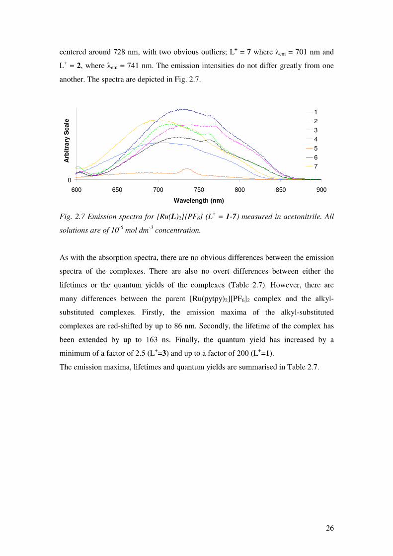
centered around 728 nm, with two obvious outliers; L+ = 7 where λem = 701 nm and

L+ = 2, where λem = 741 nm. The emission intensities do not differ greatly from one

another. The spectra are depicted in Fig. 2.7.

0

600 650 700 750 800 850 900

Wavelength (nm)

Arb

itra

ry S

cale

1

2

3

4

5

6

7

Fig. 2.7 Emission spectra for [Ru(L)2][PF6] (L+ = 1-7) measured in acetonitrile. All

solutions are of 10-6 mol dm-3 concentration.

As with the absorption spectra, there are no obvious differences between the emission

spectra of the complexes. There are also no overt differences between either the

lifetimes or the quantum yields of the complexes (Table 2.7). However, there are

many differences between the parent [Ru(pytpy)2][PF6]2 complex and the alkyl-

substituted complexes. Firstly, the emission maxima of the alkyl-substituted

complexes are red-shifted by up to 86 nm. Secondly, the lifetime of the complex has

been extended by up to 163 ns. Finally, the quantum yield has increased by a

minimum of a factor of 2.5 (L+=3) and up to a factor of 200 (L+=1).

The emission maxima, lifetimes and quantum yields are summarised in Table 2.7.

27

Complex Emission

Max (nm)

τ (ns)

Quantum

Yield (%)

(+/- 0.1%)

Ru(pytpy)2][PF6]225 655 3 0.04

[Ru(1)2][PF6]4 728 160a 0.73

[Ru(2)2][PF6]4 741 115a 0.38

[Ru(3)2][PF6]4 730 105a 0.01

[Ru(4)2][PF6]4 715 162a 0.35

[Ru(5)2][PF6]4 703 129a 0.05

[Ru(6)2][PF6]4 727 145a 0.45

[Ru(7)2][PF6]4 701 166a 0.44

Table 2.7 A summary of the photophysical properties of Ru(II) complexes with ligands

1-7, recorded in MeCN, a means the error is +/- 15 ns.

2.3.6 Electrochemistry

Cyclic voltammetry was used to examine the oxidation and reduction potentials of

each complex. Oxidation of the complex is the removal of an electron from the

highest occupied molecular orbital (HOMO). Reduction is the insertion of an electron

into the lowest unoccupied molecular orbital (LUMO) of the complex. For the

complex to do work, such as water splitting, the oxidation potential needs to be

appropriate; high enough to be above the oxidation potential of water but not so high

that oxidation of the complex is impossible.

The measurements were carried out in an MeCN solution of the complex using 0.1M

TBAPF6 as the supporting electrolyte. Ferrocene was added at the end of each

measurement as a reference. A square wave voltammagram was also measured as a

‘check’; data are not shown.

For all complexes a reversible one-electron oxidation was observed around 1.0 V (vs

Fc/Fc+), which is attributed to the oxidation of RuII to RuIII. Two reversible one-

electron ligand-centred reductions around -1.05 V and -1.45 V (vs Fc/Fc+), were also

observed for all complexes. The two reductions are attributed to the injection of an

electron into an unoccupied ligand π* orbital, to form a radical anion.

Fig. 2.8 depicts a representative cyclic voltammagram; [Ru(1)2][PF6]4.

28

-1.0E-04

-5.0E-05

0.0E+00

5.0E-05

1.0E-04

-3.0 -2.5 -2.0 -1.5 -1.0 -0.5 0.0 0.5 1.0 1.5

Voltage (V)

Cu

rre

nt

(A)

Fig. 2.8 Cyclic Voltammagram for [Ru(1)2][PF6]4 (MeCN, 0.1M TBAPF6, internal

reference; ferrocene).

The data for all of the complexes are summarised in Table 2.8. Further ligand-centred

reductions are observed for each complex, around -1.7 V, but in the case of L+ = 3 this

reduction is irreversible and in the cases of L+ = 5, 7 the reduction is quasi-reversible.

For complex L+ = 1 (Fig. 2.8) the asymmetry of the reduction peak at -1.0 V suggests

the possibility of two reduction processes at close potentials. For complexes L+ = 3, 5

and 7 a further reduction around -2.0 V is observed and this is irreversible in all cases.

29

Complex Ru2+/Ru3+

(V)

[Ru(pytpy)2][PF6]2 +0.95 -1.54 -1.80

[Ru(1)2][PF6]4 +1.07/

+0.96

-0.98/

-1.17

-1.45/

-1.58

-1.68/

-1.81

[Ru(2)2][PF6]4 +1.06/

+0.96

-0.97/

-1.13

-1.44/

-1.56

-1.67/

-1.79

[Ru(3)2][PF6]4 +1.12/

+0.98

-1.00/

-1.20

-1.30/

-1.49

-1.69irr -2.22irr

[Ru(4)2][PF6]4 +1.05/

+0.95

-1.04/

-1.23

-1.52/

-1.62

-1.73/

-1.84

[Ru(5)2][PF6]4 +1.08/

+0.96

-0.87/

-1.04

-1.35/

-1.46

-1.56/

-1.71qr

-1.99irr

[Ru(6)2][PF6]4 +1.07/

+0.97

-1.03/

-1.17

-1.50/

-1.57

-1.71/

-1.80

[Ru(7)2][PF6]4 +1.06/

0.94

-1.05/

-1.21

-1.51/

-1.61

-1.73/

-1.84qr

-1.94irr

Table 2.8 A summary of the redox potentials for Ru(II) complexes with ligands 1-7.

Measurements carried out in MeCN, using 0.1M TBAPF6 as the electrolyte and

referenced to Fc/Fc+. qrQuasi-reversible; irrIrreversible

The alkyl-substituted complexes have a higher Ru(II)/Ru(III) redox potential than that

of the parent [Ru(pytpy)2][PF6]2 complex. This means that abstraction of an electron

from the HOMO of the alkylated complexes requires more energy than for the parent

complex. The negligible change in redox potentials between complexes complements

the photophysical data leading to the conclusion that changing the substituent has a

negligible effect on the Ru(tpy)2 core.

Ligand centred reductions (V)

30

2.3.7 Crystal Structures

Crystal structures of the following complexes were obtained:

• [Ru(1)2][PF6]4•H2O

• [Ru(3)2][PF6]4

• [Ru(4)2][PF6]4•H2O

• [Ru(6)2][PF6]4•2MeCN

• [Ru(7)2][PF6]4

Red blocks of [Ru(1)2][PF6]4•H2O were grown by slow evaporation of an acetonitrile

solution of the complex and the structure confirmed benzylation at both terminal

pyridine rings. The crystal structure solves in the P -1 space group, with a poor R

factor of 15.0 %. The asymmetric unit contains 2 independent cations with 7 whole

PF6 counter-anions, 2 half PF6 counter-anions and two water molecules.

The structure of one of the [Ru(1)2]4+ cations is depicted in Fig. 2.9 and selected bond

lengths and angles are listed in the caption.

Fig. 2.9 Structure of one of the [Ru(1)2]4+ cations with ellipsoids plotted at 50%

probability and hydrogen atoms omitted for clarity. Selected bond parameters:

Ru1-N1 = 2.07 (1), Ru1-N2 = 1.97(1), Ru1-N3 = 2.06(1), Ru1-N5 = 2.07(1),

Ru1-N6 = 1.969(7), Ru1-N7 2.06 (1), N4-N21 = 1.50 (2), N8-C48 = 1.46(2) Å;

N2-Ru1-N1 = 79.5(4), N2-Ru1-N3 = 78.9 (4), N5-Ru1-N6 = 79.4(4),

N6-Ru1-N7 = 78.5(4)°.

Ru1

N1 N2

N4

N3

N5

N6

N7

N8

C21

C48

C5

C11

C38

31

As expected for a [Ru(X-tpy)2]n+ (X = any substituent) complex the ruthenium atom

coordinates two ligands through the nitrogen atoms of the terpyridine moieties. The

terpyridine ligands are almost orthogonal to one another; the angle between the planes

is 89.03º (plane 1: N1, C5, ring containing N2 and C11, N3, plane 2: N5, C32, ring

containing N6 and C38, N7). The Ncentral-Ru-Ncentral vector was expected to be linear,

with an N4-Ru1-N8 angle of 180º, however, a bowing of the [Ru(1)2]4+ cation is

observed. This bowing is also present for [Ru(pytpy)2][PF6][NO3]•DMSO26 and

[Ru(pytpy)][PF6][NO3]27 (N4-Ru1-N8 angles are 169.11(4)º and 176.03(7)º,

respectively). Compared to these two complexes the bowing of [Ru(1)2][PF6]4 is

much greater (163.4º), which is probably due to the effect that the benzyl substituent

has on the packing (see later). The bond lengths and angles within the Ru-tpy unit are

unexceptional. The N4-C21 and N8-C48 bond lengths of 1.50(2) and 1.46(2) Å,

respectively, are consistent with single bonds between each pendant pyridine N atom

and the benzyl group.

Two independent cations reside in the asymmetric unit. The cations differ most

greatly in the orientation of the benzyl substituents. For comparison, the two

complexes have been overlaid and are depicted in Fig. 2.10.

Fig. 2.10 An overlay of the two independent cations in the asymmetric unit, black dots

denote the centroids.

The core Ru(tpy)2 regions of the cations are similar. In one complex (blue) both of

the benzyl substituents are orientated in the same direction. In the other complex (red)

one benzyl substituent is almost orthogonal (angle between planes 86.8º) to the

terminal pyridyl moiety, to which it is attached. (Plane 1 is the terminal pyridine ring,

C21

• •

32

plane 2 is the benzyl ring.) The distance between the centroids of the two rings is

4.8Å and the centroid-C21-centroid angle is 111.3º. The other benzyl group is roughly

perpendicular to the terminal pyridyl group, with the angle between the planes of

74.8º. The distance between the two centroids is also 4.8Å, and the centroid-C48-

centroid angle, 111.5º, is effectively the same as for the previously described

substituent. The centroid to centroid bond lengths and angles are consistent with the

carbon atom being constrained to tetrahedral geometry by bonding to four different

groups. (Plane 1 is the terminal pyridine ring, plane 2 is the benzyl ring.)

The complexes pack with intermeshing benzyl groups. Within the crystal lattice there

are extensive short contacts between hydrogen atoms and fluorine atoms of the

hexafluorophosphate counter-anions (e.g. H4-F4 2.56Å).

Fig. 2.11 Packing of the cations in [Ru(1)2][PF6]4•H2O with the Ru(pytpy)2- core in

blue and the pendant benzyl groups in red.

33

The cations were expected to pack with two dimensional tpy embrace layers28-32 and

some intercalation of the cations can be observed (Fig 1.11 top). However, the benzyl

substituent distorts the tpy-tpy embrace by occupying the space between the tpy units,

forcing them apart (Fig. 2.11 bottom). This also prohibits π-stacking throughout the

lattice.

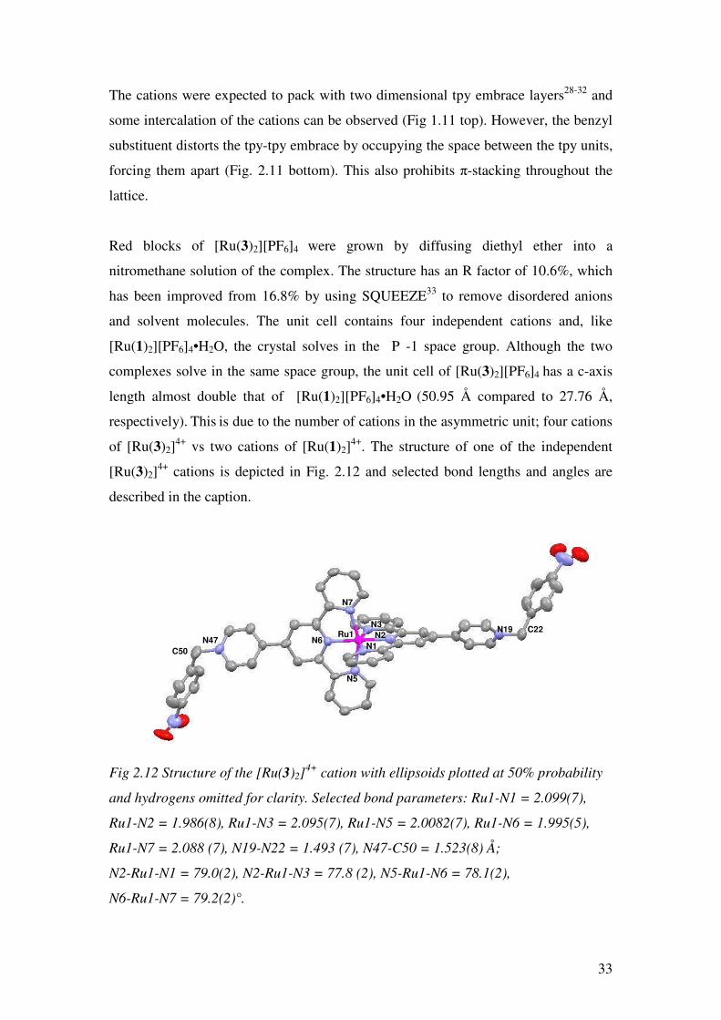
Red blocks of [Ru(3)2][PF6]4 were grown by diffusing diethyl ether into a

nitromethane solution of the complex. The structure has an R factor of 10.6%, which

has been improved from 16.8% by using SQUEEZE33 to remove disordered anions

and solvent molecules. The unit cell contains four independent cations and, like

[Ru(1)2][PF6]4•H2O, the crystal solves in the P -1 space group. Although the two

complexes solve in the same space group, the unit cell of [Ru(3)2][PF6]4 has a c-axis

length almost double that of [Ru(1)2][PF6]4•H2O (50.95 Å compared to 27.76 Å,

respectively). This is due to the number of cations in the asymmetric unit; four cations

of [Ru(3)2]4+ vs two cations of [Ru(1)2]

4+. The structure of one of the independent

[Ru(3)2]4+ cations is depicted in Fig. 2.12 and selected bond lengths and angles are

described in the caption.

Fig 2.12 Structure of the [Ru(3)2]4+ cation with ellipsoids plotted at 50% probability

and hydrogens omitted for clarity. Selected bond parameters: Ru1-N1 = 2.099(7),

Ru1-N2 = 1.986(8), Ru1-N3 = 2.095(7), Ru1-N5 = 2.0082(7), Ru1-N6 = 1.995(5),

Ru1-N7 = 2.088 (7), N19-N22 = 1.493 (7), N47-C50 = 1.523(8) Å;

N2-Ru1-N1 = 79.0(2), N2-Ru1-N3 = 77.8 (2), N5-Ru1-N6 = 78.1(2),

N6-Ru1-N7 = 79.2(2)°.

N1

N3

N5

N6

N7

N19

N47

C22

C50

Ru1 N2

34

Two ligands are coordinated to the ruthenium atom, resulting in an octahedral

geometry. The two terpyridines are close to orthogonal; the angle between the planes

is 89.7º. As for [Ru(1)2]4+ there is a bowing of the cation backbone away from

linearity but, by comparison, for [Ru(3)2]4+ this bowing is less pronounced

(N4-Ru1-N8 = 173.4º). The bond lengths and angles around the Ru(tpy)2 core are

unremarkable. The N19-C22 and N47-C50 bond lengths of 1.493(7) and 1.485(7) Å

respectively, are consistent with single bonds between the N atom of the pendant

pyridine and the nitrobenzyl substituent. These bond lengths are also very similar to

the analogous bonds in [Ru(1)2][PF6]4•H2O.

Fig. 2.13 Packing of the cations with the Ru(pytpy)2- core in blue and the pendant

nitrobenzyl groups in red.

Typical tpy-tpy embraces28-32 are observed in the packing of [Ru(3)2]4+, with both

face-to-face and edge-to-face interactions. The edge-to-face distances range from 2.35

to 2.93 Å and the face-to-face distances are longer, 3.61-3.85 Å. The majority of

nitrobenzyl subsituents pack orthogonally to the Ru(pytpy)2 core and, therefore, do

35

not disrupt the packing. Some π-stacking34 is observed between the nitrobenzyl

groups, centroid-centroid distance = 3.76 Å, (Fig 2.14). No π-stacking is observed

between the pyridylterpyridine units.

Fig. 2.14 π-stacking between the two benzyl rings of the nitrobenzyl subsituents

(benzyl rings depicted in purple, centroids in yellow).

Red needles of [Ru(4)2][PF6]4•H2O were grown by diffusing diethyl ether into an

acetone solution of the complex. The structure has a reasonable R factor of 6.6 % and

solves in the space group P 21/c. The asymmetric unit contains one [Ru(4)2]4+ cation,

four PF6- counter-anions and one water molecule. One ethyl group is disordered over

two positions and has been modelled over two sites with fractional occupancies of

0.76 and 0.24. All four PF6- counter-anions and the water molecule are disordered.

The two ligands coordinate orthogonally to the central ruthenium atom (angle

between the tpy planes is 87.8º) causing an octahedral geometry of the cation. There

is a slight bowing of the cation from linearity; N4-Ru1-N8 angle = 171.5º, more than

that of [Ru(3)2]4+ but less than that of [Ru(1)2]

4+. The bond lengths and angles are

standard for this type of complex. The N4-C21 and N8-C43 bond lengths are

consistent with analogous bond lengths for the aforementioned [Ru(L)2]4+ complexes.

36

Fig. 2.15 Structure of the [Ru(4)2]4+ cation with ellipsoids plotted at 50% probability

and hydrogens omitted for clarity. Ethyl groups shown in the major occupancy

position. Selected bond parameters: Ru1-N1 =2.076(4) , Ru1-N2 =1.981(3),

Ru1-N3 =2.088(4), Ru1-N5 =2.082(3), Ru1-N6 = 1.976(3), Ru1-N7=2.075(3),

N4-N21 = 1.49(2), N8-C43 = 1.486(7) Å; N2-Ru1-N1 = 79.4(1),

N2-Ru1-N3 = 78.4 (1), N5-Ru1-N6 = 78.7(1), N6-Ru1-N7 = 78.9(1)°.

Fig. 2.16 (left and centre) Packing of the cations. (right) Intermeshing of the ethyl

groups. Ru(pytpy)2-core in blue, pendant ethyl substituents in red.

The cations pack with typical tpy-tpy Dance embraces28-32. There are face-to-face and

edge-to-face interactions between the terpyridine moieties, uninterrupted by the ethyl

substituents. The ethyl groups are directed above and below the plane and are all

oriented in the same direction. There are also extensive CH…F packing interactions

throughout the lattice (e.g. H24-F31 2.64 Å).

N1

N3

N2

N5

N6

N7 N4

N8

C21

C43

Ru1

37

Small red blocks of [Ru(6)2][PF6]4 were grown by slow evaporation of an acetonitrile

solution of the complex. The structure solves in the Cc space group with a good

R factor of 4.7 %. The asymmetric unit contains one [Ru(6)]4+ cation, four PF6-

anions, one of which is disordered, two molecules of acetonitrile and one water

molecule. The structure of the [Ru(6)2]4+ cation is depicted below and selected bond

lengths and angles are listed in the caption.

Fig. 2.17 Structure of the [Ru(6)2]4+ cation with ellipsoids plotted at 50% probability

and hydrogens omitted for clarity. Allyl groups shown in the major occupancy

positions. Selected bond parameters: Ru1-N1 = 2.058 (2), Ru1-N2 = 1.981 (2),

Ru1-N3 = 2.067 (2), Ru1-N5 = 2.096(2), Ru1-N6 = 1.981(3), Ru1-N7 = 2.097(3),

N4-C21 = 1.57(1), C21-C22 = 1.50(2) , C22-C23 =1.13 (2), N8-C44 = 1.536(6),

C44-C45 = 1.471(7) , C45-C46 =1.28(1) Å ; N1-Ru1-N2 = 78.56 (9),

N2-Ru1-N3 = 78.93(9), N5-Ru1-N6 = 78.5(1), N6-Ru1-N7 = 78.9(1)°.

The two ligands are coordinated orthogonally to the central ruthenium atom and the

angle between the two terpyridine planes is 79.0º. The ligand is disordered, and the

fractional occupancies of the C21-C22-C23 allyl chain are 0.289 (4) and 0.711(4).

The occupancies of the C44-C45-C46 chain are 0.80 and 0.20. The structure confirms

successful alkylation at the pendant pyridyl moieties and the N4-C21 and C21-C22

bond lengths indicate single bonds. The C22-C23 and C45-C46 bond lengths are

shorter, 1.13(2) Å and 1.28(1) respectively, which are consistent with double bonds

between the two carbon atoms. The ruthenium – nitrogen bond lengths are typical of

Ru(tpy)2- based complexes.

N1

N3

N2

N8 C44

N4

Ru1

C45

C46 N7

C21

C22

C23

N6

N5

38

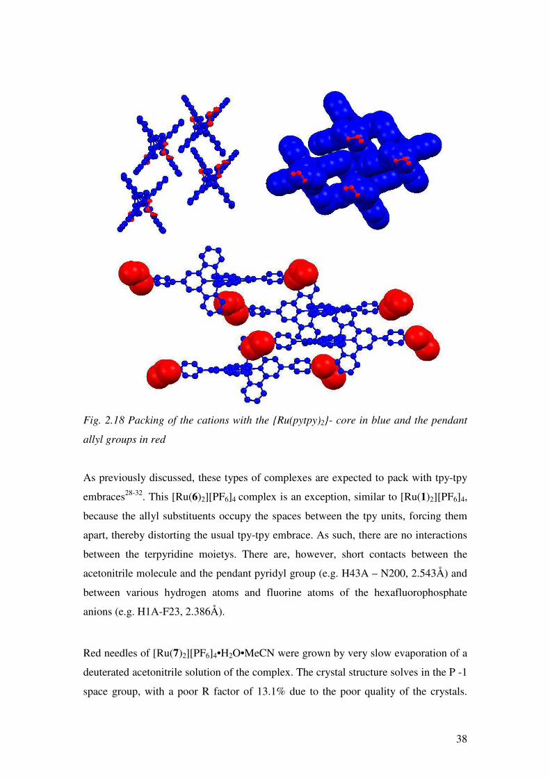
Fig. 2.18 Packing of the cations with the Ru(pytpy)2- core in blue and the pendant

allyl groups in red

As previously discussed, these types of complexes are expected to pack with tpy-tpy

embraces28-32. This [Ru(6)2][PF6]4 complex is an exception, similar to [Ru(1)2][PF6]4,

because the allyl substituents occupy the spaces between the tpy units, forcing them

apart, thereby distorting the usual tpy-tpy embrace. As such, there are no interactions

between the terpyridine moietys. There are, however, short contacts between the

acetonitrile molecule and the pendant pyridyl group (e.g. H43A – N200, 2.543Å) and

between various hydrogen atoms and fluorine atoms of the hexafluorophosphate

anions (e.g. H1A-F23, 2.386Å).

Red needles of [Ru(7)2][PF6]4•H2O•MeCN were grown by very slow evaporation of a

deuterated acetonitrile solution of the complex. The crystal structure solves in the P -1

space group, with a poor R factor of 13.1% due to the poor quality of the crystals.

39

The asymmetric unit contains one cation, two ordered PF6- anions, two disordered

PF6- counter-anions, one acetonitrile molecule and one water molecule.

The unit cell has similar dimensions to that of [Ru(1)2][PF6]4. It is shorter in a, 8.7018

(7) Å, compared to 13.488 (3) Å, and b, 12.5549 (10) Å compared to 16.934 (3) Å

and slightly longer in c, 30.067 (3) Å compared to 27.758 (6) Å. The decrease in the

length of the a and b axes is due to the asymmetric unit containing one cation for

[Ru(7)2][PF6]4•H2O•MeCN compared to two for [Ru(1)2][PF6]4•H2O. The structure of

the [Ru(7)2]4+ cation is depicted in Fig 2.19 and selected bond lengths and angles are

listed in the caption. One of the terminal pyridyl moieties is disordered and modelled

over two positions, with fractional occupancies of 0.43 and 0.57, only the major

occupancies shown in Fig. 2.19.

Fig. 2.19. Structure of the [Ru(7)2]4+ cation with ellipsoids plotted at 50% probability

and hydrogens omitted for clarity. Selected bond parameters: Ru1-N1 = 2.085 (7),

Ru1-N2 = 1.975 (7), Ru1-N3 = 2.062 (7), Ru1-N5 = 2.069 (7), Ru1-N6 = 1.960 (6),

Ru1-N7 = 2.078 (7) N4-C21 = 1.50 (1), N8-C49 = 1.46 (3) Å; N2-Ru1-N1 = 78.5 (3),

N2-Ru1-N3 = 78.7 (3), N5-Ru1-N6 = 77.5 (3), N6-Ru1-N7 = 79.4 (3)°.

The bond lengths and angles of the cation are unexceptional and the two ligands

coordinate to the central ruthenium atom in the expected, orthogonal, manner. The

angle between the two terpyridine planes is 89.6º. The C-C bond lengths of the octyl

chain are all typical of single bonds and are in the range of 1.47(1) to 1.57(1) Å, with

an average C-C bond length of 1.52 Å. The bowing of the cation away from linearity

(N4-Ru1-N8 = 170.5º) is of a similar magnitude to that observed for [Ru(4)2][PF6]4.

N3

N1

N2

N5

N6

N7 N4

C21

N8

C49 Ru1

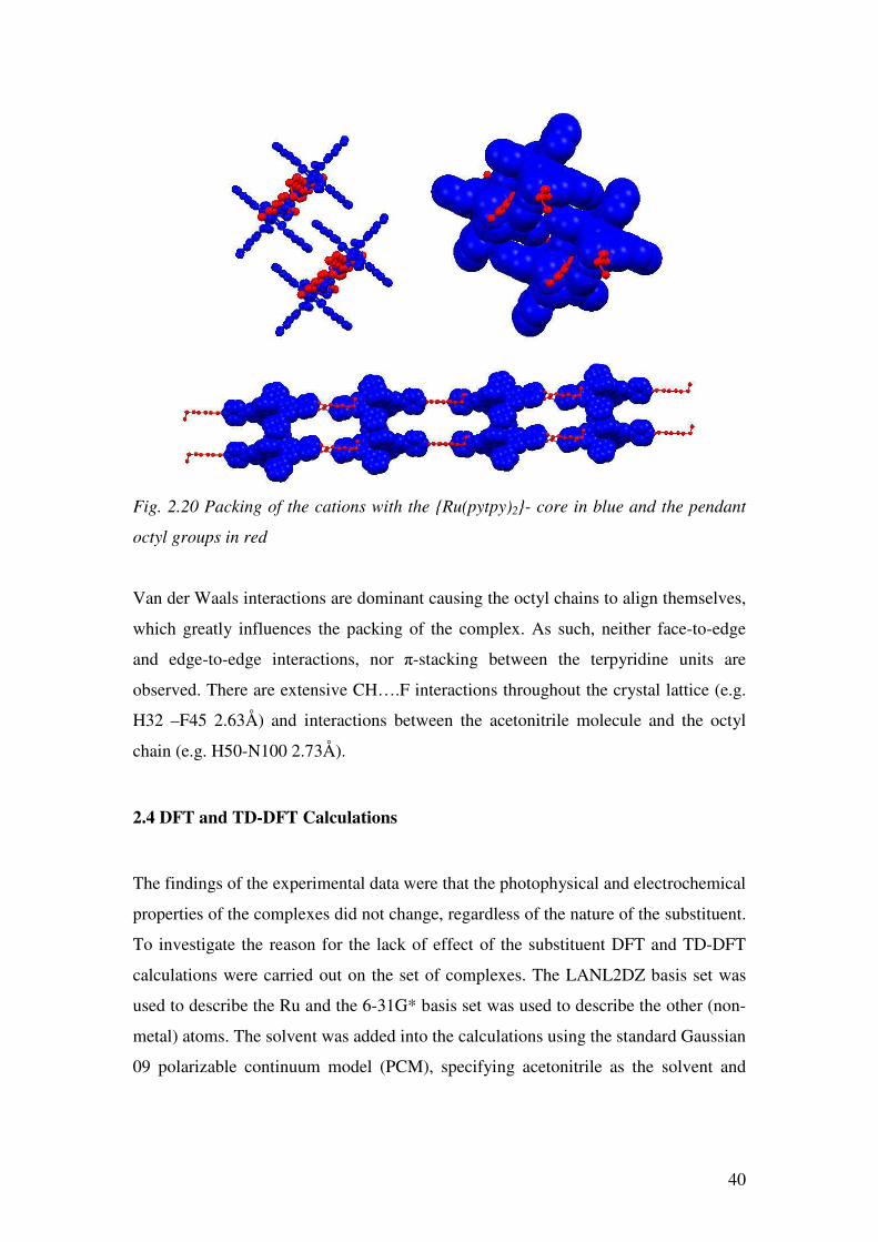
40

Fig. 2.20 Packing of the cations with the Ru(pytpy)2- core in blue and the pendant

octyl groups in red

Van der Waals interactions are dominant causing the octyl chains to align themselves,

which greatly influences the packing of the complex. As such, neither face-to-edge

and edge-to-edge interactions, nor π-stacking between the terpyridine units are

observed. There are extensive CH….F interactions throughout the crystal lattice (e.g.

H32 –F45 2.63Å) and interactions between the acetonitrile molecule and the octyl

chain (e.g. H50-N100 2.73Å).

2.4 DFT and TD-DFT Calculations

The findings of the experimental data were that the photophysical and electrochemical

properties of the complexes did not change, regardless of the nature of the substituent.

To investigate the reason for the lack of effect of the substituent DFT and TD-DFT

calculations were carried out on the set of complexes. The LANL2DZ basis set was

used to describe the Ru and the 6-31G* basis set was used to describe the other (non-

metal) atoms. The solvent was added into the calculations using the standard Gaussian

09 polarizable continuum model (PCM), specifying acetonitrile as the solvent and

41

predicted TD-DFT transitions were calculated using the ab initio, B3LYP method.

(see experimental section for more details.)

To validate the calculations a comparison between the calculated bond lengths and the

bond lengths determined by crystallography was done for three of the cations. These

were [Ru(1)2]4+, [Ru(3)2]

4+ and [Ru(4)2]

4+ although less can be learnt by comparing

the data for [Ru(3)2]4+ as the crystallographic R factor was so poor. The comparison is

tabulated in Table 2.9 and the values of x and y are given in the table description.

(x and y refer to the numbers of the terminal pendant pyridyl nitrogens as defined in

the crystallography section of this chapter. §Section 2.3.7.)

Parameter L+ = 1

(DFT)

L+= 1

(exp)

L+ = 3

(DFT)

L+ = 3

(exp)

L+ = 4

(DFT)

L+ = 4

(exp)

Ru1-N1 2.129 2.099(7) 2.127 2.099(7) 2.128 2.076(3)

Ru1-N2 2.017 1.986(8) 2.015 1.986(8) 2.015 1.981(3)

Ru1-N3 2.127 2.095(7) 2.128 2.095(7) 2.128 2.088(3)

Ru1-N5 2.127 2.0082(7) 2.126 2.0082(7) 2.128 2.082(4)

Ru1-N6 2.016 1.995(5) 2.015 1.995(5) 2.015 1.976(3)

Ru1-N7 2.129 2.088(7) 2.128 2.088(7) 2.128 2.075(4)

N4-C21 1.518 1.50(2) 1.497 1.501(7) 1.494 1.487(19)

Nx-Cy 1.518 1.46(2) 1.500 1.501(7) 1.494 1.486(6)

N2-Ru1-N1 78.27 79.5(4) 78.31 77.8(2) 78.33 79.37(14)

N2-Ru1-N3 78.24 78.9(4) 78.30 79.3(2) 78.30 78.44(14)

N5-Ru1-N6 78.30 79.4(4) 78.34 78.8(2) 78.33 78.70(14)

N6-Ru1-N7 78.27 78.5(4) 78.24 78.1(2) 78.30 78.95(14)

Table 2.9 Comparison between calculated and X-ray crystal structure determined

bond lengths and angles for complexes [Ru(L)2]4+ where L+ =1 (x=8, y=48), 3 (x=47,

y=50), 4 (x=8, y=43). Atom numbering corresponds to figs 2.9, 2.13 and 2.16.

The agreement between the calculated and experimental structures is good. The

calculated bond lengths are generally slightly over-estimated by <0.1Å and the

calculated bond angles agree with the crystal structure data to within 1.1°. The

calculations predict that the substituent at the terminal pyridyl moiety will have a

small effect on the C-N bond length but this is not reproduced experimentally. As the

42

agreement between the calculated and experimental data is good the level of

calculation chosen is correct. The energy and structure of the complexes were then

minimised again in the presence of the solvent and pictures of the highest lying

occupied and lowest lying unoccupied molecular orbitals were generated using the

program Molekel35.

The lowest lying unoccupied molecular orbitals are purely ligand based and the

highest lying occupied molecular orbitals are metal based. The localisation of the

molecular orbitals on each complex explained the lack of difference in the

photophysical and electrochemical properties in the series. The HOMO and

(HOMO−1) are predominantly metal based and do not change from complex to

complex and, therefore, cannot effect a change between the properties of the

complexes. Furthermore, the LUMO and (LUMO+1) do not extend beyond the

terminal pyridyl moiety, due to the break in conjugation caused by the –CH2- group.

As neither the metal orbitals nor the ligand orbitals change with substituent the MLCT

would not be expected to change either. Molecular orbitals of representative

complexes are depicted in Figs. 2.21 and 2.22.

Fig. 2.21 Top left, [Ru(3)2]4+ (HOMO−1), top right, [Ru(3)2]

4+ HOMO

Bottom left [Ru(6)2]4+ (HOMO−1), bottom right, [Ru(6)2]

4+ HOMO

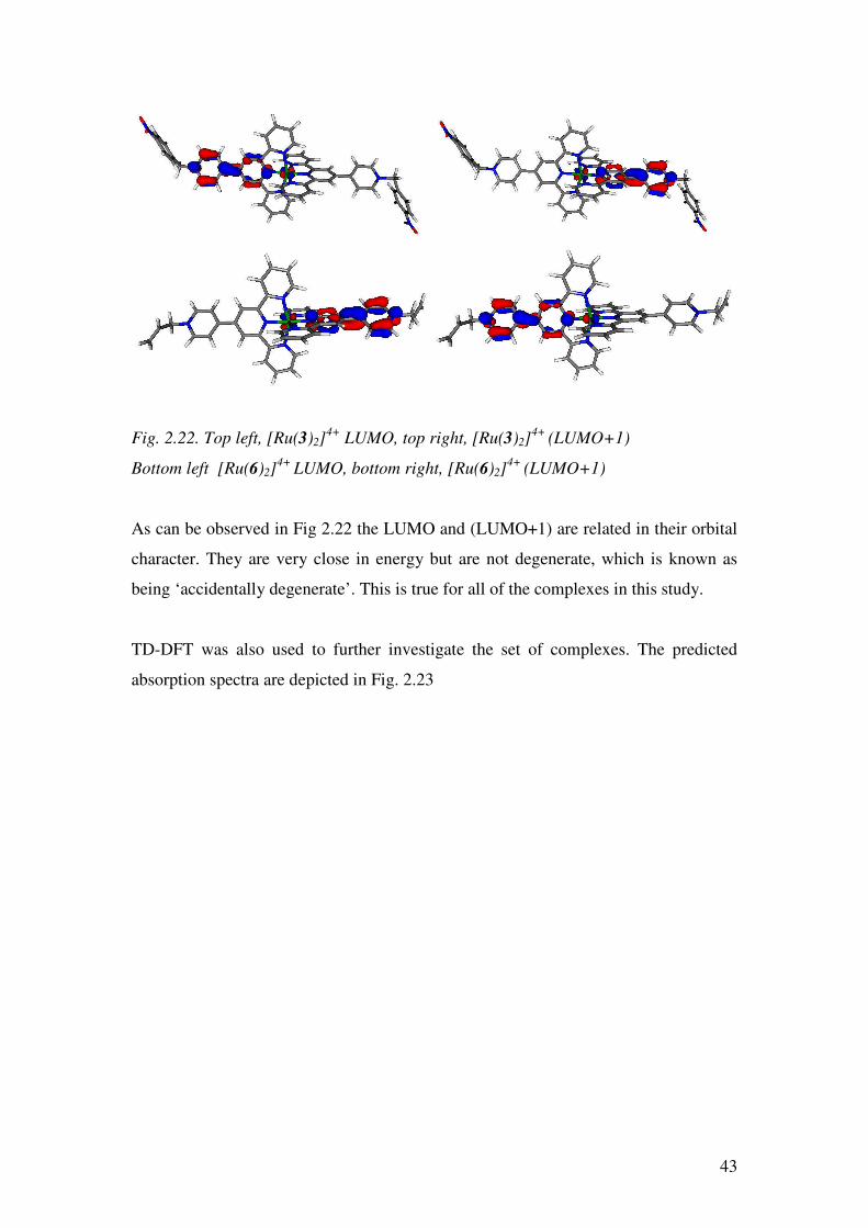
43

Fig. 2.22. Top left, [Ru(3)2]4+ LUMO, top right, [Ru(3)2]

4+ (LUMO+1)

Bottom left [Ru(6)2]4+ LUMO, bottom right, [Ru(6)2]

4+ (LUMO+1)

As can be observed in Fig 2.22 the LUMO and (LUMO+1) are related in their orbital

character. They are very close in energy but are not degenerate, which is known as

being ‘accidentally degenerate’. This is true for all of the complexes in this study.

TD-DFT was also used to further investigate the set of complexes. The predicted

absorption spectra are depicted in Fig. 2.23

44

0

350 400 450 500 550 600 650

Wavelength (nm)

Ab

s.

/ A

rbit

rary

Scale

[Ru(pytpy)2]2+

[Ru(1)2]4+

[Ru(2)2]4+

[Ru(3)2]4+

[Ru(4)2]4+

[Ru(5)2]4+

[Ru(6)2]4+

[Ru(7)2]4+

Fig. 2.23 The predicted absorption spectra for [Ru(pytpy)2][PF6]2 and[Ru(L)2][PF6]4

(L+=1-7).

The calculated spectra accurately reproduce the red shift upon alkylation of the parent

[Ru(pytpy)2]2+ complex. The calculations predict one major peak around 500 nm

(depending on substituent) and a shoulder at ~450 nm. The predicted shoulder at

~450 nm explains the non-gaussian shaped MLCT peak observed experimentally. The

calculations do not reproduce λmax exactly but the difference between the

experimental and calculated values is a maximum of 44 nm. This is acceptable

considering previously published calculations on ruthenium polypyridyl complexes

where the predicted experimental and calculated UV-vis spectra differ by up to

100 nm15-17, 22. The agreement between the spectra is depicted more clearly in

Fig. 2.24, which contains the calculated and experimental UV-vis spectra of

[Ru(4)2]4+.

45

0

350 400 450 500 550 600

Wavelength (nm)

Ab

s. / A

rbit

rary

Sc

ale

Calculated

Experimental

Fig. 2.24 Comparison of calculated and experimental MLCT band of complex

[Ru(4)2]4+

The transitions which contribute to the MLCT band, for all complexes, are

summarised (Table 2.10).

46

Complex λmax / nm Orbital Contributions

[Ru(1)2]4+ 478.4 48% (LUMO+1)←(HOMO−1)

47% LUMO←(HOMO−2)

[Ru(2)2]4+ 486.3 38% LUMO←(HOMO-2)

34% (LUMO+1)←(HOMO−1)

13% LUMO←(HOMO−1)

10% (LUMO+1)←(HOMO−2)

[Ru(3)2]4+ 488.3 38% LUMO←(HOMO−2)

34% (LUMO+1)←(HOMO−1)

13% LUMO←(HOMO−1)

10% (LUMO+1)←(HOMO−2)

[Ru(4)2]4+ 478.8 48% (LUMO+1)←(HOMO−1)

47% LUMO←(HOMO−2)

[Ru(5)2]4+ 504.6 46% LUMO←(HOMO−2)

45% (LUMO+1)←(HOMO−1)

[Ru(6)2]4+ 481.6 36% LUMO←(HOMO−1)

31% (LUMO+1)←(HOMO−2)

14% LUMO←(HOMO−2)

13% (LUMO+1)←(HOMO−1)

[Ru(7)2]4+ 480.9 53% LUMO←(HOMO−1)

38% (LUMO+1)←(HOMO−2)

Table 2.10 A summary of the transitions making up the MLCT band for all complexes.

2.5 Conclusion

Functionalisation of the previously known [Ru(pytpy)2][PF6]2 complex with a variety

of n-alkyl and n-aryl substituents resulted in complexes with red-shifted MLCT and

emission bands and higher oxidation potentials, when compared to the parent

complex. The type of substituent had a negligible effect on the photophysical and

electrochemical properties of the molecule and this was explored using DFT. The

DFT lead to the conclusion that the –CH2- bridge between the pendant pyridyl ring

and the substituent broke the π-conjugation system. These complexes could have

application as water oxidation catalysts, which is discussed in the next chapter.

47

2.6 Experimental

General Synthesis of [Ru(L)2][PF6]4:

[Ru(pytpy)2][PF6]2 and the appropriate alkylating reagent (120 eq.) were dissolved in

acetonitrile (50 cm3) and refluxed at 90 ºC for between 3 and 72 hours. The reaction

was monitored by spot TLC. The volume of solvent was then reduced to c.a. 5 cm3

and the complex was purified using column chromatography (SiO2, see text for

eluent). Acetonitrile was removed under reduced pressure. [NH4][PF6] was added to

precipitate [Ru(L)2][PF6]4. The salt was collected on celite, washed with copious

amounts of water, EtOH and Et2O. It was then redissolved in MeCN, dried in vacuo

and the product was isolated as a red powder.

The eluents are defined as follows:

A Sol = 7:1:0.5 MeCN: H2O: sat. KNO3

B Sol = 7:2:2 MeCN: H2O: sat. KNO3

C Sol = 10:0.5:1.5 MeCN: H2O: sat. KNO3

[Ru(1)2][PF6]4

Reaction time: 12 hours

Column Eluent: B Sol (Rf = 0.33)

Yield: 153.3 mg, 69.7 % (starting with mg [Ru(pytpy)2][PF6]2)

1H NMR: (500 MHz, CD3CN, 25ºC, TMS) δ/ppm: 9.12 (4H, s, B

3),

9.08 (4H, d, J = 6.5 Hz, C2), 8.75 (4H, d, J = 6.6 Hz, C3), 8.68 (4H, d, J = 8.1 Hz, A3),

8.00 (4H, t, J = 7.9Hz, A4) 7.59 (10H, m, D), 7.42 (4H, d, J = 5.4 Hz, A

6),

7.23 (4H, t, J = 7.5Hz, A5), 5.89 (4H, s, a); 13C NMR: (126 MHz, CD3CN, 25ºC, TMS) δ/ppm: 158.24 (A2), 156.82 (B2), 154.00

(C4), 153.55 (A6), 146.28 (C2), 139.49 (A4), 133.77 (D), 130.58 (D), 130.29 (D1),

128.91 (A5), 127.63 (C3), 125.95 (A3), 123.25 (B3), 65.27 (a);

Found: C, 42.29; H, 3.00; N, 7.45; C54H42F24N8P4Ru.3H2O

requires C, 42.17; H, 3.15; N, 7.29;

MALDI-TOF (MeCN): m/z 1340.5 [M-PF6]+ (calc. 1339.2), 1196.3 [M-2PF6]

+

(calc. 1194.2), 1050.3 [M-3PF6]+ (calc. 1049.2)

48

[Ru(2)2][PF6]4

Reaction time: 12 hours

Column Eluent: B Sol, (Rf = 0.30)

Yield: 215.5 mg, 78.9 % (starting with 180 mg [Ru(pytpy)2][PF6]2)

1H NMR: (500 MHz, d6-DMSO, 25ºC, TMS) δ/ppm: 9.77 (4H, s, B3),

9.65 (4H, br d, J = 6.3 Hz, C2), 9.20 (4H, br d, J = 6.3 Hz, C3),

9.10 (4H, d, J = 8.1 Hz, A3), 8.17 (4H, t, J = 7.6 Hz, A4), 8.05 (4H, d, J = 8.2 Hz, D3),

7.82 (4H, d, J = 8.2 Hz, D2), 7.59 (4H, d, J = 5.3 Hz, A6), 7.34 (4H, m, A5),

6.13 (4H, s, a); 13C NMR: (126 MHz, d6-DMSO, 25ºC, TMS) δ/ppm: 157.4 (A2/B2), 155.4 (A2/B2),

152.5 (A6), 151.8 (C4), 146.1 (C2), 139.9 (B4), 139.6 (D1), 138.6 (A4), 133.2 (D3),

129.5 (D2), 128.1 (A5), 126.0 (C3), 125.2 (A3), 122.3 (B3), 118.4 (D4),

112.2 (D-C≡N), 62.54 (a);

Found: C, 41.64; H, 2.86; N, 8.86; C56H40F24N10P4Ru.4H2O

requires C, 41.88; H, 3.01; N, 8.72;

MALDI-TOF (MeCN): m/z 1245.0 [M-2PF6]+ (calc. 1244.2), 1100.0 [M-3PF6]

+

(calc. 1099.2)

[Ru(3)2][PF6]4

Reaction time: 12 hours

Column Eluent: A Sol, (Rf = 0.29)

Yield: 67.2 mg, 41.6 % (starting with 100 mg [Ru(pytpy)2][PF6]2)

1H NMR: (500 MHz, d6-DMSO, 25ºC, TMS) δ/ppm: 9.77 (4H, s, B

3),

9.66 (4H, d, J = 6.5 Hz, C2), 9.21 (4H, d, J = 6.6 Hz, C

3),

9.09 (4H, d, J = 8.1 Hz, A3 ), 8.41 (4H, d, J = 8.7 Hz, D2), 8.17 (4H, t, J = 7.7 Hz, A4),

7.90 (4H, d, J = 8.7 Hz, D2), 7.59 (4H, d, J = 5.5 Hz, A

6), 7.34 (4H, m, A5),

6.18 (4H, s, a); 13C NMR: (126 MHz, d6-DMSO, 25ºC, TMS) δ/ppm: 157.6 (A2/B2), 155.6 (A2/B2),

152.3 (A6), 152.0 (C4), 145.1 (C2), 141.6 (D1), 141.3 (D4), 129.8 (D2), 128.0 (A5),

125.8 (C3), 125.0 (A3), 124.2 (D3), 122.1 (B3), 62.0 (a);

49

Found: C, 39.62; H, 3.06; N, 8.65; C54H40 F24N10P4Ru.3H2O

requires C, 39.84; H, 2.85; N, 8.60.

MALDI-TOF (MeCN): m/z 1431.7 [M-PF6]+ (calc. 1429.1), 1285.6 [M-2PF6]

+

(calc. 1284.2), 1150.4 [Ru(3)(Hpytpy)(PF6)2]+ (calc. 1149.1),

1005.3 [Ru(3)(Hpytpy)(PF6)]+ (calc. 1004.2), 995.5 [M-4PF6]+ (calc. 994.2),

723.2 [Ru(pytpy)(Hpytpy)]+ (calc. 723.3).

[Ru(4)2][PF6]4

Reaction time: 72 hours

Column Eluent: B Sol, (Rf = 0.30)

Yield: 80.6 mg, 64.3 % (starting with 80 mg [Ru(pytpy)2][PF6]2)

1H NMR: (500 MHz, d6-DMSO, 25ºC, TMS) δ/ppm: 9.78 (4H, s, B

3),

9.52 (4H, d, J = 6.6 Hz, C2), 9.17 (4H, d, J = 6.6 Hz, C3), 9.12 (4H, d, J = 8.1 Hz, A3),

8.17 (4H, t, J = 7.7 Hz, A4), 7.58 (4H, d, J = 5.4 Hz, A6), 7.33 (4H, t, J = 6.5 Hz, A5),

4.80 (4H, m, a), 1.73 (6H, t, J = 7.3 Hz, b); 13C NMR: (126 MHz, d6-DMSO, 25ºC, TMS) δ/ppm: 157.6 (A2/B2), 155.6 (A2/B2),

152.6 (A6), 150.8 (C4), 145.4 (C2), 140.0 (B4), 138.5 (A4), 128.0 (A5), 125.2 (C3),

125.1 (A3), 122.0 (B3), 56.2 (a), 16.0 (b);

Found C, 36.96; H, 2.75; N, 8.07; C44H38F24N8P4Ru.3H2O

requires C, 37.38; H, 3.14; N, 7.93;

MALDI-TOF (MeCN): m/z 1216.8 [M-PF6]+ (calc. 1215.1), 1071.6 [M-2PF6]

+

(calc. 1070.2), 926.8 [M-3PF6]+ (calc. 925.2), 782.1 [M-4PF6]

+ (calc. 780.2)

[Ru(5)2][PF6]4

Reaction time: 12 hours

Column Eluent: B Sol, (Rf = 0.54)

Yield: 67.3 mg, 61.6 % (starting with 100 mg [Ru(pytpy)2][PF6]2)

50

1H NMR: (500 MHz, d6-DMSO, 25ºC, TMS) δ/ppm: 9.80 (4H, s, B3),

9.61 (4H, d, J = 6.5 Hz, C2), 9.25 (4H, d, J = 6.5 Hz, C3), 9.12 (4H, d, J = 8.1 Hz, A3),

8.17 (4H, t, J = 7.7 Hz, A4)7.58 (4H, d, J = 5.4 Hz, A6) 7.33 (4H, t, J = 6.5 Hz, A5),

6.08 (4H, s, a); 13C NMR: (126 MHz, d6-DMSO, 25ºC, TMS) δ/ppm: 157.4 (A2/B2), 155.5 (A2/B2),

152.5 (A6+C4), 146.4 (C2), 139.5 (B4), 138.6 (A4), 128.1 (A5), 125.4 (C3), 125.2 (A3),

122.2 (B3), 114.3 (C≡N), 47.6 (a);

Found: C, 36.35; H, 2.55; N, 9.84, C44H32F24N10P4Ru.4H2O

requires C, 36.35; H, 2.77; N, 9.63;

MALDI-TOF (MeCN): m/z 1092.4 [M-2PF6]+ (calc. 1092.1), 947.4 [M-3PF6]

+

(calc. 947.2), 908.6 [Ru(5)(Hpytpy)(PF6)]+ (calc. 908.1), 869.3 [Ru(Hpytpy)2(PF6)]

+

(calc. 869.1)

[Ru(6)2][PF6]4

Reaction time: 4 hours

Column Eluent: B Sol, (Rf = 0.20)

Yield: 100.4 mg, 73.2 % (starting with 100 mg [Ru(pytpy)2][PF6]2)

1H NMR: (500 MHz, d6-DMSO, 25ºC, TMS) δ/ppm: 9.79 (4H, s, B

3),

9.48 (4H, d, J = 6.7 Hz, C2), 9.19 (4H, d, J = 6.7 Hz, C3), 9.12 (4H, d, J = 8.2 Hz, A3),

8.17 (4H, t, J = 7.8 Hz, A4), 7.58 (4H, d, J = 5.5 Hz, A6), 7.33 (4H, t, J = 6.8 Hz, A5),

6.35 (2H, ddt, b), 5.59 (2H, d, J = 10.2 Hz, c1), 5.51 (2H, d, J = 17.2 Hz, c2),

5.43 (4H, d, J = 5.9 Hz, a); 13C NMR: (126 MHz, d6-DMSO, 25ºC, TMS) δ/ppm: 157.4 (A2/B2), 155.6 (A2/B2),

152.5 (A6), 151.3 (C4), 145.7 (C2), 139.9 (B4), 138.5 (A4), 131.5 (b), 128.0 (A5),

125.3 (C3), 125.1 (A3), 122.1 (B3), 121.6 (c), 62.1 (a);

Found: C, 38.68; H, 2.92; N, 8.44; C46H38F24N8P4Ru.2H2O

requires C, 38.91; H, 2.98; N, 8.44;

MALDI-TOF (MeCN): m/z 1240.7 [M-PF6]+ (calc. 1239.1), 1093.7 [M-2PF6]

+ (calc.

1094.2), 1055.7 [Ru(6)(Hpytpy)(PF6)2]+ (calc. 1054.1), 949.7 [M-3PF6]

+ (calc. 949.2),

910.6 [Ru(6)(Hpytpy)(PF6)]+ (calc. 909.2), 764.5 [Ru(6)(Hpytpy)]+ (calc. 764.2)

51

[Ru(7)2][PF6]4

Reaction time: 48 hours

Column Eluent: C Sol, (Rf = 0.36)

Yield: 121.7 mg, 38.4 % (starting with 200 mg [Ru(pytpy)2][PF6]2)

1H NMR: (500 MHz, CD3CN, 25ºC, TMS) δ/ppm: 9.14 (4H, s, B

3),

9.01 (4H, d, J = 6.6 Hz, C2), 8.77 (4H, d, J = 6.5 Hz C3), 8.70 (4H, d, J = 8.1 Hz, A3),

8.02 (4H, t, J = 7.9 Hz A4), 7.46 (4H, d, J = 5.5 Hz A

6), 7.25 (4H, m, A5),

4.69 (4H, t, J = 7.6 Hz, a), 2.13 (4H, s, b), 1.46 (8H, m, c+d), 1.35 (12H, m, e+f+g),

0.93 (6H, t, J = 6.7 Hz, h); 13C NMR: δC (126 MHz, CD3CN, 25ºC, TMS): 158.3 (A2/B2), 156.7 (A2/B2), 153.8

(A6), 155.6 (C4), 146.2 (C2), 142.0 (B4), 139.5 (A4), 128.9 (A5), 127.5 (C3), 126.0

(A3), 123.3 (B3), 62.7 (a), 32.3 (e/f/g), 31.7 (b), 29.5 (e/f/g), 29.4 (c/d), 26.6 (c/d),

23.25 (e/f/g), 14.4 (h);

Found: C, 42.28; H, 4.26; N, 7.24; C55H60F24N8P4Ru.3H2O

requires C, 42.15; H, 4.33; N, 7.08;

MALDI-TOF (MeCN): m/z 1384.1 [M-PF6]+ (calc. 1383.3), 1239.6 [M-2PF6]

+ (calc.

1238.3), 1094.5 [M-3PF6]+ (calc. 1093.4)

Computational Methods

Complexes [RuL2]4+ with L+ = 1-7 and [Ru(pytpy)2]

2+ were modelled using TD-DFT

implemented in the Gaussian 0936. Each complex was initially geometry-optimized

using the RHF method with a 3-21G basis set applied to non-metal

atoms, and the Los Alamos National Laboratory 2 double ζ (LANL2DZ) effective

core potential (ECP) used to describe the Ru2+ centre37. A double-zeta Ru basis set

associated with the LANL2DZ ECP was taken from the Basis Set Exchange38. The

ECP and basis set were defined explicitly in Gaussian 09 using the 'GEN' and

'Pseudo=Read' keywords. Frequency calculations were performed at this level of

theory for each complex to confirm the identification of a local minimum energy

structure. Further refinement of complex geometries followed using the B3LYP

hybrid density functional39 and a larger 6-31G(d) basis set for non-metal atoms, with

the same Ru2+ ECP/basis set combination as before. The Integral Equation Formalism

52

polarisable continuum model (PCM) was used during geometry optimization and for

subsequent TD-DFT calculations to describe solvation of each complex in MeCN to

more closely match the experimental conditions40-43. A similar level of calculation has

been applied to a series of [Ru(tpy)2]2+ complexes20, and the general reliability of the

LANL2DZ ECP combined with the B3LYP hybrid density functional for transition

metal complexes has been highlighted44. Predicted TD-DFT UV-VIS transitions were

calculated at the B3LYP level, and simulated spectra were generated from the

Gaussian 09 output using the GaussSum program45. Grids containing orbital densities

were written as 'cube' files by Gaussian 09, and were used to generate isodensity

surfaces for selected MOs using the Molekel35.

53

2.7 References

1. S. Campagna, F. Puntoriero, F. Nastasi, G. Bergamini, V. Balzani, V. Balzani and S. Campagna, Springer Berlin / Heidelberg, 2007, vol. 280, pp. 117-214.

2. A. J. Bard and M. A. Fox, Accounts Chem. Res., 1995, 28, 141-145. 3. A. Juris, V. Balzani, F. Barigelletti, S. Campagna, P. Belser and A. von

Zelewsky, Coord. Chem. Rev., 1988, 84, 85-277. 4. K. Zeitler, Angew. Chem. Int. Ed., 2009, 48, 9785-9789. 5. J. P. Sauvage, J. P. Collin, J. C. Chambron, S. Guillerez, C. Coudret, V.

Balzani, F. Barigelletti, L. De Cola and L. Flamigni, Chem. Rev., 1994, 94, 993-1019.

6. J. Wang and G. S. Hanan, Synlett, 2005, 2005, 1251,1254. 7. A. Amini, A. Harriman and A. Mayeux, Phys. Chem. Chem. Phys., 2004, 6,

1157-1164. 8. J. R. Winkler, T. L. Netzel, C. Creutz and N. Sutin, J. Am. Chem. Soc., 1987,

109, 2381-2392. 9. V. Balzani, S. Campagna, G. Denti, A. Juris, S. Serroni and M. Venturi,

Accounts Chem. Res., 1998, 31, 26-34. 10. E. A. Medlycott and G. S. Hanan, Coord. Chem. Rev., 2006, 250, 1763-1782. 11. J. A. Treadway, B. Loeb, R. Lopez, P. A. Anderson, F. R. Keene and T. J.

Meyer, Inorg. Chem., 1996, 35, 2242-2246. 12. E. A. Medlycott and G. S. Hanan, Chem. Soc. Rev., 2005, 34, 133-142. 13. M. Maestri, N. Armaroli, V. Balzani, E. C. Constable and A. M. W. C.

Thompson, Inorg. Chem., 1995, 34, 2759-2767. 14. J. E. Beves, E. L. Dunphy, E. C. Constable, C. E. Housecroft, C. J. Kepert, M.

Neuburger, D. J. Price and S. Schaffner, Dalton Trans., 2008, 386-396. 15. S. Fantacci, F. De Angelis and A. Selloni, J. Am. Chem. Soc., 2003, 125,

4381-4387. 16. M. K. Nazeeruddin, F. De Angelis, S. Fantacci, A. Selloni, G. Viscardi, P.

Liska, S. Ito, B. Takeru and M. Grätzel, J. Am. Chem. Soc., 2005, 127, 16835-16847.

17. M. K. Nazeeruddin, T. Bessho, L. Cevey, S. Ito, C. Klein, F. De Angelis, S. Fantacci, P. Comte, P. Liska, H. Imai and M. Graetzel, J. Photoch. Photobio. A, 2007, 185, 331-337.

18. Kohjiro Hara and H. Arakawa, in Handbook of Photovoltaic Science and Engineering, John Wiley & Sons, Ltd, 2003, pp. 663-700.

19. E. Jakubikova, W. Chen, D. M. Dattelbaum, F. N. Rein, R. C. Rocha, R. L. Martin and E. R. Batista, Inorg. Chem., 2009, 48, 10720-10725.

20. K. C. D. Robson, B. D. Koivisto, T. J. Gordon, T. Baumgartner and C. P. Berlinguette, Inorg. Chem., 2010, 49, 5335-5337.

21. R. Siebert, C. Hunger, J. Guthmuller, F. Schlütter, A. Winter, U. S. Schubert, L. González, B. Dietzek and J. Popp, J. Phys. Chem. C, 2011, 115, 12677-12688.

22. S. Kupfer, J. Guthmüller, M. Wächtler, S. Losse, S. Rau, B. Dietzek, J. Popp and L. González, Phys. Chem. Chem. Phys., 2011, 13, 15580-15588.

23. M. G. Lobello, S. Fantacci, A. Credi and F. De Angelis, Eur. J. Inorg. Chem., 2011, 2011, 1605-1613.

24. E. C. Constable and A. M. W. C. Thompson, J. Chem. Soc. Dalton Trans., 1994, 1409-1418.

54

25. E. L. Dunphy, PhD Thesis, University of Basel, 2009. 26. E. C. Constable, C. E. Housecroft, M. Neuburger, S. Schaffner and F. Schaper,

Inorg. Chem. Commun., 2006, 9, 616-619. 27. J. E. Beves, D. J. Bray, J. K. Clegg, E. C. Constable, C. E. Housecroft, K. A.

Jolliffe, C. J. Kepert, L. F. Lindoy, M. Neuburger, D. J. Price, S. Schaffner and F. Schaper, Inorg. Chim. Acta, 2008, 361, 2582-2590.

28. M. L. Scudder, H. A. Goodwin and I. G. Dance, New J. Chem., 1999, 23, 695-705.

29. J. McMurtrie and I. Dance, CrystEngComm, 2009, 11, 1141-1149. 30. J. McMurtrie and I. Dance, CrystEngComm, 2005, 7, 216-229. 31. J. McMurtrie and I. Dance, CrystEngComm, 2005, 7, 230-236. 32. I. Dance and M. Scudder, CrystEngComm, 2009, 11, 2233-2247. 33. A. L. Spek, Acta Crystallogr. D, 2009, 65, 148-155. 34. C. Janiak, J. Chem. Soc. Dalton Trans., 2000, 3885-3896. 35. U. Varetto, in Swiss National Computing Centre, Lugano, Switzerland, 2009. 36. M. J. Frisch, G. W. Trucks, H. B. Schlegel, G. E. Scuseria, M. A. Robb, J. R.

Cheeseman, G. Scalmani, V. Barone, B. Mennucci, G. A. Petersson, H. Nakatsuji, M. Caricato, X. Li, H. P. Hratchian, A. F. Izmaylov, J. Bloino, G. Zheng, J. L. Sonnenberg, M. Hada, M. Ehara, K. Toyota, R. Fukuda, J. Hasegawa, M. Ishida, T. Nakajima, Y. Honda, O. Kitao, H. Nakai, T. Vreven, J. J. A. Montgomery, J. E. Peralta, F. Ogliaro, M. Bearpark, J. J. Heyd, E. Brothers, K. N. Kudin, V. N. Staroverov, R. Kobayashi, J. Normand, K. Raghavachari, A. Rendell, J. C. Burant, S. S. Iyengar, J. Tomasi, M. Cossi, N. Rega, J. M. Millam, M. Klene, J. E. Knox, J. B. Cross, V. Bakken, C. Adamo, J. Jaramillo, R. Gomperts, R. E. Stratmann, O. Yazyev, A. J. Austin, R. Cammi, C. Pomelli, J. W. Ochterski, R. L. Martin, K. Morokuma, V. G. Zakrzewski, G. A. Voth, P. Salvador, J. J. Dannenberg, S. Dapprich, A. D. Daniels, Ö. Farkas, J. B. Foresman, J. V. Ortiz, J. Cioslowski and D. J. Fox, Gaussian Inc., Wallingford CT, 2009.

37. P. J. Hay and R. W. Willard, J. Chem. Phys., 1985, 82, 270-283. 38. K. L. Schuchardt, B. T. Didier, T. Elsethagen, L. Sun, V. Gurumoorthi, J.

Chase, J. Li and T. L. Windus, J. Chem. Inf. Comp. Sci., 2007, 47, 1045-1052. 39. C. Lee, W. Yang and R. G. Parr, Phys. Rev. B, 1988, 37, 785-789. 40. M. Benedetta and T. Jacopo, J. Chem. Phys., 1997, 106, 5151-5158. 41. E. Cancés, B. Mennucci and J. Tomasi, J. Chem. Phys., 1997, 107, 3032-3041. 42. B. Mennucci, E. Cancés and J. Tomasi, J. Phys. Chem. B, 1997, 101, 10506-

10517. 43. J. Tomasi, B. Mennucci and E. Cancés, J. Mol. Struct. Theochem, 1999, 464,

211-226. 44. Y. Yang, M. N. Weaver and K. M. Merz, J. Phys. Chem. A, 2009, 113, 9843-

9851. 45. N. M. O'Boyle, A. L. Tenderholt and K. M. Langner, J. Comp. Chem., 2008,

29, 839-845.

55

Chapter 3

Water soluble alkylated bis4'-(4-pyridyl)-2,2':6',2"-terpyridineruthenium(II)

complexes for application as water oxidation catalysts.

3.1 Introduction

In the search for new efficient fuel sources, scientists have looked to nature for

inspiration. Plants are capable of using the sun’s energy to convert CO2 into

carbohydrates and to split water into protons and oxygen via photosynthesis. The

oxidation of water to produce oxygen (Eqn. 3.1) is challenging as it is a four electron

process.

2H2O → 4H+ + 4e

- + O2 (Eqn. 3.1)

In plants, this process is carried out by photosystem II (Fig. 3.1). A manganese-oxygen

cluster [MnCa] oxidises water and passes electrons on to the amino acid tyrosine, which

in turn delivers them to P6801. P680 is a chlorophyll cluster that absorbs light at 680 nm

and acts as a photosensitiser2. These cascade reactions are a vital part of photosynthesis

and the structure of the oxygen evolving unit was found to be a cubane-like Mn3CaO4

cluster3, 4

.

Fig. 3.1 A representation of the processes involved in photosystem II in plants1.

To further understand this [MnCa] cluster, research has been carried out towards the

synthesis of mononuclear and polynuclear Mn clusters for testing as water oxidation

catalysts (WOCs)5-7

. In 1985 Tames et al. reported the first dinuclear Mn complex that

56

was active as a water oxidation catalyst5 and in 1999 Brudvig et al. reported the first

functional model for photosystem II8. This model was a dinuclear Mn complex with two

2,2ʹ:6ʹ,2ʺ-terpyridine ligands, two coordinated water molecules and two bridging-µ-oxido

ligands (Fig. 3.2).

Fig. 3.2 The cation in [H2O(tpy)MnIII

(O)2MnIV

(tpy)OH2][NO3]3, the first functional

model for photosystem II8.

Polypyridine ligands have also been used in ruthenium complexes which demonstrate

catalytic water oxidation ability. Whitten et al., in 1976, described the use of ruthenium

complexes with surfactant-functionalised bipyridine ligands (Fig. 3.3), which were

prepared as chloroform films, to oxidise water9.

Fig. 3.3 First reported water-splitting ruthenium complexes9.

57

Thereafter, little progress was made in the field until 2005 when Thummel et al. reported

three novel mononuclear ruthenium complexes which showed WOC activity10

. These

complexes contained polypyridyl ligands and a coordinated water molecule, and could

produce O2 with a turnover number (TON) of 260. TON is the number of moles of

substrate (in this case water) that one mole of catalyst can convert before becoming

inactive11

. Following this, many ruthenium-pyridyl complexes were reported and have

been the subject of recent reviews6, 7, 12, 13

.

In general, ruthenium complexes which are active as water oxidation catalysts consist of

the following: a polydentate (bis- to tetra-dentate) polypyridyl ligand, one or more

pyridine ligands and either a coordinated water molecule or a coordinated halide (Fig.

3.4)13

.

Fig. 3.4. A representative structure of a ruthenium-based water oxidation catalyst,

X = H2O, n = 2, X = Cl, Br, I, n = 1.

Many possible types of complexes are summarised in a recent paper by Thummel et al.14

where a family of 28 mononuclear Ru(II) complexes were synthesised and tested as

catalysts for water splitting. In this family of complexes the highest TON achieved was

1170, in 24 hours.

The reaction mechanism of water oxidation by ruthenium complexes of the afore-

mentioned type has been studied in detail by Meyer et al.15

. The mechanism has been

shown to be dependent on the ruthenium atom being able to coordinate a water molecule

and then achieve oxidation states of +4 and +5 by forming a Ru=O double bond (Fig.

3.5).

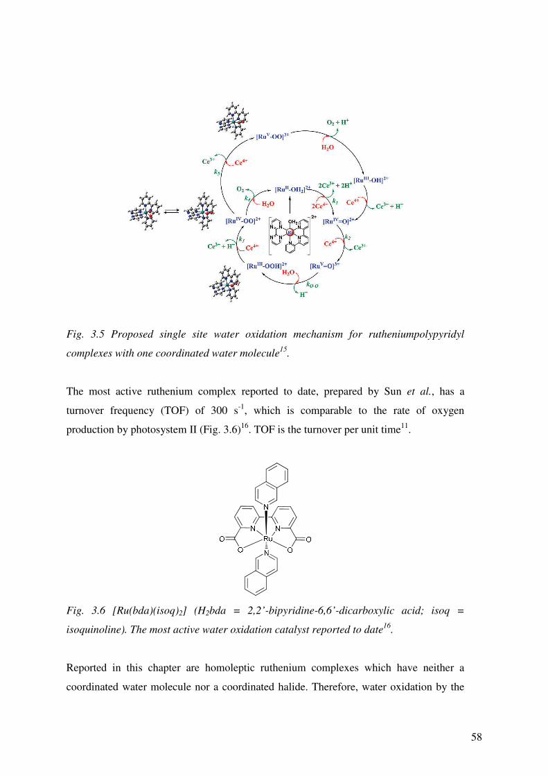
58

Fig. 3.5 Proposed single site water oxidation mechanism for rutheniumpolypyridyl

complexes with one coordinated water molecule15

.

The most active ruthenium complex reported to date, prepared by Sun et al., has a

turnover frequency (TOF) of 300 s-1

, which is comparable to the rate of oxygen

production by photosystem II (Fig. 3.6)16

. TOF is the turnover per unit time11

.

Fig. 3.6 [Ru(bda)(isoq)2] (H2bda = 2,2’-bipyridine-6,6’-dicarboxylic acid; isoq =

isoquinoline). The most active water oxidation catalyst reported to date16

.

Reported in this chapter are homoleptic ruthenium complexes which have neither a

coordinated water molecule nor a coordinated halide. Therefore, water oxidation by the

59

aforementioned mechanism is not possible. However, they can be used in conjunction

with another emerging class of compounds for water oxidation catalysis, the

polyoxometallates (POMs)6, 12, 17-22

.

POMs are metal oxido clusters that can include heteroanions, such as SO42-

or PO43- 17, 23

.

(TBA)10[P4V6W30O120] Rb8K2[Ru4O4(OH)2(H2O)4(γ-SiW10O36)2]·25H2O

(TBA = tetrabutylammonium)

Fig. 3.7 General examples of POMS prepared by (left) Cronin et al.24

and (right) Hill et

al.21

.

POMs have a number of advantages over the aforementioned ruthenium-based

complexes13, 17, 23

. A lack of organic ligands means that they are highly stable, even under

harsh conditions25

. The POM can undergo at least four sequential reductions without the

structural integrity of the cluster shell being damaged and can, therefore, be thought of as

an electron sink17

. POMs have very strong LMCT absorptions in the UV

(ε > 1 × 104 dm

3 mol

-1 cm

-1) which tail into the visible region of the spectrum. The band

is a result of promotion of an electron from an oxygen bonding orbital into an anti-

bonding orbital and is formally an O→M (M = metal) LMCT17

. To aid the absorption of

visible light a photosensitiser (often [Ru(bpy)3]2+ 6, 17-21

) is used in cooperation with the

POM (Fig. 3.8).

60

Fig. 3.8 The use of [Ru(bpy)3]2+

as a photosensitiser for a POM, figure redrawn from

reference 18

.

The [Ru(bpy)3]2+

is excited on absorption of light to [Ru(bpy)3]2+*

. This excited state is a

better reducing agent than its ground state and it reduces the S2O82-

to SO42-

whilst itself

being oxidised to [Ru(bpy)3]3+

(the same process occurs for a [Ru(bpy)3]2+

complex in the

ground state). The ruthenium complex then returns to the ground state, [Ru(bpy)3]2+

, by

gaining an electron from the POM. This cycle is repeated four times, at which point the

POM has enough energy to break the O-H bond and oxidise the water to O2 and 4H+. The

system is photocatalytic and, therefore, repeats itself, with only the consumption of

S2O82- 18

.

The exact mechanism of water oxidation by the POM system is a current subject of

debate. Some reports suggest that the POM is a pre-catalyst that decomposes over time or

on oxidation to a metal oxide species which is the active catalyst26-28

. There are also

studies on aggregates which arise from ion-pairing of the negatively charged POM and

the positively charged dye sensitiser29-32

. Further mechanistic studies have been carried

out specifically investigating water exchange at the metal core of the POM33

.

The POM with the highest water oxidation activity reported to date is based on cobalt and

has the formula Na10[Co4(H2O)2(PW9O34)2]20, 34

. When used in conjunction with

[Ru(bpy)3]2+

, the turnover number can reach >220 and the quantum yield can be as high

as 30 %20

. To further improve the system, it is possible to optimise two components: the

61

POM itself and the photosensitiser. The work in this chapter describes the synthesis of

homoleptic ruthenium complexes as photosensitiser alternatives to [Ru(bpy)3]2+

.

3.2 Synthesis of [Ru(R-pytpy)2][HSO4]4 Complexes

The complexes described in Chapter 2 were designed for application as water oxidation

co-catalysts. In order for this application to be realised, the complexes needed to be water

soluble. This was effected through anion exchange of the [Ru(pytpy)2][PF6]2 and

[Ru(L)2][PF6]4 (L+ = 1-7) complexes with [Bu4N][HSO4] (Scheme 1) to give

[Ru(pytpy)2][HSO4]2 and [Ru(L)2][HSO4]4 (L+ = 1-7) respectively.

Scheme 3.1 A general synthesis for [Ru(L)2][HSO4]4 complexes (L+ = 1-7).

Ten equivalents of tetra-n-butylammonium hydrogensulfate were added to a stirred

solution of the relevant complex in a mixture of 9:1 acetonitrile:dichloromethane. A red

precipitate formed immediately and was isolated as a red powder, which was soluble in

water but insoluble in common organic solvents. The red powder was then stirred in

boiling acetonitrile for ca. 20 minutes to remove both excess [Bu4N][HSO4] and the

tetrabutylammonium hexafluoridophosphate ([Bu4N][PF6]), which forms during the

reaction. The reaction yields are summarised in Table 3.1

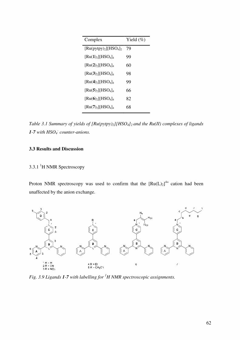
62

Complex Yield (%)

[Ru(pytpy)2][HSO4]2 79

[Ru(1)2][HSO4]4 99

[Ru(2)2][HSO4]4 60

[Ru(3)2][HSO4]4 98

[Ru(4)2][HSO4]4 99

[Ru(5)2][HSO4]4 66

[Ru(6)2][HSO4]4 82

[Ru(7)2][HSO4]4 68

Table 3.1 Summary of yields of [Ru(pytpy)2][HSO4]2 and the Ru(II) complexes of ligands

1-7 with HSO4- counter-anions.

3.3 Results and Discussion

3.3.1 1H NMR Spectroscopy

Proton NMR spectroscopy was used to confirm that the [Ru(L)2]4+

cation had been

unaffected by the anion exchange.

Fig. 3.9 Ligands 1-7 with labelling for 1H NMR spectroscopic assignments.

63

Fig. 3.10 1H NMR spectrum of [Ru(2)2][HSO4]4 in D2O; 500 MHz, 25ºC, TMS.

As previously described (§Ch. 2) for the [Ru(L)2][PF6]4 complexes, the signals were

assigned using the 1D 1H NMR spectrum in conjunction with 2D COSY and NOESY

spectra. The appearance of both one set and the correct number of signals (Fig. 3.10)

confirms that the [Ru(L)2]4+

core of the complex has been unaffected by the anion

exchange. The singlet, for [Ru(2)2][HSO4]4 at δ 6.08 ppm (Fig. 3.10) is assigned to the

Ha proton and is characteristic of this set of complexes. The signal shifts, depending on

the electron-donating or -withdrawing properties of the substituent, between δ 4.78 and

6.14 ppm (L+ = 7 and 3, respectively). When L

+ = 4 (ethyl-substituted) or L

+ = 7 (octyl-

substituted), this signal is coincident with the peak due to residual HOD. This is

confirmed by a cross-peak present in the HMQC spectrum (Fig. 3.11)

NN

N

N

NC

A

B

C

2

3

3

6

5

4

3

a

2

3

D

C3 A

3

B3

C2

A4

D3 D

2 A

6

A5

a

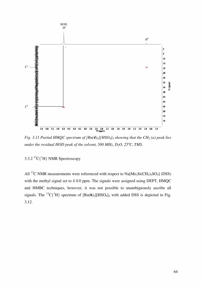
64

Fig. 3.11 Partial HMQC spectrum of [Ru(4)2][HSO4]4 showing that the CH2 (a) peak lies

under the residual HOD peak of the solvent, 500 MHz, D2O, 25ºC, TMS.

3.3.2 13

C1H NMR Spectroscopy

All 13

C NMR measurements were referenced with respect to Na[Me3Si(CH2)3SO3] (DSS)

with the methyl signal set to δ 0.0 ppm. The signals were assigned using DEPT, HMQC

and HMBC techniques, however, it was not possible to unambiguously ascribe all

signals. The 13

C1H spectrum of [Ru(6)2][HSO4]4 with added DSS is depicted in Fig.

3.12.

HOD

Ha

Hb

Ca

Cb

65

Fig. 3.12 13

C1H NMR spectrum of [Ru(6)2][HSO4]4 in D2O; 126 MHz, 25ºC, DSS.

3.3.3 Mass Spectrometry

Electrospray ionisation mass spectrometry (ESI-MS) was used to characterise the

[Ru(pytpy)2][HSO4]2 complex. A peak corresponding to the cation was observed at m/z

361.0, which corresponded to the loss of both anions; [M-2HSO4]2+

.

The [Ru(L)2][HSO4]4 complexes were characterised using MALDI-TOF mass

spectrometry. The fragmentation patterns confirmed successful anion exchange as

fragmentation peaks corresponding to [M-nHSO4]+ (n= 1-3) were observed. Peaks

corresponding to the loss of one substituent were also present for most complexes. The

base peaks, assigned to [Ru(Hpytpy)2]+, [Ru(Hpytpy)(pytpy)]

+ and [Ru(pytpy)2]

+ at m/z

724, 723 and 722, respectively, were also present in the spectra.

3.3.4 Elemental Analysis and Thermogravimetric Analysis

Elemental analysis of [Ru(2)2][HSO4]4 and [Ru(3)2][HSO4]4 pointed to the formation of

hydrates. This was unsurprising given the ability of HSO4- anions to form hydrogen

bonds. It was not possible to obtain elemental analysis of the anhydrous complexes, due

to their hygroscopic nature. Therefore, TGA was used to quantify the theory that the

elemental analyses were consistent with the formation of hydrates. TGA-MS analysis of a

sample of [Ru(3)2][HSO4]4 showed an initial 2.3% weight loss (≤200oC) followed by two

A2/B2

C4

NN

N

N

A

B

C

Hb

HC1

HC2

a

A6

C2

B4

A4

b

A5

C3

A3

c

B3

a

66

further steps of water loss (2.4 and 4.7% weight loss between 200 and 400oC). Sample

decomposition occurred at higher temperatures. The initial degradation steps correspond

to loss of 2H2O, 2H2O and 4H2O, consistent with the elemental analytical data of the

complex: Found: C 42.42, H 3.64, N 9.32; C54H44N10O20RuS4·8H2O requires C 42.49,

H 3.96, N 9.18.

3.3.5 Absorption Spectroscopy

0

25

50

75

220 270 320 370 420 470 520 570 620 670

Wavelength (nm)

ε x

10

-3 (

dm

3 m

ol-1

cm

-1)

1

2

3

4

5

6

7

Ru(pytpy)2

Fig. 3.13 Absorption spectra for [Ru(pytpy)2][HSO4]2 and [Ru(L)2][HSO4]4 (L+ = 1-7),

measured in water at concentrations of 10-6

mol dm-3

.

To be effective as photosensitisers for the POM (§ Introduction), the ruthenium

complexes should ideally absorb over the entire visible spectrum. The broad MLCT

absorptions (390-560 nm for [Ru(pytpy)2][HSO4]2 and 390-580 nm for all other

complexes) cover a large proportion of the visible spectrum.

67

As observed for the [Ru(L)2][PF6]4 complexes (§ Chapter 2) the MLCT band is red-

shifted on alkylation of the pendant pyridyl moiety. The energy of the MLCT band is the

same for [Ru(pytpy)2][PF6]2 and [Ru(pytpy)2][HSO4]2 (λmax = 490 nm) and this is also

true for each [Ru(L)2][HSO4]4 complex, except for [Ru(3)2][HSO4]4 and [Ru(5)2][HSO4]4

(Fig. 3.13), which are slightly red-shifted (518 nm), compared to 513 nm for their PF6-

precursors.

0

10

20

30

40

50

350 400 450 500 550 600 650

Wavelength (nm)

ε x

10

3 (

dm

3 m

ol-1

cm

-1)

[Ru(5)

[Ru(5)

Fig. 3.14 A comparison of the absorption properties of [Ru(5)2][PF6]4 (solid black line)

and [Ru(5)2][HSO4]4 (dashed black line). Concentration = 10-6

mol dm-3

.

The change in anion and solvent, from PF6- in MeCN to HSO4

- in water, affects the

ability of the complexes to absorb light. The molar absorption coefficients for the MLCT

band ranges from 19.6 x 103 (L

+ = 7) dm

3 mol

-1 cm

-1 to 37.8 x 10

3 (L

+ = 1)

for the HSO4

-

salts, compared to 29.7 x 103

(L+ = 3) to 48.7 x 10

3 (L

+ = 7) for the PF6

- salts. In general

the HSO4- water-soluble salts are weaker absorbers than their PF6

- precursors but the ε

values are in the same order of magnitude. However, ε values of 104

mol dm-3

cm-1

means

the complexes are still good absorbers and, therefore, reasonable catalyst candidates35

.

In the UV region of the spectrum the most intense band for the majority of complexes

was around 276 nm. This band arises from a ππ*

transition on the pytpy ligand36

. The

data for all complexes are summarised in Table 3.2.

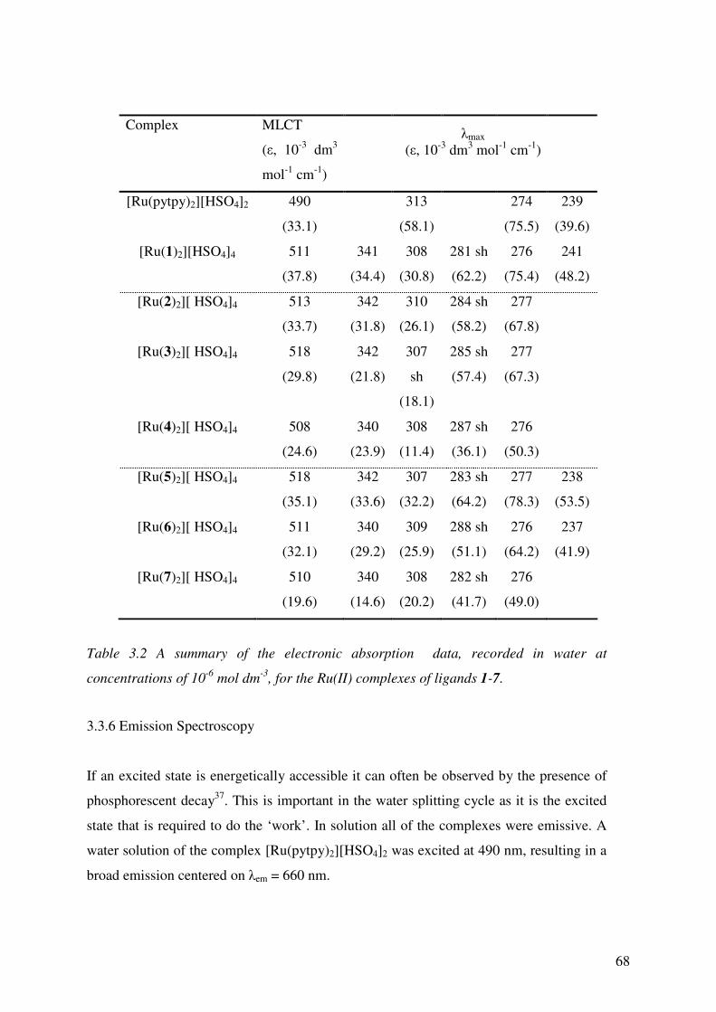
68

Table 3.2 A summary of the electronic absorption data, recorded in water at

concentrations of 10-6

mol dm-3

, for the Ru(II) complexes of ligands 1-7.

3.3.6 Emission Spectroscopy

If an excited state is energetically accessible it can often be observed by the presence of

phosphorescent decay37

. This is important in the water splitting cycle as it is the excited

state that is required to do the ‘work’. In solution all of the complexes were emissive. A

water solution of the complex [Ru(pytpy)2][HSO4]2 was excited at 490 nm, resulting in a

broad emission centered on λem = 660 nm.

Complex MLCT

(ε, 10-3

dm3

mol-1

cm-1

)

[Ru(pytpy)2][HSO4]2 490

(33.1)

313

(58.1)

274

(75.5)

239

(39.6)

[Ru(1)2][HSO4]4 511

(37.8)

341

(34.4)

308

(30.8)

281 sh

(62.2)

276

(75.4)

241

(48.2)

[Ru(2)2][ HSO4]4 513

(33.7)

342

(31.8)

310

(26.1)

284 sh

(58.2)

277

(67.8)

[Ru(3)2][ HSO4]4 518

(29.8)

342

(21.8)

307

sh

(18.1)

285 sh

(57.4)

277

(67.3)

[Ru(4)2][ HSO4]4 508

(24.6)

340

(23.9)

308

(11.4)

287 sh

(36.1)

276

(50.3)

[Ru(5)2][ HSO4]4 518

(35.1)

342

(33.6)

307

(32.2)

283 sh

(64.2)

277

(78.3)

238

(53.5)

[Ru(6)2][ HSO4]4 511

(32.1)

340

(29.2)

309

(25.9)

288 sh

(51.1)

276

(64.2)

237

(41.9)

[Ru(7)2][ HSO4]4 510

(19.6)

340

(14.6)

308

(20.2)

282 sh

(41.7)

276

(49.0)

λmax

(ε, 10-3

dm3 mol

-1 cm

-1)

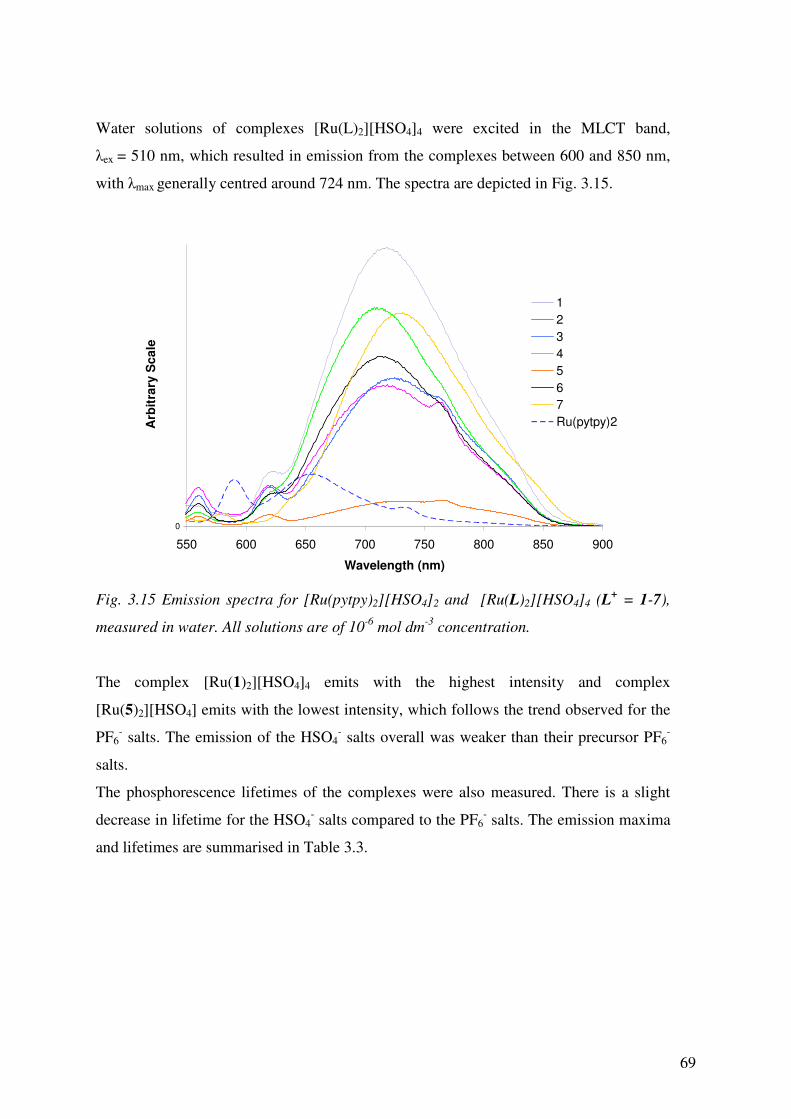
69

Water solutions of complexes [Ru(L)2][HSO4]4 were excited in the MLCT band,

λex = 510 nm, which resulted in emission from the complexes between 600 and 850 nm,

with λmax generally centred around 724 nm. The spectra are depicted in Fig. 3.15.

0

550 600 650 700 750 800 850 900

Wavelength (nm)

Arb

itra

ry S

ca

le

1

2

3

4

5

6

7

Ru(pytpy)2

Fig. 3.15 Emission spectra for [Ru(pytpy)2][HSO4]2 and [Ru(L)2][HSO4]4 (L+ = 1-7),

measured in water. All solutions are of 10-6

mol dm-3

concentration.

The complex [Ru(1)2][HSO4]4 emits with the highest intensity and complex

[Ru(5)2][HSO4] emits with the lowest intensity, which follows the trend observed for the

PF6- salts. The emission of the HSO4

- salts overall was weaker than their precursor PF6

-

salts.

The phosphorescence lifetimes of the complexes were also measured. There is a slight

decrease in lifetime for the HSO4- salts compared to the PF6

- salts. The emission maxima

and lifetimes are summarised in Table 3.3.

70

Table 3.3 A summary of the emission properties of Ru(II) complexes with ligands 1-7,

recorded in water at concentrations of 10-6

mol dm-3

.

Although the lifetimes appear short for phosphorescence it is important to note that the

measurements were carried out at room temperature in aerated solvent and both of these

factors should decrease the lifetime. The measurement was also carried out in water and

the 3O2 present quenches the

3MLCT state, further decreasing the lifetime. The lifetime of

the complex needs to be long enough for the electron transfer to the S2O82-

(reducing it to

SO42-

) and ≥70 ns should be sufficient. The lifetimes are similar to that of an analogous

complex reported by Kaledin et al.35

.

3.3.7 Electrochemistry

Cyclic voltammetry was used to investigate the electrochemical properties of the

complexes selected for testing as WOCs. The complexes selected were

[Ru(pytpy)2][HSO4]2 and [Ru(L)2][HSO4]4 (L+ = 1, 2, 4 and 6).

To be used as a WOC the complex needs to have an oxidation potential above the half

reaction of water oxidation (2H2O → O2 + 4H+ + 4e

-) but within a value that allows for

oxidation. The measurements were carried out in a water solution of the complex using

0.1M NaHSO4 as the electrolyte, with a glassy carbon working electrode, Ag/AgCl

Complex Excitation

Wavelength

(nm)

Emission

Max (nm)

τ (ns)

(+/- 15

ns)

[Ru(pytpy)2][HSO4]2 490 660 73

[Ru(1)2][HSO4]4 510 719 135

[Ru(2)2][HSO4]4 510 722 108

[Ru(3)2][HSO4]4 510 724 103

[Ru(4)2][HSO4]4 510 732 146

[Ru(5)2][HSO4]4 510 734 98

[Ru(6)2][HSO4]4 510 716 137

[Ru(7)2][HSO4]4 510 722 142

71

reference electrode and a Pt wire counter-electrode. The measurements were referenced

to Ag/Ag+. Fig. 3.16 depicts a representative cyclic voltammagram of [Ru(2)2][HSO4]4,

showing only the Ru(II)/Ru(III) oxidation; a meaningful reduction spectrum could not be

obtained.

-3.00E-06

0.00E+00

3.00E-06

0.9 1 1.1 1.2 1.3 1.4

Voltage (V)

Cu

rren

t (A

)

Fig. 3.16 Cyclic Voltammagram for [Ru(2)2][HSO4]4 (H2O, 0.1M NaHSO4, vs. Ag/Ag+).

Only oxidation process shown.

A broad quasi-reversible oxidation wave was observed for all complexes. This was

attributed to the oxidation of RuII to Ru

III. The [Ru(pytpy)2][HSO4]2 complex is more

easily oxidised than the [Ru(L)2][HSO4]4 complexes. The data are summarised in Table

3.4.

Complex Redox potential (V) Eox - Ered (V)

[Ru(pytpy)2][HSO4]2 +1.21 1.25 – 1.16

[Ru(1)2][HSO4]4 +1.24 1.25 – 1.17

[Ru(2)2][HSO4]4 +1.22 1.26 – 1.18

[Ru(4)2][HSO4]4 +1.22 1.26 – 1.17

[Ru(6)2][HSO4]4 +1.22 1.32 - 1.12

Table 3.4 A summary of the redox potentials for Ru(II) complexes with ligands 1-7.

Measurements carried out in water using 0.1M NaHSO4 as the electrolyte and

referenced to Ag/Ag+.

It is reported that [Ru(bpy)3]3+

can act as a water oxidation catalyst18, 19

and so it is

probable that these complexes can also oxidise water. Cyclic voltammetry only gives

information on what is happening at the tip of the electrode and not of the bulk sample.

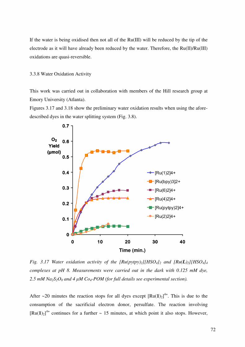
72

If the water is being oxidised then not all of the Ru(III) will be reduced by the tip of the

electrode as it will have already been reduced by the water. Therefore, the Ru(II)/Ru(III)

oxidations are quasi-reversible.

3.3.8 Water Oxidation Activity

This work was carried out in collaboration with members of the Hill research group at

Emory University (Atlanta).

Figures 3.17 and 3.18 show the preliminary water oxidation results when using the afore-

described dyes in the water splitting system (Fig. 3.8).

0000

0.10.10.10.1

0.20.20.20.2

0.30.30.30.3

0.40.40.40.4

0.50.50.50.5

0.60.60.60.6

0.70.70.70.7

0000 10101010 20202020 30303030 40404040

[Ru(1)2]4+

[Ru(bpy)3]2+

[Ru(6)2]4+

[Ru(4)2]4+

[Ru(pytpy)2]4+

[Ru(2)2]4+

OOOO2 2 2 2

Yield Yield Yield Yield

(μmol)(μmol)(μmol)(μmol)

Fig. 3.17 Water oxidation activity of the [Ru(pytpy)2][HSO4]2 and [Ru(L)2][HSO4]4

complexes at pH 8. Measurements were carried out in the dark with 0.125 mM dye,

2.5 mM Na2S2O8 and 4 µM Co4-POM (for full details see experimental section).

After ~20 minutes the reaction stops for all dyes except [Ru(1)2]4+

. This is due to the

consumption of the sacrificial electron donor, persulfate. The reaction involving

[Ru(1)2]4+

continues for a further ~ 15 minutes, at which point it also stops. However,

Time (min.)

73

under these experimental conditions this dye is more effective at oxidising water than the

standard [Ru(bpy)3]2+

dye.

Fig. 3.18 Water oxidation activity of the [Ru(pytpy)2][HSO4]2 and [Ru(L)2][HSO4]4

complexes at pH 9. Measurements were carried out in the dark with 0.125 mM dye,

2.5 mM Na2S2O8 and 4 µM Co4-POM (for full details see experimental section).

On increasing the pH from 8 to 9 the reactions involving all dyes yield a higher amount

of O2. After ~20 minutes the reaction stops for all dyes except [Ru(L)2]4+

(L = 1, 2, 6).

This is due to the consumption of the sacrificial electron acceptor, persulfate. The

reaction involving [Ru(6)2]4+

continues for a further ~ 10 minutes, at which point it also

stops. The reactions involving [Ru(1)2]4+

and [Ru(2)2]4+

continue for 40 minutes. Under

these experimental conditions the [Ru(1)2]4+

dye is again more effective at oxidising

water than the standard [Ru(bpy)3]2+

dye.

The different activities of the complexes are explained as follows:

1. The activity of [Ru(pytpy)2]2+

is expected to be different to that of the other dyes

as it has a +2 charge as opposed to a +4 charge.

0

0.1

0.2

0.3

0.4

0.5

0.6

0.7

0.8

0.9

0 10 20 30 40

[Ru(1)2]4+

[Ru(6)2]4+

[Ru(2)2]4+

[Ru(4)2]4+

[Ru(pytpy)2]2+

[Ru(bpy)3]2+

OOOO2 2 2 2

Yield Yield Yield Yield

(μmol)(μmol)(μmol)(μmol)

Time (min.)

74

2. The initial rates of reaction of the +4 dyes are all the same, which follows the

trend observed in the photophysical and electrochemical properties of the dyes.

3. The change in they dyes’ overall ability to oxidise water can be explained in terms

of their susceptibility to basic attack at the C2 proton (Fig. 3.19).

Fig. 3.19 Proposed mechanism of basic attack at the C2 proton on the terminal pyridyl

rings of the [Ru(L)2]4+

(L = 1, 2, 4, 6) dyes.

Basic attack at C2 destroys the aromaticity of the pyridyl group to form a hydroxopyridyl

species. This species can then be oxidised to form the pyridone, which will behave

differently to the original pyridyl. Confirmation of the different susceptibilities to basic

attack of the complexes can be obtained by looking at the Mulliken charges, using DFT

(Table 3.5).

Complex Stability

(high to low)

Mulliken Charge

on C2

[Ru(pytpy)2]2+

1 0.146

[Ru(2)2]4+

2 0.138

[Ru(4)2]4+

3 0.128

[Ru(6)2]4+

4 0.131

[Ru(1)2]4+

5 0.142

Table 3.5 The relationship between the stability of the dye and the Mulliken Charge on

C2. (DFT carried out using B3LYP/LANL2DZ/6-31G*, see Chapter 2 for details)

As has already been stated, the [Ru(pytpy)2]2+

behaves differently as it has a +2 overall

charge and can therefore be ignored. For complexes [Ru(L)2]4+

(L = 1, 4, 6) the trend in

75

Mulliken charge follows the trend in stability, ie. the more electropositive C2 is, the more

susceptible the complex is to basic attack and, therefore, the less stable that complex is.

The [Ru(2)2]4+

dye behaves differently and this is due to the potential for hydrolysis at the

cyano group, which results in a zwitterion. The charge of the complex subsequently

decreases from +4 to +2 and it would, therefore, be expected to behave in a similar

manner to that of [Ru(pytpy)2]2+

, which is observed experimentally (Fig. 2.19).

3.4 Conclusion

In summary, the [Ru(L)2][HSO4]4 complexes demonstrated very similar photophysical

and photochemical properties to their [Ru(L)2][PF6]4 parent complexes. Selected dyes

showed water oxidation activity when used in conjunction with the Co4-POM of the Hill

group34

. The different catalytic activities of the dyes could be rationalised in terms of the

overall charge of the complex and their susceptibility to basic attack at the C2 position of

the terminal pyridine moiety. Use of the dye [Ru(1)2]4+

resulted in the higest O2 yield and

longest running reaction. Under the experimental conditions used it performed more

effectively than the standard [Ru(bpy)3]2+

dye. Further work in this area should be carried

out into alternative sacrificial electron donors to enable a longer running water oxidation

reaction.

76

3.5 Experimental

General Synthesis of [Ru(L)2][HSO4]4:

The complex [Ru(L)2][PF6]4 was stirred with ten equivalents of [N(tBu)4][HSO4] in a

mixture of 9:1 acetonitrile:dichloromethane for 30 min, during which time a precipitate

formed. The precipitate was filtered over celite and washed with 20 cm3 acetonitrile, then

re-dissolved in deionised water, which was subsequently removed under reduced

pressure, yielding a red powder. The red powder was stirred in 30 cm3 boiling acetonitrile

for 20 min, to remove any remaining [N(tBu)4][PF6], filtered over a sinter and washed

with 20 cm3 EtOH and 20 cm

3 Et2O. The product was isolated as a red powder.

[Ru(pytpy)2][HSO4]2

Yield: 107 mg, 78.7% (starting with 150 mg of [Ru(pytpy)2][HSO4]2)

1H NMR: (500 MHz, D2O, 25ºC, TMS) δ/ppm: 9.30 (s, 4H, B

3),

9.13 (d, J = 5 Hz, 4H, C2), 8.83 (d, J=10 Hz, 4H, C

3), 8.72 (d, J=10 Hz, 4H, A

3),

7.99 (t, J = 20 Hz, 10 Hz, 4H, A4), 7.46 (d, J = 5 Hz, 4H, A

6),

7.22 (t, J = 10, 5 Hz, 4H A5);

13C NMR: (126 MHz, D2O, 25ºC, TMS) δ/ppm: 160.1 (A

2/B

2), 158.8 (A

2/B

2), 156.9 (C

4),

154.9 (A6), 145.2 (C

2), 144.5 (B

4), 141.2 (A

4), 130.5 (A

5), 128.4 (C

3), 127.6 (A

3),

124.7 (B3)

ESI-MS: m/z 361.0 [M-2HSO4]2+

(base peak, calc. 361.1);

Found: C 48.29, H 3.70, N 11.05; C40H30N8O8RuS2·4H2O requires: C 48.63, H 3.88,

N 11.34.

[Ru(1)2][HSO4]4

Yield: 150 mg, 99.1% (starting with 174 mg of [Ru(1)2][HSO4]4)

77

1H NMR: (500 MHz, D2O, 25ºC, TMS) δ/ppm: 9.25 (s, 4H, B

3),

9.21 (d, J = 5.3 Hz, 4H, C2), 8.81 (d, J = 5.3 Hz, 4H, C

3), 8.68 (d, J = 7.7 Hz, A

3),

7.95 (t, J =7.3 Hz, 4H, A4), 7.59 (m, 4H, D

2), 7.56 (m, 6H, D

3+D

4),

7.42 (d, J = 5.2 Hz, 4H, A6), 7.18 (m, 4H, A

5), 5.97 (s, 4H, a).

13C NMR: (126 MHz, D2O, 25ºC, TMS) δ/ppm: 160.0 (A

2/B

2), 158.8 (A

2/B

2),

156.0 (C4), 154.9 (A

6), 148.0 (C

2), 143.7 (B

4), 141.2 (A

4), 135.4 (D

1), 132.9 (D

4),

132.5 (D3), 132.1(D

2), 130.5 (A

5), 129.2 (C

3), 127.6 (A

3), 124.6 (B

3), 67.3 (a).

MALDI-TOF: m/z 1193.1 [M – HSO4]+ (calc. 1195.1).

[Ru(2)2][HSO4]4

Yield: 41.7 mg, 59.6% (starting with 80 mg of [Ru(2)2][HSO4]4)

1H NMR: (500 MHz, D2O, 25ºC, TMS) δ/ppm: 9.28 (s, 4H, B

3),

9.25 (d, J = 5.6 Hz, 4H, C2), 8.87 (d, J = 5.6 Hz, 4H, C

3), 8.70 (d, J = 7.9 Hz, A

3),

7.97 (t, J = 7.6 Hz, 4H, A4), 7.94 (d, J = 8.1 Hz, 4H, D

3), 7.73 (d, J = 8.0 Hz, 4H, D

2),

7.44 (d, J = 5.2 Hz, 4H, A6 ), 7.20 (m, 4H, A

5), 6.09 (s, 4H, a).

13C NMR: (126 MHz, D2O, 25ºC, TMS) δ/ppm: 160.1 (A

2/B

2), 158.8 (A

2/B

2), 155.0 (A

6),

148.4 (C2), 131.2 (A

4), 140.7 (D

1), 136.4 (D

3), 132.4 (D

2), 130.6 (A

5), 129.4 (C

3),

127.7 (A3), 124.7 (B

3), 122.7 (D-C≡N), 115.4 (D

4), 66.5 (a), (C

B4 and C

C4 not resolved).

MALDI-TOF: m/z 839.0 [Ru(2)(Hpytpy)]+ (calc. 839.2), 723.9 [Ru(pytpy)(Hpytpy)]

+

(calc. 723.2). Found: C 46.42, H 3.60, N 10.00; C56H44N10O16RuS4·6H2O requires

C 46.37, H 3.89, N 9.66 (see text).

[Ru(3)2][HSO4]4

Yield: 230 mg, 97.9% (starting with 267 mg of [Ru(3)2][HSO4]4)

1H NMR: (500 MHz, D2O, 25ºC, TMS) δ/ppm: 9.29 (s, 4H, B

3),

9.27 (d, J = 6.4 Hz, 4H, C2), 8.88 (d, J = 5.5 Hz, 4H,

C3), 8.70 (d, J = 7.8 Hz, A

3),

8.39 (d, J =20 8.2 Hz, 4H, D3), 7.97 (t, J = 7.6 Hz, 4H, A

4), 7.80 (d, J =8.2 Hz, 4H, D

2),

7.44 (d, J = 4.7 Hz, 4H, A6), 7.20 (m, 4H, A

5), 6.14 (s, 4H, a).

13C NMR: (126 MHz, D2O, 25ºC, TMS) δ/ppm: 160.0 (A

2/B

2), 158.8 (A

2/B

2), 154.9 (A

6),

78

151.4 (D4), 148.5 (C

2), 143.5 (D

1), 141.2 (A

4), 132.9 (D

2), 130.5 (A

5), 129.5 (C

3),

127.7 (A3), 127.4 (D

3), 124.7 (B

3), 66.1 (a), (B

4 and C

4 not resolved).

MALDI-TOF: 1001.6 [M –3HSO4]+

(calc. 1001.1), 724.0 [Ru(Hpytpy)2]+ (calc. 724.2)

Found: C 42.42, H 3.64, N 9.32; C54H44N10O20RuS4·8H2O requires C 42.49, H 3.96,

N 9.18 (see text).

[Ru(4)2][HSO4]4

Yield: 257 mg, 98.7% (starting with 304 mg of [Ru(4)2][HSO4]4)

1H NMR: (500 MHz, D2O, 25ºC, TMS) δ/ppm: 9.27 (s, 4H, B

3),

9.18 (d, J = 6.3 Hz, 4H, C2), 8.81 (d, J = 6.4 Hz, 4H, C

3), 8.69 (d, J = 7.9 Hz, A

3),

7.96 (t, J = 7.8Hz, 4H, A4), 7.44 (d, J = 5.1 Hz, 4H, A

6), 7.20 (m, 4H, A

5),

4.80 (coincident with solvent, a), 1.75 (t, J = 7.3 Hz, 6H, b).

13C NMR: (126 MHz, D2O, 25ºC, TMS) δ/ppm 160.0 (A

2/B

2), 158.8 (A

2/B

2), 155.5 (C

4),

154.9 (A6), 147.7 (C

2), 143.9 (B

4), 141.1 (A

4), 130.5 (A

5), 129.1 (C

3), 127.6 (A

3),

124.6 (B3), 60.0 (a), 18.4 (b).

MALDI-TOF: m/z 850.4 [Ru(4)(Hpytpy)(HSO4)]+ (calc. 849.2),

821.4 [Ru(Hpytpy)2(HSO4)]+ (calc. 821.1), 751.3 [Ru(4)(Hpytpy)(HSO4)]

+

(calc. 752.2), 723.3 [Ru(pytpy)(Hpytpy)]+ (calc. 723.2).

[Ru(5)2][HSO4]4

Yield: 95.5 mg, 65.9% (starting with 163 mg of [Ru(5)2][HSO4]4)

1H NMR: (500 MHz, D2O, 25ºC, TMS) δ/ppm 9.36 (d, J = 6.5 Hz, 4H, C

2),

9.33 (s, 4H, B3), 8.98 (d, J = 6.6 Hz, 4H, C

3), 8.72 (d, J = 8.1 Hz, A

3),

7.98 (t, J = 7.5 Hz, 4H, A4), 7.45 (d, J = 5.3 Hz, 4H, A

6), 7.21 (m, 4H, A

5),

6.09 (s, 4H, a).

79

13C NMR: (126 MHz, D2O, 25ºC, TMS) δ/ppm 159.9 (A

2/B

2), 158.8 (A

2/B

2), 157.7 (C

4),

154.9 (A6), 148.6 (C

2), 143.1 (B

4), 141.2 (A

4), 130.5 (A

5), 129.6 (C

3), 127.7 (A

3),

124.7 (B3), 116.6 (b), 50.5 (a).

MALDI-TOF m/z 859.8 [Ru(5)(pytpy)(HSO4)]+ (calc. 859.1),

761.6 [Ru(5)(pytpy)]+ (calc. 762.2), 722.3 [Ru(pytpy)2]

+ (calc. 722.2).

[Ru(6)2][HSO4]4

Yield: 148 mg, 81.6% (starting with 210 mg of [Ru(6)2][HSO4]4)

1H NMR: (500 MHz, D2O, 25ºC, TMS) δ/ppm: 9.28 (s, 4H, B

3),

9.16 (d, J = 5.9 Hz, 4H, C2), 8.84 (d, J = 5.8 Hz, 4H, C

3), 8.70 (d, J = 7.9 Hz, 4H, A

3),

7.97 (t, J= 7.6 Hz, 4H, A4), 7.45 (d, J = 5.3 Hz, 4H, A

6), 7.21 (m, 4H, A

5),

6.27 (m, 2H, b), 5.66 (d, J = 10.3 Hz, 2H, c1), 5.63 (d, J = 17.2 Hz, 2H, c2),

5.39 (d, J = 6.1 Hz, 4H, a).

13C NMR: (126 MHz, D2O, 25ºC, TMS) δ/ppm: 160.0 (A

2/B

2), 158.8 (A

2/B

2), 156.0 (C

4),

154.9 (A6), 148.0 (C

2), 143.8 (B

4), 141.2 (A

4), 132.6 (b), 130.5 (A

5), 129.1 (C

3),

127.7 (A3), 126.2 (c), 124.6 (B

3), 66.1 (a).

MALDI-TOF: m/z 803.2 [Ru(6)2]+ (calc. 804.2), 763.2 [Ru(6)(pytpy)]

+ (calc. 763.2),

724.0 [Ru(Hpytpy)2]+ (calc. 724.2).

Found: C 42.84, H 3.65, N 8.99; C46H42N8O16RuS4·5H2O requires C 43.09, H 4.09,

N 8.74 (see text).

[Ru(7)2][HSO4]4

Yield: 35 mg, 68% (starting with 58 mg of [Ru(7)2][HSO4]4)

1H NMR: (500 MHz, D2O, 25ºC, TMS) δ/ppm: 9.29 (s, 4H, B

3),

9.17 (d, J = 6.4 Hz, 4H, C2), 8.83 (d, J = 6.4 Hz, 4H, C

3), 8.71 (d, J = 8.1 Hz, 4H, A

3),

7.98 (t, J = 7.8 Hz, 4H, A4), 7.45 (d, J = 5.4 Hz, 4H, A

6), 7.21 (m, 4H, A

5),

4.78 (t, overlapping solvent, a), 2.13 (m, 4H, b), 1.44 (m, 8H, c+d),

1.34-1.30 (overlapping m, 12H, e+f+g), 0.87 (t, J = 6.8 Hz, 6H, h).

80

13C NMR: (126 MHz, D2O, 25ºC, TMS) δ/ppm: 160.0 (A

2/B

2), 158.8 (A

2/B

2), 155.5 (C

4),

154.8 (A6), 147.9 (C

2), 143.8 (B

4), 141.1 (A

4), 130.4 (A

5), 129.0 (C

3), 127.6 (A

3),

124.6 (B3), 64.7 (a), 33.7 (e/f/g), 33.4 (b), 30.9 (c/d), 30.8 (e/f/g), 28.1 (c/d), 24.7 (e/f/g),

16.2 (h).

MALDI-TOF: m/z 1237.8 [M – HSO4]+ (calc. 1239.3), 949.6 [M – 4HSO4]4

+

(calc. 948.4), 723.3 [Ru(pytpy)(Hpytpy)]3+ (calc. 723.2).

Light-driven Catalytic Experiments

Measurements were carried out by Dr. Yurii Geletii and Hongjin Lv at Emory University

in Atlanta.

The light-driven water oxidation was performed in a cylindrical cuvette (NSG, 32UV10)

with a total volume of ~2.5 ml. The cell was filled with 2.0 ml of reaction solution with

0.125 mM dye, 2.5 mM Na2S2O8, 4 µM Co4P2-POM catalyst (in 80 mM sodium borate

buffer (initial pH 8.0/ 9.0). The reaction cell was sealed with a rubber septum, carefully

deairated and filled with Ar. All procedures were performed with a minimum exposure to

ambient light. The reaction was initiated by turning on the LED-light source (λ = 490 nm;

light intensity 7 mW, beam diameter ~0.4 cm).

A magnetically-coupled stirring system (SYS 114, SPECTROCELL) was used to mix

reaction solutions (4×103 RPM). The O2 concentration in the headspace was quantified

by GC. The solution pH was measured after the reaction.

Analysis of dioxygen in the reaction headspace was performed using a computer

controlled Agilent 6850 model gas chromatograph equipped with a thermal conductivity

detector and a HP-MOLESIEVE capillary GC column (30 m x 0.535 mm x 25.00 µm)

Argon was used as a carrier gas. Typically, the O2 yield was quantified by withdrawing a

gas sample from the headspace without stopping the reaction. Contamination of the head-

space with air was corrected by quantification of N2 present in the head-space (from the

N2 peak in the GC traces).

81

3.6 References

1. G. J. Whitmarch, Encyclopedia of Life Sciences, Macmillan Publ., 2002.

2. J. Barber and M. D. Archer, J. Photochem. Photobiol. A, 2001, 142, 97-106.

3. T. M. I. K.N. Ferreira, K. Maghlaoui, J. Barber, S. Iwata, Science, 2004, 303,

1831-1838.

4. A. Mishra, W. Wernsdorfer, K. A. Abboud and G. Christou, Chem. Commun.,

2005, 54-56.

5. F. M. Ashmawy, C. A. McAuliffe, R. V. Parish and J. Tames, J. Chem. Soc.

Dalton Trans., 1985, 1391-1397.

6. X. Liu and F. Wang, Coord. Chem. Rev., 2012, 256, 1115-1136.

7. H. Yamazaki, A. Shouji, M. Kajita and M. Yagi, Coord. Chem. Rev., 2010, 254,

2483-2491.

8. J. S. V. J. Limburg, L.M. Liable-Sands, A.L. Rheingold, R.H. Crabtree, G.W.

Brudvig, Science, 1999, 283, 1524-1527.

9. G. Sprintschnik, H. W. Sprintschnik, P. P. Kirsch and D. G. Whitten, J. Am.

Chem. Soc., 1976, 98, 2337-2338.

10. R. Zong and R. P. Thummel, J. Am. Chem. Soc., 2005, 127, 12802-12803.

11. J. Hagen, Industrial Catalysis: A Practical Approach, Wiley-VCH, Weinheim,

Germany, 2006.

12. F. Puntoriero, A. Sartorel, M. Orlandi, G. La Ganga, S. Serroni, M. Bonchio, F.

Scandola and S. Campagna, Coord. Chem. Rev., 2011, 255, 2594-2601.

13. B. Limburg, E. Bouwman and S. Bonnet, Coord. Chem. Rev., 2012, 256, 1451-

1467.

14. N. Kaveevivitchai, R. Zong, H.-W. Tseng, R. Chitta and R. P. Thummel, Inorg.

Chem., 2012, 51, 2930-2939.

15. J. J. Concepcion, M.-K. Tsai, J. T. Muckerman and T. J. Meyer, J. Am. Chem.

Soc., 2010, 132, 1545-1557.

16. L. Duan, F. Bozoglian, S. Mandal, B. Stewart, T. Privalov, A. Llobet and L. Sun,

Nature Chem., 2012, 4, 418-423.

17. C. Streb, Dalton Trans., 2012, 41, 1651-1659.

18. Y. V. Geletii, Z. Huang, Y. Hou, D. G. Musaev, T. Lian and C. L. Hill, J. Am.

Chem. Soc., 2009, 131, 7522-7523.

19. Y. V. Geletii, C. Besson, Y. Hou, Q. Yin, D. G. Musaev, D. Quiñonero, R. Cao,

K. I. Hardcastle, A. Proust, P. Kögerler and C. L. Hill, J. Am. Chem. Soc., 2009,

131, 17360-17370.

20. Z. Huang, Z. Luo, Y. V. Geletii, J. W. Vickers, Q. Yin, D. Wu, Y. Hou, Y. Ding,

J. Song, D. G. Musaev, C. L. Hill and T. Lian, J. Am. Chem. Soc., 2011, 133,

2068-2071.

21. Y. V. Geletii, B. Botar, P. Kögerler, D. A. Hillesheim, D. G. Musaev and C. L.

Hill, Angew. Chem. Int. Ed., 2008, 47, 3896-3899.

22. S. Tanaka, M. Annaka and K. Sakai, Chem. Commun., 2012, 48, 1653-1655.

23. D.-L. Long, E. Burkholder and L. Cronin, Chem. Soc. Rev., 2007, 36, 105-121.

24. C. Lydon, C. Busche, H. N. Miras, A. Delf, D.-L. Long, L. Yellowlees and L.

Cronin, Angew. Chem. Int. Ed., 2012, 51, 2115-2118.

25. P. Putaj and F. Lefebvre, Coord. Chem. Rev., 2011, 255, 1642-1685.

26. J. J. Stracke and R. G. Finke, J. Am. Chem. Soc., 2011, 133, 14872-14875.

82

27. J. B. Gerken, J. G. McAlpin, J. Y. C. Chen, M. L. Rigsby, W. H. Casey, R. D.

Britt and S. S. Stahl, J. Am. Chem. Soc., 2011, 133, 14431-14442.

28. M. Natali, S. Berardi, A. Sartorel, M. Bonchio, S. Campagna and F. Scandola,

Chem. Commun., 2012, 48, 8808-8810.

29. K. Heussner, K. Peuntinger, N. Rockstroh, L. C. Nye, I. Ivanović-Burmazović, S.

Rau and C. Streb, Chem. Commun., 2011, 47, 6852-6854.

30. P.-E. Car, M. Guttentag, K. K. Baldridge, R. Alberto and G. R. Patzke, Green

Chem., 2012, 14, 1680-1688.

31. J. J. Walsh, J. Zhu, Q. Zeng, R. J. Forster and T. E. Keyes, Dalton Trans., 2012,

41, 9928-9937.

32. J. J. Walsh, C. T. Mallon, A. M. Bond, T. E. Keyes and R. J. Forster, Chem.

Commun., 2012, 48, 3593-3595.

33. D. Lieb, A. Zahl, E. F. Wilson, C. Streb, L. C. Nye, K. Meyer and I. Ivanović-

Burmazović, Inorg. Chem., 2011, 50, 9053-9058.

34. Q. Yin, J. M. Tan, C. Besson, Y. V. Geletii, D. G. Musaev, A. E. Kuznetsov, Z.

Luo, K. I. Hardcastle and C. L. Hill, Science, 2010, 328, 342-345.

35. A. L. Kaledin, Z. Huang, Q. Yin, E. L. Dunphy, E. C. Constable, C. E.

Housecroft, Y. V. Geletii, T. Lian, C. L. Hill and D. G. Musaev, J. Phys. Chem.

A, 2010, 114, 6284-6297.

36. J. E. Beves, E. L. Dunphy, E. C. Constable, C. E. Housecroft, C. J. Kepert, M.

Neuburger, D. J. Price and S. Schaffner, Dalton Trans., 2008, 386-396.

37. A. Amini, A. Harriman and A. Mayeux, Phys. Chem. Chem. Phys., 2004, 6, 1157-

1164.

83

Chapter 4

Copper(I) Polypyridyl Complexes for Application in DSSCs.

4.1 Introduction

Nearly a decade after the Kyoto treaty1 entered into force there is an increasing usage of

energy sources which offer an alternative to the consumption of fossil fuels. One of these

alternative energy sources is solar energy. There are a number of different types of solar

cell available (§Introduction) and the focus of this project has been on dye-sensitised

solar cells (DSSCs)2.

Dye sensitised solar cells consist of the following components (Fig. 4.1)2-6:

• Counter electrode – This is a transparent conducting oxide and the most

commonly chosen type is fluorine doped tin oxide (FTO).

• Semiconductor – This is the main component of a DSSC. Titanium dioxide

(TiO2) is the most frequently used in DSSCs. It was found that sheets of TiO2

were not efficient enough so nanoparticles are now used7. This results in a larger

surface area, which means that more dye particles can bind per unit area of the

TiO2. There are three polymorphs of TiO2 but anatase is used as it has the largest

energy gap between the valence and the conductance bands (bandgap = 3.2 eV).

• Dye –A dye, which is capable of absorbing visible light and binding to TiO2, is

used as a sensitizer because the band gap of TiO2 is so large it is poor at absorbing

visible light. Research into many organic and inorganic dyes has been carried out

over the years and the most efficient sensitisers to date are based on ruthenium

polypyridyl complexes.

• Redox couple – The most common redox couple is iodide (I-)/triiodide (I3-) but

alternatives include cobalt(II)/cobalt(III), thiocyanate/trithiocyanate and organic

systems such as TEMPO8.

The working principles of a DSSC are depicted in Fig. 4.1.

84

Fig. 4.1 The principles of a dye-sensitised solar cell.

On absorption of light, the dye (S) is promoted to an excited state (S*) as an electron is

transferred from the highest-occupied molecular orbital (HOMO) of the complex, to the

lowest unoccupied molecular orbital (LUMO) (step 1, eqn. 4.1). (This is a simplified

model because there are multiple molecular orbitals close in energy around both the

HOMO and the LUMO.) The electron is then injected into the TiO2 leaving the dye in an

oxidised state (S+) (step 2, Eqn 4.2).

S0 + hυ → S* (Eqn. 4.1)

S* → S+ + e- (Eqn. 4.2)

The counter-electrode donates two electrons to I3-, generating I- (step 3, Eqn. 4.3).

I3- + 2e- (Pt) → 3I- (Eqn. 4.3)

e-

S0/S+

S*

I-/I3-

Load

E

VB

CB

e- e-

e-

FTO TiO2 Dye I3/I3- Counter

electrode

hν

1

2

3

4

85

The I- then reduces the oxidised dye back to its original state (step 4, Eqn. 4.4) and the

whole cycle can start again.

2S+ + 3I- → 2S + I3- (Eqn. 4.4)

Ideally, to be an efficient sensitiser, a dye needs to have the following characteristics2-6, 9:

• It must be able to absorb light over the entire visible spectrum and into the near

infra-red.

• It must have anchoring groups, such as –COOH, -H2PO3, -CN, to enable binding

to the TiO2 nanoparticles.

• In its excited state, the dye must be higher in energy than the conductance band of

the TiO2 so that injection of an electron is faster than excited state decay.

• In its oxidised state, the dye needs to be more positive in energy than the redox

couple, to enable reduction of the dye.

To compare solar cells and determine the efficiency four parameters are used2-6, 9-11.

1. IPCE – Incident monochromatic photon-to-electron conversion, also known as

the external quantum efficiency. The IPCE is defined as the number of electrons,

generated by light, in the external circuit, divided by the number of incident

photons as a function of excitation wavelength.

2. Voc – Open circuit photovoltage. This is determined by the gap between the

electrolyte (ie. redox couple) redox potential and the quasi Fermi level of TiO2

under illumination.

3. Jsc – Short circuit current density. This is the number of electrons being injected

into the TiO2 by the dye and it is limited by the absorption properties of said dye.

For example, a dye with an absorption onset of 800 nm has a theoretical

maximum Jsc of 26 mA cm-2, whereas a dye with an absorption onset of 550 nm

only has a theoretical maximum Jsc of 10 mA cm-2.

4. ff – Fill factor. This is a number between 0 and 1 which expresses the ratio of the

theoretical maximum power to the actual power obtained and is calculated using

Eqn 4.5.

86

ocsc VJ

Pff

×=

max (Eqn. 4.5)

The overall efficiency (η) of a solar cell is calculated as follows (Eqn 4.6):

in

ocsc

P

FFVJ ××=η (Eqn. 4.6)

where Pin is the intensity of the incident light.

Since Graetzel’s first DSSC publication in 19917, ruthenium has been the transition metal

of choice when synthesising dyes for dye-sensitised solar cells and to date the most

efficient DSSCs have been fabricated using ruthenium polypyridyl complexes (Fig 4.2).

“black dye” N719

Fig. 4.2 Two of the best ruthenium polypyridyl complexes to date for application as

sensitisers in DSSCs2, 12.

The dye N719 is often viewed as the research “standard”12 and publications reporting

efficiencies of solar cells using new dyes usually quote the efficiency values with respect

to that of a cell made with N719, fabricated under the same conditions.

However, quoted efficiencies are dependent upon the construction of the cell, electrolyte

etc. and comparisons across a range of measurements carried out in different laboratories

can sometimes be meaningless.

Now, a new area of research is emerging utilising the transition metal, copper. There are

two major advantages of copper over ruthenium. The advantage of copper is its

availability; not only is it much more abundant in the Earth’s crust than ruthenium but it

can also be recovered from scrap metal, it is also easier to extra from its ore than

87

ruthenium. Due to its availaibility, copper is much cheaper than ruthenium. One gram of

ruthenium powder from Sigma Aldrich costs 272 CHF, compared to

one gram of copper powder for 0.20 CHF (prices correct August 2012). The first reported

use of a Cu(I) complex as a photosensitiser was by Sauvage et al in 199413. The complex

consisted of two carboxyphenyl substituted phenanthroline ligands encapsulating a Cu(I)

centre (Fig 4.3).

Fig. 4.3 Tetrasodium bis(2,9-(4-carboxylatophenyl)-1,10-phenanthroline)copper(I)

tetrafluoridoborate. The first Cu(I) complex used as a photosensitiser, reported by

Sauvage et al.13.

In methanol solution the complex showed an MLCT band with λmax = 440 nm (ε = 3000

dm3 mol-1 cm-1) and a shoulder at 560 nm (ε = 1100 dm3 mol-1 cm-1). The dye was

anchored to TiO2 by means of the carboxylate groups and the photocurrent was measured.

The fill factor (ff) was found to be 0.6, the open circuit voltage (Voc) was 0.6 V and the

photocurrent was measured at 0.6 mA cm-2. The fill factor and the open circuit voltage

were reasonable for a DSSC but the photocurrent was very poor.

The next publication describing the use of Cu(I) dyes as photosensitisers was not until

2002 when Hamada et al. reported a homoleptic Cu(I) complex with carboxy

functionalised bipyridine ligands (Fig 4.4)14.

88

Fig. 4.4. Bis(4,4',6,6'-tetramethyl-2,2'-bipyridine-5,5'-dicarboxylic acid) copper(I)

chloride reported by Hamada et al.14.

The complex exhibited an MLCT absorption with λmax = 450 nm

(ε = 6400 dm3 mol-1 cm-1) and as such, was suitable for use as a sensitiser for a DSSC.

The Voc was slightly higher than that of Sauvage’s complex (630 mV) as was the short

circuit current (3.9 mA cm-2). The IPCE was 30% at 460 nm.

Six years later the Constable group reported two complexes (Fig 4.5) which were very

effective photosensitisers, resulting in DSSC devices with efficiencies of 1.9 and 2.3%

(compared to N719 with an efficiency of 9.7%)15.

A B

Fig. 4.5 The two Cu(I) complexes reported by Constable et al. in 200815.

The MLCT band of complex B (λmax = 506 nm) is red-shifted compared to that of

complex A (λmax = 495 nm). Complex B is also more efficient at absorbing light

(ε = 3650 dm3 mol-1 cm-1 compared to ε = 450 dm3 mol-1 cm-1). Therefore, it is

unsurprising that complex B results in a device with a higher efficiency than that of

complex A. (The ff, Jsc, and IPCE values are all higher for the device using complex B

than for the device using complex A.)

89

A further paper detailed similar homoleptic Cu(I) complexes with various substituents

(Fig 4.6)16.

Fig. 4.6 The set of Cu(I) complexes reported by Constable et al. in 200916.

The most efficient device used the copper complex with carboxylic acids in the 5 and 5'

positions of the bipyridine ligands. The efficiency of the device (0.45%), was much

poorer than those previously reported by the same group. However, the efficiency of the

DSSC incorporating N719, prepared in same way, was only 5.0%.

In 2010 Robertson et al. reported the first heteroleptic Cu(I) complex for application in a

DSSC17. To circumvent the challenging synthesis of 6,6'-substituted bipyridines a rigid

POP (POP = bis2-(diphenylphosphanyl)phenylether) ligand was used to sterically

hinder oxidation of the Cu(I) centre. A 4,4'-bis(carboxylic acid) substituted bipyridine

ligand completed the complex (Fig. 4.7).

Fig. 4.7 The first heteroleptic Cu(I) complex tested in a DSSC17.

Assessing the efficacy of this dye is difficult as the efficiency of the device incorporating

N719 was measured as being 3.05%. However, the low efficiency of the copper complex-

containing device (η = 0.053%) is in part due to the irreversibility of the Cu(I)/Cu(II)

oxidation17. If the Cu(II) cannot be reduced by the I-/I3- redox couple, an electrical cycle

90

cannot be established and the device will quickly die. Another deficiency of the dye is

that the MLCT band is only just into the visible region (λmax = 394 nm).

In the same year copper(I) complexes based on N-phenylpyridin-2-methanamine ligands

were reported by Constable et al.(Fig 4.8)18. Although the MLCT bands of these

complexes were in the visible region of the spectrum with λmax = 499-511 nm the

efficiencies of the complexes were very poor; η = 0.23 and 0.006%, compared to N719,

η = 4.60%. The poor efficiencies were explained using low level DFT calculations. These

calculations lead to the conclusion that the LUMO was not on the anchoring moieties of

the complexes, which meant that injection of an electron into TiO2 would be poor.

Fig. 4.8 The two Cu(I) dyes based on N-phenylpyridin-2-methanamine ligands18.

In 2011, a paper reporting DSSC devices using heteroleptic Cu(I) dyes was published19.

In order to make the heteroleptic complexes, Constable et al. exploited the lability of

Cu(I) complexes. By first attaching anchoring ligands (Fig 4.9), such as 6,6'-dimethyl-

[2,2'-bipyridine]-4,4'-carboxylic acid, to TiO2 coated on FTO and then dipping this

electrode into a solution of a homoleptic copper(I) complex, a ligand exchange could be

carried out in situ. This method bypasses the challenge of synthesising and isolating

heteroleptic copper(I) complexes.

Fig. 4.9 Anchoring ligands used by the Constable group19.

91

The homoleptic complexes consisted of a copper(I) ion coordinated to two 6-aryl

substituted bipyridine ligands. Aryl substituents were chosen because thiophene had

previously been used to tune the properties of 2,2'-bipyridine19. The devices using the

phosphonate-substituted anchoring ligand were the most efficient, regardless of the aryl

substituent. The highest efficiency, 1.51%, was obtained after mixing the homoleptic

furan-substituted copper(I) complex with the phosphonate-substituted anchoring ligand

(N719 efficiency = 4.50% measured under the same conditions).

Heteroleptic complexes are desirable for use in DSSCs so that one of the ligands can be

designed with groups that will anchor to the TiO2 and the other ligand can be designed

with groups to optimise the light absorption and redox properties of the complex. In this

chapter one of the homoleptic complexes synthesised is [Cu(dmbpy)2][PF6] (dmbpy =

6,6'-dimethyl-2,2'-bipyridine), chosen due to its structural simplicity20-22. There are

previous reports of the crystal structure of this complex with BF4- counter anion23 and

ClO4- counter anions24 as well as the absorption spectrum of [Cu(dmbpy)2][ClO4] in

ethanol and acetone25 and [Cu(dmbpy)2][PF6] in dichloromethane26. To date there have

been no reports of the full characterisation of [Cu(dmbpy)2][PF6] or its application in

DSSCs. The second homoleptic complex utilises a ligand based on dmbpy which has

extended π-conjugation using triphenylamine groups. Organic DSSCs sensitised with

molecules containing triphenylamine groups have shown promising efficiencies27-29.

In this chapter the same approach to heteroleptic complexes will be used as described in

reference [19].

The ligands 8 and 9 depicted in Fig 4.10, and complexes thereof, are described in this

chapter.

Fig. 4.10 Ligands 8 and 9 with labelling for spectroscopic assignments.

92

4.2 Synthesis of ligand 9 and corresponding Cu(I) complexes

The starting material for 9 was 6,6'-dimethyl-2,2'-bipyridine (8), which was commercially

available. Compound 9 was synthesised by stirring one equivalent of 8 with 2.3

equivalents of 4-(diphenylamino)benzaldehyde in dry DMF for two days in the dark,

using potassium tert-butoxide (KOtBu) as the base (Scheme 4.1). The yield of the

reaction was 55 %.

Scheme 4.1 The synthesis of compound 9.

The synthesis of the copper(I) complexes was carried out by dissolving one equivalent of

[Cu(MeCN)4][PF6] in acetonitrile and stirring (ultrasonicating for 9) it with a chloroform

solution of the relevant ligand for 30 minutes. The solution changed from colourless to

red on addition of the ligand and the product was isolated as a red powder, after

precipitation with diethyl ether (Schemes 4.2 and 4.3).

Scheme 4.2 The synthesis of [Cu(8)2][PF6], yield 77%.

93

Scheme 4.3 The synthesis of [Cu(9)2][PF6], yield 81%.

4.3 Results and Discussion

4.3.2 1H NMR Spectroscopy

[Cu(8)2][PF6] was measured in CD3CN and the spectrum is depicted (Fig 4.11).

Fig. 4.11 1H NMR spectrum of [Cu(8)2][PF6] in CD3CN; 500 MHz, 25ºC, TMS, H2O(*).

*

a

A3 A4

A5

94

The appearance of one set of signals indicates that the complex is homoleptic. The singlet

at δ 2.22 ppm was ascribed to the methyl substituent due to the chemical shift and the

integral.

The triplet at δ 8.02 ppm was ascribed to proton A4 due to the splitting and protons A3

and A5 were assigned by their chemical shift. Proton A

5 is much more shielded than

proton A3 due to the +I effect of the methyl substituent, which means that the signal

ascribed to A5 is further upfield compared to A3.

Fig. 4.12 1H NMR spectrum of 9 in CDCl3; 500 MHz, residual CHCl3 (*), 25ºC, TMS.

The 1H NMR spectrum of 9 (Fig. 4.12) was assigned using both COSY and NOESY

techniques. The starting point for assignment was the triplet at δ 7.81 ppm which, due to

the splitting, had to be ascribed to proton A4. From the COSY spectrum it was then

possible to ascribe the two doublets at δ 8.41 and 7.39 ppm to A3 and A5 by looking for

COSY cross-peaks (Fig. 4.13) from the triplet at δ 7.81 ppm. The specific assignment of

A3 and A5 was done by comparison with a spectrum of 6,6'-dimethyl-2,2'-bipyridine.

*

C3

a + C2

A3 A4

b

B2

A5

C4 + B3

95

Fig. 4.13 Partial COSY spectrum of 9 (500 MHz, CDCl3, 25ºC, TMS) to show cross peaks

between A3, A4 and A5.

Assignment was continued from the broad doublet at δ 7.73 ppm, which had a J coupling

of 16.0 Hz. The large coupling constant indicated that this signal was due to a proton on a

trans-alkene bond. The COSY spectrum (Fig 4.14) enabled location of the other broad

trans-doublet (Fig 4.14) in the overlapping signals at δ 7.15 ppm, highlighted by a red

circle. A NOESY interaction between the peak at δ 7.73 ppm and a doublet at δ 7.15 ppm

(Fig 4.15) meant that the former peak could be ascribed to proton b and the latter peak

ascribed to proton B2. This meant that the broad doublet in the multiplet at δ 7.15 ppm

could be ascribed to proton a. A COSY cross peak between the doublet at δ 7.15 ppm and

the multiplet at δ 7.07 ppm enabled the assignment of the peak at δ 7.07 ppm as B3. A

NOESY correlation is observed between the peak ascribed to B3 and a multiplet at δ 7.15

ppm, which means that the multiplet can be assigned as C2. Protons C

3 and C4 are

subsequently ascribed to the multiplets at δ 7.28 and δ 7.07 ppm, respectively, by

observation of COSY cross peaks with C2.

96

Fig. 4.14 Partial COSY spectrum of 9 (500 MHz, CDCl3, 25ºC, TMS) to show cross peak

between protons a and b. Red circle highlights broad doublet.

Fig. 4.15 Partial NOESY spectrum of 9 (500 MHz, CDCl3, 25ºC, TMS) to show NOE

interaction between the protons ascribed to b and B2.

97

The 1H NMR spectrum of [Cu(9)2][PF6] was measured in CDCl3 and was assigned using

COSY and NOESY techniques (Fig. 4.16).

Fig. 4.16 1H NMR spectrum of [Cu(9)2][PF6] in CDCl3; 500 MHz, residual CHCl3 (*),

25ºC, TMS.

As for compound 9, assignment of the 1H NMR spectrum of [Cu(9)2][PF6] started with

the triplet peak at δ 7.85 ppm, which was ascribed to proton A4. Compared to the ligand

A4 proton, this signal was shifted slightly downfield. COSY correlations identified the

doublets at δ 7.90 and δ 7.74 ppm as A3 and A5. By comparison with the ligand spectrum

the doublet at δ 7.90 ppm could be ascribed to A3 and the doublet at δ 7.74 ppm could be

ascribed to A5.

The signals corresponding to the protons on the A ring of the complex have significantly

different shifts to those of the ligand (Table 4.1), the signal for proton A3 is shifted

upfield and the signal for proton A5 is shifted downfield on complexation. This is due to

the nitrogen atom becoming deshielded by donating electron density to the copper, which

subsequently affects the A ring protons.

N N

N

A

B

C

C

3

5

4

a

b

3

2 9

23

4 N

*

A3 A4 A5

C3

b

C2 + C4

B3 + a B2

98

An NOE interaction between A5 and the broad doublet at δ 7.12 ppm ascribes the broad

doublet to proton b (Fig 4.18). Due to their proximity in space an NOE interaction can be

observed between A5 and b, this interaction is not observed between A5 and a as a is not

conformationally aligned in such a way to allow an NOE interaction to occur. A COSY

correlation between the peak ascribed to b and a broad doublet at δ 6.77 ppm assigns the

broad doublet at δ 6.77 ppm as proton a (Fig 4.17). A NOE interaction between b and the

doublet at δ 6.67 ppm ascribes that doublet to proton B2 (Fig 4.18).

Fig. 4.17 Partial COSY spectrum of [Cu(9)2][PF6] (500 MHz, CDCl3, 25ºC, TMS) to

show cross peak between protons a and b. Red circles highlight broad doublets.

b a

a

b

99

Fig. 4.18 Partial NOESY spectrum of [Cu(9)2][PF6] (500 MHz, CDCl3, 25ºC, TMS) to

show NOE interaction between the protons ascribed to b and A5 (lower line) and b and

B2 (upper line).

From B2 a COSY correlation to the doublet at δ 6.79, which overlaps with the signal for

proton a, enables assignment of said doublet as B3. A weak NOE interaction between B3

and the triplet at δ 7.30 ppm means that the triplet can be ascribed to proton C3. (There is

also a strong NOE interaction between B3 and C

2.) Finally COSY correlations between C3

and the multiplet at δ 7.08 ppm means that the multiplet can be assigned to protons C2

and C4, which is confirmed by the integrals.

On complexation the bipyridine unit of the ligand undergoes a conformational shift from

transoid to cisoid (Fig 4.19), which has a significant effect on the shift of the a, b and B2

peaks in the 1H NMR spectrum (Table 4.1).

b

b

A5

A5

B2

100

Fig 4.19 Conformational changes of ligand 9 on binding to copper.

Compound a b B2

9 7.15 7.74 7.49

[Cu(9)2][PF6] 6.77 7.12 6.67

Table 4.1 Comparison of shifts (δ/ppm) on complexation of compound 9. Spectra

measured in CDCl3 at room temperature.

Compared to the ligand, the signals for protons a and b are shifted upfield. This is

because i) the alkene protons are forced into close proximity with the copper atom and ii)

the effect of the nitrogen atoms on the alkene protons is lessened as the nitrogen atoms

are complexed to copper. The signal for B2 is most affected on complexation of the

ligand and this is due to the close proximity of the protons to the copper ion.

4.3.2 13C NMR Spectroscopy

The 13C1H NMR spectrum of [Cu(8)2][PF6] was measured in CD3CN and assigned

using HMQC and HMBC techniques. The chemical shifts and peak assignments can be

found in the experimental section at the end of this chapter.

The 13C1H NMR spectrum of 9 was measured in CDCl3 and is depicted in Fig 4.20.

101

Fig. 4.20 13C1H NMR spectrum of 9 in CDCl3; 126 MHz, 25ºC, TMS.

The peaks arising from 13C-H carbons were assigned using the HMQC spectrum. The

cross-peaks involving the alkene protons and their respective carbon signals were very

distinct (Fig 4.21). The quaternary carbon signals were assigned using the HMBC

spectrum. Proton C3 had an HMBC interaction with a signal at δ 147.5 ppm, which was

assigned to C1. Proton B2 had a HMBC interaction with a signal at δ 148.5 ppm, which

was assigned to B4. Proton B

3 had a HMBC interaction with a signal at δ 130.8 ppm,

which was assigned to B1. Proton A4 had HMBC interactions with signals at δ 156.1 and

δ 155.3 ppm, which were assigned to the A ring (Fig 4.22). Proton b had an HMBC

interaction with the signal at δ 155.3 ppm, which was assigned to A6 (Fig 4.22). By

deduction, the signal at δ 156.1 ppm was then assigned to A2.

A2 A6 B4

C1

A4 B1 b

B3+C4

A5 A3

B2

a

C3 C2

102

Fig 4.21 Partial HMQC spectrum of compound 9, measured in CDCl3 at 25ºC.

Fig 4.22 HMBC spectrum of compound 9, measured in CDCl3 at 25ºC, depicting the

interactions between H(A4) and C(A2), C(A6) and H(b) and C(A6) specifically.

a

b

b a

A3 A4 b

A2

A6

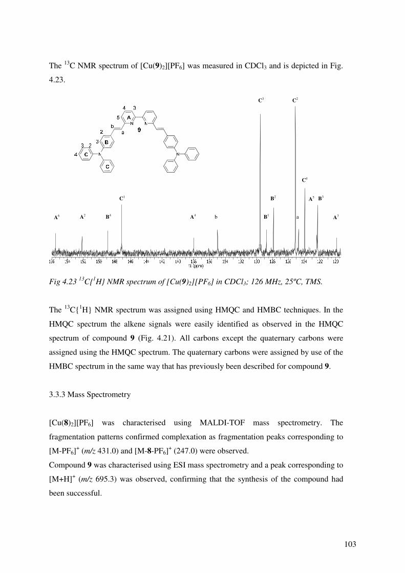
103

The 13C NMR spectrum of [Cu(9)2][PF6] was measured in CDCl3 and is depicted in Fig.

4.23.

Fig 4.23 13C1H NMR spectrum of [Cu(9)2][PF6] in CDCl3; 126 MHz, 25ºC, TMS.

The 13C1H NMR spectrum was assigned using HMQC and HMBC techniques. In the

HMQC spectrum the alkene signals were easily identified as observed in the HMQC

spectrum of compound 9 (Fig. 4.21). All carbons except the quaternary carbons were

assigned using the HMQC spectrum. The quaternary carbons were assigned by use of the

HMBC spectrum in the same way that has previously been described for compound 9.

3.3.3 Mass Spectrometry

[Cu(8)2][PF6] was characterised using MALDI-TOF mass spectrometry. The

fragmentation patterns confirmed complexation as fragmentation peaks corresponding to

[M-PF6]+ (m/z 431.0) and [M-8-PF6]

+ (247.0) were observed.

Compound 9 was characterised using ESI mass spectrometry and a peak corresponding to

[M+H]+ (m/z 695.3) was observed, confirming that the synthesis of the compound had

been successful.

A5

A6 A2 B4

C1

A4 b

C3

B1

B2

C2

a

C4

B3

A3

104

[Cu(9)2][PF6] was also characterised using ESI mass spectrometry. Successful

complexation was confirmed by the observation of a peak corresponding to [M-PF6]+

(m/z =1453.7) in the spectrum. The base peak, assigned to [9+H]+ (m/z 695.3), was also

present in the spectrum.

4.3.4 Absorption Spectroscopy

As discussed in the introduction to this chapter, to be truly efficient as photosensitisers

for DSSCs the copper complexes should ideally absorb over the entire visible spectrum.

There are currently many examples of ruthenium complexes which have this property,

the most famous being “the black dye”30, but no copper complexes yet meet this criterion.

Whilst copper complexes are not at this stage of development, they do give rise to an

MLCT band in the red-orange region of the spectrum, thus absorbing some visible light.

UV-vis spectroscopy was used to ascertain how much light from the visible spectrum was

absorbed by the compounds described in this chapter.

0

5

10

15

20

25

30

220 270 320 370 420 470 520 570

Wavelength (nm)

ε x

10

-3 (

dm

3 m

ol-1

cm

-1)

[Cu(8)2][PF6]

8

Fig. 4.24 Absorption spectra for 8 (red line) and [Cu(8)2][PF6](black line) measured in

MeCN with a concentration of 10-5 mol dm-3.

Compared to the ligand (8), the complex is much more strongly absorbing (Fig. 4.24). A

new band with λmax = 452 nm is observed for the complex, which gives rise to its red

105

colour and means that the complex absorbs visible light. This band is due to an MLCT

transition; promotion of an electron from an occupied copper d-orbital to an empty ligand

π* orbital. The UV region of the spectrum is dominated by ligand-based π→π*

transitions. The data are summarised in Table 4.2.

Table 4.2 A summary of the absorbance data, recorded in acetonitrile, for 8 and

[Cu(8)2][PF6] with concentrations of 10-5 mol dm-3.

0

50

100

150

200

250

250 300 350 400 450 500 550 600

Wavelength (nm)

ε x

10

-3 (

dm

3 m

ol-1

cm

-1)

9

[Cu(9)2][PF6]

Fig. 4.25 Absorption spectra of 9 (green line) and [Cu(9)2][PF6] (blue line) measured in

CH2Cl2 with concentrations of 10-6 mol dm-3.

The absorptions of compound 9 and its copper(I) complex (Fig. 4.25) are much more

intense than those of the [Cu(8)2][PF6] complex. This is due to the extended π-system of

ligand 9, compared to ligand 8. The spectrum of 9 contains two peaks with λmax = 296

and 389 nm. The latter absorption gives rise to the yellow-orange colour of the compound.

Compound MLCT

(ε, 103 dm3

mol-1 cm-1)

8 300

(1.07)

289

(1.70)

245

(1.05)

239

(1.13)

[Cu(8)2][PF6] 457

(3.47)

311 sh

(18.68)

302

(27.19)

266

(18.66)

246

(20.3)

241 sh

(18.90)

λmax (ε, 103 dm3 mol-1 cm-1)

106

In the case of the complex [Cu(9)2][PF6] these peaks are slightly red-shifted to 299 and

400 nm. The peak with λmax = 400 nm tails further into the visible region, giving rise to

the orange colour of the complex. Contrary to the case of [Cu(8)2][PF6], no MLCT peak

is observed in the UV-vis spectrum of [Cu(9)2][PF6] and this is explored later using DFT

and TD-DFT (§ Chapter 5). The data for both compounds are summarised in Table 4.3.

Compound

9 296 (53.6) 389 (97.3)

[Cu(9)2][PF6] 299 (185.4) 400 (235.5)

Table 4.3 A summary of the absorption data, recorded in dichloromethane, for 9 and

[Cu(9)2][PF6]

4.3.5 Excitation and Emission Spectroscopy

In the cycle of a DSSC it is the excited state of the copper complex that does the ‘work’,

which in this case is the donation of an electron to the titanium dioxide. If an excited state

is energetically accessible it can be observed by the presence of luminescent decay,

provided that the lifetime is sufficiently long and the non-radiative processes are not too

efficient. Emission spectroscopy was used to identify luminescent decay and, in the case

of 9 and [Cu(9)2][PF6], excitation spectroscopy was used to confirm the origin of the

emission.

The excitation and emission spectra of [Cu(8)2][PF6] were measured in acetonitrile and

the spectra are depicted in Fig. 4.26.

λmax (ε, 103 dm3 mol-1 cm-1)

107

0

300 400 500 600 700 800

Wavelength (nm)

Arb

itra

ry S

cale

ex 300

ex 454

Fig. 4.26 Emission spectra of [Cu(8)2][PF6] measured in acetonitrile after exciting into a

ligand-based absorption at 300 nm and the MLCT band at 454 nm.

Excitation into the ligand-based absorption band at 300 nm gives rise to a ligand-based

emission in the UV region of the spectrum with λem = 351 nm, which tails into the visible

region of the spectrum. Excitation into the MLCT band results in two emissions. The first

in the blue-green region of the spectrum, with λem = 525 nm and the second in the orange-

red region, with λem = 690 nm, which also tails into the red region.

The lifetime of the emission with λem = 525 nm was 4 ns and the lifetime of the emission

with λem = 690 nm was 2 ns. For application in DSSCs the lifetime of the complex needs

to be longer than the timescale of electron injection from the complex in its excited state

into TiO2. Electron injection happens on the picosecond timescale2 and as such this

complex fulfils said criterion. An attempt was made to measure the quantum yield of the

complex using the Quantaurus instrument but the quantum yield was below the detectable

limit of the machine (< 0.1%).

108

0

250 300 350 400 450 500 550 600 650

Wavelength (nm)

Arb

itra

ry S

ca

le

ex 299

ex 391

em 473

Fig. 4.27 Emission and excitation spectra of 9 measured in dichloromethane depicting

emission spectra from excitation into the absorption bands at 299 and 391 nm and an

excitation spectrum recorded after scanning the excitation holding the emission at

473 nm.

Excitation into the absorption bands at 291 and 391 nm of compound 9, gave rise to the

same emission spectrum, which has λem = 473 nm (Fig. 4.27). By holding the emission at

473 nm and scanning the excitation wavelengths, the excitation spectrum of the complex

is obtained, which consists of two peaks with λex = 291 and 391 nm. This confirms the

origin of the emission with λem = 473 nm.

109

0

200 250 300 350 400 450 500 550 600

Wavelength (nm)

Arb

itra

ry S

cale

ex 300

em 342

em 475

Fig. 4.28 Emission and excitation spectra of [Cu(9)2][PF6] measured in

dichloromethane depicting an emission spectrum (-) from excitation into the absorption

band at 300 nm and an excitation spectra after scanning the excitation holding the

emission at 342 (-·-) and then 475(- -) nm.

Excitation into the absorption band at 300 nm of complex [Cu(9)2][PF6] (Fig. 4.28) gives

rise to two emissions. One emission is very weak and has λem = 342 nm, the other

emission is stronger and has λem = 475 nm. The latter emission is the same as that

observed for the ligand (compound 9). From the excitation spectrum it can be determined

that the emission also has the same origin as that of the ligand, namely the absorption

around 391 nm. This is unsurprising given the similarity of the absorption spectra of the

ligand and its corresponding copper complex. Measuring the excitation spectrum whilst

holding the emission at 342 nm gives rise to a peak with λex = 257 nm. The emission at

342 nm is, therefore, ligand-based.

The data for ligand 9 and its copper complex are summarised in Table 4.4.

Compound

λex λem λem λex λem

9 291 473 391 473 [Cu(9)2][PF6] 300 342 475

Table 4.4 A summary of the emission data, recorded in dichloromethane, for 9 and

[Cu(9)2][PF6]

110

The lifetime of the [Cu(9)2][PF6] complex was 2 ns, which is longer than the rate of

electron injection. The quantum yield of the complex was reasonable; 37 % in aerated

dichloromethane solution at room temperature.

4.3.6 Electrochemistry

A desirable property of a dye for DSSC application is that it is able to donate an electron

to TiO2. A further desirable property is that the oxidised dye can be reduced back to the

ground state by the I-/I3- redox couple. The oxidation potential of a dye can be explored

using cyclic voltammetry.

All measurements were carried out using a solution of the complex in an organic solvent

(see figure captions for details), using 0.1M TBAPF6 as the electrolyte, a glassy carbon

working electrode, Pt wire as the counter-electrode and silver wire as a pseudo-reference

electrode, measurements were referenced to Fc/Fc+.

-8.0

-6.0

-4.0

-2.0

0.0

2.0

-2.5 -2 -1.5 -1 -0.5 0 0.5 1 1.5

Potential vs Fc/Fc+

(V)

Cu

rre

nt

(µA

)

Fig. 4.29 Cyclic Voltammagram for [Cu(8)2][PF6] (MeCN, 0.1M TBAPF6, internal

reference; ferrocene), oxidative (black) and reductive (blue) scans shown.

In the oxidative cycle of [Cu(8)2][PF6] (Fig. 4.29), a reversible, one-electron oxidation

wave is observed at E1/2 = + 0.17 V. This is attributed to a Cu(I)/Cu(II) oxidation. The

low oxidation potential and reversibility mean that this dye is a potential candidate for

application in DSSCs.

111

Two reductions are observed in the reductive cycle (Fig. 4.29); a small peak at -1.37 V

and a large peak at -1.79 V. The peak at -1.13 V could either correspond to the reduction

at -1.37 V, rendering said peak quasi-reversible, or it could be due to deposition of by-

products from decomposition of the complex.

-1.5E-06

-5.0E-07

5.0E-07

1.5E-06

2.5E-06

0 0.2 0.4 0.6 0.8 1

Potential vs Fc/Fc+ (V)

Cu

rren

t (A

)

Fig. 4.30 Cyclic Voltammagram for 9 measured (dichloromethane, 0.1M TBAPF6,

internal reference; ferrocene).

Three oxidation waves are observed in the cyclic voltammagram of 9 (Fig 4.30). The first,

with E1/2 = 0.43 V, and second, with E1/2 = 0.47 V, are largely reversible. The third, at

0.66 V, is very broad and could be due to a slow electron transfer or two overlapping one

electron processes. The extensive overlapping means that it is difficult to ascertain

reversibility. It is postulated that the oxidation of the compound leads to the sequential

formation of radical cations centered on the triphenylamine groups. In order to obtain

more information spectroelectrochemistry was employed (Fig. 4.31).

112

0

0.05

0.1

0.15

0.2

0.25

250 300 350 400 450 500 550 600

Wavelength (nm)

Ab

so

rban

ce

no voltage

0 V

0.1 V

0.2 V

0.3 V

0.4 V

0.5 V

0.6 V

0.7 V

0.8 V

0.9 V

1.0 V

1.1 V

1.2 V

1.3 V

1.4 V

1.5 V

Fig. 4.31. Spectroelectrochemistry of ligand 9, measured in dichloromethane.

Using spectroelectrochemistry it is possible to observe changes in the UV-vis spectrum of

the compound as a result of changing the voltage. The peak at λmax = 302 nm is due to the

bipyridine unit31 and is only slightly affected by increasing the voltage. The peak at

λmax = 399 nm is greatly affected on increasing the voltage, which indicates that the

triphenylamine group is being oxidised. The growth of the peak with λmax = 505 nm is

indicative of the formation of a radical cation as removal of an electron from the HOMO

raises the level of the SHOMO (second highest occupied molecular orbital), decreasing

the HOMO-LUMO gap and, therefore, giving rise to a peak at a longer wavelength than

the original32. This also puts forward the postulation that although many processes are

observed in the cyclic voltammagram, they are similar processes occurring over the

triphenylamine moieties at opposite sides of the molecule as there is only one overall

change in the UV-vis spectrum on oxidation, confirmed by the isosbestic point in the

spectroelectrochemistry.

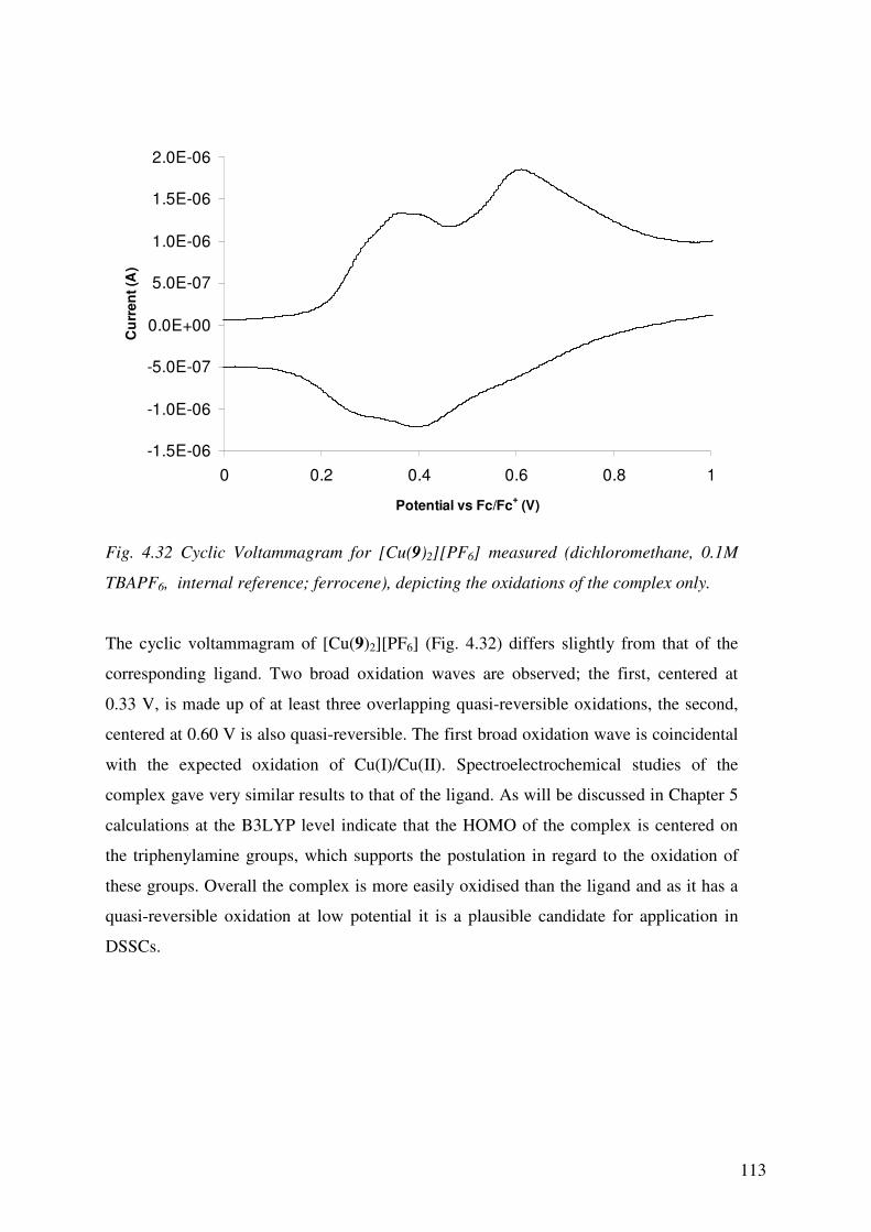
113

-1.5E-06

-1.0E-06

-5.0E-07

0.0E+00

5.0E-07

1.0E-06

1.5E-06

2.0E-06

0 0.2 0.4 0.6 0.8 1

Potential vs Fc/Fc+ (V)

Cu

rre

nt

(A)

Fig. 4.32 Cyclic Voltammagram for [Cu(9)2][PF6] measured (dichloromethane, 0.1M

TBAPF6, internal reference; ferrocene), depicting the oxidations of the complex only.

The cyclic voltammagram of [Cu(9)2][PF6] (Fig. 4.32) differs slightly from that of the

corresponding ligand. Two broad oxidation waves are observed; the first, centered at

0.33 V, is made up of at least three overlapping quasi-reversible oxidations, the second,

centered at 0.60 V is also quasi-reversible. The first broad oxidation wave is coincidental

with the expected oxidation of Cu(I)/Cu(II). Spectroelectrochemical studies of the

complex gave very similar results to that of the ligand. As will be discussed in Chapter 5

calculations at the B3LYP level indicate that the HOMO of the complex is centered on

the triphenylamine groups, which supports the postulation in regard to the oxidation of

these groups. Overall the complex is more easily oxidised than the ligand and as it has a

quasi-reversible oxidation at low potential it is a plausible candidate for application in

DSSCs.

114

4.3.7 Crystal Structures

Red blocks of [Cu(8)2][PF6] were grown by diffusing diethyl ether into an acetonitrile

solution of the complex. The structure solved in the monoclinic P21/c space group with a

very good R factor of 2.93 %. The asymmetric unit contains one cation and one PF6-

anion. The structure of the cation is depicted in Fig. 4.33.

Fig. 4.33 Structure of [Cu(8)2][PF6] with ellipsoids plotted at 50% probability and the

hydrogens removed for clarity. Selected bond parameters: Cu1-N1 =2.0249(9),

Cu1-N2 = 2.0471(9), Cu1-N3 = 2.0446(9), Cu1-N4 = 2.0335(9) Å;

N1-Cu1-N2 = 81.13(4), N1-Cu1-N3 = 127.51(4), N3-Cu1-N4 = 81.59(4),

N2-Cu1-N4 = 132.08(4)°.

The structures of [Cu(8)2][BF4]23 and [Cu(8)2][ClO4]

24 have previously been reported. By

comparison, the Cu-N1 and Cu-N4 bond lengths in the structure of [Cu(8)2][PF6] are

slightly shorter and the Cu-N2 and Cu-N3 bond lengths are slightly longer than those of

previously reported structures (Table 4.5). The N1-Cu-N2 and N3-Cu-N4 bond angles are

smaller than those reported for [Cu(8)2][BF4] and the same as those reported for

[Cu(8)2][ClO4] (Table 4.5). The N1-Cu-N3 bond angle is smaller and the N2-Cu-N4 bond

angle is larger than those reported for both [Cu(8)2][BF4] and [Cu(8)2][ClO4] (Table 4.5)

N1 N2

N3

N4

Cu1

115

Bond (Å)/ Angle (°)

[Cu(8)2][BF4] [Cu(8)2][ClO4] [Cu(8)2][PF6]

Cu- N1 2.052(1) 2.047(2) 2.0249(9) Cu-N2 2.018(1) 2.029(2) 2.0471(9) Cu-N3 2.024(1) 2.021(2) 2.0446(9) Cu-N4 2.040(1) 2.045(2) 2.0335(9) N1-Cu-N2 81.66(6) 81.13(9) 81.13(4) N3-Cu-N4 82.22(6) 81.72(10) 81.59(4) N1-Cu-N3 128.46(4) 130.42(9) 127.51(4) N2-Cu-N4 130.33(7) 128.48(9) 132.08(4)

Table 4.5 Comparison of selected bond parameters for [Cu(8)2][BF4], [Cu(8)2][ClO4]

and [Cu(8)2][PF6].

The angle between the two bipyridine planes is 76.37°, which is considerably smaller

than that observed in the structures of [Cu(8)2][BF4] (80.9°) and [Cu(8)2][ClO4] (80.7°).

As in the case of [Cu(8)2][BF4] and [Cu(8)2][ClO4], the bipyridine ligands are not planar

and twists of 10.56° around the N3-N4 bipyridine and 0.61° around the N1-N2 bipyridine

C-C bonds are present in the structure.

The [Cu(8)2]+ cations pack in chains (Fig. 4.34). There is one crystallographically

independent CH-π interaction between H141 and the py ring containing N2 (x, y, -1+z)

which leads to propagation of chains that follow the crystallographic c axis (Fig 4.35).

There are also extensive CH….F interactions throughout the lattice.

Fig. 4.34 Packing of the [Cu(8)2]+ cations viewed along the (left) a axis and (right) b axis.

116

Fig. 4.35 Face to edge interaction between H141 and the ring including N2 (H141-

centroid distance = 2.587 Å).

Yellow plates of 9 were grown by slowly diffusing hexanes into a dichloromethane

solution of the compound. The structure solved in the orthorhombic Pbca space group

with an R factor of 3.84 %. The asymmetric unit contains half a molecule. The second

half of the molecule is generated by symmetry and is related to the first half by an

inversion centre.

The structure of the molecule is depicted in Fig. 4.36 and selected bond lengths and

angles are listed in the caption.

117

Fig. 4.36 Structure of 9 with ellipsoids plotted at 50% probability and hydrogens omitted

for clarity. Selected bond parameters: N1-C5 = 1.352(2), C5-C6 = 1.467(2),

C6-C7 = 1.337(2), C7-C8 = 1.461(2), C11-N2 = 1.425(2), N2-C14 = 1.418(2),

N2-C20 = 1.417(2) Å; N1-C5-C6 = 117.6(1), C5-C6-C7 = 123.7(1),

C6-C7-C8 = 127.2(1), C11-N2-C14 = 119.3(1), C11-N2-C14 = 119.3(1),

C14-N2-C20 = 120.3(1)°.

As expected the bipyridine unit is in the trans-conformation. This is to minimise electron

repulsion between the two nitrogen lone pairs. Due to half of the molecule being

generated by symmetry the bipyridine unit is planar. The bond lengths around the

bipyridine ring and triphenylamine unit are unexceptional. The C5-C6 and C7-C8 bond

lengths are consistent with single bonds. In comparison, the C6-C7 bond is contracted

and has a smaller bond length, which is consistent with a double bond. The C8-C13 ring

is twisted slightly, relative to the bipyridine, and the angle between the planes is 30.11°

(Plane 1 = ring containing N1, plane 2 = ring containing C8).

The molecules pack with intermeshing triphenylamine moieties (Figs. 4.37 and 4.38).

There are no interactions between the bipyridine moieties.

N1 N2

C5 C6

C7 C8

C11

C20

C14

118

Fig. 4.37 Packing of the molecules, (left) atoms coloured by element, (right) red and blue

colours highlight the intermeshing of the triphenylamine units. Both viewed along the a

axis.

Fig. 4.38 Packing of the molecules, (top) atoms coloured by element, (bottom) red and

blue colours highlight the intermeshing of the triphenylamine units. Both viewed along

the b axis.

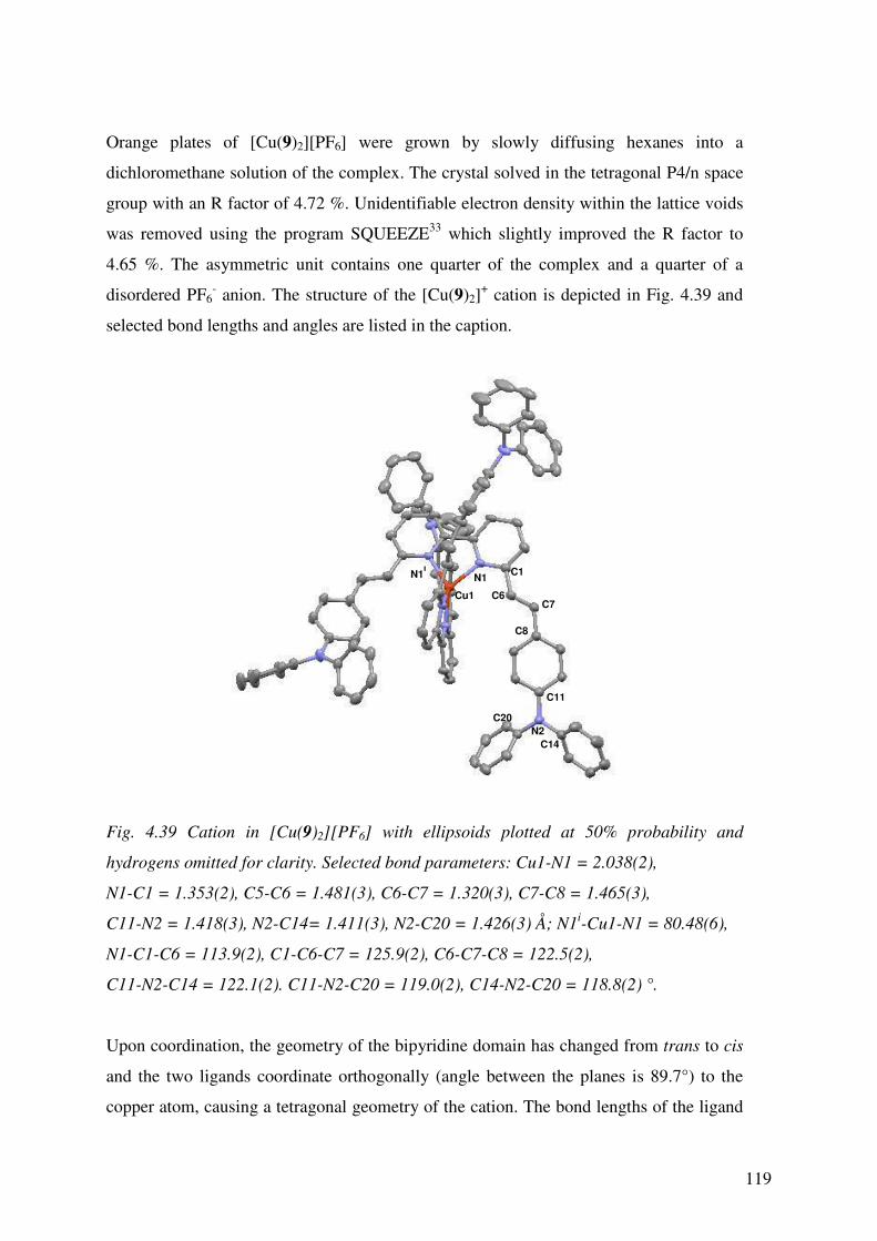
119

Orange plates of [Cu(9)2][PF6] were grown by slowly diffusing hexanes into a

dichloromethane solution of the complex. The crystal solved in the tetragonal P4/n space

group with an R factor of 4.72 %. Unidentifiable electron density within the lattice voids

was removed using the program SQUEEZE33 which slightly improved the R factor to

4.65 %. The asymmetric unit contains one quarter of the complex and a quarter of a

disordered PF6- anion. The structure of the [Cu(9)2]

+ cation is depicted in Fig. 4.39 and

selected bond lengths and angles are listed in the caption.

Fig. 4.39 Cation in [Cu(9)2][PF6] with ellipsoids plotted at 50% probability and

hydrogens omitted for clarity. Selected bond parameters: Cu1-N1 = 2.038(2),

N1-C1 = 1.353(2), C5-C6 = 1.481(3), C6-C7 = 1.320(3), C7-C8 = 1.465(3),

C11-N2 = 1.418(3), N2-C14= 1.411(3), N2-C20 = 1.426(3) Å; N1i-Cu1-N1 = 80.48(6),

N1-C1-C6 = 113.9(2), C1-C6-C7 = 125.9(2), C6-C7-C8 = 122.5(2),

C11-N2-C14 = 122.1(2). C11-N2-C20 = 119.0(2), C14-N2-C20 = 118.8(2) °.

Upon coordination, the geometry of the bipyridine domain has changed from trans to cis

and the two ligands coordinate orthogonally (angle between the planes is 89.7°) to the

copper atom, causing a tetragonal geometry of the cation. The bond lengths of the ligand

N1

Cu1 C6

C1

C7

C8

C11

N2

C20

C14

N1i

120

are virtually unchanged on coordination. Of note are the C1-C6 and N2-C20 bonds,

which are slightly elongated upon complexation. As in the case of the ligand the short

C6-C7 bond lengths are confirmation of a double bond.

The ligands wrap tightly around the Cu+ ion (Fig 4.40) which probably causes the twist in

the bipyridine (angle between pyridine planes is 16.6º).

Fig. 4.40 Space-filling diagram of the [Cu(9)2]+ cation in [Cu(9)2][PF6] with the two

ligands shown in red and blue. The complexes pack with intermeshing triphenylamine groups (Fig 4.41). Similarly to the

packing of compound 9, there are no interactions between the bipyridine groups. The

numerous CH….F interactions throughout the lattice play an important role in the crystal

packing.

Fig. 4.41 Packing of the cations with red and blue colours highlighting the intermeshing

of the triphenylamine units, (right) viewed along the a axis, (bottom) viewed along the b

axis.

121

4.3.8 DSSCs Incorporating the Cu(I) Complexes

The following discussion is based on data obtained by Liselotte Siegfried and Dr. Biljana

Bozic-Weber in the in-house solar cell laboratory.

The lability of Cu(I) has been exploited to form heteroleptic complexes bound to titanium

dioxide, starting from a homoleptic complex in the following step-wise manner:

First, the anodes for the solar cells (see experimental section) were dipped into DMSO

solutions of ligands 10, 11, 12 or 13 (Fig. 4.42). After washing and drying, the electrodes

were immersed in EtOH solutions of [Cu(8)2][PF6] or CH2Cl2 solutions of [Cu(9)2][PF6]

for 64 hours. During this period, the TiO2 changed from colourless to orange. When the

slides were washed with EtOH, the orange colour was retained, indicating that ligand

exchange at copper(I) had occurred with formation of a surface-bound heteroleptic

complex. It is unlikely that the bound species is the homoleptic complex [Cu(L)2]+ (L = 8,

9) since ligands 8 and 9 have no substituents capable of binding the complex to the

surface.

The anchoring ligands that were used are depicted in Fig 4.42.

Fig. 4.42 Structures of the anchoring ligands, 10-13. The anchoring groups are the

carboxylic or phosphonic acids or their conjugate bases.

The cells were measured two days after sealing and the efficiencies are given in Table 4.6.

Cells made using complex [Cu(9)2][PF6] were generally more efficient than those made

with [Cu(8)2][PF6]. The greater efficiency is attributed in part to the greater light-

harvesting ability of [Cu(9)2][PF6] due to the extended π-conjugation of the ligand. It is

also thought that the bulky triphenylamine groups may help to minimise back migration

of an electron from the semiconductor to the dye (§ Chapter 5).

For both starting complexes, ligand exchange with 11 or 12 resulted in DSSCs with the

highest efficiency and this is consistent with previously reported DSSCs made in the

122

Constable group19. Combination with ligand 13 resulted in DSSCs with the poorest

overall efficiencies and this may be due to steric crowding at the copper(I) centre,

particularly in the case of [Cu(9)(13)][PF6].

[Cu(L)2]+ L' Jsc / A cm-2 Voc / mV ff η / %

[Cu(8)2]+ 10 0.003 518 0.58 1.03

[Cu(8)2]+ 11 0.004 618 0.46 1.18

[Cu(8)2]+ 12 0.006 563 0.45 1.63

[Cu(8)2]+ 13 0.001 536 0.64 0.49

[Cu(9)2]+ 10 0.001 482 0.65 0.47

[Cu(9)2]+ 11 0.005 609 0.60 1.95

[Cu(9)2]+ 12 0.005 555 0.60 1.70

[Cu(9)2]+ 13 0.001 555 0.63 0.51

N719 0.018 718 0.58 7.29

Table 4.6 DSSC efficiency data two days after the sealing of the cell, compared to N719

prepared under the same conditions.

The DSSCs were measured again, seven days after sealing (Table 4.7). The efficiencies

of the cells with [Cu(9)2]+/11 and [Cu(9)2]

+/12 were much improved and as such show

comparable efficiency to those reported by Bessho et al. in 200915. Although it is unclear

why the efficiency has increased so much, it could be due to the rearrangement of

aggregates on the surface of the TiO234-36. From in-house observations this appears to be

a general phenomenon for Cu(I) containing dyes in sealed cells.

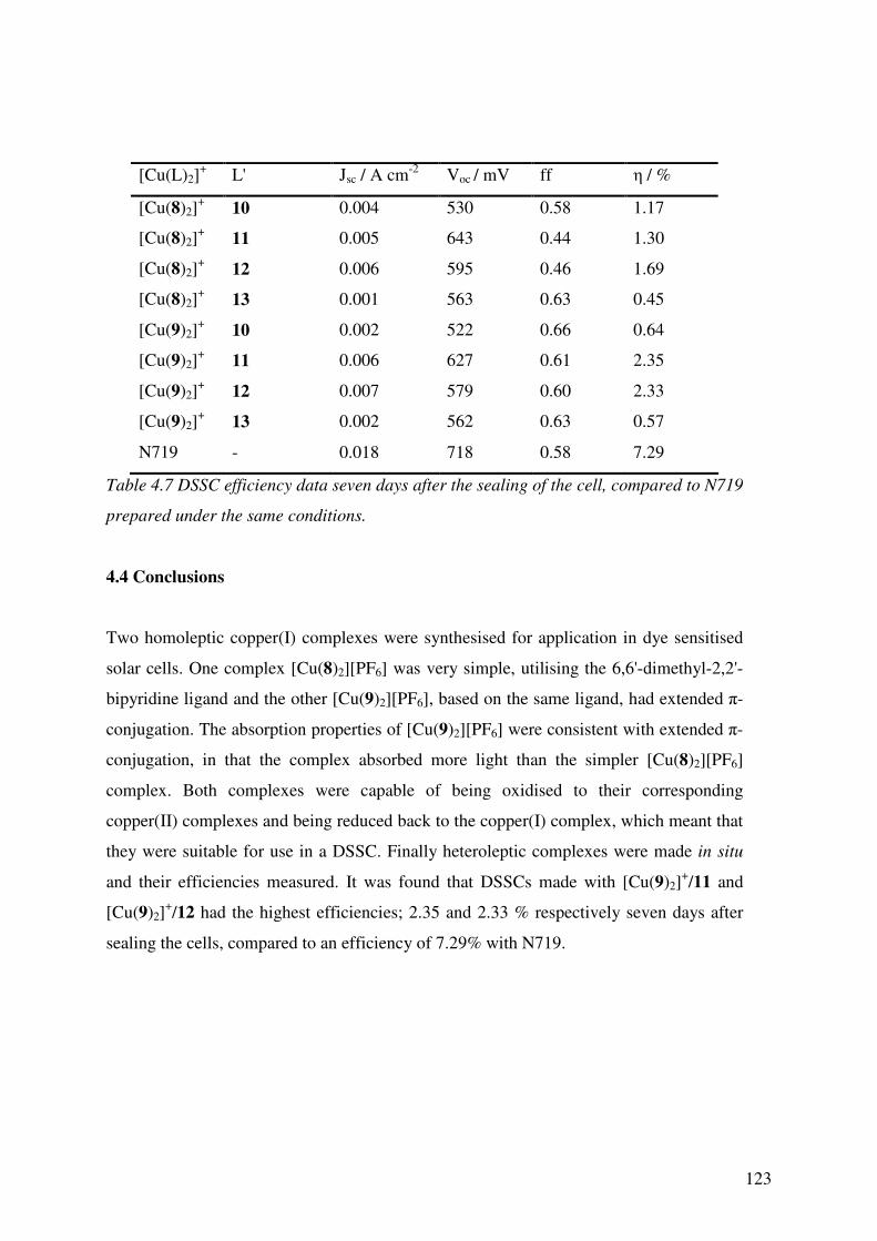
123

[Cu(L)2]+ L' Jsc / A cm-2 Voc / mV ff η / %

[Cu(8)2]+ 10 0.004 530 0.58 1.17

[Cu(8)2]+ 11 0.005 643 0.44 1.30

[Cu(8)2]+ 12 0.006 595 0.46 1.69

[Cu(8)2]+ 13 0.001 563 0.63 0.45

[Cu(9)2]+ 10 0.002 522 0.66 0.64

[Cu(9)2]+ 11 0.006 627 0.61 2.35

[Cu(9)2]+ 12 0.007 579 0.60 2.33

[Cu(9)2]+ 13 0.002 562 0.63 0.57

N719 - 0.018 718 0.58 7.29

Table 4.7 DSSC efficiency data seven days after the sealing of the cell, compared to N719

prepared under the same conditions.

4.4 Conclusions

Two homoleptic copper(I) complexes were synthesised for application in dye sensitised

solar cells. One complex [Cu(8)2][PF6] was very simple, utilising the 6,6'-dimethyl-2,2'-

bipyridine ligand and the other [Cu(9)2][PF6], based on the same ligand, had extended π-

conjugation. The absorption properties of [Cu(9)2][PF6] were consistent with extended π-

conjugation, in that the complex absorbed more light than the simpler [Cu(8)2][PF6]

complex. Both complexes were capable of being oxidised to their corresponding

copper(II) complexes and being reduced back to the copper(I) complex, which meant that

they were suitable for use in a DSSC. Finally heteroleptic complexes were made in situ

and their efficiencies measured. It was found that DSSCs made with [Cu(9)2]+/11 and

[Cu(9)2]+/12 had the highest efficiencies; 2.35 and 2.33 % respectively seven days after

sealing the cells, compared to an efficiency of 7.29% with N719.

124

4.5 Experimental

9

Synthesis:

Compound 8 (550 mg, 2.98 mmol) and 4-(diphenylamino)benzaldehyde (1.87 g,

6.87 mmol) were stirred in dry DMF (70 cm3) in a reaction flask and KOtBu (1.005g,

8.96 mmol) was added. The vessel was flushed with N2 for 10 min and the reaction

mixture was stirred for 56 h in the dark after which time a dark yellow solid precipitated.

This was filtered and dried in air. The crude product was dissolved in the minimum

amount of CH2Cl2 and purified by column chromatography (SiO2, CH2Cl2). The first

(orange) fraction was collected and solvent was removed in vacuo. Compound 9 was

isolated as a yellow powder

Yield: 1.13 g, 54.7%

1H NMR: (500 MHz, CDCl3, 25 ºC, TMS) δ/ppm: 8.41 (dd, J = 7.8, 0.6 Hz, 2H, A3),

7.81 (t, J = 7.8 Hz, 2H, A4), 7.73 (d, J = 16.0 Hz, 2H, b), 7.49 (dAB, J = 8.6 Hz, 2H, B2),

7.39 (dd, J = 7.7, 0.6 Hz, 2H, A5), 7.28 (m, 4H, C

3), 7.15 (m, 10H, C2+a),

7.07 (m, 8H, C4+B3).

13C NMR (126 MHz, CDCl3, 25 ºC, TMS) δ/ppm: 156.1 (A2), 155.3 (A6), 148.1 (B4),

147.6 (C1), 137.4 (A4), 132.4 (b), 130.8 (B1), 129.5 (C3), 128.2 (B2), 126.5 (a), 124.9

(C3), 123.4 (B3/C4), 123.3 (B3/C4), 121.9 (A5), 119.5 (A3).

ESI: m/z 695.3 [M + H]+ (calc. 695.3)

Found: C 85.49, H 5.64, N 7.96; C50H38N4·0.5H2O requires C 85.32, H 5.58, N 7.96.

Melting point: 241.4 °C

[Cu(8)2][PF6]

Synthesis:

[Cu(MeCN)4][PF6] (37.3 mg, 0.100 mmol) was dissolved in MeCN (2 cm3) and the

solution was added to a solution of compound 8 (36.8 mg, 0.200 mmol) in CHCl3

(5 cm3). The solution immediately became red in colour and was stirred for 30 min.

Addition of Et2O (10 cm3) afforded a red precipitate, which was collected by filtration

125

over Celite. The product was washed with H2O and Et2O and removed from the Celite by

dissolution in MeCN. Solvent was removed in vacuo and [Cu(8)2][PF6] was isolated as

red crystals.

Yield: 44.6 mg, 77.3%

1H NMR: (500 MHz, CD3CN, 25 ºC, TMS) δ/ppm: 8.26 (d, J = 8.0 Hz, 2H, A3),

8.02 (t, J = 7.9 Hz, 2H, A4), 7.50 (d, J = 7.7 Hz, 2H, A5), 2.22 (s, 6H, a) 13C NMR: δC (126 MHz, CD3CN, 25 ºC, TMS): 158.4 (A6), 152.6 (A2), 139.2 (A4),

126.7 (A5), 120.4 (A3), 25.2 (a).

MALDI-TOF: m/z 431.0 [M – PF6]+ (calc. 431.1), 246.5 [M – 8 – PF6]

+ (calc. 247.0).

Found: C 49.38, H4.18, N 9.63; C24H24N4CuPF6·0.5H2O requires

C 49.19, H15 4.30, N 9.56.

[Cu(9)2][PF6]

Synthesis: [Cu(MeCN)4][PF6] (26.8 mg, 0.0719 mmol) was dissolved in MeCN (2 cm3)

and the solution was added to a solution of 2 (100 mg, 0.14 mmol) in CHCl3 (10 cm3).

The solution immediately changed from yellow to orange and was ultrasonicated

for 60 min. The solvents were then removed in vacuo and [Cu(9)2][PF6] was isolated as

an orange powder.

Yield: 92.5 mg, 80.4 %

1H NMR: (500 MHz, CDCl3, 25 ºC, TMS) δ/ppm: 7.90 (d, J = 7.6, 4H, A3),

7.85 (t, J = 7.8 Hz, 4H, A4), 7.74 (d, J = 7.7 Hz, 4H, A5), 7.30 (t, J = 7.9 Hz, 16H, C3),

7.12 (d, J = 16.3 Hz, 4H, b), 7.08 (m, 24H, C2+C4), 6.79 (d, J = 8.6 Hz, 8H, B3)

overlapping with 6.77 (d, J = 16.3 Hz, 4H, a), 6.67 (d, J = 8.6 Hz, 8H, B2). 13C NMR: (126 MHz, CDCl3, 25 ºC, TMS) δ/ppm: 155.5 (A6), 152.2 (A2), 148.9 (B4),

147.1 (C1), 138.0 (A4), 135.0 (b), 129.6 (C3), 128.8 (B1), 127.9 (B2) 125.1 (C2),

124.7 (a), 123.9 (C4), 122.4 (A5), 122.3 (B3), 119.9 (A3).

ESI: m/z 1453.7 [M – PF6]+ (calc. 1452.6), 695.5 [2 + H]+ (calc. 695.3).

Found: C 73.98, H 4.76, N 7.71; C100H76CuF6N8P·MeCN·H2O requires

C73.92, H 4.93, N 7.61.

126

Preparation of Solar Cells:

TiO2 paste was prepared adapting the procedure of Grätzel and coworkers37; changes to

the published procedure were the use of a porcelain (in place of alumina) mortar,

sonicator bath in place of an ultrasonic horn, terpineol (CAS: 8000-41-7) rather than α-

terpineol, and the omission of the three roller mill treatment. The FTO glass (Solaronix

TCO22-7, 2.2 mm thickness, sheet resistance ≈7 Ω square–1) was cleaned by sonicating

in acetone, EtOH, Hellmanex® surfactant (2% in water), water and EtOH baths

sequentially for 10 min. After treatment in a UV-O3 system (Model 256-220, Jelight

Company Inc), the FTO plates were immersed in aqueous TiCl4 solution (40 mmol dm-3)

at 70ºC for 30 min, and washed with H2O and EtOH. Nanocrystalline TiO2 electrodes

were made by doctor blading the TiO2 paste onto a conducting glass slide and keeping

them at room temperature for 10 min to allow the paste to mature to minimize surface

irregularities. The electrode was then gradually heated under an air flow at 70°C for 30

min, 135°C for 5 min, 325°C for 5 min, 375°C for 90 min, 450°C for 15 min, and 500°C

for 15 min. After annealing, the TiO2 film was treated with 40 mM TiCl4 solution as

described above, rinsed with H2O and EtOH and sintered at 500°C for 30 min. After

cooling to ≈80°C, each electrode was immersed in a DMSO solution of anchoring ligand

10, 11, 12 or 13 (1 mmol dm–3) for 24 h. The colourless slide was removed from the

solution, washed with DMSO and EtOH, and dried. The electrode with adsorbed

anchoring ligand was immersed in an EtOH solution of [Cu(8)2][PF6] or a CH2Cl2

solution of [Cu(9)2][PF6] (0.4 mmol dm–3) and this was left to stand for 64 h during

which time the slide turned orange. The electrode was removed from the solution and

was washed with EtOH. To prepare the counter electrode, a hole was drilled in an FTO

glass plate (cleaned and pre-treated as above). The perforated sheet was heated in air for

15 min at 450°C to remove organic residues and was then washed as described for the

working electrode. The Pt catalyst was deposited on the FTO glass by coating with a drop

of H2PtCl6, 5 mmol dm–3 in propan-2-ol and heated to 400°C for 15 min. The dye-

covered TiO2 electrode and Pt counter-electrode were assembled using thermoplast hot-

melt sealing foil (Solaronix, Meltonix 1170-25 Series, 25 microns thick) by heating while

pressing them together. The electrolyte comprised LiI (0.1 mol dm–3), I2 (0.05 mol dm–3),

1-methylbenzimidazole (0.5 mol dm–3) and 1-butyl-3-methylimidazolinium iodide (0.6

mol dm–3) in methoxypropionitrile, and was introduced into the cell by vacuum

127

backfilling. The hole on the counter electrode was finally sealed using the hot-melt

sealing foil and a cover glass. Measurements were made by irradiating from behind using

a light source SolarSim 150 (100 mW cm–2 = 1 sun). The power of the simulated light

was calibrated by using a reference Si photodiode. The standard dye N719 was purchased

from Solaronix. The active area of the cell was 0.288 cm2 and the cell was not masked

during the measurements.

128

4.6 References

1. Kyoto Treaty, http://unfccc.int/kyoto_protocol/items/3145.php, Accessed 4th December, 2012.

2. A. Hagfeldt, G. Boschloo, L. Sun, L. Kloo and H. Pettersson, Chem. Rev., 2010, 110, 6595-6663.

3. M. Grätzel, J. Photochem. Photobiol. C, 2003, 4, 145-153. 4. S. Ardo and G. J. Meyer, Chem. Soc. Rev., 2009, 38, 115-164. 5. G. J. Meyer, ACS Nano, 2010, 4, 4337-4343. 6. M. K. Nazeeruddin, E. Baranoff and M. Grätzel, Sol. Energy, 2011, 85, 1172-

1178. 7. B. O'Regan and M. Gratzel, Nature, 1991, 353, 737-740. 8. Z. Yu, N. Vlachopoulos, M. Gorlov and L. Kloo, Dalton Trans., 2011, 40, 10289-

10303. 9. M. Grätzel, J. Photochem. Photobiol. C, 2003, 145-153. 10. M. K. Nazeeruddin, C. Klein, P. Liska and M. Grätzel, Coord. Chem. Rev., 2005,

249, 1460-1467. 11. M. K. Nazeeruddin, S. M. Zakeeruddin, J. J. Lagref, P. Liska, P. Comte, C.

Barolo, G. Viscardi, K. Schenk and M. Graetzel, Coord. Chem. Rev., 2004, 248, 1317-1328.

12. M. A. Green, K. Emery, Y. Hishikawa and W. Warta, Prog. Photovoltaics, 2008, 16, 435-440.

13. N. Alonso-Vante, J.-F. Nierengarten and J.-P. Sauvage, J. Chem. Soc. Dalton Trans., 1994, 1649-1654.

14. S. Sakaki, T. Kuroki and T. Hamada, J. Chem. Soc. Dalton Trans., 2002, 840-842. 15. T. Bessho, E. C. Constable, M. Graetzel, A. Hernandez Redondo, C. E.

Housecroft, W. Kylberg, M. K. Nazeeruddin, M. Neuburger and S. Schaffner, Chem. Commun., 2008, 3717-3719.

16. E. C. Constable, A. H. Redondo, C. E. Housecroft, M. Neuburger and S. Schaffner, Dalton Trans., 2009, 6634-6644.

17. C. L. Linfoot, P. Richardson, T. E. Hewat, O. Moudam, M. M. Forde, A. Collins, F. White and N. Robertson, Dalton Trans., 2010, 39, 8945-8956.

18. B. Bozic-Weber, E. C. Constable, C. E. Housecroft, M. Neuburger and J. R. Price, Dalton Trans., 2010, 39, 3585-3594.

19. B. Bozic-Weber, E. C. Constable, C. E. Housecroft, P. Kopecky, M. Neuburger and J. A. Zampese, Dalton Trans., 2011, 40, 12584-12594.

20. W. L. Parker and G. A. Crosby, J. Phys. Chem., 1989, 93, 5692-5696. 21. T. Maruyama and T. Yamamoto, Inorg. Chim. Acta, 1995, 238, 9-13. 22. L. Allouche, A. Marquis and J.-M. Lehn, Chem. Eur. J., 2006, 12, 7520-7525. 23. P. J. Burke, D. R. McMillin and W. R. Robinson, Inorg. Chem., 1980, 19, 1211-

1214. 24. S. Itoh, N. Kishikawa, T. Suzuki and H. D. Takagi, Dalton Trans., 2005, 1066-

1078. 25. S. Kitagawa, M. Munakata and A. Higashie, Inorg. Chim. Acta, 1984, 84, 79-84. 26. Z. A. Siddique, Y. Yamamoto, T. Ohno and K. Nozaki, Inorg. Chem., 2003, 42,

6366-6378.

129

27. V. Tamilavan, N. Cho, C. Kim, J. Ko and M. H. Hyun, Tetrahedron, 2012, 68, 5890-5897.

28. J. Jia, K. Cao, P. Xue, Y. Zhang, H. Zhou and R. Lu, Tetrahedron, 2012, 68, 3626-3632.

29. W. Fan, D. Tan and W.-Q. Deng, ChemPhysChem, 2012, 13, 2051-2060. 30. P. Péchy, T. Renouard, S. M. Zakeeruddin, R. Humphry-Baker, P. Comte, P.

Liska, L. Cevey, E. Costa, V. Shklover, L. Spiccia, G. B. Deacon, C. A. Bignozzi and M. Grätzel, J. Am. Chem. Soc., 2001, 123, 1613-1624.

31. M. Yamada, K. Araki and S. Shiraishi, B. Chem. Soc. Jpn., 1988, 61, 2208-2210. 32. U. B. Cappel, E. A. Gibson, A. Hagfeldt and G. Boschloo, J. Phys. Chem. C, 2009,

113, 6275-6281. 33. A. L. Spek, Acta Crystallogr. D, 2009, 65, 148-155. 34. B. Wenger, M. Grätzel and J.-E. Moser, Chimia, 2005, 59, 123-125. 35. V. K. Thorsmølle, B. Wenger, J. Teuscher, C. Bauer and J.-E. Moser, Chimia,

2007, 61, 631-634. 36. B. Wenger, M. Grätzel and J.-E. Moser, J. Am. Chem. Soc., 2005, 127, 12150-

12151. 37. S. Ito, P. Chen, P. Comte, M. K. Nazeeruddin, P. Liska, P. Péchy and M. Grätzel,

Prog. Photovoltaics, 2007, 15, 603-612.

130

Chapter 5

A DFT and TD-DFT investigation of copper(I) polypyridyl complexes with

application in DSSCs

5.1 Introduction

Copper(I) complexes are a promising, cheap option to potentially use as sensitisers in dye

sensitised solar cells (DSSCs)1, 2. Homoleptic complexes containing suitable anchoring

ligands have shown reasonable efficiencies in DSSCs3-5 but in order to incorporate both

anchoring groups into the complex and allow the properties to be tuned, the use of

heteroleptic complexes offers greater flexibility6, 7. Heteroleptic complexes can be made

by attaching an anchoring ligand to nanoparticles of titanium dioxide (TiO2, anatase) and

then placing the TiO2 into a solution of a homoleptic copper(I) complex. This leads to the

formation of a heteroleptic complex, attached to the surface of the TiO2. There is

however a problem with this approach; due to the lability of Cu(I), a statistical mixture of

heteroleptic and homoleptic complexes will be present in solution around the TiO2. It is

not possible to isolate and characterise the heteroleptic complex. The only current means

of characterising this heteroleptic complex is as the surface-bound species by means of

solid state absorption spectroscopy and mass spectrometry6. Therefore, the properties of

such a complex are currently not well understood.

DFT and TD-DFT have been used to investigate ruthenium-based sensitisers for DSSCs,

examining both structural and electronic properties of the dye in question and probing the

transitions making up its absorption spectrum.

The first notable study was carried out by Fantacci et al. in 2003 in a first principles

investigation of the dye N3 (Fig. 5.1)8.

Fig. 5.1 The cis- and trans-structures of the N3 dye.

131

In order to validate the studies, the optimised geometries of the two stereoisomers of the

complexes were compared to experimental crystallographic data. The agreement between

the experimental and calculated data was good, verifying the choice of method and basis

set. The highest occupied molecular orbital HOMO, (HOMO−1) and (HOMO−2) orbitals

were found to be quasi-degenerate and predominantly localised on the thiocyanate

(SCN-) ligands with minor contributions from the ruthenium d-orbitals. The (HOMO−4),

(HOMO−5) and (HOMO−6) were localised on the metal atom whilst the LUMO to

(LUMO+5) orbitals were based on the bipyridine ligands with substantial contributions

from the carboxylic acid groups. This is favourable for injection of an electron into TiO2

on excitation of the molecule. Using TD-DFT the predicted shape of the absorption bands

and the separation of said bands was in reasonable agreement with experimental data,

although the prediction of the specific positions of the bands was limited.

In 2006 Barolo et al. investigated a ruthenium complex with a tetradentate ligand, N886

(Fig 5.2)9. Although the complex was characterised experimentally with 4'-tbutyl

substituents, these were replaced by methyl substituents for computational convenience.

N

N

COOH

N

N

HOOC

Ru

NCS

SCN

Fig. 5.2 The structure of the N886 dye, with tBu substituents replaced with methyl groups

The calculations focussed on the effect of deprotonation of the carboxylic acid groups on

the energy levels of the HOMO and LUMO of the complex and it was found that

deprotonation of the –COOH groups led to greater destabilisation of the LUMO rather

than the HOMO. The HOMO and nHOMOs (next HOMOs) possessed ruthenium d-

orbital and thiocyanate character whereas the LUMO and nLUMOs (next LUMOs) were

localised on the quaterpyridine (qpy) ligand, specifically the pyridine moieties with

carboxylic acid substituents. Using TD-DFT to calculate the absorption spectrum of the

di-protonated complex resulted in very good (within 15 nm) agreement with experimental

132

data, except in the case of the lowest-energy band. This band was predicted at 699 nm

and observed experimentally at 637 nm. The transition is the result of electron promotion

from a mixed ruthenium-thiocyanate orbital to an orbital based on the qpy ligand9. A

higher energy band also involves promotion to an orbital based on the qpy ligand. The

HOMO and LUMO of a Ti38O72 cluster were also calculated and compared to the energy

levels of the dye to explore how favourable the injection of an electron from the dye into

the TiO2 was.

A similar study was carried out by Nazeeruddin et al in 2007 on the dye N945 (Fig. 5.3)10.

N

N

Ru

SCNNCS

N

N

COOH

HOOC

O

O

O

O

Fig. 5.3 The structure of the N945 dye.

It was found that the HOMO, (HOMO−1) and (HOMO−2) all had ruthenium d-orbital

character, with significant contribution from the thiocyanate ligands. The LUMO and

(LUMO+2) were localised on the carboxylic acid substituted bipyridine and the

(LUMO+1) and (LUMO+3) were localised on the other bipyridine ligand. The energy

levels of the orbitals were also calculated and compared to previous results for a model

TiO2 nanoparticle. The results suggested that the LUMO and LUMO+1 were of a suitable

energy match with the conductance band edge of TiO2 for favourable electron injection.

This was corroborated experimentally as high photocurrents were measured.

DFT and TD-DFT studies have also been carried out on Cu(I) complexes. In 2010

Robertson and coworkers investigated the properties of four heteroleptic Cu(I) complexes

(Fig. 5.4) of which one was then used in a DSSC7.

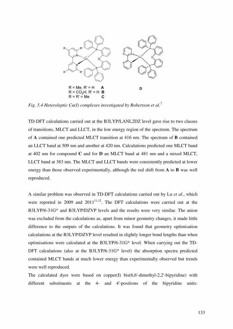
133

P

O

P

Cu

N

N

R'

R'

R

R

R = Me, R' = H A

R = CO2H, R' = H B

R = R' = Me C

Fig. 5.4 Heteroleptic Cu(I) complexes investigated by Robertson et al.7

TD-DFT calculations carried out at the B3LYP/LANL2DZ level gave rise to two classes

of transitions, MLCT and LLCT, in the low energy region of the spectrum. The spectrum

of A contained one predicted MLCT transition at 416 nm. The spectrum of B contained

an LLCT band at 509 nm and another at 420 nm. Calculations predicted one MLCT band

at 402 nm for compound C and for D an MLCT band at 481 nm and a mixed MLCT,

LLCT band at 383 nm. The MLCT and LLCT bands were consistently predicted at lower

energy than those observed experimentally, although the red shift from A to B was well

reproduced.

A similar problem was observed in TD-DFT calculations carried out by Lu et al., which

were reported in 2009 and 201111,12. The DFT calculations were carried out at the

B3LYP/6-31G* and B3LYP/DZVP levels and the results were very similar. The anion

was excluded from the calculations as, apart from minor geometry changes, it made little

difference to the outputs of the calculations. It was found that geometry optimisation

calculations at the B3LYP/DZVP level resulted in slightly longer bond lengths than when

optimisations were calculated at the B3LYP/6-31G* level. When carrying out the TD-

DFT calculations (also at the B3LYP/6-31G* level) the absorption spectra predicted

contained MLCT bands at much lower energy than experimentally observed but trends

were well reproduced.

The calculated dyes were based on copper(I) bis(6,6'-dimethyl-2,2'-bipyridine) with

different substituents at the 4- and 4'-positions of the bipyridine units:

P

O

P

Cu

N N

N N

D

134

• Ethenyl groups to add conjugation

• Carboxylic acid or ester groups to look at protonation effects

• Heteroaromatic groups such as selenophene, furan and thiophene to adjust

molecular orbital energies and compositions.

It was found the enhancing π-conjugation destabilises HOMOs and stabilises LUMOs

and that the introduction of heteroaromatic groups stabilises HOMOs much more than

LUMOs as the HOMO is based not only on the copper atom but also on the

heteroaromatic-substituted ligand.

In order to minimise the synthesis of multiple dyes, which is both expensive and time-

consuming, the aim of this chapter is to demonstrate that DFT and TD-DFT can be used

to develop a method of screening multiple heteroleptic copper(I) complexes which could

be used in DSSCs. In order to validate the method used theoretical data for the

homoleptic complexes will be compared to experimental data. The heteroleptic

complexes will then be calculated and the results rationalised in terms of efficiencies in

DSSCs.

In this study, the following homoleptic complexes have been investigated (Fig. 5.5).

Fig. 5.5 The homoleptic complexes studied, (left) [Cu(8)2]+, (right) [Cu(9)2]

+. The

counter-anions were omitted from the calculations.

5.2 Calculation Details

The DFT calculations were carried out as follows: For [CuL2]+ (L = 8 or 9), the TD-DFT

calculations were based upon known crystallographic data (this work). For [CuLL']+ (L =

135

8 or 9, L' = 10-12) calculations were started from optimised structures of [Cu(8)2]+ and

[Cu(9)2]+ and were computationally modified. Initial energy optimisation was carried out

at the Hartree-Fock (HF) level with a 3-21G* basis set, followed by HF/6-31G*.

Frequency calculations were carried out at this level to confirm that a minimum energy

had been achieved. The structures were further relaxed with the hybrid 3-parameter Lee-

Yang-Parr functional13, 14 B3LYP/6-31G*. To account for solvent effects, the conductor-

like polarisable continuum model15, 16 (CPCM) was used. The CPCM was used in

geometry optimisation and for subsequent TD-DFT calculations.

As many of the calculations are computationally demanding, the influence of a

considerably larger basis set (6-311++G**) was assessed by alternatively using an

extended basis set on either the metal atom or on all ligand atoms. For the smaller

complexes the entire calculation was also carried out with the 6-311++G** basis set

throughout. Explorative calculations were also carried out with a LANL2DZ basis set on

the Cu atom and 6-31G* for the remaining system. Predicted electronic transitions were

calculated at the B3LYP level and simulated spectra were generated from the Gaussian

09 output using the GaussSum program, version 2.217.

The conversion factor from Hartree to eV is 1 Eh = 27.21128505 eV, taken from the

NIST website 2010 values18. All calculations were carried out using the Gaussian 09

program package19.

5.3 Results and Discussion

In order to validate the geometry optimisations, the calculated structures were compared

to experimentally obtained crystallographic structures (this work) (Table 5.1).

136

Parameter [Cu(8)2]+

(DFT) [Cu(8)2]

+ (expt)

[Cu(9)2]+

(DFT) [Cu(9)2]

+ (expt)

Cu1–N1 / Å 2.004 2.0248(9) 2.020 2.038(2)

Cu1–N2 / Å 2.004 2.0472(9) 2.020 2.038(2)

Cu1–N3 / Å 2.004 2.0447(9 2.020 2.038(2)

Cu1–N4 / Å 2.004 2.0335(9) 2.020 2.038(2)

N1–Cu1–N2 / o 82.92 81.13(4) 83.06 80.48(6)

N1–Cu1–N3 / o 124.24 127.51(4) 131.56 125.64(6)

N2–Cu1– N3 / o 124.24 114.67(4) 131.56 125.64(6)

N1–Cu1– N4 / o 124.17 125.93(4 131.56 125.64(6)

N2–Cu1–N4 / o 124.11 132.08(4) 131.56 125.64(6)

N3–Cu1–N4 / o 82.92 81.59(3) 83.06 80.48(6)

Table 5.1 Comparison of DFT and single crystal X–ray structural parameters for the

coordination spheres in [Cu(8)2]+ and [Cu(9)2]

+. Atom numbering corresponds to Figs.

4.33 and 4.39, experimental data are from chapter 4.

Although the Cu1-Nx (x = 1-4) bond lengths were slightly underestimated by the

calculations, the geometries calculated using DFT were still realistic. The absorption

spectra of the complexes were then calculated and the results compared with

experimental data.

0

200 300 400 500 600

Wavelength (nm)

Ab

so

rban

ce (

a.u

.)

Experimental

Calculated (6-31G*)

Fig. 5.6 Calculated (6-31G* basis set) versus experimental electronic absorption spectra

of [Cu(8)2]+

in acetonitrile. The first fifty transitions were calculated. The figure was

generated using the output of the GaussSum program17

.

137

The agreement in the high energy region of the spectrum is good (Fig. 5.6). However, the

TD calculations predict two MLCT bands in the visible region with λmax = 378, 532 nm,

which are not observed experimentally. The band at 378 nm has two components,

(HOMO-1) → (LUMO+2) and HOMO → (LUMO+3). The transition at 532 nm has two

major components and these are depicted in Fig. 5.7.

Fig. 5.7 The components of the MLCT band with λmax = 532 nm in [Cu(8)2]

+.

The (HOMO−1) is predominantly metal based with some contribution from the pyridine

rings. The LUMO and (LUMO+1) are predominantly ligand-based with some Cu d-

orbital involvement. Whilst the band centered at 378 nm may be rationalised as

corresponding to the tail of the experimentally observed band at 312 nm, the calculated

band centered at 532 nm is 80 nm red-shifted with respect to the experimentally observed

band with λmax = 460 nm. The over-estimation of the MLCT red-shift is also observed in

reports by Lu et al.11, 12.

The absorption spectrum of [Cu(9)2]+ was also calculated using TD-DFT (Fig. 5.8) and

the agreement between the experimental and calculated spectra was better than that

obtained for [Cu(8)2]+, the smallest basis set (6-31G*) was used.

138

0

250 300 350 400 450 500 550 600 650

Wavelength (nm)

Ab

so

rban

ce (

a.u

.).

Experimental

Calculated (6-31G*)

Fig. 5.8 Calculated (6-31G* basis set) versus experimental electronic absorption spectra

of [Cu(9)2]+

in acetonitrile. The first fifty transitions were calculated. The figure was

generated using the output of the GaussSum program17

.

The lowest energy absorption in the experimental spectrum has λmax = 390 nm and the

TD calculation predicts a spectrum with a band at λmax = 435 nm. The calculated and

experimental spectra, therefore, are in tolerable agreement with one another, compared to

some reports of ruthenium polypyridyl complexes where the predicted and calculated

absorption spectra differ by up to 100 nm8, 10, 20, 21.

In order to obtain more accurately predicted UV-vis spectra a larger basis set was

employed. Diffuse functionals were also added to the calculations as electron density is

generally more spread out over molecules in the excited state. Starting from the geometry

optimised structures using the 6-31G* basis set the geometry was further optimised using

the 6-311++G** basis set in the presence of acetonitrile by means of the CPCM.

The TD-DFT calculations were then also carried out using the 6-311++G** basis set,

also including the CPCM (Fig. 5.9).

139

0

200 250 300 350 400 450 500 550 600 650

Wavelength (nm)

Ab

so

rba

nc

e (

a.u

.) Experimental

6-31G* on all atoms

6-311++G** on all atoms

Fig. 5.9 Calculated versus experimental electronic absorption spectra of [Cu(8)2]+

in

acetonitrile. The first fifty transitions were calculated. The figure was generated using the

output of the GaussSum program17

.

As for the calculation with the 6-31G* basis set, the agreement between the predicted and

experimental spectra in the high energy region of the spectra is good. In the visible region

the accuracy is much improved by using the 6-311G** basis set; only one MLCT band is

predicted and it is red-shifted by 29 nm (λmax = 489 nm) with respect to the experimental

peak (λmax = 460 nm). However, using such a large basis set is computationally intensive

and time-consuming. Whilst it is feasible for a small molecule such as [Cu(8)2]+, this is

not the case for larger molecules. Therefore, a split basis set employing the 6-311++G**

basis set to describe the copper atom and the 6-31G* basis set to describe the carbon,

hydrogen and nitrogen atoms was used. Starting from the geometry optimised structures

using the 6-31G* basis set the geometry was further optimised using the split basis set (6-

311++G** on Cu and 6-31G* on C, H, N) in the presence of acetonitrile by means of the

CPCM. The TD-DFT calculations were also carried out using the split basis set and

including the solvent model (Fig. 5.10).

140

0

200 250 300 350 400 450 500 550 600 650

Wavelength (nm)

Ab

so

rba

nc

e (a

.u)

Experimental

6-31G* on all atoms

6-311++G** on all atoms

6-311++G** on Cu, 6-31G* on C,H,N

Fig. 5.10 Calculated versus experimental electronic absorption spectra of [Cu(8)2]+

in

acetonitrile. The first fifty transitions were calculated. The figure was generated using the

output of the GaussSum program17

.

The agreement between the calculated and experimental spectra improved again on

employment of the split (6-311++G**/6-31G*) basis set. One MLCT transition centered

at 470 nm is predicted, which is red-shifted by 10 nm compared to the experimental

spectrum (λmax = 460 nm). The MLCT transition has four components which are depicted

in Fig. 5.11, and involves the orbitals (HOMO−1), HOMO, LUMO and (LUMO+1).

141

Fig. 5.11 The components of the calculated MLCT band at 470 nm for [Cu(8)2]+ (basis

set: 6-311++G** on Cu and 6-31G* on the ligand atoms). Isodensity surfaces for the

MOs were generated from the Kohn-Sham orbitals using the MOLEKEL program22

.

The character of the orbitals changes very little on altering the basis set. The HOMO and

(HOMO−1) have predominantly Cu d-orbital character, with some contribution from the

pyridine rings, particularly the nitrogen atoms. The LUMO and (LUMO+1) are

essentially ligand based.

One further possibility for calculating the absorption spectra for these types of complexes

is the use of the split basis set LANL2DZ23/6-31G*. The spectrum of [Cu(8)2]+ was

calculated using this split basis set and the result was very similar to that obtained from

using 6-311++G**/6-31G* (Fig. 5.12).

142

0

200 250 300 350 400 450 500 550 600 650

Wavelength (nm)

Ab

so

rba

nc

e (

a.u

)Experimental

6-311++G** on Cu, 6-31G* on C,H,N

LANL2DZ on Cu, 6-31G* on C, H, N

Figure 5.12. Predicted absorption spectra for [Cu(8)2]+ showing that use of the

LANL2DZ/6-31G* basis set is as good as the use of the 6-311++G**/6-31G* basis set.

The LANL2DZ/6-31G* calculation predicts an MLCT λmax that is slightly blue-shifted,

compared to experiment and the 6-311++G**/6-31G* calculation predicts an MLCT λmax

that is slightly red-shifted compared to experiment. Both calculations reproduce the high

energy absorptions well.

It is concluded that the electronic absorption spectrum of [Cu(8)2]+ can be realistically

captured using either the LANL2DZ/6-31G* or the 6-311++G**/6-31G* split basis set.

The absorption spectrum of [Cu(9)2]+ was predicted using the split basis set

(6-311++G** on Cu, 6-31G* on C, H and N) and the results are depicted in Fig. 5.13.

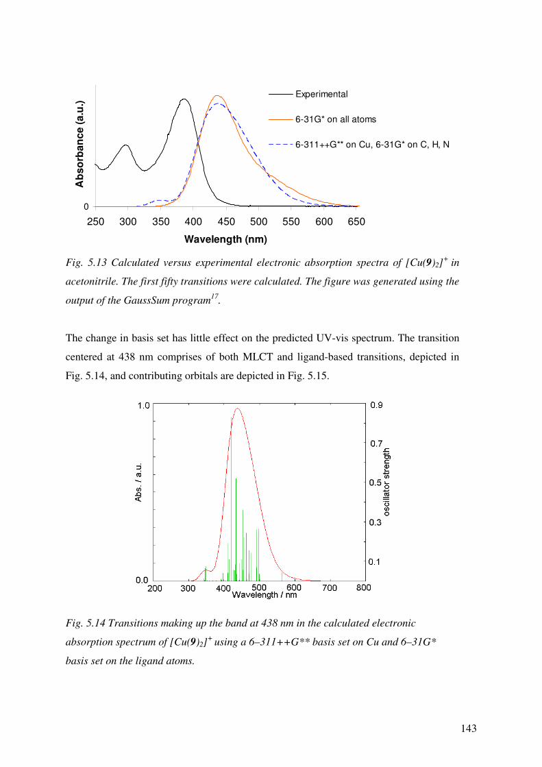
143

0

250 300 350 400 450 500 550 600 650

Wavelength (nm)

Ab

so

rba

nc

e (

a.u

.)

Experimental

6-31G* on all atoms

6-311++G** on Cu, 6-31G* on C, H, N

Fig. 5.13 Calculated versus experimental electronic absorption spectra of [Cu(9)2]+

in

acetonitrile. The first fifty transitions were calculated. The figure was generated using the

output of the GaussSum program17

.

The change in basis set has little effect on the predicted UV-vis spectrum. The transition

centered at 438 nm comprises of both MLCT and ligand-based transitions, depicted in

Fig. 5.14, and contributing orbitals are depicted in Fig. 5.15.

Fig. 5.14 Transitions making up the band at 438 nm in the calculated electronic

absorption spectrum of [Cu(9)2]+

using a 6–311++G** basis set on Cu and 6–31G*

basis set on the ligand atoms.

144

Fig. 5.15 Molecular orbitals (MOs) that contribute to the transitions that make up the

calculated MLCT band at 438 nm for [Cu(9)2]+ (basis set: 6-311++G** on Cu and 6-

31G* on the ligand atoms). Isodensity surfaces for the MOs were generated from the

Kohn-Sham orbitals using the MOLEKEL program22

.

The majority of the molecular orbitals are predominantly ligand-based, accounting for the

similarities in the photophysical and electrochemical properties of the ligand and the

complex. Dominance of the triphenylamine moeties’ contribution to the HOMO and

(HOMO–1) supports the findings from the spectroelectrochemistry (§ 4.3.6).

As the level of agreement between the experimental and calculated data is satisfactory for

both complexes [Cu(L)2]+ (L = 8, 9) TD-DFT calculations were carried out for

heteroleptic complexes of the type [Cu(L)(L')]+ where L = 8, 9 and L' = 10-12 (see Fig

5.16 for structures of 10-12), using the split 6-311++G**/6-31G* basis set.

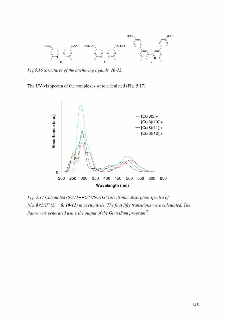
145

Fig 5.16 Structures of the anchoring ligands, 10-12.

The UV-vis spectra of the complexes were calculated (Fig. 5.17)

0

200 250 300 350 400 450 500 550 600 650

Wavelength (nm)

Ab

so

rba

nc

e (

a.u

.) [Cu(8)2]+

[Cu(8)(10)]+

[Cu(8)(11)]+

[Cu(8)(12)]+

Fig. 5.17 Calculated (6-311++G**/6-31G*) electronic absorption spectra of

[Cu(8)(L')]+ (L' = 8, 10-12) in acetonitrile. The first fifty transitions were calculated. The

figure was generated using the output of the GaussSum program17

.

146

Complex λmax/nm Orbital Contributions

[Cu(8)2]+ 470 45% LUMO←(HOMO–1)

40% (LUMO+1)←HOMO

7% (LUMO+1)←(HOMO–1)

7% LUMO←HOMO

[Cu(8)(10)]+ 504

86% LUMO←HOMO

12% (LUMO+1)←(HOMO–1)

418 97% LUMO←HOMO

[Cu(8)(11)]+ 486

81% LUMO←HOMO

15% (LUMO+1)←(HOMO–1)

382 91% (LUMO+2)←HOMO

4% LUMO←(HOMO–3)

[Cu(8)(12)]+ 491

71% LUMO←HOMO

16% (LUMO+1)←(HOMO–1)

7% LUMO←(HOMO–1)

3% (LUMO+3)←HOMO

414 77% (LUMO+2)←HOMO

19% (LUMO+2)←(HOMO–1)

Table 5.2 Orbital contributions to the electronic absorption transitions making up the

MLCT band in the visible region for [Cu(8)2]+ and [Cu(8)(L')]+

(L' = 10-12).

For all of the heteroleptic complexes [Cu(8)(L')]+ the HOMOs have predominantly

copper d-orbital character with some minor contribution from the pyridine rings (Figs.

5.18 and 5.19).

147

Fig. 5.18 Highest occupied MO involved in transitions contributing to the calculated

absorption spectra of [Cu(8)(10)]+ (right), [Cu(8)(11)]

+ (centre), and [Cu(8)(12)]

+ (left).

The (HOMO−1) orbitals are also predominantly metal based, except in the case of

[Cu(8)(10)]+ where there is significant contribution from ligand 8. This is also the case

for the (HOMO−3) orbital of [Cu(8)(11)]+.

Fig. 5.19 Second highest occupied MO involved in transitions contributing to the

calculated absorption spectra of [Cu(8)(10)]+ (right), [Cu(8)(11)]

+ (centre), and

[Cu(8)(12)]+ (left).

The LUMO and (LUMO+1) orbitals of the complex [Cu(8)(10)]+ are unexpectedly both

metal- and ligand-based (Fig. 5.20). For favourable injection of an electron from the

molecule in its excited state into the conductance band of TiO2, the LUMO should lie on

the anchoring ligand (ligand 10 for this complex). As this is not the case, a poorer

148

efficiency would be expected from a DSSC incorporating [Cu(8)(10)]+ as the sensitiser.

This is validated by experiment (Table 5.3).

[CuL2]+ L' ISC / A cm–2

VOC / V ff η / %

[Cu(8)2]+ 10 0.004 0.530 0.58 1.17

[Cu(8)2]+ 11 0.005 0.643 0.44 1.30

[Cu(8)2]+ 12 0.006 0.595 0.46 1.69

N719 - 0.018 0.718 0.58 7.29

Table 5.3 DSSC efficiency data seven days after sealing. The [Cu(8)2]+ complex is

introduced for surface exchange as the [PF6]- salt.

Fig 5.20 Lowest unoccupied MOs involved in transitions contributing to the calculated

absorption spectrum of [Cu(8)(10)]+, LUMO+1 (left), LUMO (right). The anchoring

ligand 10 is at the top of each graphic.

In complex [Cu(8)(11)]+, the LUMO and (LUMO+2) orbitals are localised on the

anchoring ligand, 11 (Fig. 5.21). The (LUMO+1) is localised on ligand 8 but as

contribution of the transition (HOMO−1)→(LUMO+1) is small this should not greatly

affect the efficiency of a DSSC incorporating this dye.

149

Fig 5.21 Lowest unoccupied MOs involved in transitions which contribute to the

calculated absorption spectrum of [Cu(8)(11)]+. The anchoring ligand 11 is at the top of

each graphic. (LUMO+2) (left), (LUMO+1) (centre),and LUMO (right).

For complex [Cu(8)(12)]+ all of the unoccupied molecular orbitals involved in transitions

contributing to the MLCT bands are localised on the anchoring ligand (Fig. 5.22). This

indicates that the dye is a potential candidate for use as a sensitiser in DSSCs.

Fig 5.22 Lowest unoccupied MOs involved in transitions which contribute to the

calculated absorption spectrum of [Cu(8)(12)]+. The anchoring ligand 12 is at the top of

each graphic. LUMO+2 (left), LUMO+1 (centre), and LUMO (right).

The efficiencies of the cells follow the same trend as the orbital contribution to the

complexes. The higher the proportion of unoccupied molecular orbital localised on the

150

anchoring ligand, the greater the efficiency of the DSSC (Table 5.3). This gives a basis

for screening complexes in silico before synthesis so that only dyes which have a large

proportion of the unoccupied electron density on the anchoring ligands are made for use

in DSSCs.

The UV-vis spectra of the heteroleptic complexes using 9 were also calculated (Fig. 5.23).

The spectra are more complicated than those of complexes incorporating ligand 8 as the

band in the visible region of the spectrum is made up of multiple transitions.

0

250 300 350 400 450 500 550 600 650

Wavelength (nm)

Ab

so

rba

nc

e (

a.u

.)

[Cu(9)(10)]+

[Cu(9)(11)]+

[Cu(9)(12)]+

Fig. 5.23 Calculated (6-311++G**/6-31G*) electronic absorption spectra of

[Cu(9)(L’)]+

(L’ = 10-12) in acetonitrile. The first fifty transitions were calculated. The

figure was generated using the output of the GaussSum program17

.

All three spectra predict two absorption bands, the first in the UV region of the spectrum

and the second in the visible region. For all complexes the band centred around 435 nm is

the result of multiple MLCT and LLCT transitions. The orbitals involved in transitions

for [Cu(9)(10)]+, [Cu(9)(11)]+ and [Cu(9)(12)]+ are depicted in Figs. 5.24, 5.25 and 5.26

respectively. (For transition tables see appendix)

151

LUMO+3

LUMO+2

LUMO+1

LUMO

HOMO

HOMO–1

HOMO–2

HOMO–3

HOMO–4

HOMO–5

HOMO–6

Fig 5.24 Highest occupied and lowest unoccupied MOs in [Cu(9)(10)]+. The anchoring

ligand 10 is at the bottom of each graphic.

The (HOMO−6) orbital is the only occupied molecular orbital which participates in

transitions and has predominantly metal character. The (HOMO−5), (HOMO−4) and

(HOMO−1) orbitals are based on the anchoring ligand and the (HOMO−3) and

(HOMO−2) orbitals are located on 9. Both the HOMO and the LUMO orbitals are

centred on the triphenylamine unit of 9, as is the (LUMO+3). The (LUMO+1) resides

mainly on the bipyridine moiety of 9 and the only LUMO character residing on the

anchoring ligand is that of (LUMO+2). This is not favourable for electron injection into

152

TiO2 when the dye is used in DSSCs. Correspondingly; this complex shows a poor

efficiency when used in a solar cell (Table 5.4).

LUMO+4

LUMO+3

LUMO+2

LUMO+1

LUMO

HOMO

HOMO–1

HOMO–2

HOMO–3

HOMO–4

HOMO–5

HOMO–6

Fig 5.25 Highest occupied and lowest unoccupied MOs in [Cu(9)(11)]+. The anchoring

ligand 11 is at the bottom of each graphic.

Both (HOMO−6) and (HOMO−5) have predominantly 9 character with some

contribution from the metal d-orbitals. The (HOMO−4) is predominantly based on 9, in

contrast to the (HOMO−3) and (HOMO−2), which are predominantly metal based. Both

(HOMO−1) and the HOMO are spread over half of ligand 9, in a similar manner to that

153

of (LUMO+2) and (LUMO+3). The LUMO and (LUMO+4) orbitals reside on the

anchoring ligand, 11 and the (LUMO+1) orbital resides on the bipyridine unit of 9. Use

of this complex in a DSSC results in an efficiency of 2.35% (Table 5.4), which is the best

efficiency of all the dyes described in this chapter.

LUMO+5

LUMO+4

LUMO+3

LUMO+2

LUMO+1

LUMO

HOMO

HOMO–1

HOMO–2

HOMO–3

HOMO–4 HOMO–5

Fig 5.26 Highest occupied and lowest unoccupied MOs in [Cu(9)(12)]+. The anchoring

ligand 12 is at the bottom of each graphic.

154

The (HOMO−5), (HOMO−3) and (HOMO−2) orbitals have predominantly copper

d-orbital character with minor contributions from the pyridine rings. The (HOMO−4),

(HOMO−1) and HOMO are all ligand 9 based. The LUMO, (LUMO+2) and (LUMO+5)

orbitals all reside on the anchoring ligand and, correspondingly, a good efficiency of

2.33% is observed when this complex is used in a DSSC. The (LUMO+1) and

(LUMO+4) are based on the bipyridine unit of 9 and (LUMO+3) is delocalised over half

of ligand 9.

[CuL2]+ L' ISC / A cm–2

VOC / V ff η / %

[Cu(9)2]+ 10 0.002 0.522 0.66 0.64

[Cu(9)2]+ 11 0.006 0.627 0.61 2.35

[Cu(9)2]+ 12 0.007 0.579 0.60 2.33

N719 - 0.018 0.718 0.58 7.29

Table 5.4 DSC efficiency data 7 days after sealing, compared to standard dye N719

measured under the same conditions. [Cu(9)2]+ is introduced for surface ligand

exchange as the [PF6]- salt.

Complex HOMO-LUMO gap / eV

Complex HOMO-LUMO gap / eV

[Cu(8)2]+ 3.42

[Cu(9)2]

+ 2.87

[Cu(8)(10)]+ 2.87 [Cu(9)(10)]+ 0.23 [Cu(8)(11)]+ 3.17 [Cu(9)(11)]+ 2.60 [Cu(8)(12)]+ 3.11 [Cu(9)(12)]+ 2.66

Table 5.5 Calculated HOMO-LUMO gaps for [Cu(8)(L')]+ (L' = 8, 10, 11, 12) and

[Cu(9)(L')]+ (L' = 9, 10, 11, 12). The conversion factor from Hartrees to eV was

1 Eh = 27.21128505 eV, taken from the NIST website 2010 values18

.

The HOMO-LUMO gaps for the homoleptic and heteroleptic complexes are compared in

Table 5.5. The energy gap is reduced on going from [Cu(8)2]+ to [Cu(9)2]

+, and the same

trend is observed between pairs of compounds with a common anchoring ligand, e.g.

HOMO-LUMO [Cu(8)(10)]+ > [Cu(9)(10)]+. The HOMO-LUMO gap for [Cu(8)(10)]+ is

surprisingly small; however the character of these orbitals is very similar as both are

155

based on the triphenylamine units of 9. The HOMO→LUMO transition does not

contribute to the calculated band in the absorption spectrum and so the similarity of the

orbital character appears to be an artefact of the calculation.

5.4 Conclusions

In summary, a number of basis sets have been screened to find a suitable basis set for

predicting the absorption spectra of both homo- and heteroleptic Cu(I)-bipyridine

complexes to an acceptable degree of accuracy. For the cation [Cu(8)2]+ it was found that

either the LANL2DZ/6-31G* or the 6-311++G**/6-31G* basis set could be used. For the

[Cu(8)(L)]+ complexes an MLCT band involving transitions from orbitals localised on

the copper atom to orbitals localised on bipyridine were predicted and the increasing

localisation of the unoccupied molecular orbital on the anchoring ligand from L = 10 to L

= 12 mirrors the increasing efficiencies of the dyes when used in DSSC devices.

For the [Cu(9)2]+ complex, it was found that using the 6-311++G** basis set resulted in

an acceptable level of agreement with the experimental spectrum. For the [Cu(9)(L)]+

complexes, a band in the visible region of the absorption spectrum is predicted, as a result

of multiple transitions. The complex [Cu(9)(10)]+ shows little involvement of the

anchoring ligand in these transitions and, correspondingly, a poor efficiency is observed

when this complex is used in a DSSC. However, for complexes [Cu(9)(11)]+ and

[Cu(9)(12)]+ the dominant unoccupied molecular orbitals were predicted over the

anchoring ligand, which is necessary for efficient electron injection. The orbital character

in the HOMOs of these dyes is dominated by the non-anchoring ligand, suggesting that

ligand 9 enhances the performance of the sensitizer by minimizing back-migration of an

electron from the semiconductor to the dye. The use of [Cu(9)(11)]+ and [Cu(9)(12)]+ in

DSSCs results in the most efficient cells.

Further work includes the testing of this choice of basis set by calculation of the

properties of more Cu(I) complexes and comparing them to experimental data. It may

also be prudent to calculate the properties of heteroleptic complexes attached to TiO2

nanoparticles to ascertain which properties change when the dye is in situ.

156

5.5 References

1. T. Bessho, E. C. Constable, M. Graetzel, A. Hernandez Redondo, C. E. Housecroft, W. Kylberg, M. K. Nazeeruddin, M. Neuburger and S. Schaffner, Chem. Commun., 2008, 3717-3719.

2. A. Hernandez Rendondo, E. C. Constable and C. E. Housecroft, Chimia, 2009, 63, 205-207.

3. B. Bozic-Weber, E. C. Constable, C. E. Housecroft, M. Neuburger and J. R. Price, Dalton Trans., 2010, 39, 3585-3594.

4. S. Sakaki, T. Kuroki and T. Hamada, J. Chem. Soc. Dalton Trans., 2002, 840-842. 5. Y.-J. Yuan, Z.-T. Yu, J.-Y. Zhang and Z.-G. Zou, Dalton Trans., 2012, 41, 9594-

9597. 6. B. Bozic-Weber, E. C. Constable, C. E. Housecroft, P. Kopecky, M. Neuburger

and J. A. Zampese, Dalton Trans., 2011, 40, 12584-12594. 7. C. L. Linfoot, P. Richardson, T. E. Hewat, O. Moudam, M. M. Forde, A. Collins,

F. White and N. Robertson, Dalton Trans., 2010, 39, 8945-8956. 8. S. Fantacci, F. De Angelis and A. Selloni, J. Am. Chem. Soc., 2003, 125, 4381-

4387. 9. C. Barolo, M. K. Nazeeruddin, S. Fantacci, D. Di Censo, P. Comte, P. Liska, G.

Viscardi, P. Quagliotto, F. De Angelis, S. Ito and M. Grätzel, Inorg. Chem., 2006, 45, 4642-4653.

10. M. K. Nazeeruddin, T. Bessho, L. Cevey, S. Ito, C. Klein, F. De Angelis, S. Fantacci, P. Comte, P. Liska, H. Imai and M. Graetzel, J. Photochem. Photobiol.

A, 2007, 185, 331-337. 11. X. Lu, C.-M. L. Wu, S. Wei and W. Guo, J. Phys. Chem. A, 2009, 114, 1178-

1184. 12. X. Lu, S. Wei, C.-M. L. Wu, S. Li and W. Guo, J. Phys. Chem. C, 2010, 115,

3753-3761. 13. C. Lee, W. Yang and R. G. Parr, Phys. Rev. B, 1988, 37, 785-789. 14. A. D. Becke, J. Chem. Phys., 1993, 98, 5648-5652. 15. S. Miertuš, E. Scrocco and J. Tomasi, Chem. Phys., 1981, 55, 117-129. 16. M. Cossi, V. Barone, R. Cammi and J. Tomasi, Chem. Phys. Lett., 1996, 255,

327-335. 17. N. M. O'Boyle, A. L. Tenderholt and K. M. Langner, J. Comp. Chem., 2008, 29,

839-845. 18. NIST Website, http://physics.nist.gov/cgi-bin/cuu/Value?threv|search_for=hartree,

Accessed July, 2011. 19. M. J. Frisch, G. W. Trucks, H. B. Schlegel, G. E. Scuseria, M. A. Robb, J. R.

Cheeseman, G. Scalmani, V. Barone, B. Mennucci, G. A. Petersson, H. Nakatsuji, M. Caricato, X. Li, H. P. Hratchian, A. F. Izmaylov, J. Bloino, G. Zheng, J. L. Sonnenberg, M. Hada, M. Ehara, K. Toyota, R. Fukuda, J. Hasegawa, M. Ishida, T. Nakajima, Y. Honda, O. Kitao, H. Nakai, T. Vreven, J. J. A. Montgomery, J. E. Peralta, F. Ogliaro, M. Bearpark, J. J. Heyd, E. Brothers, K. N. Kudin, V. N. Staroverov, R. Kobayashi, J. Normand, K. Raghavachari, A. Rendell, J. C. Burant, S. S. Iyengar, J. Tomasi, M. Cossi, N. Rega, J. M. Millam, M. Klene, J. E. Knox, J. B. Cross, V. Bakken, C. Adamo, J. Jaramillo, R. Gomperts, R. E. Stratmann, O. Yazyev, A. J. Austin, R. Cammi, C. Pomelli, J. W. Ochterski, R. L. Martin, K. Morokuma, V. G. Zakrzewski, G. A. Voth, P. Salvador, J. J. Dannenberg, S.

157

Dapprich, A. D. Daniels, Ö. Farkas, J. B. Foresman, J. V. Ortiz, J. Cioslowski and D. J. Fox, Gaussian Inc., Wallingford CT, 2009.

20. R. Siebert, C. Hunger, J. Guthmuller, F. Schlütter, A. Winter, U. S. Schubert, L. González, B. Dietzek and J. Popp, J. Phys. Chem. C, 2011, 115, 12677-12688.

21. M. K. Nazeeruddin, F. De Angelis, S. Fantacci, A. Selloni, G. Viscardi, P. Liska, S. Ito, B. Takeru and M. Grätzel, J. Am. Chem. Soc., 2005, 127, 16835-16847.

22. U. Varetto, in Swiss National Computing Centre, Lugano, Switzerland, 2009. 23. P. J. Hay and R. W. Willard, J. Chem. Phys., 1985, 82, 270-283. 5.6 Appendix

Orbital contributions to the electronic absorption transitions making up the band

in the visible region of the absorption spectrum for [Cu(9)2]+ and oscillator strengths.

Wavelength (nm)

f Transition

562 0.043 62% LUMO←HOMO 28% LUMO←HOMO−4 2% LUMO+1←HOMO–4 2% LUMO+1←HOMO

499 0.035 16% LUMO←HOMO−5 21% LUMO←HOMO−3 20% LUMO+1←HOMO 17% LUMO+2←HOMO 5% LUMO+1←HOMO−4 7% LUMO+2←HOMO−4 2% LUMO+3←HOMO−4 5% LUMO+3←HOMO

498 0.2653 88% LUMO←HOMO−1 4% LUMO+3←HOMO

493 0.069 12% LUMO+1←HOMO−4 19% LUMO←HOMO−3 49% LUMO+1←HOMO 7% LUMO←HOMO−5 2% LUMO←HOMO−2 4% LUMO←HOMO

491 0.2597 89% LUMO←HOMO−2 2% LUMO←HOMO−1

477 0.1417 15% LUMO+3←HOMO−4 18% LUMO+2←HOMO 46% LUMO+3←HOMO 6% LUMO+2←HOMO−4 3% LUMO←HOMO−2 2% LUMO←HOMO−1 4% LUMO+4←HOMO

472 0.0385 14% LUMO←HOMO−5 45% LUMO←HOMO−3

158

6% LUMO+2←HOMO−4 2% LUMO+4←HOMO−4 3% LUMO+1←HOMO 4% LUMO+2←HOMO 9% LUMO+4←HOMO

470 0.1556 13% LUMO+4←HOMO−4 60% LUMO+4←HOMO 3% LUMO←HOMO−5 7% LUMO←HOMO−3 2% LUMO+1←HOMO−2 5% LUMO+3←HOMO

463 0.2442 13% LUMO+2←HOMO−5 44% LUMO←HOMO−4 25% LUMO←HOMO 4% LUMO←HOMO−5 5% LUMO+3←HOMO−5 2% LUMO←HOMO−3

456 0.2201 14% LUMO+2←HOMO−5 12% LUMO←HOMO−4 24% LUMO+2←HOMO−3 4% LUMO←HOMO−5 6% LUMO+3←HOMO−5 8% LUMO+1←HOMO−3 9% LUMO+3←HOMO−3 2% LUMO+4←HOMO−2 3% LUMO+4←HOMO−1 4% LUMO←HOMO 3% LUMO+2←HOMO

454 0.36 47% LUMO+1←HOMO−2 13% LUMO+2←HOMO−1 8% LUMO+4←HOMO−3 4% LUMO+2←HOMO−2 3% LUMO+3←HOMO−2 8% LUMO+1←HOMO−1 5% LUMO+1←HOMO 3% LUMO+4←HOMO

453 0.0557 68% LUMO+1←HOMO−3 5% LUMO+1←HOMO−4 6% LUMO+2←HOMO−3 5% LUMO+1←HOMO−2 6% LUMO+2←HOMO−1 4% LUMO+5←HOMO

451 0.1084 10% LUMO+1←HOMO−2 41% LUMO+2←HOMO−1 16% LUMO+3←HOMO−1 5% LUMO+1←HOMO−3 7% LUMO+3←HOMO−3 7% LUMO+2←HOMO−2

159

4% LUMO+3←HOMO−2 2% LUMO+1←HOMO−1

444 0.0905 18% LUMO+1←HOMO−2 51% LUMO+2←HOMO−2 13% LUMO+3←HOMO−2 5% LUMO+4←HOMO−3 2% LUMO+1←HOMO−1 3% LUMO+2←HOMO

436 0.0367 22% LUMO+2←HOMO−3 52% LUMO+3←HOMO−3 2% LUMO+3←HOMO−5 4% LUMO+1←HOMO−4 7% LUMO+4←HOMO−3 5% LUMO+3←HOMO−1

434 0.5181 39% LUMO+1←HOMO−4 10% LUMO+4←HOMO−1 15% LUMO+1←HOMO 7% LUMO←HOMO−5 4% LUMO←HOMO−4 3% LUMO+3←HOMO−2 5% LUMO+3←HOMO−1 4% LUMO+2←HOMO

432 0.0845 11% LUMO+2←HOMO−3 13% LUMO+4←HOMO−2 15% LUMO+2←HOMO−1 25% LUMO+3←HOMO−1 11% LUMO+4←HOMO−1 4% LUMO+1←HOMO−4 4% LUMO+2←HOMO 4% LUMO+3←HOMO

430 0.0555 63% LUMO+4←HOMO−3 4% LUMO+2←HOMO−3 2% LUMO+3←HOMO−3 2% LUMO+1←HOMO−2 8% LUMO+2←HOMO−2 4% LUMO+4←HOMO−2

427 0.0568 12% LUMO+2←HOMO−3 10% LUMO+3←HOMO−3 48% LUMO+4←HOMO−2 2% LUMO←HOMO−5 2% LUMO+2←HOMO−5 6% LUMO+4←HOMO−3 5% LUMO+3←HOMO−2 3% LUMO+4←HOMO−1

420 0.8285 23% LUMO+2←HOMO−5 14% LUMO+2←HOMO−3 12% LUMO+4←HOMO−2 8% LUMO+3←HOMO−5

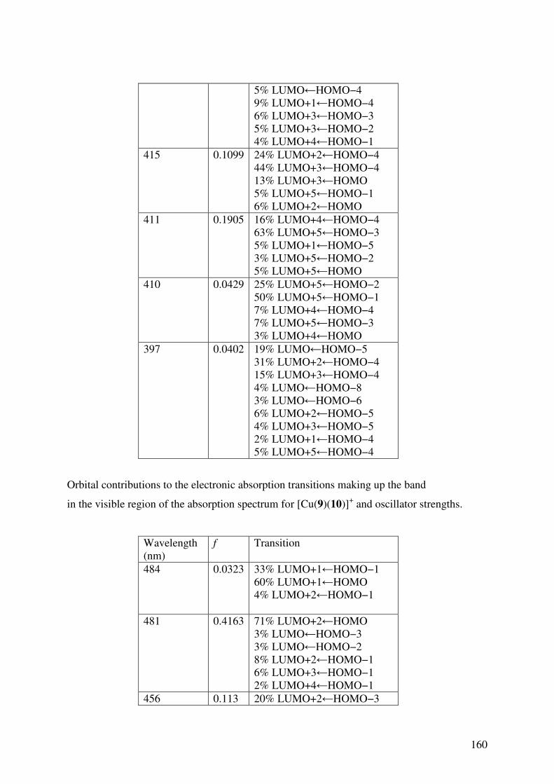
160

5% LUMO←HOMO−4 9% LUMO+1←HOMO−4 6% LUMO+3←HOMO−3 5% LUMO+3←HOMO−2 4% LUMO+4←HOMO−1

415 0.1099 24% LUMO+2←HOMO−4 44% LUMO+3←HOMO−4 13% LUMO+3←HOMO 5% LUMO+5←HOMO−1 6% LUMO+2←HOMO

411 0.1905 16% LUMO+4←HOMO−4 63% LUMO+5←HOMO−3 5% LUMO+1←HOMO−5 3% LUMO+5←HOMO−2 5% LUMO+5←HOMO

410 0.0429 25% LUMO+5←HOMO−2 50% LUMO+5←HOMO−1 7% LUMO+4←HOMO−4 7% LUMO+5←HOMO−3 3% LUMO+4←HOMO

397 0.0402 19% LUMO←HOMO−5 31% LUMO+2←HOMO−4 15% LUMO+3←HOMO−4 4% LUMO←HOMO−8 3% LUMO←HOMO−6 6% LUMO+2←HOMO−5 4% LUMO+3←HOMO−5 2% LUMO+1←HOMO−4 5% LUMO+5←HOMO−4

Orbital contributions to the electronic absorption transitions making up the band

in the visible region of the absorption spectrum for [Cu(9)(10)]+ and oscillator strengths.

Wavelength (nm)

f Transition

484 0.0323 33% LUMO+1←HOMO−1 60% LUMO+1←HOMO 4% LUMO+2←HOMO−1

481 0.4163 71% LUMO+2←HOMO 3% LUMO←HOMO−3 3% LUMO←HOMO−2 8% LUMO+2←HOMO−1 6% LUMO+3←HOMO−1 2% LUMO+4←HOMO−1

456 0.113 20% LUMO+2←HOMO−3

161

22% LUMO+2←HOMO−2 29% LUMO+2←HOMO−1 4% LUMO+1←HOMO−3 6% LUMO+1←HOMO−2 6% LUMO+1←HOMO−1 3% LUMO+3←HOMO−1 5% LUMO+2←HOMO

444 0.4481 10% LUMO+3←HOMO−2 62% LUMO+3←HOMO−1 2% LUMO+2←HOMO−1 6% LUMO+2←HOMO 6% LUMO+3←HOMO 5% LUMO+4←HOMO

440 0.044 13% LUMO←HOMO−6 37% LUMO+1←HOMO−2 12% LUMO+2←HOMO−2 13% LUMO+3←HOMO 2% LUMO+4←HOMO−2 2% LUMO+1←HOMO−1 6% LUMO+4←HOMO−1 6% LUMO+4←HOMO

439 0.0799 22% LUMO+1←HOMO−2 44% LUMO+3←HOMO 3% LUMO+3←HOMO−2 4% LUMO+4←HOMO−2 9% LUMO+4←HOMO−1 8% LUMO+4←HOMO

433 0.1185 36% LUMO←HOMO−6 15% LUMO+1←HOMO−2 15% LUMO+3←HOMO 10% LUMO+4←HOMO 7% LUMO←HOMO−4 2% LUMO+4←HOMO−2 5% LUMO+3←HOMO−1 5% LUMO+4←HOMO−1

431 0.2702 29% LUMO←HOMO−6 10% LUMO+3←HOMO−1 17% LUMO+4←HOMO−1 12% LUMO+3←HOMO 10% LUMO+4←HOMO 4% LUMO←HOMO−4 3% LUMO+2←HOMO−2 7% LUMO+4←HOMO−2

421 0.1904 40% LUMO+4←HOMO−1 39% LUMO+4←HOMO 2% LUMO+3←HOMO−2 8% LUMO+5←HOMO

417 0.1785 49% LUMO+5←HOMO−1

162

26% LUMO+5←HOMO 3% LUMO+2←HOMO−3 8% LUMO+5←HOMO−2 2% LUMO+4←HOMO−1 8% LUMO+4←HOMO

409 0.0513 17% LUMO+1←HOMO−3 41% LUMO+3←HOMO−2 7% LUMO+2←HOMO−3 8% LUMO+2←HOMO−2 3% LUMO+2←HOMO−1 4% LUMO+5←HOMO−1 6% LUMO+3←HOMO 6% LUMO+4←HOMO

406 0.0991 43% LUMO+1←HOMO−3 28% LUMO+3←HOMO−2 9% LUMO+2←HOMO−2 5% LUMO+4←HOMO−2 3% LUMO+3←HOMO−1 3% LUMO+4←HOMO−1 2% LUMO+3←HOMO

403 0.041 24% LUMO+1←HOMO−3 21% LUMO+2←HOMO−3 18% LUMO+4←HOMO−2 7% LUMO←HOMO−7 5% LUMO←HOMO−4 4% LUMO+1←HOMO−2 4% LUMO+2←HOMO−2 6% LUMO+4←HOMO−1

Orbital contributions to the electronic absorption transitions making up the band

in the visible region of the absorption spectrum for [Cu(9)(11)]+ and oscillator strengths.

Wavelength (nm)

f Transition

478 0.1443 21% LUMO+1←HOMO−3 10% LUMO←HOMO−2 14% LUMO+1←HOMO−2 30% LUMO+1←HOMO−1 9% LUMO←HOMO−3 3% LUMO+1←HOMO 7% LUMO+2←HOMO

464 0.2154 15% LUMO+1←HOMO−3 13% LUMO+1←HOMO−2 47% LUMO+1←HOMO−1 4% LUMO+2←HOMO

451 0.068 15% LUMO+1←HOMO−3

163

10% LUMO+1←HOMO−1 39% LUMO+1←HOMO 10% LUMO+2←HOMO 3% LUMO←HOMO−3 6% LUMO+1←HOMO−2 4% LUMO+2←HOMO−2 7% LUMO+2←HOMO−1

442 0.4719 20% LUMO+1←HOMO−1 17% LUMO+2←HOMO−1 38% LUMO+2←HOMO 4% LUMO←HOMO−3 2% LUMO←HOMO−2 3% LUMO+1←HOMO−2 8% LUMO+2←HOMO−2

434 0.1323 51% LUMO+2←HOMO−1 27% LUMO+2←HOMO 9% LUMO+2←HOMO−2 4% LUMO+3←HOMO−1 2% LUMO+1←HOMO

428 0.1036 11% LUMO+1←HOMO−2 12% LUMO+3←HOMO−2 42% LUMO+3←HOMO−1 5% LUMO←HOMO−6 8% LUMO←HOMO−5 2% LUMO←HOMO−4 2% LUMO+1←HOMO−1 5% LUMO+2←HOMO 6% LUMO+3←HOMO

424 0.1707 24% LUMO←HOMO−6 34% LUMO←HOMO−5 10% LUMO←HOMO−4 10% LUMO+3←HOMO−1 5% LUMO+3←HOMO−2 3% LUMO+2←HOMO 5% LUMO+3←HOMO

411 0.0363 14% LUMO+4←HOMO−2 44% LUMO+4←HOMO−1 30% LUMO+4←HOMO

410 0.2965 18% LUMO+1←HOMO−3 15% LUMO+1←HOMO−2 21% LUMO+3←HOMO−1 23% LUMO+3←HOMO 7% LUMO+2←HOMO−2 3% LUMO+2←HOMO−1

405 0.0549 23% LUMO+2←HOMO−3 32% LUMO+2←HOMO−2 12% LUMO+4←HOMO 4% LUMO+1←HOMO−3

164

4% LUMO+1←HOMO−2 2% LUMO+5←HOMO−2 7% LUMO+2←HOMO−1 6% LUMO+5←HOMO−1 3% LUMO+5←HOMO

396 0.0353 51% LUMO+2←HOMO−3 14% LUMO+2←HOMO−2 11% LUMO+3←HOMO−2 4% LUMO←HOMO−7 7% LUMO+3←HOMO−3 2% LUMO+2←HOMO−1 5% LUMO+2←HOMO−1 2% LUMO+3←HOMO

Orbital contributions to the electronic absorption transitions making up the band

in the visible region of the absorption spectrum for [Cu(9)(12)]+ and oscillator strengths.

Wavelength (nm)

f Transition

473 0.3897 11% LUMO←HOMO−3 15% LUMO+1←HOMO−3 21% LUMO+1←HOMO−1 13% LUMO+3←HOMO−1 13% LUMO+1←HOMO 6% LUMO←HOMO−2 3% LUMO+1←HOMO−2 3% LUMO+3←HOMO−2 9% LUMO+3←HOMO

468 0.2013 39% LUMO+1←HOMO−3 16% LUMO+1←HOMO−2 16% LUMO+1←HOMO−1 14% LUMO+1←HOMO 3% LUMO←HOMO−2 3% LUMO+2←HOMO 2% LUMO+4←HOMO

450 0.1386 16% LUMO+4←HOMO−2 15% LUMO+1←HOMO−1 13% LUMO+1←HOMO 16% LUMO+3←HOMO 18% LUMO+4←HOMO 6% LUMO←HOMO−3 2% LUMO←HOMO−2 7% LUMO+3←HOMO−2 3% LUMO+4←HOMO−1

444 0.1268 11% LUMO+4←HOMO−2 22% LUMO+1←HOMO

165

31% LUMO+4←HOMO 6% LUMO←HOMO−3 3% LUMO←HOMO−2 9% LUMO+1←HOMO−2 6% LUMO+1←HOMO−1 3% LUMO+4←HOMO−1

433 0.4728 73% LUMO+3←HOMO−1 10% LUMO+3←HOMO 2% LUMO←HOMO−3 3% LUMO+4←HOMO−2

422 0.0391 72% LUMO+2←HOMO−2 4% LUMO+3←HOMO−2 4% LUMO+2←HOMO 5% LUMO+3←HOMO 4% LUMO+5←HOMO

416 0.0912 34% LUMO+3←HOMO−2 13% LUMO+3←HOMO 23% LUMO+5←HOMO 2% LUMO+1←HOMO−3 8% LUMO+3←HOMO−3 3% LUMO+1←HOMO−2 4% LUMO+5←HOMO−2 4% LUMO+4←HOMO−1

415 0.5465 55% LUMO+4←HOMO−1 22% LUMO+4←HOMO 8% LUMO+1←HOMO−3 7% LUMO+1←HOMO−2

404 0.0641 29% LUMO+4←HOMO−2 13% LUMO+5←HOMO−1 10% LUMO+4←HOMO 12% LUMO+5←HOMO 7% LUMO←HOMO−5 3% LUMO←HOMO−4 2% LUMO+1←HOMO−3 8% LUMO+3←HOMO−3 5% LUMO+4←HOMO−3 2% LUMO+4←HOMO−1

391 0.0327 88% LUMO+2←HOMO−3 5% LUMO+3←HOMO−3 3% LUMO+7←HOMO−3

166

Chapter 6

Copper(I) complexes with pendant pyridyl functionalities for application in DSSCs

6.1 Introduction

The necessary properties of copper(I) complexes for use in dye-sensitised solar cells have

been described in chapter 4. One important requirement of the complex is that it absorbs

over a large portion of the visible spectrum. Complexation of one or more quaterpyridine

ligands, 4,4':2',2'':4'',4'''-quaterpyridine (Fig. 6.1) to ruthenium has been reported to red-

shift the absorption spectrum of the complex compared to that of [Ru(bpy)3]2+ 1-3

.

Fig. 6.1 4,4':2',2'':4'',4'''-Quaterpyridine.

As it is, this ligand is unsuitable for complexation to copper(I) atoms. To eliminate the

possibility of auto-oxidation of the copper(I) atom it is necessary to incorporate blocking

groups, typically methyl substituents, at the sites adjacent to the N,N' metal binding sites

of the bipyridine unit. Synthesis of this 6',6''-dimethyl-4,4':2',2'':4'',4'''-quaterpyridine

ligand has previously been attempted by members of the Constable group and has been

unsuccessful. Consequently, another ligand with four pyridine groups and substitutions in

the 6,6'-positions of the 2,2'-bipyridine unit was developed.

Coe et al. reported the use of a ligand with four pyridine groups and substitution in the

4- and 4'-positions of the 2,2'-bipyridine unit (Fig. 6.2)4. However, this ligand was still

unsubstituted in the 6- and 6'-positions.

Fig. 6.2 4,4'-Bis((E)-2-(pyridin-4-yl)vinyl)-2,2'-bipyridine reported by Coe et al in 20104.

167

Therefore, the initial aim of this chapter was to synthesise 6,6'-bis((E)-2-(pyridin-4-

yl)vinyl)-2,2'-bipyridine. The use of this ligand has been previously reported by

Shonfield et al. in 19995 but details of the synthesis were not published. For that reason, a

number of synthetic routes to obtain this compound were attempted and are detailed in

Fig. 6.3.

N

N

N

N N

N

OH

N

N

N

N N

N

OH

N

N

N

N N

N

OH

KOtBu, DMF

Argon, Dark

Toluene

150OC, 11 hr, W

NaH, THF,

Argon, -70oC to 25oC

N

N

N

Fig. 6.3 Failed synthetic procedures to the quaterpyridine ligand.

All of the synthetic approaches detailed in Fig. 6.3 failed and so a stepwise procedure of

first synthesising the 2,2'-([2,2'-bipyridine]-6,6'-diyl)bis(1-(pyridin-4-yl)ethanol) and then

dehydrating it to form the alkene was adopted (Scheme 6.1).

N

N

N

N N

N

OH

LDA, THF,

N2, -70oC to 25oC

HO

N

OH

N

N

N

N

AcOH

Reflux

Scheme 6.1 Proposed synthetic route to 6,6'-bis((E)-2-(pyridin-4-yl)vinyl)-2,2'-bipyridine.

168

The stepwise procedure failed; regardless of the number of equivalents of 4-pyridine

carbaldehyde and lithium diisopropylamide (LDA) added to the reaction, it was only

possible to form the mono-substituted compound, 2-(6'-methyl-[2,2'-bipyridin]-6-yl)-1-

(pyridin-4-yl)ethanol (14). The product of this reaction was then dehydrated to form the

mono-substituted compound (E)-6-methyl-6'-(2-(pyridine-4-yl)vinyl)-2,2'-bipyridine (15).

The ligands depicted in Fig 6.4, and complexes thereof, are described in this chapter.

Fig. 6.4 Ligands 14 and 15 with labelling for spectroscopic assignments.

6.2 Synthesis - Ligands

The starting material for 14 was 6,6'-dimethyl-2,2'-bipyridine (8), which was

commercially available. Compound 14 was synthesised in a stepwise manner (Scheme

6.2) by first deprotonating 8 using LDA in dry THF at -78°C. Then 1.3 equivalents of

pyridine-4-carbaldehyde were added and the reaction was left to warm to room

temperature, whilst stirring, overnight. The compound was extracted into

dichloromethane and purified using column chromatography. The yield of the reaction

was 65%.

Scheme 6.2 The synthesis of compound 14.

A by-product formed during the reaction and was identified, using 1H NMR spectroscopy

and X-ray crystallography, as pyridin-4-yl isonicotinate (16), a compound related to the

4-pyridine carbaldehyde starting material (Fig. 6.5).

169

Fig. 6.5 Compound 16, the by-product formed during the synthesis of 14.

Compound 15 was synthesised by refluxing 14 in acetic acid overnight (Scheme 6.3).

Scheme 6.3 The synthesis of compound 15.

The compound was then neutralised with sodium hydrogencarbonate (NaHCO3) and

extracted with dichloromethane and purified by column chromatography. By carrying out

a very slow column and collecting very small fractions it was possible to isolate a small

amount of pure 15 from the early fractions. In the later fractions, 15 is contaminated by

the related enol compound, 17 (Fig. 6.6), which is formed as a by-product in the reaction.

This compound has almost the same Rf value as 15 regardless of the solvent system and

the compounds 15 and 17 even co-crystallise.

Fig. 6.6 Compound 17 in the keto- and enol-tautomeric forms.

Initially it was thought that the formation of the enol was due to the presence of oxygen

in the reaction. However, repeating the reaction under Schlenk conditions gave the same

products, 15 and 17, in the same yield.

170

6.3 Results and Discussion (I)

6.3.1 1

H NMR Spectroscopy - Ligands

The 1H NMR spectrum of compound 14 was measured in CDCl3 and the spectrum is

depicted in Fig. 6.7.

Fig. 6.7 1H NMR spectrum of 14 (500 MHz, CDCl3, 25ºC, TMS) CHCl3 (*),

Ethylacetate (ǂ).

The 1H NMR spectrum of 14 (Fig. 6.7) was assigned using both COSY and NOESY

techniques. The singlet at δ 2.64 ppm was ascribed to the methyl substituent due to the

chemical shift and the integral. The two signals with integrals of two were assigned to the

C ring and the specific assignment of the peaks was done using a NOESY spectrum. The

signal at δ 8.57 ppm showed no NOESY cross peaks and was therefore assigned as C2.

The signal at δ 7.36 ppm showed a NOESY cross peak to the doublet of doublets at

C2

B3 A3

B4 A4 C3

A5 B5

d

c

b

*

ǂ

a

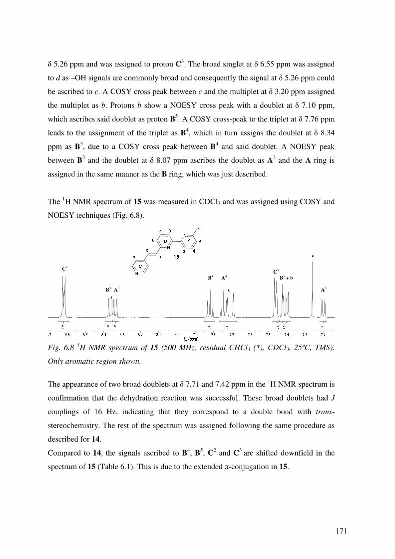
171

δ 5.26 ppm and was assigned to proton C3. The broad singlet at δ 6.55 ppm was assigned

to d as –OH signals are commonly broad and consequently the signal at δ 5.26 ppm could

be ascribed to c. A COSY cross peak between c and the multiplet at δ 3.20 ppm assigned

the multiplet as b. Protons b show a NOESY cross peak with a doublet at δ 7.10 ppm,

which ascribes said doublet as proton B5. A COSY cross-peak to the triplet at δ 7.76 ppm

leads to the assignment of the triplet as B4, which in turn assigns the doublet at δ 8.34

ppm as B3, due to a COSY cross peak between B

4 and said doublet. A NOESY peak

between B3 and the doublet at δ 8.07 ppm ascribes the doublet as A

3 and the A ring is

assigned in the same manner as the B ring, which was just described.

The 1H NMR spectrum of 15 was measured in CDCl3 and was assigned using COSY and

NOESY techniques (Fig. 6.8).

Fig. 6.8 1H NMR spectrum of 15 (500 MHz, residual CHCl3 (*), CDCl3, 25ºC, TMS).

Only aromatic region shown.

The appearance of two broad doublets at δ 7.71 and 7.42 ppm in the 1H NMR spectrum is

confirmation that the dehydration reaction was successful. These broad doublets had J

couplings of 16 Hz, indicating that they correspond to a double bond with trans-

stereochemistry. The rest of the spectrum was assigned following the same procedure as

described for 14.

Compared to 14, the signals ascribed to B4, B

5, C

2 and C

3 are shifted downfield in the

spectrum of 15 (Table 6.1). This is due to the extended π-conjugation in 15.

C2

*

B3 A3

B4 A4

c

C3 B5 + b

A5

172

Compound B4 B

5 C

2 C

3

14 7.76 7.10 8.57 7.36

15 7.83 7.42 8.62 7.47

Table 6.1 Comparison of shifts (δ/ppm) for compounds 14 and 15. Spectra measured in

CDCl3 at room temperature.

6.3.2 13

C1H NMR Spectroscopy - Ligands

The 13

C1H NMR spectrum of 14 was measured in CDCl3 and is depicted in Fig 6.9.

Fig. 6.9 13C1H NMR spectrum of 14 (126 MHz, CDCl3, 25ºC, TMS).

The spectrum was ascribed using HMQC and HMBC techniques along with a DEPT 135

spectrum (Fig. 6.10). The assignment of b was facile as –CH2- groups “point down” in

DEPT 135 spectra.

Fig. 6.10 DEPT135 spectrum of 14 specifically showing the signal ascribed to b.

A6 + B6 B2 A2 C4

C2

B4 A4

A5 + B5

C3

A3 B3

c

b

a

173

The peaks arising from 13

C-H carbons were assigned using the HMQC spectrum and the

quaternary carbon signals were assigned using the HMBC spectrum. Proton C2 had an

HMBC interaction with a signal at δ 152.9 ppm, which was assigned to C4

(Fig. 6.11). An

HMBC interaction between proton c and a signal at δ 158.3 ppm meant that said signal

could be ascribed to B6. Proton B

4 had two HMBC interactions; one to the peak at δ 158.3

ppm, already ascribed to B6, and one to a peak at δ 155.7, ascribing the latter peak to B

2.

The assignment of the peak at δ 155.7 ppm was confirmed on observation of a HMBC

interaction between proton A3 and the signal ascribed to B

2. The carbon signal for A

2 was

assigned after observation of a HMBC interaction from B3 to a signal at δ 154.8 ppm.

Proton A4 showed two HMBC interactions, the first to the signal at δ 154.8 ppm,

confirming the assignment as A2 and the second to a signal at δ 158.4 ppm, assigning this

latter signal to A6

(Fig. 6.11).

Fig 6.11 HMBC spectrum of compound 14, measured in CDCl3 at 25ºC, depicting the

interactions between H(A4) and C(A2), C(A6) and H(C3) and C(C4) specifically.

The 13

C1H spectrum of 15 was also measured in CDCl3 and the spectrum was assigned

using HMQC and HMBC techniques. The cross peaks between the alkene protons and

their respective carbon signals were very distinct (Fig. 6.12). All carbons except the

C3 B4 A4

A3 B3

C4

A2

A6

174

quaternary carbons were assigned using the HMQC spectrum. The quaternary carbons

were assigned using the HMBC spectrum in the manner previously described for 14.

Fig. 6.12 Partial HMQC spectrum of 15, measured in CDCl3 at 25ºC.

6.3.3 Mass Spectrometry – Ligands

Compounds 14 and 15 were characterised using ESI mass spectrometry. For 14, a peak

corresponding to [M+Na]+

was observed at m/z 314.2 which was in good agreement with

the calculated peak (314.1) and therefore confirmed that the synthesis of the compound

had been successful.

Two peaks were observed in the ESI mass spectrum of 15. These peaks corresponded to

[M+K]+ and [M+Na]

+ at m/z 312.1 and 296.2 respectively. Again the experimentally

observed values were in good agreement with the calculated values and confirmed that

the dehydration of the alcohol to form the alkene had been successful.

c b

b

c

175

6.3.4 Absorption Spectroscopy - Ligands

0

5000

10000

15000

20000

25000

240 260 280 300 320 340 360 380

Wavelength (nm)

ε (

dm

3 m

ol-1

cm

-1)

14

15

Fig. 6.13 Absorption spectra for 14 and 15 measured in dichloromethane (10-5 mol dm-3).

The electronic absorption spectra are dominated by ligand-based π→π* transitions and

the data are summarised in Table 6.2.

Table 6.2 A summary of the photophysical data, recorded in dichloromethane, for 14 and

15.

The absorptions at 247, 283, 293 and 303 nm of compound 14 are all due to the

bipyridine unit6. This is unsurprising as there is no conjugation between the bipyridine

moiety and the pendant pyridyl unit. No absorption due to the pendant pyridyl unit is

observed in the spectrum.

The absorption spectrum of 15 is very different. Contribution to the spectrum from the

bipyridine unit is observed in the high energy region of the spectrum, namely the peak

with λmax = 285 nm. The lower energy peaks are a result of the conjugation between the

pendant pyridyl ring and the bipyridine unit through the double bond.

Compound

14 303

(16262)

293

(24883)

283 sh

(20261)

247

(15440)

15 342 sh

(7215)

327

(11612)

285

(18186)

λmax

(ε, dm3 mol

-1 cm

-1)

176

6.3.5 Emission and Excitation Spectroscopy - Ligands

0

0.2

0.4

0.6

0.8

1

300 350 400 450 500 550 600

Wavelength (nm)

Inte

nsit

y (

a.u

.)

emission (ex 293 nm)

emission (ex 306 nm)

Fig. 6.14 Emission spectra of 14 measured in dichloromethane.

The origins of the emissions at 329, 342 and 359 nm were confirmed by measuring

excitation spectra. The emission centred at 480 nm could be due to the formation of an

exciplex. The excitation spectrum, when holding the emission at 480 nm, is dissimilar to

the absorption spectrum (Fig. 6.15).

0

1

250 300 350 400 450

Wavelength (nm)

Inte

nsit

y (

a.u

.)

excitation (em 470 nm)

Fig. 6.15 Excitation spectrum of 14 measured in dichloromethane.

The dissimilarity between the absorption and excitation spectra indicates that the origin

of the emission is through a non-luminescent absorption. Further investigation by testing

the effect of a more polar solvent, such as methanol, on the exciplex needs to be carried

out.

177

0

1

350 375 400 425 450 475

Wavelength (nm)

Inte

nsit

y (

a.u

.) emission (ex 285 nm)

emission (ex 328 nm)

Fig. 6.16 Emission spectra of 15 measured in dichloromethane.

The emission spectrum of 15 is red-shifted compared to that of 14 due to the extended π-

conjugation. The origins of the emissions at 358, 374 and 394 nm were confirmed by

measuring excitation spectra.

6.3.6 Crystal Structures - Ligands

Single colourless needles of 14 were grown by diffusion of hexanes into a

dichloromethane solution of the complex. The crystal solves in the monoclinic P21/c

space group with a reasonable R factor of 7.8%. The asymmetric unit contains one

molecule of 14. The structure of the molecule is depicted in Fig. 6.17 and selected bond

lengths and angles are listed in the caption.

178

Fig. 6.17 Structure of 14 with ellipsoids plotted at 50% probability and hydrogen atoms

omitted for clarity. Selected bond parameters: N1-C2 = 1.344(5), N1-C6 = 1.342(5),

N2-C7 = 1.353(5), N2-C11 = 1.341(5), N3-C14 = 1.345(5), N3-C18 = 1.330(6),

C11-C12 = 1.509(6), C12-C13 = 1.550(5), C13-O1 = 1.407(5), C13-C16 = 1.497(6) Å;

N1-C2-C1 = 116.1(3), N2-C11-C12 = 118.0(3), C11-C12-C13 = 112.9(3),

C12-C13-C16 = 109.2(3), C14-N3-C18 = 116.2(4)°.

As expected, the bipyridine unit is in the trans-conformation. The bond lengths around

the bipyridine and pyridine units are unexceptional. The C11-C12 and C13-C16 bonds

are the same length, within experimental error, and the lengths are consistent with single

bonds. By comparison, the C12-C13 bond is elongated slightly but still consistent with a

single bond. As expected the C13-O1 bond is longer than the single C-C bonds and

shorter than the ring C-C bonds. The molecule is not planar and the rings containing

atoms N1 and N2 are essentially coplanar. The molecules pack in chains due to hydrogen

bonds between the –OH group (H1) on one molecule and the nitrogen atom (N3) of the

pendant pyridyl ring on another molecule and both enantiomers can be observed in the

packing (Fig. 6.18).

N1

C2

C1

C6 C7

N2

C11

C12

O1

N3

C13

C16

C14

C18

179

Fig. 6.18 Packing of 14 with the hydrogen bonds between the molecules denoted by

dashed blue lines.

Colourless blocks of 15 were grown following the same procedure for 14. The crystal

solved in the monoclinic C2/c space group with a good R factor of 3.6%. The asymmetric

unit contains one molecule of 15 and there is no solvent present in the crystal lattice. The

structure of 15 is depicted in Fig. 6.19 and selected bond lengths and angles are listed in

the caption.

Fig. 6.19 Structure of 15 with ellipsoids plotted at 50% probability and hydrogen atoms

omitted for clarity. Selected bond parameters: C11-C12 = 1.467(1), C12-C13 = 1.334(1),

C13-C16 = 1.467(1) Å; N1-C2-C1 = 116.32(9), N2-C11-C12 = 114.89(9),

C11-C12-C13 =126.77(9), C12-C13-C16 = 124.17(9)°.

As for 14 the bipyridine unit is in the trans-conformation. The main differences between

the structures of 14 and 15 are the absence of the alcohol group in the structure of 15 and

the shortening of the C12-C13 bond. Both of these differences are confirmation that the

dehydration of the alcohol to form the alkene was successful. All other bond lengths are

unremarkable.

N1

N2

N3

C11

C12

C13

C16

C2

C1

180

The packing of the molecules is determined by hydrogen bonds between the proton on

one pendant pyridyl moiety (H18) and the nitrogen atom of another pendant pyridyl

moiety (N3). This is depicted in Fig. 6.20.

Fig. 6.20 Packing of 15 with the hydrogen bonds between the molecules denoted by

dashed red lines.

As stated in Section 6.2, ligand 15 co-crystallises with the reaction by-product,

compound 17. This is depicted in Fig. 6.21. Yellow blocks were grown through slow

evaporation of an ethylacetate and hexane solution. The crystal solves in the monoclinic

P21/c space group with a good R factor of 3.8%. Ligand 15 is predominantly present in

the crystal, with 17 present a third of the time. Compound 17 is present as the enol form

of the keto-enol tautomer and there is an internal hydrogen bond between the bipyridine

nitrogen and the proton of the enol moiety (denoted by the dashed blue line in Figs. 6.22)

Fig. 6.21 The structure in the asymmetric unit of the co-crystallised compounds 15 and

17. Ellipsoids plotted at 50% probability.

H of alkene

OH of enol

181

Fig. 6.22 (Left) The desired compound, 15. (Right) The reaction by-product, 17.

Ellipsoids plotted at 50% probability in both cases.

The molecules pack with a mixture of face-to-face and edge-to-face interactions between

the pyridine rings (Fig. 6.23). Contrary to the structures of 14 and 15 there is no

hydrogen-bonding utilising the pendant pyridine nitrogen.

Fig. 6.23 Packing of the structure of co-crystallised 15 and 17 with the short contacts

denoting edge-to-face and face-to-face interactions with dashed red lines.

Compound 16 was another by-product, formed during the reaction of 8 with 4-pyridine

carbaldehyde. Colourless needles were grown by evaporation of ethyl acetate and hexane

from a solution of the compound. The crystal solved in the monoclinic P21/c space group

with a reasonable R factor of 6.26 %. The asymmetric unit contained one molecule of 16

and it is depicted in Fig. 6.24. As the compound was a reaction by-product there is no

detailed discussion following the picture of the structure.

182

Fig. 6.24. Structure of 16 with ellipsoids plotted at 50% probability and hydrogens

omitted for clarity.

6.4 Synthesis - Cu(I) Complexes

The Cu(I) complexes were synthesised by addition of two equivalents of the relevant

ligand, in chloroform, to one equivalent of [Cu(NCMe)4][PF6], in acetonitrile. The

complexes were isolated as red powders in good yield.

Scheme 6.3 Synthesis of [Cu(14)2][PF6], yield = 70 %.

Scheme 6.4 Synthesis of [Cu(15)2][PF6], yield = 85 %.

6.5 Results and Discussion (II)

6.5.1 Section Introduction

Chiral copper(I) complexes arise from the coordination of two asymmetric ligands to a

copper(I) atom and were first reported by Thummel et al. in 20017. As Cu(I) is labile, the

183

ligands exchange in solution and so variable temperature NMR was used to investigate

the rates of ligand exchange in acetonitrile and chloroform. Sauvage et al. also reported

chiral Cu(I) complexes in 20068. Variable temperature NMR and introduction of an

enantiopure chiral anion to the complexes were used to ascertain the stereoisomers

present in solution and the stability of those isomers. The chirality of the copper(I) is

denoted ∆ or Λ9.

6.5.2 1H NMR Spectroscopy – Cu(I) Complexes

The 1H NMR spectrum of [Cu(15)2][PF6] was measured at room temperature and the

signals were found to be broad, which lead to the hypothesis that the pendant pyridine

group (ring C) was rotating in a hindered fashion on the NMR timescale. Therefore,

variable temperature NMR spectroscopy was used to investigate the effect of temperature

on the rotation of the C ring (Fig. 6.25).

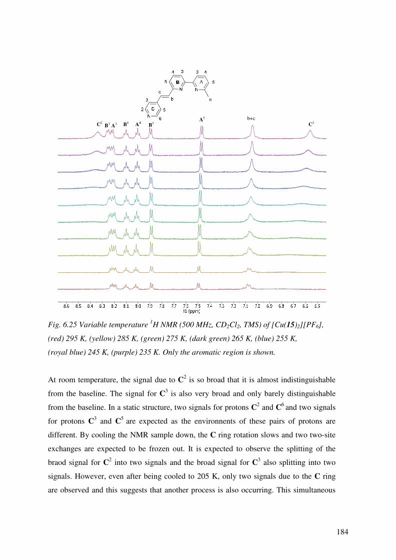
184

Fig. 6.25 Variable temperature 1H NMR (500 MHz, CD2Cl2, TMS) of [Cu(15)2][PF6],

(red) 295 K, (yellow) 285 K, (green) 275 K, (dark green) 265 K, (blue) 255 K,

(royal blue) 245 K, (purple) 235 K. Only the aromatic region is shown.

At room temperature, the signal due to C2 is so broad that it is almost indistinguishable

from the baseline. The signal for C3 is also very broad and only barely distinguishable

from the baseline. In a static structure, two signals for protons C2 and C

6 and two signals

for protons C3 and C

5 are expected as the environnents of these pairs of protons are

different. By cooling the NMR sample down, the C ring rotation slows and two two-site

exchanges are expected to be frozen out. It is expected to observe the splitting of the

braod signal for C2 into two signals and the broad signal for C

3 also splitting into two

signals. However, even after being cooled to 205 K, only two signals due to the C ring

are observed and this suggests that another process is also occurring. This simultaneous

C2 C3

b+c

B4 A4 B3 A3 B5 A5

185

process is probably due to the interconversion of enantiomers10

. The signal due to the

methyl groups does not change throughout the cooling process.

The 1H NMR spectrum was assigned by means of a COSY spectrum, which was

measured at 205 K, and by comparison of the 1H NMR spectrum of the ligand with the

1H NMR spectrum of the complex.

The 1H NMR spectrum of [Cu(14)2][PF6] was more complicated than that of

[Cu(15)2][PF6] due to the presence of an asymmetric carbon atom in each ligand,

resulting in diastereoisomers and enantiomers of the complex (Fig. 6.25). The

asymmetric chiral carbon atoms in the following structures are assigned according to the

rule set out by Cahn, Ingold and Prelog11

and as such, are denoted R or S. Due to the

asymmetric ligand and the chiral centres in [Cu(14)2][PF6], the product of the reaction

consisted of six possible complexes; a mix of diastereoisomers and enantiomers (Fig.

6.26).

Fig. 6.26 The combinations of enantiomers and diastereoisomers possible for [Cu(14)2]+.

186

The compounds ∆-R,R and Λ-S,S are enantiomers and so only one signal due to each

proton environment for both of these compounds was expected in the NMR. The same is

true for compounds ∆-S,S and Λ-R,R. ∆-R,S is an enantiomer of Λ-S,R and ∆-S,R is an

enantiomer Λ-R,S. The compounds ∆-R,S and ∆-S,R are chemically equivalent, as are

Λ-S,R and Λ-R,S. The four pairs of enantiomers (∆-R,R+Λ-S,S and ∆-S,S+Λ-R,R and ∆-

R,S+Λ-S,R and Λ-R,S+ ∆-S,R) are diastereoisomers of one another. Assuming that the

signals for ∆-R,S+Λ-S,R and Λ-R,S+ ∆-S,R are coincident, then three sets of signals

should be observed in the 1H NMR spectrum of [Cu(14)2][PF6].

At room temperature the spectrum of the complex is broad, consequently variable

temperature NMR was used to try to observe the separation of diastereoisomers on

cooling (Fig. 6.27).

Fig. 6.27 Variable temperature 1H NMR (500 MHz, CD3CN, TMS) of [Cu(15)2][PF6],

(red) 298 K, (yellow) 295 K, (green) 283 K, (light blue) 273 K, (royal blue) 263 K,

(purple) 253 K. Only the aromatic region is shown.

On cooling, the broad peaks observed at room temperature begin to split and the very

broad signal at δ 6.70 ppm becomes sharper.

187

The presence of diastereoisomers is more easily identifiable in the aliphatic region of the

spectrum, specifically the CH(OH) and methyl signals (Fig. 6.28). The –CH2– signal (b)

changes very little on cooling and is therefore not shown.

Fig. 6.28 Variable temperature 1H NMR (500 MHz, CD3CN, TMS) of [Cu(15)2][PF6],

(red) 298 K, (yellow) 295 K, (green) 283 K, (light blue) 273 K, (royal blue) 263 K,

(purple) 253 K. Only the aliphatic region is shown.

On cooling it is possible to observe the broad signal at δ 4.71 separating into two signals

and the broad signal at δ 2.89 ppm becomes at least three signals. Contrary to the methyl

signal of [Cu(15)2][PF6], which does not change on cooling, the methyl signal of

[Cu(14)2][PF6] appears to split. Overall, the signals remain broad at 253 K, and lower

temperature spectra need to be recorded if this investigation is to be expanded. It has not

yet been possible to fully elucidate the processes that involve the interconversion of

diastereoisomers and the interconversion of enantiomers (ie. the same process as in

[Cu(15)2][PF6] 10

).

Methyl signals CH(OH) signals

188

Future work should include further investigation of the NMR spectra by changing the

solvent to deuterated dichloromethane and cooling the sample further.

The enantiomerically pure NMR solvating agent ∆-TRISPHAT was added, as

[NBu4][ ∆-TRISPHAT], to the NMR sample of [Cu(14)2][PF6] to separate out the

enantiomers by making them diastereoisomers, which are individually distinguishable in

the NMR spectrum as, for example, [∆-R,R-Cu(14)2]+[∆-X]

- is chemically different to

[Λ-R,R-Cu(14)2]+[∆-X]

-. Six sets of signals were then expected in the

1H NMR spectrum.

Fig. 6.29 Bottom, 1H NMR spectrum of [Cu(14)2][PF6] with added ∆-TRISPHAT

(400 MHz, CD3CN, TMS,25°C), Top , 1H NMR spectrum of [Cu(14)2][PF6] without ∆-

TRISPHAT (500 MHz, CD3CN, TMS, 25°C).

On addition of the ∆-TRISPHAT the broad signal at δ 8.54 ppm in the spectrum with no

added ∆-TRISPHAT is shifted upfield to δ 8.35 ppm, where it overlaps with the doublet

of doublets at δ 8.25 ppm. The broad signal at δ 8.05 ppm is split into a multiplet on

C2

d

c

189

addition of the ∆-TRISPHAT and the signal at δ 7.52 ppm becomes a well defined

doublet. The signals due to the aliphatic protons at δ 6.60, 4.72, 3.56 and 2.89 ppm also

become sharper on addition of the ∆-TRISPHAT. However, no significant changes are

observed on addition of the ∆-TRISPHAT, which is consistent with previously reported

copper(I) complexes at room temperature12

.

6.5.3 Mass Spectrometry

Both Cu(I) complexes were characterised using ESI-MS and the main peak in the

spectrum was due to [M-PF6]+. Initially both complexes were measured in acetonitrile but

in this solvent the [M-PF6]+ peak was not observed for [Cu(15)2][PF6]. On changing the

solvent to a mixture of dichloromethane and methanol it was possible to observe the

[M-PF6]+ peak at m/z 609.2. A base peak at m/z 274.1, which was assigned to protonated

ligand [15+H]+, was also observed.

6.5.4 Absorption Spectroscopy

0

5000

10000

15000

20000

25000

250 300 350 400 450 500

Wavelength (nm)

ε (

dm

3 m

ol-1

cm

-1)

14

[Cu(14)2][PF6]

Fig. 6.30 The absorption spectra of ligand 14 (measured in dichloromethane at 10-5 mol

dm-3) and its corresponding Cu(I) complex (measured in acetonitrile at 10-5 mol dm-3).

Compared to the absorption spectrum of the ligand, a new peak, centred at 450 nm, is

observed in the spectrum of [Cu(14)2][PF6] (Fig. 6.30). This is an MLCT band, which

gives rise to the orange-red colour of the complex. The high energy region of the

spectrum is very similar for both the ligand and the complex. A small amount of red-

190

shifting is observed for the high energy absorptions of the complex but this could be

attributed to the change in solvent.

0

0.2

0.4

0.6

0.8

1

250 300 350 400 450 500 550

Wavelength (nm)

Ab

so

rban

ce (

a.u

.)

15

[Cu(15)2][PF6]

Fig. 6.31 The absorption spectra of ligand 15 (measured in dichloromethane) and its

corresponding Cu(I) complex (measured in acetonitrile).

Due to the incomplete characterisation of [Cu(15)2][PF6] the concentration of the solution

could not be accurately established. For this reason, the ligand and complex absorption

spectra have been normalised for comparison (Fig. 6.31).

It was thought that coordination of a ligand with extended π-conjugation would affect the

MLCT band of the complex, however, the MLCT λmax of of both [Cu(14)2][PF6] and

[Cu(15)2][PF6] are at 450 nm. The extended π-conjugation from [Cu(14)2][PF6] to

[Cu(15)2][PF6] does affect the high energy absorptions as [Cu(15)2][PF6] absorbs a

broader range of UV light compared to [Cu(14)2][PF6].

Table 6.3 A summary of the absorption data, recorded in dichloromethane, for

[Cu(L)2][PF6] ( L = 14, 15)

Compound MLCT

λmax

(ε, 103 dm

3 mol

-1 cm

-1)

[Cu(14)2][PF6] 450

(1.9)

312 sh

(16.8)

301

(26.1)

295

(25.7)

265 sh

(20.1)

[Cu(15)2][PF6] 450 326

318 284

λmax

(ε, 103 dm

3 mol

-1 cm

-1)

191

6.5.5 Emission Data

Excitation into the MLCT band of [Cu(14)2][PF6] gave rise to an emission at 521 nm.

This emission had a lifetime of 4.6 ns, which is almost the same as the lifetime of the

related [Cu(8)2][PF6] complex (4.0 ns).

Due to the possibility of impurities in the [Cu(15)2][PF6] complex, emission and

excitation spectra were not measured.

6.5.6 Crystal Structures - Complexes

Red plates of [Cu(15)2][PF6] were grown by evaporation of a dichloromethane-methanol

solution of the complex. The crystal solved in the triclinic P-1 space group with a

reasonable R factor of 7.69%. The asymmetric unit contains one cation, two half

hexafluoridophosphate counter-anions and three water molecules. The cation is depicted

in Fig. 6.32.

Fig. 6.32 The cation [Cu(15)2]+ with ellipsoids plotted at 50% probability and hydrogens

omitted for clarity. Selected bond parameters: Cu1-N1 = 2.017(3), Cu1-N2 =2.045(4),

Cu1-N4 =2.002(3), Cu1-N5 =2.039(4), C12-C13 = 1.338(5), C30-C31 = 1.345(6) Å;

N1-Cu1-N2 = 80.7(1), N1-Cu1-N5 = 121.0(1), N2-Cu1-N4 = 115.6(1),

N4-Cu1-N5 = 81.2(1)°.

As expected, the ligand coordinates to the metal through the bipyridine nitrogen donor

atoms. The bond lengths and angles are as expected. The geometry of the complex is

N1 N2

N3

N4 N5

N6

C12

C13 C30

C31 Cu1

192

neither square planar nor tetrahedral with the angle between the two bipyridine planes

being 70.09°.

The lengths of the alkene bonds C12-C13 and C30-C31 are both the same as each other

(within experimental error) and the same as the length of the alkene bond in the crystal

structure of the ligand. Of note are the intramolecular face-to-edge and face-to-face

interactions in the cation (Fig. 6.33).

Fig. 6.33 (Left) Intramolecular face-to-edge interaction between H35A and the bipyridine

ring containing N1, (Right) Intramolecular face-to-face interaction between the pendant

pyridyl ring containing N3 and the bipyridine ring containing N4.

The packing also consists of multiple face-to-edge and face-to-face interactions between

the chains of the cations (Fig. 6.34). Contrary to the packing of the ligand there is no

intercation hydrogen bonding network through the pendant pyridyl nitrogens. This is

because it is hydrogen bonding with water molecules present in the lattice instead. The

water molecules surround the pendant pyridine sites preventing chains from forming

along the c axis (Fig. 6.35).

Both enantiomers are present in the structure and are related to one another by an

inversion centre (marked by a blue dot in Fig. 6.35).

193

Fig. 6.34 Packing of the [Cu(15)2]+ cations with interactions between the cations denoted

by dashed blue lines. Hydrogen bonding between the pendant pyridyl nitrogens and

water also shown.

Fig. 6.35 The two enantiomers of the [Cu(15)2]+ cation with water molecules blocking

the pendant pyridine sites. Hydrogens are omitted for clarity and the blue dot marks the

centre of inversion.

194

6.6 Conclusions

Two chiral copper(I) complexes have been synthesised as racemates and characterised

using a variety of techniques. Further investigation into the photophysical properties of

[Cu(15)2][PF6] and the electrochemical properties of both [Cu(14)2][PF6] and

[Cu(15)2][PF6] is necessary to decide whether the complexes are suitable for application

in dye sensitised solar cells. If this is the case then a higher-yielding synthesis of the

ligand should also be developed to enable a more efficient and cost-effective overall

synthesis of both complexes.

195

6.7 Experimental

14

Synthesis:

Under nitrogen, 8 (300 mg, 1.63 mmol) was dissolved in dry THF (30 cm3) and cooled to

-78 °C. LDA (1.2 equivalents) was added, upon which the solution turned from

colourless to black. The solution was left to stir for 30 minutes after which pyridine-4-

carbaldehyde (0.18 cm3, 1.2 eq., 1.95 mmol) was added. The solution turned from black

to golden yellow. The reaction mixture was left to stir for 12 hours, during which time it

warmed to room temperature. The reaction was then quenched with water

(10 cm3) and extracted three times with DCM (3 x 15 cm

3). The solvent was removed in

vacuo, which resulted in a brown oil. The oil was purified by chromatography (SiO2,

ethyl acetate: hexane: triethylamine, 48:33:2).

Yield: 64.5 %

1H NMR: (500 MHz, CDCl3, 25 ºC, TMS) δ/ppm: 8.57 (2H, dd, J = 6.1, 2.9 Hz, C

2),

8.34 (1H, d, J = 7.9 Hz, B3), 8.07 (1H, d, J = 7.8 Hz, A

3), 7.76 (1H, t, J = 7.4 Hz, B

4),

7.72 (1H, t, J = 7.4 Hz, A4), 7.36 (2H, dd, J = 4.5, 1.5 Hz, C

3),

7.21 (1H, d, J = 7.6 Hz, A5), 7.10 (1H, d, J = 7.6 Hz, B

5), 6.55 (1H, br s, H

d),

5.26 (1H, dd, J = 8.6, 2.9 Hz, Hc), 3.20 (2H, m, H

b), 2.64 (3H, s, H

a);

13C NMR (126 MHz, CDCl3, 25 ºC, TMS) δ/ppm: 158.4 (A

6), 158.3 (B

6), 155.7 (B

2),

154.8 (A2), 152.9 (C

1), 150.0 (C

2), 138.3 (B

4), 137.4 (A

4), 123.8 (B

5+A

5), 121.0 (C

3),

119.8 (B3), 118.0 (A

3), 72.1 (c), 44.4 (b), 24.8 (a);

ESI-MS: m/z 314.2 [M+Na]+ (calc. 314.13)

Found: C, 73.92; H, 6.15; N, 13.99; C18H17N3O requires C, 74.20; H, 5.88; N, 14.42;

Melting Point: 116.4 °C

IR (solid, υ/cm-1

): 551 (m), 579 (m), 611 (m), 615 (m), 624 (m), 632 (s), 652 (m),

663 (m), 744 (m), 750 (m), 789 (s), 807 (s), 826 (m), 976 (w), 999 (m), 1028 (w),

1035 (w), 1060 (s), 1082 (m), 1093 (m), 1152 (m), 1225 (w), 1259 (w), 1295 (w),

1326 (w), 1342 (w), 1381 (w), 1413 (m), 1435 (s), 1488 (w), 1557 (m), 1572 (s),

1603 (m), 2846 (w), 2928 (w), 3021 (w), 3064 (w), 3180 (w).

196

15

Synthesis:

Under nitrogen, 14 (100 mg, 0.34 mmol) was refluxed in acetic acid (4 cm3) overnight,

during which time the solution turned orange. The solution was then poured over ice and

neutralised using a saturated NaHCO3 solution. The product was extracted four times

with dichloromethane (4 x 15 cm3) and the solvent was removed in vacuo to give a brown

oil. The product was purified by chromatography (SiO2, Ethyl acetate: Hexane: NEt3,

15:1:0.5).

Yield: 27.7 mg, 29.5%

1H NMR: (500 MHz, CDCl3, 25 ºC, TMS) δ/ppm: 8.62 (2H, d, J = 6.1, 3.0 Hz, C

2),

8.38 (1H, dd, J = 7.9, 0.9 Hz, B3), 8.34 (1H, d, J = 7.7 Hz, A

3),

7.83 (1H, t, J = 7.8 Hz, B4), 7.75 (1H, t, J = 7.7 Hz, A

4), 7.71 (1H, br d, J = 16 Hz, H

c),

7.47 (2H, dd, C3), 7.42 (1H, br d, J = 16 Hz, H

b), 7.42 (1H, dd, J = 7.7, 0.9 Hz, B

5),

7.21 (1H, d, J = 7.6 Hz, A5), 2.65 (3H, s, H

a);

13C NMR (126 MHz, CDCl3, 25 ºC, TMS) δ/ppm: 158.0 (A

6), 156.6 (B

2), 155.5 (A

5),

153.7 (B6), 150.3 (C

2), 144.3 (C

1), 137.7 (B

4), 137.0 (A

4), 132.7 (C

a), 129.9 (C

b), 123.6

(A5), 122.8 (B

5), 120.7 (B

3), 118.4 (A

3);

ESI-MS: m/z 296.2 [M+Na]+ (calc. 296.12), 312.1 [M+K]

+ (calc. 312.09)

Found: C, 78.67; H, 5.38; N, 15.17; C18H15N3 requires C, 79.10; H, 5.53; N, 15.37

IR (solid, υ/cm-1

): 551 (s), 572 (m), 632 (s), 652 (m), 668 (m), 729 (m), 739 (m), 761 (w),

781 (s), 807 (s), 821 (m), 829 (m), 863 (w), 874 (w), 903 (w), 954 (s), 973 (m), 989 (m),

1082 (m), 1109 (w), 1151 (w), 1168 (w), 1235 (w), 1256 (w), 1279 (w), 1369 (w),

1387 (w), 1411 (s), 1435 (s), 1532 (w), 1552 (s), 1564 (s), 1575 (s), 1591 (s), 2913 (w),

3032 (w), 3069 (w), 3999 (m).

197

[Cu(14)2][PF6]

Synthesis:

[Cu(MeCN)4][PF6] (64.0 mg, 0.17 mmol) was dissolved in MeCN (2 cm3) and the

solution was added to a solution of compound 14 (100 mg, 0.34 mmol) in CHCl3 (5 cm3).

The solution immediately became red in colour and was stirred for 30 min. Addition of

Et2O (10 cm3) afforded a red precipitate, which was collected by filtration over Celite.

The product was washed with H2O and Et2O and removed from the Celite by dissolution

in MeCN. Solvent was removed in vacuo and [Cu(14)2][PF6] was isolated as a red

powder.

Yield: 94.4 mg, 69.6 %

1H NMR: (500 MHz, CD2Cl2, 298 K, TMS) δ/ppm: 8.52, 8.27, 8.22, 8.03, 7.66, 7.53,

6.71,

4.71, 3.58, 2.90 (all signals were broad, see text).

ESI-MS: m/z 645.3 [M-PF6]+

(calc 645.2)

Found C, 52.33; H, 4.45; N, 10.33; C36H34N6CuPF6•2H2O requires C, 52.27; H, 4.63; N,

10.16.

[Cu(15)2][PF6]

[Cu(MeCN)4][PF6] (17.7 mg, 0.047 mmol) was dissolved in MeCN (2 cm3) and the

solution was added to a solution of compound 15 (26 mg, 0.095 mmol) in CHCl3 (5 cm3).

The solution immediately became red in colour and was stirred for 30 min after which the

solvents were removed in vacuo to leave a red powder.

Yield: 30.6 mg, 85.0 %

1H NMR: (500 MHz, CD2Cl2, 205 K, TMS) δ/ppm: 8.34 (4H, br s, C

2),

8.25 (2H, d, J = 7.9 Hz, B3), 8.22 (2H, d, J = 8.1 Hz, A

3), 8.10 (2H, t, J = 7.8 Hz, B

4),

8.00 (2H, t, J = 7.8 Hz, A4), 7.90 (2H, d, J = 7.8 Hz, B

5), 7.47 (1H, d, J = 7.6 Hz, A

5),

7.04 (4H, m, overlapping b+c), 6.56 (4H, br s, C3), 2.25 (6H, s, a)

198

1H NMR: (500 MHz, CD3CN, 298 K, TMS) δ/ppm: 8.47 (3H, br s, C

2),

8.30 (4H, br t, overlapping B3+A

3), 8.10 (2H, t, J = 7.9 Hz, B

4),

8.04 (2H, t, J = 7.8 Hz, A4), 7.92 (2H, d, J = 7.8 Hz, B

5), 7.54 (2H, d, J = 7.6 Hz, A

5),

7.22 (2H, br d, J = 16.4 Hz, b), 7.13 (2H, br d, J = 16.5 Hz, c), 6.75 (3H, br s, C3),

2.33 (6H, s, a)

13C NMR: (500 MHz, CD3CN, 298 K, TMS) δ/ppm: 158.6 (A

6), 155.1 (B

6), 154.9 (C

4),

153.2 (A2/B2), 152.3 (A2/B

2), 139.7 (B

4), 139.5 (A

4), 132.9 (b), 132.3 (c), 127.2 (A

5),

123.6 (B5), 122.4 (A

3/B

3), 121.7 (C

3), 102.8 (A

3/B

3), 25.5 (a)

ESI-MS: m/z 609.2 [M-PF6]+

(calc 609.2), 274.1 [15+H]+ (calc. 274.2)

199

6.8 References

1. B. J. Coe, J. A. Harris, L. A. Jones, B. S. Brunschwig, K. Song, K. Clays, J. Garín,

J. Orduna, S. J. Coles and M. B. Hursthouse, J. Am. Chem. Soc., 2005, 127, 4845-

4859.

2. B. J. Coe, E. C. Harper, M. Helliwell and Y. T. Ta, Polyhedron, 2011, 30, 1830-

1841.

3. F. Fabrizi de Biani, E. Grigiotti, F. Laschi, P. Zanello, A. Juris, L. Prodi, K. S.

Chichak and N. R. Branda, Inorg. Chem., 2008, 47, 5425-5440.

4. B. J. Coe, J. Fielden, S. P. Foxon, B. S. Brunschwig, I. Asselberghs, K. Clays, A.

Samoc and M. Samoc, J. Am. Chem. Soc., 2010, 132, 3496-3513.

5. P. K. A. Shonfield, A. Behrendt, J. C. Jeffery, J. P. Maher, J. A. McCleverty, E.

Psillakis, M. D. Ward and C. Western, J. Chem. Soc. Dalton Trans., 1999, 4341-

4347.

6. M. Yamada, K. Araki and S. Shiraishi, Bull. Chem. Soc. Jpn., 1988, 61, 2208-

2210.

7. E. Riesgo, Y.-Z. Hu, F. Bouvier and R. P. Thummel, Inorg. Chem., 2001, 40,

2541-2546.

8. V. Hebbe-Viton, V. Desvergnes, J. J. Jodry, C. Dietrich-Buchecker, J.-P. Sauvage

and J. Lacour, Dalton Trans., 2006, 2058-2065.

9. E. C. Constable, Chem. Soc. Rev., DOI: 10.1039/C2CS35270B.

10. P. Kopecky, PhD Thesis, University of Basel, 2012.

11. R. S. Cahn, C. Ingold and V. Prelog, Angew. Chem. Int. Edit., 1966, 5, 385-415.

12. B. Bozic-Weber, E. C. Constable, C. E. Housecroft, P. Kopecky, M. Neuburger

and J. A. Zampese, Dalton Trans., 2011, 40, 12584-12594.

200

Conclusions and Outlook

The first part of this thesis explored the substitution of a bis4'-(4-pyridyl)-2,2':6',2"-

terpyridineruthenium(II) complex with different electron donating and electron

withdrawing moieties. It was found that regardless of the substituent the photophysical

and electrochemical properties of the resulting complexes changed very little. DFT was

used to investigate this finding and it was determined that the bridging –CH2- group of

the substituent broke the conjugation between the electronically active part of the

substituent and the pyridyl terpyridine moiety. This resulted in the LUMO of the complex

being confined to the pyridyl terpyridine ligand for all complexes. In the TD-DFT

calculations, use of the split LANL2DZ/6-31G* basis set resulted in the prediction of the

absorption spectra of the complexes to within 20 nm of the experimental results.

The alkylated bis4'-(4-pyridyl)-2,2':6',2"-terpyridineruthenium(II) complexes were

made water soluble by means of an anion exchange reaction and the photophysical and

electrochemical properties of this set of complexes was found to be very similar to those

of their hexafluoridophosphate pre-cursors. Use of these complexes as water-splitting

co-catalysts resulted in differing activities. This was explained in terms of the

susceptibility of the complex to basic attack at the C2 proton. Further studies into the

kinetics of the water splitting reaction and stability tests on the ruthenium(II) complexes

themselves are underway at Emory University. These results will lead to a better

understanding of the properties required from the dye sensitisers, which will, in turn, lead

to better dye design.

The second part of this thesis detailed the development of copper(I) complexes for use in

dye-sensitised solar cells. Initially two homoleptic Cu(I) complexes were synthesised,

one with a simple structure, [Cu(8)2][PF6] and one utilising a ligand bearing

triphenylamine units, bonded to the 6'-position of bipyridine through a double bond,

[Cu(9)2][PF6]. It was found that that the complex incorporating triphenylamine groups

lead to increases in the absorption coefficient and quantum yield of the complex,

compared to the more simple complex.

201

A recently developed approach to making TiO2 surface-bound heteroleptic Cu(I)

complexes incorporating carboxylate or phosphonic acid groups was used. The dyes were

screened for their efficiency in DSSCs and it was found that dyes with ligand 9 had an

enhanced performance. The best performing cell, which included the phosphonate anchor,

gave an efficiency of 2.35 %, compared to 7.29 % for N719 under the same conditions.

Research into substituting bipyridine with triphenylamine groups at different positions is

now underway.

DFT and TD-DFT calculations were used to investigate the properties of the homoleptic

and heteroleptic Cu(I) complexes. A number of basis sets were screened and it was found

that use of either the split basis set LANL2DZ/6-31G* or 6-311++G**/6-31G* resulted

in a good prediction of the absorption spectrum of [Cu(8)2]+. Using the split basis set

6-311++G**/6-31G*, TD-DFT calculations have been carried out to predict the

electronic absorption spectra of the heteroleptic complexes [Cu(8)(L')]+ and [Cu(9)(L')]

+

(L' = 10, 11, 12). For [Cu(8)(11)]+ and [Cu(8)(12)]

+, metal-to-anchoring ligand

transitions contribute significantly to the absorption bands, whereas for [Cu(8)(10)]+

there is little anchoring ligand involvement. This is consistent with the DSSC data, where

use of [Cu(8)(10)]+ results in a DSSC with a poor efficiency. Use of [Cu(9)(11)]

+ resulted

in a DSSC with a high efficiency and, correspondingly, the calculations predict dominant

phosphonate ligand character in the LUMO, which is necessary for efficient dye injection.

Further calculations on a variety of Cu(I) complexes should be carried out to test the

robustness of the choice of basis set.

Finally, two chiral homoleptic Cu(I) complexes were synthesised as racemates.

Development of the ligand synthesis is necessary to improve the yields and it may be

possible to synthesise bis-subsituted bipyridine compounds using the Ullmann procedure.

Further investigations into the electrochemical properties of the Cu(I) complexes should

be carried out, alongside testing of the dyes as sensitisers in DSSCs. As the complexes

bear pendant pyridyl groups it would also be sensible to look at the effect of protonation

and methylation on the properties of the complexes.

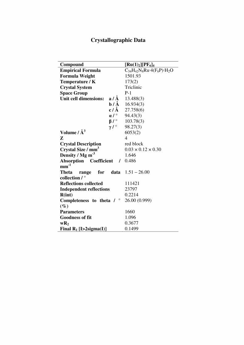
Crystallographic Data

Compound [Ru(1)2][PF6]4 Empirical Formula C54H42N8Ru·4(F6P)·H2O

Formula Weight 1501.93

Temperature / K 173(2)

Crystal System Triclinic

Space Group P-1

Unit cell dimensions: a / Å 13.488(3)

b / Å 16.934(3)

c / Å 27.758(6)

α / ° 94.43(3)

β / ° 103.78(3)

γ / ° 98.27(3)

Volume / Å3 6053(2)

Z 4

Crystal Description red block

Crystal Size / mm3 0.03 × 0.12 × 0.30

Density / Mg m-3 1.646

Absorption Coefficient / mm-1

0.486

Theta range for data collection / °

1.51 – 26.00

Reflections collected 111421

Independent reflections 23797

R(int) 0.2214

Completeness to theta / ° (%)

26.00 (0.999)

Parameters 1660

Goodness of fit 1.096

wR2 0.3677

Final R1 [I>2sigma(I)] 0.1499

Compound [Ru(3)2][PF6]4 Empirical Formula C476H0N70Ru8O58·F242P46

Formula Weight 14456.64

Temperature / K 173(2)

Crystal System Triclinic

Space Group P -1

Unit cell dimensions: a / Å 17.279(3)

b / Å 17.415(3)

c / Å 50.947(10)

α / ° 98.35(3)

β / ° 93.85(3)

γ / ° 90.77(3)

Volume / Å3 15130(5)

Z 1

Crystal Description Red blocks

Crystal Size / mm3 0.05 × 0.25 × 0.40

Density / Mg m-3 1.587

Absorption Coefficient / mm-1 0.457

Theta range for data collection / °

0.8383 – 0.9775

Reflections collected 294313

Independent reflections 64172

R(int) 0.1260

Completeness to theta / ° (%) 26.88 (0.985)

Parameters 2470

Goodness of fit 0.937

wR2 0.2809

Final R1 [I>2sigma(I)] 0.1061

Compound [Ru(4)2][PF6]4 Empirical Formula C44H38N8Ru·4(F6P)·H2O

Formula Weight 1377.79

Temperature / K 173(2)

Crystal System Monoclinic

Space Group P21/c

Unit cell dimensions: a / Å 18.322(4)

b / Å 8.8509(18)

c / Å 31.688(6)

α / ° 90.00

β / ° 95.16(3)

γ / ° 90.00

Volume / Å3 5117.9(18)

Z 4

Crystal Description red needle

Crystal Size / mm3 0.03 × 0.04 × 0.35

Density / Mg m-3 1.786

Absorption Coefficient / mm-1

0.565

Theta range for data collection / °

2.39 – 27.00

Reflections collected 84418

Independent reflections 11159

R(int) 0.1627

Completeness to theta / ° (%)

27.00 (0.998)

Parameters 925

Goodness of fit 1.161

wR2 0.1385

Final R1 [I>2sigma(I)] 0.0664

Compound [Ru(6)2][PF6]4 Empirical Formula 4(C46H38N8Ru)·16(F6P)·

5 (C2H3N)·3(H2O)

Formula Weight 5795.09

Temperature / K 173(2)

Crystal System Monoclinic

Space Group Cc

Unit cell dimensions: a / Å 25.5529(9)

b / Å 15.1322(7)

c / Å 16.2770(7)

α / ° 90.00

β / ° 117.0660(10)

γ / ° 90.00

Volume / Å3 5604.6(4)

Z 1

Crystal Description red block

Crystal Size / mm3 0.15 × 0.25 × 0.45

Density / Mg m-3 1.715

Absorption Coefficient / mm-

1 0.521

Theta range for data collection / °

Reflections collected 47951

Independent reflections 12829

R(int) 0.0372

Completeness to theta / ° (%) 27.50 (0.998)

Parameters 942

Goodness of fit 1.049

wR2 0.1132

Final R1 [I>2sigma(I)] 0.0467

Compound [Ru(7)2][PF6]4 Empirical Formula C56H62F24N8OP4Ru

Formula Weight 1544.09

Temperature / K 123(2)

Crystal System Triclinic

Space Group P -1

Unit cell dimensions: a / Å 8.7018(7)

b / Å 12.5549(10)

c / Å 30.067(3)

α / ° 91.770(6)

β / ° 95.442(6)

γ / ° 98.367(6)

Volume / Å3 3231.88

Z 2

Crystal Description red needle

Crystal Size / mm3 0.03 × 0.08 × 0.45

Density / Mg m-3 1.587

Absorption Coefficient / mm-1 0.457

Theta range for data collection / °

0.8207 to 0.9864

Reflections collected 42067

Independent reflections 11406

R(int) 0.1005

Completeness to theta / ° (%) 25.05 (0.996)

Parameters 1060

Goodness of fit 1.118

wR2 0.3352

Final R1 [I>2sigma(I)] 0.1312

Compound 9 Empirical Formula C50H38N4

Formula Weight 694.88

Temperature / K 100

Crystal System Orthorhombic

Space Group Pbca

Unit cell dimensions: a / Å 8.9360(3)

b / Å 15.3904(5)

c / Å 26.8164(9)

α / ° 90

β / ° 90

γ / ° 90

Volume / Å3 3688.0(2)

Z 4

Crystal Description yellow plate

Crystal Size / mm3 0.020 × 0.100 × 0.220

Density / Mg m-3 1.251

Absorption Coefficient / mm-

1 0.565

Theta range for data collection / °

3.296 to 68.471

Reflections collected 35364

Independent reflections 3377

R(int) 0.068

Completeness to theta / ° (%) 67.102 (0.998)

Parameters 244

Goodness of fit 1.0410

wR2 0.0384

Final R1 [I>2sigma(I)] 0.0478

Compound [Cu(8)2][PF6]

Empirical Formula C24H24Cu1F6N4P1

Formula Weight 576.99

Temperature / K 123

Crystal System Monoclinic

Space Group P21/c

Unit cell dimensions: a / Å 12.7104(6)

b / Å 21.9632(11)

c / Å 8.7001(5)

α / ° 90

β / ° 94.692(2)

γ / ° 90

Volume / Å3 2420.6(2)

Z 4

Crystal Description red block

Crystal Size / mm3 0.060 × 0.130 × 0.210

Density / Mg m-3 1.583

Absorption Coefficient / mm-1 1.036

Theta range for data collection / °

1.856 to 32.588

Reflections collected 35645

Independent reflections 8817

R(int) 0.030

Completeness to theta / ° (%) 32.588 (0.999)

Parameters 325

Goodness of fit 1.0891

wR2 0.0312

Final R1 [I>2sigma(I)] 0.0301

Compound [Cu(9)2][PF6]

Empirical Formula C100H76Cu1F6N8P1

Formula Weight 1666.32

Temperature / K 123

Crystal System Tetragonal

Space Group P4/n

Unit cell dimensions: a / Å 15.1209(2)

b / Å 15.1209(2)

c / Å 18.2971(4)

α / ° 90

β / ° 90

γ / ° 90

Volume / Å3 4183.48(12)

Z 2

Crystal Description orange plate

Crystal Size / mm3 0.030 × 0.170 × 0.210

Density / Mg m-3 1.316

Absorption Coefficient / mm-1

0.352

Theta range for data collection / °

1.747 to 31.714

Reflections collected 49103

Independent reflections 7090

R(int) 0.062

Completeness to theta / ° (%)

31.714 (0.997)

Parameters 276

Goodness of fit 1.0236

wR2 0.0524

Final R1 [I>2sigma(I)] 0.0494

Compound 14 Empirical Formula C18H17N3O

Formula Weight 291.35

Temperature / K 123(2)

Crystal System Monoclinic

Space Group P21/c

Unit cell dimensions: a / Å 7.6803(19)

b / Å 11.193(3)

c / Å 17.011(5)

α / ° 90.00

β / ° 90.329(10)

γ / ° 90.00

Volume / Å3 1462.3(7)

Z 4

Crystal Description colourless needle

Crystal Size / mm3 0.04 × 0.04 × 0.25

Density / Mg m-3 1.323

Absorption Coefficient / mm-1 0.084

Theta range for data collection / °

3.43 to 22.81

Reflections collected 10463

Independent reflections 3006

R(int) 0.0589

Completeness to theta / ° (%) 26.50 (0.992)

Parameters 202

Goodness of fit 1.023

wR2 0.1903

Final R1 [I>2sigma(I)] 0.0780

Compound 15 Empirical Formula C18H15N3

Formula Weight 273.33

Temperature / K 123(2)

Crystal System Monoclinic

Space Group C2/c

Unit cell dimensions: a / Å 31.0692(17)

b / Å 6.5480(4)

c / Å 13.7053(8)

α / ° 90.00

β / ° 100.287(3)

γ / ° 90.00

Volume / Å3 2743.4(3)

Z 8

Crystal Description colourless block

Crystal Size / mm3 0.05 × 0.30 × 0.30

Density / Mg m-3 1.324

Absorption Coefficient / mm-

1 0.080

Theta range for data collection / °

3.08 to 27.49

Reflections collected 32903

Independent reflections 3144

R(int) 0.0271

Completeness to theta / ° (%) 27.49 (0.996)

Parameters 191

Goodness of fit 1.032

wR2 0.0955

Final R1 [I>2sigma(I)] 0.0360

Compound Co-crystallised 15 and 17 Empirical Formula C18H15N3O0.31

Formula Weight 278.31

Temperature / K 123(2)

Crystal System Monoclinic

Space Group P21/c

Unit cell dimensions: a / Å 6.2417(2)

b / Å 8.6472(3)

c / Å 26.2360(10)

α / ° 90.00

β / ° 92.017(2)

γ / ° 90.00

Volume / Å3 1415.16(9)

Z 4

Crystal Description yellow block

Crystal Size / mm3 0.15×0.20×0.40

Density / Mg m-3 1.306

Absorption Coefficient / mm-1 0.081

Theta range for data collection / °

3.11 to 33.07

Reflections collected 12728

Independent reflections 3101

R(int) 0.0210

Completeness to theta / ° (%) 27.10(0.996)

Parameters 202

Goodness of fit 1.047

wR2 0.1053

Final R1 [I>2sigma(I)] 0.0398

Compound 16 Empirical Formula C12H10N2O2

Formula Weight 214.22

Temperature / K 123

Crystal System Monoclinic

Space Group P21/c

Unit cell dimensions: a / Å 3.8672(14)

b / Å 10.873(4)

c / Å 23.976(9)

α / ° 90.00

β / ° 93.974(4)

γ / ° 90.00

Volume / Å3 1005.7(6)

Z 4

Crystal Description colourless needle

Crystal Size / mm3 0.020 × 0.030 × 0.310

Density / Mg m-3 1.415

Absorption Coefficient / mm-1 0.099

Theta range for data collection / °

2.058 to 26.371

Reflections collected 6134

Independent reflections 2053

R(int) 0.108

Completeness to theta / ° (%) 26.371(1.000)

Parameters 145

Goodness of fit 1.1003

wR2 0.0688

Final R1 [I>2sigma(I)] 0.0626

Compound [Cu(15)2][PF6] Empirical Formula C72H69Cu2F12N12O4.50P2

Formula Weight 1591.44

Temperature / K 123(2)

Crystal System Triclinic

Space Group P-1

Unit cell dimensions: a / Å 11.497(2)

b / Å 12.283(2)

c / Å 14.749(3)

α / ° 96.949(11)

β / ° 112.804(10)

γ / ° 103.550(12)

Volume / Å3 1813.6(6)

Z 1

Crystal Description Red plate

Crystal Size / mm3 0.02 × 0.10 × 0.45

Density / Mg m-3 1.452

Absorption Coefficient / mm-1

0.719

Theta range for data collection / °

2.02 to 25.05

Reflections collected 23159

Independent reflections 6379

R(int) 0.0916

Completeness to theta / ° (%)

25.05 (0.991)

Parameters 490

Goodness of fit 1.029

wR2 0.2050

Final R1 [I>2sigma(I)] 0.0769

Jennifer Amy Rudd (née Paley) MChem Hons AMRSC

Email: jpaley530@googlemail.com Date of Birth: 12th

August 1987

Education and Qualifications:

Oct. 2009 – Universität Basel, Basel, Switzerland

Nov. 2012 Studied for a PhD in coordination chemistry in the Housecroft/Constable

research group. Techniques used include UV-vis and emission

spectroscopy, lifetime measurements, spectroelectrochemistry, cyclic

voltammetry (inc. square wave and DPV), NMR, DFT and TD-DFT.

Have supervised two Wahlpraktikum students and assisted in the First

Year undergraduate teaching laboratories for three years.

Proficient in the use of Microsoft Office applications. Basic Linux

experience. Familiar with DFT tools: Gaussian 09, GaussSum, Molekel,

Molden, GaussView.

2005 – 2009 University of York, York, UK

MChem Year Abroad (2:2) inc. Option Modules in Natural

Environment, Clean Technology, Radicals in Synthesis, Catalysis.

Final year at Münster Universität, Germany working in the Hahn

research group on N-heterocyclic carbenes which included the use of air

sensitive compounds, glove box techniques and a Schlenk line.

1998-2005 Hayesfield School Technology College, Bath

A Levels: Chemistry (C), Mathematics (C), German (D), Music (B)

GCSEs: 8(A); 2(B); 1(C)

Technical Experience

2008 Student Researcher, University of York, York (7 weeks)

o Worked in Prof. Perutz’s research group synthesising organometallic

iridium catalysts for asymmetric hydrogenation.

o Synthesised two novel iridium complexes and characterised them using 1H,

13C and

19F NMR, ESI Mass spectrometry, IR spectroscopy, UV-vis

spectroscopy and X-ray crystallography.

2006 Student Scientist, Vectura Plc, Chippenham (8 weeks)

o Worked as part of a team on a project researching dry powder inhalers.

o Job was split between secretarial work and work in the laboratory.

o Laboratory work included making up solutions, cleaning glassware and

making up solutions for the HPLC machine.

2005 Work Experience, Hunstman Petrochemicals, ICI Plant, Teeside (1 week)

o Shadowed chemists working on petroleum purity and zeolite catalysts.

o Went on 2 site visits to see the production of paraxylene and cyclohexane.

Interests and Activities

• Secretary for the Swiss Young Chemist’s Association: responsibilities include

taking the minutes of the meetings, aiding organization of the Snow Symposium

with a particular responsibility for the speakers.

• Associate member of the Royal Society of Chemistry.

• Student member of the Swiss Chemical Society, affiliate of the Photochemistry

section.

• Responsible for running a youth group called Rock Solid for 11-14 year olds at

the International School Basel in Reinach, Baselland.

• Worship Leader and singer at Anglican Church Basel

Additional Skills

• Attained LFA Level 5 (highest offered) German through the University of York

and retain a working knowledge of the language.

Referees

Prof. Dr. E. C. Constable, University of Basel, Basel, Switzerland

Tel: (0041) 61 2671001 Email: edwin.constable@unibas.ch

Prof. Dr. C. E. Housecroft, University of Basel, Switzerland

Tel: (0041) 61 2671018 Email: catherine.housecroft@unibas.ch

Publications:

B. Bozic-Weber, V. Chaurin, E.C. Constable, C.E. Housecroft, M. Meuwly, M.

Neuburger, J.A. Rudd, E. Schönhofer, L. Siegfried, “Exploring copper(I)-based dye-

sensitized solar cells: a complementary experimental and TD-DFT investigation” Dalton

Trans., 2012, 41, 14157-14169

E.C. Constable, M. Devereux, E.L. Dunphy, C.E. Housecroft, J.A. Rudd, J.A. Zampese,

“Water-soluble alkylated bis4'-(4-pyridyl)-2,2':6',2")-terpyridineruthenium(II)

complexes for use as photosensitizers in water oxidation: a complementary experimental

and TD-DFT investigation” Dalton Trans., 2011, 40, 5505-5515

M. C. Jahnke, J. Paley, F. Hupka, J. J. Weigand, F. E. Hahn, “Silver and Gold Complexes

with Benzimidazolin-2-ylidene Ligands”, Z. Naturforsch. 2009, 64b, 1458 – 1462

Poster and Oral Presentations:

“Copper(I) Complexes for Application in Dye-Sensitised Solar Cells: A Comparative

Experimental and TD-DFT Investigation”

Nov. 2012 Oral presentation at the 1st Clariant Chemistry Day, University of Basel (CH)

June 2012 Poster and Flash Poster presentation presented at the Dalton Summer

School on Electronic Structural Methods in Inorganic Chemistry,

University of Edinburgh, UK.

February 2012 Poster Presentation at the Central European Conference on

Photochemistry 2012, Bad Hofgastein, Austria

“Water-soluble alkylated bis4'-(4-pyridyl)-2,2':6',2"-terpyridineruthenium(II)

complexes for use as photosensitizers in water oxidation: a complementary experimental

and TD-DFT investigation”

September 2011 Poster Presentation at the 5th

EuCheMS Nitrogen Ligands conference,

Granada, E

September 2011 Poster presentation at the SCS Fall Meeting, Lausanne, CH

“Photophysical and electrochemical investigations of functionalised bis 4'-pyridyl-

2,2':6',2"-terpyridine Ru(II) complexes”

February 2011 Oral Presentation at the 9th

Swiss Snow Symposium, Lenk, CH

September 2010 Poster Presentation at the SCS Fall Meeting, Zurich, CH

August 2010 Poster Presentation at the 3rd EuCheMS Conference, Nuernberg, DE

An oral presentation of the poster was then featured in the Wiley

electronic magazine “Chemistry Views” (05.10.10)

June 2010 Poster and Flash Poster presentation presented at the Dalton Summer

School on Electronic Structural Methods in Inorganic Chemistry,

University of Edinburgh, UK.