Embed Size (px)
Citation preview
Trajectory Generation Using Cubic Curvature Polynomials
Yuliang Li2017-4
Clemson University
Index
• Trajectory Generation Problem
• Method for trajectory generation
• Experiments & Examples
• Future work
• References

Before we start
History of this algorithm
• 2001, Introduced by Nagy, Bryan, and Alonzo Kelly.
• 2007, Boss the autonomous vehicle, CMU (winner of DARPA ’ 07)
• 2011, McNaughton’s PhD Thesis, CMU
• 2015, Open-Source project CPFL-Autoware
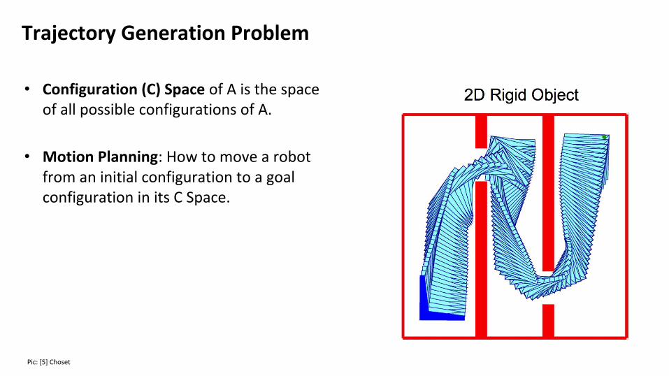
Trajectory Generation Problem
• Configuration (C) Space of A is the space of all possible configurations of A.
• Motion Planning: How to move a robot from an initial configuration to a goal configuration in its C Space.
Pic: [5] Choset
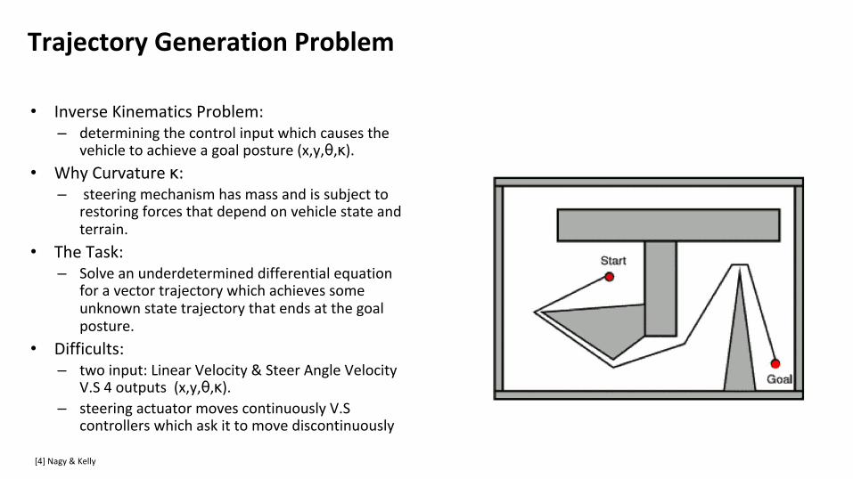
Trajectory Generation Problem
• Inverse Kinematics Problem: – determining the control input which causes the
vehicle to achieve a goal posture (x,y,θ,κ).
• Why Curvature κ:– steering mechanism has mass and is subject to
restoring forces that depend on vehicle state and terrain.
• The Task:– Solve an underdetermined differential equation
for a vector trajectory which achieves some unknown state trajectory that ends at the goal posture.
• Difficults: – two input: Linear Velocity & Steer Angle Velocity
V.S 4 outputs (x,y,θ,κ).
– steering actuator moves continuously V.S controllers which ask it to move discontinuously
[4] Nagy & Kelly
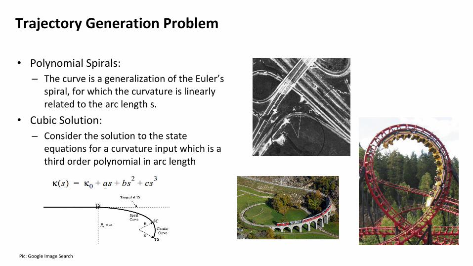
Trajectory Generation Problem
• Polynomial Spirals:– The curve is a generalization of the Euler’s
spiral, for which the curvature is linearly related to the arc length s.
• Cubic Solution:– Consider the solution to the state
equations for a curvature input which is a third order polynomial in arc length
Pic: Google Image Search
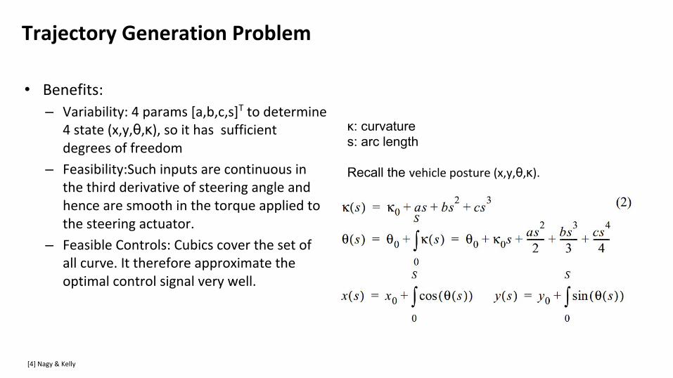
Trajectory Generation Problem
• Benefits:– Variability: 4 params [a,b,c,s]T to determine
4 state (x,y,θ,κ), so it has sufficient degrees of freedom
– Feasibility:Such inputs are continuous in the third derivative of steering angle and hence are smooth in the torque applied to the steering actuator.
– Feasible Controls: Cubics cover the set of all curve. It therefore approximate the optimal control signal very well.
[4] Nagy & Kelly
κ: curvatures: arc length
Recall the vehicle posture (x,y,θ,κ).
Trajectory Generation Problem
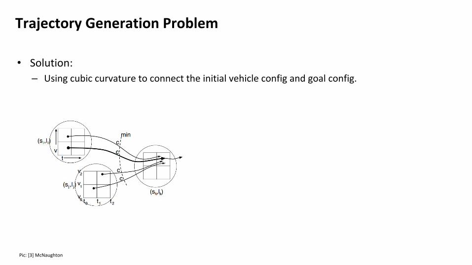
• Solution:– Using cubic curvature to connect the initial vehicle config and goal config.
Pic: [3] McNaughton
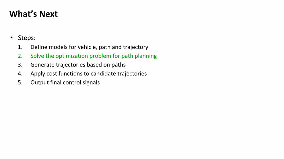
What’s Next
• Steps:1. Define models for vehicle, path and trajectory
2. Solve the optimization problem for path planning
3. Generate trajectories based on paths
4. Apply cost functions to candidate trajectories
5. Output final control signals
Models
• Vehicle: – config of posture (x,y,θ,κ)
• Path:– A path is a continuous function ρ mapping the interval [0,1] into a C Space. – ρ:[0,1] -> C– κ(s) = κ
0 + κ
1s + κ
2s2 + κ
3s3
• Trajectory:– A new space M= {(x, y, θ, κ, t, v)}.– Add time the velocity to the path and map the interval into the new space– τ:[0,1] -> Μ
• Curvature:– Assume the vehicle is moving parallel to the road – Calculated from waypoints
[3] McNaughton
What’s Next
• Steps:1. Define models for vehicle, path and trajectory
2. Solve the optimization problem for path planning
3. Generate trajectories based on paths
4. Apply cost functions to candidate trajectories
5. Output final control signals
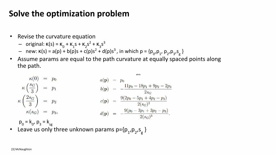
Solve the optimization problem
• Revise the curvature equation– original: κ(s) = κ
0 + κ
1s + κ
2s2 + κ
3s3
– new: κ(s) = a(p) + b(p)s + c(p)s2 + d(p)s3 , in which p = {p0,p
1, p
2,p
3,s
g }
• Assume params are equal to the path curvature at equally spaced points along the path.
p0 = k
0, p
3 = k
sg
• Leave us only three unknown params p={p1,p
2,s
g }
[3] McNaughton
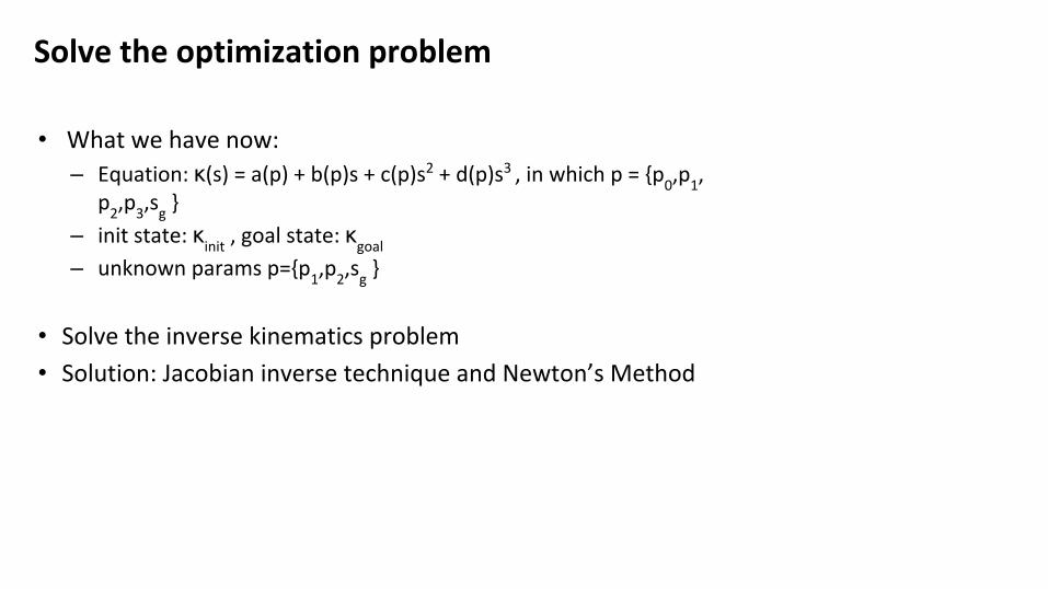
Solve the optimization problem
• What we have now:– Equation: κ(s) = a(p) + b(p)s + c(p)s2 + d(p)s3 , in which p = {p
0,p
1,
p2,p
3,s
g }
– init state: κinit
, goal state: κgoal
– unknown params p={p1,p
2,s
g }
• Solve the inverse kinematics problem
• Solution: Jacobian inverse technique and Newton’s Method
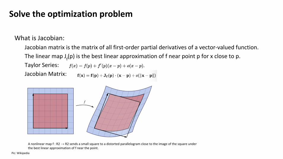
Solve the optimization problem
What is Jacobian:Jacobian matrix is the matrix of all first-order partial derivatives of a vector-valued function.
The linear map Jf(p) is the best linear approximation of f near point p for x close to p.
Taylor Series:
Jacobian Matrix:
A nonlinear map f : R2 → R2 sends a small square to a distorted parallelogram close to the image of the square under the best linear approximation of f near the point.
Pic: Wikipedia
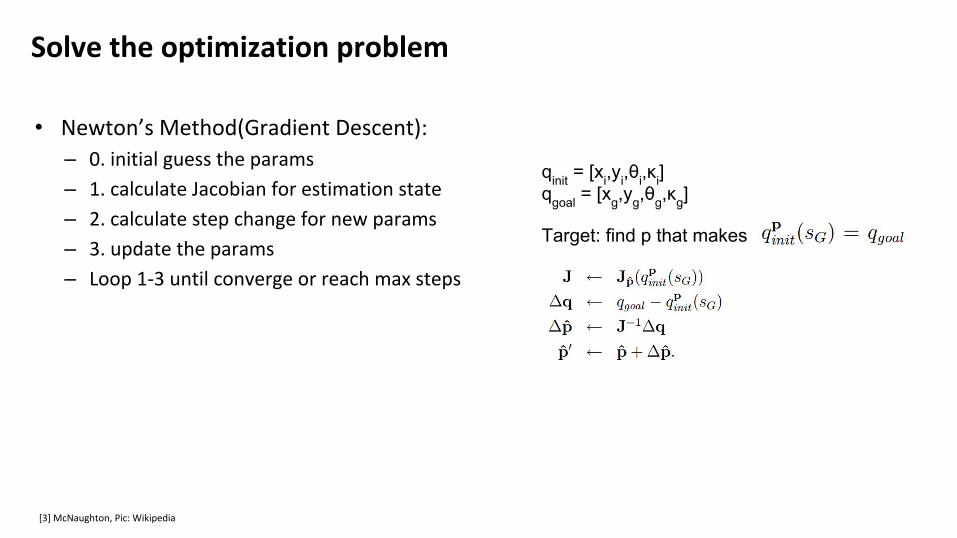
Solve the optimization problem
• Newton’s Method(Gradient Descent):– 0. initial guess the params
– 1. calculate Jacobian for estimation state
– 2. calculate step change for new params
– 3. update the params
– Loop 1-3 until converge or reach max steps
[3] McNaughton, Pic: Wikipedia
Target: find p that makes
qinit = [xi,yi,θi,κi]qgoal = [xg,yg,θg,κg]
Solve the optimization problem
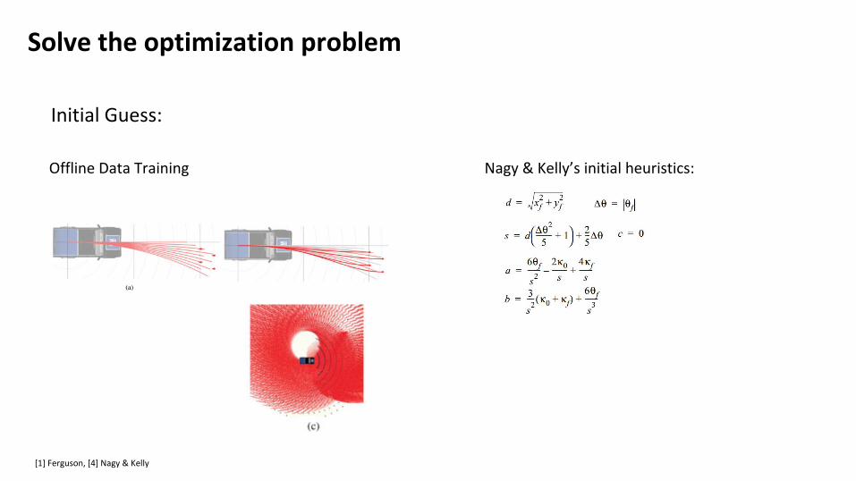
[1] Ferguson, [4] Nagy & Kelly
Nagy & Kelly’s initial heuristics: Offline Data Training
Initial Guess:
Solve the optimization problem
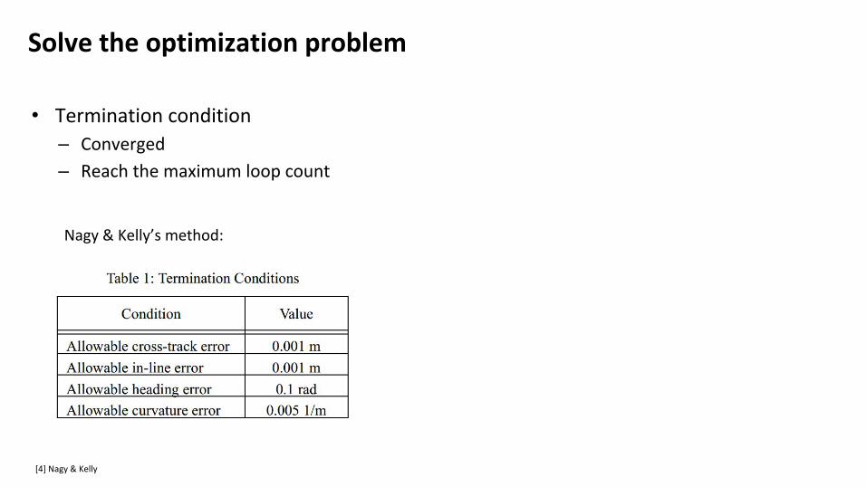
• Termination condition– Converged
– Reach the maximum loop count
[4] Nagy & Kelly
Nagy & Kelly’s method:
Path Results
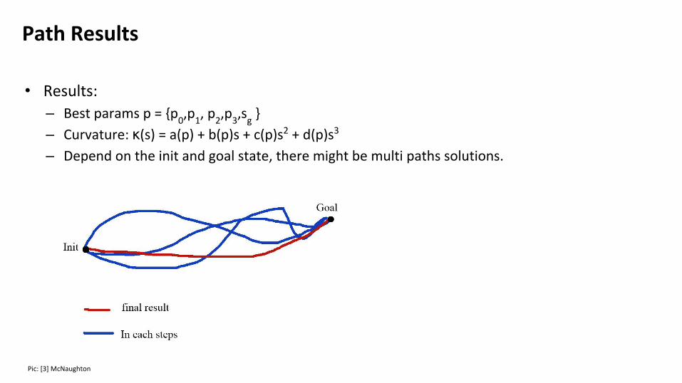
• Results:– Best params p = {p
0,p
1, p
2,p
3,s
g }
– Curvature: κ(s) = a(p) + b(p)s + c(p)s2 + d(p)s3
– Depend on the init and goal state, there might be multi paths solutions.
Pic: [3] McNaughton
What’s Next
• Steps:1. Define models for vehicle, path and trajectory.
2. Solve the optimization problem for path planning
3. Generate trajectories based on paths
4. Apply cost functions to candidate trajectories
5. Output final control signals
Trajectories Generation
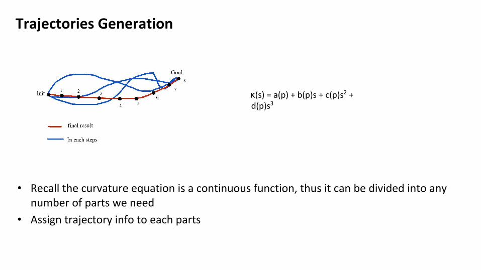
• Recall the curvature equation is a continuous function, thus it can be divided into any number of parts we need
• Assign trajectory info to each parts
κ(s) = a(p) + b(p)s + c(p)s2 + d(p)s3
Trajectories Generation
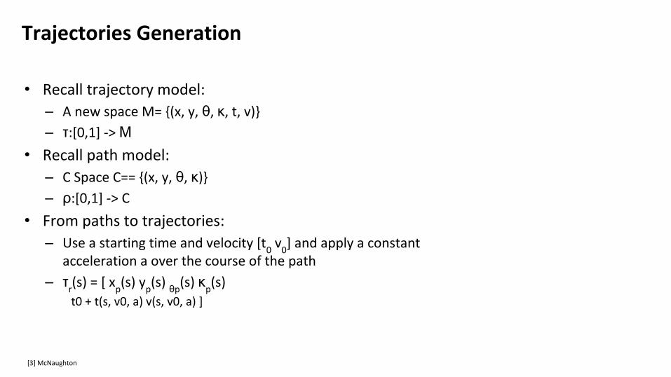
• Recall trajectory model:– A new space M= {(x, y, θ, κ, t, v)}
– τ:[0,1] -> Μ• Recall path model:
– C Space C== {(x, y, θ, κ)}
– ρ:[0,1] -> C
• From paths to trajectories:– Use a starting time and velocity [t
0 v
0] and apply a constant
acceleration a over the course of the path
– τr(s) = [ x
p(s) y
p(s) θp
(s) κp(s)
t0 + t(s, v0, a) v(s, v0, a) ]
[3] McNaughton
Trajectories Generation
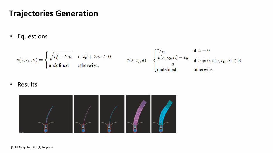
• Equestions
• Results
[3] McNaughton Pic: [1] Ferguson
What’s Next
• Steps:1. Define models for vehicle, path and trajectory.
2. Solve the optimization problem for path planning
3. Generate trajectories based on paths
4. Apply cost functions to candidate trajectories
5. Output final control signals
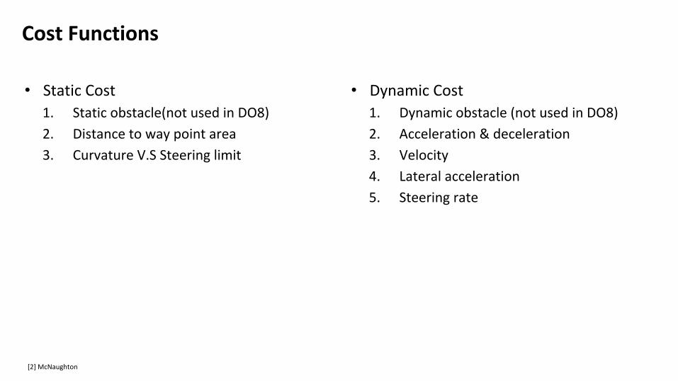
Cost Functions
• Static Cost1. Static obstacle(not used in DO8)
2. Distance to way point area
3. Curvature V.S Steering limit
• Dynamic Cost1. Dynamic obstacle (not used in DO8)
2. Acceleration & deceleration
3. Velocity
4. Lateral acceleration
5. Steering rate
[2] McNaughton
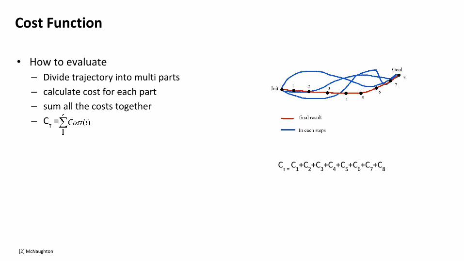
Cost Function
• How to evaluate – Divide trajectory into multi parts
– calculate cost for each part
– sum all the costs together
– Cτ =
Cτ = C
1+C
2+C
3+C
4+C
5+C
6+C
7+C
8
[2] McNaughton
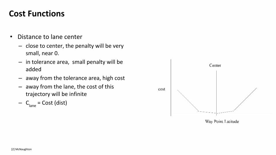
Cost Functions
• Distance to lane center– close to center, the penalty will be very
small, near 0.
– in tolerance area, small penalty will be added
– away from the tolerance area, high cost
– away from the lane, the cost of this trajectory will be infinite
– Clane
= Cost (dist)
[2] McNaughton
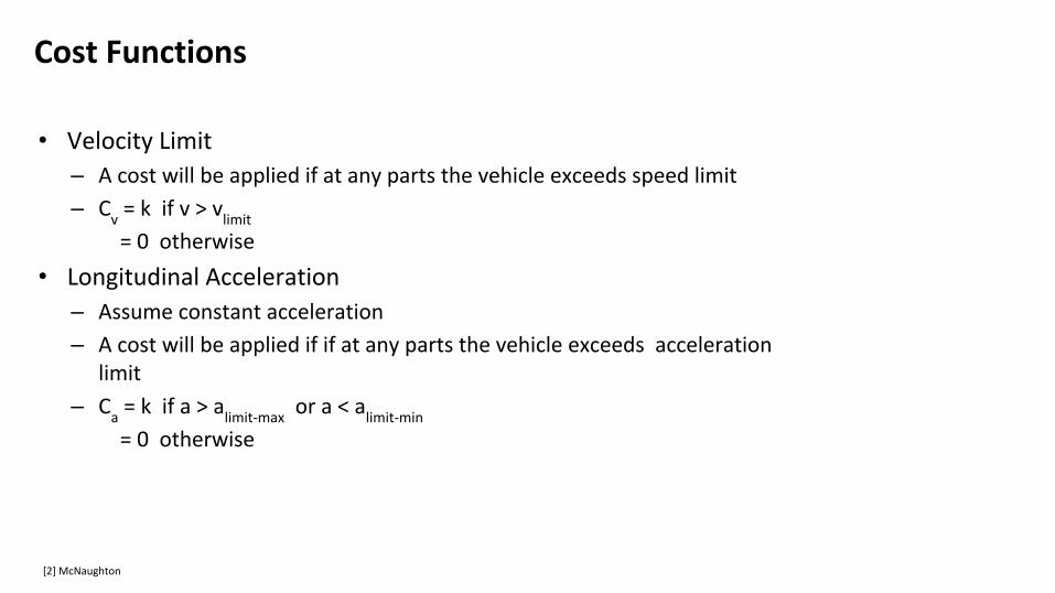
Cost Functions
• Velocity Limit– A cost will be applied if at any parts the vehicle exceeds speed limit
– Cv = k if v > v
limit
= 0 otherwise
• Longitudinal Acceleration– Assume constant acceleration
– A cost will be applied if if at any parts the vehicle exceeds acceleration limit
– Ca = k if a > a
limit-max or a < a
limit-min
= 0 otherwise
[2] McNaughton
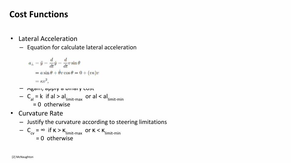
Cost Functions
• Lateral Acceleration– Equation for calculate lateral acceleration
– Again, apply a binary cost– C
al = k if al > al
limit-max or al < al
limit-min
= 0 otherwise
• Curvature Rate– Justify the curvature according to steering limitations– C
cv = ∞ if κ > κ
limit-max or κ < κ
limit-min
= 0 otherwise
[2] McNaughton
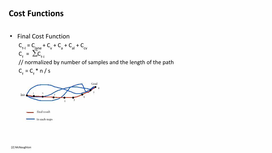
Cost Functions
• Final Cost FunctionCτ-I
= Clane
+ Cv + C
a + C
al + C
cv
Cτ = Cτ-i
// normalized by number of samples and the length of the path
Cτ = Cτ
* n / s
[2] McNaughton
What’s Next
• Steps:1. Define models for vehicle, path and trajectory.
2. Solve the optimization problem for path planning
3. Generate trajectories based on paths
4. Apply cost functions to candidate trajectories
5. Output final control signals
Trajectories to Control Signals
• Deal with control delays– Control Delay: Latency in the vehicle’s physical response to the actuator commands.
– Planning Latency: From the generation timestamp to the final vehicle movement.
• Example: In 2011, CMU’s BOSS – Control delay: 80ms
– Planning Latency: 200ms
[1] Ferguson
Trajectories to Control Signals
• Trajectories Queue– Vector based function [x, y, θ, t,v, a
1,a
2] over time interval [t
0 t
f ]
– Recall our results are continuous functions, here we divide the result into discrete parts
– Update cycle: 10 HZ (100ms)
– Send cmd every cycle
– Actual control signal: earlier than “control delay” and no later than” planning latency”
Trajectories to Control Signals
• More to research– Fixed Frame V.S Rolling Frame
– Deviation between planner and vehicle motion
Pseudo Code
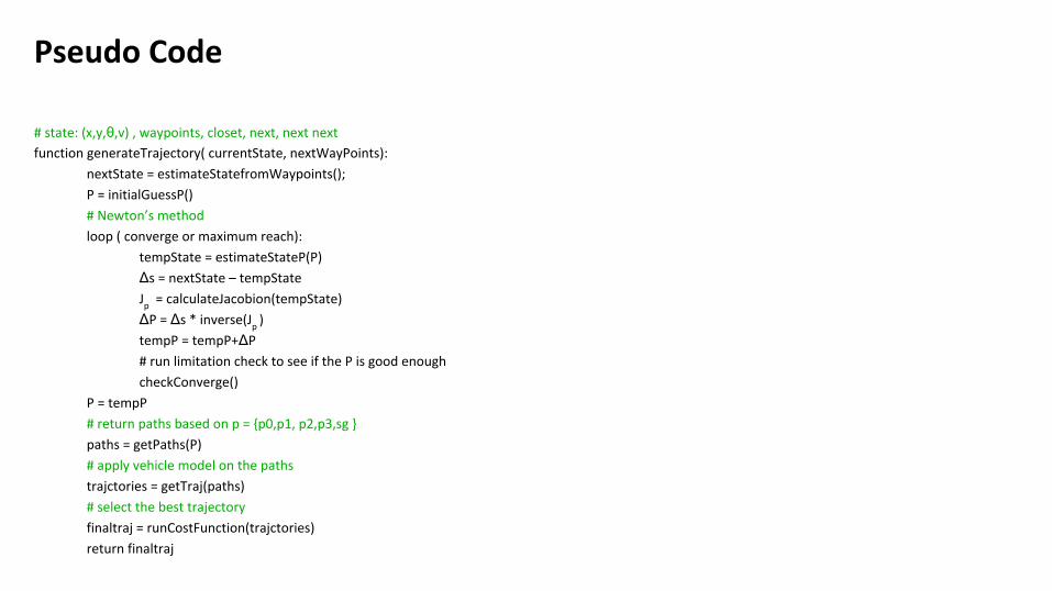
# state: (x,y,θ,v) , waypoints, closet, next, next next
function generateTrajectory( currentState, nextWayPoints):
nextState = estimateStatefromWaypoints();
P = initialGuessP()
# Newton’s method
loop ( converge or maximum reach):
tempState = estimateStateP(P)
Δs = nextState – tempState
Jp = calculateJacobion(tempState)
ΔP = Δs * inverse(Jp
)
tempP = tempP+ΔP
# run limitation check to see if the P is good enough
checkConverge()
P = tempP
# return paths based on p = {p0,p1, p2,p3,sg }
paths = getPaths(P)
# apply vehicle model on the paths
trajctories = getTraj(paths)
# select the best trajectory
finaltraj = runCostFunction(trajctories)
return finaltraj
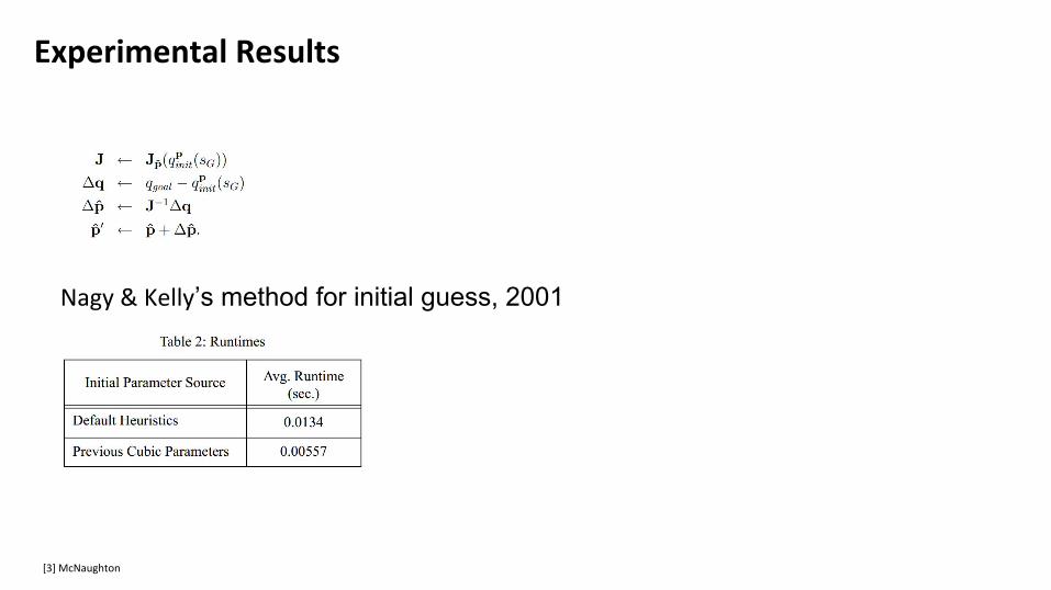
Experimental Results
[3] McNaughton
Nagy & Kelly’s method for initial guess, 2001
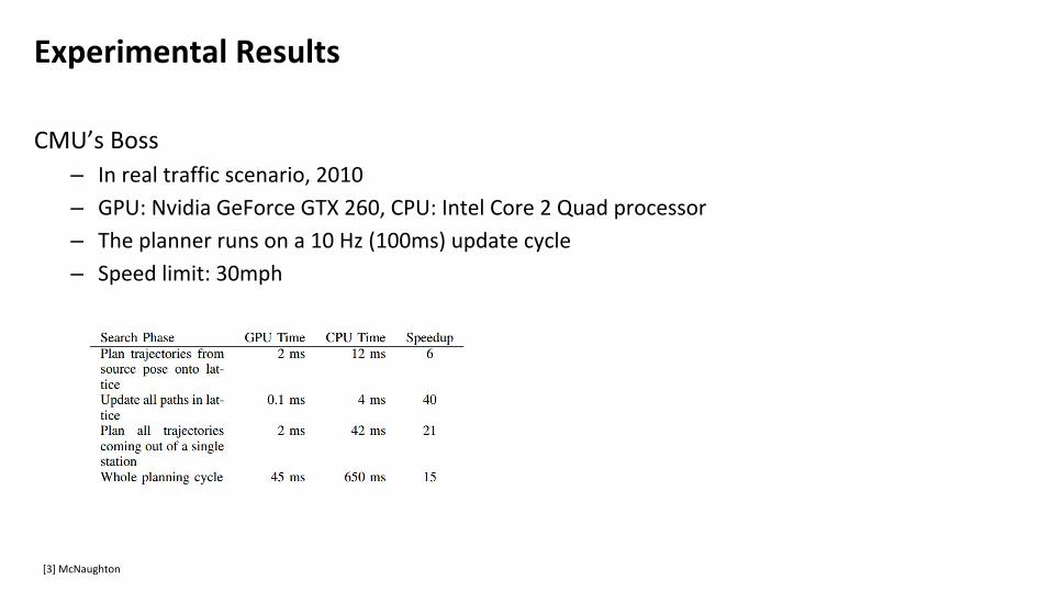
Experimental Results
CMU’s Boss– In real traffic scenario, 2010
– GPU: Nvidia GeForce GTX 260, CPU: Intel Core 2 Quad processor
– The planner runs on a 10 Hz (100ms) update cycle
– Speed limit: 30mph
[3] McNaughton
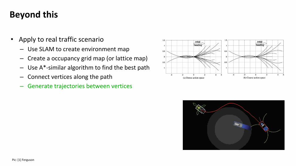
Beyond this
• Apply to real traffic scenario– Use SLAM to create environment map
– Create a occupancy grid map (or lattice map)
– Use A*-similar algorithm to find the best path
– Connect vertices along the path
– Generate trajectories between vertices
Pic: [1] Ferguson
References
• [1] Ferguson, Dave, Thomas M. Howard, and Maxim Likhachev. "Motion planning in urban environments." Journal of Field Robotics 25.11-12 (2008): 939-960.
• [2] McNaughton, Matthew. "Parallel algorithms for real-time motion planning." (2011).
• [3] McNaughton, Matthew, et al. "Motion planning for autonomous driving with a conformal spatiotemporal lattice." Robotics and Automation (ICRA), 2011 IEEE International Conference on. IEEE, 2011.
• [4] Nagy, Bryan, and Alonzo Kelly. "Trajectory generation for car-like robots using cubic curvature polynomials." Field and Service Robots 11 (2001).
• [5] Choset, Robotic Motion Planning: Configuration Space
• [6] Baker, Christopher R., David I. Ferguson, and John M. Dolan. "Robust mission execution for autonomous urban driving." Robotics Institute (2008): 178.
About
• I wrote this document in order to study the trajectory planning method used in CMU’s Boss the autonomous driving car.
• Matthew O’Kelly, who wrote the Autoware’s trajectory planning module, helped me a lot during my study on this. Thank you!
• And the next might be something based on this algorithm using C++ or Python. In summer break 2017.