Polynomial-time counting and sampling of two-rowed contingency tables

Theoretical Computer Science 246 (2000) 265–278www.elsevier.com/locate/tcs

Polynomial-time counting and samplingof two-rowed contingency tables(

Martin Dyer, Catherine Greenhill ∗

School of Computer Studies, University of Leeds, Leeds, LS2 9JT, UK

Received May 1998; revised January 1999Communicated by M.S. Paterson

Abstract

In this paper a Markov chain for contingency tables with two rows is de�ned. The chain isshown to be rapidly mixing using the path coupling method. We prove an upper bound for themixing time of the chain. The upper bound is quadratic in the number of columns and linearin the logarithm of the table sum. By considering a speci�c problem, we prove a lower boundfor the mixing time of the chain. The lower bound is quadratic in the number of columns andlinear in the logarithm of the number of columns. A fully polynomial randomised approximationscheme for this problem is described. c© 2000 Published by Elsevier Science B.V. All rightsreserved.

Keywords: Randomized algorithms; Contigency tables; Markov chains; Complexity;Path coupling

1. Introduction

A contingency table is a matrix of nonnegative integers with prescribed positive rowand column sums. Contingency tables are used in statistics to store data from samplesurveys (see for example [3, Chapter 8]). For a survey of contingency tables and relatedproblems, see [8]. The data is often analysed under the assumption of independence.If the set of contingency tables under consideration is small, this assumption can betested by applying a chi-squared statistic to each such table (see for example [1, 7, 20]).However, this approach becomes computationally infeasible as the number of contin-gency tables grows. Suppose that we had a method for sampling almost uniformly from

( An earlier version of this paper appeared in the 25th Annual EATCS International Colloquium onAutomata, Languages and Programming, July 1998.

∗ Corresponding author.E-mail address: [email protected] (C. Greenhill).

0304-3975/00/$ - see front matter c© 2000 Published by Elsevier Science B.V. All rights reserved.PII: S0304 -3975(99)00136 -X

266 M. Dyer, C. Greenhill / Theoretical Computer Science 246 (2000) 265–278

the set of contingency tables with given row and column sums. Then we may proceedby applying the statistic to a sample of contingency tables selected almost uniformly.The problem of almost uniform sampling can be e�ciently solved using the Markov

chain Monte Carlo method (see [16]), provided that there exists a Markov chain forthe set of contingency tables which converges to the uniform distribution in polyno-mial time. Here ‘polynomial time’ means ‘in time polynomial in the number of rows,the number of columns and the logarithm of the table sum’. If the Markov chainconverges in time polynomial in the table sum itself, then we shall say it convergesin pseudopolynomial time. Approximately counting two-rowed contingency tables ispolynomial-time reducible to almost uniform sampling, as we prove in Section 3. More-over, the problem of exactly counting the number of contingency tables with �xed rowand column sums is known to be #P-complete, even when there are only two rows(see [13]).The �rst Markov chain for contingency tables was described in [9] by Diaconis and

Salo�-Coste. We shall refer to this chain as the Diaconis chain. For �xed dimensions,they proved that their chain converges in pseudopolynomial time. However, the con-stants involved grow exponentionally with the number of rows and columns. SomeMarkov chains for restricted classes of contingency tables have been de�ned. In [17],Kannan et al. gave a Markov chain with polynomial-time convergence for the 0–1 case(where every entry in the table is zero or one) with nearly equal margin totals, whileChung et al. [6] described a Markov chain for contingency tables which convergesin pseudopolynomial time for contingency tables with large enough margin totals. Animprovement on this result is the chain described by Dyer et al. [13]. Their chainconverges in polynomial time whenever all the row and column sums are su�cientlylarge, this bound being smaller than that in [6].In [15], Hernek analysed the Diaconis chain for two-rowed contingency tables us-

ing coupling. She showed that this chain converges in time which is quadratic in thenumber of columns and in the table sum (i.e. pseudopolynomial time). In this paper,a new Markov chain for two-rowed contingency tables is described, and the conver-gence of the chain is analysed using the path coupling method [4]. We show that thenew chain converges to the uniform distribution in time which is quadratic in the num-ber of columns and linear in the logarithm of the table sum. Therefore, our chain runsin (genuinely) polynomial time, whereas the Diaconis chain does not (and indeed can-not). By considering a speci�c example, we prove a lower bound for the new Markovchain which is quadratic in the number of columns and linear in the logarithm of thenumber of columns.The structure of the remainder of the paper is as follows. In the next section the path

coupling method is reviewed. In Section 3 we introduce notation for contingency tablesand show that approximate counting of two-rowed contingency tables is polynomial-time reducible to almost uniform sampling. We describe the Diaconis chain, whichconverges in pseudopolynomial time. Although this chain can be used for approximatecounting, we present a procedure which can perform exact counting for two-rowedcontingency tables in pseudopolynomial time. A new Markov chain for two-rowed

M. Dyer, C. Greenhill / Theoretical Computer Science 246 (2000) 265–278 267

contingency tables is described in Section 4 and the mixing time is analysed usingpath coupling. The new chain is the �rst which converges in genuinely polynomialtime for all two-rowed contingency tables. A lower bound for the mixing time of thischain is developed in Section 5.

2. A review of path coupling

In this section we present some necessary notation and review the path couplingmethod. Let be a �nite set and letM be a Markov chain with state space , transitionmatrix P and unique stationary distribution �. If the initial state of the Markov chainis x then the distribution of the chain at time t is given by Ptx (y)=P

t(x; y). The totalvariation distance of the Markov chain from � at time t, with initial state x, is de�nedby

dTV(Ptx ; �)=12∑y∈

|P t(x; y)− �(y)|:

A Markov chain is only useful for almost uniform sampling or approximate countingif its total variation distance can be guaranteed to tend to zero relatively quickly, givenany initial state. Let �x(�) denote the least value T such that dTV(Ptx ; �)6� for allt¿T . Following Aldous [2], the mixing time of M, denoted by �(�), is de�ned by�(�)=max{�x(�): x∈}. A Markov chain will be said to be rapidly mixing if themixing time is bounded above by some polynomial in log(||) and log(�−1), wherethe logarithms are to base e.There are relatively few methods available to prove that a Markov chain is rapidly

mixing. One such method is coupling. A coupling forM is a stochastic process (Xt; Yt)on × such that each of (Xt); (Yt), considered marginally, is a faithful copy ofM. The Coupling lemma (see for example, Aldous [2]) states that the total variationdistance of M at time t is bounded above by Prob[Xt 6=Yt], the probability that theprocess has not coupled. The di�culty in applying this result lies in obtaining an upperbound for this probability. In the path coupling method, introduced by Bubley andDyer [4], one need only de�ne and analyse a coupling on a subset S of ×. Choosingthe set S carefully can considerably simplify the arguments involved in proving rapidmixing of Markov chains by coupling. The path coupling method is described in thenext theorem, taken from Dyer and Greenhill [12]. Here we use the term path to referto a sequence of elements in the state space, which need not form a sequence ofpossible transitions of the Markov chain.

Theorem 2.1. Let � be an integer-valued metric de�ned on × which takes valuesin {0; : : : ; D}. Let S be a subset of × such that for all (Xt; Yt)∈× there existsa path

Xt =Z0; Z1; : : : ; Zr =Yt


between Xt and Yt where (Zl; Zl+1)∈ S for 06l¡r and∑r−1

l= 0 �(Zl; Zl+1)= �(Xt; Yt).De�ne a coupling (X; Y ) 7→ (X ′; Y ′) of the Markov chain M on all pairs (X; Y )∈ S.Suppose that there exists �¡1 such that

E[�(X ′; Y ′)]6� �(X; Y )

for all (X; Y )∈ S. Then the mixing time �(�) of M satis�es

�(�)6log(D�−1)1− � :

3. Contingency tables

Let r=(r1; : : : ; rm) and s=(s1; : : : ; sn) be two positive integer partitions of the posi-tive integer N . The set �r; s of contingency tables with these row and column sums isde�ned by

�r; s=

{Z ∈Nm×n0 :

n∑j= 1

Zij = ri for 16i6m;m∑i= 1

Zij = sj for 16j6n

}: (1)

The problem of approximately counting the number of contingency tables with givenrow and column sums is known to be #P-complete even when one of m, n equals 2(see [13, Theorem 1]). However the 2×2 problem can be solved exactly, as describedbelow.For 2×2 contingency tables we introduce the notationT ca; b=�(a; c−a); (b; c−b);

where 0¡a; b¡c. Now

T ca; b={[

i (a− i)(b− i) (c + i − a− b)

]: max{0; a+ b− c}6i6 min{a; b}

}:

Hence

|T ca; b|={min{a; b}+ 1 if a+ b6c;c −max{a; b}+ 1 if a+ b¿c:

(2)

Choosing an element uniformly at random from T ca; b is accomplished simply by choos-ing i∈{max{0; a+ b− c} ; : : : ;min{a; b}} uniformly at random and forming the corre-sponding element of T ca; b; that is, the element of T

ca; b with i in the north–west corner.

For the remainder of the section, we consider two-rowed contingency tables. Herem=2, and r=(r1; r2); s=(s1; : : : ; sn) are positive integer partitions of the positiveinteger N . We now show that approximately counting two-rowed contingency tableswith given row and column sums is polynomial-time reducible to almost uniform sam-pling. First, let us make this statement more precise. Let �, � be such that 0¡�; �¡1.A fully polynomial randomised approximation scheme (or FPRAS) [18] for |�r; s| is a


randomised algorithm which runs in time polynomial in n, log(N ), �−1 and log(�−1)to produce an estimate Z for |�r; s|, such that

Prob[(1− �)|�r; s|6Z6(1 + �)|�r; s|]¿1− �:Suppose that M is a rapidly mixing Markov chain for two-rowed contingency tables,and let �(�) denote the mixing time of M. Then �(�) is bounded above by a polynomialin n, log(N ) and log(�−1). We now describe an FPRAS for �r; s which uses the Markovchain M to perform almost uniform sampling from �r; s. This FPRAS di�ers from mostof the known schemes for other combinatorial problems, as its complexity depends uponnumber size (that is, the column sums themselves and not just the number of columns).For this reason, we present a brief description. Some proof details are omitted, as thearguments involved are standard [10, 16].Let R be de�ned by R=

∑nq= 3dlog2(sq)e. Then R¡n log(N ). We estimate |�r; s| in

R steps, and only describe the �rst step in detail. Let Uj be de�ned by

Uj = {X ∈�r; s: Xjn¿dsn=2e}for j=1; 2. Let M be de�ned by

M = d150e2R2�−2 log(3R�−1)e:Using the Markov chain M, produce a sample S ⊆�r; s of size M as follows:

S := ∅;let x be some arbitrarily chosen element of �r; s;let T := �(�=(15Re2));for j := 1 to M doperform T steps of the Markov chain M, starting from initial state x;let S := S ∪{X }, where X is the �nal state of the chain;

enddo;

De�ne J ∈{1; 2} by

J ={1 if |S ∩U1|¿M=2;2 otherwise:

Let Z1 = |S ∩UJ |M−1. Then Z1¿ 12 . We take Z1 as our estimate for �1, where �1 =

|UJ‖�r; s|−1. Let r′ be obtained from r by subtracting dsn=2e from rJ . Finally, let s′ bede�ned by

s′={(s1; : : : ; sn−1; bsn=2c) if sn¿1;(s1; : : : ; sn−1) if sn=1:

Then |UJ |= |�r′ ; s′ |, so this quantity can be estimated using the same method. Theprocess terminates after R steps, where it remains to calculate the number of 2×2contingency tables with given row and column sums. Let � be this number, whichcan be evaluated exactly. Let Zi be the estimate for �i which we obtain at the ith


step. Then Z=�(Z1 · · ·ZR)−1 is our estimate for |�r; s|, while |�r; s|=�(�1 · · · �R)−1 byconstruction.We now outline the steps involved in proving that this procedure is indeed an

FPRAS. Let �̂i=E[Zi] for 16i6R. By choice of M and the simulation length ofthe Markov chain, we can prove the following:

(i) for 16i6R; |�i − �̂i|6�=(15Re2),(ii) for 16i6R; Prob[�̂i¿1=(2e

2)]¿1− �=(3R),(iii) if �̂i¿1=(2e

2) for some i such that 16i6R, then |�i − �̂i|6�=(5R)�̂i,(iv) if �̂i¿1=(2e

2) for some i such that 16i6R, then

Prob[|Zi − �̂i|¿�=(5R)�̂i]62�=(3R);(v) with probability at least 1− �, we have

|(Z1 : : : ZR)−1 − (�1 : : : �R)−1|6�(�1 : : : �R)−1:It is now not di�cult to see that

Prob[(1− �)|�r; s|6Z6(1 + �)|�r; s|]¿1− �:(The structure of this argument is standard, see [10, 16].) Thus, with high enoughprobability, we have estimated |�r; s| to within the required accuracy.In order to estimate the complexity of this procedure, assume that the mixing time

of the Markov chain used in the ith step of the procedure is bounded above by �(�),the mixing time of the Markov chain used in the �rst step. This is reasonable since thenumber of columns is non-increasing as the procedure progresses. The total number ofMarkov chain simulations used in this procedure is bounded above by

RM�(�=(15Re2)):

Since M is rapidly mixing, and by de�nition of M and R, this expression is polynomialin n; log(N ), �−1 and log(�−1). This proves the existence of an FPRAS for approxi-mately counting contingency tables. In other words, approximate counting of two-rowedcontingency tables is polynomial-time reducible to almost uniform sampling.We now describe a well-known Markov chain for two-rowed contingency tables.

In [9], the following Markov chain for two-rowed contingency tables was introduced.We refer to this chain as the Diaconis chain. Let r=(r1; r2) and s=(s1; : : : ; sn) be twopositive integer partitions of the positive integer N . If the current state of the Diaconischain is X∈�r; s, then the next state X ′∈�r; s is produced using the following procedure:with probability 1

2 , let X′=X . Otherwise, choose (j1; j2) uniformly at random such

that 16j1¡j26n, and choose i∈{1;−1} uniformly at random. Form X ′ from X byadding the matrix[

i −i−i i

]

to the 2×2 submatrix of X consisting of the j1th and j2th columns of X . If X ′ =∈�r; sthen let X ′=X . It is not di�cult to see that this chain is ergodic with uniform stationary


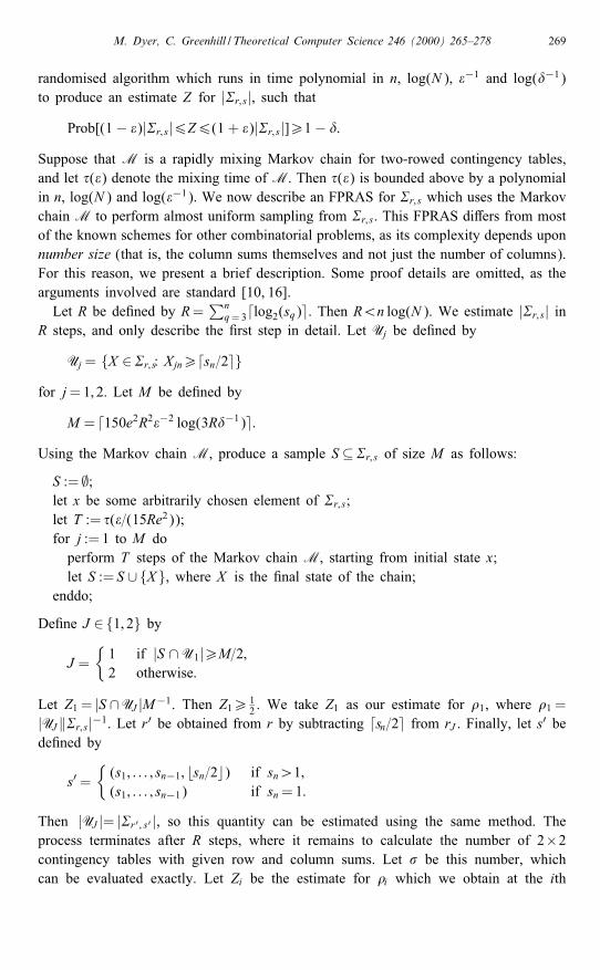
distribution (see, for example [15]). This chain was analysed using coupling by Hernek[15]. She proved that the chain is rapidly mixing with mixing rate quadratic in thenumber of columns n and in the table sum N . Hence the Diaconis chain converges inpseudopolynomial time.To close this section, we show how to calculate |�r; s| exactly using O(nN ) oper-

ations. The method, due to Diane Hernek [14], is an e�cient dynamic programmingapproach based on a certain recurrence. This shows that exact counting is achievablein pseudopolynomial time, and approximate counting is only of value if it can beachieved in polynomial time. The new chain described in the next section is the �rstMarkov chain for general two-rowed contingency tables which provably converges inpolynomial time.Let R=min{r1; r2}, and for 16i6R; 16j6n let

Sij ={(x1; : : : ; xj):

j∑k = 1

xk = i and 06xk6sk for 16k6j}:

Let Aij = |Sij| for 06i6R, 06j6n. Then |�r; s|=ARn. Let A0j =1 for 06j6n, andlet Ai0 = 0 for 16i6R. It is not di�cult to show that the following recurrence holds:

Aij ={Ai; j−1 + Ai−1; j if i − 1¡sj;Ai; j−1 + Ai−1; j − Ai−sj−1;j−1 if i − 1¿sj:

This leads to the following O(nN )-time algorithm for calculating |�r; s|.Beginfor j := 0 to n doA0j := 1;

endfor;for i := 1 to R doAi0 := 0;

endfor;for i := 1 to R dofor j := 1 to n doAij :=Ai; j−1 + Ai−1; j;if i − 1¿sj thenAij :=Aij − Ai−sj−1; j−1;

endif;endfor;

endfor;return ARn;

End.

As mentioned above, this procedure has running time O(nN ). Thus it saves a factor ofnN compared with the best-known upper bound of O(n2N 2) for the cost of generatinga single sample from �r; s using the Diaconis chain.


4. A new Markov chain for two-rowed contingency tables

For this section assume that m=2. A new Markov chain for two-rowed contingencytables will now be described. First we must introduce some notation. Suppose thatX∈�r; s where r=(r1; r2). Given (j1; j2) such that 16j1¡j26n let TX (j1; j2) denotethe set T ca; b where a=X1; j1 + X1; j2 , b= sj1 and c= sj1 + sj2 . Then TX (j1; j2) is the setof 2×2 contingency tables with the same row and column sums as the 2×2 submatrixof X consisting of the j1th and j2th columns of X . (Here the row sums may equalzero.) Let M(�r; s) denote the Markov chain with state space �r; s with the followingtransition procedure. If Xt is the state of the chain M(�r; s) at time t then the state attime t + 1 is determined as follows:(i) choose (j1; j2) uniformly at random such that 16j1¡j26n,(ii) choose x∈TX (j1; j2) uniformly at random and let

Xt+1(k; j)={x(k; l) if j= jl for l∈{1; 2};X t(k; j) otherwise

for 16k62, 16j6n.Clearly M(�r; s) is aperiodic. Now M(�r; s) can perform all the moves of the

Diaconis chain, and the Diaconis chain is irreducible (see [15]). Therefore M(�r; s)is irreducible, so M(�r; s) is ergodic. Given X; Y ∈�r; s let

�(X; Y )=n∑j=1

|X1; j − Y1; j|:

Then � is a metric on �r; s which only takes as values the even integers in the range{0; : : : ; N}. Denote by �(X; Y ) the minimum number of transitions of M(�r; s) requiredto move from initial state X to �nal state Y . Then

06�(X; Y )6�(X; Y )=2 (3)

using moves of the Diaconis chain only (see [15]). However, these bounds are far fromtight, as the following shows. Let K(X; Y ) be the number of columns which di�er inX and Y . The following result gives a bound on �(X; Y ) in terms of K(X; Y ) only.

Lemma 4.1. If X; Y ∈�r; s and X 6=Y thendK(X; Y )=2e6�(X; Y )6K(X; Y )− 1:

Proof. Consider performing a series of transitions of M(�r; s), starting from initialstate X and relabelling the resulting state by X each time, with the aim of decreas-ing K(X; Y ). Each transition of M(�r; s) can decrease K(X; Y ) by at most 2. Thisproves the lower bound. Now X 6=Y so K(X; Y )¿2. Let j1 be the least value ofj such that X and Y di�er in the jth column. Without loss of generality supposethat X1; j1¿Y1; j1 . Then let j2 be the least value of j¿j1 such that X1; j¡Y1; j. Letx=min {X1; j1 − Y1; j1 ; Y1; j2 − X1; j2}. In one move of M(�r; s) we may decrease X1; j1


and X2; j2 by x and increase X1; j2 and X2; j1 by x. This decreases K(X; Y ) by at least 1.The decrease in K(X; Y ) is 2 whenever X1; j1 −Y1; j1 =Y1; j2 −X1; j2 . This is certainly thecase when K(X; Y )= 2, proving the upper bound.

This result shows that the diameter of M(�r; s) is at most (n− 1). Now (3) impliesthat the diameter of the Diaconis chain is at most bN=2c. By considering the set of2× 2 contingency tables with row and column sums given by (bN=2c; dN=2e), we seethat bN=2c is also a lower bound for the diameter of the Diaconis chain; that is, thediameter of the Diaconis chain is exactly bN=2c. In many cases, N is much larger thann, suggesting that the new chain M(�r; s) might be considerably more rapidly mixingthan the Diaconis chain in these situations. The transition matrix P of M(�r; s) hasentries

P(X; Y )=

∑j1¡j2 ((

n2 )|TX ( j1; j2)|)−1 if X =Y;

(( n2 )|TX ( j1; j2)|)−1 if X; Y di�er in j1th;

j2th columns only;

0 otherwise:

If all di�erences between X and Y are contained in the j1th and j2th columns onlythen TX ( j1; j2)=TY ( j1; j2). Hence P is symmetric and the stationary distribution ofM(�r; s) is the uniform distribution on �r; s. The Markov chain M(�r; s) is an exampleof a heat bath Markov chain, as described in [5]. We now prove that M(�r; s) israpidly mixing using the path coupling method on the set S of pairs (X; Y ) such that�(X; Y )= 2.

Theorem 4.1. Let r=(r1; r2) and s=(s1; : : : ; sn) be two positive integer partitions ofthe positive integer N . The Markov chain M(�r; s) is rapidly mixing with mixingtime �(�) satisfying

�(�)6n(n− 1)

2log(N�−1):

Proof. Let X and Y be any elements of �r; s. It was shown in [15] that there exists apath

X =Z0; Z1; : : : ; Zd=Y (4)

such that �(Zl; Zl+1)= 2 for 06l¡d and Zl ∈�r; s for 06l6d, where d=�(X; Y )=2.Now assume that �(X; Y )= 2. Without loss of generality,

Y =X +[−1 1 0 · · · 0

1 −1 0 · · · 0

]:

We must de�ne a coupling (X; Y ) 7→ (X ′; Y ′) for M(�r; s) at (X; Y ). Let ( j1; j2) bechosen uniformly at random such that 16j1¡j26n. If ( j1; j2)= (1; 2) or 36j1¡j26n


then TX ( j1; j2)=TY ( j1; j2). Here we de�ne the coupling as follows: let x∈TX ( j1; j2)be chosen uniformly at random and let X ′ (respectively Y ′) be obtained from X (re-spectively Y ) by replacing the jlth column of X (respectively Y ) with the lth columnof x, for l=1; 2. If ( j1; j2)= (1; 2) then �(X ′; Y ′)= 0, otherwise �(X ′; Y ′)= 2.It remains to consider indices ( j1; j2) where j1 ∈ {1; 2} and 36j26n. Without loss

of generality, suppose that ( j1; j2)= (2; 3). Let TX =TX (2; 3) and let TY =TY (2; 3). Leta=X1;2 + X1;3, b= s2 and c= s2 + s3. Then

TX =Tca; b and TY =Tca+1; b:

Suppose that a+ b¿c. Then relabel the rows of X and Y and swop the labels of thesecond and third columns of X and Y . Finally interchange the roles of X and Y . Leta′; b′; c′ denote the resulting parameters. Then

a′ + b′=(c − a− 1) + (c − b)= c − (a+ b− c)− 1¡c= c′:

Therefore, we may assume without loss of generality, that a + b¡c. There are twocases depending on which of a or b is the greater.Suppose �rst that a¿b. Then

TX ={[

iX (a− iX )(b− iX ) (c + iX − a− b)

]: 06iX6b

}

and

TY ={[

iY (a+ 1− iY )(b− iY ) (c + iY − a− b− 1)

]: 06iY6b

}:

Choose iX ∈ {0; : : : ; b} uniformly at random and let iY = iX . Let X ′ (respectively Y ′)be obtained from X (respectively Y ) by replacing the jlth column of X (respectivelyY ) with the lth column of x (respectively y) for l=1; 2. This de�nes a coupling ofM(�r; s) at (X; Y ) for this choice of ( j1; j2). Here �(X ′; Y ′)= 2.Suppose next that a¡b. Then

TX ={[

iX (a− iX )(b− iX ) (c + iX − a− b)

]: 06iX6a

}

and

TY ={[

iY (a+ 1− iY )(b− iY ) (c + iY − a− b− 1)

]: 06iY6a+ 1

}:

Choose iX ∈ {0; : : : ; a} uniformly at random and let

iY ={iX with probability (a− iX + 1)(a+ 2)−1;iX + 1 with probability (iX + 1)(a+ 2)−1:


If i∈ {0; : : : ; a+ 1} thenProb [iY = i] = Prob [iX = i] · (a− i + 1)(a+ 2)−1

+Prob [iX = i − 1] · ((i − 1) + 1)(a+ 2)−1= (a+ 1)−1((a− i + 1)(a+ 2)−1 + i(a+ 2)−1)= (a+ 2)−1:

Therefore each element of {0; : : : ; a+ 2} is equally likely to be chosen, and the couplingis valid. Let x be the element of TX which corresponds to iX and let y be the element ofTY which corresponds to iY . Let X ′, Y ′ be obtained from X , Y as above. This de�nesa coupling of M(�r; s) at (X; Y ) for this choice of ( j1; j2). Again, �(X ′; Y ′)= 2.Putting this together, it follows that

E[�(X ′; Y ′)]= 2

(1−

(n2

)−1)¡2=�(X; Y ):

Let �=1 − (n2)−1. We have shown that E[�(X ′; Y ′)]= ��(X; Y ), and clearly �¡1.Therefore M(�r; s) is rapidly mixing, by Theorem 2.1. Since �(X; Y )6N for all X;Y ∈�r;w the mixing time �(�) satis�es

�(�)6n(n− 1)

2log(N�−1);

as stated.

Attempts have been made to extend this Markov chain to act on general m-rowedcontingency tables, so far without success. The problem seems much harder, even whenrestricted to three-rowed contingency tables. See [11] for more details.

5. A lower bound for the mixing time

In this section we �nd a lower bound for the mixing time of the Markov chain M

for two-rowed contingency tables. We proceed by considering a speci�c sequence ofcontingency tables, de�ned below. In the chosen example we have N =2(n− 1), andwe prove the lower bound

n(n− 1)6

log(n− 18

)6�(e−1):

Taking the upper and lower bounds together shows that

�(e−1)=�(n2 log(n))

for this example. Of course we do not always have N =�(n). It is not known whether,in general, the upper bound O(n2 log(N )) is tight, or whether (n2 log(n)) is the correctlower bound.


We now de�ne the set of contingency tables to be considered. It is the set �r; s ofcontingency tables with row sums r=(n−1; n−1) and column sums s=(n−1; 1; : : : ; 1).Suppose that X ∈�r; s. Then 06X116n−1. Moreover, there are exactly

(n−1i

)elements

X ∈�r; s such that X11 = i. It follows easily that |�r; s|=2n−1. The distribution of thetop-left element X11 is binomial when X is selected uniformly at random from �r; s.We analyse the sequence {Xk} obtained by simulating the Markov chain M(�r; s),

starting from the initial state X0 given by

X0 =[

0 1 · · · 1n− 1 0 · · · 0

]: (5)

We will focus particularly on the top-left element of each member of this sequence. Forthis reason, let {Yk} be the sequence de�ned by Yk =(Xk)11 for k¿0. Then 06Yk6n− 1 for k¿0. Informally, the distribution of Xk cannot be close to uniform until thedistribution of Yk is close to binomial.Let

�=1− 2n(n− 1) :

Using standard methods, it is possible to prove that

E[Yk ] =n− 12(1− �k) (6)

for k¿0. Hence {E [Yk ]} is an increasing sequence with limit (n− 1)=2, the expectedvalue in the binomial distribution. Again using standard methods, one can prove that

var(Yk)=n− 14(1− (n− 1) �2k + (n− 2) (2� − 1)k) (7)

for k¿0. In particular, var(Yk)6(n − 1)=4 for all k¿0. Using these results, we canprove the following lower bound on the mixing time.

Theorem 5.1. Let �(�) denote the mixing time of the Markov chain M(�r; s). Then

n(n− 1)6

log(n− 18

)6�(e−1):

Proof. Recall the set �r; s de�ned at the start of this section, and the initial state X0,de�ned in (5). Let Pk denote the distribution of the Markov chain M(�r; s), afterperforming k steps from initial state X0. Denote by � the uniform distribution on �r; s,and let dk =dTV(Pk; �), the total variation distance between � and Pk . We bound dkfrom below by comparing the probability that the top-left element of X is at least(n − 1)=2, when X is chosen according to � and Pk , respectively. Formally, let S bede�ned by

S = {X ∈�r; s: X11¿(n− 1)=2} :


Then |�(S) − Pk(S)|6dk , by de�nition of total variation distance. Clearly �(S)¿ 12 .

Using Chebyshev’s bound and standard arguments, it is possible to show that

Pk(S)61

(n− 1)� 2k ;

where �=1− 2=(n(n− 1)). Therefore12− 1(n− 1)� 2k6|�(S)− Pk(S)|6dk :

Suppose that k = �(e−1), where �(�) is the mixing time of the Markov chain �r; s. Thendk6e−1, which implies that

12− 1(n− 1)� 2k6e

−1:

After some rearranging, this implies that

k¿� log((n− 1)=8)

2(1− �) ¿n(n− 1)

6log(n− 18

):

Here the �nal inequality uses the fact that �¿ 23 . This proves the theorem.

Taking the lower bound for �(e−1) proved in Theorem 5.1, together with the upperbound for the mixing time proved in 4.1, we see that �(e−1)=�(n2 log(n)). In thechosen example, the table sum N satis�es N =�(n). Therefore, this lower bound doesnot tell us whether the log(n) term should be log(N ) in general, or whether (n2 log(n))is the true lower bound. We conjecture that �(n2 log(n)) is true in general, for thefollowing reason. We feel that if every 2×2 submatrix has been visited some constantnumber of times, then this should ensure that the resulting table is very close to random.This requires �(n2 log(n)) steps, by results for the coupon-collectors problem (see, forexample [19, pp. 57–63]).

References

[1] J.H. Albert, A.K. Gupta, Estimation in contingency tables using prior information, J. Roy. Statist. Soc.Ser. B (Methodological) 45 (1) (1983) 60–69.

[2] D. Aldous, Random walks on �nite groups and rapidly mixing Markov chains, in: A. Dold, B. Eckmann(Eds.), S�eminaire de Probabilit�es XVII 1981=1982, Lecture Notes in Mathematics, Vol. 986, Springer,New York, 1983, pp. 243–297.

[3] R. Barlow, Statistics, Wiley, Chichester, 1989.[4] R. Bubley, M. Dyer, Path coupling: A technique for proving rapid mixing in Markov chains, 38th

Annual Symp. on Foundations of Computer Science, IEEE, San Alimitos, 1997, pp. 223–231.[5] R. Bubley, M. Dyer, C. Greenhill, Beating the 2� bound for approximately counting colourings:

A computer-assisted proof of rapid mixing, in 9th Annual Symp. on Discrete Algorithms, ACM-SIAM,New York-Philadelphia, 1998, pp. 355–363.

[6] F.R.K. Chung, R.L. Graham, S.T. Yau, On sampling with Markov chains, Random Struct. Algorithms9 (1996) 55–77.

[7] P. Diaconis, B. E�ron, Testing for independence in a two-way table: new interpretations of the chi-square statistic (with discussion), Ann. Statist. 13 (1985) 845–913.


[8] P. Diaconis, A. Gangolli, Rectangular arrays with �xed margins, in: D. Aldous, P.P. Varaiya,J. Spencer, J.M. Steele (Eds.), Discrete Probability and Algorithms, IMA Volumes on Mathematicsand its Applications, Vol. 72, Springer, New York, 1995, pp. 15–41.

[9] P. Diaconis, L. Salo�-Coste, Random walk on contingency tables with �xed row and column sums,Tech. Report, Department of Mathematics, Harvard University, 1995.

[10] M. Dyer, A. Frieze, Computing the volume of convex bodies: A case where randomness provably helps,Proc. Symp. in Applied Mathematics, Vol. 44, 1991, pp. 123–169.

[11] M. Dyer, C. Greenhill, A genuinely polynomial time algorithm for sampling two-rowed contingencytables, 25th Internat. Colloq. on Automata, Languages and Programming, Aalborg, Denmark, 1998,pp. 339–350.

[12] M. Dyer, C. Greenhill, A more rapidly mixing Markov chain for graph colourings, Random Struct.Algorithms 13 (1998) 285–317.

[13] M. Dyer, R. Kannan, J. Mount, Sampling contingency tables, Random Struct. Algorithms 10 (1997)487–506.

[14] D. Hernek, Private Communication, 1998.[15] D. Hernek, Random generation of 2 × n contingency tables, Random Struct. Algorithms 13 (1998)

71–79.[16] M. Jerrum, A. Sinclair, The Markov chain Monte Carlo method: an approach to approximate counting

and integration, in: D. Hochbaum (Ed.), Approximation Algorithms for NP-Hard Problems, PWSPublishing, Boston, 1996, pp. 482–520.

[17] R. Kannan, P. Tetali, S. Vempala, Simple Markov chain algorithms for generating bipartite graphs andtournaments, 8th Annual Symp. on Discrete Algorithms, ACM-SIAM, New York-Philadelphia, 1997,pp. 193–200.

[18] R.M. Karp, M. Luby, Monte-Carlo algorithms for enumeration and reliability problems, 24th AnnualSymp. on Foundations of Computer Science, IEEE, San Alimitos, 1983, pp. 56–64.

[19] R. Motwani, P. Raghavan, Randomized Algorithms, Cambridge University Press, Cambridge, 1995.[20] J.N.K. Rao, A.J. Scott, The analysis of categorical data from complex sample surveys: chi-squared

tests for goodness of �t and independence in two-way tables, J. Amer. Statist. Assoc. 76 (374) (1981)221–230.

Documents

Polynomial-time counting and sampling of two-rowed contingency tables