Polynomial-Time Amoeba Neighborhood Membership and Faster

Polynomial-Time Amoeba Neighborhood

Membership and Faster Localized Solving

Eleanor Anthony, Sheridan Grant, Peter Gritzmann, and J. Maurice Rojas

Abstract We derive efficient algorithms for coarse approximation of complex alge-

braic hypersurfaces, useful for estimating the distance between an input polynomial

zero set and a given query point. Our methods work best on sparse polynomials

of high degree (in any number of variables) but are nevertheless completely gen-

eral. The underlying ideas, which we take the time to describe without an excess of

algebraic geometry terminology, come from tropical geometry. We then apply our

methods to finding roots of n×n systems near a given query point, thereby reducing

a hard algebraic problem to high-precision linear optimization. We prove new upper

and lower complexity estimates along the way.

Dedicated to Tien-Yien Li, in honor of his birthday.1 Introduction

As students, we are often asked to draw (hopefully without a calculator) real zero

sets of low degree polynomials in few variables. As scientists and engineers, we

are often asked to count or approximate (hopefully with some computational as-

sistance) real and complex solutions of arbitrary systems of polynomial equations

in many variables. If one allows sufficiently coarse approximations, then the latter

problem is as easy as the former. Our main results clarify this transition from hard-

ness to easiness. In particular, we significantly speed up certain queries involving

distances between points and complex algebraic hypersurfaces (see Theorems 1.4–

1.6 below). We then apply our metric results to finding specially constructed start

systems — dramatically speeding up traditional homotopy continuation methods —

to approximate, or rule out, roots of selected norm (see Section 3).

Eleanor Anthony

Mathematics Department, University of Mississippi, Hume Hall 305, P. O. Box 1848, MS 38677-

1848, e-mail: [email protected] . Partially supported by NSF REU grant DMS-1156589.

Sheridan Grant

Mathematics Department, 640 North College Avenue, Claremont, CA 91711, e-mail: sheri-

[email protected] . Partially supported by NSF REU grant DMS-1156589.

Peter Gritzmann

Fakultat fur Mathematik, Technische Universitat Munchen, D-80290 Munchen, Germany, e-mail:

[email protected] . Work supported in part by the German Research Foundation (DFG).

J. Maurice Rojas

Mathematics Department, Texas A&M University, TAMU 3368, College Station, TX 77843-3368,

e-mail: [email protected] . Partially supported by NSF MCS grant DMS-0915245.

1

2 Eleanor Anthony, Sheridan Grant, Peter Gritzmann, and J. Maurice Rojas

Polynomial equations are ubiquitous in numerous applications, such as algebraic

statistics [29], chemical reaction kinetics [42], discretization of partial differential

equations [28], satellite orbit design [47], circuit complexity [36], and cryptography

[10]. The need to solve larger and larger equations, in applications as well as for the-

oretical purposes, has helped shape algebraic geometry and numerical analysis for

centuries. More recent work in algebraic complexity tells us that many basic ques-

tions involving polynomial equations are NP-hard (see, e.g., [52, 13]). This is by no

means an excuse to consider polynomial equation solving hopeless: Computational

scientists solve problems of near-exponential complexity every day.

Thanks to recent work on Smale’s 17th Problem [8, 14], we have learned that ran-

domization and approximation can be the key to avoiding the bottlenecks present

in deterministic algorithms for solving hard questions involving complex roots of

polynomial systems. Smale’s 17th Problem concerns the average-case complex-

ity of approximating a single complex root of a random polynomial system and is

well-discussed in [60, 61, 54, 55, 56, 57, 58]. Our ultimate goal is to extend this phi-

losophy to the harder problem of localized solving: estimating how far the nearest

root of a given system of polynomials (or intersection of several zero sets) is from a

given point. Here, we start by first approximating the shape of a single zero set, and

then in Section 3 we outline a tropical-geometric approach to localized solving.

Toward this end, let us first recall the natural idea (see, e.g., [65]) of drawing zero

sets on log-paper. In what follows, we let C∗ denote the non-zero complex numbers

and write C[x±1

1 , . . . ,x±1n

]for the ring of Laurent polynomials with complex coeffi-

cients, i.e., polynomials with negative exponents allowed. Also, for any two vectors

u :=(u1, . . . ,uN) and v :=(v1, . . . ,vN) in RN , we use u · v to denote the standard dot

product u1v1 + · · ·+uNvN .

(− log3,0)

(0,− log3)

(2log3,3log3)

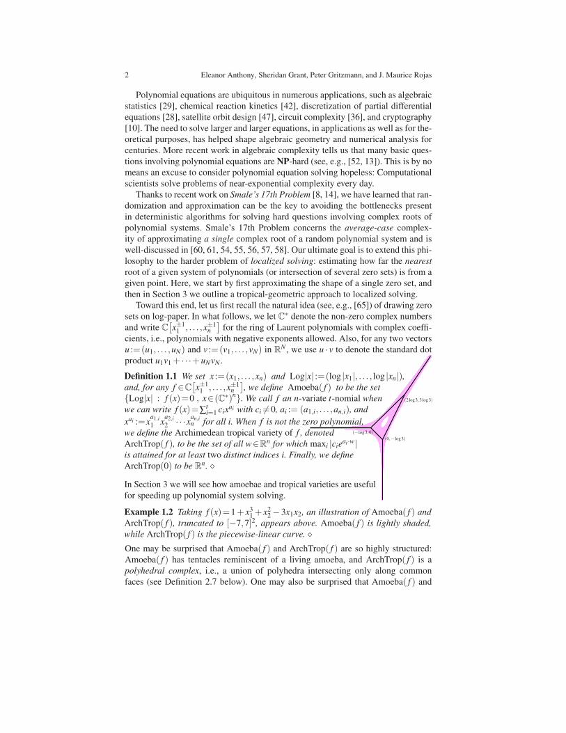
Definition 1.1 We set x :=(x1, . . . ,xn) and Log|x| :=(log |x1|, . . . , log |xn|),and, for any f ∈C

[x±1

1 , . . . ,x±1n

], we define Amoeba( f ) to be the set

{Log|x| : f (x)=0 , x∈(C∗)n}. We call f an n-variate t-nomial when

we can write f (x)=∑ti=1 cix

ai with ci 6=0, ai := (a1,i, . . . ,an,i), and

xai :=xa1,i

1 xa2,i

2 · · ·xan,in for all i. When f is not the zero polynomial,

we define the Archimedean tropical variety of f , denoted

ArchTrop( f ), to be the set of all w∈Rn for which maxi |cieai·w|

is attained for at least two distinct indices i. Finally, we define

ArchTrop(0) to be Rn. ⋄

In Section 3 we will see how amoebae and tropical varieties are useful

for speeding up polynomial system solving.

Example 1.2 Taking f (x)=1+ x31 + x2

2 −3x1x2, an illustration of Amoeba( f ) and

ArchTrop( f ), truncated to [−7,7]2, appears above. Amoeba( f ) is lightly shaded,

while ArchTrop( f ) is the piecewise-linear curve. ⋄One may be surprised that Amoeba( f ) and ArchTrop( f ) are so highly structured:

Amoeba( f ) has tentacles reminiscent of a living amoeba, and ArchTrop( f ) is a

polyhedral complex, i.e., a union of polyhedra intersecting only along common

faces (see Definition 2.7 below). One may also be surprised that Amoeba( f ) and

Faster Amoeba Neighborhoods and Faster Solving 3

ArchTrop( f ) are so closely related: Every point of one set is close to some point of

the other, and both sets have topologically similar complements (4 open connected

components, exactly one of which is bounded). Example 2.2 below shows that we

need not always have ArchTrop( f )⊆Amoeba( f ).To quantify how close Amoeba( f ) and ArchTrop( f ) are in general, one can re-

call the Hausdorff distance, denoted ∆(U,V ), between two subsets U,V ⊆Rn: It is

defined to be the maximum of supu∈U infv∈V |u− v| and supv∈V infu∈U |u− v|. We

then have the following recent result of Avendano, Kogan, Nisse, and Rojas.

Theorem 1.3 [4] Suppose f is any n-variate t-nomial. Then Amoeba( f ) and

ArchTrop( f ) are (a) identical for t ≤ 2 and (b) at Hausdorff distance no greater

than (2t −3) log(t −1) for t≥3. In particular, for t≥2, we also have

supu ∈ Amoeba( f )

infv ∈ ArchTrop( f )

|u− v| ≤ log(t −1).

Finally, for any t>n≥1, there is an n-variate t-nomial f with

∆(Amoeba( f ),ArchTrop( f ))≥ log(t −1). �

Note that the preceding upper bounds are completely independent of the coeffi-

cients, degree, and number of variables of f . Our upcoming examples show that

Amoeba( f ) and ArchTrop( f ) are sometimes much closer than the bound above.

Our first two main results help set the stage for applying Archimedean tropical

varieties to speed up polynomial root approximation. Recall that Q[√−1] denotes

those complex numbers whose real and imaginary parts are both rational. Our com-

plexity results will all be stated relative to the classical Turing (bit) model, with the

underlying notion of input size clarified below in Definition 1.7.

Theorem 1.4 Suppose w∈Rn and f ∈C[x±1

1 , . . . ,x±1n

]is a t-nomial with t≥2. Then

− log(t −1)≤ infu∈Amoeba( f ) |u−w|− infv∈ArchTrop( f ) |v−w|≤(2t −3) log(t −1).

In particular, if we also assume that n is fixed and ( f ,w)∈Q[√−1]

[x±1

1 , . . . ,x±1n

]×

Qn with f a t-nomial, then we can compute polynomially many bits of

infv∈ArchTrop( f ) |v−w| in polynomial-time, and there is a polynomial-time algorithm

that declares either (a) infu∈Amoeba( f ) |u − w| ≤ (2t − 2) log(t − 1) or

(b) w 6∈Amoeba( f ) and infu∈Amoeba( f ) |u−w|≥ infv∈ArchTrop( f ) |v−w|− log(t −1)>0.

Theorem 1.4 is proved in Section 5. The importance of Theorem 1.4 is that deciding

whether an input rational point w lies in an input Amoeba( f ), even restricting to the

special case n=1, is already NP-hard [4].

ArchTrop( f ) naturally partitions Rn into finitely many (relatively open) poly-

hedral cells of dimension 0 through n. We call the resulting polyhedral com-

plex Σ(ArchTrop( f )) (see Definition 2.7 below). In particular, finding the cell of

Σ(ArchTrop( f )) containing a given w∈Rn gives us more information than simply

deciding whether w lies in ArchTrop( f ).

Theorem 1.5 Suppose n is fixed. Then there is a polynomial-time algorithm that,

for any input ( f ,w)∈Q[√

−1][

x±11 , . . . ,x±1

n

]×Qn with f a t-nomial, outputs the

closure of the unique cell σw of Σ(ArchTrop( f )) containing w, described as an

explicit intersection of O(t2) half-spaces.


Theorem 1.5 is proved in Section 4. As a consequence, we can also find explicit

regions, containing a given query point w, where f can not vanish. Let d denote

the degree of f . While our present algorithm evincing Theorem 1.5 has com-

plexity exponential in n, its complexity is polynomial in logd (see Definition 1.7

below). The best previous techniques from computational algebra, including re-

cent advances on Smale’s 17th Problem [8, 14], yield complexity no better than

polynomial in(d+n)!

d!n!≥max

{(d+n

d

)d,(

d+nn

)n}

.

Our framework also enables new positive and negative results on the complexity

of approximating the intersection of several Archimedean tropical varieties.

Theorem 1.6 Suppose n is fixed. Then there is a polynomial-time algorithm that, for

any input k and ( f1, . . . , fk,w)∈(Q[

√−1]

[x±1

1 , . . . ,x±1n

])k ×Qn, outputs the closure

of the unique cell σw of Σ(⋃k

i=1 ArchTrop( fi))

containing w, described as an ex-

plicit intersection of half-spaces. (In particular, whether w lies in⋂k

i=1 ArchTrop( fi)is decided as well.) However, if n is allowed to vary, then deciding whether σw has

a vertex inn⋂

i=1

ArchTrop( fi) is NP-hard.

Theorem 1.6 is proved in Section 6. We will see in Section 3 how the first assertion

of Theorem 1.6 is useful for finding special start-points for Newton Iteration and

Homotopy Continuation that sometimes enable the approximation of just the roots

with norm vector near (ew1 , . . . ,ewn). The final assertion of Theorem 1.6 can be

considered as a refined tropical analogue to a classical algebraic complexity result:

Deciding whether an arbitrary input system of polynomials equations (with integer

coefficients) has a complex root is NP-hard. (There are standard reductions from

known NP-complete problems, such as integer programming or Boolean satisfiabil-

ity, to complex root detection [21, 52].)

On the practical side, we point out that the algorithms underlying Theorems 1.4–

1.6 are quite easily implementable. (A preliminary Matlab implementation of our

algorithms is available upon request.) Initial experiments indicate that a large-scale

implementation could be a worthwhile companion to existing polynomial system

solving software.

Before moving on to the necessary technical background, let us first clarify our

underlying input size and point out some historical context.

Definition 1.7 We define the input size of an integer c to be size(c) := log(2+ |c|)and, for p,q∈Z relative prime with |q|≥ 2, size(p/q) := size(p)+ size(q). Given

a polynomial f ∈Q[x1, . . . ,xn], written f (x)=∑ti=1 cix

ai , we then define size( f ) to

be ∑ti=1

(size(ci)+∑n

j=1 size(ai, j))

, where ai=(ai,1, . . . ,ai,n) for all i. Similarly, we

define the input size of a point (v1, . . . ,vn)∈Qn as ∑ni=1 size(vi). Considering real

and imaginary parts, and summing the respect sizes, we then extend the definition of

input size further still to polynomials in Q[√

−1][x1, . . . ,xn]. Finally, for any system

of polynomials F :=( f1, . . . , fk), we set size(F) :=∑ki=1 size( fi). ⋄

Note in particular that the size of an input in Theorem 1.6 is size(w)+∑ki=1 size( fi).


Remark 1.8 The reader may wonder why we have not considered the phases of the

root coordinates and focussed just on norms. The phase analogue of an amoeba is

the co-amoeba, which has only recently been studied [30, 46, 48]. While it is known

that the phases of the coordinates of the roots of polynomial systems satisfy certain

equidistribution laws (see, e.g., [35, Thm. 1 (pp. 82–83), Thm. 2 (pp. 87–88), and

Cor. 3′ (pg. 88)] and [2]), there does not yet appear to be a phase analogue of

ArchTrop( f ). Nevertheless, we will see in Section 3 that our techniques sometimes

allow us to approximate not just norms of root coordinates but roots in full. ⋄Historical Notes Using convex and/or piecewise-linear geometry to understand

solutions of algebraic equations can be traced back to work of Newton (on power

series expansions for algebraic functions) around 1676 [44].

More recently, tropical geometry [17, 38, 32, 6, 39] has emerged as a rich frame-

work for reducing deep questions in algebraic geometry to more tractable questions

in polyhedral and piecewise-linear geometry. For instance, Gelfand, Kapranov, and

Zelevinsky first observed the combinatorial structure of amoebae around 1994 [22]. ⋄

2 Background

2.1 Convex, Piecewise-Linear, and Tropical Geometric Notions

Let us first recall the origin of the phrase “tropical geometry”, according to [51]:

the tropical semifield Rtrop is the set R ∪ {−∞}, endowed with the operations

x⊙ y :=x+ y and x⊕ y :=max{x,y}. The adjective “tropical” was coined by French

computer scientists, in honor of Brazilian computer scientist Imre Simon, who did

pioneering work with algebraic structures involving Rtrop. Just as algebraic geome-

try relates geometric properties of zero sets of polynomials to the structure of ideals

in commutative rings, tropical geometry relates the geometric properties of certain

polyhedral complexes (see Definition 2.7 below) to the structure of ideals in Rtrop.

Here we work with a particular kind of tropical variety that, thanks to Theorem

1.3, approximates Amoeba( f ) quite well. The binomial case is quite instructive.

Proposition 2.1 For any a∈Zn and non-zero complex c1 and c2, we have

Amoeba(c1 + c2xa)=ArchTrop(c1 + c2xa)={w∈Rn | a ·w= log |c1/c2|}.

Proof: If c1+c2xa=0 then |c2xa|= |c1|. We then obtain a ·w= log |c1/c2| upon tak-

ing logs and setting w=Log|x|. Conversely, for any w satisfying a ·w= log |c1/c2|,note that x=ew+θ

√−1, with a·θ the imaginary part of −c1/c2, satisfies c1 + c2xa=0.

This proves that Amoeba(c1 + c2xa) is exactly the stated affine hyperplane.

Similarly, since the definition of ArchTrop(c1 + c2xa) implies that we seek w with

|c2ea·w|= |c1|, we see that ArchTrop(c1 + c2xa) defines the same hyperplane. �

While ArchTrop( f ) and Amoeba( f ) are always metrically close, ArchTrop( f )need not even have the same homotopy type as Amoeba( f ) in general.


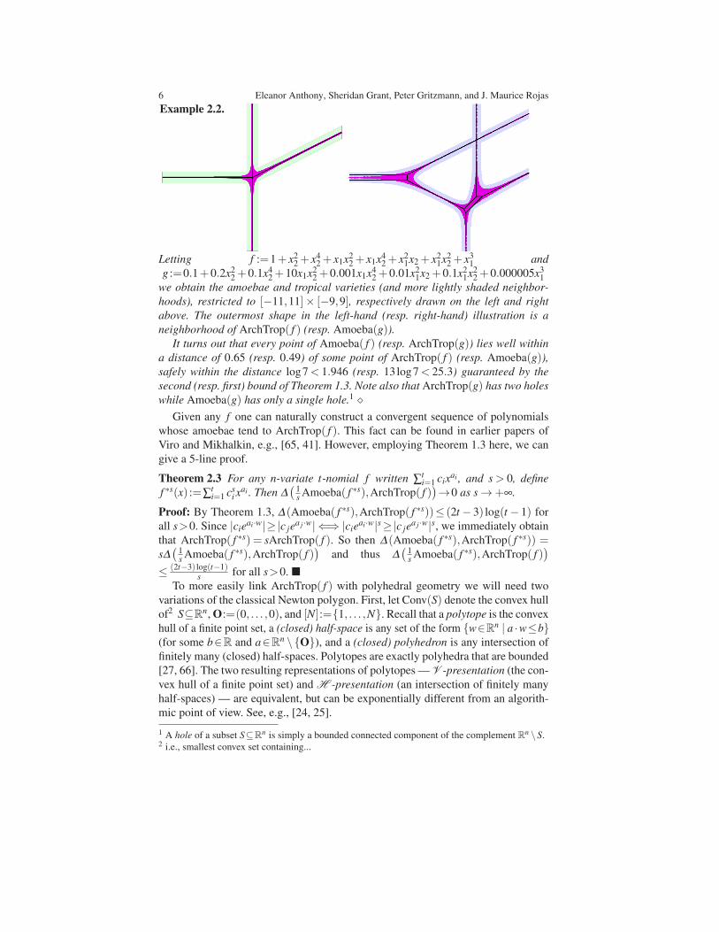
Example 2.2.

Letting f :=1+ x22 + x4

2 + x1x22 + x1x4

2 + x21x2 + x2

1x22 + x3

1 and

g :=0.1+0.2x22 +0.1x4

2 +10x1x22 +0.001x1x4

2 +0.01x21x2 +0.1x2

1x22 +0.000005x3

1

we obtain the amoebae and tropical varieties (and more lightly shaded neighbor-

hoods), restricted to [−11,11]× [−9,9], respectively drawn on the left and right

above. The outermost shape in the left-hand (resp. right-hand) illustration is a

neighborhood of ArchTrop( f ) (resp. Amoeba(g)).It turns out that every point of Amoeba( f ) (resp. ArchTrop(g)) lies well within

a distance of 0.65 (resp. 0.49) of some point of ArchTrop( f ) (resp. Amoeba(g)),safely within the distance log7< 1.946 (resp. 13log7< 25.3) guaranteed by the

second (resp. first) bound of Theorem 1.3. Note also that ArchTrop(g) has two holes

while Amoeba(g) has only a single hole.1 ⋄Given any f one can naturally construct a convergent sequence of polynomials

whose amoebae tend to ArchTrop( f ). This fact can be found in earlier papers of

Viro and Mikhalkin, e.g., [65, 41]. However, employing Theorem 1.3 here, we can

give a 5-line proof.

Theorem 2.3 For any n-variate t-nomial f written ∑ti=1 cix

ai , and s > 0, define

f ∗s(x) :=∑ti=1 cs

i xai . Then ∆

(1sAmoeba( f ∗s),ArchTrop( f )

)→0 as s →+∞.

Proof: By Theorem 1.3, ∆(Amoeba( f ∗s),ArchTrop( f ∗s))≤ (2t − 3) log(t − 1) for

all s>0. Since |cieai·w|≥|c je

a j ·w| ⇐⇒ |cieai·w|s≥|c je

a j ·w|s, we immediately obtain

that ArchTrop( f ∗s) = sArchTrop( f ). So then ∆(Amoeba( f ∗s),ArchTrop( f ∗s)) =s∆


)and thus ∆


)

≤ (2t−3) log(t−1)s

for all s>0. �

To more easily link ArchTrop( f ) with polyhedral geometry we will need two

variations of the classical Newton polygon. First, let Conv(S) denote the convex hull

of2 S⊆Rn, O:=(0, . . . ,0), and [N]:={1, . . . ,N}. Recall that a polytope is the convex

hull of a finite point set, a (closed) half-space is any set of the form {w∈Rn | a ·w≤b}(for some b∈R and a∈Rn \{O}), and a (closed) polyhedron is any intersection of

finitely many (closed) half-spaces. Polytopes are exactly polyhedra that are bounded

[27, 66]. The two resulting representations of polytopes — V -presentation (the con-

vex hull of a finite point set) and H -presentation (an intersection of finitely many

half-spaces) — are equivalent, but can be exponentially different from an algorith-

mic point of view. See, e.g., [24, 25].

1 A hole of a subset S⊆Rn is simply a bounded connected component of the complement Rn \S.2 i.e., smallest convex set containing...


Definition 2.4 Given any n-variate t-nomial f written ∑ti=1 cix

ai , we define its

(ordinary) Newton polytope to be Newt( f ):=Conv({ai}i∈[t]

), and the Archimedean

Newton polytope of f to be ArchNewt( f ) :=Conv({(ai,− log |ci|)}i∈[t]

). Also, for

any polyhedron P ⊂ RN and v ∈ RN , a face of P is any set of the form

Pv := {x∈P | v · x is maximized}. We call v an outer normal of Pv. The dimension

of P, written dimP, is simply the dimension of the smallest affine linear subspace

containing P. Faces of P of dimension 0, 1, and dimP− 1 are respectively called

vertices, edges, and facets. (P and /0 are called improper faces of P, and we set

dim /0 :=−1.) Finally, we call any face of P lower if and only if it has an outer

normal (w1, . . . ,wN) with wN <0, and we let the lower hull of ArchNewt( f ) be the

union of the lower faces of ArchNewt( f ). ⋄

The outer normals of a k-dimensional face of an n-dimensional polyhedron P form

the relative interior of an (n− k)-dimensional polyhedron called an outer normal

cone. Note that ArchNewt( f ) usually has dimension 1 greater than that of Newt( f ).ArchNewt( f ) enables us to relate ArchTrop( f ) to linear optimization.

Proposition 2.5 For any n-variate t-nomial f , ArchTrop( f ) can also be defined

as the set of all w ∈ Rn with maxx∈ArchNewt( f )

{x · (w,−1)} attained on a positive-

dimensional face of ArchNewt( f ).Proof: The quantity |cie

ai·w| attaining its maximum for at least two indices i is

equivalent to the linear form with coefficients (w,−1) attaining its maximimum

for at least two different points in {(ai,− log |ci|)}i∈[t]. Since a face of a polytope is

positive-dimensional if and only if it has at least two vertices, we are done. �

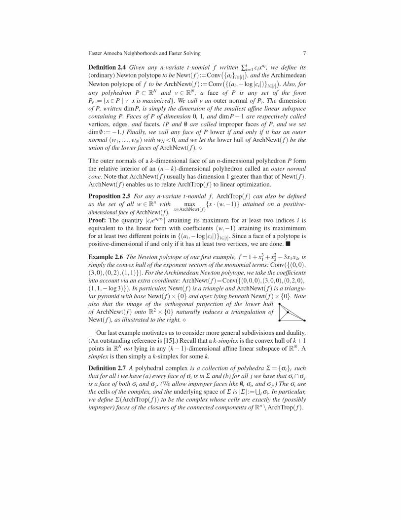
Example 2.6 The Newton polytope of our first example, f =1+ x31 + x2

2 −3x1x2, is

simply the convex hull of the exponent vectors of the monomial terms: Conv({(0,0),(3,0),(0,2),(1,1)}). For the Archimedean Newton polytope, we take the coefficients

into account via an extra coordinate: ArchNewt( f )=Conv({(0,0,0),(3,0,0),(0,2,0),(1,1,− log3)}). In particular, Newt( f ) is a triangle and ArchNewt( f ) is a triangu-

lar pyramid with base Newt( f )×{0} and apex lying beneath Newt( f )×{0}. Note

also that the image of the orthogonal projection of the lower hull

of ArchNewt( f ) onto R2 × {0} naturally induces a triangulation of

Newt( f ), as illustrated to the right. ⋄

Our last example motivates us to consider more general subdivisions and duality.

(An outstanding reference is [15].) Recall that a k-simplex is the convex hull of k+1

points in RN not lying in any (k− 1)-dimensional affine linear subspace of RN . A

simplex is then simply a k-simplex for some k.

Definition 2.7 A polyhedral complex is a collection of polyhedra Σ = {σi}i such

that for all i we have (a) every face of σi is in Σ and (b) for all j we have that σi∩σ j

is a face of both σi and σ j. (We allow improper faces like /0, σi, and σ j.) The σi are

the cells of the complex, and the underlying space of Σ is |Σ | :=⋃i σi. In particular,

we define Σ(ArchTrop( f )) to be the complex whose cells are exactly the (possibly

improper) faces of the closures of the connected components of Rn \ArchTrop( f ).


A polyhedral subdivision of a polyhedron P is then simply a polyhedral complex

Σ ={σi}i with |Σ |=P. We call Σ a triangulation if and only if every σi is a simplex.

Given any finite subset A⊂Rn, a polyhedral subdivision induced by A is then just a

polyhedral subdivision of Conv(A) where the vertices of all the σi lie in A. Finally, the

polyhedral subdivision of Newt( f ) induced by ArchNewt( f ), denoted Σ f , is simply

the polyhedral subdivision whose cells are {π(Q) | Q is a lower face of ArchNewt( f )},

where π : Rn+1 −→ Rn denotes the orthogonal projection forgetting the last coordinate. ⋄Recall that a (polyhedral) cone is just the set of all nonnegative linear combi-

nations of a finite set of points. Such cones are easily seen to always be polyhedra

[27, 66].

Example 2.8 The illustration from Example 2.6 shows a triangulation of the point

set {(0,0),(3,0),(0,2),(1,1)} which happens to be Σ f for f =1+ x31 + x2

2 −3x1x2.

More to the point, it is easily checked that the outer normals to a face of dimension

k of ArchNewt( f ) form a cone of dimension 3−k. In this way, thanks to the natural

partial ordering of cells in any polyhedral complex by inclusion, we get an order-

reversing bijection between the cells of Σ f and pieces of ArchTrop( f ). ⋄That ArchTrop( f ) is always a polyhedral complex follows directly from Proposition

2.5 above. Proposition 2.5 also implies an order-reversing bijection between the

cells Σ f and the cells of Σ(ArchTrop( f )) — an incarnation of polyhedral duality

[66].

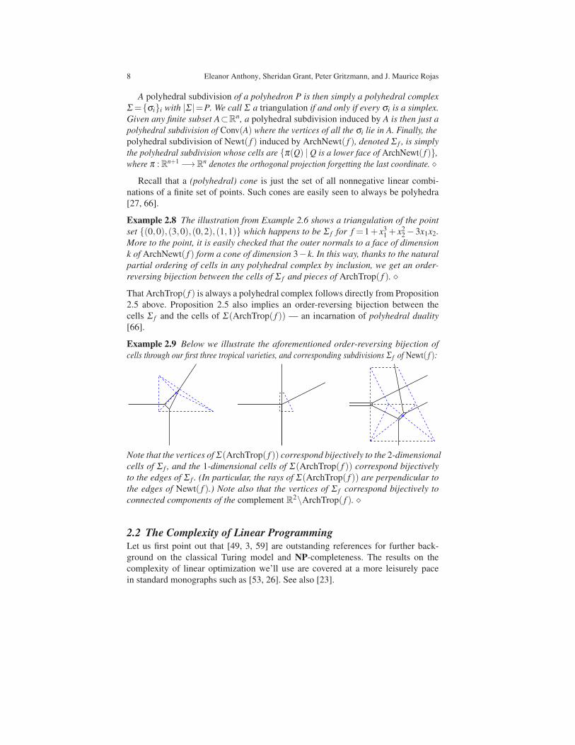
Example 2.9 Below we illustrate the aforementioned order-reversing bijection of

cells through our first three tropical varieties, and corresponding subdivisions Σ f of Newt( f ):

Note that the vertices of Σ(ArchTrop( f )) correspond bijectively to the 2-dimensional

cells of Σ f , and the 1-dimensional cells of Σ(ArchTrop( f )) correspond bijectively

to the edges of Σ f . (In particular, the rays of Σ(ArchTrop( f )) are perpendicular to

the edges of Newt( f ).) Note also that the vertices of Σ f correspond bijectively to

connected components of the complement R2\ArchTrop( f ). ⋄

2.2 The Complexity of Linear ProgrammingLet us first point out that [49, 3, 59] are outstanding references for further back-

ground on the classical Turing model and NP-completeness. The results on the

complexity of linear optimization we’ll use are covered at a more leisurely pace

in standard monographs such as [53, 26]. See also [23].


Definition 2.10 Given any matrix M∈Qk×N with ith row mi, and b:=(b1, . . . ,bk)⊤∈

Qk, the notation Mx≤b means that m1 · x≤b1, . . . ,mk · x≤bk all hold. Given any

c=(c1, . . . ,cN)∈QN we then define the (natural form) linear optimization problem

L (M,b,c) to be the following: Maximize c ·x subject to Mx≤b and x∈RN . We also

define size(L (M,b,c)) := size(M)+ size(b)+ size(c) (see Definition 1.7). The set

of all x∈RN satisfying Mx≤b is the feasible region of L (M,b,c), and when it is

empty we call L (M,b,c) infeasible. Finally, if L (M,b,c) is feasible but does not

admit a well-defined maximum, then we call L (M,b,c) unbounded. ⋄

Theorem 2.11 Given any linear optimization problem L (M,b,c) as defined above,

we can decide infeasibility, unboundedness, or (if L (M,b,c) is feasible, with

bounded maximum) find an optimal solution x∗, all within time polynomial in

size(L (M,b,c)). In particular, if L (M,b,c) is feasible, with bounded maximum,

then we can find an optimal solution x∗ of size polynomial in size(L (M,b,c)). �

Theorem 2.11 goes back to work of Khachiyan in the late 1970s on the Ellipsoid

Method [34], building upon earlier work of Shor, Yudin, and Nemirovskii.

For simplicity, we will not focus on the best current complexity bounds, since

our immediate goal is to efficiently prove polynomiality for our algorithms. We will

need one last complexity result from linear optimization: Recall that a constraint

mi · x≤bi of Mx≤b is called redundant if and only if the corresponding row of M,

and corresponding entry of b, can be deleted from the pair (M,b) without affecting

the feasible region {x∈RN | Mx≤b}.

Lemma 2.12 Given any system of linear inequalities Mx≤b we can, in time poly-

nomial in size(M) + size(b), find a submatrix M′ of M, and a subvector b′ of b,

such that {x∈RN | M′x≤b′}={x∈RN | M′x≤b′} and M′x≤b′ has no redundant

constraints. �

The new set of inequalities M′x ≤ b′ is called an irredundant representation of

Mx≤ b, and can easily be found by solving ≤ k linear optimization problems of

size no larger than size(L (M,b,O)) (see, e.g., [53]).

The linear optimization problems we ultimately solve will have irrational “right-

hand sides”: Our b will usually have entries that are (rational) linear combination

of logarithms of integers. As is well-known in Diophantine Approximation [5], it is

far from trivial to efficiently decide the sign of such irrational numbers. This

problem is equivalent to deciding inequalities of the form αβ11 · · ·αβN

N >1, where the

αi and βi are integers. Note, in particular, that while the number of arithmetic oper-

ations necessary to decide such an inequality is easily seen to be O((∑Ni=1 log |βi|)2)

(via the classical binary method of exponentiation), taking bit-operations into

account naively results in a problem that appears to have complexity exponential in

log |β1|+ · · ·+ log |βN |. But we can in fact go much faster...

2.3 Irrational Linear Optimization and Approximating LogarithmsRecall the following result on comparing monomials in rational numbers.


Theorem 2.13 [11, Sec. 2.4] Suppose α1, . . . ,αk ∈Q are positive and β1, . . . ,βk ∈Z. Also let A be the maximum of the numerators and denominators of the αi (when

written in lowest terms) and B :=maxi{|βi|}. Then, within

O(k30k log(B)(log logB)2 log loglog(B)(log(A)(log logA)2 log log logA)k

)

bit operations, we can determine the sign of αβ11 · · ·αβk

k −1. �

While the underlying algorithm is a simple application of Arithmetic-Geometric

Mean Iteration (see, e.g., [9]), its complexity bound hinges on a deep estimate of

Nesterenko [43], which in turn refines seminal work of Matveev [40] and Alan

Baker [5] on linear forms in logarithms.

Definition 2.14 We call a polyhedron P ℓ-rational if and only if it is of the form

{x∈Rn | Mx≤b} with M∈Qk×n and b=(b1, . . . ,bk)⊤ satisfying

bi=β1,i log |α1|+ · · ·+βk,i log |αk|,with βi, j,α j ∈Q for all i and j. Finally, we set

size(P) :=size(M)+ size([βi, j])+∑ki=1 size(αi). ⋄

Via the Simplex Method (or even a brute force search through all n-tuples of

facets of P) we can obtain the following consequence of Theorems 2.11 and 2.13.

Corollary 2.15 Following the notation of Definition 2.14, suppose n is fixed. Then

we can decide whether P is empty, compute an irredundant representation for P, and

enumerate all maximal sets of facets determining vertices of P, in time polynomial

in size(P). �

The key trick behind the proof of Corollary 2.15 is that the intermediate linear op-

timization problems needed to find an irredundant representation for P use linear

combinations (of rows of the original representation) with coefficients of moderate

size (see, e.g., [53]).

3 Tropical Start-Points for Numerical Iteration and an Example

We begin by outlining a method for picking start-points for Newton Iteration

(see, e.g., [12, Ch. 8] for a modern perspective) and Homotopy Continuation

[31, 62, 64, 37, 7]. While we do not discuss these methods for solving polyno-

mial equations in further detail, let us at least point out that Homotopy Continua-

tion (combined with Smale’s α-Theory for certifying roots [12, 7]) is currently the

fastest, most easily parallelizable, and reliable method for numerically solving poly-

nomial systems in complete generality. Other important methods include Resultants

[18] and Grobner Bases [20]. While these alternative methods are of great utility

in certain algebraic and theoretical applications [1, 19], Homotopy Continuation is

currently the method of choice for practical numerical computation with extremely

large polynomial systems.

Algorithm 3.1 (Coarse Approximation to Roots with Log-Norm Vector Near a

Given Query Point)

INPUT. Polynomials f1, . . . , fn∈Q[√

−1][

x±11 , . . . ,x±1

n

], with fi(x)=∑

tij=1 ci, jx

a j(i)

an n-variate ti-nomial for all i, and a query point w∈Qn.


OUTPUT. An ordered n-tuple of sets of indices (Ji)ni=1 such that, for all i,

gi :=∑ j∈Jici, jx

a j(i) is a sub-summand of fi, and the roots

of G :=(g1, . . . ,gn) are approximations of the roots of

F :=( f1, . . . , fn) with log-norm vector nearest w.

DESCRIPTION.

1. Let σw be the closure of the unique cell of Σ(⋃n

i=1 ArchTrop( fi)) (see Definition

2.7) containing w.

2. If σw has no vertices in⋂n

i=1 ArchTrop( fi) then output an irredundant collection

of facet inequalities for σw, output ‘‘There are no roots of F in

σw.’’, and STOP.

3. Otherwise, fix any vertex v of σw ∩⋂ni=1 ArchTrop( fi) and, for each i∈ [n], let

Ei be any edge of ArchNewt( fi) generating a facet of ArchTrop( fi) containing v.

4. For all i∈ [n], let Ji :={ j | (a j(i),− log |ci, j|)∈Ei}.

5. Output (Ji)ni=1. �

Thanks to our main results and our preceding observations on linear optimization,

we can easily obtain that our preceding algorithm has complexity polynomial in

size(F) for fixed n. In particular, Step 1 is (resp. Steps 2 and 3 are) accomplished

via the algorithm underlying Theorem 1.5 (resp. Corollary 2.15).

The key subtlety then is to prove that, for most inputs, our algorithm actually

gives useful approximations to the roots with log-norm vector nearest the input

query point w, or truthfully states that there are no root log-norm vectors in σw.

We leave the precise metric estimates defining “most inputs” for future work.

However, we point out that a key ingredient is the A -discriminant [22], and a

recent polyhedral approximation of its amoeba [50] refining the tropical

discriminant [16]. So we will now clarify the meaning of the output of our algorithm.

The output system G is useful because, with high probability (in the sense of

random liftings, as in [18, Lemma 6.2]), all the gi are binomials, and binomial

systems are particularly easy to solve: They are equivalent to linear equations in

the logarithms of the original variables. In particular, any n× n binomial system

always has a unique vector of norms for its roots.

Recall the standard notation Jac(F) :=[

∂ fi∂x j

]n×n

. The connection to Newton

Iteration is then easy to state: Use any root of G as a start-point z(0) for the iteration

z(n+1) :=z(n)− Jac(F)−1|z(n)F(z(n)). The connection to Homotopy Continuation

is also simple: Use the pair (G,ζ ) (for any root ζ of G) to start a path converging

(under the usual numerical conditioning assumptions on whatever predictor-corrector

method one is using) to a root of F with log-norm vector near w. Note also that while

it is safer to do the extra work of Homotopy Continuation, there will be cases where

the tropical start-points from Algorithm 3.1 are sufficiently good for mere Newton

Iteration to converge quickly to a true root.

Remark 3.2 Note that, when applying Algorithm 3.1 for later Homotopy

Continuation, we have the freedom to follow as few start-points, or as few paths,

as we want. When our start-points (resp. paths) indeed converge to nearby roots, we

obtain a tremendous savings over having to follow all start-points (resp. paths). ⋄


Definition 3.3 Given any n-dimensional polyhedra P1, . . . ,Pn⊂Rn, we call a vertex

v of⋂n

i=1 Pi mixed if and only if v lies on a facet of Pi for all i. ⋄

Note that, by construction, any vertex chosen in Step 3 of Algorithm 3.1 is mixed.

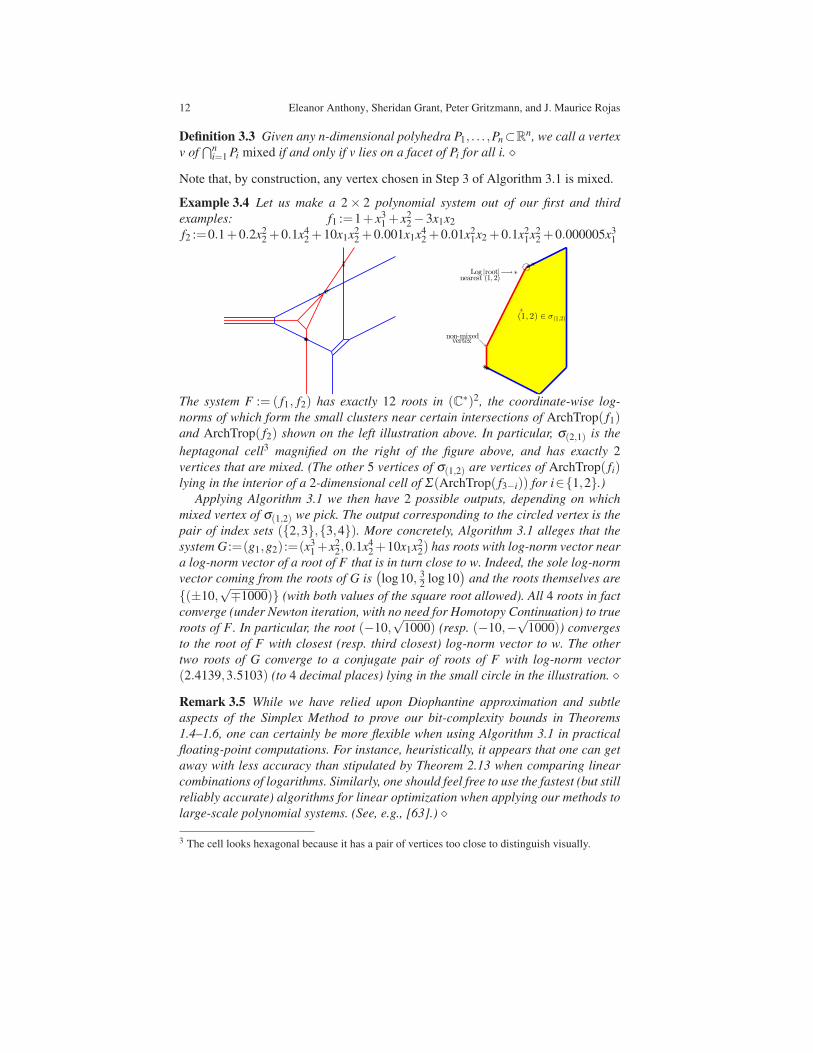
Example 3.4 Let us make a 2 × 2 polynomial system out of our first and third

examples: f1 :=1+ x31 + x2

2 −3x1x2

f2 :=0.1+0.2x22 +0.1x4

2 +10x1x22 +0.001x1x4

2 +0.01x21x2 +0.1x2

1x22 +0.000005x3

1

(1, 2) ∈ σ(1,2)

Log |root|−→nearest (1, 2)

non-mixedցvertex

The system F := ( f1, f2) has exactly 12 roots in (C∗)2, the coordinate-wise log-

norms of which form the small clusters near certain intersections of ArchTrop( f1)and ArchTrop( f2) shown on the left illustration above. In particular, σ(2,1) is the

heptagonal cell3 magnified on the right of the figure above, and has exactly 2

vertices that are mixed. (The other 5 vertices of σ(1,2) are vertices of ArchTrop( fi)lying in the interior of a 2-dimensional cell of Σ(ArchTrop( f3−i)) for i∈{1,2}.)

Applying Algorithm 3.1 we then have 2 possible outputs, depending on which

mixed vertex of σ(1,2) we pick. The output corresponding to the circled vertex is the

pair of index sets ({2,3},{3,4}). More concretely, Algorithm 3.1 alleges that the

system G:=(g1,g2):=(x31+x2

2,0.1x42+10x1x2

2) has roots with log-norm vector near

a log-norm vector of a root of F that is in turn close to w. Indeed, the sole log-norm

vector coming from the roots of G is(log10, 3

2log10

)and the roots themselves are

{(±10,√∓1000)} (with both values of the square root allowed). All 4 roots in fact

converge (under Newton iteration, with no need for Homotopy Continuation) to true

roots of F. In particular, the root (−10,√

1000) (resp. (−10,−√

1000)) converges

to the root of F with closest (resp. third closest) log-norm vector to w. The other

two roots of G converge to a conjugate pair of roots of F with log-norm vector

(2.4139,3.5103) (to 4 decimal places) lying in the small circle in the illustration. ⋄

Remark 3.5 While we have relied upon Diophantine approximation and subtle

aspects of the Simplex Method to prove our bit-complexity bounds in Theorems

1.4–1.6, one can certainly be more flexible when using Algorithm 3.1 in practical

floating-point computations. For instance, heuristically, it appears that one can get

away with less accuracy than stipulated by Theorem 2.13 when comparing linear

combinations of logarithms. Similarly, one should feel free to use the fastest (but still

reliably accurate) algorithms for linear optimization when applying our methods to

large-scale polynomial systems. (See, e.g., [63].) ⋄

3 The cell looks hexagonal because it has a pair of vertices too close to distinguish visually.


4 Proof of Theorem 1.5

Using t − 1 comparisons, we can isolate all indices i such that maxi |cieai·w| is

attained. Thanks to Theorem 2.13 this can be done in polynomial-time. We then

obtain, say, J equations of the form ai ·w=− log |ci| and K inequalities of the form

ai ·w>− log |ci| or ai ·w<− log |ci|.Thanks to Lemma 2.12, combined with Corollary 2.15, we can determine the

exact cell of ArchTrop( f ) containing w if J ≥ 2. Otherwise, we obtain the unique

cell of Rn\ArchTrop( f ) with relative interior containing w. Note also that an (n−1)-dimensional face of either kind of cell must be the dual of an edge of ArchNewt( f ).Since every edge has exactly 2 vertices, there are at most t(t − 1)/2 such (n− 1)-dimensional faces, and thus σw is the intersection of at most t(t −1)/2 half-spaces.

So we are done. �

Remark 4.1 Theorem 1.5 also generalizes an earlier complexity bound from [4]

for deciding membership in ArchTrop( f ). ⋄

5 Proof of Theorem 1.4

Note The hurried reader will more quickly grasp the following proof after briefly

reviewing Theorems 1.3, 1.5, and 2.13.

Since ArchTrop( f ) and Amoeba( f ) are closed and non-empty, infv∈ArchTrop( f ) |v−w|= |w− v′| for some point v′ ∈ArchTrop( f ) and infu∈Amoeba( f ) |u−w|= |w− u′|for some point u′∈Amoeba( f ).

Now, by the second upper bound of Theorem 1.3, there is a point v′′∈ArchTrop( f )within distance log(t − 1) of u′. Clearly, |w− v′|≤ |w− v′′|. Also, by the Triangle

Inequality, |w− v′′|≤|w−u′|+ |u′− v′′|. So then,

infv∈ArchTrop( f ) |v−w|≤ infu∈Amoeba( f ) |u−w|+ log(t −1),and thus infu∈Amoeba( f ) |u−w|− infv∈ArchTrop( f ) |v−w|≥− log(t −1).

Similarly, by the first upper bound of Theorem 1.3, there is a point u′′∈Amoeba( f )within distance (2t − 3) log(t − 1) of v′. Clearly, |w− u′| ≤ |w− u′′|. Also, by the

Triangle Inequality, |w− u′′|≤ |w− v′|+ |v′− u′′|. So then, infu∈Amoeba( f ) |u−w|≤infv∈ArchTrop( f ) |v−w|+(2t −3) log(t −1), and thus

infu∈Amoeba( f ) |u−w|− infv∈ArchTrop( f ) |v−w|≤(2t −3) log(t −1).So our first assertion is proved.

Now if f has coefficients with real and imaginary parts that are rational, and n is

fixed, Theorem 1.5 (which we’ve already proved) tells us that we can decide whether

w lies in ArchTrop( f ) using a number of bit operations polynomial in size(w) +size( f ). So we may assume w 6∈ArchTrop( f ) and dimσw=n.

Theorem 1.5 also gives us an explicit description of σw as the intersection of a

number of half-spaces polynomial in t. Moreover, σw is ℓ-rational (recall Definition

2.14), with size polynomial in size( f ). So we can compute the distance D from w to

ArchTrop( f ) by finding which facet of σw has minimal distance to w. The distance

from w to any such facet can be approximated to the necessary number of bits in

polynomial-time via Theorem 2.13 and the classical formula for distance between

a point and an affine hyperplane: infu∈{x | r·x=s} |u−w| = (|r ·w|− sign(r ·w)s)/|r|.More precisely, comparing the facet distances reduces to checking the sign of an


expression of the form γ1 + γ2 log(

cici′

)+ γ3 log

(c j

c j′

)where γ1 (resp. γ2, γ3) is a

rational linear combination of√

|ai −ai′ | and√

|a j −a j′ | (resp. rational multiple

of√|ai −ai′ | or

√|a j −a j′ |), with coefficients of size polynomial in size( f ), for

some indices i, i′, j, j′∈ [t]. We can then efficiently approximate D by approximat-

ing the underlying square-roots and logarithms to sufficient precision. The latter

can be accomplished by Arithmetic-Geometric Iteration, as detailed in [9], and the

amount of precision needed is explicitly bounded by an earlier variant of Theo-

rem 2.13 covering inhomogeneous linear combinations of logarithms of algebraic

numbers with algebraic coefficients [5]. The resulting bounds are somewhat worse

than in Theorem 2.13, but still allow us to find polynomially many leading bits of

infv∈Amoeba( f ) |v−w| (for w∈Qn) in time polynomial in size(w)+ size( f ).To prove the final assertion, we merely decide whether infv∈ArchTrop( f ) |v−w|

strictly exceeds log(t − 1) or not. To do so, we need only compute a polynomial

number of leading bits of infv∈ArchTrop( f ) |v−w| (thanks to Theorem 2.13), and this

takes time polynomial in size(w)+ size( f ). Thanks to our initial observations using

the Triangle Inequality, it is clear that Output (b) or Output (a) occurs according as

infv∈ArchTrop( f ) |v−w|> log(t −1) or not. So we are done. �

6 Proving Theorem 1.6

6.1 Fast Cell Computation: Proof of the First Assertion

First, we apply Theorem 1.5 to ( fi,w) for each i∈ [k] to find which ArchTrop( fi)contain w.

If w lies in no ArchTrop( fi), then we simply use Corollary 2.15 (as in our

proof of Theorem 1.5) to find an explicit description of the closure of the cell of

Rn\⋃ki=1 ArchTrop( fi) containing w. Otherwise, we find the cells of ArchTrop( fi)

(for those i with ArchTrop( fi) containing w) that contain w. Then, applying Corol-

lary 2.15 once again, we explicitly find the unique cell of⋂

ArchTrop( fi)∋w

ArchTrop( fi)containing w.

Assume that fi has exactly ti monomial terms for all i. In either of the preceding

cases, the total number of half-spaces involved is no more than ∑ki=1 ti(ti −1)/2. So

the overall complexity of our redundancy computations is polynomial in the input

size and we are done. �

6.2 Hardness of Detecting Mixed Vertices: Proving the Second

Assertion

It will clarify matters if we consider a related NP-hard problem for rational poly-

topes first.

Ultimately, our proof boils down to a reduction from the following problem,

equivalent to the famous NP-complete PARTITION problem (see below): Decide if

a vertex of the hypercube [−1,1]n lies on a prescribed hyperplane defined by an

equation of the form a · x=0 with a∈Zn. Because the coordinates of a are integral,


we can replace the preceding equation by the inequality 0≤a · x≤1/2. With a bit

more work, we can reduce PARTITION to the detection of a mixed vertex for a

particular intersection of polyhedra. We now go over the details.

6.2.1 Preparation over Q

In the notation of Definition 3.3, let us first consider the following decision problem.

We assume all polyhedra are given explicitly as finite collections of rational linear

inequalities, with size defined as in Section 2.2.

MIXED-VERTEX:

Given n ∈ N and polyhedra P1, . . . ,Pn in Rn, does P :=⋂n

i=1 Pi have a mixed vertex? �

While MIXED-VERTEX can be solved in polynomial time when n is fixed (by a

brute-force check over all mixed n-tuples of facets), we will show that, for n varying,

the problem is NP-complete, even when restricting to the case where all polytopes

are full-dimensional and P1, . . . ,Pn−1 are axes-parallel bricks.

Let ei denote the ith standard basis vector in Rn and let M⊤ denote the transpose

of a matrix M. Also, given α ∈ Rn and b ∈ R, we will use the following

notation for hyperplanes and certain half-spaces in Rn determined by α and b:

H(α ,b) := {x ∈ Rn | α · x = b}, H≤(α ,b)

:= {x ∈ Rn | α · x ≤ b}. For i∈ [n], let si ∈N,

Mi := [mi,1, . . . ,mi,si]⊤ ∈ Zsi×n, bi := (bi,1, . . . ,bi,si

)⊤ ∈ Zsi , and

Pi := {x ∈ Rn | Mix ≤ bi}. Since linear optimization can be done in polynomial-

time (in the cases we consider) we may assume that the presentations (n,si;Mi,bi)are irredundant, i.e., Pi has exactly si facets if Pi is full-dimensional, and the sets

Pi ∩H(mi, j ,bi, j), for j∈ [si], are precisely the facets of Pi for all i∈ [n].

Now set P :=⋂n

i=1 Pi. Note that size(P) is thus linear in ∑ni=1 size(Pi).

Lemma 6.1 MIXED-VERTEX ∈ NP.

Proof: Since the binary sizes of the coordinates of the vertices of P are bounded

by a polynomial in the input size, we can use vectors v ∈ Qn of polynomial size as

certificates. We can check in polynomial-time whether such a vector v is a vertex of

P. If this is not the case, v cannot be a mixed vertex of P. Otherwise, v is a mixed

vertex of P if and only if for each i∈ [n] there exists a facet Fi of Pi with v∈Fi. Since

the facets of the polyhedra Pi admit polynomial-time decriptions as H -polyhedra,

this can be checked by a total of s1 + · · ·+ sn polyhedral membership tests. These

membership tests are easily doable in polynomial-time since any of the underlying

inequalities can be checked in polynomial-time and the number of faces of any Pi

no worse than linear in the size of Pi.

So we can check in polynomial-time whether a given certificate v is a mixed

vertex of P. Hence MIXED-VERTEX is in NP. �

Since (in fixed dimension) we can actually list all vertices of P in polynomial-

time, it is clear that MIXED-VERTEX can be solved in polynomial-time when n is

fixed. When n is allowed to vary we obtain hardness:

Theorem 6.2 MIXED-VERTEX is NP-hard, even in the special case where P1, . . . ,Pn−1

are centrally symmetric axes-parallel bricks with vertex coordinates in {±1,±2},


and Pn has at most 2n+ 2 facets (with 2n of them parallel to coordinate hyper-

planes).

The proof of Theorem 6.2 will be based on a reduction from the following deci-

sion problem:

PARTITION

Given d,α1, . . . ,αd ∈ N, is there an I⊆ [d] such that ∑i∈I αi = ∑i∈[d]\I αi? �

PARTITION was in the original list of NP-complete problems from [33].

Let an instance (d;α1, . . . ,αd) of PARTITION be given, and set α := (α1, . . . ,αd).Then we are looking for a point x ∈ {−1,1}d with α · x = 0.

We will now construct an equivalent instance of MIXED-VERTEX. With n :=d +1, x := (x1, . . . ,xn−1) and 11n := (1, . . . ,1) ∈ Rn let

Pi :={(x,xn)|−1 ≤ xi ≤ 1,−2 ≤ x j ≤ 2 for all j ∈ [n]\{i}

}.

Also, for i ∈ [n−1], let

Pn := { (x,xn) | −2 ·11n−1 ≤ x ≤ 2 ·11n−1,−1 ≤ xn ≤ 1, 0 ≤ 2α · x ≤ 1}and set P :=

⋂ni=1 Pi, α := (α,0).

The next lemma shows that Pn ∩{−1,1}n still captures the solutions of the given

instance of partition.

Lemma 6.3 (d;α1, . . . ,αd) is a “no”-instance of PARTITION if and only if Pn ∩{−1,1}n is empty.

Proof: Suppose, first, that (d;α1, . . . ,αd) is a “no”-instance of PARTITION. If Pn

is empty there is nothing left to prove. So, let y ∈ Pn and w ∈ {−1,1}n−1 ×R.

Since α ∈ Nd we have |α ·w| ≥ 1. Hence, via the Cauchy-Schwarz inequality, we

have 1 ≤ |α ·w| = |α · y+ α · (w− y)| ≤ |α · y|+ |α · (w− y)| ≤ 12+ |α| · |w− y| =

12+ |α| · |w− y| and thus |w− y| ≥ 1

2|α| > 0. Therefore Pn ∩({−1,1}n−1 ×R

)is

empty.

Conversely, if Pn ∩ {−1,1}n is empty, then there is no x∈ {±1}n−1 such that

0≤α · x≤ 12. Since α ∈Nn−1, we have that (d,α1, . . . ,αd) is a “No”-instance of

PARTITION. �

The next lemma reduces the possible mixed vertices to the vertical edges of the

standard cube.

Lemma 6.4 Following the preceding notation, let v be a mixed vertex of P :=⋂ni=1 Pi. Then v∈{−1,1}n−1 × [−1,1].

Proof: First note that Q :=⋂n−1

i=1 Pi = [−1,1]n−1 × [−2,2]. Therefore, for each i∈[n− 1], the only facets of Pi that meet Q are those in H(ei,±1) and H(en,±2). Since

P ⊂ [−1,1]n, and for each i ∈ [n−1] the mixed vertex v must be contained in a facet

of Pi, we have v ∈ [−1,1]n ∩n−1⋂

i=1

⋃

δi∈{−1,1}H(ei,δi)

= {−1,1}n−1 × [−1,1], which

proves the assertion. �

The next lemma adds Pn to consideration.


Lemma 6.5 Let v be a mixed vertex of P :=⋂n

i=1 Pi. Then v∈{−1,1}n.

Proof: By Lemma 6.4, v∈{−1,1}n−1 × [−1,1]. Since the hyperplanes H(ei,±2) do

not meet [−1,1]n, we have v 6∈ H(ei,−2)∪H(ei,2) for all i∈ [n−1]. Hence, v can only

be contained in the constraint hyperplanes H(α,0),H(2α,1),H(en,−1),H(en,1). Since α ∈Rn−1×{0}, the vector α is linearly dependent on e1, . . . ,en−1. Hence, v∈H(en,−1)∪H(en,1), i.e., v ∈ {−1,1}n. �

We can now prove the NP-hardness of MIXED-VERTEX.

Proof of Theorem 6.2: First, let (d;α1, . . . ,αd) be a “yes”-instance of PARTITION,

let x∗ := (ξ ∗1 , . . . ,ξ

∗n−1)∈{−1,1}n−1 be a solution, and set ξ ∗

n := 1, v :=(x∗,ξ ∗n ),

Fi :=H(ei,ξ∗i )∩Pi for all i∈ [n], and Fn :=H(α,0)∩Pn. Then v ∈ Fn ⊂ Pn, hence v ∈ P

and, in fact, v is a vertex of P. Furthermore, Fi is a facet of Pi for all i∈[n], v∈⋂ni=1 Fi,

and thus v is a mixed vertex of P.

Conversely, let (d;α1, . . . ,αd) be a “no”-instance of PARTITION, and suppose

that v ∈ Rn is a mixed vertex of P. By Lemma 6.5, v∈{−1,1}n. Furthermore, v

lies in a facet of Pn. Hence, in particular, v ∈ Pn, i.e., Pn ∩{−1,1}n is non-empty.

Therefore, by Lemma 6.3, (d;α1, . . . ,αd) is a “yes”-instance of PARTITION. This

contradiction shows that P does not have a mixed vertex.

Clearly, the transformation works in polynomial-time. �

6.3 Proof of the Second Assertion of Theorem 1.6It clearly suffices to show that the following variant of MIXED-VERTEX is NP-hard:

LOGARITHMIC-MIXED-VERTEX:

Given n ∈ N and ℓ-rational polyhedra P1, . . . ,Pn ⊂Rn, does P :=⋂n

i=1 Pi have a

mixed vertex? �

Via an argument completely parallel to the last section, the NP-hardness of

LOGARITHMIC-MIXED-VERTEX follows immediately from the NP-hardness of

the following variant of PARTITION:

LOGARITHMIC-PARTITION

Given d ∈ N, α1, . . . ,αd ∈ N \ {0}, is there an I ⊆ [d] such that ∑i∈I logαi =

∑i∈[d]\I logαi? �

We measure size in LOGARITHMIC-PARTITION just as in the original

PARTITION Problem: ∑di=1 logαd . Note that LOGARITHMIC-PARTITION is equiv-

alent to the obvious variant of PARTITION where we ask for a partition making the

two resulting products be identical. The latter problem is known to be NP-hard as

well, thanks to [45], and is in fact also strongly NP-hard. �

References1. D’Andrea, Carlos; Krick, Teresa; Sombra, Martin, “Heights of varieties in multiprojective

spaces and arithmetic Nullstellensatze,” Annales Scientifiques de l’ENS, fascicule 4 (2013),

pp. 549–627.

2. D’Andrea, Carlos; Galligo, Andre; and Sombra, Martin, “Quantitative Equidistribution for the

Solution of a System of Sparse Polynomial Equations,” American Journal of Mathematics, to

appear.


3. Arora, Sanjeev and Barak, Boaz, Computational complexity. A modern approach. Cambridge

University Press, Cambridge, 2009.

4. Avendano, Martın; Kogan, Roman; Nisse, Mounir; and Rojas, J. Maurice, “Metric Estimates

and Membership Complexity for Archimedean Amoebae and Tropical Hypersurfaces,” submit-

ted for publication, also available as Math ArXiV preprint 1307.3681

5. Baker, Alan, “The theory of linear forms in logarithms,” in Transcendence Theory: Advances

and Applications: proceedings of a conference held at the University of Cambridge, Cam-

bridge, Jan.–Feb., 1976, Academic Press, London, 1977.

6. Baker, Matthew and Rumely, Robert, Potential theory and dynamics on the Berkovich pro-

jective line,” Mathematical Surveys and Monographs, 159, American Mathematical Society,

Providence, RI, 2010.

7. Bates, Daniel J.; Hauenstein, Jonathan D.; Sommese, Andrew J.; and Wampler, Charles W.,

Numerically Solving Polynomial Systems with Bertini, Software, Environments and Tools

series, Society for Industrial and Applied Mathematics, 2013.

8. Beltran, Carlos and Pardo, Luis M., “Smale’s 17th Problem: Average Polynomial Time to com-

pute affine and projective solutions,” Journal of the American Mathematical Society, 22 (2009),

pp. 363–385.

9. Bernstein, Daniel J., “Computing Logarithm Intervals with the Arithmetic-Geometric Mean

Iterations,” available from http://cr.yp.to/papers.html .

10. Bettale, Luk; Faugere, Jean-Charles; and Perret, Ludovic, “Cryptanalysis of HFE, multi-HFE

and variants for odd and even characteristic,” Designs, Codes and Cryptography, Oct. 2013,

vol. 69, issue 1, pp. 1–52.

11. Bihan, Frederic; Rojas, J. Maurice; and Stella, Casey, “Faster Real Feasibility via Circuit

Discriminants,” proceedings of ISSAC 2009 (July 28–31, Seoul, Korea), pp. 39–46, ACM

Press, 2009.

12. Blum, Lenore; Cucker, Felipe; Shub, Mike; and Smale, Steve, Complexity and Real Compu-

tation, Springer-Verlag, 1998.

13. Burgisser, Peter and Scheiblechner, Peter, “On the Complexity of Counting Components of

Algebraic Varieties,” Journal of Symbolic Computation 44(9), pp. 1114–1136, 2009.

14. Burgisser, Peter and Cucker, Felipe, “Solving Polynomial Equations in Smoothed Polynomial

Time and a Near Solution to Smale’s 17th Problem,” Proceedings STOC (Symposium on the

the Theory of Computation) 2010, pp. 503-512, ACM Press, 2010.

15. De Loera, Jesus A.; Rambau, Jorg; Santos, Francisco, Triangulations, Structures for algo-

rithms and applications, Algorithms and Computation in Mathematics, 25, Springer-Verlag,

Berlin, 2010.

16. Dickenstein, Alicia; Feichtner, Eva Maria; Sturmfels, Bernd, “Tropical discriminants,” J.

Amer. Math. Soc. 20 (2007), no. 4, pp. 1111–1133.

17. Einsiedler, Manfred; Kapranov, Mikhail; and Lind, Douglas, “Non-archimedean amoebas and

tropical varieties,” Journal fur die reine und angewandte Mathematik (Crelles Journal), Vol.

2006, no. 601, pp. 139–157, 2006.

18. Emiris, Ioannis Z. and Canny, John, “Efficient Incremental Algorithms for the Sparse Resul-

tant and Mixed Volume,” J. Symbolic Comput. 20 (1995), no. 2, pp. 117–149.

19. Faugere, Jean-Charles; Gaudry, Pierrick; Huot, Louise; and Renault, Guenael, “Using Sym-

metries in the Index Calculus for Elliptic Curves Discrete Logarithm,” Journal of Cryptology,

pp. 1–40, 2013.

20. Faugere, Jean-Charles; Hering, Milena; and Phan, Jeffrey, “The membrane inclusions curva-

ture equations,” Advances in Applied Mathematics, 31(4):643-658, June 2003.

21. Garey, Michael R. and Johnson, David S., Computers and Intractability: A Guide to the Theory

of NP-Completeness, A Series of Books in the Mathematical Sciences, W. H. Freeman and Co.,

San Francisco, Calif., 1979.

22. Gel’fand, Israel Moseyevitch; Kapranov, Misha M.; and Zelevinsky, Andrei V.; Discriminants,

Resultants and Multidimensional Determinants, Birkhauser, Boston, 1994.

23. Gritzmann, Peter, Grundlagen der Mathematischen Optimierung: Diskrete Strukturen, Kom-

plexitatstheorie, Konvexitatstheorie, Lineare Optimierung, Simplex-Algorithmus, Dualitat,

Springer Vieweg, 2013.


24. Gritzmann, Peter and Klee, Victor, “On the complexity of some basic problems in computa-

tional convexity: I. Containment problems,” Discrete Math. 136 (1994), pp. 129–174.

25. Gritzmann, Peter and Klee, Victor, “On the complexity of some basic problems in computa-

tional convexity: II. Volume and mixed volumes,” in Polytopes: Abstract, Convex and Compu-

tational (Ed. by T. Bisztriczky, P. McMullen, R. Schneider, and A. Ivic Weiss); Kluwer, Boston

1994, pp. 373–466.

26. Grotschel, Martin; Lovasz, Laszlo; and Schrijver, Alexander, Geometric Algorithms and Com-

binatorial Optimization, Springer-Verlag, New York, 1993.

27. Grunbaum, Branko, Convex Polytopes, Wiley-Interscience, London, 1967; 2nd ed. (edited by

Ziegler, G.), Graduate Texts in Mathematics, vol. 221, Springer-Verlag, 2003.

28. Hao, Wenrui; Hauenstein, Jonathan D.; Hu, Bei; Liu, Yuan; Sommese, Andrew; and Zhang,

Yong-Tao, “Continuation Along Bifurcation Branches for a Tumor Model with a Necrotic

Core,” Journal of Scientific Computation, 53:395–413, 2012.

29. Hauenstein, Jonathan; Rodriguez, Jose; and Sturmfels, Bernd, “Maximum likelihood for ma-

trices with rank constraints,” Journal of Algebraic Statistics, to appear. Also available as Math

ArXiV preprint 1210.0198 .

30. Herbst, Manfred; Hori, Kentaro; and Page, David, “Phases of N=2 theories in 1+1 dimen-

sions with boundary,” High Energy Physics ArXiV preprint 0803.2045v1 .

31. Huan, Liang Jiao and Li, Tien-Yien, “Parallel homotopy algorithm for symmetric large sparse

eigenproblems,” Journal of Computational and Applied Mathematics, Volume 60, Issues 1–2,

20 June 1995, pp. 77–100.

32. Itenberg, Ilia; Mikhalkin, Grigory; and Shustin, Eugenii, Tropical algebraic geometry, Second

edition, Oberwolfach Seminars, 35, Birkhauser Verlag, Basel, 2009.

33. Karp, Richard M., “Reducibility among combinatorial problems,” in Complexity of Computer

Computations, (Miller, R. E. and Thatcher, J. W., eds.), Plenum Press, New York, pp. 85–103,

1972.

34. Khachiyan, Leonid, “A polynomial algorithm in linear programming,” Soviet Math. Doklady

20, pp. 191–194, 1979.

35. Khovanskii, Askold G., Fewnomials, AMS Press, Providence, Rhode Island, 1991.

36. Koiran, Pascal; Portier, Natacha; and Rojas, J. Maurice, “Counting Tropically Degenerate Val-

uations and p-adic Approaches to the Hardness of the Permanent,” submitted for publication,

also available as Math ArXiV preprint 1309.0486 .

37. Lee, Tsung-Lin and Li, Tien-Yien, “Mixed volume computation in solving polynomial sys-

tems,” in Randomization, Relaxation, and Complexity in Polynomial Equation Solving, Con-

temporary Mathematics, vol. 556, pp. 97–112, AMS Press, 2011.

38. Tropical and Idempotent Mathematics, International Workshop TROPICAL-07 (Tropical and

Idempotent Mathematics, Aug. 25—30, 2007, Independent University, edited by G. L. Litvinov

and S. N. Sergeev), Contemporary Mathematics, vol. 495, AMS Press, 2009.

39. Maclagan, Diane and Sturmfels, Bernd, Introduction to Tropical Geometry, in progress, 2014.

40. Matveev, Eugene M., “An explicit lower bound for a homogeneous rational linear form in

logarithms of algebraic numbers. II.” Izv. Ross. Akad. Nauk Ser. Mat. 64 (2000), no. 6, pp.

125–180; translation in Izv. Math. 64 (2000), no. 6, pp. 1217–1269.

41. Mikhalkin, Grigory, “Decomposition into pairs-of-pants for complex algebraic hypersur-

faces,” Topology , vol. 43, no. 5, pp. 1035–1065, 2004.

42. Muller, Stefan; Feliu, Elisenda; Regensburger, Georg; Conradi, Carsten; Shiu, Anne; and

Dickenstein, Alicia, “Sign conditions for injectivity of generalized polynomial maps with ap-

plications to chemical reaction networks and real algebraic geometry,” Math ArXiV preprint

1311.5493 .

43. Nesterenko, Yuri, “Linear forms in logarithms of rational numbers,” Diophantine approxima-

tion (Cetraro, 2000), pp. 53–106, Lecture Notes in Math., 1819, Springer, Berlin, 2003.

44. Newton, Isaac, Letter to Oldenburg dated 1676 Oct 24, the correspondence of Isaac Newton,

II, pp. 126–127, Cambridge University Press, 1960.

45. Ng, C. T. Daniel; Barketau, Maxim S.; Cheng, T. C. Edwin; and Kovalyov, Mikhail Y., “Prod-

uct Partition and related problems of scheduling and systems reliability: Computational com-

plexity and approximation,” European J. Oper. Res. 207, pp. 601–604, 2010.


46. Nilsson, Lisa and Passare, Mikael, “Discriminant coamoebas in dimension two,” J. Commut.

Algebra, vol. 2, No. 4 (2010), pp. 447–471.

47. Ning, Yu; Avendano, Martin E.; and Mortari, Daniele, “Sequential Design of Satellite For-

mations with Invariant Distances,” AIAA Journal of Spacecraft and Rockets, Vol. 48, No. 6,

2011, pp. 1025–1032.

48. Nisse, Mounir and Sottile, Frank, “Phase limit set of a variety,” J. of Algebra and Number

Theory, 7-2 (2013), pp. 339–352.

49. Papadimitriou, Christos H., Computational Complexity, Addison-Wesley, 1995.

50. Phillipson, Kaitlyn R. and Rojas, J. Maurice, “A -Discriminants, and their Cuttings, for Com-

plex Exponents,” in preparation, 2014.

51. Pin, Jean-Eric, “Tropical semirings,” Idempotency (Bristol, 1994), pp. 50–69, Publ. Newton

Inst., 11, Cambridge Univ. Press, Cambridge, 1998.

52. Plaisted, David A., “New NP-Hard and NP-Complete Polynomial and Integer Divisibility

Problems,” Theoret. Comput. Sci. 31 (1984), no. 1–2, pp. 125–138.

53. Schrijver, Alexander, Theory of Linear and Integer Programming, John Wiley & Sons, 1986.

54. Shub, Mike and Smale, Steve, “The Complexity of Bezout’s Theorem I: Geometric Aspects,”

Journal of the American Mathematical Society 6 (1992), pp. 459–501.

55. Shub, Mike and Smale, Steve, “The Complexity of Bezout’s Theorem II: Volumes and Proba-

bilities,” Computational Algebraic Geometry (F. Eyssette and A. Galligo, Eds.), pp. 267–285,

Birkhauser, 1992.

56. Shub, Mike and Smale, Steve, “The Complexity of Bezout’s Theorem III: Condition Number

and Packing,” Journal of Complexity 9 (1993), pp. 4–14.

57. Shub, Mike and Smale, Steve, “The Complexity of Bezout’s Theorem IV: Probability of Suc-

cess; Extensions,” SIAM J. Numer. Anal., Vol. 33, No. 1 (Feb., 1996), pp. 128–148.

58. Shub, Mike and Smale, Steve, “The Complexity of Bezout’s Theorem V: Polynomial Time,”

Theoretical Computer Science, Vol. 133, Issue 1, 10, October 1994, pp. 141–164.

59. Sipser, Michael, Introduction to the Theory of Computation, 3rd edition, Cengage Learning,

2012.

60. Smale, Steve, “Mathematical Problems for the Next Century,” Math. Intelligencer 20 (1998),

no. 2, pp. 7–15.

61. Smale, Steve, “Mathematical Problems for the Next Century,” Mathematics: Frontiers and

Perspectives, pp. 271–294, Amer. Math. Soc., Providence, RI, 2000.

62. Sommese, Andrew J. and Wampler, Charles W., “The Numerical Solution to Systems of Poly-

nomials Arising in Engineering and Science,” World Scientific, Singapore, 2005.

63. Spielman, Dan and Teng, Shang Hua, “Smoothed Analysis of Termination of Linear Program-

ming Algorithms,” Mathematical Programming, Series B, Volume 97. July 2003.

64. Verschelde, Jan, “Polynomial Homotopy Continuation with PHCpack,” ACM Communica-

tions in Computer Algebra 44(4):217-220, 2010.

65. Viro, Oleg Ya., “Dequantization of Real Algebraic Geometry on a Logarithmic Paper,” Pro-

ceedings of the 3rd European Congress of Mathematicians, Birkhauser, Progress in Math, 201,

(2001), pp. 135–146.

66. Ziegler, Gunter M., Lectures on Polytopes, Graduate Texts in Mathematics, Springer Verlag,

1995.

Documents

Polynomial-Time Amoeba Neighborhood Membership and Faster