Polynomial Reproduction by Symmetric Subdivision Schemes

Nira DynSchool of Mathematical Sciences

Tel Aviv University

Malcolm A. SabinComputer Laboratory

University of Cambridge

Kai HormannDepartment of Informatics

Clausthal University of Technology

Zuowei Shen∗

Department of MathematicsNational University of Singapore

Abstract

We first present necessary and sufficient conditions for a linear, binary, uniform, and stationary sub-division scheme to have polynomial reproduction of degree d and thus approximation order d + 1.Our conditions are partly algebraic and easy to check by considering the symbol of a subdivisionscheme, but also relate to the parameterization of the scheme. After discussing some special prop-erties that hold for symmetric schemes, we then use our conditions to derive the maximum degreeof polynomial reproduction for two families of symmetric schemes, the family of pseudo-splines anda new family of dual pseudo-splines.

Keywords: subdivision schemes, polynomial reproduction, polynomial generation, approximationorder, quasi-interpolation.

1 Introduction

This paper investigates certain aspects of subdivision schemes in the functional setting. We follow thenotation of Dyn and Levin [2002] and consider uniform and stationary subdivision schemes Sa that aredetermined by their masks a = (ai)i∈Z. Starting from some initial data f0 = (f0

i )i∈Z with f0i ∈ R at

level zero, such a scheme generates refined data fk+1 = (fk+1i )i∈Z at subsequent levels k + 1 for any

k ∈ N0 according to the refinement equation

fk+1i =

∑j∈Z

ai−2jfkj , i ∈ Z. (1)

The refinement rule (1) can be split into an even and an odd rule,

fk+12i =

∑j∈Z

a2(i−j)fkj and fk+1

2i+1 =∑j∈Z

a2(i−j)+1fkj , (2)

to emphasize the fact that only the mask coefficients ai with even indices are used to compute the newdata with even indices, and that the new data with odd indices depends only on the mask coefficients ai

with odd indices. In this paper we consider only schemes with a finite number of non-zero coefficientsin their masks.

It is also common to attach the data fki to some parameter values tki with tki < tki+1 such that

tki+1 − tki = 2−k for i ∈ Z and to define F k to be the piecewise linear function that interpolates thedata, namely

F k(tki ) = fki , F k|[tk

i ,tki+1]

∈ π1, i ∈ Z, k ∈ N0,

∗The author was partially supported under Grant R-146-000-060-112 at the National University of Singapore.

1

where πd denotes the space of polynomials of degree d. If the sequence (F k)k∈N0converges, then we

denote its limit byS∞a f0 = lim

k→∞F k

and say that S∞a f0 is the limit function of the subdivision scheme Sa for the data f0. If S∞a f0 existsfor any f0, then Sa is termed convergent. We restrict most of our discussion to non-singular schemesfor which S∞a f0 ≡ 0 if and only if f0 ≡ 0.

The main contribution of this paper is twofold. In Section 4 we first derive necessary and sufficientconditions for a subdivision scheme to have polynomial reproduction in the following sense.

Definition 1.1 (Polynomial reproduction). A subdivision scheme Sa reproduces polynomials of degree dif it is convergent and if S∞a f0 = p for any polynomial p ∈ πd and initial data f0

i = p(t0i ), i ∈ Z.

In Section 6 we then use these conditions to derive the maximum degree of polynomial reproductionfor the members of two general families of subdivision schemes. One is the family of pseudo-splines(of type II) [Dong and Shen, 2007] that contains the schemes for uniform B-splines with odd degreeand the 2n-point interpolatory schemes of Deslauriers and Dubuc [1989] as special cases. The otheris a new family that we call dual pseudo-splines. It nicely complements the family of pseudo-splinesand contains the even degree B-splines and the dual 2n-point schemes [Dyn et al., 2005] as specialcases. While dealing with polynomial reproduction requires only simple algebraic considerations, weplan to use Fourier analysis to derive further properties of these subdivision schemes like smoothnessand non-singularity.

Polynomial reproduction is a desirable property because any convergent subdivision scheme thatreproduces polynomials of degree d has approximation order d+1. That is, if we take the values of anyfunction f ∈ Cd+1 with ‖f (d+1)‖∞ < ∞ at uniform grids of width h, then the limit functions generatedby the subdivision scheme from such initial data converge to f as h → 0 and the rate of convergenceis O(hd+1) [Levin, 2003]. In fact, pseudo-splines (of type I) were first introduced by Daubechies et al.[2003] to obtain tight framelet systems with a desirable approximation order.

A simple observation regarding polynomial reproduction is that any convergent scheme reproducesconstant functions. In fact, it was shown by Cavaretta et al. [1991] and Dyn [1992] that if Sa isconvergent then ∑

i∈Za2i =

∑i∈Z

a2i+1 = 1. (3)

Therefore, any initial constant data f0 ≡ c is reproduced by the refinement rules (2) and hence F k ≡ cfor all k ∈ N0. While the choice of parameter values tki does not matter in this particular case, we shallsee in Section 2 that it plays a crucial role for polynomial reproduction of higher degree.

In this paper, we restrict our discussion to primal and dual parameterizations (see Section 2) and theresults of Section 4 allow us to conclude that for symmetric subdivision schemes the maximum degreeof polynomial reproduction is achieved by using the primal parameterization in case of odd symmetry,whereas the dual parameterization has to be used if the symmetry is even (see Section 5). For non-symmetric schemes, although the results of Sections 3 and 4 hold, it is possible to achieve a higherdegree of polynomial reproduction by other parameterizations. This will be investigated elsewhere.

2 Parameterization

As the choice of specific parameter values tki affects neither the convergence of a subdivision scheme Sa

nor the smoothness of its limit functions, most standard tools for analysing both properties [Cavarettaet al., 1991; Dyn and Levin, 2002] simply use the parameterization that we refer to as the primalparameterization.

Definition 2.1 (Primal parameterization). The primal parameterization of a subdivision scheme is basedon the parameter values

tki = i/2k, i ∈ Z, k ∈ N0, (4)

2

i i+1 i+2i¡1

if0

i+1f0

i+2f0 2i¡1f1

2i¡2f1

F 0

F 1

i¡1f0

2if1 2i+1f1 2i+2f1

2i+3f1

2i+4f1

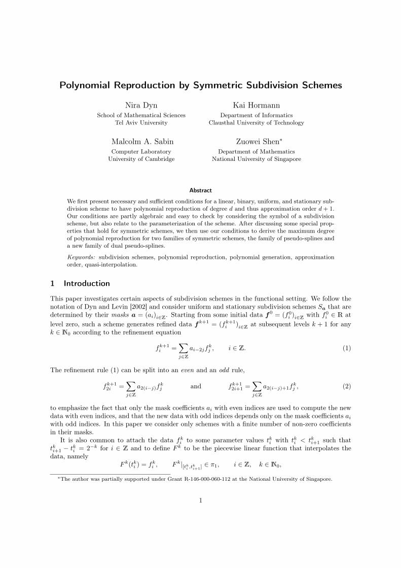
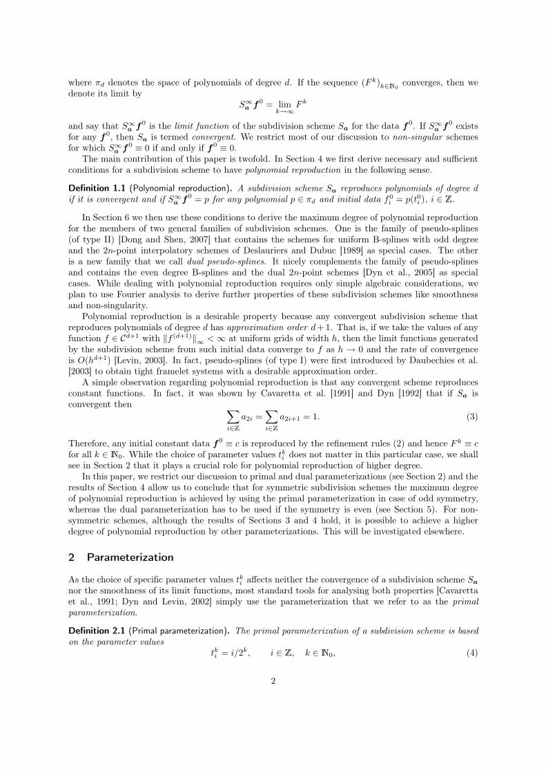
Figure 1: Primal parameterization.

i i+1i¡1

if0

i+1f0

i+2f0

i¡1f0

2i¡1f1 2if1

2i+1f1 2i+2f1

2i+3f1 2i¡2f1

F 0

F 1

Figure 2: Dual parameterization.

so that tk+12i = tki and tk+1

2i+1 = (tki + tki+1)/2. Accordingly, we can say that each subdivision step replacesthe old data fk

i by the new data fk+12i with even indices and the new data fk+1

2i+1 with odd indices is addedhalfway between the old data fk

i and fki+1 (see Figure 1).

But in so far as the polynomial reproduction property of Sa is concerned, this parameterization doesnot always yield the highest degree possible. Motivated by the following example, we also consider thedual parameterization in this paper.

Definition 2.2 (Dual parameterization). The dual parameterization of a subdivision scheme attaches thedata fk

i to the parameter values

tki = (i− 12 )/2k, i ∈ Z, k ∈ N0, (5)

with tk+12i−1 = (tki−1 + 3tki )/4 and tk+1

2i = (3tki + tki+1)/4. In this setting, each subdivision step replacesthe old data fk

i by the new data fk+12i−1 and fk+1

2i , one to the left, the other to the right, and both at onequarter the distance to the neighbours fk

i−1 and fki+1 (see Figure 2).

Note that the parameter values in (4) and (5) differ only by a shift of 1/2k+1 that vanishes as k →∞,so that the limit function S∞a f0 for any fixed initial data f0 is the same, no matter which of the twoparameterizations is used. However, in the context of polynomial reproduction there still remains animportant difference, because the initial data with respect to the primal parameterization is f0

i = p(i),whereas f0

i = p(i− 1/2) is used in the case of the dual parameterization.

3

For example, let us consider the uniform linear B-spline scheme with mask [a−1, a0, a1] = [ 12 , 1, 12 ]

and assume the initial data to be sampled from the linear polynomial p(x) = x, that is, f0i = t0i . If the

primal parameter values in (4) are used, then it is easy to see that (S∞a f0)(x) = x, whereas the dualparameter values in (5) give the limit function x − 1/2. On the other hand, the limit function of theuniform quadratic B-spline scheme with mask [a−2, a−1, a0, a1] = [14 , 3

4 , 34 , 1

4 ] is x + 1/2 for the primaland x for the dual parameterization. Both examples are special cases of schemes with a symmetricmask, and we shall come back to such schemes in Section 5.

3 Polynomial Generation

An obvious necessary condition for a subdivision scheme Sa to reproduce polynomials of degree d isthat it must be able to generate polynomials of the same degree as limit functions for some initial data.For the kind of subdivision schemes that we consider, this property is equivalent to a simple conditionon the mask a that can best be stated by using the algebraic formalism of z-transforms.

Definition 3.1 (z-transform). For any sequence c = (ci)i∈Z we denote by

c(z) =∑i∈Z

cizi

its z-transform and the even and odd components of the z-transform by

ce(z) =∑i∈Z

c2iz2i and co(z) =

∑i∈Z

c2i+1z2i+1.

Obviously,c(z) = ce(z) + co(z), ce(z) =

(c(z) + c(−z)

)/2,

c(−z) = ce(z)− co(z), co(z) =(c(z)− c(−z)

)/2.

(6)

Moreover, we can now write the refinement rule (1) as

fk+1(z) = a(z)fk(z2) (7)

and the even and odd rules (2) as

fk+1e (z) = ae(z)fk(z2) and fk+1

o (z) = ao(z)fk(z2).

Note that the z-transform a(z) of the mask a is usually called the symbol of the scheme Sa and thata(z) is a Laurent polynomial, as we consider only schemes with masks consisting of a finite number ofnon-zero coefficients.

Theorem 3.2 (Polynomial generation). For a non-singular subdivision scheme Sa the condition

(PG) a(z) is divisible by (1 + z)dG+1

is equivalent to the property that there exists for any polynomial p of degree d ≤ dG some initial dataf0 such that S∞a f0 = p. Moreover, f0 is sampled from a polynomial of the same degree and with thesame leading coefficient. In other words, there exists some q ∈ πd such that f0

i = q(t0i ) for i ∈ Z andp− q ∈ πd−1.

This theorem is proved in a more general setting by Cavaretta et al. [1991, Chapter 6]

Remark 3.3. The non-singularity of the scheme Sa is actually not required for the sufficiency of con-dition (PG) for polynomial generation, but only needed to show its necessity (see also Dyn and Levin[2002] and [Warren and Weimer, 2001, Theorem 3.7]).

Levin [2003] showed that any subdivision scheme Sa that generates polynomials of degree d canalso reproduce polynomials of the same degree if the initial data is pre-processed by a suitable linearoperator Q, so that the combination of S∞a and Q gives a quasi-interpolation operator with optimalapproximation order d + 1. In the next section, however, we derive conditions on the symbol a(z) thatguarantee Sa to reproduce polynomials up to degree d without the need for any pre-processing.

4

4 Polynomial Reproduction

Let us start by introducing the following definition of data that is generated by uniformly sampling apolynomial.

Definition 4.1 (Polynomial data). A sequence g = (gi)i∈Z is called polynomial data of degree d if thereexists a polynomial p ∈ πd such that gi = p(i) for all i ∈ Z.

If we denote by ∆` the `-th order finite difference operator on sequences,

∆`g = (∆`gi)i∈Z with ∆`gi =∑j=0

(−1)j

(`

j

)gi−j ,

then such polynomial data is characterized by having vanishing finite differences of order d + 1, namely

∆d+1g ≡ 0,

which in terms of z-transforms translates to the condition

(1− z)d+1g(z) = 0. (8)

Interestingly, (1− z)d+1 is essentially the only Laurent polynomial that annihilates the z-transforms ofall polynomial data of degree d.

Lemma 4.2. The Laurent polynomial b(z) is divisible by (1− z)d+1 if and only if

b(z)g(z) = 0 (9)

for any polynomial data g of degree d.

Proof. The necessity of condition (9) follows immediately from (8). In order to show the sufficiency wewill prove by induction that there exist Laurent polynomials r0, . . . , rd such that

b(z) = (1− z)k+1rk(z) (10)

for k = 0, . . . , d. We start with k = 0 and let g be any polynomial data of degree 0 so that its z-transformis

g(z) = c∑i∈Z

zi

for some c ∈ R. Then

b(z)g(z) =( ∑

i∈Zbiz

i)(

c∑j∈Z

zj)

= c∑j∈Z

zj( ∑

i∈Zbi

)= 0

for any c ∈ R and therefore ∑i∈Z

bi = b(1) = 0.

In other words, b(z) has a root at z = 1 and there exists some r0(z) with b(z) = (1− z)r0(z).Now assume that (10) holds for some k < d and let g be any polynomial data of degree k + 1.

By taking the finite differences of degree k + 1 of g we get the constant sequence f = ∆k+1g withz-transform

f(z) = (1− z)k+1g(z).

From (9) and (10) we then have

b(z)g(z) = rk(z)(1− z)k+1g(z) = rk(z)f(z) = 0,

and with the same arguments as in the case k = 0 we conclude that there exists some rk+1(z) withrk(z) = (1− z)rk+1(z). Therefore,

b(z) = (1− z)k+1rk(z) = (1− z)k+2

rk+1(z),

which completes the induction step.

5

The following equivalence then is an immediate consequence of Theorem 3.2 and Lemma 4.2.

Corollary 4.3. A subdivision scheme Sa generates polynomials of degree d if and only if

a(z)g(−z) = 0 (11)

for any polynomial data g of degree d.

Proof. Theorem 3.2 states that the symbol a(z) of a subdivision scheme that generates polynomials ofdegree d is divisible by (1 + z)d+1 so that the Laurent polynomial b(z) = a(−z) is divisible by (1− z)d+1.By Lemma 4.2 this is equivalent to the property that b(z)g(z) = a(−z)g(z) = 0 for any polynomialdata g of degree d, hence the statement follows by replacing z with −z in (11).

We further need the notion of stepwise polynomial reproduction, which is in fact equivalent topolynomial reproduction in the limit for non-singular subdivision schemes.

Definition 4.4 (Stepwise polynomial reproduction). We say that Sa reproduces polynomial data of degreed in each subdivision step if the data fk with fk

i = p(tki ) is refined to fk+1 with fk+1i = p(tk+1

i ), i ∈ Zfor any p ∈ πd and k ∈ N0.

Corollary 4.5. A subdivision scheme Sa that reproduces polynomial data of degree d in each subdivisionstep also reproduces polynomials of degree d and vice versa.

Proof. For any p ∈ πd let f0 be the initial data with f0i = p(t0i ), i ∈ Z. If Sa reproduces this data in

each subdivision step, then

F k(tki ) = fki = p(tki ), i ∈ Z, k ∈ N0,

so that (F k)k∈N0is a sequence of piecewise linear approximations to p over uniform grids of width

h(k) = 1/2k and thus clearly converges to p as k →∞.We now assume that Sa reproduces polynomials of degree d and let k ∈ N0. On the one hand,

applying the subdivision scheme to the data fk with fki = p(tki ) gives p = S∞a fk = S∞a fk+1, but on

the other we also get p = S∞a gk+1 as the limit function for the data gk+1 with gk+1i = p(tk+1

i ). By thelinearity of the operator S∞a we then have S∞a (fk+1 − gk+1) ≡ 0 and as we consider only non-singularschemes, this implies fk+1 = gk+1.

Note that a similar equivalence holds between stepwise polynomial generation and the generationof polynomials in the limit. We can now establish our conditions for the reproduction of polynomialsthat are similar to the one for polynomial generation in Theorem 3.2.

Theorem 4.6 (Primal polynomial reproduction). If Sa is a subdivision scheme that generates polynomialsof degree dG, then it reproduces polynomials of degree dR ≤ dG with respect to the primal parameteriza-tion if and only if

(PR1) a(z)− 2 is divisible by (1− z)dR+1.

Proof. Because of Corollary 4.5, it suffices to show that condition (PR1) is equivalent to the propertythat Sa reproduces polynomial data of degree dR in each subdivision step. To this end, let tki be theparameter values from (4) and p ∈ πdR , so that the sequences fk and g with fk

i = p(tki ) and gi = p(tk+1i ),

i ∈ Z are both polynomial data of degree dR. Since fki = g2i, we have

fk(z2) =∑i∈Z

fki z2i =

∑i∈Z

g2iz2i = ge(z) =

(g(z) + g(−z)

)/2

and refining the data fk with the subdivision scheme gives, in view of (7),

fk+1(z) = a(z)fk(z2) = a(z)g(z)/2 + a(z)g(−z)/2 = a(z)g(z)/2,

6

where the last identity follows from (11). On the other hand, g(z) = fk+1(z), and hence the data fk isreproduced by subdivision with Sa if and only if

a(z)g(z) = 2g(z),

which, according to Lemma 4.2, is equivalent to (PR1).

Theorem 4.7 (Dual polynomial reproduction). If Sa is a subdivision scheme that generates polynomialsof degree dG, then it reproduces polynomials of degree dR ≤ dG with respect to the dual parameterizationif and only if

(PR2) a(z2)z − 2 is divisible by (1− z)dR+1

Proof. Due to Corollary 4.5, it is again sufficient to show that condition (PR2) is equivalent to theproperty of stepwise polynomial reproduction. Let tki be the parameter values from (5) and p ∈ πdR ,so that the sequences fk, g, and h with fk

i = p(tki ), gi = p((i− 1)/2k+1), and hi = p((i− 1)/2k+2) fori ∈ Z are all polynomial data of degree dR. Since fk

i = g2i, we conclude as in the proof of Theorem 4.6that

fk+1(z) = a(z)g(z)/2. (12)

Noting that gi = h2i−1, we further have

g(z2) =∑i∈Z

giz2i =

∑i∈Z

h2i−1z2i−1z = ho(z)z (13)

and thereforefk+1(z2) = a(z2)ho(z)z/2.

If (PR2) holds, then we know from Lemma 4.2 that

a(z2)h(z)z = 2h(z)

and thereforea(z2)h(−z)z = −2h(−z)

for any polynomial data h of degree dR. Thus

fk+1(z2) = a(z2)ho(z)z/2 =(a(z2)h(z)z − a(z2)h(−z)z

)/4 =

(h(z) + h(−z)

)/2 = he(z).

Comparing the coefficients of fk+1(z2) and he(z), we see that fk+1i = h2i = p(tk+1

i ) for all i ∈ Z,hence Sa reproduces polynomials of degree dR. On the other hand, if the scheme has the property thatfk+1

i = h2i, then by (12) and (13) we have

a(z2)ho(z)z/2 = he(z)

for any polynomial data h of degree dR and in particular for the data h with hi = hi+1, so that

a(z2)he(z)z/2 = a(z2)ho(z)z2/2 = he(z)z = ho(z).

Combining both identities then gives

a(z2)h(z)z =(a(z2)he(z)z + a(z2)ho(z)z

)= 2

(ho(z) + he(z)

)= 2h(z)

and condition (PR2) follows from Lemma 4.2.

Remark 4.8. Note that the non-singularity of the scheme Sa is only needed in the second half of theproof of Corollary 4.5 and is thus not required for the sufficiency of the conditions (PR1) and (PR2) forpolynomial reproduction.

7

As mentioned above, the degree dR of polynomial reproduction can never exceed the degree dG ofpolynomial generation. We shall now derive an interesting observation in the case that dG > dR. FromTheorem 3.2 we know that for any polynomial p of degree d with dG ≥ d > dR there exists somepolynomial q ∈ πd such that p is the limit function for the initial data f0 sampled from q, and thatp− q ∈ πd−1. The examples from Levin [2003] further suggest that even the two leading coefficients ofp and q agree, that is, p− q ∈ πd−2. This is in fact confirmed by the following more general statement.

Corollary 4.9. Let Sa be a convergent subdivision scheme with generation degree dG and reproductiondegree dR. If p and q are polynomials of degree d ≤ dG such that p = S∞a f0 for f0

i = q(t0i ), i ∈ Z, thenp and q have the same dR + 1 leading coefficients.

Proof. We start by extending the definition of the finite difference operator ∆` to functions, that is,

(∆`f)(x) =∑j=0

(−1)j

(`

j

)f(x− j).

A useful identity that follows immediately from the linearity of the operator S∞a and the relation

(S∞a f0·+i)(x) = (S∞a f0)(x + i)

is that the operators S∞a and ∆` commute [Dyn and Levin, 2002],

∆`(S∞a f0) = S∞a (∆`f0). (14)

Now let g0 = ∆d−dRf0 be the polynomial data of degree dR that is sampled from the polynomial∆d−dRq. It then follows from the reproduction property of Sa that the corresponding limit function is

S∞a g0 = ∆d−dRq.

Due to (14) we also have

∆d−dRp = ∆d−dR(S∞a f0) = S∞a (∆d−dRf0) = S∞a g0,

and conclude that ∆d−dR(p − q) ≡ 0. This implies that the degree of the polynomial p − q is at mostd− dR − 1 and so the first dR + 1 leading coefficients of p and q must be identical.

5 Symmetric Schemes

Let us now investigate the conditions for reproduction of polynomials of low degree in more detail.According to condition (PG), the generation of constant functions requires the symbol a(z) to have azero at z = −1, and it follows from conditions (PR1) and (PR2) that the scheme further reproducesthese functions with respect to the primal as well as the dual parameterization if and only if a(1) = 2.Combining both conditions, a subdivision scheme Sa reproduces constant polynomials if and only if

a(−1) = 0 and a(1) = 2 ⇐⇒ ae(1) = ao(1) = 1,

where the equivalence to the conditions on the right follows from (6). Note that these latter conditionsare further equivalent to the ones in Equation (3) and thus confirm our previous observation that anyconvergent subdivision scheme reproduces constant functions, regardless of the chosen parameterization.

To check reproduction of linear polynomials we have to find out if the roots z = 1 and z = −1 aredouble roots of a(z) and a(z) − 2 (or a(z2)z − 2), respectively. It then follows that any scheme withconstant reproduction also reproduces linear functions if and only if

a′(−1) = 0 and a′(1) = 0 (or a′(1) = −1), (15)

8

where the two options in the second condition refer to the primal and the dual parameterization, respec-tively. Obviously, a scheme cannot reproduce linear functions with respect to both parameterizations,and the value a′(1) actually tells which of the two should be chosen.

For example, the uniform degree m B-spline schemes all reproduce constant functions, because theirgeneral symbol

bm(z) = 2−m(1 + z)m+1zn, n ∈ Z,

clearly fulfills the conditions bm(−1) = 0 and bm(1) = 2. For m > 0 we further have b′m(−1) = 0 andb′m(1) = m + 1 + 2n. Now, by appropriately shifting the symbol with the choice n = −dm+1

2 e, b′m(1)evaluates to 0 for odd m and to −1 for even m, thus confirming the known fact that all but the piecewiseconstant B-splines reproduce linear functions with respect to the appropriate parameterization.

The B-spline schemes are particular examples of odd and even symmetric subdivision schemes,and we can show more generally which parameterization to choose in order to have at least linearreproduction.

Definition 5.1 (Symmetric schemes). A subdivision scheme Sa is called odd symmetric if

a−i = ai, i ∈ Z,

and even symmetric ifa−i = ai−1, i ∈ Z.

In terms of Laurent polynomials, these conditions translate to a(z) = a(1/z) and a(z)z = a(1/z),respectively.

Corollary 5.2. In order to achieve as high degrees of polynomial reproduction as possible, the primalparameterization should be used for odd symmetric schemes and the dual parameterization for schemeswith even symmetry.

Proof. If Sa is odd symmetric, then by taking the derivative on both sides of the condition a(z) = a(1/z)we get

a′(z) = −a′(1/z)/z2,

which implies a′(−1) = a′(1) = 0. Thus, according to (15), it is impossible for an odd symmetricscheme to reproduce linear functions with respect to the dual parameterization. However, linear repro-duction with respect to the primal parameterization comes for free for any such scheme that reproducesconstants.

If Sa is even symmetric, then the condition a(z)z = a(1/z) gives

a′(z)z + a(z) = −a′(1/z)/z2.

In particular a(−1) = 0 and a′(1) = −a(1)/2. Hence, if the scheme reproduces constants then a′(1) =−1, so that linear functions with respect to the primal parameterization cannot be reproduced. On theother hand, linear reproduction with respect to the dual parameterization is guaranteed for all evensymmetric schemes that reproduce constants and generate linear polynomials.

These observations encourage us to always use the appropriate parameterization for odd and evensymmetric schemes by default and call them primal and dual schemes, respectively.

In the proof of the previous corollary some of the conditions for the generation and reproductionof linear functions follow directly from the symmetry of the schemes. These are in fact special casesof two more general propositions regarding the degrees of polynomial generation and reproduction ofsymmetric schemes.

Corollary 5.3. A symmetric subdivision scheme Sa generates polynomials up to a degree of the sameparity as the parity of its symmetry.

9

Proof. Let dG be the maximal degree of polynomial generation of the scheme Sa. Then, according tocondition (PG), there exists a Laurent polynomial r(z) such that

a(z) = (1 + z)dG+1r(z).

For a scheme with odd symmetry we have

a(z) = a(1/z) = (1 + 1/z)dG+1r(1/z) = (1 + z)dG+1

z−dG−1r(1/z),

so thatzdG+1r(z) = r(1/z).

If we assume dG to be even, then substituting z = −1 gives

−r(−1) = r(−1),

showing that r(z) contains 1 + z as a factor, which in turn contradicts the assumption that dG ismaximal. Therefore, dG is always odd for schemes with odd symmetry and a similar argument showsthat dG is always even for schemes with even symmetry.

Corollary 5.4. Let Sa be a symmetric subdivision scheme with the appropriate parameterization. ThenSa reproduces polynomials up to an odd degree, provided that it generates polynomials up to that degree.

Proof. Let dR be the maximal degree of polynomial reproduction of Sa. Conditions (PR1) and (PR2)then imply the existence of a Laurent polynomial r(z) with

a(z)− 2 = (1− z)dR+1r(z)

if Sa is odd symmetric and with

a(z2)z − 2 = (1− z)dR+1r(z)

in case of even symmetry. Using the properties that a(z) = a(1/z) for odd and a(z2)z = a(1/z2)/z foreven symmetric schemes, we conclude in both cases that

(1− z)dR+1r(z) = (1− 1/z)dR+1

r(1/z),

leading to(−z)dR+1

r(z) = r(1/z).

Assuming dR to be even and substituting z = 1 then yields

−r(1) = r(1),

so that r(z) is divisible by 1− z, contradicting the assumption that dR is maximal.

6 Two Families of Symmetric Subdivision Schemes

As an application of our results, we shall now derive the degree of polynomial reproduction for themembers of a known family of primal subdivision schemes Sal

mand a new family of dual subdivision

schemes Salm

. We define the Laurent polynomials

σ(z) =(1 + z)2

4z, δ(z) = − (1− z)2

4z, (16)

and note that σ(z) and δ(z) fulfill the two identities

σ(z) + δ(z) = 1 and δ(z2) = 4σ(z)δ(z). (17)

10

Then the symbols of the primal schemes are

alm(z) = 2 σ(z)m

l∑i=0

(m + l

i

)δ(z)i

σ(z)l−i, (18)

whereas those of the dual schemes are

alm(z) =

1 + z

zσ(z)m

l∑i=0

(m + 1/2 + l

i

)δ(z)i

σ(z)l−i, (19)

with m, l ≥ 0. It follows directly from σ(1/z) = σ(z) and δ(1/z) = δ(z) that the schemes Salm(z) and

Salm(z) are odd and even symmetric, respectively.We note that as shown in Dong and Shen [2006b, Equation (2.5)], the primal schemes are equivalent

to the pseudo-splines of type II that were introduced by Dong and Shen [2007] for the construction ofsymmetric framelets whose truncated framelet series has a desirable approximation order.

Theorem 6.1. The primal subdivision schemes with symbols alm(z) reproduce polynomials up to degree

min(2m− 1, 2l + 1).

Proof. It follows directly from (18) that alm(z) is divisible by (1 + z)2m, hence the scheme generates

polynomials of degree 2m−1. It is further clear that this is the maximal degree of polynomial generationbecause the remainder r(z) = al

m(z)/(1 + z)2m evaluates to r(−1) = 2(−1/4)m(m+l

l

)6= 0 at z = −1.

According to (17) we have (σ + δ)m+l = 1 and by applying the binomial theorem to the left hand side,we can write al

m(z) as

alm(z) = 2− 2

m+l∑i=l+1

(m + l

i

)δ(z)i

σ(z)m+l−i = 2− 2 δ(z)l+1m∑

i=1

(m + l

i + l

)δ(z)i−1

σ(z)m−i,

showing that alm(z)−2 is clearly divisible by (1− z)2l+2. This is again maximal, because the remainder

r(z) = (alm(z)− 2)/(1− z)2l+2 evaluates to r(1) = −2(−1/4)l+1(m+l

1+l

)6= 0. The statement then follows

from Theorems 3.2 and 4.6.

This result was first shown by Dong and Shen [2007, Theorem 3.10] using a Fourier analysis approach.Dong and Shen also noted that a0

m(z) = b2m−1(z), m ≥ 1 are the symbols of the odd degree B-splinesand that an−1

n (z), n ≥ 1 are those of the 2n-point interpolatory schemes of Deslauriers and Dubuc[1989]. Moreover, it is straightforward to verify that the symbols of the schemes S2L(ω), L ≥ 1 in[Choi et al., 2006] are affine combinations of aL−1

L+1(z) and aL−1L (z) with weights αL(ω) = ω16L/

(2LL

)and 1−αL(ω) and that a1

k(z) are the symbols of the schemes S2k, k ≥ 2 in [Hormann and Sabin, 2007].

Theorem 6.2. The dual subdivision schemes with symbols alm(z) reproduce polynomials up to degree

min(2m, 2l + 1).

Proof. For any real α > 0 and |x| ≤ 1,

(1 + x)α =∞∑

i=0

(α

i

)xi.

Now by (17),

1 =(σ(z2) + δ(z2)

)m+1/2+l= σ(z2)

m+1/2+l(

1 +δ(z2)σ(z2)

)m+1/2+l

,

and since δ(z2)σ(z2) ∈ [−1, 0] for real z, we have

1 =1 + z2

2zσ(z2)

m∞∑

i=0

(m + 1/2 + l

i

)δ(z2)

iσ(z2)

l−i.

11

Using (19) we can rewrite the above equality as

2− alm(z2)z =

1 + z2

zδ(z2)

l+1∞∑

i=l+1

(m + 1/2 + l

i

)δ(z2)

i−l−1σ(z2)

m+l−i.

According to (17), δ(z2)l+1 = 4l+1δ(z)l+1σ(z)l+1, and we get

2− alm(z2)z = δ(z)l+1

R(z),

with

R(z) =1 + z2

z4l+1σ(z)l+1

∞∑i=l+1

(m + 1/2 + l

i

)δ(z2)

i−l−1σ(z2)

m+l−i.

By (16), σ(1) = 1 and δ(1) = 0, and thus

R(1) = 22l+3

(m + 1/2 + l

l + 1

)6= 0.

On the other hand, R(z) is the rational function

R(z) =2− al

m(z2)z

δ(z)l+1.

These two properties of R imply that the numerator of R is divisible by exactly 2l + 2 factors 1 − z.The claim of the theorem now follows from Theorems 3.2 and 4.7.

Like the family of primal schemes, this new family of dual schemes also has some well-known specialcases. The symbols of the even degree B-splines are a0

m(z) = b2m(z), m ≥ 0, those of the schemesS2L−1(ω), L ≥ 1 in [Choi et al., 2006] are affine combinations of aL−1

L (z) and aL−1L−1(z) with weights

αL(ω) = ω42L−1/(2L−3/2

L−1

)and 1 − αL(ω), and a1

k(z) are the symbols of the schemes S2k+1, k ≥ 1 in[Hormann and Sabin, 2007]. Moreover, an−1

n , n ≥ 1 are the symbols of the dual 2n-point schemes ofDyn et al. [2005], which are based on interpolating 2n successive data points fk

i−n+1, . . . , fki+n at the

dual parameter values tki−n+1, . . . , tki+n from (5) by a polynomial of degree 2n− 1 and then evaluating

this polynomial at tk+12i and tk+1

2i+1 to determine the new data fk+12i and fk+1

2i+1. We found that a similarconstruction yields the symbols an−1

n−1 of the dual (2n− 1)-point schemes for n ≥ 1. Here a polynomialof degree 2n− 2, interpolating the 2n− 1 points (tkj , fk

j ), |j − i| ≤ n− 1 is constructed, and fk+12i−1, fk+1

2i

are the values of this polynomial at tk+12i−1, tk+1

2i , respectively. In this construction the parameterizationis again the dual one.

Finally, we would like to note that by using the identity

l∑i=0

(r + i

i

)xi =

l∑i=0

(r + 1 + l

i

)xi(1− x)l−i

,

which can be proved straightforwardly by induction over l for any r, x ∈ R, the symbols from bothfamilies can be expressed in a slightly more compact form, namely

alm(z) = 2 σ(z)m

l∑i=0

(m− 1 + i

i

)δ(z)i

and

alm(z) =

1 + z

zσ(z)m

l∑i=0

(m− 1/2 + i

i

)δ(z)i

.

This form of alm(z) also appears in the papers by Dong and Shen [2006a, 2007].

12

References

A. S. Cavaretta, W. Dahmen, and C. A. Micchelli. Stationary subdivision. Memoirs of the AmericanMathematical Society, 93(453):vi+186, 1991.

S. W. Choi, B.-G. Lee, Y. J. Lee, and J. Yoon. Stationary subdivision schemes reproducing polynomials.Computer Aided Geometric Design, 23(4):351–360, May 2006.

I. Daubechies, B. Han, A. Ron, and Z. Shen. Framelets: MRA-based constructions of wavelet frames.Applied and Computational Harmonic Analysis, 14(1):1–46, Jan. 2003.

G. Deslauriers and S. Dubuc. Symmetric iterative interpolation processes. Constructive Approximation,5(1):49–68, Dec. 1989.

B. Dong and Z. Shen. Construction of biorthogonal wavelets froms pseudo-splines. Journal of Approx-imation Theory, 138(2):211–231, Feb. 2006a.

B. Dong and Z. Shen. Linear independence of pseudo-splines. Proceedings of the American MathematicalSociety, 134(9):2685–2694, Sept. 2006b.

B. Dong and Z. Shen. Pseudo-splines, wavelets and framelets. Applied and Computational HarmonicAnalysis, 22(1):78–104, Jan. 2007.

N. Dyn. Subdivision schemes in computer-aided geometric design. In W. Light, editor, Advances innumerical analysis, volume II, pages 36–104. Oxford University Press, New York, 1992.

N. Dyn, M. S. Floater, and K. Hormann. A C2 four-point subdivision scheme with fourth order accuracyand its extensions. In M. Dæhlen, K. Mørken, and L. L. Schumaker, editors, Mathematical Methodsfor Curves and Surfaces: Tromsø 2004, Modern Methods in Mathematics, pages 145–156. NashboroPress, Brentwood, TN, 2005.

N. Dyn and D. Levin. Subdivision schemes in geometric modelling. Acta Numerica, 11:73–144, Jan.2002.

K. Hormann and M. A. Sabin. A family of subdivision schemes with cubic precision. Computer AidedGeometric Design, 2007. To appear.

A. Levin. Polynomial generation and quasi-interpolation in stationary non-uniform subdivision. Com-puter Aided Geometric Design, 20(1):41–60, Mar. 2003.

J. Warren and H. Weimer. Subdivision Methods for Geometric Design: A Constructive Approach.The Morgan Kaufmann Series in Computer Graphics and Geometric Modeling. Morgan KaufmannPublishers, San Francisco, 2001.

13