Embed Size (px)
Citation preview
1
Polymerase Chain Reaction Endpoint and Quantitative Real Time RT-PCR
by Justin M. Fear, Aline Bonilla and Peter J. Hansen
Table of Contents What is PCR? ............................................................................................................................................ 2 Choice of Analytical Approach .................................................................................................................. 3 Sample Collection ...................................................................................................................................... 4
Embryo Collection ................................................................................................................................ 4 Cell Collection ....................................................................................................................................... 5
RNA Extraction .......................................................................................................................................... 7 Embryos ................................................................................................................................................ 7 Cells ....................................................................................................................................................... 8
Determination of RNA Concentration and Quality.................................................................................. 11 RNA Concentration Using NanoDrop ................................................................................................. 11 RNA Concentration and Quality using the Bioanalyzer ..................................................................... 12
DNase Treatment...................................................................................................................................... 13 Reverse Transcription (RT) For Real-Time PCR ..................................................................................... 15 Quantitative Real-Time PCR using Sybr Green ...................................................................................... 17
Running a Standard Curve .................................................................................................................. 17 Running Samples ................................................................................................................................. 20 Using Applied Biosystems Real-Time PCR ........................................................................................ 22
End Point PCR ......................................................................................................................................... 23 Using One-Step Reverse Transcription ............................................................................................... 23 Agarose Gel Electrophoresis ............................................................................................................... 24
Acknowledgments .................................................................................................................................... 28 References ................................................................................................................................................ 28 Appendix .................................................................................................................................................. 29
Other Reagents .................................................................................................................................... 29 Alternative RNA Extraction ................................................................................................................ 30 Using a Hemocytometer ...................................................................................................................... 32 Primers ................................................................................................................................................ 34 Real-Time PCR Analysis ..................................................................................................................... 39
2
Choice of Analytical Approach The first step before starting a reverse transcriptase PCR (RT-PCR) experiment is to determine the appropriate endpoint. There are two major forms of RT-PCR. One involves running the PCR product out on a gel and visualizing the product (called endpoint RT-PCR). The other involves the use of a fluorescent dye and a Real-time PCR machine to measure dye incorporation that, in turn, is proportional to amount of template cDNA (called Real-Time RT-PCR). Both methodologies allow for either relative or quantitative measurements depending on how the experiment is designed. Our laboratory typically uses endpoint RT-PCR for a few specific assays (i.e. sexing embryos) and to test primers before use (i.e. visualize product either from an endpoint reaction or real-time reaction to very the production of only one product). For most of our RT-PCR needs it is preferred to use the real-time RT-PCR method. Quantification is more accurate with real-time RT-PCR and data are more easily publishable when amounts of mRNA have been quantified with this method than with endpoint RT-PCR. Many of the steps for RT-PCR are similar for both methods. The first decision is the choice of genes to measure. Besides genes of interest, 1-4 genes should be measured as internal controls to control for RNA recovery. These housekeeping genes are typically genes that are constitutively expressed in a manner where treatment is unlikely to cause a change in expression. The housekeeping gene is very important and its appropriateness can determine the accuracy of data analysis. Some typical housekeeping genes include GAPDH, β-actin, tubulin, 18s, and Histone H2A.1. The advantage of analyzing more than one housekeeping gene is that problems arising from treatment effects on the housekeeping gene are avoided. If occurring, other housekeeping genes are available for analysis. Some other labs also incorporate exognenous genes to act as standards (i.e. GFP) but that is beyond the scope of this manual. Once genes of interest and appropriate housekeeping genes have been selected, proper primer design is essential. Typically it is easiest to find primers published in the literature using similar experimental conditions. However many times, it is necessary to design sets of primers. Refer to the Primer Design section in the Appendix for some basic instructions on how to design and order primers, the Primer Dilution section for instructions on diluting primers, and the Primer Validation section for an overview on how to validate a new primer. While designing and testing primers, the basic work flow for a RT-PCR experiment is as follow:
I. Begin experiment and proceed to Sample Collection II. Once samples are collected proceed to RNA Extraction.
III. After RNA Extraction, measure the amount of RNA (see Determination of RNA Concentration and Quality)
IV. Remove any DNA contaminants from the RNA samples by DNase Treatment. V. Perform Endpoint RT-PCR or Quantitative Real-Time PCR using Sybr Green.
VI. For endpoint RT-PCR, perform Agarose Gel Electrophoresis. For real-time RT-PCR, perform Real-Time PCR Analysis.
3
Sample Collection Note: Sample collection varies depending on which model you are using (i.e. embryos, cells, or tissue). This section will cover various methods of sample collection. You should work as clean as possible (i.e. wear gloves and bleach work area).
Embryo Collection
Materials • 1.5 mL centrifuge tube (RNase Free)
o Autoclaved and cross-linked with UV light (120 sec) • Grid Plate (BD Falcon 351112) • Liquid Nitrogen • Latex gloves • PBS-PVP (1 mg/mL)
o 13 mL PBS + NaCl (See Other Reagents) o 13 mg polyvinylpyrrolidone (Kodak 15420)
• 0.1% DEPC H2O o 1 mL Diethyl Pyrocarbonate (DEPC) (Sigma D5758) o 1000 mL H2O o Mix overnight at 37ºC o Autoclave 30 min 15 psi
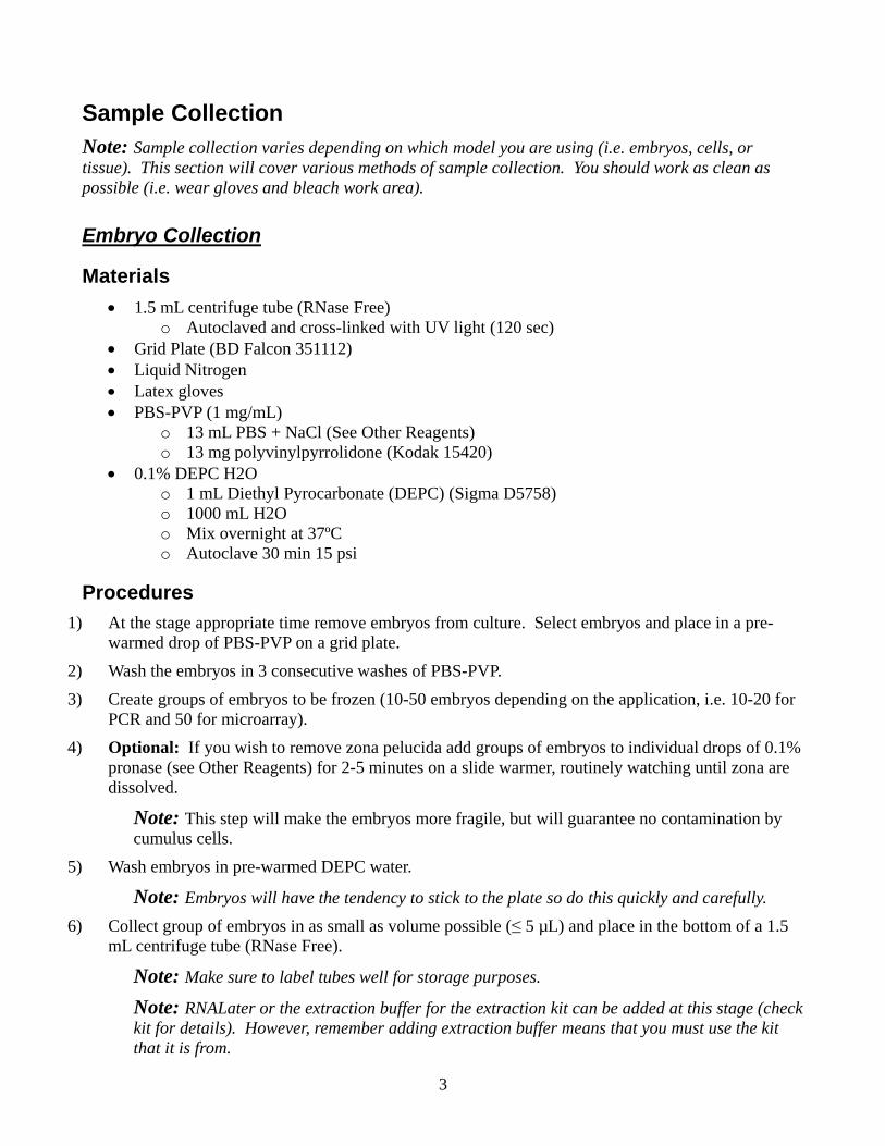
Procedures 1) At the stage appropriate time remove embryos from culture. Select embryos and place in a pre-
warmed drop of PBS-PVP on a grid plate. 2) Wash the embryos in 3 consecutive washes of PBS-PVP. 3) Create groups of embryos to be frozen (10-50 embryos depending on the application, i.e. 10-20 for
PCR and 50 for microarray). 4) Optional: If you wish to remove zona pelucida add groups of embryos to individual drops of 0.1%
pronase (see Other Reagents) for 2-5 minutes on a slide warmer, routinely watching until zona are dissolved.
Note: This step will make the embryos more fragile, but will guarantee no contamination by cumulus cells.
5) Wash embryos in pre-warmed DEPC water.
Note: Embryos will have the tendency to stick to the plate so do this quickly and carefully. 6) Collect group of embryos in as small as volume possible (≤ 5 µL) and place in the bottom of a 1.5
mL centrifuge tube (RNase Free).
Note: Make sure to label tubes well for storage purposes.
Note: RNALater or the extraction buffer for the extraction kit can be added at this stage (check kit for details). However, remember adding extraction buffer means that you must use the kit that it is from.
4
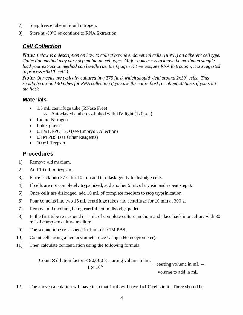
7) Snap freeze tube in liquid nitrogen. 8) Store at -80ºC or continue to RNA Extraction.
Cell Collection Note: Below is a description on how to collect bovine endometrial cells (BEND) an adherent cell type. Collection method may vary depending on cell type. Major concern is to know the maximum sample load your extraction method can handle (i.e. the Qiagen Kit we use, see RNA Extraction, it is suggested to process ~5x10⁵ cells). Note: Our cells are typically cultured in a T75 flask which should yield around 2x10⁷ cells. This should be around 40 tubes for RNA collection if you use the entire flask, or about 20 tubes if you split the flask.
Materials • 1.5 mL centrifuge tube (RNase Free)
o Autoclaved and cross-linked with UV light (120 sec) • Liquid Nitrogen • Latex gloves • 0.1% DEPC H2O (see Embryo Collection) • 0.1M PBS (see Other Reagents) • 10 mL Trypsin
Procedures 1) Remove old medium. 2) Add 10 mL of trypsin. 3) Place back into 37ºC for 10 min and tap flask gently to dislodge cells. 4) If cells are not completely trypsinized, add another 5 mL of trypsin and repeat step 3. 5) Once cells are dislodged, add 10 mL of complete medium to stop trypsinization. 6) Pour contents into two 15 mL centrifuge tubes and centrifuge for 10 min at 300 g. 7) Remove old medium, being careful not to dislodge pellet. 8) In the first tube re-suspend in 1 mL of complete culture medium and place back into culture with 30
mL of complete culture medium. 9) The second tube re-suspend in 1 mL of 0.1M PBS.
10) Count cells using a hemocytometer (see Using a Hemocytometer). 11) Then calculate concentration using the following formula:
Count dilution factor 50,000 starting volume in mL
1 10 starting volume in mL
volume to add in mL
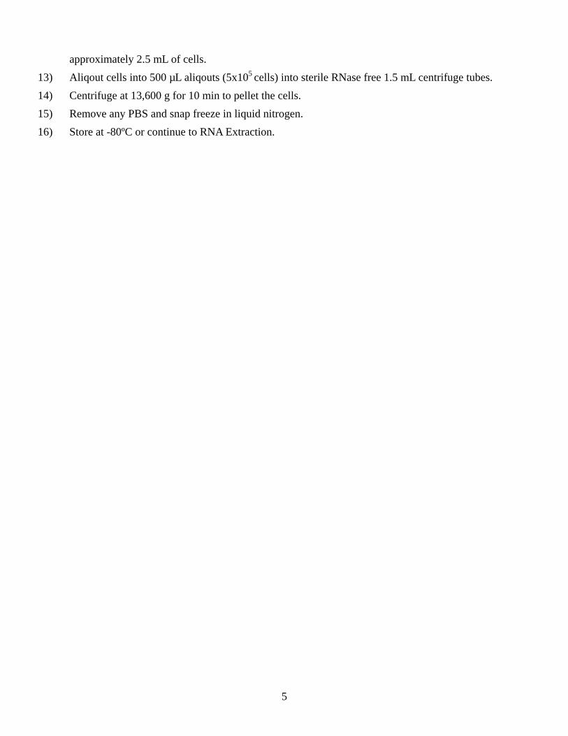
12) The above calculation will have it so that 1 mL will have 1x10⁶ cells in it. There should be
5
approximately 2.5 mL of cells. 13) Aliqout cells into 500 µL aliqouts (5x10⁵ cells) into sterile RNase free 1.5 mL centrifuge tubes. 14) Centrifuge at 13,600 g for 10 min to pellet the cells. 15) Remove any PBS and snap freeze in liquid nitrogen. 16) Store at -80ºC or continue to RNA Extraction.
6
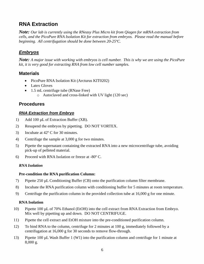
RNA Extraction Note: Our lab is currently using the RNeasy Plus Micro kit from Qiagen for mRNA extraction from cells, and the PicoPure RNA Isolation Kit for extraction from embryos. Please read the manual before beginning. All centrifugation should be done between 20-25ºC.
Embryos Note: A major issue with working with embryos is cell number. This is why we are using the PicoPure kit, it is very good for extracting RNA from low cell number samples.
Materials • PicoPure RNA Isolation Kit (Arcturus KIT0202) • Latex Gloves • 1.5 mL centrifuge tube (RNase Free)
o Autoclaved and cross-linked with UV light (120 sec)
Procedures
RNA Extraction from Embryo 1) Add 100 µL of Extraction Buffer (XB). 2) Resupend the embryos by pipetting. DO NOT VORTEX. 3) Incubate at 42º C for 30 minutes. 4) Centrifuge the sample at 3,000 g for two minutes. 5) Pipette the supernatant containing the extracted RNA into a new microcentrifuge tube, avoiding
pick-up of pelleted material. 6) Proceed with RNA Isolation or freeze at -80º C.
RNA Isolation
Pre-condition the RNA purification Column: 7) Pipette 250 µL Conditioning Buffer (CB) onto the purification column filter membrane. 8) Incubate the RNA purification column with conditioning buffer for 5 minutes at room temperature. 9) Centrifuge the purification column in the provided collection tube at 16,000 g for one minute.
RNA Isolation 10) Pipette 100 µL of 70% Ethanol (EtOH) into the cell extract from RNA Extraction from Embryo.
Mix well by pipetting up and down. DO NOT CENTRIFUGE. 11) Pipette the cell extract and EtOH mixture into the pre-conditioned purification column. 12) To bind RNA to the column, centrifuge for 2 minutes at 100 g, immediately followed by a
centrifugation at 16,000 g for 30 seconds to remove flow-through. 13) Pipette 100 µL Wash Buffer 1 (W1) into the purification column and centrifuge for 1 minute at
8,000 g.
7
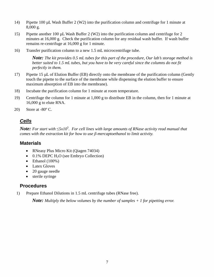
14) Pipette 100 µL Wash Buffer 2 (W2) into the purification column and centrifuge for 1 minute at 8,000 g.
15) Pipette another 100 µL Wash Buffer 2 (W2) into the purification column and centrifuge for 2 minutes at 16,000 g. Check the purification column for any residual wash buffer. If wash buffer remains re-centrifuge at 16,000 g for 1 minute.
16) Transfer purification column to a new 1.5 mL microcentrifuge tube.
Note: The kit provides 0.5 mL tubes for this part of the procedure, Our lab’s storage method is better suited to 1.5 mL tubes, but you have to be very careful since the columns do not fit perfectly in them.
17) Pipette 15 µL of Elution Buffer (EB) directly onto the membrane of the purification column (Gently touch the pipette to the surface of the membrane while dispensing the elution buffer to ensure maximum absorption of EB into the membrane).
18) Incubate the purification column for 1 minute at room temperature. 19) Centrifuge the column for 1 minute at 1,000 g to distribute EB in the column, then for 1 minute at
16,000 g to elute RNA. 20) Store at -80º C.
Cells Note: For start with ≤5x10⁵. For cell lines with large amounts of RNase activity read manual that comes with the extraction kit for how to use β-mercaptoethanol to limit activity.
Materials • RNeasy Plus Micro Kit (Qiagen 74034) • 0.1% DEPC H2O (see Embryo Collection) • Ethanol (100%) • Latex Gloves • 20 gauge needle • sterile syringe
Procedures 1) Prepare Ethanol Dilutions in 1.5 mL centrifuge tubes (RNase free).
Note: Multiply the below volumes by the number of samples + 1 for pipetting error.
8
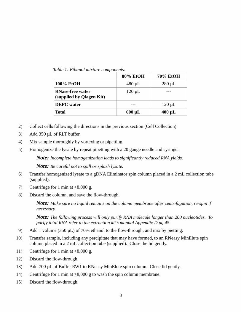
Table 1: Ethanol mixture components. 80% EtOH 70% EtOH 100% EtOH 480 µL 280 µL RNase-free water (supplied by Qiagen Kit)
120 µL ---
DEPC water --- 120 µL Total 600 µL 400 µL
2) Collect cells following the directions in the previous section (Cell Collection). 3) Add 350 µL of RLT buffer. 4) Mix sample thoroughly by vortexing or pipetting. 5) Homogenize the lysate by repeat pipetting with a 20 gauge needle and syringe.
Note: Incomplete homogenization leads to significantly reduced RNA yields.
Note: Be careful not to spill or splash lysate. 6) Transfer homogenized lysate to a gDNA Eliminator spin column placed in a 2 mL collection tube
(supplied). 7) Centrifuge for 1 min at ≥8,000 g. 8) Discard the column, and save the flow-through.
Note: Make sure no liquid remains on the column membrane after centrifugation, re-spin if necessary.
Note: The following process will only purify RNA molecule longer than 200 nucleotides. To purify total RNA refer to the extraction kit’s manual Appendix D pg 45.
9) Add 1 volume (350 µL) of 70% ethanol to the flow-through, and mix by pietting. 10) Transfer sample, including any percipitate that may have formed, to an RNeasy MinElute spin
column placed in a 2 mL collection tube (supplied). Close the lid gently. 11) Centrifuge for 1 min at ≥8,000 g. 12) Discard the flow-through. 13) Add 700 µL of Buffer RW1 to RNeasy MinElute spin column. Close lid gently. 14) Centrifuge for 1 min at ≥8,000 g to wash the spin column membrane. 15) Discard the flow-through.
9
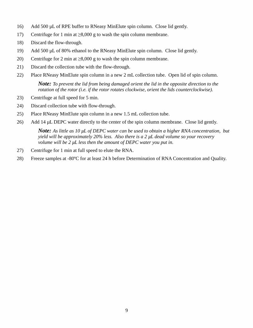
16) Add 500 µL of RPE buffer to RNeasy MinElute spin column. Close lid gently. 17) Centrifuge for 1 min at ≥8,000 g to wash the spin column membrane. 18) Discard the flow-through. 19) Add 500 µL of 80% ethanol to the RNeasy MinElute spin column. Close lid gently. 20) Centrifuge for 2 min at ≥8,000 g to wash the spin column membrane. 21) Discard the collection tube with the flow-through. 22) Place RNeasy MinElute spin column in a new 2 mL collection tube. Open lid of spin column.
Note: To prevent the lid from being damaged orient the lid in the opposite direction to the rotation of the rotor (i.e. if the rotor rotates clockwise, orient the lids counterclockwise).
23) Centrifuge at full speed for 5 min. 24) Discard collection tube with flow-through. 25) Place RNeasy MinElute spin column in a new 1.5 mL collection tube. 26) Add 14 µL DEPC water directly to the center of the spin column membrane. Close lid gently.
Note: As little as 10 µL of DEPC water can be used to obtain a higher RNA concentration, but yield will be approximately 20% less. Also there is a 2 µL dead volume so your recovery volume will be 2 µL less then the amount of DEPC water you put in.
27) Centrifuge for 1 min at full speed to elute the RNA. 28) Freeze samples at -80ºC for at least 24 h before Determination of RNA Concentration and Quality.
10
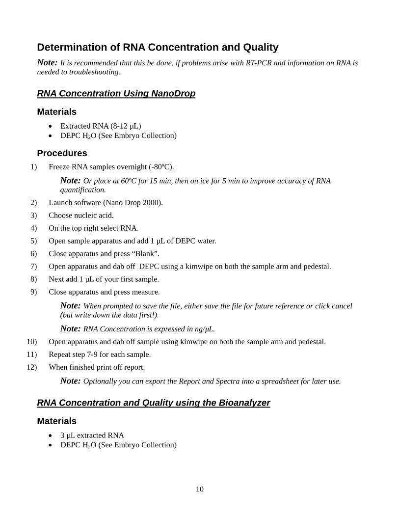
Determination of RNA Concentration and Quality Note: It is recommended that this be done, if problems arise with RT-PCR and information on RNA is needed to troubleshooting.
RNA Concentration Using NanoDrop
Materials • Extracted RNA (8-12 µL) • DEPC H2O (See Embryo Collection)
Procedures 1) Freeze RNA samples overnight (-80ºC).
Note: Or place at 60ºC for 15 min, then on ice for 5 min to improve accuracy of RNA quantification.
2) Launch software (Nano Drop 2000). 3) Choose nucleic acid. 4) On the top right select RNA. 5) Open sample apparatus and add 1 µL of DEPC water. 6) Close apparatus and press “Blank”. 7) Open apparatus and dab off DEPC using a kimwipe on both the sample arm and pedestal. 8) Next add 1 µL of your first sample. 9) Close apparatus and press measure.
Note: When prompted to save the file, either save the file for future reference or click cancel (but write down the data first!).
Note: RNA Concentration is expressed in ng/µL. 10) Open apparatus and dab off sample using kimwipe on both the sample arm and pedestal. 11) Repeat step 7-9 for each sample. 12) When finished print off report.
Note: Optionally you can export the Report and Spectra into a spreadsheet for later use.
RNA Concentration and Quality using the Bioanalyzer
Materials • 3 µL extracted RNA • DEPC H2O (See Embryo Collection)
11
Procedures 1) Freeze RNA samples overnight (-80ºC).
Note: Alternatively, place at 60ºC for 15 min, then on ice for 5 min to improve accuracy of RNA quantification.
2) Aliquot 3 µL of sample and take it to the ICBR and have them run the sample using the Pico kit.
Note: The machine measures 18S and 26S RNA. For embyros prior to embryonic genome activation, these two RNAs are very low and the Bioanalyzer would not provide a good assessment of RNA quality.
12
DNase Treatment Note: This part of the procedure is optional. It is suggested unless your primers were specifically designed around an intron to exclude amplification of DNA.
Materials • DEPC H2O (See Embryo Collection) • 12 µL of extracted RNA • DNase I Reaction (Biolabs M0303S) • 8-strip 0.2 mL tubes (Fisher 951010022)
o cross-linked with UV light (120 sec)
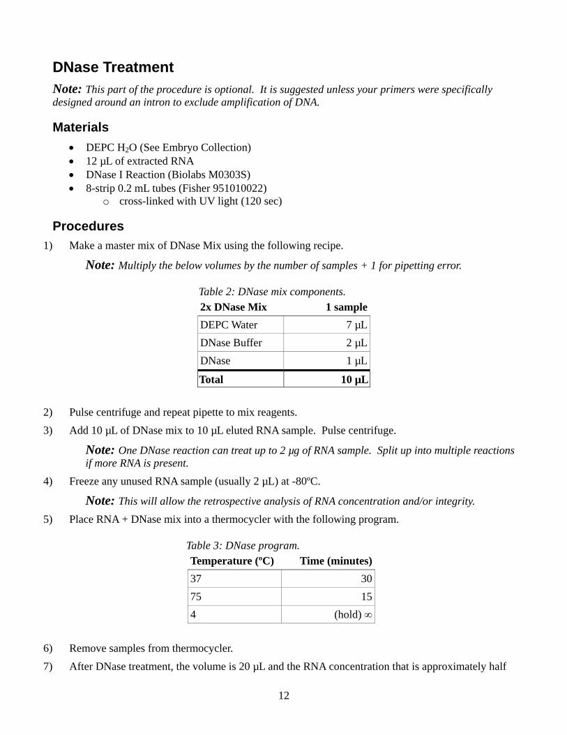
Procedures 1) Make a master mix of DNase Mix using the following recipe.
Note: Multiply the below volumes by the number of samples + 1 for pipetting error.
Table 2: DNase mix components. 2x DNase Mix 1 sampleDEPC Water 7 µLDNase Buffer 2 µLDNase 1 µL
Total 10 µL
2) Pulse centrifuge and repeat pipette to mix reagents. 3) Add 10 µL of DNase mix to 10 µL eluted RNA sample. Pulse centrifuge.
Note: One DNase reaction can treat up to 2 µg of RNA sample. Split up into multiple reactions if more RNA is present.
4) Freeze any unused RNA sample (usually 2 µL) at -80ºC.
Note: This will allow the retrospective analysis of RNA concentration and/or integrity. 5) Place RNA + DNase mix into a thermocycler with the following program.
Table 3: DNase program. Temperature (ºC) Time (minutes)37 3075 154 (hold) ∞
6) Remove samples from thermocycler. 7) After DNase treatment, the volume is 20 µL and the RNA concentration that is approximately half
13
of starting material because of dilution. 8) For embryo work, we have found it is best to add another 15 µL of DEPC H2O to the sample after
DNase treatment to bring the total volume to 35 µL. 9) Proceed to Reverse Transcription (RT) or store at -80ºC.
14
Reverse Transcription (RT) For Real-Time PCR Note: For embryo work, duplicate reactions are used for RT-PCR instead of triplicate reactions. which are used for most other samples. The reduction in replication helps conserve embryonic RNA so more primer/probe sets can be examined in individual samples. Also an additional reaction is set up lacking RTase that will serve as a negative control.
Materials • DNase Treated RNA • DEPC H2O (See Embryo Collection) • High Capacity cDNA RT (Applied Biosystems 4368814) • 8-strip 0.2 mL tubes (Fisher 951010022)
o cross-linked with UV light (120 sec)
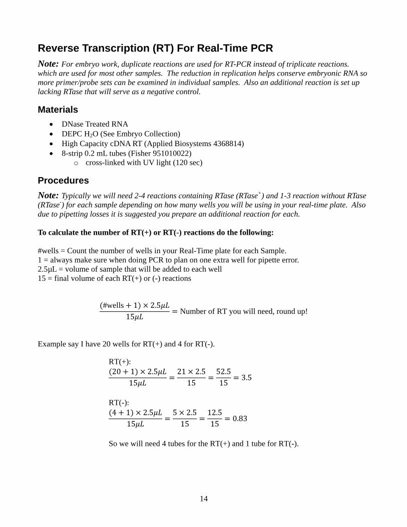
Procedures Note: Typically we will need 2-4 reactions containing RTase (RTase+) and 1-3 reaction without RTase (RTase-) for each sample depending on how many wells you will be using in your real-time plate. Also due to pipetting losses it is suggested you prepare an additional reaction for each. To calculate the number of RT(+) or RT(-) reactions do the following: #wells = Count the number of wells in your Real-Time plate for each Sample. 1 = always make sure when doing PCR to plan on one extra well for pipette error. 2.5µL = volume of sample that will be added to each well 15 = final volume of each RT(+) or (-) reactions
#wells 1 2.515 Number of RT you will need, round up!
Example say I have 20 wells for RT(+) and 4 for RT(-).
RT(+):20 1 2.5
1521 2.5
1552.515 3.5
RT(-):4 1 2.5
155 2.5
1512.515 0.83
So we will need 4 tubes for the RT(+) and 1 tube for RT(-).
15
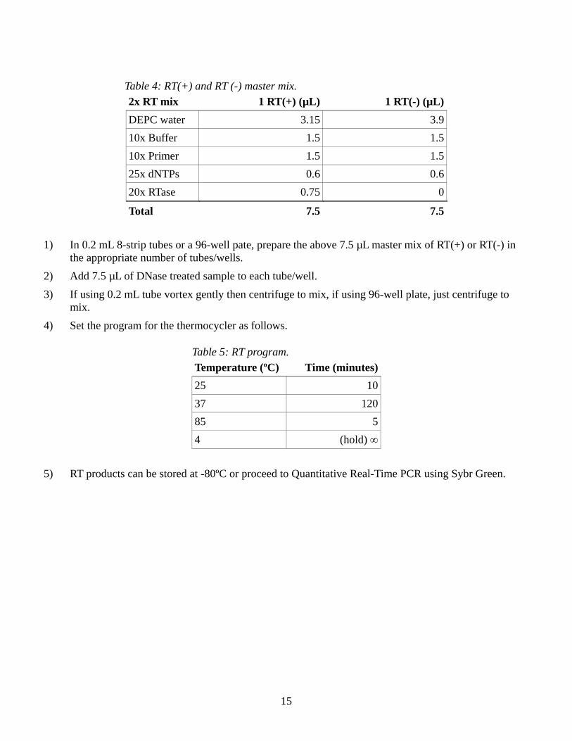
Table 4: RT(+) and RT (-) master mix. 2x RT mix 1 RT(+) (µL) 1 RT(-) (µL) DEPC water 3.15 3.9 10x Buffer 1.5 1.5 10x Primer 1.5 1.5 25x dNTPs 0.6 0.6 20x RTase 0.75 0
Total 7.5 7.5
1) In 0.2 mL 8-strip tubes or a 96-well pate, prepare the above 7.5 µL master mix of RT(+) or RT(-) in the appropriate number of tubes/wells.
2) Add 7.5 µL of DNase treated sample to each tube/well. 3) If using 0.2 mL tube vortex gently then centrifuge to mix, if using 96-well plate, just centrifuge to
mix. 4) Set the program for the thermocycler as follows.
Table 5: RT program. Temperature (ºC) Time (minutes)25 1037 12085 54 (hold) ∞
5) RT products can be stored at -80ºC or proceed to Quantitative Real-Time PCR using Sybr Green.
Npscr ipw
TFwr
Quantita
Running Note: Befoproperly (prstandard RNcontaining trange (ng to
Afterinto one tubpoint in the was 300 ng/
Do aTime plate +From the prewells each. Trounded up t
ative Re
a Standare using new
rimer efficienNA sample (ithe transcripo pg/fg conce
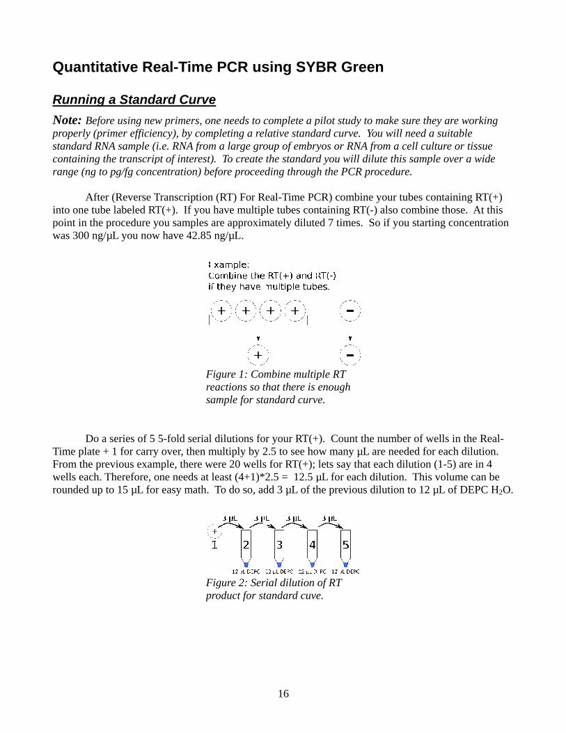
r (Reverse Te labeled RTprocedure y
/µL you now
a series of 5 5+ 1 for carry evious examTherefore, oto 15 µL for
eal-Time
ard Curvew primers, onncy), by comi.e. RNA frompt of interest)entration) be
TranscriptionT(+). If you ou samples a
w have 42.85
5-fold serialover, then m
mple, there wone needs at r easy math.
Fpr
Fresa
e PCR us
e ne needs to c
mpleting a relm a large gro). To create efore procee
n (RT) For Rhave multipare approximng/µL.
dilutions fomultiply by 2
were 20 wellsleast (4+1)* To do so, ad
Figure 2: Serroduct for st
Figure 1: Comeactions so tample for sta
16
sing SYB
complete a plative standaoup of embrythe standardding through
Real-Time PCple tubes conmately dilute
or your RT(+2.5 to see hos for RT(+); 2.5 = 12.5 µdd 3 µL of th
rial dilution otandard cuve
mbine multipthat there is andard curv
BR Gree
pilot study toard curve. Yyos or RNA fd you will dih the PCR pr
CR) combinentaining RT(-ed 7 times. S
+). Count theow many µL lets say thatµL for each dhe previous d
of RT e.
ple RT enough e.
en
o make sure tYou will needfrom a cell cilute this samrocedure.
e your tubes -) also combSo if you sta
e number of are needed f
t each dilutiodilution. Thdilution to 1
they are word a suitable culture or tismple over a w
containing Rbine those. Aarting concen
f wells in thefor each diluon (1-5) are ihis volume ca2 µL of DEP
rking
ssue wide
RT(+) At this ntration
e Real-ution. in 4 an be PC H2O.
17
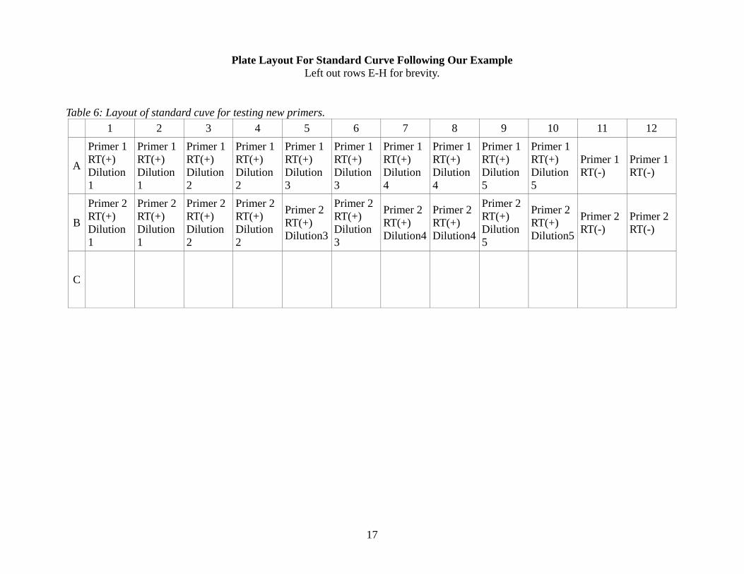
Plate Layout For Standard Curve Following Our Example Left out rows E-H for brevity.
Table 6: Layout of standard cuve for testing new primers. 1 2 3 4 5 6 7 8 9 10 11 12
A
Primer 1 RT(+) Dilution 1
Primer 1 RT(+) Dilution 1
Primer 1 RT(+) Dilution 2
Primer 1 RT(+) Dilution 2
Primer 1 RT(+) Dilution 3
Primer 1 RT(+) Dilution 3
Primer 1 RT(+) Dilution 4
Primer 1 RT(+) Dilution 4
Primer 1 RT(+) Dilution 5
Primer 1 RT(+) Dilution 5
Primer 1 RT(-)
Primer 1 RT(-)
B
Primer 2 RT(+) Dilution 1
Primer 2 RT(+) Dilution 1
Primer 2 RT(+) Dilution 2
Primer 2 RT(+) Dilution 2
Primer 2 RT(+) Dilution3
Primer 2 RT(+) Dilution 3
Primer 2 RT(+) Dilution4
Primer 2 RT(+) Dilution4
Primer 2 RT(+) Dilution 5
Primer 2 RT(+) Dilution5
Primer 2 RT(-)
Primer 2 RT(-)
C
18
Materials • Diluted Forward and Reverse Primers (see Primer Dilution) • SYBR Green (Applied Biosystems 4309155) • Real-Time PCR 96-well Plate (Applied Biosystems 4306737) • Real-Time PCR Film for 96-well Plate (Applied Biosystems 4311971) • 1.5 mL centrifuge tube (RNase Free)
o Autoclaved and cross-linked with UV light (120 sec) • 8-strip 0.2 mL tubes (Fisher 951010022)
o cross-linked with UV light (120 sec)
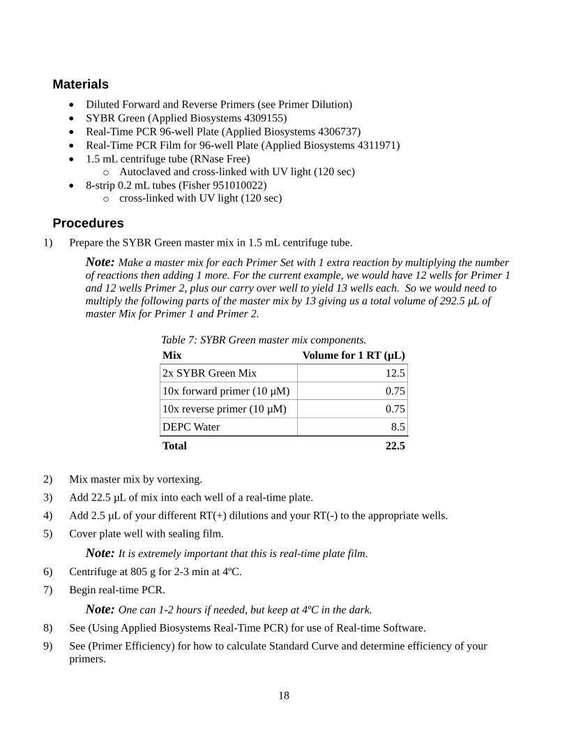
Procedures 1) Prepare the SYBR Green master mix in 1.5 mL centrifuge tube.
Note: Make a master mix for each Primer Set with 1 extra reaction by multiplying the number of reactions then adding 1 more. For the current example, we would have 12 wells for Primer 1 and 12 wells Primer 2, plus our carry over well to yield 13 wells each. So we would need to multiply the following parts of the master mix by 13 giving us a total volume of 292.5 µL of master Mix for Primer 1 and Primer 2.
Table 7: SYBR Green master mix components. Mix Volume for 1 RT (µL) 2x SYBR Green Mix 12.5 10x forward primer (10 µM) 0.75 10x reverse primer (10 µM) 0.75 DEPC Water 8.5
Total 22.5
2) Mix master mix by vortexing. 3) Add 22.5 µL of mix into each well of a real-time plate. 4) Add 2.5 µL of your different RT(+) dilutions and your RT(-) to the appropriate wells. 5) Cover plate well with sealing film.
Note: It is extremely important that this is real-time plate film. 6) Centrifuge at 805 g for 2-3 min at 4ºC. 7) Begin real-time PCR.
Note: One can 1-2 hours if needed, but keep at 4ºC in the dark. 8) See (Using Applied Biosystems Real-Time PCR) for use of Real-time Software. 9) See (Primer Efficiency) for how to calculate Standard Curve and determine efficiency of your
primers.
19
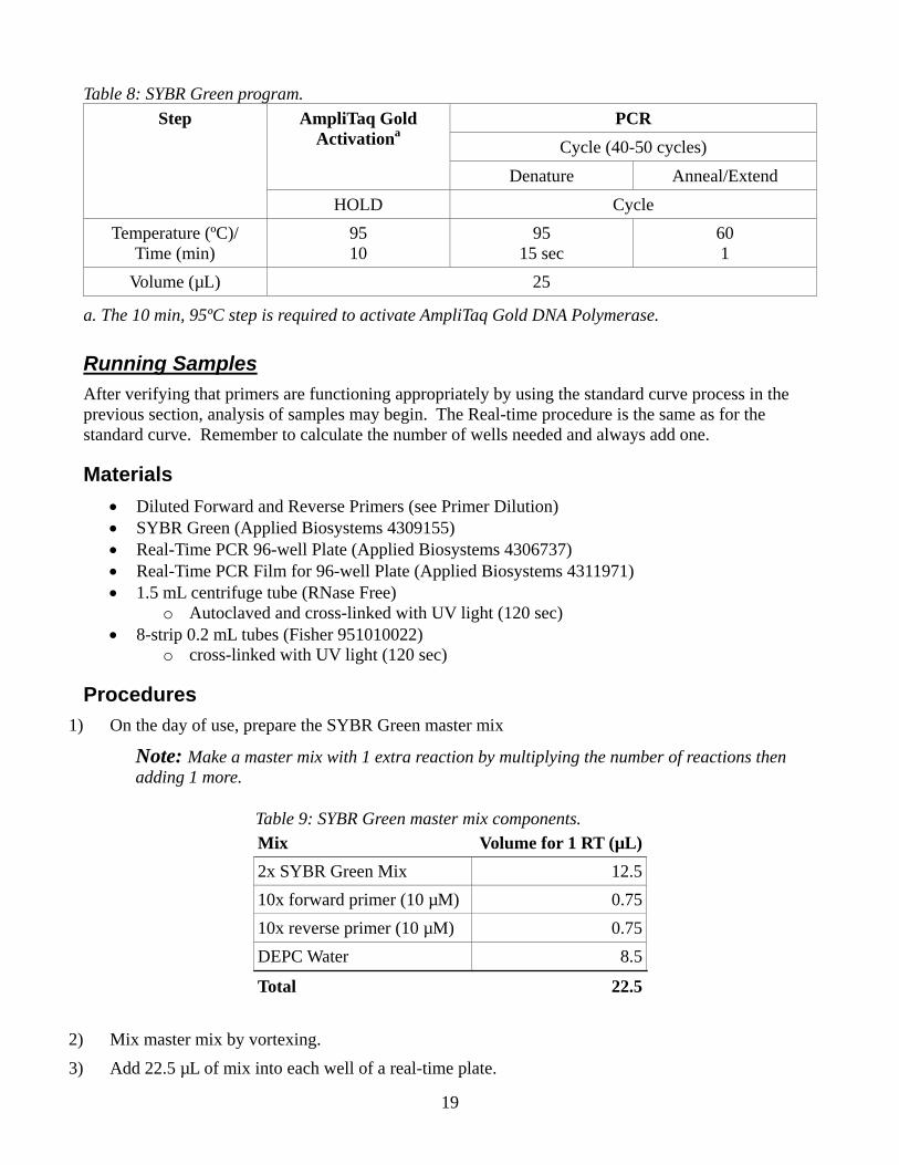
Table 8: SYBR Green program. Step AmpliTaq Gold
Activationa PCR
Cycle (40-50 cycles) Denature Anneal/Extend
HOLD Cycle Temperature (ºC)/
Time (min) 95 10
95 15 sec
60 1
Volume (µL) 25
a. The 10 min, 95ºC step is required to activate AmpliTaq Gold DNA Polymerase.
Running Samples After verifying that primers are functioning appropriately by using the standard curve process in the previous section, analysis of samples may begin. The Real-time procedure is the same as for the standard curve. Remember to calculate the number of wells needed and always add one.
Materials • Diluted Forward and Reverse Primers (see Primer Dilution) • SYBR Green (Applied Biosystems 4309155) • Real-Time PCR 96-well Plate (Applied Biosystems 4306737) • Real-Time PCR Film for 96-well Plate (Applied Biosystems 4311971) • 1.5 mL centrifuge tube (RNase Free)
o Autoclaved and cross-linked with UV light (120 sec) • 8-strip 0.2 mL tubes (Fisher 951010022)
o cross-linked with UV light (120 sec)
Procedures 1) On the day of use, prepare the SYBR Green master mix
Note: Make a master mix with 1 extra reaction by multiplying the number of reactions then adding 1 more.
Table 9: SYBR Green master mix components. Mix Volume for 1 RT (µL) 2x SYBR Green Mix 12.5 10x forward primer (10 µM) 0.75 10x reverse primer (10 µM) 0.75 DEPC Water 8.5
Total 22.5
2) Mix master mix by vortexing. 3) Add 22.5 µL of mix into each well of a real-time plate.
20
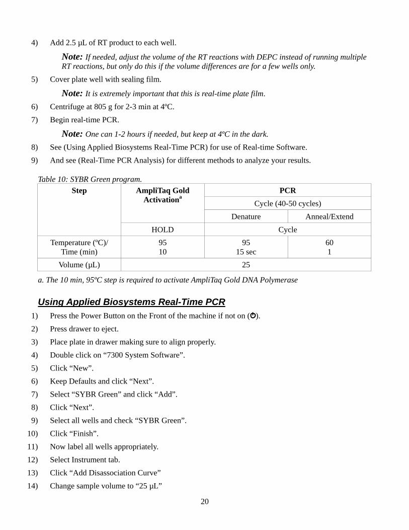
4) Add 2.5 µL of RT product to each well.
Note: If needed, adjust the volume of the RT reactions with DEPC instead of running multiple RT reactions, but only do this if the volume differences are for a few wells only.
5) Cover plate well with sealing film.
Note: It is extremely important that this is real-time plate film. 6) Centrifuge at 805 g for 2-3 min at 4ºC. 7) Begin real-time PCR.
Note: One can 1-2 hours if needed, but keep at 4ºC in the dark. 8) See (Using Applied Biosystems Real-Time PCR) for use of Real-time Software. 9) And see (Real-Time PCR Analysis) for different methods to analyze your results.
Table 10: SYBR Green program. Step AmpliTaq Gold
Activationa PCR
Cycle (40-50 cycles) Denature Anneal/Extend
HOLD Cycle Temperature (ºC)/
Time (min) 95 10
95 15 sec
60 1
Volume (µL) 25
a. The 10 min, 95ºC step is required to activate AmpliTaq Gold DNA Polymerase
Using Applied Biosystems Real-Time PCR 1) Press the Power Button on the Front of the machine if not on ( ). 2) Press drawer to eject. 3) Place plate in drawer making sure to align properly. 4) Double click on “7300 System Software”. 5) Click “New”. 6) Keep Defaults and click “Next”. 7) Select “SYBR Green” and click “Add”. 8) Click “Next”. 9) Select all wells and check “SYBR Green”.
10) Click “Finish”. 11) Now label all wells appropriately. 12) Select Instrument tab. 13) Click “Add Disassociation Curve” 14) Change sample volume to “25 µL”

21
15) File >> Save... [C:\Applied Biosystems\SDSDocument\USERNAME\*.sds]. 16) Click “Start”. 17) When Finished Click “OK”. 18) Press the(►) to Analyze. 19) File >> Export Results...
22
End Point PCR
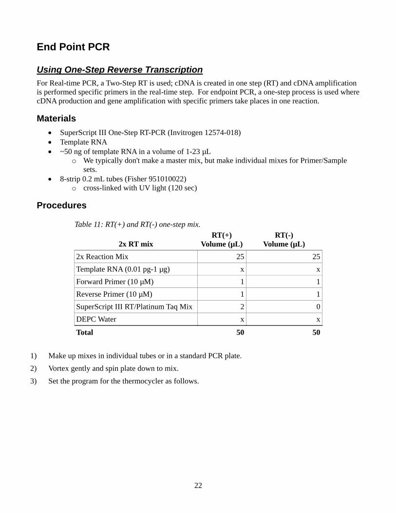
Using One-Step Reverse Transcription For Real-time PCR, a Two-Step RT is used; cDNA is created in one step (RT) and cDNA amplification is performed specific primers in the real-time step. For endpoint PCR, a one-step process is used where cDNA production and gene amplification with specific primers take places in one reaction.
Materials • SuperScript III One-Step RT-PCR (Invitrogen 12574-018) • Template RNA • ~50 ng of template RNA in a volume of 1-23 µL
o We typically don't make a master mix, but make individual mixes for Primer/Sample sets.
• 8-strip 0.2 mL tubes (Fisher 951010022) o cross-linked with UV light (120 sec)
Procedures
Table 11: RT(+) and RT(-) one-step mix.
2x RT mix RT(+)
Volume (µL)RT(-)
Volume (µL) 2x Reaction Mix 25 25Template RNA (0.01 pg-1 µg) x xForward Primer (10 µM) 1 1Reverse Primer (10 µM) 1 1SuperScript III RT/Platinum Taq Mix 2 0DEPC Water x x
Total 50 50
1) Make up mixes in individual tubes or in a standard PCR plate. 2) Vortex gently and spin plate down to mix. 3) Set the program for the thermocycler as follows.
23
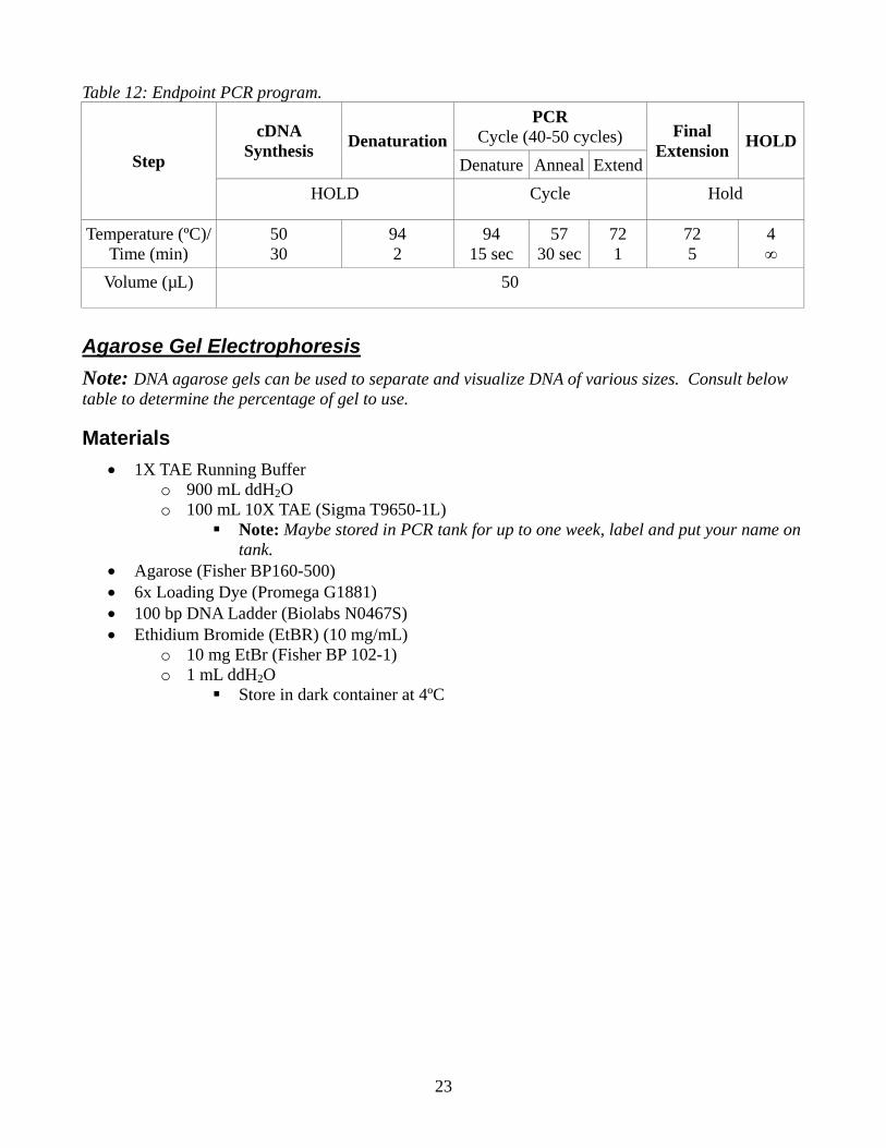
Table 12: Endpoint PCR program.
Step
cDNA Synthesis Denaturation
PCR Cycle (40-50 cycles) Final
Extension HOLDDenature Anneal Extend
HOLD Cycle Hold
Temperature (ºC)/ Time (min)
50 30
94 2
94 15 sec
57 30 sec
72 1
72 5
4 ∞
Volume (µL) 50
Agarose Gel Electrophoresis Note: DNA agarose gels can be used to separate and visualize DNA of various sizes. Consult below table to determine the percentage of gel to use.
Materials • 1X TAE Running Buffer
o 900 mL ddH2O o 100 mL 10X TAE (Sigma T9650-1L)
Note: Maybe stored in PCR tank for up to one week, label and put your name on tank.
• Agarose (Fisher BP160-500) • 6x Loading Dye (Promega G1881) • 100 bp DNA Ladder (Biolabs N0467S) • Ethidium Bromide (EtBR) (10 mg/mL)
o 10 mg EtBr (Fisher BP 102-1) o 1 mL ddH2O
Store in dark container at 4ºC
24
Procedures
Casting Gel
Table 13: Suggest gel concentrations for different product sizes. Gel Concentration (%) DNA Product Size (Kb) 0.5 1-30 0.75 0.8-12 1 0.5-10 1.25 0.4-7 1.5 0.2-3 2-5 0.01-0.5
Table 14: Components for different gel concentrations. 0.7% 1% 2% 3% 4% Agarose 0.7 g 1.0 g 2.0 g 3.0 g 4.0g 20X TAE 10 mL 10 mL 10 mL 10 mL 10 mL DEPC Water 90 mL 90 mL 90 mL 90 mL 90 mL EtBr (10mg/mL) 10 µL 10 µL 10 µL 10 µL 10 µL Total vol 100 mL 100 mL 100 mL 100 mL 100 mL
1) Combine the needed amount of agarose, TAE, and DEPC water in a 250 mL Erlenmeyer flask. 2) Swirl to suspend agarose. 3) Place the gel solution into the microwave. Microwave for 2-3 min. 4) This will bring the solution to a boil. 5) Carefully swirl to mix and make sure all agarose is dissolved, if not microwave for 30 sec until
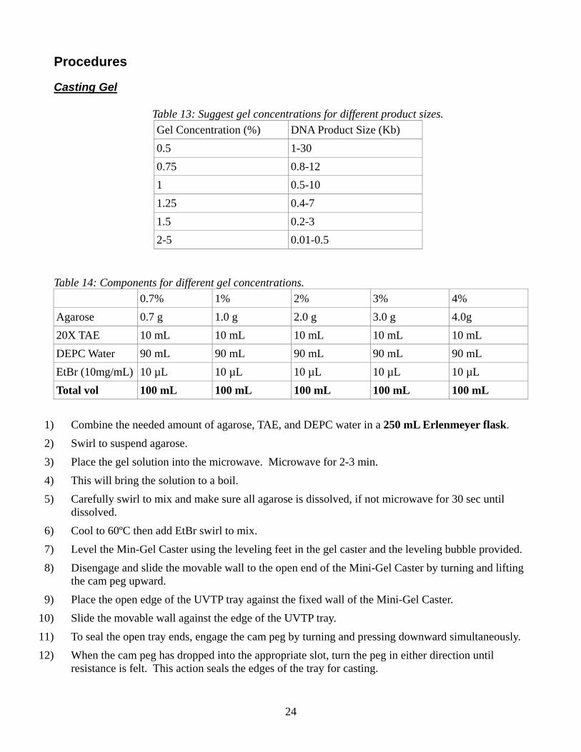
dissolved. 6) Cool to 60ºC then add EtBr swirl to mix. 7) Level the Min-Gel Caster using the leveling feet in the gel caster and the leveling bubble provided. 8) Disengage and slide the movable wall to the open end of the Mini-Gel Caster by turning and lifting
the cam peg upward. 9) Place the open edge of the UVTP tray against the fixed wall of the Mini-Gel Caster.
10) Slide the movable wall against the edge of the UVTP tray. 11) To seal the open tray ends, engage the cam peg by turning and pressing downward simultaneously. 12) When the cam peg has dropped into the appropriate slot, turn the peg in either direction until
resistance is felt. This action seals the edges of the tray for casting.
25
13) Place the comb(s) into the appropriate slot(s) of the tray. 14) When agarose has cooled to 50-60ºC pour the molten agarose between the gates. 15) Allow 20-40 min for the gel to solidify at room temperature. 16) Carefully remove the comb from the solidified gel. 17) Disengage the cam peg by turning and lifting upward. Slide the movable wall wall away from the
tray. Remove the tray from the Mini-Gel Caster. 18) Place the tray onto the leveled Sub-Cell base so the sample wells are near the cathode (black). DNA
samples will migrate toward the anode (red) during electrophoresis. 19) Submerge the gel beneath 2 to 6 mm of 1x electrophoresis buffer.
Note: User a greater depth overlay when using higher voltages to avoid pH and heat effects.
Sample Preparation 20) Bleach a piece of parafilm by spraying with 10% Bleach solution and wipe dry with kimwipe. 21) Place a 2 µL drop of loading buffer for each lane that will have sample on the parafilm. 22) Mix 10 µL of sample with 2 µL of loading buffer by repeat pipetting. 23) Place 10 µL of sample + loading buffer in each lane. 24) Place 6 µL of ladder in the first lane.
Note: You may also want to add ladder to the last lane. 25) Run gel Black to Red (70 V/160 mA) for about 1 h. 26) After about 1 h check the progress of the gel by stopping running and looking at the gel under UV
light. Do this until you have the separation you are wanting.
26
27) Take picture of the gel.
Note: Remember to bleach all surfaces that the gel comes in contact with, to prevent EtBr residue from being left behind.
28) Place gel in a 10% Bleach solution overnight to neutralize any EtBr in the gel, then dispose of appropriately.
27
Acknowledgments This set of protocols is the culmination of protocols from several labs, internet resources, and manufacturer’s product inserts that have been adapted to fit our needs. The majority of PCR tasks today can be accomplished by the purchase of a simple kit. It is recommended that the manufacturer’s guidelines are read and understood. The majority of the above protocols were adapted from such guidelines. Below are a list of references that helped in not only in the development of the above protocols, but also in the development of our understanding of PCR. We would like to give special thanks to Dr. Manabu Ozawa for his help and guidance.
References Easton, D., 2008. BIO450 Primer Design Tutorial. Buffalo State. http://faculty.buffalostate.edu/eastondp/dpeastonbiolog/Bio%20450/BIO450%20Primer%20Design%20Tutorial%202008.pdf Hunt, M., 2009. Real Time PCR. University of South Carolina School of Medicine. http://pathmicro.med.sc.edu/pcr/realtime-home.htm Moore, K. 2008. Moore Lab Protocol: Designing PCR Primers. University of Florida. Pennington, K., et al. 2009. Ealy Lab Protocol: Suggestions for Using SYBR Green qRT-PCR when Quantifying mRNA from Bovine Embryos. University of Florida. Poole, D H., 2009. Pate Lab Protocol: Polymerase Chain Reaction. Penn State University. Szick-Miranda, K., 2009. BIO430 Primer Design. CSU-Bakersfield. http://www.csub.edu/~kszick_miranda/Primer%20Design.doc
28
Appendix
Other Reagents
General • 100 mM Sodium Phosphate Monobaisc (NaH2PO4•2H2O)
o 13.8 g NaH2PO4 (Sigma S9638-250G) o 1 L ddH2O
• 100 mM Sodium Phosphate Dibasic (Na2HPO4) o 14.2 g Na2HPO4•2H2O (Sigma S0876-1KG) o 1 L ddH2O
• 0.1 M PBS (pH 7.4) o 100 mL 100mM Sodium Phosphate Monobaisc o ~300 mL 100mM Sodium Phosphate Dibasic
Add only enough to reach a pH of 7.4 • PBS + NaCl
o 100 mL 0.1M PBS o 900 mL ddH2O o 9g NaCl (Sigma S7653-1KG)
• Protease (0.1%) (aka pronase) o 0.1 g Protease (P8811-1G) from Streptomyces griseus o 100 mL 0.1M PBS
Note filtering here will prevent particulate from being in aliqouts Make 1 mL aliquots and freeze at -20ºC
• Alternative: Protease 0.5% o 0.5 g Protease (P8811-1G) from Streptomyces griseus o 100 mL 0.1 M PBS o Make 1 mL aliqouts and freeze at -20ºC
Electrophoresis • 50X TAE
o 242 g Tris Base o 57.1 mL Glacial Acetic Acid o 100 mL 0.5 M EDTA pH 7.8 o 842.9 mL ddH2O
• Loading Dye o 0.25 g Bromophenal Blue o 0.25 g Xylene cyanol o 50 mL Glycerol o 1 mL 1 M Tris o 100 mL ddH2O
N Aht
WI
c
tcc Hdtc M
Using a HNote: Mod
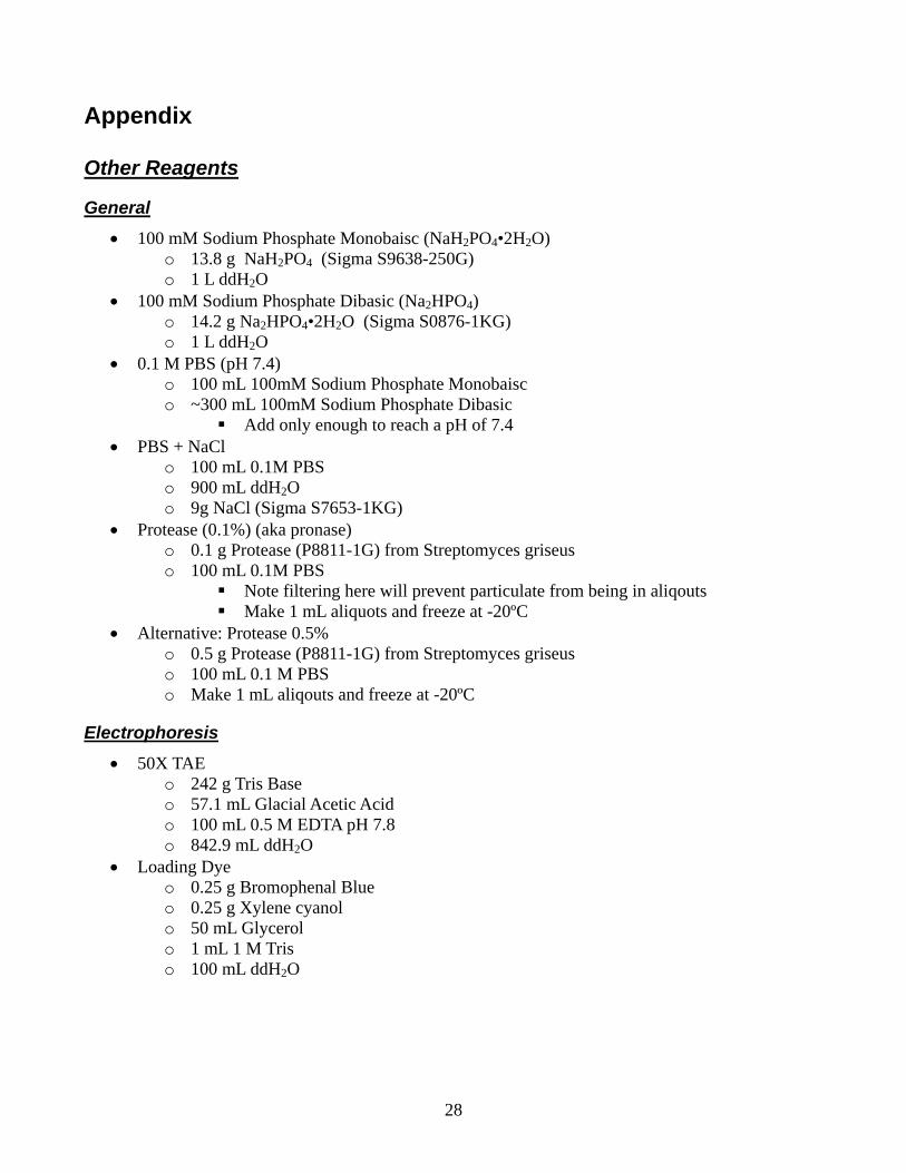
A hemacytohold a quartztotal surface
Calculation W in FigureIn both methsuspended mcontents so t
Staining of ctrypan blue cells with 10cells.
Here are twodetermine cethe cell conccell concent
Method A:
Hemocytodified from th
meter (also z coverslip e
e area of 9 m
of concentra 5) has a volhods, the hemmix of cells athat the fluid
cells often fa[0.4% (w/v)0% formalin
o simple metell count. Otcentration - ttration is low
Count the nu
ometer he Hansen La
spelled hemexactly 0.1 m
mm2 Figure 4
ation is baselume of 0.00mocytometeat the notch d is drawn in
acilitates vis) tyrypan blun and then sta
thods for couther countingthe accuracy
w, one should
umber of cel
Figur
ab Protocol
ocytometer)mm above th4.
d on the volu001 ml (lengr is filled byat the edge o
nto the cham
ualization anue in PBS] toain with tryp
unting cells g schemes ary of the proced count more
lls in the 4 o
re 4: Dimens
29
by P. J. Han
) is an etchedhe chamber f
ume undernegth x width xy capillary acof the hemoc
mber by capil
nd counting.o determine lpan blue or o
based on there accetable edure depene grids.
outer squares
sions of a he
nsen
d glass chamfloor. The co
eath the covx height; i.e.,ction - place cytometer anllary action.
. Either mixlive/dead coother stain (t
e surface arealso. The ch
nds upon the
s (see the lef
emacytomete
mber with raiounting cham
ver slip. One, 0.1 cm x 0.the pipette f
nd then slow
x cells with aount (dead ceo improve v
ea of the hemhoice of metnumber of c
ft panel of Fi
er.
sed sides thamber is etche
e large squar1 cm x 0.01 filled with a
wly expel som
an equal voluells are blue)visualization
macytometerthods depencells counted
igure 5). The
at will ed in a
re (see cm). well-
me
ume of ) or kill of all
r used to ds upon d. When
e cell
c
Mp
F
Plbrc
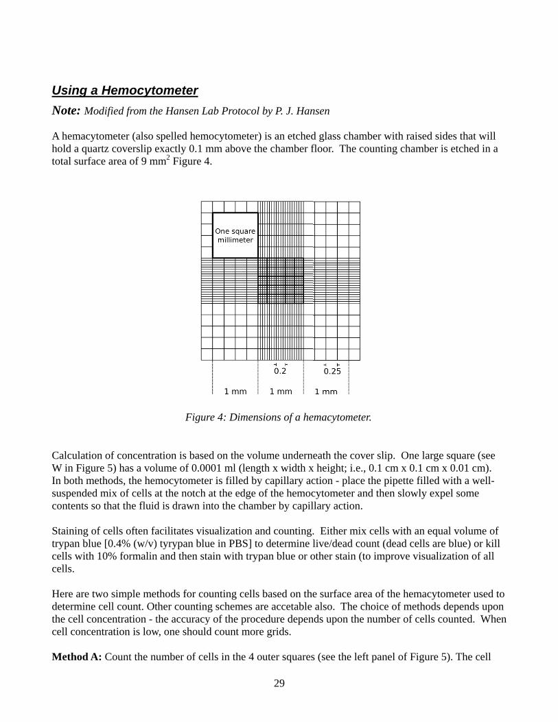
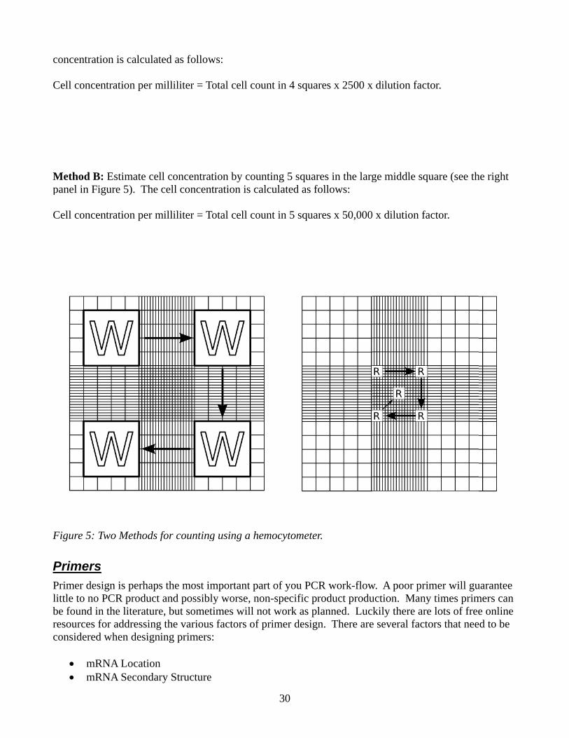
concentratio
Cell concent
Method B: panel in Figu
Cell concent
Figure 5: Tw
Primers Primer desiglittle to no Pbe found in resources foconsidered w
• mRN• mRN
on is calculat
tration per m
Estimate celure 5). The
tration per m
wo Methods f
gn is perhapsPCR product the literature
or addressingwhen design
NA LocationNA Secondar
ted as follow
milliliter = To
ll concentratcell concent
milliliter = To
for counting
s the most imand possibl
e, but sometig the variousning primers:
n ry Structure
ws:
otal cell cou
tion by countration is cal
otal cell cou
g using a hem
mportant pary worse, nonimes will no
s factors of p:
30
unt in 4 squar
nting 5 squarlculated as fo
unt in 5 squar
mocytometer
rt of you PCRn-specific prot work as plprimer design
res x 2500 x
res in the largollows:
res x 50,000
r.
R work-flowroduct produlanned. Lucn. There are
x dilution fac
ge middle sq
x dilution fa
w. A poor pruction. Manykily there ar
e several fact
ctor.
quare (see th
factor.
imer will guy times prim
re lots of freetors that nee
he right
uarantee mers can e online d to be
31
• Specificity • Primer Length • Product Size • Primer Dimers and Secondary Structure • Melting Temperature (Tm) • G/C content • G/C clamp
mRNA Location Most companies suggest that forward and reverse primers are designed so that sequences that are on different exons of a gene. This precaution makes accidental amplification of genomic DNA unlikely due to product size limitations. Treating samples with DNase makes such an accident less likely.
mRNA Secondary Structure In solution, single stranded mRNA forms secondary structure of loops and hairpins. Primers can not bind in these spots of high secondary structure. After annealing, however, extension through secondary structure is possible. When designing primers, it is important to exclude regions of high secondary structure at the annealing temperature (usually 60ºC).
Specificity PCR is capable of amplifying single target cDNA sequence from a mix of cDNA fragments. This depends on specific primers. The forward and reverse primer flank a target sequence of interest on opposite strands. A well designed primer will only bind to this cDNA fragment and amplify only the intended sequence. For this reason primers should not consist of repetitive sequences that could be commonly found in other cDNA fragments. It is also useful to blast search putative primer sequences to ensure that they do not hybridize to other genes not of interest.
Primer Length Primer length is related to specificity and annealing efficiency. Primer length considerations fit the Goldilocks paradox; they must not be too short or too long. If the primer is too short it will lack specificity and amplify other sequences. For example there is a ¼ chance of finding an A, T, G, C in any given sequence. Therefore there is a 1/16 chance of finding any di-nucleotide (e.g. AG); and a 1/256 chance of finding a 4-base sequence. Following this logic a 16 base sequence would have a 1/4,294,976,296; which is about the size of the human genome. So if your primer is 16+ bases long statistically speaking it should only be found no more then once in the genome (except it will be more common because of gene duplication). If a primer is too long, annealing efficiency will decrease because Tm is related to the primer length. It is recommended that primers for standard PCR be between 18-24 oligonucleotides in length.
Product Size Another important consideration is the length of your PCR product (i.e. the distance between your forward and reverse primer). Again this follow the Goldilocks paradox: not too short and not too long. In general, if the product is too small (<80 bp) it is difficult to visualize on an agarose gel and can causes difficulties in Real-Time PCR. If it is >1000 bp, there are difficulties for the polymerase to amplify large sequences and amplification efficiency goes down. In general it is suggested that product
32
size be between 80 and 200 bp for real time PCR (we aim for around 120 bp) and be between 150-250 bp for endpoint PCR.
Primer Dimer and Secondary Structure Another important aspect for primer design is that the primers do not dimerize with themselves or each other, and that they do not form secondary structure such as hairpins. Both dimerization and secondary structure will remove the primer from the reaction causing a decrease in PCR product. Oligocalc (http://www.basic.northwestern.edu/biotools/oligocalc.html) is a simple internet software that can predict hairpin and primer dimers.
Melting Temperature (Tm) Tm is the temperature at which half the population of double stranded molecules are in a single stranded form (i.e. the temperature at which ½ your primer annealed to the template sequence). The annealing temperature is 5ºC below Tm. The Tm can be calculated in a variety of ways:
The Wallace Rule:2 4
Sum of A and T residuesSum of C and G residues
Nearest Neighbor model:
273.15 16.6log +
Thankfully primer design software will do this for you. Typically it is suggested that Tm be between 55-80ºC with 60ºC as the optimum.
G/C Content Looking at the Wallace rule above, it is clear that G/C content has a major influence on melting temperature because G/C pairs are more stable then A/T paris, because they have a triple hydorgen bond between opposite nucleotides compared to the double hydorgen bond of A/T pairs. It is suggested that when you design a primer you aim for 50% G/C and 50% A/T. Also because of the extra stability one should avoid long runs of G/C in their primer design because this may promote mis-annealing.
G/C Clamp Similar to G/C content another important factor is the G/C clamp. It is commonly suggested that there is the presence of 1-3 G/C nucleotides in the last 5 bases of the 3' end, this will promote specific binding and initiation of polymerization. However, if you have more then 3 G/C pairs you run the risk of mis-priming.
33
Primer Design
Materials • Software
o Mfold (http://mfold.bioinfo.rpi.edu/cgi-bin/dna-form1.cgi) o Primer3/Primer3Plus (http://www.bioinformatics.nl/cgi-
bin/primer3plus/primer3plus.cgi) o BLAST (http://blast.ncbi.nlm.nih.gov/Blast.cgi) o Oligocalc (http://www.basic.northwestern.edu/biotools/oligocalc.html)
• Complete Coding Sequence for target gene in FASTA format. o Pubmed (http://www.ncbi.nlm.nih.gov/sites/entrez?db=pubmed) o GeneBank (http://www.ncbi.nlm.nih.gov/Genbank/) o EMBL (http://www.ebi.ac.uk/embl/)
Procedures 1) The first step of primer design is to obtain the sequence of your target gene using GenBank or
EMBL. Selection of the proper sequence is important, but is highly dependent on your target gene. For example if there are splice variants that you are targeting then that needs to be taken in account. In general you can either design your primers in two different exons (DNA), or using the complete coding sequence (CDS) (mRNA). If you are using the CDS then make sure to treat samples with Dnase prior to RT-PCR.
2) Download sequence in FASTA format. 3) To test for secondary structure load sequence into mfold. (http://mfold.bioinfo.rpi.edu/cgi-bin/dna-
form1.cgi). We will be using the DNA calculator given that during the PCR reaction the cDNA will be double stranded.
Note: There is a size limit for using the online version of mfold. If your target sequence is too large for the online tool then you can download and install UNA-Fold. (http://dinamelt.bioinfo.rpi.edu/download.php)
4) Adjust the settings to the PCR reaction you are going to use. Bellow are typical settings. i. The DNA sequence is “Linear”
ii. Folding temperature “60” iii. Ionic conditions: [Na+] “50” [Mg++] “2.0” iv. Units “mM” v. Leave everything else with the default settings...
vi. We normally set base numbering frequency “10” but not essential. 5) Click “Fold DNA” 6) Below is typical output from mfold
34
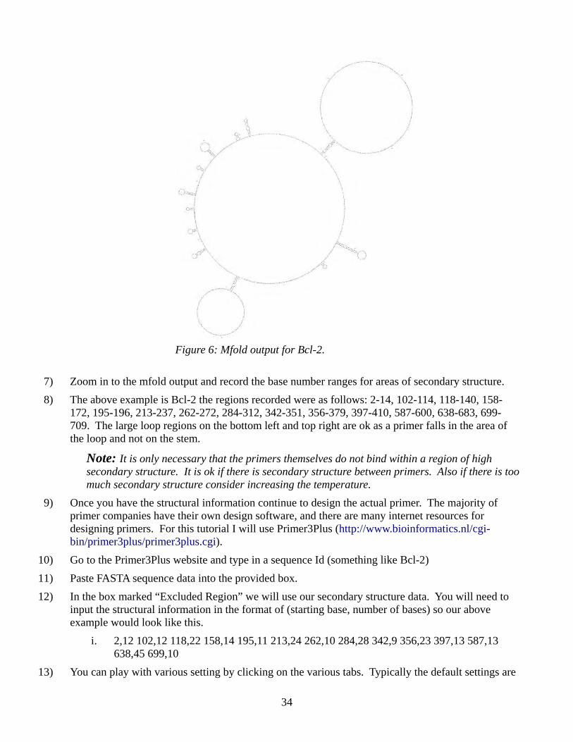
7) Zoom in to the mfold output and record the base number ranges for areas of secondary structure. 8) The above example is Bcl-2 the regions recorded were as follows: 2-14, 102-114, 118-140, 158-
172, 195-196, 213-237, 262-272, 284-312, 342-351, 356-379, 397-410, 587-600, 638-683, 699-709. The large loop regions on the bottom left and top right are ok as a primer falls in the area of the loop and not on the stem.
Note: It is only necessary that the primers themselves do not bind within a region of high secondary structure. It is ok if there is secondary structure between primers. Also if there is too much secondary structure consider increasing the temperature.
9) Once you have the structural information continue to design the actual primer. The majority of primer companies have their own design software, and there are many internet resources for designing primers. For this tutorial I will use Primer3Plus (http://www.bioinformatics.nl/cgi-bin/primer3plus/primer3plus.cgi).
10) Go to the Primer3Plus website and type in a sequence Id (something like Bcl-2) 11) Paste FASTA sequence data into the provided box. 12) In the box marked “Excluded Region” we will use our secondary structure data. You will need to
input the structural information in the format of (starting base, number of bases) so our above example would look like this.
i. 2,12 102,12 118,22 158,14 195,11 213,24 262,10 284,28 342,9 356,23 397,13 587,13 638,45 699,10
13) You can play with various setting by clicking on the various tabs. Typically the default settings are
Figure 6: Mfold output for Bcl-2.
35
fine.
Note: For real-time PCR it is suggested to adjust the product size range to 80-200. To do this click on the “General Settings” tab and change the first “Product Size Ranges” from “150-200” to “80-200”. Also it easier to output more primer pairs then the default setting (5). To change this go to the “Advanced Settings” tab and change “Number to Return” from “5” to “10”.
14) Once finished changing settings click the green box labeled “Pick Primers” on the top right. 15) The output from primer3Plus will have a list of primer pairs, in a ranked order (i.e. the primer pair
they consider best is #1 for the parameters set). 16) Select at least 3 primer sets that fit our criteria (i.e. product size, Tm, G/C content, location, etc.) by
checking the boxes next to their names then clicking “Send to Primer3Manager” 17) Once in the primer3Manager check each primer for self-complementary and secondary structure
using “Check!” and for specificity using “BLAST!”. 18) Start by checking for self-complementary and secondary structure by clicking “Check!”. 19) This will bring you to a new page click the green box “Check Primer” on the top right. 20) The output will give you a measure of primer dimers “ANY” and self-complementary “SELF”. In
general the lower the number the better. 0.0 is the best.
Note: OligoCalc ( http://www.basic.northwestern.edu/biotools/oligocalc.html) results are a little more understandable for these measurements. Simply paste your primer in the top box then click “Check Self-Complementarity” at the bottom.
21) After checking primer sets of self-complementarity and secondary structure continue to “BLAST!” on each primer to check specificity.
22) On the BLAST page leave all settings at the defaults.
Note: Because our work is in bovine we suggest setting the “Organism” to Bos Taurus to filter results.
23) Click “BLAST” 24) Check the results for non-specific matches (i.e. other genes that might have this primer sequence).
Look at the “Query Coverage” (100%) and “E value” (very small 10-7).
Note: There may be matches to PREDICTED genes, BAC constructs, or other species. Don't worry about these matches.
25) After specificity is verified the primer is designed. 26) Simply order primer pair from one of many oligo sources.
Note: Our lab typically uses IDT (http://www.idtdna.com/Home/Home.aspx). Also it can be useful to order 2-3 primer sets for each gene because they are very cheap (~$5) and usually shipping is expensive (~$15) so, this will maximize the likelihood that at least one primer will work.
27) We order Custom DNA Oligos at 25nM, purified with a Standard Desalting method.
36
Primer Dilution Note: Primers must be diluted appropriately. Ideally, run a series of tests validating multiple concentrations of primers using your method of choice (i.e. Real-time qRT-PCR or endpoint RT-PCR). For most work with Real-Time qRT-PCR, a 2-10 µM working stock works well.
Materials • Forward Primer • Reverse Primer • Spec sheet for each primer • 0.1% DEPC H2O
o 1 mL Diethyl pyrocarbonate (DEPC) (Sigma D5758) o 1000 mL H2O o Mix overnight at 37ºC o Autoclave 30 min 15 psi
Procedures 1) Once primers arrive read the spec sheet carefully and store it in an easily recoverable location so if
you need to order more primers it is easily accessible. 2) Stock #1: Dilute your primer to 1 nM/µL with DEPC water.
Note: For example, if your primer stock comes with 34.4 nmoles, add 34.4 µL of DEPC water.
Note: An alternative would be to make Stock #1 by adding 10x the amount of nmoles, so 340 µL of DEPC water. This will increase pipetting volume. Instead of the below 1:100 dilution simply do a 1:10 dilution for working solution.
3) Working Solution: take 1 µL of Stock #1 and add to 99 µL of DEPC water giving a 10 µM solution. 4) Store at -80ºC.
Note: Do not make a pooled primer mix. Do not use other people's primers. Make you own.
Primer Validation There are two parts to primer validation. The first part is to determine if the selected primer is amplifying multiple products. This can be tested using two methods. The first method involves running a PCR with the primer set and then run the product out on an agarose gel to verify the product size (also bands can be sequenced). The second method uses a disassociation curve run after real-time PCR. After validation, and confirming that there is only one product being amplified, the next step is to use a standard curve and to test the efficiency of the primer. See (Running a Standard Curve) on how to set up the real-time plate. See (Primer Efficiency) for the calculations.
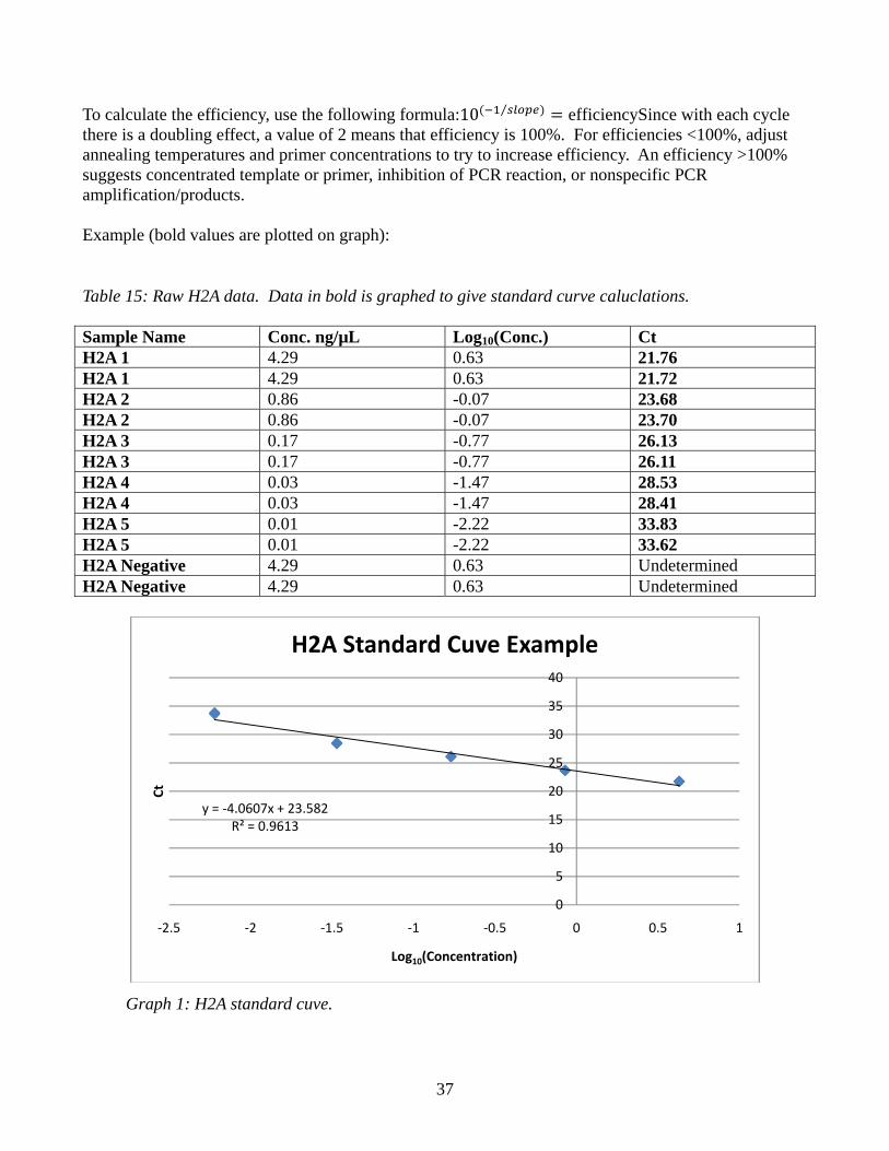
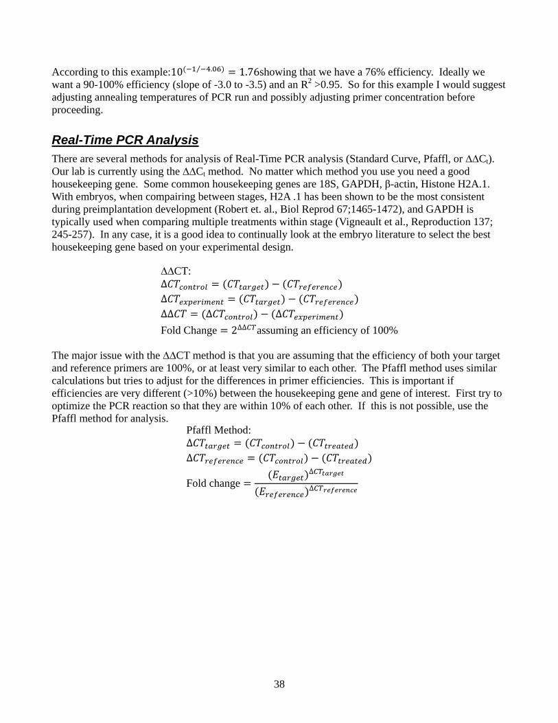
Primer Efficiency After running a standard curve (see Running a Standard Curve), export data into a spreadsheet. To calculate the efficiency, plot the standard curve with Log10(Concentration) on the x-axis and the CT value on the y-axis.
37
To calculate the efficiency, use the following formula:10 ⁄ efficiencySince with each cycle there is a doubling effect, a value of 2 means that efficiency is 100%. For efficiencies <100%, adjust annealing temperatures and primer concentrations to try to increase efficiency. An efficiency >100% suggests concentrated template or primer, inhibition of PCR reaction, or nonspecific PCR amplification/products. Example (bold values are plotted on graph):
Table 15: Raw H2A data. Data in bold is graphed to give standard curve caluclations. Sample Name Conc. ng/µL Log10(Conc.) Ct H2A 1 4.29 0.63 21.76 H2A 1 4.29 0.63 21.72 H2A 2 0.86 -0.07 23.68 H2A 2 0.86 -0.07 23.70 H2A 3 0.17 -0.77 26.13 H2A 3 0.17 -0.77 26.11 H2A 4 0.03 -1.47 28.53 H2A 4 0.03 -1.47 28.41 H2A 5 0.01 -2.22 33.83 H2A 5 0.01 -2.22 33.62 H2A Negative 4.29 0.63 Undetermined H2A Negative 4.29 0.63 Undetermined
y = ‐4.0607x + 23.582R² = 0.9613
0
5
10
15
20
25
30
35
40
‐2.5 ‐2 ‐1.5 ‐1 ‐0.5 0 0.5 1
Ct
Log10(Concentration)
H2A Standard Cuve Example
Graph 1: H2A standard cuve.
38
According to this example:10 .⁄ 1.76showing that we have a 76% efficiency. Ideally we want a 90-100% efficiency (slope of -3.0 to -3.5) and an R2 >0.95. So for this example I would suggest adjusting annealing temperatures of PCR run and possibly adjusting primer concentration before proceeding.
Real-Time PCR Analysis There are several methods for analysis of Real-Time PCR analysis (Standard Curve, Pfaffl, or ∆∆Ct). Our lab is currently using the ∆∆Ct method. No matter which method you use you need a good housekeeping gene. Some common housekeeping genes are 18S, GAPDH, β-actin, Histone H2A.1. With embryos, when compairing between stages, H2A .1 has been shown to be the most consistent during preimplantation development (Robert et. al., Biol Reprod 67;1465-1472), and GAPDH is typically used when comparing multiple treatments within stage (Vigneault et al., Reproduction 137; 245-257). In any case, it is a good idea to continually look at the embryo literature to select the best housekeeping gene based on your experimental design.
∆∆CT:∆∆∆∆ ∆ ∆Fold Change 2∆∆ assuming an efficiency of 100%
The major issue with the ∆∆CT method is that you are assuming that the efficiency of both your target and reference primers are 100%, or at least very similar to each other. The Pfaffl method uses similar calculations but tries to adjust for the differences in primer efficiencies. This is important if efficiencies are very different (>10%) between the housekeeping gene and gene of interest. First try to optimize the PCR reaction so that they are within 10% of each other. If this is not possible, use the Pfaffl method for analysis.
Pfaffl Method:∆∆
Fold change∆
∆