Polygon and transect detectors in secr 4.1Murray Efford

2019-12-07

Contents

Theory 1

Parameterisation 3

Example data: flat-tailed horned lizards 3

Data input 4

Model fitting 4

Cue data 5

Discretizing polygon data 6

Transect search 8

More on polygons 10

Solutions for non-conforming polygons . . . . . . . . . . . . . . . . . . . . . . . . . . . . . . . . . . 10

Technical notes 11

References 12

The ‘polygon’ detector type is used for data from searches of one or more areas (polygons). Transect detectorsare the linear equivalent of polygons; as the theory and implementation are very similar we mostly refer topolygon detectors and only briefly mention transects. [We do not consider here searches of linear habitatssuch as rivers]. Area and transect searches differ from other modes of detection in that each detection mayhave different coordinates, and the coordinates are continuously distributed rather than constrained to fixedpoints by the field design. The method may be used with individually identifiable cues (e.g., faeces) as wellas for direct observations of individuals.

Polygons may be independent (detector type ‘polygon’) or exclusive (detector type ‘polygonX’). Exclusivityis a particular type of dependence in which an animal may be detected at no more than one polygon on eachoccasion (i.e. polygons function more like multi-catch traps than ‘count’ detectors). Transect detectors alsomay be independent (‘transect’) or exclusive (‘transectX’).

Efford (2011) gives technical background on the fitting of polygon and transect models to spatially explicitcapture–recapture data by maximum likelihood. This document illustrates the methods using the R packagesecr. The theory is briefly sketched before moving on to an example.

Theory

This description has been modified slightly from Efford (2011), emphasising the case of independent Poisson-distributed counts for a single search area on a single occasion, and omitting the dependence of each term(Pr(n), λ(x), h(u)) on the various parameters (D, λc and σ).

1

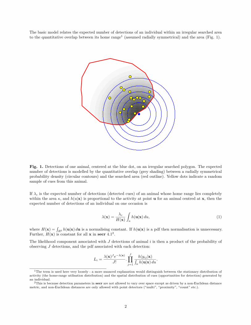
The basic model relates the expected number of detections of an individual within an irregular searched areato the quantitative overlap between its home range1 (assumed radially symmetrical) and the area (Fig. 1).

Fig. 1. Detections of one animal, centered at the blue dot, on an irregular searched polygon. The expectednumber of detections is modelled by the quantitative overlap (grey shading) between a radially symmetricalprobability density (circular contours) and the searched area (red outline). Yellow dots indicate a randomsample of cues from this animal.

If λc is the expected number of detections (detected cues) of an animal whose home range lies completelywithin the area κ, and h(u|x) is proportional to the activity at point u for an animal centred at x, then theexpected number of detections of an individual on one occasion is

λ(x) =λc

H(x)

∫κ

h(u|x) du, (1)

where H(x) =∫

R2 h(u|x) du is a normalising constant. If h(u|x) is a pdf then normalisation is unnecessary.Further, H(x) is constant for all x in secr 4.12.

The likelihood component associated with J detections of animal i is then a product of the probability ofobserving J detections, and the pdf associated with each detection:

Li =λ(x)Je−λ(x)

J !.

J∏j=1

h(yij |x)∫κ

h(u|x) du.

1The term is used here very loosely - a more nuanced explanation would distinguish between the stationary distribution ofactivity (the home-range utilisation distribution) and the spatial distribution of cues (opportunities for detection) generated byan individual.

2This is because detection parameters in secr are not allowed to vary over space except as driven by a non-Euclidean distancemetric, and non-Euclidean distances are only allowed with point detectors (“multi”, “proximity”, “count” etc.).

2

The likelihood components Li are combined across all n individuals:

L = Pr(n)

n∏i=1

Li.

Parameterisation

The detection model is fundamentally different for polygon detectors and detectors at a point (“single”,“multi”, “proximity”, “capped”, “count”):

• For point detectors, the detection function directly models the probability of detection or the expectednumber of detections. All that matters is the distance between the animal’s centre and the detector.

• For polygon detectors, these quantities (probability or expected number) depend also on the geometricalrelationships (Fig. 1) and the integration in equation 1. The detection function serves only to definethe potential detections if the search area was unbounded (blue contours in Fig. 1).

We use a parameterisation that separates two aspects of detection – the expected number of cues from anindividual (λc) and their spatial distribution given the animal’s location (h(u|x) normalised by dividing byH(x) (1). The parameters of h() are those of a typical detection function in secr (e.g., λ0, σ), except thatthe factor λ0 cancels out of the normalised expression. The expected number of cues, given an unboundedsearch area, is determined by a different parameter here labelled λc.

There are complications:

1. Rather than designate a new ‘real’ parameter lambdac, secr grabs the redundant intercept of thedetection function (lambda0) and uses that for λc. Bear this in mind when reading output from polygonor transect models.

2. If each animal can be detected at most once per detector per occasion (as with exclusive detectortypes ‘polygonX’ and ‘transectX’) then instead of λ(x) we require a probability of detection between0 and 1, say g(x). In secr 4.1 the probability of detection is derived from the cumulative hazardusing g(x) = 1 − exp(−λ(x)). The horned lizard dataset of Royle and Young (2008) has detector type‘polygonX’ and their parameter ‘p’ was equivalent to 1 − exp(−λc) (0 < p ≤ 1). For the same scenarioand parameter Efford (2011) used p∞.

3. Unrelated to (2), detection functions in secr may model either the probability of detection (HN, HR,EX etc.) or the cumulative hazard of detection (HHN, HHR, HEX etc.) (see ?detectfn for a list).Although probability and cumulative hazard are mostly interchangeable for point detectors, it’s not sosimple for polygon and transect detectors. The integration in equation 1 always uses the hazard formfor h(u|x) (secr 3.0.0 and later)3, and only hazard-based detection functions are allowed (HHN, HHR,HEX, HAN, HCG, HVP). The default function is HHN.

Example data: flat-tailed horned lizards

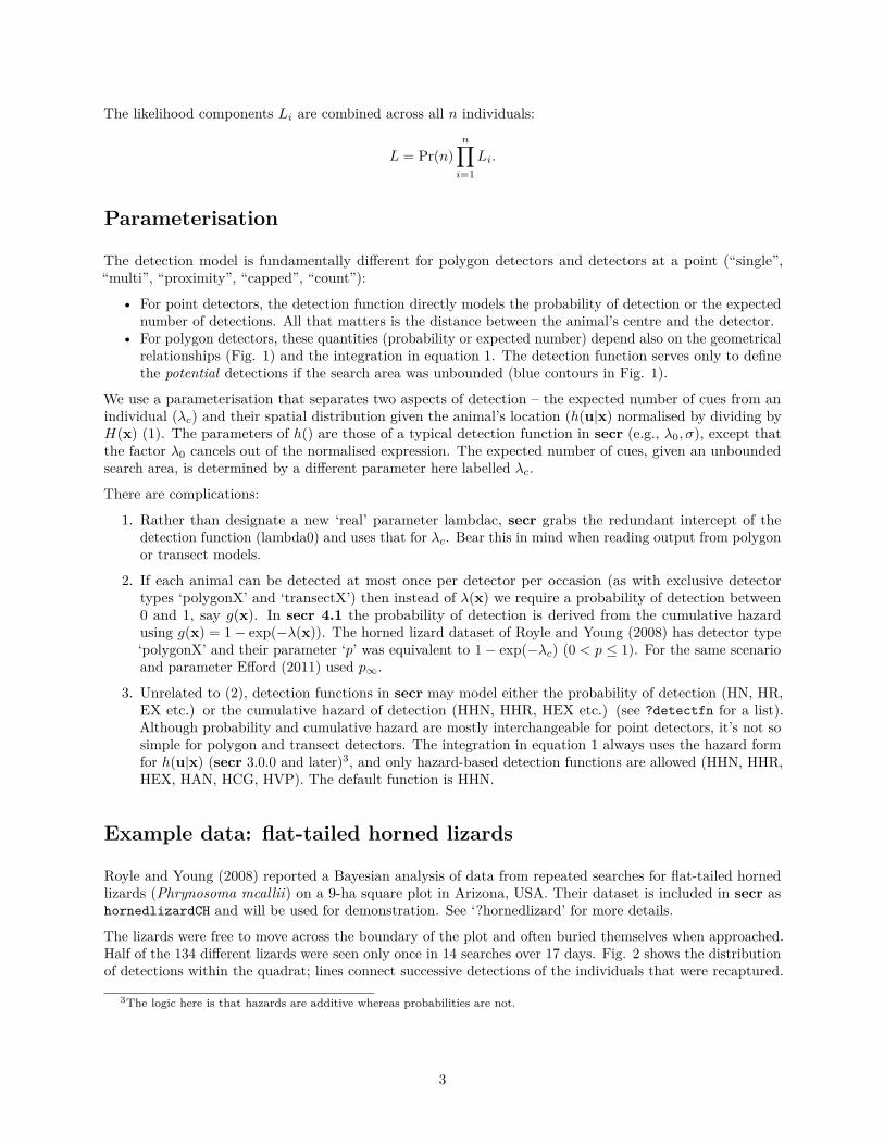
Royle and Young (2008) reported a Bayesian analysis of data from repeated searches for flat-tailed hornedlizards (Phrynosoma mcallii) on a 9-ha square plot in Arizona, USA. Their dataset is included in secr ashornedlizardCH and will be used for demonstration. See ‘?hornedlizard’ for more details.

The lizards were free to move across the boundary of the plot and often buried themselves when approached.Half of the 134 different lizards were seen only once in 14 searches over 17 days. Fig. 2 shows the distributionof detections within the quadrat; lines connect successive detections of the individuals that were recaptured.

3The logic here is that hazards are additive whereas probabilities are not.

3

par(mar=c(1,1,2,1))

plot(hornedlizardCH, tracks = TRUE, varycol = FALSE, lab1cap = TRUE, laboffset = 8,

border = 10, title ='')

1

2

3

4

56

7

8

9

10

11

12

13 14

15

16

17

18

1920

21

22

2324

25

26

272829

30

31

32

33

34

35

36

37

38

39

40

41

42 43

4445

46

47

48

49

5051

52

53

54

55

56

57

5859

6061

62

63

64

65

66

67

68

14 occasions, 134 detections, 68 animals

Fig. 2. Locations of horned lizards on a 9-ha plot in Arizona (Royle and Young 2008). Grid lines are 100 mapart.

Data input

Input of data for polygon and transect detectors is described in secr-datainput.pdf. It is little different toinput of other data for secr. The key function is read.capthist, which reads text files containing the polygonor transect coordinates4 and the capture records. Capture data should be in the ‘XY’ format of Density (onerow per record with fields in the order Session, AnimalID, Occasion, X, Y). Capture records are automaticallyassociated with polygons on the basis of X and Y (coordinates outside any polygon give an error). Transectdata are also entered as X and Y coordinates and automatically associated with transect lines.

Model fitting

The function secr.fit is used to fit polygon or transect models by maximum likelihood, exactly as for otherdetectors. Any model fitting requires a habitat mask – a representation of the region around the detectorspossibly occupied by the detected animals (aka the ‘area of integration’ or ‘state space’). It’s simplest to usea simple buffer around the detectors, specified via the ‘buffer’ argument of secr.fit5. For the horned lizard

4For constraints on the shape of polygon detectors see Polygon shape5Alternatively, one can construct a mask with make.mask and provide that in the ‘mask’ argument of secr.fit. Note that

make.mask defaults to type = 'rectangular'; see Transect search for an example in which points are dropped if they are withinthe rectangle but far from detectors (the default in secr.fit)

4

dataset it is safe to use the default buffer width (100 m) and the default detection function (circular bivariatenormal). We use trace = FALSE to suppress intermediate output that would be untidy here.

FTHL.fit <- secr.fit(hornedlizardCH, buffer = 80, trace = FALSE)

## Warning in secr.fit(hornedlizardCH, buffer = 80, trace = FALSE): using

## default starting values

predict(FTHL.fit)

## link estimate SE.estimate lcl ucl

## D log 8.0130680 1.06170100 6.1873999 10.3774218

## lambda0 log 0.1317132 0.01512831 0.1052403 0.1648453

## sigma log 18.5049025 1.19938839 16.2995006 21.0087060

The estimated density is 8.01 / ha, somewhat less than the value given by Royle and Young (2008); see Efford(2011) for an explanation, also Dorazio (2013). The parameter labelled ‘lambda0’ (i.e. λc) is equivalent to p

in Royle and Young (2008) (using p̂ ≈ 1 − exp(−λ̂c)).

FTHL.fit is an object of class secr. Many methods are available for secr objects (AIC, coef, deviance, print,etc.) – see the secr help index or Appendix 4 of secr-overview.pdf. We would use the ‘plot’ method to graphthe fitted detection function :

plot(FTHL.fit, xv = 0:70, ylab = 'p')

Cue data

By ‘cue’ in this context we mean a discrete sign identifiable to an individual animal by means such asmicrosatellite DNA. Faeces and passive hair samples may be cues. Animals may produce more than onecue per occasion. The number of cues in a specific polygon then has a discrete distribution such as Poisson,binomial or negative binomial.

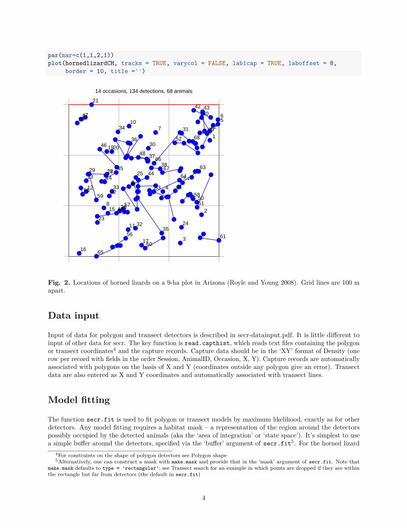
A cue dataset is not readily available, so we simulate some cue data to demonstrate the analysis. The textfile ‘temppoly.txt’ contains the boundary coordinates.

temppoly <- read.traps(file = 'temppoly.txt', detector = 'polygon')

polygonCH <- sim.capthist(temppoly, popn = list(D = 1, buffer = 200),

detectfn = 'HHN', detectpar = list(lambda0 = 5, sigma = 50),

noccasions = 1, seed = 123)

par(mar=c(1,2,3,2))

plot(polygonCH, tracks = TRUE, varycol = F, lab1cap = T, laboffset = 15,

title = paste("Simulated 'polygon' data", "D = 1, lambda0 = 5, sigma = 50"))

5

1

2

3

4

5

67

8

9

10

11

12

13

14

15

16

17

18

19

20

21

22

23

24

25

26

27

28

29

30

31

32

33

34

35

36

37

38

39

40

41

42

43

44

45

46

47

4849

50

51

52

53

54

55

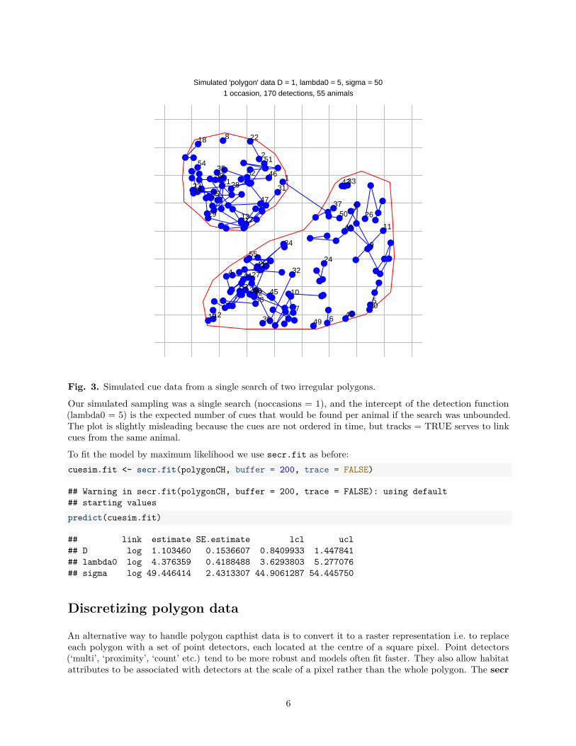
Simulated 'polygon' data D = 1, lambda0 = 5, sigma = 501 occasion, 170 detections, 55 animals

Fig. 3. Simulated cue data from a single search of two irregular polygons.

Our simulated sampling was a single search (noccasions = 1), and the intercept of the detection function(lambda0 = 5) is the expected number of cues that would be found per animal if the search was unbounded.The plot is slightly misleading because the cues are not ordered in time, but tracks = TRUE serves to linkcues from the same animal.

To fit the model by maximum likelihood we use secr.fit as before:

cuesim.fit <- secr.fit(polygonCH, buffer = 200, trace = FALSE)

## Warning in secr.fit(polygonCH, buffer = 200, trace = FALSE): using default

## starting values

predict(cuesim.fit)

## link estimate SE.estimate lcl ucl

## D log 1.103460 0.1536607 0.8409933 1.447841

## lambda0 log 4.376359 0.4188488 3.6293803 5.277076

## sigma log 49.446414 2.4313307 44.9061287 54.445750

Discretizing polygon data

An alternative way to handle polygon capthist data is to convert it to a raster representation i.e. to replaceeach polygon with a set of point detectors, each located at the centre of a square pixel. Point detectors(‘multi’, ‘proximity’, ‘count’ etc.) tend to be more robust and models often fit faster. They also allow habitatattributes to be associated with detectors at the scale of a pixel rather than the whole polygon. The secr

6

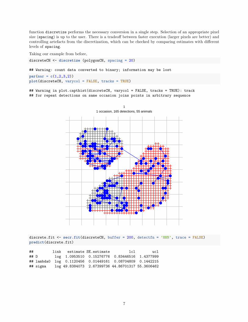
function discretize performs the necessary conversion in a single step. Selection of an appropriate pixelsize (spacing) is up to the user. There is a tradeoff between faster execution (larger pixels are better) andcontrolling artefacts from the discretization, which can be checked by comparing estimates with differentlevels of spacing.

Taking our example from before,

discreteCH <- discretize (polygonCH, spacing = 20)

## Warning: count data converted to binary; information may be lost

par(mar = c(1,2,3,2))

plot(discreteCH, varycol = FALSE, tracks = TRUE)

## Warning in plot.capthist(discreteCH, varycol = FALSE, tracks = TRUE): track

## for repeat detections on same occasion joins points in arbitrary sequence

11 occasion, 165 detections, 55 animals

discrete.fit <- secr.fit(discreteCH, buffer = 200, detectfn = 'HHN', trace = FALSE)

predict(discrete.fit)

## link estimate SE.estimate lcl ucl

## D log 1.0953510 0.15276776 0.83446516 1.4377999

## lambda0 log 0.1120456 0.01449161 0.08704809 0.1442215

## sigma log 49.8384073 2.67399736 44.86701317 55.3606462

7

Transect search

Transect data, as understood here, include the positions from which individuals are detected along a linearroute through 2-dimensional habitat. They do not include distances from the route to the location of theindividual, at least, not yet. A route may be searched multiple times, and a dataset may include multipleroutes, but neither of these is necessary. Searches of linear habitat such as river banks require a differentapproach - see the package secrlinear.

We simulate some data for an imaginary wiggly transect.

x <- seq(0, 4*pi, length = 20)

transect <- make.transect(x = x*100, y = sin(x)*300, exclusive = FALSE)

summary(transect)

## Object class traps

## Detector type transect

## Number vertices 20

## Number transects 1

## Total length 2756.105 m

## x-range 0 1256.637 m

## y-range -298.9753 298.9753 m

transectCH <- sim.capthist(transect, popn = list(D = 2, buffer = 300),

detectfn = 'HHN', detectpar = list(lambda0 = 1.0, sigma = 50),

binomN = 0, seed = 123)

By setting exclusive = FALSE we signal that there may be more than one detection per animal per occasionon this single transect (i.e. this is a ‘transect’ detector rather than ‘transectX’).

Constructing a habitat mask explicitly with make.mask (rather than relying on ‘buffer’ in secr.fit) allowsus to specify the point spacing and discard outlying points (Fig. 4).

transectmask <- make.mask(transect, type = 'trapbuffer', buffer = 300, spacing = 20)

par(mar=c(3,1,3,1))

plot(transectmask, border = 0)

plot(transect, add = TRUE, detpar = list(lwd = 2))

plot(transectCH, tracks = TRUE, add = TRUE, title = '')

8

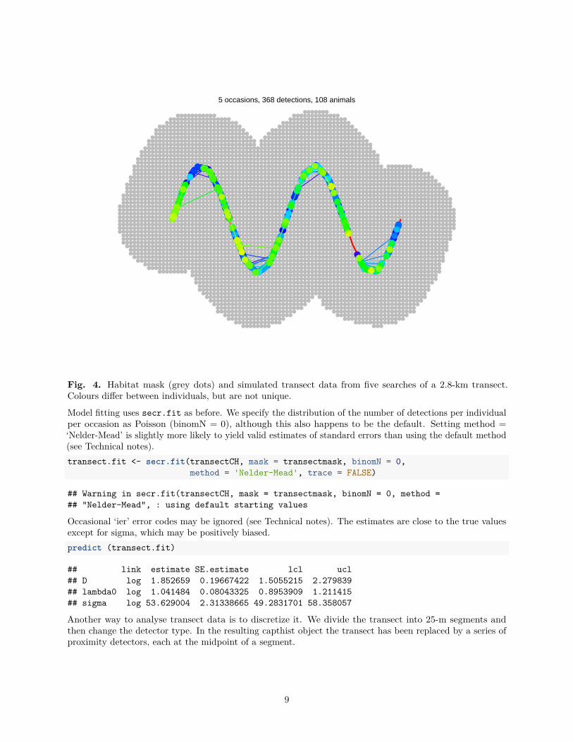
5 occasions, 368 detections, 108 animals

Fig. 4. Habitat mask (grey dots) and simulated transect data from five searches of a 2.8-km transect.Colours differ between individuals, but are not unique.

Model fitting uses secr.fit as before. We specify the distribution of the number of detections per individualper occasion as Poisson (binomN = 0), although this also happens to be the default. Setting method =‘Nelder-Mead’ is slightly more likely to yield valid estimates of standard errors than using the default method(see Technical notes).

transect.fit <- secr.fit(transectCH, mask = transectmask, binomN = 0,

method = 'Nelder-Mead', trace = FALSE)

## Warning in secr.fit(transectCH, mask = transectmask, binomN = 0, method =

## "Nelder-Mead", : using default starting values

Occasional ‘ier’ error codes may be ignored (see Technical notes). The estimates are close to the true valuesexcept for sigma, which may be positively biased.

predict (transect.fit)

## link estimate SE.estimate lcl ucl

## D log 1.852659 0.19667422 1.5055215 2.279839

## lambda0 log 1.041484 0.08043325 0.8953909 1.211415

## sigma log 53.629004 2.31338665 49.2831701 58.358057

Another way to analyse transect data is to discretize it. We divide the transect into 25-m segments andthen change the detector type. In the resulting capthist object the transect has been replaced by a series ofproximity detectors, each at the midpoint of a segment.

9

snippedCH <- snip(transectCH, by = 25)

snippedCH <- reduce(snippedCH, outputdetector = 'proximity')

The same may be achieved with newCH <- discretize(transectCH, spacing = 25). We can fit a modelusing the same mask as before. The result differs in the scaling of the lambda0 parameter, but in otherrespects is similar to that from the transect model.

snipped.fit <- secr.fit(snippedCH, mask = transectmask, detectfn = 'HHN', trace = FALSE)

predict(snipped.fit)

## link estimate SE.estimate lcl ucl

## D log 1.8421699 0.19562554 1.4968950 2.2670862

## lambda0 log 0.1931212 0.01803394 0.1608851 0.2318163

## sigma log 53.6789941 2.32112700 49.3190669 58.4243495

More on polygons

The implementation in secr allows any number of disjunct polygons or non-intersecting transects.

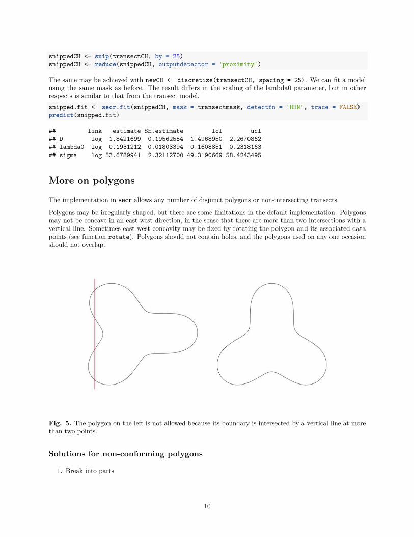
Polygons may be irregularly shaped, but there are some limitations in the default implementation. Polygonsmay not be concave in an east-west direction, in the sense that there are more than two intersections with avertical line. Sometimes east-west concavity may be fixed by rotating the polygon and its associated datapoints (see function rotate). Polygons should not contain holes, and the polygons used on any one occasionshould not overlap.

Fig. 5. The polygon on the left is not allowed because its boundary is intersected by a vertical line at morethan two points.

Solutions for non-conforming polygons

1. Break into parts

10

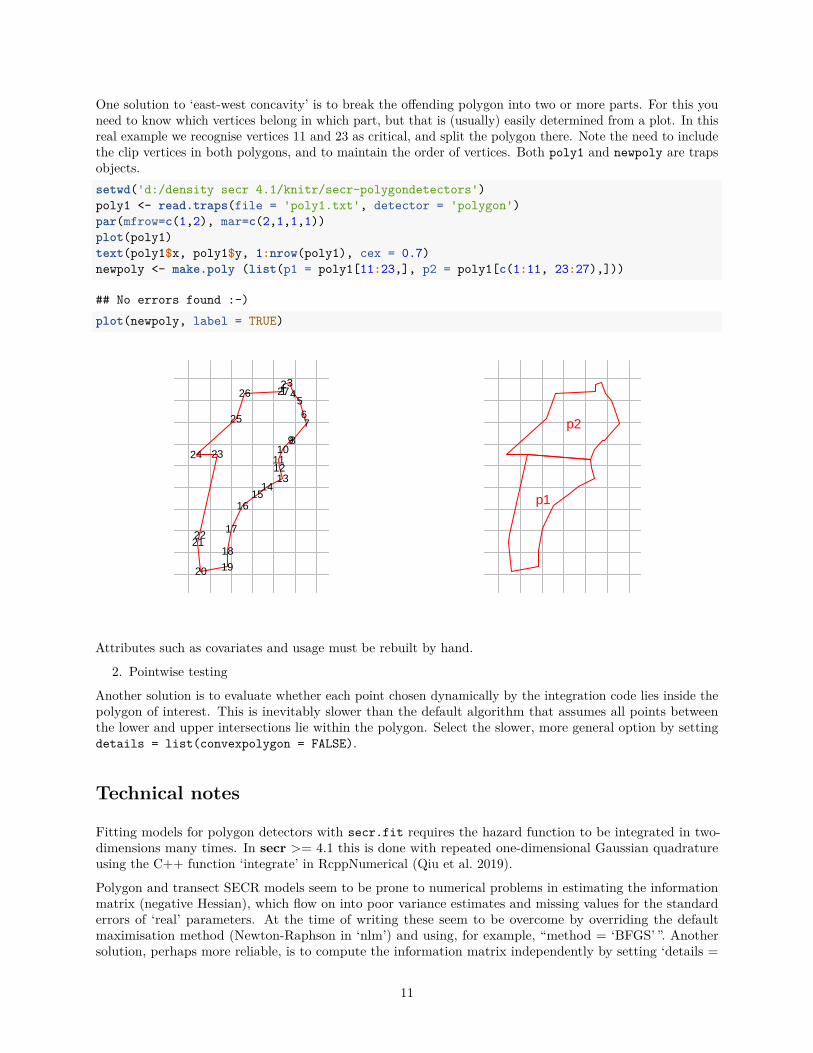
One solution to ‘east-west concavity’ is to break the offending polygon into two or more parts. For this youneed to know which vertices belong in which part, but that is (usually) easily determined from a plot. In thisreal example we recognise vertices 11 and 23 as critical, and split the polygon there. Note the need to includethe clip vertices in both polygons, and to maintain the order of vertices. Both poly1 and newpoly are trapsobjects.

setwd('d:/density secr 4.1/knitr/secr-polygondetectors')

poly1 <- read.traps(file = 'poly1.txt', detector = 'polygon')

par(mfrow=c(1,2), mar=c(2,1,1,1))

plot(poly1)

text(poly1$x, poly1$y, 1:nrow(poly1), cex = 0.7)

newpoly <- make.poly (list(p1 = poly1[11:23,], p2 = poly1[c(1:11, 23:27),]))

## No errors found :-)

plot(newpoly, label = TRUE)

123

4567

8910

111213

1415

16

17

18

1920

2122

2324

25

26 27

p1

p2

Attributes such as covariates and usage must be rebuilt by hand.

2. Pointwise testing

Another solution is to evaluate whether each point chosen dynamically by the integration code lies inside thepolygon of interest. This is inevitably slower than the default algorithm that assumes all points betweenthe lower and upper intersections lie within the polygon. Select the slower, more general option by settingdetails = list(convexpolygon = FALSE).

Technical notes

Fitting models for polygon detectors with secr.fit requires the hazard function to be integrated in two-dimensions many times. In secr >= 4.1 this is done with repeated one-dimensional Gaussian quadratureusing the C++ function ‘integrate’ in RcppNumerical (Qiu et al. 2019).

Polygon and transect SECR models seem to be prone to numerical problems in estimating the informationmatrix (negative Hessian), which flow on into poor variance estimates and missing values for the standarderrors of ‘real’ parameters. At the time of writing these seem to be overcome by overriding the defaultmaximisation method (Newton-Raphson in ‘nlm’) and using, for example, “method = ‘BFGS’ ”. Anothersolution, perhaps more reliable, is to compute the information matrix independently by setting ‘details =

11

list(hessian = ’fdhess’)’ in the call to secr.fit. Yet another approach is to apply secr.fit with “method =‘none’ ” to a previously fitted model to compute the variances.

The algorithm for finding a starting point in parameter space for the numerical maximisation is not entirelyreliable; it may be necessary to specify the ‘start’ argument of secr.fit manually, remembering that thevalues should be on the link scale (default log for D, lambda0 and sigma).

Data for polygons and transects are unlike those from detectors such as traps in several respects:

• The association between vertices in a ‘traps’ object and polygons or transects resides in an attribute‘polyID’ that is out of sight, but may be retrieved with the polyID or transectID functions. If theattribute is NULL, all vertices are assumed to belong to one polygon or transect.

• The x-y coordinates for each detection are stored in the attribute ‘detectedXY’ of a capthist object. Toretrieve these coordinates use the function xy. Detections are ordered by occasion, animal, and detector(i.e., polyID).

• subset or split applied to a polygon or transect ‘traps’ object operate at the level of whole polygonsor transects, not vertices (rows).

• usage also applies to whole polygons or transects. The option of specifying varying usage by occasionis not fully tested for these detector types.

• The interpretation of detection functions and their parameters is subtly different; the detection functionmust be integrated over 1-D or 2-D rather than yielding a probability directly (see Efford 2011).

References

Borchers, D. L. and Efford, M. G. (2008) Spatially explicit maximum likelihood methods for capture–recapturestudies. Biometrics 64, 377–385.

Dorazio, R. M. (2013) Bayes and empirical Bayes estimators of abundance and density from spatial capture–recapture data. PLoS ONE 8, e84017.

Efford, M. G. (2011) Estimation of population density by spatially explicit capture–recapture analysis ofdata from area searches. Ecology 92, 2202–2207.

Marques, T. A., Thomas, L. and Royle, J. A. (2011) A hierarchical model for spatial capture–recapture data:Comment. Ecology 92, 526–528.

Qiu, Y., Balan, S., Beall, M., Sauder, M., Okazaki, N. and Hahn, T. (2019) RcppNumerical: ‘Rcpp’Integration for Numerical Computing Libraries. R package version 0.3-3. https://CRAN.R-project.org/package=RcppNumerical

Royle, J. A. and Young, K. V. (2008) A hierarchical model for spatial capture–recapture data. Ecology 89,2281–2289.

12