Polly et al., 2016, Ecometric Modelling and Clade Dynamics

Processes of ecometric patterning: modelling functionaltraits, environments, and clade dynamics in deep time

P. DAVID POLLY1, A. MICHELLE LAWING2, JUSSI T. ERONEN3 andJAN SCHNITZLER3

1Departments of Geological Sciences, Biology and Anthropology, Indiana University, 1001 E. 10thStreet, Bloomington, IN 47405, USA2Department of Ecosystem Science and Management, Spatial Sciences Laboratory, Texas A&MUniversity, 1500 Research Parkway, Suite 223 B, 2120 TAMU, College Station, TX 77843-2120 USA3Senckenberg Biodiversity and Climate Research Centre (BiK-F), Senckenberganlage 25, D-60325Frankfurt am Main, Germany

Received 5 July 2015; revised 8 September 2015; accepted for publication 9 September 2015

Ecometric patterning is community-level sorting of functional traits along environmental gradients that ariseshistorically by geographic sorting, trait evolution, and extinction. We developed a stochastic model to explore howecometric patterns and clade dynamics emerge from microevolutionary processes. Strong selection, highprobability of extirpation, and high heritability led to strong ecometric patterning, but high rates of dispersal andweak selection do not. Phylogenetic structuring arose only when selection intensity, dispersal, and extirpation areall high. Ancestry and environmental geography produced historical effects on patterns of trait evolution andlocal diversity of species, but ecometric patterns appeared to be largely deterministic. Phylogenetic traitcorrelations and clade sorting appear to arise more easily in changing environments than static ones.Microevolutionary parameters and historical factors both affect ecometric lag time and thus balance betweenextinction, adaptation, and geographic reorganization as responses to climate change. © 2015 The LinneanSociety of London, Biological Journal of the Linnean Society, 2016, 118, 39–63.

KEYWORDS: adaptive evolution – climate change biology – ecometrics – geographic sorting – speciessorting – trait evolution.

INTRODUCTION

Earth systems – atmospheric composition, climate,ocean chemistry, sea level, and tectonics – have beenchanging since life began (Haq, 1991; Webb & Bar-tlein, 1992; Berner et al., 2003; Patzkowsky & Hol-land, 2012). Biotic communities, which are definedhere as assemblages of co-occurring species, havebeen transformed along with Earth systems as theirmembers have tracked optimal climatic or environ-mental conditions, adapted through natural selectionor environmental plasticity, diversified through spe-ciation, or succumbed to extinction (Simpson, 1944;Levins, 1968; Jablonski, 1991; Lynch & Lande, 1993;Lister, 2004; Barnosky, 2005; McPeek, 2007). Thesemodes of response are seldom exclusive, and the

balance between geographic reorganization, adaptivechange, speciation, and extinction has varied tremen-dously in Earth’s history as documented by the richstore of examples from the fossil record (Vrba, 1993;Cerling et al., 1997; Fortelius et al., 2002; Barnosky,Hadly & Bell, 2003; Lieberman, 2005; Liow & Sten-seth, 2007; Blois & Hadly, 2009; Carrasco, Barnosky& Graham, 2009; Lyons, Wagner & Dzikiewicz,2010; Barnosky, Carrasco & Graham, 2011a; Bar-nosky et al., 2011a; Hannisdal & Peters, 2011;Lawing & Polly, 2011; Willis & MacDonald, 2011).Extinction dominated the balance five times duringEarth history’s mass extinctions (Raup & Sepkoski,1982), and appears to dominate biotic change todayin the Anthropocene’s sixth extinction (Barnoskyet al., 2011b). A better understanding of what con-trols the balance between these modes of response isdesirable.

*Corresponding author. E-mail: [email protected]

39© 2015 The Linnean Society of London, Biological Journal of the Linnean Society, 2016, 118, 39–63

Biological Journal of the Linnean Society, 2016, 118, 39–63. With 5 figures.

mailto:

The mechanism by which communities respond tochanging environments is through the functionaltraits of the species that make up the communities(Ricklefs & Travis, 1980; Chapin, 1993; Poff, 1997;Wright et al., 2005; McGill et al., 2006; Webb et al.,2010; Violle et al., 2014; Jønsson, Lessard & Ricklefs,2015; Morales-Castilla et al., 2015). Species vary intheir integument cover, gas exchange surfaces, loco-motor morphology and masticatory mechanics andtherefore respond differently to factors like ambienttemperature, oxygen concentration, physical topogra-phy, predator abundance, and food quality. Func-tional traits are the tangible features of organismsthat are coupled with particular environmental fac-tors. Any particular state of the trait will performbetter in some environments than others, and thusplay a part in the overall fitness of an organism in aparticular environment. Selection and local extinc-tion will therefore tend to optimize functional traitstates along environment gradients, ceteris paribus.Environmental factors that are limiting like resourceavailability will tend to assemble communities withdiverse functional traits for acquiring resources(character displacement), whereas factors like ariditywill tend to assemble communities with similar func-tional traits for osmoregulation. Non-limiting envi-ronmental factors will therefore have a tendency toassemble communities with average trait states thatco-vary geographically with environmental gradientsacross space and time, such as with mean annualtemperature and body mass in Bergmann’s rule (e.g.,Meiri & Dayan, 2003).

We refer to the geography of functional traits asecometric patterning and we refer to the spatial cor-relation between the ecometric pattern and its asso-ciated environmental factor as ecometric correlation(Eronen et al., 2010a; Polly et al., 2011). The stron-ger the ecometric correlation, the more the traits inlocal communities co-vary with the functionalrequirements of their local environments. However,a strong ecometric correlation merely demonstratesthat the traits co-vary with the environmental factor,it does not necessarily imply that their performanceis optimal. We therefore refer to the mismatch(anomaly) between traits and their performance opti-mum as the ecometric load, analogous to the geneticloads of populations, which are the mismatchesbetween local allele frequencies and fitness optima(Haldane, 1937). A high ecometric load indicates thatmany communities have members whose traits areperforming suboptimally in their local environments,which may indicate a failure to adapt, a failure tosort, or a failure to succumb to extirpation and itimplies increased risk to current or changing condi-tions (unless the change is in a direction thatincreases trait fitness). Ecometric load is thus an

indicator of the ‘fitness’ of the overall biota. Allthings being equal, sub-optimal trait performancewill lower fitness in local populations and drive bioticchange through natural selection, dispersal, extirpa-tion, and extinction until the ecometric load is low-ered and the trait-environment relationshipequilibrates.

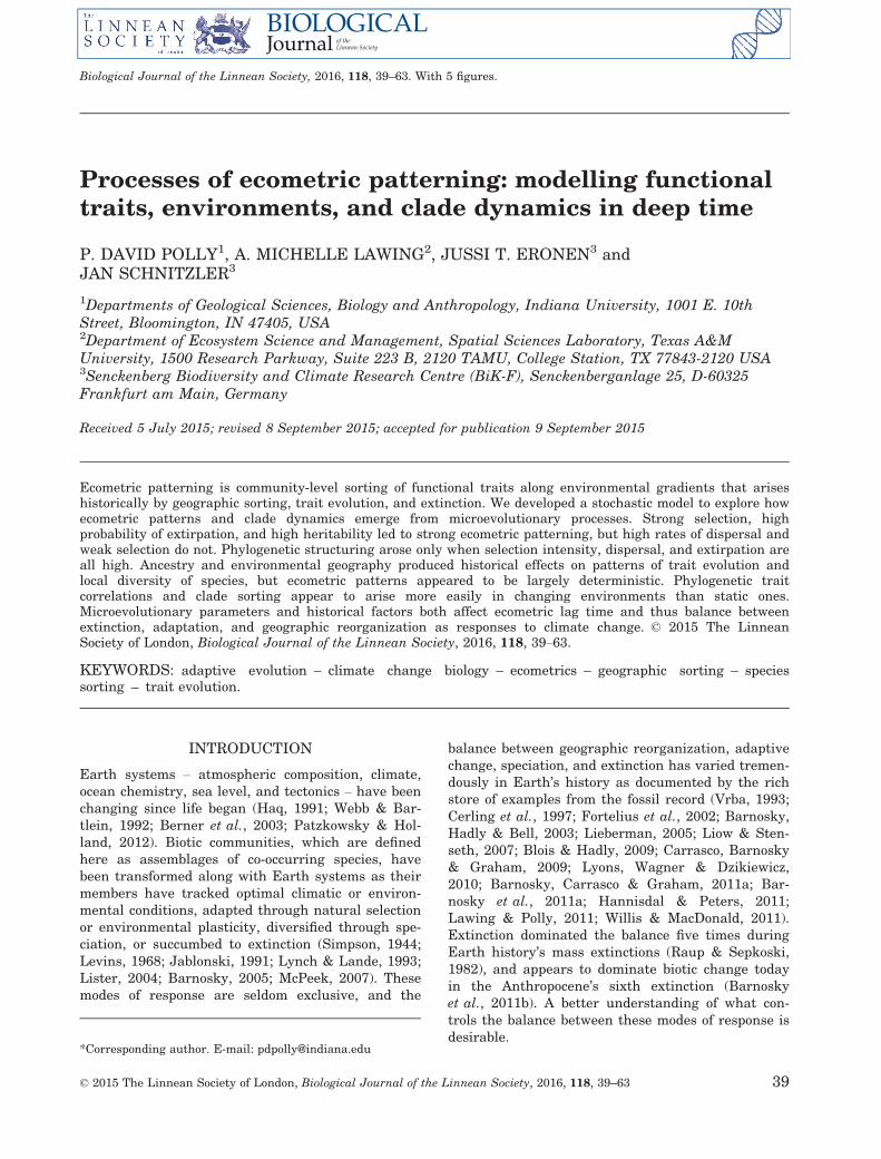
One of the clearest examples of dynamic ecometricpatterning in response to changes in Earth systemscomes from the fossil record of the geographic andtemporal spread of hypsodonty (high-crowned cheekteeth) in large herbivorous mammals, includinghorses, in response to the global spread of aridityand grasslands that resulted from the Himalayanuplift, continental reconfiguration, and changes inatmospheric and oceanic circulation (Fig. 1; Forteliuset al., 2002, 2014; Eronen et al., 2010b,c). Thischange occurred through a complex combination ofgeographic range changes, evolution, extinction, andclade sorting (MacFadden, 1985, 1992; Hulbert,1993; Vrba, 1993, 1995; Lister et al., 2005; Wolf, Ber-nor & Hussain, 2013; Fortelius et al., 2014). Commu-nity means of other functional traits such as leafshape in plants, hind limb posture in mammals, andbody proportions in snakes are also known to besorted ecometrically at continental scales (Wolfe,1993; Polly, 2010; Lawing, Head & Polly, 2012).

Because ecometric patterning emerges at the com-munity level from trait-environment interactions inmany species, it potentially involves both microevolu-tionary population-level processes and macroevolu-tionary clade dynamics (Ricklefs, 1987; Webb et al.,2002; Emerson & Gillespie, 2008; Graham & Fine,2008; Cavender-Bares et al., 2009). Microevolution-ary factors include evolvability of the traits, theeffect of mismatch between trait and environment onreproductive fitness, intensity of selection, geo-graphic isolation and gene flow, dispersal ability,and population extirpation (Lande, 1976; Hanski &Gilpin, 1991; Lynch & Lande, 1993; Holt, 1997a,b).Macroevolutionary factors that emerge frommicroevolutionary processes include convergent evo-lution of functional traits in independent lineagesthat share the same local environment, parallel evo-lution in independent lineages that experience thesame long-term environmental changes, clade-levelsorting of species into communities based on func-tional trait states shared by common ancestry, andclade turnover by extinction of one clade and radia-tion of another based on functional traits shared bycommon ancestry (Damuth, 1985; Webb et al., 2002,2010; Ackerly & Cornwell, 2007; Jablonski, 2008;Hunt & Rabosky, 2010). Indeed, it is a matter ofongoing controversy whether functional traits sharedby species in the same environment should beexpected to have evolved independently or to arise

© 2015 The Linnean Society of London, Biological Journal of the Linnean Society, 2016, 118, 39–63

40 P. D. POLLY ET AL.

by clade sorting based on functional trait states thatare shared by common ancestry (Westoby, Leishman& Lord, 1995; Little, Kembel & Wilf, 2010; Lawinget al., 2012). It is also a matter of ongoing contro-versy whether ecological processes such as commu-nity assembly are deterministic, arising predictablyfrom fundamental principles like energy budgets andnutrient availability, or whether they are historicallycontingent on the ecology of ancestors and the quirksof geography (Ricklefs, 1987, 2006). Clade-levelmacroevolutionary processes, such as modes of traitevolution (e.g., Brownian motion, stabilizing selec-tion, directional selection), phylogenetic trait correla-tion, lineage extinction and tree balance, andgeographic and temporal sorting of clades, are thusimportant to how communities respond to Earth sys-tem changes.

To better understand how ecometric patterns andclade dynamics arise from microevolutionary pro-cesses we developed a general simulation model(Gotelli et al., 2009) in which species originate, popu-lations disperse and become extirpated, functionaltraits evolve in response to environmental selectionand drift, and communities are assembled in an envi-ronmentally heterogeneous environment. Themicroevolutionary factors in our model are derived

from quantitative genetic and metapopulation the-ory: heritability, phenotypic variance, selection inten-sity, extirpation probability, dispersal probability,and population size. Our overarching goal is to deter-mine how the balance between these parameters atthe population level affects ecometric outcomes atthe community level and phylogenetic patterns oftrait evolution and community assembly at the cladelevel. Our specific aims are: (1) to explore the rangeof ecometric patterns that arise from variation inmicroevolutionary parameters; (2) to determinewhich combinations of parameters produce ecometricpatterns that match the pattern expected from thefunctional relationship between trait and environ-ment; (3) to determine the balance of parametersthat produce species sorting, clade turnover, andphylogenetic patterns of trait evolution and commu-nity assembly; (4) to determine how microevolution-ary parameters affect the balance betweengeographic range changes, extinction, and adaptiveevolution as responses to environmental change (asdiscussed below, our conclusions about responses tochange are inferences because our models were runin a heterogeneous but static environment); and (5)to assess whether ecometric patterning arises deter-ministically from the interaction between model

14 Ma (Middle Miocene)

10 Ma (Early Late Miocene)

6 Ma (Late Late Miocene)

0 31 2

Brachydont(low crowned)

Hypsodont(high crowned)

Hypsodonty metric

A

B C

Quaternary

Recent

Equus

Pliohippus

Merychippus

Mesohippus

Orohippus

Eohippus

Four Toes

Hypothetical Ancestors with Five Toes on Each Foot

Fore FootFormations in Wetern United States and Characteristic Type of Horse in Each

THE EVOLUTION OF THE HORSE.Hind Foot Teeth

Long-

One Toe

Three Toes Three Toes

Three Toes

Three Toes

Three Toes

One ToeSplints of

2nd and 4th digits

Splints of 1st and 5th digits

Side toesnot touching the ground

Side toesnot touching the ground

Side toestouching the ground

Side toestouching the ground;

splint of 5th digit

Splints of 2nd and 4th digits

Pleistocene

Pliocene

BLANCO

OGALALLA

ARICKAREE

JOHN DAY

WHITE RIVER

UINTA

PUERCO AND TORREJON

BRIDGER

WASATCH

Miocene

Oligocene

Eocene

Paleocene

Cretaceous

Jurassic

Triassic

Age of Mammals

Tertiaryor

Age of Reptiles

orAge of Man

Crowned,

Cement-

covered

Short-

Crowned,

without

Cement

and Teeth like those of Monkeys etc. like true molors

become more and more

The Premolar Teeth

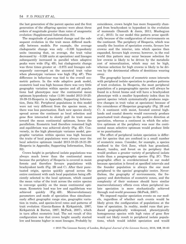
Figure 1. Hypsodonty in time and space. (A) Hypsodonty (cheek tooth crown height) increased on average in mam-

malian ungulates through the Miocene and Pliocene as global climates became more arid and grasslands spread, as

shown here in a classic diagram of horse evolution from five-toed browsers in the Eocene to single-toed grazers in the

Pliocene (from Matthew, 1926). (B) Tooth crowns range from low brachyodont forms to high hypsodont forms, quantified

from 0 to 3 (yellow to purple; colour scale used throughout figures this paper). (C) Geographic and temporal ecometric

changes in mean crown height in fossil assemblages from the Middle to Late Miocene (after Fortelius et al., 2002).


ECOMETRICS AND CLADE DYNAMICS 41

parameters and environmental gradients or whetherstochastic and historically contingent events play arole. Our modelling approach allows us to derivegeneral principles about ecometrics and cladedynamics because, not only can we control microevo-lutionary parameters, we can control the trait-envir-onment relationship and the geography ofperformance optima, all of which are challenging toestimate in real-world examples.

MODEL AND METHODS

We modelled the evolution of hypsodonty, or toothcrown height (Fig. 1). Herbivores with high-crownedteeth can tolerate a lifetime of abrasion from diets ofsilicaceous grasses or grit-covered vegetation,whereas low-crowned teeth, which are less miner-alogically expensive to produce, are adequate for lessabrasive diets (Janis & Fortelius, 1988; Damuth &Janis, 2011). Crown height thus influences whetherherbivore species are able to flourish in regions withparticular environmental conditions and, therefore,the geographic distribution of species and clades(Eronen et al., 2010b,c). Reciprocally, the regionalenvironment exerts selection on crown height andthe evolutionary response of trait evolution to envi-ronment.

Antecedents of our modelling approach include thetheoretical models of phenotypic evolution in hetero-geneous environments developed by Levins (1968)and Endler (1977); the work by Lande (1976) andArnold, Pfrender & Jones (2001) on evolution ofquantitative phenotype traits; the concepts ofmetapopulation dynamics developed by Hanski(1999), Holt (1997a), and others; and the ‘taxon-free’functional concepts of community assembly advanced

by Damuth et al. (1992), Fortelius et al. (2002),McGill et al. (2006), and others. It shares manycommon components with the geographically andphylogenetically explicit models implemented byBokma, Bokma & M€onkk€onen (2001), Rangel &Diniz-Filho (2005), Rangel, Diniz-Filho & Colwell(2007), and Roy & Goldberg (2007). See Gotelli et al.(2009) for a review of the history of macroecologicalmodelling.

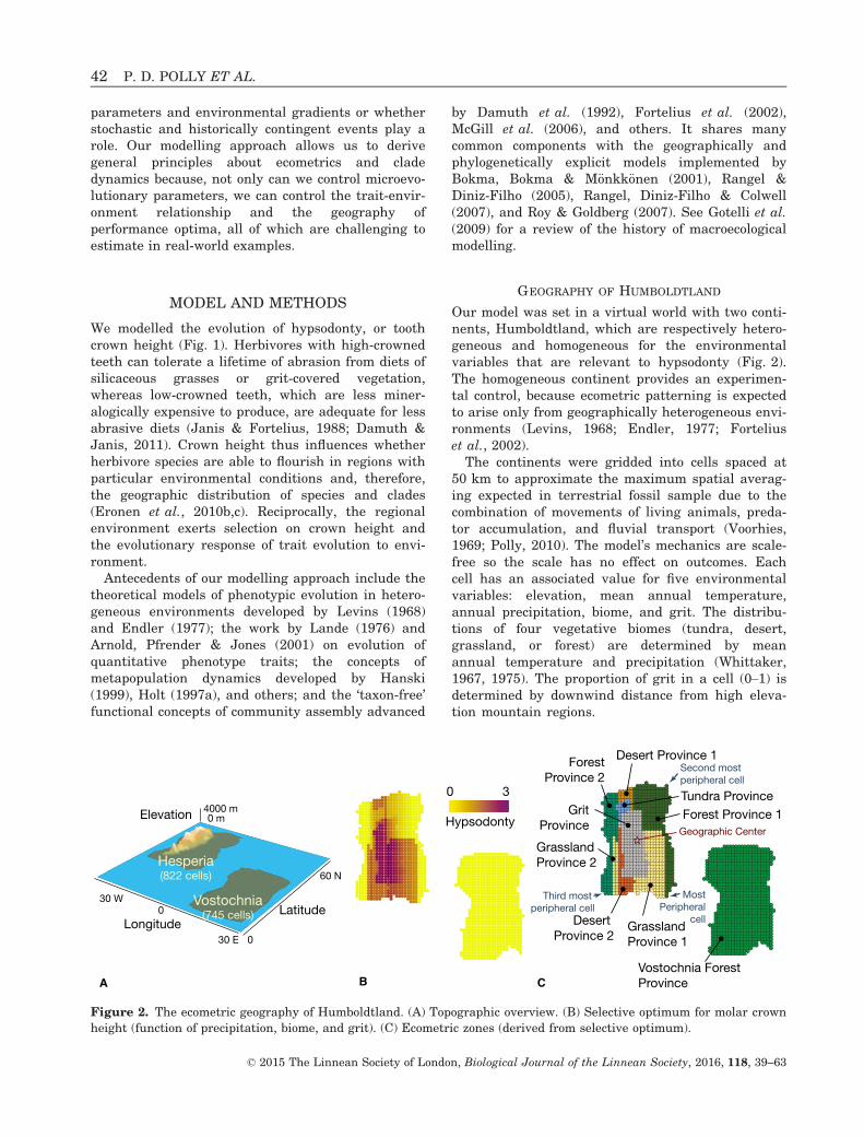
GEOGRAPHY OF HUMBOLDTLAND

Our model was set in a virtual world with two conti-nents, Humboldtland, which are respectively hetero-geneous and homogeneous for the environmentalvariables that are relevant to hypsodonty (Fig. 2).The homogeneous continent provides an experimen-tal control, because ecometric patterning is expectedto arise only from geographically heterogeneous envi-ronments (Levins, 1968; Endler, 1977; Forteliuset al., 2002).

The continents were gridded into cells spaced at50 km to approximate the maximum spatial averag-ing expected in terrestrial fossil sample due to thecombination of movements of living animals, preda-tor accumulation, and fluvial transport (Voorhies,1969; Polly, 2010). The model’s mechanics are scale-free so the scale has no effect on outcomes. Eachcell has an associated value for five environmentalvariables: elevation, mean annual temperature,annual precipitation, biome, and grit. The distribu-tions of four vegetative biomes (tundra, desert,grassland, or forest) are determined by meanannual temperature and precipitation (Whittaker,1967, 1975). The proportion of grit in a cell (0–1) isdetermined by downwind distance from high eleva-tion mountain regions.

LatitudeLongitude

Elevation

30 E

60 N

4000 m

0

0

30 W

0 m

Vostochnia(745 cells)

Hesperia(822 cells)

AVostochnia Forest Province

Forest Province 1

Desert Province 1

Tundra ProvinceGrit

Province Geographic Center

ForestProvince 2

Desert Province 2

Grassland Province 1

GrasslandProvince 2

MostPeripheral

cell

Second most peripheral cell

Third most peripheral cell

CB

30

Hypsodonty

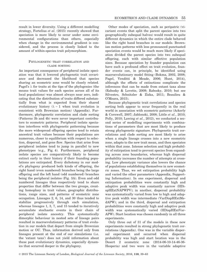
Figure 2. The ecometric geography of Humboldtland. (A) Topographic overview. (B) Selective optimum for molar crown

height (function of precipitation, biome, and grit). (C) Ecometric zones (derived from selective optimum).



The western continent, Hesperia (Latin, ‘westernland’), is situated at mid to high latitudes and is bor-dered along its western margin by a high mountainrange, and thus has steep latitudinal and altitudinaltemperature gradients and an east-west precipitationgradient. The area of Hesperia is about 2.06 millionkm2 (822 grid cells), about two-thirds the size of Aus-tralia. Areas downwind (east) of Hesperia’s highestelevations are blanketed with airborne grit. Hesperiais environmentally heterogeneous with elevationsranging from 55 to 4405 m, mean annual tempera-tures (MAT) from �9 to 19.5 °C, precipitation from10 to 199 cm per year, grit ranging from 0% to100%, and all four biomes. The eastern continent,Vostochnia (Russian, ‘eastern land’), is situated atlow latitudes, has little relief and, therefore, weaktemperature and precipitation gradients. Vos-tochnia’s area is about 1.86 million km2 (745 gridcells). Vostochnia has a comparatively uniform envi-ronment with elevations ranging from 5 to 986 m,MAT from 9.2 to 25 °C, annual precipitation from194 to 300 cm, no grit, and is completely forested.

Maps of the geographic distribution of environmen-tal variables in Humboldtland are presented in Sup-porting Information, Fig. S1 and database tables forits gridded geographic and environmental variablesare provided in Supporting Information, Table S2.

MODEL ALGORITHM

Each run of the model was 400 steps long, startingwith a single local population whose trait value wasset to its local selective optimum. The model’s param-eters affect the width of local adaptive peaks (selec-tion intensity), genetic variance, dispersal probability,and extirpation probability for the entire model run(see below and Supporting Information, Data S1).

The model simulates the functional evolution of asingle trait, molar crown height, which has valuesthat range from 0 (lowest crowned, brachyodont) to 3(highest crowned, hypsodont) (Fig. 1B). The traitvalue in each local population of each species istracked and is influenced by a combination of ances-try, local selection, gene flow, and drift. Trait valueswere averaged over all local populations to determinethe species mean trait value. Trait values were aver-aged in each grid cell over the local populations ofthe species occupying it to determine the local eco-metric mean.

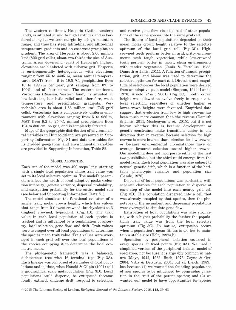
The phylogenetic framework was a balanced,dichotomous tree with 16 terminal tips (Fig. 3A).Each lineage was composed of a number of local popu-lations and is, thus, what Hanski & Gilpin (1991) calla geographical scale metapopulation (Fig. 3D). Localpopulations could disperse, be extirpated (becomelocally extinct), undergo drift, respond to selection,

and receive gene flow via dispersal of other popula-tions of the same species into the same grid cell.

The fitness of local populations depended on theirmean molar crown height relative to the selectiveoptimum of the local grid cell (Fig. 3C). High-crowned teeth perform better in arid, gritty environ-ments with tough vegetation, while low-crownedteeth perform better in moist, clean environmentswith tender vegetation (Janis & Fortelius, 1988;Damuth & Janis, 2011). A function of annual precipi-tation, grit, and biome was used to determine theselective optimum for each cell. Direction and magni-tude of selection on the local population were derivedfrom an adaptive peak model (Simpson, 1944; Lande,1976; Arnold et al., 2001) (Fig. 3C). Tooth crownheight was allowed to evolve freely in response tolocal selection, regardless of whether higher orlower-crown heights were favoured. Empirical datasuggest that evolution from low to high crowns hasbeen much more common than the reverse (Damuth& Janis, 2011; Mushegyan et al., 2015), but it is notknown whether this is because development orgenetic constraints make transitions easier in onedirection than in reverse, because selection for highcrowns is more intense than selection for low crowns,or because environmental circumstances have onaverage favoured selection toward higher crowns.Our modelling does not incorporate either of the firsttwo possibilities, but the third could emerge from themodel runs. Each local population was also subject toneutral genetic drift, which is a function of the heri-table phenotypic variance and population size(Lande, 1976).

Dispersal of local populations was stochastic, withseparate chances for each population to disperse ateach step of the model into each nearby grid cell(Fig. 3D). If a population dispersed into a cell thatwas already occupied by that species, then the phe-notypes of the incumbent and dispersing populationswere averaged to simulate gene flow.

Extirpation of local populations was also stochas-tic, with a higher probability the farther the popula-tion’s trait value was from the local selectiveoptimum (Fig. 3C). In nature, extirpation occurswhen a population’s mean fitness is too low to main-tain a stable size (Holt, 1997a,b).

Speciation by peripheral isolation occurred inevery species at fixed points (Fig. 3A). We used asimplified version of the peripheral isolates model ofspeciation, not because it is arguably common in nat-ure (Mayr, 1942, 1963; Bush, 1975; Coyne & Orr,2004; Vrba & DeGusta, 2004; but cf. Lynch, 1989),but because (1) we wanted the founding populationsof new species to be influenced by geographic varia-tion in the trait of the parent species; and (2) wewanted our model to have opportunities for species



to diverge in morphology. Peripheral isolation accom-plishes both these goals because populations alongthe periphery of the species range are likely to haveoutlying trait values because they receive less geneflow than populations in the centre and because thesmall founding populations of the peripheral isolatedescendants have a greater chance of diverging dueto selection or drift than the large, geographicallywidespread parent population (Dobzhansky, 1941;Mayr, 1963; Bush, 1975; Eldredge & Cracraft, 1980).As discussed below, the peripheral isolate mode ofspeciation had important consequences for the pat-terns that emerged from our model.

For reference, the odd numbered branches of thephylogenetic tree were always founded by a singleperipheral isolate population and the even numberedbranches, except Lineage 2, are always founded bythe remainder of the local populations of the parentspecies (Fig. 3A). Thus, half of the species in themodel demonstrate the effects of founder bottlenecksand the other half do not. This dichotomy also has

important consequences on the model’s outcomes,which are discussed below.

A complete description of the model’s algorithmsand parameters are presented in Supporting Infor-mation, Data S1. Mathematica code for a genericmodel run is given in Supporting Information, DataS3.

MODELLING EXPERIMENTS

To explore the effects of individual parameters onclade dynamics and ecometric patterns we ran fiveseries of models in which one parameter was system-atically varied and the others held constant at inter-mediate values. The full set of starting parametersfor all model runs is reported in Supporting Informa-tion, Table S1.

Experiment 1: Adaptive Peak WidthIn this experiment, four runs were performed oneach continent in which adaptive peak width (w2)

1 2

3

7

15 16 17 18 19 20 21 22 23 24 2625 27 28 29 30

8 9 10 11 12 13 14

4 5 6

Mod

el s

tep

s

0

100

200

300

400

Longitude

Latit

ude

LocalPopulations

Dispersal

Gene flow

Speciation 1

Speciation 2

Speciation 3

Speciation 4

0 31 2

Optimal Crown Heightfor local conditions

Annual Precipitation (cm)

Brachydont(low crowned)

Hypsodont(high crowned)

0 200150100500

1Grit (proportion)

0.0 1.00.50

1

Biome

0

1

Forest Tundra Desert Grassland

Local Adaptive Surface (W)(fitness of crown heightin local environment)Local Population

(Mean and variation in crown height)

Mea

n (z

)

Variance (P)

Op

tium

um (θ

i)

Peak Width (2w2)

Selectionvector (β)

Probability of local extinction (p(e))

A

DC

B

[p]

[b]

g

δ

δ

Figure 3. Components of the ecometric model. (A) Phylogenetic topology and branch identification numbers. (B) Calcu-

lation of the selective optimum (hi) for each grid cell (Fig. 2B) is based on the sum of three performance functions for

the cell’s grit proportion, annual precipitation, and vegetation. (C) For each grid cell, an adaptive peak centered at hi isused to calculate a selection vector that moves the local population toward the optimum and to determine the probability

of extirpation. Local populations occupying a same grid cell that belong to different species undergo independent selec-

tion and extirpation. (D) Each species is composed of a set of local populations that can disperse into new cells or into

cells already occupied by the species, in which case trait values are averaged to simulate gene flow.



was assigned values of 0.5, 1.0, 1.5, and 2.0 respec-tively. The width of the adaptive peak affects theintensity of selection: narrower peaks have steeperslopes and therefore more intense local selection.The width parameter is analogous to the variance ofa Gaussian (normal) distribution and is expressed insquared hypsodonty units (Fig. 3C). A value of 2.0therefore equals a ‘standard deviation’ of about 1.4units on the hypsodonty scale, which means thatalmost the entire range of crown heights are nearthe peak and have high fitness. This is very weakselection. In contrast, a value of 0.5 encompassesonly about 0.7 hypsodonty units near the fitnesspeak, which translates into very strong selectiontoward the local optimum. Note that in this paperthe term ‘adaptation’ refers to trait values that areat or near their local selective optimum because oftrait-environment selection.

Experiment 2: DispersalIn this experiment, four runs were performed oneach continent in which the probability of dispersalwas varied from 0.5 to 2.0 in 0.5 increments. Proba-bilities of 1.0 or greater meant 100% probability ofdispersal into each adjacent cell.

Experiment 3: ExtirpationIn this experiment, five runs were performed on eachcontinent in which the extirpation scaling factor wasassigned values of 0.0, 0.5, 1.0, 1.5, and 2.0 respec-tively. A factor of 0.0 means that local populationsare never extirpated, a factor of 1.0 means that theprobability of extirpation is exactly proportional tothe distance of the local population mean from theselective optimum relative to the width of the adap-tive peak.

Experiment 4: Phenotypic VarianceIn this experiment, four runs were performed oneach continent in which the phenotypic variance wasassigned values of 0.01, 0.05, 0.09, and 0.13 respec-tively. In our model, the phenotypic variance param-eter controls the amount of genetic variance, andtherefore the response of the local population toselection and the rate of genetic drift, because heri-tability (h2) is held constant at 0.5. The phenotypicvariance parameter therefore behaves similarly tothe rate parameter in macroevolutionary modelssuch as Brownian motion. A population with a smallphenotypic variance changes less in response toselection than one with a large variance, and thesame for drift.

Experiment 5: Start PointIn this experiment, the starting grid cell was ran-domly varied. Ten runs were conducted on Hesperia

to sample a reasonable range of starting environ-ments (including three out of the four biomes), andfive were conducted on Vostochnia (where there isvirtually no environmental variance to sample).

Post-hoc experimentsA second round of experiments was run to deliber-ately try to produce examples of phylogenetic correla-tion in the trait value and clade turnover, neither ofwhich emerged from the five core experiments. Inthese four experiments, three out of four key param-eters (dispersal, adaptive peak width, extirpationscaling factor, and phenotypic variance) were fixed(1.0, 0.3 2.0, 0.2 respectively) and the other one wasvaried.

ANALYTICAL METHODS

Ecometric zonesWe divided Humboldtland into discrete ecometriczones based on the continuous geographic distribu-tion of selective optima (Fig. 2). Ecometric zones arecontiguous geographic patches analogous to ecologi-cal zones (sensu Ricklefs, 2006), but are defined byenvironmental parameters that relate directly tolocal performance of a functional trait (Arnold, 1983)instead of general environmental conditions, such astemperature, precipitation, and elevation. Bound-aries between ecometric zones may be gradational orsharply defined (Whittaker, 1967; Endler, 1977;McGill et al., 2006). In our study, the combinedeffects of precipitation, vegetation cover, and ambi-ent grit define hypsodonty ecometric zones becausethese three factors affect the durability of teeth andtherefore the relative fitness of individuals in differ-ent environments (King et al., 2004, 2012). Zoneshelp distinguish effects of local adaptation from dis-persal and clade sorting from parallel adaptationbecause zones with the same selective optimum maybe separated by a sub-optimal barrier (such as thetwo forest zones in our model), and zones with differ-ent selective optima may be geographically contigu-ous (such as between forest and grit in our model).The order of spread of expanding species and cladesbetween ecometric zones helps determine whetherecometric specialization has a phylogenetic compo-nent (Ricklefs, 2006; Ackerly & Cornwell, 2007;Webb et al., 2002). Delineating ecometric zones innature may be difficult because it requires an under-standing of functional performance relative to thegeography of environmental gradients that affect itsperformance.

Ecometric loadEcometric load is a measure of how well an ecomet-ric pattern matches the pattern expected from



environmental selection. Ecometric load is analogousto genetic load, which is the difference betweenactual fitness of a population and its maximum fit-ness in a particular environment (Haldane, 1937).We calculated ecometric load as the average differ-ence between the mean trait value in local communi-ties relative to the corresponding optimal trait value:

n�1

ffiffiffiffiffiffiffiffiffiffiffiffiffiffiffiffiffiffiffiffiffiffiffiffiffiffiffiffiffiffiffiffiffiffiXn

i¼1ð�zC � hiÞ2

r; ð1Þ

where �zC is the mean trait value of the community,hi is the selective optimum for the trait in geographicgrid cell i, and n is the total number of grid cells.Ecometric load is related to ecometric correlation(R2) between an observed ecometric pattern andanother geographic variable (Polly, 2010; Lawinget al., 2012; Polly & Sarwar, 2014), but load is amore direct goodness-of-fit statistic because it doesnot scale with ecometric variance.

Ecometric equilibriumEcometric equilibrium is the ecometric load con-verged upon by a model with a particular combina-tion of parameters. Ceteris paribus, the ecometricpattern in each model reaches an equilibrium whosedistance from the selective optimum depends on theintensity of selection, gene flow, distribution of envi-ronments, and ancestry. Equilibrium is attained fas-ter with some combinations of parameters thanothers, which has implications for ecometric trackingof changing environments.

Phylogenetic signal and evolutionary ratePhylogenetic signal is a measure of the congruencebetween the distribution of trait values of lineagesand their shared evolutionary history. We usedPagel’s k (Pagel, 1999) to assess how much variationin hypsodonty could be explained by phylogeneticrelationships among the species extant at the end ofthe simulations. Note that this assumes a simpleBrownian motion model of trait evolution. Calcula-tions were performed in R (R Core Team, 2014) using

the geiger package (Harmon et al., 2008). Lineagesthat went extinct during the simulation were prunedfrom the phylogeny prior to calculating Pagel’s k.

Rates of evolutionary change could be summarizeddirectly from our models because each step changewas recorded for all branches in the tree. Becauseperipheral isolation frequently causes punctuatedbursts of change, rates of change along branches (an-agenetic) and at speciation events (cladogenetic)were calculated separately. Mean and variance werecalculated for each set of anagenetic and cladogeneticchanges respectively. The variance is equivalent to astandard phylogenetic rate parameter (e.g.,Felsen-stein, 1985; Martins & Hansen, 1997; Revell, Har-mon & Collar, 2008), and the mean is an indicator ofdirectionality (e.g., Butler & King, 2004; Polly, 2004;Hunt, 2006). The rate statistics are reported in Sup-porting Information, Table S1.

Geographic summary statisticsGeographic variance is the intraspecific variance intrait values among local populations; mean geo-graphic variance is its average across all species atthe end of the model run. Range size is calculated asthe number of grid cells a species occupies in propor-tion to the total number of grid cells in the continent;mean range size is averaged across all species at theend of the model run. Species richness is the totalnumber of species occupying a grid cell at the end ofthe model run, and mean richness is the averageacross all grid cells.

Phylogenetic community patternsPhylogenetic structure of species composition in localcommunities can be an important clue to the cladedynamics of community assembly (Webb et al., 2002;Ricklefs, 2006; Emerson & Gillespie, 2008; Cavender-Bares et al., 2009) and by extension to the historicalprocesses underlying ecometric patterns. Phylogenieswere mapped onto ecometric zones as one method forassessing phylogenetic structuring (e.g., third columnof Fig. 4). We measured community relatedness foreach grid cell as the evolutionary branch lengths

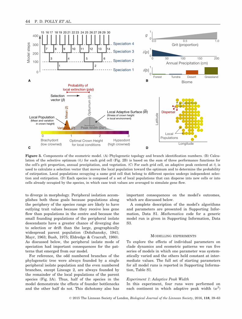
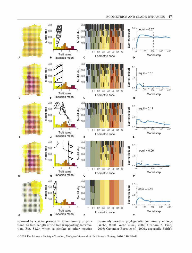
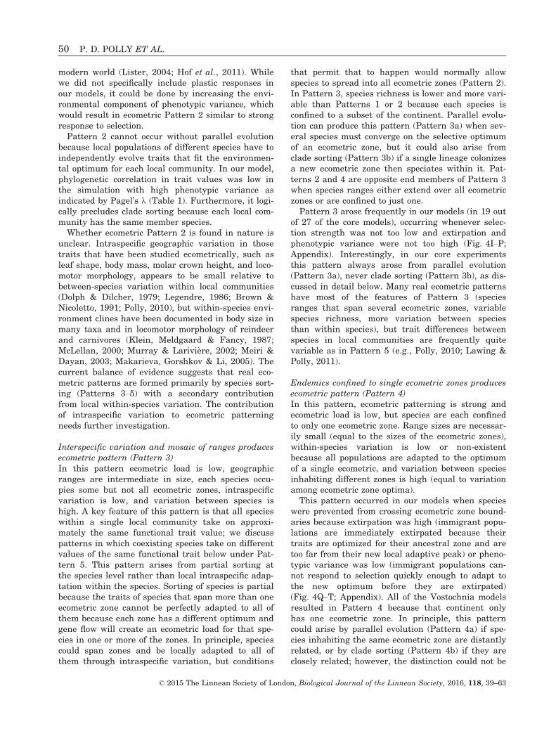
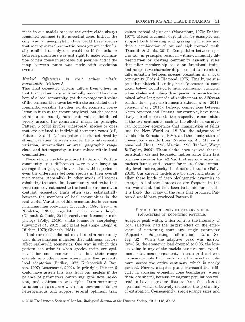
Figure 4. Examples of five ecometric patterns arising from the model experiments. (A–D) Pattern 1. Adaptive peak

experiment, w2=2.0 (2013-10-25-18-39-15-Hesperia). (E–H) Pattern 2. Phenotypic variance experiment, r2 = 0.13 (2013-

10-25-18-21-39-Hesperia). (I–L) Pattern 3a. Start location experiment, start zone = grit (2013-10-25-22-02-06-Hesperia).

(M–P) Pattern 3b. Variable peak, high dispersal and extirpation experiment, w2 = 1.0, disp = 1.0, extirp = 2.0 (2014-06-

10-10-47-02-Hesperia). (Q–T) Pattern 4. Extirpation experiment, extirp = 1.0 (2013-10-25-19-24-20-Hesperia). First col-

umn shows the ecometric pattern at step 400 of each model; the second column shows changes in the trait mean of each

species; the third column shows phylogenetic pattern of geographic spread through ecometric zones (layout of branches

follows Fig. 3A); and the fourth column shows change in the ecometric load (average difference per grid cell between

ecometric pattern and the selective optimum shown in Fig. 2B) as blue line, equilibrium load as horizontal grey line,

and the time at which equilibrium is reached as broken vertical line.



spanned by species present in a community propor-tional to total length of the tree (Supporting Informa-tion, Fig. S1.2), which is similar to other metrics

commonly used in phylogenetic community ecology(Webb, 2000; Webb et al., 2002; Graham & Fine,2008; Cavender-Bares et al., 2009), especially Faith’s

equil = 0.57

equil = 0.16

equil = 0.10

equil = 0.17

equil = 0.06

0 1 2 3

100

200

300

400

Trait value(species mean)

Ecometric zone

Mod

el s

tep

100

200

300

400

Mod

el s

tep

T F1 F2 G1 G2 D2 D1 G0.0

0.5

1.0

Eco

met

ric lo

ad

0 100 200 300 400

Model step

0 1 2 3

100

200

300

400


Ecometric zone

Mod

el s

tep

100

200

300

400

Mod

el s

tep

T F1 F2 G1 G2 D2 D1 G0.0

0.5

1.0

Eco

met

ric lo

ad

0 100 200 300 400

Model step

0 1 2 3

100

200

300

400


Ecometric zone

Mod

el s

tep

100

200

300

400

Mod

el s

tep

T F1 F2 G1 G2 D2 D1 G0.0

0.5

1.0

Eco

met

ric lo

ad0 100 200 300 400

Model step

0 1 2 3

100

200

300

400


Ecometric zone

Mod

el s

tep

100

200

300

400

Mod

el s

tep

T F1 F2 G1 G2 D2 D1 G0.0

0.5

1.0

Eco

met

ric lo

ad

0 100 200 300

Model step

0 1 2 3

100

200

300

400


Ecometric zone

Mod

el s

tep

100

200

300

400

Mod

el s

tep

T F1 F2 G1 G2 D2 D1 G0.0

0.5

1.0

Eco

met

ric lo

ad

0 100 200 300 400

Model step

A B C D

E F G H

I J K L

M N O P

Q R S T



original phylogenetic diversity metric (Faith, 1992).To correct for chance sampling, the proportion isreported as the P-value that is higher or lower thana randomly selected group of species of the samenumber. Note that P-values were calculated relativeto the complete tree (Fig. 3A) regardless of branchesthat became extinct during the model. A communitycan have higher or lower relatedness than expectedby chance because of either geographic exclusion orextinction, which are quickly distinguished byinspection of extinction patterns. These results arepresented in map form in Supporting Information,Data S2.

GUIDE TO MODEL OUTPUT

A summary of key statistics from the core modelruns on Hesperia is reported in Appendix and a fullsummary of statistics is reported in SupportingInformation, Table S1. Graphic output of ecometricpatterns, species ranges, species richness patterns,phylogenetic change in trait means, and geographicpatterns of community relatedness are presented inSupporting Information, Data S2. Graphs showingthe change in ecometric load and the final ecomet-ric equilibrium of each model are shown in Sup-porting Information, Fig. S2. Phylogenetic diagramsshowing the history of ecometric zone occupationare shown in Supporting Information, Fig. S3. Ani-mations showing the development of ecometric pat-tern through the course of each model run arepackaged in Supporting Information, Tables S3 andS4. It is recommended that readers refer to at leasta few of the output graphics (Data S2) and anima-tions (Tables S3 and S4) as an aid to understand-ing discussion of our results.

RESULTS AND DISCUSSION

ECOMETRIC PATTERNS, THEIR CAUSES, AND THEIR

INTERPRETATION

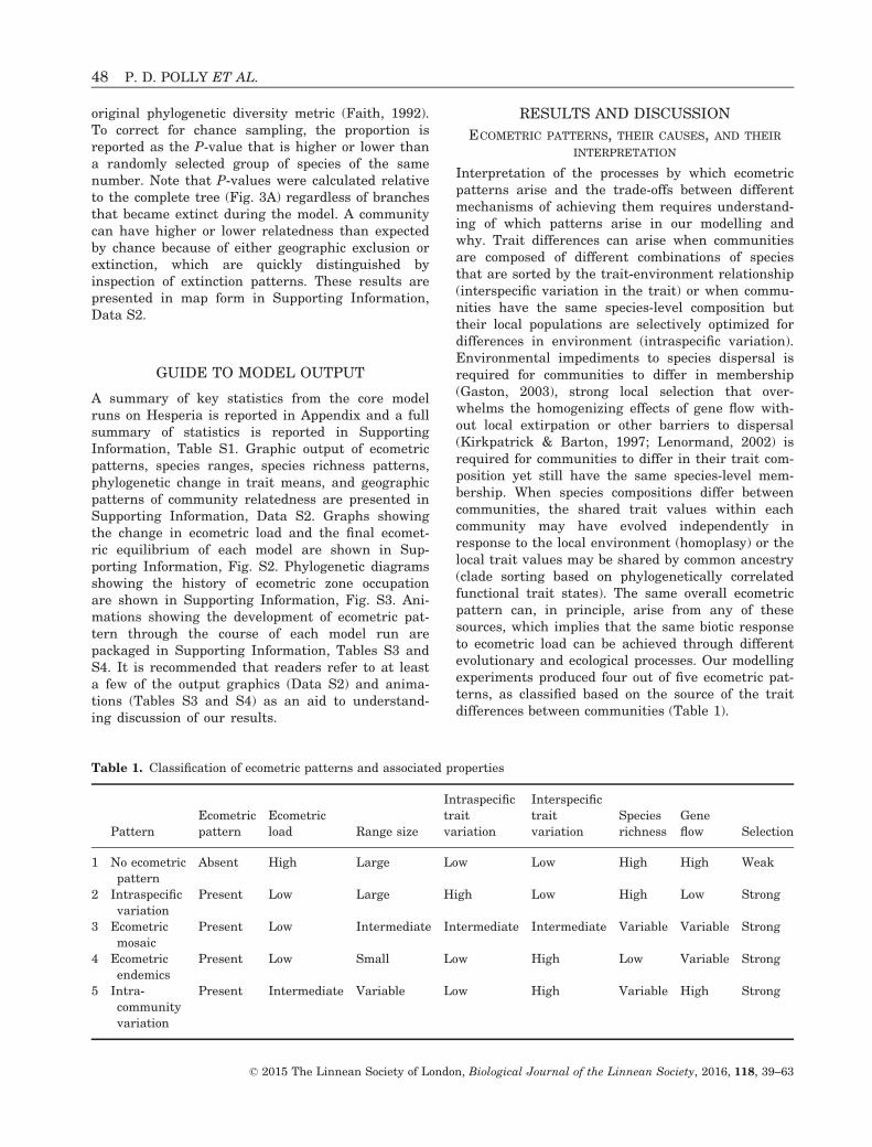
Interpretation of the processes by which ecometricpatterns arise and the trade-offs between differentmechanisms of achieving them requires understand-ing of which patterns arise in our modelling andwhy. Trait differences can arise when communitiesare composed of different combinations of speciesthat are sorted by the trait-environment relationship(interspecific variation in the trait) or when commu-nities have the same species-level composition buttheir local populations are selectively optimized fordifferences in environment (intraspecific variation).Environmental impediments to species dispersal isrequired for communities to differ in membership(Gaston, 2003), strong local selection that over-whelms the homogenizing effects of gene flow with-out local extirpation or other barriers to dispersal(Kirkpatrick & Barton, 1997; Lenormand, 2002) isrequired for communities to differ in their trait com-position yet still have the same species-level mem-bership. When species compositions differ betweencommunities, the shared trait values within eachcommunity may have evolved independently inresponse to the local environment (homoplasy) or thelocal trait values may be shared by common ancestry(clade sorting based on phylogenetically correlatedfunctional trait states). The same overall ecometricpattern can, in principle, arise from any of thesesources, which implies that the same biotic responseto ecometric load can be achieved through differentevolutionary and ecological processes. Our modellingexperiments produced four out of five ecometric pat-terns, as classified based on the source of the traitdifferences between communities (Table 1).

Table 1. Classification of ecometric patterns and associated properties

Pattern

Ecometric

pattern

Ecometric

load Range size

Intraspecific

trait

variation

Interspecific

trait

variation

Species

richness

Gene

flow Selection

1 No ecometric

pattern

Absent High Large Low Low High High Weak

2 Intraspecific

variation

Present Low Large High Low High Low Strong

3 Ecometric

mosaic

Present Low Intermediate Intermediate Intermediate Variable Variable Strong

4 Ecometric

endemics

Present Low Small Low High Low Variable Strong

5 Intra-

community

variation

Present Intermediate Variable Low High Variable High Strong



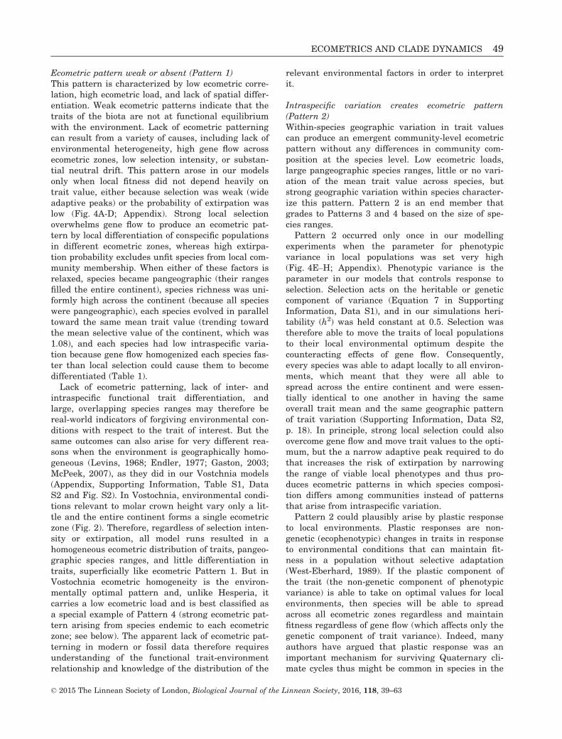
Ecometric pattern weak or absent (Pattern 1)This pattern is characterized by low ecometric corre-lation, high ecometric load, and lack of spatial differ-entiation. Weak ecometric patterns indicate that thetraits of the biota are not at functional equilibriumwith the environment. Lack of ecometric patterningcan result from a variety of causes, including lack ofenvironmental heterogeneity, high gene flow acrossecometric zones, low selection intensity, or substan-tial neutral drift. This pattern arose in our modelsonly when local fitness did not depend heavily ontrait value, either because selection was weak (wideadaptive peaks) or the probability of extirpation waslow (Fig. 4A-D; Appendix). Strong local selectionoverwhelms gene flow to produce an ecometric pat-tern by local differentiation of conspecific populationsin different ecometric zones, whereas high extirpa-tion probability excludes unfit species from local com-munity membership. When either of these factors isrelaxed, species became pangeographic (their rangesfilled the entire continent), species richness was uni-formly high across the continent (because all specieswere pangeographic), each species evolved in paralleltoward the same mean trait value (trending towardthe mean selective value of the continent, which was1.08), and each species had low intraspecific varia-tion because gene flow homogenized each species fas-ter than local selection could cause them to becomedifferentiated (Table 1).

Lack of ecometric patterning, lack of inter- andintraspecific functional trait differentiation, andlarge, overlapping species ranges may therefore bereal-world indicators of forgiving environmental con-ditions with respect to the trait of interest. But thesame outcomes can also arise for very different rea-sons when the environment is geographically homo-geneous (Levins, 1968; Endler, 1977; Gaston, 2003;McPeek, 2007), as they did in our Vostchnia models(Appendix, Supporting Information, Table S1, DataS2 and Fig. S2). In Vostochnia, environmental condi-tions relevant to molar crown height vary only a lit-tle and the entire continent forms a single ecometriczone (Fig. 2). Therefore, regardless of selection inten-sity or extirpation, all model runs resulted in ahomogeneous ecometric distribution of traits, pangeo-graphic species ranges, and little differentiation intraits, superficially like ecometric Pattern 1. But inVostochnia ecometric homogeneity is the environ-mentally optimal pattern and, unlike Hesperia, itcarries a low ecometric load and is best classified asa special example of Pattern 4 (strong ecometric pat-tern arising from species endemic to each ecometriczone; see below). The apparent lack of ecometric pat-terning in modern or fossil data therefore requiresunderstanding of the functional trait-environmentrelationship and knowledge of the distribution of the

relevant environmental factors in order to interpretit.

Intraspecific variation creates ecometric pattern(Pattern 2)Within-species geographic variation in trait valuescan produce an emergent community-level ecometricpattern without any differences in community com-position at the species level. Low ecometric loads,large pangeographic species ranges, little or no vari-ation of the mean trait value across species, butstrong geographic variation within species character-ize this pattern. Pattern 2 is an end member thatgrades to Patterns 3 and 4 based on the size of spe-cies ranges.

Pattern 2 occurred only once in our modellingexperiments when the parameter for phenotypicvariance in local populations was set very high(Fig. 4E–H; Appendix). Phenotypic variance is theparameter in our models that controls response toselection. Selection acts on the heritable or geneticcomponent of variance (Equation 7 in SupportingInformation, Data S1), and in our simulations heri-tability (h2) was held constant at 0.5. Selection wastherefore able to move the traits of local populationsto their local environmental optimum despite thecounteracting effects of gene flow. Consequently,every species was able to adapt locally to all environ-ments, which meant that they were all able tospread across the entire continent and were essen-tially identical to one another in having the sameoverall trait mean and the same geographic patternof trait variation (Supporting Information, Data S2,p. 18). In principle, strong local selection could alsoovercome gene flow and move trait values to the opti-mum, but the a narrow adaptive peak required to dothat increases the risk of extirpation by narrowingthe range of viable local phenotypes and thus pro-duces ecometric patterns in which species composi-tion differs among communities instead of patternsthat arise from intraspecific variation.

Pattern 2 could plausibly arise by plastic responseto local environments. Plastic responses are non-genetic (ecophenotypic) changes in traits in responseto environmental conditions that can maintain fit-ness in a population without selective adaptation(West-Eberhard, 1989). If the plastic component ofthe trait (the non-genetic component of phenotypicvariance) is able to take on optimal values for localenvironments, then species will be able to spreadacross all ecometric zones regardless and maintainfitness regardless of gene flow (which affects only thegenetic component of trait variance). Indeed, manyauthors have argued that plastic response was animportant mechanism for surviving Quaternary cli-mate cycles thus might be common in species in the



modern world (Lister, 2004; Hof et al., 2011). Whilewe did not specifically include plastic responses inour models, it could be done by increasing the envi-ronmental component of phenotypic variance, whichwould result in ecometric Pattern 2 similar to strongresponse to selection.

Pattern 2 cannot occur without parallel evolutionbecause local populations of different species have toindependently evolve traits that fit the environmen-tal optimum for each local community. In our model,phylogenetic correlation in trait values was low inthe simulation with high phenotypic variance asindicated by Pagel’s k (Table 1). Furthermore, it logi-cally precludes clade sorting because each local com-munity has the same member species.

Whether ecometric Pattern 2 is found in nature isunclear. Intraspecific geographic variation in thosetraits that have been studied ecometrically, such asleaf shape, body mass, molar crown height, and loco-motor morphology, appears to be small relative tobetween-species variation within local communities(Dolph & Dilcher, 1979; Legendre, 1986; Brown &Nicoletto, 1991; Polly, 2010), but within-species envi-ronment clines have been documented in body size inmany taxa and in locomotor morphology of reindeerand carnivores (Klein, Meldgaard & Fancy, 1987;McLellan, 2000; Murray & Larivi�ere, 2002; Meiri &Dayan, 2003; Makarieva, Gorshkov & Li, 2005). Thecurrent balance of evidence suggests that real eco-metric patterns are formed primarily by species sort-ing (Patterns 3–5) with a secondary contributionfrom local within-species variation. The contributionof intraspecific variation to ecometric patterningneeds further investigation.

Interspecific variation and mosaic of ranges producesecometric pattern (Pattern 3)In this pattern ecometric load is low, geographicranges are intermediate in size, each species occu-pies some but not all ecometric zones, intraspecificvariation is low, and variation between species ishigh. A key feature of this pattern is that all specieswithin a single local community take on approxi-mately the same functional trait value; we discusspatterns in which coexisting species take on differentvalues of the same functional trait below under Pat-tern 5. This pattern arises from partial sorting atthe species level rather than local intraspecific adap-tation within the species. Sorting of species is partialbecause the traits of species that span more than oneecometric zone cannot be perfectly adapted to all ofthem because each zone has a different optimum andgene flow will create an ecometric load for that spe-cies in one or more of the zones. In principle, speciescould span zones and be locally adapted to all ofthem through intraspecific variation, but conditions

that permit that to happen would normally allowspecies to spread into all ecometric zones (Pattern 2).In Pattern 3, species richness is lower and more vari-able than Patterns 1 or 2 because each species isconfined to a subset of the continent. Parallel evolu-tion can produce this pattern (Pattern 3a) when sev-eral species must converge on the selective optimumof an ecometric zone, but it could also arise fromclade sorting (Pattern 3b) if a single lineage colonizesa new ecometric zone then speciates within it. Pat-terns 2 and 4 are opposite end members of Pattern 3when species ranges either extend over all ecometriczones or are confined to just one.

Pattern 3 arose frequently in our models (in 19 outof 27 of the core models), occurring whenever selec-tion strength was not too low and extirpation andphenotypic variance were not too high (Fig. 4I–P;Appendix). Interestingly, in our core experimentsthis pattern always arose from parallel evolution(Pattern 3a), never clade sorting (Pattern 3b), as dis-cussed in detail below. Many real ecometric patternshave most of the features of Pattern 3 (speciesranges that span several ecometric zones, variablespecies richness, more variation between speciesthan within species), but trait differences betweenspecies in local communities are frequently quitevariable as in Pattern 5 (e.g., Polly, 2010; Lawing &Polly, 2011).

Endemics confined to single ecometric zones producesecometric pattern (Pattern 4)In this pattern, ecometric patterning is strong andecometric load is low, but species are each confinedto only one ecometric zone. Range sizes are necessar-ily small (equal to the sizes of the ecometric zones),within-species variation is low or non-existentbecause all populations are adapted to the optimumof a single ecometric, and variation between speciesinhabiting different zones is high (equal to variationamong ecometric zone optima).

This pattern occurred in our models when specieswere prevented from crossing ecometric zone bound-aries because extirpation was high (immigrant popu-lations are immediately extirpated because theirtraits are optimized for their ancestral zone and aretoo far from their new local adaptive peak) or pheno-typic variance was low (immigrant populations can-not respond to selection quickly enough to adapt tothe new optimum before they are extirpated)(Fig. 4Q–T; Appendix). All of the Vostochnia modelsresulted in Pattern 4 because that continent onlyhas one ecometric zone. In principle, this patterncould arise by parallel evolution (Pattern 4a) if spe-cies inhabiting the same ecometric zone are distantlyrelated, or by clade sorting (Pattern 4b) if they areclosely related; however, the distinction could not be



made in our models because the entire clade alwaysremained confined to its ancestral zone. Indeed, theonly way a monophyletic clade could have speciesthat occupy several ecometric zones yet are individu-ally confined to only one would be if the balancebetween parameters was just right to make coloniza-tion of new zones improbable but possible and if thejump between zones was made with speciationevents.

Marked differences in trait values withincommunities (Pattern 5)This final ecometric pattern differs from others inthat trait values vary substantially among the mem-bers of a local community, yet the average trait valueof the communities covaries with the associated envi-ronmental variable. In other words, ecometric corre-lation is high at the community level, but the specieswithin a community have trait values distributedwidely around the community mean. In principle,Pattern 5 could involve widespread species or onesthat are confined to individual ecometric zones (c.f.,Patterns 3 and 4). This pattern is characterized bystrong variation between species, little intraspecificvariation, intermediate or small geographic rangesizes, and heterogeneity in trait values within localcommunities.

None of our models produced Pattern 5. Within-community trait differences were never larger onaverage than geographic variation within species oreven the differences between species in their overalltrait means (Appendix). In other words, all speciescohabiting the same local community had traits thatwere similarly optimized to the local environment. Incontrast, ecometric traits often vary substantiallybetween the members of local communities in thereal world. Variation within communities is commonin mammalian body mass (Legendre, 1986; Brown &Nicoletto, 1991), ungulate molar crown height(Damuth & Janis, 2011), carnivoran locomotor mor-phology (Polly, 2010), snake locomotor morphology(Lawing et al., 2012), and plant leaf shape (Dolph &Dilcher, 1979; Givnesh, 1984).

That our models did not result in intra-communitytrait differentiation indicates that additional factorsaffect real-world ecometrics. One way in which thispattern can arise is when species traits are opti-mized for one ecometric zone, but their rangeextends into other zones where gene flow preventslocal adaptation (Endler, 1977; Kirkpatrick & Bar-ton, 1997; Lenormand, 2002). In principle, Pattern 5could have arisen this way from our models if thebalance of parameters controlling gene flow, selec-tion, and extirpation was right. Intra-communityvariation can also arise when local environments areheterogeneous and support several optimum trait

values instead of just one (MacArthur, 1972; Endler,1977). Mixed savannah vegetation, for example, cansupport both browsing and grazing herbivores andthus a combination of low and high-crowned teeth(Damuth & Janis, 2011). Competition between spe-cies can, in principle, result in within-community dif-ferentiation by creating community assembly rulesthat filter membership based on functional traits,and competitive character displacement can reinforcedifferentiation between species coexisting in a localcommunity (Cody & Diamond, 1975). Finally, we sus-pect that historical contingencies (discussed in moredetail below) would add to intra-community variationwhen clades with deep divergences in ancestry aremixed after long periods of confinement to differentcontinents or past environments (Linder et al., 2014;Jønsson et al., 2015). Periodic connections betweenNorth America and Eurasia, for example, have itera-tively mixed clades into the respective communitiesof the two continents, such as the effects on carnivo-ran locomotor ecometrics that immigration of felidsinto the New World ca. 18 Ma, the migration ofcanids into Eurasia ca. 9 Ma, and the immigration ofcrown-group ursids from Eurasia ca. 4.5 Ma musthave had (Hunt, 1998; Martin, 1998; Tedford, Wang& Taylor, 2009). These clades have evolved charac-teristically distinct locomotor indices since their lastcommon ancestor (ca. 42 Ma) that are now mixed inmodern faunas and account for most of the commu-nity-level heterogeneity in functional traits (Polly,2010). Our current models are too short and static toallow these kinds of deep phylogenetic dynamics toemerge. All of these processes are frequent in thereal world and, had they been built into our models,it is likely that many of the runs that produced Pat-tern 3 would have produced Pattern 5.

EFFECTS OF MICROEVOLUTIONARY MODEL

PARAMETERS ON ECOMETRIC PATTERNS

Adaptive peak width, which controls the intensity oflocal selection, had the largest effect on the emer-gence of patterning than any single parameter(Appendix; Supporting Information, Data S2,Fig. S2). When the adaptive peak was narrow(w2=0.5), the ecometric load dropped to 0.05, the low-est value in any of the models our five core experi-ments (i.e., mean hypsodonty in each grid cell wason average only 0.05 units from the selective opti-mum across the entire continent, which is nearlyperfect). Narrow adaptive peaks increased the diffi-culty in crossing ecometric zone boundaries (wherethese are sharp), because immigrant populations willtend to have a greater distance from the selectiveoptimum, which effectively increases the probabilityof extirpation. Consequently, species-range sizes and



the number of ecometric zones occupied by each spe-cies was on average lower when peak width was nar-rower. Note, however, that narrow peaks were not aseffective at limiting dispersal as raising the extirpa-tion probability. Narrow adaptive peaks encouragedinterspecific differences among species if they occu-pied different ecometric zones, but encouraged simi-larity among species if they were endemic to thesame zone or were pangeographic across all zones.As peak width increased (w2 ≥ 1.5), ecometric loadincreased, species ranges tended toward being pan-geographic, and ecometric patterning disappearedbecause local selection weakened enough that geneflow swamped any differentiation – all populations ofall species converged on the continent’s averageselective optimum (1.01 for Hesperia).

Dispersal probability, which is the probability of alocal population expanding into a nearby cell,affected the time required for a new species tospread and the rate of gene flow (Appendix; Support-ing Information, Data S2). The effects of dispersalwere most obvious in the post-hoc experimentswhere dispersal probability was varied from 0.2 to1.0 (VarDispHExtMedAPW; see below), whichdemonstrated that range size and species richnessboth increase as dispersal becomes more probable.The lowest dispersal probabilities were associatedwith low intraspecific geographic variance, which isarguably counterintuitive because one would expectthat low gene flow would allow local selection tocause differentiation across the geographic range;however, low dispersal probability also decreased thelikelihood that populations would cross ecometriczone boundaries and thus confined them to a morehomogeneous environment, which produced less geo-graphic variation despite lack of gene flow (Kirk-patrick & Barton, 1997) (see for example ExperimentVarDispHExtMedAPW, Model 2014-06-10-08-20-20-Hesperia).

Extirpation probability had largely the oppositeeffect of adaptive peak width: when the extirpationscaling factor was low, species tended to be pangeo-graphic with little ecometric differentiation (Pattern1), but as it increased traits became more locally dif-ferentiated and species tended to be more geographi-cally restricted (Pattern 3), ultimately being confinedto a single ecometric zone (Pattern 4) (Appendix;Supporting Information, Table S1). Extirpation andpeak width have subtle but important differencesthough, because weak extirpation allows unfit popu-lations to survive without being selected toward thelocal adaptive optimum, for example when gene flowcounteracts local selection, even though selectionmay be intense, whereas wide adaptive peaks pro-duce less intense selection because a wider range ofphenotypes are fit.

Phenotypic variance within a local populationincreases its response to selection in our modelsbecause it has the effect of increasing genetic vari-ance because we held heritability (h2) constant. Apopulation with higher genetic variance thusresponded more to local selection in our models thanone with low variance. Low phenotypic variance pre-vented populations from crossing ecometric zoneboundaries because they could not adapt quicklyenough to avoid extirpation, resulting in species withranges confined to a single ecometric zone (pattern4), but with a relatively high ecometric load (similarto pattern 1) (Appendix; Supporting Information,Table S1, Data S2). When phenotypic variance waslow species were frequently excluded from some eco-metric zones, in large part because the inability torespond to selection caused drift and gene flow tobecome more important in carrying populations awayfrom the local selective optimum and making themmore vulnerable to extirpation (Supporting Informa-tion, Fig. S3) (see Kirkpatrick & Barton, 1997;Lenormand, 2002). As phenotypic variance increases,average range size and intraspecific variationincrease and ecometric load and between-species dif-ferentiation decrease (grading through Pattern 3 to2).

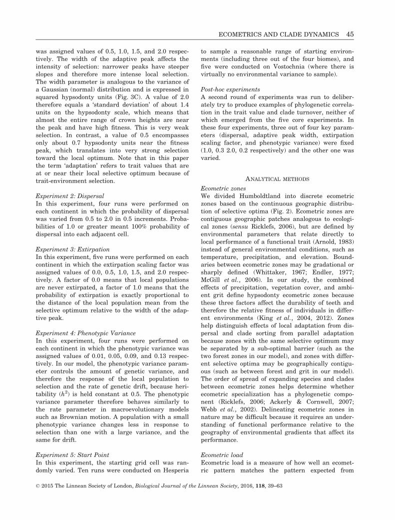
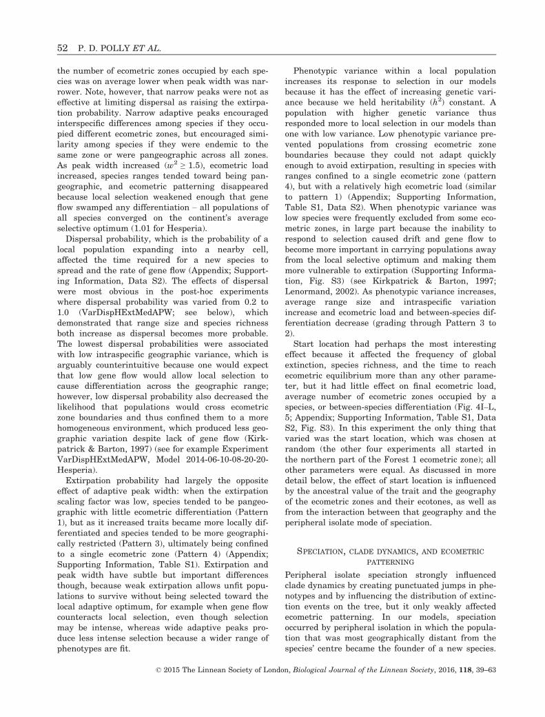
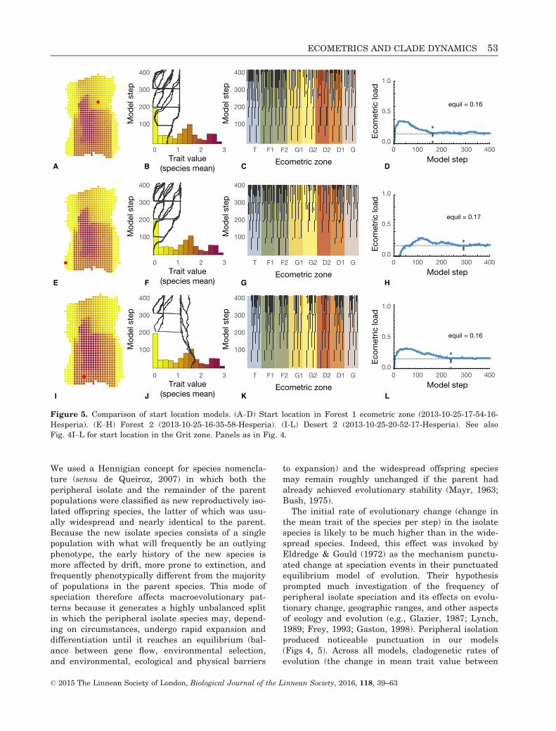
Start location had perhaps the most interestingeffect because it affected the frequency of globalextinction, species richness, and the time to reachecometric equilibrium more than any other parame-ter, but it had little effect on final ecometric load,average number of ecometric zones occupied by aspecies, or between-species differentiation (Fig. 4I–L,5; Appendix; Supporting Information, Table S1, DataS2, Fig. S3). In this experiment the only thing thatvaried was the start location, which was chosen atrandom (the other four experiments all started inthe northern part of the Forest 1 ecometric zone); allother parameters were equal. As discussed in moredetail below, the effect of start location is influencedby the ancestral value of the trait and the geographyof the ecometric zones and their ecotones, as well asfrom the interaction between that geography and theperipheral isolate mode of speciation.

SPECIATION, CLADE DYNAMICS, AND ECOMETRIC

PATTERNING

Peripheral isolate speciation strongly influencedclade dynamics by creating punctuated jumps in phe-notypes and by influencing the distribution of extinc-tion events on the tree, but it only weakly affectedecometric patterning. In our models, speciationoccurred by peripheral isolation in which the popula-tion that was most geographically distant from thespecies’ centre became the founder of a new species.



We used a Hennigian concept for species nomencla-ture (sensu de Queiroz, 2007) in which both theperipheral isolate and the remainder of the parentpopulations were classified as new reproductively iso-lated offspring species, the latter of which was usu-ally widespread and nearly identical to the parent.Because the new isolate species consists of a singlepopulation with what will frequently be an outlyingphenotype, the early history of the new species ismore affected by drift, more prone to extinction, andfrequently phenotypically different from the majorityof populations in the parent species. This mode ofspeciation therefore affects macroevolutionary pat-terns because it generates a highly unbalanced splitin which the peripheral isolate species may, depend-ing on circumstances, undergo rapid expansion anddifferentiation until it reaches an equilibrium (bal-ance between gene flow, environmental selection,and environmental, ecological and physical barriers

to expansion) and the widespread offspring speciesmay remain roughly unchanged if the parent hadalready achieved evolutionary stability (Mayr, 1963;Bush, 1975).

The initial rate of evolutionary change (change inthe mean trait of the species per step) in the isolatespecies is likely to be much higher than in the wide-spread species. Indeed, this effect was invoked byEldredge & Gould (1972) as the mechanism punctu-ated change at speciation events in their punctuatedequilibrium model of evolution. Their hypothesisprompted much investigation of the frequency ofperipheral isolate speciation and its effects on evolu-tionary change, geographic ranges, and other aspectsof ecology and evolution (e.g., Glazier, 1987; Lynch,1989; Frey, 1993; Gaston, 1998). Peripheral isolationproduced noticeable punctuation in our models(Figs 4, 5). Across all models, cladogenetic rates ofevolution (the change in mean trait value between

equil = 0.17

equil = 0.16

equil = 0.16

0 1 2 3

100

200

300

400


Ecometric zone

Mod

el s

tep

100

200

300

400

Mod

el s

tep

T F1 F2 G1 G2 D2 D1 G0.0

0.5

1.0

Eco

met

ric lo

ad

0 100 200 300 400

Model step

0 1 2 3

100

200

300

400


Ecometric zone

Mod

el s

tep

100

200

300

400

Mod

el s

tep

T F1 F2 G1 G2 D2 D1 G0.0

0.5

1.0

Eco

met

ric lo

ad

0 100 200 300 400

Model step

0 1 2 3

100

200

300

400


Ecometric zone

Mod

el s

tep

100

200

300

400

Mod

el s

tep

T F1 F2 G1 G2 D2 D1 G0.0

0.5

1.0

Eco

met

ric lo

ad0 100 200 300 400

Model step

A B C D

E F G H

I J K L

Figure 5. Comparison of start location models. (A–D) Start location in Forest 1 ecometric zone (2013-10-25-17-54-16-

Hesperia). (E–H) Forest 2 (2013-10-25-16-35-58-Hesperia). (I-L) Desert 2 (2013-10-25-20-52-17-Hesperia). See also

Fig. 4I–L for start location in the Grit zone. Panels as in Fig. 4.



the last generation of the parent species and the firstgeneration of the offspring species) were about threeorders of magnitude greater than rates of anageneticevolution (Supplemental Information S3).

The magnitude of punctuated change and the sub-sequent evolution in the trait mean differed mark-edly between models. For example, the averagecladogenetic change was only �0.326 hypsodontyunits (meaning that, on average, the trait valuedecreased by �0.326 units at speciation) and lineagessubsequently increased in parallel when adaptivepeaks were wide (Fig. 4B), but cladogenetic changewas three times greater at �0.975 and lineages sub-sequently converged on the ancestral trait valuewhen phenotypic variance was high (Fig. 4F). Thisdifference in behaviour was tied to the overall eco-metric pattern. In the wide adaptive peak model,ecometric load was high because there was very littlegeographic variation within species and all popula-tions had phenotypes near the continental meanoptimum hypsodonty value (1.08) (model 2013-10-25-18-39-15-Hesperia in Appendix; Supporting Informa-tion, Data S2). Peripheral populations in this modelwere not very different from the species mean, sothere was less punctuation. Each new species slowlyspread across the continent as local selection andgene flow interacted to slowly pull its trait meantoward the mean continental optimum, hence theparallelism. Ecometric load therefore remained highand equilibrium was achieved slowly (Fig. 4D). Con-versely, in the high phenotypic variance model, geo-graphic variation within species was high becausethe traits of local populations were always near thelocal selective optimum (model 2013-10-25-18-21-39-Hesperia in Appendix; Supporting Information, DataS2).

Crown height in peripheral isolate populations wasalways much lower than the continental meanbecause the periphery of Hesperia is covered in moistforests and therefore favours populations withbrachyodont teeth (Fig. 2B and C). After their punc-tuated origin, species quickly spread across theentire continent with each local population being effi-ciently selected to the local optimum, which causedthe mean value of the trait across the entire speciesto converge quickly on the mean continental opti-mum. Ecometric load was low and equilibrium wasachieved quickly (Fig. 4H). Microevolutionaryparameters and mode of speciation thus simultane-ously affect geographic range size, geographic varia-tion in traits, and species-level rates and patterns oftrait evolution (Garc�ıa-Ramos & Kirkpatrick, 1997;Kirkpatrick & Barton, 1997; McPeek, 2007), whichin turn affect ecometric load. The net result of thisconfiguration was that crown height usually startedlow and became higher in most lineages. Probably by

coincidence, crown height has more frequently chan-ged from brachyodont to hypsodont in the evolutionof mammals (Damuth & Janis, 2011; Mushegyanet al., 2015). In our model this pattern arose specifi-cally because of the configuration of environments onthe continent. The periphery of Hesperia, which wasusually the location of speciation events, favours lowcrowns and the interior, into which species thenexpanded, favours high crowns; however, in the realworld this pattern may occur because selection forlow crowns is likely to be driven by the metaboliccost of mineralization, which may not be high,whereas selection for high crowns is likely to be dri-ven by the detrimental effects of dentitions wearingaway.

The geographic layout of ecometric zones interactswith peripheral isolate speciation to produce patternsof trait evolution. In Hesperia, the most peripheralpopulation of a pangeographic species will always befound in a forest biome and will have a brachyodontphenotype with a smaller hypsodonty index than itsparent species (which systematically produces nega-tive changes in trait value at speciation) because ofthe coincidence of Hesperian geography (Fig. 2B andC). A continent with moist, forested central high-lands and coastal deserts would conversely producepunctuated trait changes in the positive direction atspeciation, whereas a continent in which the selec-tive optimum at the periphery was near the conti-nental mean selective optimum would produce littleor no punctuation.

The effect of peripheral isolate speciation is differ-ent for species that are confined to a small numberof ecometric zones. Consider, for example, a speciesconfined to the Grit Zone, which has grassland,desert, tundra, and forest on its periphery thatwould produce a greater variety of peripheral isolatetraits than a pangeographic species (Fig. 2C). Thisgeographic effect is overdetermined in our modelbecause speciation is forced at specified intervals andthe founder population is always the one mostperipheral to the species’ geographic centre. Never-theless, the geography of environments, the fre-quency and distribution of ecometric zones, and thecomplexity of their ecotones should have similarmacroevolutionary effects even when peripheral iso-late speciation is more stochastically achievedthrough real-world processes (McPeek, 2007).

We imposed regular speciation events on our mod-els, regardless of whether such events would belikely given the configuration of populations at thetime of speciation. In reality, model runs that pro-duced geographically widespread, phenotypicallyhomogeneous species with high rates of gene flowwould not likely result in peripheral isolate popula-tions, which would inhibit speciation and would



result in lower diversity. Using a different modellingstrategy, Fortelius et al. (2015) recently showed thatspeciation is more likely to occur under some envi-ronmental configurations than others, especiallywhen change in the environmental gradient is con-sidered, and the process is closely linked to theamount of within-species trait polymorphism.

PHYLOGENETIC TRAIT CORRELATION AND

CLADE SORTING

An important consequence of peripheral isolate speci-ation was that it lowered phylogenetic trait covari-ance and decreased the likelihood that speciessharing an ecometric zone would be closely related.Pagel’s k for traits at the tips of the phylogenies (themeans trait values for each species across all of itslocal populations) was almost always near zero, indi-cating that the distribution of traits differed substan-tially from what is expected from their sharedevolutionary history (k = 1 when trait evolution isconsistent with Brownian motion) (Appendix). Fur-thermore, phylogenetic correlation and clade sorting(Patterns 3b and 4b) were never important contribu-tors to ecometric patterns. Peripheral isolate specia-tion interferes with phylogenetic patterning becausethe more widespread offspring species tend to retainancestral trait values because their populations arenumerous, closer to equilibrium with respect to selec-tion, dispersal, and gene flow. Species that arise fromperipheral isolates tend to jump in parallel to newphenotypes (e.g., Fig. 4). Furthermore, peripheralisolate species are comparatively likely to becomeextinct early in their history if their founding popu-lations are extirpated. Every dichotomy in our mod-el’s phylogeny produced both kinds of offspring, theright hand (even numbered) branches being the largeoffspring and the left hand (odd numbered) branchesbeing the peripheral isolates (Fig. 3A). Even and oddnumbered lineages thus respectively tend to shareproperties that differ between the two groups, creat-ing homoplasy in trait values, geographic distribu-tions, range sizes, and patterns of ecometric zoneoccupation. Lineages 2, 6, 14, and 30 thus tended tostabilize progressively through each simulation,whereas lineages 1, 3, 7, and 15 tended to iterativelyaccumulate stochastic events in their chain ofperipheral isolate ancestry. This systematicallydimorphic behaviour in nested sets of lineage pairsresulted in macroevolutionary patterns of trait evolu-tion in our models that depart from simple Brownianmotion or OU. Thus, information derived only fromlineages present at the end of our simulations (i.e.the ‘extant taxa’) does not yield information aboutthese past evolutionary dynamics, especially dynam-ics that occurred deeper in the phylogeny.

Other modes of speciation, such as peripatric (vi-cariant events that split the parent species into twogeographically subequal halves) would result in quitedifferent dynamics in which the entire clade behavedlike the right hand branches in our models. Brown-ian motion patterns with less pronounced punctuatedspeciation events would be much more likely if speci-ation divided the parent species into two subequaloffspring, each with similar effective populationsizes. Because speciation by founder population canhave such a profound effect on trait evolution, foun-der events can, in principle, be identified usingmacroevolutionary model fitting (Bokma, 2002, 2008;Pagel, Venditti & Meade, 2006; Hunt, 2014),although the effects of extinctions complicate theinferences that can be made from extant taxa alone(Rabosky & Lovette, 2009; Rabosky, 2010; but seeSilvestro, Schnitzler & Zizka, 2011; Beaulieu &O’Meara, 2015).

Because phylogenetic trait correlations and speciessorting both appear to occur frequently in the realworld in association with ecometric patterns (Ackerly& Cornwell, 2007; Jablonski, 2008; Little et al., 2010;Polly, 2010; Lawing et al., 2012), we conducted a sec-ond series of modelling experiments with combina-tions of parameters that are most likely to producestrong phylogenetic signature. Phylogenetic trait cor-relations and clade sorting are most likely to arisewhen a single lineage crosses into a new ecometriczone, adapts to the new trait mean, and then speciateswithin that zone. Intense selection and high probabil-ity of extirpation tend to prevent species from expand-ing across zone boundaries, whereas high dispersalprobability increases the number of attempts at cross-ing. Low phenotypic variance also lowers the chanceof populations establishing themselves in new ecomet-ric zones. Thus, we set extirpation probability highand varied the other parameters (Appendix, Support-ing Information). In one experiment, dispersal andextirpation probabilities were constantly high andadaptive peak width was constantly narrow (HDi-spHExtNAPWPV); in another, dispersal probabilitywas systematically varied from low to high and adap-tive peak width was intermediate (VarDispHExtMe-dAPW); and in the third, dispersal and extirpationprobabilities were constantly high and adaptive peakwidth was systematically varied (HDispHExtVar-APW). Start location was chosen randomly in all threeexperiments.

Only three out of 31 of the models in these newexperiments resulted in strong phylogenetic trait cor-relations (Appendix). One was in the variable disper-sal experiment and occurred when dispersalprobability was high and start location was in theDesert 2 ecometric zone (2014-06-10-14-46-36-Hesperia) and two were in the variable adaptive



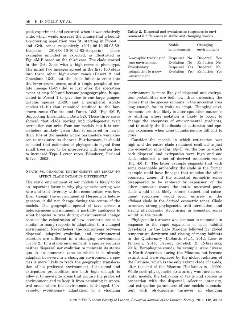
peak experiment and occurred when it was relativelywide, which would increase the chance that a bound-ary-crossing population was fit, starting in Forest 1and Grit zones respectively (2014-06-10-05-05-59-Hesperia, 2014-06-10-10-47-02-Hesperia). Theseexamples unfolded as expected, as illustrated inFig. 4M-P based on the third case. The clade startedin the Grit Zone with a high-crowned phenotype.The initial two lineages spread in the first 100 stepsinto three other high-crown zones (Desert 2 andGrassland 1&2), but the clade failed to cross intothe lower-crown zones until a single peripheral iso-late lineage (L-09) did so just after the speciationevent at step 200 and became pangeographic. It spe-ciated in Forest 1 to give rise to one large pangeo-graphic species (L-20) and a peripheral isolatespecies (L-19) that remained confined to the low-crown zones (Tundra and Forest 1&2) (Fig. 4M–P,Supporting Information, Data S2). These three casesshowed that clade sorting and phylogenetic traitcorrelation can arise from our models, but it is nev-ertheless unlikely given that it occurred in fewerthan 10% of the models where parameters were cho-sen to maximize its chances. Furthermore, it shouldbe noted that estimates of phylogenetic signal fromsmall trees need to be interpreted with caution dueto increased Type I error rates (Blomberg, Garland& Ives, 2003).

STATIC VS. CHANGING ENVIRONMENTS ARE LIKELY TO

AFFECT CLADE DYNAMICS DIFFERENTLY

The static environment of our models is likely to bean important factor in why phylogenetic sorting wasrare and trait diversity within communities was low.Even though the environment of Hesperia is hetero-geneous, it did not change during the course of themodels. The geographic spread of taxa across aheterogeneous environment is partially analogous towhat happens to taxa during environmental changebecause the colonization of new ecometric zones issimilar in many respects to adaptation to a changedenvironment. Nevertheless, the connections betweendispersal, adaptive evolution, and environmentalselection are different in a changing environment(Table 2). In a stable environment, a species requiresneither dispersal nor evolution to maintain its statusquo in an ecometric zone to which it is alreadyadapted; however, in a changing environment a spe-cies is more likely to track the geographic transloca-tion of its preferred environment if dispersal andextirpation probabilities are both high enough toallow it to move into areas that acquire the preferredenvironment and to keep it from persisting in ances-tral areas where the environment is changed. Con-versely, evolutionary adaptation to a changing

environment is more likely if dispersal and extirpa-tion probabilities are both low, thus increasing thechance that the species remains in the ancestral arealong enough for its traits to adapt. Changing envi-ronments are thus likely to alter speciation outcomesby shifting where isolation is likely to occur, tochange the steepness of environmental gradients,and to modify the likelihoods of extinction and spe-cies expansion when zone boundaries are difficult tocross.

Consider the models in which extirpation washigh and the entire clade remained confined to justone ecometric zone (Fig. 4Q–T) vs. the one in whichboth dispersal and extirpation were high and oneclade colonized a set of derived ecometric zones(Fig. 4M–P). The latter example suggests that withsome reasonable probability the clade in the formerexample could have lineages that colonize the otherecometric zones. If the ancestral ecometric zonesdisappeared to be replaced by expansion of theother ecometric zones, the entire ancestral para-clade would most likely become extinct and subse-quent speciation would occur entirely in theoffshoot clade in the derived ecometric zones. Cladeturnover, strong phylogenetic trait correlation, andstrong phylogenetic structuring in ecometric zoneswould be the result.

Phylogenetic turnover was common in mammals inresponse to the rapid expansion of open habitatgrasslands in the Late Miocene followed by globaltemperature downturn and closing of many habitatsin the Quaternary (DeSantis et al., 2012; Liow &Finarelli, 2014; Fraser, Gorelick & Rybczynski,2015). Borophagine canids, for example, were diversein North American during the Miocene, but becameextinct and were replaced by the global radiation ofthe Caninae, which is the only extant clade of canids,after the end of the Miocene (Tedford et al., 2009).While such phylogenetic structuring was rare in ourstatic models, the behaviour of traits and species inconnection with the dispersal, selection intensity,and extirpation parameters of our models is consis-tent with phylogenetic turnover in changing

Table 2. Dispersal and evolution as responses to envi-

ronmental differences in stable and changing worlds

Stable

environments

Changing

environments

Geographic tracking of

one environment

Dispersal No

Evolution No

Dispersal Yes

Evolution No

Evolutionary

adaptation to a new

environment

Dispersal Yes

Evolution Yes

Dispersal No

Evolution Yes



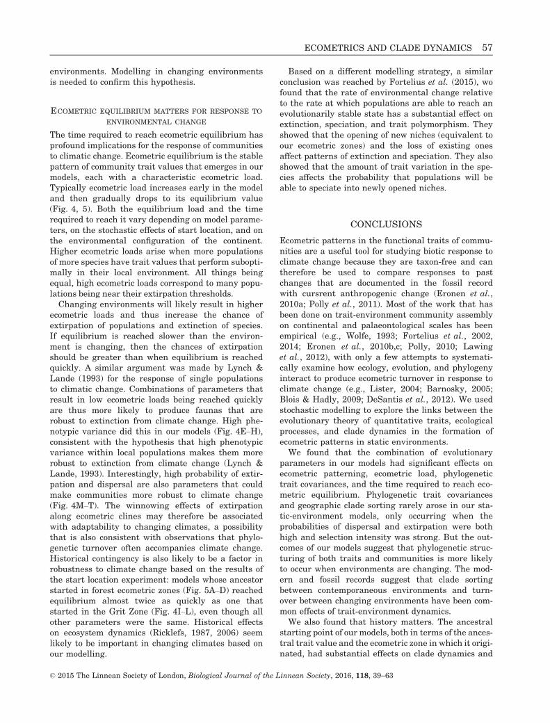
environments. Modelling in changing environmentsis needed to confirm this hypothesis.

ECOMETRIC EQUILIBRIUM MATTERS FOR RESPONSE TO

ENVIRONMENTAL CHANGE

The time required to reach ecometric equilibrium hasprofound implications for the response of communitiesto climatic change. Ecometric equilibrium is the stablepattern of community trait values that emerges in ourmodels, each with a characteristic ecometric load.Typically ecometric load increases early in the modeland then gradually drops to its equilibrium value(Fig. 4, 5). Both the equilibrium load and the timerequired to reach it vary depending on model parame-ters, on the stochastic effects of start location, and onthe environmental configuration of the continent.Higher ecometric loads arise when more populationsof more species have trait values that perform subopti-mally in their local environment. All things beingequal, high ecometric loads correspond to many popu-lations being near their extirpation thresholds.

Changing environments will likely result in higherecometric loads and thus increase the chance ofextirpation of populations and extinction of species.If equilibrium is reached slower than the environ-ment is changing, then the chances of extirpationshould be greater than when equilibrium is reachedquickly. A similar argument was made by Lynch &Lande (1993) for the response of single populationsto climatic change. Combinations of parameters thatresult in low ecometric loads being reached quicklyare thus more likely to produce faunas that arerobust to extinction from climate change. High phe-notypic variance did this in our models (Fig. 4E–H),consistent with the hypothesis that high phenotypicvariance within local populations makes them morerobust to extinction from climate change (Lynch &Lande, 1993). Interestingly, high probability of extir-pation and dispersal are also parameters that couldmake communities more robust to climate change(Fig. 4M–T). The winnowing effects of extirpationalong ecometric clines may therefore be associatedwith adaptability to changing climates, a possibilitythat is also consistent with observations that phylo-genetic turnover often accompanies climate change.Historical contingency is also likely to be a factor inrobustness to climate change based on the results ofthe start location experiment: models whose ancestorstarted in forest ecometric zones (Fig. 5A–D) reachedequilibrium almost twice as quickly as one thatstarted in the Grit Zone (Fig. 4I–L), even though allother parameters were the same. Historical effectson ecosystem dynamics (Ricklefs, 1987, 2006) seemlikely to be important in changing climates based onour modelling.

Based on a different modelling strategy, a similarconclusion was reached by Fortelius et al. (2015), wofound that the rate of environmental change relativeto the rate at which populations are able to reach anevolutionarily stable state has a substantial effect onextinction, speciation, and trait polymorphism. Theyshowed that the opening of new niches (equivalent toour ecometric zones) and the loss of existing onesaffect patterns of extinction and speciation. They alsoshowed that the amount of trait variation in the spe-cies affects the probability that populations will beable to speciate into newly opened niches.

CONCLUSIONS

Ecometric patterns in the functional traits of commu-nities are a useful tool for studying biotic response toclimate change because they are taxon-free and cantherefore be used to compare responses to pastchanges that are documented in the fossil recordwith cursrent anthropogenic change (Eronen et al.,2010a; Polly et al., 2011). Most of the work that hasbeen done on trait-environment community assemblyon continental and palaeontological scales has beenempirical (e.g., Wolfe, 1993; Fortelius et al., 2002,2014; Eronen et al., 2010b,c; Polly, 2010; Lawinget al., 2012), with only a few attempts to systemati-cally examine how ecology, evolution, and phylogenyinteract to produce ecometric turnover in response toclimate change (e.g., Lister, 2004; Barnosky, 2005;Blois & Hadly, 2009; DeSantis et al., 2012). We usedstochastic modelling to explore the links between theevolutionary theory of quantitative traits, ecologicalprocesses, and clade dynamics in the formation ofecometric patterns in static environments.

We found that the combination of evolutionaryparameters in our models had significant effects onecometric patterning, ecometric load, phylogenetictrait covariances, and the time required to reach eco-metric equilibrium. Phylogenetic trait covariancesand geographic clade sorting rarely arose in our sta-tic-environment models, only occurring when theprobabilities of dispersal and extirpation were bothhigh and selection intensity was strong. But the out-comes of our models suggest that phylogenetic struc-turing of both traits and communities is more likelyto occur when environments are changing. The mod-ern and fossil records suggest that clade sortingbetween contemporaneous environments and turn-over between changing environments have been com-mon effects of trait-environment dynamics.

We also found that history matters. The ancestralstarting point of our models, both in terms of the ances-tral trait value and the ecometric zone in which it origi-nated, had substantial effects on clade dynamics and



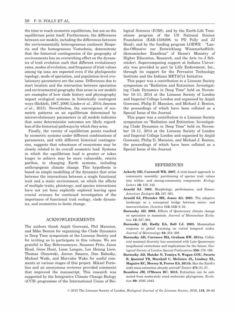
the time to reach ecometric equilibrium, but not on theequilibrium point itself. Furthermore, the differencesbetween our models, including the differences betweenthe environmentally heterogeneous continent Hespe-ria and the homogeneous Vostochnia, demonstratethat the historical contingencies of the geography ofenvironments has an overarching effect on the dynam-ics of trait evolution such that different evolutionaryrates, modes of evolution, and frequency of trait valuesamong tip taxa are expected even if the phylogenetictopology, mode of speciation, and population-level evo-lutionary parameters are the same. Differences due tostart location and the interaction between speciationand environmental geography that arose in our modelsare examples of how clade history and physiographyimpact ecological systems in historically contingentways (Ricklefs, 1987, 2006; Linder et al., 2014; Jønssonet al., 2015). Nevertheless, the convergence of eco-metric patterns on an equilibrium determined bymicroevolutionary parameters in all models indicatesthat some deterministic outcomes are likely regard-less of the historical pathways by which they arise.

Finally, the variety of equilibrium points reachedby ecometric systems under different combinations ofparameters, and with different historical contingen-cies, suggests that robustness of ecosystems may beclosely related to its overall ecometric load. Systemsin which the equilibrium load is greater or takeslonger to achieve may be more vulnerable, ceterisparibus, to changing Earth systems, includinganthropogenic climate change. This hypothesis isbased on simple modelling of the dynamics that arisebetween the interactions between a single functionaltrait and a static environment, on which the effectsof multiple traits, pleiotropy, and species interactionshave not yet been explicitly explored leaving opencrucial avenues for continued investigation of theimportance of functional trait ecology, clade dynam-ics, and ecometrics to biotic change.

ACKNOWLEDGEMENTS

The authors thank Anjali Goswami, Phil Mannion,and Mike Benton for organizing the Clade Dynamicsin Deep Time symposium at the Linnean Society andfor inviting us to participate in this volume. We aregrateful to Kay Behrensmeyer, Susanne Fritz, JasonHead, Gene Hunt, Liam Langan, Lee Hsiang Liow,Thomas Olszewski, Jereon Smaers, Dan Rabosky,Michael Wade, and Marvalee Wake for useful com-ments at various stages of this project. Mikael Forte-lius and an anonymous reviewer provided commentsthat improved the manuscript. This research wassupported by the Integrative Climate Change Biology(iCCB) programme of the International Union of Bio-

logical Sciences (IUBS), and by the Earth-Life Tran-sitions program of the US National ScienceFoundation (EAR-1338298, to PD Polly and JJHead), and by the funding program LOEWE – “Lan-des-Offensive zur Entwicklung Wissenschaftlich-€okonomischer Exzellenz” of Hesse’s Ministry ofHigher Education, Research, and the Arts (to J Sch-nitzler). Supercomputing support at Indiana Univer-sity was provided in part by Lilly Endowment, Inc.,through its support for the Pervasive TechnologyInstitute and the Indiana METACyt Initiative.

This paper was a contribution to a Linnean Societysymposium on “Radiation and Extinction: Investigat-ing Clade Dynamics in Deep Time” held on Novem-ber 10–11, 2014 at the Linnean Society of Londonand Imperial College London and organised by AnjaliGoswami, Philip D. Mannion, and Michael J. Benton,the proceedings of which have been collated as aSpecial Issue of the Journal.

This paper was a contribution to a Linnean Societysymposium on “Radiation and Extinction: Investigat-ing Clade Dynamics in Deep Time” held on Novem-ber 10–11, 2014 at the Linnean Society of Londonand Imperial College London and organised by AnjaliGoswami, Philip D. Mannion, and Michael J. Benton,the proceedings of which have been collated as aSpecial Issue of the Journal.

REFERENCES

Ackerly DD, Cornwell WK. 2007. A trait-based approach to

community assembly: partitioning of species trait values

into within- and among-community components. Ecology

Letters 10: 135–145.

Arnold SJ. 1983. Morphology, performance, and fitness.

American Zoologist 23: 347–361.

Arnold SJ, Pfrender ME, Jones AG. 2001. The adaptive

landscape as a conceptual bridge between micro- and

macroevolution. Genetica 112–113: 9–32.

Barnosky AD. 2005. Effects of Quaternary climate change

on speciation in mammals. Journal of Mammalian Evolu-

tion 12: 247–264.

Barnosky AD, Hadly EA, Bell CJ. 2003. Mammalian

response to global warming on varied temporal scales.

Journal of Mammalogy 84: 354–368.

Barnosky AD, Carrasco MA, Graham RW. 2011a. Collat-

eral mammal diversity loss associated with Late Quaternary

megafaunal extinctions and implications for the future. Geo-

logical Society of London Special Publications 358: 179–189.

Barnosky AD, Matzke N, Tomiya S, Wogan GOU, Swartz

B, Quental TB, Marshall C, McGuire JL, Lindsey EL,

Maguire KC, Mersey B, Ferrer EA. 2011b.Has the Earth’s

sixth mass extinction already arrived?Nature 471: 51–57.

Beaulieu JM, O’Meara BC. 2015. Extinction can be esti-

mated from moderately sized molecular phylogenies. Evolu-

tion 69: 1036–1043.



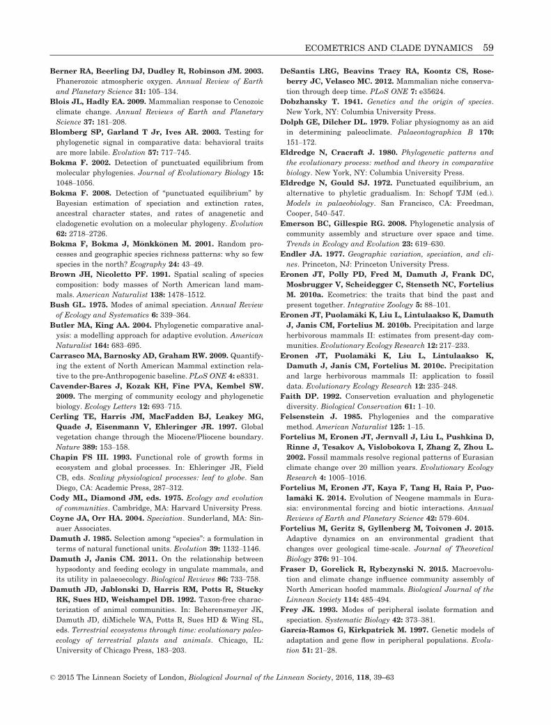
Berner RA, Beerling DJ, Dudley R, Robinson JM. 2003.

Phanerozoic atmospheric oxygen. Annual Review of Earth

and Planetary Science 31: 105–134.

Blois JL, Hadly EA. 2009. Mammalian response to Cenozoic

climate change. Annual Reviews of Earth and Planetary

Science 37: 181–208.

Blomberg SP, Garland T Jr, Ives AR. 2003. Testing for

phylogenetic signal in comparative data: behavioral traits

are more labile. Evolution 57: 717–745.

Bokma F. 2002. Detection of punctuated equilibrium from

molecular phylogenies. Journal of Evolutionary Biology 15:

1048–1056.

Bokma F. 2008. Detection of “punctuated equilibrium” by

Bayesian estimation of speciation and extinction rates,

ancestral character states, and rates of anagenetic and

cladogenetic evolution on a molecular phylogeny. Evolution

62: 2718–2726.

Bokma F, Bokma J, M€onkk€onen M. 2001. Random pro-

cesses and geographic species richness patterns: why so few

species in the north? Ecography 24: 43–49.

Brown JH, Nicoletto PF. 1991. Spatial scaling of species

composition: body masses of North American land mam-

mals. American Naturalist 138: 1478–1512.

Bush GL. 1975. Modes of animal speciation. Annual Review

of Ecology and Systematics 6: 339–364.

Butler MA, King AA. 2004. Phylogenetic comparative anal-

ysis: a modelling approach for adaptive evolution. American

Naturalist 164: 683–695.

Carrasco MA, Barnosky AD, Graham RW. 2009. Quantify-

ing the extent of North American Mammal extinction rela-

tive to the pre-Anthropogenic baseline. PLoS ONE 4: e8331.

Cavender-Bares J, Kozak KH, Fine PVA, Kembel SW.

2009. The merging of community ecology and phylogenetic

biology. Ecology Letters 12: 693–715.

Cerling TE, Harris JM, MacFadden BJ, Leakey MG,

Quade J, Eisenmann V, Ehleringer JR. 1997. Global

vegetation change through the Miocene/Pliocene boundary.

Nature 389: 153–158.

Chapin FS III. 1993. Functional role of growth forms in

ecosystem and global processes. In: Ehleringer JR, Field

CB, eds. Scaling physiological processes: leaf to globe. San

Diego, CA: Academic Press, 287–312.

Cody ML, Diamond JM, eds. 1975. Ecology and evolution

of communities. Cambridge, MA: Harvard University Press.

Coyne JA, Orr HA. 2004. Speciation. Sunderland, MA: Sin-

auer Associates.

Damuth J. 1985. Selection among “species”: a formulation in

terms of natural functional units. Evolution 39: 1132–1146.

Damuth J, Janis CM. 2011. On the relationship between

hypsodonty and feeding ecology in ungulate mammals, and

its utility in palaeoecology. Biological Reviews 86: 733–758.

Damuth JD, Jablonski D, Harris RM, Potts R, Stucky

RK, Sues HD, Weishampel DB. 1992. Taxon-free charac-

terization of animal communities. In: Beherensmeyer JK,

Damuth JD, diMichele WA, Potts R, Sues HD & Wing SL,

eds. Terrestrial ecosystems through time: evolutionary paleo-

ecology of terrestrial plants and animals. Chicago, IL:

University of Chicago Press, 183–203.

DeSantis LRG, Beavins Tracy RA, Koontz CS, Rose-

berry JC, Velasco MC. 2012. Mammalian niche conserva-

tion through deep time. PLoS ONE 7: e35624.

Dobzhansky T. 1941. Genetics and the origin of species.

New York, NY: Columbia University Press.

Dolph GE, Dilcher DL. 1979. Foliar physiognomy as an aid

in determining paleoclimate. Palaeontographica B 170:

151–172.

Eldredge N, Cracraft J. 1980. Phylogenetic patterns and

the evolutionary process: method and theory in comparative

biology. New York, NY: Columbia University Press.

Eldredge N, Gould SJ. 1972. Punctuated equilibrium, an

alternative to phyletic gradualism. In: Schopf TJM (ed.).

Models in palaeobiology. San Francisco, CA: Freedman,

Cooper, 540–547.

Emerson BC, Gillespie RG. 2008. Phylogenetic analysis of

community assembly and structure over space and time.

Trends in Ecology and Evolution 23: 619–630.

Endler JA. 1977. Geographic variation, speciation, and cli-

nes. Princeton, NJ: Princeton University Press.

Eronen JT, Polly PD, Fred M, Damuth J, Frank DC,

Mosbrugger V, Scheidegger C, Stenseth NC, Fortelius

M. 2010a. Ecometrics: the traits that bind the past and

present together. Integrative Zoology 5: 88–101.

Eronen JT, Puolam€aki K, Liu L, Lintulaakso K, Damuth

J, Janis CM, Fortelius M. 2010b. Precipitation and large

herbivorous mammals II: estimates from present-day com-

munities. Evolutionary Ecology Research 12: 217–233.

Eronen JT, Puolam€aki K, Liu L, Lintulaakso K,

Damuth J, Janis CM, Fortelius M. 2010c. Precipitation

and large herbivorous mammals II: application to fossil

data. Evolutionary Ecology Research 12: 235–248.

Faith DP. 1992. Conservetion evaluation and phylogenetic

diversity. Biological Conservation 61: 1–10.

Felsenstein J. 1985. Phylogenies and the comparative

method. American Naturalist 125: 1–15.

Fortelius M, Eronen JT, Jernvall J, Liu L, Pushkina D,

Rinne J, Tesakov A, Vislobokova I, Zhang Z, Zhou L.

2002. Fossil mammals resolve regional patterns of Eurasian

climate change over 20 million years. Evolutionary Ecology

Research 4: 1005–1016.

Fortelius M, Eronen JT, Kaya F, Tang H, Raia P, Puo-

lam�aki K. 2014. Evolution of Neogene mammals in Eura-

sia: environmental forcing and biotic interactions. Annual

Reviews of Earth and Planetary Science 42: 579–604.

Fortelius M, Geritz S, Gyllenberg M, Toivonen J. 2015.

Adaptive dynamics on an environmental gradient that

changes over geological time-scale. Journal of Theoretical

Biology 376: 91–104.

Fraser D, Gorelick R, Rybczynski N. 2015. Macroevolu-

tion and climate change influence community assembly of

North American hoofed mammals. Biological Journal of the

Linnean Society 114: 485–494.

Frey JK. 1993. Modes of peripheral isolate formation and

speciation. Systematic Biology 42: 373–381.

Garc�ıa-Ramos G, Kirkpatrick M. 1997. Genetic models of

adaptation and gene flow in peripheral populations. Evolu-

tion 51: 21–28.



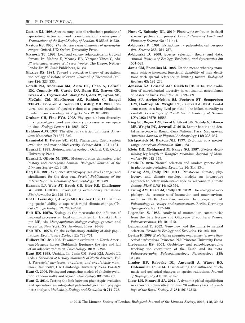
Gaston KJ. 1998. Species-range size distributions: products of

speciation, extinction and transformation. Philosophical

Transactions of the Royal Society of London, B 353: 219–230.

Gaston KJ. 2003. The structure and dynamics of geographic

ranges. Oxford, UK: Oxford University Press.

Givnesh TJ. 1984. Leaf and canopy adaptations in tropical

forests. In: Medina E, Mooney HA, V�azquez-Y�anes C, eds.

Physiological ecology of the wet tropics. The Hague, Nether-

lands: Dr. W. Junk Publishers, 51–84.

Glazier DS. 1987. Toward a predictive theory of speciation:

the ecology of isolate selection. Journal of Theoretical Biol-

ogy 126: 323–333.

Gotelli NJ, Anderson MJ, Arita HT, Chao A, Colwell

RK, Connolly SR, Currie DJ, Dunn RR, Graves GR,

Green JL, Grytnes J-A, Jiang Y-H, Jetz W, Lyons SK,

McCain CM, MacGurran AE, Rahbek C, Rangel

TFLVB, Sober�on J, Webb CO, Willig MR. 2009. Pat-

terns and causes of species richness: a general simulation

model for macroecology. Ecology Letters 12: 873–886.

Graham CH, Fine PVA. 2008. Phylogenetic beta diversity:

linking ecological and evolutionary processes across space

in time. Ecology Letters 11: 1265–1277.

Haldane JBS. 1937. The effect of variation on fitness. Amer-

ican Naturalist 71: 337–349.

Hannisdal B, Peters SE. 2011. Phanerozoic Earth system

evolution and marine biodiversity. Science 334: 1121–1124.

Hanski I. 1999. Metapopulation ecology. Oxford, UK: Oxford

University Press.

Hanski I, Gilpin M. 1991. Metapopulation dynamics: brief

history and conceptual domain. Biological Journal of the

Linnean Society 42: 3–16.

Haq BU. 1991. Sequence stratigraphy, sea-level change, and

significance for the deep sea. Special Publications of the

International Association of Sedimentology 12: 3–39.

Harmon LJ, Weir JT, Brock CD, Glor RE, Challenger

W. 2008. GEIGER: investigating evolutionary radiations.

Bioinformatics 24: 129–131.

Hof C, Levinsky I, Ara�ujo MB, Rahbek C. 2011. Rethink-

ing species’ ability to cope with rapid climate change. Glo-

bal Change Biology 17: 2987–2990.

Holt RD. 1997a. Ecology at the mesoscale: the influence of

regional processes on local communities. In: Hanski I, Gil-

pin ME, eds. Metapopulation biology: ecology, genetics and

evolution. New York, NY: Academic Press, 76–88.

Holt RD. 1997b. On the evolutionary stability of sink popu-

lations. Evolutionary Ecology 11: 723–731.

Hulbert RC Jr. 1993. Taxonomic evolution in North Ameri-

can Neogene horses (Subfamily Equinae): the rise and fall

of an adaptive radiation. Paleobiology 19: 216–234.

Hunt RM 1998. Ursidae. In: Janis CM, Scott KM, Jacobs LL

(eds.), Evolution of tertiary mammals of North America. Vol.

1: Terrestrial carnivores, ungulates, and ungulatelike mam-

mals. Cambridge, UK: Cambridge University Press. 174–189

Hunt G. 2006. Fitting and comparing models of phyletic evolu-

tion: random walks and beyond. Paleobiology 32: 578–601.

Hunt G. 2014. Testing the link between phenotypic evolution

and speciation: an integrated palaeontological and phyloge-

netic analysis. Methods in Ecology and Evolution 4: 714–723.

Hunt G, Rabosky DL. 2010. Phenotypic evolution in fossil

species: pattern and process. Annual Review of Earth and

Planetary Science 42: 421–441.

Jablonski D. 1991. Extinctions: a paleontological perspec-

tive. Science 253: 754–757.

Jablonski D. 2008. Species selection: theory and data.

Annual Reviews of Ecology, Evolution, and Systematics 39:

501–524.

Janis CM, Fortelius M. 1988. On the means whereby mam-

mals achieve increased functional durability of their denti-

tions with special reference to limiting factors. Biological

Reviews 63: 197–230.

Jønsson KA, Lessard J-P, Ricklefs RE. 2015. The evolu-

tion of morphological diversity in continental assemblages

of passerine birds. Evolution 69: 879–889.

King SJ, Arrigo-Nelson SJ, Pochron ST, Semprebon

GM, Godfrey LR, Wright PC, Jernvall J. 2004. Dental

senescence in a long-lived primate links infant mortality to

rainfall. Proceedings of the National Academy of Science

USA 102: 16579–16583.

King SJ, Boyer DM, Tecot S, Strait SG, Zohdy S, Blanco

MB, Wright PC, Jernvall J. 2012. Lemur habitat and den-

tal senescence in Ranomafana National Park, Madagascar.

American Journal of Physical Anthropology 148: 228–237.

Kirkpatrick M, Barton NH. 1997. Evolution of a species’

range. American Naturalist 150: 1–23.

Klein DR, Meldgaard M, Fancy SG. 1987. Factors deter-

mining leg length in Rangifer tarandus. Journal of Mam-

malogy 68: 642–655.

Lande R. 1976. Natural selection and random genetic drift

in phenotypic evolution. Evolution 30: 314–334.

Lawing AM, Polly PD. 2011. Pleistocene climate, phy-

logeny, and climate envelope models: an integrative

approach to better understand species’ response to climate

change. PLoS ONE 16: e28554.

Lawing AM, Head JJ, Polly PD. 2012. The ecology of mor-

phology: the ecometrics of locomotion and macroenviron-

ment in North American snakes. In: Louys J, ed.

Paleontology in ecology and conservation. Berlin, Germany:

Springer-Verlag, 117–146.

Legendre S. 1986. Analysis of mammalian communities

from the Late Eocene and Oligocene of southern France.

Palaeovertebrata 16: 191–212.

Lenormand T. 2002. Gene flow and the limits to natural

selection. Trends in Ecology and Evolution 17: 183–189.

Levins R. 1968. Evolution in changing environments: some theo-

retical explorations. Princeton, NJ: Princeton University Press.

Lieberman BS. 2005. Geobiology and paleobiogeography:

tracking the coevolution of the Earth and its biota.

Palaeogeography, Palaeoclimatology, Palaeoecology 219:

23–33.

Linder HP, Rabosky DL, Antonelli A, W€uest RO,

Ohlem€uller R. 2014. Disentangling the influence of cli-

matic and geological changes on species radiations. Journal

of Biogeography 41: 1313–1325.

Liow LH, Finarelli JA. 2014. A dynamic global equilibrium

in carnivoran diversification over 20 million years. Proceed-

ings of the Royal Society, B 281: 20132312.



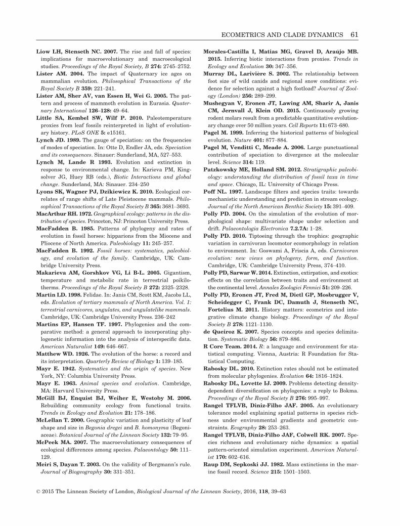
Liow LH, Stenseth NC. 2007. The rise and fall of species:

implications for macroevolutionary and macroecological

studies. Proceedings of the Royal Society, B 274: 2745–2752.

Lister AM. 2004. The impact of Quaternary ice ages on

mammalian evolution. Philosophical Transactions of the

Royal Society B 359: 221–241.

Lister AM, Sher AV, van Essen H, Wei G. 2005. The pat-

tern and process of mammoth evolution in Eurasia. Quater-

nary International 126–128: 49–64.

Little SA, Kembel SW, Wilf P. 2010. Paleotemperature

proxies from leaf fossils reinterpreted in light of evolution-

ary history. PLoS ONE 5: e15161.

Lynch JD. 1989. The gauge of speciation: on the frequencies

of modes of speciation. In: Otte D, Endler JA, eds. Speciation

and its consequences. Sinauer: Sunderland, MA, 527–553.

Lynch M, Lande R 1993. Evolution and extinction in

response to environmental change. In: Karieva PM, King-

solver JG, Huey RB (eds.), Biotic Interactions and global

change. Sunderland, MA: Sinauer. 234–250

Lyons SK, Wagner PJ, Dzikiewicz K. 2010. Ecological cor-

relates of range shifts of Late Pleistocene mammals. Philo-

sophical Transactions of the Royal Society B 365: 3681–3693.

MacArthur RH. 1972. Geographical ecology: patterns in the dis-

tribution of species. Princeton, NJ: Princeton University Press.

MacFadden B. 1985. Patterns of phylogeny and rates of

evolution in fossil horses: hipparions from the Miocene and

Pliocene of North America. Paleobiology 11: 245–257.

MacFadden B. 1992. Fossil horses: systematics, paleobiol-

ogy, and evolution of the family. Cambridge, UK: Cam-

bridge University Press.

Makarieva AM, Gorshkov VG, Li B-L. 2005. Gigantism,

temperature and metabolic rate in terrestrial poikilo-

therms. Proceedings of the Royal Society B 272: 2325–2328.

Martin LD. 1998. Felidae. In: Janis CM, Scott KM, Jacobs LL,

eds. Evolution of tertiary mammals of North America. Vol. 1:

terrestrial carnivores, ungulates, and ungulatelike mammals.

Cambridge, UK: Cambridge University Press. 236–242

Martins EP, Hansen TF. 1997. Phylogenies and the com-

parative method: a general approach to incorporating phy-

logenetic information into the analysis of interspecific data.

American Naturalist 149: 646–667.

Matthew WD. 1926. The evolution of the horse: a record and

its interpretation. Quarterly Review of Biology 1: 139–185.

Mayr E. 1942. Systematics and the origin of species. New

York, NY: Columbia University Press.

Mayr E. 1963. Animal species and evolution. Cambridge,

MA: Harvard University Press.

McGill BJ, Enquist BJ, Weiher E, Westoby M. 2006.

Rebuilding community ecology from functional traits.

Trends in Ecology and Evolution 21: 178–186.

McLellan T. 2000. Geographic variation and plasticity of leaf

shape and size in Begonia dregei and B. homonyma (Begoni-

aceae). Botanical Journal of the Linnean Society 132: 79–95.

McPeek MA. 2007. The macroevolutionary consequences of

ecological differences among species. Palaeontology 50: 111–

129.

Meiri S, Dayan T. 2003. On the validity of Bergmann’s rule.

Journal of Biogeography 30: 331–351.

Morales-Castilla I, Matias MG, Gravel D, Ara�ujo MB.

2015. Inferring biotic interactions from proxies. Trends in

Ecology and Evolution 30: 347–356.

Murray DL, Larivi�ere S. 2002. The relationship between

foot size of wild canids and regional snow conditions: evi-

dence for selection against a high footload? Journal of Zool-

ogy (London) 256: 289–299.

Mushegyan V, Eronen JT, Lawing AM, Sharir A, Janis

CM, Jernvall J, Klein OD. 2015. Continuously growing

rodent molars result from a predictable quantitative evolution-

ary change over 50 million years. Cell Reports 11: 673–680.

Pagel M. 1999. Inferring the historical patterns of biological

evolution. Nature 401: 877–884.

Pagel M, Venditti C, Meade A. 2006. Large punctuational

contribution of speciation to divergence at the molecular

level. Science 314: 119.

Patzkowsky ME, Holland SM. 2012. Stratigraphic paleobi-

ology: understanding the distribution of fossil taxa in time

and space. Chicago, IL: University of Chicago Press.

Poff NL. 1997. Landscape filters and species traits: towards

mechanistic understanding and prediction in stream ecology.

Journal of the North American Benthic Society 15: 391–409.

Polly PD. 2004. On the simulation of the evolution of mor-

phological shape: multivariate shape under selection and

drift. Palaeontologia Electronica 7.2.7A: 1–28.

Polly PD. 2010. Tiptoeing through the trophics: geographic

variation in carnivoran locomotor ecomorphology in relation

to environment. In: Goswami A, Friscia A, eds. Carnivoran

evolution: new views on phylogeny, form, and function.

Cambridge, UK: Cambridge University Press, 374–410.

Polly PD, SarwarW. 2014.Extinction, extirpation, and exotics:

effects on the correlation between traits and environment at

the continental level. Annales Zoologici Fennici 51: 209–226.

Polly PD, Eronen JT, Fred M, Dietl GP, Mosbrugger V,

Scheidegger C, Frank DC, Damuth J, Stenseth NC,

Fortelius M. 2011. History matters: ecometrics and inte-

grative climate change biology. Proceedings of the Royal

Society B 278: 1121–1130.

de Queiroz K. 2007. Species concepts and species delimita-

tion. Systematic Biology 56: 879–886.

R Core Team. 2014. R: a language and environment for sta-

tistical computing. Vienna, Austria: R Foundation for Sta-

tistical Computing.

Rabosky DL. 2010. Extinction rates should not be estimated

from molecular phylogenies. Evolution 64: 1816–1824.

Rabosky DL, Lovette IJ. 2009. Problems detecting density-

dependent diversification on phylogenies: a reply to Bokma.

Proceedings of the Royal Society B 276: 995–997.

Rangel TFLVB, Diniz-Filho JAF. 2005. An evolutionary

tolerance model explaining spatial patterns in species rich-

ness under environmental gradients and geometric con-

straints. Ecography 28: 253–263.

Rangel TFLVB, Diniz-Filho JAF, Colwell RK. 2007. Spe-

cies richness and evolutionary niche dynamics: a spatial

pattern-oriented simulation experiment. American Natural-

ist 170: 602–616.

Raup DM, Sepkoski JJ. 1982. Mass extinctions in the mar-

ine fossil record. Science 215: 1501–1503.



Revell LJ, Harmon LJ, Collar DC. 2008. Phylogenetic sig-

nal, evolutionary process, and rate. Systematic Biology 57:

591–601.

Ricklefs RE. 1987. Community diversity: relative roles of

local and regional processes. Science 235: 167–171.

Ricklefs RE. 2006. Evolutionary diversification and the ori-

gin of the diversity-environment relationship. Ecology 87:

S3–S13.

Ricklefs RE, Travis J. 1980. A morphological approach to the

study of Avian community organization. Auk 97: 321–338.

Roy K, Goldberg EE. 2007. Origination, extinction, and dis-

persal: integrative models for understanding present-day

diversity gradients. American Naturalist 170: S71–S85.

Silvestro D, Schnitzler J, Zizka G. 2011. A Bayesian frame-

work to estimate diversification rates and their variation

through time and space. BMC Evolutionary Biology 11: 311.

Simpson GG. 1944. Tempo and mode in evolution. New

York, NY: Columbia University Press.

Tedford RH, Wang X, Taylor BE. 2009. Phylogenetic sys-

tematics of the North American fossil Caninae (Carnivora:

Canidae). Bulletin of the American Museum of Natural His-

tory 325: 1–218.

Violle C, Reich PB, Pacala SW, Enquist BJ, Kattge J.

2014. The emergence and promise of functional biogeogra-

phy. Proceedings of the National Academy of Sciences USA

38: 13690–13696.

Voorhies MR. 1969. Taphonomy and population dynamics of

an early Pliocene vertebrate fauna, Knox County,

Nebraska. Rocky Mountain Geology 8: 1–69.

Vrba ES 1993. Turnover-pulses, the Red Queen, and related

topics. American Journal of Science 293-A: 418–452.

Vrba ES. 1995. The fossil record of African antelopes (Mam-

malia, Bovidae) in relation to human evolution and paleocli-

mate. In: Vrba ES, Denton GH, Partridge TC, Burckle LH,

eds. Paleoclimate and evolution with emphasis of human

origins. New Haven, CT: Yale University Press, 383–424.

Vrba ES, DeGusta D. 2004. Do species populations really

start small? New perspectives from the Late Neogene fossil

record of African mammals. Philosophical Transactions of

the Royal Society of London, B 359: 285–293.

Webb CO. 2000. Exploring the phylogenetic structure of eco-

logical communities: an example for rain forest trees. Amer-

ican Naturalist 156: 145–155.

Webb T III, Bartlein PJ. 1992.Global changes during the last

three million years: climatic controls and biotic responses.

Annual Review of Ecology and Systematics 23: 141–173.

Webb CO, Ackerly DD, McPeek MA, Donoghue MJ.

2002. Phylogenies and community ecology. Annual Review

of Ecology and Systematics 33: 475–505.

Webb CT, Hoeting JA, Ames GM, Pyne MI, Poff NL.

2010. A structured and dynamic framework to advance

traits-based theory and prediction in ecology. Ecology Let-

ters 13: 267–283.

West-Eberhard MJ. 1989. Phenotypic plasticity and the ori-

gin of diversity. Annual Review of Ecology and Systematics

20: 249–278.

Westoby M, Leishman MR, Lord JM. 1995. On misinter-

preting the ‘phylogenetic correlation’. Journal of Ecology

83: 531–534.

Whittaker RH. 1967. Gradient analysis of vegetation. Bio-

logical Reviews 49: 207–264.

Whittaker RH. 1975. Communities and ecosystems. New

York, NY: MacMillan Publishing.

Willis KJ, MacDonald GM. 2011. Long-term ecological

records and their relevance to climate change predictions

for a warmer world. Annual Review of Ecology, Evolution,

and Systematics 42: 267–287.

Wolf D, Bernor RL, Hussain ST. 2013. A systematic, bios-

tratigraphic, and paleobiogeographic reevaluation of the

Siwalik hipparionine horse assemblage from the Potwar

Plateau, northern Pakistan. Palaeontographica A: Paleozo-

ology-Stratigraphy 300: 1–115.

Wolfe JA. 1993. A method of obtaining climatic parameters

from leaf assemblages. Bulletin of the US Geological Survey

2040: 1–71.

Wright IJ, Reich PB, Cornelissen HC, Falster DS, Gar-

ier E, Hikosaka K, Lamont BB, Lee W, Oleksyn J,

Osada N, Poorter H, Villar R, Warton DI, Westoby M.

2005. Assessing the generality of global leaf trait relation-

ships. New Phytologist 166: 485–496.

SUPPORTING INFORMATION

Additional Supporting Information may be found online in the supporting information tab for this article:

Figures S1. S1.1 Geography of Humboldtland. S1.2 Phylogenetic community metrics.Figure S2. Ecometric equilibrium graphs.Figure S3. Phylogenetic occupation of ecometric zones.Table S1. Model output summary statistics.Table S2. Database of Humboldtland’s geography and environmentTable S3. Animated ecometric maps for models in Fig. 4.Table S4. Animated ecometric maps for models in Fig. 5.Data S1. Detailed explanation of the ecometric model and parameters.Data S2. Model output summary graphics.Data S3. Mathematica code for the ecometric model.



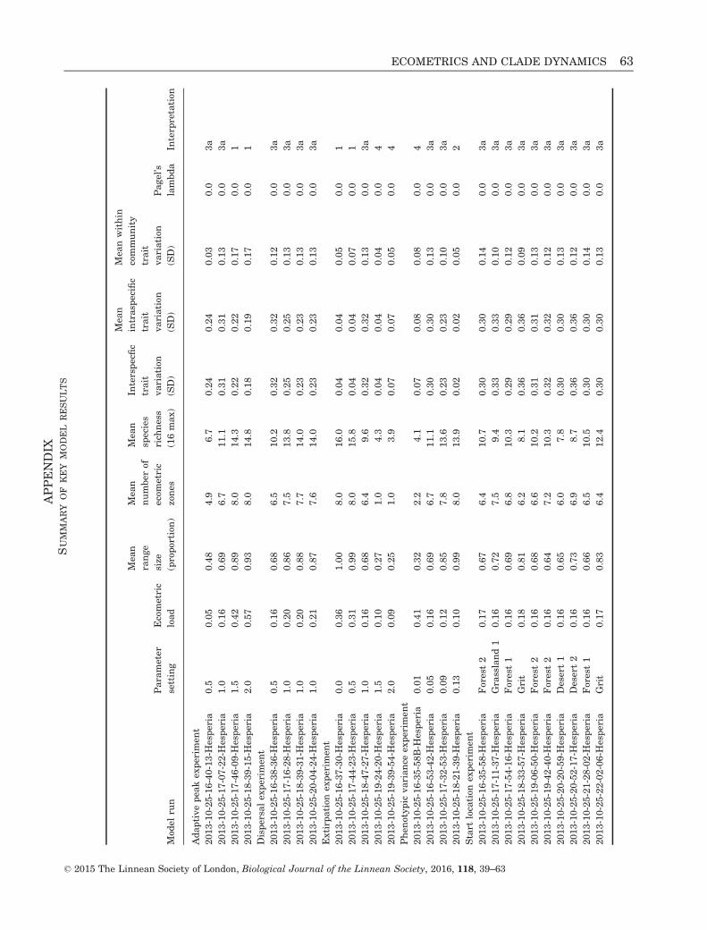
. Mod

elru

n

Parameter

setting

Ecometric

load

Mea

n

range

size

(proportion

)

Mea

n

number

of

ecom

etric

zones

Mea

n

species

rich

ness

(16max)

Interspecfic

trait

variation

(SD)

Mea

n

intrasp

ecific

trait

variation

(SD)

Mea

nwithin

community

trait

variation

(SD)

Pagel’s

lambda

Interp

retation

Adaptivepea

kex

perim

ent

2013-10-25-16-40-13-H

esperia

0.5

0.05

0.48

4.9

6.7

0.24

0.24

0.03

0.0

3a

2013-10-25-17-07-22-H

esperia

1.0

0.16

0.69

6.7

11.1

0.31

0.31

0.13

0.0

3a

2013-10-25-17-46-09-H

esperia

1.5

0.42

0.89

8.0

14.3

0.22

0.22

0.17

0.0

1

2013-10-25-18-39-15-H

esperia

2.0

0.57

0.93

8.0

14.8

0.18

0.19

0.17

0.0

1

Dispersa

lex

perim

ent

2013-10-25-16-38-36-H

esperia

0.5

0.16

0.68

6.5

10.2

0.32

0.32

0.12

0.0

3a

2013-10-25-17-16-28-H

esperia

1.0

0.20

0.86

7.5

13.8

0.25

0.25

0.13

0.0

3a

2013-10-25-18-39-31-H

esperia

1.0

0.20

0.88

7.7

14.0

0.23

0.23

0.13

0.0

3a

2013-10-25-20-04-24-H

esperia

1.0

0.21

0.87

7.6

14.0

0.23

0.23

0.13

0.0

3a

Extirp

ation

experim

ent

2013-10-25-16-37-30-H

esperia

0.0

0.36

1.00

8.0

16.0

0.04

0.04

0.05

0.0

1

2013-10-25-17-44-23-H

esperia

0.5

0.31

0.99

8.0

15.8

0.04

0.04

0.07

0.0

1

2013-10-25-18-47-27-H

esperia

1.0

0.16

0.68

6.4

9.6

0.32

0.32

0.13

0.0

3a

2013-10-25-19-24-20-H

esperia

1.5

0.10

0.27

1.0

4.3

0.04

0.04

0.04

0.0

4

2013-10-25-19-39-54-H

esperia

2.0

0.09

0.25

1.0

3.9

0.07

0.07

0.05

0.0

4

Phen

otypic

variance

experim

ent

2013-10-25-16-35-58B-H

esperia

0.01

0.41

0.32

2.2

4.1

0.07

0.08

0.08

0.0

4

2013-10-25-16-53-42-H

esperia

0.05

0.16

0.69

6.7

11.1

0.30

0.30

0.13

0.0

3a

2013-10-25-17-32-53-H

esperia

0.09

0.12

0.85

7.8

13.6

0.23

0.23

0.10

0.0

3a

2013-10-25-18-21-39-H

esperia

0.13

0.10

0.99

8.0

13.9

0.02

0.02

0.05

0.0

2

Start

location

experim

ent

2013-10-25-16-35-58-H

esperia

Forest2

0.17

0.67

6.4

10.7

0.30

0.30

0.14

0.0

3a

2013-10-25-17-11-37-H

esperia

Grassland1

0.16

0.72

7.5

9.4

0.33

0.33

0.10

0.0

3a

2013-10-25-17-54-16-H

esperia

Forest1

0.16

0.69

6.8

10.3

0.29

0.29

0.12

0.0

3a

2013-10-25-18-33-57-H

esperia

Grit

0.18

0.81

6.2

8.1

0.36

0.36

0.09

0.0

3a

2013-10-25-19-06-50-H

esperia

Forest2

0.16

0.68

6.6

10.2

0.31

0.31

0.13

0.0

3a

2013-10-25-19-42-40-H

esperia

Forest2

0.16

0.64

7.2

10.3

0.32

0.32

0.12

0.0

3a

2013-10-25-20-20-59-H

esperia

Desert1

0.16

0.65

6.0

7.8

0.30

0.30

0.13

0.0

3a

2013-10-25-20-52-17-H

esperia

Desert2

0.16

0.73

6.9

8.7

0.36

0.36

0.12

0.0

3a

2013-10-25-21-28-02-H

esperia

Forest1

0.16

0.66

6.5

10.5

0.30

0.30

0.14

0.0

3a

2013-10-25-22-02-06-H

esperia

Grit

0.17

0.83

6.4

12.4

0.30

0.30

0.13

0.0

3a

APPENDIX

SUMMARY

OF

KEY

MODEL

RESULTS



Documents

Polly et al., 2016, Ecometric Modelling and Clade Dynamics