Pollution taxes and ·tradable emission permits:

Theory into practice

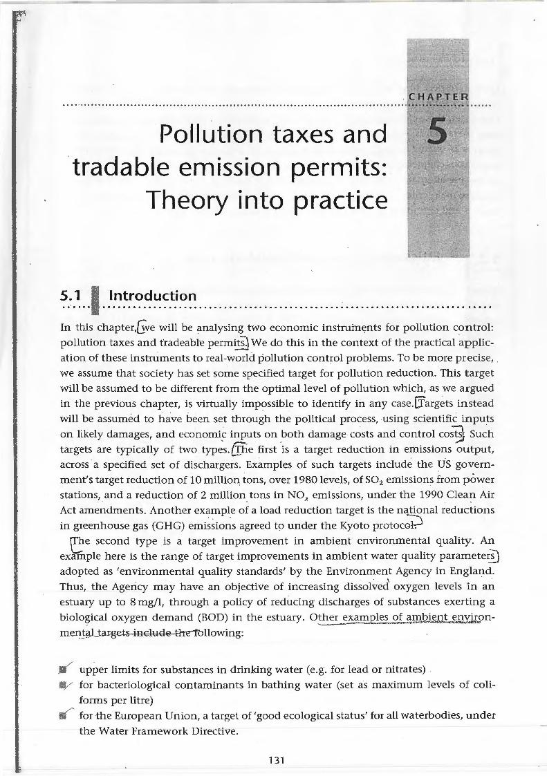
5.1 Introduction .. ·. . . . . ............................................................................ . In this chapter,G,,e will be analysing two economic instruin~nts for pollution control:

pollution taxes and fradeable perm~ We do this in the context of the practical applic­

ation of these instruments to real-world pollution control problems. To be more precise, .

we assume that society has set some specified target for pollution reduction. This t arget

will be assumed to be different from the optimal level of pollution which, as we argued

in the previous chapter, is virtually impossible to identify in any case.[fargets instead

will be assumed to have been set through the political process, using scientific inputs

on likely damages, and economi~ inputs on both damage c~sts and control co~ Such targets are typically of two types.@ie first is a target reduction in emissions output,

across a specified set of dischargers. Examples of such targets include the US govern­

ment's target reduction of 10 million. tons, over 1980 levels, of S02 emissions from power stations, and a reduction of 2 million. tons in NOx emissions, under the 1990 Clean Air

Act amendments. Another example of a load reduction target is the national reductions

in greenhouse gas (GHG) emi~sions agreed to under the Kyoto protoc~

ee second type is a target improvement in ambient environmental quality. An

example here is the range of target improvements in ambient water quality paramete~

adopted as 'environmental quality standards' by the Environment Agency in England.

Thus, the Agericy may have an objective of increasing dissolved oxygen levels in an

estuary up to 8 mg/1, through a policy of reducing discharges of substances exerting a

biological oxygen demand (BOD) in the estuary. O~her ~~~a1E£_~~~.£.L~.ill.ill~.nLt !.1ilEs>n­men_!qlJ:arg.ets-iIK~--the'Tollowing:

~ upper limits for substances in drinking water (e.g. for lead or nitrates)

!tY for bacteriological contaminants in bathing water (set as maximum levels of coli­

forms per litre)

~ for the European Union, a target of 'good ecological status' for all waterbodies, under

the Water Framework Directive.

131

132 nvironm nt I economics

@ith resp t to any of these environm ntal objectives, an Environmental Protection

Ag ncy (EPA) has many potential poli y tools at its disposag As noted in the previous

hapter, th e can be classified into r gulatory mechanisms"s'uch as design and perform.­

an e standards; economic instruments; and voluntary approaches. In this chapter, th

focus is on the practical application of economic instruments. As also set out in the

previous chapter, there are many criteria against w.hich an EPA can judge the performanc

of these alter.natives. Here, the focus will be on efficiency, or social cost minimisation,

as the main criterion of interest, although we also comment on distributional effects of

taxes and permits ~nd on political acceptability and environmental performance.

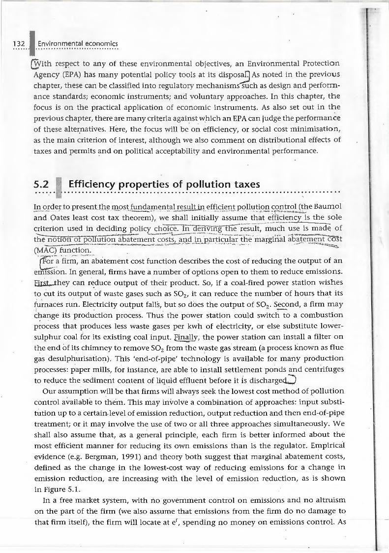
5.2 Efficiency properties of pollution taxes . . . . . . . ........................................................................... .

In order to presentJhe most fundamental result in efficient pollution control (the Baumol _ .... -- • .... - , ., ' " L •- • "• ' · · · - .:;. - ...... ..... . . ~·- ' ... ~ ... ._ .. '-. .. . -, .................. . 0 > ' 0 -• 0 • ••• , . ,, , -• • > L - ~ - · - - - ~ - - ... ..... , a: - , 11,; __,

and Oates least cost tax theorem), we shall initially assume that efficiency is the sole criterion used in deciding policy choTce:-rn:- aerivrffg-tn.Et resuit·; ··~uch use is mad~ of

- -- --·---•-"" lo,....,. ,,... . ... -'\"' - ·- · ~n-• ...,.,,., ''• __ __ .,_ ...... . ..-~ -• . -. d , • .-... ••- • • • I,'' '' <•- ~ ,..,_., •' .... / , , • .~ •.;" ,.... . ... , -,,,,.... ,.~ ~~

the ·oofforCorpollution abatement costsJ. ?P.,9-.i..9.: .Par.tic.u.~ar the marginal ab~te~~l:~. cost (MAC). ·fu-;;~ti~:-- -~~········ ... ,.,~~ ..... _~.,,,,·-... ,, ... - ''"''' ' ..... .. ' . . . ·,.. -~- ,. . -~-... :.-;.;- ·.:::-..

. ·-~.., ~- . ,•,· · ......... . .. .

(:.<:_:. a firm, an abatement cost function describes the cost of reducing the output of an

emission. In general, firms have a number of options open to them to reduce emissions.

Eir.s.t..J:hey can r~duce output of their product. So, if a coal-fired power station wishes to cut its output of waste gases such as S02 , it can reduce the number of hours that its

furnaces run. Ele~tricity output falls, but so does the output of S02 • Se<:9nd, a firm may

change its production process. Thus the power station could switch to a combustion

process that produces less waste gases per kwh of electricity, or else substitute lower­

sulphur coal for its existing coal input. f'in~'!!!Y, the power station can install a filter on the end of its chimney to remove S02 from the waste gas stream (a process known as flue

gas desulphurisation). This 'end-of-pipe' technology is available for many production

processes: paper mills, for instance, are able to install settlement ponds and centrifuges

to reduce the sediment content of liqu1d effluent before it is discharged.:) Our assumption will be that firms will always seek the lowest cost method of pollution

control a~ailable to them. This may involve a combination of approaches: input substi­

tution up to a certain level of emission reduction, output reduction and then end-of-pipe

treatment; or it may involve the use of two or all three approaches simultaneously. We

shall also assume that, as a general principle, each firm is better informed about the

most efficient manner for reducing its own emissions than is the regulator. Empirical

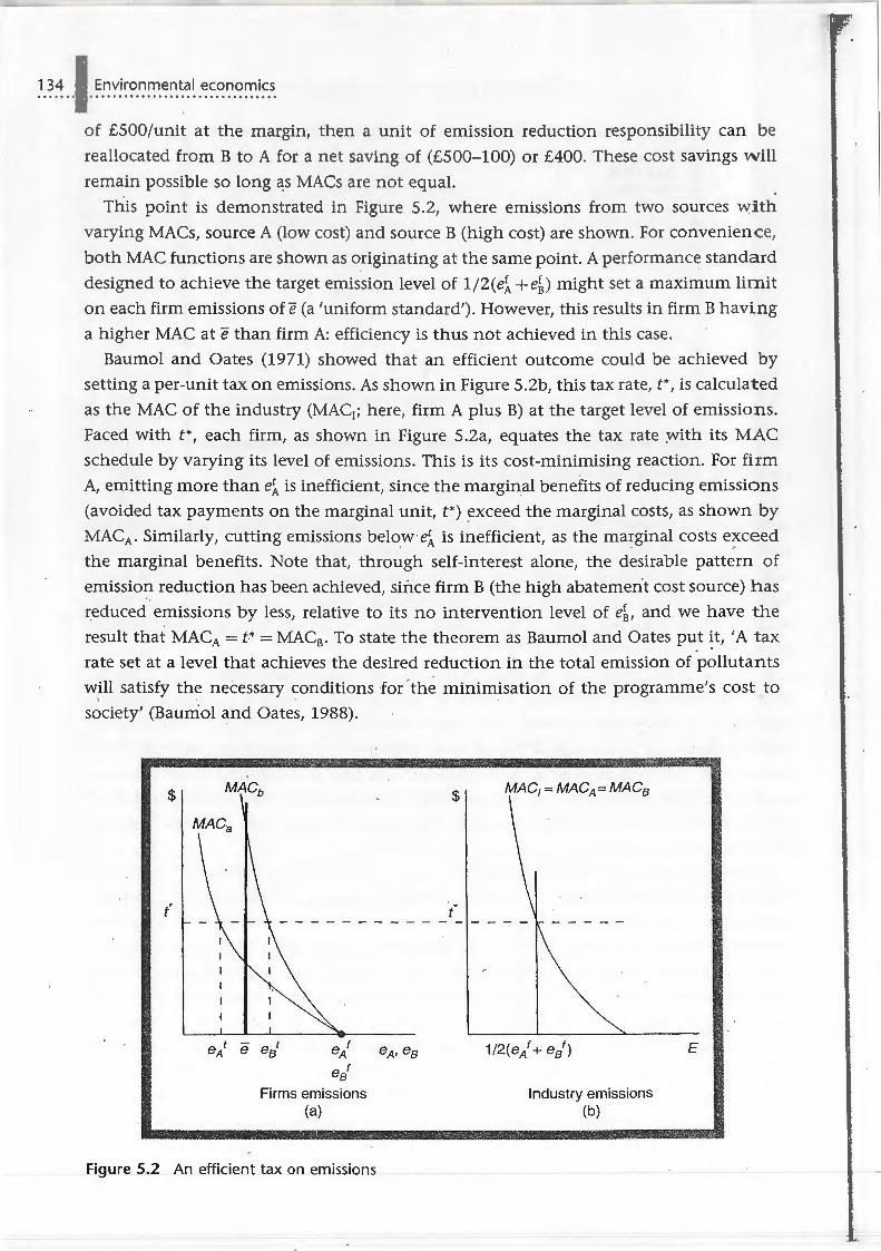
evidence (e.g. Bergman, 1991) and theory both suggest that marginal abatement costs,

defined as the change in the lowest-cost way of reducing emissions for a change in

emission reduction, are increasing with the level of emission reduction, as is shown

in Figure 5.1.

In a free market system, with no government control on emissions and no altruism

on the part of the firm (we also assume that emissions from the firm do no damage to

that firm itself), the firm will locate at ef, spending no money on emissions control. As

Marginal abatement costs (MAC)

MAC

Figure 5.1 Marg_inal abatement costs for a firm

. emissions, e e,

emissions are reduced, abatement costs rise at an increasing rate. Specifying a continu­

ously increasing MAC function is convenient analytically, since it implies that local

and global cost-minimising solutions will coincide. Some researchers have found that,

for some discharges, economies of scale are present in emissions treatment (e.g. Rowley et al. 1979). For the remainder of this chapter, however, we will assume continuously

increasing MAC functions. . '

It is also to be expected that MAC functions will vary across sources, for a given

pollutant. This means that some sources of, for example, BOD will find incremental

reductions in BOD output (much) less expensive than others, owing to differences in

plant location, age .an_d design; different production processes (distilling, paper making,

oil refining); differing levels of current emissions reduction, and differing levels of mana­

gerial knowledge and ability. For example, Hanley and Moffatt (1993) found that MACs

for direct discharges of BOD to the Forth Estuary in Scotland varied by as much as

thirtyfold across polluters.

The observation that MACs vary across sources is a key insight into why the cost­

minimi~ing means of securing a target reduction in aggregate emissions wiU involve

different amounts of emission reduction across sources. Assume for the present that a

uniformly mixed pollutant, such as a volatile organic compound (VOC), is the object of

control. Uniform mixing means that the target reduction in emissions is independent

of the source of emission, since a tonne less of discharge from any source in the control

area is equally effective in meeting a pollution reduction target as the same reduction

from any other source. It would seem sensible, in this situation, for high abatement

cost sources to reduce emissions by less than low abatement cost sources. In fact, a

necessary condition for an efficient solution in this case is that abatement costs, at the

margin, are equalised across all sources. This is proved formally below, but the intuition

is clear enough: if at the current allocation of emission reduction responsibility source

A can achieve a one-unit cut in VOCs at a cost of £100/unit, and source B faces a cost

134 Environmental economics

f £500/unit at the margin, th n a unit of emission reduction responsibility can b

r allocated from B to A for a n t saving of (£500- 100) or £400. Thes o t savings will

r main possible so long ~s MA s ar not equal.

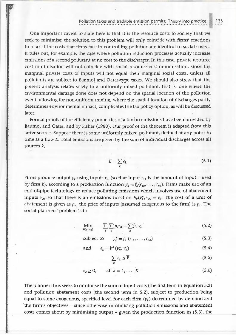
This point is demonstrated in Figure 5.2, where emissions from two sources vVi th

varying MACs, source A (low cost) and source B (high cost) are shown. For convenien

both MAC functions are shown as originating at the same point. A performance standard

designed to achieve the target emission level of 1/2(ei + eD might set a maximum limit

on each firm emissions of e (a 'uniform standard'). However, this results in firm B having

a higher MAC at e than firm A: efficiency is thus not achieved in this case.

Baumol and Oates (1971) showed that an efficient outcome could be achieved by

setting a per-unit tax on emissions. As shown in Figure 5.2b, this tax rate, t•, is calculat d

as the MAC of the industry (MAC1; here, firm A plus B) at the target level of emissions.

Faced with t•, each firm, as shown in Figure 5.2a, equates the tax rate :with its MA

schedule by varying its level of emissions. This is its cost-minimising reaction. For firm

A, emitting more than ei is inefficient, since the marginal benefits of reducing emissions

(avoided tax payments on the marginal unit, t•) ~xceed the marginal costs, as shown by

MACA. Similarly, cutting emissions belo_w ·ei is inefficient, as the marginal costs e~ceed

the marginal benefits. Note that, through self-interest alone, the desirable pattern of

emission reduction has been achieved, since firm B (the high abatemerit cost source) has

reduced emissions by less, relative to its no intervention level of eL and we have the

result that MACA = t* = MAC8 • To state the theorem as Baumol and Oates pu_t ~t, 'A tax

rate set at a level that achieves the desired reduction in the total emission of pollutants

will satisfy the necessary conditions for the minimisation of the programme's cost to

society' (Baumol and Oates, 1988).

$

(

ei ea'

Firms emissions (a)

Figure 5.2 An efficient tax on emissions

Industry emissions (b)

E

One important caveat t slat h re is that it is the res ur · sts to society that w

ek to minimise: the soluti n t this problem will only in id with firms' reacti n

to a tax if the costs that firms fa in controlling pollution ar identical to social costs -

it rules out, for example, th as where pollution reduction processes actually incr a ·

emissions of a second pollutan t at no cost to the discharger. In this case, private resour

cost minimisation will not oincide with social resource cost minimisation, since th.

marginal private costs of inputs will not equal their marginal social costs, unless all

pollutants are subject to Baumol and Oates-type taxes. We should also stress that th

present analysis relates solely to a uniformly mixed pollutant, that is, one where th

environmental damage done does not depend on the spatial location of the pollution

event: allowing for non-uniform mixing, where the spatial location of discharges partly

determines environmental impact, complicates the tax policy option, as will be discussed

later.

Formal proofs of the efficiency properties of a tax bn emissions have been provided by

Baumol and Oates, and by Fisher (1980) . Our proof of the theorem is adapted from this

latter source. Suppose there is some uniformly mixed pollutant, defined at any point in

time as a flow E. Total emissions are given by the sum of individual discharges across all

sources k,

(5.1)

Firms produce output Yk using inputs r;k (so that input rlk is the amount of input 1 used

by firm k), according to a production function Yk = f,/rlk, ... , r11k). Firms make use of an

end-of-pipe technology to reduce polluting emissions which involves use of abatement

inputs vk, . so that there is an emissions function bk(Yk, vk) = ek. Th~ cost of a unit of

abatement is given as Pv, the price of inputs (assumed exogenous to the firm) is Pi· The social planners' problem is to

L LP;T;k + LPv Vk . i k k

subject to

and ek = bk (Yk, vk)

I:ek::: E k

all k = l, ... ,K

(5.2)

(5.3)

(5.4)

(5.5)

(5.6)

The planner thus seeks to minimise the sum of input costs (the first term in Equation 5.2)

and pollution abatement costs (the second term in 5.2), subject to production being

equal to some exogenous, specified level for each firm (y;) determined by demand and

· the firm's objectives - since otherwise minimising pollution emissions and abatement

costs comes about by minimising output - given the production function in (5.3), the

136 nvironm ntal econom i s

missions production fun ti n ( .4) and a constraint on the maximum permitted level f

missions (5.5). Equ ti n ( . ) ju ·t says that emissions from any firm annot be negativ .

Substituting for th actual L v l f emissions using the emissi ns pr duction functi n, and forming the Lagrangian, w have

where Ak and µ, are Lagra.ngian m ultipliers. The first-order conditions for a minimum of ' (5. 7) with respect to input use r; and pollution abatement vk are:

all i and k (5.8a)

and

all k . (5.8b)

These conditions say that inputs, and pollution abatement, should be employed up to

the point where their prices are equal to the value of their marginal products, where the

marginal products are shown by the partial derivatives, which are then converted into

value terms by the Lagrangian multipliers. Let us suppose that the planner decides to achieve the target emission level Eby setting

a per unit tax on emissions of t /. Clearly, this must be of a particular value to achieve

E, given firms' abatement costs: from the earlier graphical analysis, we know that t*

must be set equal to aggregate MACs at E. Taking the problem faced by a representative,

cost-minimising firm facing an emissions tax set at t*, firm k will want to achieve

(5.9)

subject to Equations (5.3), (5.4) and (5.6). Again, substituting for ek using the emissions

_production function bk (.) and forming the Lagrangian

(5.10)

Differentiating Lk with respect to input and abatement use and assuming no boundary

solutions, the first-order conditions for a minimum are

for all i (5 .1 la)

and

for all k (5.llb)

omparing Eq uations ( .11) wi th Equa tions (5 . ), it an b een that the firm's optim um

will coincid with th ial ptim um when

1. Input p rices fa d by th firm, p; and the pollu tion aba tement price, Pv corresp nd

to their om peti tiv l vels: that is, the firm has n o price-setting power in th

in pu t o r pollution abat m ent markets.

2. The tax ra te t * is equal toµ,, the shadow price of pollution reduction in the social

planners' problem. Note that this is just what was said above: the least-cost tax

is equal to the marginal (shadow) cost of abatement at the target level of emis­

sions, E* . This can be seen more clearly if condition (5 .11) is rearranged, giving

t * = - Pv/b~ (where b~ = obk /ovk), since the expression -_Pvfb~ is the marg inal abatem ent cos t for firm k. Note that this also implies, for a given t * , that MACs

across all firms must be equal under the cost-minimising solution, which is the

conclusion we reached earlier by an intuitive route.

What happens if we are trying to use a tax to control a non-uniformly mixed pollutant

instead? For m any potentially polluting substances, ambient concentrations at a given

monitoring point are dependent not just on the total amount of emissions (E in the

preceding model), but also on their spatial location. A good example is dissolved oxygen

(DO) levels at a particular point j in a river. For given flow and temperature conditions,

the DO level _will be a function of both the total amount of BOD discharges upstream of

point j and their location, and discha_rges at point j itself. This is because 2000 kg/day of

BOD discharged one mile upriver of point j will have a bigger impact on the DO level than

the same quantity discharged five miles upriver since, in this latter ca.se, natural degrada­

tion and re-aeration processes will have had longer to 'work' on the effluent than in the

former case. This spatial relationship is also true for many air pollutants: acid deposition

(from S02 , NOx and ammonia discharges) in a particular lake will depend on prevailing

wind directions and distance from major discharge points. Targets set for such pollution

probkms are likely to be in terms of maximum deposition rates in certain geographic areas

for acidity, or maximum hourly concentration levels in a city for a pollutant such ~s NOx.

What are the implications for . the Baumol and Oates theorem of a -non-uniformly

mixed pollutant? Basically, that a single tax rate will no longer be efficient, since the

tax rate should vary across sources according to their marginal impacts on ambient air

or water quality levels. Suppose that the ambient level of pollution at any monitoring

point j, a;, is a function of emissions from all sources:

(5.12)

The d;k coefficients are often referred to as 'transfer coefficients' and form a (k x j) matrix,

where there are k = l, .. . , K sources and j = l, ... , /, monitoring points. Any particular

transfer coefficient, such as d23 , shows the impact of discharges from source 2 on water

quality (for example) at monitoring point 3. These d;k terms will vary, for a river or

estuary, according to the time of year and consequent variations in temperature and flow

137

138

d und r w rs - as nditi n · (f r a ri ve r, th ese are kn wn

a d ry w ath r fl w, Wf). F r an air h d, tran f r ffi i nt may be calcula ted a s an

all windsp d/dir ti n nd iti n r cord d in s me time period. I all

cases, th tran f r ffi i n t matrix is g nera t d from som m d I of the environmen ta l

system of in t r st, fo r xampl a river, th air shed ov r a ity . An excellent account of

such a process i given in O'Neil et al. (1983).

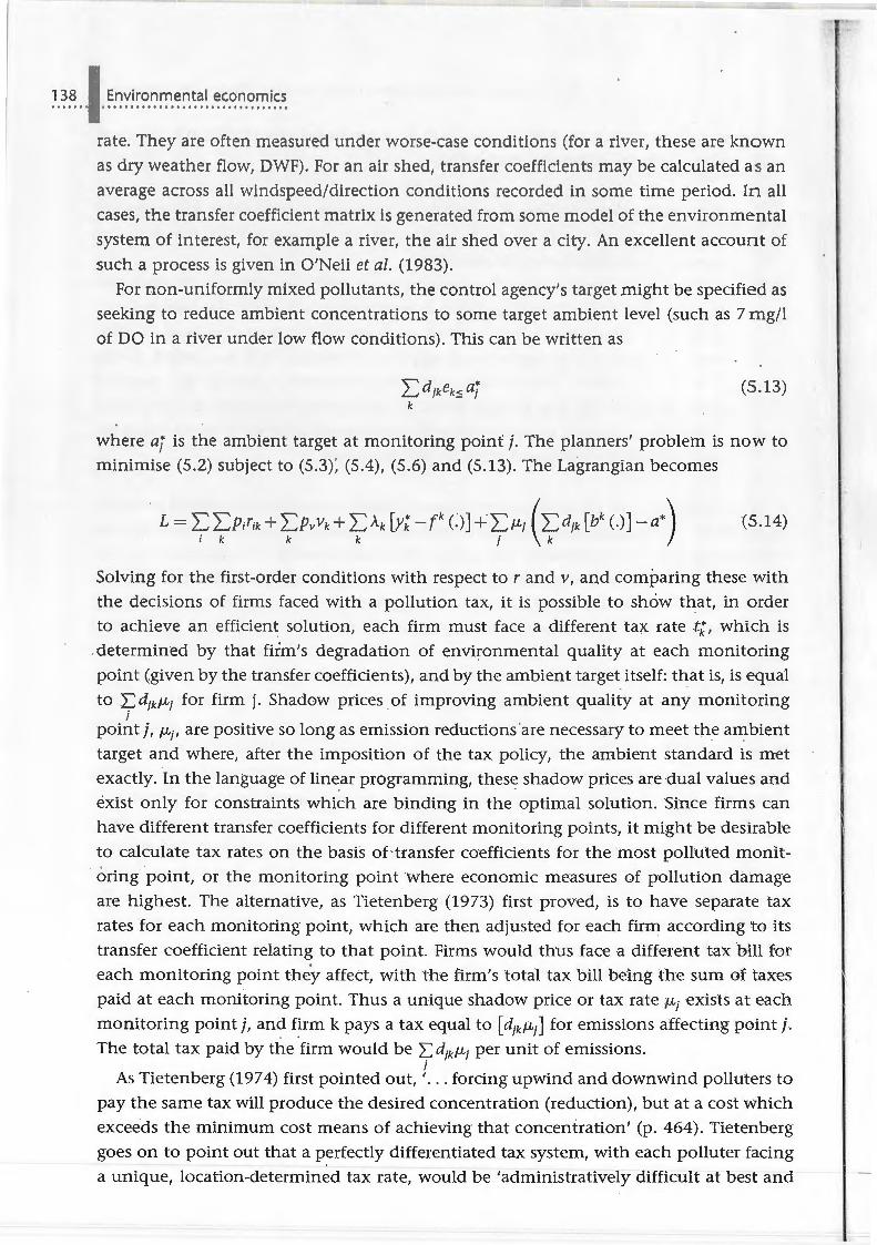
For n on -uniformly mixed pollutants, the control agen cy's targe t might be specifie d as

seeking to reduce ambient concentrations to some target ambient level (such as 7 m g/l

of DO in a river un der low flow conditions) . This can be written as

Ld;kek'!!, aj k

(5.1 3)

where ai is the ambient target at monitoring point j . Th e planners' problem is now to

minimise (5 .2) subject to (5.3); (5.4), (5 .6) and (5.13). The Lagrangian becomes

(5.14)

Solving for the first-order conditions with respect tor and v, and comparing these with

the decisions of firms faced with a pollution tax, it is possible to show that, in order to achieve an efficient solution, each firm must face a different ta:;,c rate tt. , which is

determined by that firm's degradation of environmental quality at each monitoring

point (.given by the transfer coefficients), and by the ambient target itself: that is, is equal

to "E,d;k/L; for firm j. Shadow prices of improving ambient quality at any monitoring i

point j, /L;, are positive so long as emission reductions ·are necessary to meet the ambient

target and where, after the imposition of the tax policy, the ambient standard is met

exactly. In the language of linear programming, these shadow prices are dual values and

exist only for constraints which are binding in the optimal solution. Since firms can

have different transfer coefficients for different monitoring points, it might be desirable

to calculate tax rates on the basis of-transfer coefficients for the most polluted monit­

oring point, or the monitoring point where economic measures of pollution damage

are highest. The alternative, as Tietenberg (1973) first proved, is to have separate tax

rates for each monitoring point, which are then adjusted for ,each firm according to its

transfer coefficient relating to that point. Firms would thus face a different tax bill for

each monitoring point they affect, with the firm's total tax bill being the sum of taxes

paid at each monitoring point. Thus a unique shadow price or tax rate JJ.,; exists at each

monitoring point j, an~ f~rm k pays a tax equal to [ d;k!L; ] for emissions affecting point j.

The total tax paid by the firm would be L d;kµi per unit of emissions. i

As Tietenberg (1974) first pointed out, ' ... forcing upwind and downwind polluters to

pay the same tax will produce the desired concentration (reduction), but at a cost which

exceeds the minimum cost means of achieving that concentration' (p. 464). Tietenberg

goes on to point out that a perfectly differentiated tax system, with each polluter facing

a unique, location-determined tax rate, would be 'administratively difficult at best and

p litica ll y in f as ib l at w r t', so that a tax rat · vary a r z n s but n t within

n thi p int was pr v ided arly on by

'~llution taxes and air quality

mpr mi , su h as a zonal tax yst -m wh r

n s, m i 1 ht be preferred. Empiri al vid n skin °t a l . (1 83), see Box 5.1.

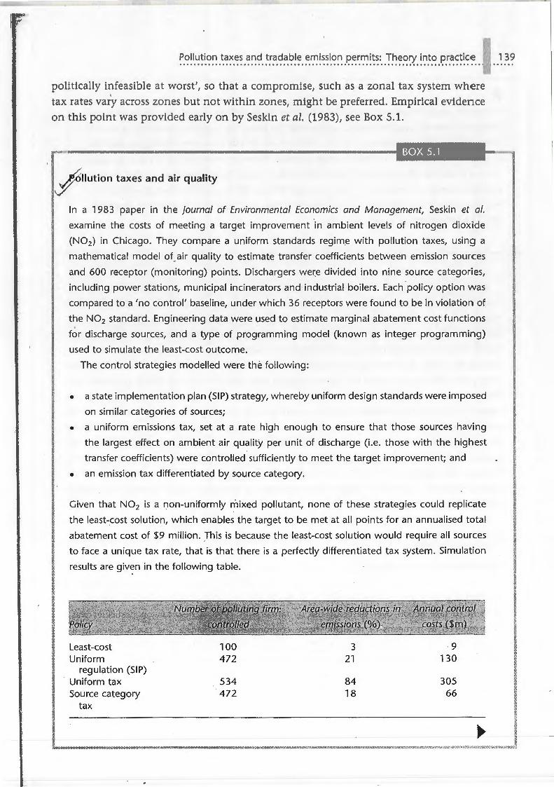
In a 1983 paper in the Journal of Environmental Economics and Management, Seskin et al.

examine the costs of meeting a target improvement in ambient levels of nitrogen dioxide

(N02 ) in Chicago. They compare a uniform standards regim.e with pollution taxes, using a

mathematical model of. air quality to estimate transfer coefficients between emission sources

and 600 receptor (monitoring) points. Dischargers we~e divided into nine source categories,

including power stations, municipal incinerators and industrial boilers. Each policy option w as

compared to a 'no control' baseline, under which 36 receptors were found to be in violation of

the N02 standard. Engineering data were used to estimate marginal abatement cost functions

for discharge sources, and a type of programming model (known as integer programming)

used to simulate the least-cost outcome.

The control strategies modelled were the following:

• a state implementation plan (SIP) strategy, whereby uniform design standards were imposed

on similar categories of sources;

• a uniform emissions tax, set at a rate high enough to ensure that those sources having

the largest effect on ambient air quality per unit of discharge (i.e. those with the highest

transfer coefficients) were controlled sufficiently to meet the target improvement; and

• an emission tax differentiated by source category.

Given that N02 is a non-uniformly mixed pollutant, none of these strategies could replicate

the least-_cost solution, which enables the target to be met at all points for an annualised total

abatement cost of $9 million. This is because the least-cost solution would require all sources

to face a unique tax rate, that is that there is a perfectly differentiated tax system. Simulation

results are given in the following table.

1 9

A m ay b s n, th uni form tax rate has to be set o high (hi h enough to sufficiently restrict

em issions from th m ost dam g ing source) that thi policy has a higher resource cost than the

command and control option of the SIP. The uniform tax rat also gives the biggest reduction

in area emissions, since this high tax rate produces too much abatement from less damaging

sources (note that all poli cies in the table achieve the ambient target level of .air quality). A source

category charge, however, is more efficient than either a SIP or a uniform charge, with tax rates

varying between $15,800 (per year per pound of N02 per hour) for industrial coal-fired boilers

and $13,500 for industrial proc~ss units.

So far in this chapter the discussion has been entirely in terms of a tax on emissions.

However, as noted ·in Chapter 4, the ideas behind an emissions tax can be extended

either to a tax on inputs or to a tax on products. With regard to inputs, Common (1977)

showed that, so long as the 'pollution production function' relating inputs to emissions was known, a desired reduction in emissions could be achieved at least cost with a t ax

on inputs. Input taxes are conceptually very important in the analysis of the control of

non-point pollutants where the monitoring of emissions is either difficult or impossible.

But input taxes could also be utilised for point source emissions, an example being

taxes on the sulphur content of coal as a means of reducing S02 emissions from power

stations. Input taxes may involve problems where an input substitution occurs as a result

of an input tax, and where the substitute input has adverse environmental effects. For

example, taxing CFCs could lead firms to switch to HCFCs, which have been argued to

be more damaging to global climate control, per molecule, than CFCs, as coolants, whilst

taxing particular pesticides might cause farmers to substitute more harmful chemicals (see Box 5.2).

,-P..._e ... st ... i ... c.....,id .... e ....... t-:~x"-"e: ;n ~~~=k.,.,,,_......,.,.-= ... -""'=""""" ........... ,..~..,.-~.,,,,,..._,,,,=="""'""™'""-""'--"""""·· .. ""'-"""""""""''"""""""""""=<>;I

I Worries over pesticide contamination of groundwater resources led the Danish govern-

ment to ·take action over pesticide use by farmers. In 1995, a new tax on pesticides was

introduced as a means ' of reducing these environmental damages. The tax is levied as a

percentage of the wholesale price, 9t rates of 53% (insecticides), 33% (herbicides) and

3% (wood preservatives and rodenticides). Interestingly, these tax differentials do not

I ;~

~ ~ ~

I I ; ij

reflect perceived differences in environmental risk - as economists might recommend - but i ~ I rather the differences in treatment intensity (Schou and Streibig, 1999). The unfortunate · 1

~ implication of this design of tax policy is that ·products which exert higher environmental ;

L .= __ alX'l!::t'~~.a.-M~ .... ..ck'~l$.".3,;;;~=. =---..... ~ ~ 'Xt'~~ ~~::,~~~\%'.:i!t~~,~~~~'.~""""'-,m="""'---=·"'=·==~ ..... r=,1J

damages per kilogram used a re effectiv ly tax d at lower rates th an those th at a re less harm ful,

sine mo re 'environmenta lly friendly' p sticid s tend to sell for higher prices.

Tax revenues, which in 2000 amoun ted to 375 million Danish Krone, are partly (6 0% )

recycled to farmers as subsidies for orga nic fa rming and advice; the remaining 40% is spent on

public research and monitoring programmes. However, it is not thought that the tax is se t a t a

high enough rate to produce real incentive effects, especially given .the nature of th e apply/not

apply decision that farmers need to take during the year (rather than how much to apply) .

This example shows the importance of policy decisions over whether to tax pesticides u sing

a sales tax (the Danish case), or a tax per kilogram of active ingredient, or a tax per unit of

expected environmental damage. This in turn depends on what the exact objective of setting . I

the tax is: to reduce pesticide use, to reduce environmental risks or merely to implement the

polluter pays principle as a means of ra ising tax revenues. Note that the specific aim of the

Danish tax was to raise revenues for pesticide research and extension advice. It is also the case

that a given tax regime may actually encourage farmers to substitute away from currently used

products into more environmentally risky pesticides.

Pesticide taxes now exist in other countries too, including Norway, Sweden, Finland and th e

Netherlands.

Finally, if a stable, predictable relationsh ip between output of a product and emissions

of a pollutant could be found, then a Baumol and Oates tax could be levied on products.

For example, a tax on batteries might reduce cadmium and nickel pollution in drinking

water. However, the relationship between emissions of a pollutant and product prices

may be very difficult to estimate, and are likely to be depend greatly on how and when

that product is both used and disposed of.

5.3 Efficiency properties of tradeable pollution permits

An alternative approach to pollution taxes as a way of achieving a target reduction

in pollution is that of tradeable pollution permits (TPPs). This idea, which originated

with Crocker (1966) and Dales (1968), has gained much popularity recently with envir- .

onmental economists. However, as we _will see, TP.Ps have their own set of problems.

In this section, the basic theory of TPPs is first set out, both for uniformly and non­

uniformly mixed pollutants. Later on in the chapter we review problem areas witq TPPs,

and compare the properties of TPPs and pollution taxes.

From Chapter 3, we know that the major economic explanation for pollution is the

absence of a sufficiently defined and enforced set of private property rights in environ­

mental resources. The main idea behind TPPs is to allocate such rights, and make them

14 ·1

142 nvi ronm n tal nomics

tract abl . Thi r sul t in a market th righ t t p llul · nd consequently in the emergen

fa m arket pri f r this right. Und r rtain nditio ns, this price provides the corre t

in ntiv fo r dis ' harg rs to arrange miss ion I v Is such that a cost-minimising soluti n

is r a h ct. F r a uniformly mixed po llutant, w kn w from Section 5.2 that this involv ·

an quality of MA s across pollut rs. Let u s h w this works out for TPPs, considering

fir t the implest case, namely an assimilative, point-source, uniformly mixed pollutant -

for example, carbon dioxide emissions from power stations. All that the control agen y

is concerned to achieve is a specified reduction in total emissions, irrespective of the

locations of dischargers. Suppose current emissions from a region are 200,000 tonnes

per year, and that the target reduction is 100,000 tonnes, leaving 100,000 tonnes of

continuing emissions. The agency issues 100,000 permits, each one of which allows

the holder to emit one tonne of CO2 per year. Discharges are illegal without sufficient

permits to cover them. These permits may be issued in two ways:

1. by giving them away, perhaps pro rata with existing emissions (this process is

known as 'grandfathering')

2. by auctioning them. We discuss the role of auction design later on.

In either case, firms are then allowed to trade these permits. We expect firms with

relatively high MACs to be buyers, and firms with low MACs to be sellers, assuming the

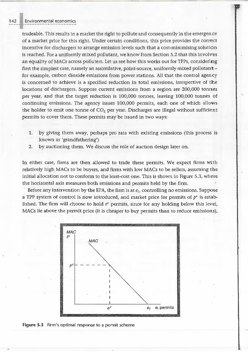
initial allocation not to conform to the least-cost one. This is shown in Figure 5.3, where

the horizontal axis measures both emissions and permits held by the firm.

Before any intervention by the EPA, the firm is at et, controlling no emissions. Suppose

a TPP system of control is now introduced, and market price for permits of p* is estab­lished. The firm will choose to hold e* permits, since for any holding below this level,

MACs lie above the permit price (it is cheaper to buy permits than to reduce emissions),

MAC p

p*

.MAC

e*

Figure 5.3 Firm's optimal response to a permit scheme

e, e, permits

I

but if the firm initially holds m r than e* (and thus can emit t th right of e* ), it

will choose to sell, since the pri it an get (p*) exceeds the mar inal cost of mal<in ·

p rmits available for sale by reducing missions. A firm with higher osts of control Ii n r

pollution will wish to hold mor p rmits given a permit price of p*.

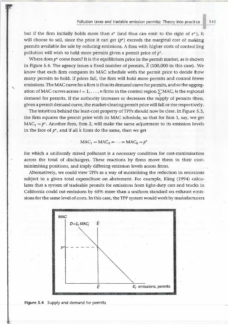
Where does p* come from? It is the equilibrium price in the permit market, as is sh wn

in Figure 5.4. The agency issues a fixed number of permits, E (100,000 in this case). W

know that each firm compares its MAC schedule with the permit price to decide how many permits to hold. If prices fall, the firm will hold more permits and control fewer

emissions. The MAC curve for a firm is thus its demand curve for permits, and so the aggreg­

ation of MAC curves across i = 1, ... , n firms in the control region I: MAC; is the regional i .

demand for permits. If the authority increases or decreases the supply of permits then,

given a permit demand curve, the market~clearing permit price will fall or rise respectively.

· The intuition behind the least-cost property of TP~s should now be clear. In Figure 5.3,

the firm equates the permit price with its MAC schedule, so that for firm 1, say, we get

MAC1 = p*. Another firm,- firm 2, will make the same adjustment to its emission levels

in the face of p*, and if all k firms do the same, then we get

MAC1 = MAC2 = · ·: = MACk =p*

for which a uniformly mixed. pollutant is a necessary condition for cost-minimisation across the total of dischargers. These reactions by firms move them to th.eir cost­

minimising positions, and imply differing emission levels across firms.

Alternatively, we could view TPPs as a .way of maximising the reduction in emissions

subject to a given total expenditure -0n .abatement. For example, Kling (1994) calcu:..

lates that a system of tradeable permits for emissions from light-duty cars and trucks in

California could cut emissions by 65% more than a uniform standard on exhaust emis­

sions for the same level of costs. In this case, the TPP system would work by manufacturers

MAC

D=L; MAC; 'E

· ~

p *1- - - - - -

E E, emissions, permits

figure 5.4 Supply and demand for permits

I

144 nvironm ntal economics

trading mission, permits interna lly (hi h r design emission leve l.s from ome cars against

I w rd sign levels from others) r y trad ing with other car/van manufacturers.

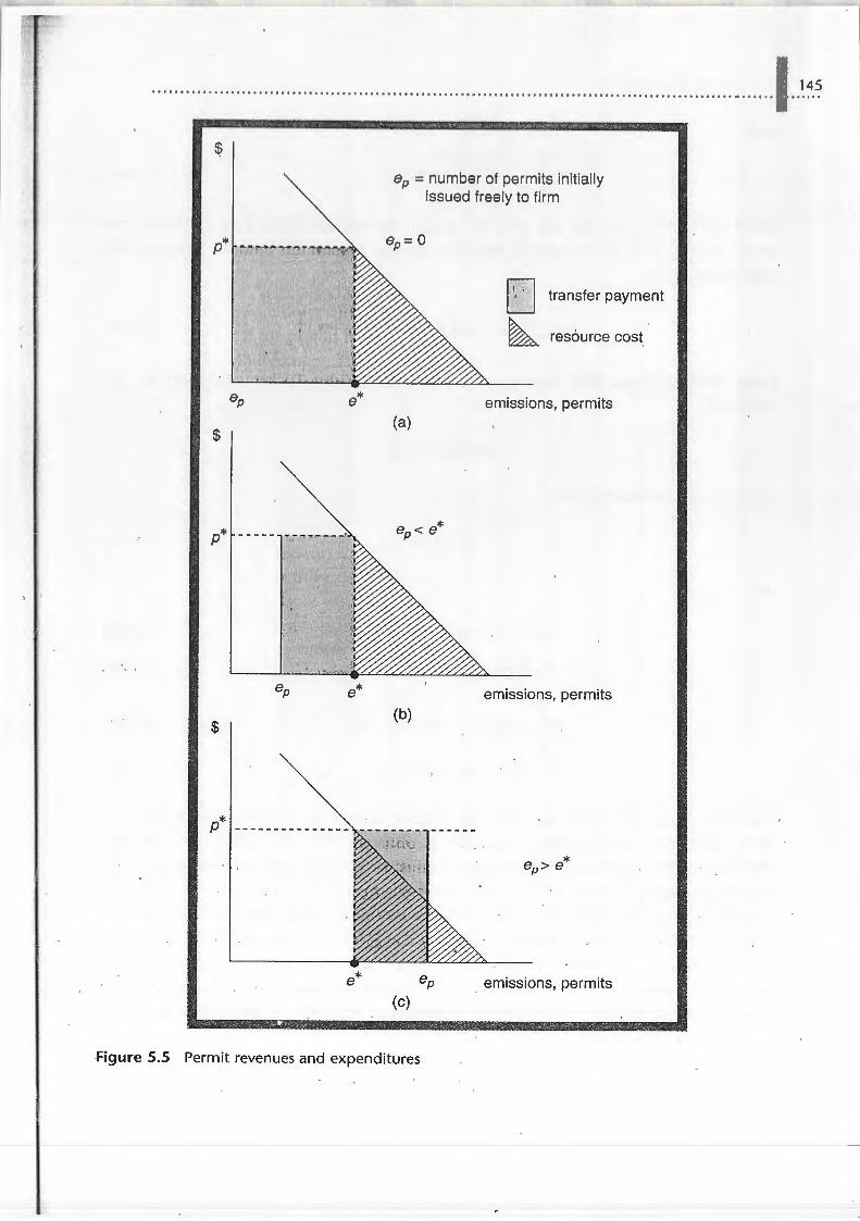
As with the tax scheme, the total financial burden to any individual firm will

c mpos d of resource costs (the sum und r MAC) and transfe r payments. In Figure S. ,

the financial burden for a particular firm is shown under three possible scenarios. In

(a), the firm must pay for all the permits it wishes to hold (say in art auction, wh r

the declared single price is p*, and where the firm has no influence over this price). In

(b), the firm is given some permits, but less than it requires for cost minimisation, so it

buys additional permits from other dischargers. This is equivalent to the firm being on ly

taxed on a fraction of its emissions. In (c), the firm initially receives more permits tqan

it requires, and so sells some. It may be seen that the transfer payments for a given firm

depend on the permit price and whether it is a net buyer or net seller (in all three cases,

resource costs - i.e. control costs - are as shown in Figure 5.5a). For the industry, net

transfers are zero under a 'grandfathering' scheme, since revenue from sales cancels out

permit expenditures in aggregate (although transactions costs will impose an additional

burden on firms - see p. 153). Under ·an auction, however, transfers leave the industry

en bloc. Finally, in the case considered here (a uniformly mixed pollutant), it should

be obvious that permits exchange at a rate of 1:1. If Bloggs sell 100 permits to Smith

and Sons, then Bloggs must cut their emissions by 100 units, and Smith may increase

theirs by 100. This is because control, as has already been said, is aimed at the total

of emissions, not their spatial location. This will clearly not hold when we consider

non-uniformly mixed pollutants.

Let us now establish our main results so far considered more formally. The original

proof of the least-cost property of TPPs is due to Montgomery (1972), but our proof draws

on Tietenberg (1984). Suppose that A represents the level of carbon dioxide (a uniformly

mixed pollutant) emitted from the control region, and is given by:

(5.15)

where a is emissions from other sources including natural sources, er are 'uncontrolled'

emissions from i = l, ... , n polluting firms (as point er in Figure 5.3) and xi are reductions

in emissions. Finns face control costs Ci which depend solely on its level of emission

reduction:

Ci= Ci (xJ (5.16)

where Ci(xJ is a twice-differentiable function, with C' > 0 and C" > 0 (with C' and C"

representing first- and second-order derivatives of C). The control agency wishes to hold

total emissions at or below some level A, which is assumed to be less than the current

total of discharges. The agency's problem is thus to achieve

Min Lei (xi) (x;)

(5.17)

• • • • • • • • 0 • 0 • • • • • • • • • • • • • • • " " 0 • "• • • 0 0 • • • • • • • • '• • • • • • • • • • '• • • • • • • ••••••I IO O O • • o • • o •, , • • •, o o, • •, •, o • 0 • • • o, o - , , , , , ,

$

$

p*

* e

* e

eP = number of permits initially issued freely to firm

(a)

(b)

(c)

D transfer payment

~ resource cost

emissions, permits

emissions, permits

emissions, permits

Figure 5.5 Permit revenues and expenditures

145

146 nta l economi

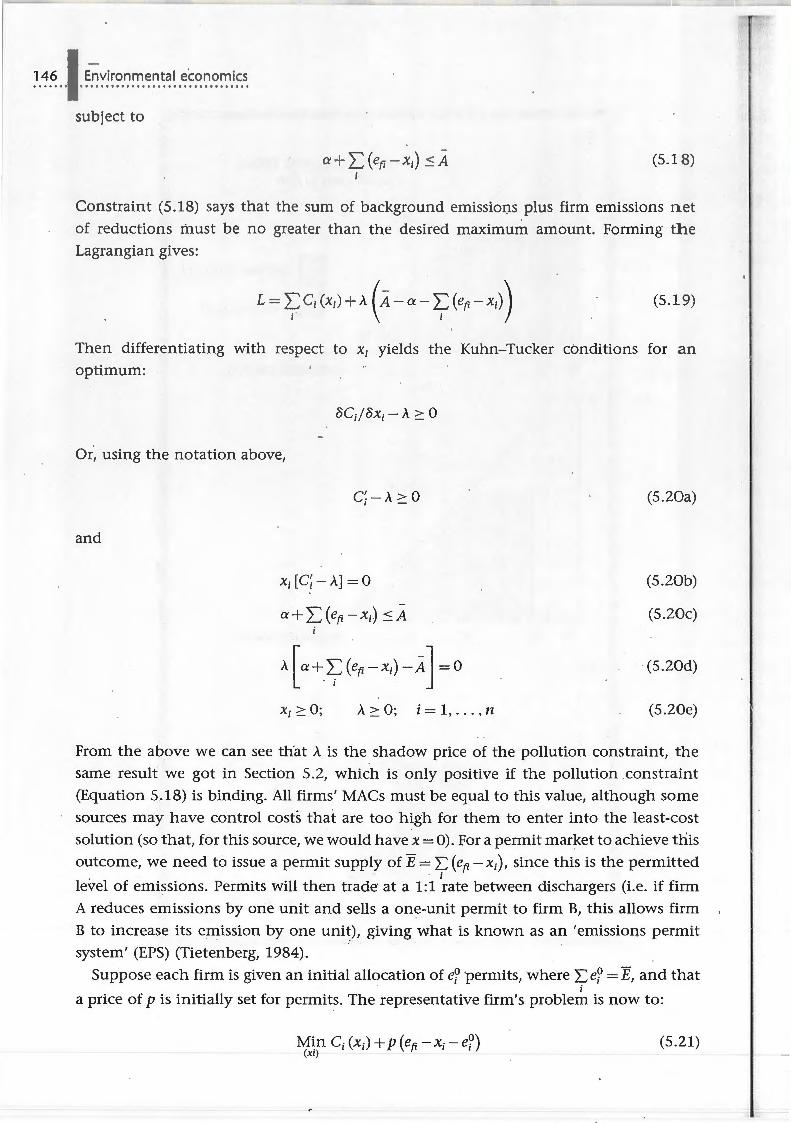
sub ject to

(5.1 8)

Constraint (5.18) says that th um of background emissions plus firm emissions n t

of reductions must be no grea ter than the desired maximum amount. Forming th Lagrangian gives:

(5.1 9)

Then differentiating with respect to xi yields the Kuhn-Tucker conditions for an optimum:

oC. /ox -- A > o I I -

Or, using the notation above,

C'. - A>O I -

(5.20a)

and

xi[C;-A]=O (5.20b)

a + L(efi-xi) :::A (5.20c)

{,+~(er-x;)-A J =0 (5.20d)

xi=:': O; A::':0; i = 1, . .. , n (5.20e)

From the above we can see that A is the shadow price of the pollution constraint, the

same result we got in Section 5.2, which is only positive if the pollution constraint

(Equation 5.18) is binding. All firms' MACs must be equal to this value, although some

sources may have control costs that are too high for them to enter into the least-cost

solution (so that, for this source, we would have x = 0). For a permit market to achieve this

outcome, we need to issue a permit supply of E = L (efi -xi), since this is the permitted . i

level of emissions. Permits will then trade at a 1:1 rate between dischargers (i.e. if firm

A reduces emissions by one unit and sells a one-unit permit to firm B, this allows firm

B to increase its emission by one unit), giving what is known as an 'emissions permit

system' (EPS) (Tietenberg, 1984).

Suppose .each firm is given an initial allocation of e? permits, where I:: e? = E, and that i

a price of p is initially set for permits. The representative firm's problem is now to:

(5.21)

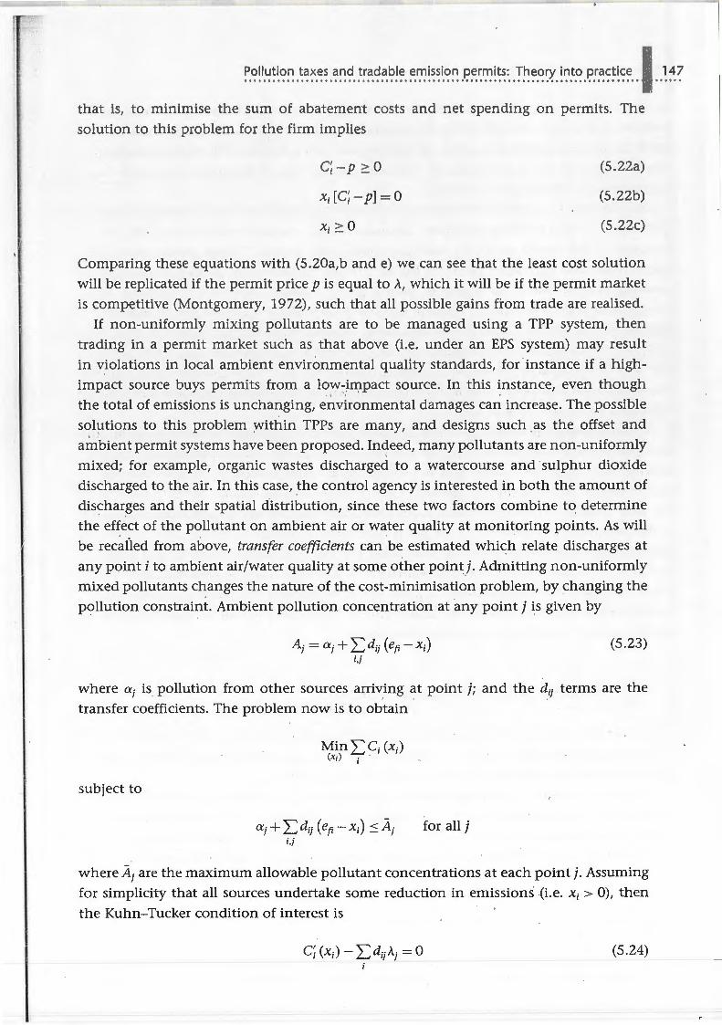
that is, t minim is th sum f a ba t m nt sts and n · t spending on permits. Th

s luti n t thi · pr l n f r th firm implies

;- p ~o x;[C; - p] = 0

X; ~ Q

(5.22a)

(5.22b)

(5.22c)

Comparing these equations with (S.20a,b and e) we can see that the least cost solution

will be replicated if the permit price p is equal to A, which it will be if the permit market

is competitive (Montgomery, 1972), such that all possible gains from trade are realised.

If non-uniformly mixing pollutants are to be managed using a TPP system, then

trading in a permit market such as that above (i.e. under an EPS system) may result

in violations in local ambient environmental quality standards, for instance if a high­

impact source buys permits from a low~.impact source. In this instance, even though

the total of emissions is unchanging, environmental damages can increase. The possible

solutions to this problem within TPPs are many, and designs such . as the offset and ambient permit systems have been proposed. Indeed, many pollutants are non-uniformly

mixed; for example, organic wastes discharged to a watercourse and sulphur dioxide

discharged to the air. In this case, .the control agency is interested in both the amount of

discharges and their spatial distribution, since these two factors combine to determine

the effect of the pollutant on ambient air or water quality at monitoring points. As will

be recailed from above, transfer coeffi.cients can be estimated which relate discharges at

any point i to ambient air/water quality at some other point}- Admitting non-uniformly

mixed pollutants changes the nature of the cost-minimisation problem, by changing the

pollution constraint. Ambient pollution concentration at any point j is given by

Ai= ai + L_d;i (efi -x;) i,i

(5.23)

where ai is pollution from other sources arrh7,ing at point j; and the d;i terms are the

transfer coefficients. The problem now is to obtain

subject to

Min"I:,C;(x;) (x;) i

ai + L_d;i (efi -x;) ::S Ai i,i

for all j

where Ai are the maximum allowable pollutant concentrations at each point j. Assuming

for simplicity that all sources undertake some reduction in emissions {i.e. X; > 0), then

the Kuhn-Tucker condition of interest is

(5.24)

147

that a h s is qual to the weigh t d av ra f the shadow cost of

miss i ns rcdu ti ns n d d to hi t the targets. Put an th r way, there is now a shadow

pri (A;) at ea h m nit rin p in t, so tha t we h ave g t away from the simple 'equalise

MA ' rule t h at was r .J va1 t in the uniform, mixing a . This system of permits is

known as an ambient perm it sys tem.

One design issue with permit m arkets, for either uni fo rm·ly or non-uniformly mixed

pollutants, is whether fi rms should be allowed to 'bank' emiss ion reduction credits. For

instance, a firm could decide to abate more than was required in the present period,

earn credits and then bank these for use in a future period , when perhaps it thought

abatem ent costs would be high er or permit prices high er. Allowing the banking of

permits has been argued to be desirable since it can even out spikes in permit markets

due to, say, sudden increases in the demand for electricity - as happened in California

in 2000, which produced big increases in NOx permit p rices (Ellerman et al. 2003), can

act as a hedge against uncertainty; and cari encourage early reductions in emissions.

However, regulators may worry that hanking will result in violations in environmental , ' '

standards in some time periods.

A second design issue relates to the possibility of allowing trade between point and

non-point sources of pollution. For instance, both point sources (such as industrial plants

and sewage treatment works) and non-point agricultural run-off are responsible for

severe oxygen depletion in the northern Gulf of Mexico (Ribaudo et al. 2005). Allowing

for trade between these two source types allows for cost-savings in pollution control,

since marginal abatement costs for point sources were found to be typically greater

than marginal abatement costs for non-point sources. Simulations showed that a net

welfare gain of $46 billion was possible with such tradin'g; although, interestingly, the

modellers made the assumption of a 1:i rate of trading between the (expected) reduction

in agricultural-source pollution and each unit of reduction avoided for point sources

within each of 21 districts included in the model.

y.: _'. . -~~-~~~~-~~- ~i-~~- ?.~~1-~~-i~~ -~~-~~~ ................................. . In Section 5.2, problems facing a regulator when a non-uniformly mixed pollutant is

the environmental concern were noted. We now list some further problems with tax

policies for the achievement of pollution reduction targets.

First, the pollution control agency must set the tax rate (or vector of rates for a non­

uniformly mixed pollutant) at the appropriate level(s) to achieve the desired improve­

ment in environmental quality. To get this exactly correct requires full information on

abatement costs and transfer coefficients. As Baumol and Oates originally argued, agen­

cies could iterate onto the correct tax rate (for a uniformly mixed pollutant) by setting a

best-guess rate and then observing the consequent reduction in emissions. If this was too

great, the tax rate should be reduced; if too little, then the tax rate should be increased.

However, this neglects three problems: (}') setting an initially incorrect tax rate can lock

firms into incorrect investments in pollution control equipment, preventing them from

minimising costs (Walker and Storey, 1977); (2) setting an initial rate too low may result i'

in irr v rsib l , r r v rsibl buts ri us, dama t th nviron ment and (~ h aggr gat

MA fun li n is I t stab l th r u h tin . It will b ch anging in r al terms owing t

fluctuation's in en rgy ost ·, input st and pr du t prices, and also in nominal t rms

as the r sui t f infla tion. ett ing th tax rat rr t may thus be a very tricky task.

A secon d p r bl m con em the issue f n w entra nts to a region. Suppose the m ajor

pollution pr b l m in an es tuary is emi ssions from oil refining . If new refineries are

establish ed in th area, then th e aggregat MAC fun ction will shift to the right, implying

that, unless the tax rate is increased, aggregate emissions will increase. This is really just

another aspect of the information problem discussed in the preceding paragraph.

A th_ird issue relates to the case of pollution problems where the undesirable environ­

mental effec t is brought about by a number of pollutants. The problem for the environ­

mental regulato r is then to set the correct taxes across this 'basket' of pollutants to achieve

the environmental target. Perhaps the best exampl_e is global warming, which is caused

by a number of gases, carbon dioxide (CO2 ) , methane (CH4 ), nitrous oxide (N2 0) and chlorofluorocarbons (CFC11 and CFC12). The increased accumulation of these gases is,

according to many global models, producing an increase in global mean temperature. A

comprehensive account of economic analysis of the greenhouse effect is provided in Owen

and Hanley (2004). Michaelis (1992) considers this problem from the point of view of how

to design a comprehensive GHG tax system. The important question here is the level of

efficient relative tax rates for the four main GHGs. Michaelis also considers the dynamics of

this problem, in that there is not only a finite assimilative capacity in each time period for

GHGs, but also a constraint on the total stock if undesirable warming is to be avoided. Each

pollutant has a different contribution to global warming potential. The solutiop to this

control problem implies that higher tax rates will be imposed on GHGs with higher a and

lower 'TJ values, where a represents the relative warming potential of each gas, and where 'TJ

represents the natural degradation rate of each gas in the atmosphere. Furthermore, for a

given GHG the optimal tax rate evolves overtime at a rate of (1 +r/1- TJ), where r is the rate

of discount. Michaelis shows that absolute tax rates depend on the initial stock of GHGs,

the time period over which the problem is considered, the absolute level of abatement

costs and the initial period level of emissions.

Pollution taxes can be objected to on equity grounds. Pollution taxes might

have undesirable re-distributive effects oh households: for instan~e, a tax on energy

consumption by households aimed at cutting CO2 emissions might well hit poorer

households harder than richer households, since the former tend to spend a higher

proportion of their income on energy than the latter.. -For instance, the Danish CO2

tax has been found to impose proportioi:iately higher costs on poorer households in

Denmark than on ,richer households (Wier et al. 2005). Box 5.3 gives more evidence on

this issue. Firms could also raise objections to the equitability of taxes. Pezzey (1988) has

argued that pollution taxes can over-penalise firms in terms of what is conventionally

understood about the polluter pays principle (PPP). In Figure 5.6, a single polluter on

a river .is shown, in terms of the MAC schedule, and a marginal damage cost (MDC)

schedule, which relates the amount of emissions to the monetary value of environmental

damages caused by these emissions.

149

150

Distributional effects of economic instruments

Environmental taxes send signals to consumers by making consumption of environmental

resources more expensive. However, there are conce rns that their effect could be 'regressive', by

hitting lower income households disproportionately. Resea rch by Dresner and Ekins (2004a,b)

investigated the possible impact on low-income households in four areas: domestic use of

energy, water and transport, and domestic generation of waste. It also considered whether any >

negative impacts could be reduced if the tax or charge were designed appropriately, or if a

compensation scheme were introduced. The study found the following :

• Low-income households' use of energy, water and waste disposal services and their use of

cars where they own them, is disproportionate in relation to their income. This confirms

that a flat-rate tax or charge applied to such usage would be regressive.

• For the average low-income household, the disproportionate impact could be removed

through an·appropriate (i .e. non-flat rate) design of the tax or charge scheme and/or by intro­

ducing a compensation scheme along with the tax or charge-although this would clearly have

trans.actions costs associated with it, and could produce knock-on incentive effects.

• However, use of environmental resources tends to vary widely within a given income group.

This means that, in practice, some low-income households would end up as net losers

from any charging-plus-compensation scheme, even when the scheme leaves low-income

households better off Qn average.

• It may be possible (e:g . with water use) to relieve this re-distributional burden through

further special arrangements. Alternatively, it may be necessary to tackle the underlying

cause of the hardship (such as energy-inefficient buildings) if pricing is to be used as an

instrument of policy.

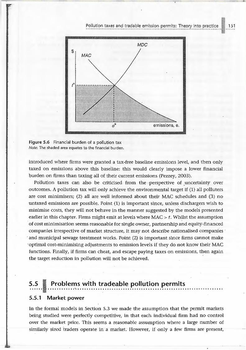
If MDC were known, then an ( optimal) tax of t * could be set, realising emissions of e*

if the firm is a cost minimiser which is fully informed as to its MAC schedule .. However,

the totaJ financial burden to the firm (the shaded area, being the sum of abatement costs

and tax payments) exceeds what P·ezzey calls the conventional PPP and the 'extended

PPP'. The conventional PPP is interpreted as meaning that firms should pay their own

control costs up to the socially desired level of control e* . The extended PPP adds to this

burden the value of damages done by this socially desired level of emissions, the area

under MDC up to e* . That the financial burden to the firm under the tax of t * exceeds

both these amounts might be judged to be unfair. The size of transfer payments implied

by a pollution tax policy has been argued to have been a major barrier to the acceptance

of pollution taxes. in the OECD. However, in principle this obstacle is surmountable at

the aggregate level, since transfers could be returned to industry as lump sum payments

(e.g. as capital grants for investment in pollution control). A tax system could also be

1 I

* e

Figure 5.6 Financial burden of a pollution tax Note: The shaded area equates to the financial burden.

MDC

emissions, e.

introduced where firms were granted a tax-free baseline emissions level, and then only

taxed on emissions above this baseline: this would clearly impose a lower financial

burden on firms than taxing all of their current emissions (Pezzey, 2003).

Pollution taxes can also be criticised from the perspective of .uncertainty over

outcomes. A pollution tax will only achieve the environmental target if (1) all polluters

are cost minimisers; (2) all are well informed about their MAC schedules and (3) no

untaxed emissions are possible. Point (1) is important since, unless dischargers wish to

minimise costs, they will not behave in the manner suggested by the models presented

earlier in this chapter. Firms might emit at levels where MAC> t. Whilst the assumption

of cost minimisation seems reasonable for single owner, partnership and equity-financed

companies irrespective of market structure, it may not describe nationalised companies ·

· and municipal sewage treatment works. Point (2) is important since firms cannot make

·optimal cost-minimising adjustments to emission levels if they do not know their MAC

functions. Finally, if firms can cheat, and escape paying taxes on emissions, then again

the target reduction in pollution will not be achieved.

5.5 Problems with tradeable pollution permits ...... · ..... ............ · ................................................................ . 5.5.1 Market power

In the formal models in Section 5.3 we made the assumption that the permit markets

being studied were perfectly competitive, in that each individual firm had no control

over the market price. This seems a reasonable assumption where a large number of

similarly sized traders operate in a market. However, if only a few firms are present,

151

2

f th s firms is large enough to influ n

buyin an I · ll in havi ur, th n the l ast- os l pr

th p rmit price through its wn

p rty f TPPs may not h Jd, and

th a gr -gat sts f th p rmit s h em an in r as .

Why hould a firm s k to influence th p rmit pri ? Two possible motivation are

1. to minimis it costs of compliance; and

2. to disadvantag its rivals in the product market.

Consider a firm which holds a relatively large stock of permits. This firm can earn

revenues by selling permits; the costs it incurs in free'ing-up permits for sale are given

by its MAC. Clearly, the firm would like to receive as high a price for each permit as it

can; if it has monopoly market power, then by restricting the number of permits sold

on the market it can push up the price (Godby, 2000). This results in a welfare loss, with pollution by the dominant firm being too high, and pollution from the competitive

fringe being too low. The extent to which a firm will choose to engage in such behaviour

clearly depends on the price elasticity of demand for permits and the slope of the firm's

MAC schedule, since the latter determines the price of freeing up permits for sale, whilst

the former (which in turn depends on other firms' MAC schedules) dictates the degree

to which the permit price will rise as the number of permits offered for sale decreases

(Hahn, 1984; Misiolek and Elder, 1989). Alternatively, with monopsonistic power in the

market, by buying fewer permits the firm can reduce the price it must pay for those

permits it does purchase. Again, the cost of this price-setting behaviour is given by the

firm's MAC schedule,. the· slope of which will influence the degree to which the firm

engages in such behaviour. Summarising the above, we may say that in the monopoly

case the market power firm spends too little on abatement, as it sells fewer permits than

it would do in the competitive outcome, to keep permit prices high. Other firms spend

too much on abatement. In the monopsony case, the market power firm spends too

much on abatement and buys too few permits relative to the competitive case, to keep

permit prices low. Hahn (1984) found that the initial allocation of permits affected both

the post-trading outcome and the permit price, unlike the 'neutrality of initial allocation'

result in a competitive market. However, Cason et al. (2003) argue that the extent to

which market power affects the least-cost outcome depends also on how trading occurs:

in their study, a continuous_ double auction (where buyers and sellers post sell/buy prices

publicly, and can accept each others' offer at any time) resulted in only minor losses in

market efficiency due to monopoly or duopoly, relative to the competitive . equilibrium.

There is little empirical evidence from actual permit markets of the effects of price­

setting behaviour. Godby (2000) and Stavins (1998) report no evid~nce of 'market power

affecting outcomes in the US sulphur market, whilst the UK National Audit Office note

that this was not a problem in the UK carbon trading scheme, since institutional rules

prevented any one firm from holding more that 20% of all permits. Many studies have

however pointed out the potential for such urn;:ompetitive outcomes to emerge. OECD

(2000) estimate that Russia and other former Soviet Union countries will command a

large share of permits for sale under international carbon trading due to their 2005

missi ns being well below th ir J 9 0 I v ls: this mark t pow r is stimated to r du

potential gains from tract und r a :ur p an carbon trading h m by 20%. Al th

national scale, Crampton and K rr's (1999) simulation of a US 2 market predi. t d .

that no one firm would control m r than 6% of the market. At a more local a l ,

Eheart et al. (1980) found that only tw sources would control 80 per cent of all permits

sold for phosphorus discharges into La k Michigan.

Maloney and Yandle (1984) modelled price-setting behaviour through the establi h­

ment of cartels. For monopoly power, the increases in total ·control costs over the

competitive base line were at most 41 per cent (with 90 per cent of the sources own ed by

the monopolist); for monopsony power, the greatest increase in total abatement costs

was only 8 per cent, again at a 90 per cent holding for the monopsonist. However, v n

in the worst monopoly case, the (uncompetitive) permit market still achieved a 6 6 per

cent saving over the command-and-control outcome. Hahn (1984) considers a p rmit I • • •

market for particulate sulphates in the Los Angeles region, a market in which earlier

work by the author had shown that one source (a power station) could be responsible for

over 50 per cent of controllable emissions. _In this case, the market clearing permit price

varies.from $3200/ton .with monopsony, to the competitive price of $3900, to a price of $2~ 1000/ton with Jull monopoly power. Cason et al. (2003) use experimental e'conomics

methods to simulate the effe,cts on prices, trading and efficiency of both monopoly and

duopoly in an emissions tr~ding scheme for nitrogen pollution permits in Port Phillip

Bay, Victoria, Australia. As noted above, a double-auction design is used, along with

actual marginal abatement cost functions estimated for P.Olluters in the Bay. The authors

find rather small effects on cost-efficiency from monopoly or duopoly, and little jmpacts

from changing the initial allocation of permits across sources - a rather encouraging

finding for the development of TPP approaches to real-life pollution control problems

where large firms dominate waterbodies, and/or where few traders are involved.

Moving onto the second of the two motivations set out above, Misiolek and Elder

(1989) analyse the case where firms seek to raise the permit price so as to make .entry

to a product market less attractive for potential rivals. This may occur when actual or

potential rivals must purchase permits in the same market as that of the fin:n wishing

to take . exclusionary action. Misiolek and Elder argue that such exclusionary action is

most likely to be taken by large firms with relatively low . MA Cs, to exclude smaller

potential or ,actual entrants with higher MA Cs. They show that exclusionary action can

increase both short-run and long-run profits for a firm. In a sense, exclusionary behavi.our

counteracts cost-minimising manipulation: we have seen above that the latter can lead

to a firm with monopsony power buying too few permits; yet exclusionary behaviour

will cause it to wish to buy too many permits. For a monopolist, however, whose cost­

minimising manipulation involves selling fewer permits than in the competitive case,

the effect of exclusionary manipulation is to worsen the distortion. As an interesting

twist on this story, Carlen (2003) speculates that, in international permit trading of

carbon dioxide, national governments could put pressures on firms not to trade permits

with foreign competitors in the same industry, in order to protect the domestic industry

from international competition.

154

I

nvir nm ntal economics

5.5.2 Transactions costs

Tran action costs are the costs of trading: of finding someone to trade with, of negoti­

ating and concluding this deal and then of clearing the deal (if needed) with the regu­

lat r. High transactions costs can form a barrier to permit trading, and thus prevent al

possible cost savings from being realised (Stavins, 1995). Transactions cost can determin

whether the initial allocation of permits across sources matters. Also of importance is

whether transactions costs are increasing or decreasing with the volume of trade: fo I

example, they could fall as the volume of trade rises due to learning-by-doing effect:s

(Cason and Gangadharan; 2003). Uncertainty as to whether trades will be approved by

regulators, for instance where trading rules are in place to handle non-uniform mixing

problems, is also important in deciding the effects of transa<;:tions costs on the efficiency

of a TPP system (Montero, 1997).

How serious is the problem of transactions costs in reality? Tietenberg (1990) ha s

argued that the relatively small cost-savings achieved by a variety of permit trading

schemes operating for air pollution in the USA prior to 1990, such as the 1977 offsetting

scheme and the 1979 'bubble' scheme, was due to high transactions costs. High transac­

tions costs have also been put forward as the main reason why the Fox River scheme in ' ' '

Wisconsin failed to realise any trades at all after it was introduced in the 1980s, despite ' ' .

prior simulation work which showed that very significant potential cost savings existed

(O'Neil et al., 1983). One practical solution to reducing transactions costs as a barrier to

cost-minimisation is for the regulator to run an electronic 'bulletin board' service, where

offers to trade are posted in terms of prices and quantities of permits: this is likely to be

a feature of the new EU Emissions Trading System, which is described in Box 5.4.

The European Union's Emission Trading Scheme

As part of its programme of measures to achieve its Kyoto targets on reducing GHG emis­

sions (see Chapter 6), the European Union introduced an Emissions Trading Scheme (ETS) for

carbon dioxide·with effect from January 2005. Those covered by the scheme will include the

largest point source emitters of carbon dioxide, including electricity generators, oil refineries

and the iron and steel industry. Some 12,000 'installations' are covered by the scheme. Indi­

vidual member states published National Allocation Plans in 2004, which set out the initial

allocations of permits to affected firms/sectors: these National Plans were then vetted by the

European Commission. Interestingly, the ETS scheme came about partly because of severe

political pressure from member states against a putative carbon tax being proposed by the

European Commission.

The ETS scheme is a cap-and-trade scheme, in that, under the National Allocation Plan,

each sector/firm is given a number of emission permits equal to its allowance or cap, for each

I I fl t

I rt

., LAC:1.~~~~~'!:=~~~~~~..:r.R1:~~~~=•.,"m·ar•==-====•=---=:!!

period over which the sch m operates . In the first phase (2005- 2007), these allowanc ar

mainly being issued free, with 5% being retained for auction. Firms that cut emissions below

their individual cap can then either sell the freed-up permits, or bank them for thei r own

future _use (although not all m ember states may allow banking). Similarly, firms who fail to

redu.~e emissions to their cap can cover the difference by buying permits, either from emission

reductions within the EU, or from emission reductions outside the EU which are sanct ioned

under the Flexible Mechanisms of the Kyoto protocol. A second phase of the scheme runs from

2008-2012.

Much criticism has been levelled at the ETS. For example, Vertedal and Svendson (2004) have

criticised the implications for competitiveness and rent-seeking behaviour in the EU given the

grandfathering method of allocation, whilst Boemare and Quirion (2002) note that problems

may exist due to national non-compliance on the part of member states. For an excellent

overview of the scheme, including the c_hal_lenges it faces and comparisons with US schemes,

see Kruger and Pizer (2004).

155

- ....... .._ ...... _....., __ """"" ________ = ....... ----·------...... -"""""''"""'''""""""". ,..... ___ _

5.5.3 Trading rules and non-uniform mixing

In Section 5.3, two designs of permit system were mentioned: an emissions permit system . . . (EPS) and the ambient permits system (APS). Under the forme"r, permits are denominated

in units of pollutant emitted (one permit permits one tonne of BOD, for example). Trades

of permits between firms take place at a one-for-one rate. In other words, if source A

sells one permit, it must reduce its emissions by the amount of emission covered by the permit. When source B buys this permit, it can increase its emissions by the same

amount. Total emissions therefore do not increase. The EPS is a simple system, and for

a uniformly mixed pollutant it may work well. For non~uniformly mixed pollutants,

however, trades under an EPS could result in violations of ambient quality targets, since if

source B is located in a more sensitive part of, say, a river, then its i_ncrease of x tonnes of

emissions will do more damage than is avoided by A reducing its emissions by x tonne_s.

To get around this problem, the APS was proposed. However, this has the problem

that it is a very complicated market. Permits are denominated in units of damage at

receptors. There is a separate market "in permits at each receptor, and firms must trade

in as many markets as their emissions affect receptors. For a pollutant such as sulphur

dioxide, this could be a very large number of markets. Transaction costs would therefore

be relatively high, whilst the number of traders in each market would be relatively low,

giving rise to potential problems of imperfect competition (see above). What is more,

total emissions can rise as a result of trading, which may cause knock-on environmental

problems. If firm A sells permits which permit a reduction of 1 mg/1 in dissolved oxygen

at receptor point z, and if B's emissions have a relatively small impact on dissolved

156 nvironmental econom ics

xyg n at point z, then B can in

st savings under the APS ar t

wa ter quality down to the targ t l

r as .it emissions by more than A reduces its own.

n xt nt realised by allowing a d gradation of air or

v l at receptors where, pre-trad , air/water quality i

better than the target. An APS may also result in an increase in th long-range transport

of pollutants (Atkinson and Tietenberg, 1987).

A variety of other trading rules have been proposed. All basica lly work on the prin­

ciple of permits being denominated in units of emissions (one permit per tonne of

BOD), but with rules governing trades in permits to stop the violation of ambient

quality targets. The three best known of these trading rules systems are the pollution

offset, the non-degradation offset and the modified pollution offset. The pollution offset

system (Krupnick et al., 1983) works by imposing a rule on trades that they may not

violate the ambient quality target at any receptor point. However, this is consistent with

worsening ambient quality up to the target level and an increase in total emissions. The

non-degra.dation offset imposes the additional constraint that total emissions may not

increase as a result of trades (Atkinson and Tietenberg, 1982). Finally, the mo<;lified offset

(McGartland and Oates, 1985) allows trades so long as neither the pre-trade quality level

nor the target level, whichever is the stricter (cleanest), is not violated. As Atkinson and

Tietenberg (1987) point out, there is no general conclusion which can be drawn as to

the relative cost-effectiveness of the modified and non-degradation offset systems (they

rule out the simple offset system as being incompatible with environmental quality

objectives). Comparisons must instead be rnade on a case-by-case basis. lntheir empirical

analysis, they find the following for models of two US cities (St Louis and Cleveland) for

the control of sulpl)ur oxides (Cleveland) and particulate emissions (St Louis). In each

case, ·the two offset systems are compared with the theoretically obtainable least-cost

solution (which in th,is case would result from a perfect implementation of an APS) and

with the command-and-c~ntrol alternative of uniform design standards (denoted SIP,

for state iJ,nplementation plan). (SIPs were prepared by all US states in response to the

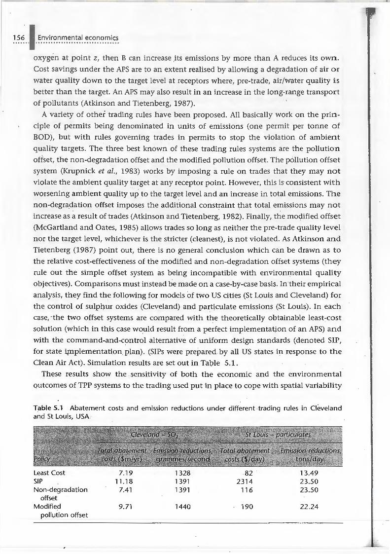
Clean Air Act). Simulation results are set out in Table 5.1.

These results show the sensitivity of both the economic and the environmental

outcomes of TPP systems to the trading used put in place to cope with spatial variability

Table 5.1 Abatement costs and emission reductions under different trading rules in Cleveland and St Louis, USA

Least Cost 7.19 1328 82 . 13.49 SIP 11.18 1391 2314 23.50 Non-degradation 7.41 1391 116 23.50

offset Modified 9.71 1440 190 22.24

pollution offset

•,

in envir nm nta l im pa t ·. N t , h w v r, that b th Tl P sy t ms are cheaper than r u­

la tion, r p r s n t d y th IP u t m .

It is w rth m nti nin that ven wh r th damag s d n by emissions are depe nt

on th ir patial I ati n, TI I h m s may ch s t ignor this fact, and opt f r a

simpl r EPS d sign. F ·r in tan , th is is what has happ n d under the Acid Rain trading

programm in the U (see Box 5.5).

Sulphur trading in the USA

In 1 990, the US Con'gress passed Clean Air Act Amendments which introduced a TPP system

for the control of su lphur dioxide emissions from large point sources (primarily power stations) .

Stavins (1 998) gives an excellent analysis of the political economy factors underlying the

introduction of the scheme. The impetus for this measure came from Bush's campaign promises

to take action on acid rain, and from support for the idea of TPPs to .achieve this from the

Environmental Defence Fund and members of the President's Council of Economic Advisors.

Rising pollution control costs in the US gave a further impetus to the use ?f an economic

instrument, rather than more regulation. What is more, great variations were known to exist

in MACs across sources, implying large potential cost savings to be made from trading. Finally,

there was no existing system for controlling acid rain causing emissions, so no status quo bias

was present in the minds of regulators.

. The system was intended to bring about a 10 million ton (50%) reduction in emissions of

S02 from large stationary sources relative to 1980 levels. Most permits were 'grandfathered'

(a great deal of time was spent in arguments over this allocation, both across regions and

industry groups), although a s~all proportion were retained by the EPA for allocation to new

sources, and for auction at the Chicago Board of Trade. As Joskow and Schmalensee (1998)

point out, the decision to go with grandfathering rather than auctions is partly explainable by

the greater control this gave politicians and administrators over the geographic distribution

of financial burdens to firms . Compliance with the scheme is encouraged by a penalty of

$2000/ton for unauthorised emissions.

Sulphur permits are denominated jn annual tons of emissions, and can be banked. Permit

prices fell from $131 to $95/ton during the first five years of trading (Ellerman et al., 1999).

157

I I While many trades ~ave occurred, most have been internal rather than external, and high

::":::;~:::::::::~:~:::: e:~~e::~;:~~~:::~::~f }~t::s:::~:i3:::~~:::7:::;:::~ I billion per year, and by Ellerman et al. as between 1 /3 and 1 /2 of the cost without trading . ~

I ~

~ This cost saving is partly due to the phenomenon whereby the existence of trading possibilities I I h_as reduced prices of scrubbers, while fuel switching is also allowed. Estimates suggest that the I I benefits of the scheme have been considerably in excess of the costs (Burtraw, 1999). ~-

I The US also runs a 21 -state NOx trading scheme, whilst a regional air pollution trading ; I scheme (RECLAIM) is in operation around Los Angeles . j I - · I ~ .~ .t::!~:-..;.~..:]:,r~~~:!' .. '1A'i~~~~..c('".o,;;ci::..-~,'!'.4'..C.-~ - ~ ~;'~:.,~~~~~J.'iJ.::!Mll'~~~:ar.:.,:ne::a.,c.:;:-i;;;~

58 nvironmental on mi

5.5.4 Grandfathering or auctions?

As noted abov , an EPA h as lw ption for how it a ll at s p rmits: it can auction

th m or giv th em away fr ly (grandfathering). What do onomics have to say

about the relative m rits of th s two approaches? An auction will imply an additionaJ

financial cost to firms, nam ly the payments they initially make for their permits.

These transfer payments leave the industry en bloc, unlike with grandfathering, which

decreases the political attractiveness of auctions. For example, Lyon (1982) calculated

that, for point source dischargers of phosphates to Lake Michigan, the total finan ­

cial burden on firms (abatement costs plus permit purchases) was approximately thre

times the sum of aba tement costs alone. Grandfathering has therefore been favoured

in existing permit schemes, such as the US S02 trading sch eme (Schmalensee et al.,

1998). The up-side of auctions is that the EPA will collect revenues which it could use

for restoring environ_mental damage, or for subsidising 1mprovements in pollution treat­

ment capital. Revenues could also be used to allow reductions in non-environmental

taxes, resulting in a possible 'double dividend' (Chapter 4): Goulder et al. (1997) estimate

that the costs of S02 trading would have been _25% lower in the US if an auction ~ystem

had been used rather than grandfathering, due to this double dividend effect. Revenues

under auctions could indeed be substantial: Jensen and Rasmussen (2000) estimate

Denmark could earn $200 million from auctioning carbon permits, whilst Crampton

and Kerr (1999) suggest a similar scheme in the US could raise $126 billion annually.

Grandfathering systems have been criticised in terms of discrimination against new

entrants to an industry/area, who must pay for permits which exis~ing firms were given

for free . (Verterdal and Svendson, 2004). Grandfathering creates rents for those firms

who receive permits: we could therefore expect resources to be wasted in rent-seeking

behaviour by potential permit holders. Firms could also increase emissions in the run­

up to a permit system in order to qualify for a higher number of permits; whilst in

permit market where permits are re-issued in future time periods, a similar incentive

exists to increase emissions over .the cost-minimising level in order to be awarded more

permits.

If an EPA does decide to auction permits, how should this be done? Lyon (1982)

considers two alternative designs for an auction systeµi. The first is the simplest design, a

single price auction, whereby.firms submit sealed bids for a specified number of permits.

Permits are then sold to the highest bidder for 'a price that could represent .either

the lowest accepted bid or highest rejected bid' (p. 18). This mechanism is known to

encourage strategic behaviour in that, _if bidders believe that their bid could be the

marginal bid, they benefit from understating thei_r true WTP.. The second alternative is an

incentive-compatible Groves mechanism, whereby the highest bidders win the permits, ·

but where a discharger's own bid never affects the price it pays. The Groves mechanism

used by Lyon is an adaptation of the Vickrey second price auction, whereby the highest

bidder pays the price bid by the second-highest bidder. Cason (1993) considered the

rules used by the US EPA in their S02 permit auction (under this scheme, some permits

are kept back for an annual auction, even though most are grandfathered- see Box 5.5).

a ··on find s that El/\. au Li n rul un

WTP fo r p rm it , thu s r sulti.ng in an in ffi finally, w n t th at a vari ty of 'mix d' all a ti n mechanisms could b us . P r

ins ta n , t h firm o uld b · given an initial all cati n qual to less than 100% f its

. current emissions, a nd th n be invit · d to bid in an auction for any further p rmi t it

wishes to hold a t th start of the schem e. Tra nsf r payments by the firm would thus be

lower than under a pure auction, but higher (o n av rage) than under pure grandfath ring

(Pezzey, 1992, 2003).

5.5.5 Sequential trading

One possible explanation for why actual permit trading schemes have realised fewer

cost savings than those predicted by economists, lies with a comparison between th e

way the trading process has been modelled in simulation analysis and how trading actu­

ally occurs (Netusil and Braden, 2001) . Many simulation studies assume that trading

happens in a multilateral, simultaneous, fully informed manner, since this is the implic­

ation of representing the least-cost outcome from a mathematical programming model,

which is achieved without violating environmental standards, as the trading outcome

(see Box 5.6). However, actual trades are bilateral, sequential and often take place without

traders being fully informed as to the minimum compensation demanded (supply price)

and maximum WTP (willingness to pay) (demand price) of potential trading partners.

Atkinson and Tietenberg (1991) consider the implications for the number of trades and

the level of cost saving of this difference. In sequential trading under early US EPA

rules, each trade was restricted from (a) violating ambient standards arid (b) allowing an

increase in emissions. This is much more restrictive than requiring the total of trades to

meet these conditions.

r.·"' =· " . ....... •. ..... -· '""'""""""'""'"""""'""'·'.... • ... ; • . ".

I Simulating a tradeable permit market for water pollution control in an estuary

There is relatively little empirical evidence concerning the ability of TPP systems to deliver actual

cost savings with respect'to water pollution control, since relatively little actual use has been

made of them in practice. The infamous Fox River trading system was the subject of initial

studies which suggested large cost savings from permit trading (O'Neil et al., 1983). However,

in practice, the trading scheme was so hamstrung by regulations that only one trade ever

occurred . Most 'evidence' for cost savings from TPPs for water pollution control comes from

simulation studies.

I The Forth Estuary, in Central Scotland, is a tidal water body which is subject to many

159

j demands, including providing water for industrial cooling, for recreation, a habitat for I birds and a sink for waste disposal. Most wastes come from industry, notably from a large ~

L..... .. --~~

60 nvir nm ntal

p tro-chemica l compl x and from a yeast factory . A season I ' g' in Dissolved Oxygen (DO)

in the upper estuary du to too much pollution has been noted in many summers: this has

a bad effect on salmon mig ra ting upstream. Control is currently exercised by the Scottish

Environmental Protection Agency, who use performance standards ('consents') to regulate

discharges of pollution from firms and sewage works. Hanley el' al. (1998) report results from

a simulation exercise to study the potential cost-savings from introducing a TPP system to

improve DO levels . They found that such a system could generate very large cost savings

over regulation, although these were reduced once uncertainty over water quality impacts was

allowed for. For example, a TPP system could achieve a 20% improvement in DO in the most

polluted part of the es tuary at one-ninth of the cost of uniform regulation. This very large

saving occurs because marginal abatement costs vary greatly c>Ver firms at the current level of

control. Under uncertainty, the TPP system generates higher costs, but still' achieves the target

(in probabilistic terms) at a much lower cost than standards. These results were obtained by

combining an economic model of polluters, based on abatement costs, with a water quality

model which allows for firm.s )ocated in c;lifferent parts of the estuary to have different impacts

on DO per unit of .emission.

Atkinson and Tietenberg modelled. a number of trading scenarios, using data from the

St Louis area in the USA .. Four scenarios were modelled which impose gradually more

restrictive outcomes on the trading process. They were t.he following:

1. Simultaneous, full information: no increase in total emissions allowed.

2. · Sequential, full information: first, a matrix M of possible cost savings from each

pair-wise trade was identified. The biggest cost-saving trade was allowed, and the

emission vector updated. These two traders were then eliminated before M was

recalculated, and the next pair chosen. This process continued until all cost­

saving trades were exhausted.

3. Partial information (a). The matrix M is not known. The firm with the lowest

cost is chosen as .first seller, then the best trading partner identified. These two

firms are then eliminated and the, process is repeated.

4. Partial information (b). The matrix Mis not known. A firm is selected randomly

as the first seller and its best trading partner identified. The elimination process

then continues as in (3).

In all cases, the percentage of cost savings associated with the least cost solution were

calculated. Results were as shown in Table 5.2, for two air quality standards, a primary

standard and a stricter secondary standard. As may be seen, fully informed but sequential trading incurs a large cost penalty

over the hypothetical least-cost solution; this penalty is greater the stricter is the target

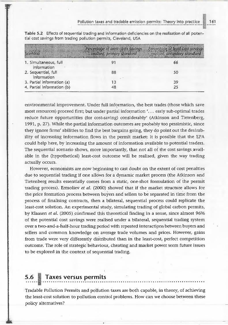
Table 5.2 ff t of sequential trading and inf rm tion ficiencies on .the rea lisation of all pot n-tial cost savings from trading pollution p rmit , Cl v land, USA

~11

1 . Simultaneous, full 91 66 information

2. Sequential, full 88 50 information

3. Partial information (a) 13 39 4. Partial information (b) 48 25

environmental improvement. Under full information, the best trades (those which save

most resources) proceed first; but under partial info~mation ' ... early sub-optimal trades

reduce future opportunities (for cost-saving) considerably' (Atkinson and Tietenberg, 1991, p. 27). While the.partial information outcomes are probably too pessimistic, since

they ignore firms' abilities to find the best bargains going, they do point out the desirab­

ility of increasing information flows in the permit market: it is possible that the EPA

could help here, by increasing the amount of information available to potential traders.

The sequential scenario shows, more importantly, that not all of t.he cost savings .avail­able in the (hypothetical) least-cost outcome will be realised, given the way trading

actually occurs.

However, economists are now beginning to cast doubt on the extent of cost penalties

due to sequential trading if one allows for a dynamic market process (the Atkinson and

Tietenberg results essentially comes from a static, one-shot formulation of the permit

trading process). Ermoliev et al. (2000) showed that if the market structure allows for

the price formation process between buyers and sellers to be separated in time from the

process of finalising contracts, then a bilateral, sequential process could replicate the

least-cost solution. An experimental study, simulating trading of global carbon permits,

by Klaasen et al. (2005) confirmed this theoretical finding in a sense, since almost 96%

of the potential cost savings were realised under a bilateral, sequential trading system

over a two-and-a-half-hour trading period with repeated interactipns between buyers and

sellers and common knowledge on average trade volumes and prices. However, gains

from trade were very differently distributed than in the least-cost, perfect competition

outcome. The role of strategic· behaviour, cheating and market power seem future issues

to be explored in the context of sequential trading.

5.6 , Taxes versus permits ~ ...... . i .................................................... ~ ....................... .

Tractable Pollution Permits and pollution taxes are both capable, in theory, of achieving

the least-cost solution to pollution control problems. How can we choose between these

policy alternatives?

161

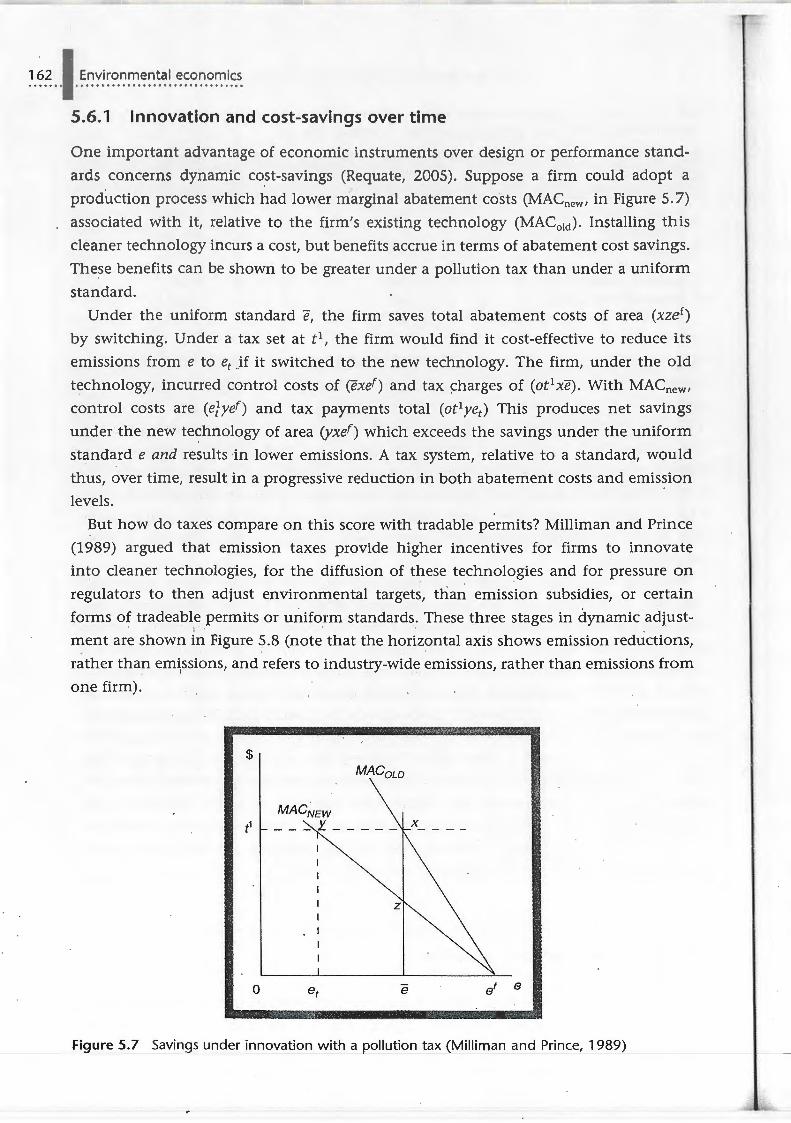
162 , nvironm nt I on mi ....... ' ....... .... ............. .... .. .. .

5.6.1 Innovation and cost-savings over time

ne important advantage of economi in trum nt v r design or performance stan -

ards concerns dynamic co.st-savings (R quat , 2005). Suppose a firm could adopt a

production pro ess which had lower marginal abatement costs (MACnew, in Figure 5. 7)

associated with it, relative to the firm's existing t chnology (MAC0 ,ct). Installing thi

cleaner technology incurs a cost, but benefits accrue in terms of abatement cost savings.

These benefits can be shown to be greater under a pollution tax than under a uniform

standard.

Under the uniform standard e, the firm saves total abatement costs of area (xzer)

by switching. Under a tax set at t1, the firm would find it cost-effective to reduce its

emissions from e to e1 .. if it switched to the new technology. The firm, under the old

technology, incurred control costs of (exef) and tax ~harges of (ot1 xe). With MACnew,

control costs are (ef yef) and tax payments total (ot 1ye1) This produces net savings

under the new technology of area (yxef) which exceeds the savings under the uniform

standard e and results in lower emissions. A tax system, relative to a standard, would

thus, over time, result in a progressive reduction in both abatement costs and emission

levels.

But how do taxes compare on this score with tractable permits? Milliman and Prince

(1989) argued that emission taxes provide higher incentives for firms to innovate

into cleaner technologies, for the diffusion of these technologies and for pressure on

regulators to then adjust environmental targets, than emission subsidies, or certain

forms of tradeable permits or uniform standards. These three stages in dynamic adjust­

ment are shown in Figure 5.8 (note that the horizontal axis shows emission reductions,

rather than em\ssions, and refers to industry-wide emissions, rather than emissions from

one firm).

$ MAC0 w

MACNEW t1 - - - r - - - - -

0 e e' e

Figure 5.7 Savings under innovation with a pollution tax (Milliman and Prince, 1989)

$

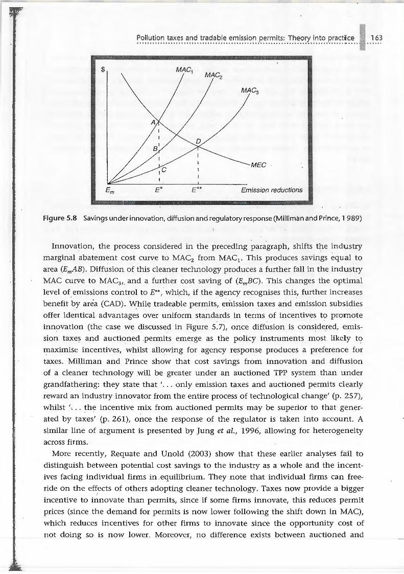
MEG

E* Emission reductions

Figure 5.8 Savings under innovation, diffusion and regulatory response (Milliman and Prince, 1 989)

Innovation, the process considered in the preceding paragraph, shifts t0e industry

marginal abatement cost curve to MAC2 from MAC1 . This produces savings equal to

area (E,,,AB). Diffusion of this cleaner technology produces a further fall in the industry

MAC curve to MAC3 , . and a further cost saving of (E,,,BC). This changes the optimal

level of. emissions control to E**, whi.ch, if the agency recognises this., further increases

benefit by area (CAD). ~hile tradeable permits, emission taxes and emission subsidies

offer identical advantages over uniform standards in terms of incentives to promote

innovation (the case we discussed in Figure 5.7), once diffusion is considered, emis­

sion taxes and auctioned .permits emerge as the policy instruments most likely t<?

maximise incentives, whilst allowing for agency re.sponse produces a preference for

taxes. Milliman and Prince show that cost savings from innovation and diffusion

of a cleaner technology will be greater under an auctioned TPP system than under

grandfathering: they state that ' ... only emission taxes and auctioned permits clearly

reward an industry innovator from the entire process of technological change' (p. 25 7),

whilst \ .. the incentive mix from auctioned permits may be superior to that gener­

ated by taxes' (p. 261), once the response of the regulator is taken into account. A

similar line of argument is presented by Jung et al., 1996, allowing for heterogeneity

across firms.

More recently, Requate and Unold (2003) show that these earlier analyses fail to

distinguish between potential cost savings to the industry as a whole and the incent­

ives facing individual firms in .equilibrium. They note that individual firms can free­

ride on the eft:ects of others adopting cleaner technology. Taxes now provide a bigger

incentive to innovate than permits, since if some firms innovate, this reduces permit

prices (since the demand for permits is now lower following the shift down in MAC),

which reduces incentives for other firms to innovate since the opportunity cost of

not doing so is now lower. Moreover, no difference exists between auctioned and

164 nvironm nomic

ra ndfalh r d p rmits in t rms f in ntiv t innovate. R quate and Un Ld fl

up ti imp rtan f another issu in thi s d bate over which instrum nt ncour-

ag s inn vati n b st: that of wheth r th nvironmental regulator anti ipates t

n w t chnol gy or not, and wh ther th y r - ommit to a change in nvironmental

pol_i y (in t rms of its type and its lev I) before the firms invest in cost-saving tech­

nol gy or not. The encouragement to r duce costs provided by market mechanisms

has been referred to as 'over the long haul, perhaps the most important criterion

on which to judge environmental policies' (Kneese and Schultze, 1978). Taxes seem

to do better than tractable permits in this important aspect of environmental policy

design.

5.6.2 Uncertainty

In Chapter 4, analysis was provided of how uncertainty over damage and control .costs

functions can complicate both the implementation of economic instruments and the

choice between them. What can be said about this issue in the specific context of the

relative merits of pollution taxes and tractable permits?

Pizer (1999, 2002) looks at this issue in the specific context of uncertainty over the

costs of controiHng GHG emissions. If there was no uncertainty over future control costs,

both tradeable quantity controls and carbon taxes would produce similar outcomes. But

considerable uncertainty does in fact exist, since (i) we have little experience with such

large cuts in ·emissions, (ii) we do not know what future technological options will be

and (iii) we do not know what the 'do nothing' level of emission will be, relative to

which achievements are measured and targets set.

Pizer constructs a scenario in which there is uncertainty over control costs, which then

turn out to be high.er than thought. With a permit system, emissions are unchanged

over the perfect information scenario, but costs of control rise. This stability of emission

in the face of uncertainty is one reason why TPPs are indeed favoured over taxes by some

environmental lobby groups (Stavins, 1998). Under a tax system, emissions are reduced

by less, but the price per ton of carbon stays constant. Permit systems thus result in more

uncertainty about costs than emission reductions, whilst this situation is reversed with

taxes. Pizer then subjects these alternatives to a run of 1000 qifferent predictions based

around current IPCC calculations. He finds that emissions are below the full-information

8.5 GtC (Giga tonnes of Carbon) level in 75% of cases with the tax, but exceed it in

the remaining cases. The permit market ensures that emissions never go above 8.5 Gt.

However, the same simulation of possible futm:e scenarios shows the costs of the permit

scheme to be in the range of 0-2.2% of global GDP, a much larger range than that for

the tax at 0.2-0.6% of global GDP. The variation of control costs is thus much greater

under the permit system than with a tax.

Which policy option should we choose? Pizer argues that it depends on what we

believe about damages. If there is some threshold beyond which further CO2 emissions

will impose very high (and maybe irreversible) costs, the greater certainty over emission

levels that comes with p rmil mark ts is pr f rabl . (f in st ad damages rise smoothly

with increasing emissions, t h thr ats a r not so bad, an d w p r f r the greater certa inty

over· control costs which m s fr m tax s. This pref r n for tax s over permits i r -

enforced when one rememb rs that it is not current emissi n that most worry us a ut

climate change, but the ov rail sto k of GHGs in the atmosph r , which changes v ry

slowly.

Pizer's more recent simulations reveal, by assuming the marginal benefits from G G

abatement schedule is relatively flat (which is what the literature tends to assume),

that a carbon tax increases welfare by five times the value achieved under tractab le

permits. What is more, he finds that the original Wietzman result, noted in Chapter 4, must be changed for stock pollution proble~ like climate cha._rige,· ~here costs ict~pen:d

on the current flow of pollution but damages (and thus the benefits of abatement)

depend on the stock. Now the taxes-versus-TPPs argument is no longer just about

the relative · slopes of the marginal cost and benefits of control functions - with

relatively flat marginal benefits favquring taxes - but must also _take into account

growth, depreciation, discounting and the correlation of shocks to the cost function over time.

Montero (1997) considers a rather different form of uncertainty, namely that over

whether the regulator will actually approve a proposed permit trade. In his model,

increasing uncertainty moves firms away from the overall least-cost solution. Firms may

indeed be uncertain about many aspects of future permit trading, including for instance

the effect of the number of permits they hold in the current round on the number they are grandfathered in subsequent rounds. The ability to be able to bank permits

for future use is a key factor in determining the extent to which such uncertainty

drives a wedge between the least-cost outcome and the actual trading outcome (Godby et al., 1997).

5.7 Why don't governments make more use of economic instruments for pollution control? ...... . ' ............................................................................ .

A conclusion which might be drawn from both the theoretical and the empirical studies

reported in this chapter is that economic instruments, such as taxes and TPPs, offer

the possibility of considerable efficiency gains over 'command-and-control' approaches

such as design and performance standards. However, as several recent surveys of actual

pollution control policy in the OECD have shown, governments have made relatively

little use of economic instruments as yet (OECD, 1997). Use of economic instruments has

certainly increased over time: this is evident if one compares earlier OECD surveys (e.g.

Opschoor and Vos, 1989) with more recent surveys, such as NCEE (2004; see Box 5.7) .

Major recent pieces of environmental legislation, such as the EU's Water Framework

Directive, actively encourage the wider use of economic instruments; whilst in the UK

the 1990s saw the introduction of several new economic instruments, such as a landfill

165

166 nvironmental economics

tax and a tax on aggregates extra t i n. We have also provided exampl s of current u~ s

f pollution taxes and tradabl p rmits in both the main text of this and the previo-us

hapt r, and in the box sections.

Recent experience in the use of economic instruments to control pollution

A report by the National Centre for Environmental Economics reviews experiences outside

the US with economic instruments for managing the environment, including air and water

quality, water quantity, solid and hazardous wastes. A comparison was drawn with a previous

EPA-funded survey in 1997. The main findings of the report were:

• Direct fees and taxes are the most used economic instruments internationally. Noteworthy

trends include more applications and higher rates, as well as some acceptance in parts of the

world where charges heretofore have been difficult to implement.

• Pollution permit trading regimes have gained greater acceptance worldwide, particularly for the

control of GHG emissions. New applications of marketable permits for conventional pollutants

in nations such as Chile, China and Slovakia are noted.

• Greenhouse gas emission control is an important and rapidly growing application of economic

instruments._ln 1997 just a handful of nations .imposed carbon taxes. Now many more nations

rely on carbon taxes and GHG trading regimes are in place ..

• Reductions in environmentally harmful subsidies has been encouraged by international lending I .

institutions. Leading lenders often make the elimination of environmentally harmful subsidies

a condition for lending.

• Liability for harms caused to the environment is increasingly being used as a tool to limit

polluting and environmentally damaging activities.

• Information is used in many new applications, including product labelling, categor­

ising firms according to their environmental performance and disclosure of pollution

releases.

• Voluntary programs now exist in a host of programmes to encourage firms to improve their

environmental performance. Much greater attention is also being paid to rewards that can

be offered in such programmes.

Overall, the report found a clear increase in the use of market mechanisms for environmental

protection worldwide, which is good news for environmental economists!

Yet the impression remains that economic instruments are still used rather less

than their theoretical advantages would seem to warrant. And even where economic

rr in trum nt ar br u rht in, Lhi is tim with th ma j r purp se of raising r ve u ,

rath r than hangin b havi ur (Harth Id, 1994).

Why? This questi n has b n inv stigated by many authors ( lahn, 1989; Cumberland,

1990; Hanl y et al., 1990; Ba rthho ld, 1994; Keohane et al., 1997; Stavins, 1998). An

early explanation was that f ignorance on th pa rt of policy-makers. Beckerman

(1975) suggested that the qiain reason economic instrum nts were not used was that

policy-makers were unaware of their potential. However, this is no longer true in th

OECD. The UK government, for example, has recently published several documents

supporting the concept of economic instruments (Department of the Environment,

1993), while economic instruments have been debated in the USA since the early 1970s (Nelson, 1987). ·

A second reason is practical problems. These include the use of either spatially

differentiated taxes or complex trading rules for non-uniformly mixed pollutants (for

instance, an ambient permit system has never been fmplemented, with the partial excep­

tion of the two-zone system used in the RECLAIM trading scheme in Los Angeles);

interactions between regulated pollutants, stochastic influences on pollution emis­

sions and resultant concentrations; and the way the regulator could reduce the supply of permits (or the level of pollution that a given supply permits) before the end

of the permits' expiry dates. For many water pollutants in many physical settings,

the potential number of traders in a TPP scheme is very small; whilst the finan­

cial transfers implicit in pure pollution tax schemes mitigate against their political acceptability.

A third possible reason is institutional problems. This is perhaps the most important

category. The logic behind a preference for economic instruments is that regulators

prefer more cost-effective policies to less cost~effective ones. Yet cost-effectiveness may

be ranked low by regulators in a list of policy objectives - although the Water Frame­

work Directive mentioned above places a specific duty on EU governments to design and

implement cost-effective catchment management plans for water quality. A second insti­

tutional problem is connected with the ethical implications of economic instruments.

Kelman (1981) has argued that pollution taxes, by putting a price on the right to pollute,

somehow debase the notion of environmental quality: his survey of the US environ­

mental lobby found that 68 per cent of those questioned took this view of pollution taxes

(interestingly, the same survey found that ·85 per cent of industrialists were opposed to

pollution taxes, on the grounds that these increased the financial burden on firms relative

to those imposed by the regulatory system). Tradeable permits could also be thought

of as 'rights to pollute' and thus also subject to ethical opposition from environmental

groups . .

Fourth, some economic instruments could actually increase the financial burdens

on firms, relative to command-and-control options, even- though they minimise

aggregate abatement costs from society's viewpoint. This is certainly very important

in any analysis of why pollution taxes at incentive rates have been so little

used (see Section 5.4), and is also an impediment to the introduction of auction-

1 7

168

b s d trad . bl p rmit h m . All wing firm s m l v of emissions ov r

which th y aP n t tax d, r using partial grandfath rin schemes, are both

ways around this pr bl m. It is interesting to n t in t his regard that a ll

izable tradeable p rmit syst m · implemented to dat ar grandfa thered rather th n

· auctioned.

Fina.Uy, both pollution tax s and TPPs are significant changes in pollution contro l

policy. Consequently, resistance can be expected from those with a vested inter t

in the preservation of th exis ting system, while bureaucracies in general m ay

resist wholesale changes in policy. It is interesting in this regard that some of the

best examples of economic instruments being introduced in the OECD are where

changes to the legislation are brought in gradually, rather than as a dramati c change. In Germany, for example, charge levels for water pollution were gradu­

ally increased over the first four years of the scheme. A related tactic to increase

firm approval is to introduce a voluntary scheme initially - this was the approach

taken in the UK to introducing the- concept of trading in CO2 emissions across

large point sources. It can also be the case that . industry will lobby in favour · of

economic instruments where it sees these as a way of saving costs over regulatory

alternatives.

As environmental standards become stricter, it is likely that the cost savings offered by

economic instruments will become more attractive to policy-makers. Indeed, industry

may make use of TPPs under its own initiatives, in order to reduce the costs of meeting

expected future legislation. A good example of this is the in-house trading system imple­

mented by BP in 1998, which covered GHG emissions from 150 BP units operating in

100 countries. In 2001, some 4.5 million .tonnes of emission reductions were traded

under this scheme worldwide (Akhurst et al., 2003). However, the lesson from the last

20 years is that most changes come gradually, that cost-savings can be over-estimated

by eager economists and that lobby groups will seek to retain regulation which is

relatively favourable to their own interests. As Stavins (1998) notes, the main reason

why command-and-control policies have dominated historically is ' ... because all of

the main parties involved had reasons to favour them: firms, environmental advocacy

groups, organised labour legislators and bureaucrats' (p. 72). Standards can improve

firms' competitive positions by protecting them from new entrants; can be more popular

with environmental lobby groups who find them easier environments in which to bring

their influence to bear than taxes or tractable permits, and who worry about localised

pollution problems emerging; are a more conducive working environment for regulators

trained in law rather than economics; and serve to partly hide the cost of environ­

mental standards from the public, unlike pollution taxes. Finally, Stavins notes that

regulators care more about the geographic; distribution of environmental costs and bene­

fits than their total cost-benefit effectiveness, which is the main selling point of economic

instruments.

REFERENCES

Akhur t, M., M Ph im, J. and T. wis, R. (2003) ' r nh us gas emissions trading in BP',

Energy Poli y, 31, 657- 663.

Atkinson, . and Ti t -nb rg, T. (1982) 'Th mpiri al properties of two classes of desi ns

for transf rabl dis hargc permits', Journal of Environmental Economics and Management, 9,

101- 121.

Atkinson, S. and Tie t nb rg, T. (1987) 'Economic implications of emissions trading rul s',

Canadian Journal of Economics, 20, 370- 386.

Atkinson, S. and Ti t nberg, T. (1991) 'Market failure in incentive based regulation:

The case of missions trading', Journal of Environmental Economics and Managem ent, · 21, 17-31.

Baumol, W . 'and Oates, W. (1971) 'The use of standards and prices for the protection. of the

environment', Swedish Journal of Economics, 73, 42- 54.

Baumol, ·W. and Oates, W. (1988) The Theory of Environmental Policy, 2nd edn. Cambridge: . . . Cambridge University Press.

Barthold, T.A. (1994) 'Issues in the design of environmental excise taxes', Journal of Economic

Perspectives, 8, 133- 151.

Beckerman, W. (1975) Pricing for Pollution. Londo~: Institute for Economic Affairs.

Bergman, L. (1991) 'General equilibrium effects of environmental policy', Environmental and

Resource Economics, 1(1), 43-63.

Boemare, C. and Quirion, P. (2002) 'Implementing greenhouse gas trading in Europe:

Lessons from economic literature and international experience', Ecological Economics,

43, 213-220.

Burtraw, D. (1999) 'Cost savings, market performance and economic benefits of the US acid

rain programme', in S. Sorrell and J. Skea (eds), Pollution for Sale: Emissions Trading and Joint

Implementation . Cheltenham: Edward Elgar.

Carlen, B. (2003) 'Market power in international carbon emissions trading', Working Paper,

MIT program on· Science and Policy of Climate Change.

Cason, T. (1993) 'Seller incentive properties of the EPA's emissions trading auction', Journal of

Environmental Economics and Management, 25, 177-195.

Cason, T. and Gangadharan L. (2003) 'Transactions costs in tractable permit markets', Joumal

of Regulatory Economics, 14(1), 55-73.

Cason, T., Gangadharan, L. and Duke, C. (2003) 'Market power in tractable emission markets:

A laboratory testbed for emission trading in Port Phillip Bay, Victoria', Ecological Economics,

46, 469-491.

Common, M. (1977) 'A note on the use of taxes to control pollution', Scandinavian Journal of

Economics, 79, 345-349.

Crampton, P. and Kerr, S. (1999) 'The distributional effects of carbon regulation: Why

auctioned permits are attractive and feasible', in T. Sterner (ed.), The Market and the Envir­

onment: The effectiveness of Market-Based Policy Instruments for Environmental Reform. Chel­

tenham: Edward Elgar.

Crocker, T. (1966) 'Structuring of atmospheric pollution control systems', in H. Wolozin (ed.),

The Economics of Air Pollution. New York: W.W. Norton.

Cumberland, J. (1990) 'Public choice and the improvement of policy instruments for envir­

onmental management', Ecological Economics, 2(2), 149-162.

1 9

170 nt I onomi

ales, J.H. (19 8) 1 oll11tio11, Property and Prices . T r nt : Univ rsity of Toronto Press.

partm n t f th Envir nm nt (1993) Makii18 Mark ls W ork for the Environment. Lond n :

HMSO.

Dresner, S. and Ekin , P. (2004a) 'The distributi nal impacts of economic instrumen ts

to limit gr nshouse gas emissions', Discussi n Paper 19, Policy Studies Institute,

London.

Dresner, S. and Ekins, P. (2004b) 'Economic instruments for a socially neutral national

home energy effici ency programme', Discussion Paper 18, Policy Studies Institute,

London.

Eheart, J., Joeres, E. and David, M. (1980) 'Distribution methods for transferable discharge

permits', Water Resources Research, 16, 833- 843.

Ellerman, A.O., Schmalensee, R., Joskow, P., Montero, J.-P. and Bailey, E. (1999) 'Summary

evaluation of the US S02 trading programme', in S. Sorrell and J. Skea .(eds), Pollution for

Sale: Emissions Trading and faint Implementation. Cheltenham: Edward Elgar.

Ellerman, A.O., Joskow, P.L. and Harrison, D. (2003) 'Emissions trading in the US: Experi­

ence, lessons and considerations for greenhouse gases', Pew Centre for Climate Change:

Washington, DC.

Ermoliev, Y., Nentjes, A. and Michalevich, 0. (2000) 'Markets for tradeable emission and

· ambient permits: A dynamic approach', Environmental and Resource Economics, 15, 39-56.

Fisher, AC (1980) Environmental and Resource Economics. Ca~bridge: Cambridge University

Press.

Godby, R., Mestelman, S., Muller, A.R. and Welland, J.D. (1997) 'Emissions trading with shares

· and coupons when control over damages is uncertain', fournal of Environmental Economics

and Management, 32, 359-381.

Godby, R. (2000) 'Market power and emission trading: Theory and laboratory results', Pacific

Economic Review, 5(3), 349-363.

Goulder, L., Parry, I. and Burtraw, D. (1997) 'Revenue-raising vs. other arproaches to envir­

onmental protection: The critical existence of pre-existing tax distortions', Rand fournal of

Economics, 28, 708-731.

Hahn, R. (1984) 'Market power and transferable property rights', Quarterly fournal of Economics,

99, 753-765.

Hahn, R. (1989) 'Economic prescriptions for environmental problems', fournal of Economic

Perspectives, 3, 95-114.

Hanley, N.D. and Moffatt, I. (1993) 'Efficiency and distributional aspects of market mechan­

isms in the control of pollution: An empirical analysis', Scottish foumal of Political Economy,

February, 40, 69-87.

Hanley, N., Moffatt, I. and Hallett, S. (1990) 'Why is more notice not taken of econom­

ists' prescriptions for the control of pollution?', Environment and Planning A, 22,

1421-1439.

Hanley, N., Faichney, R., Munro, A. and Shortle, J. (1998) 'Economic and environmental

modelling for pollution control in an estuary', fournal of Environmental Management, 52,

211-225.

Jensen, J. and Rasmussen, T. (2000) 'Allocation of CO2 permits: A general equilibrium

analysis of policy instruments', Journal of Environmental Economics and Management,

40(2), 111-136.

J sk w, P. . and hmal ns , R. (1 ) 'Th p liti a l n my f mark t-b s d

nvir nm ~n ta l p li y: Th U.S. a id rain pr gram', fournal of Law a11d £ onomi s,

41(1), ' 7- 83.

Jung, ., Krutill a, K. and Boyd, R. (1996) 'In ntives for advanced pollution abat m nt

techn logy at ti industry level', fournal of Environmental Economics and Managem ent,

30, 95- 111.

Kelman, S. (1981) 'Economists and the environmental policy mtiddle', Public Interest, 64,

106- 123.

Keohane, N. Revesz, R., and Stavins, R. (1997) 'The positive political economy of instrument

choice in environmental policy', in P. Portney and R. Shwab (eds), Environmental Economics

and Public Policy. Cheltenham: Edward Elgar.

Klaasen, G., Nentjes, A. and Smith, M. (2005) 'Testing the theory of emissions trading: Experi­

mental evidence on alternative mechanisms for global carbon trading', Ecological Economics,

53, 47-58.

Kling, C. (1994) 'Environmental benefits from marketable discharge permits', Ecological

Economics, 11(1), 57-64.

Kneese, A.V. and Schultze, C.L. (1978) Pollution Prices and Public Policy. Washington,. DC: Brookings Institute.

Kruger, J.A. and Pizer, W.A (2004) 'Greenhouse gas trading in Europe: The new grand policy

experiment', Environment, October, 46(8), 8-23.

Krupnick, A., Oates, W. and Van der-Verg, E. (1983) 'On the design of a market for air pollution

permits', Journal of Environmental Economics and Management, 10, 233-247.

Lyon, R. (1982) 'Auctions and alternative procedures for allocating pollution rights', La~d

Economics, 58, 16-32.

Maloney, M. and Yandle, B. (1984) 'Estimation of the 5ost of air pollution regulation', Journal

of Environmental Economics and Management, 11, 244-263.

McGartland, A. and Oates, W. (1985) 'Marketable permits for the prevention . of environmental deterioration', Journal of Environmental Economics and Management, 12,

207-228.

Michaelis, P. (1992). 'Global warming: Efficient policies in th_e case of multiple pollutants',

Environmental and Resource Economics, 2, 61-78.

Milliman, S.R. and Prince; R. (1989) 'Firm incentives to promote technological change in pollution control', Journal of Environmental Economics and Management,

17, 247-265.

Misiolek, W. and Elder, H. (1989) 'Exclusionary manipulation of markets for pollution rights',

Journal of Environmental Economics and Management, 16, 156-166.

Montero, J.-P. (1997) 'Marketable pollution permits with uncertainty and transactions costs',

.Resource and Energy Economics, 20, 27-50'.

Montgomery, W. (1972) 'Markets in licences and efficient pollution control programmes',

Journal of Economic Theory, 5, 395-418.

National Center for Environmental Economics (2004) International Experiences with Economic

Incentives for Protecting the Environment. Washington, DC: US Environmental Protection

Agency.

Nelson, R. (1987) 'The economics profession and the making of public policy', Journal of

Economic Literature, 25, 49-87.

1 72 nvironm

N tu ii, N .R. and Brad n, J .B. (2001) 'Transa t·i n sts and sequential barga ining in

trans£ rable dis ha rg p r111il mark ·', fournol of Environmental Manage111e11 t, 61 3),

253- 262.

ps t.ioor, J.B. and Vos, H.B. (1989) Econorni Instruments for Environmental Protection. Pa ·is:

ECO.

OE D (1997) Environmental Taxes and Green Tax Reform. Paris, OECD.

OECD (2000) Market Power and Market Access in International GHG Emission Trading.

Paris: OECD.

O'Neil, W., David, M., Moore, C. and Joeres, E. (1983) 'Transferable discharge permits and

economic efficiency: The Fox river', Journal of Environmental Economics and Management, 10,

346- 355.

Owen, A. and Hanley, N. (2004) The Economics of Climate Change. London: Routledge .

Pezzey, J.C. V. (1988) 'Market mechanisms of pollution control', in R.K. Turner ( ed .), Sustainable

Environmental Managem ent: Principles and Practice. London: Belhaven Press.

Pezzey, J.C.V. (1992) 'The symmetry between controlling pollution by price and controlling

it by quantity', Canadian Journal of Economics, 25(4), 983-991.

Pezzey, J.C.V. (2003) 'Emission taxes and tradeable permits: A comparison of views on long

run efficiency', Environmental and Resource Econom ics, 26(2), 329-342.

Pizer, W. (1999) 'Choosing price or quantity controls for greenhouse gases', Climate Issues

Brief no. 17, Resources for the Future.

Pizer, W. (2002) 'Combining Price and Quantity Controls to Mitigate Global Climate Change',

Journal of Public Economics, 85(3), 409-434.

Ribaudo, M., Heimlich, R. and Peters, M. (2005) ',Nitrogen sources and Gulf hypoxia: Potential

for environmental credit trading', Ecological Economics, 52(2), 159-168.

Requate, T. and Unold, W. (2003) 'Environmental policy incentives to adopt advanced abate­

ment technology: Will the true r~nk ing please stand up?', European Economic Review, 47,

125-146 .

. Requate, T. (2005) 'Dynamic incentives by environmental policy instruments: A survey', Ecolo­

gical Economics, 175-195.

Rowley, C., Beavis, B., McCabe, C. and Storey, D. (1979) A Study of Effluent Discharges to the

River Tees. London: Departm·ent of the Environment.

Schou, ].S. and Streibig, J.C. (1999) 'Pesticide taxes in Scandinavia', Pesticide Outlook, 10, 127-

129.

Schmalensee, R., Joskow, P., Ellerman, A.O. , Montero, J.-P. and Bailey, E. (1998) 'An interim

evaluation of the sulphur emissions trading programme', Journal of Economic Perspectives,

12(3), 53-68.

Seskin, E.P., Anderson, R.J. and Reid, R.O. (1983) 'An empirical analysis of economic strategies

for controllin& air pollution', Journal of Environmental Economics and Management, 10, 112-

124.

Stavins, R. (1995) 'Transactions costs and tradeable permits', Journal of Environmental Economics

and Management, 29, 133-148.

Stavins, R. (1998) 'What can we learn from the grand policy experiment? Lessons from S02

allowance trading', Journal of Economic Perspectives, 12(3), 69-88.

Tietenberg, T.H. (1973) 'Controlling pollution by price and standard systems: A general equi­

librium analysis', Swedish Journal of Economics, 75, 193-203.

Ti tenb r , T.H. (1974) 'On taxati n and lh ntr l of xtcrnaliti s: mm nt', Ameri m, fronomic Review, 64, 462- 466

Tietenb rg, T. (1984) 'Marketable missi n p rmits in principle and practic ', DP123, Wa h -ingt n, D : Resources for the Future.

Tietenberg, T. (1990) 'Economic instrum nts for environmental protection', Oxford Review of Economic Policy, 6(1), 17-33.

Vesterdal, M. and Svendson, G. (2004) 'How should greer:ihouse gas permits be allocated in the EU?' Energy Policy, 32, 961-968.

Walker, M. and Storey, D. (1977) 'The standards and prices approach to pbllution control: Problems of iteration', Scandinavian fournal of Economics, 79, 99- 109.

Weir, M., Birr-Pederson, K., Jacobsen, H. and Klok, J. (2005) 'Are CO2 taxes regressive? Evidence from the Danish experience', Ecological Economics, 52(2), 239- 252.

17