Embed Size (px)
Citation preview
Political Shirking − Proposition 13 vs. Proposition 8†
Seiji Fujii‡
Department of Economics University of California, Irvine
April 2, 2006
Abstract. This paper considers the efficiency of the political market in the California State legislature. I analyzed the property tax limitation voter initiative, Proposition 13. I found that districts which supported Proposition 13 more strongly were more likely to oppose the incumbents regardless of whether their preferences for property taxes were different from their districts. I also studied how legislators voted on the bills adopted after the passage of Proposition 13 to finance local governments. I found that legislators tended to follow the constituents’ will after they received the voters’ message expressed by the passage of Proposition 13
† I would like to thank Professor Amihai Glazer for innumerable advices, guidance and encouragement to write this paper. I would also thank Professor Jun Ishii, Professor Hiroki Kondo, Professor Aiji Tanaka, Professor Thomas McCaleb and the colleagues, Shuji Kimura and Yogesh Uppal, for helpful comments and suggestions. I am also grateful to the Department of Economics and the School of Social Sciences at UC-Irvine for financial support. All remaining errors are my own. ‡ Department of Economics, University of California at Irvine, Email: [email protected].
1 Introduction When political markets function well, legislators who poorly serve the constituents’
interests will sooner or later be voted out from office. Most empirical papers in the
shirking literature support and argue that political markets work efficiently and voters
successfully sort out politicians. Bender and Lott (1996) concludes that congressmen’s
voting patterns are very stable over time and do not show any indication of engaging in
the opportunistic behavior, and that even small deviations result in the politician being
removed from office.
Addressing questions of how shirking can be identified and measured, empirical
research papers propose the model of shirking as ideological consumption goods (Kau
and Rubin, 1979; Carson and Oppenheimer, 1984). However, this approach has suffered
both methodological and theoretical flaws; among others the underlying median voter
hypothesis does not always hold (Bender and Lott, 1996). In addition, the literature has
extensively focused on the US Congress, the Senate and the House of Representatives,
and overlooked state legislatures.
This paper considers Proposition 13 and the legislature’s alternative to Proposition 13,
Proposition 8 in the California state legislature in the late 1970’s. Since there was a clear
indication of different preferences for property taxes between the state legislators and the
constituents, the problem of identifying shirking politicians has already been solved.
Instead of applying the two-step residual approach in which shirking is interpreted as a
significant coefficient on the residual from the first-stage regression of ADA on
constituents’ characteristics in the second-stage regression of legislators’ voting, I
identify shirking politicians by looking at the roll call votes. Taking advantage of the
unique circumstance, this paper tests the efficiency of the political market at the local
level.
Analyzing the specific issue of property taxes has additional benefits. As Nelson and
Silberberg (1987) demonstrates, the cost of shirking is relatively higher on specific bills
on particular weapon systems with well-defined beneficiaries and relatively lower on
general defense expenditure bills with uncertain final distribution of funds, so that testing
a specific property tax bill from which homeowners receive benefits will become more
instructive. The test becomes efficient for yet another reason; property tax limitation was
1
an important issue in the 1970’s in California because of high inflation in the housing
market. Matsusaka (2004) argues that legislators might be in tune with their constituents
on high profile issues, but act against the constituents’ interests on less important issues
when voters do not have complete information and seldom have the choice of a candidate
with identical policy views along every dimension.
I also analyze the bills adopted after the passage of Proposition 13 to compensate for
the loss of millions of dollars in property tax collection which local agencies suffered.
Senate bill No. 154 (immediately followed by Senate bill No. 2212) is a short-run plan to
finance local governments, while Assembly bill 8 is a long-run plan. I ask how state
legislators reacted to the constituents’ message expressed by the passage of Proposition
13 when they voted on the bills. Applying the probit model, I test if state legislators from
districts which had strongly supported Proposition 13 voted differently on SB 154, SB
2212 and AB 8 than did legislators from districts which had only weekly supported
Proposition 13.
This paper proceeds as follows. The shirking literature is surveyed in section 2. Section
3 explains the background related to Propositions 13, Proposition 8, SB 154, SB 2212
and AB 8. Section 4 explains the data and method to test the hypotheses and discusses the
estimation results. Section 5 concludes.
2 Literature review “Shirking” means a lack of responsiveness by representatives to their constituents or the
failure by the legislators to act in the interests of their constituents (Bender and Lott, 1996;
Tien, 2001). To avoid being pejorative, it is also defined as actions taken by legislators
that do not benefit the group forming a specific constituency (Wright, 1993). This view of
political behavior is of importance only when a politician is thought of as an agent or a
mirror of the constituents (Tien, 2001). In this delegate or principal-agent model of
representation, politicians should follow the wishes of their constituents. On the other
hand, political shirking would not necessarily be a problem in the model of representation
2
which postulates that politicians should follow their own ideology to serve the
constituents’ interests.1
However, these definitions of shirking are still ambiguous. Are legislators supposed to
serve all the constituents in the district or a subset of them? A legislator’s geographic
constituency and reelection constituency can differ. A constituent could be defined as any
group or sets of groups including voters, contributors and party members that affect the
probability of reelection. Thus, the controversy centers around the problem of identifying
the precise composition of legislators’ constituents and the constituents’ interests. There
are two major different views of shirking, assuming different models of electoral
competition and the corresponding legislators’ incentive to shirk.
The first view of shirking is the ideology-as-a-consumption-good hypothesis in which
politicians compare the costs in the form of reduced probability of reelection and the
benefits from indulging in their own beliefs (Kau and Rubin, 1979; Carson and
Oppenheimer, 1984). Politicians have their own preferences that differ from those of their
constituents, which are assumed the interests of the median voter in their districts.
Maximizing the probability of reelection means taking the campaign position the median
voter most prefers. An alternative view of shirking is called the electoral support-
maximizing model or non-ideological shirking model in which politicians look at the
subset of the constituents for reelection and forsake the interests of the other constituents
in exchange for other forms of political support such as campaign contributions.
Politicians focus on the trade-offs between factors influencing only the probability of
reelection.
The literature supporting the ideology-as-a-consumption-good hypothesis has
considered the relationship between legislators’ voting and the costs of engaging in the
opportunistic behavior or the threat of reelection. One of the earlier research papers,
Nelson and Silberberg (1987) argues that the cost of shirking is relatively higher on
specific bills and relatively lower on general bills.2 The benefits from specific bills are
1 These concepts of representation are based on the original argument done by Edmond Burke, a representative in the British House of Commons in the 1770’s (Matsusaka, 2004; Tien, 2001). 2 Nelson and Silberberg compare general bills such as cutting defense spending by $33.3 billion for the fiscal years 1983-85 and specific bills such as cutting $180 million for Titan II intercontinental ballistic missiles in the fiscal year 1983.
3
well defined, and these kinds of bills will directly affect the wealth of individuals who
live in the affected district, whereas the final distribution of benefits on general bills is
generally not known when legislators vote. Incidentally, their findings suggest that the
test in my paper is more effective. Since the property tax is a more specific tax than other
kinds of taxes such as income or sales tax, voters’ reaction will be more sensitive to
legislators’ voting.
Other researchers consider how the cost of shirking changes when they do not face the
threat of reelection or when they serve their last term in office (Lott, 1987a). If politicians
decide to retire, they are more likely to shirk because voters can no longer punish them at
the following election. However, the literature shows that voting behavior of
representatives is very stable over time and they do not deviate from their constituents’
preferences even when they decide to retire. This suggests electoral competition properly
sorts politicians (Bender and Lott, 1996). In other words, the lack of empirical evidence
for a last-period problem supports the model of representation (Tien, 2001). By the time
legislators serve the last term, those who do not fit well the constituents have already
been voted out from office. Since a politician follows both his own ideology and their
constituents’ policy preferences when he votes, he will be lowering his own utility if he
attempts to deviate from the constituents’ interests during the last term. Thus, ideological
shirking will be of minor importance (Bender and Lott, 1996).3
The ideological consumption model is applied in a wide range of papers but is equally
challenged by many scholars. Two major disagreements among researchers are about (1)
the assumption of the median voter theory or the degree to which legislators alter their
voting behavior according to the change in the perceived costs and (2) the validity of the
two step procedure or the degree to which the first-stage residuals as the ideological
difference are artifacts. Based on the median voter theory, the typical empirical procedure
this model utilizes to identify a legislator’s shirking is the two-step residual approach;
First, ideological rating scores such as ADA scores are regressed on average
characteristics of the constituents of legislators’ political districts in the first stage; Next,
3 One might argue that the politicians shirk throughout their careers. To sort out this extreme hypothesis, Lott (1987a) looked at another measure of shirking and found the evidence that politicians reduce their attendance rates at their last term. If they do change voting behavior during the last period, there should be a movement in both dimensions.
4
the calculated residuals for each congressman rather than ADA scores itself is used as
one of the independent variables in the second-stage regression of legislator’s voting for a
bill; Then, a significant coefficient of the first-stage residuals in the second stage is
interpreted as voting on the bill influenced by legislator-specific ideology or shirking.
However, this interpretation is challenged by researchers. The underlying theoretical
model, the Downs median voter hypothesis, is often inconsistent with the common
phenomenon of a state having two senators with widely different ideological voting
records. In addition, the critique on the two-step methodological procedure argues that
the estimated residuals proxy for the ideology of legislators in the second stage represent
the omitted variables that could measure excluded constituents’ characteristics in the first
stage (Peltzman, 1984). To the extent that omitted constituent characteristics explain
legislators’ voting in the subsequent regression, the ideological proxy is correlated with
legislators’ voting patterns.
Since this paper starts from the fact that there was an ideological difference with
respect to property taxes between state legislators and voters in the 1970’s in California,
the difficult problem of how to identify shirking by specifying the relevant constituent
can be avoided. The question of how shirking is identified has already been solved
because the state legislators have a different opinion from the constituents on property
taxes in the case where the legislature attempted to head off Proposition 13 by placing a
more moderate alternative, Proposition 8, on the ballot. This point will be further
explained in the following section.
An alternative view of shirking is the electoral-support-maximizing model or non-
ideological shirking model. It is the subset of the constituents that the legislator serves,
and the deviation from the median voter’s policy preference does not imply shirking any
longer. Politicians simply make trade-offs between the factors influencing their
probability of reelection. Kau and Rubin (1993) argues that ideology and shirking should
be separated and non-ideological shirking is quite possible. In fact, they found evidence
that congressmen sometimes change their voting behavior in response to contributions.
However, earlier arguments on the last term shirking problem can also be applied to non-
ideological electoral-support-maximizing model. If campaign contributions do alter how
politicians vote, there should be instability in congressmen’s voting patterns with
5
congressmen changing their votes during their last term when campaign contribution
does not matter. If politicians have compromised their positions to receive contributions,
the decision not to seek reelection should remove the threat that displeasing contributors
bring and politicians are more likely to alter their voting behavior. But most empirical
papers indicate that the legislators’ voting records are quite stable over time. Although
campaign contributions may induce shirking, there is little evidence that political shirking
exists (Bender and Lott, 1996).
Therefore, both the ideology-as-a-consumption-good and the electoral-support-
maximizing models suggest that political shirking is not a problem. When politicians do
not serve the constituents’ interests, they will be defeated at the following election.
Political markets properly sorts politicians. In this sense the shirking literature is closely
related to the political market efficiency problem.
Matsusaka (2004) and Wright (1993) argue that political markets may not work well
when monitoring costs are high. Voters seldom have complete information about the
activities of particular politicians, but voters have to choose several politicians from the
governor to school board members from the ballot on Election Day. Since candidates take
positions on a large number of issues, the voter seldom has the choice of a candidate with
identical policy preferences on every dimension. Instead, the voter will weigh various
issues and choose the candidate who is closest “on average” to his ideal position or on a
few key issues. Thus, legislators might comply with the constituents’ preferences on high
profile issues, but act against the constituents’ interests on less visible or less important
issues (Matsusaka, 2004). This argument gives additional motivation to analyze
Proposition 13 because property tax limitation was so important an issue for both voters
and state legislators in California.
3 Background
3.1 Proposition 13 and Proposition 84
Proposition 13 limited the property tax rate to 1% of purchase price.5 Property tax
revenues, on which local governments rely, declined to less than half.6 Before
4 This section is mainly based on Kuttner (1980) and Rabushka and Ryan (1982).
6
Proposition 13 each local authority (counties, cities, school districts, and special districts)
had the power to determine how much property tax revenue to collect each year. Property
tax rates generally varied between 1.5 percent and 3.5 percent of market value and its
average was about 2.5 percent (O’Sullivan et al., 1995). Proposition 13 was a voter
initiative constitutional amendment and was approved by voters by a 2-1 margin at the
1978 primary election.7
There are several noteworthy political and economic features behind this major tax
revolt in California. The first point is the boomed housing market after the 1973-74
economic recession. Housing prices rose at 2-3 percent as in the rest of the country in the
mid-60’s, but by early 1976, they were rising at 2-3 percent a month. Many houses are
sold and resold before construction was complete and builders were not able to meet the
demand for housing. Inflation worsened as in other states during the 1970’s, but the gap
between home values and the general inflation rate was huge in California; single-family
home values increased by 6.1 percent, while overall prices rose by 3.3 percent in 1972;
they increased by 24.6 percent and 5.8 percent respectively in 1977. Although inflation
erodes consumer savings, housing became an attractive investment. Sometimes a third or
5 Proposition 13 specifies that; (1) the real property tax rate is limited to 1 % of the full cash value. (2) The full cash value of the property is its market value as of 1976 – 1977. (3) When there is a change of ownership, the property is reassessed at its market value. (4) The full cash value can increase with inflation up to 2% annually. And (5) state and local governments cannot impose any additional ad valorem taxes on real property. The state government also cannot impose any additional taxes without a two-thirds majority vote of the legislature. The city, county, and special district authorities cannot impose additional taxes without a two-thirds majority vote of the electorate. Proposition 13 was a constitutional amendment for article 13 and placed on the 13th position of the June ballot. 6 For example, county governments suffered a 52.3% decrease in general property tax revenue from the fiscal year of 1977-78 to 1978-79, whereas school and community college districts suffered a 53.1% decrease in property tax revenues. 7 The pre-Proposition 13 property tax limitation initiatives, Watson initiatives in 1968 and 1972, were both defeated by the legislature’s more moderate alternatives. Fischel (1996) and Matsusaka (2004) argue that the California voters changed their preferences for property taxes from liberal to conservative. Matsusaka demonstrates the preferences of California voters shifted to the right during the late 1960’s and 1970’s by showing steadily increasing approval rates for property tax limit initiatives. Fischel calculates a swing ratio as the percentage change in each city’s vote for the 1972 Watson initiative to the vote for Proposition 13. He then finds the property-rich districts disproportionately opposed the 1972 pre-Proposition 13 tax initiative but agreed to Proposition 13. One of the property-poor districts, Baldwin Park, swung 58%, while one of the property-rich districts, Beverly Hills, swung 154%. In addition, since the Vietnam War, the US citizens changed their political orientation from liberal to conservative. According to the opinion survey done by Ladd and Lipset, the percentage of people who said that the government wastes much of their tax money increased from 48 percent in 1964 to 74 percent in 1978. (Rabushka and Ryan; 1982)
7
a half of income was spent to buy a house. In the inflationary economy, spending a large
portion of one’s income in housing can be forced savings.
However, the financial situation could be seen differently to homeowners than to
politicians. Although some property taxes on individual homeowners doubled and tripled,
homes made up on average only about a third of the property tax base, and only a third of
properties was reassessed each year. Homeowners paid about 31.6 percent of state’s
property taxes in 1972, while they bore about 41.0 percent in 1977. Even though the
share of the tax burden shifted to homeowners, the state treasury was affected by a little
amount by property taxes. In fact, the percentage of total property tax revenues collected
in California during seventies actually decreased – from 7.2 percent of personal income
in 1972 to 6.5 percent in 1977. But since the state government raises its money mainly
from income and sales taxes, the budget surplus increased from about $¾ billion in 1975
to $4 billion in 1978. On the other hand, the California assessments of property values of
single-family houses increased by 110.9 percent between 1975 and 1978, the assessments
of apartments went up by 34.2 percent and commercial, industrial, farmland and public
utility assessments increased by 26.4 percent.
Income tax rates had not been raised since 1972 at the maximum rate of 11 percent on
taxable incomes exceeding $15500.8 But due to inflation, income tax collections soared.
As the inflationary economy stimulated consumer spending, even the state’s sales tax
receipts, though levied at a flat rate, increased substantially faster than real incomes.
Between 1974 and 1977, income taxes increased more than 150% and sales taxes
increased by 188%. In addition to this point, as assessed valuation went up, state aid for
schools, welfare, medical care, etc. went down. Tax burdens also shifted from state
revenue sources to local ones.
Inflation places taxpayers into higher tax brackets without increasing their disposable
incomes. With the “bracket creep” effect, Rabushka and Ryan (1982) argues that
“purchasing power of the California citizens, real disposable income per worker actually
8 Before 1967, the maximum income tax rate of 7 percent was imposed on taxable incomes exceeding $15000. In 1967 the rate raised to 10 percent on taxable incomes exceeding $14000. In 1971 the maximum rate increased to 11 percent on taxable incomes exceeding $14000.
8
decreased in 1976, 1977 and 1978.”9 California residents were paying one-third more in
state and local taxes as a share of personal income than were other states’ residents. Thus,
the bulk of the economic growth contributed only to government spending through taxes.
The proliferation of service districts at the local level almost guaranteed that the
taxpayers would be thoroughly confused about who was taxing them how much, and for
what. A taxpayer might find his property tax bill itemizing upward of twenty different
charges: a city tax, a county tax, one or two school taxes, and at least a dozen special
district taxes. Many local agencies have the autonomous power to levy taxes on property.
During the Depression, President Roosevelt encouraged governors to permit the creation
of special districts to carry out federally assisted public works. It turned out to politicians
that getting the voters to approve the creation of a special district is a lot easier than
persuading them to levy a new tax directly, even though the ultimate fiscal effect was the
same. This new form of local government often proved to be substantially less
accountable to the voters than a city council or county board of supervisors.
Everybody in Sacramento wanted a tax bill. Public pressure for substantial tax relief
due to massive property tax bills was one of the biggest issues in the 1977-78 Legislature.
But there were sharp divisions over how much the state treasury could afford and what
form the tax relief should take. This conflict caused the legislature to end up with no tax
relief measure during the 1977 legislative session. Jarvis and Gann, authors of
Proposition 13, succeeded partly because the legislature stalemated. Democratic Senator
Petris proposed a bill which raised capital gains taxes and produced the tax relief in lower
income brackets and was supported by a broad liberal coalition including labor, consumer
groups or local governments. Conservative Democrat Smith proposed a bill, which was
supported by the Republicans and the Governor, concentrated more of the relief in the
upper-income brackets and imposed a revenue limit on local government. Both proposals
failed.
Another issue was Serrano v. Priest. In 1971, the California Supreme court ruled in
Serrano that reliance on property taxes to finance public schools is unconstitutional and
9 Corrected for inflation by expressing all amount in 1967 dollars, real disposable income rose from $3199 in 1967 to $3836 in 1977 by about 20 percent. “Bracket creep” is the phenomenon in which the real after-tax income decreases due to the progressive tax system when personal income increases at the same rate as inflation.
9
violates the equal protection clause of the California constitution. The court required the
inequalities in dollar expenditures per student be limited within $100 across districts in
Serrano II in 1976. Fischel (1989, 1996, 2004) argues that the Serrano decision and the
legislature’s response to Serrano II, AB 65, caused Proposition 13 to pass; Serrano
violated the Tiebout system and higher-than-average-spending districts lost incentives to
preserve higher property tax rates. AB 65 was an expensive bill, and the legislature didn’t
afford to propose additional tax relief to homeowners.
By the beginning of the 1978 legislative session, the Jarvis and Gann’s initiative had
achieved far more than the required number of signatures to qualify for the June ballot,
and so the Legislature was well aware that Proposition 13 had a good chance to pass.
Governor Brown signed Senate Bill No.1 on March 3, 1978. SB 1 was called the Behr
bill, named after the chief author Senator Behr. SB 1 required a constitutional amendment
permitting “split roll tax rate,” that is, the different property tax rates for home and
business. Senate Constitutional Amendment No. 8 (SCA 8) placed Proposition 8 on the
June 1978 ballot to make SB 1 effective.10 Proposition 8 was the legislature’s more
moderate alternative to Proposition 13, and the state legislature attempted to head off
Proposition 13 by Proposition 8.11
Proposition 13 created a $6.15 billion tax relief, while it was estimated that Proposition
8 (SB 1) would create a $1.4 billion tax relief for homeowners and renters. For
homeowners, the bill provided a 30% reduction in property taxes or a $366 property tax
cut on average while maintaining homeowner exemption, $7000. For renters, who
consisted of about 45 percent of the electorate and did not receive any benefits from
Proposition 13, the bill increased the state income tax credit from $37 to $75 and allowed
welfare recipients to qualify for the credit. Senior citizens with income below $13,000
were granted additional relief. The Behr bill established separate tax rates between
10 I analyzed SCA 8 applying the same methods in section 4.1. But the results are qualitatively the same as SB 1. The estimation results are available upon request. 11 “Proposition 13 and Proposition 8 were mutually exclusive for voters. 20 percent of those who voted for Proposition 13 also voted for Proposition 8, while 91 percent who voted against Proposition 13 supported Proposition 8” (Rabushka and Ryan 1982). Fischel (2004) found that the correlation coefficient between the percentages of voters voted Yes on Proposition 13 and voted Yes on Proposition 8 by city level is negative 0.94. Cal. Stats. 1978, c. 24 specifies “This act (SB 1) shall be repealed on June 7, 1978, unless Proposition 8 on the ballot for the statewide election on June 6, 1978 is approved by the voters and Proposition 13 on the ballot for the statewide election on June 6, 1978 is rejected by the voters, or is declared unconstitutional by the courts."
10
residential and commercial construction. Since all property had to be treated equally
under the state constitution, SB 1 required a constitutional amendment to allow a split roll
tax system. Owners of single family houses would effectively be assessed at a lower
fraction of value than other commercial, industrial or farmland properties. The measure
limited revenues accruing to local government. A state revenue limit restricted future
state revenue growth to 1.2 times the annual percentage growth in state personal income.
And SB 1 automatically reduced homeowner tax rates when assessments rose.12 (Fischel,
1996; Kuttner, 1980; Rabushka and Ryan, 1982) Voters faced both propositions at the
1978 primary election and the choice was clear. The Behr bill would have taken effect
only if voters voted for Proposition 8 and against Proposition 13. Proposition 13 was
approved by 64.8% - 35.2% but Proposition 8 was rejected by 47% - 53%.
Business opposed Proposition 13 partly because property tax cuts might be offset with
new taxes on businesses. The potential damage to government could also hurt the
investment climate. Besides business, virtually every interest group formed a coalition to
oppose Proposition 13 on the ground that public schools might be closed when money ran
out, that police and fire services might be cut, or more simply that Proposition 13 is
worse than Proposition 8. Opponents came from labor, education, and political groups,
the press and politicians themselves. Among labor the opponents were, for example, the
AFL-CIO, the California Teachers Association and the California State Employee
Association. Among business the opponents were Bank of America, Atlantic Richfield
and Standard Oil. Among political groups the opponents were Common Cause, the
California PTA and the Democratic Party. Every major newspaper except the Los Angels
Herald Examiner opposed. Among politicians the opponents were the majority of state
legislators, the 58 county boards of supervisors, most mayors, school board members,
Governor Jerry Brown and two of the four Republican candidates for the governor. A
radio program reported seven past presidents of the American Economics Association
and 450 economists in colleges in California opposed. On the other hand, proponents
were a few economists including Milton Friedman, two other Republican candidates for
the governor and voters themselves, probably home owners. (Rabushka and Ryan, 1982)
12 The bill didn’t affect school funding. For school purposes, homeowners’ property remained fully taxable.
11
The vast majority of state legislators opposed Proposition 13. Those who opposed will
be identified by looking at roll call votes for SB 1 in the legislature.13 If a state legislator
voted “Yes” on SB 1, it will indicate the legislator is an opponent. As examples of roll
call votes, 6 State senators out of 40 voted “No” on SB 1 on January 30, 1978 and out of
80 Assembly members none of them voted “No” on SB 1 on March 2, 1978. See table 1.
3.2 SB 154 and AB 8 After the passage of Proposition 13, the legislature and the governor surveyed possible
damage on local governments due to the decline of property tax collection by more than
half.14 During only about three weeks between the passage of Proposition 13 and the next
fiscal year, the legislature and the governor managed to pass Senate bill No. 154
(immediately followed by Senate bill No. 2212). SB 154, popularly known as “Bailout I,”
specified a state bailout to local governments and offered a temporary solution. The bill
authorized $4.4 billion in relief to local governments to compensate the loss in property
taxes. School districts were to receive about $2.2 billion, the counties $1.48 billion, the
cities $250 million, and the special districts $125 million. $900 was set aside for short-
term loans to local governments.15 This measure was fashioned to meet most urgent
particular needs.
SB 154 provided about $2 billion of state assistance in the form of block grants and
provided for state assumption of the costs of several state-mandated health and welfare
programs. State aid increased in importance in the general county revenue from 23.9% in
1977-78 to 36% in 1978-79. The bill also specified the rule of allocating the 1% property
tax revenues collected by counties to local agencies for the fiscal year of 1978-79 on the
basis of their average share of county wide taxes over the previous three years. Block
grants for these local agencies were intended to insure that no local government would
13 The data on roll call votes of the California State Legislature come from “Journal of the Senate” and “Journal of the Assembly” issued by the Legislature. 14 The degrees in which local agencies rely on property taxes to finance public services vary from one agency to another. Some special districts have no source of revenue other than property taxes or related revenues such as an interest on property taxes, while counties rely about 30% before the passage of Proposition 13. 15 Some local authorities such as Alpine County or National City in LA County declined this state aid offer. (See Rabushka and Ryan p. 51)
12
experience in 1978-79 more than a 10% loss in total revenue for the fiscal year of 1977-
78.16
Assembly bill No. 8, on the other hand, specified a long-run bailout. This bill,
popularly known as “Bailout II,” authorized about $4.85 billion in 1979-80 and $5.5
billion in 1980-81. The bill eliminated the annual assistance but introduced a more
permanent source of revenue. The increase in property tax revenues due to growth in
assessed valuations was allocated to jurisdictions in which the property was located. AB
8 shifted a portion of property tax revenues from school districts to other local agencies
but increased financial assistance from state to school districts. Under AB 8 each local
agency receives a base allocation equal to the amount it received in the prior year plus its
share of additional revenues generated by the growth in assessed valuation within its
boundaries. As a 1979-80 base allocation counties received their 1978-79 share of
property taxes plus 100% of their 1978-79 block grant minus the state grant for county
health service. This measure was fashioned to prevent the state from attaching more
strings to regulate local government because Proposition 13 centralized the California
public sector by limiting the real property tax rate to 1%.17
Due to these bills, net losses were 6.1% for the general county revenues and 1.2% for
the general funds of school and community college districts respectively in the fiscal year
1978-79. The incomes in general funds for school and community college districts
increased by 10% from the fiscal year 1977-78 to the fiscal year 1979-80. On the other
hand, the general county revenue decreased by 2.8% from the fiscal year 1977-78 to
1979-80.
Regarding AB 8 implemented during 1979 legislative session, Rabshka and Ryan
(1982) found an interesting newspaper article: “Some senate opponents charged that it
was too generous with state revenues and amounted to “business-as-usual in Sacrament”
despite the tax-cutting message of Proposition 13” (San Francisco Chronicle 7/21/1979).
This newspaper article motivates this paper to take one step further, and in later section
16 However, since the legislature didn’t have enough information about special districts, the legislature gave county boards of supervisor total control or power over the allocation of the funds to special districts under SB 154. 17 Other supporters of the bill said that “within 5 years, schools in California would be in compliance with the Serrano decision, which required equal spending for each student in public schools.” (San Francisco Chronicle 7/21/1979)
13
4.2 I analyze how state legislators reacted to their districts’ preferences for property taxes
when they voted on SB 154, SB 2212 and AB 8. The article suggests that, although the
vast majority of state legislators opposed Proposition 13, legislators seemed to have
changed or revised their mind after they observed voters’ message expressed by the
passage of Proposition 13. This could indicate that the state legislators are an agent in the
delegate or principal-agent model of representation, which presumes that politicians
should follow the wishes of their constituents. In addition, since the legislature didn’t
increase property tax rates afterward, shirking might not be a problem and voters might
not need to punish their state legislators who initially didn’t represent constituents’
preferences.18
Some others argue that Proposition 13 moved political machine to the right. Few
politicians are willing to take public stands that go against the spirit of Proposition 13.
Governor Jerry Brown initially opposed Proposition 13 but later in his campaign he
announced “I was wrong.” He described himself as a “born again” tax cutter in the article
on September 6, 1978 in Los Angeles Times found by Rabshka and Ryan (1982).
4 Data, method, and estimation results
4.1 Shirking legislators Table 2 summarizes legislators’ voting results for the selected roll call vote on SB 1 and
electoral results on Proposition 13 by the senatorial and assembly district level on
Election Day. The roll call votes for SB 1 on Jan. 30, 1978 in the Senate and Mar. 2, 1978
in the Assembly are selected from table 1 because these floor votes are relatively more
important.
First, I look at which districts have different preferences for property taxes than the
state legislators, and which incumbents are defeated from those districts by just counting
the numbers. For the senatorial districts, 27 Senators out of total 40 districts voted “Yes”
and 6 Senators voted “No.” 2 Senators were absent and 4 Senators refrained from voting.
No information is available for Senator Carpenter from the 36th district. 37 senatorial
districts approved Proposition 13 and 3 districts denied. Thus, the State Senator and
voters had different preferences for property taxes in 25 districts, when the difference 18 Professor McCaleb pointed out this thought.
14
means that the district voted Yes on Proposition 13 and the legislator voted Yes on SB 1.
Looking at only incumbents who ran for the office at the following general elections, 2
incumbents out of the 19 districts were defeated. One incumbent was defeated when the
legislator refrained from voting and the district approved Proposition 13. One incumbent
was defeated at the next primary election. One incumbent was defeated at the 1978
primary when the legislator and the district had the different preferences.
Out of 80 assembly districts, 79 Assembly members voted “Yes” on the roll call vote
and one member was absent. 71 assembly districts approved Proposition 13 and 9
districts denied it. 70 assembly districts had different opinions between legislators and the
constituents. Looking at only incumbents who sought reelection at the 1978 general
election, 6 out of the 57 incumbents were removed from office. 2 incumbents were
defeated at the 1978 primary when the legislators and the districts had the different
preferences.
In short, 8 state legislators who sought reelection against their challengers were voted
out from office in the 76 districts where the district and the incumbent had the conflicting
opinions about Proposition 13.
Table 3 shows the percentages of state legislators who are reelected from 1972 to 1984
in California. As we can see, incumbents are generally safe over these years. As to the
Senate, the percentages fluctuate and there is no particular point to mention regarding
Proposition 13. However, we can see that relatively more incumbents in the Assembly
are defeated at the 1978 general election, although I do not apply any statistical methods
to analyze these numbers.
Next, I apply regression analyses to use the share of the two-party vote received by
incumbents to test how the incumbents fared in the following election if they didn’t
represent their constituents’ preferences for property taxes. The method relies on the
assumption that, if state legislators do not serve the constituents’ interests for property
taxes who are responsible to reelect them, they will lose the political support that helps
them hold office. I specify the political support measured by the percentage of the two-
party vote received by state legislators as a function of available explanatory variables.
The following is the explanation of the variables.
15
Dependent variable
Proportion (t): The percentage of the two-party vote received by each state legislator at
the general election after the passage of Proposition 13.19 The percentage of the two-party
vote is widely used to analyze the efficiency of political market in the literature. State
Senators are chosen for 4-year staggered terms and when they are from even- numbered
districts, I look at the 1978 general election results. When they are chosen from odd-
numbered districts, I look at the 1980 general election results. On the other hand, since
every Assembly member is chosen for 2-year terms every 2 years, I look at the 1978
general election. The sample includes only incumbents who sought reelection at both pre-
and post-Proposition 13 elections. The number of observations is 82. I omitted
observations in which the legislators did not seek reelection after the passage of
Proposition 13.20 I also excluded incumbents who were defeated at the 1978 primary
election.21 I also omitted the observations in which the incumbent had no opponent from
the other party.22
Independent variables
Yes: The dummy variable equals to 1 if the legislator voted Yes on SB 1 at the roll call
votes mentioned above. In the following OLS regression 19 Senators voted “Yes,” 3
Senators voted “No,” 2 Senators were absent, and 2 Senators refrained from voting, and
56 Assembly members voted “Yes.”
Prop 13: The percentage of voters who voted in favor of Proposition 13 in the
legislator’s district.23 This variable measures conservativeness of the constituents in terms
of property taxes. I assume that the higher percentage indicates the district is more
conservative with respect to property taxes. The districts’ preferences for property taxes
19 The data is taken from “Statement of Vote” issued by the California Secretary of State. 20 The legislators were retired in 2nd, 7th, 17th, 19th, 36th, and 38th senatorial districts and 42nd assembly district. The legislators ran for anther office in 30th, 31st, and 39th senatorial districts and 2nd, 4th, 5th, 10th, 13th, 20th, 30th, 33rd, 41st, 49th, 60th, 67th, 69th, 74th, and 76th assembly districts. 21 Incumbents were defeated in 26th senatorial and 57th and 61st assembly districts at the 1978 primary election. 22 Those observations for the variable Proportion (t) are 5th and 28th senatorial districts and 1st, 7th, 27th, 43rd and 63rd assembly districts. The observations for the variable Proportion (t-1) consist of 3rd and 14th senatorial districts and 11th assembly district. I also omitted 74th assembly district because there are two opponents from the other party. 23 The data is taken from “Statement of Vote” compiled by the California Secretary of State.
16
are represented by a continuous variable instead of a dichotomous variable in that the
former will measure the district’s preferences more precisely.
Democrat: Dummy variable equal to 1 if the incumbent is a Democrat.24 63 out of 82
state legislators are Democrats.
∆Party: The difference in party affiliation of voters in the legislator’s district before
and after the passage of Proposition 13, whose affiliation is the same as the incumbent.25
Seniority: The number of years the incumbent is in office.26 I count one year as 1 with
the base date of 12/31/1977.
Ideological difference: This variable will measure the general ideological difference
between legislators and their constituents.27 Ideological difference is the absolute
difference between District ideology and Legislator ideology divided by 100. Legislator
ideology and District ideology measure the general ideology of the incumbent and the
constituents respectively. Legislator ideology is the voting score which ranges between 0
and 100, representing the proportion of the time that a state legislator takes the
conservative position on roll call votes for environmental issues. The value of 100 means
the legislator is completely conservative. The scores are based on the last half of the
1977-78 session of the legislature. District ideology is the percentage of voters who voted
in favor of the Republican candidate for the Governor in the district at the 1978 general
election.
Proportion(t-1): The percentage of two-party vote received by the incumbent at the
general election before the passage of Proposition 13. For State Senators, I look at the
1974 general election if they come from the even-numbered district. If they are chosen in
the odd-numbered district, I look at the 1976 general election. For Assembly members, I
look at the 1976 general election.28 If there was no opponent from the other party, I look
at the 1974 general election.29
24 The information comes from “Statement of Vote” compiled by the California Secretary of State. 25 The data is taken form “Report of Registration” complied by the California Secretary of State. 26 The information comes from “California Legislature at Sacramento” complied by the legislature. 27 The voting score data come from the California League of Conservation Voters. The election results are retrieved from “Statement of Vote” compiled by the California Secretary of State. 28 I used the special elections in 22nd senatorial district held at 3/8/1977, in 44th assembly district held at 6/28/1977 and in 46th assembly district held at 6/21/1977. 29 Reapportionment occurred between 1972 and 1974.
17
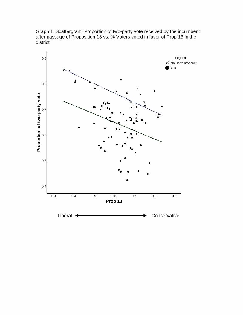
Graph 1 is a scattergram which shows a simple correlation or zero order correlation
between variables Proportion ( t) and Prop 13. There seems to be a negative relationship
between two variables overall. This graph also shows two separate lines fitted to two
groups of observations in which state legislators voted differently on the roll call votes on
SB 1. The solid line represents those who voted Yes on SB1, while the dashed line
represents those who voted No on SB1, refrained from voting or were absent. The solid
line is located below, while the dashed line is fitted above. Thus, the sample shows that
the proportion of two-party vote received by the incumbent declines if the variable Yes is
equal to 1 when the variable Prop13 increases. I test this difference shown in this sample
applying the OLS regression. The hypothesis that I test in this section is as follows:
Hypothesis 1: State legislators who did not represent the constituents’ preferences for
property taxes lost the electoral support more than other legislators who did represent the
constituents’ preferences.
The best way to estimate population parameters would be the Chow’s test of structural
change. One possible argument against this estimation is that the effect of shirking with
respect to Proposition 13 could disappear at the 1980 general election.30 Two years can
be long enough for voters to change the voting attitude toward a specific issue or change
an issue itself.31 However, there are possible explanations against this argument.
There are several propositions related to Proposition 13 submitted to voters after the
passage of Proposition 13. In November of 1979 there was an initiative, so-called Gann
“Spirit of Proposition 13” initiative sponsored by one of the same authors of Proposition
13, Paul Gann. Proposition 4 placed limits on state and local government spending. This
proposition was also approved by the voters, although this measure had little impact due
to the high rate of inflation. In addition, in June of 1980 there was an income-tax cutting
initiative, so-called “Jarvis II” or “Jaws II” named after one of the same authors of
30 Shuji Kimula pointed out this thought. 31 I analyzed only the incumbents who ran for reelection at the 1978 general election and omitted the observations of state senators from odd-numbered districts who ran at the 1980 general election. However, the estimation results turned out to be not significant. One explanation could be less variability in variables due to reducing the number of observations by 13.
18
Proposition 13, Howard Jarvis.32 Proposition 10 on the same ballot was to restrict rent-
control laws since tenants complained that they did not receive their fair share of
Proposition 13 savings. Both proposition s were rejected by the voters. In November of
1980, there were three propositions, which would modify Proposition 13 slightly.33 These
propositions, especially “Jaws II,” were salient enough for voters to remember
Proposition 13 and the effect of Proposition 13 on voters’ decision on how to vote would
remain.
Table 4 shows the results of the OLS regression with the Chow test. The results of fitting
models 1 – 3 would indicate that there is no structural break between two groups of
legislators who voted differently on SB1. Model 1 investigates if the break is due to the
intercept terms. Model 2 investigates if the break is due to the slope coefficients. And
model 3 investigates if the break is due to both the intercept terms and the slope
coefficients. None of the variables Yes and Yes×Prop13 is statistically significant in the
three regressions.
However, estimated coefficient on Prop 13 in model 4, which is negative and
statistically significant, indicates that the results suggest that districts punished every
incumbent regardless of whether they do not represent constituents’ preferences for
property taxes. Districts which supported Proposition 13 more strongly were more likely
to oppose the state legislature as a whole which attempted to defeat Proposition 13 by
Proposition 8.
This is quite rational when collecting information is costly.34 Instead of looking into
their state legislator’s voting on a specific bill, voters perceived the context in which
majority of state legislators, every interest group, most politicians including the governor
are confronting with homeowners. Since the legislature makes a decision under majority
rule, it is reasonable when districts punish the whole legislature which did not represent
the constituents’ preferences for property taxes. 32 Among others Proposition 9 proposed to cut state income tax rates in half or reduce from the progressive range of 1 to 11 percent to a new range of 0.5 to 5.5 percent. 33 Proposition 4, waiver of property-tax limits, was rejected. Proposition 5, reassessment of property, was also rejected. Proposition 7, solar-energy property taxation, was approved. 34 A related literature in political science is about “Issue voting” See Tanaka (1996) for the detail. There was a major argument over “whether an average voter can understand policy issues at the time of an election and whether he/she can make vote decision based on his/her issue attitude” (Tanaka; 1996).
19
But the magnitude to force them out from office would not be strong enough. When
Prop 13 increased by 1 percentage point, the percentage of two-party vote received by
the incumbents decreased by 0.236 percentage points on the average. This may appear
significant when the constituents increase the approval rates for property tax limitation by
10 percent and the race is very close with, say, a 51 – 49 margin. In this case the electoral
results could be reversed.
Among control variables, estimated coefficients on Democrat, Seniority and
Proportion(t-1) are statistically significant. The negative coefficient on Democrat
indicates that Democratic incumbents received lower support than Republican candidates
on the average. The negative coefficient on Seniority is not as expected. But the
magnitude is very small; when the incumbent holds his office longer by one year, he
loses his support by 0.0034 points on average or 0.34 percentage of the two-party vote he
received.
4.2 Agent legislators In the previous section I discussed how voters react when their state legislators did not
represent constituents’ preferences for property taxes and we have seen that voters punish
all state legislators regardless of whether they shirked or not. In this section I consider
how state legislators voted in the legislature after they observed their constituents’
conservativeness in terms of property taxes. As I mentioned in section 3.2, after
legislators observed the voters’ wishes expressed by the passage of Proposition 13,
legislators seemed to follow the voters’ message when they voted on AB 8. The
newspaper article in section 3.2 clearly indicates this attitude of state legislators: “Some
senate opponents charged that it (AB 8) was too generous with state revenues and
amounted to “business-as-usual in Sacrament” despite the tax-cutting message of
Proposition 13” (San Francisco Chronicle 7/21/1979).
In this section I analyze the roll call votes on SB 154, SB 2212 and AB 8 discussed in
section 3.2 to examine how state legislators reacted the constituents’ preferences for
property taxes.35 I test the second hypothesis that legislators from districts which had
strongly supported Proposition 13 voted differently on SB 154, SB 2212 and AB 8 than 35 The brief roll call vote results for these bills are in table 1.
20
did legislators from districts which had only weekly supported Proposition 13, applying
the probit regression.
I use the same independent variables in the analyses on SB 154 and SB 2212 but
slightly different variables in the analysis of AB 8. The number of observations for the
analyses of SB 154 and SB 2212 is 116.36 It is 118 for the analysis of AB 8.37
Dependent variable is a dichotomous variable which takes on the value of one if the
legislator voted Yes on the bills. For the analysis of SB 154 I looked at the roll calls both
in the Senate and the Assembly on June 23, 1978. 32 Senators voted “Yes” on this bill, 2
Senators were absent at this roll call, and 1 Senator refrained from voting. 3 Senators
voted against it. 76 Assembly members voted “Yes” and 2 members voted against it.
For the analysis of SB 2212, I look at the roll call votes both in the Senate and the
Assembly on June 30, 1978. 25 Senators voted “Yes,” 3 Senators were absent, and 3
senators refrained from voting on this bill. 7 Senators voted “No.” 59 Assembly members
voted “Yes,” 16 voted “No,” and 3 refrained from voting.
In the analysis of AB 8 I look at the roll call vote on July 19, 1979 for the Assembly
and July 20, 1979 for the Senate. 27 Senators voted “Yes” and 12 Senators voted “No.”
69 Assembly members voted “Yes” and 10 members voted “No” on this bill.
Independent variable
Prop 13: The same as in section 4.1.
Democrat: The same as in section 4.1. There were 79 democrats in the analysis of
SB154 and SB 2212 and 73 democrats in the analysis of AB 8.
Proportion(t-1): The same as in section 4.1 for the analysis of SB 154 and SB 2212. In
the analysis of AB8 I look at the 1978 general election for the Senator from even-
numbered districts and all the Assembly members and look at the 1976 general election
for the Senator from odd-numbered districts.
36 3rd and 14th senatorial districts and 11th and 74th assembly districts are omitted because the proportion of two-party vote is not available. 37 3rd senatorial district and 64th assembly district are omitted because the proportion of two-party vote is not available.
21
Seniority: The same as in section 4.1 for the analysis of SB 154 and SB 2212. In the
analysis of AB 8 I used 12/31/1978 as the base year and count one year as 1.
Legislator ideology is explained in section 4.1. For the analysis of SB 154 and SB
2212 I used the same variables in section 4.1. But in the analysis of AB 8 I look at the
voting scores from the League of Conservation Voters based on the last half of the 1979-
80 session of the legislature. I standardized the voting scores to estimate the score of
Senator Smith from 12th district, using the 1979 session voting scores, because the
legislator’s score is not available.
District ideology is the same as in section 4.1.
Last term 1 is the dummy variable equals to 1 if the legislator was retiring.
Last term 2 is the dummy variable equals to 1 if the legislator faces the last term but
ran for another office or was appointed to another office subject to election later.
Table 5 shows the estimation results of applying the probit estimation. I analyze SB 154,
SB 2212 and AB 8. As the estimated coefficients on variable Prop 13 in the three
regressions indicate, state legislators still did not match the constituents’ preferences for
property taxes when they voted on the short-run rescue bills but they did represent the
constituents’ preference when they voted on the long-run assistance bill. The estimated
coefficient on Prop 13 in the third model is negative and statistically significant, which
suggests that the probability of legislators voting on AB 8 decreases when Prop 13
increases by one percentage point. Legislators from districts which had strongly
supported Proposition 13 voted more likely against AB 8 than did legislators from
districts which had only weekly supported Proposition 13.
This finding is consistent with the former newspaper article which states some
legislators revised their opinion about property taxes after they received tax-cutting
message from their constituents. It is also consistent with other findings in the shirking
literature, which argue that elected politicians represent the constituents’ preferences.
5 Conclusion This paper considers the efficiency of the political market at the California state level in
the context of the famous tax revolt. As the roll call votes on SB 1 and the electoral
22
results for Proposition 13 indicate that the state legislators and the constituents had
different preferences for property taxes, this paper tests the hypothesis that voters
successfully sort out the shirking politicians. The results show that the districts punished
the legislature as a whole regardless of whether their representative represents the
constituent’s preferences for property taxes.
Applying the probit model to the roll call votes on the bills to support local
governments’ finance after the passage of Proposition 13, I also found that the state
legislators take into consideration their districts’ preferences for property taxes when they
vote on the bills. This finding suggests that after legislators observed the message
conveyed by the passage of Proposition 13, they followed the constituents’ will.
This paper does not ask a question of being right or being wrong. But there are mainly
three reasons why Proposition 13 could be worse than Proposition 8.38 Because of these
reasons, state legislators might oppose Proposition 13 and intend to defeat it by the
legislature’s more moderate alternative, Proposition 8. Proposition 13 has taken effect for
more than 25 years as the California constitution. We must keep in mind that, if the
majority of voters or the majority of voters who voted were misguided, the state could go
in a wrong direction.39
References Bender, Bruce and John R. Lott, Jr., “Legislator voting and shirking: A critical review of
the literature,” Public Choice, 87, 1996, pp67-100. California. Legislature, California Legislature at Sacramento, Sacramento, Various years. California. Legislature, Journal of the Assembly, Legislature of the State of California,
1977/78 Regular Session, Available at: http://www.assembly.ca.gov/clerk/billslegislature/srchframe.htm.
California. Legislature, Journal of the Senate, Legislature of the State of California, 1977/78 Regular Session, Sacramento.
38 (1) About $3.5 billion out of $5.5 billion savings would go to landlords and business property and mostly to out-of-state corporate shareholders. State and federal government would recapture over $1.5 billion due to diminished property tax deductions against the income tax. In short, Proposition 13 removed $5.5 billion worth of revenues but saved homeowners only about $2 billion in taxes. (2) Tax burdens were shifted from the old to the young. Property assessments were rolled back and frozen at the 1975-76 level. Only newly bought homes are assessed at the current market price. Thus, two identical homes located next to each other could be assessed quite differently. With this locked-in assessment, nobody would want to buy a house. (3) Tax burdens were shifted from business to homeowners. Factories and refineries are almost never sold compared to homes. “In addition, sales of business properties are often missed by the assessor because the transfer is of stock rather than the physical property.” (Kuttner 1980) 39 Turnout rate in terms of registered voters at the 1978 primary election was 68.9%. (Statement of vote)
23
California. Legislature, Senate Final History, 1977/78 Regular Session, Sacramento. California. Legislature, Assembly Final History, 1979/80 Regular Session, Sacramento. California Center for Research and Education in Government, California Journal,
Sacramento, Various months and years. California League of Conservation Voters, Voting Record, San Francisco, Various years. California. Secretary of State. Report of Registration, Sacramento, Various years. California. Secretary of State. Statement of Vote, Sacramento, Various years. California. State Controller, Annual Report of Financial Transactions concerning
Counties of California, Sacramento, Fiscal years 1978-79 and 1979-80. California. State Controller, Annual Report of Financial Transactions concerning School
Districts of California, Sacramento, Fiscal years 1978-79 and 1979-80. Carson, Richard T. and Joe A. Oppenheimer, “A Model of Estimating the Personal
Ideology of Political Representatives,” American Political Science Review, 78, 1984, pp163-178.
Downs, Anthony. An Economic Theory of Democracy, 1957, Harper & Row Publishers, New York.
Fischel, William A., “Did Serrano Cause Proposition 13?” National Tax Journal, 42, 1989, pp465-473.
Fischel, William A., “Did Serrano Vote For Proposition 13? A Reply to Stark and Zasloff’s “Tiebout and Tax Revolts: Did Serrano Really Cause Proposition 13?”” UCLA Law Review, 51, 2004, pp887-928.
Fischel, William A., “How Serrano Caused Proposition 13?” Journal of Law and Politics, 12, 1996, pp607-636.
Kau, James B. and Paul H. Rubin, “Self-interest, ideology, and logrolling in congressional voting,” Journal of Law and Economics, 22, 1979, pp365-384.
Kau, James B. and Paul H. Rubin, “Ideology, voting, and shirking,” Public Choice, 76, 1993, pp151-172.
Kutter, Robert, Revolt of the Haves: Tax Rebellion and Hard Times, Simon and Schuster (New York), 1980.
Lott, John R., Jr., “Political cheating,” Public Choice, 52, 1987, pp169-186. Matsusaka, John G., For the Many or the Few: The Initiative, Public Policy, and
American Democracy (American Politics and Political Economy Series), University of Chicago Press (Chicago), 2004.
Nelson, Douglas and Eugene Silberberg, “Ideology and Legislator Shirking,” Economic Inquiry, 25, 1987, pp15-25.
O’Sullivan, Arthur, Terri Sexton and Steven Sheffrin, Property taxes and the revolts: The legacy of Proposition 13, Cambridge University Press (Cambridge), 1994.
Rabushka, Alvin and Pauline Ryan, The Tax Revolt, Hoover Institution (Stanford), 1982. Tanaka, Aiji, “Issue Voting,” Japanese Journal of Electoral Studies, 13, 1998, pp17-27. Tien, Charles, “Representation, voluntary retirement, and shirking in the last term,”
Public Choice, 106, 2001, pp117-130. Wright, Matthew B., “Shirking and political support in the U.S. Senate, 1964–1984,”
Public Choice, 76, 1993, pp103-123.
24
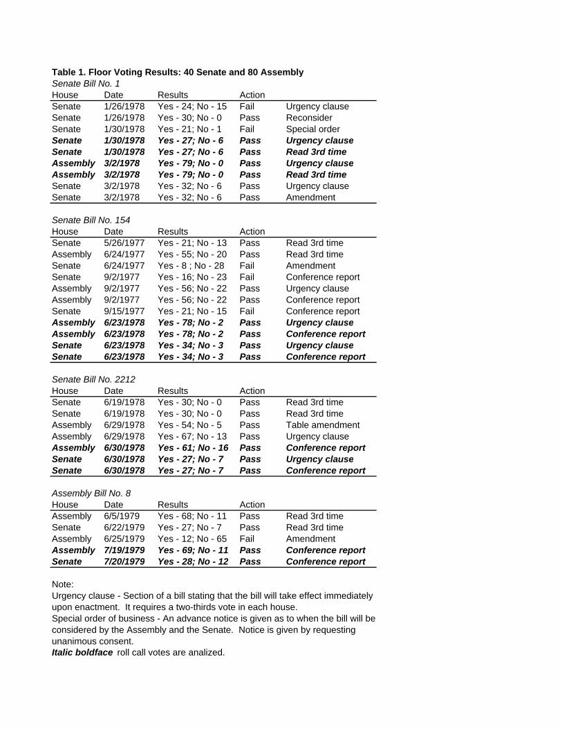
Table 1. Floor Voting Results: 40 Senate and 80 AssemblySenate Bill No. 1House Date Results ActionSenate 1/26/1978 Yes - 24; No - 15 Fail Urgency clauseSenate 1/26/1978 Yes - 30; No - 0 Pass ReconsiderSenate 1/30/1978 Yes - 21; No - 1 Fail Special orderSenate 1/30/1978 Yes - 27; No - 6 Pass Urgency clauseSenate 1/30/1978 Yes - 27; No - 6 Pass Read 3rd timeAssembly 3/2/1978 Yes - 79; No - 0 Pass Urgency clauseAssembly 3/2/1978 Yes - 79; No - 0 Pass Read 3rd timeSenate 3/2/1978 Yes - 32; No - 6 Pass Urgency clauseSenate 3/2/1978 Yes - 32; No - 6 Pass Amendment
Senate Bill No. 154House Date Results ActionSenate 5/26/1977 Yes - 21; No - 13 Pass Read 3rd timeAssembly 6/24/1977 Yes - 55; No - 20 Pass Read 3rd timeSenate 6/24/1977 Yes - 8 ; No - 28 Fail AmendmentSenate 9/2/1977 Yes - 16; No - 23 Fail Conference reportAssembly 9/2/1977 Yes - 56; No - 22 Pass Urgency clause Assembly 9/2/1977 Yes - 56; No - 22 Pass Conference reportSenate 9/15/1977 Yes - 21; No - 15 Fail Conference reportAssembly 6/23/1978 Yes - 78; No - 2 Pass Urgency clauseAssembly 6/23/1978 Yes - 78; No - 2 Pass Conference reportSenate 6/23/1978 Yes - 34; No - 3 Pass Urgency clauseSenate 6/23/1978 Yes - 34; No - 3 Pass Conference report
Senate Bill No. 2212House Date Results ActionSenate 6/19/1978 Yes - 30; No - 0 Pass Read 3rd timeSenate 6/19/1978 Yes - 30; No - 0 Pass Read 3rd timeAssembly 6/29/1978 Yes - 54; No - 5 Pass Table amendmentAssembly 6/29/1978 Yes - 67; No - 13 Pass Urgency clauseAssembly 6/30/1978 Yes - 61; No - 16 Pass Conference reportSenate 6/30/1978 Yes - 27; No - 7 Pass Urgency clauseSenate 6/30/1978 Yes - 27; No - 7 Pass Conference report
Assembly Bill No. 8House Date Results ActionAssembly 6/5/1979 Yes - 68; No - 11 Pass Read 3rd timeSenate 6/22/1979 Yes - 27; No - 7 Pass Read 3rd timeAssembly 6/25/1979 Yes - 12; No - 65 Fail AmendmentAssembly 7/19/1979 Yes - 69; No - 11 Pass Conference reportSenate 7/20/1979 Yes - 28; No - 12 Pass Conference report
Note:Urgency clause - Section of a bill stating that the bill will take effect immediatelyupon enactment. It requires a two-thirds vote in each house.Special order of business - An advance notice is given as to when the bill will be considered by the Assembly and the Senate. Notice is given by requestingunanimous consent.Italic boldface roll call votes are analized.
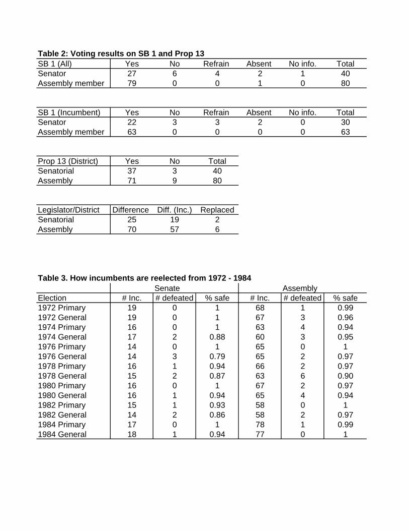
Table 2: Voting results on SB 1 and Prop 13SB 1 (All) Yes No Refrain Absent No info. TotalSenator 27 6 4 2 1 40Assembly member 79 0 0 1 0 80
SB 1 (Incumbent) Yes No Refrain Absent No info. TotalSenator 22 3 3 2 0 30Assembly member 63 0 0 0 0 63
Prop 13 (District) Yes No TotalSenatorial 37 3 40Assembly 71 9 80
Legislator/District Difference Diff. (Inc.) ReplacedSenatorial 25 19 2Assembly 70 57 6
Table 3. How incumbents are reelected from 1972 - 1984Senate Assembly
Election # Inc. # defeated % safe # Inc. # defeated % safe1972 Primary 19 0 1 68 1 0.991972 General 19 0 1 67 3 0.961974 Primary 16 0 1 63 4 0.941974 General 17 2 0.88 60 3 0.951976 Primary 14 0 1 65 0 11976 General 14 3 0.79 65 2 0.971978 Primary 16 1 0.94 66 2 0.971978 General 15 2 0.87 63 6 0.901980 Primary 16 0 1 67 2 0.971980 General 16 1 0.94 65 4 0.941982 Primary 15 1 0.93 58 0 11982 General 14 2 0.86 58 2 0.971984 Primary 17 0 1 78 1 0.991984 General 18 1 0.94 77 0 1
Graph 1. Scattergram: Proportion of two-party vote received by the incumbent after passage of Proposition 13 vs. % Voters voted in favor of Prop 13 in the district
0.3 0.4 0.5 0.6 0.7 0.8 0.9
Prop 13
0.4
0.5
0.6
0.7
0.8
0.9
Prop
ortio
n of
two-
part
y vo
te
LegendNo/Refrain/AbsentYes
Liberal Conservative
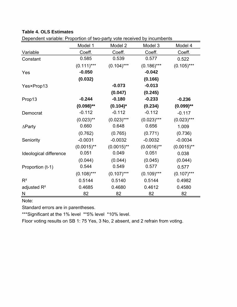
Table 4. OLS Estimates Dependent variable: Proportion of two-party vote received by incumbents
Model 1 Model 2 Model 3 Model 4Variable Coeff. Coeff. Coeff. Coeff.Constant 0.585 0.539 0.577 0.522
(0.111)*** (0.104)*** (0.186)*** (0.105)***Yes -0.050 -0.042
(0.032) (0.166)Yes×Prop13 -0.073 -0.013
(0.047) (0.245)Prop13 -0.244 -0.180 -0.233 -0.236
(0.098)** (0.104)* (0.234) (0.099)**Democrat -0.112 -0.112 -0.112 -0.117
(0.023)** (0.023)*** (0.023)*** (0.023)***∆Party 0.660 0.648 0.656 1.009
(0.762) (0.765) (0.771) (0.736)Seniority -0.0031 -0.0032 -0.0032 -0.0034
(0.0015)** (0.0015)** (0.0016)** (0.0015)**Ideological difference 0.051 0.049 0.051 0.038
(0.044) (0.044) (0.045) (0.044)Proportion (t-1) 0.544 0.549 0.577 0.577
(0.108)*** (0.107)*** (0.109)*** (0.107)***R² 0.5144 0.5140 0.5144 0.4982adjusted R² 0.4685 0.4680 0.4612 0.4580N 82 82 82 82Note: Standard errors are in parentheses.***Significant at the 1% level **5% level *10% level.Floor voting results on SB 1: 75 Yes, 3 No, 2 absent, and 2 refrain from voting.
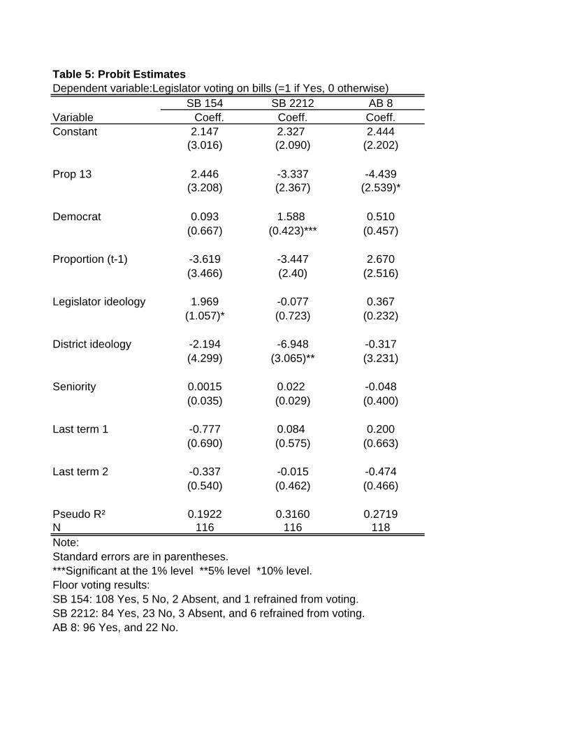
Table 5: Probit EstimatesDependent variable:Legislator voting on bills (=1 if Yes, 0 otherwise)
SB 154 SB 2212 AB 8Variable Coeff. Coeff. Coeff.Constant 2.147 2.327 2.444
(3.016) (2.090) (2.202)
Prop 13 2.446 -3.337 -4.439(3.208) (2.367) (2.539)*
Democrat 0.093 1.588 0.510(0.667) (0.423)*** (0.457)
Proportion (t-1) -3.619 -3.447 2.670(3.466) (2.40) (2.516)
Legislator ideology 1.969 -0.077 0.367(1.057)* (0.723) (0.232)
District ideology -2.194 -6.948 -0.317(4.299) (3.065)** (3.231)
Seniority 0.0015 0.022 -0.048(0.035) (0.029) (0.400)
Last term 1 -0.777 0.084 0.200(0.690) (0.575) (0.663)
Last term 2 -0.337 -0.015 -0.474(0.540) (0.462) (0.466)
Pseudo R² 0.1922 0.3160 0.2719N 116 116 118Note: Standard errors are in parentheses.***Significant at the 1% level **5% level *10% level.Floor voting results:SB 154: 108 Yes, 5 No, 2 Absent, and 1 refrained from voting.SB 2212: 84 Yes, 23 No, 3 Absent, and 6 refrained from voting.AB 8: 96 Yes, and 22 No.
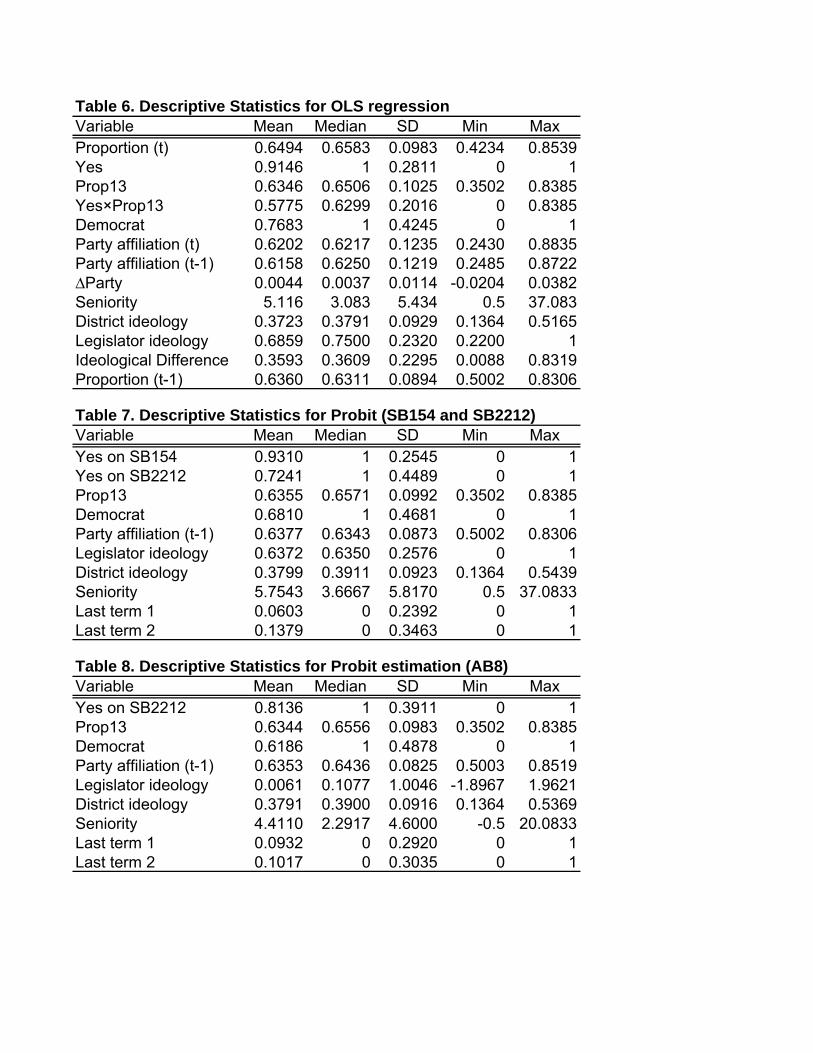
Table 6. Descriptive Statistics for OLS regressionVariable Mean Median SD Min MaxProportion (t) 0.6494 0.6583 0.0983 0.4234 0.8539Yes 0.9146 1 0.2811 0 1Prop13 0.6346 0.6506 0.1025 0.3502 0.8385Yes×Prop13 0.5775 0.6299 0.2016 0 0.8385Democrat 0.7683 1 0.4245 0 1Party affiliation (t) 0.6202 0.6217 0.1235 0.2430 0.8835Party affiliation (t-1) 0.6158 0.6250 0.1219 0.2485 0.8722∆Party 0.0044 0.0037 0.0114 -0.0204 0.0382Seniority 5.116 3.083 5.434 0.5 37.083District ideology 0.3723 0.3791 0.0929 0.1364 0.5165Legislator ideology 0.6859 0.7500 0.2320 0.2200 1Ideological Difference 0.3593 0.3609 0.2295 0.0088 0.8319Proportion (t-1) 0.6360 0.6311 0.0894 0.5002 0.8306
Table 7. Descriptive Statistics for Probit (SB154 and SB2212)Variable Mean Median SD Min MaxYes on SB154 0.9310 1 0.2545 0 1Yes on SB2212 0.7241 1 0.4489 0 1Prop13 0.6355 0.6571 0.0992 0.3502 0.8385Democrat 0.6810 1 0.4681 0 1Party affiliation (t-1) 0.6377 0.6343 0.0873 0.5002 0.8306Legislator ideology 0.6372 0.6350 0.2576 0 1District ideology 0.3799 0.3911 0.0923 0.1364 0.5439Seniority 5.7543 3.6667 5.8170 0.5 37.0833Last term 1 0.0603 0 0.2392 0 1Last term 2 0.1379 0 0.3463 0 1
Table 8. Descriptive Statistics for Probit estimation (AB8)Variable Mean Median SD Min MaxYes on SB2212 0.8136 1 0.3911 0 1Prop13 0.6344 0.6556 0.0983 0.3502 0.8385Democrat 0.6186 1 0.4878 0 1Party affiliation (t-1) 0.6353 0.6436 0.0825 0.5003 0.8519Legislator ideology 0.0061 0.1077 1.0046 -1.8967 1.9621District ideology 0.3791 0.3900 0.0916 0.1364 0.5369Seniority 4.4110 2.2917 4.6000 -0.5 20.0833Last term 1 0.0932 0 0.2920 0 1Last term 2 0.1017 0 0.3035 0 1