Embed Size (px)
Citation preview
Proceedings of the Second Asia-Pacific Conference on Global Business, Economics, Finance
and Social Sciences (AP15Vietnam Conference) ISBN: 978-1-63415-833-6
Danang-Vietnam, 10-12 July, 2015 Paper ID: V564
1
Political Cycle and Stock Market – The Case of Malaysia
Leow Jia Shen,
Nilai University, Malaysia.
E-mail: [email protected]
Evelita E. Celis,
Dept. of Accounting and Finance,
Faculty of Business,
Nilai University, Malaysia.
E-mail: [email protected]
___________________________________________________________________________________
Abstract
The orchestration between the political cycle and the stock market behavior has been long
found by many researchers. However, the research contexts of those findings usually do not
cover the developing countries. Hence, it raises a question whether the political cycle is
generalizable in the context of Malaysia. This paper examines the presence of a political
cycle in Malaysia stock market returns and volatilities over the period of February 1982 to
April 2012. Seven (7) general elections are covered in this paper. The political cycle is
defined in terms of the effect of election information, Prime Minister and associated political
instrument. Tests of equality, regression analysis and GARCH models are adopted to test
each effect in order to come out with consistent output that is significant to discover the
profound nature of a political cycle. Findings indicate the absence of a political cycle in
Malaysia stock market returns, in which these findings are in contrary to many previous
researches. However, the presence of a political cycle in Malaysia stock market volatilities is
statistically significant, in which this result is consistent with a number of previous studies.
This result indicates that the investors take asymmetric treatments to the election information
and the government policy. The presence of a political cycle effect might challenge the
information efficiency level of Malaysia stock market. These findings might suggest investors
a guidance to decide whether to enter or exit the stock market around the general election is
going to take place.
___________________________________________________________________________
Key words: Political Cycle, stock markets, volatility, stock returns, efficient markets,
presidential election cycle, Prime Minister Effect, partisan effect, electoral effect, weak form
efficiency, semi-strong form efficiency, strong form efficiency
Proceedings of the Second Asia-Pacific Conference on Global Business, Economics, Finance
and Social Sciences (AP15Vietnam Conference) ISBN: 978-1-63415-833-6
Danang-Vietnam, 10-12 July, 2015 Paper ID: V564
2
1. Introduction
1.1 Introduction of the political cycle
The volatility in stock returns, an essential for the investors to evaluate the feasibility of
investing in certain stocks. Due to the impressible sensitivity of the stock volatility, it is
subject to the impacts of many independent variables, such as changes in interest rates or
import and export. However, the key to influence these changes is the view of the political
party which elected by the public. Thus, the subtle effects of political business cycle or
election cycle have been long researched by many analysts and researchers. There are a
number of researchers have stepped into the core of election cycle, including Norhaus (1975),
Peel and Pope (1983), Huang (1985), Pantzalis et. al. (2000), Bialkowski et. Al (2008) and so
on.
Nordhaus (1975) pioneered the first formal model on quantifying the political business
cycle, which has been extensively adopted by the following researchers to estimate the
magnification of political decisions towards the stock market. The political decisions
regarding improving either improving current welfare or future welfare were discussed in this
study. It concluded that a perfect democracy with retrospective evaluation of parties will
make decisions biased against future generation. Further, there was a regular pattern of policy,
which is beginning with relative austerity in early years and ending with the expansionary
policy before the election to improve the economic condition and influence the voters’
decision towards the current ruling party.
Apart from the relationship between political decisions and stock returns, Huang (1985)
further found that there was a consistent and statistically significant relationship between
regular pattern of stock return and presidential election. Huang’s result showed that the stock
returns exhibited a four-year cycle, in which the stock market returns are lower in the first and
second year after an election and higher in the third and fourth year. Government partisanship
does impact the stock returns over time such as the stock market returns are higher under the
Republican government than the Democratic government in U.S. Huang’s result is further
substantiated by. His result supported the notion of political control on the economy.
Pantzalis et. al. (2000) research also indicated a positive stock market reaction in the two
week-peiod prior to the election and the positive abnormal return was stronger for elections
with higher degree of uncertainty. Preceding results show that the year of presidential term,
government partisanship and presidential election do systematically influence the rhythm of
stock market returns and associated volatilities. Thus, the existence of these seasonal patterns
is clearly against the Efficient Market Hypothesis which asserts that the market is
informational efficient and no consistent pattern is lasting over periods.
Proceedings of the Second Asia-Pacific Conference on Global Business, Economics, Finance
and Social Sciences (AP15Vietnam Conference) ISBN: 978-1-63415-833-6
Danang-Vietnam, 10-12 July, 2015 Paper ID: V564
3
However, Jones and Banning (2000) called the presidential cycle effect in question as
their research finds no significant relationship between the year of presidential term and stock
market return. Doepke and Pierdzoich (2006) also found that the election cycle was not
observable with enough statistical significance in German stock market by using VAR
approach. Further, Abidin et. al. (2010) research also concluded that although the political
business cycle existed, there was no evidence of an election impacting the New Zealand stock
market. Instead, Abidin’s researches indicated that stock market returns did impact the
government’s popularity rather than the election impacted the stock market return.
Recently, Koulakiotis et. al. (2008) adopted both standard event study methodology and
various univariate GARCH models to sophisticatedly investigate the relationship between the
political elections in Greece and the Athens Stock exchange returns and volatility. Their
research indicated positive market reactions on the last working day prior to election date and
negative market reaction on the first post-election day. However, the informational deficiency
in the market was absorbed shortly after the official result became publicly available. The
results from two polar raise the question of whether the general election impacts the
movements of Malaysian Stock Market. If the elections do consistently impact the stock
market, the applicability and generalization of Efficient Market Hypothesis in the Malaysia
Stock Market will be oppugned accordingly.
1.2 Background of Malaysia general elections
The first official general election of Malaya (previous name of Malaysia) was held on 19
August 1959, about two years after its independence from the British rule in 31 August 31,
1957. In the election, the Barisan Nasional emerged as the winner and won 74 out of 104
seats in the House of Representatives (Ahmad, 1999). Barisan Nasional has been successfully
elected as the ruling government over all past general elections in Malaysia.
There are two levels forming the general election in Malaysia, the national level and state
level (Ahmad, 1999). At the national level election, voters elect the members to form the
lower house of parliament or House of Representatives. Initially, there were only 104 seats in
the House of Representatives. However, due to the expansion of urban area and growth of
population, the seats of House of Representative have been expanded to 222 seats today. The
party that wins major seats in the House of Representative forms the federal government of
Malaysia. The constitutional parliamentary law requires that a general election must be held
at least once every five years.
At the state level election, voters elect the representatives who are forming the various
State Legislative Assemblies (Ahmad, 1999). Due to various level of population, different
states may have different number of representatives. For example, there are 71 electorates in
Sarawak and only 15 in Perlis. Usually, state elections for Peninsular Malaysia are held

Proceedings of the Second Asia-Pacific Conference on Global Business, Economics, Finance
and Social Sciences (AP15Vietnam Conference) ISBN: 978-1-63415-833-6
Danang-Vietnam, 10-12 July, 2015 Paper ID: V564
4
simultaneously with the parliamentary election. The party that holds major state assembly will
form the state government accordingly. Thus, the state government and national government
might not be the same.
Table 1: Comparative Electoral Seats between government and Opposition
Period Covering 1959 -2008
Year Government Opposition Total seats Seats % seats % vote Seats % seats % vote
1959 74 71.15 51.7 30 28.85 48.3 104
1964 89 85.58 58.5 15 14.42 41.5 104
1969 95 65.97 49.3 49 34.03 50.7 144
1974 135 87.66 60.7 19 12.34 39.3 154
1978 140 84.42 57.2 24 15.58 42.8 154
1982 132 85.71 60.5 22 14.29 30.5 154
1986 148 83.62 55.8 29 16.38 41.5 177
1990 127 70.55 53.4 53 29.45 46.6 180
1995 162 84.38 65.2 30 15.62 34.8 192
1999 148 76.68 56.5 45 23.32 43.5 193
2004 198 90.41 63.9 21 9.59 36.1 219
2008 140 62.61 52.2 82 36.93 47.8 222
By referring to the Table 1, although Barisan Nasional has been successfully winning the
majority of House of Representatives in all general elections, the percentages of seats and
vote have been significantly incongruent and inconsistent since the first election. For example,
in the 1964 general election, Barisan Nasional won 85.58% seats with 58.5% vote whereas
the opposition party only won 14.42% seats with 41.5% vote. Specifically, Barisan Nasional
never obtained majority votes (2/3) whereas it has consistently obtained major seats in almost
every general election (except 1969 and 2008). There were also reports that Barisan Nasional
has breached the Election Offence Act 1954 in several general elections, such as spending
more than RM 100,000 for campaigning in the 2004 general election or providing free
mineral water to voters in the 2011 Sarawak State Election (Malaysia Today, 2006;
Malaysiakini, 2011). This has raised the reliability and independence of Malaysian voting
system as well as the fairness of allocating seats of House of Representatives.
Siang (1991) alleged that the General Election system was not independent from the
influences and controls of the current ruling party. He considered the General Election did not
meet the criteria of being free, fair, clean and honest because the Barisan Nasional was
dominating the mainstream media and over-spending public funds for the election. Further,
Rajaratnam (2009) research also shows that the dominance of mainstream media does
influence the decision making of voters because the ruling party is using the mainstream
media to portray their nobleness at the disadvantages of the opposition party. Moreover, due
to the loopholes in the Election Law and election system, the Coalition for Clean and Fair
Elections (Bersih, 2012) has proposed a memorandum to reduce the possibility of
malpractices and improve the cleanness and fairness of electoral processes as a whole.
Proceedings of the Second Asia-Pacific Conference on Global Business, Economics, Finance
and Social Sciences (AP15Vietnam Conference) ISBN: 978-1-63415-833-6
Danang-Vietnam, 10-12 July, 2015 Paper ID: V564
5
Therefore, the instability, poor transparency and loose discipline of current political condition
post significant interferential noises to the Malaysian stock market.
1.3 Background of Malaysia stock market
The first formal securities business organization in Malaysia was the Singapore
Stockbroker’s Association which was establish in 1930. After that, the Malayan Stock
Exchange was established in 1960 to connect the boards between Malaysia and Singapore.
Due to the secession of Singapore from Malaysia in 1965 and the cease of currency
interchangeability between Malaysia and Singapore, the Stock Exchange of Malaysia and
Singapore was divided into the Kuala Lumpur Stock Exchange Berhad and the Stock
Exchange of Singapore. On 2004, following the demutualization exercise to enhance
competitive position of Malaysia stock market, the Kuala Lumpur Stock Exchange Berhad
was renamed into Bursa Malaysia Berhad. On 2009, Bursa Malaysia revamped the Bursa
Malaysia’s listing requirements and further merge the original Main and Second boards into a
single unified board which is Main Board to enhance the efficiency, access and certainty in
the fund raising process as well as ensuring that investors protection remains intact (Bursa
Malaysia, 2012).
Currently, Malaysia has two stock markets which are the Main market and the Ace
market. The Ace market is listing the technology stocks and the Main market is listing the
remaining part of other natures of business. There are 821 listed stocks in the Main market
and 117 listed stocks in the Ace market, which are 938 listed stocks in total. The current
market capitalization of Malaysia stock market is around RM 1.3 trillion. Kuala Lumpur
Composite Index is the main index to reflect the quantifiable value of the whole Malaysia
stock market. It can be divided into several industrial indices such as plantation index,
financial service index and construction index.
The last downturn crisis in the Malaysia stock market was on 2008 due to the subprime
mortgage crisis. Although Malaysia is a developing country, the Malaysia stock market is less
subject to the transmission of negative information from the developed country. For example,
the losses in percentage caused by the subprime mortgage crisis over 1 Dec 2007 to 31 Jan
2009 were 52.59% in NYSE (U.S. stock index), 52.36% in DAX (German stock index) and
50.59% in Nikkei 225 (Japan stock index) whereas Kuala Lumpur Composite Index only
decreased by 38.4% over the same period. Currently, the Kuala Lumpur Composite index has
almost recovered to the pre-crisis level (Yahoo finance, 2012). A lower decrease in asset
value may be come from the relatively weaker correlation between Malaysia stock market and
U.S. stock market. However, this crisis was considered as one of the factors that caused the
greatest losses (36.93 seats were won by the opposite party, refer to Table 1) in the seats of
House of Representatives in the history of Malaysia General Election.
Proceedings of the Second Asia-Pacific Conference on Global Business, Economics, Finance
and Social Sciences (AP15Vietnam Conference) ISBN: 978-1-63415-833-6
Danang-Vietnam, 10-12 July, 2015 Paper ID: V564
6
1.4 Problem statement
Results of empirical studies show that elections do impact the stock market return and
volatility as well as the stock market returns’ pattern of movement (Norhaus, 1975; Peel and
Pope, 1983; Huang, 1985; Pantzalis et. al., 2000; Bialkowski et. al., 2008). However,
majority of these researches were established on the background of developed countries or
two coalition parties which rule the government by turns. Thus, these results may not be
applicable to Malaysia stock market because Malaysian government has been controlled by
the ruling party (Barisan Nasional) since the first General Election aside from the fact that
Malaysia is a developing country. Although there were two researches carried out under the
background of Malaysia stock market, their results were inconsistent with each other
(Pantzalis et. al., 2000; Ali et. al., 2010). Hence, the generalisability of political cycle effect
in the Malaysia stock market is unknown.
Additionally, the Coalition for Clean and Fair Elections and foreign countries such as U.S.
and Singapore has questioned the fairness of voting processes and election system in
Malaysia. Accordingly, due to high nepotism, corruption and misuse of authority, the
integrity and efficiency of Malaysia stock market are questionable. Further, there has been
high level of incongruence and inconsistency between the percentage and seats over all
Malaysia General Elections. According to Chang and Lai (1996), these incongruence or
politics shock may impact the investor’s sentiments and induce higher volatility after the
election. Investors might also suffer losses due to the existence of non-value added exposures
as excessive volatilities have been discovered between the two-week to four-week period
prior to the election (Crowley and Loviscek, 2002; Beaulieu et. al., 2005; Floros, 2008).
Hence, an ignorance of the presidential cycle effect could cause impairment to the investors’
wealth. These issues raise the importance of having better understandings on the magnitude
(return and volatility) of political shocks towards the stock market for investors.
As a result, the impact of elections to Malaysia stock market should be researched in
order to understand whether previous empirical results are generalizable in Malaysia and
further resolve the doubt regarding the informational efficiency level of Malaysia stock
market. Most importantly, the question of whether the investors can benefit or less suffer
from the occurrence of general elections is likely to be resolved in this paper.
1.5 Research objectives
The main objective of this study is to investigate whether the political cycle effect is
generalizable in the Malaysia stock market. The electoral effect, presidential election cycle
effect and presidential personal effect are also tested in this paper. The specific objectives of
this study are:
1. To test whether Malaysia stock market exhibits the seasonal pattern of presidential cycle.
Proceedings of the Second Asia-Pacific Conference on Global Business, Economics, Finance
and Social Sciences (AP15Vietnam Conference) ISBN: 978-1-63415-833-6
Danang-Vietnam, 10-12 July, 2015 Paper ID: V564
7
2. To examine the abnormal returns and excessive volatilities of Malaysia stock market
during the election period by the aspects of pre- and post-announcement of election result.
3. To investigate whether different Prime Ministers post different impacts to the Malaysia
stock market.
4. To provide a preview of the information efficiency level of Malaysia stock market.
1.6 The significance of this study
Given the puzzling results from two poles, evidences from developing countries other
than developed countries might produce more useful insights into root of the association
between the general election and Malaysia stock market sentiment (return and volatility). The
main significance of this study is providing empirical proof on the association between the
impact of political cycle effect and stock market sentiment to fill the loopholes between
literatures by examining the unique context of Malaysia (developing country and a consistent
single winning party). In addition, a better understanding on the political cycle anomaly could
be useful for individual investors on minimizing exposures to the political and electoral
shocks; provides investors a guidance to stylishly adjust their portfolio exposure by
sophisticatedly embedding the political cycle into the consideration of portfolio allocation.
The results of this study will also provide investors seasonal opportunities of obtaining
superior capital gains without exposing to additional risk, as well as furnish them an indirect
indicator of evaluating the informational efficiency of Malaysia stock market.
2. Literature Review
2.1 Efficient Market Hypothesis (EMH)
Theoretically, stock prices follow no direction and pattern in their future movement,
which means that stock market moves randomly by only considering informational efficiency
as the dominant determinant (Alexander, 1961; Cootner, 1962; Fama, 1965; Jensen and
Benington, 1970). Namely, all subsequent price changes represent random departures from
previous prices (Dimson and Mussavienm, 2000; Malkiel, 2003). New information will be
incorporated and reflected in the stock price immediately or rapidly (Cooray, 2003; Malkiel,
2003). This disallows the use of technical analysis or past price trends as an indicator to
predict the future price (Fama, 1991). Further, fundamental analysis will be ineffective in
pricing a stock because past information has no magnitude to the future stock prices (Malkiel,
2003; Malkiel, 2005). Thus, investors can only achieve higher returns by absorbing more
risks into their portfolio.
Preceding information describes the basic idea of EMH which was initially proposed by
Fama (1965). According to the EMH, only new information posts impacts to the stock prices
and constitutes the random movements in the stock prices (Fama 1970; Fama, 1995; Fama,
1998). This is because the value of different information might be varied so the movement of
Proceedings of the Second Asia-Pacific Conference on Global Business, Economics, Finance
and Social Sciences (AP15Vietnam Conference) ISBN: 978-1-63415-833-6
Danang-Vietnam, 10-12 July, 2015 Paper ID: V564
8
stock prices is supposed to be unpredictable. In other words, an efficient market is a platform
or mechanism which fully and accurately reflects all relevant information in pricing a stock
(Gilson and Krsakman, 1984; Timmermann and Granger, 2004). Although a market might be
efficient, stock prices still have contained temporal components due to mediocre speed of
market reaction (Fama and French, 1988). Hence, efficiency does not mean reflecting new
information instantly but effectively.
To sophisticatedly differentiate the information handling mechanism of various markets,
Fama (1970) divides the nature of market efficiency into three subsets: weak form efficiency,
semi-strong form efficiency and strong form efficiency. Weak form efficient market disallows
investors to gain any extra profits than buy and hold strategy by using historical prices. Semi-
strong efficient market prohibits the investors to gain extra from using obviously publicly
available information. Investors in the strong efficient market are unable to gain extra even
they have insider information.
There are many evidences supporting the applicability of EMH in the stock market.
According to Uri and Jones (1990), U.S. common stock, preferred stock and government
bonds express the manners of weak-form efficiency to semi-strong form efficiency. Opkara
(2010) also finds that the Nigerian stock market is in weak-form efficient market because all
information presented in past patterns of a stock price is reflected in the current stock price.
Apart from the stock market, Goldman (2000) finds that weak-form efficiency can be found
in the dollar-sterling gold standard exchange rate. Kan and Callaghan (2007) also find that
Asia-Pacific countries’ exchange markets are efficient by examining the movement of
exchange spot rates and forward rates. Therefore, these empirical researches prove that the
EMH is valid in the sense of generalization of result.
2.2 Deficiencies of EMH
However, EMH has been one of most controversial debate within financial studies due to
the inconsequence between EMH assumption and reality (Jensen, 1978; Lo and Mackinlay,
1986; Fama, 1991; La Porta et. al., 1997; Fama, 1998; Beechey et. al., 2000; Malkier, 2003;
Malkier, 2005). Assumptions of EMH are investors are rational and risk-averse, investors will
make use of all available in investment decision making and investors hold homogenous
expectation towards the same information (Fama, 1970). In other words, these assumptions
postulate all investors are sophisticated and they are identically same in nature.
However, these assumptions are inconsistent with the basic human psychology, which is
cognitive bias and heterogeneity in characteristics (Chopra and Ritter, 1992; Ritter, 2003).
Evans (1968) considers naive buy-and-hold strategy is unable to beat purposive investment
strategy because the difference in investment capabilities posts a gap in return between naïve
investors and sophisticated investors. Further, Hunter and Coggin (1988), Jacobsen (1999),
Green (2004) and Brandt and Kavajecz (2004) debate that EMH assuming all market
Proceedings of the Second Asia-Pacific Conference on Global Business, Economics, Finance
and Social Sciences (AP15Vietnam Conference) ISBN: 978-1-63415-833-6
Danang-Vietnam, 10-12 July, 2015 Paper ID: V564
9
participant make full use of all available investment information is unreasonable because
heterogeneity causes investors reacting differently to the same information. Dreman and
Berry (1995) and Bondt and Thaler (1985; 1987) contradict the investors’ rationality and risk
aversion assumed by the EMH because behavioral factors has stronger influences than
rationality during the information process of investors.
Usually, EMH is rejected at the weak-form efficiency and this further result in the
rejection of all three forms of market efficiency. Mobarek and Keasey (2008) find that there is
weak-form inefficiency in the Bangladesh stock market and this result is consistent with
previous research carried out by Miambo and Biekpe (2007) with the background of 10
African countries. By investigating more than 13 Asia-Pacific countries, Worthington and
Higgs (2007) and Hamid et. al. (2010) also find that there is weak-form market inefficiency
and no random walk in the Asia-Pacific region. By expanding the coverage of markets, Lee et.
al. (2010) investigate 32 developed countries and 26 developing countries and further find
that there is presence of stationality of stock prices and exhibition of arbitrage opportunities
among stock prices in these countries. Thus, these findings imply that the EMH is ineffective
to characterize the movement of stock prices.
If the market does follow a random walk behavior, the future market price is not possible
to be predicted unless the information is more superior to the information prevailing in the
current market efficiency (Malkier, 2003). However, the predictability of stock return and
deficiency of risk-return tradeoff has been proven by many researchers and these results post
challenges to both EMH and CAPM which are dominantly used to explain the sentiment of
market prices (Umstead, 1976; Basu, 1977; Schlater et. al., 1980; Keim and Stambaugh, 1986;
Balvers, 1990; Hawavini and Keim, 1994; Ferson et. al., 2005; Lee and Lee, 2009; Daniel and
Titman, 2012). For example, researchers are able to derive the predictable abnormal return by
using past information (Balls, 1992; Collin and Hribar, 1999; Avramov and Chordia, 2006).
Thus, this raises an issue regarding the feasibility of a single theory to explain the sentiments
of different stock markets.
The components that are unexplained by the EMH are being addressed as market
anomalies (Yalcn, 2010). Normally, market anomalies which are unexplained by the EMH are
also puzzles to the CAPM because CAPM is built on the assumption and fundamental of
EMH (Schwert, 2003). Hence, the presence of market anomalies the challenge the
generalization and applicability of dominant financial theories, which are EMH and CAPM.
One of the typical issues that cannot be explained by the EMH is seasonal effect or stock
return seasonality in the stock price movements (Keim, 1981; Bondt and Thaler, 1987; Yalcn,
2010).
Seasonal effect is an inherently consistent pattern of stock price behavior happen over
times (Lim, 2007). Usually, these stock price patterns are tested on a time series basis to
Proceedings of the Second Asia-Pacific Conference on Global Business, Economics, Finance
and Social Sciences (AP15Vietnam Conference) ISBN: 978-1-63415-833-6
Danang-Vietnam, 10-12 July, 2015 Paper ID: V564
10
discover the regular pattern of stock market behavior (Keim, 1981; Bondt and Thaler, 1987).
The interval between each seasonal effect can be varied due to different frequency between
various incidences. Namely, the pattern can repetitively happen daily, weekly, monthly,
quarterly, annually or even more over times. For example, Keim (1981) and Haug and
Hirshey (2006) find that January effect is inherent in the U.S. stock market, in which this
effect shows that the stock market return is usually higher than the remaining 11 months.
Apart from the January effect, stock markets do also exhibit Monday effect, calendar effect,
weekend effect, holiday effect and etc over times (French, 1980; Ariel, 1983; Bondt and
Thaler, 1987; Lakonisshok and Smidt, 1988; Schwert, 2003; Rosenberg, 2004; Liu and Li,
2010).
2.3 Political cycle effect
2.3.1 Theoretical background of political cycle effect
On the basis of market seasonality researches, this paper apply this concept on the
Presidential term, government partisanship and electoral period to observe the impacts of
political factors to the stock market returns and volatilities, in which these relationships are
characterized as a political cycle effect.
The first pioneer to consider the pertinence between political choices and business cycle
is Nordhaus (1975). According to Nordhaus (1975) and Nordhaus et. al. (2000) researches,
there is a political business cycle in U.S. and this cycle demonstrates that ruling party tends to
adjust the government policies over the presidential tenure. Usually, government usually
starts with relative austerity in early years of the tenure and ends with the fiscal stimulative
expansion before elections. This kind of fiscal policy setting tendency is found in U.K. as
well (Easaw and Garratt, 2000). This is because an expansion in government spending is able
to stimulate the market and subsequently create a good image to the ruling party in return
(Chang and Lai, 1997; Nadeau and Lewis-Beck, 2001). This kind of opportunistic behavior
might be hazardous to the public because it harshly improves the current welfares at the cost
of future welfares (Nordhaus, 1975; MacRae, 1977; Ploeg, 1984).
However, after Nordhaus (1975) research, Mccallum (1978) finds weak support as
governments may manipulate stock returns around election time. Mccallum (1978) and
Alesina et. al. (1982) asserts that the effects of government policy will be negated because
any government’s monetary or fiscal policy will be anticipated by the public. However, the
view of government’s incapability to influence the market is rejected by Grier (1989),
Thorbecke (1997) and Sellin (2001) since there is significant pertinence between fiscal or
monetary policies and economy. For instance, the expansionary policies are proved to an
effective stimulus to increase ex-post stock returns (Thorbecke, 1997). Therefore, the positive
social climate transmitted by the government will affect investors’ expectations towards the
Proceedings of the Second Asia-Pacific Conference on Global Business, Economics, Finance
and Social Sciences (AP15Vietnam Conference) ISBN: 978-1-63415-833-6
Danang-Vietnam, 10-12 July, 2015 Paper ID: V564
11
future stock market trend and these expectations will eventually be reflected in the stock
returns (Welch, 2000; Leblang and Mukherjee, 2005; Baker and Wurgler, 2006).
Cowart (1978), Hibbs (1979), Drazen (2000) and Sturm (2011) find that the incumbent
ruling parties are able and capable to manipulate macroeconomic results to a favorable voting
environment before an election. Further, change in government policy (spending and tax) and
enactment of new law might impact the stock market and economy as well (Bittlingmayer,
1993; Blanchard and Perroti, 2002). These purposive actions of government are observable in
the four-year politic-economic cycle in the U.S. stock market returns since the stock market
reflects the coherent expectation of the success or failure of government policies into stock
prices as the stock market is influenced by the electorates (Umstead, 1976; Herbst and
Slinkman, 1984 and Huang, 1985). Therefore, the significant incumbent government’s
capabilities to influence the stock market behavior construct the theoretical fundamentals of
political cycle effect.
The regular pattern of political cycle effect to stock returns can be characterized into three
stock return seasonality, they are presidential cycle effect, partisan effect and electoral effect.
Only partisan effect and electoral effect do impact the volatility of stock market return.
2.3.1.1 Presidential election cycle effect
Presidential election cycle effect is a four-year regular pattern of stock returns, which
explains the regular market anomalies from the fundamental of presidential tenure (Wong and
McAleer, 2009). To test the practicability of presidential cycle in the U.S. stock market,
Allvine and O’Neil (1980) carry out intentional trading strategy over buy-hold strategy and
they find out the stock returns are higher during the last two years than the first two years
under the presidential term. Further, by examining the large and small-cap stock returns,
Jensen et. al. (1996), Johnson et. al. (1999) and Booth and Booth (2003) also support the
existence of presidential cycle, in which the U.S. stock market exhibits a four-year
presidential cycle pattern. Similar results of stock returns of the second half tenure is higher
than the first half tenure can also be found in researches of Stovall (1992), Gartner and
Wellershoff (1995), Foerster and Schmnitz (1997), Banning and Jones (2002), Swenden and
Patel (2004) and Kraussl et. Al (2008).
This pattern of stock returns is believed to be associated with stimulative fiscal or
monetary policies and corporate friendly policies to create favorable electoral climate before
the election (Rogoff, 1990; Kayser, 2005; Hirsh and Hirsch, 2007). This is because the public
might perceive increases in infrastructure development spending, improvement in household
liquidity and tax cut as indicators of good economic perspective (Grier, 1989; Zhao et. al.,
2004; Johnson et. al., 2005). The policy that might be adopted by the incumbent government
will be different over time due to different incentives from one election to the next one
Proceedings of the Second Asia-Pacific Conference on Global Business, Economics, Finance
and Social Sciences (AP15Vietnam Conference) ISBN: 978-1-63415-833-6
Danang-Vietnam, 10-12 July, 2015 Paper ID: V564
12
(Schultz, 1995). Alt and Lassen (2006) find that presidential election cycle effect usually
takes place in low fiscal balance transparency countries by examining 19 advanced
industrialized countries. This is because when a fiscal policy is highly transparent to the
public, fiscal deficits and increases in government spending will be effectively anticipated by
the investors and no influence from the government can be posted to the stock market.
Although the stock market returns are impacted by the political cycle effect as a whole,
the effect to each industrial index or sector might be varied due to heterogeneity between
industries. Specifically, the different repercussion might be determined by the varied degrees
of political sensitivity of different economic sectors (Herron et. al., 1999). For example,
Homaifar et. al. (1988; as cited in Nippani and Arize, 2005) find that a presidential candidate
advocating increases on defense spending will cause significant abnormal returns to defense
industry stocks. This impact of presidential candidates’ political advocacy does present in
other sectors, such as Tobacco, Energy and Pharmaceuticals (Knight, 2004). Thus, a change
in government or policy might spread the abnormal return from one sector to another sector
which is a concern by the new or incumbent government (McGillivay, 2000).
Bohl and Gottschalk (2005) also studied the presidential cycle effect in 15 developed
countries by examining the behavior of stock returns of these countries. This regular pattern
of stock market behavior is observable in Canada stock market (Chretien and Coggins, 2009)
and India stock market (Chowdhury, 1993) as well. Hence, the presidential cycle effect is
considered to be generalisable among countries, especially developed countries. Therefore,
the political cycle effect provides investors opportunities to gain abnormal return over the
simple buy-hold strategy suggested by the EMH and CAPM (Riley and Luksetich, 1980;
Hobbs and Riley, 1984; Huang, 1985; Nguyen and Roberge, 2008).
2.3.1.2 Partisan effect
Partisan effect refers to the regular pattern of stock returns under the same ruling party
over different time periods. Usually, the pattern of stock returns is different from party to
party since the divergence in economic policies between different parties brings different
degree of impacts to the stock market (Niederhoffer et al., 1970). For example, Democratic
government’s (left wing) policies are more beneficial to the public and small business than
Republican governments (right wing) because Democratic government tends to boost the
employment, household liquidity and living standard of citizens in U.S. (Mevorach, 1989;
Hensel and Ziemba, 1995). Further, stock returns are significantly higher under a Democratic
president than a Republican president in U.S. (Huang, 1985; Johnson et. al., 1999; Bohl and
Gottschalk, 2005). This result is further supported by Johnson et. al. (1999) and Santa-Clara
and Valkanov (2003) as they find that real stock return for small-cap stocks perform better
under Democratic government and the stock prices are more volatile under the tenure of
Republicans.
Proceedings of the Second Asia-Pacific Conference on Global Business, Economics, Finance
and Social Sciences (AP15Vietnam Conference) ISBN: 978-1-63415-833-6
Danang-Vietnam, 10-12 July, 2015 Paper ID: V564
13
Moreover, the cyclical pattern is much significantly observable during a Republican
administration than a Democratic administration on average (Wong and McAleer, 2009). This
explicitly implies that Republican Party may actively manipulate the policies to improve the
possibility of being re-elected than the Democratic Party. Further, Beyer et. al. (2004) finds
higher T-bill returns under Republican administrations. Hence, the partisan effect provides
investors guidance to sophisticatedly adjust their portfolio to reflect the unique characteristics
of incumbent ruling party as stock returns are higher under Democratic Party and government
bond returns are higher under Republican Party (Grant et. al., 2006).
The eventual winner of election will also bring partisan effect to the stock market. For
example, prices increase sharply when an election is won by the Republican presidential
candidates whereas prices decrease with the victory of Democratic presidential candidates
(Yantek and Cowart, 1986; Fuss and Bechtel, 2008). This is because minimal dividends and
higher taxation over investment returns are anticipated during Democratic government period
and higher disposable incomes from investment are anticipated during Republic government
period. Cahan et. al. (2005) and Abidin et. al. (2010) finds that the stock returns are
significantly higher during right-leaning party (National Party) than the left-leaning party
(Labour party) in New Zealand. Worthington (2006) finds similar result in the Australian
stock market. Although these results are opposite to the U.S. research, this also proves that
government partisanship does bring difference in stock market returns.
The volatility of market returns is higher during the right-wing administration in the pre-
election period (Siokis and Kapapoulus, 2007). The volatility is lower when a victory of left-
wing party is anticipated in the pre-election period (Leblang and Murkherjee, 2003). However,
when the right-wing incumbent party is likely to be replaced the left-wing contender, higher
credit spreads on the sovereign bonds are evident as higher investment risks in bond are
perceived by the bondholders, vice versa (Vaaler et. al., 2005). These results show that the
government partisanship does bring difference to the stock market returns and volatilities due
to inherent heterogeneity in administration orientation.
2.3.1.3 Electoral effect
Electoral effect is the overreaction or under reaction of stock market returns and volatility
around the political election period comparing to the usual trading days which are less
impacted by the electoral stimulus (Herbst and Slinkman, 1984; Panzalis et. al., 2000). For
example, the stock returns during presidential election period are significantly higher than the
usual stock market returns over the whole presidential term (Herbst and Slinkman, 1984; Li
and Born, 2006). Panzalis et. al. (2000) also finds that there was a positive stock market
reaction in the two-week period prior to elections dates among 33 investigated countries. The
positive abnormal returns had positive relationship with the uncertainty of election results.
Proceedings of the Second Asia-Pacific Conference on Global Business, Economics, Finance
and Social Sciences (AP15Vietnam Conference) ISBN: 978-1-63415-833-6
Danang-Vietnam, 10-12 July, 2015 Paper ID: V564
14
This result is similar to Yantek and Cowart (1986) research which finds that market prices
tend to increase few weeks before the election.
In contrast, Floros (2008) find that the Greece stock returns increase and fluctuations
decrease two month prior to the election, the stock returns decrease and fluctuations increase
one month before the election and the stock returns increase during the three-month post-
election period. This result may be consistent with the results of Crowley and Loviscek (2002)
and Beaulieu et. al. (2005), which states that more uncertainties regarding the next election
step in one month before the election and the market, holds observer perspective for the three-
month post-election period. Besides, Chuang and Wang (2008) also find that abnormal
returns are significantly negative before the election. Thus, there are differences in the
behavior of returns and volatilities among countries around the political election period.
The major cause of these variances is the different degree of predictability of the election
outcomes among countries (Ali et. al., 2010; Altin, 2012). This higher volatilities one month
before the election may be explained by the ever-changing trend of election polls (Brander,
1991). Besides, Chan and Wei (1996), Bittlingmayer (1998), Kim and Mei (2001) also find
that the nature of political news does impact the volatility of stock prices around the political
election. Failure to constitute parliamentary majority and short trading history of market also
contribute to increase the magnitude of market reaction (Bialkowski et. al., 2008). Hence, it is
critical to establish an effective mechanism (compulsory voting laws) or efficient election
polls to stabilize the stock market.
Usually, political uncertainty causes a swing in the stock price on the next available
trading day since the investors need to react to the unanticipated election outcome (Ploeg,
1989). This is because investors will adjust their previous expectation to match with current
environment although the reacting behavior might be varied between different investors (He
et. al., 2009). Hence, the stock market could rise on the next day of election to adjust for the
uncertainties before the announcement of winner if the political change is expected to be
beneficial to the public (Ferri, 2008). However, usually, a political change will bring negative
impact to the stock market due to the distress of political change (Chuang and Wang, 2009).
For example, political changes negatively relate to the American, Japanese, British, and
French stock returns (Wang et. al., 2008).
There are some statistically significant quirks in the political election. Niederhoffer et. al.
(1970) and Riley and Luksetich (1980) find that there was pro-Republican (right-wing) bias
on Wall street, in which the market tended to risk following the Republicans winning in
presidential elections. U.S. presidential election does impact its neighbor countries, like
Canada and Mexico. The presidential cycle effect in U.S. is also transmitting to other
countries and subtly influencing foreign countries’ stock markets (Dobson and Dufrene, 1993;
Foerster and Schmitz, 1997). Small-cap firms are more sensitive to electoral effect because
Proceedings of the Second Asia-Pacific Conference on Global Business, Economics, Finance
and Social Sciences (AP15Vietnam Conference) ISBN: 978-1-63415-833-6
Danang-Vietnam, 10-12 July, 2015 Paper ID: V564
15
they do not possess enough resources to diversify political risks unlike medium-cap or large-
cap firms (Fuss and Bechtel, 2008). Investment bank recommendations to buy or sell equities
are also significantly related to the election (Parra and Santiso, 2008). Hence, the electoral
effect provides investors an insight to evaluate the suitability of their current portfolio
exposure.
2.4 Mediocre aspect of the political cycle effect generalizability
Although substantiations of the political cycle effect are prevailing among researchers,
there are researches that call the generalizability of political cycle effect into question. The
failure to reject the null hypothesis that there is no relationship between political or
presidential factors and stock market returns and volatility is empirically founded in many
researches. Jones and Banning (2000) call the presidential cycle effect in question as their
research finds no significant relationship between the year of presidential term and stock
market return. Accordingly, the stock market return is not higher under second-half regime
period than the first-half regime period. This evidence is further founded in the researches of
Jones and Banning (2002) and Hudson et. al. as well (2010). Moreover, Abidin et. al. (2010)
finds no evidence of an election effect in the New Zealand stock market. This result is similar
to the research of Kithinji and Ngugi (2008) with the background of Kenya stock market
exchange.
Powell et. al. (2006) finds that the government partisanship and different presidential
regimes do not bring difference to the U.S. stock market returns over the period of 1857-2004.
Specifically, the large-cap stock returns are not influenced by the government partisanship
(Johnson et. al., 1999). Germany stock market does exhibit this kind of insignificance of the
partisan effect in stock market returns and volatilities (Dopke and Pierdzioch, 2006). Beyer et.
al. (2004) also finds that incumbent party, political gridlock and changes in political
landscape and is not significant variables to affect the U.S. stock market return. Instead,
monetary policy of the central bank is a statistically significant independent variable to the
stock market return and the monetary causes a spurious relationship between government
partisanship and stock market return. Therefore, the mixed significance and insignificance
posts a question to the generalizability of political cycle effect in the Malaysia stock market
since the empirical results are incongruent.
2.5 The political cycle effect and Malaysia stock market
There are two researches indirectly examining the political cycle effect under the
background of Malaysia stock market. The first research was carried out Pantzalis et. al.
(2000) and the second research was carried out by Ali et. al. (2010). In Pantzalis et. al. (2000)
research, they examined the Morgan Stanley Capital International value weighted equity
indices (Malaysia stock market return is one of the elements inside the composite) over the
period of 1974-1995 and found that there was a positive abnormal returns during the two-

Proceedings of the Second Asia-Pacific Conference on Global Business, Economics, Finance
and Social Sciences (AP15Vietnam Conference) ISBN: 978-1-63415-833-6
Danang-Vietnam, 10-12 July, 2015 Paper ID: V564
16
week period before the election. The positive abnormal returns are correlated with the
country’s degree of freedom, election timing and the winning of re-election of incumbent
party.
Ali et. al. (2010) research, examined the stock overreaction behavior of Malaysia stock
market by comparing the stock returns of winner stocks and loser stocks. Instead of
overreaction during election period, they find that stock market had been expressing under
reaction sentiment in all observed general elections as winner stocks had significantly
surpassed loser stocks in the subsequent observed period. The major reason of under reaction
is attributed by the high predictability of election result because the incumbent party (Barisan
Nasional) has been always winning the election since the independence of Malaysia. Thus, a
weak relationship between election and stock market return was found in their research.
The results from aforementioned two researches are inconsistent. Two reasons explain the
difference in their research outcomes. First, the Malaysia stock market is relatively small in
the value weighted equity indices. The other larger stock markets dilute the significance of
Malaysia stock market. Second, the research time spans are different between their
researchers. The inconsistency in research outcomes under both international context and
Malaysian context raises the necessity to examine whether the political cycle effect is
generalizable in the Malaysia stock market. If the political cycle effect does persist in the
Malaysia stock market, this result may call the informational efficiency of Malaysia stock
market into question.
3. Data Collection and Methodology
To carefully and sophisticatedly provide the benefits to the users, Koulakiotis et. al. (2008)
research methodology is adopted in this paper. This is because the evolution in research
methodology in the political cycle effect exhibits that a combination of GARCH model and
event study is superior to the other combination of research methods. By using this
methodology, a meaningful revisit of the political cycle effect under the new research context
can be made efficiently. The generalizability of the political cycle effect in Malaysia can be
tested effectively as well.
3.1 Data collection
In this section, descriptions of variables are provided. To exploit the unique
characteristics of different variables, the data are categorized into financial variables, political
variables and conditioning variables. The whole sample period is 1982:02 to 2012:04 which
contain 7438 daily observations and seven (7) elections. The statistical analysis is carried out
on the basis of full sample to explain the political impacts to stock market returns and
associated volatilities from different Prime Minister regimes, different year of Prime Minister
term and pre- and post-announcement of election result.

Proceedings of the Second Asia-Pacific Conference on Global Business, Economics, Finance
and Social Sciences (AP15Vietnam Conference) ISBN: 978-1-63415-833-6
Danang-Vietnam, 10-12 July, 2015 Paper ID: V564
17
Since Malaysia general elections take place on weekends (Saturday or Sunday), the
following day of the elections was considered as the day which the election effect interposes
the efficiency of Malaysia stock market. During the 30-year period under examination, 7
general elections took place in Malaysia, which were on 22 April 1982, 03 August 1986, 21
October 1990, 25 April 1995, 29 November 1999, 21 March 2004 and 08 March 2008. Dr
Mahathir had been ruling the government for 5378 trading days and he had been in the office
over 5 Prime Minister Terms (from 22 April 1982 to 31 March 2004). Abdullah had been in
the office for one term (984 days, 21 March 2004 to 8 March 2008) and Najid has been in the
office for two terms (8 March 2008 until now).
3.1.1 Financial variables
This paper adopts the log daily returns of the Kuala Lumpur Composite Index (KLCI) for
the period of 30 years over 1982:02 to 2012:04 as the dependent variable to be regressed
against the political variables and control variables. The historical data of KLCI was retrieved
from the Financial Times database. Daily closing prices of KLCI over 30-year period are
converted into daily logarithmic return as follows:
Rt = 100*LN (Pt/Pt-1)
Where:
Rt is the daily nominal percentage return of KLCI on day t;
Pt and Pt-1are the closing index levels on day t and day t-1 respectively.
Daily volatility of market return is another financial variable which is essential to this
paper. Daily volatility of the KLCI daily return for the 30-year period is derived from the
GARCH and E-GARCH model, in which these models were adopted in Lin and Wang (2005),
Worthington (2006), Koulakiotis (2008) researches. Using GARCH term and ARCH term to
measure the daily volatility of stock return is arguably effective and accurate because it
considers the past shocks in market return that might impact the volatility of market return
(Engle, 1982; Bollerslev, 1986; Engle and Ng, 1993; Hansen and Lunde, 2001; Brandt and
Jones, 2006). A further discussion of GARCH is made in the subsection 3.2.5.
The equation to derive the daily variance is:
ℎ𝑡2 = 0.5932 + (0.1567*(εt-1^2)) + (0.2948*(εt-2^2)) + (0.1577*(εt-3^2)) - (1.0684*ht-1) +
(0.5084* ht-2) + (0.8059* ht-3) - (0.5245* τ2) + (0.2673* τ5)
The equation is obtained from the section 4.3.Only significant variables are included in
the equation. Squared root of ℎ𝑡2 is the standard deviation of KLCI daily return. This
standard deviation is defined as volatility in all tests of equality which are shown in section
4.1.
3.1.2 Political variables
This paper defines the dummy variables of Prime Minister Effect as:
Mt = 1 if Mahathir is in office at time t, Mt = 0 otherwise.
Proceedings of the Second Asia-Pacific Conference on Global Business, Economics, Finance
and Social Sciences (AP15Vietnam Conference) ISBN: 978-1-63415-833-6
Danang-Vietnam, 10-12 July, 2015 Paper ID: V564
18
Nt = 1 if Abdullah is in office at time t, Nt = 0 otherwise.
Qt = 1 if Najib is in office at time t, Qt = 0 otherwise.
The political variables that adopted in this paper are motivated by previous empirical
studies of political macroeconomics and election cycle. Hibbs (1977; 1986), Alesina (1987)
and Santa-Clara and Valkanov (2004) find different political platforms and policy orientation
of varied parties post not indifferent impacts to the market. Booth and Booth (2003),
Worthington (2006) and Abidin et. al. (2010) further considers different presidents might
raise dissimilar influence towards the stock market. For instance, different presidents might
reflect their own unique mindset into the government policies in taxation, fiscal policy, social
benefits and etc.
This paper defines the dummy variables of election impact as:
Bt = 1 if the day is within the 20-day period before the first-post election day, Bt = 0
otherwise.
At = 1 if the day is within the 20-day period after the first-post election day, At = 0
otherwise.
These two dummy variables are the parameters to measure the effect of election to the
market from the aspect of pre-election and post-election (Worthington, 2006; Abidin et. al.,
2010). A continuous variable (Tt) of measuring whether the return and volatility on KLCI
varies across the term in office is applied in this paper by taking a value of 1 on the first post-
election day (Tt=1), 2 on the second day (Tt = 2) and so on (Hudson et. al., 1998 and
Worthington, 2004). This variable is reset when another election is taking place. This variable
is characterized as a simple linear trend and it measures whether the term in office impacts the
stock market return.
3.1.3 Conditioning variables
This paper adopts average daily GDP growth of Malaysia (GDPt) and the daily log return
of New York Stock Exchange Index (NYSE, USt) for 30 year-period over 1982:02 to 2012:04
as the control variables. The historical data of NYSE was retrieved from the Yahoo Finance
database. The daily log return of NYSE is calculated on the same basis as the preceding
equation for KLCI daily log return, which is USt = 100*LN (USt/USt-1). The average daily
GDP growth over 1982:02 to 2000:12 are derived from the de-annualization of yearly GDP
growth and the average daily GDP growth over 2001:1 to 2012:4 are de-quarterized from the
quarterly GDP growth. The average daily GDP growth can be measured more accurately by
using quarterly GDP growth instead of yearly GDP growth. Both yearly and quarterly GDP
growths are retrieved from the Trading Economics database.
The main reason of using NYSE daily return and Malaysia GDP growth is because they
are arguably highly related to the KLCI daily return. Kearney (2000), Johnson and Soenen

Proceedings of the Second Asia-Pacific Conference on Global Business, Economics, Finance
and Social Sciences (AP15Vietnam Conference) ISBN: 978-1-63415-833-6
Danang-Vietnam, 10-12 July, 2015 Paper ID: V564
19
(2003) and Chukwuogor (2008) find there is high correlation between U.S. stock market and
the remaining world due to U.S. strong economic power and currency dominance. Further, the
use of GDP as the control variable is reportedly useful in the research of political cycle from
Abidin et. al. (2010). Thus, the use of these two control variables is relevant to be the
predictors of KLCI return over the entire sample period.
3.2 Development of hypotheses
3.2.1 Tests of equality
Independent sample t-test is adopted to test the mean difference between first half regime
periods and second half regime periods over the past 7 general elections (Booth and Booth,
2003; Swensen and Patel, 2004; Fay and Proschan, 2010; Anderson et. al., 2011). Mann-
Whitney U test is also adopted as a supplement test to test the shape and spread (median)
difference between two periods if the data does not follow normal distribution (Mann and
Whitney, 1947). These two tests are applied to all patterns to examine the existence and
persistence of these anomalies in the Malaysia stock market. Levene’ test (Levene, 1960; as
cited in Iachine et. al., 2004) is adapted to measure equality of variances and further provide a
mean to reliably observe the significance level of mean difference between two independent
samples.
3.2.1.1 Presidential election cycle effect
The test of equality in mean and median are used to determine the difference in daily
returns between year 1 to year 2 (first half period) and year 3 to year 4 (second half period).
Huang (1985) adopt this method and find that the mean return of second half period in office
is statistically significantly higher than the first half period in office, in which the result is
consistent with Allivine and O’Neil (1980) and Gartner and Wellershoft (1995). Swensen and
Patel (2004) further test the median return and document the findings as Haung (1985).
Using similar method, Foerster and Schimitz (1997) and Booth and Booth (2003) prove that
the mean volatility of second half period is lower than the first half period. This test provides
a basic insight to observe the presidential election cycle effect in the Malaysia stock market.
The null hypothesis of this test is shown as follow:
1) Ho: Mean returns do not differ between the first half regime period and the second half
regime period.
2) Ho: Mean daily volatilities do not differ between the first half regime period and the
second half regime period.
3.2.1.2 Prime Minister effect
The mean difference in market return and volatility between the regimes of different
Prime Ministers is tested in this paper. This test is used to investigate the impact of different
Prime Ministers to the market. This test is adapted from the methods of Cahan et. al. (2005),
Worthington (2006), Ali et. al. (2010) which was initially used to measure whether different

Proceedings of the Second Asia-Pacific Conference on Global Business, Economics, Finance
and Social Sciences (AP15Vietnam Conference) ISBN: 978-1-63415-833-6
Danang-Vietnam, 10-12 July, 2015 Paper ID: V564
20
parties are brings different levels of influence towards the market. By comparing the mean
return and volatility under different Prime Ministers, this method provides an indicator to
measure the difference in political influence between different Prime Ministers. Hence, a
difference might indicate the impact of a Prime Minister is different from another Prime
Minister. The null hypothesis of this test is shown as follow:
3) Ho: Mean daily returns do not differ across different Prime Ministers.
4) Ho: Mean daily volatilities do not differ across different Prime Ministers.
3.2.1.3 Electoral effect
Event study methodology is applied in this paper to investigate the electoral effect or the
behavior of KLCI daily return and volatility around the general election. Dodd and Warner
(1983) and Brown and Warner (1985) contemplate that using daily return is significant to
observe the difference between around an event and its normal time. Namely, the effect of an
event can be measured and scrutinized by the researcher. This method has been proven to be
effective to observe the trend and market reaction to general election by comparing the mean
return and volatility from event period to the estimation period (Herbst and Slinkman, 1984;
Koulakiotis et. al., 2008).
The observations of mean return and mean volatility for the KLCI consider the average
historical return and volatility over a 250-day period around the event. By following the
method of Kiolakoitis et. al. (2008) and Wang et. al. (2008), this paper defines the day zero
(t=0) as the first trading day after the announcement of the election. This is because Malaysia
general elections take place on weekend and first trading day to incorporate the information
into KLCI is the first Monday following the day of election. The event period is a 41-day
window around the first post-election day, which is 20 days (t= -20 to t = -1) prior to the
event and 20 days (t= 1 to t= 20) after the event.
Mean-adjusted model is adopted to measure the difference (abnormal return and
abnormal volatility of KLCI daily return) between the days around election and their
estimation period as follow:
ARt = Rt – Rn AHt = Ht - Hn
Where,
ARt =Abnormal return around the election EHt=Abnormal volatility around the election
Rt =Return around the event window Ht = Volatility around the event window
Rn =Return during the estimation period Hn = Volatility during the estimation period
Mean difference and median difference tests are applied to test the difference in return
and volatility between event window and estimation period. These tests provide a mean to
measure the electoral effect, in which this method was adopted by Worthington (2006) and
Altin (2012). According to Chang and Lai (1997), Bialkowski et. al. (2008) and Adibin et. al.
(2010), an election does post abnormality to market sentiment in terms of influence to the
Proceedings of the Second Asia-Pacific Conference on Global Business, Economics, Finance
and Social Sciences (AP15Vietnam Conference) ISBN: 978-1-63415-833-6
Danang-Vietnam, 10-12 July, 2015 Paper ID: V564
21
market return as well as volatility. Thus, the findings of this test can be used to measure
whether an election causes abnormality in both market return and volatility. The null
hypothesis of this test is shown as follow:
5) Ho: Mean returns do not differ between event window and estimation period.
6) Ho: Mean volatilities do not differ between event window and estimation period.
3.2.2 Regression model specification for KLCI daily returns
3.2.2.1 Tests of unit root, normality of distribution and independence of distribution
To perform the time-series regression, a test on the variables’ stationary nature is required.
Two methods, which are Augmented Dickey-Fuller (ADF) and Phillips-Perron (PP), are
adopted to test the presence of unit root within the time-series variable. As per the name,
these unit roots are proposed by Dickey and Fuller (1979) and Phillips and Perron (1988)
respectively. The null hypotheses for these two methods are: there is unit root within the stock
indices (KLCI and NYSE) or GDP. Rejection of the null hypothesis indicates that there is
immobility in the variable.
To test the normality of distribution, both Jarque-Bera test and Anderson-Darling test are
adopted in this paper (Anderson and Darling, 1952; Jarque and Bera, 1980; Jarque and Bera,
1987). These two tests are used to measure whether a variable does follow normal distribution
or not. Rejection of Jarque-Bera test’s null hypothesis indicates that the kurtosis does not
match to a normal distribution. Rejection of Anderson-Darling test’s null hypothesis indicates
that there is data departure from the normal distribution.
Ljung-Box Q test and Ljung-Box 𝑄2test for first 12 lags test are applied to justify all
correlations up to certain lags of 0 for daily change and squared daily change in KLCI, NYSE
and Malaysia GDP (Ljung and Box, 1978). Rejection of the null hypothesis indicates that the
data are not distributed independently. Rejection of the null hypothesis might imply the use of
ARCH-type model for the variance (Koulakiotis et. al., 2008). These tests are important since
they are adopted to justify the usefulness of a regression model.
3.2.2.2 Ordinary least square model
Ordinary least square model is adopted to describe the relationship between one
dependent variable and multiple independent variables with the measure of statistical
significance (Anderson et. al., 2011). The regression method in this paper is adapted from the
studies of regression method by Santa-Clara and Valkanov (2003), Bohl and Gottschalk
(2005), Worthington (2006) and Abidin et. al. (2010). Their studies measure the relationship
between electoral factors (and political factors) and daily market return. In other words, it is
used to test the existence of political cycle effect in the Malaysia stock market. There are
three null hypotheses to test relationship between electoral factors and market return. 7438
daily returns are regressed against the political cycle variables:

Proceedings of the Second Asia-Pacific Conference on Global Business, Economics, Finance
and Social Sciences (AP15Vietnam Conference) ISBN: 978-1-63415-833-6
Danang-Vietnam, 10-12 July, 2015 Paper ID: V564
22
Rt = α + β1Mt + β2Nt + β3Qt + β4Bt + β5At + β6Tt + β7GDPt + β8USt + εt
Where,
Rt = Daily return of KLCI at time t.
α = Intercept
Mt = 1 if Mahathir is in office at time t, Mt = 0 otherwise.
Nt = 1 if Abdullah is in office at time t, Nt = 0 otherwise.
Qt = 1 if Abdullah is in office at time t, Qt = 0 otherwise.
Bt = 1 if the day is within the 20-day period before the election day, Bt = 0 otherwise.
At = 1 if the day is within the 20-day period after the Election Day, At = 0 otherwise.
Tt =
GDPt = Daily GDP growth in Malaysia at time t.
USt = Daily return of NYSE at time t.
εt = Error term at time t.
βi = Coefficient of independent variables to be estimated.
Certain diagnostics are carried out to ensure the regression is not spurious. First, Breush-
Godfrey test with 12 lags is used to test the whether the error terms from different time period
are serially correlated (Godfrey, 1978; Breusch, 1979). Second, White heteroskedasticity test
is applied in the regression to check whether the error term is constant or homoskedastic
(White, 1980). When both serial correlation and heteroskedasticity appear in the regression, a
Newey-West standard error adjustment is applied to correct these issues (Newey and West,
1987). Last, a variance inflation factor is used to check whether there is multicollinearlity
between independent variables in the preceding regression (Marquardt, 1970).
Null hypothesis 7 test whether electoral and political factors affect the daily return or of
KLCI:
7) H0: β1 = β2 = β3 = β4 = β5 = 0
When some β ≠ 0, the null hypothesis 7 will be rejected. It indicates that market return
exhibits the pattern of election cycle and the electoral and political factors do impact the daily
return of KLCI. If the null hypothesis 7 is rejected, the hypothesis 8 and the hypothesis 9 can
be test then.
The null hypothesis 8 is to test whether different Prime Minister regimes post different level
of impact to the variance of market return:
8) H0: β1 = β2 = β3
The null hypothesis 9 is to test whether the election posts different impacts to the pre-election
and post-election variance of market return:
9) H0: β4 = β5
Rejection of the null hypothesis 8 indicates that different Prime Minister Regimes post
dissimilar impacts to the market. Namely, the Prime Minister effect is lying within the
Proceedings of the Second Asia-Pacific Conference on Global Business, Economics, Finance
and Social Sciences (AP15Vietnam Conference) ISBN: 978-1-63415-833-6
Danang-Vietnam, 10-12 July, 2015 Paper ID: V564
23
Malaysia stock market. Rejection of null hypothesis 9 demonstrates that an election makes
KLCI daily return different from the normal time and there is an electoral effect in Malaysia
stock market. Rejection of either one preceding null hypothesis might imply the Malaysia
stock market does not follow the random walk in KLCI movement as proposed in the
Efficient Market Hypothesis. However, if null hypothesis 7 is not rejected, no test on null
hypothesis 8 and 9 should be carried out. This is because all political dummy variables are not
significantly different from 0. This implies no political cycle effect exists in the Malaysia
stock market.
The ordinary least square model is acted as a filter to select the explanatory variables to
be used in the mean equation of GARCH model (Chia et. al., 2006). Only significant
independent variables are included in the mean equation of GARCH model. All dummy
variables are employed as variances regresses to test the political cycle effect in the daily
volatility.
3.2.3 GARCH model specification
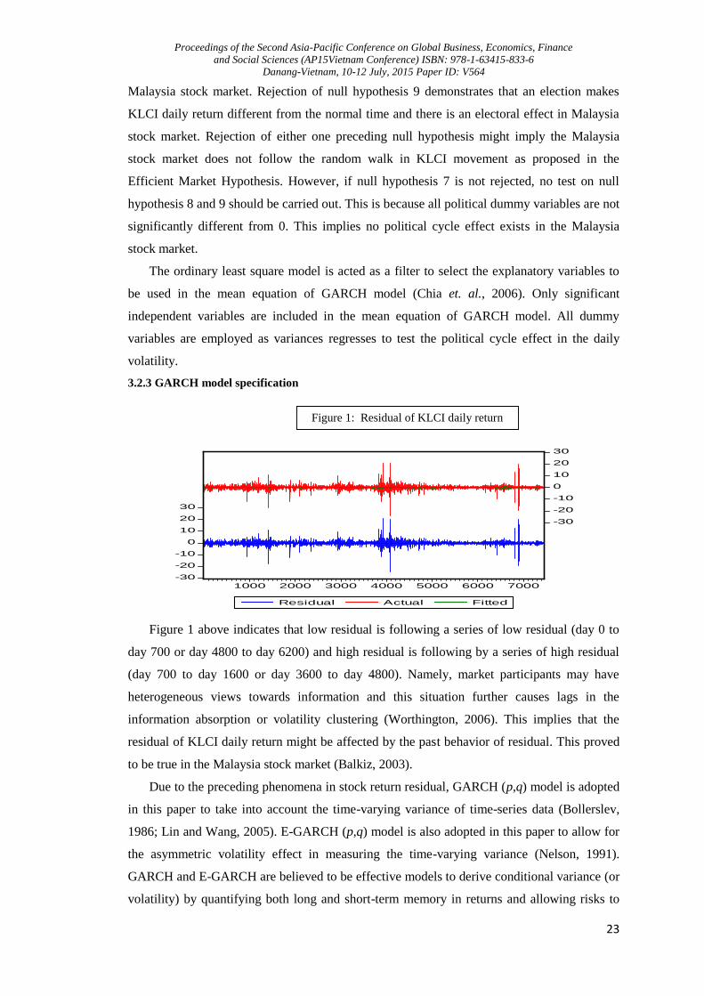
Figure 1 above indicates that low residual is following a series of low residual (day 0 to
day 700 or day 4800 to day 6200) and high residual is following by a series of high residual
(day 700 to day 1600 or day 3600 to day 4800). Namely, market participants may have
heterogeneous views towards information and this situation further causes lags in the
information absorption or volatility clustering (Worthington, 2006). This implies that the
residual of KLCI daily return might be affected by the past behavior of residual. This proved
to be true in the Malaysia stock market (Balkiz, 2003).
Due to the preceding phenomena in stock return residual, GARCH (p,q) model is adopted
in this paper to take into account the time-varying variance of time-series data (Bollerslev,
1986; Lin and Wang, 2005). E-GARCH (p,q) model is also adopted in this paper to allow for
the asymmetric volatility effect in measuring the time-varying variance (Nelson, 1991).
GARCH and E-GARCH are believed to be effective models to derive conditional variance (or
volatility) by quantifying both long and short-term memory in returns and allowing risks to
-30
-20
-10
0
10
20
30
-30
-20
-10
0
10
20
30
1000 2000 3000 4000 5000 6000 7000
Residual Actual Fitted
Figure 1: Residual of KLCI daily return
Proceedings of the Second Asia-Pacific Conference on Global Business, Economics, Finance
and Social Sciences (AP15Vietnam Conference) ISBN: 978-1-63415-833-6
Danang-Vietnam, 10-12 July, 2015 Paper ID: V564
24
vary over time (Bollerslev, 1986; Engle and Ng, 1993; Leblang and Mukherjee, 2003;
Beaulieu, 2005; Worthington, 2006; Wong and McAleer, 2009).
Ljung-Box 𝑄2 test and Lagrange Multiplier test (Engle, 1982) for first 6 and 12 lags are
applied to justify the use of ARCH-type models for the variance by accounting for the level of
serial correlation in the daily return series. Further, sign bias test, negative size bias test,
positive sign bias test and joint test proposed by Engle and Ng (1993) are applied in the
diagnostics to investigate whether shocks on the KLCI return have an asymmetric effect on
the volatility and whether E-GARCH is applicable to model the volatility. Sign bias test is
used to address the impact of positive and negative innovation on volatility not predicted by
the model. Negative size bias test is used to capture the impact of large and small negative
innovations on volatility. Positive size bias test is used to examine possible biases associated
with large and small positive innovations. Joint test simultaneously considers preceding three
tests to test the linear ARCH or GARCH against the asymmetry (Engle and Ng, 1993;
Hagerud, 1997; Henry and Suardi, 2005; Brandt and Jones, 2006; Koulakoitis et. al., 2008).
The GARCH (p,q) model and E-GARCH (p,q) model in this paper are adapted from the
researches of Leblang and Murkherjee (2005), Li and Born (2006), Worthington (2006),
Beaulieu et. al. (2006), Siokis and Kapopoulos (2007) Koulakiotis et. al. (2008), in which
these researches are measuring the relationship between electoral or political factors and stock
market volatility. GARCH (p,q) is used to capture the symmetric response to news or shocks
whereas E-GARCH (p,q) is used to capture the volatility effect.
The GARCH (p,q) model is described as follow:
Rt = α0 + αl ∑ 𝑧l𝑚𝑙=1 + γo ht + εt (1)
htg = τ0 + βi ∑ 𝜀2𝑡 − 𝑖𝑝𝑖=1 + γj ∑ h𝑡 − 𝑗
𝑞𝑗=1 + τk ∑ 𝑥𝑘𝑛
𝑘=1 (2)
εt Ωt-1 ~ N ( 0, htg ) (3)
Where the variables in the mean equation (1) are as follows:
Rt = Market return at time t.
α0 = Intercept
zl = The set of l control variables to Rt (where l = GDPt and USt).
Xk = the set of k political factors expected to influence Rt (where x = Mt, Nt, Qt, Bt, At and Tt).
ht = Daily volatility of the daily return derived from GARCH at time t.
εt = Error term.
τk = Coefficient of political dummy variables to the volatility.
βi = Coefficient of the previous day’s noise.
γj = Coefficient of the previous day’s volatility.
The E-GARCH (p,q) model is described as follow (using mean equation 1 as well):

Proceedings of the Second Asia-Pacific Conference on Global Business, Economics, Finance
and Social Sciences (AP15Vietnam Conference) ISBN: 978-1-63415-833-6
Danang-Vietnam, 10-12 July, 2015 Paper ID: V564
25
hte = τ0 + βi {∑ [𝑢𝑡 − 𝑖 − 𝐸 𝑢𝑡 − 𝑖 + 𝜃𝑢𝑡 − 𝑖]𝑝𝑖=1 }+ γj ln [∑ h𝑡 − 𝑗
𝑞𝑗=1 ] + τk ∑ 𝑥𝑘𝑛
𝑘=1 (4)
εt Ωt-1 ~ N ( 0, hts ) (5)
hte = Daily volatility of the daily return derived from E-GARCH at time t.
θ = Coefficient to capture the impact of noise.
Lag interval is determined by the Schwart information criteria (SIC) as it is more
consistent than the Akaike information criteria since it penalizes most heavily the degree of
freedom (Schwars, 1978; Lutkepohl, 1991; as cited in Chia, 2006). The highest order
considered in this paper is 5 for p and q. Various combinations of p and q are tested within the
range from 1 to 5 in both cases to select the best fit GARCH (p,q) model. The combination of
orders that produces the minimum SIC with p-value lower than 0.05 will be chosen. When the
Jarque-Bera test indicates that there is significant kurtosis in the data, Bollerslev and
Wooldridge (1992) semi-robust standard errors are applied to provide unbiased standard
errors that are robust to deviation in normality of the residuals.
Diagnostic tests of both models consist of Ljung-Box 𝑄2 test and ARCH-Lagrange
Multiplier. These two tests examine whether ARCH effect remains in the variance derived by
both GARCH models. If the leverage effect (θ) is not significant in the E-GARCH model, the
result from GARCH model will be adopted to draw the conclusion.
Null hypothesis 10 test whether electoral and political factors affect the daily return or of
KLCI:
10) H0: τ1 = τ2 = τ3 = τ4 = τ5 = 0
When some τ ≠ 0, the null hypothesis 10 is rejected. It indicates that market volatility exhibits
the pattern of election cycle and the electoral and political factors do impact the daily return
of KLCI. If the null hypothesis 10 is rejected, the hypothesis 11 and the hypothesis 12 are
tested.
The null hypothesis 11 tests whether different Prime Minister Regimes post different level of
impact to the variance of market volatility:
11) H0: τ1 = τ2 = τ3
The null hypothesis 12 tests whether the election posts different impacts to the pre-election
and post-election variance of market volatility:
12) H0: τ 4 = τ 5
Null hypothesis 10, 11 and12 are adopted from hypothesis 7, 8 and 9. Hence, the explanation
for rejection of null hypothesis is same, except null hypothesis 7, 8 and 9 are used to draw the
impacts of political dummy variables towards the return whereas null hypothesis 10, 11 and12
are for volatility aspect. Results of null hypotheses tests are shown in the chapter 4. Possible
reasons to result in the rejection or non-rejection of null hypothesis are discussed in the
chapter 4 as well.
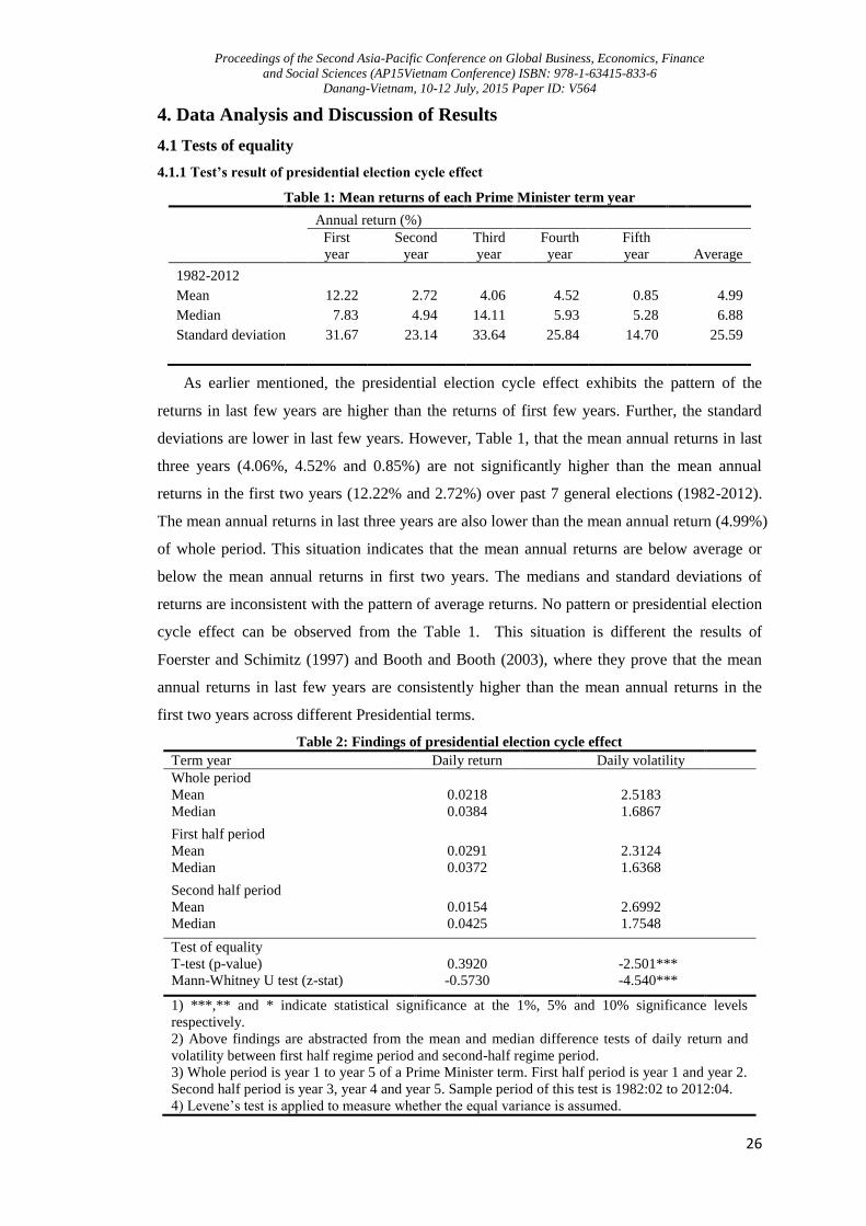
Proceedings of the Second Asia-Pacific Conference on Global Business, Economics, Finance
and Social Sciences (AP15Vietnam Conference) ISBN: 978-1-63415-833-6
Danang-Vietnam, 10-12 July, 2015 Paper ID: V564
26
4. Data Analysis and Discussion of Results
4.1 Tests of equality
4.1.1 Test’s result of presidential election cycle effect
Table 1: Mean returns of each Prime Minister term year
Annual return (%)
First
year
Second
year
Third
year
Fourth
year
Fifth
year
Average
1982-2012
Mean 12.22
2.72
4.06
4.52
0.85
4.99
Median 7.83
4.94
14.11
5.93
5.28
6.88
Standard deviation 31.67
23.14
33.64
25.84
14.70
25.59
As earlier mentioned, the presidential election cycle effect exhibits the pattern of the
returns in last few years are higher than the returns of first few years. Further, the standard
deviations are lower in last few years. However, Table 1, that the mean annual returns in last
three years (4.06%, 4.52% and 0.85%) are not significantly higher than the mean annual
returns in the first two years (12.22% and 2.72%) over past 7 general elections (1982-2012).
The mean annual returns in last three years are also lower than the mean annual return (4.99%)
of whole period. This situation indicates that the mean annual returns are below average or
below the mean annual returns in first two years. The medians and standard deviations of
returns are inconsistent with the pattern of average returns. No pattern or presidential election
cycle effect can be observed from the Table 1. This situation is different the results of
Foerster and Schimitz (1997) and Booth and Booth (2003), where they prove that the mean
annual returns in last few years are consistently higher than the mean annual returns in the
first two years across different Presidential terms.
Table 2: Findings of presidential election cycle effect
Term year Daily return Daily volatility
Whole period
Mean
0.0218
2.5183
Median
0.0384
1.6867
First half period
Mean
0.0291
2.3124
Median
0.0372
1.6368
Second half period
Mean
0.0154
2.6992
Median
0.0425
1.7548
Test of equality
T-test (p-value)
0.3920
-2.501***
Mann-Whitney U test (z-stat)
-0.5730
-4.540***
1) ***,** and * indicate statistical significance at the 1%, 5% and 10% significance levels
respectively.
2) Above findings are abstracted from the mean and median difference tests of daily return and
volatility between first half regime period and second-half regime period.
3) Whole period is year 1 to year 5 of a Prime Minister term. First half period is year 1 and year 2.
Second half period is year 3, year 4 and year 5. Sample period of this test is 1982:02 to 2012:04.
4) Levene’s test is applied to measure whether the equal variance is assumed.
Proceedings of the Second Asia-Pacific Conference on Global Business, Economics, Finance
and Social Sciences (AP15Vietnam Conference) ISBN: 978-1-63415-833-6
Danang-Vietnam, 10-12 July, 2015 Paper ID: V564
27
5) Null hypothesis 1 - Mean daily returns do not differ between the first half regime period and the
second half regime period.
6) Null hypothesis 2 - Mean daily volatilities do not differ between the first half regime period and
the second half regime period.
The presidential election cycle effect is further documented in the table 2 to statistically
test the presence of mean and median difference between the first half period and second half
period. Namely, the mean daily returns and volatility and median daily return and volatility in
the first half period (first two years) are compared against the second half period (last three
years) in the t-test and Mann-Whitney U test respectively. By observing the mean in the first
and second half period, it clearly shows that the mean daily return in the second half period is
lower than the first half period whereas the mean daily volatility in the second half period is
higher than the first half period.
Both t-test and Mann-Whitney U test do not find any statistically significant difference in
daily returns between the first half period and the second half period. Namely, the difference
in daily returns between two periods over the past 7 general elections is not significant even at
the 0.1 significance level. Hence, the null hypothesis 1 regarding the difference in daily
returns between the two periods is not rejected. In contrast, both t-test and Mann-Whitney U
test provide strong evidences to reject the null hypothesis 2. The mean difference and median
difference in daily volatilities between the two periods are significant at the 0.01 significance
level. This result shows that the mean daily volatilities of second half periods have been
statistically higher than first half periods over the past 7 general elections. Namely, the
Malaysia stock market is more volatile during the second half regime period of a Prime
Minister term.
For a presidential election cycle effect to be proven in a stock market, daily returns (daily
volatilities) in the second half regime period must be higher (lower) than the first half regime
period. However, the results of table 2 clearly show that the difference in daily returns
between two periods is not significant. Further, the daily volatilities in the second regime half
period are significantly higher than the first half regime period. Hence, the findings in table 2
are different from studies by Huang (1985), Stovall (1992), Gartner and Wellershoff (1995),
Foerster and Schimitz (1997), Banning and Jones (2002), Booth and Booth (2003), Swenden
and Patel (2004) and Kraussl et. al. (2008). Therefore, based on the findings, the Malaysia
stock market does not exhibit the behavior of presidential election cycle. However, the
significant mean difference in daily volatilities between first half period and second half
period should be noticed because it does show that the Prime Minister term does impact the
level of volatility.
Although Alt and Lassen (2006) find that the presidential election cycle usually takes
place in low fiscal balance transparency countries, this effect is not observable in the
Malaysia stock market. This result may indicate that a Prime Minister may not manipulate the
Proceedings of the Second Asia-Pacific Conference on Global Business, Economics, Finance
and Social Sciences (AP15Vietnam Conference) ISBN: 978-1-63415-833-6
Danang-Vietnam, 10-12 July, 2015 Paper ID: V564
28
fiscal or monetary policy to increase the possibility of winning in the coming general
elections. Incapability of exercising effective policies or implemented policies do not fully
absorb by the public could also contribute to this result. For example, the effectiveness of
social-benefiting policy might be impaired by the corruption. High confidence of winning in
the next general election might also slacken the incumbent party to manipulate the fiscal or
monetary of policy. Less possibly, the incumbent party is not interested to seek re-election in
the next general election.
4.1.2 Test’s result of Prime Minister Effect
Table 3: Findings of Prime Minister Effect
Regime In-government Out-of government
Tests of equality of
means
Mean
Mean
t-stat
Days Return Volatility Days Return Volatility Return Volatility
Mahathir
5378 0.0194 2.8480
2003 0.0282 1.6330
-0.253 7.0190***
Abdullah
984 0.0366 0.5621
6397 0.0195 2.8192
0.542 -22.092***
Najib
1019 0.0202 2.6672
6362 0.0221 2.4944
-0.037 0.6620
1) ***, ** and * indicate statistical significance at the 1%, 5% and 10% significance levels respectively.
2) Above findings are abstracted from the mean difference test of return and volatility between in-government
regime and out-of government regime under different Prime Ministers.
3) Regime refers to the name of Prime Minister. Days refer to the number of trading days. Return and
volatility under the “Mean” particular are presented on a mean daily basis. Return and volatility under the “t-
stat” particular are the t-stat of return and volatility retrieved from the t-test. Sample period of this test is
1982:02 to 2012:04.
4) Levene’s test is applied to measure whether the equal variance is assumed.
5) Null hypothesis 3 - Mean daily returns do not differ across different Prime Ministers.
6) Null hypothesis 4 - Mean daily volatilities do not differ across different Prime Ministers.
The Table 3 shows both descriptive statistics of mean daily return and means daily
volatilities under different Prime Minister Regimes. Mahathir holds the longest period in the
office by being a Prime Minister over 5378 trading days. Abdullah’s regime holds the highest
daily return (0.0366%) and the lowest daily volatility (0.5621%). The stock market
performance under the Abdullah’s regime outperforms the other regimes. Stock market
performances under Mahathir’s regime and Najib’s regime are similar. Both of their regimes
underperform against the other regimes. This result subtly implies that Abdullah’s political
policy is more beneficial than the other Prime Minister to the stock market, in terms of better
return and stability. Global economic booming during the Prime Minister term of Abdullah
could be another reason to explain his superior performance.
However, empirically, the mean daily returns do not differ across different Prime
Ministers by referring to the t-stats of mean daily return in the Table 3 The findings show
there is no significant mean difference in daily returns between a regime and other regimes.
This result is different from the above conclusion based on the descriptive statistics. In
contrast, based on the findings, it shows that there is significant mean difference in daily
volatilities between a regime and other regimes. Hence, the null hypothesis 3 is not rejected
Proceedings of the Second Asia-Pacific Conference on Global Business, Economics, Finance
and Social Sciences (AP15Vietnam Conference) ISBN: 978-1-63415-833-6
Danang-Vietnam, 10-12 July, 2015 Paper ID: V564
29
since the mean daily returns do not differ across different Prime Ministers. This result is
consistent with the findings of Worthington (2006).
In contrast, under regimes of Mahathir and Abdullah, the mean difference in daily
volatilities between their in-government time and out-of government time is significant at the
0.01 significance level. This indicates that different Prime Ministers bring dissimilar impacts
to the stock market fluctuation. For example, Abdullah brings significantly less turbulence to
the stock market than the other Prime Ministers. This result could be related to the
characteristics of a Prime Minister as more aggressive Prime Minister might bring higher
volatilities to the stock market, vice versa. Different policy orientation between Prime
Ministers unlike economic conditions could be factors contributing to this significance as well.
Table 4: Findings of Prime Minister effect around general election
Regime Before one week After one week
Tests of equality of
means (t-stat)
Return Volatility Return Volatility Return Volatility
Whole period
0.1475 1.1976
-0.2410 1.6191
0.9270 -2.605***
Mahathir
0.3017 1.1917
0.0301 1.3417
0.7890 -1.941*
Abdullah
0.4449 1.0063
-0.2074 0.9583
1.4730 -0.022
Najib
-0.9201 1.4181
-1.6310 3.6667
0.2950 -3.828***
Regime Before one month After one month
Tests of equality of
means
Return Volatility Return Volatility Return Volatility
Whole period
-0.0151 1.3157
0.0893 1.4263
-0.6350 -2.767***
Mahathir
0.0151 1.3909
0.2332 1.3424
1.0680 -0.005
Abdullah
0.2598 1.1199
-0.2415 0.8747
2.059** 1.580
Najib
-0.4413 1.1357
-0.2990 2.3979
-0.2250 -4.624***
1) ***, ** and * indicate statistical significance at the 1%, 5% and 10% significance levels respectively.
2) Above findings are abstracted from the mean difference test of return and volatility between pre-election period
and post-election period under different Prime Ministers.
3) Regime refers to the name of Prime Minister. Whole period refers to the whole sample period from 1982:02 to
2012:04.
4) Levene’s test is applied to measure whether the equal variance is assumed.
The findings of Prime Minister Effect are further expanded in the Table 4 by testing the
mean difference in return and volatility between pre-election period and post-election period.
By observing the t-stat in daily returns between pre-election period and post-election period,
only one month before and one month after Abdullah’s election has significant mean
difference at the significance level of 0.05. Apart from that, no significance is found in the
whole period, Mahathir’s regime and Abdullah’s regime. This result is consistent with the
findings of Table 3 as the Prime Minister effect is not found on the ground of daily returns.
The mean difference in return is not significant may be contributed by the poor policy of
effectively allocating country resources. Since all Prime Ministers are coming from the same

Proceedings of the Second Asia-Pacific Conference on Global Business, Economics, Finance
and Social Sciences (AP15Vietnam Conference) ISBN: 978-1-63415-833-6
Danang-Vietnam, 10-12 July, 2015 Paper ID: V564
30
party, the market might not perceive more benefits or deteriorations even the Prime Minister
is changed. Hence, the mean difference in daily return is insignificant.
Further, the findings for mean difference in daily volatilities between pre-election period
and post-election period are slightly different the result of Table 3 Refer to the Table 4, in
one-month period, the mean difference in daily volatility is significant at the 0.01significance
level in both whole period comparison and Najib’s regime. In one-week period, the mean
difference in daily volatility is significant at the 0.1 significance level in the Mahathir’s
regime and at the 0.01 significance level in both whole period comparison and Najib’s regime.
The volatility of post-election period is significantly higher than the pre-election period under
the elections of Najib’s party, as well the average of all elections (whole period).
Aforementioned, there is a persistently significant incongruence between the vote percentage
and seat percentage across all past general elections. This might indicate that investors carry
out a series of post-election portfolio adjustment to rectify their pre-election expectation, as
suggest by He et. al. (2009).
The post-election daily volatility is significantly higher than the pre-election condition
under the Najib’s regime is expected. This is because the public posts distrust to the
Abdullah’s administration and a very early election was held in year 4 (Usually in year 5) of
Abdullah’s Prime Minister Term to replace Abdullah. The Barisan Nasional experienced the
unprecedented greatest losses in Parliament seats during the 2008 election. A mismatch
between investors’ pre-election expectation and actual result causes investors adjusting their
portfolio drastically. Hence, the post-election daily volatility is significantly higher than the
pre-election condition under the Najib’s regime.
Conclusively, the null hypothesis 3 is not rejected and the Prime Minister effect is
insignificant in the mean daily return. There is no conclusion for the null hypothesis 4 since
there are a number of significant mean differences in both Table 3 and Table 4. However, it
only implies a mediocre presence of the Prime Minister effect in the KLCI daily volatility.
4.1.3 Test’s result of electoral effect
Table 5: Findings of electoral effect
Window Mean difference (t-test) Z-stat ( Mann-Whitney U test)
Return Volatility Return Volatility
Panel A: Symmetric event windows
(-1,1) -0.1506 0.3145
-0.274 -0.396
(-2,2) 0.2091 0.5142
-1.845* -0.103
(-5,5) -0.0778 0.3332
-0.002 -0.441
(-10,10) 0.0117 0.1901
-0.278 -0.027
(-20,20) -0.0029 0.1038
-0.336 -1.109
Panel B: Asymmetric event windows
(-20,0) -0.0434 -0.2333*
-0.564 -0.020
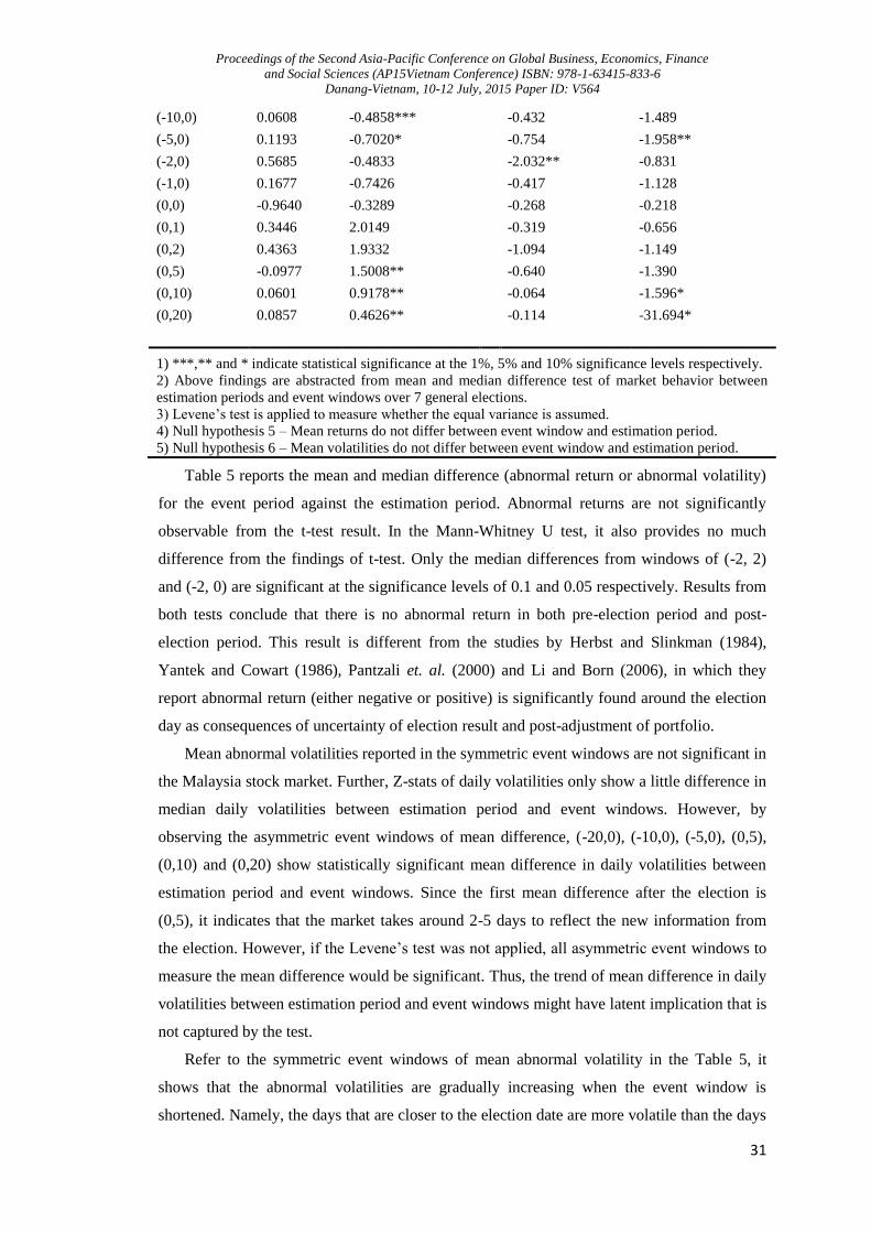
Proceedings of the Second Asia-Pacific Conference on Global Business, Economics, Finance
and Social Sciences (AP15Vietnam Conference) ISBN: 978-1-63415-833-6
Danang-Vietnam, 10-12 July, 2015 Paper ID: V564
31
(-10,0) 0.0608 -0.4858***
-0.432 -1.489
(-5,0) 0.1193 -0.7020*
-0.754 -1.958**
(-2,0) 0.5685 -0.4833
-2.032** -0.831
(-1,0) 0.1677 -0.7426
-0.417 -1.128
(0,0) -0.9640 -0.3289
-0.268 -0.218
(0,1) 0.3446 2.0149
-0.319 -0.656
(0,2) 0.4363 1.9332
-1.094 -1.149
(0,5) -0.0977 1.5008**
-0.640 -1.390
(0,10) 0.0601 0.9178**
-0.064 -1.596*
(0,20) 0.0857 0.4626**
-0.114 -31.694*
1) ***,** and * indicate statistical significance at the 1%, 5% and 10% significance levels respectively.
2) Above findings are abstracted from mean and median difference test of market behavior between
estimation periods and event windows over 7 general elections.
3) Levene’s test is applied to measure whether the equal variance is assumed.
4) Null hypothesis 5 – Mean returns do not differ between event window and estimation period.
5) Null hypothesis 6 – Mean volatilities do not differ between event window and estimation period.
Table 5 reports the mean and median difference (abnormal return or abnormal volatility)
for the event period against the estimation period. Abnormal returns are not significantly
observable from the t-test result. In the Mann-Whitney U test, it also provides no much
difference from the findings of t-test. Only the median differences from windows of (-2, 2)
and (-2, 0) are significant at the significance levels of 0.1 and 0.05 respectively. Results from
both tests conclude that there is no abnormal return in both pre-election period and post-
election period. This result is different from the studies by Herbst and Slinkman (1984),
Yantek and Cowart (1986), Pantzali et. al. (2000) and Li and Born (2006), in which they
report abnormal return (either negative or positive) is significantly found around the election
day as consequences of uncertainty of election result and post-adjustment of portfolio.
Mean abnormal volatilities reported in the symmetric event windows are not significant in
the Malaysia stock market. Further, Z-stats of daily volatilities only show a little difference in
median daily volatilities between estimation period and event windows. However, by
observing the asymmetric event windows of mean difference, (-20,0), (-10,0), (-5,0), (0,5),
(0,10) and (0,20) show statistically significant mean difference in daily volatilities between
estimation period and event windows. Since the first mean difference after the election is
(0,5), it indicates that the market takes around 2-5 days to reflect the new information from
the election. However, if the Levene’s test was not applied, all asymmetric event windows to
measure the mean difference would be significant. Thus, the trend of mean difference in daily
volatilities between estimation period and event windows might have latent implication that is
not captured by the test.
Refer to the symmetric event windows of mean abnormal volatility in the Table 5, it
shows that the abnormal volatilities are gradually increasing when the event window is
shortened. Namely, the days that are closer to the election date are more volatile than the days
Proceedings of the Second Asia-Pacific Conference on Global Business, Economics, Finance
and Social Sciences (AP15Vietnam Conference) ISBN: 978-1-63415-833-6
Danang-Vietnam, 10-12 July, 2015 Paper ID: V564
32
that are farther to the election date. By further observing the asymmetric event windows of
mean abnormal volatility, it suggests that there is observer or waiting behavior before the
election as pre-election mean abnormal volatilities are negative. After the election result is
publicly known, the post-election portfolio adjustment trigger an extremely high volatility on
(0, 1) and the volatility gradually decreases when the day is farther to the election date. This is
because the information has been gradually incorporating in the stock market sentiment. The
post-election volatilities are usual as the new government might bring new political landscape
to the market or the election result is unexpected by major investors (Ploeg, 1989; He et. al.,
2009).
Conclusively, the null hypothesis 5 is not rejected. Namely, the electoral effect is not
observable in the behavior of stock market return. However, the null hypothesis 6 is rejected
since the moving tendency of KLCI daily volatility is observable and half amount of total
event windows do show significance in mean between estimation period and event windows.
Hence, the electoral effect does present in the variance of daily volatility of Malaysia stock
market.
Based on preceding three tests of equality, it shows that there is mediocre relationship
between the political cycle effect and KLCI daily volatility because it is observable in the
stock market volatility in the tests of presidential cycle, Prime Minister Effect and electoral
effect. Nevertheless, the behavior of KLCI daily return does not exhibit the political cycle
effect. Risk and return tradeoff is violated due to the incongruence in political cycle effect
between return and volatility. Although the findings for the behavior of return and volatility
are inconsistent, investors still need to pay attention to the change in the political factors since
the political cycle effects are empirically proved by the other researchers. Especially, the non-
value-added additional volatility presents in the stock market in this section.
Two further analyses are carried to confirm the findings from the equality tests. First, an
ordinary least square regression analysis is adopted in the section 4.2 to confirm the findings
of the behavior of stock market return. Second, GARCH models are adopted in the section 4.3
to confirm the findings of the behavior of stock market return. These tests also provide the
magnitude of each dummy variable to the estimation of return and volatility. Hence, the
factors and individual impacts of causing the political cycle can be observed sophisticatedly.
4.2 Regression model specification for KLCI daily return
4.2.1 Descriptive statistics
Table 6: Descriptive statistics of time-series variables
KLCI daily return NYSE daily return GDP
Mean 0.0202
0.0246 0.0229
Standard deviation 1.5007
1.1145 0.0516
Skewness -0.2196
-1.3109 -1.2940
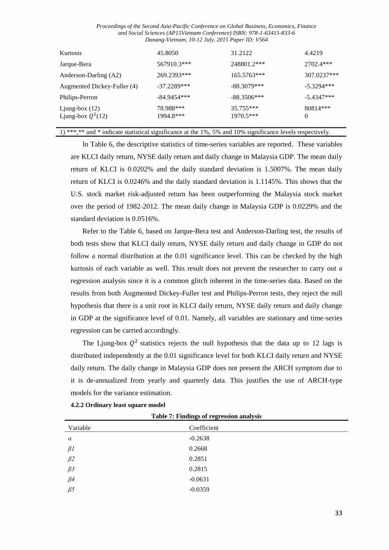
Proceedings of the Second Asia-Pacific Conference on Global Business, Economics, Finance
and Social Sciences (AP15Vietnam Conference) ISBN: 978-1-63415-833-6
Danang-Vietnam, 10-12 July, 2015 Paper ID: V564
33
Kurtosis 45.8050
31.2122 4.4219
Jarque-Bera 567910.3***
248801.2*** 2702.4***
Anderson-Darling (A2) 269.2393***
165.5763*** 307.0237***
Augmented Dickey-Fuller (4) -37.2289***
-88.3079*** -5.3294***
Philips-Perron -84.9454***
-88.3506*** -5.4347***
Ljung-box (12) 78.988***
35.755*** 80814***
Ljung-box 𝑄2(12)
1994.8***
1970.5***
0
1) ***,** and * indicate statistical significance at the 1%, 5% and 10% significance levels respectively.
In Table 6, the descriptive statistics of time-series variables are reported. These variables
are KLCI daily return, NYSE daily return and daily change in Malaysia GDP. The mean daily
return of KLCI is 0.0202% and the daily standard deviation is 1.5007%. The mean daily
return of KLCI is 0.0246% and the daily standard deviation is 1.1145%. This shows that the
U.S. stock market risk-adjusted return has been outperforming the Malaysia stock market
over the period of 1982-2012. The mean daily change in Malaysia GDP is 0.0229% and the
standard deviation is 0.0516%.
Refer to the Table 6, based on Jarque-Bera test and Anderson-Darling test, the results of
both tests show that KLCI daily return, NYSE daily return and daily change in GDP do not
follow a normal distribution at the 0.01 significance level. This can be checked by the high
kurtosis of each variable as well. This result does not prevent the researcher to carry out a
regression analysis since it is a common glitch inherent in the time-series data. Based on the
results from both Augmented Dickey-Fuller test and Philips-Perron tests, they reject the null
hypothesis that there is a unit root in KLCI daily return, NYSE daily return and daily change
in GDP at the significance level of 0.01. Namely, all variables are stationary and time-series
regression can be carried accordingly.
The Ljung-box 𝑄2 statistics rejects the null hypothesis that the data up to 12 lags is
distributed independently at the 0.01 significance level for both KLCI daily return and NYSE
daily return. The daily change in Malaysia GDP does not present the ARCH symptom due to
it is de-annualized from yearly and quarterly data. This justifies the use of ARCH-type
models for the variance estimation.
4.2.2 Ordinary least square model
Table 7: Findings of regression analysis
Variable Coefficient
α -0.2638
β1 0.2668
β2 0.2851
β3 0.2815
β4 -0.0631
β5 -0.0359
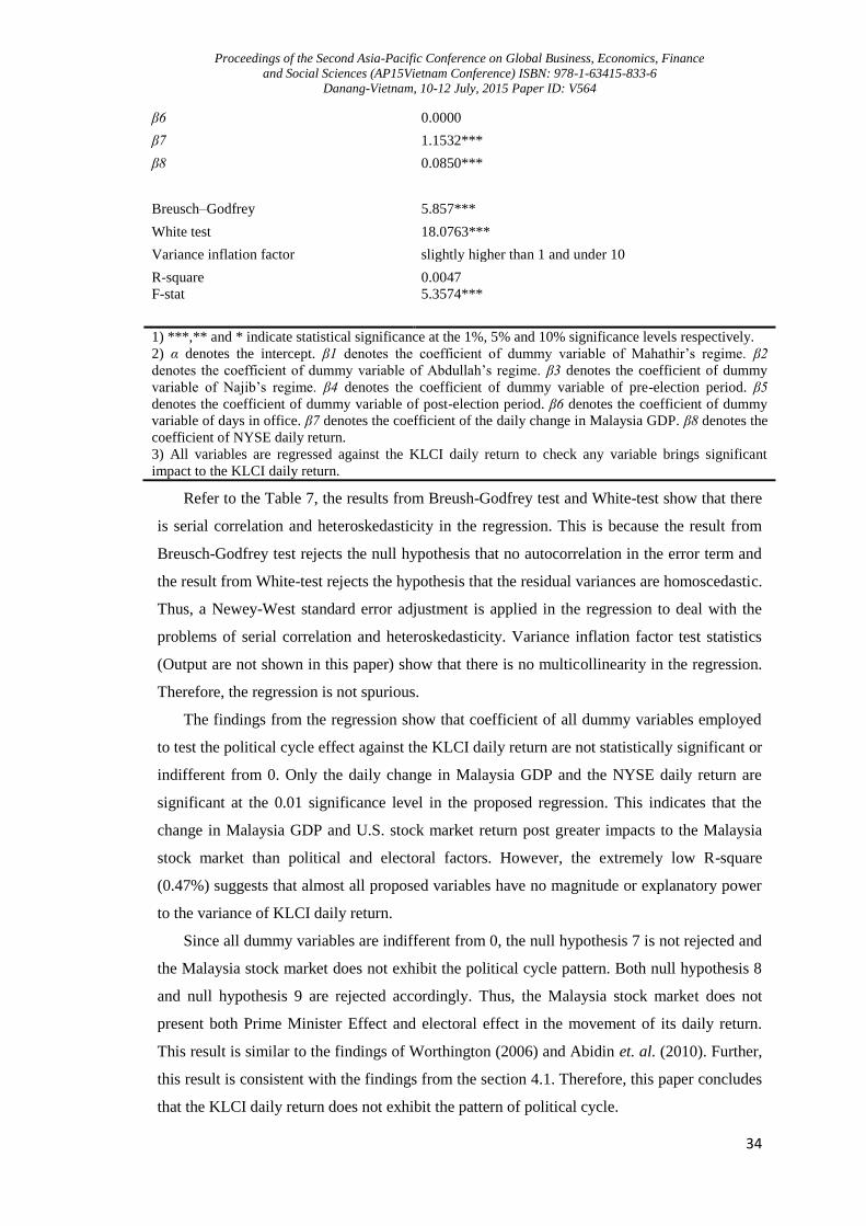
Proceedings of the Second Asia-Pacific Conference on Global Business, Economics, Finance
and Social Sciences (AP15Vietnam Conference) ISBN: 978-1-63415-833-6
Danang-Vietnam, 10-12 July, 2015 Paper ID: V564
34
β6 0.0000
β7 1.1532***
β8 0.0850***
Breusch–Godfrey 5.857***
White test 18.0763***
Variance inflation factor slightly higher than 1 and under 10
R-square 0.0047
F-stat 5.3574***
1) ***,** and * indicate statistical significance at the 1%, 5% and 10% significance levels respectively.
2) α denotes the intercept. β1 denotes the coefficient of dummy variable of Mahathir’s regime. β2
denotes the coefficient of dummy variable of Abdullah’s regime. β3 denotes the coefficient of dummy
variable of Najib’s regime. β4 denotes the coefficient of dummy variable of pre-election period. β5
denotes the coefficient of dummy variable of post-election period. β6 denotes the coefficient of dummy
variable of days in office. β7 denotes the coefficient of the daily change in Malaysia GDP. β8 denotes the
coefficient of NYSE daily return.
3) All variables are regressed against the KLCI daily return to check any variable brings significant
impact to the KLCI daily return.
Refer to the Table 7, the results from Breush-Godfrey test and White-test show that there
is serial correlation and heteroskedasticity in the regression. This is because the result from
Breusch-Godfrey test rejects the null hypothesis that no autocorrelation in the error term and
the result from White-test rejects the hypothesis that the residual variances are homoscedastic.
Thus, a Newey-West standard error adjustment is applied in the regression to deal with the
problems of serial correlation and heteroskedasticity. Variance inflation factor test statistics
(Output are not shown in this paper) show that there is no multicollinearity in the regression.
Therefore, the regression is not spurious.
The findings from the regression show that coefficient of all dummy variables employed
to test the political cycle effect against the KLCI daily return are not statistically significant or
indifferent from 0. Only the daily change in Malaysia GDP and the NYSE daily return are
significant at the 0.01 significance level in the proposed regression. This indicates that the
change in Malaysia GDP and U.S. stock market return post greater impacts to the Malaysia
stock market than political and electoral factors. However, the extremely low R-square
(0.47%) suggests that almost all proposed variables have no magnitude or explanatory power
to the variance of KLCI daily return.
Since all dummy variables are indifferent from 0, the null hypothesis 7 is not rejected and
the Malaysia stock market does not exhibit the political cycle pattern. Both null hypothesis 8
and null hypothesis 9 are rejected accordingly. Thus, the Malaysia stock market does not
present both Prime Minister Effect and electoral effect in the movement of its daily return.
This result is similar to the findings of Worthington (2006) and Abidin et. al. (2010). Further,
this result is consistent with the findings from the section 4.1. Therefore, this paper concludes
that the KLCI daily return does not exhibit the pattern of political cycle.

Proceedings of the Second Asia-Pacific Conference on Global Business, Economics, Finance
and Social Sciences (AP15Vietnam Conference) ISBN: 978-1-63415-833-6
Danang-Vietnam, 10-12 July, 2015 Paper ID: V564
35
Since all dummy variables are insignificant, only the daily change in Malaysia GDP and
the NYSE daily return are used as explanatory variables of the mean equation of GARCH
model. However, all dummy variables are still employed as variance regressors to test the
impact of each dummy variable to the fluctuation of Malaysia stock market.
4.3 GARCH model specification
Table 8: Findings of indicators to carry out a GARCH model
Sign bias 0.04463
Negative size bias test -4.3058***
Positive size bias test 3.57***
Joint test 468.0521***
ARCH-LM (6)
ARCH-LM (12)
426.8022***
214.6454***
Ljung-box 𝑄2 (6) 2704.3***
Ljung-box 𝑄2 (12) 2805.5***
White test
43.0618***
1) *** indicate statistical significance at the 1% significance level.
2) These tests examine whether the shocks on KLCI daily return
have an asymmetric effect on volatility.
Table8 signify a need to carry out a GARCH model on modeling the daily variance. First,
negative size bias test, positive size bias test and joint test are significant at the 0.01
significance level. This indicates asymmetries are presented in the conditional variance.
Second, both Ljung-box 𝑄2statistics and ARCH Lagrange Multiplier are significant at the
0.01 significance level. They signify that there is remaining ARCH effect or past innovation
in the KLCI volatility and an ARCH type model should be adopted to sophisticatedly explain
the variance. Last, the residual of KLCI daily return model is detected as conditionally
heteroskedastic by referring to the White heteroskedasticity test statistics.
These findings suggest that the volatility specification should include components of
conditional heteroskedasticity and asymmetry to adequately model the KLCI volatility as the
shock of KLCI daily returns have an asymmetric effect on volatility. Hence, both GARCH
(p,q) and E-GARCH (p,q) are adopted in this paper to derive the conditional volatility. Both
models are estimated with Bollerslev and Wooldridge semi-robust standard errors as the
Jarque-Bera test indicates that kurtosis presents in variables.
Table 8.1: Findings of GARCH (p,q) order
ARCH (p)
Order 1 2 3 4 5
GARCH (q) 1 3.1039 3.1030 3.1032 3.1103 3.1046
2 3.1036 3.1042 3.1046 3.1048 3.1047
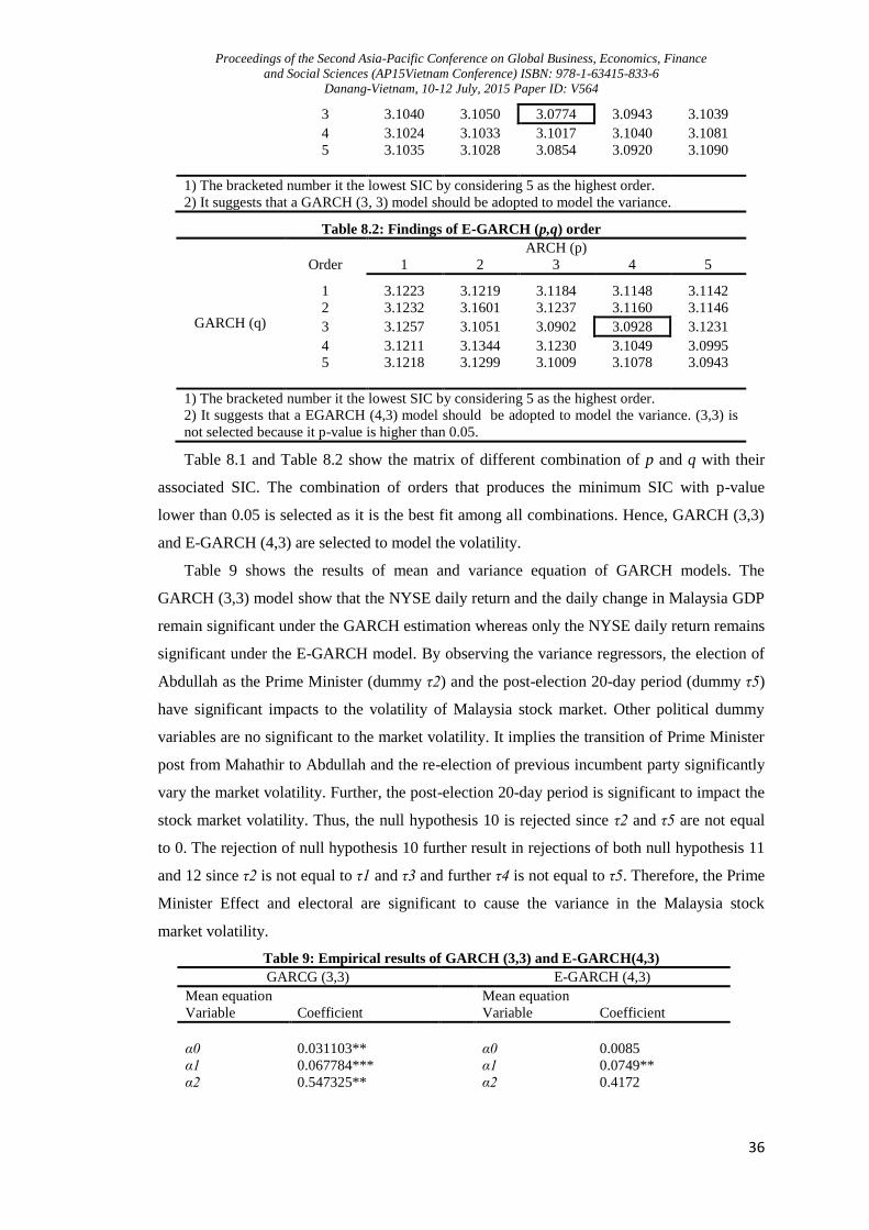
Proceedings of the Second Asia-Pacific Conference on Global Business, Economics, Finance
and Social Sciences (AP15Vietnam Conference) ISBN: 978-1-63415-833-6
Danang-Vietnam, 10-12 July, 2015 Paper ID: V564
36
3 3.1040 3.1050 3.0774 3.0943 3.1039
4 3.1024 3.1033 3.1017 3.1040 3.1081
5 3.1035 3.1028 3.0854 3.0920 3.1090
1) The bracketed number it the lowest SIC by considering 5 as the highest order.
2) It suggests that a GARCH (3, 3) model should be adopted to model the variance.
Table 8.2: Findings of E-GARCH (p,q) order
ARCH (p)
Order 1 2 3 4 5
GARCH (q)
1 3.1223 3.1219 3.1184 3.1148 3.1142
2 3.1232 3.1601 3.1237 3.1160 3.1146
3 3.1257 3.1051 3.0902 3.0928 3.1231
4 3.1211 3.1344 3.1230 3.1049 3.0995
5 3.1218 3.1299 3.1009 3.1078 3.0943
1) The bracketed number it the lowest SIC by considering 5 as the highest order.
2) It suggests that a EGARCH (4,3) model should be adopted to model the variance. (3,3) is
not selected because it p-value is higher than 0.05.
Table 8.1 and Table 8.2 show the matrix of different combination of p and q with their
associated SIC. The combination of orders that produces the minimum SIC with p-value
lower than 0.05 is selected as it is the best fit among all combinations. Hence, GARCH (3,3)
and E-GARCH (4,3) are selected to model the volatility.
Table 9 shows the results of mean and variance equation of GARCH models. The
GARCH (3,3) model show that the NYSE daily return and the daily change in Malaysia GDP
remain significant under the GARCH estimation whereas only the NYSE daily return remains
significant under the E-GARCH model. By observing the variance regressors, the election of
Abdullah as the Prime Minister (dummy τ2) and the post-election 20-day period (dummy τ5)
have significant impacts to the volatility of Malaysia stock market. Other political dummy
variables are no significant to the market volatility. It implies the transition of Prime Minister
post from Mahathir to Abdullah and the re-election of previous incumbent party significantly
vary the market volatility. Further, the post-election 20-day period is significant to impact the
stock market volatility. Thus, the null hypothesis 10 is rejected since τ2 and τ5 are not equal
to 0. The rejection of null hypothesis 10 further result in rejections of both null hypothesis 11
and 12 since τ2 is not equal to τ1 and τ3 and further τ4 is not equal to τ5. Therefore, the Prime
Minister Effect and electoral are significant to cause the variance in the Malaysia stock
market volatility.
Table 9: Empirical results of GARCH (3,3) and E-GARCH(4,3)
GARCG (3,3) E-GARCH (4,3)
Mean equation Mean equation
Variable Coefficient
Variable Coefficient
α0 0.031103**
α0 0.0085
α1 0.067784***
α1 0.0749**
α2 0.547325**
α2 0.4172

Proceedings of the Second Asia-Pacific Conference on Global Business, Economics, Finance
and Social Sciences (AP15Vietnam Conference) ISBN: 978-1-63415-833-6
Danang-Vietnam, 10-12 July, 2015 Paper ID: V564
37
Variance equation Variance equation
Variable Coefficient Variable Coefficient
τ0 0.5932**
τ0 -0.0583***
β1 0.1567***
β1 0.3666***
β2 0.2948***
β2 0.4680***
β3 0.1577***
β3 0.2092***
γ1 -1.0684***
β4 -0.0959*
γ2 0.5084***
γ1 -0.5588***
γ3 0.8059***
γ2 0.4511***
γ3 0.9540***
θ 0.6389
τ1 -0.2961
τ1 -0.0718
τ2 -0.5245**
τ2 -0.2654
τ3 0.1014
τ3 0.1652
τ4 -0.0857
τ4 -0.0174
τ5 0.2673**
τ5 -0.1077
τ6 0.00003
τ6 0.00003
Ljung-Box 𝑄2 (p-value) Ljung-Box 𝑄2 (p-value)
6 lags 0.3280
6 lags 0.9950
12 lags
0.7170
12 lags
1.0000
ARCH-LM (p-valiue)
ARCH-LM (p-valiue)
6 lags 0.3364
6 lags 0.9954
12 lags
Log-likelihood
0.7258
-11373.6
12 lags
Log-likelihood
0.9999
-11421.91
In contrast, this relationship does not hold in the E-GARCH estimation as all political
dummy variables are not significant to the market volatility. This indicates that the impact of
news is different when the asymmetric nature of news steps in. However, the θ or leverage
effect which used to capture the asymmetric response is not statistically different from 0. This
indicates that the presence of asymmetric impact of news is not significant over the past 7
general elections. Namely, the responses towards the news of similar nature are symmetrical.
The values of log-likelihood function (-11373.6 and -11421.91 for GARCH and E-GARCG
respectively) do not show great difference in the amount of volatility and noise investigated
by both models. Hence, the insignificant coefficient of θ might imply that a GARCH model
could be superior to the E-GARCH model in modeling the volatility. Thus, the result of
GARCH is adopted to draw the conclusion.
Both Ljung-box 𝑄2statistics and ARCH-LM statistics show that there is no remaining
ARCH effect in both GARCH models. Hence, both GARCH models are effective to handle
the past innovation or ARCH effect in modeling the volatility. Conclusively, the results
obtained from GARCH models are similar to the findings reported in the section 4.1 as the
Malaysia stock market exhibits the political cycle in the variance of volatility level.
Although the political cycle effect is not statistically significant in the Malaysia stock
market return behavior, it does not mean the stock market is informational efficient. This is
because all coefficients of both ARCH terms and GARCH terms from both models are
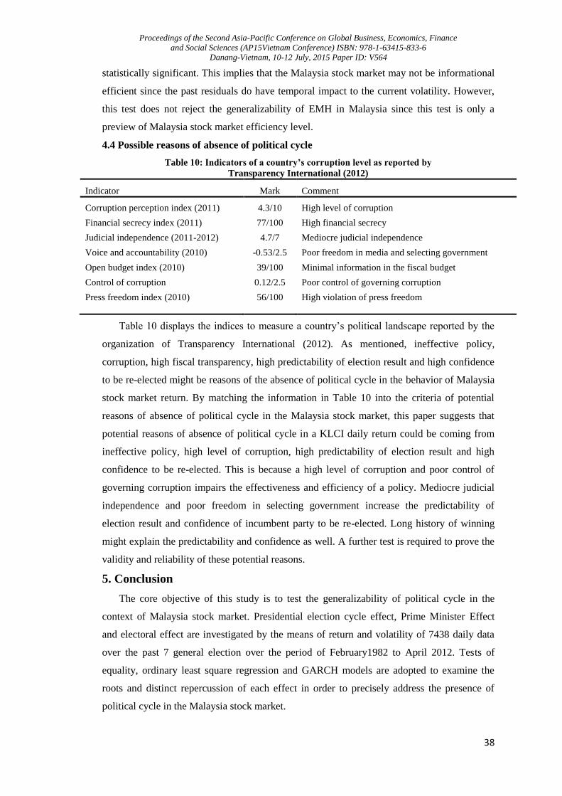
Proceedings of the Second Asia-Pacific Conference on Global Business, Economics, Finance
and Social Sciences (AP15Vietnam Conference) ISBN: 978-1-63415-833-6
Danang-Vietnam, 10-12 July, 2015 Paper ID: V564
38
statistically significant. This implies that the Malaysia stock market may not be informational
efficient since the past residuals do have temporal impact to the current volatility. However,
this test does not reject the generalizability of EMH in Malaysia since this test is only a
preview of Malaysia stock market efficiency level.
4.4 Possible reasons of absence of political cycle
Table 10: Indicators of a country’s corruption level as reported by
Transparency International (2012)
Indicator Mark Comment
Corruption perception index (2011) 4.3/10 High level of corruption
Financial secrecy index (2011) 77/100 High financial secrecy
Judicial independence (2011-2012) 4.7/7 Mediocre judicial independence
Voice and accountability (2010) -0.53/2.5 Poor freedom in media and selecting government
Open budget index (2010) 39/100 Minimal information in the fiscal budget
Control of corruption 0.12/2.5 Poor control of governing corruption
Press freedom index (2010) 56/100 High violation of press freedom
Table 10 displays the indices to measure a country’s political landscape reported by the
organization of Transparency International (2012). As mentioned, ineffective policy,
corruption, high fiscal transparency, high predictability of election result and high confidence
to be re-elected might be reasons of the absence of political cycle in the behavior of Malaysia
stock market return. By matching the information in Table 10 into the criteria of potential
reasons of absence of political cycle in the Malaysia stock market, this paper suggests that
potential reasons of absence of political cycle in a KLCI daily return could be coming from
ineffective policy, high level of corruption, high predictability of election result and high
confidence to be re-elected. This is because a high level of corruption and poor control of
governing corruption impairs the effectiveness and efficiency of a policy. Mediocre judicial
independence and poor freedom in selecting government increase the predictability of
election result and confidence of incumbent party to be re-elected. Long history of winning
might explain the predictability and confidence as well. A further test is required to prove the
validity and reliability of these potential reasons.
5. Conclusion
The core objective of this study is to test the generalizability of political cycle in the
context of Malaysia stock market. Presidential election cycle effect, Prime Minister Effect
and electoral effect are investigated by the means of return and volatility of 7438 daily data
over the past 7 general election over the period of February1982 to April 2012. Tests of
equality, ordinary least square regression and GARCH models are adopted to examine the
roots and distinct repercussion of each effect in order to precisely address the presence of
political cycle in the Malaysia stock market.
Proceedings of the Second Asia-Pacific Conference on Global Business, Economics, Finance
and Social Sciences (AP15Vietnam Conference) ISBN: 978-1-63415-833-6
Danang-Vietnam, 10-12 July, 2015 Paper ID: V564
39
Based on the finding, there is no evidence to prove the pattern of political existing in the
movement pattern of stock market return. Tests of equality and ordinary least square
regression produce homogenous outputs to reject the presence of political cycle in the return
behavior of Kuala Lumpur Composite Index. This finding is similar to study of Ali et. al.
(2010), which was also carried out under the background of Malaysia. This finding suggests
that the government might not be able to convey their objective through the means of policy
implementation. Further, an election does not bring positive surprise to stock market return.
This finding is contrary to major previous studies that examined the relationship between
electoral factors and stock market return.
However, the political cycle and the variance of volatility are found to be significantly
related. This suggests that investors do adjust their portfolio to reflect their views towards the
political factors. For example, the post-election 20-day period is more volatile than the pre-
election 20-days period due to investors adjust their pre-election expectation to actual election
result. This finding is consistent with major previous researches that investigated the
relationship between electoral factors and stock market volatility.
Hence, unique characteristics of a country do oppugn the generalizability of political
cycle in the return behavior of a stock market but not the variance of volatility. The
implication of this study is important to investors who are interested in the Malaysia stock
market. This study serves as guide to investors whether to enter or to exit the Malaysia stock
market. This is because the increase in volatility come from electoral causes does not
compensate by the commensurate increment in the return as the return has been stagnant over
times. For example, investors should avoid the post-election 20-day period due to the
presence of non-value-added volatility.
The gradual decreasing tendency of volatility in the post-election 20-day period calls the
informational efficiency of Malaysia stock market into question. This is because the market
takes considerable time to decode and absorb the election result. Further, this can be proved
by the presence of short-term memory of past residual in the current stock market return.
Hence, the Malaysia stock might not be strongly informational efficient.
6. Limitations and Recommendations for Future Studies
There are several deficiencies that may detrimentally impact the result of this empirical
study. First, this study only compiles the KLCI daily returns of past 7 general elections due to
the data before 1982 is not accessible without incurring considerable costs. Thus, the result of
this paper does not account for the first 5 general elections which could be influential to the
research finding. Further, the use of quarterly and annual data to derive the daily GDP is an
average form of daily change but not the actual change. This issue could impair the
effectiveness of GDP as a conditioning variable to the KLCI daily return.
Proceedings of the Second Asia-Pacific Conference on Global Business, Economics, Finance
and Social Sciences (AP15Vietnam Conference) ISBN: 978-1-63415-833-6
Danang-Vietnam, 10-12 July, 2015 Paper ID: V564
40
Second, different levels of market efficiency between Malaysia and other research
backgrounds may unfavorably influence the research outcome. This is because major research
regarding the political cycle were carried out under the context of developed country with
long history of stock market. Third, a sub-period analysis instead of a whole period analysis
should be applied to take care of the changes in economic and financial background. For
example, 1997 ASEAN financial crisis or pegged- currency exchange rate could change the
return behavior of KLCI. The results obtained from both time-series regression and mean
difference test may be impaired due to the ignorance of these impacts.
For further studies, the sample period should be expanded to include the data before 1982
to examine all past general election. Further, a sub-period method should be adopted to
scrutinize the presence of political cycle in the stock market behavior. More conditioning
variables should be also included to better explain the variance in stock market, such as the
government bill rates.
In a nutshell, although the result is significant, this study may be subject to research errors
due to the unavailability of some required data. The application of the finding of this paper to
the real world should be taken with full care in order to avoid unfavorable outcomes.
References
Abidin, S., Old, C. and Martin, T. (2010) ‘Effects of New Zealand general elections on stock
market returns’, International Review of Business Research Papers, Vol.6, No. 6, pp. 1-12.
Ahmad, Z. H. (1999) ‘Trend in Malaysia: Election assessment’, Institute of Southeast Asian
Studies, No. 1, pp. 1-57.
Alexander, S. S. (1961) ‘Price movement in speculative market - trend or random walk’,
Industrial Management Review, pp. 7-23.
Ali, N.,, Nassir, A. MD., Hassan, T. and Abidin, S. Z. (2010) ‘Short run stock overreaction
evidence from Bursa Malaysia’, International Journal of Economics and Management, Vol. 3,
No. 2, pp. 319-333.
Alt, J. E. and Lessen, D. D. (2006) ‘Transparency, political polarization, and political budget
cycles in OECD countries’, American Journal of Political Science, Vol. 50, No. 3, pp. 530-
550.
Alesina, A. (1987) ‘Macroeconomic policy in a two-party system as a repeated game’.
Quarterly Journal of Economics, Vol. 102, No. 3, pp. 651-678.
Alberto, A. and Sachs, J. (1988) ‘Political parties and the business cycle in the United States,
1948-1984’. Journal of Money, Credit and Banking, Vol. 20, No. 1, pp. 63-82.
Allvine, F. C. and O’Neill, D. E. (1980) ‘Stock market returns and the presidential election
cycle: Implications for market efficiency’, Financial Analysts Journal, Vol. 36, No. 5, pp. 49-
56.
Proceedings of the Second Asia-Pacific Conference on Global Business, Economics, Finance
and Social Sciences (AP15Vietnam Conference) ISBN: 978-1-63415-833-6
Danang-Vietnam, 10-12 July, 2015 Paper ID: V564
41
Altin, H (2012) ‘The effect of electoral periods on the stock market’, International Research
Journal of Finance and Economics, No. 87, pp. 34-47.
Anderson, T. W. and Darling, D. A. (1952) ‘Asymptotic theory of certain "goodness of fit"
criteria based on stochastic processes’, The Annals of Mathematical Statistics, Vol. 23, No. 2,
pp. 193-212.
Anderson, D. R., Sweeney, D. J. and Williams, T. A. (2012) Statistics for Business and
Economics, 11th edition, Cengage Learning.
Ariel, R. A. (1988) ‘A monthly effect in stock returns’, Journal of Financial Economics, Vol.
18, No. 1, pp. 161-174.
Avramov, D. and Chordia, T. (2006) ‘Asset pricing models and financial market anomalies’,
The Review of Financial Studies, Vol. 19, No. 3, pp. 1001-1040.
Baker, M. and Wurgler, J. (2006) ‘Investor sentiment and the cross-section of stock return’,
The Journal of Finance, Vol. 61, No. 4, pp. 1645–1680.
Balkiz, O. (2003) ‘Testing Informational Market Efficiency on Kuala Lumpur Stock
Exchange’, Jurnal Ekonomi Malaysia, No. 37.
Balvers, R. J., Cosimano, T. F. and McDonald, B. (1990) ‘Predicting stock return in an
efficient market’, Journal of Finance, Vol. 45, No. 4, pp. 1109-1128.
Banning, K. and Jones, S. T. (2002) ‘Presidential election cycles and stock market returns’,
The American Academy of Accounting and Finance – conference paper.
Basu, S. (1977) ‘Investment performance of common stocks in relation to their price earnings
ratios - A test of the efficient market hypothesis’, The Journal of Finance, Vol. 32, No. 3, pp.
663-682.
Beaulieu, M. Cosset, J. and Essaddam, N. (2005) ‘The impact of political risk on the volatility
of stock returns: The case of Canada’, Journal of International Business Studies, Vol. 36, No.
6, pp. 701-718.
Beaulieu, M., Cosset, J. and Essaddam, N. (2006) ‘Political uncertainty and stock market
returns: evidence from the 1995 Quebec Referendum’, The Canadian Journal of Economics,
Vol. 39, No. 2, pp. 621-641.
Beechey, M., Gruen, D. and Vickery, J (200) ‘the efficient market hypothesis: A survey’,
Research Discussion Paper.
Beyer, S. B., Jensen, G. R. and Johnson, R. R. (2004) ‘Don't worry about the election - Just
watch the fed’, Journal of Portfolio Management, Vol. 30, No. 4, pp. 101-123.
Bialkowski, J., Gottschalk, K. and Wisniewski, T. P. (2008) ‘Stock market volatility around
national elections’, Journal of Banking & Finance, Vol. 32, No. 9, pp. 1941-1953.
Bittlingmayer, G. (1993) ‘The stock market and the early antitrust law’, Journal of Law and
Economics, Vol. 36, No. 1, pp. 1-32.
Proceedings of the Second Asia-Pacific Conference on Global Business, Economics, Finance
and Social Sciences (AP15Vietnam Conference) ISBN: 978-1-63415-833-6
Danang-Vietnam, 10-12 July, 2015 Paper ID: V564
42
Bittlingmayer, G. (1998) ‘Output, stock volatility, political uncertainty in a natural
experiment: Germany, 1880-1940’, The Journal of Finance, Vol. 53, No. 6, pp. 2243–2257.
Blanchard, O and Perotti, R. (2002) ‘An empirical characterization of the dynamic effects of
changes in government spending and taxes on output’, The Quarterly Journal of Economics,
Vol. 117, No. 4, pp. 1329-1368.
Bohl, M. T. and Gottschalk, K. (2006) ‘International evidence on the Democrat premium and
the presidential cycle effect’, The North American Journal of Economics and Finance, 2006,
vol. 17, no. 2, pp. 107-120.
Bollerslev, T. (1986) ‘Generalized autoregressive conditional heteroskedasticity’, Journal of
Econometrics, Vol. 31, No. 3, pp. 307–327.
Bollerslev, T. and Wooldridge, J. M. (1992) ‘Quasi-maximum likelihood estimation and
inference in dynamic models with time-varying covariances’, Econometric Reviews, Vol. 11,
No. 2, Pages: 143-172.
Bondt, W. F. M. and Thaler, R. (1985) ‘’Does the stock market overreact?’, The Journal of
Finance, Vol. 40, No. 3, pp. 793-805.
Bondt, W. F. M. and Thaler, R. (1987) ‘Further evidence on investor overreaction and stock
market seasonality’, The Journal of Finance, Vol. 42, No. 3, pp. 557-581.
Booth, J. R. and Booth, L. C. (2003) ‘Is presidential cycle in security returns merely a
reflection of business conditions?’ Review of Financial Economics, Vol. 12, No. 2, pp. 131–
159.
Brander, J. A. (1991) ‘Election polls, free trade, and the stock market: Evidence from the
1988 Canadian general election’, The Canadian Journal of Economics, Vol. 24, No. 4, pp.
827-843.
Brandt, M. W. and Kavajecz, K. A. (2004) ‘Price discovery in the US treasury market - The
impact of order flow and liquidity on the yield curve’, The Journal of Finance, Vol. 59, No. 6,
pp. 2623–2654.
Breusch, T. S. (1978) ‘Testing for autocorrelation in dynamic linear model’, Australian
Economic Papers, Vol. 17, No. 31, pp. 334–355.
Brown, S. J. and Warner, J. B. (1982) ‘Using daily stock returns: The case of event studies’,
Journal of Financial Economics, Vol. 14, No. 1, pp. 3–31.
Cahan, J., Malone, C., Powell, J. G. and Choti, U. W. (2005) ‘Stock market political cycles in
a small, two-party democracy’, Applied Economics Letters, Vol. 12, No. 12, pp. 735-740.
Chan, Y. and Wei. K. C. J. (1996) ‘Political risk and stock price volatility: The case of Hong
Kong’, Pacific-Basin Finance Journal, Vol. 4, No. 2–3, pp. 259–275.
Chang, W. and Lai, C (1997) ‘Election outcomes and the stock market: Further results’,
European Journal of Political Economy, Vol. 13, No. 1, pp. 143–155.
Proceedings of the Second Asia-Pacific Conference on Global Business, Economics, Finance
and Social Sciences (AP15Vietnam Conference) ISBN: 978-1-63415-833-6
Danang-Vietnam, 10-12 July, 2015 Paper ID: V564
43
Chia, R. C., Venus, K. Wafa, S. K. and Wafa, S. A. (2006) ‘Calendar anomalies in the
Malaysian stock market’, MPRA Paper, No. 516.
Chopra, N., Lakonishok, J. and Ritter, J. R. (2002) ‘Measuring abnormal performance - Do
stocks overreact’, Journal of Financial Economics, Vol. 31, No. 2, pp. 235–268.
Chowdhury, A. R. (1993) ‘Political surfing over economic waves: Parliamentary election
timing in India’, American Journal of Political Science, Vol. 37, No. 4, pp. 1100-1118.
Chuang, C. and Wang, Y. (2009) ‘Developed stock market reaction to political change: a
panel data analysis’, Quality & Quantity, Vol. 43, No. 6, pp.941-949.
Chuang, C. and Wang, Y. (2010) ‘Electoral information in developed stock market: testing
conditional heteroscedasticity in the market model’, Applied Economics, Vol. 42, No. 9, pp.
1125-1131.
Chukwuogor, C (2008) ‘Stock markets return and volatilities: A global comparison’,
International Research Journal of Finance and Economics, No. 15, pp. 7-30.
Chretien, S. and Coggins, F. (2009) ‘Election outcomes and financial market returns in
Canada’, The North American Journal of Economics and Finance, Vol. 20, No. 1, pp. 1-23.
Collins, D. W. and Hribar, P. (2000) ‘Earnings-based and accrual-based market anomalies:
one effect or two?’ Journal of Accounting and Economics, Vol. 29, No. 1, pp. 101–123.
Cootner, P. H. (1962) ‘Stock price: Random vs. systematic changes’, pp. 24-45.
Cooray, A. (2003) ‘the random walk behavior of stock prices: a comparative study’,
Discussion Paper.
Cowart, A. T. (1978) ‘The economic policies of European governments, part 1 - Monetary
policy’, British Journal of Political Science, Vol. 8, No. 4, pp. 285-311.
Cowart, A. T. (1978) ‘The economic policies of European governments, part 2 - fiscal policy’,
British Journal of Political Science, Vol. 8, No. 4, pp. 425-439.
Crowley, F. D. and Loviscek, A. L. (2002) ‘Assessing the impact of political unrest on
currency returns: A look at Latin America’, The Quarterly Review of Economics and Finance,
Vol. 42, No. 1, pp. 143-153.
Daniel, K. and Titman, S. (2012) ‘Testing factor-model explanations of market anomalies’,
Critical Finance Review, No.1, pp. 103-139.
Dickey, D. A. and Fuller, W. A. (1979) ‘Distribution of the estimators for autoregressive time
series with a unit root’, Journal of the American Statistical Association, Vol. 74, No. 366, pp.
427-431.
Dimson, E. and Mussavian, M, (2000) ‘Market efficiency’, The Current State of Business
Discipline, Vol. 3, pp. 959-970.
Dreman, D. N. and Berry, M. A. (1995) ‘Overreaction, underreact ion and low PE effect’,
Financial Analysts Journal, Vol. 51, No. 4, pp. 21-30.
Proceedings of the Second Asia-Pacific Conference on Global Business, Economics, Finance
and Social Sciences (AP15Vietnam Conference) ISBN: 978-1-63415-833-6
Danang-Vietnam, 10-12 July, 2015 Paper ID: V564
44
Dobson, J. and Dufrene, U. B. (1993) ‘The impacts of U.S. presidential elections on
international security-markets’, Global Finance Journal, Vol. 4, No. 1, pp. 39–47.
Dodd, P. and Warner, J. B. (1983) ‘On corporate governance: A study of proxy contests’,
Journal of Financial Economics, Vol. 11, No. 1–4, pp. 401–438.
Dopke, J and Pierdzioch, C. (2006) ‘Politics and the stock market: Evidence from Germany’,
European Journal of Political Economy, Vol. 22, No. 4, pp. 925-943.
Drazen, A. (2001) ‘The political business cycle after 25 years’, NBER Macroeconomics
Annual 2000, Volume 15, pp. 75-137.
Easaw, J. and Garratt, D. (2000) ‘Elections and UK government expenditure cycles in the
1980s: An empirical analysis’, Applied Economics, Vol. 32, No. 3, pp. 381-391.
Engle, R. F. (1982) ‘Autoregressive conditional heteroscedasticity with estimates of the
variance of United Kingdom inflation’, econometrica, Vol. 50, No. 4, pp. 987-1007.
Engle, R. F. and Ng, V. K. (1993) ‘Measuring and testing the impact of news on volatility’,
The Journal of Finance, Vol. 48, No. 5, pp. 1749-1778.
Evans, J. L. (1968) ‘The random walk hypothesis, portfolio analysis and buy-and-hold
strategy’, Journal of Financial and Quantitative Analysis, Vol. 3, No. 3, pp. 327-342.
Fama, E. F. (1965) ‘The behavior of stock-market prices’, The Journal of Business, Vol. 38,
No. 1, pp. 34-105.
Fama, E. F. (1970) ‘Efficient capital market: A review of theory and empirical work’, Journal
of Finance, Vol. 25, No. 2, pp. 383-417.
Fama, E. F. and French, K. R. (1988) ‘Permanent and temporary components of stock prices’,
The Journal of Political Economy, Vol. 96, No. 2., pp. 246-273.
Fama, E. F. (1991) ‘efficient capital market: 2’, Journal of Finance, Vol. 46, No. 5, pp. 1575-
1617.
Fama, E. F. (1995) ‘Random walk in stock market prices’, Financial Analysts Journal, Vol.
51, No. 1, pp.75-80.
Fama, E. F. (1998) ‘Market efficiency, long-term returns, and behavioral finance’, Journal of
Financial Economics, Vol. 49, No. 3, pp. 283–306.
Fay, M. P. and Proschan, M. A. (2010) ‘Wilcoxon-Mann-Whitney or t-test? On assumptions
for hypothesis tests and multiple interpretations of decision rules’, Statistics Surveys, Vol. 4,
pp. 1–39.
Ferri, M. Q. (2008) ‘The response of US equity values to the 2004 presidential election’,
Journal of Applied Finance, Vol. 18, No. 1, pp. 29-37.
Ferson, W. E., Heuson, A. and Su, T. (2005) ‘Weak-form and semi strong-form efficiency
market return predictability’, Management Science, Vol. 51, No. 10, pp. 1582-1592.
Floros, C. (2008) ‘The influence of the political elections on the course of the Athens Stock
Exchange 1996-2002’, Managerial Finance, Vol. 34, No. 7, pp. 479-488.
Proceedings of the Second Asia-Pacific Conference on Global Business, Economics, Finance
and Social Sciences (AP15Vietnam Conference) ISBN: 978-1-63415-833-6
Danang-Vietnam, 10-12 July, 2015 Paper ID: V564
45
Foerster, S. R. and Schmitz, J. J. (1997) ‘The transmission of U.S. election cycles to
international stock returns’, Journal of International Business Studies, Vol. 28, No. 1, pp. 1-
27.
French, K. R. (1980) ‘Stock returns and the weekend effect’, Journal of Financial Economics,
Vol. 8, No. 1, pp. 55–69.
Fuss, R. and Bechtel, M. M. (2008) ‘Partisan politics and stock market performance: The
effect of expected government partisanship on stock returns in the 2002 German federal
election’, Public Choice, Vol. 135, No. 3-4, pp. 131-150.
Gartner, M. and Wellershoff, K. W. (1995) ‘Is there an election cycle in American stock
returns?’, International Review of Economics & Finance, Vol. 4, No. 4, pp. 387–410.
Gilson, R. J. and Kraakman, R. H. (1984) ‘The mechanisms of market efficiency’, Virginia
Law Review, Vol. 70, No. 4, pp. 549-644.
Godfrey, L. G. (1978) ‘Testing against general autoregressive and moving average error
models when the regressors include lagged dependent variables’, Econometrica, Vol. 46, No.
6, pp. 1293-1301.
Goldman, E (2000) ‘Testing efficient market hypothesis for the dollar–sterling gold standard
exchange rate 1890–1906: MLE with double truncation’, Economics Letters, Vol. 69, No. 3,
pp. 253–259.
Grant, J. L. and Trahan, E. A. (2006) ‘Tactical asset allocation and presidential elections’,
Financial Services Review, No. 15, pp. 151–165.
Green, T. C. (2004) ‘Economic news and the impact of trading on bond prices’, The Journal
of Finance, Vol. 59, No. 3, pp. 1201-1233.
Grier, K. B. (1989) ‘On the existence of a political monetary cycle’, American Journal of
Political Science, Vol. 33, No. 2, pp. 376-389.
Hamid, K., Suleman, M. T., Shah, S. Z. A. and Akash, R. S. I. (2010), ‘testing the weak-form
of efficient market hypothesis: Empirical evidence from Asia-Pacific markets’, International
Research Journal of Finance and Economics, No. 58. pp. 121-133.
Hawawini, G. and Keim, D. B. (1995) ‘On the predictability of common stock return - world-
wide evidence’, Handbooks in Operations Research and Management Science, Vol. 9, 1995,
pp. 497–544.
Haug, M and Hirschey, M (2006) ‘The January effect’, Financial Analysts Journal, Vol. 62,
No. 5, pp. 78-88.
He, Y., Lin, H., Wu, C. and Dufrene, U. B. (2009) ‘The 2000 presidential election and the
information cost of sensitive versus non-sensitive S&P 500 stocks’, Journal of Financial
Markets, Vol. 12, No. 1, Pages 54-86.

Proceedings of the Second Asia-Pacific Conference on Global Business, Economics, Finance
and Social Sciences (AP15Vietnam Conference) ISBN: 978-1-63415-833-6
Danang-Vietnam, 10-12 July, 2015 Paper ID: V564
46
Hensel, C. R. and Ziemba, W. T. (1995) ‘United States investment returns during Democratic
and Republican administrations, 1928-1993’, Financial Analysts Journal, Vol. 51, No. 2, pp.
61-69.
Herbst, A. F. and Slinkman, C. W. (1984) ‘Political-economic cycle in the U.S. stock market’,
Financial Analysts Journal, Vol. 40, No. 2, pp. 38-44.
Herron, M. C., Lavin, J., Cram, D. and Silver, J. (1999) ‘Measurement of political effects in
the United States economy: A study of the 1992 presidential election’, Economics and
Politics, Vol. 11, No. 1, pp. 51–81.
Hibbs, Jr. D. A (1977), ‘Political parties and macroeconomic policy’, The American Political
Science Review, Vol. 71, No. 4, pp. 1467-1487.
Hibbs, Jr. D. A (1986) ‘Political parties and macroeconomic policies and outcomes in United
States’, The American Economic Review, Vol. 76, No. 2, pp. 66-70.
Hobbs, G. R. and Riley, W. B. (1984) ‘Profiting from a presidential election’, Financial
Analysts Journal, Vol. 40, No. 2, pp. 46-52.
Huang, R. D. (1985) ‘Common stock returns and presidential elections’, Financial Analysts
Journal, Vol. 41, No. 2, pp. 58-61.
Hudson, R. and Keasey, K. and Dempsey, M (1998): Share prices under Tory and Labour
governments in the UK since 1945, Applied Financial Economics, Vol. 8, No. 4, pp. 389-400.
Hunter, J. E. and Coggin, T. A. (1988) ‘Analyst judgment - The efficient market hypothesis
versus a psychological theory of human judgment’, Organizational Behavior and Human
Decision Processes, Vol. 42, No. 3, pp. 284-302.
Iachine, I., Peterson, H. C. and Kyvik, K. O. (2004) ‘Robust tests for the equality of variances
for clustered data’, University of Southern Denmark – published paper.
Jacobsen, B. (1999) ‘Irrational trading in financial market’, is working paper.
Jarque, C. M. and Bera, A. K. (1980) ‘Efficient tests for normality, homoscedasticity and
serial independence of regression residuals’, Economics Letters, Vol. 6, No. 3, pp. 255–259.
Jarque, C. M. and Bera, A. K. (1987) ‘A test for normality of observations and regression
residuals’, International Statistical Review, Vol. 55, No. 2, pp. 163-172.
Jensen, G. R., Mercer, J. M. and Johnson, R. R. (1996) ‘Business conditions, monetary policy,
and expected security returns’, Journal of Financial Economics, Vol. 40, No. 2, pp. 213-237.
Jensen, M. C. (1978) ‘Some anomalous evidence regarding market efficiency’, Journal of
Financial Economics, Vol. 6, No. 2–3, pp. 95–101.
Jensen, M. C. and Benington, G. A. (1970) ‘Random walks and technical theories: Some
additional evidence’, Journal of Finance, Vol. 25, No. 2, pp. 469-482.
Jones, S. T. and Banning, K. (2009) ‘US elections and monthly stock market returns’, Journal
of Economics and Finance, Vol. 33, No. 3, pp. 273-287.
Proceedings of the Second Asia-Pacific Conference on Global Business, Economics, Finance
and Social Sciences (AP15Vietnam Conference) ISBN: 978-1-63415-833-6
Danang-Vietnam, 10-12 July, 2015 Paper ID: V564
47
Johnson, P., Lynch, F. and Walker, J. G. (2005) ‘Income tax and elections in Britain, 1950–
2001’, Electoral Studies, Vol. 24, No. 3, pp. 393-408.
Johnson, R. and Chittenden, W. T. and Jensen, G. R. (1999) ‘Presidential politics, stocks,
bonds, bills, and inflation’, The Journal of Portfolio Management, Vol. 26, No. 1, pp. 27-31.
Johnson, R. and Soenen, L. (2003) ‘Economic integration and stock market co-movement in
the Americas’, Journal of Multinational Financial Management, Vol. 13, No. 1, pp. 85-100.
Kan, D. and Callaghan, B. A. (2007) ‘Examination of the efficient market hypothesis—the
case of post-crisis Asia Pacific countries’, Journal of Asian Economics, Vol 18, No. 2, pp.
294–313.
Kayser, M. A. (2005) ‘Who surfs, who manipulates - the determinant of opportunistic election
timing and electorally motivated economic intervention’, American Political Science Review,
Vol. 99, No. 1, pp. 17-27.
Kearney, C. (2000) ‘The determination and international transmission of stock market
volatility’, Global Finance Journal, Vol. 11, No. 1–2, pp. 31-52.
Keim, D. B. (1983) ‘Size-related anomalies and stock return seasonality: Further empirical
evidence’, Journal of Financial Economics, Vol. 12, No. 1, pp. 13–32.
Keim, D. B. and Stambaugh, R. F. (1986) ‘Predicting returns in the stock and bond markets’,
Journal of Financial Economics, Vol. 17, No. 2, pp. 357-390.
Kim, H. Y. and Mei, J. P. (2001) ‘What makes the stock market jump? An analysis of
political risk on Hong Kong stock returns’, Journal of International Money and Finance, Vol.
20, No. 7, pp. 1003–1016.
Kithinji, A. and Ngugi, W. (2008) ‘Stock market performance before and after elections – a
case study of the Nairobi Stock Exchange’, MBA project.
Knight, B (2004) ‘Are policy platforms capitalized into equity prices? Evidence from the
bush/gore 2000 presidential election’, National Bureau of Economic Research – working
paper.
Koulakiotis, A., Dasilas, A. and Tolikas, K. (2008) ‘Political elections and stock price
volatility: The case of Greece’, The European Financial Management Association - published
paper.
Kraussl, R., Lucas, A., Rijsbergen, D. R., Sluis, P. J. and Vrugt, E. B. (2008) ‘Washington
meets Wall Street: A closer examination of the presidential cycle puzzle’, Tinbergen Institute
- Discussion Paper No. 08-101/2.
Lakonishok, J. and Smidt, S. (1988) ‘Are seasonal anomalies real - A ninety-year perspective’,
The Review of Financial Studies, Vol. 1, No. 4, pp. 403-425.
Leblang, D. and Mukherjee, B. (2004) ‘Presidential elections and the stock market -
comparing markov-switching and garch models of stock volatility’, Political Analysis, Vol.
12, No. 3, pp. 296-322.
Proceedings of the Second Asia-Pacific Conference on Global Business, Economics, Finance
and Social Sciences (AP15Vietnam Conference) ISBN: 978-1-63415-833-6
Danang-Vietnam, 10-12 July, 2015 Paper ID: V564
48
Leblang, D. and Mukherjee, B. (2005) ‘Government partisanship, elections and the stock
market - examining American and British stock return, 1930-2000’, Journal of Political
Science, Vol. 49, No. 4, pp. 780-802.
Lee, C. and Lee, J. (2009) ‘Energy prices, multiple structural breaks and efficient market
hypothesis’, Applied Energy, Vol. 86, No. 4, pp. 466–479.
Lee, C., Lee, J. and Lee, C. (2009) ‘Stock prices and the efficient market hypothesis:
Evidence from a panel stationary test with structural breaks’, Japan and the World Economy,
Vol. 22, No. 1, pp. 49-58.
Levene, H. (1960) ‘Robust tests for equality of variances’, In I. Olkin(Ed.), Contributions to
Probability and Statistics, pp. 278–292. Palo Alto, California: Stanford University Press; as
cited in Iachine, I., Peterson, H. C. and Kyvik, K. O. (2004) ‘Robust tests for the equality of
variances for clustered data’, University of Southern Denmark – published paper.
Li, J. and Born, J. A. (2006) ‘Presidential election uncertainty and common stock returns in
the United States’, Journal of Financial Research, Vol. 29, No. 4, pp. 609–622.
Lim, K. S. (1991) ‘The dirtiest general elections in the history of Malaysia’, Speech by the
Democratic Action Party, published by Oriengroup Sdn. Bhd.
Lim, S. Y., Ho, C. H. and Dollery, B. (2007) ‘Stock market calendar anomalies: The case of
Malaysia’, Working Paper.
Lin, C and Wang, Y (2005) ‘An analysis of political changes on Nikkei 225 stock returns and
volatilities’, Annals of Economics and Finance, Vol. 6, pp.169-183.
Liu, B and Li, B. (2010) ‘Day to the week effect - Another evidence from top 50 Australian
stocks’, European Journal of Economics, Finance and Administrative Sciences, Vol. 2010, No.
24, pp. 78-87.
Ljung, G. M. and Box, G. E. P. (1978) ‘On a measure of lack of fit in time series models’,
Biometrika, Vol. 65, No. 2, pp. 297-303.
Lo, A. W. and McKinlay, A. C. (1988) ‘ Stock market prices do not follow random walks:
evidence from a simple specification test’, The Reviews of Financial Studies, Vol. 1, No. 1, pp.
41-66.
Lutkepohl, H. (1991), “Introduction to Multiple Time Series Analysis”, Springer-Verlag; as
cited in Chia, R. C., Venus, K. Wafa, S. K. and Wafa, S. A. (2006) ‘Calendar anomalies in the
Malaysian stock market’, MPRA Paper, No. 516.
MacRae, C. D. (1977) ‘A political model of the business cycle’, Journal of Political Economy,
Vol. 85, No. 2, pp. 239-263.
Malkiel, B. G. (2003) ‘The efficient market hypothesis and its critics’, Journal of Economic
Perspectives, Vol.17, No. 1, pp. 59 – 82.
Proceedings of the Second Asia-Pacific Conference on Global Business, Economics, Finance
and Social Sciences (AP15Vietnam Conference) ISBN: 978-1-63415-833-6
Danang-Vietnam, 10-12 July, 2015 Paper ID: V564
49
Malkiel, B. G. (2005) ‘Reflections on the efficient market hypothesis: 30 years later’,
Financial Review, Vol. 40, No. 1, pp. 1–9.
Mann, H. B. and Whitney, D. R. (1947) ‘On a test of whether one of two random variables is
stochastically larger than the other’, The Annals of Mathematical Statistics, Vol. 18, No. 1, pp.
50-60.
Marquardt, D. W. (1970) ‘Generalized inverses, ridge regression, based linear estimation, and
nonlinear estimation’, Techno metrics, Vol. 12, No. 3, pp. 591-612.
McCallum, B. T. (1978) ‘the political business cycle: An empirical test’, Southern Economic
Journal, Vol. 44, No. 3, pp. 504-515.
McGillibray, F. (2001) ‘Government hand-outs, political institutions and stock price
dispersion’, Yale University – working paper.
Mevorach, B. (1989) ‘The political monetary business cycle political reality and economic
theory’, Political Behavior, Vol. 11, No. 2, pp. 175-188.
Mlambo, C. and Biekpe, N. (2007) ‘The efficient market hypothesis: Evidence from ten
African stock markets’, Investment Analysts Journal, No. 66, pp. 5-18.
Mobarek, A., Mollah, A. S. and Bhuyan, R. (2008) ‘Market efficiency in emerging stock
market: Evidence from Bangladesh’, Journal of Emerging Market Finance January, Vol. 7,
No. 1, pp. 17-41.
Nadeau, R. and Lewis-Beck, M. S. (2001) ‘National economic voting in U.S. presidential
elections’, The Journal of Politics, Vol. 63, No. 1, pp. 159-181.
Nelson, D. B. (1991) ‘Conditional heteroskedasticity in asset returns: A new approach’,
Econmetrica, Vol.39, No. 2, pp. 347-370.
Newey, W. K. and West, K. D. (1987) ‘A simple, positive semi-definite, heteroskedasticity
and autocorrelation consistent covariance matrix’, Econometrica, Vol. 55, No. 3, pp. 703-708.
Nguyen, A. and Roberge, M (2008),"Timing the stock market with a joint examination of the
presidential election cycle and the yield curve", Studies in Economics and Finance, Vol. 25,
No. 3 pp. 152 – 164.
Niederhoffer, V., Gibbs, S. and Bullock, J. (1970) ‘Presidential election and the stock market’,
Financial Analysts Journal, Vol. 26, No. 2, pp. 111-113.
Nippani, S. and Arize, A. C. (2005) ‘US presidential election impact on Mexican and
Canadian stock market’, Journal of Economics and Finance, Vol. 29, No. 2, pp. 271-279.
Nordhaus, W. D. (1975) ‘The political business cycle’, The Review of Economic Studies, Vol.
42, No. 2, pp. 169-190.
Nordhaus, W. D., Alesina, A. and Schultze, C. L. (1989) ‘Alternative approach to the political
business cycle’, Brookings Papers on Economic Activity, Vol. 1989, No. 2, pp. 1-68.
Okpara, G. C. (2010) ‘Stock market prices and the random walk hypothesis: Further evidence
from Nigeria’, Journal of Economics and International Finance, Vol. 2, No. 3, pp. 49-57.
Proceedings of the Second Asia-Pacific Conference on Global Business, Economics, Finance
and Social Sciences (AP15Vietnam Conference) ISBN: 978-1-63415-833-6
Danang-Vietnam, 10-12 July, 2015 Paper ID: V564
50
Pantzalis, C. Stangeland, D. A. and Turtle, H. J. (2000) ‘Political elections and the resolution
of uncertainty: The international evidence’, Journal of Banking & Finance, Vol. 24, No. 10,
pp. 1575-1604.
Parra, S. N. and Santiso, J. (2008) ‘Wall street and elections in Latin American emerging
democracies’, OECD working paper, No. 272.
Phillips, P. C. B. and Perron, P. (1988) ‘Testing for a unit root in time series regression’,
Biometrika, Vol. 75, No. 2, pp. 335-346.
Ploeg, F. (1984) ‘Government ideology and re-election efforts’, Oxford Economic Papers,
Vol. 36, No. 2, pp. 213-231.
Ploeg, F. (1989) ‘Election outcomes and the stockmarket’, European Journal of Political
Economy, Vol. 5, No. 1,pp. 21–30.
Powell, J. G., Shi, J., Smith, T. and Whaley, R. E. (2007) ‘The persistent presidential dummy’,
The Journal of Portfolio Management, Vol. 33, No. 2, pp. 133.
Rajaratnam, U. D. (2009) ‘Role of traditional and online media in the 12th general election,
Malaysia’, The Journal of the South East Asia Research, Vol. 1, No. 1, pp. 33-58.
Riley, W. B. and Luksetich, W. A. (1980) ‘the market prefers republicans: Myth or reality’,
The Journal of Financial and Quantitative Analysis, Vol. 15, No. 3, pp.541-560.
Ritter, J. R. (2003) ‘Behavioral finance’, Pacific-Basin Finance Journal, Vol. 11, No. 4, pp.
429-437.
Rosenberg, M. (2004) ‘The monthly effect in stock returns and conditional heteroscedasticity’,
The American Economist, Vol. 48, No. 2, pp. 67-73.
Santa-Clara, P. and Valkanov, R. (2003) ‘The presidential puzzle: Political cycle and the
stock market’, The Journal of Finance, Vol. 58, No. 5, pp. 1841-1872.
Schlater, J. E., Haugen, R. A. and Wichern, W. W. (1980) ‘Trading based on forecasts of
earnings per share: A test of the efficient market hypothesis’, Journal of Banking & Finance,
Vol. 4, No. 2, pp. 197–211.
Schultz, K. A. (1995) ‘The politics of the political business cycle’, British Journal of Political
Science, Vol. 25, No. 1, pp. 79-99.
Schwars, G. (1978) ‘Estimating the dimension of a model’, The Annals of Statistics, Vol. 6,
No. 2, pp. 461-464.
Schwert, G. W. (2003) ‘Anomalies and market efficiency’, Handbook of the Economics of
Finance, Vol. 1, Part B, pp. 939–974.
Proceedings of the Second Asia-Pacific Conference on Global Business, Economics, Finance
and Social Sciences (AP15Vietnam Conference) ISBN: 978-1-63415-833-6
Danang-Vietnam, 10-12 July, 2015 Paper ID: V564
51
Sellin, P. (2002) ‘Monetary policy and the stock market: Theory and empirical evidence’,
Journal of Economic Surveys, Vol. 15, No. 4, pp. 491–541.
Siokis, F. and Kapopoulos, P. (2007) ‘Parties, elections and stock market volatility - evidence
from a small open economy’, Economics & Politics, Vol. 19, No. 1, pp. 123–134.
Stovall, R. H. (1992) ‘Forecasting stock market price’, Financial Analysts Journal, Vol. 48,
No. 3, pp. 5-8.
Sturm, R. R. (2011) ‘Economic policy and the presidential election cycle in stock returns’,
Journal of Economics and Finance.
Swensen, R. B. and Patel, J. B. (2004) ‘NYSE sector returns and political cycles’, Journal of
Business Ethics, Vol. 49, No. 4, pp. 387-395.
Thorbecke, W (1997) ‘On stock market returns and monetary policy’, The Journal of Finance,
Vol. 52, No. 2, pp. 635-654.
Timmerman, A. and Granger, C. W. J. (2004) ‘Efficient market hypothesis and forecasting’,
International Journal of Forecasting, Vol. 20, No. 1, pp. 15–27.
Transparency International (2012), Organization, Available at URL:
http://www.transparency.org/country#MYS_DataResearch
Umstead, D. A. (1977) ‘Forecasting stock market price’, The Journal of Finance, Vol. 32, No.
2, pp. 427-441.
Uri, N. D. and Jones, J. D. (1990) ‘Are the markets for financial assets efficient?: Evidence
for the USA, 1974–1988’, Economic Modeling, Vol. 7, No. 4, pp. 388–394.
Vaaler,P. M., Schrage, B. N. and Block, S. A. (2005) ‘Counting the investor vote: Political
business cycle effects on sovereign bond spreads in developing countries’, Journal of
International Business Studies, Vol. 36, No. 1, pp. 62-88.
Welch, I. (2000) ‘Views of financial economists on the equity premium and on professional
controversies’, The Journal of Business, Vol. 73, No. 4, pp. 501-537.
White, H. (1980) ‘A heteroskedasticity-consistent covariance matrix estimator and a direct
test for heteroskedasticity’, Econometrica, Vol. 48, No. 4, pp. 817-838.
Wong, W. and McAleer, M. (2009) ‘Mapping the presidential election cycle in US stock
markets’, Mathematics and Computers in Simulation, Vol. 79, No. 11,pp. 3267-3277.
Wong, Y., Lee, M. and Lin, C. (2008) ‘General election, political change and market
efficiency: Long- and short-term perspective in developed stock market’, Journal of Money,
Investment and Banking, No. 3, pp. 58-67.
Worthington, A. C. (2006) ‘Political cycles in the Australian stock market since Federation’,
Faculty of Commerce – Papers.
Worthington, A. C. (2006) ‘Political cycles and risk and return in the Australian stock market,
Menzies to Howard’, University of Wollongong – working paper.

Proceedings of the Second Asia-Pacific Conference on Global Business, Economics, Finance
and Social Sciences (AP15Vietnam Conference) ISBN: 978-1-63415-833-6
Danang-Vietnam, 10-12 July, 2015 Paper ID: V564
52
Worthington, A. C. and Higgs, H. (2006) ‘Weak-form market efficiency in Asian emerging
and developed equity markets: Comparative tests of random walk behavior’, Faculty of
Commerce – Papers.
Yalcn, K. C. (2010) ‘Market rationality: Efficient market hypothesis versus market
anomalies’, European Journal of Economic and Political Studies, Vol. 3, No. 2, pp. 23-38.
Yantek, T. and Cowart, A. T. (1986) ‘Elections and Wall Street: Taking Stock of Parties and
Presidents’, The Western Political Quarterly, Vol. 39, No. 3, pp. 390-412.
Zhao, X., Liano, K. and Hardin III, W. G. (2004) ‘Presidential election cycles and the turn-of-
the-month effect’, Social Science Quarterly, Vol. 85, No. 4, pp. 958-973.