POLITICAL BUSINESS CYCLES IN THE NEW KEYNESIAN MODEL

POLITICAL BUSINESS CYCLES IN THE NEW KEYNESIAN MODEL

FABIO MILANI*

This paper tests various political business cycle theories in a New Keynesian modelwith a monetary and fiscal policy mix. All the policy coefficients, the target levels ofinflation and the budget deficit, the firms’ frequency of price setting, and the standarddeviations of the structural shocks are allowed to depend on ‘‘political’’ regimes:a preelection versus postelection regime, a regime that depends on whether thepresident (or the Fed chairman) is a Democrat or a Republican, and a regimeunder which the president and the Fed chairman share party affiliation inpreelection quarters or not. The results provide evidence that several coefficients areinfluenced by political variables. The best-fitting specification, in fact, is one thatallows coefficients to vary according to a regime that depends on whether theeconomy is in the few quarters before a presidential election or not. Monetarypolicy becomes considerably more inertial before elections and fiscal policydeviations from a simple rule are more common. There is some evidence thatpolicies become more expansionary before elections, but this evidence disappears formonetary policy in the post-1985 sample. (JEL C11, D72, E32, E52, E58, E63)

‘‘Iknowthere’sthemythoftheautonomousFed . . .’’Nixon barked a quick laugh.

—Richard Nixon, talking to Arthur Burnson October 23, 1969, just after Burns’s nomi-nation to the Fed had been announced.1

‘‘I’d like to see another lowering of interest rates.I think there’s room to do that. I can understandpeople worrying about inflation. But I don’t thinkthat’s the big problem now.’’

—George H. W. Bush, interview withNew York Times, June 24, 1992.

I. INTRODUCTION

Economic conditions before elections affectelection outcomes.2 Rational politicians who

recognize this regularity may, therefore, betempted to try to influence the economy inthe quarters preceding an election date tomaximize their chances of being reelected.

The literature on political business cycles(PBC) has developed models that rationalizeeconomic fluctuations induced by politicalcycles. Nordhaus (1975) presented a modelof ‘‘opportunistic’’ political cycles: the partyin power stimulates the economy before elec-tions to improve its reelection probability.Others have observed that different partiesmay have different preferences over inflationand output or unemployment outcomes and,therefore, we should observe ‘‘partisan’’political cycles. Hibbs (1977) was the first tointroduce the partisan cycle model, in whichleft-wing parties were assumed to have at leastone of the following: a higher output target,a higher inflation target, or a higher relativeweight on minimizing output rather than

*I would like to thank the editor and two anonymousreferees, as well as Michelle Garfinkel, Ami Glazer, KevinGrier, and my conference discussants Fabio Mendez andRodrigo Martins for helpful comments and suggestions.

Milani: Assistant Professor, Department of Economics,University of California, 3151 Social Science Plaza,Irvine, CA 92697-5100. Phone 949-824-4519, Fax 949-824-2182, E-mail [email protected], Homepage: http://www.socsci.uci.edu/;fmilani

1. Abrams (2006).2. Kramer (1971), Tufte (1975, 1978), Fair (1978),

Blomberg and Hess (2003), and Alesina, Londregan,and Rosenthal (1993) provide evidence that favorable eco-nomic conditions in the quarters prior to a presidentialelection enhance the probability of the incumbent’s beingreelected.

ABBREVIATIONS

DSGE: Dynamic Stochastic General

Equilibrium

FOMC: Federal Open Market Committee

GDP: Gross Domestic Product

PBC: Political Business Cycles

PLM: Perceived Law of Motion

Economic Inquiry doi:10.1111/j.1465-7295.2009.00212.x

(ISSN 1465-7295) � 2009 Western Economic Association International

1

inflation deviations from the targets, com-pared with right-wing parties.

Several papers test for the existence ofopportunistic or partisan cycles in the UnitedStates. Alesina, Cohen, and Roubini (1992)and Alesina, Roubini, and Cohen (1997) findonly weak evidence of an opportunistic polit-ical cycle looking at M1 growth rates. Grier(1989) and Beck (1987), instead, find supportfor the effect of political variables on M1growth rates for the 1960–1980 period, butnot on the mean level of the federal funds rate.As discussed in Drazen (2000a, 2000b), there isbasically no evidence, instead, that politicalcycles matter for macroeconomic outcomesby looking at data on unemployment and out-put growth (Grier 2008 is a recent exception),and only weak evidence for inflation.

Empirical tests of the partisan cycle model(Alesina, Roubini, and Cohen 1997; Faust andIrons 1999) find partisan differences in outputgrowth rates, but no support for partisancycles in inflation and monetary policy.

Tests of PBC typically assume monetarypolicy as the main tool that is exploited by pol-iticians to manipulate the economy. Thesestudies usually focus on comparing the levelof inflation, output, money growth rates, orinterest rates across political cycles, or theyadd a political dummy variable to the relevantregression and test its significance.

This paper offers a different approach. Thepaper aims to empirically test various politicalbusiness cycle theories adopting an optimizingNew Keynesian model with a monetary andfiscal policy mix as the main setting (the inclu-sion of both fiscal and monetary policy ismotivated by Drazen 2000b).3 The NewKeynesian model is a baseline setting for theanalysis of monetary policy, but it has notbeen widely used to study PBC. An advantageof this paper with respect to most of the pre-vious PBC literature lies in the use of a generalequilibrium framework: this is, in fact, neces-

sary when testing the importance of politicallymotivated policy choices to effectively controlfor differences in the macroeconomic condi-tions, the set of shocks, or the private sectorexpectations that prevail when the policydecision is taken.

The monetary and fiscal policy rule param-eters, as well as the parameters that reflect thefrequency of price adjustment by firms and thesteady-state level of inflation, are allowed todepend on the (observed) political regime.

Several hypotheses can, therefore, betested. The coefficients may, in fact, differ inpreelection versus no-election periods, theymay depend on the party affiliation of eitherthe president or the Federal Reserve chair-man, and on whether the president and theFed chairman share the same affiliation ornot in a preelection period (the different casesare introduced one at a time in the model tosave degrees of freedom).

Political cycles in monetary and fiscal pol-icy are tested by looking at the various policyfeedback coefficients rather than at the meanlevels of outcome variables or money growthrates as often done in the literature. The paperis, therefore, more closely related to recentstudies by Krause and Mendez (2005), whotry to infer policy makers’ revealed preferencestoward inflation and output stability and testwhether these are affected by the proximity toelections or by the ruling party’s ideology, andby Abrams and Iossifov (2006), who use aTaylor rule during the 1957–2004 sample totest political cycle theories. Abrams and Iossi-fov use a single equation approach, while thispaper employs a full-information Bayesianapproach to estimate a general equilibriummodel with both monetary and fiscal policy.The paper is also related to Faust and Irons(1999), who estimate an identified vectorautoregression (VAR) in which the coeffi-cients are contingent on the regime. The cur-rent paper, instead, uses a structural model tojudge the importance of political regimes. Thestructural model is considerably more parsi-monious than Faust and Irons’ VAR andallows for an easier interpretation of thecoefficients.

If political cycles were important, agentsshould be able to incorporate this informationinto their expectations. Under the conven-tional assumption of rational expectations,however, agents would be assumed to knowthat political cycles exist and to have known

3. Drazen (2000b) reviews the evidence accumulatedin 25 yr of political business cycle research and concludesthat models based on monetary policy are not entirely con-vincing; he argues that a larger focus on fiscal policy, oftendisregarded in the literature, may prove more promising.There is evidence, in fact, that fiscal transfers are manip-ulated to gain an electoral advantage (Tufte, 1978; Keechand Pak, 1989; Alesina, 1988). Moreover, the use of mon-etary policy as the main driving force may be problematicsince politicians typically do not have full control of mon-etary policy, this task being left to independent centralbanks.

2 ECONOMIC INQUIRY

this for the whole sample period. Besides, theywould also have perfect knowledge about the‘‘size’’ of the political cycle effect and, underpartisan cycles, about the different politicalparties’ objective functions.

These are, of course, strong informationalassumptions. In this paper, I relax rationalexpectations, by assuming that economic sub-jects have to learn about economic relation-ships over time (in the spirit of the adaptivelearning literature; e.g., Evans and Honka-pohja 2001). In this specification, the agentsare allowed to learn from past observationshow PBC affect fluctuations in output, infla-tion, and future policies. From a more em-pirical point of view, learning introducestime variation in the model, which helpsfitting macroeconomic data, again in a veryparsimonious way.

The model is estimated using likelihood-based Bayesian methods on postwar U.S.data. The estimation approach follows Milani(2007), who shows how to estimate a dynamicstochastic general equilibrium (DSGE) modelwith near-rational expectations and learning.The Bayesian approach facilitates the jointestimation of the learning parameters togetherwith the ‘‘deep’’ parameters of the economyand the policy feedback parameters. In thisway, the learning process is jointly extrapo-lated from the data, rather than imposed a pri-ori and the analysis conditioned on it. Therelevance of different PBC theories can thenbe gauged by looking at how the parameters’posterior distributions vary across regimesand by comparing the marginal likelihoodsof the alternative model specifications.

A. Results

The results are supportive of the notionthat political variables matter. Several policyparameters, as well as some of the economy’sstructural parameters, vary across politicalregimes. The best-fitting specification is onein which the relevant political regime is definedby whether the economy is in the few quarterspreceding a presidential election or not.

The results show that monetary policybecomes extremely inertial before the election.The rarity of policy changes is consistent withan independent Fed, which is also concernedabout giving an impression of not actively par-ticipating in the political race. Apart from the

inertia, there is some evidence, although notstrong, that both monetary policy (but onlybefore 1979) and fiscal policy become moreexpansionary before elections.

This paper aims to add to the empirical lit-erature on PBC. But the paper can also be seenas a contribution to empirical studies of theNew Keynesian model aimed at testing whetherthe exclusion of political variables may haverepresented an important misspecification ofthe model. The paper is finally related to theliterature that studies the monetary–fiscalpolicy mix (e.g., Favero and Monacelli 2005;Muscatelli, Tirelli, and Trecroci 2004) andto empirical applications of models with adap-tive learning (e.g., Adam 2005; Milani 2007;Orphanides and Williams 2005).

II. THE MODEL

I assume that the aggregate dynamics of theeconomy can be summarized by the followingNew Keynesian model, which is widely used tostudy monetary policy issues and which can bederived from the optimizing decisions of eco-nomic agents (see Woodford 2003, for a stan-dard derivation):

xt 5 Etxtþ1 � rðit � Etptþ1 � rtN Þð1Þ

pt � p*ðStÞ 5 bEtðptþ1 � p*ðStÞÞ

þ jðStÞxt þ ut

ð2Þ

it 5 qMPðStÞit�1 þ ð1� qMPðStÞÞ½rNtþ p*ðStÞ þ vpðStÞðpt�1 � p*ðStÞÞ

þ vxðStÞxt�1� þ et

ð3Þ

dt 5 qFPðStÞdt�1 þ ð1� qFPÞðStÞ½s0ðStÞþ sBðStÞBt�1 þ sxðStÞxt�1� þ gt

ð4Þ

where xt denotes the output gap (the deviationof real from potential gross domestic product[GDP]), pt denotes inflation, it is the nominalinterest rate, dt denotes the budget deficit, Bt5b�1(Bt � 1 � pt � 1 + (1 � b)dt � 1) + it � 1 is thedebt to GDP ratio, rNt denotes the natural rateof interest, ut is a cost-push supply shock, andet and gt are monetary and fiscal policy

MILANI: POLITICAL BUSINESS CYCLES 3

shocks. In this model, rtN is typically affected

by changes in potential output as well as byshocks to government spending (fiscal policyaffects demand in the model only throughchanges in rNt ). rNt and ut are assumed to followAR(1) processes rNt 5 qrr

Nt�1 þ rrðStÞmrt and

ut 5 quut�1 þ ruðStÞmut , while et and gt arei.i.d. with mean 0 and variances re(St) andrg(St). St denotes the ‘‘political’’ regime,which will be defined in more detail in SectionIIB.

Equation (1) represents the log-linearizedintertemporal Euler equation that derivesfrom the households’ optimal choice of con-sumption. The output gap depends on theexpected one-period-ahead output gap andon the ex ante real interest rate. The coefficientr. 0 represents the intertemporal elasticity ofsubstitution of consumption. Equation (2) isthe forward-looking New Keynesian Phillipscurve that can be derived from the optimizingbehavior of monopolistically competitive firmsunder Calvo price setting. Inflation depends onexpected inflation in t + 1 and on current out-put gap. The parameter 0 , b , 1 representsthe households’ discount factor, p* denotes thesteady-state level of inflation, which is also theinflation target adopted by the central bank,and j denotes the slope of the Phillips curve.Equation (3) describes monetary policy. Thecentral bank follows a Taylor rule by adjustingits policy instrument, a short-term nominalinterest rate, in response to deviations of infla-tion and output gap from their targets (equal top* for inflation and 0 for the output gap). vpand vx are the policy feedback coefficientsand qMP accounts for interest rate inertia.

This setting incorporates two extensions ofthe baseline 3 equations New Keynesianmodel. First, the model includes a fiscal policyrule along with a Taylor rule that describesmonetary policy. Typical studies of monetarypolicy in a New Keynesian framework oftenignore fiscal policy, by assuming that the fiscalauthority operates to maintain a zero-balancebudget at all times. The details of fiscal policyusually do not affect the dynamics of theeconomy in such a model and are, therefore,ignored. Here, fiscal policy is, instead, includedto test its dependence on political variables, inlight of Drazen’s (2000b) argument that fiscalpolicy may be more relevant than monetarypolicy in revealing the effects of politics onmacroeconomic decisions. The fiscal policy rule(4) implies a reaction of the budget deficit to the

output gap and to current debt (debt to GDPratio), with feedback coefficients sx and sB(Taylor 2000 and Favero and Monacelli 2005analyze similar rules and show that they canaccurately describe the behavior of postwarU.S. fiscal policy).4

Second, the paper relaxes the strong infor-mational assumption that requires agents toform fully rational expectations. I assumewhat is usually considered as a ‘‘small’’ devi-ation from rationality: agents use the endoge-nous variables that appear in the model’ssolution under rational expectations in theirperceived model of the economy. But theyare assumed to lack knowledge about thestructural parameters. As explained, for exam-ple, in Preston (2005) and Milani (2006),although they may be assumed to know theirown preference parameters, they cannot inferthe aggregate laws of motion because they nei-ther know other agents’ preferences nor thevalue of aggregate parameters, such as Calvo’sprice stickiness coefficient. Therefore, they usehistorical data to estimate the model and learnthe values of the relevant parameters overtime. Et indicates subjective (near-rational)expectations and may differ from the expecta-tion operator Et. I follow the choice of mostpapers in the adaptive learning literature inintroducing learning on the same linearizedequations obtained under rational expecta-tions. Preston (2005) and Honkapohja, Mitra,and Evans (2002) debate the validity of themodel microfoundations under differentinformational assumptions. Preston (2005)notes that when agents solve for their optimaleconomic plans under imperfect information,output and inflation will depend on long-horizon forecasts of macroeconomic variablesand not simply on one-period-ahead expecta-tions as one would obtain under rationalexpectations. Honkapohja, Mitra, and Evans(2002), instead, argue that if agents areassumed to possess a slightly larger amountof knowledge, by correctly noticing that themarket-clearing equality Ct 5 Yt holds at alltimes, the aggregate laws of motion wouldreduce to those obtained under rational expec-tations. This paper follows this latter approachin introducing learning.

4. The reaction to the output gap aims to accountfor the cyclical components of fiscal policy and can alsocontain the effect due to the operation of automaticstabilizers.

4 ECONOMIC INQUIRY

In the model, several coefficients areassumed to depend on the political regime.5

First, to test for the existence of PBC inducedby policy, the monetary and fiscal policy coef-ficients are allowed to differ across politicalregimes. This differs from many previousPBC studies which test the existence of cyclesby comparing mean inflation, output, ormoney growth rates across regimes. Here,instead, I test whether the feedback coeffi-cients to inflation and output, and, conse-quently, the relative importance of the twoobjectives, depend on political variables.Besides, I also allow the steady states of infla-tion and of the budget balance, which can beinterpreted as the target levels that policymakers try to achieve, to be regime dependent.

If opportunistic cycles are important, wemight expect to observe, for example, anattenuated monetary policy reaction to devia-tions of inflation from target, possibly alongwith a higher inflation target and a higher bud-get deficit, while if partisan cycles matter wewould probably observe a higher reactioncoefficient to output than to inflation underDemocratic presidents (and again higher infla-tion and budget-deficit targets). If, instead, theFed is not politically motivated, but, as someobservers argue, simply wants to avoid takingany action as elections approach, the policyrule would still be characterized by lower reac-tion coefficients in preelection quarters andmaybe by more inertia.

The ‘‘deep’’ parameters of the economyshould not, in principle, vary across regimes:b is typically fixed in the literature and r willbe estimated at a common value across regimes.It may be argued that j, instead, which repre-sents the slope of the Phillips curve and which isa negative function of the Calvo pricing param-eter (the probability of resetting a price in anygiven period) may not be really interpreted as‘‘structural.’’ The likelihood of firms’ changingprices, in fact, may depend on the specific pol-icy environment and, in particular, on the pre-vailing inflation rate. Therefore, I let the datadecide whether j varies across regimes ornot. Finally, the different macroeconomic out-comes may be due to various degrees of luck

rather than different policies: to account forthis, the standard deviations of the supplyand demand shocks, as well as the standarddeviations of monetary and fiscal policysurprises, are allowed to vary across regimes.

By relaxing the standard assumptions thatare usually imposed under rational expecta-tions, economic agents are not endowed withthe information that the parameters of theeconomy depend on political variables andthey do not know their exact values. Theyare, however, allowed to learn from actual datathe nature of economic relationships and theextent to which political regimes matter.

A. Expectations Formation and Learning byEconomic Agents

As made clear by Equations (1) and (2),economic agents need to form expectationsof future macroeconomic variables. To formsuch expectations, I follow the adaptive learn-ing literature (e.g., Evans and Honkapohja,2001) in assuming that they use a linear modelof the economy, which represents their per-ceived law of motion (PLM):

Zt 5 at þ btZt�1 þ ctBt�1 þ dtSt þ etð5Þ

where Zt[ [xt, pt, it, dt]#.6 Agents do not know

the relevant model parameters. They use his-torical data to learn those parameters overtime. As additional data become available insubsequent periods, they update their esti-mates of the coefficients (at, bt ,ct, dt) accord-ing to the constant gain learning formula

/t 5 /t�1 þ �gR�1t XtðZt � X

0

t /t�1Þð6Þ

Rt 5 Rt�1 þ �gðXtX0

t � Rt�1Þ;ð7Þ

5. Here the regimes are assumed to be observed; there-fore, the estimation of the model basically reduces to anestimation with an added dummy variable (St). Faustand Irons (1999) assume a similar regime-contingent struc-ture in their VAR model.

6. The PLM includes the lagged values of the endog-enous variables as does the minimum state variable solu-tion of the system under rational expectations. Agents are,therefore, estimating a VAR(1) in the endogenous varia-bles and they are assumed not to be able to observe thecurrent value of the shocks rNt and ut, which would alsoappear in the rational expectations (RE) solution. Notincluding the shocks in the VAR does not significantlyaffect the results and it appears as a more realistic descrip-tion of the information set of economic agents. As theshocks are unobserved, however, and the PLM does notallow for regime-dependent coefficients, agents’ learningwill not ensure convergence to the rational expectationsequilibrium of the economy or to a distribution around it.


where Equation (6) describes the updating

of the learning rule coefficients /t 5 ða0t; vec

ðbt; ct; dtÞ0Þ0, and Equation (7) describes the

updating of the precision matrix Rt ofthe stacked regressors Xt [ 1; xt�1; pt�1; it�1;fdt�1;Bt�1; St

t�10

�. Therefore, agents’ beliefs in

/t are equal to their previous period valuesplus an update that is based on period t’s fore-cast error. �g denotes the constant gain coeffi-cient, which captures how quickly agentsrevise their beliefs due to incoming informa-tion (constant gain learning has been usedin Sargent 1999, Orphanides and Williams2005, Primiceri 2006, and Milani 2006, 2007,2008, among others).

B. Political Regimes

The different regimes I consider are:

1. A preelection versus postelection regime.Here St equals 1 in the seven quarters beforean election and 0 otherwise (I have experi-mented with different lengths and the resultsare not very sensitive to this choice). Allowingthe model parameters to depend on the regimeallows me to test the role of opportunisticcycles in both monetary and fiscal policy.

2. Republican versus Democratic president.St equals 1 if the president is a Democrat and0 if Republican. I can, therefore, estimate theimportance of partisan cycles in monetary andfiscal policy.

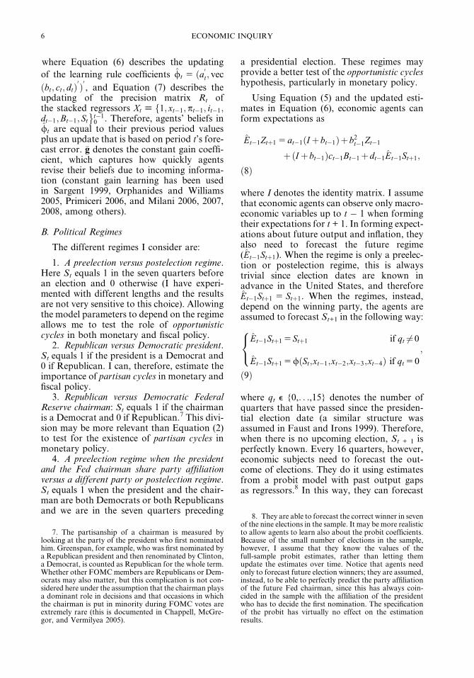
3. Republican versus Democratic FederalReserve chairman: St equals 1 if the chairmanis a Democrat and 0 if Republican.7 This divi-sion may be more relevant than Equation (2)to test for the existence of partisan cycles inmonetary policy.

4. A preelection regime when the presidentand the Fed chairman share party affiliationversus a different party or postelection regime.St equals 1 when the president and the chair-man are both Democrats or both Republicansand we are in the seven quarters preceding

a presidential election. These regimes mayprovide a better test of the opportunistic cycleshypothesis, particularly in monetary policy.

Using Equation (5) and the updated esti-mates in Equation (6), economic agents canform expectations as

Et�1Ztþ1 5 at�1ðIþbt�1Þþb2t�1Zt�1

þðIþbt�1Þct�1Bt�1þdt�1Et�1Stþ1;

ð8Þ

where I denotes the identity matrix. I assumethat economic agents can observe only macro-economic variables up to t � 1 when formingtheir expectations for t + 1. In forming expect-ations about future output and inflation, theyalso need to forecast the future regime(Et�1Stþ1). When the regime is only a preelec-tion or postelection regime, this is alwaystrivial since election dates are known inadvance in the United States, and thereforeEt�1Stþ1 5 Stþ1. When the regimes, instead,depend on the winning party, the agents areassumed to forecast St+1 in the following way:

Et�1Stþ15Stþ1 if qt 6¼0

Et�1Stþ15/ðSt;xt�1;xt�2;xt�3;xt�4Þ if qt50

;

8<:ð9Þ

where qt e {0,. . .,15} denotes the number ofquarters that have passed since the presiden-tial election date (a similar structure wasassumed in Faust and Irons 1999). Therefore,when there is no upcoming election, St + 1 isperfectly known. Every 16 quarters, however,economic subjects need to forecast the out-come of elections. They do it using estimatesfrom a probit model with past output gapsas regressors.8 In this way, they can forecast

7. The partisanship of a chairman is measured bylooking at the party of the president who first nominatedhim. Greenspan, for example, who was first nominated bya Republican president and then renominated by Clinton,a Democrat, is counted as Republican for the whole term.Whether other FOMC members are Republicans or Dem-ocrats may also matter, but this complication is not con-sidered here under the assumption that the chairman playsa dominant role in decisions and that occasions in whichthe chairman is put in minority during FOMC votes areextremely rare (this is documented in Chappell, McGre-gor, and Vermilyea 2005).

8. They are able to forecast the correct winner in sevenof the nine elections in the sample. It may be more realisticto allow agents to learn also about the probit coefficients.Because of the small number of elections in the sample,however, I assume that they know the values of thefull-sample probit estimates, rather than letting themupdate the estimates over time. Notice that agents needonly to forecast future election winners; they are assumed,instead, to be able to perfectly predict the party affiliationof the future Fed chairman, since this has always coin-cided in the sample with the affiliation of the presidentwho has to decide the first nomination. The specificationof the probit has virtually no effect on the estimationresults.

6 ECONOMIC INQUIRY

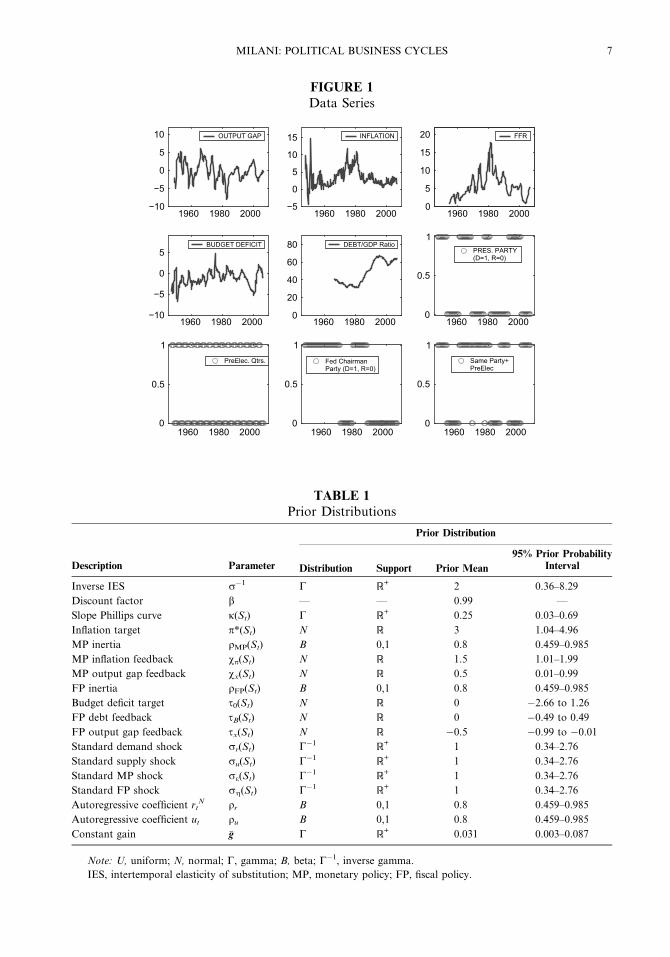
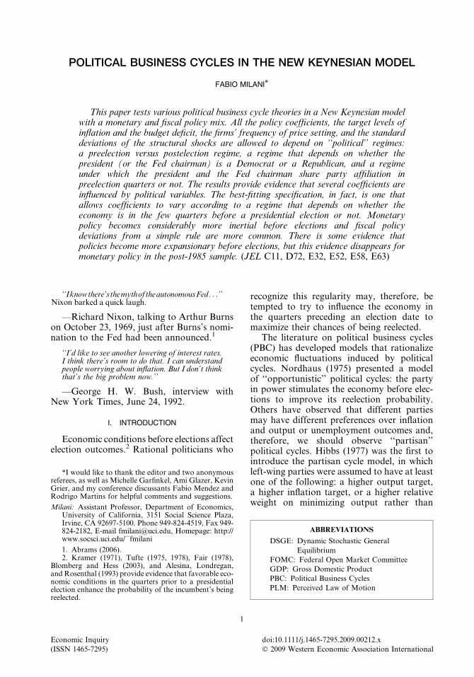
FIGURE 1

Data Series

1960 1980 2000−10

−5

0

5

10 OUTPUT GAP

1960 1980 2000−5

0

5

10

15 INFLATION

1960 1980 20000

5

10

15

20 FFR

1960 1980 2000−10

−5

0

5BUDGET DEFICIT

1960 1980 20000

20

40

60

80 DEBT/GDP Ratio

1960 1980 20000

0.5

1PRES. PARTY (D=1, R=0)

1960 1980 20000

0.5

1PreElec. Qtrs.

1960 1980 20000

0.5

1Fed ChairmanParty (D=1, R=0)

1960 1980 20000

0.5

1Same Party+ PreElec

TABLE 1

Prior Distributions

Description Parameter

Prior Distribution

Distribution Support Prior Mean

95% Prior ProbabilityInterval

Inverse IES r�1 C R+ 2 0.36–8.29

Discount factor b — — 0.99 —

Slope Phillips curve j(St) C R+ 0.25 0.03–0.69

Inflation target p*(St) N R 3 1.04–4.96

MP inertia qMP(St) B 0,1 0.8 0.459–0.985

MP inflation feedback vp(St) N R 1.5 1.01–1.99

MP output gap feedback vx(St) N R 0.5 0.01–0.99

FP inertia qFP(St) B 0,1 0.8 0.459–0.985

Budget deficit target s0(St) N R 0 �2.66 to 1.26

FP debt feedback sB(St) N R 0 �0.49 to 0.49

FP output gap feedback sx(St) N R �0.5 �0.99 to �0.01

Standard demand shock rr(St) C�1R

+ 1 0.34–2.76

Standard supply shock ru(St) C�1R

+ 1 0.34–2.76

Standard MP shock re(St) C�1R

+ 1 0.34–2.76

Standard FP shock rg(St) C�1R

+ 1 0.34–2.76

Autoregressive coefficient rtN qr B 0,1 0.8 0.459–0.985

Autoregressive coefficient ut qu B 0,1 0.8 0.459–0.985

Constant gain �g C R+ 0.031 0.003–0.087

Note: U, uniform; N, normal; C, gamma; B, beta; C�1, inverse gamma.

IES, intertemporal elasticity of substitution; MP, monetary policy; FP, fiscal policy.


the probability that the incumbent will wintheelectionsgiventhepastrelationbetweenelec-tion outcomes and macroeconomic conditions.

Therefore, the formation of expectations,as characterized in Equation (8), may differaccording to the political cycle. Agents maylearn from experience whether political varia-bles matter or not.

III. BAYESIAN ESTIMATION

I estimate the model by likelihood-basedBayesian methods.9 The Bayesian approachfacilitates the estimation of the learningparameters jointly with the structural param-eters of the economy. In particular, here I esti-mate the constant gain coefficient jointly with

the parameters describing preferences and themonetary and fiscal policy rule parameters.10

Milani (2007) shows that learning improvesthe empirical fit of a similar New Keynesianmodel compared with the rational expecta-tions case and it allows researchers to avoidincluding some of the so-called ‘‘mechanical’’sources of persistence that are needed to makethe model match the sluggishness of macro-economic variables.

I use quarterly U.S. data on inflation, out-put gap, the federal funds rate, the budget bal-ance, and the debt to GDP ratio. Inflation iscalculated as the log change in the GDPimplicit price deflator converted at annualrates, and the output gap as the log deviation

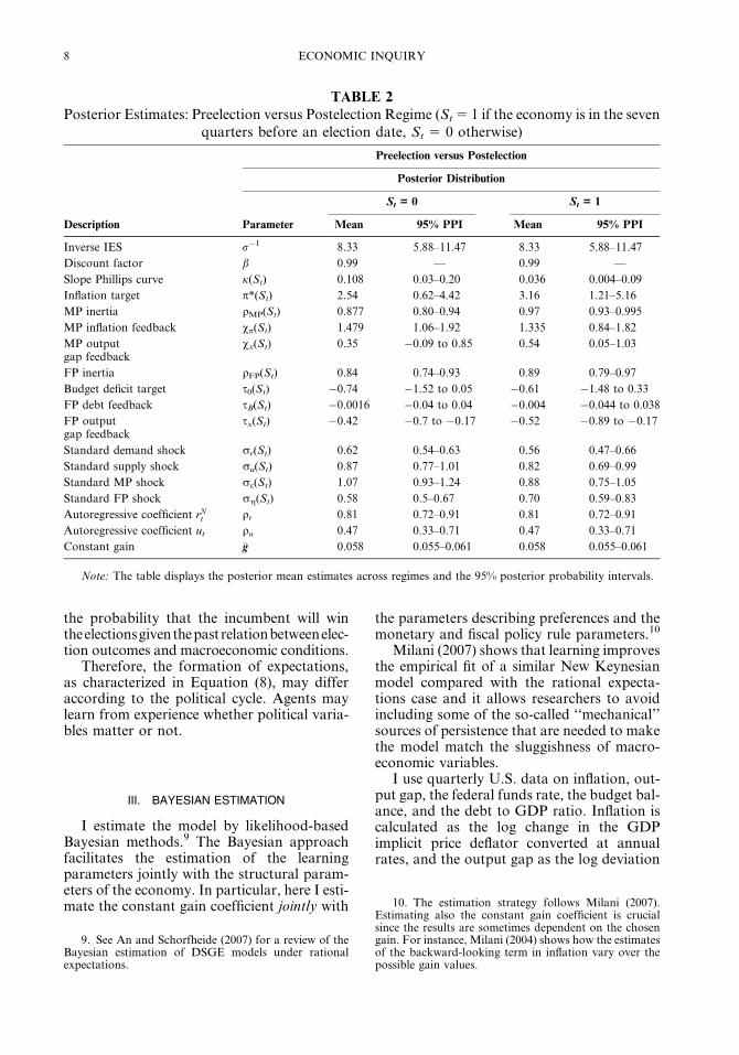
TABLE 2

Posterior Estimates: Preelection versus Postelection Regime (St5 1 if the economy is in the seven

quarters before an election date, St 5 0 otherwise)

Description

Preelection versus Postelection

Posterior Distribution

Parameter

St = 0 St = 1

Mean 95% PPI Mean 95% PPI

Inverse IES r�1 8.33 5.88–11.47 8.33 5.88–11.47

Discount factor b 0.99 — 0.99 —

Slope Phillips curve j(St) 0.108 0.03–0.20 0.036 0.004–0.09

Inflation target p*(St) 2.54 0.62–4.42 3.16 1.21–5.16

MP inertia qMP(St) 0.877 0.80–0.94 0.97 0.93–0.995

MP inflation feedback vp(St) 1.479 1.06–1.92 1.335 0.84–1.82

MP outputgap feedback

vx(St) 0.35 �0.09 to 0.85 0.54 0.05–1.03

FP inertia qFP(St) 0.84 0.74–0.93 0.89 0.79–0.97

Budget deficit target s0(St) �0.74 �1.52 to 0.05 �0.61 �1.48 to 0.33

FP debt feedback sB(St) �0.0016 �0.04 to 0.04 �0.004 �0.044 to 0.038

FP outputgap feedback

sx(St) �0.42 �0.7 to �0.17 �0.52 �0.89 to �0.17

Standard demand shock rr(St) 0.62 0.54–0.63 0.56 0.47–0.66

Standard supply shock ru(St) 0.87 0.77–1.01 0.82 0.69–0.99

Standard MP shock re(St) 1.07 0.93–1.24 0.88 0.75–1.05

Standard FP shock rg(St) 0.58 0.5–0.67 0.70 0.59–0.83

Autoregressive coefficient rNt qr 0.81 0.72–0.91 0.81 0.72–0.91

Autoregressive coefficient ut qu 0.47 0.33–0.71 0.47 0.33–0.71

Constant gain �g 0.058 0.055–0.061 0.058 0.055–0.061

Note: The table displays the posterior mean estimates across regimes and the 95% posterior probability intervals.

9. See An and Schorfheide (2007) for a review of theBayesian estimation of DSGE models under rationalexpectations.

10. The estimation strategy follows Milani (2007).Estimating also the constant gain coefficient is crucialsince the results are sometimes dependent on the chosengain. For instance, Milani (2004) shows how the estimatesof the backward-looking term in inflation vary over thepossible gain values.

8 ECONOMIC INQUIRY

of real GDP from potential GDP (using theseries computed by the Congressional BudgetOffice). The federal funds rate represents themonetary policy instrument, while the fiscalpolicy instrument is assumed to be the budgetdeficit, which is computed as federal govern-ment current expenditures minus interest pay-ments and minus federal government currentreceipts as a fraction of GDP. Bt in the modelis given by the debt to GDP ratio. The data areshown in Figure 1. All data series were down-loaded from FRED, the economic database ofthe Federal Reserve of St. Louis, and aredemeaned before the estimation.

The model coefficients are collected in thevector h:

hðStÞ5fr;p*ðStÞ;jðStÞ;qMPðStÞ;vpðStÞ;

vxðStÞ;qFPðStÞ;s0ðStÞ;sBðStÞ;sxðStÞ;

QðStÞ; �gg;

ð10Þ

where Q(St) groups the regime-dependentstandard deviations of the supply, demand,and policy shocks. The parameters dependon the political regime:

hðStÞ 5 h0ð1� StÞ þ h1ðStÞ;ð11Þ

where St corresponds to one of the regimesdiscussed in the previous section.

The learning process in Equations (6)and (7) needs to be initialized. The initial

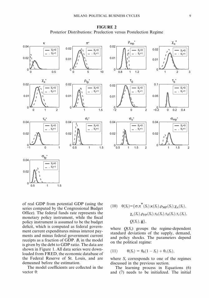
FIGURE 2

Posterior Distributions: Preelection versus Postelection Regime

0 0.50

0.02

0.04κ

St=0St=1

0 5 100

0.01

0.02

π*

0.8 1 1.20

0.01

0.02ρmp*

1 2 30

0.01

0.02

χπ*

0 1 20

0.01

0.02χx*

1 1.50

0.01

0.02ρfp*

−2 0 20

0.01

0.02

τ0

−0.2 0 0.2 0.40

0.05

0.1τb*

−1 0 10

0.02

0.04τx*

0.5 1 1.50

0.02

0.04σr*

0.5 1 1.5 20

0.02

0.04σu*

1 1.5 20

0.02

0.04σmp*

0.5 1 1.50

0.02

0.04σfp*

St=0St=1

St=0St=1

St=0St=1

St=0St=1

St=0St=1

St=0St=1

St=0St=1

St=0St=1

St=0St=1

St=0St=1

St=0St=1

St=0St=1


beliefs /0 and R0 are derived from estimatingthe PLM (Equation 5) on presample data(using observations from 1954:III to 1965:IV).

The model is then estimated using datafrom 1966:I to 2006:IV. The likelihood iscomputed for the four endogenous variables:inflation, output gap, federal funds rate, andbudget deficit.

I use the Metropolis-Hastings algorithm togenerate draws from the posterior distribu-tion. At each iteration, the likelihood is eval-uated using the Kalman filter. I consider300,000 draws, discarding an initial burn-inof 75,000 draws.

Table 1 describes the priors. I fix b equal to0.99. I assume a gamma distribution withmean 2 for r�1. The slope coefficient of thePhillips curve, j, follows a normal distributionwith mean 0.2 and standard deviation 0.1. Themonetary policy rule coefficients also follownormal distributions with mean 1.5 and stan-dard deviation 0.25 for the inflation feedbackcoefficients, and mean 0.5 and standard devi-ation 0.25 for the output feedback coefficients.

I choose inverse gamma distributions for thestandard deviations of the shocks and beta dis-tributions for the autoregressive coefficients.Finally, the constant gain coefficient followsa gamma distribution with prior mean 0.031and prior standard deviation 0.022.

I will emphasize in describing the results thecases in which the likelihood seems flat forsome of the parameters and those for whichthe priors appear to have a strong influenceon the shape of the posterior.11

IV. RESULTS

A. Opportunistic Cycles in Fiscal andMonetaryPolicies

I start by testing for the existence of oppor-tunistic cycles. These can manifest themselves

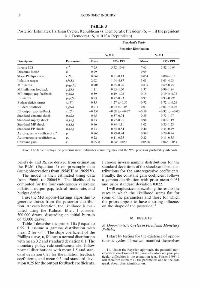
TABLE 3

Posterior Estimates: Partisan Cycles, Republican vs. Democratic President (St5 1 if the president

is a Democrat, St 5 0 if a Republican)


President’s Party


St = 0 St = 1


Inverse IES r–1 7.65 5.42–10.64 7.65 5.42–10.64




MP inertia qMP(St) 0.906 0.85–0.96 0.837 0.69–0.95


MP output gap feedback vx(St) 0.59 0.19–1.02 0.19 �0.19 to 0.73

FP inertia qFP(St) 0.83 0.72–0.93 0.97 0.93–0.995

Budget deficit target s0(St) �0.35 �1.27 to 0.56 �0.72 �1.72 to 0.26

FP debt feedback sB(St) 0.014 �0.02 to 0.05 0.03 �0.01 to 0.07

FP output gap feedback sx(St) �0.357 �0.68 to �0.07 �0.50 �0.92 to �0.05





Autoregressive coefficient rtN qr 0.865 0.79–0.94 0.865 0.79–0.94


Constant gain �g 0.0508 0.048–0.053 0.0508 0.048–0.053


11. Under the Bayesian approach, the potential non-identification of some of the parameters does not pose par-ticular difficulties in the estimation (e.g., Poirier 1998). Iwill therefore estimate all the parameters and let the dataspeak about their identification.

10 ECONOMIC INQUIRY

as an overstimulation of the economy duringthe quarters preceding an election.

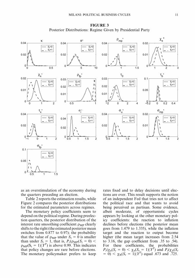
Table 2 reports the estimation results, whileFigure 2 compares the posterior distributionsfor the estimated parameters across regimes.

The monetary policy coefficients seem todepend on the political regime. During preelec-tion quarters, the posterior distribution of theinterest rate smoothing coefficient qMP clearlyshifts to the right (the estimated posterior meanswitches from 0.877 to 0.97); the probabilitythat the value of qMP under St 5 0 is smallerthan under St 5 1, that is, Pr(qMP(St 5 0) ,qMP(St 5 1)jYT) is above 0.99. This indicatesthat policy changes are rare before elections.The monetary policymaker prefers to keep

rates fixed and to delay decisions until elec-tions are over. This result supports the notionof an independent Fed that tries not to affectthe political race and that wants to avoidbeing perceived as partisan. Some evidence,albeit moderate, of opportunistic cyclesappears by looking at the other monetary pol-icy coefficients: the reaction to inflationdeclines before elections (the posterior meangoes from 1.479 to 1.335), while the inflationtarget and the reaction to output becomehigher (the mean target increases from 2.54to 3.16, the gap coefficient from .35 to .54).For these coefficients, the probabilitiesPr(vp(St 5 0) , vp(St 5 1)jYT) and Pr(vX(St

5 0) , vX(St 5 1)jYT) equal .673 and .725.

FIGURE 3

Posterior Distributions: Regime Given by Presidential Party

0 0.50

0.02

0.04κ

St=0St=1

5 100

0.02

0.04π*

St=0St=1

1 1.50

0.02

0.04ρmp*

St=0St=1

1 2 30

0.01

0.02χπ*

St=0St=1

0 1 20

0.01

0.02χx*

St=0St=1

0.5 10

0.01

0.02

0.03

ρfp*

St=0St=1

−2 0 2 40

0.01

0.02

0.03τ0

St=0St=1

−0.2 0 0.2 0.40

0.05

0.1τb*

St=0St=1

−1 0 1 20

0.02

0.04τx*

St=0St=1

0.5 1 1.5 20

0.02

0.04

σr*

St=0St=1

0.5 1 1.5 20

0.02

0.04σu*

St=0St=1

1 1.5 20

0.01

0.02σmp*

St=0St=1

0.5 1 1.50

0.05

0.1σfp*

St=0St=1


Fiscal policy is likewise more inertial beforeelections (the posterior mean for qFP is 0.89 inpreelection quarters, 0.84 otherwise) and thetarget deficit higher before elections. The stan-dard deviations of both monetary and fiscalpolicy surprises are strongly affected by theproximity of an election: fiscal policy devia-tions from the rule are considerably morecommon and sizeable before elections (theposterior distribution shifts to the right), whilemonetary policy deviations are less so (since,as seen, monetary policy decisions are unlikelyin this regime).

Finally, another parameter that is cruciallyaffected by the proximity to an election is j,which denotes the slope of the Phillips curveand is an inverse function of the degree of pricerigidity in the economy. The distribution of jtilts toward 0 when St5 1, signaling that firmstend to have higher probability to keep pricesfixed in the quarters before elections (for j, theprobability Pr(j(St 5 0) , j(St 5 1)jYT)equals 0.95). From the estimated j, we can

derive the implied Calvo parameter a, suchthat (1 � a) denotes the probability of firms’changing prices in a given quarter (or equiva-lently, the fraction of firms that change pricesin a given quarter). (1 � a) goes from 0.28 inafter-election quarters to 0.17 right beforeelections.12 Therefore, firms prefer to delaythe price-setting decision until the electoraluncertainty is resolved.13

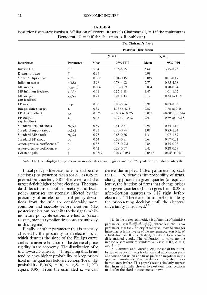
TABLE 4

Posterior Estimates: Partisan Affiliation of Federal Reserve’s Chairman (St5 1 if the chairman is

Democrat, St 5 0 if the chairman is Republican)


Fed Chairman’s Party


St = 0 St = 1


Inverse IES r–1 5.64 3.75–8.25 5.64 3.75–8.25




MP inertia qMP(St) 0.904 0.78–0.99 0.834 0.70–0.94



vx(St) 0.71 0.24–1.13 0.12 �0.34 to 1.65

FP inertia qFP 0.90 0.83–0.96 0.90 0.83–0.96

Budget deficit target s0 �0.82 �1.78 to 0.15 �0.82 �1.78 to 0.15

FP debt feedback sB 0.035 �0.005 to 0.074 0.035 �0.005 to 0.074


sx �0.47 �0.79 to �0.18 �0.47 �0.79 to �0.18




Standard FP shock rg 0.64 0.57–0.71 0.64 0.57–0.71

Autoregressive coefficient rtN qr 0.85 0.75–0.931 0.85 0.75–0.93


Constant gain �g 0.0517 0.048–0.054 0.0517 0.048–0.054


12. In the presented model, j is a function of primitive

parameters, j [ð1�aÞð1�abÞ

aðxþr�1Þ1þxh , where a is the Calvo

parameter, x is the elasticity of marginal costs to changesin income, r is the inverse of the intertemporal elasticity ofsubstitution, and h is the elasticity of substitution betweendifferentiated goods. The calibration to calculate theimplied a here assumes standard values: x 5 0.8, r 5 1,and h 5 7.

13. Garfinkel and Glazer (1994) looked at the distri-bution of wage contracts in election and nonelection yearsand found that union and firms prefer to negotiate in thequarters immediately after the election rather than thoseimmediately before. This paper’s results similarly suggestthat firms rationally choose to postpone their decisionuntil after the election outcome is known.

12 ECONOMIC INQUIRY

B. Partisan Cycles in Fiscal and MonetaryPolicies

Economic parameters and policies may sys-tematically differ depending on whethera Republican or Democratic president is inthe White House. Table 3 and Figure 3 pro-vide evidence on this hypothesis. Again themonetary and fiscal policy parameters differacross political regimes, although in a waythat seems to contradict the theory. Monetarypolicy is more inertial during Republicanterms; the feedback coefficient to inflation ishigher and the feedback to the output gaplower under Democrats than under Republi-cans.14 This is the opposite of what is usuallytheorized by PBC studies (and of what wasfound by Fang and Jeliazkov 2007). The pos-

terior distributions of monetary policy param-eters during Republican presidencies are alsosuch that a nontrivial probability mass refersto policies that do not respect the Taylor prin-ciple.15 Fiscal policy also displays a higher tar-get for the budget deficit and a lower reactionto changes in the output gap under Republi-can presidents than under Democrats (fiscalpolicy with Democratic presidents is consider-ably inertial, instead).16 Turning to other para-meters, the demand and supply shocks that

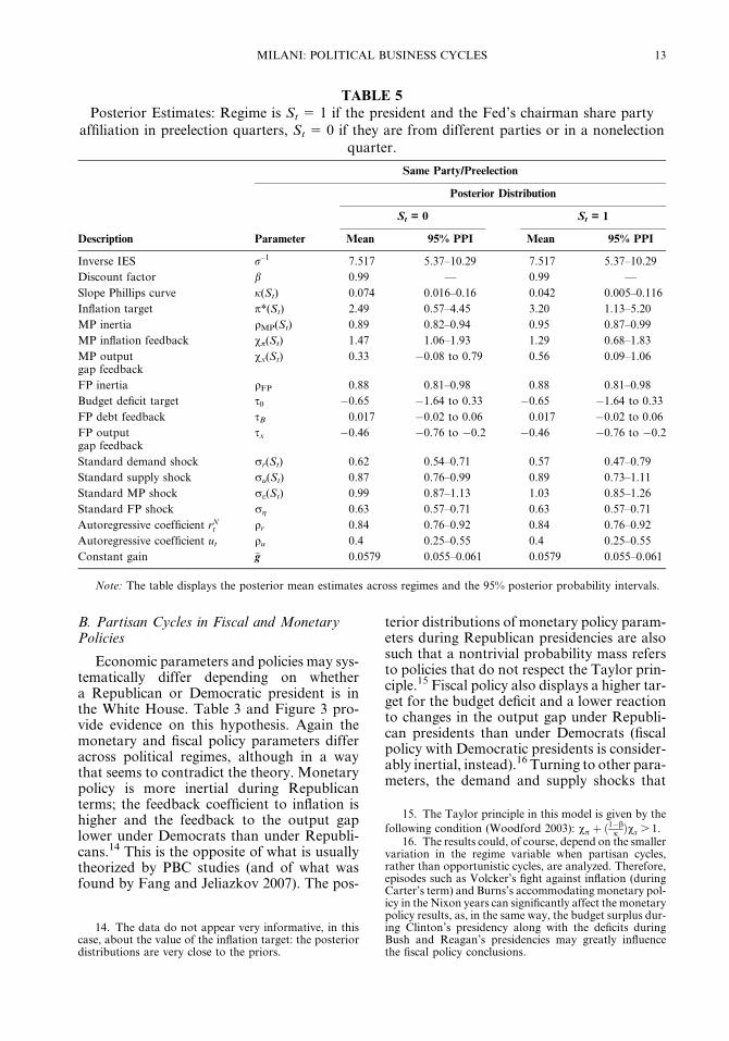
TABLE 5

Posterior Estimates: Regime is St 5 1 if the president and the Fed’s chairman share party

affiliation in preelection quarters, St 5 0 if they are from different parties or in a nonelection

quarter.

Description

Same Party/Preelection


St = 0 St = 1

Parameter Mean 95% PPI Mean 95% PPI

Inverse IES r–1 7.517 5.37–10.29 7.517 5.37–10.29




MP inertia qMP(St) 0.89 0.82–0.94 0.95 0.87–0.99



vx(St) 0.33 �0.08 to 0.79 0.56 0.09–1.06

FP inertia qFP 0.88 0.81–0.98 0.88 0.81–0.98

Budget deficit target s0 �0.65 �1.64 to 0.33 �0.65 �1.64 to 0.33

FP debt feedback sB 0.017 �0.02 to 0.06 0.017 �0.02 to 0.06


sx �0.46 �0.76 to �0.2 �0.46 �0.76 to �0.2




Standard FP shock rg 0.63 0.57–0.71 0.63 0.57–0.71



Constant gain �g 0.0579 0.055–0.061 0.0579 0.055–0.061


14. The data do not appear very informative, in thiscase, about the value of the inflation target: the posteriordistributions are very close to the priors.

15. The Taylor principle in this model is given by the

following condition (Woodford 2003): vp þ ð1�bj Þvx . 1.

16. The results could, of course, depend on the smallervariation in the regime variable when partisan cycles,rather than opportunistic cycles, are analyzed. Therefore,episodes such as Volcker’s fight against inflation (duringCarter’s term) and Burns’s accommodating monetary pol-icy in the Nixon years can significantly affect the monetarypolicy results, as, in the same way, the budget surplus dur-ing Clinton’s presidency along with the deficits duringBush and Reagan’s presidencies may greatly influencethe fiscal policy conclusions.


have hit the economy had higher standarddeviation during Democratic terms.

C. Partisan Cycles Using Fed Chairman’sAffiliation

Since the Federal Reserve has full indepen-dence in setting monetary policy, the party’saffiliation or sympathy of the Fed chairmancould, in principle, be more relevant thanthe president’s party to test for partisan differ-ences in monetary policy.

The estimation results (shown in Table 4),however, mirror those in the previous section.Fed chairmen that were appointed by Demo-cratic presidents have on average reacted moreaggressively toward inflation and worried lessabout output fluctuations compared withthose appointed by Republican presidents. Itshould be emphasized, however, that onlya few changes in the relevant political variableare available in the sample and, therefore, theresults are likely to depend a lot on ArthurBurns’s passive monetary policy (which is

counted as Republican) and Paul Volcker’saggressive policy during the disinflation(which affects the results for Democrats).

D. Opportunistic Cycles in Monetary PolicyWhen the President and the Fed ChairmanShare Party Affiliation

It may be realistic to argue that opportunis-tic cycles are present only when the Fed chair-man shares political party with the president.Abrams and Iossifov (2006), in fact, find thatthis is the only case in which political cyclesmatter in their estimated Taylor rules. Alongthe same lines, Chappell, McGregor, andVermilyea (2005), analyzing Federal OpenMarket Committee (FOMC) voting records,show that FOMC members are more likelyto support a preelection expansionary mone-tary policy when they were appointed bya president of the incumbent party.

The evidence, presented in Table 5, is similarto that on opportunistic cycles. Monetary pol-icy is especially inertial before elections even

TABLE 6

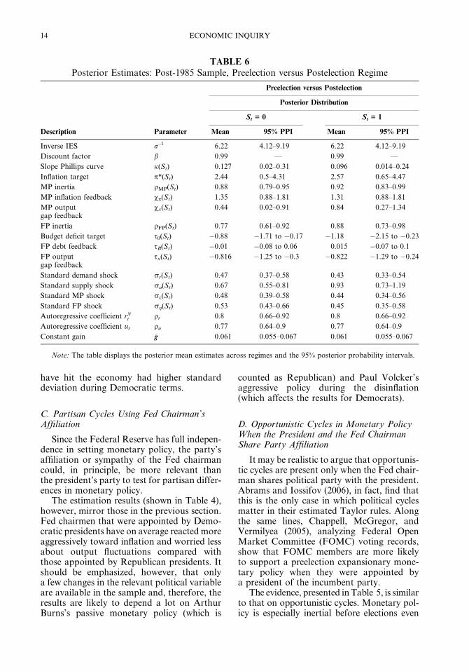
Posterior Estimates: Post-1985 Sample, Preelection versus Postelection Regime


Preelection versus Postelection


St = 0 St = 1


Inverse IES r–1 6.22 4.12–9.19 6.22 4.12–9.19




MP inertia qMP(St) 0.88 0.79–0.95 0.92 0.83–0.99



vx(St) 0.44 0.02–0.91 0.84 0.27–1.34

FP inertia qFP(St) 0.77 0.61–0.92 0.88 0.73–0.98

Budget deficit target s0(St) �0.88 �1.71 to �0.17 �1.18 �2.15 to �0.23

FP debt feedback sB(St) �0.01 �0.08 to 0.06 0.015 �0.07 to 0.1


sx(St) �0.816 �1.25 to �0.3 �0.822 �1.29 to �0.24







Constant gain �g 0.061 0.055–0.067 0.061 0.055–0.067


14 ECONOMIC INQUIRY

when the president and the Fed chairman havesimilar political sympathies. There is evidenceof a lower reaction toward inflation, a higherinflation target, and a larger reaction tochanges in the output gap before elections.

E. Beliefs

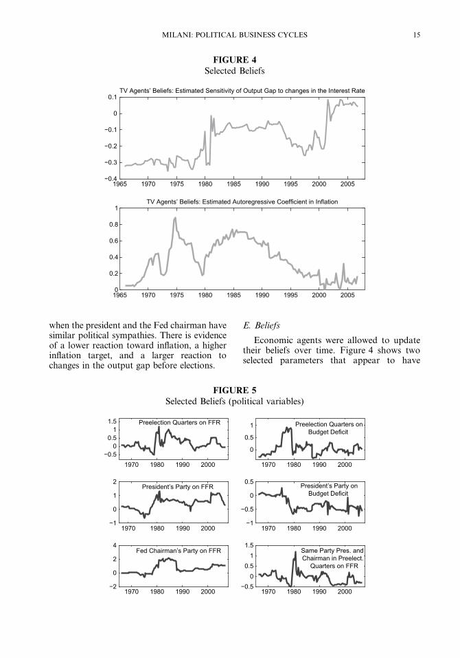
Economic agents were allowed to updatetheir beliefs over time. Figure 4 shows twoselected parameters that appear to have

FIGURE 4

Selected Beliefs

1965 1970 1975 1980 1985 1990 1995 2000 2005−0.4

−0.3

−0.2

−0.1

0

0.1TV Agents’ Beliefs: Estimated Sensitivity of Output Gap to changes in the Interest Rate

1965 1970 1975 1980 1985 1990 1995 2000 20050

0.2

0.4

0.6

0.8

1TV Agents’ Beliefs: Estimated Autoregressive Coefficient in Inflation

FIGURE 5

Selected Beliefs (political variables)

1970 1980 1990 2000−1

0

1

2President’s Party on FFR

1970 1980 1990 2000−1

−0.5

0

0.5 President’s Party onBudget Deficit

1970 1980 1990 2000−0.5

00.5

11.5 Preelection Quarters on FFR

1970 1980 1990 2000

0

0.5

1 Preelection Quarters onBudget Deficit

1970 1980 1990 2000−2

0

2

4Fed Chairman’s Party on FFR

1970 1980 1990 2000−0.5

00.5

11.5

Same Party Pres. andChairman in Preelect.

Quarters on FFR


considerably changed over the sample. One isthe perceived sensitivity of the output gap tochanges in the interest rate. Agents’ beliefsevolve over the sample to reflect the perceptionof declining sensitivity. The second is theautoregressive coefficient in the PLM for infla-tion, which indicates changes in the perceivedpersistence of this variable. The estimatedcoefficient starts at values close to 0, but it con-siderably increases from the late 1960s to theearly 1970s and later in the 1980s, to declineagain to low values at the end of the sample.Adding learning to the model admits thisimportant time variation in beliefs, whichwould be ruled out under rational expectations.

Figure 5, instead, shows the evolvingagents’ beliefs about the importance of the dif-ferent political variables. For example, look-ing at the first row in the graph, it can beseen that agents adjust their beliefs in the1970s as they are learning that policy ratesare lower and the budget deficit higher beforeelections. During Carter’s term, though, thesebeliefs are quickly revised. In a way that isconsistent with the model estimates, agents

perceive more contractionary monetary andfiscal policies during Democratic terms.

F. Model Comparison

To assess which model provides the best fitof the data, I compare the models’ marginallikelihoods using Geweke’s modified har-monic mean approximation. The marginallikelihoods favor the opportunistic cyclesmodel (the log marginal likelihood equals�785.67). The opportunistic cycle when thepresident and the Fed chairman come fromthe same party ranks second (�790.83). Ofcourse, partisan cycles may also be present—Isimply find that, as a single explanation, theyfit less well than opportunistic cycles—but thelimited data do not allow including more thanone regime at a time in the model. Partisancycles may also suffer from a lower variabilityof the regime over the sample.17

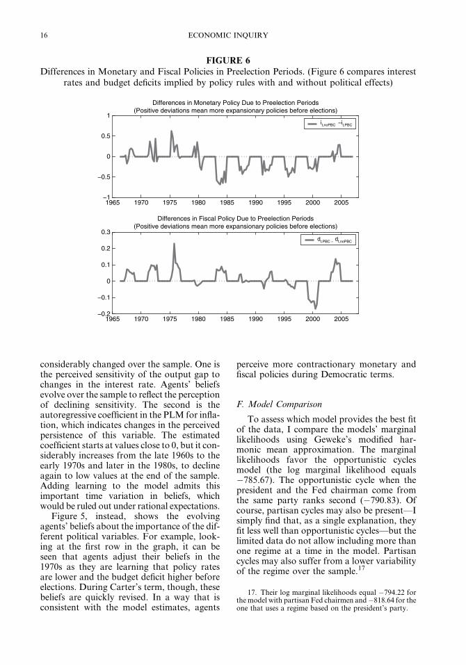
FIGURE 6

Differences in Monetary and Fiscal Policies in Preelection Periods. (Figure 6 compares interestrates and budget deficits implied by policy rules with and without political effects)

1965 1970 1975 1980 1985 1990 1995 2000 2005−1

−0.5

0

0.5

1

Differences in Monetary Policy Due to Preelection Periods(Positive deviations mean more expansionary policies before elections)

it,noPBC −it,PBC

1965 1970 1975 1980 1985 1990 1995 2000 2005−0.2

−0.1

0

0.1

0.2

0.3

Differences in Fiscal Policy Due to Preelection Periods(Positive deviations mean more expansionary policies before elections)

dt,PBC − dt,noPBC

17. Their log marginal likelihoods equal �794.22 forthe model with partisan Fed chairmen and �818.64 for theone that uses a regime based on the president’s party.

16 ECONOMIC INQUIRY

Allowing coefficients to depend on thepolitical regime can improve the model fit.Although the traditional New Keynesianmodel with no political variables fits betterthan the model in which almost all coefficientsdepend on the political regime (the log mar-ginal likelihood equals �777.62 vs. �785.67),it is outperformed by more parsimonious mod-els that assume that politics affects only a subsetof coefficients, as for example the one in whichonly the monetary and fiscal policy inertia coef-ficients, qMP(St) and qFP(St), and the standarddeviations of policy shocks, re(St) and rg(St),are regime dependent (the log marginal likeli-hood in this case, in fact, increases to �776.93).

G. What Would Monetary and Fiscal PolicyHave Been in the Absence of Political Effects?

Under opportunistic cycles, which is thecase that is most supported by the data, themonetary and fiscal policy rules differ in pre-election versus postelection quarters. But howlarge are the differences in practice?

Figure 6 displays the deviations in the mon-etary and fiscal policy instruments that arefound by comparing the implied FederalFunds rate and budget deficit obtained byusing the same policy rules that are estimatedfor nonelection quarters for the whole samplewith those implied by rules that differ, asestimated, in preelection quarters. The graph

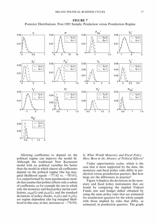
FIGURE 7

Posterior Distributions: Post-1985 Sample, Preelection versus Postelection Regime

0 0.5 10

0.01

0.02κ

0 5 10 15

π*

St=0St=1

1 1.50

0.01

0.02

ρmp

*

St=0St=1

1 2 30

0.01

0.02χπ*

St=0St=1

0 2 40

0.01

0.02

χx*

St=0St=1

1 1.5

ρfp

*

St=0St=1

−2 0 2 40

0.01

0.02

0.03τ0

St=0St=1

0 0.2 0.40

0.02

0.04

0.06τ

b*

St=0St=1

−1 0 10

0.01

0.02τx*

St=0St=1

0.5 1 1.5

0

0.01

0.02

0

0.01

0.02

0

0.02

0.04

σr*

St=0St=1

0.5 1 1.5 20

0.02

0.04σu*

St=0St=1

0.5 1 1.50

0.02

0.04σmp*

St=0St=1

0.5 1 1.5 20

0.02

0.04

σfp*

St=0St=1


shows that monetary policy has typically beenmore expansionary before elections in the pre-1979 sample, but after Volcker, the increasedinertia seems to have led the central bank tobe, instead, more contractionary, except inthe later part of the sample. Fiscal policyhas been consistently more expansionarybefore elections, with the main exceptionbeing during the Clinton years.

H. Post-1985 Sample

I repeat the estimation on data starting from1985:I. Monetary policy is still considerablymore inertial before elections, and so is fiscalpolicy (Table 6 and Figure 7). There is no evi-dence that monetary policy reacts differently toinflation in the proximity of elections: the infla-tion target and inflation feedback coefficient arecharacterized by posterior distributions thatsubstantiallyoverlap.Thereaction totheoutputgap is slightly larger before elections.

V. CONCLUSIONS

This paper has tested whether the coeffi-cients of a baseline New Keynesian modeldepend on political variables. The paper hasprovided empirical evidence on PBC theories,testing different versions of both opportunisticand partisan cycle models.

The results provide some support for theexistence of changes in the economic structureand policies that are due to political variables.The best-fitting model is one that allows policyand structural parameters to depend onwhether the economy is or is not in preelectionquarters, as in opportunistic cycles’ models.The results, however, are not entirely consis-tent with opportunistic cycles as they are usu-ally interpreted.

The major difference in preelection quar-ters is that monetary policy becomes consider-ably more inertial: the Fed seems to delaychanges in policy until after the election. Thisis consistent with the view of an independentFed, which does not want to be seen as anactive player in the presidential race. Some evi-dence, however, exists that both monetary(before Volcker) and fiscal policies have beensomewhat less concerned about inflation andmore about output before elections.

As a future avenue for research, it may beworthwhile testing for electoral effects in fiscal

policy at a lower level of aggregation. In thispaper, the fiscal policy instrument has beenconsidered to be the budget deficit. But futurework may fruitfully test whether political var-iables matter more for government spendingor for average tax rates, and, regarding spend-ing, for which categories of governmentspending in particular. Likewise, futureresearch should investigate whether thechange in policies before elections displaysasymmetries across recessions and expansionsor periods of rising versus falling inflation.

APPENDIX: METROPOLIS-HASTINGS ALGORITHM

The information about the parameters is summarizedby the posterior distribution, obtained by Bayes theorem

pðhjYT Þ 5 pðYT jhÞpðhÞ;p YT

��ð12Þ

where p(YTjh) is the likelihood function, p(h) the prior forthe parameters, and YT 5 [y1,. . .,yT]# collects the data his-tories.

To generate draws from the posterior distributionp(hjYT), I use the Metropolis algorithm. The procedureworks as follows.

1. Start from an arbitrary value for the parametervector h0. Set j 5 1.

2. Evaluate p(YTjh0)p(h0).

3. Generate h*j 5 hj�1 þ e, where h*j is the proposaldraw and e ; N(0, cRe). c is a scale factor that is usuallyadjusted to keep the acceptance ratio of the MH algorithmat an optimal rate (25–50%). The acceptance rates in theestimation are all between 35 and 40%.

4. Generate u from a Uniform[0, 1].5. Set

hj 5 h*j if u� aðhj�1;h�j Þ5min

pðYT jh�j Þpðh*j ÞpðYT jhj�1Þpðhj�1Þ;1

� �

hj 5 hj�1 if u.aðhj�1;h*j Þ:

8><>:

6. Repeat for j + 1 from 2 until j 5 D (D 5 totalnumber of draws).

Convergence

To assess convergence of the Markov chain MonteCarlo simulation, I performed various checks, besideslooking at the trace plots of the draws. I have consideredthe convergence tests proposed by Geweke (1992) andRaftery and Lewis (1995). Raftery and Lewis’s (1995)diagnostics suggests a minimum number of total draws,a thinning parameter, and a minimum burn-in, by com-puting the autocorrelation of the draws. Geweke’s testinstead compares the partial means l1 5 1

D1

PD1

j 5 1 gðhjÞand l2 5 1

D2

PD2

j 5 D1þ1 gðhjÞ, obtained from the first D1

and last D2 simulation draws. The null hypothesis ofequal means between the two samples of draws canbe tested knowing that, for D/‘, the quantity

ðl1 � l2Þ=ðS1gð0ÞD1

þ S2gð0ÞD2

Þ1=20Nð0; 1Þ. I also look at the

18 ECONOMIC INQUIRY

plots derived from the test proposed by Yu and Mykland(1994), based on CUMSUM plots of the draws.18 Finally,I ascertain convergence by looking at the recursive meanplots and bivariate scatter plots among the parameters toevaluate the mixing of the chain.

REFERENCES

Abrams, B. A. ‘‘How Richard Nixon Pressured ArthurBurns: Evidence From the Nixon Tapes.’’ Journalof Economic Perspectives, 20(4), 2006, 177–88.

Abrams B. A., and P. Iossifov. ‘‘Does the Fed Contributeto the Political Business Cycle?’’ Public Choice, 129,2006, 249–62.

Adam, K. ‘‘Learning to Forecast and Cyclical Behavior ofOutput and Inflation.’’ Macroeconomic Dynamics, 9,2005, 1–27.

Alesina, A. ‘‘Macroeconomics and Politics,’’ inNBERMac-roeconomics Annual, edited by Stanley Fischer. Cam-bridge, MA: MIT Press, 1988, 17–52.

Alesina, A., G. Cohen, and N. Roubini. ‘‘MacroeconomicPolicy and Elections in OECD Democracies.’’ Eco-nomics and Politics, 4, 1992, 1–30.

Alesina, A., J. Londregan, and H. Rosenthal. ‘‘A Model ofthe Political Economy of the United States.’’ Amer-ican Political Science Review, 87, 1993, 12–33.

Alesina, A., N. Roubini, and G. Cohen.Political Cycles andtheMacroeconomy.Cambridge,MA:MITPress,1997.

An, S., and F. Schorfheide. ‘‘Bayesian Analysis of DSGEModels.’’ Econometric Reviews, 26, 2007, 113–72.

Beck, N. ‘‘Elections and the Fed: Is There a Political Mon-etary Cycle?’’ American Journal of Political Science,31, 1987, 194–216.

Blomberg, B. S., and G. D. Hess. ‘‘Is the Political BusinessCycle for Real?’’ Journal of Public Economics, 87,2003, 1091–121.

Chappell, E. W., R. R. McGregor, and T. Vermilyea.Committee Decisions on Monetary Policy: Evidencefrom Historical Records of the Federal Open MarketCommittee. Cambridge, MA: MIT Press, 2005.

Drazen, A. Political Economy in Macroeconomics. Prince-ton, NJ: Princeton University Press, 2000a.

Drazen, A. ‘‘The Political Business Cycle after 25 Years,’’in NBER Macroeconomics Annual, edited by Ben S.Bernanke and Kenneth Rogoff. Cambridge, MA:MIT Press. 2000b, 75–117.

Evans,G.W.,andS.Honkapohja.LearningandExpectationsin Macroeconomics. Princeton, NJ: Princeton Univer-sity Press, 2001.

Fair, R. ‘‘The Effect of Economic Events on Votes forPresident.’’ Review of Economics and Statistics, 60,1978, 159–72.

Fang, A., and I. Jeliazkov. Politics and MacroeconomicPerformance in the United States: Cycles andLong-Run Outcomes. Manuscript, University ofCalifornia, Irvine, 2007.

Faust, J., and J. Irons. ‘‘Money, Politics, and the Post-WarBusiness Cycle.’’ Journal ofMonetary Economics, 43,1999, 61–89.

Favero, C. A., and T. Monacelli.Monetary-FiscalMix andInflation Performance: Evidence from the U.S.Mimeo, IGIER–Bocconi University, 2005.

Garfinkel, M., and A. Glazer. ‘‘Does Electoral Uncer-tainty Cause Economic Fluctuations?’’ AmericanEconomic Review, 84, 1994, 169–73.

Grier,K.B.‘‘OntheExistenceofaPoliticalMonetaryCycle.’’American Journal ofPolitical Science, 33, 1989, 376–89.

Grier, K. B. Forthcoming. ‘‘Presidential Elections andReal GDP Growth in the USA, 1961–2004.’’ PublicChoice, 135, 2008, 337–52.

Hibbs, D. ‘‘Political Parties and Macroeconomic Policy.’’American Political Science Review, 71, 1977, 1467–87.

Honkapohja, S., K. Mitra, and G. W. Evans. ‘‘Notes onAgents’ Behavioral Rules Under Adaptive Learningand Recent Studies of Monetary Policy.’’ Manu-script, Cambridge University, University of St.Andrews, and University of Oregon, 2002.

Keech, W., and K. Pak. ‘‘Electoral Cycles and BudgetaryGrowth in Veterans’ Benefit Programs.’’ AmericanJournal of Political Science, 33, 1989, 901–11.

Kramer, G. H. ‘‘Short-Term Fluctuations in U.S. VotingBehavior, 1896-1964.’’ The American Political Sci-ence Review, 65, 1971, 131–43.

Krause, S., and F. Mendez. ‘‘Policy Makers’ Preferences,Party Ideology and the Political Business Cycle.’’Southern Economic Journal, 71, 2005, 752–67.

Milani, F. Adaptive Learning and Inflation Persistence.Mimeo, University of California, Irvine, 2004.

Milani, F. ‘‘A Bayesian DSGE Model with Infinite-Horizon Learning: Do "Mechanical" Sources of Per-sistence Become Superfluous?’’ International Journalof Central Banking, 2, 2006, 87–106.

Milani, F. ‘‘Expectations, Learning and MacroeconomicPersistence.’’ Journal of Monetary Economics, 54,2007, 2065–82.

Milani, F. ‘‘Learning, Monetary Policy Rules, and Mac-roeconomic Stability.’’ Journal of Economic, Dynam-ics, and Control, 32, 2008, 3148–65.

Muscatelli, A., P. Tirelli, and C. Trecroci. ‘‘Fiscal and Mon-etary Policy Interactions: Empirical Evidence andOptimal Policy Using a Structural New-KeynesianModel.’’Journal ofMacroeconomics, 26, 2004, 257–80.

Nordhaus, W. ‘‘The Political Business Cycle.’’ Review ofEconomic Studies, 42, 1975, 169–90.

Orphanides, A., and J. Williams. ‘‘The Decline of ActivistStabilization Policy: Natural Rate Misperceptions,Learning, and Expectations.’’ Journal of EconomicDynamics and Control, 29, 2005, 1927–50.

Poirier, D. ‘‘Revising Beliefs in Nonidentified Models.’’Econometric Theory, 14, 1998, 483–509.

Preston, B. ‘‘Learning About Monetary Policy RulesWhen Long-Horizon Expectations Matter.’’ Interna-tional Journal of Central Banking, 1, 2005, 81–126.

Primiceri, G. ‘‘Why Inflation Rose and Fell: Policy-makers’ Beliefs and Postwar Stabilization Policy.’’Quarterly Journal of Economics, 121, 2006, 867–901.

Raftery, A. E., and S. M. Lewis. ‘‘The Number of Itera-tions, Convergence Diagnostics, and GenericMetropolis Algorithms.’’ Practical Markov ChainMonte Carlo, edited by W. R. Gilks, D. J. Spiegelhal-ter, and S. Richardson. London: Chapman and Hall,1995.

Sargent, T. J. The Conquest of American Inflation. Prince-ton, NJ: Princeton University Press. 1999.

18. They propose the statistics CSt 5 ð1t

Ptd 5 1 h

dÞ�lh=rh, where lh and rh are the empirical mean and stan-dard deviations of the D draws of the Markov chain. Theplot of CSt converges to 0 as t increases.


Taylor, J. B. ‘‘Reassessing Discretionary Fiscal Policy.’’Journal of Economic Perspectives, 14(3), 2000, 21–36.

Tufte, E. ‘‘Determinants of the Outcomes of MidtermCongressional Elections.’’American Political ScienceReview, 69, 1975, 812–26.

Tufte, E. Political Control of the Economy, Princeton NJ:Princeton University Press, 1978.

Woodford, M. Interest and Prices: Foundations of aTheory ofMonetary Policy. Princeton, NJ: PrincetonUniversity Press, 2003.

Yu, B. and P. Bykland. ‘‘Looking at Markov Samplersthrough CUMSUM Path Plots: A Simple DiagnosticIdea.’’ Technical Report 413, Department of Statis-tics, University of California, Berkeley.

20 ECONOMIC INQUIRY

Documents

POLITICAL BUSINESS CYCLES IN THE NEW KEYNESIAN MODEL