Embed Size (px)
Citation preview
Political Borders and Bank Lending
in Post-Crisis America
Matthieu Chavaz and Andrew K. Rose1
Updated: November 28, 2017
Abstract
We study political influences on private banks receiving government funds. Using spatial discontinuities associated with congressional district borders, we show that recipient banks of the 2008 TARP program increased mortgage and small business lending by 23-60% more in census tracts located just inside their home-representative’s district than just outside. The effect is stronger when the representative voted for TARP, is politically powerful, close to the financial industry, and when the bank is important in the district. These findings suggest that obtaining public funds subjects firms to political influences, which affects the allocation of corporate investment across political constituencies. Keywords: empirical; data; panel; fixed; effect; county; district; congress; policy; mortgage. JEL Classification: F36, G28 Chavaz: Bank of England, Threadneedle Street, London UK EC2R 8AH; +44 (77) 8741-8688; [email protected]; http://matthieuchavaz.wix.com/home Rose: Haas School of Business, Berkeley CA USA 94720-1900; +1 (510) 642-6609; [email protected]; http://faculty.haas.berkeley.edu/arose
1 Chavaz is Senior Economist, Bank of England; Rose is Rocca Professor of International Business, ABFER Senior Fellow, CEPR Research Fellow, and NBER Research Associate. This paper grew out of conversations and work with Tomasz Wieladek, to whom we owe a considerable debt. For comments, we thank: Sumit Agarwal; Pat Akey; Saleem Bahaj; Allen Berger; Aaron Bodoh-Creed; Craig Brown; Victor Couture; Claudia Custodio; Lucas Davis; Ran Duchin; Paul Gertler; Brett Green; Rainer Haselmann; Zsuzsa Huszar; Rustom Irani; Rajkamal Iyer; Ravi Jain; Sebnem Kalemli-Ozcan; Ross Levine; Elena Loutskina; Frederic Malherbe; Hamid Mehran; Andrea Polo; Wenlan Qian; Veronica Rappaport; David Reeb; Richard Rosen; Yona Rubinstein; Farzad Saidi; Amit Seru; David Sraer; Johan Sulaeman; John Sutton; Hans-Joachim Voth; Bernie Yeung; and seminar participants at Bank of England, BoE-EBRD MoFir workshop, Barcelona Graduate School of Economics Summer Forum, Berkeley-Haas, CEPR Swiss Winter Financial Intermediation conference, Chicago Booth Political Economy of Finance conference, Chicago Financial Institutions conference, Financial Intermediation Research Society conference, Halle Institute for Economic Research, London School of Economics, and NUS Business School. All opinions expressed in this paper are those of the authors, not the Bank of England.

1
Private firms can receive substantial public funds in the form of procurements, subsidies
or outright bailouts. The role of political connections in the allocation of these funds has
attracted substantial attention.2 This paper explores a related but different question: do political
influences affect the behavior of private firms that benefit from public funds? Government
funding can be critical for firms and the wider economy, particularly financial bailouts during
crises. Because they mobilize substantial taxpayer money, these programs generate substantial
political and media controversy. Yet, there is little evidence of how the political forces that
create the programs consequently affect the economic behavior of recipients of the same
programs. The objective of this paper is to show how a substantive public intervention in an
important market changes the investment decisions of beneficiary firms across political districts,
and, in particular, how this response likely reflects political influences.
Public funding programs provide scope to politicians to influence the availability and
terms of funds to firms they are connected to. Our main hypothesis is that beneficiary firms, in
return, increase investment in these politicians’ constituencies. We exploit a large American
government intervention, the injection of $209 billion capital into 709 banks under the 2008
Troubled Asset Relief Program (TARP). This program was exceptionally large and played a
prominent role in the financial crisis. It also illustrates the impact of one particular type of
political connections – those based on geographical proximity. Specifically, Congressional
representatives helped applicant banks headquartered in their constituencies to gain access to the
program.3 This leads to our question: did beneficiaries, in return, increase lending in these
politicians’ constituency? Since politicians tend to help firms located in their constituency more
generally, firms should have an incentive to be responsive to local politicians, particularly in a
2 Amore and Bennedsen (2013), Cingano et al. (2013), Cohen et al. (2011), Goldman et al. (2013), and Schoenherr (2017) show evidence of political influences on the allocation of public procurements. Johnson and Mitton (2003), Brown and Dinc (2005), Duchin and Sosyura (2012), Behn et al. (2014), and Liu and Ngo (2014) document political influences on government bailouts. 3 www.wsj.com/articles/SB123258284337504295
2
context of regulatory overhaul.4,5 We find a strong positive answer: TARP recipients’ mortgage
and small business lending growth increases by 23% to 60% more inside the district of their
“home” Congress representative. Lending in areas immediately outside of the home district fell,
whereas lending inside the home districts remained flat or increased.
The American political and banking system provides an ideal empirical laboratory to test
whether banks respond to local political influences. The borders of the (435) American
congressional district border create spatial discontinuities between small contiguous areas which
are subject to the same political and regulatory circumstances, but part of different political
constituencies. US regulators provide comprehensive mortgage and (to a lesser extent) small
business data broken down by firm, time, and space, including detailed borrower characteristics.
Since most banks are active in multiple districts, we can compare bank lending in small
geographical units belonging to different congressional districts, while controlling for other (non-
political) determinants of lending, like credit demand or neighborhood affluence. Finally, the
relative transparency of the American legislative process provides data for politicians’ votes on
crucial issues like the TARP, and political contributions from the financial industry.
Our main test uses a 2006-2010 annual panel of bank-county-level mortgage lending
growth collected from Home Mortgage Disclosure Act (HMDA) data in a difference-in-
difference-in-difference set-up. Given our hypothesis, we ask whether the mortgage growth of
4 Faccio and Parsley (2009), Cooper et al. (2010), Cohen et al. (2013), Kim et al. (2013), Kostovertsky (2015). Politicians might help firms located inside their constituency because of common interests in local economic activity, and personal or financial ties (Amore and Bennedsen 2013; Tahoun, 2014; Cohen and Malloy, 2014). In addition to geography-based relations, firms can also connect with politicians through lobbying or donations. We do not investigate such connections. One advantage of focusing on geographical connections is that – conditional on the pre-determined headquarter location decision – they do not result from an active decision and can thus be treated as exogenous (Kim et al., 2013; Kostovertsky, 2015). If anything, the existence of other forms of connection would lead us to overestimate “true” connections, creating a negative bias against our results (Faccio and Parsley, 2009). 5 The case of Huntington Bank helps to illustrate our hypothesis. The bank is based in Columbus Ohio, but operated in a number of American states. In 2008, it received $1.4 billion in TARP funds, along with several other Ohio lenders. The Wall Street Journal reported that these injections followed the intervention of an Ohio “congressional delegation”. Six months later, Huntington announced that it would lend $1 billion to small businesses in Ohio through a partnership with the state government. Free Enterprise noted that “Many small businesses have waited for such initiatives from banks like Huntington that received TARP money”. http://blogs.findlaw.com/free_enterprise/2009/05/public-private-partnership-in-ohio-to-offer-1-billion-in-small-business-loans.html

3
TARP recipients (compared to other banks) in a given county and year is higher after the TARP
(as opposed to before) if the county lies in the district of the recipient’s home representative (not
elsewhere).
The main challenge is that participation in TARP could be correlated with
characteristics of participants’ home district after TARP, besides those associated with political
considerations. For instance, participants might receive more credit demand or may be more
reluctant to cut lending in familiar areas close to their headquarters (“home bias”). Our baseline
approach mitigates these concerns in three complementary ways. First, we saturate the model
with county-year and bank-home fixed effects. Second, we focus on mortgages originated in
neighborhoods (census tracts) located immediately next to an intrastate congressional district
border. Third, we use Instrumental Variable (IV) estimators based on banks’ pre-crisis
regulatory or political connections, as well as propensity score matching (PSM) estimators based
on banks’ pre-crisis probability to enter TARP (Li, 2013; Duchin and Sosyura, 2014). Our result
is comparable in statistical and economic significance in all three approaches.
We pursue several alternative strategies to demonstrate that this “home-district effect”
does not result from non-political mechanisms. Our effect is insensitive to dropping heavily
gerrymandered districts. Also, controlling for several possible manifestations of a post-crisis
home bias does not change our conclusions. Specifically, our key result is robust to controlling
for a “flight” of TARP participants towards areas geographically closer to their headquarters,
richer counties, bigger counties, or urban counties in which they may possess superior
information. All this suggests that the home-district effect is driven by political borders between
congressional districts, not by home bias. Controlling explicitly for the possibility that TARP
recipients might receive more credit demand in their home district through county-year-TARP
fixed effects does not change our results either. Finally, more specific heterogeneities between
4
TARP and non-TARP banks (like capitalization) and home-district and non-home district
counties (like affluence, loan risk, loan size or ethnic make-up) do not explain our results.
We find a similar home-district effect using disaggregated data (to remove any credit
demand effect); an individual mortgage application is 3 to 4% more likely to be accepted if it is
submitted to a TARP bank and the borrower is located inside the bank’s home-representative
district. We also find the home-district effect in a wholly different dataset of small business
lending. In contrast, the effect disappears when we falsify the timing of the TARP.
In the final part of the paper, we strengthen our interpretation by investigating the
variation of our result across time, policy beneficiaries, and politicians, and its aggregate impact
for district lending conditions, electoral outcomes, and bank portfolio quality.
Overall, our findings suggest that the home-district effect is concentrated in periods,
banks, and congressional representatives where there is the greatest scope for political
interference and the most mutually valuable connection between the bank and its home
representative. First, the timing of the home-district effect coincides with periods during which
politicians have the greatest latitude to interfere in the allocation process, namely before the
Treasury steps in to reduce lobbying in favor of TARP applicants. Interestingly, the home-
district is reversed when a participant exits the program, or when its home representative at the
start of the program is no longer in office. When this happens, the recipients decrease lending
growth inside their home district, and increase it elsewhere.
Second, the home-district effect is higher for banks where political interference is more
likely or more valuable. Specifically, the effect is higher for those banks whose organizational
structure allowed them to apply during the first round of TARP disbursement, presumably the
period of maximal political interference. The effect is also higher for banks less likely to be
accepted by regulators (due to high liquidity risk).

5
Third, the home-district effect is concentrated among politicians who might be more
willing or able to help banks, either in the specific context of TARP applications or in the
broader context of regulatory overhaul in Congress. We find that the home-district effect only
holds if the representative supported the (tightly contested) TARP bill in Congress. The home-
district effect is also stronger if he/she was a member of a House committee used for TARP-
related legislation. The effect also increases with the amount of pre-crisis campaign
contributions the politician received from the financial industry. Finally, the effect rises with the
importance of the bank in the representative’s district: the higher the recipients’ pre-crisis
mortgage market share in the politician’s constituency, the higher the home-district effect.
Together, our results indicate that banks are particularly responsive to political influences
(or the threat thereof) when the connection with the home representative has reciprocal benefits,
whether realized or potential. This leads us to conclude that the home-district effect is political.
In an appendix, we aggregate data by districts and banks and provide three results
consistent with this conclusion. First, we show that districts with a larger presence of TARP
participants headquartered locally see a larger increase in total mortgage originations and
application acceptation after TARP. Second, improved lending conditions are empirically
associated with a better performance of the district’s incumbent’s candidate in the 2010 midterm
House of Representatives election. Third, TARP participants with a higher share of home-
district loans see a larger increase in non-performing loans two years after the onset of the
TARP. While indicative rather than definitive, these results support the notions that the home-
district effect matters for aggregate lending and political outcomes across districts, and entails a
cost to affected banks.

6
1. Context in the Literature
The key contribution of this paper is to document evidence of political forces affecting
investment decisions by private firms that are beneficiaries of government funds.
Our findings provide a counterpoint to extensive evidence that firms derive important
benefits from political connections, like support for relevant legislation (Kroszner and Strahan,
1999; Mian et al., 2012; Cohen et al., 2013) and procurement contracts (Goldman et al., 2013;
Amore and Bennedsen, 2013; Cingano et al., 2013; Cohen et al., 2011; Tahoun, 2014;
Schoenherr, 2017). Bailouts are an important case in point. Connected banks are more likely to
get bailed out in developing and advanced countries (Johnson and Mitton 2003; Brown and Dinc,
2005; Behn et al., 2014; Duchin and Sosyura, 2012; Liu and Ngo, 2014); this is one reason why
political connections boost firm value (Faccio et al., 2006), as shown by Fisman (2001) and
Faccio (2005).
These papers study political influences on access to government funds. Our work focuses
on the “flip side”: we show that banks receiving public funds re-allocate lending across political
constituencies in a way consistent with informal political influences. Bertrand et al. (2007) find
only weak evidence for the related hypothesis that private French firms carrying out politically
motivated investments in key constituencies receive more government subsidies in return.
Our findings also contribute to understanding the effect of large-scale government
intervention into private firms. Black and Hazelwood (2013) and Duchin and Sosyura (2014)
show that TARP banks become riskier; this suggests that access to public funds creates moral
hazard. Our paper highlights a different effect: receiving public funds subjects beneficiaries to
political influences, and this affects the allocation of corporate investment across constituencies.
This uneven allocation might help explaining why the bank-level effect of TARP on lending is
modest (Li, 2013). While many studies discuss the possibility of political influences on TARP
7
participants (e.g. Veronesi and Zingales, 2010), ours is the first to explicitly investigate whether
and how these influences affect the geographic allocation of credit.6
Our paper also complements extensive evidence of politically motivated bank lending in
emerging markets and Italy (Sapienza, 2004; Khwaja and Mian, 2005; Dinc, 2005; Claessens et
al., 2008; Cole, 2009; Carvalho, 2014). This evidence always draws from government-owned
banks. Since politicians have formal powers like board appointments on these banks, these
findings could reflect formal lending mandates rather than an informal “quid pro quo”.7 Our set-
up allows us to focus on the latter mechanism, as government-owned banks do not exist in the
United States and Congress explicitly ruled out lending mandates on TARP participants.
Our results echo two recent findings: consumer credit falls in the districts of Senate
committee leaders (Akey et al., 2016), and post-crises foreclosures are delayed in the districts of
House financial services committee members (Agarwal et al., 2016). We study a different
outcome (mortgage and small business lending) and mechanism: political influences specific to
beneficiaries of public funds. This effect varies with both politicians’ ability to help firms (as
proxied by power in Congress), and on their willingness to do so (as proxied by votes and the
bank’s importance in the politician’s district). This helps understanding why the value of
geographic political connections is not conditional on committee assignments (Faccio et al.,
2006; Faccio and Parsley, 2009; Cooper et al., 2010; Kim et al., 2012), and why financial
industry donations to politicians outside banking committees are substantial.8
6 Calomiris and Kahn (2015) survey studies of the TARP. Akin et al. (2016) explore insider trading related to the TARP. 7 Unlike the other papers, Claessens et al. (2008) do not specifically focus on state-owned banks. But they note that their results could be explained in part by the prevalence of state-owned banks in Brazil. 8 Twelve of the twenty 110th Congress House representatives with the highest financial industry contributions were not members of the House banking committee. Mian et al. (2010) data shows that the average non-member receives 154,445 $ against 348,568 for members. In addition to committee membership, politicians power depends on ruling-party membership (Kim et al., 2012), seniority (Roberts, 1990), relationship length (Cooper et al., 2010), and the ability to enter logrolling deals (Stratmann, 1992).
8
Finally, our results speak to a broad literature in international trade and finance on the
home bias and the border effect, and on the reasons why these effects increase after crises
(Giannetti and Laeven, 2012; Rose and Wieladek, 2014).9 One challenge is that areas separated
by international borders – and many intra-national borders – differ in many dimensions, like
regulatory, fiscal and monetary policy, and opacity. We study close and small areas where these
differences can be controlled for; we can thus focus on the political dimension of borders.
2. The TARP and Political Influences
2.1. The TARP
The Troubled Assets Relief Program (TARP), a plan to purchase illiquid mortgage-
backed (“toxic”) securities from banks, was submitted to Congress on 20th September 2008 as
part of the Emergency Economic Stabilization Act (EESA). The bill initially failed to pass
through the House of Representatives on September 29th; after a stock market collapse that day,
it was reconsidered and obtained a bipartisan majority less than a week later, on October 3rd.
Shortly thereafter, the Treasury announced its intention to use TARP funds primarily to purchase
equity shares in banks. Since this Capital Purchase Program (CPP) mobilized the largest share of
funds initially earmarked for the TARP, we refer to CPP and TARP interchangeably.
As of March 2016, $209.1 bn of CPP funds had been used to buy preferred equity in 709
different banks or bank-holding-companies. This started with a forced injection of $125 bn into
nine major American banks on 14th October. Participation was then opened to all domestic
regulated deposit-takers on a voluntary basis, subject to a three-step application process. First,
applications were submitted to and reviewed by the applicant’s local regulator (e.g. a state
branch of the FDIC). Second, this initial review was screened by the applicant’s national
9 See e.g. Cooper (2013) for a survey.

9
regulator (e.g., the FDIC’s Washington headquarters). Finally, the Treasury made one last
review. Criteria included measures of applicants’ financial health such as capitalization,
liquidity, and local concentration. Once in the program, recipients were subject to a mandatory
5% annual dividend payable to the Treasury.
2.2. Sources of Political Influences
The beginnings of the TARP were marked by contentious and widely publicized
discussions around the program’s perceived failure to boost lending to “Main Street.” TARP
recipients and congressional supporters were vilified at both Tea Party and Occupy Wall Street
rallies.10 The TARP “stigma” had concrete repercussions; Ng et al. (2011) find that the media
coverage of TARP recipients was mostly negative, which depressed their stock returns.
The public authorities had no formal way to appease such outrage by encouraging
participants to lend. The Treasury bought non-voting shares (warrants) from banks, and CPP
contracts initially did not contain any covenants on lending, nor on the disclosure of usage of
funds. Oversight bodies, both public (e.g. the US Government Accounting Office) and private
tried to fill this gap by monitoring recipients’ behavior. For instance, a 2010 report by the
Woodstock Institute pointed to a decline in mortgage lending by the largest TARP recipients to
underserved communities in major American cities.11
However, Congress retained a key source of leverage on participants via a provision to
modify ongoing CPP contracts unilaterally. Congress made use of this provision in 2009 to force
participants to obtain the Treasury’s approval for executive compensation and CPP repayment
plans, motivating the largest American banks to exit the TARP quickly (Bayazitova and
Shivdasani, 2011; Wilson and Wu, 2012). Congress also discussed imposing conditions on
10 The Tea Party ‘backlash’ was triggered by the launch of the HAMP, a follow-up program to TARP. https://en.wikipedia.org/wiki/Tea_Party_movement. 11 http://www.woodstockinst.org/sites/default/files/attachments/payingmore4_may2010_collaboration_0.pdf.
10
lending, prompting some industry observers to “fear that the TARP will become a vehicle by
which Congress will impose credit allocation policies on TARP investees.”12 This suggests that
Congress retained important leverage on recipients even once the funds had been distributed.
While Congress renounced imposing formal lending mandates, it retained informal ways
to encourage lending. Politicians could single out TARP recipients “guilty” of insufficient
lending.13 For instance, the chairman of the March 2009 hearing “Is TARP working for Main
Street?” invited a deli-owner from his district to testify about the refusal of a TARP recipient to
roll over his loan. In his statement, the chairman acknowledged that such hearings could lead
“critics of Congress” to “argue that we are setting out to force banks to lend or encouraging
banks to make bad loans.”14 TARP architect Henry Paulson himself acknowledged that “banks
rushed to repay because of the associated restrictions on pay levels and the political atmosphere,”
pointing in particular to “calls for mandatory lending” from Congress in 2008; “as soon as we
announced it (…) people were saying, ‘Make them lend. Why aren’t they lending more?’ …
And so I think what happened was then some banks were reticent to take the capital.”15
Anecdotal evidence suggests that recipients were responsive to political circumstances,
and could use evidence of lending in key areas to counter criticisms. Confronted by an Ohio
congresswoman about foreclosures in her district, TARP recipient J.P. Morgan communicated
that “the company lent more than $16 billion to more than 3.5 million Ohio consumers last year
and provided $3.8 billion in loans to more than 70,000 companies in the state.”16 A couple days
12 https://www.gpo.gov/fdsys/pkg/CHRG-111hhrg48862/html/CHRG-111hhrg48862.htm. 13 In December 2008, the Chicago firm Republic Windows & Doors shut its doors, laying off 300 employees, after failing to renegotiate an important loan with Bank of America. Speaking at a worker’s sit-in, TARP supporter Illinois Senator Dick Durbin said: “We are going to sit down with my friends in the Senate and talk about ways to reach out to the bank, which is receiving funds from the $700 Troubled Assets Relief Program”; http://www.findingdulcinea.com/news/business/2008/December/Factory-Closure-Leads-to-Worker-Sit-in--Calls-for-Bank-of-America-Boycott-.html 14 The Chairman contended that he was “not interested in encouraging banks to made bad loans” but that “even under [stricter lending] standards there are thousands of businesses across the country that can qualify for loans.” https://www.gpo.gov/fdsys/pkg/CHRG-111hhrg48862/html/CHRG-111hhrg48862.htm. 15 https://www.ft.com/content/3379543e-5913-11df-90da-00144feab49a. 16 http://www.wsj.com/articles/SB10001424052748703416204575145743093039972.

11
ahead of his testimony before Congress, the CEO of (TARP recipient) MidSouth Bank
announced to local TV channel KPLC that his bank “is extending its popular Town Hall-style
meeting series” at its headquarters and branches. ‘The series was a big success in that it helped
us get the message out that we are looking for qualified borrowers …’.”17 Tennessee-based
consultancy Financial Marketing Solutions offered advice on “how to communicate acceptance
of TARP money”, recommending that banks “promote … TARP-driven opportunities to lend
more to the community, sparking new growth and economic activity”, rather than “defending the
media accusation that banks are hoarding the TARP money to cover losses.”18
It seems clear that anecdotal evidence suggests that TARP recipients were both exposed
and potentially responsive to political forces in their lending decisions, especially from TARP
supporters in Congress, and that this exposure could differ across constituencies.19
The TARP remained a contentious issue for both representatives and recipients through at
least the 2010 mid-term elections.20 Official efforts to boost the impact of the TARP on lending
resulted in a number of follow-up programs designed to increase mortgage refinancing (HAMP),
small business credit (SBLF), or lending to underserved communities (CDFCI). This further
suggests that political considerations may have remained relevant to TARP participants for
several years even after they first received TARP money. Still, the point of this research is to
provide rigorous statistical evidence of political effects on lending; we now turn to that task.
17 http://www.kplctv.com/story/9973030/midsouth-bank-extends-town-hall-meeting-schedule. 18 http://www.fms4banks.com/blog/2009/01/23/how-to-communicate-the-acceptance-of-tarp-money. 19 It is easy to find contemporary informal evidence of political interference with the TARP process. For instance, Barney Frank’s intervention on behalf of OneUnited Bank was covered by the Wall Street Journal, January 22, 2009. Governor Mark Sanford is quoted as saying “It’s total arbitrary … If you’ve got the right lobbyists and the right representatives connected to Washington … you get the golden tap on the shoulder …” (in The Daily Kos, January 23, 2009). The New York Times discussed the loosening rules on bank aid on Oct 31, 2008. 20 www.nytimes.com/2010/07/11/us/politics/11tarp.html.
12
3. Methodology and Data
We are interested in whether political considerations matter for credit decisions of banks
which received TARP capital injections. In particular, we seek to determine if these banks lent
more inside the congressional district of the political representative where the bank is
headquartered – the “home district” – than outside.
We choose counties to delineate local banking markets following much of the literature.21
Accordingly, our dependent variable of interest is the lending growth for a given bank in a
particular county for a single year. One complication is that counties in urban areas often span
multiple districts (e.g., in Los Angeles County). Since we are interested in separating home-
district lending from other lending, we further split any multi-district county into districts.
Figure 1 illustrates this strategy for the state of Oklahoma (OK). The thick (black) lines
delineate the five OK congressional districts in the 110th Congress, identified by their number
(inside red circles). Thinner (gray) lines delineate the 77 OK counties. The rural Caddo County
(southwest of Oklahoma City; population 29,600) belongs entirely to the 3rd district. In contrast,
the urban Oklahoma County (around Oklahoma City; population 718,633) spans the 4th and 5th
districts. In the latter case, we split a bank’s annual lending into loans made in the a) 4th and b)
5th districts.22 In what follows, we refer to these as “county-years” for convenience.
21 See for instance Gilje et al. (2016). The contours of local banking markets do not generally coincide with congressional district borders. Mortgage lending data for 2005 (sources are discussed in the following section) indicates that the median/average American bank originate mortgages in 5/11.2 congressional districts, respectively. The 10th percentile bank lends in two districts, suggesting that even small banks operate in more than one congressional district. The disconnect between banking markets and districts seems obvious, since district maps are not primarily drawn based on economic or socio-economic homogeneity, but rather on intrinsically political criteria, starting with the need for each district to contain a similar number of people. Further, the allocation of congressional districts to states is changed every decade and district maps are regularly re-drawn; consequently, the shapes of some districts change in the absence of economic changes. 22 In our baseline sample, we use only loans within a given county which are made in census tracts adjacent to an intrastate district border; more on this below.
13
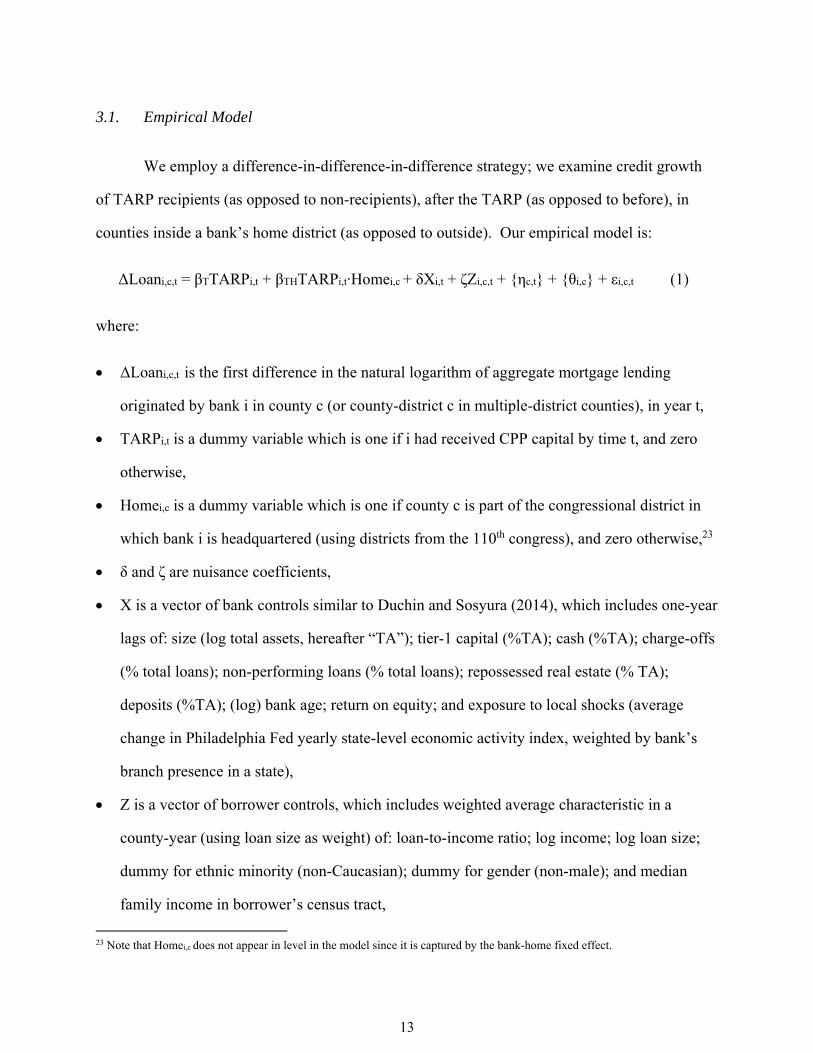
3.1. Empirical Model
We employ a difference-in-difference-in-difference strategy; we examine credit growth
of TARP recipients (as opposed to non-recipients), after the TARP (as opposed to before), in
counties inside a bank’s home district (as opposed to outside). Our empirical model is:
ΔLoani,c,t = βTTARPi,t + βTHTARPi,t∙Homei,c + δXi,t + ζZi,c,t + {ηc,t} + {θi,c} + εi,c,t (1)
where:
ΔLoani,c,t is the first difference in the natural logarithm of aggregate mortgage lending
originated by bank i in county c (or county-district c in multiple-district counties), in year t,
TARPi,t is a dummy variable which is one if i had received CPP capital by time t, and zero
otherwise,
Homei,c is a dummy variable which is one if county c is part of the congressional district in
which bank i is headquartered (using districts from the 110th congress), and zero otherwise,23
δ and ζ are nuisance coefficients,
X is a vector of bank controls similar to Duchin and Sosyura (2014), which includes one-year
lags of: size (log total assets, hereafter “TA”); tier-1 capital (%TA); cash (%TA); charge-offs
(% total loans); non-performing loans (% total loans); repossessed real estate (% TA);
deposits (%TA); (log) bank age; return on equity; and exposure to local shocks (average
change in Philadelphia Fed yearly state-level economic activity index, weighted by bank’s
branch presence in a state),
Z is a vector of borrower controls, which includes weighted average characteristic in a
county-year (using loan size as weight) of: loan-to-income ratio; log income; log loan size;
dummy for ethnic minority (non-Caucasian); dummy for gender (non-male); and median
family income in borrower’s census tract,
23 Note that Homei,c does not appear in level in the model since it is captured by the bank-home fixed effect.

14
{ηc,t} and {θi,c} are comprehensive sets of county-year and bank-home (district) fixed
effects, respectively, and
εi,c,t is a (hopefully) well-behaved residual, to represent all other determinants of loan growth.
The main coefficient of interest is βTH. The parameter captures the differential effect of
the TARP for mortgage growth in counties inside the bank’s home district. βT measures the
effect of TARP on mortgage growth in non-home district counties. We interpret robust
indications of a positive significant βTH to be evidence of a “home-district effect” associated with
political influences.
We begin by looking for such influences in all districts and thus for all representatives.
This is a conservative approach since some representatives are clearly more able and/or more
willing than others to cater to participants’ interest, for instance vis-à-vis the bank regulators
administering the TARP. Later on, we explore how the home-district effect varies with proxies
for the ability or inclination of a representative to help participants, like votes on key issues,
power in Congress or contributions received from the financial industry.
3.2. Estimation
We estimate (1) with four different techniques, clustering the standard errors by bank.
The main econometric challenge is that participation in the TARP could be correlated with post-
TARP characteristics of the participants’ home district, besides those linked to political effects.
For instance, a bank anticipating high credit demand in its home district could be more prone to
apply to the TARP, and to be accepted by the regulator. Alternatively, TARP banks could be
financially weaker, and may choose to cut lending first in distant areas while maintaining lending
in areas close to its headquarters where it has a comparative advantage in identifying profitable
15
investments (“home bias”).24 We address this challenge in three complementary ways: a) fixed
effects, b) a sample selection highlighting spatial discontinuities associated with political borders
and c) instrumental variables (we also pursue this issue further below in different ways).
We remove considerable unobserved heterogeneity via the two sets of fixed effects in (1).
The county-year fixed effects {ηc,t} control for credit demand and economic activity in a given
county-year.25 The bank-home fixed effects {θi,c} control for time-invariant heterogeneity
across banks and the way they behave in home and non-home-district counties, for instance
because of superior local knowledge.
3.3. Spatial Discontinuity
We further attenuate unobservable heterogeneity between home and non-home lenders
and counties by measuring ΔLoani,c,t using only loans inside a given county c (or district in a
multi-district county) that are originated in census tracts immediately adjacent to an intrastate
congressional district border. We can do so since our data reports the location of a borrower at
the level of the census tract, a small unit designed to contain a socio-economically homogeneous
population of about 7,000 individuals.
Of 77 Oklahoma counties, only 33 contain census tracts adjacent to an intrastate district
border (these counties are shaded in Figure 1); we drop the other 44 counties. Within the
remaining 33 counties, we then focus on census tracts next to district borders. The mean/median
OK county has 12.9/5 census tracts; rural counties have only few tracts, but urban counties have
24 Banks behave differently in markets closer to their headquarters since geographical proximity attenuates informational asymmetries (Petersen and Rajan, 2002), particularly so after downturns (Giannetti and Laeven, 2014; Chavaz, 2016). 25 Our home-district effect estimate could be biased upwards if TARP recipients receive more unsolicited applications in their home district. It is unclear whether or not unsolicited prospective borrowers might prefer to apply with a TARP recipient rather than with other lenders. Applicants might perceive TARP banks to have higher lending capacity due to lower funding costs, but applicants might also be wary of the stigma attached to TARP participation, perceiving it as a signal of underlying weakness (Berger and Roman, 2015). Either way, it seems implausible to us that this perception would prevail only a) inside the bank’s home district and not elsewhere, and b) for borrowers with higher unobservable quality. For robustness, we check for the possibility that TARP recipients received more unsolicited applications via county-year-TARP fixed effects.

16
many. Keeping only “frontier” census tracts allows us to increase the sharpness of
discontinuities (particularly in urban areas). This strategy is illustrated in the close-up map of the
Oklahoma County in Figure 2. The thick (black) lines again delineate districts, while thin (gray)
lines separate census tracts. Out of the 227 tracts in Oklahoma County, we only keep loans from
the 33 census tracts adjacent to district borders (shaded in Figure 2).
The goal of zooming onto “frontier” tracts is to make Homei,c irrelevant for non-political
reasons, like home bias. A bank headquartered in downtown Oklahoma City (in the 5th OK
district) might have superior information on future lending opportunities in the average
Oklahoma County tract, compared with “outsider” banks or counties. But it is less plausible that
this advantage also characterizes Oklahoma County tracts immediately next to the 5th district
border, especially by way of comparison with tracts immediately on the other side of the same
border. This restriction – combined with fixed effects and instrumental variables (see below) –
reduces the danger of our results being tainted by bank home-bias, and makes us comfortable
with assuming that unobserved home-district characteristics (such as expected local demand or
knowledge) cannot explain selection into TARP, and post-TARP lending growth. Since we
exclude areas contiguous to any district border which coincides with a state border, we also
attenuate differences due to bank regulation and supervision or the broader institutional
framework.
The drawback of the strategy is that it removes much of the data. Appendix A1 provides
further detail on this issue. In particular, we show that our approach does not seem to create
selection bias. We also show below that we obtain similar results using all census tracts,
suggesting that that our discontinuity approach adds safety to our identification strategy but is
not strictly necessary for our results.

17
3.4. Instrumental Variable Strategy
A third way to reduce concerns that participation in the TARP is correlated with post-
TARP district-level heterogeneity is to instrument for a bank’s TARP participation using pre-
determined bank characteristics. We follow Li (2013) and Duchin and Sosyura (2014) by
predicting TARP participation using connections with influential regulators and Congress
members. We first estimate a cross-sectional probit model of bank’s i participation in TARP:
TARPi = λConnectionsi + ψXi + ξi (2)
where
Connectionsi is a measure of connections for bank i. We use two measures of connections:
1. Fed director is one if an executive director of bank i served on the Federal Reserve’s
Board of Governors or the board of a regional Fed,
2. Subcommittee member is one for bank i if its home-district representative served on
the Financial Institutions and Consumer Credit Sub-Committee of the 111th Congress,
X are control variables, taken from equation (1), using 2008q3 values,
λ and ψ are coefficients to be estimated for instrument generation, and
ξ is a well-behaved residual. 26
After estimating (2), we retrieve the fitted values and interact them with a dummy
variable (unity post 2007, zero before) to create a time-varying instrument. That is, we form (
Connectionsi + Xi)∙It where It is one after 2007 and zero otherwise. We call this instrument
26 Fed director and Subcommittee member is 1 for 1% and 8.4% of 6,251 banks included in that regression, respectively.
18
TARP. To estimate βTH we follow the same procedure, but interact the IV additionally with our
home-district dummy variable, which we call TARP ∙ Home.27
Coefficient estimates from the first stages are presented in Table A2; it is immediately
obvious that ours are not weak instruments, satisfying the first requirement for a suitable
instrument. A second condition is that TARP ∙ Home affect ΔLoani,c,t only via its impact on
TARPi,t∙Homei,c rather than via factors excluded from model (1). In other words, TARP ∙ Home
should be uncorrelated with εi,c,t. Duchin and Sosyura (2014) show that committee memberships
are largely exogenous to bank lending behavior since they are allocated on the basis of federal
political outcomes and rotate regularly. It would take an even stronger assumption for the
exclusion restriction to be violated in our case given our difference-in-difference-in-difference
approach and extensive set of fixed effects: congressional sub-committee membership or Fed
directorship would have to be correlated with credit demand faced by TARP recipients only, only
in their home-district, and only after TARP, which seems implausible.
3.5. Propensity Score Matching
A final challenge is that participation in TARP could proxy for other bank characteristics
which could affect post-crisis home lending. For instance, financially weak banks could be more
likely to participate and to retreat home after the crisis, irrespective of TARP. Following again
Duchin and Sosyura (2014), we match samples consisting of a) all TARP recipients and b) their
closest non-recipient counterpart. To match recipients and non-recipients, we estimate a probit
model of TARP participation similar to (2), but without the political variables.28 We then match
27 One caveat: we lack information on bank applications to the TARP. Duchin and Sosyura (2012, 2014) have collected application information from banks’ annual reports or other communications. However, this information is only available for public banks, which are a minority in our sample. Duchin and Sosyura (2012) find that 80.2% of eligible banks applied, and that pre-existing connections do not correlate with application decision. 28 We also add a dummy for whether a bank is part of a Bank Holding Company [BHC] or not. We refer to BHCs informally as banks in the text below.
19
each recipient to a non-recipient using predicted participation probabilities, delivering propensity
score matching estimates of our key coefficients.
3.6. Data and Sample
We focus on the mortgage market, for two reasons. First, its intrinsic importance,
especially for the 2007-09 financial crisis which probably originated in the American housing
market. Second, the relevant dataset is of high quality and covers the majority of the American
market. All financial institutions are required to report their mortgage origination activity to the
FFIEC under the 1975 Home Mortgage Disclosure Act (HMDA) on a mandatory annual basis,
minimizing the selection bias present, for instance, in small business lending data.29 Crucially,
the dataset provides detailed borrower location information, a key requirement for our strategy.
We focus on data for the 2006-2010 period.30 From the raw dataset, we discard
applications received by non-commercial bank lenders (credit unions, thrifts, subprime
specialists, etc.), applications with incomplete location or income information, applications in
overseas territories, and applications for unusual products (multi-family dwellings and loans
guaranteed by the Veterans Administration or the Farm Service Agency). This leaves us with
44.8 million mortgage applications.
For each entry, HMDA reports whether the application was accepted, the identity of the
bank, loan-, borrower- and borrower-census-tract characteristics, including loan size, income,
race, and sex. The borrower location is reported at the level of the census tract. We use this
information to discard loans made in tracts not contiguous to an intrastate congressional district
29 The only HMDA reporting exemption is for banks under a size threshold (e.g. $36 mn in 2007) and banks without a branch in a Metropolitan Statistical Area (MSA). This means that the data covers the vast majority of mortgage lending, excepted in a few rural areas. Data can be downloaded from the FFIEC website (https://www.ffiec.gov/hmda/hmdaproducts.htm). The coverage is less comprehensive in the small and medium enterprise (SME) lending dataset stemming from the Community Reinvestment Act (CRA). We use this dataset as a robustness check below. 30 We use a relatively short window (2006-2010) for the baseline estimation to diminish the problem of banks exiting TARP. To check the importance of the window, we experiment with alternatives later on.
20
border (see above). We used Census Bureau maps for the 110th congress to map census tracts
into districts, and a relationship file from Brown University to identify contiguous tracts.31
Finally, we aggregate the data by bank-county-year (or bank-county-district year in multiple-
district counties). The final dataset spans 8,708 county-year and 5,272 bank-home combinations.
Since the majority of TARP recipients were bank-holding companies (BHCs) rather than
banks, we aggregate lending data to the BHC level, and refer to “banks” for convenience in what
follows.32 We typically do not include data for the nineteen biggest US banks, those which
participated in the Fed’s 2009 SCAP stress test; since they were forced to participate in the
TARP, there is no way to separate the effect of TARP from the effect of being a systemically
important bank.33 We also drop foreign-owned banks ineligible for the TARP, and banks for
which we cannot find the end-2007 headquarter in Call Reports.
We add data on TARP recipients taken from the US Treasury’s website and merge it with
HMDA data using the recipient’s name.34,35 The data indicates the size and timing of capital
injections, as well as the dates of the initiation and completion of repayment, if applicable. 672
distinct firms (mostly banks) participated in TARP; 204 entered the program in 2008, and
another 468 in 2009. We observe 444 of the 672 participants in our full bank-county-year
mortgage lending.36 The FDIC’s Call Reports database provides us with bank-year controls and
the unique regulatory identifier of a bank and its parent BHC. We aggregate all these controls to
31 See http://www.s4.brown.edu/us2010/Researcher/Pooling.htm. A limited number of tracts can be attributed to more than one district; we drop loans granted in these tracts. 32 We map the bank identifier provided in HMDA into a BHC identifier using the Regulatory High Holder identifier provided in bank Call Reports. For banks unaffiliated to a BHC, we aggregate data at the bank level. 33 Duchin and Sosyura (2014). We check for the importance of this exclusion below by including these banks in a sensitivity check. 34 See treasury.gov/initiatives/financial-stability/reports/Pages/default.aspx. 35 We thank Anya Kleymenova for kindly sharing her merging file. 36 We do not observe the remaining 228 participants for a variety of reasons: some participants do not do mortgage lending at all (e.g. American Express); others are too small or too little present in urban areas to be covered in HMDA; some participants are missing data (e.g., 2007 headquarter location); some are removed because of the filters we apply (e.g. dropping the top-19 banks like Bank of America). 383 of these 444 participants remain in the final benchmark sample once we filter out loans in non-contiguous tracts.
21
the BHC-year level. The BHC-level Call Reports provide us with the BHC’s headquarters
location.37 We use the end-2007 bank headquarters location, to rule out strategic relocation after
the crisis. We again map the headquarter location into districts using Census Bureau maps.38
We merge HMDA and Call Reports data using the regulatory identifier provided by HMDA.
Finally, we find data from the House of Congress website on congressional
representatives, membership in key committees, and voting behavior for TARP-related roll calls.
Data from service on Federal Reserve Bank boards are from Li (2013).39
3.7. Summary Statistics and Parallel Trends Assumption
Appendix A2 provides descriptive statistics and discusses the timing of the shock as well
as the validity of the parallel trends assumptions. Average home and non-home lending trends
are roughly comparable for participants and other banks before TARP. After TARP, participants
cut non-home lending drastically whereas home lending remains comparable for the two groups.
This effect is reversed in 2010, when most participants have exited the program. While
necessarily informal, we find this result interesting; it proves to be consistent with our more
rigorous statistical work. We now turn to the latter to confirm the “home-district” effect using
our regression framework.
37 Bank- and BHC-level Call Reports can be downloaded from the Federal Reserve Bank of Chicago website (https://www.chicagofed.org/banking/financial-institution-reports/commercial-bank-data and https://www.chicagofed.org/banking/financial-institution-reports/bhc-data, respectively). 38 In single-district counties, we map bank headquarters into districts using the Census Bureau relationship file. For banks with headquarters located in counties with multiple districts, we either use the headquarters’ zip code and combine it with a ZCTA-District and ZIP-ZCTA relationship file from the Census Bureau, or headquarters’ geographical coordinates (from Summary of Deposits) mapped into districts using our own geo-coding routine. We drop the few banks whose headquarters can be attributed to multiple districts. 39 We thank Lei Li for kindly sharing the data for his instrument.
22
4. Main Results
4.1. Benchmark Estimates
Our benchmark results are presented in Table 1, which tabulates estimates from OLS
(column 1), both sets of instrumental variables (IV, in columns 2-3), and propensity score
matching (PSM, in column 4). We tabulate the {β} coefficients of interest: the effect of TARP
on mortgage-loan growth outside the home-district, and whether this effect differs significantly
between areas inside and outside the home-district (other estimates are available online).
The effect of the TARP on mortgage lending outside the home-district, tabulated in the
second row, is mixed. In particular, the coefficient tabulated on the bottom row, βT, is
statistically insignificant and small for OLS and PSM estimators, negative and significant for
both IV estimators. In other words, banks that received TARP funds either maintained or cut
lending for areas outside their home-district. Still, our main interest is in the top row, which
tabulates estimates of the home-district effect, βTH, on loan origination.40 In contrast with the
small or negative effect of the TARP outside the home-district, the parameter for TARP x Home
indicates that the effect of TARP inside the home district is highly significant, both statistically
and economically. Our OLS estimates indicate that mortgage lending grows (exp(.22)-1≈) 25%
more in home districts; the PSM estimate is comparable. IV estimates suggest an even larger
effect, indicating that the TARP leads to around (exp(.47)-1≈) 60% more lending in the home
district. The fact that IV estimates are larger than the OLS/PSM estimates is consistent with IV
measuring the local treatment effect of receiving TARP funds as soon as the possibility opens up
(results in section 5 show that early recipients are more prone to political influences), and partly
40 The coefficient measures whether more loans are originated within the home-district of the bank, ceteris paribus; because some of these loans will be securitized, agents outside the home district will eventually hold some of the mortgages. It is unclear whether this would be of relevance to the relevant politicians.
23
thanks to political connections. All four (OLS, IV, and PSM) estimates are statistically different
from zero at the 1% level.
The average home-district lending growth of TARP participants can be gauged by adding
the parameter estimates for TARP and TARP x Home. This sum ranges from 0.06 (second IV
regression) to 0.17 (OLS regression). But the t-test p-values reported at the bottom of Table 1
show that these sums are different from zero in the OLS regression only. In other words, TARP
participants do not necessarily boost lending inside their home district; instead, they seem to
shield home-district counties from the lending cuts they impose elsewhere. This interpretation
coincides with the visual reading of lending trends in Figure A1 (see section 3.7).
4.2. Sensitivity Analysis
Table 2 reports sensitivity analysis for the key coefficient, βTH, the estimate of the home-
district effect. We consider seventeen perturbations to our benchmark methodology, and tabulate
OLS, IV, and PSM estimates in Panel A of Table 2; our default estimates from Table 1 are
recorded on top to facilitate comparison.
First, we consider slightly different regressands. We successively and separately
eliminate: loans purchased by Government-Sponsored Enterprises, loans guaranteed by the FHA,
and refinance loans. The home-district effect remains positive and statistically significant
throughout these perturbations. We then try shorter (2006-2009) and longer (2005-2012) sample
periods. We obtain similar results, though they are economically smaller for the larger window.
Our next checks involve exploring alternative sets of banks and geographies. First, we
include all loans, instead of only those made in tracts contiguous to district borders; this
marginally reduces the economic magnitude of our estimates. We then successively: a) add back
the largest (nineteen) American banks (those who participated in the 2009 stress test), b) drop the
24
top-30 banks (the 2014 CCAR participants) and c) drop all banks headquartered in New York
City. Our results are economically and statistically somewhat smaller, but still significantly
different from zero at the 5% level; our results are not driven by “mega-banks”.
We then check the importance of controls. To account for changes in the observable
quality of applicants across different banks and counties, we replace bank-county-year borrower
controls by comparable bank-county-year applicant controls. This does not materially change
results. Dropping all the bank controls also has little effect on our results. We then explore an
alternative definition of Home, which is unity not only in a BHC’s home district, but also in any
of its subsidiaries’ home districts.41 The resulting home-district effect is essentially unchanged.
Another issue to consider is the importance of outliers; we pursue this in two different
ways. First, we winsorize all variables at the 1% level. Alternatively, we drop outliers, defined
as observations with residuals lying more than two standard deviations from the mean. Our
results remain statistically solid through these checks, but the economic magnitude falls by
around a quarter in the second perturbation. This suggests that our headline economic estimates
are somewhat inflated by observations with extreme lending growth. We then experiment with
standard errors, using state-level clustering. We obtain smaller standard errors, confirming that
bank-clustering is more conservative. Finally, we replace bank-home fixed effects with bank-
county fixed effects; this is of little consequence.42 To summarize our sensitivity analysis: the
home-district effect does not depend on minor features of our sample and model specification.
4.3. Alternative explanations
41 Our baseline set-up assumes that BHCs (or banks in the case of independent banks) are connected to the representative for the district in which the BHC is headquartered; this alternative definition accounts for the possibility that political connections also exist between BHCs and representatives of the districts in which subsidiaries are headquartered. We make this assumption to conform to the facts that a) TARP funds were granted at the BHC level, and b) connections between a BHC and its home-district representative predict participation in the TARP (Duchin and Sosyura, 2012).
42 The same is true of using bank-district fixed effects, as we did in earlier versions of the paper.
25
Our next set of tests addresses four alternative explanations for the home-district effect:
gerrymandering, credit demand, home bias, and other differences between banks and their
borrowers. Our results are reported in Panel B of Table 2. We first drop all loans granted in the
40 most gerrymandered districts, as identified by Mackenzie (2009) based on their
geographically abnormal shapes. The results change little; gerrymandered districts are not the
source of our finding. 43
Second, we replace county-year with TARP-county-year fixed effects, again finding
comparable results. This suggests that the home-district effect cannot be explained by changes
in average credit demand faced by TARP recipients in their home-district (the application-level
evidence below demonstrates this more directly).
Third, we control for several possible manifestations of home bias. We start by adding a
control Crisis x Home, where Crisis is unity after 2008, and zero otherwise. This allows us to
capture any general retrenchment towards the home district, for instance if banks seek to
strengthen their connection with the home-district representative in a context of impending
regulatory overhaul, irrespective of participation in TARP. The OLS/PSM estimates are
unaffected, and the IV estimates are higher. This suggests that the home-district effect operates
over and above any crisis-induced extra home bias effect.44
Our results could also reflect a home bias specific to TARP participants. TARP banks
might be weaker and thus more prone to cut lending. In turn, weak banks might want to cut
lending first in those markets in which they do not have superior information, like distant
43 Gerrymandering could bias our results upwards if it increases the sharpness of the discontinuity between politically heterogeneous but economically similar areas. Alternatively, gerrymandering could bias our results downwards if abnormal district shapes make it unlikely that a bank only maintains relationships with the representative of its home district. We have also checked that the home-district effect is not statistically different for the most gerrymandered districts. 44 If we substitute 2007 for 2008, the IV estimates remain essentially unchanged, but the OLS and PSM estimates fall to 0.16 (0.09) and 0.16 (0.07) respectively.
26
counties (Landier et al., 2007; Giannetti and Laeven, 2012) or quantitatively less important
counties. This could bias our results if these “core” counties also lie within banks’ home district.
We explore this TARP-specific home-bias in three ways. First, we add a control “Close
to Headquarter” which is one if the distance between a given county and the county where the
bank is headquartered is smaller or equal to the 5th percentile for a given bank-year, and zero
otherwise.45 We then interact this control with TARP. The economic size of the home-district
effect diminishes somewhat, but our key conclusion is unchanged. Second, we add a dummy
“Home County” – unity in the county where a bank is headquartered, and 0 elsewhere. Unlike
congressional districts, counties do not delineate areas with obvious differential exposure to
federal politics. Thus, TARP recipients should not face any political incentive to increase
lending in their home county, other than because of its overlap with the home district. But if our
results are driven by distance rather than by political factors, the home-county border could
matter. In that case, adding this control should reduce the size of the home-district effect. The
results suggest otherwise; the economic magnitude of TARP x Home changes little.
Banks might be headquartered in richer, urban areas; markets close to headquarters might
also account for a bigger share of the bank’s business. So yet another form of home bias is that
weak banks could cut lending more in poorer, rural or smaller markets, and less in richer, urban
or bigger markets they know better. We thus first control for “Rich County” (and its interaction
with TARP) – unity if county borrower income is above the bank-year median, and zero
otherwise. We then control for “County Importance” – the percentage of a bank’s total lending
in a given county before TARP (2006-2007), and interact it with TARP. Adding these two
controls separately does not change our results.46 We then run the baseline regression separately
45 Results are unchanged when we use the 10th, 15th, 20th and 25th percentile instead. 46 We find comparable (unreported) results when alternatively controlling for the market share of a bank in a given county before TARP (2006-2007), and its interaction with TARP. This indicates that our main result is not explained by a “flight” of TARP banks towards markets where they have a dominant position.
27
for a) rural counties (counties in a single district) and b) urban counties (counties spanning
multiple districts). The home-district effect remains significant in both samples, with only minor
differences in statistical and economic significance.
Together, these tests indicate that the home-district effect is not explained by home-
district credit demand, or by a reluctance to cut lending in closer, richer or bigger markets.
One final challenge is that TARP and non-TARP banks could differ along finer
dimensions than their overall propensity to participate (as controlled for in our baseline PSM),
for instance their capitalization; home and non-home districts could also differ along other
dimensions than political ones, for instance their affluence. Given our difference-in-difference-
in-difference approach, both these challenges should hold at the same time to bias our results. In
Appendix A3, we confirm that our main result is similar when matching participants and non-
participants based on every individual bank and borrower characteristics in our sample, and
when adding a range of additional TARP x County characteristic controls.
4.4. Placebo Test
We also add a placebo test, in which we falsify the timing of the shock. We assume that
the TARP recipients receive an equity injection three years before the actual date; we then
estimate the baseline regression for the 2003-2007 period. The home-district coefficient is
economically and statistically insignificant for all estimators; this suggests that our main result is
not driven by different pre-shock trends across recipients and non-recipients.47
4.5. Application-level Evidence
47 We reached a qualitatively similar conclusion in the 2016 NBER working paper version of this study, but we had found different coefficients as a result of inadvertently leaving the top-19 banks inside the sample.
28
As a final check on our identification strategy, we exploit our mortgage data at the most
disaggregated level, that of the individual mortgage application. We estimate the model:
Acceptedi,a,c,t = βTTARPi,t + βTHTARPi,t∙Homei,c + δXi,t + ζZi,a,c,t + {ηc,t} + {θi,c} + εi,a,c,t (3)
where:
Acceptedi,a,c,t is 1 if bank i accepts application a in census tract c and year t, and 0 otherwise,
Bank controls, borrower controls and the bank-home fixed effect θi,c are similar to the
baseline model,48 and
The location-time fixed effects are discussed below.
The application-level analysis gives a distorted picture of the average home-district
effect, since it a) overweighs large banks and areas and b) only captures changes in acceptance
rates, not lending volume. If a TARP recipient aggressively solicited applications (in line with
anecdotal evidence in section 2) or used its funding advantage to outbid its competitors without
increasing risk-taking, this model would not capture it.
However, this approach has two benefits. First, we can estimate the differential effect of
the TARP a) within a given neighborhood and year (via census tract-year fixed effects) and b)
across a pair of neighborhoods located on either side of an intrastate district border (via census
tract pair-year fixed effects). Second, since it models a mortgage supply decision conditional on
a given mortgage demand, this approach removes unobservable individual demand-side effects.
Together, these can help us gauge the robustness of our identification strategy.
We use two alternative sets of fixed effects. First, we replace the county-year fixed
effects (used in the baseline model) with census tract-year fixed effects (henceforth, “within-tract
48 A minor difference is that borrower controls appear at the borrower level rather than as a bank-county-year average as in the baseline regression. Specifically, Z includes: loan-to-income, log loan size, log income, and binary variables for borrowers that are black, Latino and non-male. We do not include the tract-level borrower controls used in the baseline regression since they are picked up by the tract-year fixed effects.
29
model”). This controls for credit demand and unobservable borrower quality in a neighborhood,
period by period. Combined with the alternative dependent variable, this approach is the most
conservative way to control for demand factors feasible using HMDA data.
Second, we retain tract-year fixed effects, but replace the bank-home fixed effects (of the
baseline set-up) with bank-census pair fixed effects (henceforth, “across census pairs model”).
This allows us to control for unobserved heterogeneity in the way a given bank behaves on
average within a pair of two census tracts located on either side of an intrastate district border.49
Given the extensive potential number of observations and fixed effects, we drop loans
which play no role in our baseline results according to our robustness checks (see Table 2),
namely loan purchased by GSEs, loans guaranteed by the FHA and refinance loans.50 We do not
report IV estimates since they often fail to converge, given the large number of fixed effects.51
The results in Table 3 indicate a positive and strongly significant coefficient for TARP x
Home. This is true for both OLS and PSM estimates, and for both models (within census and
across census pairs). For instance, the OLS estimate of the within-tract model (column 1)
indicates that, controlling for his/her characteristics, an applicant’s chance to be accepted is 4%
higher if he/she applies with a TARP recipient, and his/her house is located in the bank’s home
district. We find comparable estimates in the other three columns. In contrast, the coefficient
for TARP is always negative but statistically insignificant, indicating that borrowers are treated
insignificantly different outside a TARP bank’s home district. We conclude that at least a
49 Since they vary in size and shape, a majority of census tract can be paired with multiple census tracts on the other side of the border (2.3 on average). Thus, a given observation must be included several times in some cases for this model to be identified; specifically, applications must appear once for each possible pair they can be attributed to. For instance, an application from a tract that can be matched to three different tracts on the other side of the border must be included three times in the dataset. 50 This also allows us to focus on applications for which banks have the greatest margin of discretion. In particular, GSE loans are typically underwritten automatically using the GSEs’ own software and standardized data, leaving little discretion for alternative considerations (such as political ones) to be factored into screening decisions. Refinancing loans also leave less discretion to banks, since the ability to observe the applicant’s payment history reduces contracting frictions (Gilje et al., 2016). 51 Since non-linear models are biased in the presence of high-dimensional fixed effects, we estimate the application-level model via OLS despite the binary dependent variable (Puri et al., 2011; Duchin and Sosyura, 2014).

30
portion of the home-district effect can be ascribed to TARP recipients’ willingness to accept
applications from their home district disproportionately.
4.6. External Validity: Small Business Lending
Our focus on the mortgage market is partly motivated by data considerations. The
HMDA is the only comprehensive database containing precise information on the geographic
location of borrowers. In principle however, there is no reason why the home-district effect
should not hold for other markets, such as those for commercial and industrial lending. Banks
are the single most important source of credit for small firms, and recipients’ small business
lending was an important focal point of TARP surveillance bodies such as the Congressional
Oversight Panel, as well as media discussions around credit supply after the crisis and TARP.52
Such concerns may well have opened the door to political influences similar to those at work in
the case of mortgage lending.
Accordingly, we investigate the home-district effect in the small business lending market.
We use a panel of small business loans for the 2006-2010 period collected under the auspices of
the Community Reinvestment Act (CRA). The CRA dataset has two main disadvantages
compared with the HMDA database. First, although a majority of American banks file CRA
reports, participation is voluntary. Second, the publicly-accessible version of CRA aggregates
lending to the bank-county-year level, where HMDA reports application-level data. This has
two implications for our methodology. First, one cannot explicitly control for borrower
characteristics (the vector Z), at least beyond those captured by a county-year fixed effect.
Second, we cannot zoom onto loans within a given county granted in census tracts contiguous to
district borders. Instead, we focus on counties which are contiguous to congressional district
borders, within the same state. Note that since urban counties often have multiple districts, this 52 See e.g. Congressional Oversight Panel (2010), “The Small Business Credit Crunch and the Impact of the TARP”. Available for download from www.gpo.gov.
31
implies that the sample in this regression is biased towards rural areas. With those exceptions,
our empirical model is the same as that of our baseline model (1).
Table 4 reports OLS, IV, and PSM results for small business lending analogous to those
of Table 1. We find similar results to the mortgage regressions. The coefficient for the home-
district effect ranges from 0.21 (PSM) to 0.48 (IV). As expected from the poorer data quality
and identification, the precision of the effect is lower than with mortgages. The OLS estimate is
significantly different from zero only at the 10% level, though the others are significant at the
5% level. The TARP coefficient is never significantly different from zero in any of the
equations. In other words, the TARP has no significantly discernable effect on small business
lending except inside the recipients’ home-representative congressional district.
These results provide an independent check for our mortgage results; the fact that we find
qualitatively and quantitatively similar results with a different dataset suggests that the home-
district effect is robust to idiosyncrasies associated with the mortgage market or HMDA data.
5. Variation across time, banks, and politicians, and aggregate and electoral effects
We have established the existence of a “home-district” effect; recipients of public capital
injections have higher lending growth inside their home-representative’s congressional district
than outside. That is, the nature of mortgage and small business lending by TARP recipients
appears to have been influenced by political considerations. In this section, we provide
additional evidence to supplement and strengthen our interpretation.
The political economy literature and anecdotal evidence surveyed in section 2 suggest
two possible reasons for our findings. First, recipients might want to (or be compelled to)
reciprocate a “favor” provided by their home representative. This can include direct help in
entering or exiting the program, as well as other congressional actions before and after the
32
inception of funds which are particularly beneficial to a participant.53 Second, recipients might
seek to preempt political interference. Access to public funds attracts political and media
scrutiny on banks. Evidence in section 2 suggests that a) politicians could use platforms like
Congressional hearings to pressure participants, and b) participants could use evidence of
lending in key areas to counter (or pre-empt) criticisms on their lending behavior.
These mechanisms are neither observable, nor mutually exclusive; we thus do not attempt
to disentangle them.54 Instead, we explore predictions consistent with either channel.
Specifically, our key interest is to test whether the home-district effect is stronger in periods,
banks and politicians where the scope or motive for political intervention and/or the incentive of
the bank to be responsive to political influences (or the threat thereof) is higher. Panel C in
Table A3 reports summary statistics for the proxies used to test these predictions.
5.1. Timing
We start by investigating whether the timing of the home-district effect coincides with
periods during which politicians have the greatest scope to intervene, and banks are most liable
or vulnerable to interference. We explore two proxies. First, political influences should be
stronger around the capital injection time. We thus create three separate dummies TARPt,
TARPt+1 and TARPt+2 , which are, respectively, unity during the year the bank enters the TARP,
one year after, and two years after, and zero otherwise. We then interact these dummies with
Home. We find that TARPt x Home and TARPt+1 x Home are significant at 1% confidence level
and of comparable economic size. (The sum of these two coefficients is reported in column 1 of
53 For instance, the Washington Post reports that “Rep. Barney Frank (D-Mass.) … wrote language into the bailout bill that effectively directed the Treasury to give special consideration to [Massachusetts bank] OneUnited, and he followed up with a call to Treasury. The bank got $12 million.” http://www.washingtonpost.com/wp-dyn/content/article/2009/07/01/ AR2009070103694.html 54 It would be conceptually useful to distinguish between them since the second mechanism suggests that political influences can bind even without explicit politician interference. But given their substantial observational overlap, we do not believe to have sufficiently precise data to cleanly separate these two arguments in the data.
33
Table 5). But TARPt+2 is insignificant. Consistent with intuition, the home-district effect is thus
concentrated around the injection date.
Second, political influences should be stronger as long as the bank holds TARP funds,
and its home representative at the start of the program is in office. We thus create a dummy
“Exit” (and its interaction with Home) – unity if a bank has repaid TARP funds, or its 2008
home representative is no longer in office after the November 2008 elections, and zero
otherwise. The results tabulated in column 2 of Table 5 show that the home-district effect
reverses once the recipient’s relationship ceases to either the TARP or the bank’s original home
representative. TARP x Home x Exit is negative and significant; this suggests that TARP
recipients decrease home-district credit growth when this relationship ceases.55
5.2. Bank characteristics
We have established that the timing of the home-district effect coincides with periods of
greatest possibility of political influence. We now explore whether the effect is also stronger for
those banks with more scope for such influence, or a bigger incentive to respond to it.
We consider two proxies. First, anecdotal evidence suggests that applicant banks helped
by politicians access TARP during the first round of the distribution of CCP funds. The Wall
Street Journal first reports about political interference on 22 January 2009; five days later,
Treasury Secretary Geithner announces rules to prevent lobbying on behalf of applicants. This
should restrict the scope for political interference during the two next application rounds.56
55 In contrast, TARP x Exit is positive and significant; recipients increase lending growth out of their home district once they are no longer liable. This reversal is only partial. The decrease in home-district credit growth when the relationship to TARP or the initial representative terminates is -0.12 (≈0.40+0.28), against +0.28 when the relationship is still going on. 56 http://www.nytimes.com/2009/01/28/business/economy/28lobby.html. The first application window opened from October 14 to November 14, 2008. In January 14, application was opened again for a month to qualifying S-corporations. Finally, a third application window was opened on 13 May, 2009 for banks with total assets below 500 Million (Millon Cornett et al., 2013).
34
To explore application timing while avoiding endogeneity issues, we exploit two aspects
of bank organizational structure. Specifically, the first application round was opened only to
public banks. One reason is that many privately held banks are organized as “Corporation S”, a
type of firms which can only have one class of shareholders. The Treasury was thus initially
unable to purchase preferred stock in these banks as foreseen by the terms of the TARP. We
thus construct a dummy “Eligible for 1st round” – unity if a bank is a) publicly traded and b) not
a Corporation S, and zero otherwise. The results tabulated in column 3 of Table 5 show that the
interaction of Eligible and TARP x Home is positive and significant. In other words, the home-
district effect is higher for potential first-round recipients, in line with our intuition.
Our second proxy explores the role of bank risk. The TARP was not intended as a
bailout of unhealthy banks. Bayazitova and Shivdasani (2012) and Duchin and Sosyura (2012)
confirm that riskier applicants were less likely to be accepted. Specifically, the finding common
to both studies is that banks with greater funding risk are less likely to be accepted. We thus
create a proxy “Deposit-to-asset ratio” measured as the share of bank total assets in the form of
deposits in 2008q3. The results in column 4 show that the interaction of Deposit-to-asset ratio
and TARP x Home is negative and significant. This suggests that participants that were less
likely to be accepted are more subject or responsive to political influences or the threat thereof.57
5.3. Politician characteristics
We have established that the home-district effect coincides with the periods and banks
most susceptible to political interference. We now explore whether the effect also changes with
proxies for politicians willingness and ability to help banks as part of TARP, or more generally.
57 We find qualitatively similar results when using the share of undrawn lending commitments to total assets as alternative measure of liquidity risk (Millon Cornett et al., 2013). Bayazitova and Shivdasani (2012) and Duchin and Sosyura (2012) also investigate the role of solvency risk as measured by bank capitalisation, but do not find any significant effect on acceptation. In unreported results, we similarly find that pre-TARP capitalisation does not change the home-district effect.
35
We consider three proxies of the willingness of politicians to help banks. We begin by
investigating the role of TARP votes in Congress. Most representatives featured in anecdotal
evidence in section 2 were TARP supporters. We assume that intervening in favor of applicants
or pressurizing participants to lend is less costly for TARP supporters. More broadly, the TARP
vote provides an indicator of revealed preferences to help banks, as it was largely determined by
a representative’s proximity to the financial industry (Mian et al., 2010).58 Finally, the TARP
vote was tight; individual politicians seeking to help firms can thus make a difference (Cohen
and Malloy, 2014).59
Accordingly, we re-estimate baseline model (1), additionally controlling for the dummy
“TARP supporter” – one for banks whose home representative supported the TARP, and zero
otherwise. Our main coefficient of interest is the term TARP x Home x TARP supporter; this
captures how the home-district effect changes with the vote. Column 5 in Table 5 shows that the
home-district effect increases significantly with a ‘yes’ vote. Specifically, the home-district
effect is 0.34 (≈0.38-0.04) for ‘yes’-vote banks, against -0.04 for ‘no’-vote banks. In other
words, political considerations seem to only influence recipients’ lending if its representative’s
vote aligns with bank special interests.60
As a second proxy for politicians’ willingness to help banks, we consider contributions
received from the financial industry. Politicians receiving more contributions are more prone to
cater to banks’ special interests in Congress, and thus represent a potentially more valuable
connection in a context of crisis and regulatory overhaul. Accordingly, we use Mian et al.
58 In contrast, the TARP vote does not correlate with mortgage defaults in the representative’s district. 59 The Emergency Economic Stabilization Act (EESA), the legislation that created the TARP, was voted down 205-228 on Sept 29, 2008 before being voted through 263-171 on Oct 3, 2008. We focus on the latter vote in the tests below. 60 We also tested whether the home-district effect is stronger if the representative had voted for the 2008 American Housing Rescue and Foreclosure Prevention Act (AHRFPA), a federal program supporting mortgage renegotiations and GSEs. Unlike the EESA, the AHRFPA targeted constituent interests (those of underwater mortgagors), rather than those of the financial industry (Mian et al., 2010). In unreported results, we found that TARP x Home x AHRFPA supporter is statistically insignificant. The home-district effect thus does not seem to vary with votes on objects benefiting constituent interests rather than those of banks.

36
(2010)’s database to construct a variable “Financial contributions” which corresponds to the
(log) amount received by a bank’s representative up to November 2008 from a Political Action
Committee affiliated to the financial industry, as measured by the Center for Responsive
Politics.61 The interaction of Financial contributions with TARP x Home captures whether the
home-district effect increases with the home-representative’s connection to the financial
industry. Our result is tabulated in column 6 of Table 5. Consistent with our intuition, we find
that the triple interaction term of interest is positive and significant at the 5% confidence level.62
Third, a politician’s willingness to help a bank should also increase with the importance
of the bank for its district. Cohen et al. (2013) show that politicians are more prone to cater to a
firm’s interests if it can have a sizable impact on economic activity in his/her district. We thus
create a variable “District market share” which is the bank’s share of mortgage origination in its
home district before TARP (2006-2007). The results in column 7 of Table 5 confirm our prior:
the home-district effect increases significantly with the home-district market share. Specifically,
the estimate for the TARP x Home x District market share interaction (2.03) suggests that the
home-district effect is 0.23 for a bank with an average market share (9%) and increases to 0.52
when the market share increases by one standard deviation (14%).
Finally, we explore the ability of politicians to help or pressure firms. To do so, we
consider membership in key committees (Duchin and Sosyura, 2012; Agarwal et al., 2016; Akey
et al., 2016). Powerful politicians have more sway in Congress and, presumably, over
government. They were thus in a good position to help applicants at the start of the program, and
to influence key legislation affecting the terms of TARP after it had been launched. Table A6
shows that one committee of the 110th Congress worked on bills related to TARP, and another
61 We remove banks whose representative was not re-elected in 2008 from the sample for this regression since we do not have contributions data for newly elected representatives. We do the same for the TARP supporter test for a similar reason. 62 We find comparable economic and statistical significance when running this regression in a subsample of banks whose representative supported the TARP. Political contributions thus matter independently of their effect on the TARP vote.
37
three in the 111th Congress. We thus create a dummy “Powerful politician” which is one for a
bank whose home representative sat on one of these committees during the corresponding period.
Column 8 in Table 5 shows that the interaction of this dummy with TARP x Home is positive
and significant. Specifically, the home-district effect is 0.39 (≈0.31+0.08) for participants with a
powerful home representative, against 0.09 for other participants. Political considerations thus
seem substantially stronger for banks connected to a powerful politician.63
Together, these results reinforce the interpretation that political influences (or the threat
thereof) influence lending decisions in periods, banks and politicians where the scope or motive
for political interference and the incentive on the part of the bank to respond to them or pre-empt
them is higher. The evidence presented in this section is supplemental, not definitive. Still, it is
consistent with the notion of a reciprocal political channel that steers mortgage growth after the
TARP towards areas within the district borders of the bank’s congressional representative.
5.4. Aggregate and electoral effects
Thus far, our tests use only parts of the available data, split across counties and banks for
cleaner identification; this raises a question of whether the home-district effect matters in the
aggregate for politicians, their constituents and TARP participants, as our interpretation
implicitly suggests. In the appendix section A4, we provide three results supportive of this
notion. First, districts in which locally headquartered TARP participants have a 10% higher
market share experience 4.2% higher growth in total lending after TARP. Second, improved
lending conditions go along with improved electoral prospects for incumbents during the 2010
House of Representatives elections, with a magnitude close to the effect of higher federal
spending in a district for incumbent vote percentage (Levitt and Snyder, 1997). Finally, TARP
63 Politicians’ attempt to join key 111th Congress committees could be correlated with banks in their home district participating in TARP. To rule out this possibility, we re-estimated this regression assuming that Powerful representative is 1 only for a representative who already sits in a key committee in the 110th Congress. We find similar results (available upon request).
38
participants with a higher share of home-district mortgages in their overall loan portfolio
experience more non-performing loans after TARP. Aggregating data necessarily reduces
statistical power and identification precision, so we interpret magnitudes with caution. But at
face value, these results support the hypothesis that the home-district effect matters in aggregate
for politicians, constituents, and banks.
6. Conclusion
Government-funded programs are necessarily shaped and approved by parliaments, and
allocated discretionarily by public bodies. This leaves scope to politicians to influence the
availability and terms of funds to firms they are connected to. In this paper, we have examined
the consequences of a large political intervention for the allocation of corporate investment
across political constituencies. We have documented the existence of a “home-district effect”;
banks that received capital from the Troubled Asset Relief Program (TARP) lent 23%-60% more
in their home-representative’s congressional district than elsewhere. We have also provided
evidence that suggests that this higher lending improved the electoral prospects of incumbents
while also reducing the quality of banks’ mortgage portfolios.
The key contribution of these findings is to document evidence that investment decisions
by beneficiaries of government funds are subject to political influences. Our findings also show
that political forces matter despite the maturity of the American political and financial systems
and the absence of formal channels for politicians to influence bank lending decisions.64 Of
course, we do not know whether our result is general, or an idiosyncratic result of an exceptional
64 Members of key Congress committees obtain bank loans at preferential terms (Tahoun and Vasvari, 2016). Collusion between politicians and local banks have contributed to the long-standing regional fragmentation of the American banking system (Kroszner and Strahan, 1999), and to limits on access to credit in early 20th Century America (Rajan and Ramcharan, 2011).
39
financial intervention during a financial crisis. Other government funding programs like
procurement contracts may constitute insightful laboratories for further research.
From a policy perspective, our results bear on discussions around newly created cross-
border bank funding and resolution arrangements such as the European Stability Mechanism
(ESM). Our results suggest that conflicting local interests may steer the impact of bailout
programs, even in areas as politically and financially integrated as the United States. This
suggests that international mechanisms may find it even more difficult to mute conflicting
national interests over bailouts and the associated impact on credit supply.
Our study also adds to the debate concerning the causes of the credit fragmentation that
followed the global financial crisis (e.g., Giannetti and Laeven, 2012). We do not explicitly
search for evidence of aggregate post-crisis financial fragmentation in the United States.
Nevertheless, our results are consistent with the hypothesis that financial fragmentation can
result from “financial protectionism,” that is, a distortion of credit flows towards the local
economy after large government intervention in the financial sector (Rose and Wieladek, 2014).
40
References
Agarwal, Sumit, Gene Amromin, Itzhak Ben-David, and Serdar Dinç (2016) “The politics of foreclosures” Unpublished. Agarwal, Sumit, David Lucca, Amit Seru, and Francesco Trebbi (2014) “Inconsistent regulators: Evidence from banking” Quarterly Journal of Economics 129 (2), 889-938. Akey, Pat, Heimer, Rawley Z., and Stefan Lewellen (2016) “Politicizing consumer credit” Unpublished. Akin, Ozlem, Nicholas S. Coleman, Christian Fons-Rosen, and José-Luis Peydró (2016). “Political connections: Evidence from insider trading around TARP” Unpublished. Amore, Mario Daniele, and Morten Bennedsen (2013) “The value of local political connections in a low-corruption environment” Journal of Financial Economics 110 (2), 387-402. Antoniades, Alexis, and Charles W. Calomiris (2016). “Mortgage market credit conditions and US presidential elections” Unpublished. Bayazitova, Dinara, and Anil Shivdasani (2012) “Assessing TARP” Review of Financial Studies 25 (2), 377-407. Behn, Markus, Rainer Haselmann, Thomas Kick, and Vikrant Vig (2015) “The political economy of bank bailouts” IMFS Working Paper 86. Berger, Allen N., and Raluca A. Roman (2015) “Did TARP banks get competitive advantages?” Journal of Financial and Quantitative Analysis 50 (06), 1199-1236. Bertrand, Marianne, Francis Kramarz, Antoinette Schoar, and David Thesmar (2007) “Politicians, firms and the political business cycle: Evidence from France” Unpublished. Black, Lamont K., and Lieu N. Hazelwood (2013) “The effect of TARP on bank risk-taking” Journal of Financial Stability 9 (4), 790-803. Brown, Craig O., and Serdar Dinç (2005) “The politics of bank failures: Evidence from emerging markets” The Quarterly Journal of Economics, 1413-1444. Calomiris, Charles W., and Stephen H. Haber (2014). Fragile by design: The political origins of banking crises and scarce credit. Princeton University Press. Calomiris, Charles W., and Urooj Khan (2015) “An assessment of TARP assistance to financial institutions” Journal of Economic Perspectives 29 (2), 53-80. Carvalho, Daniel (2014) “The real effects of government‐owned banks: Evidence from an emerging market” Journal of Finance 69 (2), 577-609.
41
Chavaz, Matthieu (2016) “Dis-integrating credit markets – Diversification, securitization and lending in a recovery” Bank of England Staff Working Paper 617. Cingano, Federico, and Paolo Pinotti (2013) “Politicians at work: The private returns and social costs of political connections” Journal of the European Economic Association 11 (2), 433-465. Claessens, Stijn, Erik Feijen, and Luc Laeven (2008) “Political connections and preferential access to finance: The role of campaign contributions” Journal of Financial Economics 88(3), 554-580. Cohen, Lauren, Joshua Coval, and Christopher Malloy (2011) “Do powerful politicians cause corporate downsizing?” Journal of Political Economy 119 (6), 1015-1060. Cohen, Lauren, Karl Diether, and Christopher Malloy (2013) “Legislating stock prices” Journal of Financial Economics 110 (3), 574-595. Cohen, Lauren, and Christopher J. Malloy (2014) “Friends in high places” American Economic Journal: Economic Policy 6 (3), 63-91. Cohn, Jonathan B., and Malcolm I. Wardlaw (2016) “Financing constraints and workplace safety” Journal of Finance 71 (5), 2017-2058. Cole, Shawn (2009) “Fixing market failures or fixing elections? Agricultural credit in India” American Economic Journal: Applied Economics 1 (1), 219-250. Cooper, Michael J., Huseyin Gulen, and Alexei V. Ovtchinnikov (2010) “Corporate political contributions and stock returns” Journal of Finance 65 (2), 687-724. Cornett, Marcia Millon, Lei Li, and Hassan Tehranian (2013) “The performance of banks around the receipt and repayment of TARP funds: Over-achievers versus under-achievers” Journal of Banking & Finance 37 (3), 730-746. DeYoung, Robert, Anne Gron, Gӧkhan Torna, and Andrew Winton (2015) “Risk overhang and loan portfolio decisions: small business loan supply before and during the financial crisis” Journal of Finance 70 (6), 2451-2488. Dinç, Serdar (2005) “Politicians and banks: Political influences on government-owned banks in emerging markets" Journal of Financial Economics 77 (2), 453-479. Duchin, Ran, and Denis Sosyura (2012) “The politics of government investment” Journal of Financial Economics 106 (1), 24-48. Duchin, Ran, and Denis Sosyura (2014) “Safer ratios, riskier portfolios: Banks׳ response to government aid” Journal of Financial Economics 113 (1), 1-28.
42
Faccio, Mara (2006) “Politically connected firms” American Economic Review 96 (1), 369-386. Faccio, Mara, Ronald W. Masulis, and John McConnell (2006) “Political connections and corporate bailouts” Journal of Finance 61 (6), 2597-2635. Fisman, Raymond (2001) “Estimating the value of political connections” American Economic Review 91 (4), 1095-1102. Giannetti, Mariassunta, and Luc Laeven (2012) “The flight home effect: Evidence from the syndicated loan market during financial crises” Journal of Financial Economics 104 (1), 23-43. Gilje, Erik P., Elena Loutskina, and Philip E. Strahan (2016) “Exporting liquidity: Branch banking and financial integration” Journal of Finance 71 (3), 1159-1184. Khwaja, Asim Ijaz, and Atif Mian (2005) “Do lenders favor politically connected firms? Rent provision in an emerging financial market” Quarterly Journal of Economics, 120 (4), 1371–1411. Kim, Chansog Francis, Christos Pantzalis, and Jung Chul Park (2012) “Political geography and stock returns: The value and risk implications of proximity to political power” Journal of Financial Economics 106 (1), 196-228. Kostovetsky, Leonard (2015). “Political capital and moral hazard” Journal of Financial Economics, 116(1), 144-159. Kroszner, Randall S., and Philip E. Strahan (1999) “What Drives Deregulation? Economics and Politics of the Relaxation of Bank Branching Restrictions” Quarterly Journal of Economics 114 (4), 1437-1467. Landier, Augustin, Vinay B. Nair, and Julie Wulf (2007) “Trade-offs in staying close: Corporate decision making and geographic dispersion” Review of Financial Studies 22.3: 1119-1148. Levitt, Steven D., and James M. Snyder Jr. (1997) “The impact of federal spending on House election outcomes” Journal of Political Economy 105 (1), 30-53. Lewis-Beck, Michael S., and Mary Stegmaier (2000) “Economic determinants of electoral outcomes” Annual Review of Political Science 3 (1), 183-219. Li, Lei (2013) “TARP funds distribution and bank loan supply” Journal of Banking & Finance 37 (12), 4777-4792. Liu, Wai-Man, and Phong TH Ngo (2014) “Elections, political competition and bank failure” Journal of Financial Economics 112 (2), 251-268. Mackenzie, John (2009) “Gerrymandering and legislator efficiency” Unpublished.
43
Mian, Atif, Amir Sufi, and Francesco Trebbi (2010) “The political economy of the US mortgage default crisis” American Economic Review 100 (5), 1967-1998. Ng, Jeffrey, Florin P. Vasvari, and Regina Wittenberg-Moerman (2011) “The Impact of TARP's Capital Purchase Program on the stock market valuation of participating banks” Chicago Booth Research Paper 10-10. Petersen, Mitchell A., and Raghuram G. Rajan (2002). “Does distance still matter? The information revolution in small business lending” Journal of Finance 57 (6), 2533-2570. Puri, Manju, Jörg Rocholl, and Sascha Steffen (2011) “Global retail lending in the aftermath of the US financial crisis: Distinguishing between supply and demand effects” Journal of Financial Economics 100 (3): 556-578. Rajan, Raghuram G. (2011) Fault lines: How hidden fractures still threaten the world economy. Princeton University Press. Rajan, Raghuram G., and Rodney Ramcharan (2011) “Land and credit: A study of the political economy of banking in the united states in the early 20th century” Journal of Finance 66 (6), 1895-1931. Rose, Andrew K., and Tomasz Wieladek (2014) “Financial protectionism? First evidence” The Journal of Finance 69 (5), 2127-2149. Sapienza, Paola (2004) “The effects of government ownership on bank lending” Journal of Financial Economics 72 (2), 357-384. Schoenherr, David (2017) “Political connections and allocative distortions” Unpublished. Snyder Jr, James M. (1990) “Campaign contributions as investments: The US House of Representatives, 1980-1986” Journal of Political Economy 98 (6), 1195-1227. Stratmann, Thomas (1992) “The effects of logrolling on congressional voting” American Economic Review 82 (5), 1162-1176. Tahoun, Ahmed (2014) “The role of stock ownership by US members of Congress on the market for political favors” Journal of Financial Economics 111 (1), 86-110. Tahoun, Ahmed, and Florin P. Vasvari (2016) “Political Lending” Institute for New Economic Thinking Working Paper Series 47. Veronesi, Pietro, and Luigi Zingales (2010) “Paulson's gift” Journal of Financial Economics 97 (3), 339-368. Wilson, Linus, and Yan Wendy Wu (2012) “Escaping TARP” Journal of Financial Stability 8 (1), 32-42.
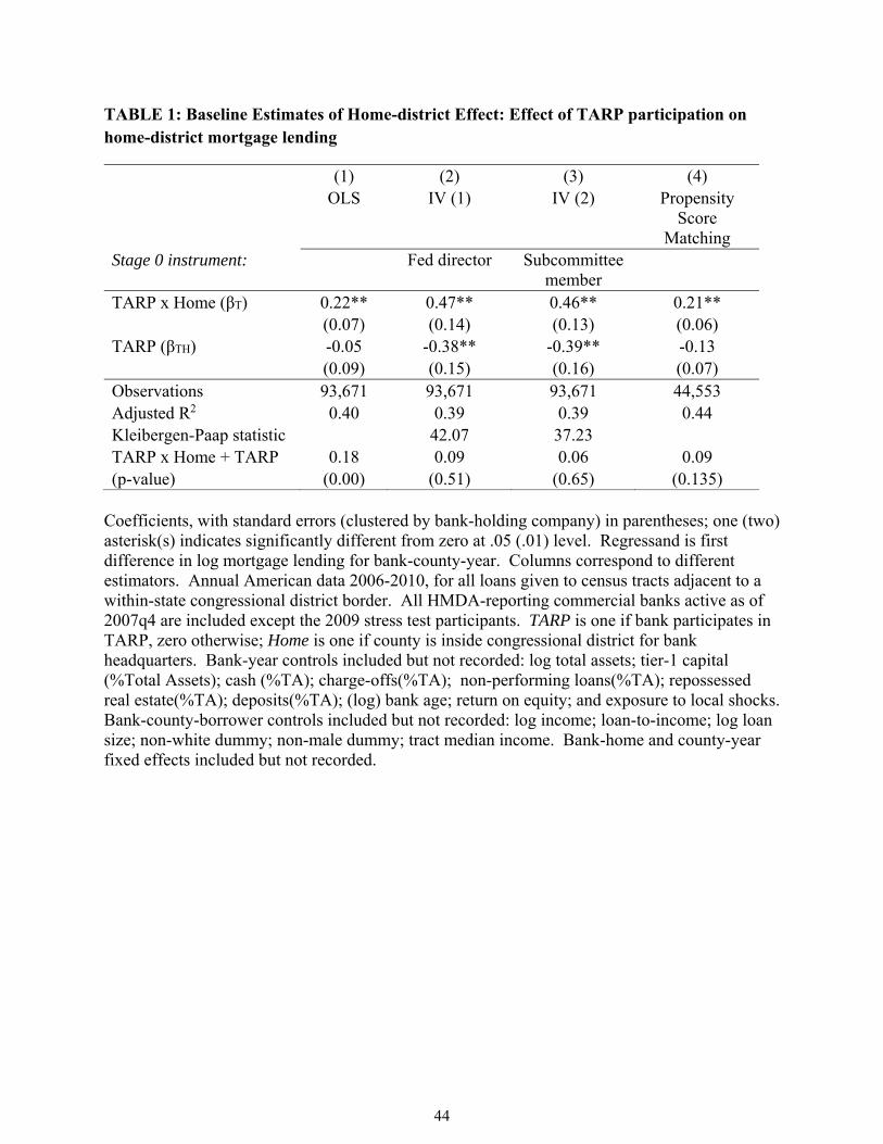
44
TABLE 1: Baseline Estimates of Home-district Effect: Effect of TARP participation on home-district mortgage lending
(1) (2) (3) (4) OLS IV (1) IV (2) Propensity
Score Matching
Stage 0 instrument: Fed director Subcommittee member
TARP x Home (βT) 0.22** 0.47** 0.46** 0.21** (0.07) (0.14) (0.13) (0.06) TARP (βTH) -0.05 -0.38** -0.39** -0.13 (0.09) (0.15) (0.16) (0.07) Observations 93,671 93,671 93,671 44,553 Adjusted R2 0.40 0.39 0.39 0.44 Kleibergen-Paap statistic 42.07 37.23 TARP x Home + TARP 0.18 0.09 0.06 0.09 (p-value) (0.00) (0.51) (0.65) (0.135)
Coefficients, with standard errors (clustered by bank-holding company) in parentheses; one (two) asterisk(s) indicates significantly different from zero at .05 (.01) level. Regressand is first difference in log mortgage lending for bank-county-year. Columns correspond to different estimators. Annual American data 2006-2010, for all loans given to census tracts adjacent to a within-state congressional district border. All HMDA-reporting commercial banks active as of 2007q4 are included except the 2009 stress test participants. TARP is one if bank participates in TARP, zero otherwise; Home is one if county is inside congressional district for bank headquarters. Bank-year controls included but not recorded: log total assets; tier-1 capital (%Total Assets); cash (%TA); charge-offs(%TA); non-performing loans(%TA); repossessed real estate(%TA); deposits(%TA); (log) bank age; return on equity; and exposure to local shocks. Bank-county-borrower controls included but not recorded: log income; loan-to-income; log loan size; non-white dummy; non-male dummy; tract median income. Bank-home and county-year fixed effects included but not recorded.
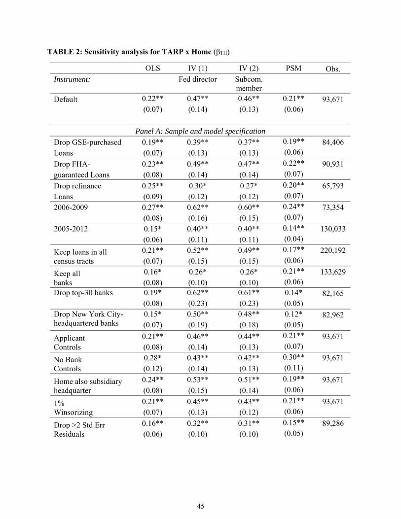
45
TABLE 2: Sensitivity analysis for TARP x Home (βTH)
OLS IV (1) IV (2) PSM Obs. Instrument: Fed director Subcom.
member
Default 0.22** 0.47** 0.46** 0.21** 93,671
(0.07) (0.14) (0.13) (0.06)
Panel A: Sample and model specification
Drop GSE-purchased 0.19** 0.39** 0.37** 0.19** 84,406 Loans (0.07) (0.13) (0.13) (0.06)
Drop FHA- 0.23** 0.49** 0.47** 0.22** 90,931 guaranteed Loans (0.08) (0.14) (0.14) (0.07)
Drop refinance 0.25** 0.30* 0.27* 0.20** 65,793 Loans (0.09) (0.12) (0.12) (0.07) 2006-2009 0.27** 0.62** 0.60** 0.24** 73,354 (0.08) (0.16) (0.15) (0.07) 2005-2012 0.15* 0.40** 0.40** 0.14** 130,033 (0.06) (0.11) (0.11) (0.04)
Keep loans in all census tracts
0.21** 0.52** 0.49** 0.17** 220,192 (0.07) (0.15) (0.15) (0.06)
Keep all banks
0.16* 0.26* 0.26* 0.21** 133,629 (0.08) (0.10) (0.10) (0.06)
Drop top-30 banks 0.19* 0.62** 0.61** 0.14* 82,165 (0.08) (0.23) (0.23) (0.05)
Drop New York City-headquartered banks
0.15* 0.50** 0.48** 0.12* 82,962 (0.07) (0.19) (0.18) (0.05)
Applicant Controls
0.21** 0.46** 0.44** 0.21** 93,671 (0.08) (0.14) (0.13) (0.07)
No Bank Controls
0.28* 0.43** 0.42** 0.30** 93,671 (0.12) (0.14) (0.13) (0.11)
Home also subsidiary headquarter
0.24** 0.53** 0.51** 0.19** 93,671 (0.08) (0.15) (0.14) (0.06)
1% Winsorizing
0.21** 0.45** 0.43** 0.21** 93,671 (0.07) (0.13) (0.12) (0.06)
Drop >2 Std Err Residuals
0.16** 0.32** 0.31** 0.15** 89,286 (0.06) (0.10) (0.10) (0.05)
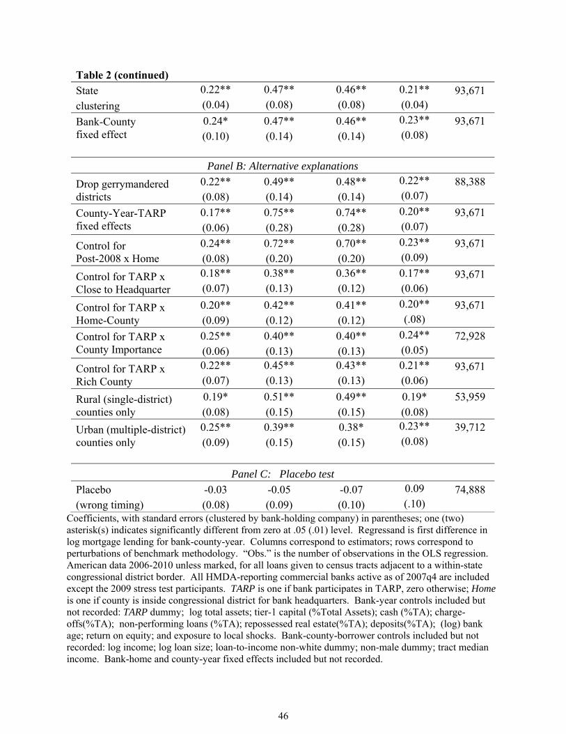
46
Table 2 (continued)
State 0.22** 0.47** 0.46** 0.21** 93,671 clustering (0.04) (0.08) (0.08) (0.04)
Bank-County fixed effect
0.24* 0.47** 0.46** 0.23** 93,671 (0.10) (0.14) (0.14) (0.08)
Panel B: Alternative explanations
Drop gerrymandered districts
0.22** 0.49** 0.48** 0.22** 88,388 (0.08) (0.14) (0.14) (0.07)
County-Year-TARP fixed effects
0.17** 0.75** 0.74** 0.20** 93,671 (0.06) (0.28) (0.28) (0.07)
Control for Post-2008 x Home
0.24** 0.72** 0.70** 0.23** 93,671 (0.08) (0.20) (0.20) (0.09)
Control for TARP x Close to Headquarter
0.18** 0.38** 0.36** 0.17** 93,671 (0.07) (0.13) (0.12) (0.06)
Control for TARP x Home-County
0.20** 0.42** 0.41** 0.20** 93,671 (0.09) (0.12) (0.12) (.08)
Control for TARP x County Importance
0.25** 0.40** 0.40** 0.24** 72,928 (0.06) (0.13) (0.13) (0.05)
Control for TARP x Rich County
0.22** 0.45** 0.43** 0.21** 93,671 (0.07) (0.13) (0.13) (0.06)
Rural (single-district) counties only
0.19* 0.51** 0.49** 0.19* 53,959 (0.08) (0.15) (0.15) (0.08)
Urban (multiple-district) counties only
0.25** 0.39** 0.38* 0.23** 39,712 (0.09) (0.15) (0.15) (0.08)
Panel C: Placebo test
Placebo -0.03 -0.05 -0.07 0.09 74,888 (wrong timing) (0.08) (0.09) (0.10) (.10)
Coefficients, with standard errors (clustered by bank-holding company) in parentheses; one (two) asterisk(s) indicates significantly different from zero at .05 (.01) level. Regressand is first difference in log mortgage lending for bank-county-year. Columns correspond to estimators; rows correspond to perturbations of benchmark methodology. “Obs.” is the number of observations in the OLS regression. American data 2006-2010 unless marked, for all loans given to census tracts adjacent to a within-state congressional district border. All HMDA-reporting commercial banks active as of 2007q4 are included except the 2009 stress test participants. TARP is one if bank participates in TARP, zero otherwise; Home is one if county is inside congressional district for bank headquarters. Bank-year controls included but not recorded: TARP dummy; log total assets; tier-1 capital (%Total Assets); cash (%TA); charge-offs(%TA); non-performing loans (%TA); repossessed real estate(%TA); deposits(%TA); (log) bank age; return on equity; and exposure to local shocks. Bank-county-borrower controls included but not recorded: log income; log loan size; loan-to-income non-white dummy; non-male dummy; tract median income. Bank-home and county-year fixed effects included but not recorded.
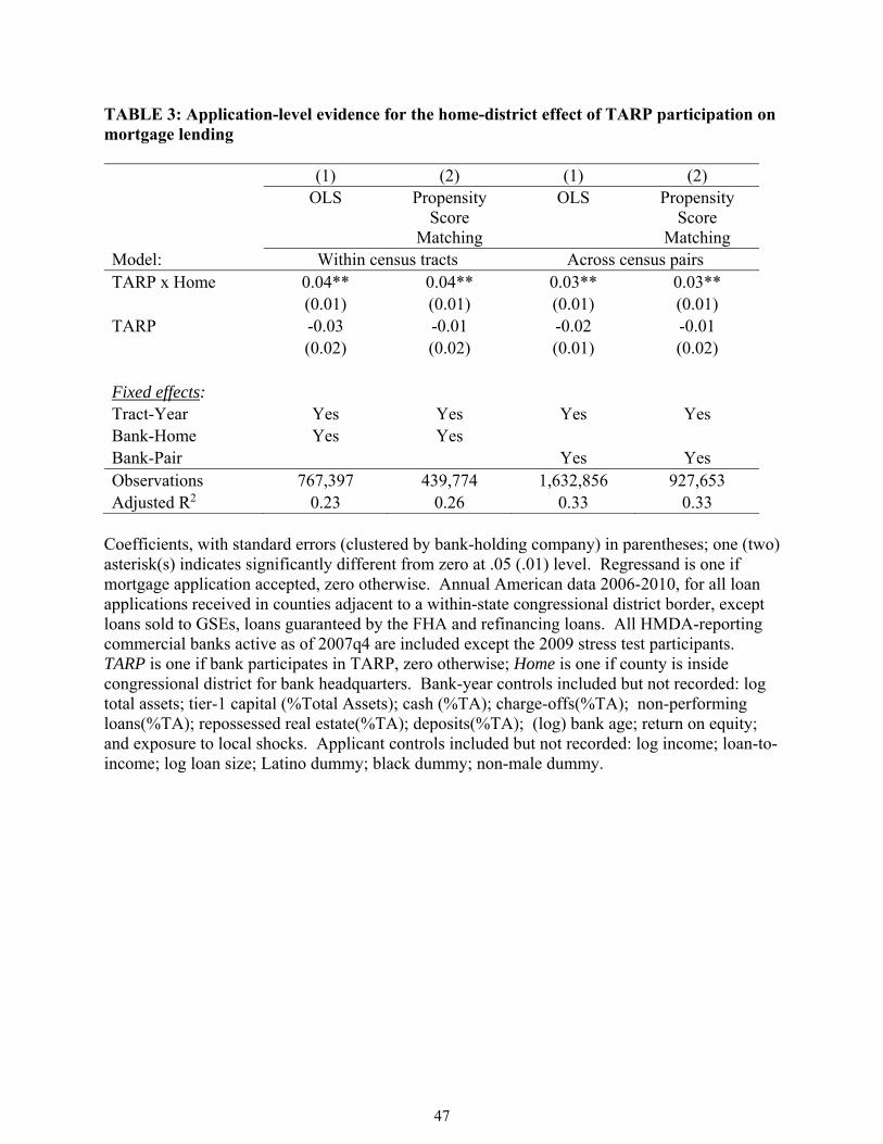
47
TABLE 3: Application-level evidence for the home-district effect of TARP participation on mortgage lending (1) (2) (1) (2) OLS Propensity
Score Matching
OLS Propensity Score
Matching Model: Within census tracts Across census pairs TARP x Home 0.04** 0.04** 0.03** 0.03** (0.01) (0.01) (0.01) (0.01) TARP -0.03 -0.01 -0.02 -0.01 (0.02) (0.02) (0.01) (0.02) Fixed effects: Tract-Year Yes Yes Yes Yes Bank-Home Yes Yes Bank-Pair Yes Yes Observations 767,397 439,774 1,632,856 927,653 Adjusted R2 0.23 0.26 0.33 0.33
Coefficients, with standard errors (clustered by bank-holding company) in parentheses; one (two) asterisk(s) indicates significantly different from zero at .05 (.01) level. Regressand is one if mortgage application accepted, zero otherwise. Annual American data 2006-2010, for all loan applications received in counties adjacent to a within-state congressional district border, except loans sold to GSEs, loans guaranteed by the FHA and refinancing loans. All HMDA-reporting commercial banks active as of 2007q4 are included except the 2009 stress test participants. TARP is one if bank participates in TARP, zero otherwise; Home is one if county is inside congressional district for bank headquarters. Bank-year controls included but not recorded: log total assets; tier-1 capital (%Total Assets); cash (%TA); charge-offs(%TA); non-performing loans(%TA); repossessed real estate(%TA); deposits(%TA); (log) bank age; return on equity; and exposure to local shocks. Applicant controls included but not recorded: log income; loan-to-income; log loan size; Latino dummy; black dummy; non-male dummy.

48
TABLE 4: Home-district effect of TARP participation on small business lending
(1) (2) (3) (4) OLS IV (1) IV (2) Propensity
Score Matching
Stage 0 instrument: Fed director Subcommittee member
TARP x Home 0.26 0.48* 0.50* 0.21* (0.14) (0.21) (0.22) (0.10) TARP 0.05 -0.34 -0.27 0.03 (0.16) (0.21) (0.22) (0.09) Observations 43,019 42,896 42,896 25,868 Adjusted R2 0.25 0.03 0.03 0.28
Coefficients, with standard errors (clustered by bank-holding company) in parentheses; one (two) asterisk(s) indicates significantly different from zero at .05 (.01) level. Regressand is small business lending (log) growth. Annual American data 2006-2010, includes all loans given out in counties adjacent to a within-state congressional district border. All HMDA-reporting commercial banks active as of 2007q4 are included except the 2009 stress test participants. TARP is one if bank participates in TARP, zero otherwise; Home is one if county is inside congressional district for bank headquarters. Bank-year controls included but not recorded: log total assets; tier-1 capital (%Total Assets); cash (%TA); charge-offs(%TA); non-performing loans(%TA); repossessed real estate(%TA); deposits(%TA); (log) bank age; return on equity; and exposure to local shocks. Bank-home and county-year fixed effects included but not recorded.
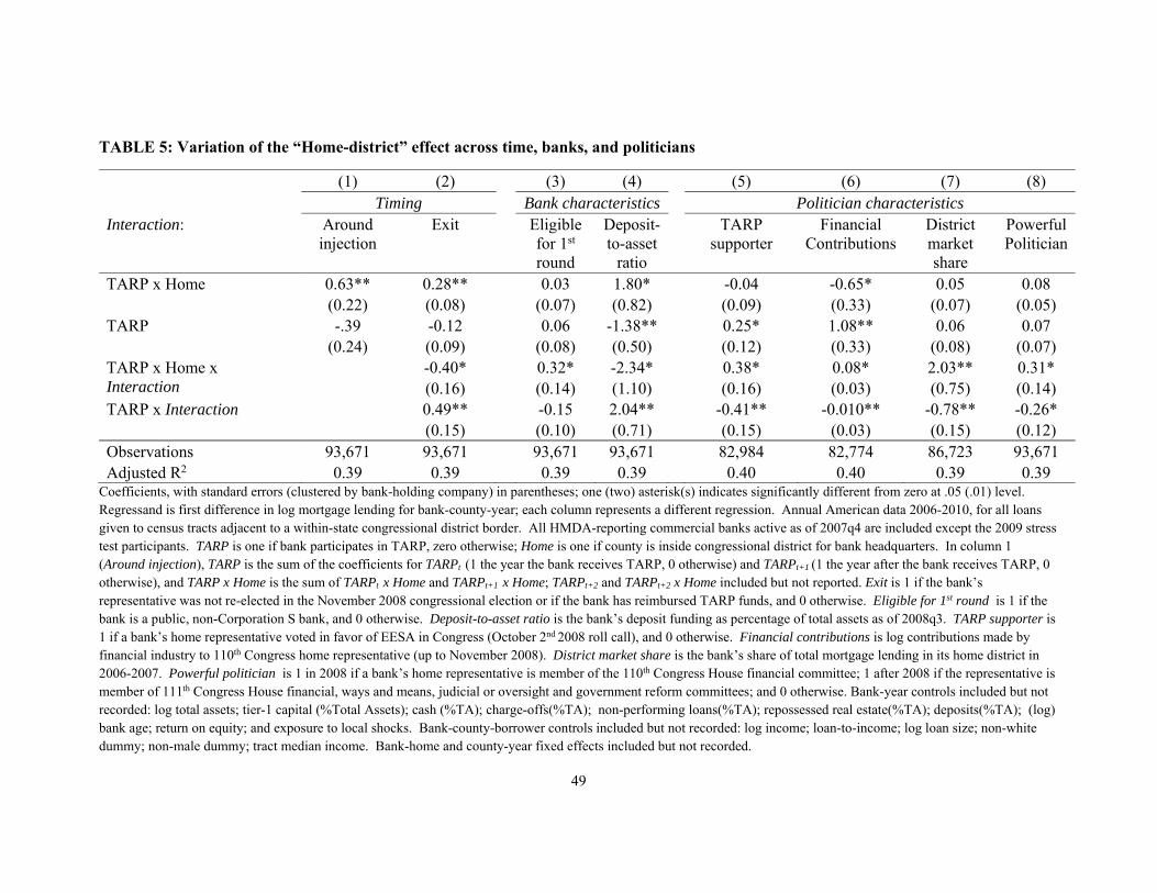
49
TABLE 5: Variation of the “Home-district” effect across time, banks, and politicians
Coefficients, with standard errors (clustered by bank-holding company) in parentheses; one (two) asterisk(s) indicates significantly different from zero at .05 (.01) level. Regressand is first difference in log mortgage lending for bank-county-year; each column represents a different regression. Annual American data 2006-2010, for all loans given to census tracts adjacent to a within-state congressional district border. All HMDA-reporting commercial banks active as of 2007q4 are included except the 2009 stress test participants. TARP is one if bank participates in TARP, zero otherwise; Home is one if county is inside congressional district for bank headquarters. In column 1 (Around injection), TARP is the sum of the coefficients for TARPt (1 the year the bank receives TARP, 0 otherwise) and TARPt+1 (1 the year after the bank receives TARP, 0 otherwise), and TARP x Home is the sum of TARPt x Home and TARPt+1 x Home; TARPt+2 and TARPt+2 x Home included but not reported. Exit is 1 if the bank’s representative was not re-elected in the November 2008 congressional election or if the bank has reimbursed TARP funds, and 0 otherwise. Eligible for 1st round is 1 if the bank is a public, non-Corporation S bank, and 0 otherwise. Deposit-to-asset ratio is the bank’s deposit funding as percentage of total assets as of 2008q3. TARP supporter is 1 if a bank’s home representative voted in favor of EESA in Congress (October 2nd 2008 roll call), and 0 otherwise. Financial contributions is log contributions made by financial industry to 110th Congress home representative (up to November 2008). District market share is the bank’s share of total mortgage lending in its home district in 2006-2007. Powerful politician is 1 in 2008 if a bank’s home representative is member of the 110th Congress House financial committee; 1 after 2008 if the representative is member of 111th Congress House financial, ways and means, judicial or oversight and government reform committees; and 0 otherwise. Bank-year controls included but not recorded: log total assets; tier-1 capital (%Total Assets); cash (%TA); charge-offs(%TA); non-performing loans(%TA); repossessed real estate(%TA); deposits(%TA); (log) bank age; return on equity; and exposure to local shocks. Bank-county-borrower controls included but not recorded: log income; loan-to-income; log loan size; non-white dummy; non-male dummy; tract median income. Bank-home and county-year fixed effects included but not recorded.
(1) (2) (3) (4) (5) (6) (7) (8) Timing Bank characteristics Politician characteristics Interaction: Around
injection Exit Eligible
for 1st round
Deposit-to-asset
ratio
TARP supporter
Financial Contributions
District market share
Powerful Politician
TARP x Home 0.63** 0.28** 0.03 1.80* -0.04 -0.65* 0.05 0.08 (0.22) (0.08) (0.07) (0.82) (0.09) (0.33) (0.07) (0.05) TARP -.39 -0.12 0.06 -1.38** 0.25* 1.08** 0.06 0.07 (0.24) (0.09) (0.08) (0.50) (0.12) (0.33) (0.08) (0.07) TARP x Home x Interaction
-0.40* 0.32* -2.34* 0.38* 0.08* 2.03** 0.31* (0.16) (0.14) (1.10) (0.16) (0.03) (0.75) (0.14)
TARP x Interaction 0.49** -0.15 2.04** -0.41** -0.010** -0.78** -0.26* (0.15) (0.10) (0.71) (0.15) (0.03) (0.15) (0.12)
Observations 93,671 93,671 93,671 93,671 82,984 82,774 86,723 93,671 Adjusted R2 0.39 0.39 0.39 0.39 0.40 0.40 0.39 0.39
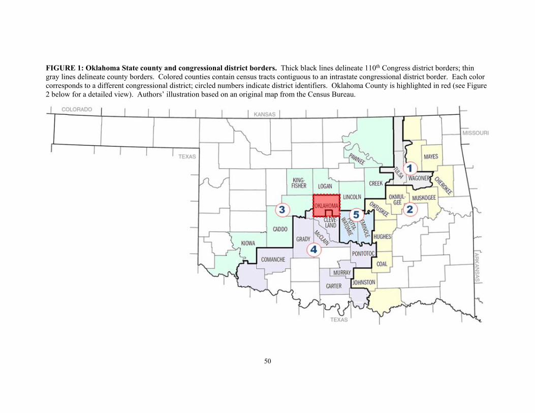
50
FIGURE 1: Oklahoma State county and congressional district borders. Thick black lines delineate 110th Congress district borders; thin gray lines delineate county borders. Colored counties contain census tracts contiguous to an intrastate congressional district border. Each color corresponds to a different congressional district; circled numbers indicate district identifiers. Oklahoma County is highlighted in red (see Figure 2 below for a detailed view). Authors’ illustration based on an original map from the Census Bureau.
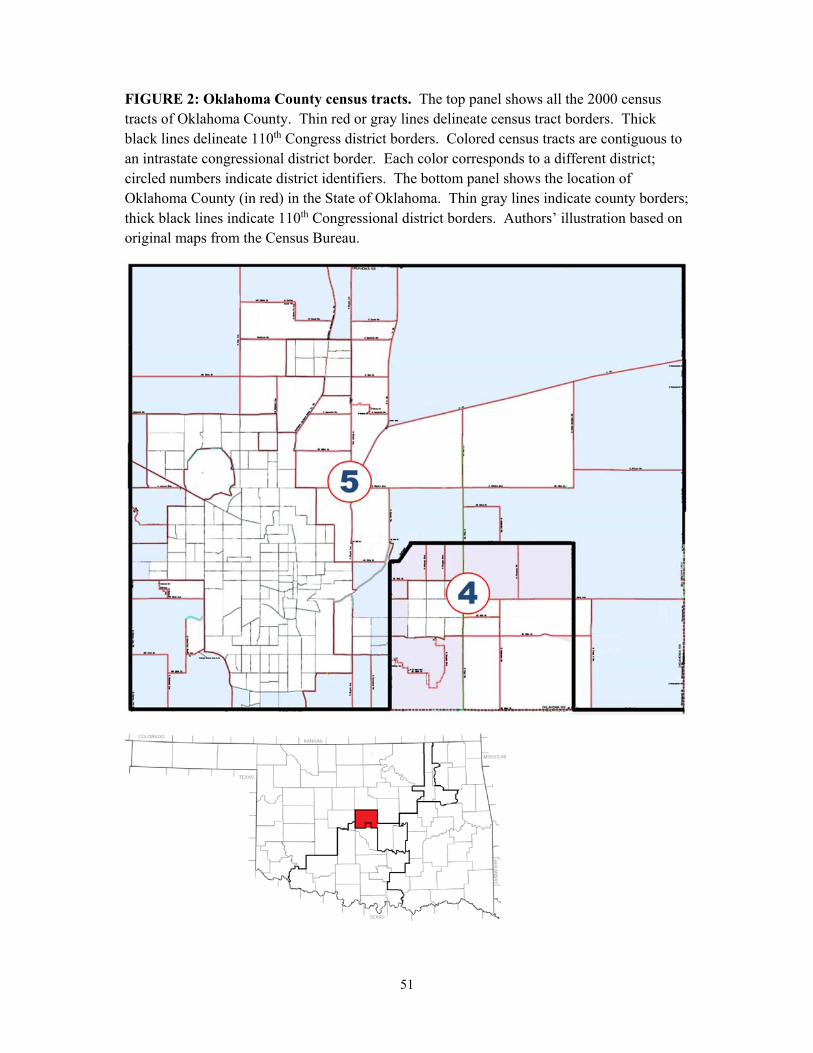
51
FIGURE 2: Oklahoma County census tracts. The top panel shows all the 2000 census tracts of Oklahoma County. Thin red or gray lines delineate census tract borders. Thick black lines delineate 110th Congress district borders. Colored census tracts are contiguous to an intrastate congressional district border. Each color corresponds to a different district; circled numbers indicate district identifiers. The bottom panel shows the location of Oklahoma County (in red) in the State of Oklahoma. Thin gray lines indicate county borders; thick black lines indicate 110th Congressional district borders. Authors’ illustration based on original maps from the Census Bureau.
52
Appendix A1: Impact of Discontinuity Strategy on the Sample
The key idea of the discontinuity component of our identification strategy is to
include in the benchmark sample only mortgages given in census tracts adjacent to an
intrastate congressional district border. This section discusses how this approach changes the
sample compared to the full sample obtained when using all data.
Panel A in Table A1 shows that 12,007 of the 65,310 American census tracts are
contiguous to an intrastate district border; 81.6% of tracts are thus left out of the benchmark
sample. But since we collapse data by bank-county-year, the loss of observations compared
to the sample obtain when collapsing the full sample is proportionately smaller.65 Panel B of
Table A1 illustrates this fact; the benchmark has 93,671 bank-county-year observations,
against 219,072 for the full sample.
The difference between the two samples reflects two sources of data loss. First, we
drop data from all counties that have no contiguous tract whatsoever, such as the non-shaded
Oklahoma counties in Figure 1. Only 2,141 of 3,636 American counties (59%) contain at
least one contiguous tract and are thus included in the benchmark sample.66 The other
counties are left out of the benchmark sample.
Second, for those counties that are included in the benchmark sample, we lose data
from all non-contiguous tracts within that county; see for instance the non-shaded Oklahoma
City county tracts in Figure 2. For the mean bank-county-year observation, 52% of the
lending volume comes from contiguous tracts and is thus taken into account when we
compute annual bank-county mortgage growth. The other (48%) loans are not taken into
account in the benchmark sample. This loss of data makes it less likely that there are two
65 A hypothetical county with 100 tracts would be included in the benchmark sample even if only one of its tracts is a contiguous one. However, the benchmark sample would use only around 1% of the lending volume in that county to compute bank-county-year mortgage growth, whereas the full sample would use 100% of it. 66 The total number of counties in our sample is higher than the official number of counties (3,143) since we split multiple-district counties into district-counties.
53
consecutive non-zero lending for a given bank-county-year combination, and that the latter is
thus included in the benchmark sample.
Does the discontinuity approach create a selection bias and undermines the external
validity of our results? Panel C in Table A1 reports summary statistics for the bank-county
variables in the benchmark and full samples. Annual mortgage growth is not statistically
different across the two samples; lending dynamics in the baseline sample are thus
representative of those of the full sample. Borrower controls are statistically different across
the two samples, but differences seem economically small. For instance, 6% of loans go to
non-white borrowers in the benchmark sample, against 6.3% in the full sample.67 Robustness
checks discussed in section 5 confirm that we obtain quantitatively similar results when using
the full sample.
67 This possibly reflects the fact that rural counties are less likely to contain contiguous tracts and thus to be included.

54
Table A1: Comparing the Benchmark Discontinuity (contiguous census tracts only) and Full Samples (all census tracts)
(1) (2) (3) (4)
Panel A: Total number of U.S. census tracts
All tracts Contiguous tracts
Number of census tracts 65,310 12,007
Panel B: Sample characteristics
All tracts Contiguous tracts
Number of bank-county observations 219,072 93,671
Number of banks 3,395 2,699
Number of counties 3,636 2,141
% included loan volume (mean year-county-bank obs.)
100% 52.0%
Panel C: Bank-county mean characteristics
All tracts Contiguous tracts Diff t-test
Δ (log) mortgage lending 0.018 0.015 0.004 -0.004
(Log) borrower income 4.511 4.475 0.036 0.046**
(Log) loan size 4.949 4.935 0.014 0.083**
Borrower tract (log) median income 4.646 4.683 -0.037 0.002**
Borrower loan-to-income 2.081 2.099 -0.018 0.066**
Non-male dummy 0.193 0.192 0.001 -0.000
Non-white dummy 0.063 0.060 0.003 0.002** Panel A reports the total number of 2000 US Census tracts (column 1), and the number of these tracts contiguous to an intrastate 110th Congress district border (column 2). Panel B reports key characteristics of the benchmark sample (containing only loans in contiguous tracts) and full samples (containing loans in all tracts). Annual American data 2006-2010. Panel C reports the average of bank-county-year variable in the benchmark sample (column 1) and full sample (column 2); column 3 reports the difference between these means. Column 4 reports the paired t-test for mean difference between the value of a variable in the benchmark sample and the corresponding observation in the full sample; one (two) asterisk(s) indicates mean equality can be rejected at .05 (.01) significance level. Raw (loan-level) data are aggregated by year and county (district for multiple-district counties) in the two samples. Both samples cover all HMDA-reporting commercial banks active as of 2007Q4 are included except the 2009 stress test participants.
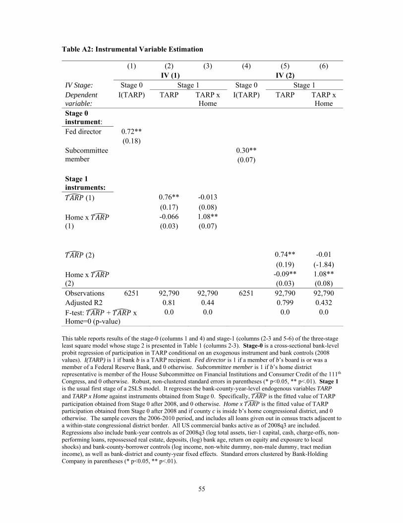
55
Table A2: Instrumental Variable Estimation
(1) (2) (3) (4) (5) (6) IV (1) IV (2) IV Stage: Stage 0 Stage 1 Stage 0 Stage 1 Dependent variable:
I(TARP) TARP TARP x Home
I(TARP) TARP TARP x Home
Stage 0 instrument:
Fed director 0.72** (0.18)
Subcommittee member
0.30** (0.07)
Stage 1 instruments:
(1) 0.76** -0.013 (0.17) (0.08) Home x (1)
-0.066 1.08** (0.03) (0.07)
(2) 0.74** -0.01 (0.19) (-1.84) Home x (2)
-0.09** 1.08** (0.03) (0.08)
Observations 6251 92,790 92,790 6251 92,790 92,790 Adjusted R2 0.81 0.44 0.799 0.432 F-test: + x Home=0 (p-value)
0.0 0.0 0.0 0.0
This table reports results of the stage-0 (columns 1 and 4) and stage-1 (columns (2-3 and 5-6) of the three-stage least square model whose stage 2 is presented in Table 1 (columns 2-3). Stage-0 is a cross-sectional bank-level probit regression of participation in TARP conditional on an exogenous instrument and bank controls (2008 values). I(TARP) is 1 if bank b is a TARP recipient. Fed director is 1 if a member of b’s board is or was a member of a Federal Reserve Bank, and 0 otherwise. Subcommittee member is 1 if b’s home district representative is member of the House Subcommittee on Financial Institutions and Consumer Credit of the 111th Congress, and 0 otherwise. Robust, non-clustered standard errors in parentheses (* p<0.05, ** p<.01). Stage 1 is the usual first stage of a 2SLS model. It regresses the bank-county-year-level endogenous variables TARP and TARP x Home against instruments obtained from Stage 0. Specifically, is the fitted value of TARP participation obtained from Stage 0 after 2008, and 0 otherwise. Home x is the fitted value of TARP participation obtained from Stage 0 after 2008 and if county c is inside b’s home congressional district, and 0 otherwise. The sample covers the 2006-2010 period, and includes all loans given out in census tracts adjacent to a within-state congressional district border. All US commercial banks active as of 2008q3 are included. Regressions also include bank-year controls as of 2008q3 (log total assets, tier-1 capital, cash, charge-offs, non-performing loans, repossessed real estate, deposits, (log) bank age, return on equity and exposure to local shocks) and bank-county-borrower controls (log income, non-white dummy, non-male dummy, tract median income), as well as bank-district and county-year fixed effects. Standard errors clustered by Bank-Holding Company in parentheses (* p<0.05, ** p<.01).
56
Appendix A2: Summary Descriptive Statistics and Parallel Trends
Table A3 provides summary statistics for the benchmark sample. (Log) mortgage
lending grows by 1.5% for the average bank-county-year. 22% of these observations concern
banks in their home district; 21% capture banks in the TARP program, around 10% of which
concern home-district lending.
Our main interest is to estimate whether TARP participants’ lending growth is higher
in their home district vs. elsewhere, compared to non-participants. Figure A1 provides
suggestive visual evidence for this “home-district effect”; it plots average bank-county annual
mortgage growth for participants vs. other banks in counties outside their home districts
(panel A) and inside it (panel B). The most striking pattern is that TARP participants
substantially cut lending outside the home district during TARP years (2008-2009) while
non-participants increase lending. Meanwhile, home-district lending seems much less
affected: participants and non-participants both keep on increasing lending during the TARP
years. Trends for both groups seem to converge at the end of the sample (2010).
Section 5 in the main text confirms the existence of a significant “home-district
effect” in a regression analysis; we interpret this effect as a consequence of participation in
TARP. For this inference to be valid, participants’ home- and non-home district lending
growth should have followed a trend similar to non-participants absent TARP. Panel A in
Figure A1 shows that this parallel trends assumption is satisfied for non-home district
lending: trends before TARP (2006-2007) are almost indistinguishable outside the home
district. Trends seem roughly comparable in the home district as well (panel B). However
we cannot rule out that these trends are statistically different on the basis of this graph only.
Of course, the plots of Figure A1 are simple averages, not controlling for any of the
many influences on mortgage lending that vary by area, bank, and time. Still, three tests
suggest that our finding is attributable to TARP, not differential trends in lending growth.
57
First, future participation in TARP does not have any significant effect in the pre-TARP
period (see section 5). Second, baseline results do not change when we match participants
with non-participants based on their pre-TARP home-lending growth trend (see Appendix
A3). Finally, a robustness check in section 5 suggests that the home-district effect is reversed
once participants exit the program.
Figure A1 suggests another possible caveat of our experiment. Panel A shows that in
2008, non-home lending trend changes for non-participants as well. This suggests that
developments parallel to TARP might have changed all banks’ incentives to lend outside of
their home district. In the main text, we conjecture that this reflects a general crisis-time
retrenchment away from arm’s length lending following the collapse of non-agency
securitization markets. A robustness check in section 5 shows that controlling for this effect
does not change our estimate of the home-district effect.

58
Table A3: Summary Statistics for the Benchmark Sample
(1) (2)
Mean Std. Dev.
Panel A: Bank-year variables
TARP 0.212 0.41(Log) total assets 14.10 2.76Tier-1 capital (% Total assets) 0.08 0.03Cash (% Total assets) 0.02 0.02Charge-offs (% Total assets) 0.01 0.01Repossessed real estate (% Total assets) 0.00 0.01Deposits (% Total assets) 0.73 0.14Non-performing loans (% Total assets) 0.02 0.02(Log) bank age 66.55 42.33Return on equity 0.06 0.15Exposure to local shocks -0.16 1.62
Panel B: Bank-county-year variables
Δ (log) mortgage lending 0.015 1.12Home 0.22 0.41TARP x Home 0.020 0.14Borrower loan-to-income 2.10 1.07(Log) borrower income 4.48 0.61(Log) loan size 4.94 0.82Borrower tract (log) median income 4.68 0.27Non-white dummy 0.06 0.18Non-male dummy 0.19 0.26
Panel C: Additional bank-level variables
Exit 0.13 0.34Eligible for 1st round 0.39 0.49Deposit-to-asset ratio 0.72 0.14TARP supporter 0.63 0.48Financial contributions 11.99 0.98District market share 0.09 0.14Powerful politician 0.35 0.48
This table reports the mean (column 1) and standard deviation (column 2) of variables of the main regression model (1) for all observations included in the benchmark sample. Annual American data 2006-2010, for all loans given to census tracts adjacent to a within-state congressional district border. All HMDA-reporting commercial banks active as of 2007q4 are included except the 2009 stress test participants. TARP is one if bank participates in TARP, zero otherwise; Home is one if county is inside congressional district for bank headquarters. See section 4 (bank-year and bank-county-year variables) and section 6 (additional bank-level variables) for other variable definitions.
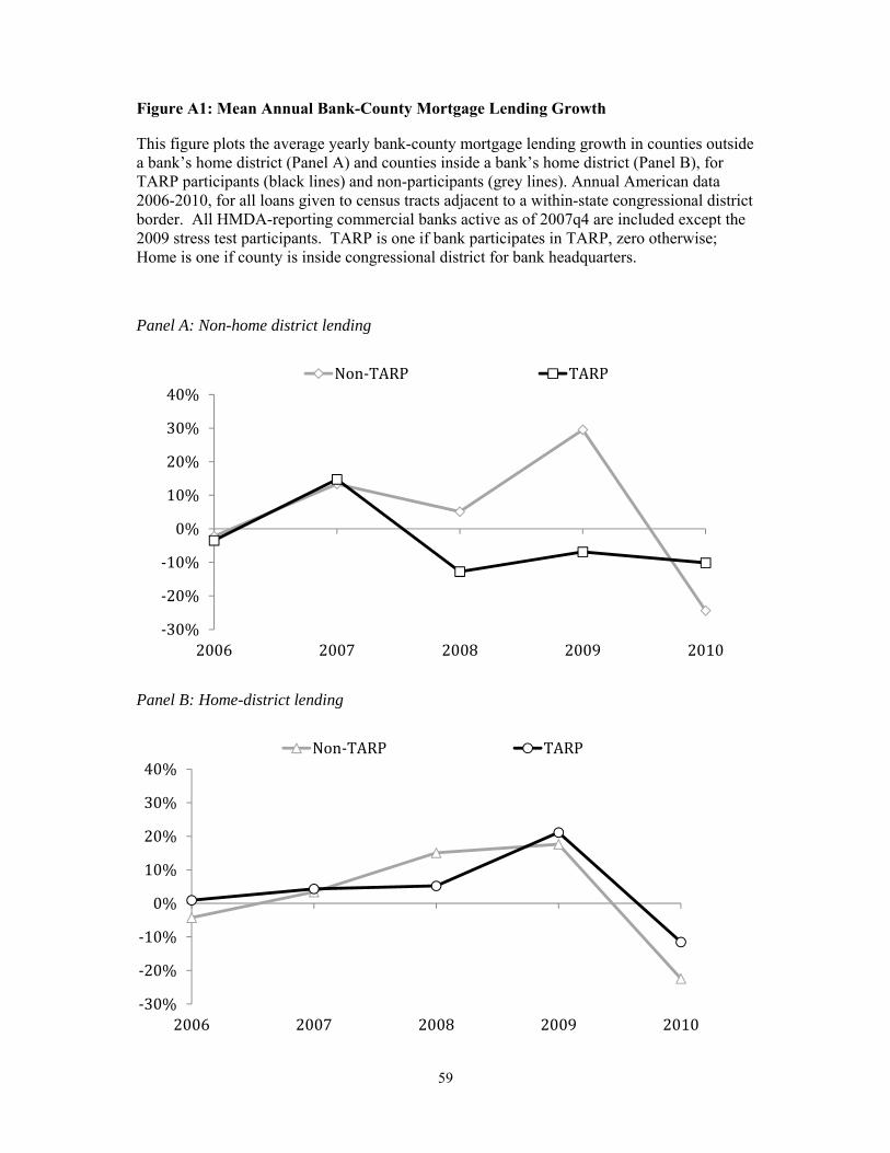
59
Figure A1: Mean Annual Bank-County Mortgage Lending Growth
This figure plots the average yearly bank-county mortgage lending growth in counties outside a bank’s home district (Panel A) and counties inside a bank’s home district (Panel B), for TARP participants (black lines) and non-participants (grey lines). Annual American data 2006-2010, for all loans given to census tracts adjacent to a within-state congressional district border. All HMDA-reporting commercial banks active as of 2007q4 are included except the 2009 stress test participants. TARP is one if bank participates in TARP, zero otherwise; Home is one if county is inside congressional district for bank headquarters.
Panel A: Non-home district lending
Panel B: Home-district lending
‐30%
‐20%
‐10%
0%
10%
20%
30%
40%
2006 2007 2008 2009 2010
Non‐TARP TARP
‐30%
‐20%
‐10%
0%
10%
20%
30%
40%
2006 2007 2008 2009 2010
Non‐TARP TARP

60
Appendix A3: Heterogeneity between banks and districts
Our main test compares TARP and non-TARP banks’ lending growth inside and
outside their home-district counties. This difference-in-difference-in-difference approach
diminishes the possibility that our main result is biased because TARP and non-TARP banks
or home-district and non-home district counties are heterogeneous in other dimensions than
their susceptibility to political influences after TARP. This section provides additional
evidence in support of this claim.
Heterogeneity between banks
We first investigate differences between TARP and non-TARP banks. In the paper,
we explore these heterogeneities through the baseline propensity-score matching exercise
(column 4 in Tables 1 and 2). This exercise matches participants and non-participants based
on a combination of pre-TARP bank-level characteristics, as captured by their propensity to
participate. Still, recipients and non-recipients could differ along individual pre-TARP
characteristics. For instance low-capital banks could be more prone to participate and to face
political pressure irrespective of participation.
We thus successively match participants and non-participants based on every control
variable in our baseline model as measured before TARP (2007).68 In addition to these
variables, we match banks based on (i) the trend in home-district lending growth (measured
as the difference between mean 2007 and 2006 mortgage growth) and (ii) their volume of
home-district lending as percentage of total lending. The former matching controls for
possible differences in pre-TARP home-district growth trend suggested by visual inspection
of parallel trends (Figure A1). The latter matching controls for the possibility that TARP
banks are larger and thus less dependent on their home-district markets.
68 The methodology largely follows Cohn and Wardlaw (2016).

61
Table A4 reports the results of this analysis. Columns 1 to 3 suggest that matching
successfully erase differences across participants and non-participants in all dimensions but
size and age. However, the remaining difference in these two cases looks economically
negligible. Columns 4 and 5 report the size and standard error of the main coefficient of
interest TARP x Home as obtained when running the baseline regression using the respective
matched samples. The economic magnitude and statistical significance of the parameter are
stable and very similar to the baseline result in all cases. This suggests that differences in
observable bank-level and bank-home-district characteristics across recipients and non-
recipients do not explain our baseline results.
Heterogeneity between districts
We then investigate differences between home-district and non-home district
counties. Banks may tend to be headquartered in downtown areas. These areas can either be
more affluent or more deprived than contiguous areas, depending on the city. However, these
heterogeneities should only bias our results if they are specific to TARP participants while
they are on the program, because of our difference-in-difference-in-difference approach.69
We explore several variants of this hypothesis in Table A5. Specifically, we repeat
the baseline regression (1) while controlling for an additional county characteristic and its
interaction with TARP. We consider six different characteristics, all measured as county
averages in 2006-2007. Colum 1 reports the parameter estimate for TARP x Home when
each of these additional variables is controlled for. The parameter estimate barely changes at
all across all six regressions. This confirms that our approach is not sensitive to non-political
heterogeneities across districts.70
69 For instance, TARP banks could be more prone to “fly” once on the program if they are headquartered in affluent areas and surrounded by deprived suburbs. 70 We reach a similar conclusion when alternatively coding the county characteristic as a dummy – one if above median for a given bank, 0 otherwise.
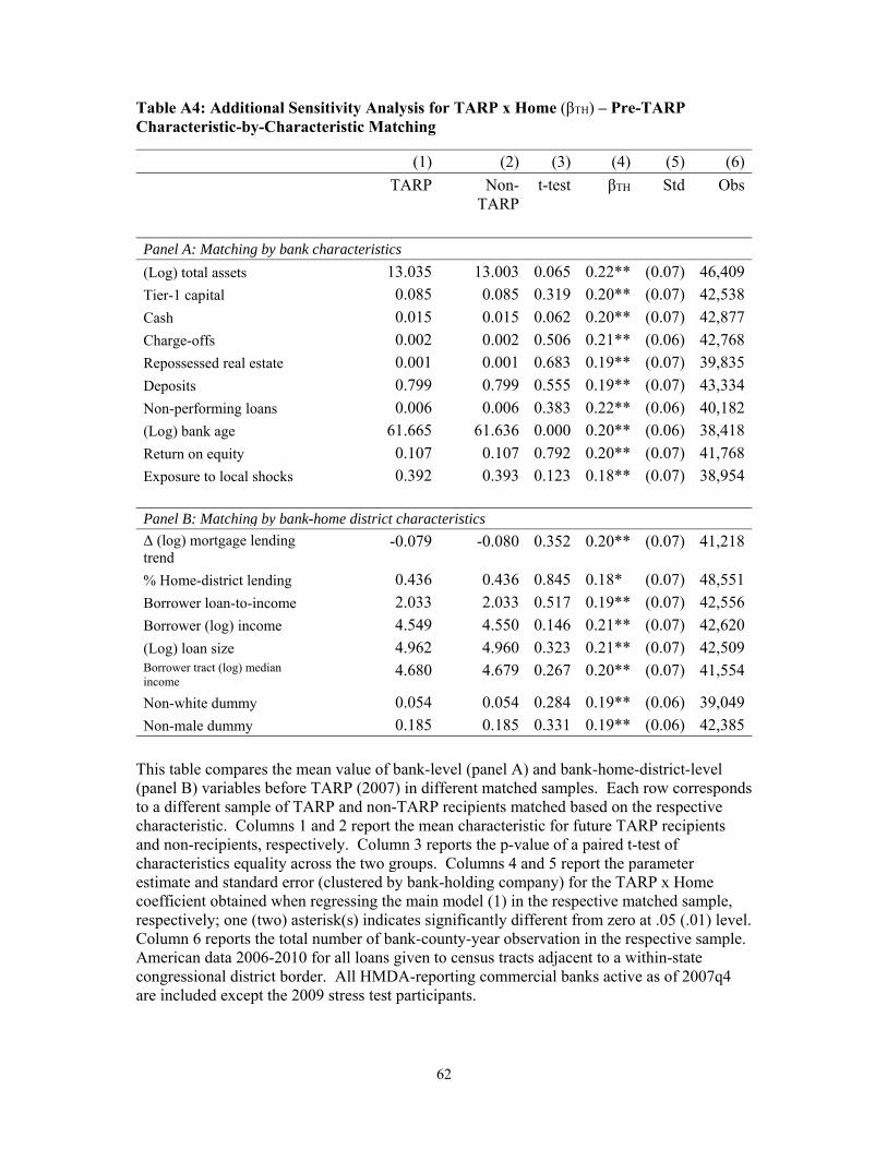
62
Table A4: Additional Sensitivity Analysis for TARP x Home (βTH) – Pre-TARP Characteristic-by-Characteristic Matching
(1) (2) (3) (4) (5) (6)
TARP Non-TARP
t-test βTH Std Obs
Panel A: Matching by bank characteristics
(Log) total assets 13.035 13.003 0.065 0.22** (0.07) 46,409
Tier-1 capital 0.085 0.085 0.319 0.20** (0.07) 42,538
Cash 0.015 0.015 0.062 0.20** (0.07) 42,877
Charge-offs 0.002 0.002 0.506 0.21** (0.06) 42,768
Repossessed real estate 0.001 0.001 0.683 0.19** (0.07) 39,835
Deposits 0.799 0.799 0.555 0.19** (0.07) 43,334
Non-performing loans 0.006 0.006 0.383 0.22** (0.06) 40,182
(Log) bank age 61.665 61.636 0.000 0.20** (0.06) 38,418
Return on equity 0.107 0.107 0.792 0.20** (0.07) 41,768
Exposure to local shocks 0.392 0.393 0.123 0.18** (0.07) 38,954
Panel B: Matching by bank-home district characteristics
Δ (log) mortgage lending trend
-0.079 -0.080 0.352 0.20** (0.07) 41,218
% Home-district lending 0.436 0.436 0.845 0.18* (0.07) 48,551
Borrower loan-to-income 2.033 2.033 0.517 0.19** (0.07) 42,556
Borrower (log) income 4.549 4.550 0.146 0.21** (0.07) 42,620
(Log) loan size 4.962 4.960 0.323 0.21** (0.07) 42,509Borrower tract (log) median income
4.680 4.679 0.267 0.20** (0.07) 41,554
Non-white dummy 0.054 0.054 0.284 0.19** (0.06) 39,049
Non-male dummy 0.185 0.185 0.331 0.19** (0.06) 42,385
This table compares the mean value of bank-level (panel A) and bank-home-district-level (panel B) variables before TARP (2007) in different matched samples. Each row corresponds to a different sample of TARP and non-TARP recipients matched based on the respective characteristic. Columns 1 and 2 report the mean characteristic for future TARP recipients and non-recipients, respectively. Column 3 reports the p-value of a paired t-test of characteristics equality across the two groups. Columns 4 and 5 report the parameter estimate and standard error (clustered by bank-holding company) for the TARP x Home coefficient obtained when regressing the main model (1) in the respective matched sample, respectively; one (two) asterisk(s) indicates significantly different from zero at .05 (.01) level. Column 6 reports the total number of bank-county-year observation in the respective sample. American data 2006-2010 for all loans given to census tracts adjacent to a within-state congressional district border. All HMDA-reporting commercial banks active as of 2007q4 are included except the 2009 stress test participants.
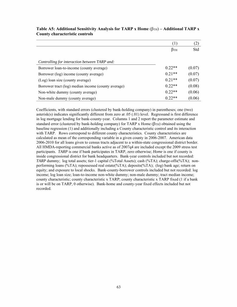
63
Table A5: Additional Sensitivity Analysis for TARP x Home (βTH) – Additional TARP x County characteristic controls
(1) (2)
βTH Std
Controlling for interaction between TARP and:
Borrower loan-to-income (county average) 0.22** (0.07)
Borrower (log) income (county average) 0.21** (0.07)
(Log) loan size (county average) 0.21** (0.07)
Borrower tract (log) median income (county average) 0.22** (0.08)
Non-white dummy (county average) 0.22** (0.06)
Non-male dummy (county average) 0.22** (0.06)
Coefficients, with standard errors (clustered by bank-holding company) in parentheses; one (two) asterisk(s) indicates significantly different from zero at .05 (.01) level. Regressand is first difference in log mortgage lending for bank-county-year. Columns 1 and 2 report the parameter estimate and standard error (clustered by bank-holding company) for TARP x Home (βTH) obtained using the baseline regression (1) and additionally including a County characteristic control and its interaction with TARP. Rows correspond to different county characteristics. County characteristics are calculated as mean of the corresponding variable in a given county in 2006-2007. American data 2006-2010 for all loans given to census tracts adjacent to a within-state congressional district border. All HMDA-reporting commercial banks active as of 2007q4 are included except the 2009 stress test participants. TARP is one if bank participates in TARP, zero otherwise; Home is one if county is inside congressional district for bank headquarters. Bank-year controls included but not recorded: TARP dummy; log total assets; tier-1 capital (%Total Assets); cash (%TA); charge-offs(%TA); non-performing loans (%TA); repossessed real estate(%TA); deposits(%TA); (log) bank age; return on equity; and exposure to local shocks. Bank-county-borrower controls included but not recorded: log income; log loan size; loan-to-income non-white dummy; non-male dummy; tract median income; county characteristic; county characteristic x TARP; county characteristic x TARP fixed (1 if a bank is or will be on TARP, 0 otherwise). Bank-home and county-year fixed effects included but not recorded.
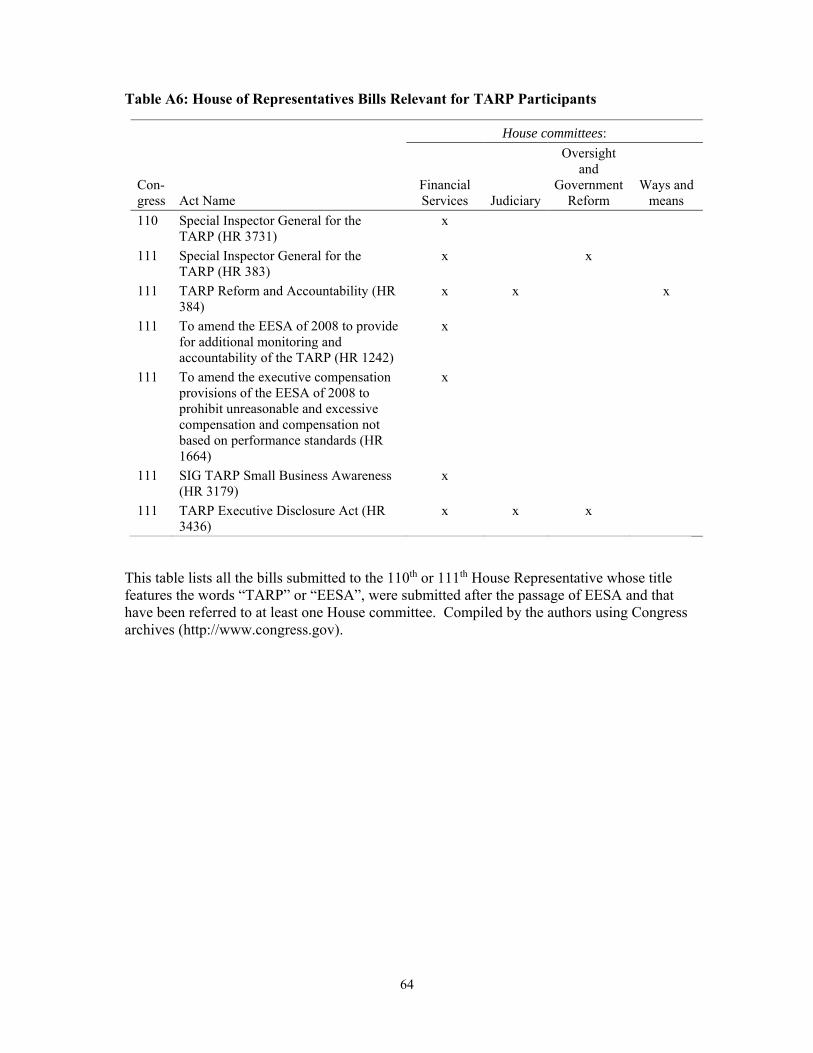
64
Table A6: House of Representatives Bills Relevant for TARP Participants
House committees:
Con-gress Act Name
Financial Services Judiciary
Oversight and
Government Reform
Ways and means
110 Special Inspector General for the TARP (HR 3731)
x
111 Special Inspector General for the TARP (HR 383)
x x
111 TARP Reform and Accountability (HR 384)
x x
x
111 To amend the EESA of 2008 to provide for additional monitoring and accountability of the TARP (HR 1242)
x
111 To amend the executive compensation provisions of the EESA of 2008 to prohibit unreasonable and excessive compensation and compensation not based on performance standards (HR 1664)
x
111 SIG TARP Small Business Awareness (HR 3179)
x
111 TARP Executive Disclosure Act (HR 3436)
x x x
This table lists all the bills submitted to the 110th or 111th House Representative whose title features the words “TARP” or “EESA”, were submitted after the passage of EESA and that have been referred to at least one House committee. Compiled by the authors using Congress archives (http://www.congress.gov).
65
Appendix A4: Aggregate and electoral effects
We have established that TARP recipients increase lending in their home Congress
representative’s district. Our interpretation is that representatives seek to encourage lending
in their district, and TARP recipients respond to local political influences (or the threat
thereof). However, our tests do not show either that aggregate district lending increases, or
that congressional representatives benefit from any higher lending.71 In addition, we have
linked the home-district effect to the characteristics but not the benefits of the incumbent, for
instance in subsequent elections.72
We seek to fill these two gaps simultaneously using a two-stage least squares cross-
sectional regression. The first stage relates aggregate lending growth in a district after TARP
to this district’s total exposure to the home-district effect. Formally, we estimate:
∆ ∙ % ∩ ,
where ∆ is the 2006-2007 to 2008-2009 change in total log mortgage
origination volume in a district (thus including non-frontier areas and all banks). The
explanatory variable of interest % ∩ is the share of mortgages originated by
TARP participants headquartered in the district, measured before the TARP (that is, in 2006-
2007) to avoid reverse causality. This variable captures the prior that districts with a larger
presence of locally headquartered TARP banks stand to gain more from the home-district
effect than other districts.
Stage 2 relates district lending growth to the incumbent’s 2010 electoral performance:
∙ ∆ ,
71 This is because we split lending by counties and banks, and exclude both non-“frontier” areas and large banks. This sharpens identification, but delivers a partial view of total district lending, the likely relevant outcome for the politician. 72 A large theoretical and empirical literature shows that economic conditions influence electoral outcomes, including those of American midterm Congress elections (Lewis-Beck and Stegmaier (2000) and references therein). Most studies concentrate on changes in local income. But Antoniades and Calomiris (2016) show that voters in a county “punish” the incumbent presidential candidate if local credit supply declines, even controlling for county income.
66
where the regressand is Win – 1 if the incumbent wins the 2010 House of Representatives
midterm election, and 0 otherwise, and % ∩ is used as an instrumental
variable for ∆ .73
% ∩ is pre-determined, but still might be correlated with a number
of determinants of lending growth and electoral outcomes; failing to control for these could
lead to a violation of the exclusion restriction. We thus control for characteristics of the
districts’ borrowers, incumbent candidate and electoral competition.74,75 We also include
state fixed effects to control for state-wide shifts in economic conditions or political
preferences. The two equations are estimated on the cross-section of 392 incumbent
congressional representatives who ran for re-election in 2010.76
Table A7 reports the estimation results. Districts more exposed to the home-district
effect experience higher aggregate lending. The coefficients of the first-stage in column 1
indicate that when % ∩ increases by 10%, total post-TARP lending is 4.2%
higher, an economically and statistically significant amount.77 Reassuringly, the second-
stage results show that higher post-TARP lending in the district is associated with a higher
probability that the incumbent wins the 2010 midterm election, when using either total post-
TARP lending growth (column 3) or acceptation rate (column 4) as endogenous variable of
interest. We also find that quantitatively, a one-standard deviation lending increase (+28%,
or $560 million for the average district) is associated with a 10 percentage points higher vote
percentage for the incumbent (results are available upon request). This is a large number; it
73 We estimate a linear probability model despite the dummy regressand due to the presence of fixed effects. 74 We include pre-TARP mean values of all borrower controls included in the main regressions, as well as the post-TARP change in two district-level outcomes available through HMDA – average borrower income and loan size. 75 We include incumbent log number of terms served and party (Republican dummy), and a 2006-2008 representative Republican dummy. Many incumbents are uncontested, and electoral competition might affect politicians’ incentives to cater to constituents’ needs (Levitt and Snyder, 1997). So we control for the 2006 and 2008 winning margin and the 2008 and 2010 log number of candidates. %(TARP ∩ Home)d might affect electoral outcomes through its effect on local labour markets in the banking sector, so we also include the share of employees by the financial industry. Finally, we include the market share of locally headquartered banks to control for the effect of small banks presence on post-crisis lending (DeYoung et al. 2015). 76 We obtain qualitatively similar stage-1 results when using all districts. 77 Alternatively, column 2 shows that the mortgage application acceptation rate rises by a comparably large 0.7 percent.
67
is also close to Levitt and Snyder (1997), who find that $50 million more federal spending in
a district increases incumbent’s performance by 2 percentage points.
In contrast to our main regression results, these tests seek to maximise
representativeness, which comes at the cost of lower precision. While magnitudes should
thus be interpreted with caution, the results qualitatively support the notion that the home-
district effect matters for district lending conditions and political outcomes.
A related question is whether the home-district effect imposes any cost to TARP
participants. Our findings that participants increase lending and application acceptations
conditional on borrower credit risk suggest looser underwriting standards in the home
district.78 To test this we estimate the cross-sectional regression:
∆% ∙ % ,
where ∆% is the change in bank non-performing loan
percentage between the pre-TARP (2006q4-2007q4) and 2010q4, when changes in lending
standards might start appearing on balance sheets. Our explanatory variable of interest is
% , the interaction of a TARP dummy with the bank’s share of home-
district lending before TARP (2006-2007). This captures the notion that participants with a
larger portion of overall lending in their home district are more affected by a relaxation of
home-district underwriting standards compared to other banks.79 The results, reported in
column 5, suggest that a 10% increase in TARP-Home is associated with 0.2 percentage
points higher share of non-performing loan. This effect is quantitatively modest from the
bank’s overall balance sheet point of view, but relatively large compared to the average
change in non-performing loans over the period (+2.8 percentage points).
78 Alternatively, TARP participants might also be able to expand home-district lending by passing on the lower funding costs they might enjoy through TARP (Berger and Roman, 2015) to home-district borrowers. 79 In addition to the components of this interaction, we include the bank and borrower controls used in the main regression (all measured as pre-TARP mean), as well as state fixed effects.
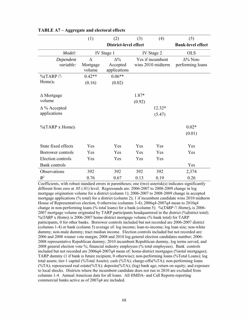
68
TABLE A7 – Aggregate and electoral effects
(1) (2) (3) (4) (5) District-level effect Bank-level effect
Model: IV Stage 1 IV Stage 2 OLS
Dependent variable:
Δ Mortgage volume
Δ% Accepted
applications
Yes if incumbent wins 2010 midterm
Δ% Non-performing loans
%(TARP ∩ Home)d
0.42** 0.06** (0.16) (0.02)
Δ Mortgage volume
1.87* (0.92)
Δ % Accepted applications
12.32* (5.47)
%(TARP x Home)i 0.02* (0.01)
State fixed effects Yes Yes Yes Yes Yes Borrower controls Yes Yes Yes Yes Yes Election controls Yes Yes Yes Yes Bank controls Yes
Observations 392 392 392 392 2,374
R2 0.76 0.67 0.13 0.19 0.26 Coefficients, with robust standard errors in parentheses; one (two) asterisk(s) indicates significantly different from zero at .05 (.01) level. Regressands are: 2006-2007 to 2008-2009 change in log mortgage origination volume for a district (column 1); 2006-2007 to 2008-2009 change in accepted mortgage applications (% total) for a district (column 2); 1 if incumbent candidate wins 2010 midterm House of Representatives election, 0 otherwise (columns 3-4); 2006q4-2007q4 mean to 2010q4 change in non-performing loans (% total loans) for a bank (column 5). %(TARP ∩ Home)d is 2006-2007 mortgage volume originated by TARP participants headquartered in the district (%district total). %(TARP x Home)i is 2006-2007 home-district mortgage volume (% bank total) for TARP participants, 0 for other banks. Borrower controls included but not recorded are 2006-2007 district (columns 1-4) or bank (column 5) average of: log income; loan-to-income; log loan size; non-white dummy; non-male dummy; tract median income. Election controls included but not recorded are: 2006 and 2008 winner vote margin; 2008 and 2010 log general election candidates number; 2006-2008 representative Republican dummy; 2010 incumbent Republican dummy, log terms served, and 2008 general election vote %; financial industry employees (% total employees). Bank controls included but not recorded are 2006q4-2007q4 mean of: home-district mortgages (%total mortgages); TARP dummy (1 if bank is future recipient, 0 otherwise); non-performing loans (%Total Loans); log total assets; tier-1 capital (%Total Assets); cash (%TA); charge-offs(%TA); non-performing loans (%TA); repossessed real estate(%TA); deposits(%TA); (log) bank age; return on equity; and exposure to local shocks. Districts where the incumbent candidate does not run in 2010 are excluded from columns 1-4. Annual American data for all loans. All HMDA- and Call Reports-reporting commercial banks active as of 2007q4 are included.