Political Blockades and Election Timing ∗†

Felix Bierbrauer

MPI, Bonn

Lydia Mechtenberg

WZB, Berlin

September 3, 2010

Abstract

We provide a welfare analysis of early elections in a dynamic model of political competi-

tion with endogenous political blockades. Blockades arise if a party wins an election due to

the support of voters with extreme policy preferences. We show that flexible election timing

has the advantage that political blockades are overcome and political decisions are taken more

frequently, but also the disadvantage that these decisions are of a lower quality. We argue that

the disadvantage of early elections is likely to dominate, but that time-consistency problems

make a constitutional ban on early elections difficult to maintain in a parliamentary democracy.

Keywords: early elections, political blockades

JEL: D72, D61, D82

∗We benefited from comments by Dorothea Kuebler, Christoph Engel, Martin Hellwig, Michael Kurschilgen,

Stephan Tontrup, Philipp Weinschenk, Max Wolf, and Elmar Wolfstetter. We are grateful to participants of seminars

at the Humboldt University, Berlin, the LMU, Munich, of the 2009 Silvaplana Workshop on Political Economy, and

of the 2010 Workshop on Political Economy in Stony Brook.†This research was supported by the Deutsche Forschungsgemeinschaft through the SFB 649 ”Economic Risk”.

1 Introduction

Is a political constitution that allows for snap elections in the interest of the voters? This question

arises due to the diversity of existing constitutional rules of election timing. Although the timing of

general elections is flexible throughout a large part of the democratic world, there are democratic

countries, most prominently the U.S., where it is not. Thus, it is natural to ask “who gets it right”

from the voters’ perspective.

We analyze this question in a dynamic setting in which a left-wing and a right-wing party are

repeatedly competing with each other. Prior to an election both parties nominate candidates. If a

party wins, its candidate becomes the prime minister and the party becomes the ruling party. The

prime minister’s role is to make policy proposals. However, to be implemented a proposal needs

the ruling party’s consent. A driving force in our model is that a prime minister will be reelected

only if he is able to prove his competence. The party, by contrast, has an incentive not to approve

policies that are unattractive to its most loyal voters. This difference in the party’s and the prime

minister’s reputation concerns may give rise to conflicts about the right policy: The prime minister

may be eager to have a political success, e.g. a reduction of unemployment rates, that signals

his competence, even if this requires policy measures that do not conform to the party ideology.

For instance, suppose that a reduction of unemployment rates necessitates a cut of unemployment

benefits. If the left party is ruling, it may not be willing to approve such a policy because this

comes at the cost of losing support among its most loyal voters, who oppose a cut of unemployment

benefits, and therefore weaken its position in future races against the other party. Thus, the party

may be willing to to block the prime minister’s policy proposals.

The contribution of this paper is first to develop a model in which such blockades are an equilib-

rium phenomenon. Second, we analyze how a system with fixed and a system with flexible election

timing cope with political blockades. In particular, we are interested in the question whether po-

litical blockades can be more easily overcome in a system where an early election can be called

whenever a political blockade materializes. We are also analyzing whether voter welfare is higher

in a political system with fixed election timing or in a system with flexible election timing.

Our model builds on different branches of the political-economy literature. The first branch studies

the effects of reputation or career concerns on political and economic outcomes.1 In our paper,

reputation concerns are important for the emergence of political blockades which, in their turn, are

a major reason - and justification - for snap elections.

We model political competition as an infinitely repeated game between a left-wing and a right-

wing party and the voters. This relates our paper to recent work on dynamic models of political

decision-making.2 Our contribution to this line of research is to provide a dynamic model of

endogeneous parliamentary blockades. Moreover, our comparison of political equilibria under fixed

and flexible election-timing relates our work to the literature on the effects that electoral rules and

1The literature on reputation or career concerns dates back to the seminal work of Holmstrom (1999) and De-

watripont, Jewitt and Tirole (1999a, 1999b). Reputation concerns within a dynamic political economy setting have

been studied recently by Fu and Li (2010).2Main contributions are, for instance, Acemoglu et al. (2008), Battaglini and Coate (2008a, 2008b), Fahri and

Werning (2008), Battaglini et al. (2010), and Battaglini (2010).

1

forms of government have on economic outcomes.3 To our knowledge, our paper is the first to

merge these branches of the literature and to analyze effects and determinants of constitutions in

a dynamic setting with reputation concerns.4

Finally, our paper is related to the literature on the strategic termination of governments; see,

for instance, Diermeier and Merlo (2000) and Keppo et al. (2008). 5 However, we differ from this

literature in that we provide a fully microfounded analysis of election timing.6 Moreover, we are

the first to take into account that early elections can serve two very distinct goals: First, they can

be the result of strategic election timing of the government, e.g., a government may want to date

elections prior to the revelation of unfavorable information on its past performance. An empirical

example is Margaret Thatcher who was accused of “cutting and running”, i.e. of strategic election

timing, when she called an election in 1983, shortly before the inflation rate went up, and thereby

capitalized on high polls in the nick of time. Strategic election-timing in that sense is typically

detrimental to voters since it leaves them with less information than optimal about the incumbent.

Second, however, early elections can be the means of overcoming a blockade in parliament and

carry through an agenda that is favored both by the government and the voters. In such cases, early

elections are clearly in the voters’ interest, too. In Germany 2005, chancellor Gerhard Schroder

called an early election. He argued that “ without a new mandate my political programme cannot

be carried forward” (The Independent, 2 July 2005). The German president, whose consent was

needed for an early election to take place, emphasized the country’s exigent need of a strong gov-

ernment capable of enforcing needful though controversial reforms.7

Our formal analysis is based on a model with two infinitely lived parties, called L and R, who

are repeatedly competing with each other. Parties nominate candidates for elections. The winning

party’s candidate, henceforth called the prime minister, makes policy proposals, which need the

approval of the ruling party to pass parliament. The prime minister is office-motivated, and, due

to term limits, can be in office for at most two legislative periods.8

We assume that a prime minister may be competent or incompetent in the sense that she is

3See Persson and Tabellini (2000,2003) for an overview.4Battaglini (2010) is one of the few studies of constitutional rules in a dynamic setting.5This literature treats the behavior of voters as exogenous. Diermeier and Merlo (2000) extend the legislative

bargaining model due to Baron and Fehrejohn (1989) so as to allow for an early dissolution of government. The events

that may trigger dissolutions are exogenous policy and public opinion shocks. Keppo et al. (2008) model election

timing as a response of politicians to an exogenous stochastic process which governs the popularity of different parties.

Earlier contributions to this literature include Balke (1990) and Lupia and Strom (1995). Some of the literature on

political business cycles has also considered flexible election terms, see Chapell and Peel (1979), Lachler (1982), and

Kayser (2005).6Alaistar Smith (1996, 2004), who has greatly inspired our work, has provided a game-theoretic perspective on

election timing. He has analyzed early elections as a signalling game, but in a static setting and without modelling

parliamentary blockades.7Similarly, Japan’s prime minister in 2005, Jun’ichiro Koizumi, justified calling an early election with the purpose

of pursuing a controversial reform (the privatization of the national post) against the opposition in the parliament.8This assumption simplifies the analysis. An alternative interpretation would be that there is a ”natural” limit

to the time any prime minister can stay in office, e.g. because of age. For our results, it is not important why such

a limit exists or how many periods a prime minister can stay in office, as long as the limit is the same for all prime

ministers.

2

- or is not - able to identify effective policies. To illustrate this, suppose that the reduction of

unemployment rates is the most urgent political problem and that there are two types of policy

measures that can be used. On the one hand, Keynesian policies would stimulate macroeconomic

activity. One the other hand, one could also choose a policy that improves individual incentives to

seek for employment, e.g., a reduction of unemployment benefits. Suppose that, depending on cur-

rent economic conditions, only one of these policy measures can effectively reduce unemployment.

We say that a prime minister is competent if she understands what the effective policy measure is,

and is incompetent otherwise.

While in her first term, a competent prime minister seeks to prove her competence to voters, so

as to make sure that she is renominated by her party, and reelected by the voters. However, there

may be a blockade so that the policy that would have to be chosen for that purpose is not accepted

by the ruling party. For instance, blockades arise in our model when (i) the competent policy is

a leftist policy, (ii) the rightist party is ruling, and (iii) the prime minister’s position is weak.9

An empirical example would be a socialist government that has to cut unemployment benefits to

reduce unemployment effectively, but does not find sufficient support for this policy among the

members of the socialist party.10

If early elections are not an option, then it is easy to see that a prime minister who is competent

but blocked is empirically indistinguishable from a prime minister who is incompetent (and may

argue that she is blocked). In both cases, voters just observe that unemployment remained high and

therefore have less confidence in the prime minister’s competence. This implies that the incumbent

party prefers to nominate a newcomer prior to the next election. Consequently, only a competent

prime minister who does not face a blockade can survive in office for two consecutive terms.

If, by contrast, early elections are possible, then a competent prime minister who is blocked

may have an incentive to use them in order to avoid being replaced at the date of the next regular

election. Whether this incentive exists depends on the voters’ beliefs, i.e., on whether voters believe

the prime minister to be likely enough to reduce unemployment, once her majority in parliament

will have become larger. Put differently, the prime minister can use an early election to gain

additional time in office if and only if voters are sufficiently confident that she is competent.

Given such beliefs, however, early elections are attractive for any prime minister, competent or

not, who is unable, for whatever reason, to reduce unemployment prior to the next regular election.

Moreover, early elections are more often attractive for an incompetent prime minister than for a

competent one. This is because a competent prime minister, as opposed to an incompetent one, can

sometimes reduce unemployment, namely whenever there is no blockade, i.e. the effective policy

is supported by the ruling party. Thus, a competent prime minister need not always fear to be

replaced after her first term. Thus, the rational voter believes that a prime minister who calls an

early election is much more likely to be incompetent than competent. Consequently, only if the

9In our model, a prime minister is strong if it was a clear competence advantage relative to the challenger that

made her win elections, implying that she gained all voters in a neighborhood of the median voter. By contrast, her

position is weak if she just won by chance.10Thus, our model shows that while only Nixon could go to China, a prime minister in a parliamentary system

could probably not do the same. Whenever a prime minister has to rely on his party that, in its turn, has to secure

the support of voters with extreme policy preferences, the prime minister better toes the line if she wants to stay in

office.

3

opposition’s candidate makes an even worse impression will the voter reelect the prime minister at

an early election.

There are two conclusions from these considerations. First, voters cannot discern whether the

motives behind a given snap election are legitimate or not. The reason is that an incompetent

prime minister can always blame the need to compromise with her party for her lack of success.

Second, an early election confronts the voter with the choice between a prime minister who is

unlikely to be competent and an alternative candidate who is even worse. This follows because the

incumbent prime minister calls an early election only if she is sufficiently likely to win. But this

requires that the opposition’s candidate must appear even less appealing to the voters.11 Thus,

whereas a constitution that bans early elections leads to too frequent replacements of competent

prime ministers, a constitution that allows for early elections does exactly the reverse: It leads to

too frequent reelections of incompetent prime ministers. Incompetent prime ministers are mostly

reelected in early elections after a parliamentary blockade that would not have occurred were early

elections banned constitutionally.

However, this downside of early elections is potentially counterbalanced by the fact that early

elections affect the timing of political decisions in a way that favors fast decision-making. We assume

that the major political initiatives of a government are undertaken shortly after an election. This

assumption is meant to capture a stylized fact: In parliamentary democracies, political activity

declines as the end of the legislative period approaches.12

Consequently, an early election implies that the next substantial political decision is taken

earlier. In our example, given that unemployment will not go down prior to the next regular

election, an early election offers the chance that the effective policy against unemployment can be

implemented immediately, rather than after the next regular election.

These considerations show that the answer to the question whether a political constitution

should include the possibility to call for an early election depends on the assessment of a quality-

quantity-tradeoff. On the one hand, it is more likely that an early election prolongs the career of

an incompetent prime minister. This gives rise to a negative quality effect. On the other hand, the

expected time distance between two consecutive political decisions is lower in a system in which

early elections occur frequently. Thus, over time, important political decisions are taken more

frequently in such a system.

The remainder of this paper is organized as follows. In Sections 2, we introduce an illustrative

model of political blockades that we extend by early elections in Section 3. In the illustrative

model, we treat bargaining in parliament as a black box. We use the illustrative model to show

the main trade-off between banning early elections, with the consequence of having more blockades

of “good” agendas, and allowing for early elections, with the consequences of more “bad” agendas

being carried through. In Section 4, we study our main model with endogeneous parliamentary

11A possible reason is that the opposition party is surprised enough by the timing of the election to be unable to

produce a suitable candidate. See Smith (2004) for empirical evidence on this.12This happens for a variety of reasons. Politicians start to prepare themselves for the upcoming election, the

current leaders potentially suffer from a lame-duck effect, or the current government seeks to avoid controversies as

the next election comes closer. Empirically, the decline of important political decisions over a legislative term has

been documented by Martin (2004).

4

blockades, heterogeneous voters and uncertainty about the outcome of early elections. Our anal-

ysis of the main model provides a microfoundation for political blockades and a welfare analysis

of early elections. Moreover, Section 4 presents our insights regarding the distributional effects

of constitutionally allowing for early elections and argues that a “stable” constitution allows for

early elections although this does not maximize voters’ welfare under plausible conditions. The last

section contains a discussion of our results. All proofs are in the Appendix.

2 An illustrative model of political blockades

Consider a country with a large number of homogeneous citizens who are infinitely lived. Periods are

denoted by T ∈ {0, 1, 2, 3, ...}. Citizens are born in T = 0 either as politicians who can implement

policies or as voters who are affected by policies, so that there is a large number of both types.

Their common discount factor is δ. We first consider a model in which the timing of elections is

inflexible, and political decisions are taken at specific dates. Specifically, we assume that in each

second period T ∈ {1, 3, 5, ...}, an election is held and a political decision pT ∈ [−2, 2] is taken. If

pT ∈ [−2, 0], the implemented policy is leftist ; otherwise, it is rightist.

2.1 Parties

We assume that any politician is born in T = 0 as a member of one of two parties, L or R, and

that elections are always between a politician from L, and a politician from R.

Parties must nominate candidates before elections. Due to term limits, a party can nominate

only members that have not been elected more than once in the past. Moreover, we assume that

former prime ministers that have been voted out of office are not available as candidates any more.

If the incumbent prime minister has not yet been reelected, the ruling party has to decide whether

to nominate her again, or to draw another party member randomly instead. If the incumbent prime

minister has been relected already, the ruling party must randomly draw a new candidate. The

opposition party must always randomly draw a candidate before elections. Hereafter, we refer to

randomly drawn candidates as newcomers.

Parties are office-motivated. The per-period utility of party J , J ∈ {L,R}, amounts to

vT,J =

{1, if J is ruling in T ,

0, otherwise.

Thus, when deciding whether to renominate the incumbent prime minister after her first leg-

islative period, the ruling party chooses j ∈ { incumbent, newcomer} in order to maximize the

expected present value of vT,J , with expectations taken over all future uncertain events.

2.2 Elections

To have a policy pT implemented, one of the two candidates must be elected at the beginning of

that period. We refer to an elected politician as the prime minister. A legislative period has the

length 2.

5

The maximum period that a prime minister can stay in office comprises two legislative periods,

i.e. any politician can be reelected at most once.13 A policy pT is only implemented in the first

half of the legislative period.

The decision about a policy pT is made jointly by the prime minister and the parliament. The

joint decision-making is presented in a reduced form below and as a fully microfounded interaction

in section 4 where we present the main model.

2.3 Voters’ utility

A policy pT affects utilities of voters uT . The way in which voters’ utilities are affected depends

on the state of the economy ωT , a random variable that is uniformly distributed over [−1, 1]. The

random variables ωT and ωT ′ , for T ′ 6= T , are assumed to be stochastically independent.

A voter’s utility from a political decision taken in period T is given by

uT = −λ (pT , ωT ) =

{0, if pT = ωT ,

−1, otherwise.

In even periods, i.e., when no policy is implemented, voters have a default utility: uT = 0.14

2.4 Voting

At election date T , voters vote sincerely, in a forward looking way, i.e., at date T , a person votes

for party L only if the expected present value of his utility is larger if party L wins, and votes for

party R otherwise. If indifferent, the voter flips a coin.

2.5 Types of politicians

We assume that prime ministers are not necessarily competent to implement the efficient policy

p∗T = ωT . Thus, we distinguish between competent and incompetent types of politicians. If a

competent politician becomes prime minister she observes ωT , and remains uninformed otherwise.

An incompetent politician does not learn ωT . The prior probability that a politician is competent

is assumed to be equal to 12 . Neither politicians who are not in office nor voters can observe ωT .

Moreover, politicians are purely office-motivated, like their parties: When they have been drawn

to be a candidate for elections, their per-period-utility amounts to 1 if they are in office and to 0

otherwise.

2.6 Policy implementation

A policy pT is implemented as follows: The prime minister makes a proposal pT that is implemented

if and only if it is accepted in parliament. Otherwise, a status-quo policy pT = 0 is implemented.

In the given setup, we model the interaction between the prime minister and the ruling party in

reduced form.

13The assumption that there is some upper bound on reelections is important for our results, but nothing hinges

on its being equal to one.14The utility levels 0 and −1 are based on normalizations that do not carry further meaning. In the main model

in Section 4, we provide a richer description of preferences.

6

In the main model in Section 4, we provide a rigorous microfoundation of the reduced form

below. For now, parliament is viewed as a device D that is programmed so that it always approves

the policy proposals of a “strong” prime minister, but approves those of a “weak” prime minister

only if they conform with party ideology. More specifically, we make the following assumptions:

Assumption 1 In periods T ∈ {1, 3, 5, ...}, the prime minister from party J ∈ {L,R} sends a

private policy suggestion pT ∈ [−2, 2] to a device D. D is programmed as follows: If the prime

minister has already been reelected once, it implements pT . If the prime minister has not been

reelected yet, but has won her first election against the former incumbent, D also implements pT .

If the prime minister has not yet been reelected and has won her first election against another

newcomer, the following holds true: If J = L, D implements pT = pT if pT ∈ [−2, 0] and pT = 0

otherwise. If J = R, D implements pT = pT if pT ∈ [0, 2] and pT = 0 otherwise.

The interpretation is as follows: A prime minister who has already been confirmed in office twice

has a stronger position in parliament than a prime minister who has been confirmed in office only

once. Also, a prime minister who, as a newcomer, has won her first election against the experienced

incumbent has a stronger position in parliament than a prime minister who has won only against

another newcomer.

With a strong position in parliament, a prime minister from party L (R) can implement both

left-wing and right-wing policies, i.e., policies in the left and right half of the interval [−2, 2].

With a weak position in parliament, the prime minister from party L (R) can only implement left-

wing (right-wing) policies, i.e., policies in the interval [−2, 0] ([0, 2]). The strength of position in

parliament and the differences in implementable policies between strong and weak prime ministers

will be endogenized as equilibrium outcomes in section 4.15

We assume that the prime minister’s policy suggestion pT is not publicly observable. This

assumption takes to the extreme the fact that not all bargaining procedures within the government

can be observed by the public. Voters update their beliefs about the prime minister’s type after

having observed the implemented policy pT and after having realized uT . We may therefore assume,

without further loss of generality, that a prime minister chooses proposals subject to the constraint

that they will be implemented by D.16

As a tie-breaking rule, we therefore impose the following assumption.

Assumption 2 If a prime minister is indifferent between various proposals that have the same

implications for her chance of winning a future election, she will choose one that maximizes voter

utility subject to being implemented by D.

15In Section 4, we make our distinction between “weak” and “strong” prime minister more substantive. In the

main model, a “strong” prime minister has won a large majority in the election, whereas a “weak” prime minister

has won only a small majority. Moreover, a weak prime minister is dependent on the support of “extremist” voters.16That being said, if instead we assumed that policy proposals were observable, the analysis below would remain

unaffected, except that our proofs would involve one additional step, namely to show that, in equilibrium, voters are

unable to distinguish proposals made by competent prime ministers who cannot implement pT = ωT from proposals

made by incompetent ones.

7

2.7 The game

In sum, the game is as follows:

1. Nature draws types in T = 0: There is a large number of voters, and there is also a large

number of politicians, half of whom would be competent prime ministers and half of whom

would be incompetent. A politician’s type is her private knowledge. Nature randomly sorts

politicians into parties L and R and programs the device D.

2. Parties nominate their candidates at the end of periods T ∈ {0, 2, 4, ...}. (A candidate can

run in at most two consecutive elections.) If a party cannot or does not want to renominate

an incumbent, it randomly draws a newcomer from among its members. Elections are held

at T ∈ {1, 3, 5, ...}. Voters vote sincerely and flip a coin if indifferent. A simple majority rule

determines the winner.

3. The state of the economy, ωT , is drawn at the beginning of each time period. It is observed

by the prime minister if and only if she is competent.

4. In odd periods, the prime minister sends a private policy suggestion pT to the device D. D

implements the policy pT according to Assumption 1. Voters observe pT , receive their payoffs

and update their beliefs about the prime minister’s type.

5. At the end of periods T + 1 ∈ {2, 4, 6...}, parties nominate candidates for next elections. In

T + 2 ∈ {3, 5, 7, ...}, elections are held again.

2.8 Equilibrium analysis

We now turn to the analysis of the equilibria of the game. The solution concept is Refined Per-

fect Bayesian Equilibrium which requires that the strategies of the voters, parties, and the prime

minister are mutually best responses for given beliefs about the prime minister’s type and that be-

liefs are derived from Bayes’ rule whenever possible. The refinement is a condition of stationarity:

Strategies of all players are the same in two continuation games that start with two newcomers

competing during (early or regular) elections.17

Proposition 1 There is a stationary perfect Bayesian equilibrium with the following properties:

• Policy Outcomes: If the prime minister is incompetent, then the outcome of her policy is

uT = −1. If the prime minister is competent, the two events uT = 0 and uT = −1 have equal

probability in her first legislative period, and uT = 0 in her second legislative period.

• Nomination decisions: The ruling party in T nominates the prime minister for elections in

T + 2 only if uT = 0, provided that the prime minister has not been reelected already. In all

other cases, the party nominates a newcomer.

17Note that we do not restrict the analysis to Markov equilibria. This is because equilibria of the main model

that will be presented in section 4 include trigger strategies. We will omit time indices when this does not create

confusion.

8

• Election Outcomes: The prime minister runs for a second term only if she has proven to

be competent, uT = 0. In this case her party wins with certainty. Otherwise, both parties

nominate a newcomer, and each of them wins with probability 12 .

Proposition 1 is our benchmark case of a political equilibrium with blockades. Its main feature

is that a prime minister needs to prove her competence (by means of generating the good outcome

u = 0) in order to be reelected. Moreover, there are situations in which a competent prime minister

is blocked in the following sense: the policy choice that would reveal her competence is not approved

by parliament (i.e., by D). Consequently, a blocked competent prime minister and an incompetent

one are empirically indistinguishable from the perspective of voters. Conditional on u = −1, the

probability that the prime minister is competent equals

Pr(u = −1 | comp.) Pr(comp.)

Pr(u = −1 | comp.) Pr(comp.) + Pr(incomp.)=

1

3, (1)

which is less than 12 , i.e., less than the probability that a newcomer would be competent. Hence,

after having realized a utility of −1, voters prefer a newcomer over the incumbent, which implies

that the incumbent who has produced the bad outcome −1 will not be nominated a second time

by her party. Thus, both incompetent and competent but blocked prime ministers are replaced at

the end of their first term in office.

3 Early elections in the illustrative model

We now extend the model of the previous section and assume that a prime minister who has been

elected in period T has the option to call for an early election in T + 1, rather than waiting for the

next regular election in period T + 2. If an early election takes place, they do so after the utility

uT from the prime minister’s first policy measure is realized. In an early election, the incumbent

runs against a newcomer.

An early election affects the timing of political decision making. A prime minister’s call for

early elections makes her second legislative period start earlier if she becomes reelected. Since the

device D is programmed such that it implements any policy suggestion of the prime minister once

she has been confirmed in office twice, this means that early elections indeed make it possible to

overcome a parliamentary blockade.

We impose one additional assumption to ensure that a prime minister who faces a blockade

indeed has, at least occasionally, an incentive to call an early election: With positive probability,

the opposition party “looks bad” in the middle of the term, so that the incumbent can foresee that

she herself will win the early election.18

To capture this formally, the model is extended as follows: In T = 0, nature sorts the politicians

in either party in two pools, labeled 1 and 2, respectively. A politician in pool 1 is competent with

probability 12 , while a politician in pool 2 is competent with probability k < 1

2 . When nominating

candidates, parties have access to only one of their two pools. The ruling party has always access

18The empirical interpretation would be that an incumbent’s decision whether or not to call an early election is

based on publicly available poll data that document the current standing of the opposition party.

9

to pool 1. However, with probability ρ = 12 , nature, directly after elections, shuts down pool 1

of the opposition party for one time period, opening pool 2 instead. Thus, only if the upcoming

election is a regular election as opposed to an early election, pool 1 is open for both parties with

certainty; and a newcomer running in a regular election is competent with probability 12 as in the

illustrative model. However, if the upcoming election is an early election, then it can happen that

only the ruling party has access to its pool 1. Whether or not pool 1 is open for the opposition

party is publicly observable. This creates an incentive for the ruling party to have early elections in

order to get the opposition party at a disadvantage. For computational ease, we assume hereafter

that k = 16 .19

This modelling choice is meant to capture an important difference between early and regular

elections. Early elections, or snap elections, often come as a surprise, therefore being likely to bring

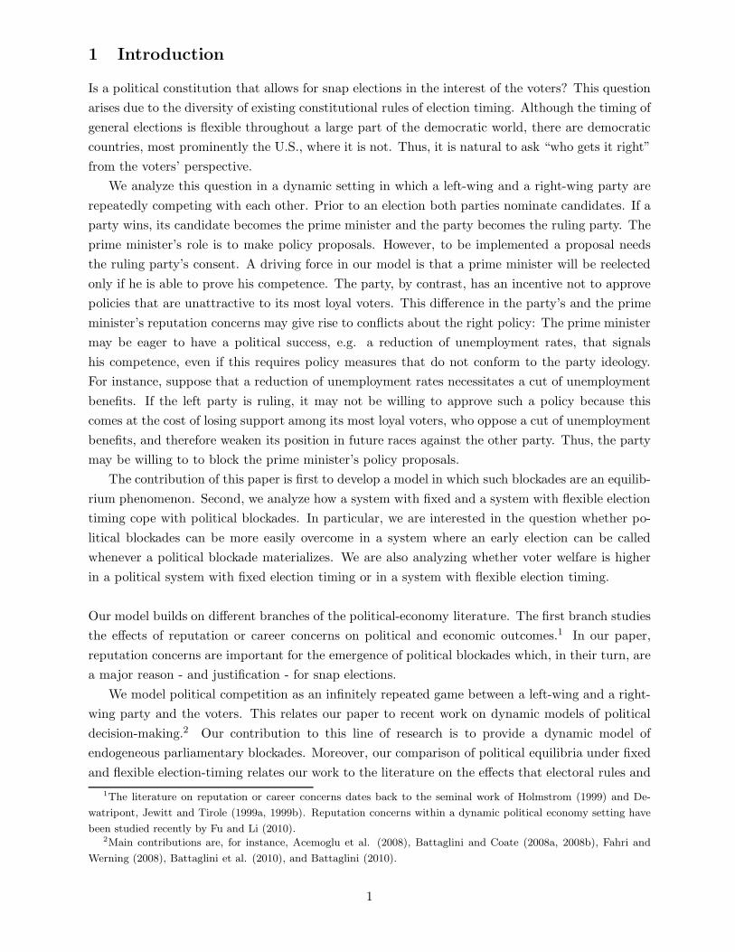
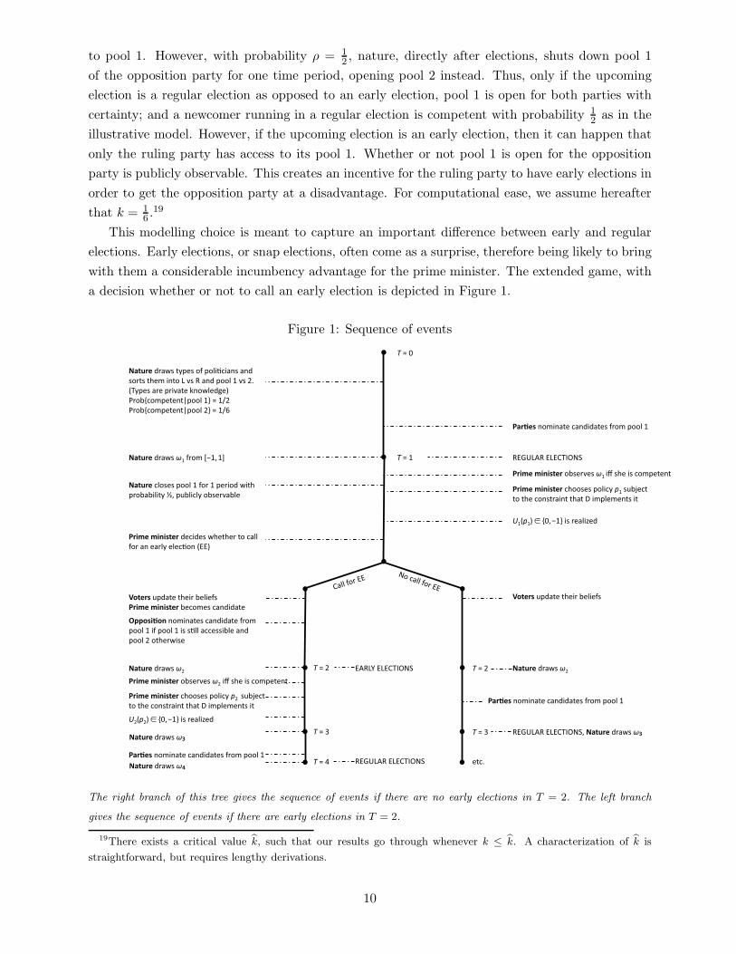
with them a considerable incumbency advantage for the prime minister. The extended game, with

a decision whether or not to call an early election is depicted in Figure 1.

Figure 1: Sequence of events

The right branch of this tree gives the sequence of events if there are no early elections in T = 2. The left branch

gives the sequence of events if there are early elections in T = 2.

19There exists a critical value k, such that our results go through whenever k ≤ k. A characterization of k is

straightforward, but requires lengthy derivations.

10

3.1 Equilibrium analysis

We have seen that without early elections, any prime minister, competent or not, who is unable to

deliver the good outcome u = 0 in her first term, will be replaced by a newcomer in the subsequent

election. The following Proposition establishes that an incumbent prime minister will use an early

election to avoid replacement whenever the opposition party is weak.

Proposition 2 There exists a cutoff-value δ, so that for all δ ≤ δ, there is a stationary perfect

Bayesian equilibrium with the following properties:

1. Policy outcomes, nomination decisions prior to regular elections, and the outcomes of regular

elections are as described in Proposition 1.

2. Early elections take place in T + 1 if and only if the preceding history is as follows: In period

T there is a regular election that is won by a newcomer and the policy outcome is uT = −1.

At date T + 1, the opposition party’s candidate has to be drawn from pool 2.

This equilibrium is such that both an incompetent prime minister and a competent prime

minister who cannot implement p = ω initiate early elections if the opposition party is weak. More

precisely, both of them call for early elections if the opposition party must draw her candidate

for early elections from the inferior pool 2. Both of them can thereby avoid being replaced by a

newcomer in T + 2, gaining additional time in office until T + 3.

This works because, if early elections are initiated, voters infer that the prime minister is either

incompetent or that D did not implement p = ω. Consequently, they, once more, believe the prime

minister to be competent with posterior probability of 13 . (The reasoning is the same as the one

that led to equation (1) above.) This probability, however, is larger than 16 , i.e., larger than the

opposition’s candidate’s probability of being competent. Consequently, voters reelect the prime

minister.

The existence of the equilibrium in Proposition 2 requires that the discount factor δ does not

exceed a threshold level δ. This is due to the fact that in an early election the prime minister

can run for only one additional legislative period, and the newcomer can run for two legislative

periods. Hence, if both candidates were equally likely to be competent, the newcomer would be

more attractive for the voters because, in case of being competent, the latter can deliver the good

outcome p = ω twice. If δ is low enough, then the prime minister’s competence advantage dominates

this effect so that she wins in an early election.

There are other stationary perfect Bayesian equilibria than the one described in Proposition 2.

In particular, the equilibrium without early elections that has been characterized in Proposition

1 survives the extension of the model. This equilibrium can be sustained by off-the-equilibrium

beliefs such that, whenever the incumbent calls for an early elections, voters believe her to be

incompetent with probability 1.

More importantly, however, there is no equilibrium that has political blockades and in which the

use that is made of early elections distinguishes an incompetent prime minister from a competent

one who cannot implement p = ω. Formally, there is no equilibrium that is fully separating,

11

in the sense that the action “early election” is chosen only by a competent or an incompetent

type. Suppose, for instance, that only competent prime ministers call for early elections. In such

an equilibrium, conditional on an early election taking place, voters would know that the prime

minister is competent and reelect her. But then the incompetent type would have an incentive to

mimic the competent type and also initiate an early election. Otherwise her incompetence would

be revealed prior to the next regular election and she would not get a second nomination. With

similar arguments, one can show that there is no equilibrium in which only an incompetent prime

minister initiates early elections. We summarize this reasoning in the following Proposition, which

we state without proof.

Proposition 3 There is no equilibrium in which early elections occur and in which the decision to

initiate an early election reveals the prime minister’s type.

3.2 A comparison of the two equilibria

We provide a comparison of the equilibrium without early elections in Proposition 1 and the

equilibrium with early elections in Proposition 2 in terms of a quantity and a quality measure.

Let 1NcT be an indicator function that takes the value of 1 if, in the equilibrium without early

elections, the prime minister in period T is competent. We use the expected present value CN =

E[∑

∞

T=1 δT−11NcT ] as a measure of competence in the equilibrium with no early elections, i.e.,

as a quality measure. Also, let 1NpT be an indicator function that takes the value of 1 if, in

the equilibrium without early elections, a political decision is taken in period T . We interpret

PN = E[∑

∞

T=1 δT−11NpT ] as a quantity measure. For the equilibrium with early elections, we define

the measures CE and PE in an analogous way.

Proposition 4 CN > CE and PE > PN .

The proposition establishes that the prime minister is less likely to be competent in a system

with early elections. While early elections make it possible that both a competent prime minister

and an incompetent prime minister gain additional time in office, the Proposition shows that this

effect is more pronounced for the incompetent prime ministers. The reason is that a competent

prime minister will occasionally be able to prove her competence immediately, namely in those

circumstances where D implements her suggestion p = ω. In this case early elections are not

attractive to her because she will win the next regular election with certainty. Hence, a competent

prime minister uses early elections only occasionally, namely if D does not implement p = ω. An

incompetent prime minister, by contrast, always makes use of early elections to avoid being replaced

by a newcomer in the next regular election.

However, in the system with early elections more political decisions are taken. The reason

is that political decisions are always taken immediately after elections are held, and that with

early elections, the average time distance between two consecutive elections is strictly smaller than

without.

12

A welfare analysis of early elections has to compare the importance of the quantity and the

quality effect. In the current setting, with normalizations so that utility equals 0 if there is compe-

tent policy and −1 otherwise, this exercise is not very interesting: Avoiding political decisions is

the dominant concern so that voters would clearly prefer the equilibrium without early elections.

We will therefore come back to this question in the context of the richer model that we introduce

in the next section.

4 The main model with endogeneous parliamentary blockades

We will now introduce two new elements. First, we introduce heterogeneity among voters. This

makes it possible to endogenize the parliamentary blockades that were treated as exogenous in

the previous sections. In particular, we will show that there are voters who benefit from political

blockades and whose support is important for the parties, so that they, occasionally, have an

incentive to block the prime minister’s policy proposals.

Second, we model election campaigns as a source of randomness such that the outcome of an

election is no longer perfectly predictable. For instance, if both parties nominate a newcomer, then

there is a probability that one candidate will outperform the other in the election campaign and win

with certainty. Also, we assume that voters can choose to abstain from an election. As will become

clear, these extensions make our model more realistic in that there are two types of elections. On

the one hand, there are elections where it is important for the parties to get enough support from

the voters with extreme policy preferences. For instance, if the very leftist voters abstained and

the very rightist participated in the election, then party R would win. This creates an incentive

for the left party to fight for the votes of the very left. On the other hand, there are races where

the focus is on the voters in the middle, and the winning party is successful in getting the support

of all voters that are close to the median.

With probabilistic voting outcomes, early elections may be lost by the incumbent. As docu-

mented by Smith (2004), this happens occasionally.

4.1 Heterogeneity of voters

We introduce heterogeneity of voters by assuming that a voter is characterized by a type θ ∈ [−1, 1].

If a political decision in period T is taken, then a voter realizes a utility of

u(p, ω, θ) = gT − λ(p, ω, θ) .

The term gT is a common value component. It is a utility gain that every voter realizes if a

political decision is taken in period T .20 We assume that gT is a random variable with support

[0, g] and expected value ge. Also, the random variables gT and gT ′ , for T ′ 6= T , are assumed to be

stochastically independent.

20In the illustrative model, this term has been normalized to zero.

13

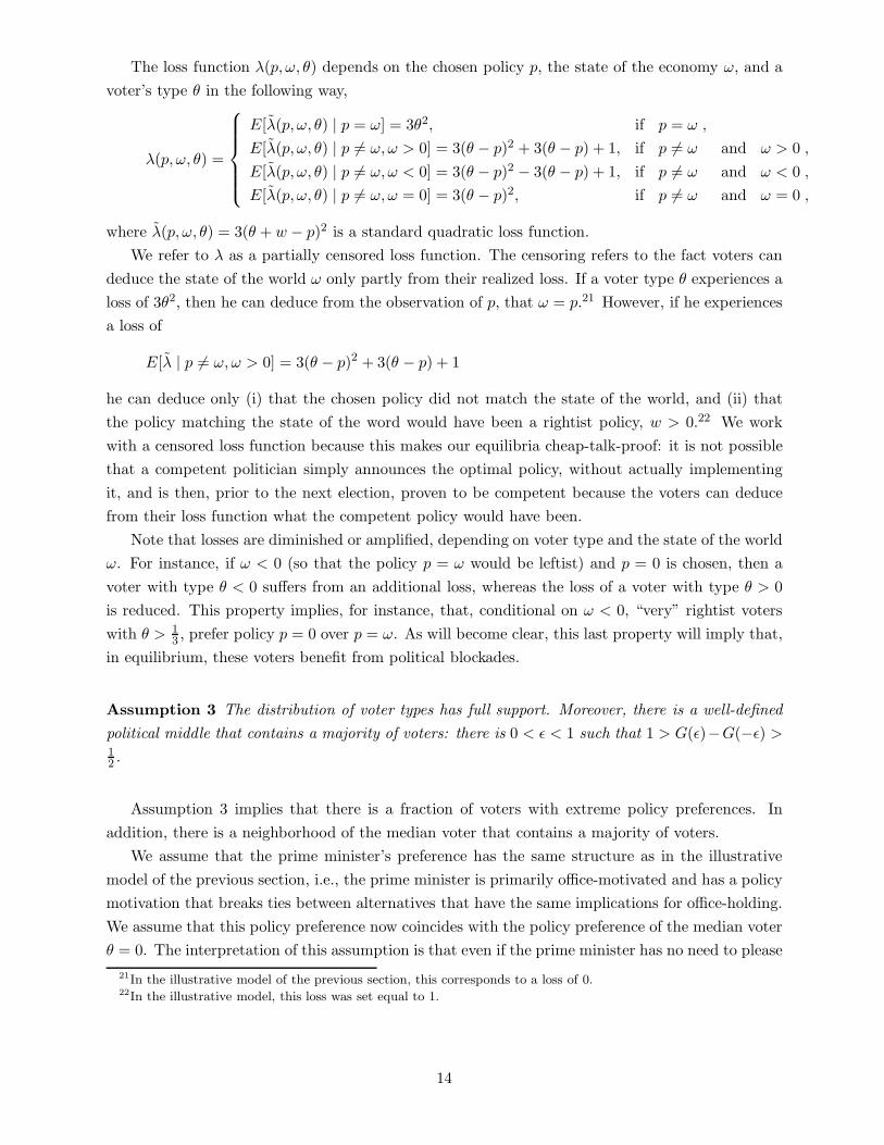
The loss function λ(p, ω, θ) depends on the chosen policy p, the state of the economy ω, and a

voter’s type θ in the following way,

λ(p, ω, θ) =

E[λ(p, ω, θ) | p = ω] = 3θ2, if p = ω ,

E[λ(p, ω, θ) | p 6= ω, ω > 0] = 3(θ − p)2 + 3(θ − p) + 1, if p 6= ω and ω > 0 ,

E[λ(p, ω, θ) | p 6= ω, ω < 0] = 3(θ − p)2 − 3(θ − p) + 1, if p 6= ω and ω < 0 ,

E[λ(p, ω, θ) | p 6= ω, ω = 0] = 3(θ − p)2, if p 6= ω and ω = 0 ,

where λ(p, ω, θ) = 3(θ + w − p)2 is a standard quadratic loss function.

We refer to λ as a partially censored loss function. The censoring refers to the fact voters can

deduce the state of the world ω only partly from their realized loss. If a voter type θ experiences a

loss of 3θ2, then he can deduce from the observation of p, that ω = p.21 However, if he experiences

a loss of

E[λ | p 6= ω, ω > 0] = 3(θ − p)2 + 3(θ − p) + 1

he can deduce only (i) that the chosen policy did not match the state of the world, and (ii) that

the policy matching the state of the word would have been a rightist policy, w > 0.22 We work

with a censored loss function because this makes our equilibria cheap-talk-proof: it is not possible

that a competent politician simply announces the optimal policy, without actually implementing

it, and is then, prior to the next election, proven to be competent because the voters can deduce

from their loss function what the competent policy would have been.

Note that losses are diminished or amplified, depending on voter type and the state of the world

ω. For instance, if ω < 0 (so that the policy p = ω would be leftist) and p = 0 is chosen, then a

voter with type θ < 0 suffers from an additional loss, whereas the loss of a voter with type θ > 0

is reduced. This property implies, for instance, that, conditional on ω < 0, “very” rightist voters

with θ > 13 , prefer policy p = 0 over p = ω. As will become clear, this last property will imply that,

in equilibrium, these voters benefit from political blockades.

Assumption 3 The distribution of voter types has full support. Moreover, there is a well-defined

political middle that contains a majority of voters: there is 0 < ǫ < 1 such that 1 > G(ǫ)−G(−ǫ) >12 .

Assumption 3 implies that there is a fraction of voters with extreme policy preferences. In

addition, there is a neighborhood of the median voter that contains a majority of voters.

We assume that the prime minister’s preference has the same structure as in the illustrative

model of the previous section, i.e., the prime minister is primarily office-motivated and has a policy

motivation that breaks ties between alternatives that have the same implications for office-holding.

We assume that this policy preference now coincides with the policy preference of the median voter

θ = 0. The interpretation of this assumption is that even if the prime minister has no need to please

21In the illustrative model of the previous section, this corresponds to a loss of 0.22In the illustrative model, this loss was set equal to 1.

14

the median voter in order to increase her reelection probability, she behaves “opportunistically” in

the sense of maximizing the support of her policy proposals in the general public.23

4.2 Large and small majorities

In the following, we distinguish between two types of outcomes of an election: We say that a party

gains a large majority if its vote share is strictly larger than 12 . If the vote share is exactly equal

to 12 and the winner of the election is determined by a coin flip, we say that the ruling party’s

majority is small.

In the following we construct equilibria such that the behavior of the ruling party depends on

whether its majority is large or small. In particular if, say, party L rules with a small majority,

then it will block any policy proposals p > 0, i.e., such policy proposals will not pass parliament.

Analogously, if party R rules with a small majority no policy p < 0 will pass parliament. However,

if the ruling party’s majority is large, these constraints are no longer binding.

We will come back to the construction of these equilibria below. For now we want to emphasize

that parliament in these equilibria reproduces the behavior of the exogenous device D that we used

in the previous section as a reduced form model of parliament. If the prime minister has managed

to gain a large majority in an election, this implies that she has a strong position vis-a-vis the

parliament and can implement any policy she likes. Otherwise, her position is weak and she has to

compromise with the ruling party’s ideology.

For the game-theoretic analysis, the distinction between large and small majorities adds the

following complication. Generally, game-theoretic treatments of voting decisions give rise to mul-

tiple equilibria. In elections with only two possible outcomes, e.g., a victory for L versus a victory

for R, only one of those many equilibria survives the elimination of weakly dominated strategies.

In our model, however, a voting decision now has four possible outcomes (a large majority for L,

a small majority for L, a large majority for R or a small majority for R) so that we cannot rely

on the elimination of dominated strategies. We therefore impose the following assumptions on the

voting behavior of individuals.

Assumption 4 If a large majority for one of the parties is strictly preferred by all voters with

types θ ∈ [−ǫ, ǫ], then all of these voters vote for this party.

This assumptions says that if all voters in a neighborhood of the median prefer that one of the

parties wins with a large majority, then these voters manage to coordinate their behavior in such

a way that they indeed induce their preferred outcome.

Assumption 5 Suppose that a voter is indifferent between a large majority for L and a large

majority for R. Then he votes for party L if he prefers a small majority for L over a small

23Given that the median voter’s preferred policy is a unique Condorcet winner, we can define opportunism equiv-

alently as the objective to minimize the number of voters who prefer an alternative policy over the policy proposal

of the prime minister.

15

majority for party R, and votes for party R otherwise. In case of being indifferent, he votes for

each party with probability 12 .

For our equilibrium analysis below, this assumption ensures that the electorate splits at the

median whenever no candidate has a competence advantage after the election campaign. In this

case, all voters to the left of the median vote for L and all voters to the right of the median vote

for R.

4.3 Probabilistic Voting

Prior to any election, there is an election campaign in which one candidate may outperform the

other – in the sense that in the view of the voters she is more likely to be competent – or in which

the two candidates tie. The outcome of the election campaign influences the result of an election

and, in particular, whether the winning party has a large or a small majority.

Formally, we model the outcome of an election campaign as the realization of a random variable

β which takes values in {−1, 0, 1} and is generated as follows: β = αL − αR, where αL and αR are

independent random variables that take the values 0 and 1 with the following probabilities

Pr(αJ = 1 | tj = c) = Pr(αJ = 0 | tJ = i) = η ,

where tJ ∈ {c, i} is the type of party J ’s candidate. We assume that η ∈ (12 , 1), so that a competent

candidate is more likely to get a good signal, αJ = 1, and an incompetent one is more likely to

get a bad signal, αJ = 0. Voters do not observe αL and αR. They only get a signal β of the

relative competence of the candidates. The informational content of β depends on the prior beliefs

of individuals on a candidate’s type. For instance, if two newcomers compete, then both are ex ante

equally likely to be of type c. If voters observe that β = 1, then the conditional probability that

the candidate from party L is competent exceeds the conditional probability that the candidate

from party R is competent. If β = 0, then both are equally likely to be of type c, etc.

4.4 Equilibrium Analysis

The model can be solved analytically.24 However, for ease of exposition, we impose in the following

the assumptions that k = 16 , ge = 3

4 , δ = 12 , and η = 3

4 . This allows us to use numerical methods –

as opposed to lengthy algebraic manipulations of inequalities – in order to illustrate the properties

of the equilibria we are analyzing.

For the same reasons as in the previous section, a constitution that enables a prime minister

to initiate early elections in the middle of a legislative period gives rise to multiple equilibria.

The following Proposition characterizes an equilibrium where early elections never arise. In this

equilibrium, voters would interpret an early election as indicating that the prime minister must be

incompetent so that the prime minister would lose with probability 1.

Proposition 5 Let ge = 34 , δ = 1

2 , and η = 34 . Under Assumptions 3, 4, and 5, there is a

stationary perfect Bayesian equilibrium with the following properties:

24In the Appendix, we explicitly derive all expressions that are relevant for a characterization of equilibrium.

16

• Political Blockades: If Party L (R) has a small majority, it accepts the prime minister’s

policy proposal if and only if p ≤ 0 (p ≥ 0). Otherwise it accepts any policy proposal.

• A prime minister never initiates early elections. Policy Outcomes and Nomination Decisions

are as in Proposition 1. The implemented policy is p = 0 if the prime minister is incompetent

or blocked, and p = ω, otherwise.

• Elections: The prime minister runs for a second term only if she has implemented p∗ = ω.

In this case her party wins with a large majority. If both parties nominate a newcomer, then

the outcome is as follows: If β = 0, there is a small majority for L or a small majority for

R, with equal probability. If β = 1, party L wins with a large majority ; and if β = −1, party

R wins with a large majority.

Proposition 5 establishes that political blockades are part of an equilibrium with heterogeneous

voters. Otherwise, it establishes the same results as Proposition 1, except that there is a richer set

of election outcomes: An election where both parties nominate a newcomer does not necessarily

lead to a small majority for the winning party. If one candidate appears superior in the election

campaign, her party will win with a large majority.

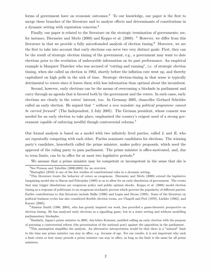
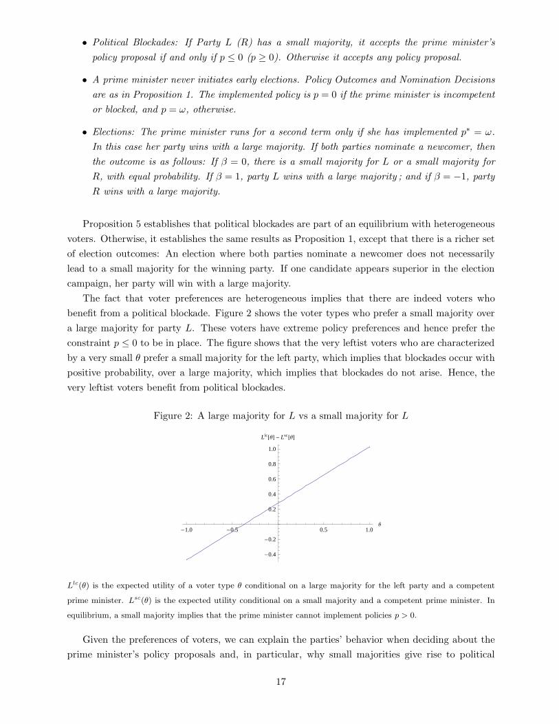
The fact that voter preferences are heterogeneous implies that there are indeed voters who

benefit from a political blockade. Figure 2 shows the voter types who prefer a small majority over

a large majority for party L. These voters have extreme policy preferences and hence prefer the

constraint p ≤ 0 to be in place. The figure shows that the very leftist voters who are characterized

by a very small θ prefer a small majority for the left party, which implies that blockades occur with

positive probability, over a large majority, which implies that blockades do not arise. Hence, the

very leftist voters benefit from political blockades.

Figure 2: A large majority for L vs a small majority for L

-1.0 -0.5 0.5 1.0Θ

-0.4

-0.2

0.2

0.4

0.6

0.8

1.0

Llc@ΘD - Lsc@ΘD

Llc(θ) is the expected utility of a voter type θ conditional on a large majority for the left party and a competent

prime minister. Lsc(θ) is the expected utility conditional on a small majority and a competent prime minister. In

equilibrium, a small majority implies that the prime minister cannot implement policies p > 0.

Given the preferences of voters, we can explain the parties’ behavior when deciding about the

prime minister’s policy proposals and, in particular, why small majorities give rise to political

17

blockades. The formal proof in the Appendix uses standard folk theorem arguments to establish

that the left party enforces the constraint p ≤ 0 whenever it has only a small majority in parliament:

A deviation from p ≤ 0 is punished by the very leftist voters who would, in reaction to such a

deviation, abstain in future elections. The right party would therefore become more likely to win.

Thus, it is a best response for the leftist party not to accept any policy proposal p > 0.

The interpretation of this result is that the left party has an implicit contract with the leftist

voters. If the left party came into power only because of the support of the very left and then

implemented a policy that is good for the voters in the middle but bad for the very left, then the

latter would no longer support the left party. In the long run, this has detrimental consequences

for party L so that it wants to honor this implicit contract.25

A similar argument can be used to show that, whenever the left party has a large majority,

it seeks to move as close to the median voter’s ideal policy as possible. If party L won a large

majority because it got all the voters in the middle and then implemented partisan policies that

would benefit only the very left, then the voters in the middle would respond to this breach of

contract by switching to party R in future elections.

We now show that there is also an equilibrium that is analogous to Proposition 3. In particular,

both a competent prime minister who is blocked and an incompetent prime minister call for early

elections whenever the opposition party is weak.

Proposition 6 Let δ = 12 , η = 3

4 , ge = 34 , and k = 1

6 . Suppose that Assumptions 3, 4, and 5 hold.

Then there is a stationary perfect Bayesian equilibrium with the following properties:

• Political Blockades, Policy Outcomes, Nomination Decisions, and the outcome of regular

elections are as in Proposition 5.

• Early Elections: There are early elections in T + 1 if and only if the preceding history is as

follows:

– In T there has been a regular election with two newcomers, which has ended with a small

majority (β = 0). Moreover, the opposition party’s candidate had to be drawn from pool

2, and the preceding policy has been p = 0.

If the prime minister belongs to party L (R), this party wins and gets a large majority if

and only if β = 0 or β = 1 (β = −1). Otherwise the opposition party wins and gets a large

majority.

Proposition 6 extends Proposition 3 to a model with heterogeneous voters and probabilistic

election outcomes. In particular, the prime minister may lose in an early election. It is rational

for her ex ante to call for an early election because she is likely to win. Ex post, however, she may

25A related argument has been made (but not formalized) by Paul V. Warwick in his 2008 book on parliamentary

democracies: “To maintain the support of these individuals [i.e., voters and party members; the authors], leaders

must be able to demonstrate that their current strategy is optimal for realizing the party’s policy objectives.” (p.

144)

18

regret this choice. If the candidate of the opposition party outperforms the prime minister in the

election campaign, then indeed the former will win. More precisely, if the prime minister belongs

to party L and the election campaign produces the signal β = −1, then the posterior beliefs of the

voters are such that the candidate from party R is more likely to be competent.

Moreover, after an early election there is always a large majority for the ruling party. The

information that is generated by the election campaign, and the history preceding the early election

is such that one party’s candidate has a clear advantage, in the sense of being more likely to be

competent. For voters in the middle, a large majority for the party with the more competent

candidate is their preferred outcome. By assumption, these voters form a large majority so that

their preferred outcome prevails.

4.5 Which voters gain and which ones lose if election timing is made flexible?

We now provide a welfare comparison of fixed and flexible election timing. In particular, we answer

the following two questions: First, what are the distributional effects of allowing for early elec-

tions on voters with extreme versus moderate policy preferences? And second, what are plausible

magnitudes for the advantages and disadvantages of early elections?

We denote the (ex ante) expected utility of a voter with type θ in an equilibrium without

early elections by UN (θ), and in an equilibrium with early elections by UE(θ). As shown in the

Appendix, we can decompose these expressions into a quantity and a quality measure and write,

UN (θ) = PNge − CN (θ) and UE(θ) = PEge − CE(θ).

Using numerical methods,26 we show that

PE > PN and CN(θ) > CE(θ), for all θ.

This implies that the quantity versus quality tradeoff that we derived for the illustrative model

in Section 3.2 carries over to the main model. Early elections lead more frequently to political

decisions, but also to a lower quality of politicians.

Our answer to the question how the different voter types assess this trade-off is based on the

observation that CE(θ)− CN (θ) is an increasing function of | θ |. Hence, the quality disadvantage

that is implied by early elections becomes stronger the further away a voter’s type is from the

median. Intuitively, we have seen that the very leftist and the very rightist voters benefit from

political blockades. Early elections make it possible to overcome such blockades; and as a con-

sequence, equilibrium policy is on average less attractive from the perspective of the voters with

extreme preferences.

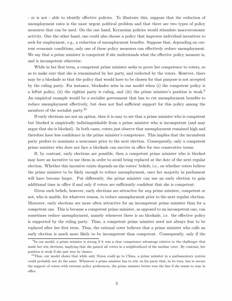
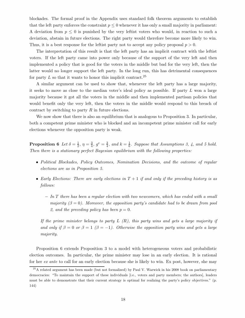
The following graph shows the utility difference UN (θ) − UE(θ) under the assumption that

ge = 34 . Voter types for which this difference takes a positive value are better off in a system

with fixed election timing. Given ge = 34 , the graph shows that almost every voter type, with

the exception of those in a small neighborhood of the median, would prefer a constitution that

precludes early elections.

Given the specification of our model, it is reasonable to assume that 0 ≤ ge ≤ 1: The assumption

26See Figure 3 below.

19

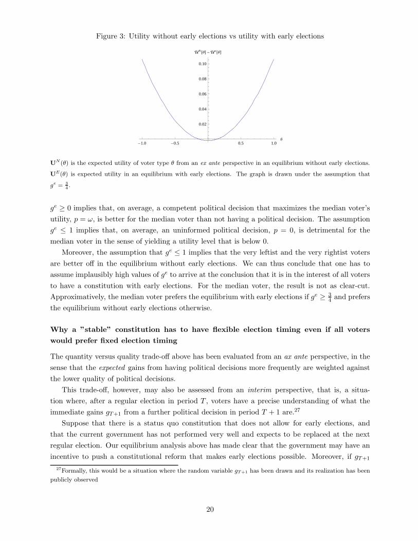
Figure 3: Utility without early elections vs utility with early elections

-1.0 -0.5 0.5 1.0Θ

0.02

0.04

0.06

0.08

0.10

UN @ΘD -Uã@ΘD

UN(θ) is the expected utility of voter type θ from an ex ante perspective in an equilibrium without early elections.

UE(θ) is expected utility in an equilibrium with early elections. The graph is drawn under the assumption that

ge = 3

4.

ge ≥ 0 implies that, on average, a competent political decision that maximizes the median voter’s

utility, p = ω, is better for the median voter than not having a political decision. The assumption

ge ≤ 1 implies that, on average, an uninformed political decision, p = 0, is detrimental for the

median voter in the sense of yielding a utility level that is below 0.

Moreover, the assumption that ge ≤ 1 implies that the very leftist and the very rightist voters

are better off in the equilibrium without early elections. We can thus conclude that one has to

assume implausibly high values of ge to arrive at the conclusion that it is in the interest of all voters

to have a constitution with early elections. For the median voter, the result is not as clear-cut.

Approximatively, the median voter prefers the equilibrium with early elections if ge ≥ 34 and prefers

the equilibrium without early elections otherwise.

Why a ”stable” constitution has to have flexible election timing even if all voters

would prefer fixed election timing

The quantity versus quality trade-off above has been evaluated from an ax ante perspective, in the

sense that the expected gains from having political decisions more frequently are weighted against

the lower quality of political decisions.

This trade-off, however, may also be assessed from an interim perspective, that is, a situa-

tion where, after a regular election in period T , voters have a precise understanding of what the

immediate gains gT+1 from a further political decision in period T + 1 are.27

Suppose that there is a status quo constitution that does not allow for early elections, and

that the current government has not performed very well and expects to be replaced at the next

regular election. Our equilibrium analysis above has made clear that the government may have an

incentive to push a constitutional reform that makes early elections possible. Moreover, if gT+1

27Formally, this would be a situation where the random variable gT+1 has been drawn and its realization has been

publicly observed

20

is sufficiently high, then this proposal will also be popular: it is supported by voters, who feel a

strong urgency to have a political decision right now, rather than after the next regular election.28

This situation may arise even though, from an ex ante perspective, voters would be happy to tie

their hands so as to have a constitution that never allows for early elections and, moreover, does

not allow for future revisions of this constitutional choice.

Certainly, there will occasionally be circumstances where politicians would love to take advan-

tage of an early election in order to gamble for additional time in office. If, at the same time, in

the general public, the feeling prevails that policy measures need to be taken today rather than

tomorrow, a proposal to change the constitution would find sufficient support.

5 Discussion

In almost all parliamentary democracies, election timing is at the discretion of the government.

Early elections, or snap elections, are triggered mainly for two reasons. Either the government

simply wants to capitalize on its favorable relative standing, compared to the opposition, and gain

more time in office. Or it wants to overcome a blockade in parliament. In our paper, and in contrast

to the existing literature, we have constructed a model in which both reasons for early elections are

possible and can even be present simultaneously. We have done so by taking into account that a

political blockade might also be provoked or staged by a prime minister who wants to trigger early

elections simply in order to gamble for more time in office.

The focus of our analysis has been on welfare implications. We have investigated which voters

benefit and which voters lose from having a constitution that allows for early elections, as opposed

to one where the timing of elections is inflexible.

In the illustrative model, presented in Section 2, we have found that in parliamentary systems

with fixed election timing, competent prime ministers are too often replaced, since once a political

blockade occurs, they cannot act on their own authority any more. This result, at a first glance,

makes plausible the widespread intuition that the government’s right to dissolve parliament is a

necessary antidote to the veto right of the parliament, counterbalancing powers of the executive

and the legislative branch.

To see whether the government’s dissolution right does indeed fulfill this function, we have

extended the illustrative model in section 2 to include the possibility of early elections. There, we

have addressed the question whether voters can separate competent but blocked prime ministers

who call for an early election to force their supposedly welfare-enhancing policy through parliament

from incompetent prime ministers who call for early elections simply to gamble for more time in

office. If this question had been answered affirmatively, this would have been a clear advantage of a

constitution that allows for early elections. However, we have found that it is impossible for voters

to discern the true motives behind an early election. Moreover, incompetent prime ministers call for

early elections more often than competent prime ministers, so that the average quality of political

decisions is lower in a system with flexible election timing. These results have been reproduced in

the fully fleshed model presented in section 4.

28Note that these voters may perfectly foresee how the constitutional change affects political outcomes in the future,

i.e., the argument does not rely on shortsightedness of voters.

21

Thus, if the quality of political decisions was the only issue at stake, a constitutional ban on early

elections would be clearly favorable to voters. However, early elections also influence the timing

of political decisions: Important political decisions are made earlier in the legislative term, when

the next election campaign is still in the distant future; and consequently, more frequent elections

induce a higher frequency of salient policy measures. Thus, in a system in which voters often believe

that “something must be done immediately” by the government, allowing for early elections might

be welfare-enhancing for at least a part of the electorate. However, as we have demonstrated in

Section 4, this scenario is rather unlikely to manifest itself if our model is adequate: Only a rather

high and frequent urgency of political issues can offset the low average quality of political measures

implemented after early elections. In general, it is more likely that voters would be better off in a

parliamentary democracy that has a constitutional ban on early elections.

Thus, our negative answers to the normative question whether early elections are desirable lead

to a positive question: Why do most parliamentary democracies mandate the government with the

right of calling for an early election?

At the end of Section 4, we have given a tentative answer to this: Due to time-consistency

problems, a constitution that bans early elections would be difficult to maintain in a parliamentary

democracy. Even if voters perfectly know that in the long run, they would be better off without

early elections, there will arise a situation at some point in time when voters would prefer imme-

diate action over competent action. At this point of time, a government that fails - deliberately

or not - to be supported by a majority in parliament can and will convince voters to change the

constitution and have early elections.

We finally add some remarks on the empirical plausibility of our model. Our model assumes that

a government is possibly blocked by parliament, and that the outcome of an election determines

whether or not this is likely to happen. In particular, the election outcome determines whether or

not the position of the government relative to the parliament is strong or weak.

Such an analysis does not apply to a presidential system where the position of the government

is strong by constitution. For instance, one might argue that the President of the U.S., who is

elected directly by the people, has a stronger position relative to the two chambers of parliament,

than, say, the German Chancellor, who is elected by the members of parliament. This might well

explain why the U.S. president is less able to attribute lack of political success to a lack of support

in parliament. Moreover, if this is true, then our analysis suggests that there is no scope for early

elections in country like the U.S. A strong government that would seek an early election, possibly

via a constitutional reform, would prove itself to be incompetent, and therefore refrains from such a

course of action. This reasoning might explain why early elections are widespread in parliamentary

democracies, but not in presidential systems.

Most parliamentary democracies, with the exception of Great Britain, are multi-party systems

in which governments typically consist of coalitions of different parties. Although we consider only

single-party governments, the parties L and R in our model can also be interpreted as “fixed”

coalitions, i.e., coalitions of one large and one small party that do not have or consider alternative

coalition partners.

In particular, our analysis is perfectly consistent with the frequent occurrence of political con-

22

flicts within coalition governments. In our model, the fact that voters have heterogenous preferences

implies that the ruling party has to balance the policy preferences of its extreme supporters, on

the one hand, and its supporters close to the median voter, on the other hand. Particularly, if

the ruling party’s majority is small, it attributes its victory to the support of the extreme voters

and hence can accept policy proposals only if they are sufficiently attractive to this clientele. By

contrast, if, say, party L managed to gain voters to the right of the median and therefore rules

with a large majority, then it has to deliver policies that appeal to the voters close to the median.

A small majority in our model therefore resembles a coalition government whose stability relies on

the support of an extreme party, and a large majority resembles a coalition government by several

parties who are oriented towards the center.

With this interpretation of a small majority government as an ideologically diverse coalition

government, and a large majority government as one that is ideologically homogeneous, we can find

empirical support for our assumption that only the former give rise to blockades and to early elec-

tions. Particularly, Warwick (2008) has shown empirically in Chapter 4 of his book that ideological

diversity within the members of a government does have a negative effect on its duration.29

References

Alesina, A. and Tabellini, G. (2007). Bureaucrats or politicians? Part 1: A single policy task.

American Economic Review, 97:169–179.

Balke, N. (1990). The rational timing of parliamentary elections. Public Choice, 65:201–216.

Baron, D. and Fehrejohn, J. (1989). Bargaining in legislatures. American Political Science Review,

83:1181–1206.

Battaglini, M. (2010). Dynamic electoral competition and constitutional design. Mimeo.

Battaglini, M. and Coate, S. (2008a). A dynamic theory of public spending, taxation and debt.

American Economic Review, 98:201–236.

Battaglini, M. and Coate, S. (2008b). Pareto-efficient income taxation with stochastic abilities.

Journal of Public Economics, 92:844–868.

Battaglini, M., N. S. and Palfrey, T. (2010). Political institutions and the dynamics of public

investment. Mimeo.

Chapell, D. and Peel, D. (1979). On the political theory of the business cycle. Economics Letters,

2:327–332.

Dewatripont, M., Jewitt, I., and Tirole, J. (1999a). The economics of career concerns. Part 1:

Comparing information structures. Review of Economic Studies, 66:183–198.

29Among empiricists, the opinion has long been cherished that minimal winning governments survive longer than

governments with a clear majority in parliament. Again, Warwick (2008) provides an empirical justification of our

modelling. He has shown that the received opinion is false: If suitable measures of ideological diversity between

government members are included as explanatory variables, the effect of the size of the majority on the duration of

the government becomes insignificant.

23

Dewatripont, M., Jewitt, I., and Tirole, J. (1999b). The economics of career concerns. Part 2:

Application to missions and accountability of government agencies. Review of Economic Studies,

66:199–217.

Diermeier, D. and Merlo, A. (2000). Government turnover in parliamentary democracies. Journal

of Economic Theory, 94:46–79.

Fahri, E. and Werning, I. (2008). The political economy of non-linear capital taxation. Mimeo,

MIT.

Fu, Q. and Li, M. (2010). Policy making with reputation concerns. CIREQ Working Paper, No.

09-2010.

Holmstrom, B. (1999). Managerial incentive problems: A dynamic perspective. Review of Economic

Studies, 66:169–182.

Kayser, M. (2005). Who surfs, who manipulates? the determinants of opportunistic election timing

and electorally motivated economic intervention. American Political Science Review, 99:17–28.

Keppo, J., Smith, L., and Davydov, D. (2008). Optimal electoral timing: Exercise wisely and you

may live longer. Review of Economic Studies, 75:597–628.

Lachler, U. (1982). On political business cycles with endogenous election dates. Journal of Public

Economics, 17:111–117.

Lupia, A. and Strom, K. (1995). Coalition termination and the strategic timing of parliamentary

elections. American Political Science Review, 89:648–665.

Martin, L. W. (2004). The government agenda in parliamentary democracies. American Journal

of Political Science, 48:445–461.

Persson, T. and Tabellini, G. (2000). Political Economics. MIT Press, Cambridge, MA.

Persson, T. and Tabellini, G. (2003). The Economic Effects of Constitutions. MIT Press, Cam-

bridge, MA.

Smith, A. (2004). Election Timing. Cambridge University Press.

Warwick, P. V. (2008). Multiparty Democracy. Cambridge University Press.

A Appendix

Proof of Proposition 1

The proof proceeds in two steps. We first derive an expression for the expected utility of voters in

the hypothesized equilibrium (Lemma 1). Subsequently, we verify the claims made in Proposition

1 (Lemmas 2-4).

24

Lemma 1 Suppose that Proposition 1 is true. Then the expected utility, UN , of a voter prior to

an election where both parties are nominating a newcomer equals

UN =−3

4

1 − 34δ2 − 1

4δ4. (2)

Proof Since both parties have an equal winning probability if they both nominate a newcomer,

UN =1

2UNL +

1

2UNR (3)

where UNJ is expected utility conditional on a victory of party J ∈ {L,R}. Since the prime

minister is competent with probability 12 ,

UNJ =1

2UNJc +

1

2UNJi (4)

where UNJt is expected utility conditional on a victory of party j and prime minister type t ∈ {c, i}.

Since a type i prime minister generates u = −1 and is not nominated again,

UNJi = −1 + δ2UN , (5)

for each J .

Now suppose that the prime minister is competent. Then with probability 12 he generates u = 0

in his first period, is reelected and produces the same outcome also in the next period. Otherwise,

the outcome is u = −1 in the first period, and the subsequent election is one with two newcomers.

Hence, for each J ,

UNJc =1

2(−1 + δ2UN ) +

1

2δ4UN (6)

Equations (3)-(6) imply equation (2).

Lemma 2 Suppose that the ruling party nominates the prime minister for a second election only

if she previously generated the outcome u = 0. Then, if the prime minister is competent and in her

last period, the policy outcome is u = 0. If the prime minister is competent and in her first period,

the outcome is u = 0 if and only if D implements p = ω. In all other cases, the outcome is u = −1.

Proof An incompetent prime minister cannot condition on the current value of ω, and hence

always delivers u = −1. Now consider a competent prime minister. Suppose she is in her last term,

so that she no longer has career concerns and, moreover, can implement all policies. Consequently,

she chooses p = ω and u = 0. If she is in her first term, she can ensure a second nomination only

if she is competent and the device D implements p = ω. She will hence pick p = ω, whenever D

implements it.

Lemma 3 Suppose a candidate has already proven to be competent and competes against a new-

comer. Then the competent candidate is nominated by her party and wins with certainty.

25

Proof If the competent candidate wins, this yields an expected utility of δ2UN for the voters. If

the newcomer wins, he will be able to implement any policy he likes. Consequently, the outcome

is u = −1 if the newcomer is competent, and the newcomer’s part will not nominate her a second

time. Otherwise the outcome is u = 0 and she will be renominated. The voters’ expected utility if

the newcomer wins equals

1

2

(−1 + δ2UN

)+

1

2δ4UN

It is straightforward to show that this expression is smaller than δ2UN , for all δ ∈ (0, 1). Hence, the

incumbent wins so that the incumbent’s party prefers to renominate the incumbent over nominating

a newcomer who would only win with probability 12 .

Lemma 4 A party nominates a newcomer if the previous outcome was u = 0.

Proof Suppose the incumbent can be nominated again, and that the previous outcome was

u = 0. By Bayes’ rule, the probability that an incumbent who has generated the outcome u = 0 is

competent is given by

Pr(u = −1 | comp.) Pr(comp.)

Pr(u = −1 | comp.) Pr(comp.) + Pr(incomp.)=

1

3,

If the incumbent is reelected the expected utility equals −23 + δ2UN . This is smaller than the

expected utility with a newcomer 12

(−1 + δ2UN

)+ 1

2δ4UN .

Proof of Proposition 2

The proof proceeds in two steps. We first derive an expression for the expected utility of voters in

the hypothesized equilibrium (Lemma 5). Subsequently, we verify the claims made in Proposition

2.

Lemma 5 Suppose that Proposition 2 is true. The expected utility, UE, of a voter in an equilibrium

with early elections prior to an election where both parties are nominating a newcomer equals

UE = −

(34 + 1

4δ)

1 − 38δ2 − 3

8δ3 − 14δ4

. (7)

Proof Since both parties have an equal winning probability if they both nominate a newcomer,

UE =1

2UEL +

1

2UER (8)

where UEJ is expected utility conditional on a victory of party J ∈ {L,R}. Since the prime minister

26

is competent with probability 12 ,

UEJ =1

2UEJc +

1

2UEJi (9)

where UEJt is expected utility conditional on a victory of party J and prime minister type t ∈ {c, i}.

A type i prime minister generates u = −1 and initiates early elections whenever the opposition

party’s candidate has to be drawn from pool 2. Otherwise she stays in office until T + 2, where she

is not nominated again,

UEJi = −1 +1

2δ2UE +

1

2

(−δ + δ3UE

), (10)

for each J .

If the prime minister is competent, she can generate u = 0 with probability 12 . In this case she

will be nominated again and win with certainty. Otherwise, the outcome is u = −1, and there is

an is an early election with probability 12 . Hence,

UEJc =1

2δ4UE +

1

2

(−1 +

1

2δ2UE +

1

2δ3UE

). (11)

Equations (8)-(11) imply equation (7).

Lemma 6 Given the behavior of voters in early and regular elections and the nomination decision

of parties, in any period where a political decision is taken, the policy outcome is u = 0 if the prime

minister is competent and D implements p = ω, and u = −1 otherwise.

Proof If the prime minister is competent and in her second period, this follows because she seeks

to maximize the voters’ utility, and D implements p = ω. If she is incompetent and in her second

period, u = −1 follows because the prime minister cannot condition her policy proposal on ω.

Now suppose she is in her first period. If she is competent and D implements p = ω, proposing

p = ω implies that she will be nominated again and reach the maximum time in office because her

type will be revealed prior to the next regular election.

Now suppose she is incompetent or D does not implements p = ω. In this case the outcome

u = −1 results necessarily.

Lemma 7 Consider a regular election in T + 2 where the prime minister can be nominated for a

second term. It is optimal to nominate the prime minister if and only if uT = 0.

Proof If uT = 0, then it has been revealed that the prime minister is competent. If she is

nominated her party wins with certainty. The argument is as follows. The voters expected payoff

if the incumbent wins equals δ2UE. If the newcomer wins against the incumbent, D implements

any policy proposal. Hence, if the newcomer is competent he will be able to prove it and he

will be elected one more time, at the next regular election. Otherwise is incompetence is proven

(the outcome u = −1 can be attributed only to a lack of competence if D implements any policy

27

proposal) and he will be replaced at the next regular election. The expected payoff from a newcomer

therefore equals 12(−1+δ2UE)+ 1

2δ4UE . It is straightforward to verify that this expression is smaller

than δ2UE .

If uT = −1, then the arguments from the Proof of Proposition 1 imply that the incumbent

is competent with probability 13 . The expected utility if the incumbent wins is thus −2

3 + δ2UE,

which is smaller than the payoff if the newcomer wins.

Lemma 8 A prime minister who is in first period, competent and able to implement p = ω does

not initiate early elections. Suppose δ < 23 . Then, a prime minister who who is unable to implement

p = ω. chooses early elections if and only if the opposition party’s candidate has to be drawn from

pool 2.

Proof If the prime minister is competent she can reach the maximum time in office if and only if

she proposes p = ω in her first period and does not initiate early elections.

In the following, consider a prime minister who is unable to implement p = ω. In the hypoth-

esized equilibrium, Bayes’ rule implies that conditional on the events “early elections take place”

the probability that the prime minister is competent equals 13 .

Suppose first that the incumbent competes against a newcomer from the opposition party who

is drawn from pool 2 and is hence competent with probability k. Hence voters get an expected

payoff of −23 + δ2UE if the incumbent wins.

If the newcomer wins they get γδ4UE + (1 − γ)(−1 + δ2UE

), where γ = 1

2 if the newcomer is

drawn form pool 1 and γ = k if the newcomer is drawn form pool 2.

It is straightforward to verify that γ = 12 implies that voters prefer the newcomer. Hence, in

this case the incumbent prefers not to have an early election. Thereby she remains in office until

T + 2, rather than being replaced in T + 1.

For γ = k, voters prefer that the incumbent wins if and only if

k <1

3(1 − (δ2 − δ4)UE

Obviously, for δ sufficiently large, this inequality is satisfied for k = 16 . Hence, the incumbent

prefers to have an early election. Thereby she remains in office until T + 3, rather than being

replaced in T + 2.

Proof of Proposition 4

The derivation of CN , and PN follows from the same line of reasoning as the derivation of UN in

Lemma 1 and yields the following expressions:

CN =1 + δ + 1

4 (δ2 + δ3)

1 − 34δ2 − 1

4δ4and PN =

1

1 − δ2.

The derivation of CE, and PE parallels the derivation of UE in Lemma 5:

CE =1 + δ + 1

4(δ2 + δ3) + 38δ2

1 − 38δ2 − 3

8δ3 − 14δ4

and PE =1 + 3

8δ + 14δ2

1 − 38δ2 − 3

8δ3 − 14δ4

.

28

It is now straightforward to verify that CN > CE, and PE > PN .

Proof of Proposition 5

The proof proceeds in three steps. We first compute the utility of voters in the hypothesized

equilibrium (Lemma 9). For the second step, we take it as given that political blockades occur and

show that the prime minister’s policy proposals, the party’s nomination decisions and the behavior

of voters are mutually best responses (Lemmas 10 - 12). In the final step, we endogenize the

political blockade (Lemmas 13 and 14).

Lemma 9 Suppose that Proposition 5 is true. The expected utility, UN (θ), of voter type θ prior to

an election where both parties are nominating a newcomer and prior to learning the next period’s

g equals

UN (θ) =(ge

−3θ2)(1+ 1

2δ2)− 1

2

1− 1

2δ4

−1

2δ2

. (12)

Proof We first compute the continuation utility UN (θ) of a voter with type θ prior to an election

campaign (i.e., before observing β) where both parties nominate a newcomer and prior to observing

the next period’s realization of g.

Suppose that both parties compete with a newcomer. We will verify below that β = 1 (β = −1)

implies that party L (R) wins with a large majority and that β = 0 implies that either party wins

with probability 12 and has only a small majority in case of winning. It is straightforward to verify

that all of these events occur with equal probability. Hence,

UN (θ) = 14 [Ll(θ) + Ls(θ) + Rs(θ) + Rl(θ)] (13)

where Ll(θ) is the continuation utility if party L wins with a large majority and Ls(θ) is the

continuation utility that applies if the majority is small. Rl(θ) and Rs(θ) are defined in the same

way.

The payoff given that party L wins with a large majority is based on expectations about the

prime minister’s type conditional on the event β = 1,

Ll(θ) = Pr(tL = c | β = 1)Llc(θ) + Pr(tL = i | β = 1)Lli(θ)

= ηLlc(θ) + (1 − η)Lli(θ) .(14)

Llc(θ) (Lli(θ)) is the expected continuation utility conditional on the events β = 1 and tL = c

(tL = i). In the hypothesized equilibrium, a competent prime minister stays in office for two

periods because in case of having a large majority she can reveal her type during her first term

with probability 1, by implementing the policy p = ω. This implies

Llc(θ) = (1 + δ2)(ge − 3θ2) + δ4UN (θ) . (15)

By contrast, an incompetent politician stays in office for only one period, and the implemented

policy is p = 0. Since his type becomes common knowledge the party nominates a newcomer in

29

the next regular election. This implies

Lli(θ) = (ge − 3θ2 − 1) + δ2UN (θ) , (16)

where 3θ2 + 1 = E[λ(p, ω, θ) | p = 0, p 6= ω].

If party L wins with a small majority, then, the continuation utility Ls(θ) is given by

Ls(θ) = Pr(tL = c | β = 0)Lsc(θ) + Pr(tL = i | β = 0)Lsi(θ)

= 12Lsc(θ) + 1

2Lsi(θ) ,(17)

where Lsi(θ) = Lli(θ) because the behavior of an incompetent politician does not depend on the

size of the majority. By contrast, a competent politician can choose p = ω if ω ≤ 0 and has to

choose p = 0 otherwise. Hence,

Lsc(θ) = Pr(ω ≤ 0)Lscnb(θ) + Pr(ω > 0)Lsc

b (θ)

= 12Llc(θ) + 1

2Lscb (θ) ,

(18)

where Lscb (θ) is the continuation utility that applies if the president is blocked. In an equilibrium

without early elections,

Lscb (θ) = (ge − 3θ2 − 3θ − 1) + δ2UN (θ) . (19)

where 3θ2 + 3θ + 1 = E[λ(p, ω, θ) | p = 0, ω > 0].

Likewise, one can derive the corresponding expressions for Rs(θ) and Rl(θ). Substituting the

resulting formulas into (13) and using the assumption η = 34 yields equation (12).

Taking the political blockades as given, it follows from Lemma 2 that the policy outcome in

any period is p∗ = ω if the prime minister is competent and if there is no blockade, and p = 0

otherwise.

Lemma 10 Consider a regular election where two newcomers are running. Party L (R) wins with

a large majority if and only if β = 1 (β = −1). If β = 0, then the winning party has a small

majority, and each party wins with probability 12 .

Proof

Case 1. Suppose the election campaign ends with a signal in favor of the left candidate β = 1. We

show in the following that, conditional on this event, for a majority of voters a large majority for

party L is the preferred outcome of the election.

Step 1. Consider first the comparison between a large majority for party L and a large majority

for party R. Given the posterior beliefs, the expected utility if L wins a large majority is given by

Ll(θ) whereas the expected utility if party R wins a large majority is given by

(1 − η)Rlc(θ) + ηRLi(θ) ,

30

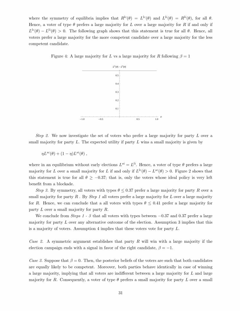
where the symmetry of equilibria implies that Rlc(θ) = Llc(θ) and Lli(θ) = Rli(θ), for all θ.

Hence, a voter of type θ prefers a large majority for L over a large majority for R if and only if

Llc(θ) − Lli(θ) > 0. The following graph shows that this statement is true for all θ. Hence, all

voters prefer a large majority for the more competent candidate over a large majority for the less

competent candidate.

Figure 4: A large majority for L vs a large majority for R following β = 1

-1.0 -0.5 0.5 1.0Θ

0.1

0.2

0.3

0.4

0.5

Llc@ΘD - Lli@ΘD

Step 2. We now investigate the set of voters who prefer a large majority for party L over a

small majority for party L. The expected utility if party L wins a small majority is given by

ηLsc(θ) + (1 − η)Lsi(θ) ,

where in an equilibrium without early elections Lsi = Lli. Hence, a voter of type θ prefers a large

majority for L over a small majority for L if and only if Llc(θ) − Lsc(θ) > 0. Figure 2 shows that

this statement is true for all θ ≥ −0.37; that is, only the voters whose ideal policy is very left

benefit from a blockade.

Step 3. By symmetry, all voters with types θ ≤ 0.37 prefer a large majority for party R over a

small majority for party R . By Step 1 all voters prefer a large majority for L over a large majority

for R. Hence, we can conclude that a all voters with types θ ≤ 0.41 prefer a large majority for

party L over a small majority for party R.

We conclude from Steps 1 - 3 that all voters with types between −0.37 and 0.37 prefer a large

majority for party L over any alternative outcome of the election. Assumption 3 implies that this

is a majority of voters. Assumption 4 implies that these voters vote for party L.

Case 2. A symmetric argument establishes that party R will win with a large majority if the

election campaign ends with a signal in favor of the right candidate, β = −1.

Case 3. Suppose that β = 0. Then, the posterior beliefs of the voters are such that both candidates

are equally likely to be competent. Moreover, both parties behave identically in case of winning

a large majority, implying that all voters are indifferent between a large majority for L and large

majority for R. Consequently, a voter of type θ prefers a small majority for party L over a small

31

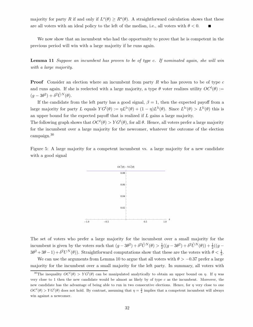
majority for party R if and only if Ls(θ) ≥ Rs(θ). A straightforward calculation shows that these

are all voters with an ideal policy to the left of the median, i.e., all voters with θ < 0.

We now show that an incumbent who had the opportunity to prove that he is competent in the

previous period will win with a large majority if he runs again.

Lemma 11 Suppose an incumbent has proven to be of type c. If nominated again, she will win

with a large majority.

Proof Consider an election where an incumbent from party R who has proven to be of type c

and runs again. If she is reelected with a large majority, a type θ voter realizes utility OC l(θ) :=

(g − 3θ2) + δ2UN (θ).

If the candidate from the left party has a good signal, β = 1, then the expected payoff from a

large majority for party L equals Y Gl(θ) := ηLlc(θ) + (1 − η)Lli(θ). Since Llc(θ) > Lli(θ) this is

an upper bound for the expected payoff that is realized if L gains a large majority.

The following graph shows that OC l(θ) > Y Gl(θ), for all θ. Hence, all voters prefer a large majority

for the incumbent over a large majority for the newcomer, whatever the outcome of the election

campaign.30

Figure 5: A large majority for a competent incumbent vs. a large majority for a new candidate

with a good signal

-1.0 -0.5 0.5 1.0Θ

0.02

0.04

0.06

0.08

OCl@ΘD -YGl

@ΘD

The set of voters who prefer a large majority for the incumbent over a small majority for the

incumbent is given by the voters such that (g − 3θ2) + δ2UN (θ) > 12((g − 3θ2) + δ2UN (θ)) + 1

2((g −

3θ2 +3θ−1)+ δ2UN (θ)). Straightforward computations show that these are the voters with θ < 13 .

We can use the arguments from Lemma 10 to argue that all voters with θ > −0.37 prefer a large

majority for the incumbent over a small majority for the left party. In summary, all voters with

30The inequality OCl(θ) > Y Gl(θ) can be manipulated analytically to obtain an upper bound on η. If η was

very close to 1 then the new candidate would be almost as likely by of type c as the incumbent. Moreover, the

new candidate has the advantage of being able to run in two consecutive elections. Hence, for η very close to one

OCl(θ) > Y Gl(θ) does not hold. By contrast, assuming that η = 3

4implies that a competent incumbent will always

win against a newcomer.

32

types between −0.37 and 0.33 prefer a large majority for the incumbent over any other outcome.

By assumptions 3 and 4 this implies that the incumbent wins with a large majority.

Now suppose that the policy outcome has been p = 0. From the perspective of voters this

indicates that either there has been a blockade – conditional on this event the prime minister is

competent with probability 12 – or there has not been a blockade and prime minister is incompetent

with probability 1. The arguments in the proof of Lemma 4 imply that in this situation all voters

with preferences in a neighborhood of the median would prefer a large majority for the newcomer

over any other outcome if the prime minister was nominated again, which implies that the prime

minister’s party prefers to nominate a newcomer. This is summarized in the following Lemma,

which we state without proof.

Lemma 12 Suppose an incumbent has implemented p = 0. If nominated, the other candidate will

win with a large majority.

We now turn to the incentives of parties to enact political blockades. Without loss of generality,

we study only the incentives for the left party. We first derive the left party’s payoffs in equilibrium.

Prior to an election campaign with two newcomers, the left party’s payoff VL is given by

VL =1

4(SLl

L + SLsL + SRl

L + SRsL ) , (20)

where SLlL is the expected payoff of party L conditional on winning a large majority in a regular

election where two newcomers are running. SLsL is the expected payoff in case of winning a small

majority. SRlL and SRs

L are the payoffs of the left party if the right party wins. We have that

SLlL = η(1 + δ + δ2 + δ3 + δ4VL) + (1 − η)(1 + δ + δ2VL)

SLsL =

1

2(1 + δ + δ2 + δ3 + δ4VL) +

1

2(1 + δ + δ2VL)

SRlL = ηδ4VL + (1 − η)δ2VL

SRlL =

1

2δ4VL +

1

2δ2VL .

Substituting these expressions into (20) yields

VL =1 + δ + 1

2(η + 12 )(δ2 + δ3)

2 − (η + 12)δ4 − (3

2 − η)δ2, (21)

It is now straightforward to verify that

VL =1

2

1

1 − δ. (22)

Intuitively, this is the present value of an infinite stream of expected per period payoffs of 12 , where

12 the probability to be in office in any one period.

Lemma 13 Suppose L has a small majority. It is optimal for the party to block any policy p ≥ 0

if it expects that otherwise leftist voters would abstain in the future whenever there is an election

where both parties nominate a newcomer and β = 0.

33

Proof Suppose there is an alternative equilibrium where leftist voters abstain whenever β = 0

and, as a consequence, party R gains a large majority whenever β = 0. In all other cases voting

behavior is unaffected. In this alternative equilibrium the left party’s payoff VLA is given by

VLA =1

4(SLl

LA + SLsLA + SRl

LA + SRsLA) , (23)

where

SLlLA = η(1 + δ + δ2 + δ3 + δ4VLA) + (1 − η)(1 + δ + δ2VLA)

SLsLA =

1

2δ4VLA +

1

2δ2VLA

SRlLA = ηδ4VLA + (1 − η)δ2VLA

SRlLA =

1

2δ4VLA +

1

2δ2VLA .

Substituting these expressions into (23) yields

VLA =12(1 + δ) + 1

2η(δ2 + δ3)

2 − (η + 12)δ4 − (3

2 − η)δ2, (24)

Assuming that a deviation affects future play of leftist voters, the maximal utility that the left

party can obtain by deviating from blocking any policy p ≥ 0 is given by

1 + δ + δ2 + δ3VLA .

This is based on the assumption that the party can win the next regular election by deviating.

Thereafter, the party has to nominate a newcomer and from then one the new equilibrium payoff

becomes relevant. By contrast, if the party honors its implicit contract with leftist voters, then the

payoff is given by

1 + δVL .

Straightforward calculations show that for η = 34 and for δ = 1

2 we have that

1 + δVL > 1 + δ + δ2 + δ3VAL .

This implies that the left party has no incentive to deviate.

Using the same argument, one can show that it is not in the party’s interest to deviate from

moving as close as possible to the median voter’s preferred policy. Suppose that the party and

the prime minister would consider a deviation such that in one period a policy that is optimal for

voters with types to the left of the median is implemented. If this implies that in future elections

all voters in a neighborhood of the median vote for party R whenever the race is close, such a

deviation is not attractive.

Lemma 14 Consider a deviation of party L that yields a short run gain for leftist voters. If this

34

implies that in the future voters in the middle vote for party R whenever there is an election where

both parties nominate a newcomer and β = 0, then such a deviation is not attractive.

Proof of Proposition 6

The proof proceeds in three steps. We first consider the incentives for a prime minister to call

for early elections. Lemma 15 shows that after the early election campaign, voters may consider

the opposition party’s candidate to be more competent. Lemma 16 shows that the prime minister

may want to call an early election even if the opposition party will exactly in those circumstances

where the newcomer outperforms the incumbent in the early election campaign. Second, we derive

voter utility in the hypothesized equilibrium (Lemma 17). Finally, we explain the steps that are

required to verify that the hypothesized behavior constitutes indeed a stationary perfect Bayesian

equilibrium.

Lemma 15 Let the history of events be as follows: Consider an early election with campaign

outcome β′ that takes place after voters have observed p = 0, an opposition party’s candidate who

has been drawn from pool 2, and a preceding regular election with two newcomers who tied in the

election campaign, β = 0. Suppose the prime minister belongs to party L. If 13 > k >

(1−η)2

(1−η)2+2η2 ,

then Pr(tL = c | β′) > Pr(tR = c | β′) if β = 1 or β = 0, and Pr(tL = c | β′) < Pr(tR = c | β′), if

β = −1.

Proof The probability that the prime minister is competent equals 13 , as in the illustrative model

in Section 3.

Case 1. Suppose that β′ = 0. By definition of a conditional probability

Pr(tL = c | β′ = 0) =13Pr(β′ = 0 | tL = c)

13Pr(β′ = 0 | tL = c) + 2

3Pr(β′ = 0 | tL = i). (25)

The assumption that αL and αR are independent random variables implies that

Pr(β′ = 0 | tL = c) = η[kη + (1 − k)(1 − η)] + (1 − η)[k(1 − η) + (1 − k)η] , (26)

and

Pr(β′ = 0 | tL = i) = (1 − η)[kη + (1 − k)(1 − η)] + η[k(1 − η) + (1 − k)η] . (27)

Combining equations (25) - (27) yields

Pr(tL = c | β′ = 0) =13{2η(1 − η) + k(2η − 1)2}

−13k(2η − 1)2 + 2

3{(1 − η)2 + η(1 − η) + η2}. (28)

In a similar way we derive

Pr(tR = c | β′ = 0) =k

[13{η

2 + (1 − η)2} + 23{2η(1 − η)}

]

−13k(2η − 1)2 + 2

3{(1 − η)2 + η(1 − η) + η2}. (29)

35

It follows from equations (29) and (28) that

Pr(tL = c | β′ = 0) > Pr(tN = c | β′ = 0) ⇐⇒ k < 13 .

Case 2. Suppose that β′ = 1. Using the same arguments as in Case 1, we derive

Pr(tL = c | β′ = 1) =η

2 − η. (30)

and

Pr(tN = c | β′ = 1) =k

[13η(1 − η) + 2

3(1 − η)2]

13(2 − η){k(1 − η) + (1 − k)η}

(31)

It follows that,

Pr(tL = c | β′ = 1) > Pr(tN = c | β′ = 1) ⇐⇒ k < η2

2+3η2−4η

.

With η = 34 , η2

2+3η2−4η

> 16 . It follows that Pr(tL = c | β′ = 1) > Pr(tN = c | β′ = 1).

Case 3. Suppose that β′− = 1. Using the same arguments as Case 1, we derive

Pr(tL = c | β′ = −1) =1 − η

1 + η. (32)

and

Pr(tN = c | β′ = −1) =k

[13η(1 − η) + 2

3η2]

13(1 + η){kη + (1 − k)(1 − η)η}

(33)

It follows that,

Pr(tL = c | βEE = −1, EE, k) < Pr(tN = c | βEE = −1, EE, k)

⇐⇒ k >(1−η)2

(1−η)2+2η2

Lemma 16 Suppose the prime minister belongs to party L. Suppose there is a blockade or that the

prime minister is incompetent. Suppose that the opposition party’s candidate is drawn from pool

2, and that the preceding regular election in period T had β = 0. Suppose that the prime minister

would not be nominated again if there was a regular election in T + 2. Suppose that the prime

minister will win an early election if and only if β 6= −1. Let (1+ δ)(1−kη2 − (1−k)η(1−η)) > 1,

then it is optimal both for a competent and an incompetent prime minister to call for an early

election.

Proof If the prime minister does not initiate early elections, her payoff as of period T + 1 equals

1 because she can stay in office until T + 2. If she wins an early election her expected payoff equals

(1+ δ)Pr(β′ 6= −1 | tL) because in case of winning she stays in office until T +3 and loses her office

36

otherwise. Suppose first that tL = i. Then,

Pr(β′ = −1 | tL = i) = kPr(β′ = −1 | tR = c, tL = i)

+(1 − k)Pr(β′ = −1 | tR = i, tL = i)

= kη2 + (1 − k)η(1 − η)

Hence, an incompetent prime minister calls for early elections if

(1 + δ)(1 − kη2 − (1 − k)η(1 − η)) > 1 .

Now suppose that the prime minister is competent, then

Pr(β′ = −1 | tL = c) = kη(1 − η) + (1 − k)(1 − η)2

which is strictly smaller than Pr(β′ = −1 | tL = i). Hence a competent prime minister also opts

for early elections.

Lemma 17 Suppose Proposition 6 is true. Then, the expected utility, UE(θ), of voter type θ prior

to an election where both parties are nominating a newcomer and prior to learning the next period’s

g equals

UE(θ) =q(ge − 3θ2) − r

1 − u, (34)

where

q := 1 +3

8ρδ +

(1

8+

1

2η

)δ2 +

1

4ρ

(1

2σc + σi

)δ3,

r :=

(3

8+

1

2(1 − η)

)+

1

4

(αi + γi +

1

2γc

)ρδ,

u :=

(3

8(1 − ρ) +

1

2(1 − η)

)δ2 + ρ

(1

8(αc + γc) +

1

4(αi + γi)

)δ3

+

(1

8+

1

2η

)δ4 + ρ

(1

8σc +

1

4σi

)δ5.

and

αc := Pr(β′ = −1 | tL = c) = 1 − kη(1 − η) − (1 − k)(1 − η)2,

is the probability that a competent incumbent wins an early election and

αi := Pr(β′ = −1 | tL = i) = 1 − kη2 − (1 − k)η(1 − η),

is the probability that an competent incumbent wins. We denote by

σc := Pr(β′ = −1, tR = c | tL = c) = kPr(β′ = −1, | tR = c, tL = c) = kη(1 − η),

the joint probability that the incumbent loses and that the newcomer is competent given that the

incumbent is competent, and by

σi := kη2,

37

the joint probability that the incumbent loses and that the newcomer is competent given that the

incumbent is not competent. Analogously, the joint probability that the incumbent loses and that

the newcomer is incompetent is given by

γc := (1 − η)2(1 − k),

if the incumbent is competent and by

γi := η(1 − η)(1 − k),

if the incumbent is incompetent. Finally ρ = 12 is the probability that the opposition party’s candidate

has to be drawn from pool 2.

Proof An election where both nominate a newcomer leads to a large majority for party L (R) if

β = 1 (β = −1) which happens with probability 14 . Conditional on β = 0 either party has an equal

chance of winning with a small majority. Hence,

UE(θ) = 14 [Ll(θ) + Ls(θ) + Rs(θ) + Rl(θ)] , (35)

where Ll(θ) is the continuation utility if party L wins with a large majority and Ls(θ) is the

continuation utility that applies if the majority is small, etc.

In case of winning with a large majority, there is no political blockade. Hence,

Ll(θ) = ηLlc(θ) + (1 − η)Lli(θ) , (36)

where

Llc(θ) = (1 + δ2)(ge − 3θ2) + δ4UE(θ) , (37)

and

Lli(θ) = (ge − 3θ2 − 1) + δ2UE(θ) , (38)

Again, by symmetry Ll(θ) = Rl(θ).

If party L wins with a small majority, then, the continuation utility Ls(θ) is given by

Ls(θ) = 12 Lsc(θ) + 1

2 Lsi(θ) , (39)

where

Lsc(θ) = 12 Lsc

nb(θ) + 12 Lsc

b (θ) , (40)

and Lscnb is the continuation utility that applies if ω ≤ 0 and there is no blockade, and Lsc

b is the

continuation utility that applies otherwise. If there is no blockade, a competent prime minister can

prove his competence which implies that

Lscnb(θ) = Llc(θ) (41)

38

With probability 1−ρ there is no early election but a regular election where both parties nominate

a newcomer. Hence,

Lscb (θ) = (ge − 3θ2 − 3θ − 1) + (1 − ρ)δ2UE(θ) + ρXc(θ), (42)

where

Xc(θ) := αc[δ(ge − 3θ2) + δ3UE(θ)] + σcδRlc(θ) + γcδRli(θ)

Analogously, we derive

Lsi(θ) = (ge − 3θ2 − 1) + (1 − ρ)δ2UE(θ) + ρXi(θ) (43)

where

Xi := αi[δ(ge − 3θ2 − 1) + δ3UE(θ)] + σiδRlc(θ) + γiδRli(θ)

The expressions for party R are derived in the same way. Substituting all the resulting expressions

into (35) establishes the Lemma.

The remaining steps to complete the proof of Proposition 6 are similar to those for the proof of

Proposition 5. We therefore only sketch the arguments.31 We first verify that Lemma 10 also holds

in the current setting. The arguments and the results are exactly the same as in the proof of Lemma

10. We further verify that an early election is indeed such that the incumbent wins with a large

majority if β 6= −1 and that the opposition party wins with a large majority otherwise. Therefore

it is necessary to use the appropriate posterior beliefs on candidate competence when computing

expected utility conditional on the outcome of the early election campaign and to adjust for the

fact that the incumbent has a shorter time horizon than the newcomer. Given these modifications,

the arguments and the results which characterize the outcome of early elections are same as in the

proof of Lemma 10. Finally, we show that also Lemmas 11-14 go through.

31Details are available from the authors upon request.

39