Embed Size (px)
Citation preview
POLITECNICO DI TORINO
Corso di Laurea Magistrale
in Ingegneria Energetica e Nucleare
Tesi di Laurea Magistrale
Energy analysis and HVAC system sizing of a mixed
industrial and office Nearly Zero-Energy building
Relatori
Prof. Ing. Marco Carlo Masoero
Ing. Laura Rietto
Candidato
Martina Giometti
Anno Accademico 2017/2018
1
Abstract
The need to have a more eco-sustainable world has steered our daily practices towards more
conscious and rational energy uses. Among these activities, the construction of buildings with
nearly zero energy need and the renovation of the existing ones can certainly have a large impact
from an energy standpoint. In this direction, the "Energy Performance Building Directions"
(EPBD) of 2010 define the concept of a nearly zero-energy building (NZEB), although the
criteria to qualify as NZEB remain ambiguous.
In Italy, the NZEB concept is strongly related to a major use of renewable energy sources to
cover the energy demand of the buildings. In this regard, non-residential buildings represent an
important challenge, especially when old industrial structures, built when energy efficiency
was not a primary issue, need to be converted to other uses and comply with the NZEB
requirements.
This work refers to a building of this kind, a disused industrial structure from 1959 in Corso
Orbassano 402 in Turin. SIGIT, a manufacturer of plastic and rubber components, has planned
to redevelop the building and turn it into its directional and operative headquarter, the
Innovation Square Center (ISC). The aesthetic renovation has been entrusted to the architectural
firm SeArch, while structural renovation and the design of the new HVAC plant has been
assigned to Ferplant s.r.l.
In order to preserve the original concrete structure while complying with the normative
requirements, interventions on the envelope of the building are limited to the change of doors
and windows, and to the addition of insulation coatings on walls, floors and ceiling.
Given this, the HVAC system has to be designed in the most efficient way to guarantee the
compliance with the NZEB requirements. This work addresses this issue and analyses the
optimal sizing of the plant by resorting to both a semi-static evaluation using the software
Edilclima and a dynamic simulation carried out with the program DesignBuilder.
The results of the two models, in terms of power and energy consumption, are then compared
to understand the factors that could potentially cause a dissimilarity in the values of the
calculated energy needs. In addition, to better understand how to achieve energy efficiency, in
a further analysis two different air-conditioning configurations in one important space of the
building are evaluated.
In addition to Edilclima and DesignBuilder, other software packages are used:

2
- SketchUp, to draw the 3D model of the building to be used in DesignBuilder, and Open
Studio plug-in to define thermal zones;
- THERM 7.6, to model two-dimensional heat-transfer effects in a building component where
thermal bridges are of concern.
The thesis was carried out at Ferplant s.r.l offices, based in Chivasso (TO).
3
Table of contents
Abstract ...................................................................................................................................... 1
Table of contents ........................................................................................................................ 3
List of figures ............................................................................................................................. 6
List of tables ............................................................................................................................... 9
1. Normative Framework ...................................................................................................... 11
1.1 The European Directives ........................................................................................... 11
1.1.1 Definitions of “Deep renovation” and “NZEB renovation” .................................... 18
1.2 Italian Regulation .......................................................................................................... 20
1.2.1 Legislative Decrees of the 26th June, 2015 .............................................................. 22
1.2.2 The definition of NZEB in Italy .............................................................................. 23
1.2.3 Requirements for NZEBs ........................................................................................ 25
1.2.4 Italian policies to target building renovations ......................................................... 26
2. The Innovation Square Centre .......................................................................................... 31
2.1 Urban characteristics of the site ................................................................................. 32
2.2 The idea ..................................................................................................................... 32
2.2.1 North-East façade ............................................................................................... 34
2.2.2 Internal space ...................................................................................................... 34
2.2.3 Coffee break & buffet lunch area ....................................................................... 35
2.2.4 Other areas .......................................................................................................... 35
2.3 The renovation ........................................................................................................... 36
3. Software implementation .................................................................................................. 38
3.1 Edilclima .................................................................................................................... 38
3.1.1 Main features ...................................................................................................... 39
3.1.2 Calculation method ............................................................................................ 41
3.1.3 Space cooling power calculation by EC706 ....................................................... 52
3.2 DesignBuilder ............................................................................................................ 53
3.2.1 SketchUp & OpenStudio Plug-in ....................................................................... 53
3.2.2 The simulation engine: EnergyPlus .................................................................... 54
3.2.3 Compliance with requirements ........................................................................... 55
3.3 THERM 7.6 ............................................................................................................... 56
4. Methodology ..................................................................................................................... 57
4.1 Building’s design diagrams and front views ............................................................. 57

4
4.2 Simplifications to model the building ....................................................................... 62
4.2.1 Absence of the central structure ......................................................................... 62
4.2.2 Internal partitions ............................................................................................... 65
4.2.3 Orientation’s definition ...................................................................................... 65
4.3 Definition of building’s components ......................................................................... 66
4.4 Edilclima implementation .......................................................................................... 70
4.4.1 Definition of general data of the building .......................................................... 71
4.4.2 Input of building components, shadings and conditioned zones ........................ 71
4.4.3 Systems definition .............................................................................................. 75
4.4.4 Definition of internal gains ................................................................................ 82
4.5 Dynamic model implementation ............................................................................... 83
4.5.1 3D model creation through SketchUp & OpenStudio plug-in ........................... 83
4.5.2 DesignBuilder implementation .......................................................................... 86
5. Thermal bridges analysis .................................................................................................. 96
5.1 Thermal bridge description ........................................................................................ 99
5.1.1 Definition of the section of analysis ................................................................... 99
5.1.2 Definition of necessary data for the THERM elaboration ............................... 100
5.2 THERM implementation ......................................................................................... 101
5.2.1 Drawing ............................................................................................................ 101
5.2.2 Materials’ definition ......................................................................................... 102
5.2.3 Boundary conditions ........................................................................................ 102
5.2.4 Calculations ...................................................................................................... 104
5.2.5 Results visualization ......................................................................................... 105
5.3 Thermal bridge linear transmittance calculation ..................................................... 108
5.4 Condensation and mould formation test .................................................................. 109
5.4.1 Condensation test ............................................................................................. 109
5.4.2 Mould formation test ........................................................................................ 110
6. Results and conclusion .................................................................................................... 111
6.1 Data setting .............................................................................................................. 111
6.1.1 Definition of ventilation supply and extraction flowrates ................................ 111
6.1.2 Definition of indicators for the calculation of internal heat gains .................... 112
6.2 Design space heating and cooling powers ............................................................... 114
6.3 DesignBuilder outputs ............................................................................................. 118
6.4 Energy evaluations and comparison between models ............................................. 120
5
6.4.1 Dispersions by transmission and ventilation .................................................... 120
6.4.2 Solar and internal heat gains ............................................................................ 123
6.4.3 Site and source energy ...................................................................................... 125
6.5 Comparison between different air conditioning strategies ...................................... 127
6.5.1 VAV and CAV in comparison ......................................................................... 128
6.5.2 Addition of radiant heated floor in the ground floor ........................................ 129
6.6 Law verifications ..................................................................................................... 129
6.7 Conclusion ............................................................................................................... 133
References .............................................................................................................................. 135
Acknowledgments .................................................................................................................. 137

6
List of figures
Figure 1.1 - Timeline for NZEBs implementation according to the 1st EPBD recast ............. 12
Figure 1.2 - De-carbonisation Roadmap till 2050 .................................................................... 13
Figure 1.3 - 2030 Framework for Climate and Energy ............................................................ 14
Figure 1.4 - System boundaries ................................................................................................ 16
Figure 1.5 - Main arguments around NZEBs to be established in the definition ..................... 17
Figure 1.6 - EU-28 dwellings according to construction date .................................................. 19
Figure 1.7 - Expected energy savings in the period 2014-2020 (Mtoe/year of final energy) .. 27
Figure 2.1 - View of the building from above.......................................................................... 31
Figure 2.2 - North-East facade as it is ...................................................................................... 34
Figure 2.3 - North-East facade as by design ............................................................................ 34
Figure 2.4 - Internal Space as it is (left) and the "innovation square" (right) .......................... 35
Figure 2.5 - The new coffee break & buffet lunch area as by design ...................................... 35
Figure 3.1 - The energy balance of the building for heating – UNI/TS 11300-1 [19] ............. 41
Figure 3.2 - Heat exchange by transmission [19] ..................................................................... 45
Figure 3.3 - The energy balance of the building for heating – UNI/TS 11300-2 [19] ............. 47
Figure 3.4 - Surface heat balance ............................................................................................. 55
Figure 3.5 - Therm’s flow ........................................................................................................ 56
Figure 4.1 - Basement’s diagram ............................................................................................. 57
Figure 4.2 - Ground floor's diagram ........................................................................................ 58
Figure 4.3 - First floor's diagram ............................................................................................. 59
Figure 4.4 - Second floor's diagram ........................................................................................ 60
Figure 4.5 - Roof's representation ........................................................................................... 61
Figure 4.6 - North front view .................................................................................................. 61
Figure 4.7 - East front view ..................................................................................................... 61
Figure 4.8 - South front view .................................................................................................. 62
Figure 4.9 - West front view ................................................................................................... 62
Figure 4.10 - Ground floor simplified diagram ....................................................................... 63
Figure 4.11 - First floor simplified diagram ............................................................................. 64
Figure 4.12 - Second floor simplified diagram ........................................................................ 64
Figure 4.13 - Section A-A of the simplified model .................................................................. 65
Figure 4.14 - Section B-B of the simplified model .................................................................. 65
Figure 4.15 - Regulatory regime sheet on Edilclima SW ........................................................ 71

7
Figure 4.16 - Shading definition .............................................................................................. 72
Figure 4.17 - Conditioned zones (a) ......................................................................................... 73
Figure 4.18 - Conditioned zones (b) ......................................................................................... 74
Figure 4.19 - Net and gross surfaces and volumes of conditioned zones ................................ 75
Figure 4.20 - PV monthly producibility ................................................................................... 75
Figure 4.21 - Energy vectors and electrical needs of the heating generation subsystem ......... 77
Figure 4.22 - Source fluids characteristics ............................................................................... 77
Figure 4.23 - Energy vectors and electrical needs of the cooling generation subsystem ......... 78
Figure 4.24 - Ventilation system representation ...................................................................... 79
Figure 4.25 - Characteristics of the DHW generation system .................................................. 82
Figure 4.26 - 3D model of the building in surface type visualization mode ............................ 84
Figure 4.27 - 3D model of the building in Boundary Condition visualization mode .............. 85
Figure 4.28 - 3D model of the building in Thermal Zone visualization mode ........................ 85
Figure 4.29 - Representation of the building in DesignBuilder ............................................... 88
Figure 4.30 - HVAC system representation ............................................................................. 89
Figure 4.31 - Condensation loop .............................................................................................. 90
Figure 4.32 - Hot water loop .................................................................................................... 90
Figure 4.33 - Cold water circuit ............................................................................................... 91
Figure 4.34 - Air loop ............................................................................................................... 91
Figure 4.35 - Zone HVAC components ................................................................................... 92
Figure 4.36 - DHW system representation ............................................................................... 93
Figure 5.1 - Dimensional systems ............................................................................................ 97
Figure 5.2 - Cutting section of the node between ground floor and basement ...................... 100
Figure 5.3 - Therm File Options screen ................................................................................. 101
Figure 5.4 - Representation of the construction node with material defined ......................... 102
Figure 5.5 - Mesh representation ............................................................................................ 104
Figure 5.6 - THERM’s Results Display Options sheet .......................................................... 105
Figure 5.7 - Isotherms visualization ....................................................................................... 106
Figure 5.8 - Temperature gradients (°C) in the cross section................................................. 107
Figure 5.9 - Heat flux magnitude (W/m2) representation in the cross section ....................... 107
Figure 5.10 - U-factor window ............................................................................................... 108
Figure 5.11 - Dew temperature determination on psychrometric diagram ............................ 110
Figure 6.1 - Edilclima results in terms of heating power ....................................................... 115
Figure 6.2 - Temperatures in the building on a typical winter week ..................................... 118

8
Figure 6.3 - Solar and Internal heat gains on a typical winter week ...................................... 119
Figure 6.4 - Solar and Internal heat loads on a typical summer week ................................... 120
Figure 6.5 - Bar chart for energy transmission losses comparison ........................................ 122
Figure 6.6 - Energy losses by ventilation ............................................................................... 123
Figure 6.7 - Internal heat gains trend during the heating season ............................................ 124
Figure 6.8 - Internal heat gains contributions ........................................................................ 125
Figure 6.9 - Source energy consumption according to Edilclima .......................................... 125
Figure 6.10 - Site to source energy conversion factors .......................................................... 126
Figure 6.11 - Energy consumption per end use ...................................................................... 126
Figure 6.12 - VAV and CAV energy consumptions in parallel ............................................. 128
Figure 6.13 - Comparison between comfort parameters with and without radiant heating ... 129
Figure 6.14 - DLgs n.28/2011 verifications ........................................................................... 130

9
List of tables
Tab 1.1 - Minimum requirements for building components for each climatic zone ................ 26
Tab 3.1 - Standard internal temperature & relative humidity for heating and cooling season 46
Tab 3.2 - Heating season according to climatic zone ............................................................... 46
Tab 4.1 - External wall’s layer ................................................................................................. 66
Tab 4.2 - External wall’s stratigraphy and properties according to Edilclima ......................... 66
Tab 4.3 - Internal wall’s layers ................................................................................................. 67
Tab 4.4 - Internal wall’s stratigraphy and properties according to Edilclima .......................... 67
Tab 4.5 - Ground floor's layers................................................................................................. 67
Tab 4.6 - Ground floor’s stratigraphy and properties according to Ediclima .......................... 67
Tab 4.7 - Basement floor's layers ............................................................................................. 68
Tab 4.8 - Basement floor’s stratigraphy and properties according to Edilclima ...................... 68
Tab 4.9 - Roof’s layers ............................................................................................................. 68
Tab 4.10 - Roof’s stratigraphy and properties according to Edilclima .................................... 69
Tab 4.11 - Inter-storey slab’s layers ......................................................................................... 69
Tab 4.12 - Inter-storey slab's stratigraphy and properties according to Edilclima ................... 69
Tab 4.13 - Characteristics of windows input e computed in Edilclima ................................... 70
Tab 4.14 - Water temperatures in the emission and distribution subsystems .......................... 77
Tab 4.15 - Space heating system efficiencies .......................................................................... 78
Tab 4.16 - Space cooling system efficiencies .......................................................................... 78
Tab 4.17 - Air flowrates for each room .................................................................................... 80
Tab 4.18 - Performance indicators of the DHW generation system ........................................ 82
Tab 4.19 - Definition of occupancy indexes for DesignBuilder's zones .................................. 95
Tab 5.1 - Material properties .................................................................................................. 101
Tab 6.1 - Edilclima zone internal loads calculation (a) .......................................................... 113
Tab 6.2 - Edilclima zone internal loads calculation (b) ......................................................... 114
Tab 6.3 - DesignBuilder results in terms of heating power ................................................... 116
Tab 6.4 - Edilclima results in terms of cooling power ........................................................... 116
Tab 6.5 - DesignBuilder results in terms of cooling power ................................................... 117
Tab 6.6 - Edilclima opaque building components .................................................................. 121
Tab 6.7 - Energy losses by transmission ................................................................................ 122
Tab 6.8 - Internal heat gains defined per month .................................................................... 124
Tab 6.9 - Energy needs for heating and cooling .................................................................... 127

10
Tab 6.10 - Source energy needs ............................................................................................. 127
Tab 6.11 - Equivalent summer solar area per unit of usable area .......................................... 131
Tab 6.12 - Overall average heat exchange coefficient per transmission (H't) ....................... 132
Tab 6.13 - Useful energy performance index for space heating and cooling ......................... 132
Tab 6.14 - Global energy performance index ........................................................................ 132
Tab 6.15 - Average seasonal efficiency of the system for DHW, space heating and cooling
services ................................................................................................................................... 132
11
1. Normative Framework
Climate change has become a central part of the global energy context. Already in the 1990s it
became clear that there was the need to define a new model of economic and industrial growth
that was sustainable from an environmental and climate standpoint. In this context, the 1997
Kyoto Protocol defined emission reduction objectives, laying the foundations for the de-
carbonisation policy that Europe would have been advocating in the years to come. The Paris
Agreement of December 2015, adopted by 197 countries and entered into force on 4 November
2016, defines a global and legally binding action plan to limit global warming well below 2 ºC,
and to continue the action aimed at limiting the increase in temperature to 1.5 ºC compared to
pre-industrial levels, marking a fundamental step towards de-carbonisation.
The United Nations Agenda 2030 for Sustainable Development prefigures a new system of
global governance to influence development policies through the fight against climate change
and access to clean energy. [1]
Due to their high energy usage, buildings are a key element of global energy policies, in
particular of the European ones, which foresee a substantial reduction of energy consumption
in buildings by 2050.
The Directive 2010/31/EU, which constitutes the recast of the Energy Performance of Building
Directive (EPBD, Directive 2002/91/EU), represents a turning point in designing buildings and
requires Nearly Zero-Energy Buildings (NZEBs) as the building target from 2018 onwards,
since the implementation of NZEBs represents one of the biggest opportunities to increase
energy savings and reduce greenhouse gas emissions.
In accordance with the EPBD, a NZEB is a building that "has a very high energy performance
with the nearly zero or very low amount of energy required covered to a very significant extent
by energy from renewable sources, including energy from renewable sources produced on-site
or nearby". [2] The first part of this framework definition establishes energy performance as
the defining element that makes a building an ‘NZEB’. This energy performance has to be very
high and determined in accordance with Annex I of the Directive. The second part of the
definition provides guiding principles to achieve this very high energy performance by covering
the resulting low amount of energy to a significant extent by energy from renewable sources.
1.1 The European Directives
The EPBD states that Member States shall ensure that new buildings occupied and owned by
public authorities and all new buildings are NZEBs after respectively December 31, 2018 and

12
December 31, 2020. Furthermore, the Directive establishes the assessment of cost-optimal
levels related to the establishment of minimum energy performance requirements in buildings.
[3]
Directive 2018/844/EU of the European Parliament and of the Council of 30 May 2018 amends
Directive 2010/31/EU on the energy performance of buildings and Directive 2012/27/EU on
energy efficiency. According to this 2nd EPDB recast, “the Union is committed to developing a
sustainable, competitive, secure and decarbonised energy system. The Energy Union and the
Energy and Climate Policy Framework for 2030 establish ambitious Union commitments to
reduce greenhouse gas emissions further by at least 40 % by 2030 as compared with 1990, to
increase the proportion of renewable energy consumed, to make energy savings in accordance
with Union level ambitions, and to improve Europe’s energy security, competitiveness and
sustainability.” [4]
Figure 1.1 - Timeline for NZEBs implementation according to the 1st EPBD recast
Commercial and residential buildings are responsible for 36 % of all CO2 emissions in the
Union. The greatest energy-related CO2 mitigation potential from buildings can be achieved if
sustainable energy policies and supporting programmes play an effective role in ensuring
reductions of emissions from the building sector. The Union is committed to developing a
sustainable, competitive, secure and decarbonized energy system by 2050. By that time, it is
technically possible to reduce building consumption by 30%, and associated CO2 emissions by
approximately 40 %, with a 70% reduction in global energy consumption of the existing
building stock for space heating and cooling. This scenario is forecasted in comparison with
2005 values. [3]
Member States should seek a cost-efficient equilibrium between decarbonizing energy supplies
and reducing final energy consumption. To that end, Member States and investors need a clear

13
vision to guide their policies and investment decisions, which includes indicative national
milestones and actions for energy efficiency to achieve the short-term (2030), mid-term (2040)
and long-term (2050) objectives.
Article 2a.2, introduced by Directive 2018/844/EU states that “in its long-term renovation
strategy, each Member State shall set out a roadmap with measures and domestically
established measurable progress indicators, with a view to the long-term 2050 goal of reducing
greenhouse gas emissions in the Union by 80-95 % compared to 1990, in order to ensure a
highly energy efficient and decarbonized national building stock and in order to facilitate the
cost-effective transformation of existing buildings into nearly zero-energy buildings. The
roadmap shall include indicative milestones for 2030, 2040 and 2050, and specify how they
contribute to achieving the Union’s energy efficiency targets in accordance with Directive
2012/27/EU.” [4]
In line with the Kyoto commitments and ahead of COP 21 in Paris, but also with the objective
of ensuring competitiveness and economic growth during the energy transition, in 2011 EU
leaders took note of the European Commission's Communication on the De-carbonisation
Roadmap to reduce greenhouse gas emissions by at least 80% by 2050 compared to 1990 levels.
Figure 1.2 - De-carbonisation Roadmap till 2050
On the basis of the mandate of the European Council Conclusions of October 2014, the
legislative proposals dedicated to the reduction of greenhouse gases in the tertiary and non-
tertiary sectors were elaborated and presented in July 2015 and July 2016 respectively.

14
In November 2016, the framework was completed with the presentation of the Clean Energy
Package, which contains legislative proposals for the development of renewable energy sources
and the electricity market, the growth of energy efficiency, the definition of the governance of
the Energy Union, with the following targets for 2030:
- binding reduction of greenhouse gas emissions by at least 40% by 2030 compared to 1990
levels (EU target);
- share of renewable energy consumption of at least 27% at EU level.
- energy efficiency improvement of at least 27% (indicative target) at EU level. [1]
Figure 1.3 - 2030 Framework for Climate and Energy
The consideration shows that Member States are seeking the cost-efficient equilibrium between
a decarbonized energy supply and reducing the final energy use of buildings, implying an
average 3% renovation rate towards nearly zero energy level, where “nearly” is understood as
cost-effective and therefore depends on the costs of a non-renewable energy unit (the carbon
emission part of the energy supply) and the cost of measures to reduce the energy use of
buildings. [5]
The 2015 Paris Agreement on climate change, following the 21st Conference of the Parties to
the United Nations Framework Convention on Climate Change (COP 21), boosts the Union’s
efforts to decarbonise its building stock. Taking into account that almost 50 % of Union’s final
energy consumption is used for heating and cooling, of which 80 % is used in buildings, the
achievement of the Union’s energy and climate goals is linked to the Union’s efforts to renovate
its building stock by giving priority to energy efficiency, making use of the ‘energy efficiency
first’ principle as well as considering deployment of renewables. [4]
To achieve a highly energy efficient and decarbonized building stock and to ensure that the
long-term renovation strategies deliver the necessary progress towards the transformation of
existing buildings into NZEBs, in particular by an increase in deep renovations, Member States

15
should provide clear guidelines and outline measurable targeted actions as well as promote
equal access to financing, while taking into account affordability. [4]
According to the Clean Energy Package, Member States will have to draw up National
Integrated Plans for Energy and Climate with the ambition to present national objectives and
policies along the 5 dimensions outlined in the Communication "State of the Energy Union" of
the European Commission: decarbonization (including renewables), energy efficiency, energy
security, internal market and research/innovation/competitiveness. A two-yearly report of the
National Plans (progress report) is also required. [1]
Moreover, Article 9 of Directive 2010/31/EU states that Member States are required to draw
up National Plans specifically towards NZEBs, establishing definitions, intermediate targets,
measures and policies to stimulate the transformation of refurbished buildings into NZEBs and
inform the Commission thereof. In particular, according to paragraph 3, these plans should
include NZEB definitions reflecting national, regional or local conditions, and a numerical
indicator of primary energy use. [3]
In line with the Commission’s impact assessment, renovation would be needed at an average
yearly rate of 3 % to accomplish the Union’s energy efficiency ambitions in a cost-effective
manner. Considering that every 1 % increase in energy savings reduces gas imports by 2,6 %,
clear ambitions for renovation of the existing building stock are of great importance. Member
States should take into account the need for a clear link between their long-term renovation
strategies and pertinent initiatives to promote skills development and education in the
construction and energy efficiency sectors.
The EPBD, together with the Energy Efficiency Directive (EED) and the Renewable Energy
Directive (RED), set out a package of measures that create the conditions for significant and
long-term improvements in the energy performance of Europe's building stock.
Among the main contents proposed:
- the objective of reducing energy consumption (primary and final) by 30% at EU level is
defined;
- the mandatory annual savings scheme (equal to 1.5% of the average energy consumed in
the three-year period 2016-2018) is extended to the period 2021-2030;
- requirements are defined for the development and integration in commercial/industrial
buildings of the infrastructure necessary to meet alternative mobility foreseen by the DAFI;
- the obligation to establish a roadmap for the renovation of buildings by 2050 is ratified.
Articles 6 and 7 of the EPBD state that the Member States have to take the necessary measures
to ensure that new and existing buildings (undergoing major renovation) meet minimum energy

16
performance requirements, encouraging high-efficiency alternative systems, in so far as this is
technically, functionally and economically feasible, and shall address the issues of healthy
indoor climate conditions, fire safety and risks related to intense seismic activity.
Recognizing the different climatic and local conditions, the EPBD does not provide minimum
or maximum harmonized requirements (i.e. expressed in kWh/m2/y) for NZEBs. The Directive
requires Member States to define the detailed application in practice of “a very high energy
performance” and the recommendation of “a very significant extent by energy from renewable
sources, in line with their local characteristics and national contexts. [3]
The EPBD Recast represents a turning point in designing buildings, introducing requirements
based on a “whole building” approach. If on one hand a single-element approach is preferred
in the case of retrofit actions, on the other hand an overall performance-based approach is
preferred in new constructions. Thus, in the case of new constructions, it is fundamental to shift
from an approach that typically covers the maximum permitted U-value only to a more
extensive one that includes technical system requirements. Consequently, to minimize energy
consumption nowadays it is fundamental to find the most appropriate matching between the
envelope features and the HVAC system configuration as a function of the different climatic
conditions.
Following the EPBD requirements, the
system boundary is modified, and it’s used
with the inclusion of on-site renewable
energy production. Three system
boundaries can be distinguished in
reference to energy need, energy use,
imported and exported energy as shown in
Figure 1.4.
In this diagram the “energy use” considers the building technical system as well as losses and
conversions. The system boundary of energy use also applies for renewable energy (RE) ratio
calculation with inclusion of energy from solar, geo-, aero- and hydrothermal energy sources
for heat pumps and free cooling.
The “energy need” is the total energy to satisfy building needs that mainly consist of heating,
cooling, ventilation, domestic hot water (DHW), lighting, and appliances. Solar and internal
heat gains must be included in the balance.
Figure 1.4 - System boundaries

17
The “RE production” includes the generation of energy for space heating and cooling and
electricity that can be produced both on site or off site (e.g. by a plant located nearby).
The energy delivered on-site can be given by electricity, fuels, district heating and cooling.
The ambiguity of the NZEB definition given in the EPDB allowed Member States to focus on
different aspects to be included in their national description. The main features are schematized
in Figure 1.5 and are related to: physical boundary, period and type of balance, type of energy
use, metric, renewable supply options and connection to energy infrastructure.
Figure 1.5 - Main arguments around NZEBs to be established in the definition
The renewable supply options can be both on-site or off-site depending on the availability on
site (sun, wind) or to be transported to the site (biomass). As a starting point, there is a reduction
of on-site primary energy demand through low-energy technologies (i.e. adequate insulation,
daylighting, high-efficiency HVAC, natural ventilation, evaporative cooling). On-site supply
options use RES available within the building footprint or within the building site (such as PV,
solar hot water, low impact hydro, wind). Off-site supply options use RES available off-site to
generate energy on-site (such as biomass, wood pellets, ethanol, biodiesel that can be imported,
or waste streams used on-site to generate electricity and heat) or purchase off-site RES (such

18
as utility-based wind, PV, emissions credits, or other "green" purchasing options and
hydroelectric).
Regarding balance type, the energy use must be offset by RE generation in off-grid ZEBs. In
grid-connected ZEBs, there are two possible balances: the energy use and the renewable energy
generation, or the energy delivered to the grid and the energy feed into the grid. The main
difference is the period of application: the first is preferred during the design phase of a building
while the second is more applicable during the monitoring phase, as it balances energy delivered
with energy feed into the grid. [3]
The implementation of NZEBs is strictly connected to the assessment of cost optimality and
high performant technical solutions in buildings. The directive advises Member States to ensure
that the measures to improve energy performance don’t focus only on the building envelope but
include all relevant elements and technical systems. When buildings undergo major
renovations, Member States shall encourage that technical building systems are replaced or
upgraded to high efficiency ones as far as technically and economically feasible. Technical
building systems play an important role in reducing costs and maintaining or improving the
IEQ (Indoor Environmental Quality) in our buildings. The directive puts more emphasis on the
quality and compliance of energy renovation, encourages that financial measures related to
energy efficiency are linked to quality and to certified performance improvements, which
should be assessed by comparing Energy Performance Certificates (EPCs) issued before and
after the renovation, or by adequate energy audits. [5]
1.1.1 Definitions of “Deep renovation” and “NZEB renovation”
In the framework of the EPBD and EED Directives, the European Commission requests that
Member States develops and adopts more concrete actions with a view to achieving the great
unrealized potential for energy savings in the building sector, to which other key benefits are
related: improvement in energy security, job creation, fuel poverty alleviation, improved indoor
comfort, increased property values, energy system benefits, etc.
The energy consumption of the existing residential building stock, which has an average age of
about 55 years (Figure 1.6), is one of the main challenges that Member States are facing during
an economic downturn. It is plausible to assume that the economic crisis of recent years
contributed to curb building renovation activity.

19
Figure 1.6 - EU-28 dwellings according to construction date
The term “renovation” has been used by different experts to describe a wide variety of
improvements to an existing building or group of buildings. Qualitatively, the refurbishment of
the building façade (i.e. walls and windows) will provide a different level of energy saving than
one addressing the whole building envelope and its energy systems (HVAC, lighting, etc.) as
well as the installation of renewable technologies.
In its report of July 2012, the European Parliament proposed the definition of ‘deep renovation’
as a refurbishment that reduces both the delivered and the final energy consumption of a
building by at least 80% compared with the pre-renovation levels”.
Adopting the BPIE setting, the energy performance of a building can be improved by the
implementation of a single measure, such as a new heating generator or the insulation of the
roof. Normally, these types of measures might be called “small retrofit” or “minor renovation”.
Typically, energy savings of up to 30% might be expected by the application of 1-3 low
cost/easy to implement measures. At the other end of the scale, renovation might involve the
wholesale replacement or upgrade of all elements which have a bearing on energy use, as well
as the installation of renewable energy technologies in order to reduce energy consumption.

20
The reduction of the primary energy demand towards very low levels (also including RES
systems) can lead to the avoidance of a traditional heating/cooling system. This level can be
termed ‘nearly Zero Energy renovation’, because in line with the EPBD recast definition.
In between these two examples there are renovations involving several upgrades that can be
subdivided into: “moderate”, involving improvements (typically more than 3) resulting in
energy reductions in the range 30-60% and “deep”, related to the integration of high-grade
improvements, able to reach energy savings of 60-90%.
Another term used sometimes as synonymous of "deep renovation" is ‘major renovation’. In
2010 it has been officially defined by the EPBD recast (in which there are no mentions of the
term ‘deep renovation’) as: "the renovation of a building where:
a) the total cost of the renovation relating to the building envelope or the technical building
systems is higher than 25% of the value of the building, excluding the value of the land
upon which the building is situated; or
b) more than 25% of the surface of the building envelope undergoes renovation.
Member States may choose to apply option (a) or (b)".
Technical measures were categorized into 8 main areas of intervention, which are considered a
common denominator of NZEB refurbished building: envelope, heating, cooling, ventilation,
lighting system, control system, renewable sources (RES). [3]
1.2 Italian Regulation
The 2017 Italian National Energy Strategy (NES) provides the objectives that the Italian
government aims to achieve by 2030:
- reduction in consumption of 10 Mtoe by 2030 compared to the trend;
- 28% of global consumption by 2030 covered by renewable sources;
- 55% of electricity consumption by 2030 covered by renewable sources;
- strengthening of security of supply;
- reduction of energy price gaps;
- promotion of public mobility and sustainable fuels.
Italy has a high performance in terms of energy efficiency compared to other European
countries. The objective of NES is to encourage initiatives aimed at reducing consumption with
the best cost/benefit ratio, as well as to boost the Italian supply chains that operate in the context
of energy efficiency, such as the construction and production and installation of systems. To
further reduce final consumption, increasing marginal costs must be prevented by focusing on

21
the improvement of technologies and increasingly effective tools. Energy efficiency contributes
across the board to achieving the environmental objectives of reducing emissions and ensuring
security of supply through the reduction of energy needs. [1]
In order to reach these goals, there is the need to introduce new rules in the sectors that
contribute the most to the energy balance of the country. Among these, building is one of the
key elements to operate, since in Italy most of residential and industrial constructions are of old
manufacture and this implicates a very high energy usage.
Among the planned interventions, in addition to the initiatives to revise and optimize the
incentive instruments, an important contribution to energy efficiency will come from the
strengthening of minimum standards for residential and non-residential buildings. A significant
amount of savings will be made by the application of the decrees that have already transposed
the Directive 2010/31/EU into national law, raising the requirements for new private buildings
to NZEB from 2021.
In the tertiary sector too, there are support systems to promote energy upgrading of buildings,
in particular of public housing stock, and the adoption of new minimum energy performance
standards for public buildings. The transposition of Directive 2010/31/EU will significantly
raise the requirements for new buildings from 2021 for private buildings and from 2019 for PA
buildings. In this context, as in the case of residential buildings, checks on compliance with
regulations and standards will be strengthened, and the integration between rules for energy
efficiency and renewable sources in buildings will be improved. Also, the possibility of
introducing energy efficiency obligations during renovations will be deepened, where justified
in terms of cost/benefit ratio, and the introduction of new limits on the use of cooling systems
will be considered. [1]
Before the NES was released in Italy in 2017, a significant step towards greater energy
efficiency in buildings and the promotion of renewable energy was made by the enactment of
the following laws:
- Legislative Decree No 192 of 19 August 2005, transposing Directive 2002/91/EC on
energy efficiency in buildings, amended by Decree-Law No 63/2013 transposing
Directive 2010/31/EU,
- Legislative Decree No 102 of 4 July 2014 transposing Directive 2012/27/EU, as
amended by Legislative Decree No 141/2016,
- Legislative Decrees No 115/2008 transposing Directive 2006/32/EC,
- Legislative Decree No 28/2011 transposing Directive 2009/28/EC.
22
1.2.1 Legislative Decrees of the 26th June, 2015
Legislative Decree No 63 of 4 June 2013 transposed Directive 2010/31/EU, amending
Legislative Decree No 192/2005 transposing Directive 2002/91/EC (the EPBD).
To complete the transposition, the Interministerial Decree of 26 June 2015 was published,
composed of three separate Decrees. The first concerns the ‘Application of energy performance
calculation methods and the definition of the rules and minimum requirements for buildings’;
the second ‘Reference procedures and framework for compiling the project technical report for
the application of rules and minimum energy performance requirements for buildings’; and the
third ‘Adaptation of national guidelines for the energy certification of buildings’.
The first Decree:
- defined the criteria for nearly zero-energy buildings and set new minimum standards, in
force since 1 October 2015;
- introduced a new method for calculating a building’s energy performance;
- amended the services to be considered when evaluating the building’s performance;
- laid down a new method for determining the energy classification of buildings using a
predefined scale;
- split the redevelopment of existing buildings into two levels, depending on the extent of
the work.
The second Decree provided three outlines for project technical reports, relating to:
- new buildings, major renovations and nearly zero-energy buildings (Annex 1);
- work on upgrading the energy efficiency of existing buildings and secondary major
renovations, by improving the building envelope and heating systems (Annex 2);
- upgrading the energy efficiency of technical installations (Annex 3).
The third Decree:
- described the guidelines, transitional measures, consultation and cooperation between the
State and the Regions for the preparation of energy performance certificates (EPCs);
- introduced an information system for managing a national register of energy performance
certificates and heating systems;
- stipulated that by 31 March each year, the Regions and the Autonomous Provinces must
submit data on certificates issued in the previous year;
- introduced an obligation for the Regions and the Provinces to draw up inspection plans and
procedures in order to analyse a minimum of 2 % per annum of the EPCs in their territory.
[6]

23
1.2.2 The definition of NZEB in Italy
The definition of NZEB provided by Article 2.2 of EPDB (as mentioned in the previous
paragraph) doesn’t determine unambiguously what characteristics the building should possess,
leaving it to each Member State to transpose the directive based on local specificities.
In the case of Italy, what emerges at a normative level is the greater attention paid to energy
efficiency from renewable sources produced within the site on which the building is located.
The Interministerial Decree of June 26th, 2015, the so called "Decree of Minimums”, with
regards to new minimum requirements and methodology for calculating energy performance of
buildings, defines the NZEB as a structure that meets all the minimum requirements in force,
i.e. the new limits provided by the decree, with the consequent obligation of integration of
renewable sources under Decree Law 28 of March 3, 2011. [1] That means that some specific
technical parameters must be significantly lower than the value of the same indices calculated
for a reference building, which is a virtual building geometrically equivalent to the project one
but satisfying the minimum thermal characteristics and energy parameters (thermal
transmittance and conversion performance) to be achieved by the year 2020.
Based on this criterion, and on the minimum energy performance requirements, which will be
validated according to the results of the cost-optimal method for the year 2020, it’s also possible
to establish a range for primary energy consumption expressed in kWh/m2*year, differing
according to building type, location and use.
Italy, like other EU Member States, defines NZEBs for both residential and non-residential
buildings, providing the inclusion of specific subcategories (such as apartment blocks, single
family houses, offices, educational buildings, hospitals, hotels/restaurants, sport facilities,
wholesale and retail buildings). [3]
To define the energy efficiency measures to be applied to buildings, a comparative methodology
was used for calculating the cost-optimal energy efficiency requirements. Measures that interact
with each other (for example, the insulation of the building envelope affects the output and size
of the technical installations) were combined in packages and/or variants.
For the assessments, reference was made to a conventional user and reference climate zone, so
as to eliminate the effect of user behaviour or climate conditions on the final result. To that end,
UNI/TS 11300 was used to define the ‘standard’ boundary conditions. The considered energy
efficiency measures referred to various intended uses, as required by the EPBD recast and by
Directive 2012/27/EU.
For each intended use, the measures were assumed to have different efficiency levels:
- the first level indicated failure to meet the energy requirements in force;

24
- the second level indicated compliance with the energy requirements laid down in
Legislative Decree No 192/2005, prior to the legislative amendments that entered into force
on 1 October 2015;
- the subsequent levels indicated an improvement on the performance required by law.
For the application of the optimisation procedure, the following factors were defined:
- the energy efficiency measures to be considered;
- the energy saving options based on different solutions and/or several simultaneous
measures;
- the energy savings achievable;
- the optimal costs of the measures.
Once the energy demand of the buildings was established, the package of measures was defined
through an iterative calculation, which gave the cost-optimal level for that particular building
category.
Defining packages of standard measures to be carried out on the building envelope, installations
or entire building (deep renovations) was very difficult because the existing building stock is
extremely varied in terms of type, construction, technical installations, geographical location,
climate, etc. Consequently, the first step of the methodology consisted of estimating:
- the number of residential and non-residential buildings to be refurbished;
- the provincial or sub-provincial geographical distribution;
- the size classes of these buildings;
- the representative types of building;
- the types of heating and lighting systems and the energy source used.
The model therefore consists of the following steps:
- definition of the reference buildings;
- definition of the energy efficiency measures to be applied to the reference buildings;
- calculation of the energy demand of the reference buildings, as modified by each of the
energy efficiency measures considered;
- calculation of the overall cost of the measures;
- sensitivity analysis;
- calculation of the cost-optimal levels.
By applying the comparative methodology, the optimal value of the primary energy (PE)
performance index can be assessed for new and existing residential buildings and office
buildings. This procedure defines the optimal energy performance requirements of the energy

25
efficiency measures implemented, considering the investment costs for energy installations,
maintenance and operating costs and any disposal costs. [6]
Italy has included new buildings and renovations, both public and private, in its NZEB
definition, and has chosen to evaluate the energy balance of a NZEB by comparing imported
and exported energy, setting the building unit as physical boundary.
Different energy uses have been considered in the NZEB definition provided by EU Member
States. The Italian definition includes space heating, DHW, ventilation, space cooling, air
conditioning, both for residential and non-residential buildings, lighting, auxiliary energy and
central services within energy uses. Moreover, in the Italian definition of NZEB, the amount of
energy that has to come from Renewable Energy Sources (RES) can be generated both on and
off site and can also come from outside: the possible system boundaries for RES generation
considered by Italy in relation to the specification of the generation boundaries in the definition
are these three (generation on-site, off-site, external generation). By RES generation, many
options are considered including solar thermal, geothermal, passive solar and passive cooling,
heat recovery, PV, wind power and micro-combined heat and power units (CHP).
The proportion of renewable energy production has been outlined in the Italian National Plan
for increasing the number of NZEB, and it is expressed as a percentage of RES production equal
to 50% of the total energy production for DHW, space heating and cooling.
By 2015, requirements for comfort level and indoor air quality were defined in almost all EU
Member States, while monitoring procedures were established only in thirteen of them. Italy is
included in both these groups. The qualitative target set for 2015 was to lower the maximum
U-values required by 15% compared to previous ones from 1st January 2016. The obligation to
include RES in new buildings and major renovations was initially equal to 20% of total
consumption for heating, cooling and hot water, then it was increased to 35% from the
beginning of 2014 to finally become 50% from the beginning of 2017. Verification of the
requirements for NZEBs is planned to be applied starting from 2018. [3]
1.2.3 Requirements for NZEBs
According to the Ministerial Decree of 26th June,2015, “all existing or new buildings will be
categorized as ‘nearly zero-energy buildings’ if they meet the following technical requirements:
▪ all indices listed below, calculated according to the minimum requirements in force from
1 January 2019 for public buildings and from 1 January 2021 for all other buildings, are
lower than the values of the corresponding indices calculated for the reference building:

26
- the total average heat transfer coefficient per transmission per dispersing surface
(HT’);
- the summer equivalent solar area per unit of useful floor area (Asol,est/Asup utile);
- the indices EPH,nd, EPC,nd and EPgl,tot, relating to the effective thermal performance for
space heating and cooling and the building’s total overall energy performance index;
- the performance of the space heating (ηH), space cooling (ŋc) and hot water (ŋw)
system;
▪ the obligations to use energy from renewable sources are fulfilled in compliance with the
minimum standards laid down in Annex 3(1)(c) of Legislative Decree No 28 of 3 March
2011.” [6]
A numeric indicator of energy performance to be NZEB expressed as primary energy in
kWh/m2/y use has been defined in Italy as the one corresponding to Class A4. Minimum
requirements are provided as U-values divided per climatic zones, and lighting is included in
the evaluation of the energy performance of non-residential buildings.
In the following table, the values of the most significant parameters are shown as indicated in
Appendix A of the so called “Decree of Minimum”, for each climate zone.
Tab 1.1 - Minimum requirements for building components for each climatic zone
1.2.4 Italian policies to target building renovations
The national energy efficiency targets for 2020 (as stated in the EEAP 2014) include an energy
efficiency improvement programme that proposes to save 20 Mtoe/year of primary energy and
15.5 Mtoe/year of final energy.
To achieve these objectives, Legislative Decree No 102 of 4 July 2014 was enacted,
implementing those provisions of Directive 2012/27/EU not already transposed into Italian law
in accordance with the National Energy Strategy guidelines.

27
This is accompanied by the binding target laid down in Article 7 of Directive 2012/27/EU,
which for the period 2014-2020 imposes a cumulative end-use energy savings target of 25.8
Mtoe through energy efficiency measures. Specifically, under EU legislation, the white
certificates mechanism (national obligation scheme) must meet 60 % of the target, while the
remaining 40 % will be achieved through alternative measures that meet the criteria under
Directive 2012/27/EU.
To achieve the minimum cumulative final energy savings of 25.58 Mtoe targeted in the period
2014-2020, Italy mainly relies on the white certificates’ obligation scheme (Certificati Bianchi).
This is accompanied by two other support instruments for energy efficiency improvement
projects: tax relief (Detrazioni fiscali) on renovations to improve the energy efficiency of
buildings and the thermal energy account (Conto Termico). All these measures are already
operational at national level. Figure 1.7 gives an overview of the energy savings targets in
relation to each of the mechanisms proposed for the period 2014-2020. [6]
Figure 1.7 - Expected energy savings in the period 2014-2020 (Mtoe/year of final energy)
▪ White Certificates are negotiable securities that certify the achievement of energy
savings in energy end-use through measures and projects to improve energy efficiency.
The white certificates mechanism is based on the creation of an obligated market for
these certificates. Legislative Decree No 102 of 4 July 2014, which transposed Directive
2012/27/EU in Italy, lays down that:
- the mechanism must ensure that at least 60 % of the cumulative national energy
savings target is achieved by 31 December 2020;
- eligibility for the mechanism is restricted to persons and companies certified
according to UNI CEI 11339 and UNI CEI 11352, respectively, as of July 2016.
The Decree of 11 January 2017 quantifies the national energy savings targets to be
achieved in the period 2017-2020 and redefines the criteria and procedures for accessing
the Energy Efficiency Certificates mechanism.

28
▪ Tax relief on projects designed to upgrade the energy efficiency of buildings was
introduced in Italy by the 2007 Finance Act and still applies to date.
The 2016 Stability Law expanded the incentive to include the costs of buying, installing
and implementing multimedia systems for remote control of residential heating, hot
water and air conditioning systems. It extended the tax relief of 65 % for projects
designed to upgrade the energy efficiency of buildings to include expenditure incurred
before 31 December 2017. For energy efficiency improvements to common areas of
multi-apartment buildings, the rate is increased to 70 % for improvements carried out
on at least 25 % of the building envelope, and to 75 % for projects designed to boost
winter and summer energy performance that ensure ‘average quality’ for the building
envelope. In this case, the incentives will be valid for expenditure incurred from 1
January 2017 to 31 December 2021.
All taxpayers, individuals, professionals, companies and businesses that incur costs for
energy efficient renovations are eligible for tax relief on existing buildings or parts
thereof or existing building units in any cadastral category (including rural buildings)
that they own or hold, provided they are heated.
Conversely, tax relief on building ‘refurbishment’ projects was introduced by Law No
449 of 27 December 1997. Refurbishment projects include condensing boilers and doors
and windows, with the incentive of tax relief for energy efficiency improvements.
The recent amendments to the legislation on tax relief for energy efficiency renovation
are designed to boost demand for projects with a higher cost/benefit ratio. In addition,
for improvements to common areas of multi-apartment buildings, the mechanism will
remain in place at least until 2020. Therefore, if both mechanisms described remain in
place until then, the reduction in energy consumption achievable by 2020 through tax
relief should be in line with expectations.
▪ The Thermal Energy Account is an incentive system for actions to improve energy
efficiency and generate thermal energy from renewable sources introduced by the
Ministerial Decree of 28 December 2012. This incentive mechanism is the first
nationwide direct incentive scheme for the generation of renewable thermal energy, as
well as being the first scheme encouraging public administrations to implement energy
efficiency improvement actions in buildings and technical installations. The Thermal
Energy Account became operational in July 2013. [6]

29
This measure partly overlapped with the previous tax credits scheme, meaning that a
large series of measures implemented by private actors could be eligible both for tax
credits and incentives under the “Thermal Energy Account”.[3]
The Ministerial Decree of 16 February 2016 (Thermal Energy Account 2.0) amended
the earlier Decree from 2012, increasing access to funding for businesses, households
and public authorities, and transposing the legislative provisions adopted in recent years.
It also significantly enhanced the incentive through the addition of new eligible
measures. For some of these (such as the transformation of public buildings into NZEB),
the eligible expenditure includes costs incurred for seismic improvements, which
contribute to thermal insulation. The maximum size of the projects eligible for
incentives has been increased. At the same time, the range of eligible beneficiaries has
been extended, allowing social cooperatives and 100 % publicly owned companies
(which are responsible for managing local services and networks in the public interest)
to qualify for incentives for projects reserved for public authorities.
This means that the policies and measures that would lead to the NZEB level in refurbishments
in Italy are only of financial, economic and regulatory kind. To promote energy efficiency in
the residential sector, it is important to combine economic support instruments (such as tax
deductions) with financial instruments (such as eco-lending).
The Legislative Decree transposing Directive 2012/27/EU on energy efficiency provides for
the establishment of a National Energy Efficiency Fund at the Ministry of Economic
Development. The aim of the fund is to support energy efficiency measures carried out by
public authorities, ESCOs and businesses to increase the energy efficiency of their own
buildings, systems and production processes, but also to support small consumers in carrying
out interventions with a high initial investment. The Fund is used to support measures aimed
at upgrading the energy efficiency of buildings owned by public authorities, creating district
heating and/or cooling networks, streamlining public services and infrastructure (including
public lighting), upgrading the energy efficiency of whole buildings (including social housing)
and reducing the energy consumption of industrial processes.
Besides the aspiration of creating new jobs and of installing earthquake protection measures, in
addition to upgrading energy efficiency, the Fund is intended to prioritise projects and
programmes aimed at: upgrading the energy efficiency of the whole building and promoting
new nearly zero-energy buildings (NZEB).

30
The Fund is meant to encourage the aggregation and standardization of deep redevelopment
interventions in buildings with certain energy savings based on a list prepared in advance on
the basis of pre-established parameters (e.g. energy class of the building, climate zone, type of
intervention), so as to facilitate easy access to the mechanism.
Article 10 requires that a list of measures and instruments to support the achievement of the
EPBD targets is provided, associated with catalysing the energy performance of buildings and
the transition to nearly zero-energy buildings.
In addition to white certificates, tax relief, thermal energy account and National Energy
Efficiency Fund, there are other measures and instruments adopted in Italy:
▪ reduction in construction costs at regional and national level for NZEB;
▪ structural Funds (e.g. financing of energy efficiency improvement projects in public
buildings owned by the local municipality or for refurbishment projects);
▪ awareness-raising campaigns on current incentives, the information and training
programme and the one-stop shop for energy efficiency in existing buildings;
▪ awareness-raising campaigns organised by the Prime Minister’s Office and by the Regions
and Autonomous Provinces;
▪ Kyoto Fund;
▪ financial instruments for schools, social housing and hotels;
▪ development and circulation of model energy performance contracts;
▪ measures promoted by the Regions. [10]
In addition to measures to improve the quality of energy performance certificates (EPAs), ways
will be explored to encourage the purchase of energy-efficient homes and to promote the market
for efficient buildings. [1]
Based on the estimates, from the early adoption of NZEB standards ahead of the entry into force
of the new building requirements laid down in Legislative Decree No 102/2014, and from
incentives for deep renovations to encourage the transformation of existing buildings into
NZEB, the savings estimated for the period 2015-2020 (for the residential and non-residential
sector combined) total approximately 10200 toe. [6]

31
2. The Innovation Square Centre
The building that is going to become NZEB, the future Innovation Square Centre, had been
abandoned for about a decade. It’s located in Corso Orbassano, in Turin (45°02'01.0 "N
7°37'03.4 "E), was designed by the architect Gualtiero Casalegno, and was once the
headquarters of Mario Gros’ lithography. At the end of the 1950s, when Gros decided to move
his industry to Corso Orbassano, he commissioned Gualtiero Casalegno to design a reinforced
concrete structure with a large glass façade and a full-height internal square. The company
settled in this building in the early 60s, but about ten years ago the business came to an end. [7]
Figure 2.1 - View of the building from above
SIGIT, a manufacturer of plastic and rubber components for the automotive and appliance
sectors, which is part of the SOAG group, has decided to renovate the building to offer itself a
prestigious building in the city where it started its activity, recovering a historical memory of
an industrial activity strongly rooted in the territory. [7]
The building’s orientation is 31° with respect to the North direction. On South, the building
borders with an adjacent property, while on the other sides there is available land for gardens
or parking or there are streets that delimit the property.
32
2.1 Urban characteristics of the site
The building is in Corso Orbassano 402/15 in Turin. The surface of the particle is equal to 3450
m2, while the land area is 2776 m2. The area on which the building stands is part of the "urban
areas consolidated for productive activities". The intended use is therefore mainly productive
and the building in question falls into the IN area, where the following productive activities are
allowed:
A1) Service crafts, industrial activities and production crafts including the production and
supply of technical, computer and telecommunications services.
A2) Indoor or outdoor warehouses.
A3) Wreckage and scrap yard and compaction equipment.
B) Research activities, including those of an innovative nature, aimed at the production and
supply of technical and IT services, if they are physically and functionally linked to the
production activity established.
The intended use is therefore permitted by the urban planning instrument. [8]
2.2 The idea
The idea behind the Innovation Square Center (ISC) is the restoration of this old building so
that SIGIT can transfer there its E&D offices. ISC is part of the Mirafiori redevelopment project
and contributes to the objective of creating a new innovation hub in Turin. It’s intended to
represent an innovative business model, strongly inspired by the smart-working logic that
distinguishes SIGIT's new philosophy, but also by the desire to represent a reference point for
customers, partners and start-ups throughout Italy.
The Innovation Square Center will in fact be a space open to collaboration between people, a
place for comparison for companies thanks to the opportunities offered by digital, a hub for
young people who want to develop innovation in Italy, and a laboratory for everyone to
experience the future for the economic and social growth of our country: in other words, new
place to innovate, collaborate, find ideas and create an ecosystem.
For this reason, inside the building, in addition to the spaces dedicated to E&D and R&D of the
Sigit group, there will be:
- a technologically advanced laboratory for testing finished products and validating plastic
products;
- an engineering company dedicated to the design of plastic products;
33
- an engineering company operating in the world of energy efficiency, renewables and smart
building (Ferplant s.r.l);
- a startup for collaborative robotics in the world of plastics;
- the headquarters of the Open Plast Foundation, the new platform for Factory 4.0;
- a space dedicated to startups and coworking spaces for companies operating in the world of
plastics and Factory 4.0.
The design of the building follows the principles of dynamism and innovation, of comfort and
a sense of welcome, of sharing and collaboration, of solidity and leadership, of technology,
sobriety and freshness.
The guiding objectives of the project are:
- the pleasantness of the working environment;
- the rationality, sobriety and concreteness of the solutions for the optimization of the
investment;
- the flexibility of office spaces;
- team working. [8]
In the restoration of the building, some elements need to be preserved in order not to alter the
nature of the original structure, but some others must change in a way that allows the
accomplishments of the objectives just described.
The building is actually organized on four main floors:
- the basement, which will be partly occupied by a car park, but it will also house changing
rooms for workers, stocks, and the technical place;
- the ground floor, which will be the most dynamic space of the building. Here there will be
the janitor’s house in defiladed position, a coffee break and light lunch area, a big store room,
the prototype preparation area, a materials laboratory and a metrological room. This floor is
overlooked by the other two upper floors;
- the first and the second floor, which are totally occupied by offices and meeting rooms.
The floors have different diagrams: the ground floor is the largest one, the first one follows the
same shape but presents a “hole” in the middle, the second one miss one side of the diagrams
of the other two floors. They also have different heights, both in between each other and inside
themselves: the ground floor stands in part at ground level, in part elevated of 0.9 m, and its
spaces are from 2.15 to 8 meters high; the first floor is 2.5 m high while the second floor reaches
only 2.45 m. The “innovation square” that will rise in the middle of the huge open place will
have its own heights of the spaces (2.7 m for ground and first floor and 2.4 m for the last floor).

34
Following, the main features of the future Innovation Square Center are described, as
architectural firm SeArch designed them, with reference to the actual situation.
2.2.1 North-East façade
Figure 2.2 - North-East facade as it is
The facade facing North-East is characterized by large windows and due to this characteristic
is considered as an element to enhance from the original architectural composition. This façade,
characterized by the section of beams visible from the street side, gives transparency to the
interiors both to "bring the contact" with the companies present and to give brightness to the
interior spaces. Architectural choices are made so that the new solution solves the thermal
bridges currently present. [8]
Figure 2.3 - North-East facade as by design
2.2.2 Internal space
The large interior space, overlooked by the three levels of the perimeter balcony, now empty,
will be exploited with a multi-storey structure to create spaces to connect to the existing ones.

35
The central volume will represent the distinctive element of the interior of the building, almost
to become a building within the building. This central structure will represent the "innovation
square". [8]
Figure 2.4 - Internal Space as it is (left) and the "innovation square" (right)
2.2.3 Coffee break & buffet lunch area
Differently from the original structure, a space of about 150 m2 will be dedicated to
accommodating a bar, in an area easily accessible and visible from the outside. This place will
have the characteristic to be open on all the rest of the building. [8]
2.2.4 Other areas
In the rest of the ground floor:
Figure 2.5 - The new coffee break & buffet lunch area as by design

36
▪ the L-shaped body at the Southern end of the lot is now hosting a store room and will
continue to have this end use. To increase the available space, with the renovation the
current warehouse will be enlarged by extending the structure to the border of the
neighbouring property to the South;
▪ a closed area of about 200 m2 is going to be used for manual storage and assembly of plastic
components made by Sigit as prototypes for its customers;
▪ the rooms to house the small equipment of the materials laboratory are also placed, with
separate access from the North-West on the side street. This area, being characterized by a
reduced height (2.15 m), cannot be used to accommodate workers permanently and so will
house laboratory machinery that does not need constant supervision;
▪ a space will be dedicated to the metrological room with the necessary dimensions to be
compliant with legal standards.
The upper floors will be dedicated to offices and meeting rooms, most of which will be
separated by glass partitions in order to give a sense of union between employees.
Workspaces do not only include standard workstations, but also spaces such as drop-in space,
ideal as temporary workstations for colleagues from other locations, and collaborative areas,
open spaces for teamwork or one-to-one meetings. The interior design will follow an approach
to professional dynamics that provides first of all for greater flexibility of its employees in order
to facilitate the reconciliation of personal and professional needs and the use of functional
spaces and innovative technologies to maximize at the same time productivity, collaboration
and achievement of objectives. [8]
2.3 The renovation
In conclusion, the renovation of the building will pay particular attention to:
▪ the energy efficiency of the building, maximizing the energy performance of the various
components and reducing consumption;
▪ the economic sustainability of the design choices;
▪ the plant design - also thanks to monitoring and optimization systems - which governs
environmental comfort, to make the presence in the environments pleasant and
comfortable;
▪ personnel access control systems, to guarantee the privacy and confidentiality required by
customers;
▪ building safety and employee health.
▪ acoustic comfort;

37
▪ lighting comfort, favouring, where possible, the use of natural light but also guaranteeing
maximum visibility and naturalness of the light in different conditions;
▪ the division of spaces between the common parts and those reserved for the different
business realities, guaranteeing reserved and controlled access to guarantee privacy and
confidentiality of the projects developed;
▪ the possibility to make system solutions (lighting, air conditioning, data connection, etc.)
in line with the flexibility that will be given to office spaces and work areas;
▪ green areas, keeping two large trees that characterize the external space on the East side,
as well as the presence of a garden on the street front.
▪ the presence of parking spaces on the surface for visitors and for electric company cars. [8]

38
3. Software implementation
This thesis work analyses the optimal sizing of the plant for a mixed production and office
building to be NZEB by resorting to both a semi-static evaluation using the software Edilclima
and a dynamic simulation carried out with the program DesignBuilder. The dynamic simulation
is particularly significant in this case since the HVAC system needs to be sized in the most
efficient way to guarantee the compliance with the requirements for NZEB.
The results of the two models, in terms of power and energy consumption, are then compared
to understand the factors that could potentially cause a dissimilarity in the values of the
calculated energy needs. In addition, to better understand how to achieve energy efficiency, in
a further analysis two different air-conditioning configurations in one important space of the
building are evaluated.
In addition to Edilclima and DesignBuilder, other software packages are used:
- SketchUp, to draw the 3D model of the building to be used in DesignBuilder, and Open
Studio plug-in to define thermal zones;
- THERM 7.6, to model two-dimensional heat-transfer effects in a building component
where thermal bridges are of concern.
In this chapter, the main characteristics of these softwares are discussed, focusing on the
physical principles they’re based on and on the regulations they refer to.
3.1 Edilclima
Edilclima software is made up of different modules, some of which can be used independently.
EC700 - Calculation of energy performance of buildings is one of them. Edilclima EC700 is a
program with a simple interface that allows the user to make different calculations according
to Italian regulations in the field of energy performance of buildings. In particular, it’s possible
to evaluate the following physical quantities:
- heating power, to size the heating plant according to UNI EN 12831;
- useful and primary energy for space heating, in agreement with UNI/TS 11300-1:2014,
UNI/TS 11300-2:2014 and UNI/TS 11300-4:2016;
- useful energy for space cooling, conforming to UNI/TS 11300-1:2014;
- useful and primary energy for DHW production, in accordance with UNI/TS 11300-2:2014
and UNI/TS 11300-4:2016;
- primary energy for space cooling, as stated in UNI/TS 11300-3:2010;

39
- primary energy for artificial lighting of spaces according to UNI EN 15193 and UNI/TS
11300-2:2014;
- primary energy for mechanical ventilation, consistent with UNI/TS 11300-2:2014;
- primary energy and the portion of energy from renewable sources, in agreement with
UNI/TS 11300-5:2016.
There are many other modules that can be integrated with EC 700, but here I’ll list only the
ones that are useful to the case.
▪ EC701 - Design and verification of building and plant allows to carry out the legal checks,
the printing of the technical report and the energy qualification certificate according to
Interministerial Decree 26.06.2015. In addition, it allows to carry out the checks required
by law by Legislative Decree no. 28/2011.
▪ EC705 - Energy certificate allows to prepare and print the energy performance certificate
according to Interministerial Decree 26.06.2015 for certificates issued after 01.10.2015.
▪ EC706 – Space cooling power for the calculation of summer power needs, according to the
Carrier - Pizzetti method. [9]
For ease of handling I’ll refer to these specific modules by the generic word EC.
3.1.1 Main features
EC is a software designed for professionals of the building sector. It allows to estimate the
magnitude of building envelopes dispersions, to calculate the values of transmittances of
building components, and check if they are compliant with in force regulations. Moreover, EC
permits to evaluate the size that the HVAC system need to have, the energy usage of the
building in question and in what part this energy comes from renewable or non-renewable
sources. Finally, it allows to fill out the required energy performance certificate.
All of this is possible since EC makes its calculations following law prescriptions. After
introducing the dispersing surfaces of the building and of the single rooms by graphic input
(with the possibility to import the CAD model from external) or by tabular input (with manual
insertion of dispersing surfaces), it’s possible to calculate:
- thermal transmittance of building structures according to UNI EN ISO 6946;
- window components according to UNI EN ISO 10077-1;
- floors and walls on the ground according to UNI EN ISO 13370;
- shading factors according to UNI/TS 11300-1 (Appendix D);
- thermal capacity of the building both with simplified method (according to UNI/TS 11300-
1) and with analytical method (according to UNI EN ISO 13786).
40
It’s also possible to connect to the abacus of pre-calculated building structures in compliance
with UNI/TR 11552:2014. [9]
EC allows to manage many kinds of generators (modulating ones, with sliding temperature,
with climatic regulation and/or modulating environment and with simultaneous production of
domestic hot water or energy for other uses) and multiple circuits, with different emission and
control terminals. EC offers also the possibility of calculating generation losses according to
the three methodologies provided by UNI/TS 11300-2:
1) use of pre-calculated values applicable to the most common types of heat generators
(traditional boilers, condensing boilers and hot air generators);
2) use of the method based on the data declared according to Directive 92/42/EEC;
3) use of the analytical method based on data provided by manufacturers or collected in the
field.
Heat pumps (geothermal, electrical, absorption and endothermic motor driven), biomass
generators, district heating networks and micro and small cogeneration units can be managed
too, according to the technical specification UNI/TS 11300-4.
EC can deal with thermal power stations consisting of multiple generators, with simultaneous
or alternating operating modes, with priority selection and to manage balanced mechanical
ventilation systems (primary air). Generation efficiency for hot air generators can be calculated
with the analytical method of the UNI EN 15316-4-8 standard or by using pre-calculated values
(according to UNI/TS 11300-2).
Distribution network losses for heating and domestic hot water are analytically defined
according to Appendix A of UNI/TS 11300-2 and electrical energy requirements of heat
emission terminals and distribution networks are delineated too. [9]
All these settings and initial evaluations lead to the calculation of:
- the thermal power lost by transmission and ventilation according to UNI EN 12831;
- the useful thermal energy needs for heating and cooling, according to UNI/TS 11300-1;
- primary energy needs for heating, for mechanical ventilation and to produce DHW
according to UNI/TS 11300-2;
- primary energy needs for space cooling according to UNI/TS 11300-3;
- the electrical and primary energy needs for the artificial lighting of rooms (for non-
residential buildings) according to UNI/TS 11300-2 and UNI EN 15193.
- the energy performance of the entire building or of a single unit of the building according
to both CTI Recommendation 14 and UNI/TS 11300-5.

41
In the end it’s possible to print out all calculations in RTF format and all components (opaque
structures and windowed components) and shading in a detailed way. [9]
3.1.2 Calculation method
The calculation method adopted by the program is provided by the current regulatory
framework. In this section, the technical indication for the previously described calculations are
discussed, referring to the specific norms that deal with them.
UNI/TS 11300-1 - "Evaluation of thermal energy need for space heating and cooling" for the
calculation of the useful energy needs of the building or of the single building unit.
Figure 3.1 - The energy balance of the building for heating – UNI/TS 11300-1 [19]
The calculation procedure includes the following steps:
1) definition of the boundaries of all air-conditioned and non-conditioned areas of the building;
2) definition of the boundaries of the different calculation zones, if required;
3) definition of the internal calculation conditions and input data related to the outdoor climate;
4) calculation of the ideal energy requirements heating (QH,nd) and cooling (QC,nd), for each
month and for each area of the building;
5) calculation of the heating and cooling season;

42
6) for the extreme months of the heating and cooling season, possible recalculation of the
energy requirements on the fractions of months included respectively in the heating and
cooling seasons;
7) aggregation of the results for the different months and the different areas served by the same
plants.
The ideal thermal energy needs for space heating (𝑄𝐻,𝑛𝑑) and cooling (𝑄𝐶,𝑛𝑑) mentioned at
points 4) and 6), for each area of the building and for each month or fraction of a month, are
calculated as:
𝑸𝑯,𝒏𝒅 = 𝑸𝑯,𝒉𝒕 − 𝜼𝑯,𝒈𝒏 ∗ 𝑸𝒈𝒏 = (𝑸𝑯,𝒕𝒓 + 𝑸𝑯,𝒗𝒆) − 𝜼𝑯,𝒈𝒏 ∗ (𝑸𝒊𝒏𝒕 + 𝑸𝒔𝒐𝒍,𝒘) (1)
𝑸𝑪,𝒏𝒅 = 𝑸𝒈𝒏 − 𝜼𝑪,𝒍𝒔 ∗ 𝑸𝑪,𝒉𝒕 = (𝑸𝒊𝒏𝒕 + 𝑸𝒔𝒐𝒍,𝒘) − 𝜼𝑪,𝒍𝒔 ∗ (𝑸𝑪,𝒕𝒓 + 𝑸𝑪,𝒗𝒆) (2)
where:
𝑸𝑯,𝒉𝒕 [MJ] is the total heat exchange in the heating case;
𝑸𝑪,𝒉𝒕 [MJ] is the total heat exchange in the cooling case;
𝑸𝑯,𝒕𝒓 [MJ] is the exchange of thermal energy by transmission in the heating case, defined as:
𝑄𝐻,𝑡𝑟 = 𝐻𝑡𝑟,𝑎𝑑𝑗(𝜃𝑖𝑛𝑡,𝑠𝑒𝑡,𝐻 − 𝜃𝑒)𝑡 + {∑ 𝐹𝑟,𝑘𝛷𝑟,𝑚𝑛,𝑘𝑘 }𝑡 + {∑ (1 − 𝑏𝑡𝑟,𝑗)𝐹𝑟,𝑗𝛷𝑟,𝑚𝑛,𝑢,𝑗𝑗 }𝑡 − 𝑄𝑠𝑜𝑙,𝑜𝑝 (3)
𝑸𝑯,𝒗𝒆 [MJ] is the exchange of thermal energy by ventilation in the heating case, defined as:
𝑄𝐻,𝑣𝑒 = 𝐻𝑣𝑒,𝑎𝑑𝑗 ∗ (𝜃𝑖𝑛𝑡,𝑠𝑒𝑡,𝐻 − 𝜃𝑒) ∗ 𝑡 (4)
𝑸𝑪,𝒕𝒓 [MJ] is the exchange of thermal energy by transmission in the cooling case, defined as:
𝑄𝐶,𝑡𝑟 = 𝐻𝑡𝑟,𝑎𝑑𝑗(𝜃𝑖𝑛𝑡,𝑠𝑒𝑡,𝐶 − 𝜃𝑒)𝑡 + {∑ 𝐹𝑟,𝑘𝛷𝑟,𝑚𝑛,𝑘𝑘 }𝑡 + {∑ (1 − 𝑏𝑡𝑟,𝑗)𝐹𝑟,𝑗𝛷𝑟,𝑚𝑛,𝑢,𝑗𝑗 }𝑡 − 𝑄𝑠𝑜𝑙,𝑜𝑝 (5)
𝑸𝑪,𝒗𝒆 [MJ] is the exchange of thermal energy by ventilation in the cooling case
𝑄𝐶,𝑣𝑒 = 𝐻𝑣𝑒,𝑎𝑑𝑗 ∗ (𝜃𝑖𝑛𝑡,𝑠𝑒𝑡,𝐶 − 𝜃𝑒) ∗ 𝑡 (6)
in which
𝐻𝑡𝑟,𝑎𝑑𝑗 [W/K] is the global coefficient of heat exchange by transmission for the studied zone,
corrected to take account of the internal-external temperature difference (see eq (13));
𝐻𝑣𝑒,𝑎𝑑𝑗 [W/K] is the global coefficient of heat exchange by ventilation for the considered
zone, corrected to take account of the internal-external temperature difference;
𝜃𝑖𝑛𝑡,𝑠𝑒𝑡,𝐻 [°C] is the internal control temperature for heating the considered zone;
𝜃𝑖𝑛𝑡,𝑠𝑒𝑡,𝐶 [°C] is the internal control temperature for cooling the considered zone;
𝜃𝑒 [°C] is the average outdoor temperature of the considered month or fraction of month;

43
𝐹𝑟,𝑘 is the form factor between the kth building component and the sky;
𝐹𝑟,𝑗 is the form factor between the jth building component of the non-conditioned space and
the sky;
𝛷𝑟,𝑚𝑛,𝑘 [W] is the time-averaged extra heat flow due to the infrared radiation towards the sky
from the kth building component;
𝛷𝑟,𝑚𝑛,𝑢,𝑗 [W] is the time-averaged extra heat flow due to the infrared radiation towards the
sky from the jth building component of the non-conditioned space;
𝑏𝑡𝑟,𝑗 is the dispersion reduction factor for the non-conditioned space having the jth component
subject to infrared radiation towards the sky;
𝑡 [Ms] is the duration of the considered month or fraction of month;
𝑄𝑠𝑜𝑙,𝑜𝑝 [MJ] represents the solar gains, meaning the thermal energy contributions due to the
solar radiation incident on the opaque components, defined as:
Qsol,op = {∑ Φsol,op,mnkk } ∗ t + {∑ (1 − btr,j) ∗j Φsol,mn,u,j} ∗ t + ∑ (Qsd,op + Qsi)ii (7)
𝑸𝒈𝒏 [MJ] represents the total heat gains;
𝑸𝒊𝒏𝒕 [MJ] represents the thermal internal gains given by internal sources, defined as:
𝑄𝑖𝑛𝑡 = {∑ 𝛷𝑖𝑛𝑡,𝑚𝑛,𝑘𝑘 } ∗ 𝑡 + {∑ (1 − 𝑏𝑡𝑟,𝑗) ∗𝑗 𝛷𝑖𝑛𝑡,𝑚𝑛,𝑢,𝑗} ∗ 𝑡 (8)
𝑸𝒔𝒐𝒍,𝒘 [MJ] represents the solar gains, meaning the thermal energy contributions due to the
solar radiation incident on the glazed components, defined as:
𝑄𝑠𝑜𝑙,𝑤 = {∑ 𝛷𝑠𝑜𝑙,𝑤,𝑚𝑛,𝑘𝑘 } ∗ 𝑡 + ∑ 𝑄𝑠𝑑,𝑤,𝑗𝑗 (9)
where the first two summaries in equations (7) and (9) refer to the flows into and out
respectively of the conditioned and of the non-conditioned area, and in addition:
𝑏𝑡𝑟,𝑗 is the reduction factor for the non-conditioned environment having the jth source of
internal heat or the jth solar thermal flux;
𝛷𝑖𝑛𝑡,𝑚𝑛,𝑘 [W] is the time-averaged thermal flux produced by the kth internal heat source;
𝛷𝑖𝑛𝑡,𝑚𝑛,𝑢,𝑗 [W] is the time-averaged thermal flux produced by the jth internal heat source in
the adjacent non-conditioned space u;
𝛷𝑠𝑜𝑙,𝑚𝑛,𝑘 [W] is the time-averaged kth solar thermal flux;
𝛷𝑠𝑜𝑙,𝑚𝑛,𝑢,𝑗 [W] is the time-averaged jth solar thermal flux in the adjacent non-conditioned
space u;

44
𝑄𝑠𝑑,𝑤,𝑗 [MJ] represents the direct thermal energy contributions through transparent partitions,
due to the solar radiation entering the conditioned zone from the jth greenhouse;
𝑄𝑠𝑑,𝑜𝑝,𝑖 [MJ] represents the direct thermal energy contributions through opaque partitions, due
to the solar radiation entering the conditioned zone from the ith greenhouse;
𝑄𝑠𝑖,𝑖 [MJ] represents the indirect thermal energy contributions due to solar radiation entering
the conditioned zone from the ith greenhouse;
𝜂𝐻,𝑔𝑛 is the utilization factor for thermal energy gains;
𝜂𝐶,𝑙𝑠 is the utilization factor for thermal energy losses. [10]
The kth thermal flux of solar origin, Φsol,k [W] is calculated by the following equation:
𝛷𝑠𝑜𝑙,𝑤 𝑜𝑝⁄ ,𝑘 = 𝐹𝑠ℎ,𝑜𝑝,𝑘 ∗ 𝐴𝑠𝑜𝑙,𝑤 𝑜𝑝⁄ ,𝑘 ∗ 𝐼𝑠𝑜𝑙,𝑘 (10)
where:
𝐹𝑠ℎ,𝑜𝑝,𝑘 is the shading reduction factor relative to external elements for the area of effective
solar collection of the kth surface;
𝐴𝑠𝑜𝑙,𝑤,𝑘 [m2] is the effective solar collection area of the kth glazed surface with a certain
orientation and angle of inclination on the horizontal plane, in the considered zone
or environment, calculated as in equation (11);
𝐴𝑠𝑜𝑙,𝑜𝑝,𝑘 [m2] is the effective solar collection area of the kth opaque surface with a certain
orientation and angle of inclination on the horizontal plane, in the considered zone
or environment, calculated as in equation (12);
𝐼𝑠𝑜𝑙,𝑘 [W/m2] is the average solar irradiance of the considered month or fraction of month, on
the kth surface, with given orientation and angle of inclination on the horizontal plane.
The effective solar collection area 𝐴𝑠𝑜𝑙,𝑤 [m2] of a glazed component of the envelope is
calculated by the following equation:
𝐴𝑠𝑜𝑙,𝑤 = 𝐹𝑠ℎ,𝑔𝑙 ∗ 𝑔𝑔𝑙 ∗ (1 − 𝐹𝐹) ∗ 𝐴𝑤,𝑝 (11)
where:
𝐹𝑠ℎ,𝑔𝑙 is the reduction factor of the solar contributions related to the use of mobile shielding;
𝑔𝑔𝑙 is the solar energy transmittance of the transparent part of the component;
𝐹𝐹 is the fraction of area relative to the frame, the ratio between the projected area of the
frame and the total projected area of the windowed component;

45
𝐴𝑤,𝑝 is the total projected area of the glazed component (the area of the window
compartment).
The effective solar collection area 𝐴𝑠𝑜𝑙,𝑜𝑝 [m2] of an opaque component of the envelope is
calculated by the following equation:
𝐴𝑠𝑜𝑙,𝑜𝑝 = 𝛼𝑠𝑜𝑙,𝑐 ∗ 𝑅𝑠𝑒 ∗ 𝑈𝑐,𝑒𝑞 ∗ 𝐴𝑐 (12)
where:
𝛼𝑠𝑜𝑙,𝑐 is the solar absorption factor of the opaque component;
𝑅𝑠𝑒 [m2K/W] is the external surface temperature resistance of the opaque component;
𝐴𝑐 [m2] is the projected area of the opaque component;
𝑈𝑐,𝑒𝑞[W/m2K] is the equivalent thermal transmittance of the opaque component.
The global coefficient of heat exchange by transmission is obtained as:
𝐻𝑡𝑟,𝑎𝑑𝑗 = 𝐻𝐷 + 𝐻𝑔 + 𝐻𝑈 + 𝐻𝐴 (13)
where:
𝐻𝐷 [W/K] is the coefficient of direct heat exchange by transmission to the external environment;
𝐻𝑔 [W/K] is the coefficient of stationary heat exchange by transmission to the ground;
𝐻𝑈 [W/K] is the coefficient of heat exchange by transmission through non-conditioned
environments;
𝐻𝐴 [W/K] is the coefficient of heat exchange by transmission to other conditioned zones at a
different temperature; in general, only the exchange of thermal energy to the conditioned areas
of other buildings is considered, not the one to the thermal zones of the building itself
(calculation with non-coupled thermal zones).
Figure 3.2 - Heat exchange by transmission [19]
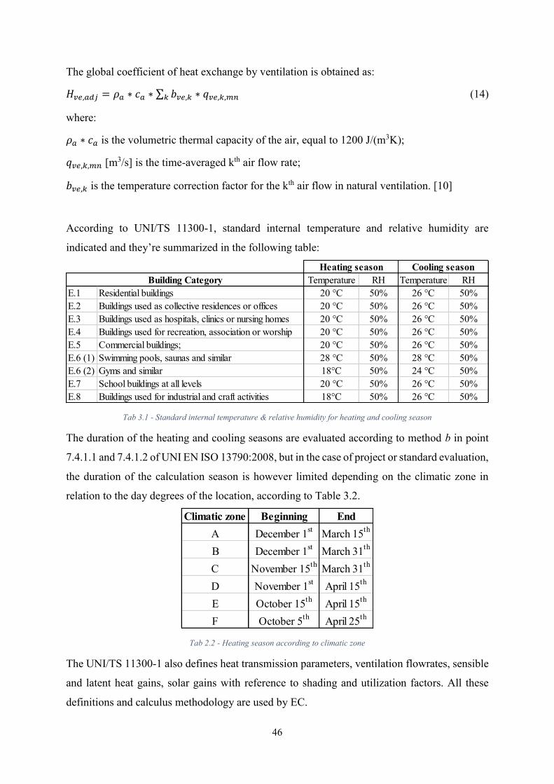
46
The global coefficient of heat exchange by ventilation is obtained as:
𝐻𝑣𝑒,𝑎𝑑𝑗 = 𝜌𝑎 ∗ 𝑐𝑎 ∗ ∑ 𝑏𝑣𝑒,𝑘 ∗ 𝑞𝑣𝑒,𝑘,𝑚𝑛𝑘 (14)
where:
𝜌𝑎 ∗ 𝑐𝑎 is the volumetric thermal capacity of the air, equal to 1200 J/(m3K);
𝑞𝑣𝑒,𝑘,𝑚𝑛 [m3/s] is the time-averaged kth air flow rate;
𝑏𝑣𝑒,𝑘 is the temperature correction factor for the kth air flow in natural ventilation. [10]
According to UNI/TS 11300-1, standard internal temperature and relative humidity are
indicated and they’re summarized in the following table:
Tab 3.1 - Standard internal temperature & relative humidity for heating and cooling season
The duration of the heating and cooling seasons are evaluated according to method b in point
7.4.1.1 and 7.4.1.2 of UNI EN ISO 13790:2008, but in the case of project or standard evaluation,
the duration of the calculation season is however limited depending on the climatic zone in
relation to the day degrees of the location, according to Table 3.2.
Tab 2.2 - Heating season according to climatic zone
The UNI/TS 11300-1 also defines heat transmission parameters, ventilation flowrates, sensible
and latent heat gains, solar gains with reference to shading and utilization factors. All these
definitions and calculus methodology are used by EC.
Temperature RH Temperature RH
E.1 Residential buildings 20 °C 50% 26 °C 50%
E.2 Buildings used as collective residences or offices 20 °C 50% 26 °C 50%
E.3 Buildings used as hospitals, clinics or nursing homes 20 °C 50% 26 °C 50%
E.4 Buildings used for recreation, association or worship 20 °C 50% 26 °C 50%
E.5 Commercial buildings; 20 °C 50% 26 °C 50%
E.6 (1) Swimming pools, saunas and similar 28 °C 50% 28 °C 50%
E.6 (2) Gyms and similar 18°C 50% 24 °C 50%
E.7 School buildings at all levels 20 °C 50% 26 °C 50%
E.8 Buildings used for industrial and craft activities 18°C 50% 26 °C 50%
Building Category
Heating season Cooling season
Climatic zone Beginning End
A December 1st
March 15th
B December 1st
March 31th
C November 15th
March 31th
D November 1st
April 15th
E October 15th
April 15th
F October 5th
April 25th

47
UNI/TS 11300-2 "Evaluation of primary energy need and of system efficiencies for space
heating, domestic hot water production, ventilation and lighting for non-residential buildings"
for the calculation of heating system efficiencies, electrical needs for ventilation and lighting,
and for the determination of DHW consumption.
The technical specification provides data and methods for the calculation of the efficiencies and
losses of the generation subsystems fuelled by liquid or gaseous fossil fuels. It applies to newly
designed, renovated or existing systems for heating, for mixed use or combined for both heating
and DHW production, for production of hot water for hygienic-sanitary uses only, for
ventilation systems, for ventilation systems combined with space heating, for lighting systems
in non-residential buildings. UNI/TS 11300-2 provides the definition of generation and
utilization systems and subsystems for both air conditioning and ventilation.
Figure 3.3- The energy balance of the building for heating – UNI/TS 11300-2 [19]
For each subsystem Y dedicated to service X, the following quantities need to be determined:
- the required input energy demand of subsystem 𝑄𝑋,𝑌,𝑖𝑛;
- the total auxiliary energy required 𝐸𝑋,𝑌,𝑎𝑢𝑥;
- losses 𝑄𝑋,𝑌,𝑙;
- the recovered losses 𝑄𝑋,𝑌,𝑙𝑟ℎ.
These estimations are made on the base of:
- useful energy to be provided at the output 𝑄𝑜𝑢𝑡,𝑋;
48
- characteristics of the subsystem and operating conditions of the installation.
The following thermal balance equation applies for each subsystem:
𝑄𝑋,𝑌,𝑖𝑛 = 𝑄𝑋,𝑌,𝑜𝑢𝑡 + 𝑄𝑋,𝑌,𝑙 − (𝑄𝑋,𝑌,𝑙𝑟ℎ + 𝑄𝑋,𝑌,𝑙,𝑟ℎ,𝑍 + 𝑄𝑋,𝑌,𝑎𝑢𝑥,𝑟ℎ) [MWh] (15)
where:
𝑄𝑋,𝑌,𝑖𝑛 is the thermal energy input to subsystem Y dedicated to service X;
𝑄𝑋,𝑌,𝑜𝑢𝑡 is the thermal energy output to subsystem Y dedicated to service X;
𝑄𝑋,𝑌,𝑙 is the thermal energy loss in subsystem Y dedicated to service X;
𝑄𝑋,𝑌,𝑙𝑟ℎ,𝑋 represents the thermal energy losses recovered in subsystem Y and charged in X;
𝑄𝑋,𝑌,𝑙,𝑛𝑟ℎ represents the thermal energy losses not recovered in subsystem Y.
𝑄𝑋,𝑌,𝑎𝑢𝑥,𝑟ℎ,𝑋 is the thermal energy recovered from the electrical energy dissipated in the form
of heat from the auxiliaries of subsystem Y;
𝑄𝑋,𝑌,𝑙,𝑟ℎ,𝑍 represents any recovered losses to be charged to the generic service Z.
The average efficiency of the subsystems can be derived from the thermal balance equation of
a subsystem and by taking into account the needs of auxiliaries.
For the generic subsystem Y, the efficiency in terms of primary energy in the considered
calculation period is equal to:
𝜂𝑌,𝑃 =∑ 𝑄𝑌,𝑜𝑢𝑡,𝑖𝑖
∑ 𝐸𝑌,𝑖𝑛,𝑗∗𝑓𝑃,𝑗+∑ 𝐸𝑌,𝑎𝑢𝑥,𝑗∗𝑓𝑃,𝑒𝑙𝑗𝑗 (16)
where:
𝑄𝑌,𝑜𝑢𝑡,𝑖 represents the energy in the form of the ith energy vector outgoing or produced by
subsystem Y;
𝐸𝑌,𝑖𝑛,𝑗 represents the energy in the form of the jth energy vector ingoing or supplied to
subsystem Y;
𝐸𝑌,𝑎𝑢𝑥,𝑗 is the electrical energy requirement of the auxiliaries of subsystem Y;
𝑓𝑃,𝑗 is the conversion factor into primary energy; it depends on the energy carrier that is used;
𝑓𝑃,𝑒𝑙 is the conversion factor of electrical energy into primary energy.
The formula (13) is of a general nature and expresses the efficiency as the ratio between
produced or outgoing energy and the ingoing or supplied energy to the subsystem expressed in
primary energy.
The efficiency of each subsystem can be calculated on a monthly basis, considering the input
and output needs of the subsystem, together with the needs of auxiliaries, for each month, or on

49
a seasonal basis, meaning relatively to the entire activation period of the heating season, taking
into account the sum of the monthly needs over the activation period.
If the average efficiency is required for more than one calculation interval, this is given by the
following formulas referring respectively to heating and domestic hot water services:
𝜂𝐻 =∑ 𝑄𝐻,𝑛𝑑,𝑖𝑖
∑ 𝐸𝑝,𝐻𝑗 (17)
𝜂𝑊 =∑ 𝑄𝑊,𝑛𝑑,𝑖𝑖
∑ 𝐸𝑝,𝑊𝑗 (18)
The same formulas can be applied to the useful thermal energy and to primary energy amounts
of the individual zones. [11]
For each kind of subsystem (emission, regulation, distribution, storage, generation) for both
HVAC and DHW systems, thermal energy needs and losses are defined, highlighting critical
situations and using outlines to show possible systems’ configurations. Attention is paid also to
the electrical energy needs of the auxiliaries of these subsystems, that may be determined or
when designing the installation or with measures on the installation or by calculation methods
based on benchmarks.
UNI/TS 11300-3 "Evaluation of primary energy and system efficiencies for space cooling" for
the calculation of the efficiencies of the cooling system of buildings or of single building units.
The technical specification applies only to fixed summer air-conditioning systems with
electrically-operated or absorption-operated refrigeration units. It applies to newly designed,
refurbished or existing systems:
- for cooling only;
- for summer air conditioning.
The method for determining the primary energy need for the summer cooling of a building is
specified. The calculation is divided into the following phases:
- determination of the ideal cooling demand 𝑄𝐶,𝑛𝑑, according to UNI/TS 11300-1:2008;
- calculation of emission losses, regulation, distribution and accumulation of the plant and
calculation of any recovered energy;
- calculation of air treatment demand 𝑄𝑉;
- calculation of the electrical energy needs for auxiliaries of air treatment 𝑄𝑎𝑢𝑥
- calculation of the average monthly performance coefficient 𝜂𝑚𝑚 of the refrigeration
machines, through the evaluation of reference performance data provided by the
manufacturers;

50
- Calculation of the primary energy demand for summer air conditioning 𝑄𝐶,𝑃.
The primary energy need for summer cooling is calculated using the following formula:
𝑄𝐶,𝑃 = ∑ 𝑄𝑎𝑢𝑥,𝑘 ∗ 𝑓𝑝,𝑒𝑙 + ∑ [∑𝑄𝐶𝑟,𝑘,𝑥+𝑄𝑣,𝑘,𝑥
𝜂𝑚𝑚,𝑘,𝑥𝑥 ] 𝑓𝑝,𝑥𝑘𝑘 [kWh] (19)
where:
𝑄𝑎𝑢𝑥 [kWh] is the electricity requirement for auxiliary air conditioning systems;
𝑄𝐶𝑟 [kWh] is the actual need for cooling;
𝑄𝑣 [kWh] is the need for air treatments;
𝜂𝑚𝑚 is the average monthly performance coefficient of the refrigeration energy production
system;
𝑓𝑝,𝑒𝑙 is the conversion factor from electrical energy to primary energy, determined according to
UNI/TS 11300-2:2008;
𝑓𝑝,𝑥 is the conversion factor to primary energy of the energy vector used by the generator;
𝑘 is the kth month of the summer cooling season, determined according to UNI/TS 11300-1;
𝑥 is the index that indicates the different sources of energy input.
The global seasonal average efficiency of the building-plant system is therefore determined as:
𝜂𝑔𝑙𝑜 =∑ (𝑄𝐶,𝑛𝑑,𝑘+𝑄𝑣)𝑘
𝑄𝐶,𝑃 (20)
where the different terms have the previously defined meanings.
The actual cooling demand 𝑄𝐶𝑟,𝑘 for each month of the cooling season is evaluated as follows:
𝑄𝐶𝑟,𝑘 = 𝑄𝐶,𝑛𝑑,𝑘 + 𝑄𝑙,𝑒,𝑘 + 𝑄𝑙,𝑟𝑔,𝑘 + 𝑄𝑙,𝑑,𝑘 + 𝑄𝑙,𝑑,𝑠,𝑘 − 𝑄𝑟𝑟,𝑘 [kWh] (21)
where for the kth month:
𝑄𝐶,𝑛𝑑,𝑘 [kWh] is the ideal need of the building;
𝑄𝑙,𝑒,𝑘 [kWh] represents the total emission losses;
𝑄𝑙,𝑟𝑔,𝑘 [kWh] represents the total control losses;
𝑄𝑙,𝑑,𝑘 [kWh] represents the total distribution losses;
𝑄𝑙,𝑑,𝑠,𝑘 [kWh] represents the total losses of the inertial storage tanks;
𝑄𝑟𝑟,𝑘 [kWh] is the thermal energy recovered.
UNI/TS 11300-3 then provides all the equations to calculate all these terms, the corrective
coefficients to adapt calculations to different situations and the energy performance coefficients
of refrigeration systems. [12]
51
UNI/TS 11300-4 "Renewable energy and other generation systems for space heating and
domestic hot water production" for the calculation of primary energy demands for space heating
and domestic hot water production where there are generation subsystems that provide useful
thermal energy from renewable energies or by generation methods different from flame burning
fossil fuels (covered by UNI/TS 11300-2).
Among all the renewable energy sources, solar thermal, biofuels, air, geothermal and hydraulic
sources in the case of heat pumps for the share considered renewable are considered for useful
thermal energy production, and photovoltaic solar for electric energy production.
For what concerns generation methods different from flame burning fossil fuels, heat pumps,
cogeneration and district heating are considered. (Regarding district heating, only thermal
energy delivered to the plant and the equivalent primary energy are considered.)
This technical specification provides the evaluation of primary energy needs, primary energy
contributions from each energy vector, CO2 production from each energy vector and from the
all system. Data for these evaluations must be indicated separately for energy vector and for
type of service on monthly and annual basis.
For all these energy sources, calculation methodologies for the estimation of their performance
parameters and of the amount of energy produced by each of them are provided. [13]
UNI/TS 11300-5 "Calculation of primary energy and the amount of energy from renewable
sources". This standard specifies:
- the boundaries of the evaluation of the building, explaining which are the energy sources
that can be considered inside or outside the building;
- renewable and non-renewable energy sources;
- the way in which performance indicators are defined;
- the services included in the calculation of the energy requirements of the building;
- the formulas for the conversion into primary energy of the contributions of energy delivered
to the building by energy carriers;
- the way in which energy contributions are allocated to individual services;
- the method for evaluating the share of energy from renewable sources, in accordance with
the requirements of Legislative Decree 28 of 3 March 2011 (Annex 3).
Recommendation CTI 14 "Energy performance of buildings - Determination of energy
performance for building classification".

52
3.1.3 Space cooling power calculation by EC706
The program EC706 – Space cooling power, thanks to the loading of input data through EC700
- Calculation of energy performance of buildings, allows to perform the calculation of cooling
power, according to the Carrier method. In particular, the program allows the calculation of the
thermal loads for radiation, transmission, ventilation and internal loads.
The purpose of EC706 is to provide the user with a detailed assessment of the global summer
loads of the rooms and zones.
As already mentioned, the calculation method adopted by the program is represented by the
Carrier method. It allows the separate evaluation of
- thermal loads by solar radiation through the windowed components;
- thermal loads by transmission through the opaque or windowed components;
- thermal loads by ventilation;
- internal thermal loads, resulting from the presence of people and electrical machinery.
The thermal loads due to solar radiation through the windowed components can be evaluated
by adopting or not the methodology relating to the "accumulation factors". The evaluation of
thermal loads by radiation also considers the shading factors, in addition to other specific
parameters of interest.
The thermal loads for transmission through opaque or windowed components are calculated by
determining the "equivalent temperature difference" between the internal and external
environment, a differential evaluated according to the Carrier method depending on the time of
day and month.
The ventilation loads are evaluated on the basis of the air exchange rates set by the user and
according to the thermo-hygrometric conditions of the internal and external air, the latter
evaluated according to the time and month.
The internal loads for people and electrical machinery are evaluated by means of specific input
data requested from the user relating to specific thermal loads.
All the above calculation results can be evaluated for six time-bands from 8 a.m. to 6 p.m., for
all the relevant months or only for the "peak month" of the location under examination.
The analyses are generally carried out according to the reference location set by the user, the
exposure of the components analysed, their type and their specific characteristics.
53
3.2 DesignBuilder
DesignBuilder was born from a European project and is proposed as a high-quality tool for
serious and reliable energy analysis of buildings. It consists of a modelling Graphical User
Interface (GUI) connected to several modules, each providing a particular functionality. The
precision of the calculations is guaranteed by the use of EnergyPlus© and the three-dimensional
graphic interface dedicated only to the representation of the building make it a suitable working
tool for by architects, construction engineers, thermal engineers and students
DesignBuilder is a user-friendly modelling environment that provides a range of building
performance data such as: energy consumption, carbon emissions, comfort conditions, daylight
illuminance, maximum summertime temperatures and HVAC component sizes.
In particular, it allows to:
- evaluate a series of types of facades to quantify the effects of overheating, energy use and
visual impact of the building;
- evaluate the optimal use of natural light and model lighting control systems to calculate the
savings in electric lighting;
- display solar shadows at any time of year;
- make thermal simulations of naturally ventilated buildings;
- calculate the power of space heating and cooling systems in a very short time.
- make dynamic calculations of thermal and cooling loads (ASHRAE Test certified 140)
- simulate fuel and electricity consumption for any period of time;
- connect to world climatic databases;
- calculate CO2 production;
- calculate the real temperatures in the non-conditioned areas of the building.
DesignBuilder can operate with 3D CAD systems using gbXML standards, even if there are
limitations for inputting complex geometry (e.g. geometries defined through smooth functions).
3.2.1 SketchUp & OpenStudio Plug-in
Even if DesignBuilder has its own GUI, it can operate with 3D CAD coming from other
modelling software, as long as they’re in gbXML format. SketchUp allows to create 3D models
of buildings and, thanks to OpenStudio plug-in, to export them in the necessary format to be
opened in DesignBuilder and that’s what was done in this case.
SketchUp is a 3D modelling computer program for a wide range of drawing applications,
owned by Trimble Inc., that is available as a web-based application, SketchUp Free, as a
freeware version, SketchUp Make, and as a paid version with additional functionality (such as

54
importation of 2D CAD), SketchUp Pro. For this work, SketchUp Make was used to create the
3D model of the building.
OpenStudio is a cross-platform collection of software tools to support whole building energy
modelling using EnergyPlus and advanced daylight analysis using Radiance.
The graphical applications include the OpenStudio SketchUp Plug-in, which is an extension to
SketchUp 3D modelling tool that allows users to quickly create geometry needed for
EnergyPlus. Thanks to OpenStudio Plug-in it’s possible to define the thermal zones composing
the building, that DesignBuilder recognizes, and to export the 3D model as gbXML file in order
to be opened in DesignBuilder environment.
3.2.2 The simulation engine: EnergyPlus
The two main components of the building energy simulation model are the building fabric and
content (walls, floors, ceilings, occupants and equipment) and the plant components (HAVC
equipment and other environmental control systems). Due to the complexity of a building
model, computer simulations can analyse the effects of different ECMs (Energy Conservation
Measures) and their complex interactions more efficiently, comprehensively and accurately that
any other available method. DesignBuilder is used with EnergyPlus as the simulation engine in
this case.
EnergyPlus is the U.S. Departments of Energy’s dynamic building energy simulation engine
for modelling building, heating, cooling, lighting, ventilating and other energy flows. The
program was developed during the nineties and is an amalgamation of the BLAST and DOE-2
simulation engines. Apart from energy use, the program can be used for load calculations and
to model natural ventilation, photovoltaic systems, thermal comfort, water use, green roofs and
other ECMs. EnergyPlus is integrated within DesignBuilder’s environment which allows the
user to carry out complete simulations without leaving the interface. Simulation results can be
effectively displayed and analysed in a comprehensive manner. DesignBuilder has quality
control procedures which assure the accuracy of the results in comparison the stand-alone
EnergyPlus engine. As EnergyPlus, it has been tested under the comparative Standard Method
BESTEST/ASHARE STD 140. [14]
EnergyPlus solves the heat balance calculation with respect to the air node considering
separately the convective and the radiative exchanges. The air node balance is expressed as
function of the convective thermal exchanges:
𝛷𝑐 + 𝛷𝑣 + 𝛷𝑖 + 𝛷ℎ = 𝐶𝑎𝑖𝑑𝑇𝑖
𝑑𝜏 [W] (21)
where

55
𝛷𝑐 is the convection heat flow between air and adjacent surfaces;
𝛷𝑣 is the infiltration and ventilation sensible thermal power;
𝛷𝑖 is the convective thermal power from internal sources;
𝛷ℎ is the convective thermal power extracted/added from HVAC plant;
𝑇𝑖 is the indoor temperature;
𝜏 is the time;
𝐶𝑎𝑖 is the indoor air thermal capacity.
The surface convective exchange 𝜑𝑐,𝑖 is determined solving the surface heat balance, per unit
of surface, for the internal side. For each j-surface:
𝜑𝑐,𝑖,𝑗 + 𝜑𝑟,𝑖,𝑗 + 𝜑𝑠𝑜𝑙,𝑖,𝑗 + 𝜑𝑐𝑑,𝑗 +𝛷𝑖,𝑟+𝛷ℎ,𝑟
∑ 𝐴𝑘𝑁𝑘=1
= 0 (20)
where
𝜑𝑖,𝑟 [W] is the radiation heat flux from internal sources;
𝜑ℎ,𝑟 [W] is the radiation heat flux from heating plant;
𝐴𝑘 [m2] is the area of the kth element of the environment.
𝜑𝑟,𝑖 [W/m2] is the specific longwave radiation heat flux exchanged with other internal surfaces;
𝜑𝑠𝑜𝑙,𝑖 [W/m2] is the specific absorbed radiation shortwave heat flux;
𝜑𝑐𝑑,𝑖 [W/m2] is the specific conduction heat flux at the internal surface;
The external boundary conditions are defined by the balance equation:
𝜑𝑟,𝑜,𝑗 + 𝜑𝑠𝑜𝑙,𝑜,𝑗 + 𝜑𝑐,𝑜,𝑗 + 𝜑𝑐𝑑,𝑜,𝑗 = 0 (22)
where
𝜑𝑟,𝑜 [W/m2] is the specific longwave radiation heat flux exchanged with outdoor surfaces;
𝜑𝑠𝑜𝑙,𝑜 [W/m2] is the specific absorbed radiation shortwave heat flux;
𝜑𝑐𝑑,𝑜 [W/m2] is the specific conduction heat flux at the external surface;
𝜑𝑐,𝑜 [W/m2] is the specific convection heat flux with outdoor air.
In particular, the external long wave radiation is calculated considering the exchanges with the
external surrounding elements (ground, other buildings, sky vault). [15]
3.2.3 Compliance with requirements
DesignBuilder v5 complies with the requirements of ANSI/ASHRAE/ACCA Standard 183-
2007, Peak Cooling and Heating Load Calculations in Buildings Except Low-Rise Residential
Buildings. In particular, sections 5 to 10 from Standard 183-2007 are considered and for almost
all of them, the compliance with the requirements is achieved by Design Builder. [16]
Figure 3.4 - Surface heat balance

56
3.3 THERM 7.6
THERM is a state-of-the-art computer program developed at Lawrence Berkeley National
Laboratory (LBNL) to be used by building component manufacturers, engineers, educators,
students, architects, and others interested in heat transfer.
THERM allows to model two-dimensional heat-transfer effects in building components such
as windows, walls, foundations, roofs, doors and other products where thermal bridges are of
concern. Its heat-transfer analysis allows the user to evaluate a product’s energy efficiency and
local temperature patterns, which may relate directly to problems with condensation, moisture
damage and structural integrity. [17]
THERM’s two-dimensional conduction heat-transfer analysis is based on the finite-element
method, which can model the complicated geometries of building products. The program’s
graphic interface allows to draw cross sections of products or components to be analysed,
tracing imported files in DXF format. Each cross section is represented by a combination of
polygons. For each polygon the material properties are defined and the environmental
conditions to which the component is exposed are introduced by defining the boundary
conditions surrounding the cross section. This method requires that the cross section be divided
into a mesh made up of non-overlapping elements. This process is performed automatically by
THERM using the Finite Quadtree method. Once the user has defined the cross-section’s
geometry, material properties and boundary conditions, THERM meshes the cross section,
performs the heat-transfer analysis, runs an error estimation, refines the mesh if necessary, and
returns the converged solution. [17]
Figure 3.5 - Therm’s flow
The results from THERM's finite-element analysis can be viewed as:
▪ U-factors,
▪ isotherms,
▪ colour-flooded isotherms,
▪ heat-flux vector plots,
▪ colour-flooded lines of constant flux,
▪ temperatures

57
4. Methodology
In this chapter the procedure that has been followed to achieve the results is discussed. Initially,
the diagrams of the different floors of the building are shown, then the simplifications
implemented to create the models with Edilclima and DesignBuilder are described, explaining
all the steps that led to the development of these models; subsequently, the results given by the
two softwares are examined and confronted and finally a comparison between two conditioning
strategies for the ground floor is carried out.
4.1 Building’s design diagrams and front views
As mentioned in chapter 2, the building is made up of three main floors and a basement. The
building is characterized by large open spaces that allows the interconnection between the
different working areas, and is designed to have harmonized shapes and plenty of lights, thanks
to a large number of windows. The following pictures show the design diagrams of the four
floors of the future Innovation Square centre, the front views of each side, and two sections of
the building as it’s meant to become.
Figure 4.1 - Basement’s diagram

58
The basement is occupied by three spaces to be conditioned, which are the changing rooms for
workers (“spogliatoio lavoratori” and “spogliatoi cucina”) and a stock (“magazzino 3”). The
other rooms are dedicated to storage and to technical machinery: in this analysis they’ll be
considered as non-conditioned. The basement is 2.50 meters high and is underground for 2.10
meters. The rest of the underground area includes a car park.
In this map, as in the following ones, the pink dashed line represents the border with the adjacent
property. The orientation of the building is given by the compass in the bottom right angle of
the figure, therefore the upper façade faces North, the right façade East, the bottom one South
and the left one West, even if with a deviation of 31°.
The building can be accessed by two main entrances: one located on the East side and one on
the West side (mainly dedicated to employees and janitor).
Figure 4.2 - Ground floor's diagram
The ground floor is the largest of the building and the one that hosts spaces belonging to
different DPR 412/93 categories. In fact, it includes the restoration area (E.4) and the janitor’s
house (E.1), besides the manufacturing offices and laboratories (E.8). As previously described,
this large environment is characterised by different heights depending on the use destination

59
and on the position of the rooms. The central part, with that dynamic shape, is the one that is
going to be built from scratch since in the original structure the large central square was left
“empty” and completely opened to the rest of the building. In this central structure, meeting
rooms are located at ground level (which is 0.9 meters above the terrain height). The restoration
area is located on the North side and, as it can be seen in figure 4.6, is characterized by a glass
wall. Its main part is opened to the central square and to the first floor, since it’s 5.5 meters
high. The rest of the ground floor is occupied by meeting and storage rooms and laboratories.
The storage room (“magazzino PT) is 3.56 meters high and its walls stand underground for 0.50
meters.
Figure 4.3 - First floor's diagram
The first and second floors (represented respectively in figures 4.3 and 4.4) are characterized
by decreasing floor areas and they both face the open central square. Both floors are occupied
by manufacturing offices and restrooms and present large corridors that are going to become
offices and so be closed by glass partitions at a later stage. Offices are mainly delimited by glass
partitions in order to give the sense of sharing and collaboration sought by the client.
The first floor has an average internal height of 2.50 m, except for the central part, which is
occupied by manufacturing offices having 2.70 meters high walls. The second floor is a little
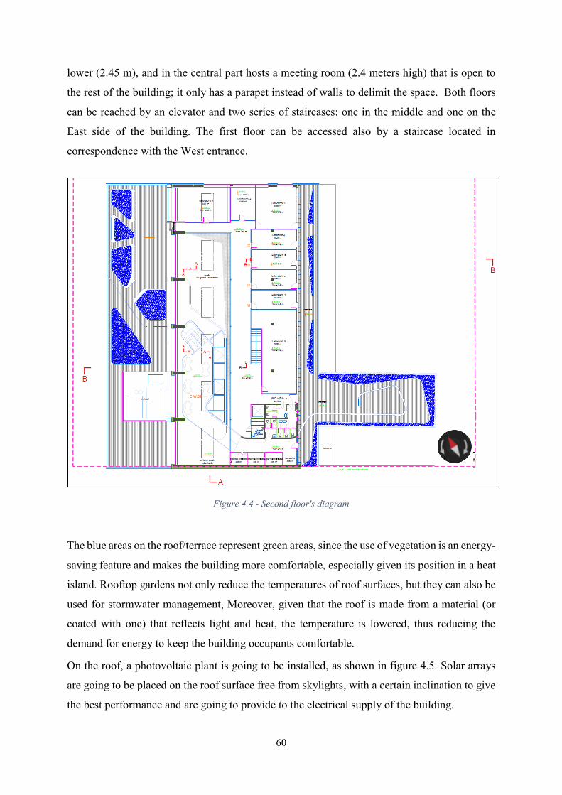
60
lower (2.45 m), and in the central part hosts a meeting room (2.4 meters high) that is open to
the rest of the building; it only has a parapet instead of walls to delimit the space. Both floors
can be reached by an elevator and two series of staircases: one in the middle and one on the
East side of the building. The first floor can be accessed also by a staircase located in
correspondence with the West entrance.
Figure 4.4 - Second floor's diagram
The blue areas on the roof/terrace represent green areas, since the use of vegetation is an energy-
saving feature and makes the building more comfortable, especially given its position in a heat
island. Rooftop gardens not only reduce the temperatures of roof surfaces, but they can also be
used for stormwater management, Moreover, given that the roof is made from a material (or
coated with one) that reflects light and heat, the temperature is lowered, thus reducing the
demand for energy to keep the building occupants comfortable.
On the roof, a photovoltaic plant is going to be installed, as shown in figure 4.5. Solar arrays
are going to be placed on the roof surface free from skylights, with a certain inclination to give
the best performance and are going to provide to the electrical supply of the building.

61
Figure 4.5 - Roof's representation
The following figures show the front views of the four facades of the building.
Figure 4.6 - North front view
Figure 4.7 - East front view

62
Figure 4.8 - South front view
The small windows on the South façade are kept from the original structure to give a sense of
continuity with the previous industrial site. The wall of the adjacent property is 4.45 meters
high and makes shadow over the building.
Figure 4.9 - West front view
4.2 Simplifications to model the building
As shown in the previous paragraph, the design project of the Innovation Square Center is
ambitious and includes a lot of volumes of different shapes and height. Due to the complexity
of its interior, but not only for this reason, some simplifications are made to model the building
in Ediclima and DesignBuilder. One of them involves the sloped concrete structure in the North
façade that both the original and the renovated building present. That element has not been
represented in the model in order not to add useless surfaces and to calculate easily the internal
volumes of the zones. The other simplifications are listed below.
4.2.1 Absence of the central structure
Even if the structure to be built in the middle of the building will be its distinctive mark, the
original aspect of the Innovation Square Center, this work is not taking it into consideration.
The removal of this part from the analysis is made as a result of two observations:

63
- In the preliminary document to be exposed to the competent authority this part is not
included and all the energy evaluations are made on this “temporary” building;
- The large number of curved surfaces makes it difficult to create a 3D model of the building
to be supported by DesignBuilder.
The following figures show the sections and diagrams of the “simplified building” that have
been used to create the model that has been analysed by the two softwares.
Figure 4.10 - Ground floor simplified diagram
In addition to the elimination of the central structure, all the other curved surfaces have been
approximated with flat ones. For instance, the curved lines that delimitate the prototype
preparation area (see figure 4.10), in the 3D model have been drawn with a small number of
segments, so that the shape is partially kept, but the surfaces that the software considers are
reduced.

64
Figure 4.11 - First floor simplified diagram
Figure 4.12 - Second floor simplified diagram

65
Figure 4.13 - Section A-A of the simplified model
Figure 4.14 - Section B-B of the simplified model
These two sections give the idea of the aperture of the central space on the rest of the building.
4.2.2 Internal partitions
As previously mentioned and shown, the internal partitions are of different kind: the ones that
enclose offices are glazed, some include concrete elements and the remaining ones are made of
bricks. In Edilclima, internal partitions are generally not defined since they separate equally
conditioned rooms, so there is no need to differentiate partitions. Only the storage room is
conditioned differently from the rest of the building, and the elevator shaft is not conditioned:
partitions of these spaces are both brick walls and need to be defined. DesignBuilder, instead,
automatically recognizes internal partitions. In this case, all internal partitions are defined in
the same way, as brick walls. This is done both to reduce input data for the program and to
make conservative evaluations.
4.2.3 Orientation’s definition
The building’s orientation is 31° with respect to the North direction. This angle is considered
in DesignBuilder’s model, while it isn’t in Edilclima. The façades are oriented to the cardinal
directions, without specifying that they present an offset from them.

66
4.3 Definition of building’s components
Since the project involves a renovation, some of the components of the design building need to
be substituted for aesthetic, structural and normative reasons, like doors, windows and roof.
Others are adjusted to meet normative requirements and resistance characteristics, and that’s
the case of walls, ceilings and floors. In the following pages, the stratigraphy of walls, floors,
ceilings and roof are illustrated. In the tables below, R is the thermal transmittance, V.M. stands
for Volumetric Mass, T.C. is the Thermal Capacity, R.V. is the factor of resistance to vapour
diffusion in dry garments.
For transparent components (windows and glazed doors), only transmittances and shading
factors are displayed. In fact, windows differ only for their shape, but not in terms of their
thermal parameters, which is the main aspect to be considered.
External wall
External walls keep the same structure as they had in the ‘60s, but they’re insulated as much as
it’s necessary to reach the transmittance requirement as in the DM 26.06.2015. Basically,
external walls are cavity walls with a layer of insulation materials added on the outside part.
Table 4.1 and Table 4.2 show their stratigraphy and properties evaluated from Edilclima.
Tab 4.1 - External wall’s layer
Tab 4.2 - External wall’s stratigraphy and properties according to Edilclima
N. Layer Description s [mm] λ
[W/mK]
R
[m2K/W]
V.M
[m3/kg]
T.C.
[kJ/kgK] R.V
- Internal surface resistance - - 0,130 - - -
1 Sand plaster 10 1,000 0,010 1800 1,00 10
2 Internal brickwork (hum. 0.5%) 80 0,300 0,267 800 1,00 7
3 Non-ventilated air gap Av<500 mm²/m 200 1,111 0,180 - - -
4 External brickwork (hum. 1.5%) 120 0,410 0,293 800 1,00 7
5 Expanded Sintered Polystyrene (EPS 150) 120 0,034 3,529 20 1,45 60
6 Plastic plaster 10 0,300 0,033 1300 0,84 30
- External surface resistance - - 0,071 - - -
Thermal transmittance 0,222 W/m2K
Thickness 540 mm
Permeance 22,198 10-12kg/sm2Pa
Surface mass (including plasters) 193 kg/m2
Surface mass (excluding plasters) 162 kg/m2
Periodic thermal transmittance 0,039 W/m2K

67
Internal wall
As previously mentioned, internal walls are all defined as opaque and made of bricks, as shown
in the following tables.
N. Layer Description s
[mm]
λ
[W/mK]
R
[m2K/W]
V.M
[m3/kg]
T.C.
[kJ/kgK] R.V
- Internal surface resistance - - 0,130 - - -
1 Sand plaster 10 1,000 0,010 1800 1,00 10
2 Alveolated brick masonry 120 0,320 0,375 870 1,00 5
3 Sand plaster 10 1,000 0,010 1800 1,00 10
- External surface resistance - - 0,130 - - -
Tab 4.3 - Internal wall’s layers
Tab 4.4 - Internal wall’s stratigraphy and properties according to Edilclima
Ground floor
Even the ground floor is the old manufactured one, but a layer of insulation has been added so
that it’s compliant with the requirement (U≤0.26 W/m2K).
N. Layer Description s
[mm]
λ
[W/mK]
R
[m2K/W]
V.M
[m3/kg]
T.C.
[kJ/kgK] R.V
- Internal surface resistance - - 0,170 - - -
1 Plastic floor 20 0,250 0,080 1700 1,40 104
2 Expanded Sintered Polystyrene (EPS 150) 60 0,034 1,765 20 1,45 60
3 Concrete distribution screed with net 30 1,490 0,020 2200 0,88 70
4 Concrete 300 1,060 0,283 1900 1,00 96
- External surface resistance - - 0,040 - - -
Tab 4.5 - Ground floor's layers
Tab 4.6 - Ground floor’s stratigraphy and properties according to Ediclima
Thermal transmittance 1,527 W/m2K
Thickness 140 mm
Permeance 250,00 10-12kg/sm2Pa
Surface mass (including plasters) 140 kg/m2
Surface mass (excluding plasters) 104 kg/m2
Periodic thermal transmittance 1,096 W/m2K
Transmittance through terrain 0,253 W/m2K
Thickness 410 mm
Permeance 0,853 10-12kg/sm2Pa
Surface mass 671 kg/m2
Periodic thermal transmittance 0,041 W/m2K
Thermal conductivity of the terrain 2,00 W/mK
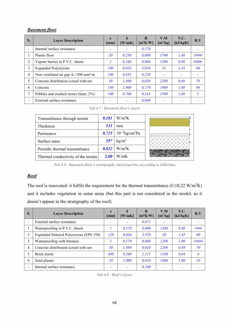
68
Basement floor
N. Layer Description s
[mm]
λ
[W/mK]
R
[m2K/W]
V.M
[m3/kg]
T.C.
[kJ/kgK] R.V
- Internal surface resistance - - 0,170 - - -
1 Plastic floor 20 0,250 0,080 1700 1,40 10000
2 Vapour barrier in P.V.C. sheets 1 0,160 0,006 1390 0,90 50000
3 Expanded Polystyrene 100 0,033 3,030 35 1,45 60
4 Non-ventilated air gap Av<500 mm²/m 100 0,455 0,220 - - -
5 Concrete distribution screed with net 30 1,490 0,020 2200 0,88 70
6 Concrete 180 1,060 0,170 1900 1,00 96
7 Pebbles and crushed stones (hum. 2%) 100 0,700 0,143 1500 1,00 5
- External surface resistance - - 0,040 - - -
Tab 4.7 - Basement floor's layers
Tab 4.8 - Basement floor’s stratigraphy and properties according to Edilclima
Roof
The roof is renovated: it fulfils the requirement for the thermal transmittance (U≤0,22 W/m2K)
and it includes vegetation in some areas (but this part is not considered in the model, so it
doesn’t appear in the stratigraphy of the roof).
N. Layer Description s
[mm]
λ
[W/mK]
R
[m2K/W]
V.M
[m3/kg]
T.C.
[kJ/kgK] R.V
- External surface resistance - - 0,071 - - -
1 Waterproofing in P.V.C. sheets 1 0,170 0,006 1390 0,90 50000
2 Expanded Sintered Polystyrene (EPS 150) 120 0,034 3,529 20 1,45 60
3 Waterproofing with bitumen 1 0,170 0,006 1200 1,00 188000
4 Concrete distribution screed with net 30 1,490 0,020 2200 0,88 70
5 Brick insole 400 0,360 1,111 1100 0,84 6
6 Sand plaster 10 1,000 0,010 1800 1,00 10
- Internal surface resistance - - 0,100 - - -
Tab 4.9 - Roof’s layers
Transmittance through terrain 0,181 W/m2K
Thickness 531 mm
Permeance 0,725 10-12kg/sm2Pa
Surface mass 597 kg/m2
Periodic thermal transmittance 0,022 W/m2K
Thermal conductivity of the terrain 2,00 W/mK

69
Tab 4.10 - Roof’s stratigraphy and properties according to Edilclima
Inter-storey slab
It represents the element that separates one floor from the other: it’s the ceiling of the lower
space and the floor of the upper one, so it separates equally conditioned rooms (except for the
case in which it’s the ceiling of the storage room).
N. Layer Description s
[mm]
λ
[W/mK]
R
[m2K/W]
V.M
[m3/kg]
T.C.
[kJ/kgK] R.V
- External surface resistance - - 0,1 - - -
1 Ceramic tiles 10 1,000 0,010 2300 0,84 200
2 Substrate of lean cement 60 0,700 0,086 1600 0,88 20
3 Expanded Sintered Polystyrene (graphite) 100 0,031 3,226 20 1,45 60
4 Concrete 30 0,190 0,158 400 1,00 96
5 Predalles ceiling 240 0,857 0,280 1479 0,84 9
6 Gypsum insulating plaster 10 0,180 0,056 600 1,00 10
- Internal surface resistance - - 0,100 - - -
Tab 4.11 - Inter-storey slab’s layers
Tab 4.12 - Inter-storey slab's stratigraphy and properties according to Edilclima
Windows
Apart from the glazed wall on the North façade and the small windows on the South façade that
are preserved from the old ownership, all the windows are double-glazed with the same value
of thermal transmittance Uw = 1.2 W/m2K and are classified as permeability class 4, according
to UNI EN 12207. Data for the calculation of solar contributions, instead, change depending on
the orientation of the window. Table 4.13 summarizes all these characteristics.
Thermal transmittance 0,206 W/m2K
Thickness 562 mm
Permeance 0,801 10-12kg/sm2Pa
Surface mass (including plasters) 529 kg/m2
Surface mass (excluding plasters) 511 kg/m2
Periodic thermal transmittance 0,004 W/m2K
Thermal transmittance 0,249 W/m2K
Thickness 450 mm
Permeance 13,947 10-12kg/sm2Pa
Surface mass (including plasters) 494 kg/m2
Surface mass (excluding plasters) 488 kg/m2
Periodic thermal transmittance 0,029 W/m2K

70
Characteristics of the windows
Permeability Class Class 4 according to UNI EN 12207
Thermal transmittance Uw [W/m2K]
North double-glazed wall 1,090
South small single-glazed windows 5,315
All other windows (double-glazed) 1,200
Data for the calculation of solar contributions
Orientation NORTH EAST SOUTH WEST TOP
Emissivity ε 0,837 0,837 0,837 0,837 0,837
Winter curtains factor fc,winter 0,30 0,30 0,30 0,65 0,30
Summer curtains factor fc,summer 0,10 0,30 0,30 0,65 0,10
Solar transmittance factor ggl,n 0,70 0,70 0,85 0,85 0,85
Thermal resistance of closures [m2K/W] 0,15 0,00 0,00 0,00 0,15
f shut 0,6 0,6 0,6 0,6 0,6
Tab 4.13 - Characteristics of windows input e computed in Edilclima
4.4 Edilclima implementation
Edilclima uses the quasi-steady state method described in section 3.1.2 for energy calculations.
It calculates the heat balance over a sufficiently long enough time (month or year), which
enables to take dynamic effects into account by an empirically determined gain and/or loss
utilization factor. In the quasi-steady state methods, the dynamic effects are considered by
introducing correlation (utilization) factors. (If the time step is long enough, the U-value
approach is acceptable). The effect of thermal inertia in case of intermittent heating /cooling or
switch-off is considered separately.
In heating calculations, a utilization factor for internal and solar heat gains takes account for
the fact that only part of those gains is used to decrease the energy need for space heating, the
rest leads to an undesired increase of the internal temperature above the set-point.
In cooling calculations, a utilization factor for the transmission and ventilation heat transfer
takes account of the fact that only part of that heat transfer is utilised to decrease the cooling
needs. “Unused” transmission and ventilation heat transfers occur during periods or intervals
(e.g. nights) when they have no effect on the cooling needs taking place during other periods or
moments (e.g. days), but rather lead to temperatures below set-point.
In this section, the methodology that has been followed to create the model in Edilclima is
discussed, focusing on the main steps and on the results that have been obtained.
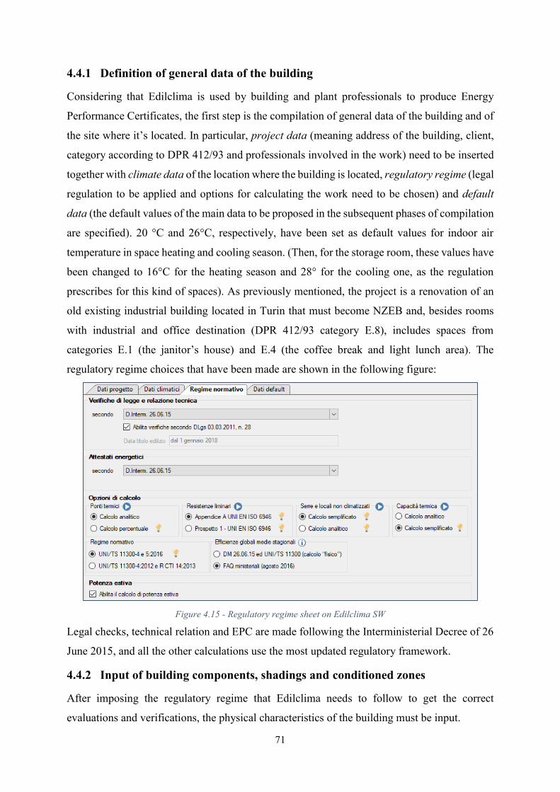
71
4.4.1 Definition of general data of the building
Considering that Edilclima is used by building and plant professionals to produce Energy
Performance Certificates, the first step is the compilation of general data of the building and of
the site where it’s located. In particular, project data (meaning address of the building, client,
category according to DPR 412/93 and professionals involved in the work) need to be inserted
together with climate data of the location where the building is located, regulatory regime (legal
regulation to be applied and options for calculating the work need to be chosen) and default
data (the default values of the main data to be proposed in the subsequent phases of compilation
are specified). 20 °C and 26°C, respectively, have been set as default values for indoor air
temperature in space heating and cooling season. (Then, for the storage room, these values have
been changed to 16°C for the heating season and 28° for the cooling one, as the regulation
prescribes for this kind of spaces). As previously mentioned, the project is a renovation of an
old existing industrial building located in Turin that must become NZEB and, besides rooms
with industrial and office destination (DPR 412/93 category E.8), includes spaces from
categories E.1 (the janitor’s house) and E.4 (the coffee break and light lunch area). The
regulatory regime choices that have been made are shown in the following figure:
Figure 4.15 - Regulatory regime sheet on Edilclima SW
Legal checks, technical relation and EPC are made following the Interministerial Decree of 26
June 2015, and all the other calculations use the most updated regulatory framework.
4.4.2 Input of building components, shadings and conditioned zones
After imposing the regulatory regime that Edilclima needs to follow to get the correct
evaluations and verifications, the physical characteristics of the building must be input.

72
Building components
At first, building components are defined. On EC they’re divided into categories: Walls, Floors,
Ceilings, Windowed components and Thermal Bridges. For Walls, Floors and Ceilings,
boundary conditions need to be specified, in particular they can separate the conditioned space
from the outdoor atmosphere, from the terrain, from a non-conditioned space or from differently
conditioned room. These specifications are necessary to allow EC to compute correctly the
thermal transmittance of the component, since the boundary conditions influences the surface
resistances. If a building component is present in more than one of the above-mentioned
situations, it must be defined as many times as the conditions in which it appears.
Building components are the ones introduced in section 4.3: their stratigraphies are the ones
previously shown, while the thermal transmittances indicated there are the ones referring to the
most widespread situation in terms of boundary conditions in the building. For these reasons,
in EC more components appear with respect to the ones presented above.
Their stratigraphies have been defined adding one layer at the time, selecting materials from
the library provided by the software, or creating them if not present.
Windows instead have been defined one by one, because even if they’re all of the same type
and so have the same physical properties (apart from the ones on the North and South sides),
they all have different dimensions. When defining windows, curtains and solar transmission
factors are also assigned. For this building, 67 windowed components have been defined.
Shadings
Shadings are defined in a different sheet and are then associated to the component on whom
they make shadow when defining the conditioned zones.
EC allows to input three kinds of
shadings: external obstacles, vertical
projections and horizontal projections. In
this case, only one shading is defined and
it’s the horizontal projection given by the
awning on the East façade: it’s an
extension of the first floor that provides
shade on the wall of the ground floor. Its
input on EC, called “Tettoia piano terra”
is shown in figure 4.16.
Figure 4.16 - Shading definition
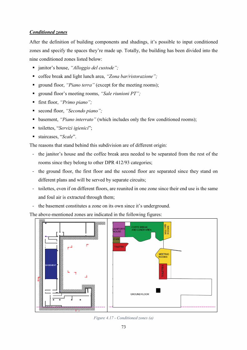
73
Conditioned zones
After the definition of building components and shadings, it’s possible to input conditioned
zones and specify the spaces they’re made up. Totally, the building has been divided into the
nine conditioned zones listed below:
▪ janitor’s house, “Alloggio del custode”;
▪ coffee break and light lunch area, “Zona bar/ristorazione”;
▪ ground floor, “Piano terra” (except for the meeting rooms);
▪ ground floor’s meeting rooms, “Sale riunioni PT”;
▪ first floor, “Primo piano”;
▪ second floor, “Secondo piano”;
▪ basement, “Piano interrato” (which includes only the few conditioned rooms);
▪ toilettes, “Servizi igienici”;
▪ staircases, “Scale”.
The reasons that stand behind this subdivision are of different origin:
- the janitor’s house and the coffee break area needed to be separated from the rest of the
rooms since they belong to other DPR 412/93 categories;
- the ground floor, the first floor and the second floor are separated since they stand on
different plans and will be served by separate circuits;
- toilettes, even if on different floors, are reunited in one zone since their end use is the same
and foul air is extracted through them;
- the basement constitutes a zone on its own since it’s underground.
The above-mentioned zones are indicated in the following figures:
Figure 4.17 - Conditioned zones (a)

74
Figure 4.18 - Conditioned zones (b)
Since in the regulatory regime sheet the simplified calculation method was chosen for
greenhouses and non-conditioned rooms, spaces such as the elevator shaft and the
unconditioned part of the basement haven’t been defined in the model. They are considered
when imposing the correct boundary conditions to the dispersing surfaces of the conditioned
spaces. In figures 4.17 and 4.18 the black squares represent the elevator shaft.
Inside each zone, spaces have been created, and for each of them tabular input was used to
define the dispersing surfaces: after measuring heights and areas from the CADs of diagrams
and front views of the building, gross dispersing surfaces have been manually inserted. Then,
for each space, net floor areas have been calculated and, by multiplying them for the
corresponding heights, EC automatically calculated the net volume of them and consequently
the net volume of the zone whom the spaces belong to. Gross floor areas and volumes needed
to be input manually, again after making the appropriate measurements.
The tabular method, since it provides that the user manually makes measurements and
calculations starting from a CAD, can be affected by errors. That’s the reason why, after making
all the measurements and defining all the surfaces manually in EC, they have been adapted to
the results given by the DesignBuilder evaluation. As discussed in the next section,
DesignBuilder automatically computes surfaces and volumes based on the 3D model of the
building and so it’s supposed to give more correct values. For these reasons, and also to have
the same geometry of the building to make the energy analysis, the values of floor areas and
volumes of each zone have been corrected with the ones provided by DesignBuilder. These
values are summarised in figure 4.19. By adding up them, EC computes the total surface and
volume, both net and gross, of the conditioned part of the building.

75
Net values for surface and volume are respectively equal to 2832.37 m2 and 9443.26 m3, while
gross ones are respectively 2864.38 m2 and 9929,61 m3.
Figure 4.19 - Net and gross surfaces and volumes of conditioned zones
4.4.3 Systems definition
Once the building has been specified in its entirety, it’s necessary to define the HVAC, DHW,
PV and solar systems that are going to be installed.
Photovoltaic system
In this case no solar thermal system is planned, while a
photovoltaic system is designed.
The estimated electrical installed power is 60 kW. Given that,
the PV efficiency, the areas of the solar arrays and the climatic
data of the location, the monthly producibility of the PV plant
is computed and manually input in the model.
These values are shown in figure 4.20.
Figure 4.20 - PV monthly producibility

76
HVAC system
By ticking the appropriate boxes, the program is informed of the presence of a space heating
and cooling system, and of a mechanical ventilation system. The space and cooling heating
system can be centralized, serving the entire building, or autonomous, serving each thermal
zone inserted. Concerning the ventilation system, it’s necessary to indicate whether it’s
combined with the heating system (i.e. the generator connected to the hydronic system is the
same that supplies the aeraulic system) or separate. If the mechanical ventilation system doesn’t
provide for heating of the air to be introduced into the rooms (by means of a battery or other
device), it is necessary to select "Separate production".
In this case, the space heating and cooling and the ventilation systems are connected since the
HVAC system is an all-air one.
In the "Circuits" tab, the user must create several circuits, if any, and enter for each circuit all
the data relating to the following plant subsystems ("second level" tabs):
- General data, that are the operation mode of the system and potential corrective factors;
- Subsystems, for entering data relating to the type of heating terminal units, the type of
regulation, the characteristics of the zone distribution network and electrical absorption;
- Average water temperature, to enter the necessary data to calculate the average water
temperatures of the system.
▪ Space heating system
The operation mode of the system has been set on “operation with attenuation”. That means
that the system is on all days for 24 hours, but only for 12 hours per day is at set point level
(from 7.00 to 19.00), while for the rest of the time, it works in attenuation mode (attenuation
temperature has been set to 17°C since it’s an average value between the 14°C set for the
storage room and the 18°C set for all the other spaces).
The system is all-air with water as heat-carrying fluid, and one circuit has been created to
serve all the spaces.
The emission subsystem is made up of nozzles. The software automatically computes
average internal height of the spaces (3.33 m) and nominal power of terminals (97.83 kW),
while efficiency of emission (97%) has been manually set. No electrical needs have been
defined for this subsystem.
The regulation for single space + climatic with an efficiency equal to 99% has been chosen.
The distribution subsystem is calculated with the simplified method and it’s centralized
with horizontal distribution. Pipes are insulated according to DPR 412/93 and the
distribution efficiency is set to 98%.

77
The air handling unit (AHU) is equipped with a battery and a two-ways valve. It works
with a temperature difference between inlet and outlet of 20 °C, both for water and air
sides, and a nominal flowrate of 4630.7 kg/h. Flow temperature is variable, with a
maximum value of 60 °C and a difference between supply and return equal to 20 °C.
An outline of the circuit and a summary of involved temperatures θ are given by table 4.14.
EMISSION DISTRIBUTION
Month
θe,avg
[°C]
θe,flw
[°C]
θe,ret
[°C]
θd,avg
[°C]
θd,flw
[°C]
θd,ret
[°C]
October 20,3 30,3 20,0 25,1 30,3 20,0
November 22,5 32,5 20,0 26,2 32,5 20,0
December 25,9 35,9 20,0 27,9 35,9 20,0
January 26,3 36,3 20,0 28,2 36,3 20,0
February 23,1 33,1 20,0 26,5 33,1 20,0
March 20,4 30,4 20,0 25,2 30,4 20,0
April 20,2 30,2 20,0 25,1 30,2 20,0
Tab 4.14 - Water temperatures in the emission and distribution subsystems
The subscripts in the table have the following meaning:
- e refers to circuit emitters;
- d refers to circuit distributors;
- avg stands for average;
- flw stands for flow (supply);
- ret stands for return.
The generation subsystem is made up of only one unit, which is an electric heat pump with
geothermal heat exchanger. It’s a modulating power unit and calculations on it are made
according to UNI/TS 11300-4. The following figures show all the characteristics of the
generator, in terms of source fluid types and performances.
Figure 4.21 - Energy vectors and electrical needs of the heating generation subsystem
Figure 4.22 - Source fluids characteristics
Emission
Nozzles

78
Table 4.15 summarizes the seasonal efficiencies of the space heating system.
% value
Emission efficiency ηH,e 97.0 %
Regulation efficiency ηH,rg 99.0 %
Distribution efficiency ηH,du 98.0 %
Generation efficiency ηH,gn 123.7 %
Average global seasonal efficiency ηH,g 190.1 %
Tab 4.15 - Space heating system efficiencies
▪ Space cooling system
The same observation made for the space heating system can be made for the space cooling
one, starting from the fact that the operation mode of the system must be set on continuous
functioning. Regulation is again made for single space, even if the regulation interval in
this case is set to 1°C (for the heating system it’s equal to 0.5 °C). The generation system
is the same, since it’s a geothermal electrical heat pump, and also the distribution circuit
and the emission units are the same nozzles. The main features of the generation systems
are provided by figure 4.23.
Figure 4.23 - Energy vectors and electrical needs of the cooling generation subsystem
The nominal power and performances of the heat pump for space cooling are computed in
compliance with UNI/TS 11300-3. Nominal cooling power is set to 194 kW with an EER
index equal to 4.34. Table 4.16 shows the seasonal efficiencies of the space cooling system.
% value
Emission efficiency ηC,e 97.0 %
Regulation efficiency ηC,rg 98.0 %
Distribution efficiency ηC,du 100.0 %
Generation efficiency ηC,gn 218.7 %
Average global seasonal efficiency ηC,g 211.3 %
Tab 4.16 - Space cooling system efficiencies

79
▪ Ventilation system
A balanced mechanical ventilation system with heat recovery has been chosen. In this case,
the system works 8 hours per day both in winter and summer season, with a control
efficiency factor FCve,H and heat recovery efficiency ηnom of 0.80.
Figure 4.24 represents a framework of the ventilation system.
- ETA stands for “extracted air” and it’s the foul air extracted from the indoor environment;
- ODA stands for “outdoor air” and it’s the air taken from the outdoor environment to
renovate the one on the inside;
- SUP stands for “supplied air” and it’s the air to be immitted in the indoor environment,
that is pre-conditioned through the heat recovery system;
- EHA stands for “exhausted air” and it’s the air to be expelled, not object of calculations).
Figure 4.24 - Ventilation system representation
Edilclima automatically computes supplied and extracted air flowrates according to the
indications of prospectus III of UNI 10339, if this option is selected from the drop-down box.
In this case, the “Calculation with air changes” option has been chosen in order to make the
Edilclima model close to the DesignBuilder one. As it will be seen in chapter 6, the simulation
in DesignBuilder gives a yearly average value of air flowrate for ventilation equal to 0.5 vol/h,
so this value needed to be input in all the spaces in Edilclima for the calculation of energy
consumption and dispersion by ventilation, in order to make the two models comparable. For
the evaluation of the design space cooling power instead, air flowrates have been left unchanged
and equal to the ones indicated by UNI 10339 (i.e. for toilettes is 8 vol/h), so that the cooling
system is correctly sized. In addition to this the system is balanced, meaning that air extraction
and supply are both made from all the spaces. This probably won’t be the correct configuration
in the real plant, but since in DesignBuilder it’s compulsory to have both supply and extraction
in all the spaces, the same configuration has been chosen for the Edilclima model in order to

80
make the comparison consistent. Table 4.17 shows the air flowrates to be extracted and supplied
for all the conditioned rooms of the building. qve,sup and qve,ext are respectively the supply and
extracted air flowrates, while qve,0 is the minimum design air flowrate this box is never fillable
and represents the value calculated on the basis of the compilation of the rooms and the
indications of UNI/TS 11300-1:2014.
Zone Room Type qve,sup [m3/h] qve,ext [m
3/h] qve,0 [m3/h]
1 Janitor’s home Estrazione + Immissione 43,71 43,71 43,71
1 Janitor’s WC Estrazione + Immissione 5,81 5,81 5,81
2 Coffee break area Estrazione + Immissione 274,17 274,17 274,17
3 Laboratory Estrazione + Immissione 192,96 192,96 192,96
3 Prototipes Estrazione + Immissione 131,17 131,17 131,17
3 Storage room GF Estrazione + Immissione 392,57 392,57 392,57
3 Central semipublic space Estrazione + Immissione 803,40 803,40 803,40
3 Utility rooms Estrazione + Immissione 8,82 8,82 8,82
3 Prototipes’ storage room Estrazione + Immissione 62,01 62,01 62,01
4 Expositive room Estrazione + Immissione 25,48 25,48 25,48
4 Meeting room 2 Estrazione + Immissione 51,20 51,20 51,20
4 Meeting room 7 Estrazione + Immissione 48,27 48,27 48,27
5 Lab_1 Estrazione + Immissione 91,11 91,11 91,11
5 Lab_2 Estrazione + Immissione 77,96 77,96 77,96
5 Lab_3 Estrazione + Immissione 29,70 29,70 29,70
5 Lab_4 Estrazione + Immissione 29,70 29,70 29,70
5 Lab_5 Estrazione + Immissione 29,70 29,70 29,70
5 Lab_6 Estrazione + Immissione 80,80 80,80 80,80
5 Lab_7 Estrazione + Immissione 36,33 36,33 36,33
5 Lab_8 Estrazione + Immissione 20,20 20,20 20,20
5 Lab_9 Estrazione + Immissione 29,52 29,52 29,52
5 Lab_10 Estrazione + Immissione 29,45 29,45 29,45
5 Lab_11 Estrazione + Immissione 29,58 29,58 29,58
5 Lab_12 Estrazione + Immissione 37,34 37,34 37,34
5 Lab_13 Estrazione + Immissione 34,93 34,93 34,93
5 Lab_14 Estrazione + Immissione 35,62 35,62 35,62
5 Lab_15 Estrazione + Immissione 43,54 43,54 43,54
5 Lab_16 Estrazione + Immissione 32,60 32,60 32,60
5 Lab_17 Estrazione + Immissione 32,19 32,19 32,19
5 Lab_18 Estrazione + Immissione 38,02 38,02 38,02
5 Lab_19 Estrazione + Immissione 30,95 30,95 30,95
5 Lab_20 Estrazione + Immissione 110,90 110,90 110,90
5 Relax Estrazione + Immissione 195,80 195,80 195,80
5 Open space Estrazione + Immissione 391,09 391,09 391,09
5 Copyprint_1 Estrazione + Immissione 34,58 34,58 34,58
6 Lab_1 Estrazione + Immissione 94,07 94,07 94,07
6 Lab_2 Estrazione + Immissione 44,30 44,30 44,30
6 Lab_3 Estrazione + Immissione 85,77 85,77 85,77
6 Lab_4 Estrazione + Immissione 44,67 44,67 44,67
6 Lab_5 Estrazione + Immissione 44,96 44,96 44,96
6 Lab_6 Estrazione + Immissione 44,96 44,96 44,96
6 Lab_7 Estrazione + Immissione 44,96 44,96 44,96
6 Lab_8 Estrazione + Immissione 143,58 143,58 143,58
6 Informal meeting room 1 Estrazione + Immissione 15,25 15,25 15,25
6 Informal meeting room 2 Estrazione + Immissione 15,35 15,35 15,35
6 Informal meeting room 3 Estrazione + Immissione 15,27 15,27 15,27
6 Open space Estrazione + Immissione 313,64 313,64 313,64
6 Copyprint_1 Estrazione + Immissione 13,43 13,43 13,43
7 Worker’s changing room Estrazione + Immissione 18,89 18,89 18,89
7 Kitchen changing room 1 Estrazione + Immissione 13,26 13,26 13,26
7 Kitchen changing room 2 Estrazione + Immissione 13,22 13,22 13,22
7 Storage room 3 Estrazione + Immissione 65,09 65,09 65,09
8 WC 1_PT Estrazione + Immissione 28,87 28,87 28,87
8 WC 2_PT Estrazione + Immissione 23,99 23,99 23,99
8 WC 1_1P Estrazione + Immissione 23,12 23,12 23,12
8 WC 2_1P Estrazione + Immissione 28,58 28,58 28,58
8 WC 1_2P Estrazione + Immissione 25,89 25,89 25,89
9 West entrance staircases Estrazione + Immissione 19,30 19,30 19,30
Total 4721,63 4721,63 4721,63
Tab 4.17 - Air flowrates for each room
81
So, the total supply and extraction air flowrate are both equal to 4721,63 m3/h. Both extracted
and supplied air are at a temperature of 20°C, while outdoor air’s temperature doesn’t increase,
with respect to the outside temperature, due to the thermal exchanges with the ground.
Electrical power for each of the fans on the three air ducts (ETA, ODA, SUP) is 300 W.
DHW system
In order to define the domestic hot water production system, two forms need to be filled.
1) Data by zone, for the insertion of the characteristic data of the single thermal zone: daily
need of sanitary water, subsystems of supply, distribution and accumulation;
The data required in the "Data by zone" sheet must be entered for each zone.
Data for the calculation of the daily DHW needs V'w, vary according to the intended use of
the area (category DPR 412). In fact, according to Technical Specification UNI/TS 11300-
2, for areas belonging to categories E.1, E.2 and E.5, the calculation is made on the basis
of the useful surface area of the building unit, while for buildings destined for other
purposes, the calculation is made basing on the specific daily needs per site, the number of
seats and the monthly variable occupancy factor (focc). The same specification provides that
for design evaluations, a conventional DHW reference temperature of 40°C must be
assumed. Supply temperature (°C), which is the temperature of the domestic cold water
entering the DHW production system, must be entered too. According to UNI/TS 11300-
2, for design evaluations, this temperature must be assumed equal to the annual mean of
the average monthly outside air temperatures of the location where the system is located.
The delivery efficiency is set by UNI/TS 11300-2 and always assumes the conventional
value of 100% for design evaluations.
Regarding the utility distribution, the simplified method is used. The losses of the DHW
network are calculated using the loss factor defined in the table in UNI/TS 11300-2,
depending on the age of the network (whether prior or not to Law 373/76) and the
installation space.
2) Generation, to input data of the generation system dedicated only to the production of water
for hygienic-sanitary uses. A generation system is defined for each zone, but it’s the same
for each of them. It’s an electric air to air heat pump, whose performances are computed
according to UNI/TS 11300-4. (Since the generation system must be defined for each zone
even if there are some that in reality aren’t served by the DHW circuit, for these unserved
zones another generation system is entered. This operation allows to correctly size the
DHW production system that is actually present.)

82
Figure 4.25 - Characteristics of the DHW generation system
Performance indicators of the heat pump for DHW production are computed according to
analytic calculation and are summarized in table 4.18, where Pu and Pabs are respectively
the useful and absorbed power.
Cold source temperature
θc [°C]
Hot source temperature θh=55 °C
COP Pu [kW] Pabs [kW]
7 2,70 14,50 5,37
15 3,21 18,38 5,73
20 3,67 21,01 5,72
35 6,43 36,77 5,72
Tab 4.18 - Performance indicators of the DHW generation system
4.4.4 Definition of internal gains
In order to correctly size the systems, internal heat gains needed to be defined. At the beginning
of the analysis, for each thermal zone, the value of internal gains automatically defined by EC
in accordance with UNI/TS 11300-1 depending on the DPR 412 category has been set. These
values are considered by Edilclima in the computation of the energy need of the building. In a
second moment, these values have been changed in order to make this model comparable with
the DeisgnBuilder one. Calculations for this operation are explained in chapter 6.
Then for each space of each zone, Edilclima automatically computed the crowding index
corresponding to the design ventilation flowrate. For the space cooling power instead, values
of occupancy and electrical power need to be entered by the user. The number of persons per
square meter on each room has been chosen in a way that the number of people in that room
was realistic, while for the electrical power, lighting and equipment contribution have been
considered. The value of electrical power in W/m2 has been defined as the sum of the two
elements. Specific lighting contribution has been considered equal in all the spaces (2.5 W/m2),
while the one given by equipment has been calculated as a realistic fraction of the value of the
specific internal gains defined for the corresponding zone. For instance, in the toilets there are
no computers, nor other equipment, so this contribution has been set to 0. In manufacturing
offices and laboratories where computers and other mechanical equipment are present, this
contribution has been calculated as between 20% and 40% of the value of zone internal gains.

83
4.5 Dynamic model implementation
As mentioned in section 3.2.2, DesignBuilder uses EnergyPlus engine for energy calculations,
which is based on dynamic method. That means that it computes the heat balance with short
time steps (sub-hourly), taking into account the heat stored in the mass of the building and
released from it. A dynamic method models thermal transmission, heat flow by ventilation,
thermal storage, and internal and solar heat gains in the building zones. It considers variable
conduction heat flow, makes moisture balance calculations and bases its calculations on the air
heat balance, using the ASHRAE HB method.
So, DesignBuilder can model in a more realistic way the real phenomena involved in the
physical behaviour of buildings and HVAC plants and provide a greater number of output data.
4.5.1 3D model creation through SketchUp & OpenStudio plug-in
The first thing to do in order to make a dynamic simulation is the creation of a 3D model of the
building. That has been done through the use of SketchUp Make together with OpenStudio
plug-in. Since the Make version of SketchUp software doesn’t allow the importation of DWG
files, the simplified diagrams illustrated in the previous pages were converted into importable
format file (PNG) and entered inside SketchUp interface. Here they could be traced, but before
tracing any surface, it has been necessary to define an OpenStudio space where to draw them.
An OpenStudio space corresponds to a thermal zone, so for each zone a space has been inserted
and gross floor surfaces have been defined in the correct one of them, using SketchUp tools.
Since all floors have different configurations one from the other, it’s been necessary to import
the diagrams of each of them and to sketch them separately. Due to the fact that surfaces have
been drawn starting from pictures with low resolution, a certain level of approximation has been
introduced.
Once surfaces were created, they have been extruded in order to obtain the 3D model of the
corresponding space or zone. This operation was carried out through the dedicated SketchUp
tool, by dragging the surface in the vertical direction until the gross height of the space was
reached. Even if inside the same file, the four floors have been created separately by extrusion
and then overlapped. Because of the variety of heights in the spaces on the different floors, after
the overlapping there were some voids between floors, so it has been necessary to slightly move
surfaces so that they could correspond and give continuity to the 3D representation of the
building. This procedure introduced other little approximations in the model.
All the zones have been defined, even the unconditioned ones, since it’s necessary to consider
the building in all its entirety to make correct evaluations on it.

84
Once walls and floors and roof were defined, windows have been drawn. Thanks to OpenStudio
plug-in, the software automatically recognizes that rectangles drawn on external walls are
windows (or doors if the bottom edge of the rectangle lays on the base of the wall) and colours
them in a recognizable way. In some zones, such as the janitor’s house and the toilettes, internal
partitions haven’t been drawn since they are not relevant for calculations: in this way
unnecessary surfaces were avoided.
Finally, boundary conditions are set: by the OpenStudio Inspector, by selecting the surface, it’s
possible to define if it stands outdoors, into contact with the ground or if it’s adiabatic.
Figure 4.26 shows the 3D model of the building in surface type visualization mode: walls are
coloured in light brown, windows in light blue, roof in dark red, ground floor in grey.
Figure 4.26 - 3D model of the building in surface type visualization mode
Figure 4.27 illustrates the different boundary conditions applied to the surfaces of the building:
pink represents adiabatic surfaces (the walls in pink are the ones separating the building from
the adjacent property on South), blue indicates outdoors boundary condition, while yellow is
the colour for underground surfaces.
Figures 4.28 illustrates the thermal zones of the building, as defined in section 4.4.2. The only
difference stands in the fact that the storage room on the ground floor here is considered as a
separate thermal zone from the rest of the ground floor, so that in DesignBuilder it’s easier to

85
define temperature set point, which is different from the rest of the building. Unconditioned
zones have been coloured in dark grey.
Figure 4.27 - 3D model of the building in Boundary Condition visualization mode
Figure 4.28 - 3D model of the building in Thermal Zone visualization mode
As it’s possible to notice from figures 4.27, 4.28 and 4.29, the model is slightly different from
the real building because of the absence of the oblique concrete element on the North façade.
86
In addition to this, windows have not been reported one by one: for each wall of each space, all
the glazed components were united in one window whose surface area is the same of the sum
of all the them. This allows to have a smaller number of surfaces to consider in computation,
without penalizing the solar gains coming from windows.
As mentioned in section 4.2, the central part of the building is not considered in this model,
since the large number of its curved surfaces caused the software to crash or give visualization
errors. For this reason, the simplification of the model became necessary.
After creating the model in SketchUp interface and OpenStudio environment, the matching of
the surfaces has been done through a specific OS tool so that adjacent surfaces of different
zones got to coincide. Once this operation was completed, the file has been exported in gbXML
format, which is the only one that DesignBuilder supports for the importation of the 3D model.
4.5.2 DesignBuilder implementation
After opening a new file on DesignBuilder, the first things to be defined are the location of the
building (in this case TORINO/CASELLE), in order to set the correct climate data, and the type
of analysis that needs to be performed. As already stated, the EnergyPlus analysis has been
chosen. This first step is followed by the opening of the layout screen, from which it’s possible
to access to the site level where the orientation of the building can be defined (in this case it’s
31° with respect to the North direction); all the other parameters are left unchanged. Inside the
next screen “Region”, the source energy factors for Electricity and Natural Gas in the fuel
emission factors tab are set to be aligned with the Italian ones: for Electricity it’s 2.17, while
for Natural Gas is 1.05.
Once the location and region data are set, the 3D model can be imported by clicking on the
“Import BIM model” item: the gbXML file designed in SketchUp is selected and entered in
DesignBuilder environment. DesignBuilder recognizes all the surfaces as internal partitions,
floors, ceilings and external walls, depending on their definition in the original file, and the
spaces created in OpenStudio as thermal zones. The identification of spaces is not immediate
though. DesignBuilder has problems converting zones that are made up of non-adjacent rooms
or that include spaces of different heights. For these reasons, some zones (such as toilettes and
utility rooms) needed to be subdivided: in this way some of them are made up of only one room
and the result is that in this model there is a larger number of zones with respect to the one in
Edilclima. Once the model has been correctly imported in DesignBuilder environment, building
components, HVAC system and all other parameters can be defined.

87
Building components definition
On DesignBuilder, on the “Construction” tab, the following building components can be
defined: external walls, underground walls, flat roof, sloped roof, internal partitions, ground
floor, external floor, internal floor, semi-exposed walls, semi-exposed ceiling, semi-exposed
floor and additional sub-surfaces. So, in this case, the software already distinguishes
components for their boundary conditions.
Building components are the ones introduced in section 4.3: their stratigraphies are the ones
previously shown and entered in the Edilclima model. Each stratigraphy has been added to the
corresponding DB element, leaving the default straigraphies for sloped roofs and sub-surfaces
since they’re not involved in the model. Stratigraphies have been defined through “Layers”
method, adding one layer at the time, creating all the materials from scratches in order to be
sure to have the same properties of the ones of the Edilclima model. The properties that needed
to be entered for each material are thickness [m], conductivity [W/mK], specific heat [J/kgK]
and volumetric mass [kg/m3]. Here the building components with their transmittances as
computed by DesignBuilder.
- Ground floor: U = 0.424 W/m2K
- Roof: U = 0.207 W/m2K
- External wall: U = 0.223 W/m2K
- Internal partition: U = 1.527 W/m2K
- Inter-storey slab: U = 0.245 W/m2K
Even if the stratigraphies are the same defined in Edilclima, some values are slightly different
due to the precision of the entered numbers (in Edliclima the values of thermal properties are
truncated and his can lead to approximations in the final result), while the value of the U-value
for the ground floor is significantly different because of the surface thermal resistances that
each software automatically attributes to them.
Windows instead have been defined in the “Openings” tab. Here only one stratigraphy could
be added for external windows, so the chosen one is that of most of the glazed components.
Window glasses have been defined through simple method, by entering values of solar factor
(0.27), light transmission (0.75) and U-factor (1.2 W/m2K), while data for the frame and shut
systems were left untouched.
Shadings
The extension of the first floor that provides shade on the wall of the ground floor needs to be
drawn in SkecthUp environment by using the OpenStudio command “New shading surface
group”. The rectangle that schematizes the awning on the East façade is then drawn inside this

88
group. This operation must be made, since by doing so, DesignBuilder automatically recognizes
the shading element once the model is imported. This is shown in green in figure 4.29.
PV system definition
PV systems are modelled dynamically in EnergyPlus mode on DesignBuilder. This means that
the panels need to be modelled as they are on the actual building i.e. their size, shape, orientation
and inclination need to be geometrically correct.
The panel is drawn manually in DesignBuilder. Since the PV system has not been installed yet,
the precise value of its inclination is unknown. For this reason, the PV system has been drawn
as lying on the roof and as a unique panel, whose width is equal to the one of the arrays
represented in the roof’s diagram and length is equivalent to the sum of them. So, the PV system
looks like a blue rectangle in the DesignBuilder’s representation of the building (figure 4.29).
Figure 4.29 - Representation of the building in DesignBuilder
In this case, no power has been entered for the PV system, only its efficiency (0.15) has been
considered. The effect of the panel is included in the simulation and reduces the electricity
generation, as it will be seen in the simulation results.
HVAC system
The HVAC system has been defined by using the “Detail HVAC Model Option”, which allows
to model the HVAC system in detail using EnergyPlus air and water-side components linked
together on a schematic layout drawing. Figure 4.30 shows the outline of the HVAC system.
The green loop is the condensation circuit of the heat pump provided with a geothermal heat
exchanger. The blue and red loops represent respectively the cold water and hot water circuits

89
of the heat pump. These circuits feed the cooling and heating coils of the AHU, which treats
the air that through the inlet fan goes in all the spaces of the building.
In order to simulate the geothermal heat pump, three separated but connected circuits need to
be defined. All these circuits are discussed more in detail in the following pages.
An HVAC loop is used to model air and water distribution systems such as mechanical
ventilation systems, hot and chilled water piped distribution systems and condenser water
distribution systems. A loop is divided into two sub-loops, a demand sub-loop and a supply
sub-loop. At its simplest, a sub-loop comprises an inlet connection (pipe or duct) which is
connected in series via several components to an outlet connection.
The demand sub-loop is that section of a loop from which energy is extracted from a system
and the supply sub-loop is that section of a loop to which energy is supplied by the system.
Figure 4.30 - HVAC system representation

90
▪ Condensing loop with geothermal heat exchanger
The condensing loop consists of:
- the supply sub-loop, which is made
up of a geothermal heat exchanger,
a pump and a setpoint manager;
- the demand sub-loop, which
distributes water to the condenser
of the air-cooled chiller of the heat
pump.
Default data for this loop and for its
components have been left
unchanged.
This loop work with constant water flowrate and it’s always available (24/7).
▪ Hot water loop
The hot water loop consists of:
- the supply sub-loop, where the heat
pump is connected with a pump and a
setpoint manager;
- the demand sub-loop, in which the hot
water circuit is linked to the heating coil
of the air handling unit (AHU).
In this case the water flowrate is variable
and the production of hot water, even if
it’s always available, has different
setpoints depending on time and on day:
for daytime on weekdays the value
differs from the one on night-time and on
weekends. For as much as possible, input
data for this loop have been defined as
much similar to the EC ones.
Figure 4.31 - Condensation loop
Figure 4.32 - Hot water loop

91
▪ Cold water loop
The cold water loop consists of:
- the supply sub-loop, where the heat pump is
connected with a pump and a setpoint
manager;
- the demand sub-loop, in which the cold
water loop is linked to the cooling coil of
the AHU.
The same evaluations illustrated for the hot
water loop can be made for the cold water
one.
▪ Air loop
The air loop is shown in figure 4.34. Initially a CAV (Costant Air Volume) solution has
been implemented, but then the most efficient VAV (Variable Air Volume) solution has
been chosen. A comparison between the two strategies will be shown in chapter 6.
Figure 4.34 - Air loop
Figure 4.33 - Cold water circuit

92
The air loop is a single duct one and consists of:
- the supply sub-loop, where the AHU and the setpoint manager are configured, includes
a single branch which incorporates an inlet connection connected to various components
in series including an outdoor air mixer, a fan, a cooling coil and a heating coils, which
are in turn connected to an outlet connection. Air loop supply sub-loop does not contain
flow splitters or mixers.
- the demand sub-loop, in which the air loop is linked to the groups of zones. It
incorporates the supply path connections to zone air distribution equipment and zone
return air path connections. Air loop demand sub-loop also incorporates a flow splitter
and a flow mixer allowing air distribution equipment in a number of zones to be
connected to the supply and return paths.
In this model, thermal zones have been split into three group of zones served by the HVAC
system. This is mainly due to two reasons:
- the storage room has been separated from the rest of the spaces since it has different
setpoint temperature due to its end use. Putting it into a different group of zones allowed
to set a different schedule for this space.
- the ground floor has been put aside in order to make evaluations on the use of different
heating terminal units. In fact, once the type of conditioning strategy has been defined
for one zone, all the other zones included in that group automatically adopt the same
strategy; so, if it’s necessary to have different terminals in one zone, this zone must be
isolated from the others;
- all other zones have been put together in the same group.
Figure 4.35 - Zone HVAC components
In all the group of zones (initially in the ground floor too), air distribution and extraction units
have been introduced as HVAC terminal components, as shown in figure 4.35.

93
As previously mentioned, in DesignBuilder all zones must have extraction, otherwise the
software doesn’t work correctly.
DHW system
Figure 4.36 - DHW system representation
Figure 4.36 shows the DHW system. It consists of two sub-loops:
- the supply sub-loop includes the generator, an air-to-air heat pump with water heater, a pump
and a setpoint manager. EnergyPlus can model a heat pump with air source that heats water
up using zone air, outside air or a combination of zone air and outside air as primary heat
source. The system consists of a water heater with storage tank, a direct expansion battery
(i.e. a complete DX air-water vapour compression system including a hot water battery, an
air battery, a compressor and a water pump), and a fan to provide air flow through the air
battery associated with the DX steam compression system;
- the DHW distribution sub-loop can be connected to one or more water outlet groups, each
of which can contain one or more water outlets. In this case only one water outlet group has
been created, containing all the zones for which DHW is provided, which are all the toilets
of the building, the changing rooms in the basement and the janitor’s house.

94
Occupancy, equipment and lighting gains definition
For each zone it’s possible to define value of internal heat gains by filling out the specific fields
in the “Activity” and “Lighting” tabs. These values needed to be defined in the most coherent
way with the one entered in the Edilclima model, but at the same time in the most coherent way
in accordance with the calculation method used by EnergyPlus engine.
Lighting gains
Lighting load have been easily entered in the “Ligthing” tab: the type of lamps has been selected
(LED) so that values of radiant and visible fractions were automatically defined and the same
value of specific electrical power (2.5 W/m2) has been input for all the zones.
Equipment and additional gains
Since all the thermal zones are made up of spaces with the same and use, the value of specific
electrical power due to equipment and machinery entered in Edilclima for each space can be
easily extended to the entire zone. So, in this case the values of equipment power density input
in DesignBuilder for each zone are the same defined inside Edilclima for the spaces that make
up the zone. DesignBuilder also allows to enter additional heat gains due to cooking or other
activities. Since both the coffee break area and the janitor’s house are equipped with a kitchen,
a contribution to eat gains due to food preparation has been considered and it has been defined
as a fraction (20%) of the internal gains defined for the corresponding zone inside Edilclima.
Occupancy
Since in DesignBuilder all these parameters are defined by thermal zones and not by single
spaces, it’s necessary to convert those values that in Edilclima are defined per space into ones
that are equivalent for the zone. This means that an index in persons/m2 has to be define for
each zone, in a way that the number of persons counted for them corresponds to the sum of the
people allocated for each space in the Edilclima model. In other words, the persons/m2 defined
for each space in Edilclima, for the calculation of the cooling power, are multiplied for the space
useful surface area in order to get the number of people that occupy that space; this operation
is repeated for all the spaces of a zone and finally by summing up the number of person in all
the spaces of the zone, the total people in the zone are obtained. This value is then divided for
the net surface area of the zone in order to get the index in persons/m2 that need to be defined
in the “Activity” tab of each zone at the “Occupancy” entry. This procedure is shown in table
4.19, where numbers in the yellowish column are the occupancy factors that have been entered
in DesignBuilder’s zones.
In DesignBuilder it’s important to define these values in the correct entry since, differently from
Edilclima, they are all considered in both power and energy needs calculations.

95
Tab 4.19 - Definition of occupancy indexes for DesignBuilder's zones

96
5. Thermal bridges analysis
Thermal bridges (also called “cold bridges”) are structural or geometric configurations that
produce a deviation of the heat flow from the one-dimensional flow condition between the
internal and external surfaces of a wall.
There are two types of thermal bridge:
1) geometrical ones, when there are heterogeneous shapes (corners and edges): the walls are
articulated in three-dimensional space to delimit the rooms, defining corners;
2) structural ones, when structure is heterogeneous (concrete pillars inside bricks walls) and
widespread (presence of anisotropic materials, air chambers or joints of mortar).
Each kind of thermal bridge produces a negative effect:
1) the presence of competing walls in an edge causes the formation of a two-dimensional
thermal field, with an increase in the specific thermal flow at the concave (internal) edge;
2) the presence of different materials causes a perturbation of the thermal flow, which takes
direct components along all three orthogonal directions in space; the distortion of the thermal
flow causes temperature inhomogeneity on the internal surfaces of the walls. [18]
According to UNI EN ISO 14683-2001 “Thermal bridges in building construction: linear
thermal transmittance - simplified methods and default values”, between the indoor and outdoor
environment at temperatures θi and θe respectively, the heat flow Φ through the building
envelope can be calculated from the following equation:
𝛷 = 𝐻𝑇(𝜃𝑖 − 𝜃𝑒) (22)
The coefficient of heat loss by transmission, HT, is calculated as follows:
𝐻𝑇 = 𝐿 + 𝐿𝑠 + 𝐻𝑈 (23)
where:
L is the coefficient of thermal coupling through the building envelope, defined as from eq. (24);
𝐿𝑠 is the coefficient of thermal coupling of the soil, calculated in accordance with EN ISO
13370;
𝐻𝑈 is the coefficient of heat loss through unheated environments, calculated in agreement with
prEN ISO 13789.
When there are significant thermal bridges in buildings that cause an increase in the total heat
loss of the building, in order to obtain the coefficient of correct thermal coupling, it is necessary
to add correction terms involving linear and punctual thermal transmittance, as reported in the
following equation:

97
𝐿 = ∑ 𝑈𝑖𝐴𝑖 + ∑ 𝛹𝑘𝑙𝑘 + ∑ 𝜒𝑗 (24)
where:
𝐿 is the thermal coupling coefficient;
𝑈𝑖 is the thermal transmittance of the ith component of the building envelope;
𝐴𝑖 is the area characterized by the thermal transmittance 𝑈𝑖;
𝛹𝑘 is the linear thermal transmittance of the kth linear thermal bridge;
𝑙𝑘 is the length along which 𝛹𝑘 is applied;
𝜒𝑗 is the point-like thermal transmittance of the jth point thermal bridge. Generally, the influence
of point-like thermal bridges can be neglected, this term is usually set equal to 0.
Linear thermal transmittance, 𝛹, can be calculated from the equation:
𝛹 = 𝐿2𝐷 − ∑ 𝑈𝑖𝑙𝑖 (25)
where:
𝐿2𝐷 is the linear thermal coupling coefficient obtained by a two-dimensional calculation of the
component that separates the two considered environments;
𝑈𝑖 is the thermal transmittance of the ith one-dimensional component that separates the two
considered environments;
𝑙𝑖 is the length in the two-dimensional geometric model which the value 𝑈𝑖 is applied to.
It is necessary to specify the system of dimensions used for the calculation of the linear thermal
transmittance, 𝛹. The dimensions of the building components can be measured according to
three different systems, according to UNI EN ISO 13789:2008:
- internal dimensions, measured between the internal surfaces of each environment in a
building (excluding the thickness of internal partitions);
- total internal dimensions, measured between the internal surfaces of the elements of the
building (including the thickness of the internal partitions);
- external dimensions, measured between the external surfaces of the external elements of the
building. [19]
Figure 5.1 - Dimensional systems

98
The values of the linear thermal transmittance 𝛹 shall be determined exclusively by means of
numerical calculation in accordance with UNI EN ISO 10211 (typical accuracy of ±5%) or
through the use of thermal bridge atlases in accordance with UNI EN ISO 14683 (typical
accuracy ±20%). For existing buildings, the use of manual methods conforming to UNI EN ISO
14683 (typical accuracy ±20%). [20]
There are two possibilities for calculating the heat flow transmitted by the wall in the presence
of a thermal bridge:
- use a 2D or 3D numerical calculation method to calculate the total heat flow exchanged and
the distribution of the actual values of the temperatures both on the surface and inside the
wall;
- use a simplified method that, using the principle of overlapping effects, allows to calculate
the increase in heat flow due to the presence of the thermal bridge. This method consists in
the determination of linear transmission coefficients, which express the dispersed heat flow,
which competes with the singular zones for each metre of length and for a unit temperature
difference between inside and outside: the increase in heat flow, compared to that calculated
in the one-dimensional hypothesis, is concentrated in the singularity defined by a dimension.
The knowledge of the heat flow transmitted through thermal bridges it’s necessary since the
average global heat exchange coefficient 𝐻𝑇′ (in case of buildings undergoing major renovations
of second level) and the thermal transmittance U for opaque components (in case of buildings
subject to energy requalification), that are provided in the Interministerial Decree of 26 June
2015 and that must be respected, include thermal bridges effects: in order to check if building
components are compliant with the requirements, linear thermal transmittance must be
determined. In addition to this, thermal bridges analysis is important in both cases (both major
renovations of second level and energy requalification) in order to verify the absence of:
- risk of mould formation, with particular attention to thermal bridges in new buildings;
- interstitial condensation.
There is a risk of mould formation when the monthly average surface relative humidity values
are higher than the critical relative humidity 𝜑𝑠𝑖,𝑐𝑟= 80%. To avoid this risk, the temperature
factor at the inner surface 𝑓𝑅𝑠𝑖 should be higher than the relevant design factor 𝑓𝑅𝑠𝑖,𝑚𝑖𝑛:
𝑓𝑅𝑠𝑖 =𝜃𝑠𝑖−𝜃𝑒
𝜃𝑖−𝜃𝑒> 𝑓𝑅𝑠𝑖,𝑚𝑖𝑛 =
𝜃𝑠𝑖,𝑚𝑖𝑛−𝜃𝑒
𝜃𝑖−𝜃𝑒 (26)
where:
𝜃𝑒 is the average monthly outdoor air temperature [°C];

99
𝜃𝑖 is the operating temperature of the indoor air [°C], which for buildings intended for dwelling
or similar is assumed to be 20°C for the entire month, in the months (or fractions of a month)
in which the heating system is in operation;
𝜃𝑠𝑖 is the indoor surface temperature [°C];
𝜃𝑠𝑖,𝑚𝑖𝑛 is the minimum acceptable indoor surface temperature [°C], under which the growth of
moulds begins, which is determined from the pressure of water vapour in the internal air.
The critical month for a given location is defined as the one with the highest required value of
𝑓𝑅𝑠𝑖,𝑚𝑖𝑛. The temperature factor for this month is indicated with 𝑓𝑅𝑠𝑖,𝑚𝑎𝑥:and the building
component must be designed in such a way that it has a 𝑓𝑅𝑠𝑖,𝑚𝑖𝑛 factor higher than 𝑓𝑅𝑠𝑖,𝑚𝑎𝑥. In
the case of heat transfer in non-one-dimensional geometry, such as thermal bridges, the
minimum surface temperatures must be determined by means of a dynamic finite element
simulation. [20]
In this thesis work, the analysis of a thermal bridge of the building is made by the use of
software THERM 7.6. In the following paragraphs, all the steps that led to the completion of
the analysis are described.
5.1 Thermal bridge description
The analysis is focused on the node between ground floor and basement after the renovation.
In particular, the presence of a thermal bridge and the consequent heat loss through the external
wall will be verified.
5.1.1 Definition of the section of analysis
In this node, the external wall of the building meets the foundation in the ground and the wall
and ceiling of the basement, which is non-conditioned. The stratigraphy of the wall and of the
floor of the conditioned space are the ones described in the previous chapter, while the ones of
the other components can be seen in figure 6.2. Foundations are made of concrete, the wall of
the basement is covered by a layer of silicate calcium, while on the external side of the wall
there’s a stone covering that connects the wall with the cement base in the terrain.
The cutting plane that allows to get the section to be analysed in THERM are determined
following the indications of UNI EN ISO 10211:2018: assuming that the thermal bridge will
be in the corner between wall and floor, the distance at which to interrupt the components is
calculated and the adiabatic surface is considered to be at that point. The use of a correct
drawing of the section, allows to have reliable results.
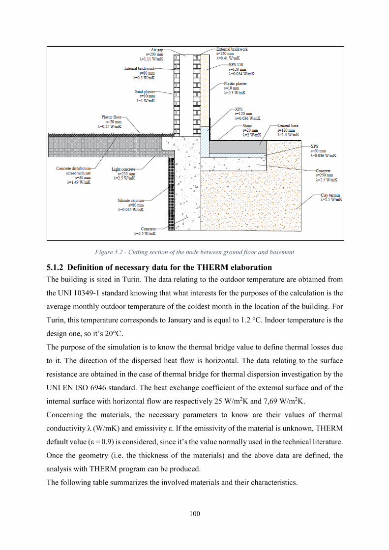
100
Figure 5.2 - Cutting section of the node between ground floor and basement
5.1.2 Definition of necessary data for the THERM elaboration
The building is sited in Turin. The data relating to the outdoor temperature are obtained from
the UNI 10349-1 standard knowing that what interests for the purposes of the calculation is the
average monthly outdoor temperature of the coldest month in the location of the building. For
Turin, this temperature corresponds to January and is equal to 1.2 °C. Indoor temperature is the
design one, so it’s 20°C.
The purpose of the simulation is to know the thermal bridge value to define thermal losses due
to it. The direction of the dispersed heat flow is horizontal. The data relating to the surface
resistance are obtained in the case of thermal bridge for thermal dispersion investigation by the
UNI EN ISO 6946 standard. The heat exchange coefficient of the external surface and of the
internal surface with horizontal flow are respectively 25 W/m2K and 7,69 W/m2K.
Concerning the materials, the necessary parameters to know are their values of thermal
conductivity λ (W/mK) and emissivity ε. If the emissivity of the material is unknown, THERM
default value (ε = 0.9) is considered, since it’s the value normally used in the technical literature.
Once the geometry (i.e. the thickness of the materials) and the above data are defined, the
analysis with THERM program can be produced.
The following table summarizes the involved materials and their characteristics.

101
Tab 5.1 - Material properties
5.2 THERM implementation
The first step to make in THERM environment is to prepare the file, by setting appropriate
values for the fields “Maximum % Error Energy Norm” replacing the value 10 with 2 and
“Maximum Iterations” replacing the value 5 with 20.
“Maximum % Error Energy Norm”
determines the granted percentage of
error. THERM will process the
simulation several times until this value
is reached. In general, a lower number
than the default value (10) increases the
accuracy of the calculation. “Maximum
Iterations” specifies the maximum
number of times the program will
change the mesh and repeat the calculation. In this case a higher value increases the accuracy.
5.2.1 Drawing
After this operation, the next step is to draw the geometry of the construction detail section to
be analyze. In this case the drawing is created in AutoCAD and then imported into the software
as a DXF file where it’s converted to make it directly usable. The drawing is indeed imported
as underlay and then traced so that each polygon represents a layer or a portion of the
construction.
Figure 5.3 - Therm File Options screen

102
The following operation consist of drawing the borderline to which the boundary conditions
will be subsequently associated. This operation allows an initial check that the converted
geometric model is free of errors. If the DXF file has been drawn correctly, the border will be
drawn, otherwise a window will inform the nature of the problem encountered: there could be
points of the geometry closest to the tolerance value and so the software proposes a rectification
solution to be accepted and confirmed. At this point the edges are drawn and the model is ready.
5.2.2 Materials’ definition
Having obtained the geometric representation of the construction node under examination, it’s
possible to proceed and attribute the corresponding materials to the various polygons that
characterize the stratigraphy. To do this it’s necessary to create the materials, characterize them
with the values of the parameters in table 6.1, save them in the corresponding library and then
associate them to the polygons. A different colour is matched to each material. Figure 5.4 shows
the model of the construction node with defined materials.
Figure 5.4 - Representation of the construction node with material defined
5.2.3 Boundary conditions
To proceed with the calculation, it is necessary to assign the boundary conditions. This means
to indicate to the program the different conditions in terms of temperature and surface resistance

103
that are present on the edges of the section (external and internal side of the wall, non-
conditioned basement ceiling and wall). Selecting one of the edges of the model, it’s possible
to see that the created edges are adiabatic. This condition must be maintained only in
correspondence of the cutting planes. The other boundary conditions must be created according
to UNI 10349-1:2016, as follows:
▪ External wall
Temperature = 1.2 °C since it’s the average daily temperature in the coldest month
(December) in Turin
Surface heat exchange coefficient = 25 W/m2K
▪ Internal wall
Temperature = 20°C
Surface heat exchange coefficient = 7.69 W/m2K
▪ Basement ceiling
Temperature = 10.5 °C
Surface heat exchange coefficient = 8 W/m2K (since the flux is vertical towards a
conditioned space, while for the wall it’s horizontal towards the terrain)
▪ Basement wall
Temperature = 10.5 °C
Surface heat exchange coefficient = 10 W/m2K (since the flux is horizontal towards the
terrain).
By choosing the simplified method, boundary conditions are defined by using only the
parameters described above. Once the boundary conditions have been defined, it’s necessary to
indicate to the program which edges to calculate along, that is, the surfaces affected by the
calculation of thermal transmittance. To do this it is necessary to create labels (U-factor
surfaces). In this case, the U-factor surfaces are three:
▪ INSIDE for “internal wall” boundary condition;
▪ OUTSIDE for “internal wall” boundary condition;
▪ BASEMENT for “basement ceiling” and “basement wall” boundary conditions.
If looking attentively at Figure 5.4, it’s possible to notice that edges have different colours: each
color corresponds to a boundary condition (red for “internal wall”, blue for “external wall”,
light blue for “basement ceiling”, green for “basement wall”, black for “adiabatic”).

104
5.2.4 Calculations
After drawing the cross section, specifying its materials and defining boundary conditions, it’s
possible to calculate the cross section’s thermal performance.
THERM is a two-dimensional (2D) finite-element heat-transfer analysis tool. It uses a steady-
state conduction algorithm, CONRAD, which is a derivative of the public-domain computer
program TOPAZ2D. THERM contains an automatic mesh generator that uses the Finite
Quadtree algorithm. It checks solutions for convergence and automatically adapts the mesh as
required using an error-estimation algorithm. THERM’s calculation routines evaluate
conduction and radiation from first principles, while convective heat transfer is approximated
using film coefficients obtained from engineering references. [17]
THERM automatically generates a finite-element mesh at the beginning of its calculations. The
cross section is broken into many discrete elements that are used to perform the finite-element
calculation. In the “Results Display Options” sheet, it’s possible to select the Finite Element
Mesh to be shown. The mesh used in the simulation is represented in Figure 6.5.
This reveals the areas in the cross section where the program has divided the building
component being modeled into a very fine mesh, determined by the cross-section geometry and
modified based on the percent error energy norm criterion.
Figure 5.5 - Mesh representation

105
5.2.5 Results visualization
Besides the Finite Element Mesh,
THERM allows to visualize different
results that can be selected by the “Results
Display Options” sheet shown in figure
6.6. Box “Draw Results” must be checked
for the graphic results to be drawn.
The choices in the section “Show” can be
activated one at a time. The setting will
determine what graphic results are drawn
by the program when the OK button is
clicked, as long as the Draw Results
option is checked.
▪ Isotherms - When the heat-transfer analysis is complete, THERM displays the lines of
isotherms through the cross section. They are useful for seeing where there are extreme
temperature gradients (isotherms very close together) that may lead to thermal stress or
structural problems. Isotherms are also useful for identifying hot or cold areas in the cross
section, in order to predict thermal degradation or condensation. Figure 6.7 shows
isotherms in the analysed cross section.
If selecting the “Show Min/Max temperatures” command, it’s possible to see the minimum
and maximum values of temperature reached in the cross section and in which points
they’re registered. In figure 5.7, the red cross represents the point with the highest
temperature (19,37 °C), the blue cross the one with the lowest temperature (1.32 °C).
By choosing the option “Temperature at cursor” from the “View” item in the toolbar, it’s
possible to visualize the temperature in any point in the cross section, just moving the arrow
on it. This is really useful to identify the temperature of the part of the section where the
thermal bridge is supposed to be (in this case the angle between the external wall and the
basement’s ceiling) and verify the presence of mould or condensation. These calculations
are made in the following paragraphs.
Figure 5.6 - THERM’s Results Display Options sheet

106
Figure 5.7 - Isotherms visualization
▪ Flux Vectors - The flux vector results indicate the amount and direction of heat flow
through the cross section. There is one flux vector for each mesh element. The length of
the vector corresponds to the amount of heat going through the element, which is a function
of both the size of the element and the magnitude of the heat flux. These results can only
be used for quantitative comparison with a uniform mesh. The direction of the arrow
indicates the direction of heat flow. This representation of the data is most useful for
determining the direction of heat flux.
▪ Color Infrared - The color infrared results show temperature gradients in the cross section.
Each temperature is represented by a different color; the cooler colors (purples and blues)
are low temperatures, and warmer colors (yellows and reds) are higher temperatures. This
can be seen in Figure 6.8.
▪ Color Flux Magnitude - The color flux magnitude results represent the heat flux vectors,
with the magnitude of the flux represented by color; the cooler colors (purples and blues)
are low flux and warmer colors (yellows and reds) are higher flux. This display does not
indicate the direction of the flux. It’s shown in Figure 6.9.

107
Figure 5.8 - Temperature gradients (°C) in the cross section
Figure 5.9 - Heat flux magnitude (W/m2) representation in the cross section
Results are obtained with an estimated error of 1.75%.

108
5.3 Thermal bridge linear transmittance calculation
By clicking on the Show U-factors button, the U-Factor window appears. Figure 6.10 shows it.
Consistently with the attribution of the three labels “Inside”, “Outside” and “Basement”, the
corresponding values are shown:
- U-Factor (thermal transmittance distributed over the length) [W/m2K]
- ΔT [°C]
- Length along which the transmittance is calculated [mm] (in this case the drop-down boxes
are set to “projected Y” since the focus of the analysis is the heat flow dispersion through
the vertical external wall, so only the lengths along the Y-axis needs to be considered)
- Heat Flow magnitude [W].
Figure 5.10 - U-factor window
The transmittance value calculated by Therm can be used to reach the value of the lineal thermal
transmittance that represents the thermal bridge.
In principle, it is a matter of calculating the heat exchange coefficient of the dispersing elements
(considered section) hypothesizing them homogeneous and comparing it to the heat exchange
coefficient calculated by Therm which otherwise will include the effect of the thermal bridge.
The difference between the two represents the value of the thermal bridge.
First, the calculation of the heat exchange coefficient that includes the effect of the potential
thermal bridge L2D is made, using the values calculated by Therm and multiplying them by the
length of the outer and inner edges of the external wall respectively.
Inside_L2D = U-factor inside * length inside = 1.7724 W/m2K * 1.1467 m = 2.0324 W/mK (27)
Outside_L2D = U-factor outside * length outside = 0.5643 W/m2K * 1.2560 m = 0.7088 W/mK (28)
The thermal transmittance of the external wall is calculated according to UNI EN 6946 and it’s
provided by Edilclima. It’s U-factor wall = 0.222 W/m2K.

109
Knowing this value, it’s possible to proceed with the calculation of the heat exchange
coefficient for homogeneous surfaces without thermal bridge.
Hi = U wall * length inside = 0.222 W/m2K * 1.1467 m = 0.2546 W/mK (29)
He = U wall * length outside = 0.222 W/m2K * 1.2560 m = 0.2788 W/mK (30)
The thermal bridge linear transmittance is therefore calculated for both the internal and external
edges as difference between the heat exchange coefficient that includes the effect of the
potential thermal bridge L2D and the one for homogeneous surfaces without thermal bridge.
Ψi = Inside_L2D - Hi = 2.0324 – 0,2546 = 1.7778 W/mK (31)
Ψe = Outside_L2D - He = 0.7088 – 0,2788 = 0.43 W/mK (32)
The value of the external thermal bridge (the one that usually need to be considered) is therefore
0.43 W/mK.
5.4 Condensation and mould formation test
In order to check if there’s risk of condensation or mould formation on the internal surface of
the wall, it’s important to check if 𝜃𝑠𝑖 > 𝑇𝑑𝑒𝑤 for condensation and if 𝑓𝑅𝑠𝑖 > 𝑓𝑅𝑠𝑖,𝑚𝑖𝑛 for mould
formation, where these terms have the meaning illustrated at the beginning of the chapter. In
both cases, 𝜃𝑠𝑖 needs to be known and can be calculated by Therm through the simulation. In
this case the temperature to consider is the one in correspondence to the thermal bridge,
meaning the one that is present at the edge between the external wall and the basement’s ceiling.
The temperature in this point can be read by selecting the “Temperature at cursor” and pointing
the cursor in this point. In this way, 𝜃𝑠𝑖 is determined and turns out to be 16.4 °C.
5.4.1 Condensation test
In order to exclude the possibility that superficial condensation will occur, the temperature of
the internal surface of the wall must be higher than the dew temperature at which the water
vapour present in the saturated indoor air condenses at constant pressure. which is to say 𝜃𝑠𝑖 >
𝑇𝑑𝑒𝑤. The dew temperature can be extracted from the psychrometric diagram by identifying the
point representative of indoor air (𝜃𝑖=20°C; RH = 50%) and then reading for RH = 100% on
the T axis the corresponding dew temperature Tdew. This operation in shown in figure 6.11. The
dew temperature for the above-mentioned indoor air state is 9.3 °C, so the condition 𝜃𝑠𝑖 > 𝑇𝑑𝑒𝑤
is verified. It’s possible to affirm that there’s no risk of superficial condensation.

110
Figure 5.11 - Dew temperature determination on psychrometric diagram
5.4.2 Mould formation test
In this case, given that the location is Turin, the minimum acceptable temperature that the
internal surface must have in order not to have mould formation, 𝜃𝑠𝑖,𝑚𝑖𝑛 is obtained by
Edilclima according to UNI EN ISO 13788 and is equal to 14.1 °C. The minimum value that
the temperature factor must have is the one corresponding to the month of January and it’s
defined as:
𝑓𝑅𝑠𝑖,𝑚𝑖𝑛 =𝜃𝑠𝑖,𝑚𝑖𝑛 − 𝜃𝑒
𝜃𝑖 − 𝜃𝑒=
14.1 − 1.2
20 − 1.2= 0.686
Since the internal surface temperature is 𝜃𝑠𝑖 = 16.4 °𝐶, the real temperature factor results
𝑓𝑅𝑠𝑖 =𝜃𝑠𝑖 − 𝜃𝑒
𝜃𝑖 − 𝜃𝑒=
16.4 − 1.2
20 − 1.2= 0.809
From these calculations, it turns out that 𝑓𝑅𝑠𝑖 > 𝑓𝑅𝑠𝑖,𝑚𝑖𝑛, so the necessary condition to exclude
the risk of mould formation is satisfied.
111
6. Results and conclusion
Both softwares provide the computation of the space heating and cooling powers and of the
space heating and cooling energy needs. Since they use different calculation methods, as
already mentioned, the results that they give are expected to be coherent (of the same order of
magnitude), since they refer to the same building in the same conditions, but different, because
they’re based on different equations. In order to get the higher level of coherence between
models, data have been constantly updated depending on the output given by the other, as
already illustrated for ventilation air flowrates and internal heat gains.
In this chapter, the iterative changes of input data inside the two models are described, then the
results given by both programs are shown and compared in terms of both power and energy,
graph of temperature and power trends are illustrated, a comparison between two climatization
strategies carried out in DesignBuilder is discussed and finally the compliance with Italian
normative is affirmed.
6.1 Data setting
As already specified, Edilclima and DesignBuilder follow different computational methods to
evaluate all the relevant information to perform an energy analysis, but these two programs also
have different interface and sections to input and set data. The two most relevant cases in which
this dissimilarity in entering data is evident are the ones mentioned in the previous sections:
definition of ventilation air flowrates and setting of internal heat gains. In both cases, at the
beginning, parameters in DesignBuilder have been defined on the basis of the data set on the
Edilclima model. Then, in a second time, since these differences in data setting led to
incoherence between the two models, the Edilclima file has been modified to meet the
DesignBuilder outputs. All the adaptations are made following logical reasonings and
calculations, even if they cause the non-compliance with the procedures indicated by the
normative for the definition of parameters.
6.1.1 Definition of ventilation supply and extraction flowrates
In this first case, initially the number of air flowrates for ventilation per space were defined in
Edilclima by choosing the option “Calculation according to UNI 10399”, which automatically
set a value in vol/h for each space, depending on its end use. In addition to this, Edilclima allows
to choose where to extract or to supply air, by selecting the desired option in the “Flowrates”
tab when defining the ventilation system. At first, extraction was made only from toilettes and
changing rooms on the basement, corridors and stairwell were spaces of air transit, while in all

112
the rest of the building air was only supplied. This was not compatible with DesignBuilder since
for all the group of zones, both supply and extraction are necessary otherwise the program
doesn’t work. In this way, in DesignBuilder the system turns out to be balanced, and that was
the opposite situation with respect to the configuration set in Edilclima. For this reason, the
system needed to be balanced. Moreover, the ventilation air flowrates for each space needed to
be changed, since the amount of dispersions for ventilation in Edilclima was excessively higher
than the one obtained from DesignBuilder. These two aspects led to the configuration shown in
Table 4.17, with a balanced system that has both supply and extraction in all the spaces. The
air flowrates in m3/h, there indicated, have been obtained by changing the calculation option of
ventilation load. The “Calculation with air changes” has been chosen and for all the spaces the
ventilation air flowrate for energy evaluations has been set to 0.5 vol/h, since this is the average
value computed by DesignBuilder. For estimations in terms of power, values have been left
equal to the ones indicated inside the normative (i.e. 8 vol/h for toilettes).
6.1.2 Definition of indicators for the calculation of internal heat gains
Edilclima makes distinction between the internal loads to be set for the cooling power
estimation and the ones necessary for the energy needs calculation, while DesignBuilder has
only one input option for both analyses. This caused a certain difficulty in defining coherent
values for all the entering data. Initially, in Edilclima, these steps were followed:
- zone internal loads [W/m2], that are necessary for energy calculations, have been left
unchanged and equal to the ones provided by UNI TS 11300 depending on the DPR 412
category (6.66 W/m2, 6 W/m2 and 10 W/m2 respectively for categories E.1, E.8 and E.4);
- space crowding indexes [persons/m2], which are needed for the design cooling power
evaluation, have been defined so that in each space there is a realistic number of people;
- space electrical densities of power [W/m2], that are necessary for cooling power estimation,
were set to 0.
Once in DesignBuilder, a value for occupancy in [persons/m2], one for equipment and
computers and one for lighting [W/m2] were required. So:
- occupancy has been calculated as illustrated in section 4.5.2 and table 4.19;
- equipment and computers loads have been determined as reasonably true portion (0%-
20%-40% depending on the kind of space) of the zone internal loads defined in Edilclima;
- lighting needed to be defined for the evaluation of the design cooling power, so LEDs have
been chosen as lamps and in this way the power density for lighting has been automatically
set to 2.5 W/m2, which is the one assigned to the type of lighting unit.

113
According to these new data entered in the DesignBuilder model, the Edilclima one needed to
be changed so the space electrical power density was changed from 0 to the sum of power
densities for equipment and lighting defined in DesignBuilder.
A strong dissimilarity in total internal loads was still present between the two models, since this
modification didn’t affect the energy evaluation. Zone internal loads have yet been changed,
following this method:
- from the results in terms of energy, the different internal loads (people, lighting and
equipment) for each zone were extracted;
- they were summed up and divided by 1000 and by the number of hours which the
simulation refers to (8760 h, since it was a yearly calculation) in order to get the average
power given by these contributions;
- values of average power were finally divided for the net surface area of the zone, in order
to get the most coherent value of zone internal loads in [W/m2] with respect to the Edilclima
one.
Zone internal loads and the necessary data for their calculation are shown in table 6.1 and 6.2.
It’s possible to notice how the calculated indexes differ from the one initially input according
to normative indications.
These are the final data entered for internal loads: no other changes have been made since there
is no better way to calculate them.
Tab 6.1 - Edilclima zone internal loads calculation (a)

114
Tab 6.2 - Edilclima zone internal loads calculation (b)
6.2 Design space heating and cooling powers
In both softwares, the computation of the space heating and cooling powers overlooks the
presence of any HVAC system. For space heating, the calculation is based on the dispersions
occurring in the building by transmission and natural ventilation, and the design heating power
ids obtained as sum of the dispersed heat flows multiplied by a security factor, that in both
models has been assumed equal to 1.12. For space cooling, the computation is focused on latent
and sensible internal and solar heat gains evaluations in both models, even if the approaches
are not exactly the same. Both evaluations have been made basing on the same net and gross
volumes, since, as mentioned in chapter 4, by the tabular method, these values were entered
manually in Edilclima and are equal to the ones estimated by DesignBuilder.
The main differences stand in:
- the way in which they’re calculated: Edilclima uses a quasi-steady state method, giving
constant monthly values to parameters, while DesignBuilder performs a dynamic
calculation and so updates those values on a much smaller period of time.
Lab 1 55,22
Lab 2 47,25
Lab 3 18,00
Lab 4 18,00
Lab 5 18,00
Lab 6 48,97
Lab 7 22,02
Lab 8 12,24
Lab 9 17,89
Lab 10 17,85
Lab 11 17,93
Lab 12 22,63
Lab 13 21,17
Lab 14 21,59
Lab 15 26,39
Lab 16 19,76
Lab 17 19,51
Lab 18 23,04
Lab 19 18,76
Lab 20 67,21
Relax area 92,14
Open space 240,67
Copyprint 21,28
Laboratory 1 45,89
Laboratory 2 21,61
Laboratory 3 41,84
Laboratory 4 21,79
Laboratory 5 21,93
Laboratory 6 21,93
Laboratory 7 21,93
Laboratory 8 70,04
Informal meeting 1 7,44
Informal meeting 2 7,49
Informal meeting 3 7,45
Open space 151,15
Copyprint 1 6,55
Equipment
heat gains
[kWh]
Zone internal
loads [kWh]Space
Zone internal
loads [W/m2]
Space net
surface area
[m2]
Zone net
surface area
[m2]
People heat
gains [kWh]
Lighting
heat gains
[kWh]
First floor
Edilclima ZoneDesignBuilder
Zone
887,52 11932,17
447,04 7810,93 3500,29 3360,28 14671,49Second floor Second floor 3,75
First floor 3,29 25552,746949,27 6671,30

115
- outdoor project temperatures; since Edilclima assumes the value indicated by normative,
while DesignBuilder considers another value included inside the weather file;
- definition of internal gains: Edilclima distinguishes values of internal gains (in terms of
W/m2 or pers/m2) for space cooling power calculation and energy needs calculations; in
DesignBuilder this distinction is absent, so, even if internal gains are determined following
a logical path to be coherent with Edilclima’s definitions, there’s a sort of uncertainty on
the equivalence of them. In addition to this, for the calculus of space cooling power,
DesignBuilder explicitly defines a security factor that multiplies by the sum of latent and
sensible heat gains; Edilclima apparently doesn’t consider a security factor in this case.
- solar gains are elaborated in different ways by the two programs and it’s not possible to
operate on them, so intrinsic differences are necessarily present.
All this obviously leads to differences in the results.
In the following figures and tables, the results obtained respectively from Edilclima and
DesignBuilder computations are shown.
Figure 6.1 - Edilclima results in terms of heating power

116
Tab 6.3 - DesignBuilder results in terms of heating power
As it can be seen in Figure 6.1, the design space heating power computed by Edliclima is 97.8
kW, while the one calculated by DesignBuilder (Table 6.3) is equal to 109.13 kW. This means
that the dynamic method computes a design heating power that is higher than the one obtained
with the quasi-steady method, which is used for the sizing of the plant.
This difference can be attributed to the dissimilar way in which building components are
defined, meaning by the fact that boundary conditions in Edilclima are manually entered, while
in DesignBuilder they’re automatically implemented. This could be the cause of a difference in
transmission dispersions and so in the evaluation of the total design space heating power.
Tab 6.4 - Edilclima results in terms of cooling power
Zone Space
Comfort
temperature
(°C)
Heat loss in
steady regime
(kW)
Heat loss in
Intermittent
Mode (kW)
Design
heating power
(kW)
Design heating
power per floor
area (W/m2)
Alloggio Custode Alloggio Custode 19,28 1,48 0,00 1,65 43,89
Scale ingresso Scale ingresso 18,76 0,32 0,00 0,36 43,12
Bagno 1P 1 19,07 1,25 0,00 1,40 64,12
Bagno PT 1 19,46 1,17 0,00 1,31 57,86
Bagno PT 2 19,68 1,31 0,00 1,46 53,77
Bagno 1P 2 19,60 1,15 0,00 1,28 55,05
Bagni 2P 19,26 1,48 0,00 1,66 56,67
Ripostiglio 1 19,42 0,04 0,00 0,04 11,75
Ripostiglio 2 19,38 0,05 0,00 0,06 16,29
Piano Terra 19,30 24,44 0,00 27,37 35,97
Magazzino PT 15,20 2,66 0,00 2,98 11,84
Primo Piano Primo Piano 19,29 28,17 0,00 31,55 35,55
Zona Bar Zona Bar 18,93 7,56 0,00 8,47 56,55
Secondo Piano Secondo Piano 18,80 19,35 0,00 21,67 48,47
Sale riunioni PT Sale riunioni PT 18,75 4,53 0,00 5,07 64,37
Piano interrato Spogliatoi Pint 19,82 2,50 0,00 2,80 33,01
109,13BUILDING DESIGN HEATING POWER
Servizi igienici
Piano Terra
Zone SpaceTime of
the day
Load due to
irradiation
Qirr [W]
Load due to
transmission
Qtr [W]
Load due to
ventilation
Qv [W]
Internal
loads
Qc [W]
Global
sensible load
Qgl,sen [W]
Global
latent load
Qgl,lat [W]
Global load
Qgl [W]
Alloggio Custode AlloggioCustode 16 188 464 536 718 1269 637 1906
Scale ingresso ScaleIngresso 16 97 103 209 0 275 133 408
Bagno PT 1 16 0 21 313 429 406 356 762
Bagno PT 2 16 166 240 260 356 726 296 1022
Bagno 1 P1 16 166 101 250 344 576 285 861
Bagno 1P 2 16 3 144 309 367 493 332 825
Bagni 2P 16 2 175 280 374 516 316 832
Ripostigli 16 0 79 96 0 113 61 174
Piano Terra 16 39345 3279 13925 10899 54299 13152 67451
Magazzino PT 16 4635 363 1646 1311 6594 1361 7955
Primo Piano Primo Piano 16 6159 3340 21160 12456 25034 18081 43115
Zona Bar ZonaBar 16 564 952 6383 3802 6180 5520 11700
Secondo Piano Secondo Piano 16 8475 1885 9965 7433 18425 9331 27756
Sale riunioni PT Sale Riunioni PT 16 110 168 1090 1478 1766 1080 2846
Piano interrato Spogliatoi Pint 16 0 760 1197 1321 1956 1320 3276
TOTAL 16 59910 12074 57619 41288 118628 52261 170889
Servizi igienici
Piano Terra

117
Tab 6.5 - DesignBuilder results in terms of cooling power
In this case the dynamic calculation made by DesignBuilder gives a value (121.68 kW) for the
design cooling power that is lower than the one provided by Ediclima (170,89 kW).
In particular, it’s possible to notice how in Edilclima results, the design space cooling power is
almost the double of the design space heating power (and that’s a usual situation that
professionals get when they design recurring to the approach described in the normative), while
instead DesignBuilder gives similar values for these powers (they differ only for 12.55 kW).
This difference in the entity of the design cooling powers computed by the two softwares can
be linked to contemporaneity factors. In DesignBuilder, in fact, schedule for occupancy and
equipment utilization have been defined so that internal loads are not constant during the day.
This means that, even if the hour of the summer day in which the peak of cooling load is reached
is the same in both cases (4 p.m.), this peak is lower in the dynamic calculation due to the
contemporaneity factor, that in Edilclima is not considered (even if there is the possibility to
define a value for this index). In addition to this, as previously mentioned, climatic data are not
the same in the two softwares and this can affect the solar loads, so that they come up to be
different. Finally, DesignBuilder determines on its own which is the most critical period for the
building in terms of solar and internal loads and it chooses the most critical day inside the
interval of time indicated before the computation (that in this case goes from July,15 to
September 15). This day occurs in the month of August. In Edilclima, the design space cooling
power is computed in the peak month, which for the selected location (Turin) is July. This could
be an additional cause for this disparity.
Zone SpacePeak cooling
time
Indoor air
temperature
(°C)
Maximum
daily
operative
temperature
(°C)
Humidity
(%)
Sensible
load
(kW)
Latent
load
(kW)
Total
cooling load
(kW)
Design
cooling
power
(kW)
Design
cooling load
per floor area
(W/m2)
Alloggio Custode Alloggio Custode Aug 16:00 26 26,7 59,8 0,93 0,67 1,61 1,8 47,7
Scale ingresso Scale Ingresso Aug 16:00 26 27,3 41,7 0,7 0 0,7 0,78 94,6
Bagno PT 1 Aug 16:00 26 26,7 61,2 0,72 0,44 1,16 1,3 57,4
Bagno PT 2 Aug 16:00 26 25,8 77,0 0,45 0 0,45 0,5 18,3
Bagno 1P 1 Aug 16:00 26 27,0 51,8 0,84 0,6 1,44 1,61 73,9
Bagno 1P 2 Aug 16:00 26 26,5 75,7 0,53 0,03 0,56 0,62 26,7
Bagni 2P Aug 16:00 26 26,6 66,4 0,71 0,28 0,99 1,11 37,8
Ripostiglio 1 Aug 16:00 26 26,4 41,7 0,02 0 0,02 0,02 6,2
Ripostiglio 2 Aug 16:00 26 26,3 41,7 0,02 0 0,02 0,02 6,2
Piano Terra Aug 16:00 26 26,8 51,9 16,17 11,37 27,54 30,85 40,5
Magazzino PT Aug 16:00 28 28,6 38,0 3,9 0,54 4,44 4,97 19,8
Primo Piano Primo Piano Aug 16:00 26 26,9 46,5 24,56 13,68 38,24 42,83 48,3
Zona Bar Zona Bar Aug 16:00 26 26,9 56,2 3,91 2,32 6,23 6,98 46,6
Secondo Piano Secondo Piano Aug 16:00 26 27,1 47,3 12,91 8,12 21,02 23,54 52,7
Sale riunioni PT Sale Riunioni PT Aug 16:00 26 26,8 48,7 2,47 1,76 4,24 4,75 60,2
Piano interrato Spogliatoi Pint Aug 16:00 24,6 24,4 85,3 0 0 0 0 0,0
TOTAL Aug 16:00 25,6 28,6 54,4 68,84 39,81 108,66 121,68 36,8
Servizi igienici
Piano Terra

118
6.3 DesignBuilder outputs
DesignBuilder allows the user to choose which of the available output he wants to compute and
display at the end of the dynamic simulation, in graphical or tabular form (depending on the
physical quantity in analysis). Here the some of these results are illustrated.
Figure 6.2 - Temperatures in the building on a typical winter week
Figure 6.2 shows the mean indoor air temperature and radiant temperature of the building, and
their mean value which is the operative temperature in a typical winter day. The indoor air
temperature reaches a value lower than the designed 20°C because all the spaces of the building
are considered, even the unconditioned ones, which are at a very low temperature since it’s
winter time, so the effect is a decrease of the global air temperature. From figure 6.2 it’s possible
to notice how the HVAC system is scheduled to start at 7.00 a.m. (at that time temperature starts
to rise), increases at steps, since it has been defined so, and reaches its maximum at 2.30 p.m.,
because of solar and internal gains. At 7.00 p.m. the HVAC system turns off, the temperature
suddenly drops and after an hour continues decreasing slowly till it reaches almost 16 °C. This
temperature corresponds to the mean attenuation value of temperature of the building: for all
the spaces (except for the storage room) the attenuation temperature during nights and
weekends is set to 18°C, but because of the unconditioned spaces, on average it results to be
16°C. This is what happens in weekdays. During the weekends (as it’s possible to see on Sunday
20/01 and on Saturday 26/01), the HVAC system is kept on attenuation mode, so the oscillations
of temperatures values are limited to an interval of less than 1 °C; this is determined by
oscillation of temperatures of the unconditioned spaces, which are sensible to the outdoor
temperature variation.

119
Figure 6.3 - Solar and Internal heat gains on a typical winter week
Figure 6.3 shows the trend of the space heating power through the days on a typical winter
week. On weekdays, from the 21st to the 25th of January, internal loads are constant. The most
important contribution (with peaks of 22 kW) is given by people that occupies the building and
assumes this particular trend because of the schedule that was assigned to it, that provides a
lower number of persons inside the building in the lunch time. The small amount of occupation
load on Saturday (represented by January 26th) is assigned in order to take into account possible
presence of workers out of working hours. Lighting is on only during the working hours, so its
contribution is constant (7 kW), and together with computers and other electrical equipment
give a significant heat load. That obviously affects the trend of space heating power, which is
lower when the building is occupied, because internal and solar gains contribute to increase the
indoor air temperature, and is higher during the night-time and on weekends, since it has to
keep the attenuation temperature that has been set (18°C) without the help of gains. Solar heat
gains have this outline because on working days they are controlled by shut systems, while on
weekdays they are free to come in.
Similar considerations can be made for a typical summer week (figure 6.4), which in this case
is represented by days from August 17th to 23rd, since no holiday is provided for this building.
On summer time, space cooling power compensates for internal and solar heat loads, which are
scheduled as previously described for the winter case. Again, it’s possible to see how all the
internal loads (except for a small contribution given by occupation) are absent during weekends

120
(August 17th and 18th), while solar loads are left uncontrolled and so the space cooling system
needs to supply cooling power to keep the indoor environment at the attenuation temperature
of 28°C.
Figure 6.4 - Solar and Internal heat loads on a typical summer week
DesignBuilder allows also to see heat gains and losses through building components, but these
results are most significant in terms of energy rather than power, so they are displayed in the
next section.
6.4 Energy evaluations and comparison between models
In this section, the results in terms of energy obtained from both programs are illustrated. In
particular, results from Edilclima are shown in tabular form, while the ones from DesignBuilder
are graphically presented through bars diagrams. The comparison between the two models is
focused on the amount of energy dispersed by transmission and ventilation in the space heating
season (going from October 15 to April 15), on the values of internal and solar gains again in
winter time, and finally on the total energy consumption, both in terms of net and source energy.
6.4.1 Dispersions by transmission and ventilation
Both Edilclima and DesignBuilder calculates energy losses by transmission on the basis of
thermal transmittances, surface areas and orientation of the building components together with
climatic data, so once the building envelope is defined in the most similar way in the two
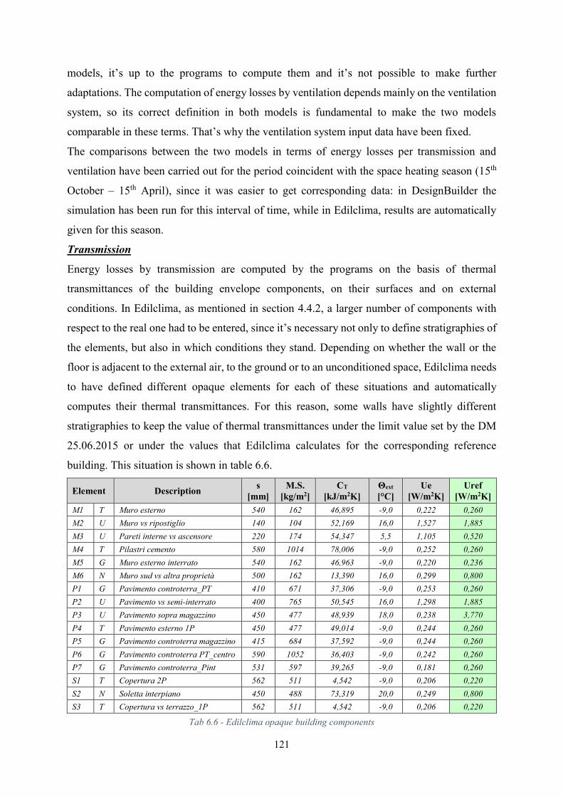
121
models, it’s up to the programs to compute them and it’s not possible to make further
adaptations. The computation of energy losses by ventilation depends mainly on the ventilation
system, so its correct definition in both models is fundamental to make the two models
comparable in these terms. That’s why the ventilation system input data have been fixed.
The comparisons between the two models in terms of energy losses per transmission and
ventilation have been carried out for the period coincident with the space heating season (15th
October – 15th April), since it was easier to get corresponding data: in DesignBuilder the
simulation has been run for this interval of time, while in Edilclima, results are automatically
given for this season.
Transmission
Energy losses by transmission are computed by the programs on the basis of thermal
transmittances of the building envelope components, on their surfaces and on external
conditions. In Edilclima, as mentioned in section 4.4.2, a larger number of components with
respect to the real one had to be entered, since it’s necessary not only to define stratigraphies of
the elements, but also in which conditions they stand. Depending on whether the wall or the
floor is adjacent to the external air, to the ground or to an unconditioned space, Edilclima needs
to have defined different opaque elements for each of these situations and automatically
computes their thermal transmittances. For this reason, some walls have slightly different
stratigraphies to keep the value of thermal transmittances under the limit value set by the DM
25.06.2015 or under the values that Edilclima calculates for the corresponding reference
building. This situation is shown in table 6.6.
Element Description s
[mm]
M.S.
[kg/m2]
CT
[kJ/m2K]
Θext
[°C]
Ue
[W/m2K]
Uref
[W/m2K]
M1 T Muro esterno 540 162 46,895 -9,0 0,222 0,260
M2 U Muro vs ripostiglio 140 104 52,169 16,0 1,527 1,885
M3 U Pareti interne vs ascensore 220 174 54,347 5,5 1,105 0,520
M4 T Pilastri cemento 580 1014 78,006 -9,0 0,252 0,260
M5 G Muro esterno interrato 540 162 46,963 -9,0 0,220 0,236
M6 N Muro sud vs altra proprietà 500 162 13,390 16,0 0,299 0,800
P1 G Pavimento controterra_PT 410 671 37,306 -9,0 0,253 0,260
P2 U Pavimento vs semi-interrato 400 765 50,545 16,0 1,298 1,885
P3 U Pavimento sopra magazzino 450 477 48,939 18,0 0,238 3,770
P4 T Pavimento esterno 1P 450 477 49,014 -9,0 0,244 0,260
P5 G Pavimento controterra magazzino 415 684 37,592 -9,0 0,244 0,260
P6 G Pavimento controterra PT_centro 590 1052 36,403 -9,0 0,242 0,260
P7 G Pavimento controterra_Pint 531 597 39,265 -9,0 0,181 0,260
S1 T Copertura 2P 562 511 4,542 -9,0 0,206 0,220
S2 N Soletta interpiano 450 488 73,319 20,0 0,249 0,800
S3 T Copertura vs terrazzo_1P 562 511 4,542 -9,0 0,206 0,220
Tab 6.6 - Edilclima opaque building components

122
The letters in the first column indicates the type of element: M stands for walls, P for floors, C
for ceilings/roof. The ones in the second column refer to the boundary conditions: T means that
the structure disperses to the outside environment, G towards the ground, U towards non-
conditioned rooms or solar greenhouses and N towards adjacent areas or apartments. The last
column shows the corresponding U-value in the reference building that needs to be respected.
In DesignBuilder, this distinction is not available since only one stratigraphy can be entered for
the elements that the program automatically recognizes (Ground floor, Roof, External wall,
Internal partition, Inter-storey slab) whose thermal transmittances are the ones indicated in
section 4.5.2 and stratigraphies are the ones shown in section 4.3.
The following table shows the values of thermal energy losses computed by Edilclima and
DeisgnBuilder divided per type of components.
Tab 6.7 - Energy losses by transmission
The two programs give quite different results: the energy losses by transmission computed by
Edilclima are almost the double of the one calculated by DesignBuilder. In both cases the
biggest contribution is given by glazed components and the dispersed energy is almost equally
divided between glazed and opaque components. This big difference can be attributed to the
above-mentioned differences, since in DesignBuilder simplification of the types of the
stratigraphy was adopted and it makes more sophisticated calculations for the determination of
thermal transmittances. In addition to this, the use of different climatic data also plays its part.
Figure 6.5 - Bar chart for energy transmission losses comparison
kWh % kWh %
External walls 18678,81 19,0 10492,08 22,2
Floors 20149,95 20,4 611,47 1,3
Roof/ceilings 15277,93 15,5 10178,04 21,5
Windows 44450,32 45,1 26048,21 55,0
TOTAL 98557,00 100 47329,8 100
Energy losses by transmission
Edilclima DesignBuilderBuilding component

123
Ventilation
Energy losses by ventilation are automatically calculated by both softwares and, as already
mentioned, they strictly depend on the type of ventilation system that is considered and on
which air flowrates it works with. Here in DesignBuilder, a VAV system has been input, while
on Edilclima it’s not explicitly stated, but should be of the same kind. Air flowrates have been
set as previously described, so the systems are comparable.
Figure 6.6 shows the trend of energy losses by ventilation as computed by both programs.
Figure 6.6 - Energy losses by ventilation
Total dispersions by ventilation results to be equal to 50928 kWh and 45717 kWh according
respectively to Edilclima and DeisgnBuilder. In both cases, the higher value of energy
dispersions per ventilation is on January, which is the most critical month of the winter season.
The trends are very similar for the extreme month of the interval, while differs in the central
part of the season. This again can be partly input to the different climatic data used in the two
programs (in Edilclima, external conditions are more critical than the ones adopted in
DesignBuilder), to the non-identical values of air flowrates and to the different computational
methods. Probably also the heat recovery module of the AHU, handled differently by the two
software, influences the outputs.
6.4.2 Solar and internal heat gains
Even the comparisons between the two models in terms of internal and solar heat gains have
been carried out for the space heating season, for the same reason.
Solar heat gains
Both programs automatically compute solar heat gains once location, orientation, glazed
surfaces and shutting system have been defined. They use completely different approaches for

124
the definition of solar heat gains, so it’s not possible to operate on them in any way. Edilclima’s
approach overestimates solar heat gains, so a comparison for this object is not consistent. For
the records, the values of solar heat gains calculated by the two programs are the following:
61374 kWh in Edilclima against 11930 kWh in DesignBuilder.
Internal heat gains
Internal heat gains strongly depend on the input data entered by the user. It’s the most
complicated part to be set coherently in the two softwares. By entering data in Edilclima and
DesignBuilder as described in section 6.1.2, comparable results have been obtained. The
internal heat gains that are considered occupation, lighting and equipment. In DesignBuilder a
small contribution is given by the food preparation inside the janitor’s house and the coffee
break area, but it’s not considered here since it was not used for the definition of internal heat
gains in the Ediclima model. Fig 6.7 and table 6.8 shows the monthly amount of internal heat
gains computed by the two programs and highlight in which months they are higher or lower.
Tab 6.8 - Internal heat gains defined per month
Figure 6.7 - Internal heat gains trend during the heating season
kWh % kWh %
October 3680 9,3 3946 9,3
November 6494 16,4 6790 16,0
December 6711 16,9 7345 17,3
January 6711 16,9 7780 18,3
February 6061 15,3 6674 15,7
March 6711 16,9 6629 15,6
April 3247 8,2 3314 7,8
TOTAL 39615 100 42476 100
Month
Internal heat gains
Edilclima DesignBuilder

125
In this case, the difference between the two models turns out to be small (less than 3000 kWh)
which is a good result if considering the different approaches adopted. In both cases, the higher
contribution in terms of internal heat gains is reached in January, while the lower is registered
in April (even because only 15 days of this month are included in the heating season). The
trends are similar; the only curious thing can be pointed out in March. Here, DesignBuilder
registers a small decrease in internal heat gains with respect to February, while Edilclima
evaluates an amount of internal gains that is equal to the maximum value reached in December
and January.
In figure 6.8, the amount of internal gains coming from the different “sources” is shown divided
per month. The highest contribution is given by occupation.
Figure 6.8 - Internal heat gains contributions
6.4.3 Site and source energy
Evaluation on source energy have been made on a yearly basis, comparing total energy needs.
The consumption in terms of source energy can be easily found in the dedicated sheet on the
“Source energy results” tab on Edilclima. Here, the total source energy consumption is divided
in renewable and non-renewable contributions, in order to check the compliance with DLgs
n.28/2011. Results are resumed in figure 6.9 as Edilclima produce them.
Figure 6.9 - Source energy consumption according to Edilclima
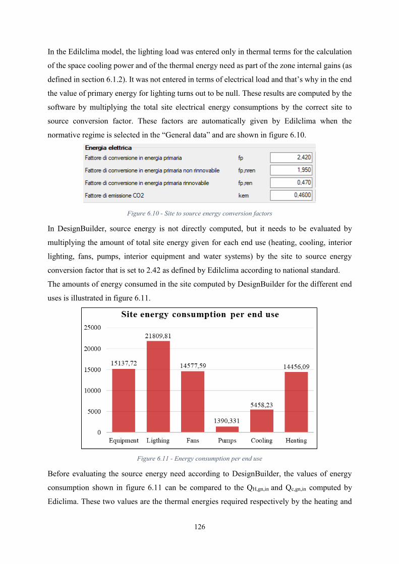
126
In the Edilclima model, the lighting load was entered only in thermal terms for the calculation
of the space cooling power and of the thermal energy need as part of the zone internal gains (as
defined in section 6.1.2). It was not entered in terms of electrical load and that’s why in the end
the value of primary energy for lighting turns out to be null. These results are computed by the
software by multiplying the total site electrical energy consumptions by the correct site to
source conversion factor. These factors are automatically given by Edilclima when the
normative regime is selected in the “General data” and are shown in figure 6.10.
Figure 6.10 - Site to source energy conversion factors
In DesignBuilder, source energy is not directly computed, but it needs to be evaluated by
multiplying the amount of total site energy given for each end use (heating, cooling, interior
lighting, fans, pumps, interior equipment and water systems) by the site to source energy
conversion factor that is set to 2.42 as defined by Edilclima according to national standard.
The amounts of energy consumed in the site computed by DesignBuilder for the different end
uses is illustrated in figure 6.11.
Figure 6.11 - Energy consumption per end use
Before evaluating the source energy need according to DesignBuilder, the values of energy
consumption shown in figure 6.11 can be compared to the QH,gn,in and Qc,gn,in computed by
Ediclima. These two values are the thermal energies required respectively by the heating and

127
the cooling generation systems. Since Edilclima doesn’t distinguish the energy consumption
due to fans and pumps like DesignBuilder does, the values given by DesignBuilder for these
uses are distributed by adding 7920 kWh to the energy consumption for heating, since it’s the
amount of energy requested by fans and pumps in the heating season, and the rest to the energy
need for cooling. Table 6.9 shows the site energy consumptions evaluated by DesignBuilder
for each use and compares them with the energy need of the generations systems inside the
Edilclima model. The thing to say is that data from DesignBuilder are in terms of electrical
energy that the system needs to heat/cool air and water, while Edilclima ones are kWh of energy
needed by the heating and cooling systems and auxiliaries.
Tab 6.9 - Energy needs for heating and cooling
Now it’s possible to evaluate the source energy needs for heating and cooling according to
DesignBuilder by multiplying the values in table 6.9 by 2.42 and to compare them with the ones
computed by Edilclima, shown in figure 6.9. Results are reported in table 6.10.
Tab 6.10 - Source energy needs
Globally, the DesignBuilder model provides a lower amount of source energy needs with
respect to the Edilclima one for heating, cooling and ventilation systems.
One last observation is left to the PV generation. Coherently with the overestimation of solar
heat gains, even solar PV production is higher in Edilclima (52609 kWh) than in DesignBuilder
(45438 kWh).
6.5 Comparison between different air conditioning strategies
As additional observations, two more analysis have been carried out. The first one regards the
type of ventilation system, with the focus on the energy consumption that each of them
implicates. The second analysis is dedicated to the evaluation of a possible integration of more
terminal units, centred on the ground floor which is the most significant zone of the building.

128
6.5.1 VAV and CAV in comparison
CAV and VAV are the acronyms respectively for constant air volume and variable air volume
(VAV) systems. CAV systems supply a constant airflow at variable temperature, while VAV
systems supply a variable airflow at constant temperature.
In general, CAV systems are less expensive and simpler to design and install, while VAV
systems offer superior performance and energy savings for a higher upfront cost. Usually, VAV
ventilation is the best option because long-term energy savings outweigh the additional system
cost, but in the cases of applications where the ventilation load shows little variation, CAV is
recommended. In this case, the economic side has not been considered, the focus is on the
comparison of the performances of the two kind of systems. In both cases, single duct systems
have been simulated. The following diagram shows the differences in terms of energy
consumption that exist between the two types of system.
Figure 6.12 - VAV and CAV energy consumptions in parallel
As predictable, VAV consumes a lower amount of energy. The items that can be allocated to
the conditioning and ventilation systems are fans, pumps, cooling and heating, which in fact are
the only indicators that varies between the two. Electrical equipment and lighting energy needs
are a constant of the situation, since they are characteristics of the building and of the schedule
set for them, while generation from the PV system depends only on that system and on climatic
data, which of course are the same. The total energy consumption for the two systems, intended
as sum of energy need for fans, pumps, cooling and heating are 35882 kWh for VAV system
and 97059 kWh for CAV system, so it’s evident how the VAV solution reduces the energy

129
consumption with respect to a more conventional CAV system. In particular, the biggest
difference lays in the heating and fans consumptions, due to the fact that CAV system deals
with a larger amount of air and so the energy need to treat it is higher.
6.5.2 Addition of radiant heated floor in the ground floor
After having assessed that VAV system is more efficient than the CAV one, another analysis
has been performed focusing on the type of HVAC terminal units. In particular, the object of
the analysis is the ground floor, characterized by a large open space with high ceiling, which is
at first conditioned only through the air system as all the other spaces and then conditioned in
winter time through the addition of radiating panels on the floor. So, the idea is the one to
evaluate the effects in terms of thermal comfort of the radiant heat floor.
The parameters that are considered are the Fanger index, the relative humidity and the indoor
air temperature in both cases.
Figure 6.13 illustrates the results obtained for the two situations in a typical winter week (from
January 20 to January 26).
Figure 6.13 - Comparison between comfort parameters with and without radiant heating
As it’s possible to see, the adding of radiant heating improves comfort parameters: indoor air
temperature is closer to the set point value, relative humidity reaches the same maximum value
but is lower when the building is unoccupied and the Fanger index gets better, even if it’s not
exceptional. This means that a combined solution with air conditioning and radiant heating
could give best results in terms of comfort, even if consumptions would be probably worse.
6.6 Law verifications
After completing the data input procedure and performing the calculations for the building's
useful and primary energy, by going to the “Legislative Verifications” section, it’s possible to
compare the building's performance with the minimum requirements imposed by national
legislation. That’s allowed by the module EC701 which can carry out the legal checks and the

130
technical report according to the Interministerial Decree 26.6.2015 and the Legislative Decree
03.03.2011, n. 28.
Legislative Decree n. 28 of 03.03.2011 Verifications
In order to visualize the verifications to be respected according to the DLgs n. 28/2011 it is
necessary to identify the "Type of intervention" which in this case is “Complete renovation of
building elements for buildings with a surface area > 1000 m2”. Annex 3 of DLgs n.28/2011
prescribes the verification of total coverage (heating, cooling and DHW services) from
renewable sources and of coverage of DHW from renewable sources (50% of the expected
consumption of DHW must be covered by renewable sources). They are calculated in
accordance with UNI/TS 11300-5 and obtained as the ratio between renewable primary energy
and total primary energy. Annex 3 of DLgs n. 28/2011 also prescribes the obligation to install
systems to produce electricity from renewable sources, serving the electrical uses of the
building, in the case of new buildings or buildings undergoing major renovation.
For this verification to be positive, the value of the electrical power installed in the building
must be higher than the value obtained as S/K where K is a coefficient that varies according to
the date of application for the building permit and S is the floor area of the building at ground
level, expressed in m2.
Figure 6.14 shows that all these parameters are verified as prescribed by DLgs n. 28/2011.
Figure 6.14 - DLgs n.28/2011 verifications
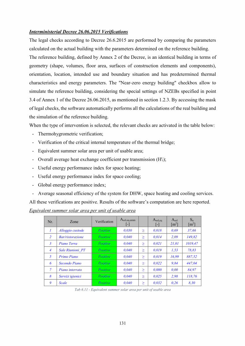
131
Interministerial Decree 26.06.2015 Verifications
The legal checks according to Decree 26.6.2015 are performed by comparing the parameters
calculated on the actual building with the parameters determined on the reference building.
The reference building, defined by Annex 2 of the Decree, is an identical building in terms of
geometry (shape, volumes, floor area, surfaces of construction elements and components),
orientation, location, intended use and boundary situation and has predetermined thermal
characteristics and energy parameters. The "Near-zero energy building" checkbox allow to
simulate the reference building, considering the special settings of NZEBs specified in point
3.4 of Annex 1 of the Decree 26.06.2015, as mentioned in section 1.2.3. By accessing the mask
of legal checks, the software automatically performs all the calculations of the real building and
the simulation of the reference building.
When the type of intervention is selected, the relevant checks are activated in the table below:
- Thermohygrometric verification;
- Verification of the critical internal temperature of the thermal bridge;
- Equivalent summer solar area per unit of usable area;
- Overall average heat exchange coefficient per transmission (H't);
- Useful energy performance index for space heating;
- Useful energy performance index for space cooling;
- Global energy performance index;
- Average seasonal efficiency of the system for DHW, space heating and cooling services.
All these verifications are positive. Results of the software’s computation are here reported.
Equivalent summer solar area per unit of usable area
Nr. Zone Verification Asol,eq,amm
[-]
Asol,eq
[-]
Asol
[m2]
Su
[m2]
1 Alloggio custode Positive 0,030 ≥ 0,018 0,69 37,66
2 Bar/ristorazione Positive 0,040 ≥ 0,014 2,09 149,82
3 Piano Terra Positive 0,040 ≥ 0,021 21,01 1019,47
4 Sale Riunioni_PT Positive 0,040 ≥ 0,019 1,53 78,83
5 Primo Piano Positive 0,040 ≥ 0,019 16,99 887,52
6 Secondo Piano Positive 0,040 ≥ 0,022 9,84 447,04
7 Piano interrato Positive 0,040 ≥ 0,000 0,00 84,97
8 Servizi igienici Positive 0,040 ≥ 0,025 2,98 118,76
9 Scale Positive 0,040 ≥ 0,032 0,26 8,30
Tab 6.11 - Equivalent summer solar area per unit of usable area
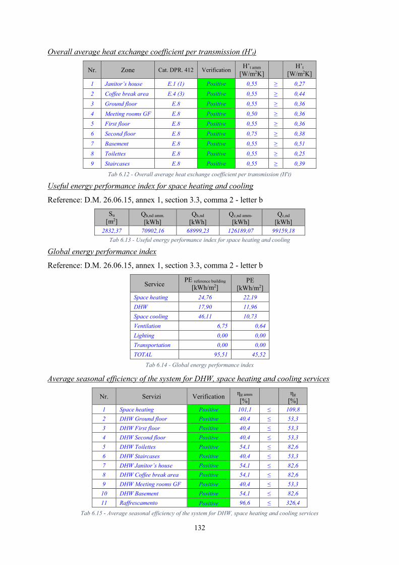
132
Overall average heat exchange coefficient per transmission (H't)
Nr. Zone Cat. DPR. 412 Verification H’t amm
[W/m2K]
H’t
[W/m2K]
1 Janitor’s house E.1 (1) Positive 0,55 ≥ 0,27
2 Coffee break area E.4 (3) Positive 0,55 ≥ 0,44
3 Ground floor E.8 Positive 0,55 ≥ 0,36
4 Meeting rooms GF E.8 Positive 0,50 ≥ 0,36
5 First floor E.8 Positive 0,55 ≥ 0,36
6 Second floor E.8 Positive 0,75 ≥ 0,38
7 Basement E.8 Positive 0,55 ≥ 0,51
8 Toilettes E.8 Positive 0,55 ≥ 0,25
9 Staircases E.8 Positive 0,55 ≥ 0,39
Tab 6.12 - Overall average heat exchange coefficient per transmission (H't)
Useful energy performance index for space heating and cooling
Reference: D.M. 26.06.15, annex 1, section 3.3, comma 2 - letter b
Su
[m2] Qh,nd amm.
[kWh]
Qh,nd
[kWh]
Qc,nd amm.
[kWh]
Qc,nd
[kWh]
2832,37 70902,16 68999,23 126189,07 99159,18
Tab 6.13 - Useful energy performance index for space heating and cooling
Global energy performance index
Reference: D.M. 26.06.15, annex 1, section 3.3, comma 2 - letter b
Service PE reference building
[kWh/m2] PE
[kWh/m2]
Space heating 24,76 22,19
DHW 17,90 11,96
Space cooling 46,11 10,73
Ventilation 6,75 0,64
Lighting 0,00 0,00
Transportation 0,00 0,00
TOTAL 95,51 45,52
Tab 6.14 - Global energy performance index
Average seasonal efficiency of the system for DHW, space heating and cooling services
Nr. Servizi Verification ηg amm
[%]
ηg
[%]
1 Space heating Positive 101,1 ≤ 109,8
2 DHW Ground floor Positive 40,4 ≤ 53,3
3 DHW First floor Positive 40,4 ≤ 53,3
4 DHW Second floor Positive 40,4 ≤ 53,3
5 DHW Toilettes Positive 54,1 ≤ 82,6
6 DHW Staircases Positive 40,4 ≤ 53,3
7 DHW Janitor’s house Positive 54,1 ≤ 82,6
8 DHW Coffee break area Positive 54,1 ≤ 82,6
9 DHW Meeting rooms GF Positive 40,4 ≤ 53,3
10 DHW Basement Positive 54,1 ≤ 82,6
11 Raffrescamento Positive 96,6 ≤ 326,4
Tab 6.15 - Average seasonal efficiency of the system for DHW, space heating and cooling services

133
6.7 Conclusion
Nearly Zero-Energy buildings represent the future reference standard for buildings. In Italy,
requirements for a building to be classified as NZEB have been defined, incentive schemes for
the promotion of their realization are in progress and people are becoming more aware of the
issue. That’s the case of SIGIT, which decided to move its headquarters to an old abandoned
building to turn into the Innovation Square Center and to become a NZEB. In order to do so, a
deep renovation that involved building components and HVAC system was needed.
Two approaches have been followed to estimate the quality of the new combined configuration
of building envelope and conditioning system in terms of energy performances: the quasi-
steady state approach, through the use of Edilclima software (EC700 and EC701 modules), and
the dynamic modelling by the adoption of DesignBuilder program (which uses EnergyPlus as
computational engine). These two ways of evaluating the size of the plant and the energy
performances of the whole building have different basis. It was observed that while the sizing
of the heating system may be similar, the sizing of the cooling system and the assessment of
the energy consumption may be different starting with the standard pre-settings of each
software. In order to evaluate if closer results could be reached, a reiterative procedure was
adopted. Some input data have been defined starting from one model and then entered in the
other and viceversa, with the leading idea to make the two models as equivalent as possible.
Some parameters were easily input (such as stratigraphies of building components and thermal
zones) while other needed more attention. In particular, the definition of internal gains and
ventilation loads took more steps to be achieved: starting from credible values, inconsistent
results came out, so the models have been constantly updated to guarantee coherence between
them. Unfortunately, not all the parameters can be controlled by the user since softwares
automatically deal with them. This leads to differences in the results, some of which more
significative than others. From the results of the DesignBuilder simulation and the Edliclima
simulation, it’s possible to make different kind of conclusions.
Regarding the two programs and consequently the approaches they use, it possible to state that:
- Ediclima overestimates space cooling power, since the value obtained was quite distant from
the one evaluated by DesignBuilder. The space heating powers calculated with both
programs instead were similar;
- When input data can be controlled and set in a coherent way, results matches. That has been
demonstrated by the values of energy losses by ventilation and internal heat gains: in these
cases, the parameters that determine the evaluation of these quantities (internal gains density

134
per zone and ventilation air flowrates) can be manually entered in both softwares and it had
been possible to show the impact that they have on the final energy performance of the model
- When input data cannot be easily controlled by the user (climatic data, solar gains) or cannot
be completely defined (black box), differences in the two computational methods become
evident. That was noticeable from the results in terms of solar heat gains and energy losses
by transmission, which in Edliclima turned out to be higher than in DesignBuilder;
- DesignBuilder allows to input a great variety of HVAC systems, internal loads, schedules,
but requires a deep knowledge of the software to handle all this. On the other hand, Edilclima
has a simpler interface, but input options are reduced. This is comprehensible since Edilclima
was created as a program for the issuance of technical reports and energy performance
certificates of buildings.
For what concerns the building in analysis, it can be affirmed that it is designed to be NZEB
since both the HVAC system (which includes a geothermal air-to-air heat pump fed by
electricity and a photovoltaic plant) and the structure are compliant with normative
requirements: the HVAC system provides for the necessary coverage from renewable sources
and for efficiency values; the structure is well designed in order to guarantee acceptable values
of thermal transmittances per components and global heat transfer coefficient. The possibility
to adjustthe Edilclima model with the data coming from DesignBuilder was deepened during
this study. In this sense, it was showed that defining some parameters, ignoring the
recommended values, might reduce the rough initial approximations of the quasi-steady state
model and make the energy balances more similar to those returned by the dynamic energy
mode. Dynamic simulation of one thermal bridge was also carried out by Therm 7.6, so that the
absence of mould and condensation formation has been demonstrated.
In conclusion, there is not a correct and a wrong method to make power and energy calculations,
since both quasi-steady state and dynamic approaches are based on physical equations and
approximations. The dynamic method can get closer to reality since it has more degrees of
freedom to adapt to the real situation, but it requires a deep knowledge of the structure of the
program and of the significance of each parameter. On the other hand, Edilclima performs more
basic evaluations, but allows to get an acceptable result with a small effort. The combined use
of the two softwares can be the best solution to make energy evaluations: Edilclima can be used
to initially give an order of magnitude of physical quantities and recommended values for
compliance, and then DesignBuilder can come up beside and allow to adjust the size of the
plant on the basis of more realistic operation conditions and of larger variety of possible
technologies to be adopted.

135
References
[1] Ministero dello Sviluppo Economico, Ministero dell’Ambiente e della Tutela del
Territorio e del Mare (2017). SEN 2017 – Strategia energetica nazionale.
[2] European Parliament and Council (18.05.2010). Directive 2010/31/EU on the energy
performance of buildings (recast). Official Journal of the European Union.
[3] Delia D'Agostino, Paolo Zangheri, Barbara Cuniberti, Daniele Paci, Paolo Bertoldi.
(2016). Synthesis Report on the National Plans for Nearly Zero Energy Buildings
(NZEBs) - Progress of Member States towards NZEBs.
[4] European Parliament and Council (30.05.2018). Directive (EU) 2018/844 amending
Directive 2010/31/EU on the energy performance of buildings and Directive 2012/27/EU
on energy efficiency. Official Journal of the European Union.
[5] Jaap Hogeling, Anita Derjanecz (2018). The 2nd recast of the Energy Performance of
Buildings Directive (EPBD). REHVA Journal – April 2018.
[6] (2017) Italian Energy Efficiency Action Plan.
[7] SIGIT (2018). Concorso Innovation Square Center – Bando di concorso
[8] SIGIT (2018). Concorso Innovation Square Center – Documento preliminare alla
progettazione.
[9] EDILCLIMA Engineering & Software (2017). EC700 Calcolo prestazioni energetiche
degli edifici, EC701 Progetto e verifiche edificio-impianto, EC705 Attestato energetico,
EC709 Ponti termici - Manuale d’uso.
[10] CTI - Comitato Termotecnico Italiano (2014). Specifica tecnica UNI/TS 11300-1:2014
[11] CTI - Comitato Termotecnico Italiano (2014). Specifica tecnica UNI/TS 11300-2:2014
[12] CTI - Comitato Termotecnico Italiano (2010). Specifica tecnica UNI/TS 11300-3:2010
136
[13] CTI - Comitato Termotecnico Italiano (2016). Specifica tecnica UNI/TS 11300-4:2016
[14] Diego Ibarra, Christoph Reinhart (2009). Building Performance Simulation for Designers
DesignBuilder // EnergyPlus – Tutorial #1. Harvard Graduate School of Design.
[15] Marco Filippi, Enrico Fabrizio (2017). Dynamic simulation of buildings: EnergyPlus
[16] DesignBuilder Software (2018). DesignBuilder v5 - Compliance With ANSI/ASHRAE/
ACCA Standard 183-2007
[17] Windows and Daylighting Group from Building Technologies Department -
Environmental Energy Technologies Division of Ernest Orlando Lawrence Berkeley
National Laboratory (1998). THERM 2.0 for analyzing two-dimensional heat transfer
through building products
[18] Livio Mazzarella (2011). Ponti termici ed efficienza energetica - Abaco dei ponti termici
[19] CTI - Comitato Termotecnico Italiano (2001). Norma Italiana UNI EN ISO 14683-2001
[20] Riccardo Farina (2016). Il calcolo dei ponti termici alla luce della attuale normativa in
tema di prestazioni energetiche degli edifici.

137
Acknowledgments
Dopo anni di studio, questo atteso giorno è arrivato. Volge al termine un percorso che mi ha
accresciuta personalmente e professionalmente, portando nuove consapevolezze e aspirazioni.
Vorrei spendere qualche parola di ringraziamento nei confronti di tutte le persone che mi hanno
sostenuta e accompagnata fino a qui.
Desidero innanzitutto ringraziare i miei relatori, il Prof. Marco Carlo Masoero per la
disponibilità dimostratami durante il periodo della scrittura della presente tesi, e la Dott.ssa
Laura Rietto per l’aiuto che ha saputo darmi, per la pazienza e per la competenza con cui mi ha
indirizzato nelle occasioni di dubbio.
Inoltre, vorrei ringraziare il team di ingegneri della Ferplant s.r.l per avermi accolto e formato,
in particolare il mio tutor aziendale, l’Ing. Giovanni Cassano per avermi dato l’opportunità di
introdurmi in una realtà professionale e collaborativa e per la fiducia dimostratami, e l’Ing.
Marta Garrone per la grande disponibilità e l’aiuto forniti durante il percorso di tirocinio e di
stesura della tesi.
Un ringraziamento speciale va a tutta la mia famiglia, da sempre punto di riferimento per me.
In particolare, ringrazio i miei genitori, Massimo e Manuela, che mi hanno sempre sostenuto
con il loro affetto e la loro saggezza, e mio fratello Marco per i numerosissimi consigli fornitimi
durante tutti questi anni e l’immenso supporto da sempre dimostratomi: se sono arrivata fin qui
è anche merito suo. Ringrazio inoltre mia nonna Adriana per le parole dolci e di conforto sempre
spese per me, i miei zii e mia cugina Stefania.
Desidero ringraziare Andrea per la sua vicinanza e il suo sostegno, per la fiducia da sempre
dimostratami e per l’amore che mi dà ogni giorno.
Infine, ringrazio tutti coloro che hanno condiviso con me momenti di gioia e di sconforto e che,
vicini o lontani, ci sono sempre stati. In particolare, ringrazio le mie amiche Giulia, Martina,
Laura, Sara e Cristina, per avermi sempre incoraggiata; le mie coinquiline, che in questa
esperienza torinese non mi hanno mai fatto sentire sola; i miei colleghi, in particolare Federica
che è stata la mia compagna di studio e di disavventure in questi anni al Politecnico; gli amici
“lucchesi” e “torinesi” per tutti i momenti di spensieratezza che hanno allietato questo lungo
percorso.
Grazie a tutti.
In questo giorno importante, un pensiero va ai miei nonni Gladys e Piero, che hanno sempre
creduto e investito in me, sperando oggi, come ieri e domani, di essere il loro orgoglio.