Embed Size (px)
Citation preview
POLITECNICO DI MILANO
Facoltà di Ingegneria Industriale
Corso di Laurea Magistrale in Ingegneria Aeronautica
Free-form methodology for aero-structural optimization of wind turbine blades.
Relatore: Prof. Carlo Luigi Bottasso
Co-relatore: Prof. Alessandro Croce
Tesi di Laurea di:
Luca SARTORI Matr. 763764
Anno Accademico 2012 - 2013

Acknowledgements
During the development of this work, I enjoyed the support and the encourage-ment of several people, and I feel indebted with them. First of all, I want toreward the sta of PoliWind research unit at Politecnico di Milano, and espe-cially prof. C. L. Bottasso, prof. A. Croce and F. Gualdoni, for their constantsupport and their precious advice. On the Dutch shore, I want to express mygratitude to Dr. F. Grasso, who attended the uneasy task of being my supervisorat ECN, and to my colleagues from WET unit, with a special thanks to Ms.O.Ceyhan and Mr. J.M.Peeringa. My gratitude goes also to ECN/NRG interns,together with my best wishes for a bright future. Among the others, I want toacknowledge Prof. André Tits, from the University of Maryland, and Dr. B.Jonkman from NREL. A special thanks goes to Dr. J.P. Blasques, from Risø-DTU Denmark, for the constant and enlightning support for what concerns thefunctioning of BECAS.

Abstract
The design of wind turbine blades is a multi-disciplinary task, which requires todeal with multiple objectives and constraints, often in conict with one another.Concerning the aerodynamic design of the blade, current strategies require thatthe characteristics of airfoils are selected at the beginning of the process, usuallyunder genuine two-dimensional considerentions. Subsequently, the shape and thestructural properties of the blade are determined by an optimization process,which allows to maximize the blade performances in a direction which fullls aset of active constraints. Considering that the initial choice of the airfoils caninuence the nal design in a substantial manner, this procedure implies somedegree of uncertainty. Since the airfoils are considered frozen through the entiredesign process, this poses relevant limits which prevent a full exploration of thedesign space. This work investigates an innovative free-form approach for theaero-structural design of rotor blades. This method includes the airol shapesdirectly in the optimization process, in order to perform a simultaneous opti-mization of traditional design variables like chord, twist and structural elementstogether with the various airfoils along the blade. As a consequence, a higherlevel of sensitivity is expected, as much as an improved ability to explore the de-sign domain. Since the airfoil shapes are automatically tailored to the evolutionof the blade, this should result in a lower inuence of the initial choice on thenal conguration, leading to better performances of the blade and, eventually,of the entire wind turbine.
Keywords: Wind energy, blade optimization, airfoil design, aero-structuralanalysis, multi-disciplinary approach.

Riassunto
Intoduzione
L'idea di questo lavoro parte da alcune considerazioni riguardo lo stato dell'artenell'ottimizzazione di pale eoliche. In particolare, per quanto riguarda il progettoaerodinamico, la pratica corrente consiste nello scegliere un set di proli alariche vengono poi assegnati alla pala. Successivamente, il design globale della palaviene svolto per mezzo di una procedura di ottimizzazione vincolata che consentedi ottenere un design ottimo in termini di alcune variabili di progetto, che tipica-mente includono corda e twist della pala, così come variabili legate alla strutturadella pala. Il fatto che i vari proli non cambino durante l'ottimizzazione, ponedei seri limiti sulla reale ecacia dell'ottimizzazione, in quanto restringe signi-cativamente il dominio di ricerca e costringe il design della pala in una direzioneche dipende fortemente dai proli scelti inizialmente.Questo lavoro si propone di studiare le potenzialità di una metodologia di ottimiz-zazione free-form, in cui le forme dei singoli proli siano lasciate libere di variare,come ogni altra variabile interessata dall'ottimizzazione. Lo scopo del lavoro èlo sviluppo di un algoritmo di ottimizzazione che consenta il design simultaneodi pala (sia aerodinamicamente che dal punto di vista strutturale) e proli. Perlo sviluppo del programma, si è scelto di adarsi a modelli matematici general-mente semplici, in modo da non mantenere lo sforzo computazionale entro limitiaccettabili, ma allo stesso tempo si è posta particolare attenzione nel rispettare,seppur in forma semplicata, i vincoli progettuali che determinano normalmenteil design della pala. I risultati attesi sono:
• Una maggiore sensibilità della procedura di ottimizzazione che, potendoadattare liberamente i proli al resto della pala dovrebbe garantire miglioriperformance della soluzione nale.
• Una minor responsabilità del designer nella scelta dei proli iniziali.
Metodologia
per la risoluzione numerica del problema di ottimizzazione, questo lavoro imp-iega un solutore di tipo SQP (Sequential Quadratic Programming) basato su un
viii
metodo a gradiente. Il design evolve in modo da massimizzare in modo iterativouna certa cifra di merito, sotto l'azione di vincoli imposti dall'utente. In partico-lare, come molti lavori nel campo dell'energia eolica, la cifra di merito adottataè il costo dell'energia, che rappresenta la grandezza migliore da minimizzare, inquanto è capace di tenre in considerazione tutti i diversi aspetti della vita opera-tiva della macchina. I vincoli che vengono imposti anché la soluzione rimangasicamente accettabile, riguardano essenzialmente la struttura della pala, in par-ticolare:
• La prima frequenza di appeggio dev'essere maggiore della frequenza nat-urale 3P (comunemente chiamata tre-per-giro).
• Lo sforzo nei singoli elementi strutturali deve mantenersi inferiore a unvalore massimo ammissibile.
E' importante notare che tali vincoli, per quanto generali, sono in grado di ripro-durre vincoli progettuali realmente applicati nel design di pale eoliche di notevolidimensioni.Per quanto riguarda la simulazione della pala, l'algoritmo è diviso in tre sotto-problemi principali, ognuno dei quali agisce su un aspetto fondamentale del designglobale:
• Analisi aerodinamica 2D. La stima delle proprietà aerodinamiche deivari proli dev'essere svolta ad ogni iterata. All'interno del programma,ogni prolo lungo la pala viene prima generato attraverso curve di tipoBézier, e poi analizzato con XFOIL in modo da ottenere dati sulla portanza,resistenza e sul momento in un range di angoli ±20circ. Tali dati vengonopoi estesi all'intero range ±180circ mediante il modello di estrapolazione diViterna-Corrigan.
• Analisi aerodinamica 3D. Il comportamento aerodinamico della pala ècalcolato mediante la teoria dell'elemento di pala (BEM) unita a una dis-tribuzione delle proprietà dei proli ottenute al punto precedente. Il modellodi vento è molto semplice, stazionario e uniforme, e l'output principale diquesta simulazione è l'energia prodotta annualmente (AEP).
• Analisi strutturale. Da un punto di vista strutturale, la pala è rappresen-tata con un modello di pala 1D associato a proprietà di massa e rigidezzain un numero arbitrario di sezioni. Queste ultime sono ottenute medianteanalisi a Elementi Finiti superciali, che viene svolta su ogni sezione inesame. In questo modo, anche gli sforzi locali nei vari elementi vengonovericati. Attraverso il modello 1D, a sua volta discretizzato in ElementiFiniti, è possibile calcolare le frequenze della pala e assicurare il soddisfaci-mento anche del vincolo sulla frequenza.
ix
Il calcolo della cifra di merito viene poi svolto prendendo come input l'energiaprodotta e il peso della pala, che determinano sostanzialmente il costo naledell'energia. Il modello di costo adottato è molto ranato e permette di consid-erare non solo i costi direttamente legati alla pala, ma anche all'intero impianto.
Risultati
L'algoritmo per la metodologia free-form è stato testato pale di diverse dimen-sioni. In questo lavoro vengono proposti due casi, entrambi basati su macchinereali e progettate con criteri di ottimizzazione tradizionali. La prima pala è unatipica macchina da 2MW, caratterizzata da una pala di 45 metri, a cui sonostati assegnati cinque diversi proli 'attivi', cioè integrati nell'ottimizzazione. Ilsecondo caso è una pala da 10MW, progettata presso la Technical Universityof Denmark e adottata come reference nel contesto del consorzio INNWIND. Inentrambi i casi, i risultati dimostrano una buona capacità dell'ottimizzatore digestire il design della pala, in particolare per quel che riguarda lo sviluppo deiproli, oggetto di questa tesi. E' interessante notare come proli sistemati inzone diverse della pala subiscano percorsi di ottimizzazione diversi, e si riscontrauna certa coerenza con la realtà progettuale e manifatturiera delle pale eoliche.in particolare, proli posti vicino alla radice della pala tendono a ridurre il pro-prio spessore, per ridurre il peso, ma al contempo ad aumentare lo spessore albordo di uscita (diventando cioè proli atback). Ciò viene fatto autonoma-mente dall'ottimizzatore, in modo da compensare la perdita di rigidezza ession-ale causata dalla riduzione di spessore. Proli cosiddetti mid-span, ovvero nelmezzo della pala, presentano invece un design che favorisce l'aerodinamica. ingenere, presentano uno spessore simile ai proli di partenza ma una curvaturadecisamente superiore, in modo da produrre più portanza e migliorare l'ecienza.Si nota anche come l'introduzione di carichi superiori venga generalmente com-pensata dall'ottimizzatore attraverso altre variabili. proli di estremità, invece,presentano generalmente una geomteria intermedia, con uno spessore molto ri-dotto rispetto a quelli iniziale e una curvatura aumentata di poco, in modo danon introdurre carichi troppo alti che andrebbero a contribuire signicamente almomento ettente in radice. Interessante notare anche come il design della primapala (2MW) sia dominato dal vincolo di frequenza, mentre il desing della secondapala è dominato da considerazioni di sforzo.
Conclusioni e Sviluppi Futuri
Alla luce delle prove svolte, è possibile aermare che l'obiettivo della tesi è statoraggiunto. In particolar modo, è incoraggiante il fatto che l'ottimizzatore sia ingrado di operare dei miglioramenti anche quando la pala di partenza presenta
x
già un design molto buono. Un'altro punto soddisfacente riguarda la capacitàdell'algoritmo di gestire una gran quantità di variabili di progetto, molto diversetra loro, in modo coerente de ecace. Specialmente per quello che riguarda iproli, è interessante vedere come vincoli di natura molto generale abbiano inrealtà eetti locali motlo importante sul design del singolo prolo.Dal momento che lo scopo di questa tesi è uno studio preliminare, si propongonoalcuni spunti per eventuali studi futuri. In particolar modo:
• Sostituire XFOIL con un solutore numerico più accurato, in modo da avereuna migliore risoluzione della regione di stallo
• Migliorare l'accuratezza della parte strutturale, in particolare attraversoun miglior dettaglio nella descrizione della sezione di pala. Futuri sviluppidel codice dovrebbero permettere il dimensionamento di tutti gli elementiprincipali della struttura.
• Testare il codice con modelli più accurati, in modo da vericarne il com-portamento anche di fronte a vincoli di buckling, o di fatica.
Contents
List of Figures xiv
List of Tables xv
1 Introduction 1
1.1 Scope and methodology of this work . . . . . . . . . . . . . . . . 11.2 State of Art . . . . . . . . . . . . . . . . . . . . . . . . . . . . . . 5
1.2.1 Blade Optimization Tool . . . . . . . . . . . . . . . . . . . 51.2.2 Harp_Opt . . . . . . . . . . . . . . . . . . . . . . . . . . . 61.2.3 Cp-Max . . . . . . . . . . . . . . . . . . . . . . . . . . . . 7
1.3 Considerations about the state of art . . . . . . . . . . . . . . . . 8
2 General Algorithm Description 9
2.1 The Optimization Problem . . . . . . . . . . . . . . . . . . . . . 92.1.1 Sequential Quadratic Programming . . . . . . . . . . . . . 102.1.2 Modied-SQP for reduction of the computational time . . 12
2.2 A multi-disciplinary approach . . . . . . . . . . . . . . . . . . . . 122.3 Project Road-Map . . . . . . . . . . . . . . . . . . . . . . . . . . 17
3 Mathematical Models 19
3.1 Two dimensional aerodynamics . . . . . . . . . . . . . . . . . . . 193.1.1 Airfoils description . . . . . . . . . . . . . . . . . . . . . . 193.1.2 Numerical computation of airfoil data . . . . . . . . . . . . 22
3.2 Three dimensional aerodynamics . . . . . . . . . . . . . . . . . . 243.2.1 Blade description . . . . . . . . . . . . . . . . . . . . . . . 243.2.2 AEP computation . . . . . . . . . . . . . . . . . . . . . . . 27
3.3 Structural analysis . . . . . . . . . . . . . . . . . . . . . . . . . . 303.3.1 Description of the blade section . . . . . . . . . . . . . . . 313.3.2 Finite Elements Methods for structural analysis . . . . . . 333.3.3 Materials . . . . . . . . . . . . . . . . . . . . . . . . . . . 36
4 Case Studies 39
4.1 Reference 2 MW wind turbine . . . . . . . . . . . . . . . . . . . . 39

xii CONTENTS
4.1.1 Optimization set-up . . . . . . . . . . . . . . . . . . . . . 404.1.2 Results . . . . . . . . . . . . . . . . . . . . . . . . . . . . . 43
4.2 DTU-10MW wind turbine . . . . . . . . . . . . . . . . . . . . . . 544.2.1 Optimization set-up . . . . . . . . . . . . . . . . . . . . . 584.2.2 Results . . . . . . . . . . . . . . . . . . . . . . . . . . . . . 60
5 Conclusions 71
5.1 Future developments . . . . . . . . . . . . . . . . . . . . . . . . . 72
List of Figures
1.1 Comparison between a) a traditional blade optimization approach and
b) the free-form approach . . . . . . . . . . . . . . . . . . . . . . . 21.2 Integrated aero-structural approach. . . . . . . . . . . . . . . . . . . 41.3 User interface of the Blade Optimization Tool . . . . . . . . . . . . . 51.4 Strain-detection gauges on a typical HARP_Opt section. . . . . . . 61.5 Architecture of Cp-Max. . . . . . . . . . . . . . . . . . . . . . . . 7
2.1 Modied SQP for simultaneous gradient computation. . . . . . . . . . 122.2 Multi-disciplinary approach and design drivers. . . . . . . . . . . . . 132.3 Organization and timeline of the project. . . . . . . . . . . . . . . . . 17
3.1 font=small . . . . . . . . . . . . . . . . . . . . . . . . . . . . . . . 203.2 Airfoil geometry description with the Bézier curves. . . . . . . . . . . 213.3 Geometric constraints for airfoil description. . . . . . . . . . . . . . . 213.4 Comparison between experimental data and viscous XFOIL simulation
for NACA 1412 airfoil. . . . . . . . . . . . . . . . . . . . . . . . . . 233.5 Example of aerodynamic data extended with Viterna-Corrigan model . 243.6 Chord function described by a 6th order Bézier curve. . . . . . . . . . 253.7 Twist function described by a 6th order Bézier curve. . . . . . . . . . 253.8 Interpolation of airfoils. . . . . . . . . . . . . . . . . . . . . . . . . 263.9 Cp-lambda curves. . . . . . . . . . . . . . . . . . . . . . . . . . . . 283.10 Power Curve. . . . . . . . . . . . . . . . . . . . . . . . . . . . . . . 293.11 Weibull distribution. . . . . . . . . . . . . . . . . . . . . . . . . . . 303.12 Stressed shell blade section. . . . . . . . . . . . . . . . . . . . . . . 313.13 Thickness of structural elements. . . . . . . . . . . . . . . . . . . . . 323.14 Structural simulation workow. . . . . . . . . . . . . . . . . . . . . 343.15 Beam discretization into 1D nite elements. . . . . . . . . . . . . . . 343.16 Finite Elements analysis. a) Airfoil geometry pivoting, b) Mesh gener-
ated by AirfMesh and c) typical BECAS output. . . . . . . . . . . . . 353.17 Convergence analysis for Finite Elements Method. . . . . . . . . . . . 363.18 Assignment of the materials. . . . . . . . . . . . . . . . . . . . . . . 37
4.1 REF45-2.0 wind turbine: blade planform and spar cap position. . . . 40
xiv LIST OF FIGURES
4.2 REF45-2.0 wind turbine: thickness of the structural elements. . . . . 424.3 Delft University airfoils for wind turbines. . . . . . . . . . . . . . . . 434.4 REF45-2.0 wind turbine: relative thickness. . . . . . . . . . . . . . . 434.5 Case study 1: time history of the objective function. . . . . . . . . . 454.6 Case study 1: power curve . . . . . . . . . . . . . . . . . . . . . . . 464.7 Case study 1: torque . . . . . . . . . . . . . . . . . . . . . . . . . . 474.8 Case study 1: rotor speed . . . . . . . . . . . . . . . . . . . . . . . 474.9 Case study 1: chord . . . . . . . . . . . . . . . . . . . . . . . . . . 484.10 Case study 1: twist . . . . . . . . . . . . . . . . . . . . . . . . . . 494.11 Case study 1: local aerodynamic eciency . . . . . . . . . . . . . . 494.12 Case study 1: local power coecient . . . . . . . . . . . . . . . . . 504.13 Case study 1: airfoil 1,2 . . . . . . . . . . . . . . . . . . . . . . . . 504.14 Case study 1: airfoil 3 . . . . . . . . . . . . . . . . . . . . . . . . . 514.15 Case study 1: 3D view of the optimal blade, which highlights the ap-
pearence of atback airfoils near the hub. . . . . . . . . . . . . . . . 514.16 Case study 1: airfoil 4 . . . . . . . . . . . . . . . . . . . . . . . . . 534.17 Case study 1: airfoil 5 . . . . . . . . . . . . . . . . . . . . . . . . . 534.18 Case study 1: airfoil 6 . . . . . . . . . . . . . . . . . . . . . . . . . 544.19 Case study 1: airfoil 7 . . . . . . . . . . . . . . . . . . . . . . . . . 544.20 Case study 1: spar cap thickness . . . . . . . . . . . . . . . . . . . 554.21 Case study 1: root bending moment in storm conditions. . . . . . . . 554.22 Case study 1: spar cap normal stress in storm conditions. . . . . . . 564.23 DTU-10MW wind turbine: blade planform and spar cap position. . . 574.24 DTU-1OMW wind turbine: thickness of the structural elements. . . . 574.25 FFA-W3-XX airfoil family. . . . . . . . . . . . . . . . . . . . . . . 584.26 DTU-1OMW wind turbine: relative thickness. . . . . . . . . . . . . 594.27 Case study 2: time history of the objective function. . . . . . . . . . 614.28 Case study 2: power curve . . . . . . . . . . . . . . . . . . . . . . . 634.29 Case study 2: torque . . . . . . . . . . . . . . . . . . . . . . . . . . 634.30 Case study 2: rotor speed . . . . . . . . . . . . . . . . . . . . . . . 644.31 Case study 2: chord . . . . . . . . . . . . . . . . . . . . . . . . . . 644.32 Case study 2: twist . . . . . . . . . . . . . . . . . . . . . . . . . . 654.33 Case study 2: local aerodynamic eciency . . . . . . . . . . . . . . 654.34 Case study 2: local power coecient . . . . . . . . . . . . . . . . . 664.35 Case study 2: airfoil 3 . . . . . . . . . . . . . . . . . . . . . . . . . 664.36 Case study 2: airfoil 5 . . . . . . . . . . . . . . . . . . . . . . . . . 674.37 Case study 2: airfoil 7 . . . . . . . . . . . . . . . . . . . . . . . . . 674.38 Case study 2: spar cap thickness . . . . . . . . . . . . . . . . . . . 684.39 Case study 2: root bending moment in storm conditions. . . . . . . . 684.40 Case study 2: spar cap normal stress in storm conditions. . . . . . . 69
List of Tables
3.1 Example of airfoils distribution along the blade . . . . . . . . . . 26
4.1 REF45-2.0 wind turbine: overall characteristics . . . . . . . . . . 394.2 REF45-2.0 wind turbine: essential blade-span properties . . . . . 414.3 REF45-2.0 wind turbine: Initial airfoils distribution. . . . . . . . . 414.4 REF45-2.0 wind turbine: Materials. . . . . . . . . . . . . . . . . . 444.5 Case study 1: algorithm performances. . . . . . . . . . . . . . . . 444.6 Case study 1: global optimization results. . . . . . . . . . . . . . . 444.7 Case study 1: aerodynamic performances. . . . . . . . . . . . . . 454.8 Case study 1: blade frequencies. . . . . . . . . . . . . . . . . . . . 464.9 DTU-10MW wind turbine: overall characteristics . . . . . . . . . 564.10 DTU-1OMW wind turbine: Initial airfoils distribution. . . . . . . 594.11 DTU-1OMW wind turbine: Materials. . . . . . . . . . . . . . . . 604.12 Case study 2: algorithm performances. . . . . . . . . . . . . . . . 604.13 Case study 2: global optimization results. . . . . . . . . . . . . . . 604.14 Case study 2: aerodynamic performances. . . . . . . . . . . . . . 614.15 Case study 2: blade frequencies. . . . . . . . . . . . . . . . . . . . 62

Chapter 1
Introduction
In the last years the harvesting of wind power for energy production has increaseddramatically, leading to a signicant interest in the development of methodologiesfor the design of the new generation of wind turbines. In this context, the numer-ical optimization techniques can provide a valuable support in the design process,and at present they are largely employed both in the industry and within researchinstitution. Since modern wind turbines are charactherized by large rotor sizesand by a power production in the range of several megawatts, the optimizationof a rotor blade is a complex problem, which must be addressed with a strongmulti-disciplinary approach. A variety of physical phenomena aect the nal de-sign, and several considerations should be made in order to drive the optimizationtowards an optimal solutions which can improve the behavior of the blade. Atthe same time, a set of constraints should be imposed, in order to maintain thedesign within the tracks of a phisically-meaningful solution. As a result, after op-timization a rotor blade must represent the best compromise between conictingrequirements, which involve aerodynamic performances, structural eciency anddynamic response as much as considerations about convenience and economicfeasibility of the project.
1.1 Scope and methodology of this work
The determination of the aerodynamic behaviour of the blade is an essential stepduring the design of a new wind turbine. In the most known algorithms for windturbines optimization, the aerodynamic loads are generally computed by a three-dimensional model, like BEM methods or the lifting line theory, coupled witha span-wise distribution of the airfoil aerodynamic characteristics, typically thelift and drag coecients and the pitching moment. Then, the full aero-structuraloptimization of the blade can be summarized in the following procedure:
• At the beginning of the process, the various airfoils along the blade arechosen. The airfoils can be selected from existing families or new airfoils can
2 Introduction
be designed on purpose, in order to meet the local requirements. Usually,the choice is driven by both aerodynamic and structural considerations.
• A blade optimization is performed, with the required level of detail:
The chord, twist and other relevant properties like precone angle andsweep are determined, in order to maximize the annual energy pro-duction.
The various structural elements are sized under dynamic and aero-elastic considerations, which typically include fatigue, ultimate loadsand buckling in order to comply with international standards.
• The nal blade is tested with high-complexity models, which include allthe operating conditions and the load envelopes, in order to identify andcorrect possible weakspots which persist after optimization.
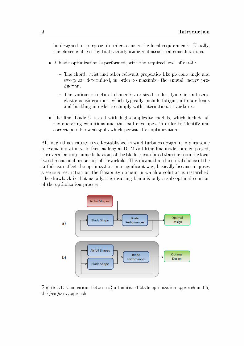
Although this strategy is well-established in wind turbines design, it implies somerelevant limitations. In fact, as long as BEM or lifting line models are employed,the overall aerodynamic behaviour of the blade is estimated starting from the localtwo-dimensional properties of the airfoils. This means that the initial choice of theairfoils can aect the optimization in a signicant way, basically because it posesa serious restriction on the feasibility domain in which a solution is researched.The drawback is that usually the resulting blade is only a sub-optimal solutionof the optimization process.
Figure 1.1: Comparison between a) a traditional blade optimization approach and b)
the free-form approach
1.1 Scope and methodology of this work 3
This work explores an integrated Free-Form methodology for the aero-structuraloptimization of rotor blades. The fundamental idea is to include the airfoil shapesdirectly within the optimization process, so that the local aerodynamic perfor-mances can be adjusted in order to comply with the evolution of the blade design.Under a practical point of view, this means that the shapes of the airfoils alongthe blade are no longer considered frozen, but they are left free to change duringthe analysis, like any other design variable involved in the optimization.Figure 1.1 shows a comparison between the workow of a traditional optimiza-tion algorithm and the free-form methodology investigated in this work. Themain advantage of the free-form approach is that the optimization can aect di-rectly the airfoil shapes, which are no longer treated like a forcing term. Thisshould assure that the optimization is done with a higher level of sensitivity, thusgranting a full exploitation of the domain of feasibility and, consequently, betterperformances of the nal wind turbine. From a practical point of view, the factthat the airfoils are constantly modied during the analysis should decrease theimportance of their initial choice, thus relieving the designers from a delicate apriori choice.
In the following, we illustrate the development of a numerical algorithm for thefree-form optimization of rotor blades, which main goals are:
• to explore the feasibility of this methodology, that is, to verify if standardnumerical optimization techniques can be used to handle the extended setof the design variables without bad-scaling or ill-conditioning problems.
• to test its convenience against the traditional strategies illustrated above.Presumably, the greater level of freedom experienced by the optimizationshould lead to an improved design, even if the starting point is representedby a high-eciency initial blade.
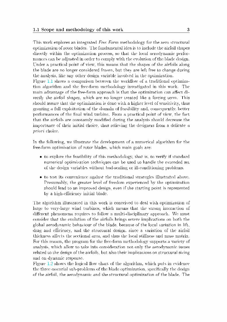
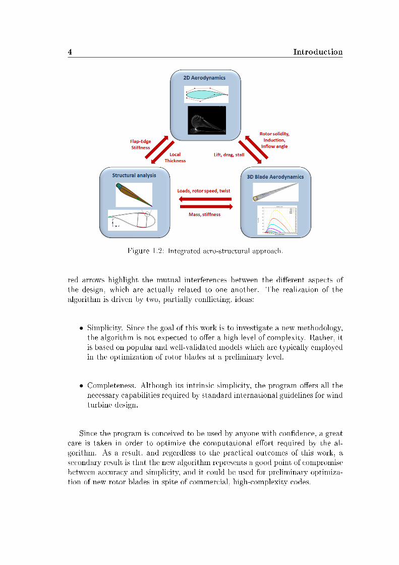
The algorithm illustrated in this work is conceived to deal with optimization oflarge to very-large wind turbines, which means that the strong interaction ofdierent phenomena requires to follow a multi-disciplinary approach. We mustconsider that the evolution of the airfoils brings severe implications on both theglobal aerodynamic behaviour of the blade, because of the local variation in lift,drag and eciency, and the structural design, since a variation of the airfoilthickness aects the sectional area, and thus the local stiness and mass matrix.For this reason, the program for the free-form methodology supports a variety ofanalysis, which allow to take into consideration not only the aerodynamic issuesrelated to the design of the airfoils, but also their implications on structural sizingand on dynamic response.Figure 1.2 shows the logical ow chart of the algorithm, which puts in evidencethe three essential sub-problems of the blade optimization, specically the designof the airfoil, the aerodynamic and the structural optimization of the blade. The
4 Introduction
Figure 1.2: Integrated aero-structural approach.
red arrows highlight the mutual interferences between the dierent aspects ofthe design, which are actually related to one another. The realization of thealgorithm is driven by two, partially conicting, ideas:
• Simplicity. Since the goal of this work is to investigate a new methodology,the algorithm is not expected to oer a high level of complexity. Rather, itis based on popular and well-validated models which are typically employedin the optimization of rotor blades at a preliminary level.
• Completeness. Although its intrinsic simplicity, the program oers all thenecessary capabilities required by standard international guidelines for windturbine design.
Since the program is conceived to be used by anyone with condence, a greatcare is taken in order to optimize the computational eort required by the al-gorithm. As a result, and regerdless to the practical outcomes of this work, asecondary result is that the new algorithm represents a good point of compromisebetween accuracy and simplicity, and it could be used for preliminary optimiza-tion of new rotor blades in spite of commercial, high-complexity codes.
1.2 State of Art 5
1.2 State of Art
The use of numerical optimization in wind turbines design has been extensivelyinvestigated in the literature. However, although a great research eort, thereare still few examples of dedicated algortihms for the systematic solution of theoptimization problem. Here, a quick survey of the most relevant softwares isproposed, in order to cast light on the role of this work in the framework of theavailable material.
1.2.1 Blade Optimization Tool
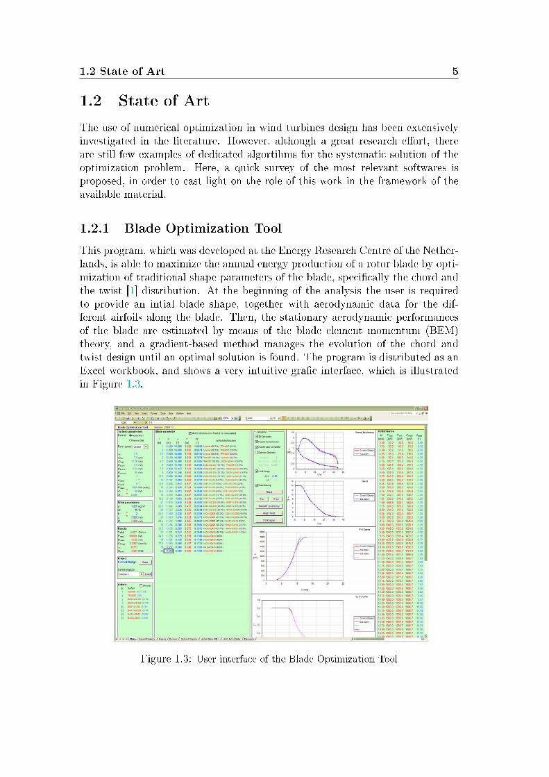
This program, which was developed at the Energy Research Centre of the Nether-lands, is able to maximize the annual energy production of a rotor blade by opti-mization of traditional shape parameters of the blade, specically the chord andthe twist [1] distribution. At the beginning of the analysis the user is requiredto provide an intial blade shape, together with aerodynamic data for the dif-ferent airfoils along the blade. Then, the stationary aerodynamic performancesof the blade are estimated by means of the blade element momentum (BEM)theory, and a gradient-based method manages the evolution of the chord andtwist design until an optimal solution is found. The program is distributed as anExcel workbook, and shows a very intuitive grac interface, which is illustratedin Figure 1.3.
Figure 1.3: User interface of the Blade Optimization Tool
6 Introduction
In order to make the computation of the AEP more accurate, within the BOTenvironment the user has several option in order to personalize the analysis. Inparticular, several corrections can be implemented in the BEM solver in order torene the accuracy, like tip-losses and hub-losses models which can account fortypical three-dimensional phenomena with an acceptable degree of delity. Theuser can also set a maximum chord and a maximum twist in order to bound theoptimization process, and can require to smooth the optimal blade in order tomake it suitable for manifacture. The essential limitation of this tool is that astructural model of the blade is absent, and this requires that the structural designof the blade is carried-out separately. Unfortuntely, since the cross-eects betweenthe aerodynamic and the structural aspects of the design are actually strong, thislimitation could have several implications in the overall design capabilities of thissoftware.
1.2.2 Harp_Opt
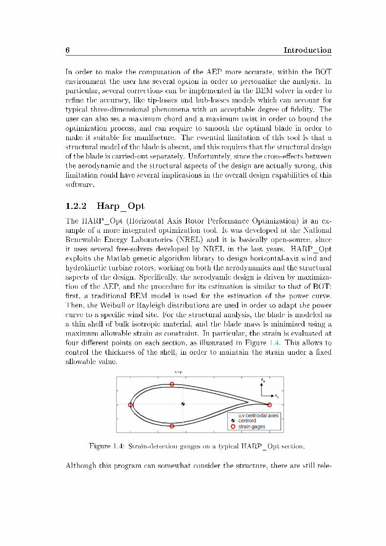
The HARP_Opt (Horizontal Axis Rotor Performance Optimization) is an ex-ample of a more integrated optimization tool. It was developed at the NationalRenewable Energy Laboratories (NREL) and it is basically open-source, sinceit uses several free-solvers developed by NREL in the last years. HARP_Optexploits the Matlab genetic algorithm library to design horizontal-axis wind andhydrokinetic turbine rotors, working on both the aerodynamics and the structuralaspects of the design. Specically, the aerodyamic design is driven by maximiza-tion of the AEP, and the procedure for its estimation is similar to that of BOT:rst, a traditional BEM model is used for the estimation of the power curve.Then, the Weibull or Rayleigh distributions are used in order to adapt the powercurve to a specic wind site. For the structural analysis, the blade is modeled asa thin shell of bulk isotropic material, and the blade mass is minimized using amaximum allowable strain as constraint. In particular, the strain is evaluated atfour dierent points on each section, as illustrated in Figure 1.4. This allows tocontrol the thickness of the shell, in order to maintain the strain under a xedallowable value.
Figure 1.4: Strain-detection gauges on a typical HARP_Opt section.
Although this program can somewhat consider the structure, there are still rele-
1.2 State of Art 7
vant limitations. First, the two problems (aerodynamic and structural) are notmerged in a single integrated optimization process, but they are still consideredas two independent sub-problems. Second, since only the shell is modelled, thedescription of each section is quite elementary, and allows only a verication ofthe structural properties rather than an organized and focused design.
1.2.3 Cp-Max
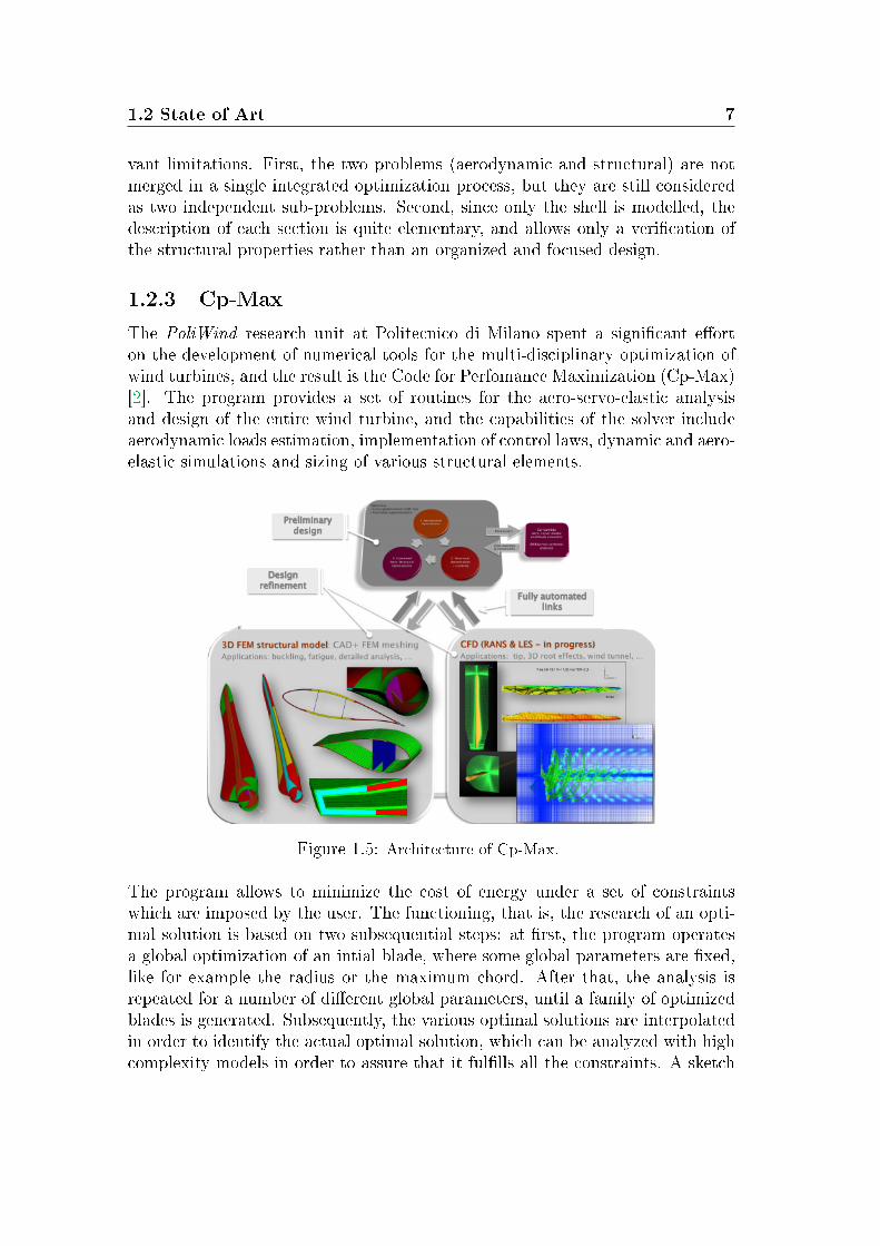
The PoliWind research unit at Politecnico di Milano spent a signicant eorton the development of numerical tools for the multi-disciplinary optimization ofwind turbines, and the result is the Code for Perfomance Maximization (Cp-Max)[2]. The program provides a set of routines for the aero-servo-elastic analysisand design of the entire wind turbine, and the capabilities of the solver includeaerodynamic loads estimation, implementation of control laws, dynamic and aero-elastic simulations and sizing of various structural elements.
Figure 1.5: Architecture of Cp-Max.
The program allows to minimize the cost of energy under a set of constraintswhich are imposed by the user. The functioning, that is, the research of an opti-mal solution is based on two subsequential steps: at rst, the program operatesa global optimization of an intial blade, where some global parameters are xed,like for example the radius or the maximum chord. After that, the analysis isrepeated for a number of dierent global parameters, until a family of optimizedblades is generated. Subsequently, the various optimal solutions are interpolatedin order to identify the actual optimal solution, which can be analyzed with highcomplexity models in order to assure that it fullls all the constraints. A sketch
8 Introduction
of the architecture of the program is provided in Figure 1.5. The advantage ofCp-Max is that it oers a high level of detail in the simulation of the wind turbinefrom the very preliminary stages of design but, on the other hand, it still relieson combined 2D/3D models for the aerodynamic analysis of the blade, that is,the user must still provide data about the various airfoils.
1.3 Considerations about the state of art
The available resources employed for rotor blade optimization oer a variety ofmethodologies and dierent levels of detail. It is reamrakble to notice that atpresent the need for complete aero-structural models is largely accepted but,however, the idea of including the airfoils within the optimiztion process seemsto remain unexplored. In this context, this study can oer a stronger insight ofwhat concerns the capabilities of modern optimization techniques, particularlyabout the strategies which drive the design of wind turbines-dedicated airfoils. Astraditional optimization techniques are somewhat limited by the need to provideairfoils data, the algorithm for the free-form approach can oer a more exibletool and could represent a signicant step towards a truly integrated blade design.From a practical point of view, this program can represent also a reliable, thoughsimple, start point for further more accurate investigations.
This work, and specically the algorithm, has been developed within a joint-project between Politecnico di Milano and the Energy Research Centre of theNetherlands (ECN), and is partially supported by the FP7 INNWIND project.
Chapter 2
General Algorithm Description
This Chapter illustrates the high-level features of the free-form algorithm de-veloped in this work. The scope is to illustrate how the algorithm can addressand manage the optimization of large rotor blades and to identify, among dier-ent strategies, which best suit the needs of this study. First, the formulation ofthe general optimization problem is provided, together with a brief account ofthe available techniques for its numerical solution. The features of the gradient-based SQP methods are also revised, in order to explain which considerationsmake these methods a good choice. It follows a description about the need tosolve the aero-structural blade design problem with a multi-disciplinary approachand, in particular, the choice of the objective function and constraints is discussedextensively, as they play a crucial role in the behaviour of the optimization algo-rithm.
2.1 The Optimization Problem
Optimization is an iterative procedure which is able to nd the point of minimumof a multi-dimensional function while granting, at the same time, that a set ofactive constraints is respected at each iteration. Under a mathematical point ofview, a traditional optimization algorithm can be expressed by the problem:
find : minf(x) (2.1)
so that:
bli ≤ xi ≤ bui
gj(x) ≤ 0 j = 1, ..., ni
hj(x) = 0 j = 1, ..., ne
(2.2)
where x = x1, x2, ..xn is the set of the design variables, f(x) is the objectivefunction. bli and bui represent the boundary values for each design variable xi
10 General Algorithm Description
and dene the searchable design space, while gj and hj are, respectively, a setof inequality constraints and a set of equality constraints for the problem. Theconstraints divide the design space into two domains, the feasible domain, wherethe constraints are satised, and the infeasible domain where at least one ofthe constraints is violated. In most practical problems the minimum is foundon the boundary between the feasible and infeasible domains, that is at a pointwhere gj(x) = 0 for at least one j . In many aerodynamics and wind energyapplications, the use of inequality constraints is of paramount importance, as theunconstrained optimization can evolve towards an unphysical conguration: fora detailed example, the reader can refer to [3]. In the general case, the objectiveand constraint functions can be linear or non-linear and can be explicit or implicitfunctions. This is the case, for example, when numerical techniques are employedto evaluate the objective function or the constraints, as in the Finite ElementsMethods. Although the problem (2.1) is expressed by analitical functions, in themajority of applications the design variables are not required to be continuous,but they are provided in some discrete form.
2.1.1 Sequential Quadratic Programming
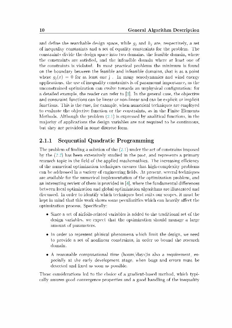
The problem of nding a solution of the (2.1) under the set of constrains imposedby the (2.2) has been extensively studied in the past, and represents a primaryresearch topic in the eld of the applied mathemathics. The increasing eciencyof the numerical optimization techniques ensures that high-complexity problemscan be addressed in a variety of engineering elds. At present, several techniquesare available for the numerical implementation of the optimization problem, andan interesting review of them is provided in [4], where the fundamental dierencesbetween local optimization and global optimization algorithms are illustrated anddiscussed. In order to identify which techniques best suits our scopes, it must bekept in mind that this work shows some peculiarities which can heavily aect theoptimization process. Specically:
• Since a set of airfoils-related variables is added to the traditional set of thedesign variables, we expect that the optimization should manage a largeamount of parameters.
• In order to represent phisical phenomena which limit the design, we needto provide a set of nonlinear constraints, in order to bound the researchdomain.
• A reasonable computational time (hours/days)is also a requirement, es-pecially at the early development stage, when bugs and errors must bedetected and xed as soon as possible.
These considerations led to the choice of a gradient-based method, which typi-cally assures good convergence properties and a good handling of the inequality
2.1 The Optimization Problem 11
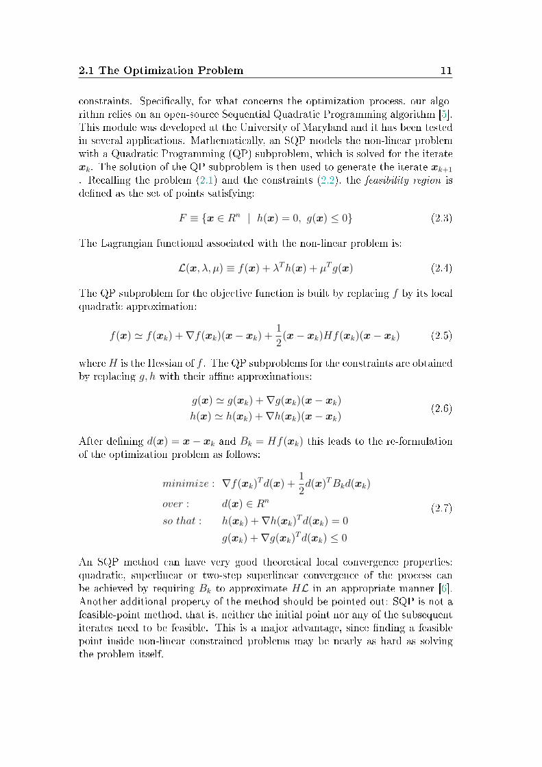
constraints. Specically, for what concerns the optimization process, our algo-rithm relies on an open-source Sequential Quadratic Programming algorithm [5].This module was developed at the University of Maryland and it has been testedin several applications. Mathematically, an SQP models the non-linear problemwith a Quadratic Programming (QP) subproblem, which is solved for the iteratexk. The solution of the QP subproblem is then used to generate the iterate xk+1
. Recalling the problem (2.1) and the constraints (2.2), the feasibility region isdened as the set of points satisfying:
F ≡ x ∈ Rn | h(x) = 0, g(x) ≤ 0 (2.3)
The Lagrangian functional associated with the non-linear problem is:
L(x, λ, µ) ≡ f(x) + λTh(x) + µTg(x) (2.4)
The QP subproblem for the objective function is built by replacing f by its localquadratic approximation:
f(x) ≃ f(xk) +∇f(xk)(x− xk) +1
2(x− xk)Hf(xk)(x− xk) (2.5)
whereH is the Hessian of f . The QP subproblems for the constraints are obtainedby replacing g, h with their ane approximations:
g(x) ≃ g(xk) +∇g(xk)(x− xk)
h(x) ≃ h(xk) +∇h(xk)(x− xk)(2.6)
After dening d(x) = x− xk and Bk = Hf(xk) this leads to the re-formulationof the optimization problem as follows:
minimize : ∇f(xk)Td(x) +
1
2d(x)TBkd(xk)
over : d(x) ∈ Rn
so that : h(xk) +∇h(xk)Td(xk) = 0
g(xk) +∇g(xk)Td(xk) ≤ 0
(2.7)
An SQP method can have very good theoretical local convergence properties:quadratic, superlinear or two-step superlinear convergence of the process canbe achieved by requiring Bk to approximate HL in an appropriate manner [6].Another additional property of the method should be pointed out: SQP is not afeasible-point method, that is, neither the initial point nor any of the subsequentiterates need to be feasible. This is a major advantage, since nding a feasiblepoint inside non-linear constrained problems may be nearly as hard as solvingthe problem itself.
12 General Algorithm Description
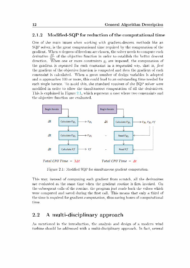
2.1.2 Modied-SQP for reduction of the computational time
One of the main issues when working with gradient-descent methods like anSQP solver, is the great computational time required by the computation of thegradient. When n degrees of freedom are chosen, the solver needs to compute eachderivative ∂f
∂xnof the objective function in order to establish the better descent
direction. When one or more constraints gj are imposed, the computation ofthe gradient is repeated for each constraint in a sequential way, that is, rstthe gradient of the objective function is computed and then the gradient of eachconstraint is calculated. When a great number of design variables is adoptedand n approaches 100 or more, this could lead to an outstanding time needed foreach single iterate. To avoid this, the standard routines of the SQP solver weremodied in order to allow the simultaneous computation of all the derivatives.This is explained in Figure 2.1, which represent a case where two constraints andthe objective function are evaluated.
Figure 2.1: Modied SQP for simultaneous gradient computation.
This way, instead of computing each gradient from scratch, all the derivativesare evaluated at the same time when the gradient routine is rst invoked. Onthe subsequent calls of the routine, the program just reads back the values whichwere computed and saved during the rst call. This means that only a third ofthe time is required for gradient computation, thus saving hours of computationaltime.
2.2 A multi-disciplinary approach
As mentioned in the introduction, the analysis and design of a modern windturbine should be addressed with a multi-disciplinary approach. In fact, several
2.2 A multi-disciplinary approach 13
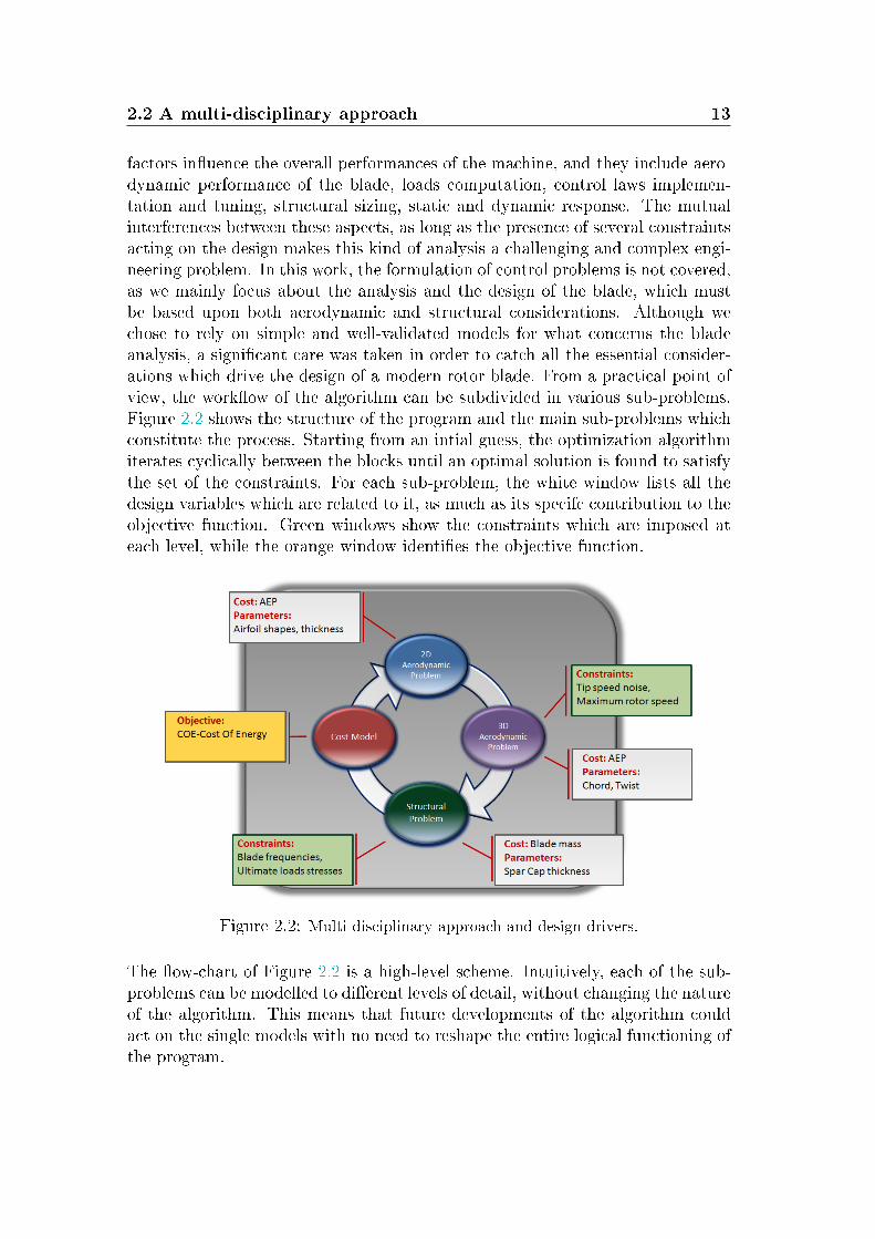
factors inuence the overall performances of the machine, and they include aero-dynamic performance of the blade, loads computation, control laws implemen-tation and tuning, structural sizing, static and dynamic response. The mutualinterferences between these aspects, as long as the presence of several constraintsacting on the design makes this kind of analysis a challenging and complex engi-neering problem. In this work, the formulation of control problems is not covered,as we mainly focus about the analysis and the design of the blade, which mustbe based upon both aerodynamic and structural considerations. Although wechose to rely on simple and well-validated models for what concerns the bladeanalysis, a signicant care was taken in order to catch all the essential consider-ations which drive the design of a modern rotor blade. From a practical point ofview, the workow of the algorithm can be subdivided in various sub-problems.Figure 2.2 shows the structure of the program and the main sub-problems whichconstitute the process. Starting from an intial guess, the optimization algorithmiterates cyclically between the blocks until an optimal solution is found to satisfythe set of the constraints. For each sub-problem, the white window lists all thedesign variables which are related to it, as much as its specifc contribution to theobjective function. Green windows show the constraints which are imposed ateach level, while the orange window identies the objective function.
Figure 2.2: Multi-disciplinary approach and design drivers.
The ow-chart of Figure 2.2 is a high-level scheme. Intuitively, each of the sub-problems can be modelled to dierent levels of detail, without changing the natureof the algorithm. This means that future developments of the algorithm couldact on the single models with no need to reshape the entire logical functioning ofthe program.
14 General Algorithm Description
Objective function
In wind energy optimization, usually the Cost Of Energy, COE is taken as objec-tive function. This is done because, in a global and competitive energy market,the main goal of the wind energy industry is to maintain the costs comparableagainst traditional energy sources. The Cost Model proposed in [7] was devel-oped by the National Renewable Energy Laboratories, NREL. It is based on ascaling model applied to a traditional upwind, three-bladed wind turbine andallows to link the COE to a series of parameters which include rotor radius,blade weight and Annual Energy Production. These can be easily related to tra-ditional design variables used in the optimization, thus obtaining a single andprecise objective function which is capable of taking into account all the aspectsof a multi-disciplinary approach. The most common deinition of the cost ofenergy is:
COE =FCR x ICC
AEPnet
+ AOE (2.8)
where:
• COE = Levelized Cost Of Energy ( $kWh
)
• FCR = Fixed Charge Rate
• ICC = Initial Capital Cost
• AEPnet = Net Annual Energy Production
• AOE = Annual Operating Expenses
From the designer's viewpoint, the advantage of this model is that it allows toevalute the economic impact of specic design strategies, by taking into accountall the aspects of the operational life of the machine. In fact, each of the mem-bers of the equation (2.8) is computed from further contributions which, startingfrom the values of the design variables, can calculate the impact of each singlecomponents to the total cost of energy. For brevity, a detailed description ofthe cost model is not illustrated here, even because a great research eort is stillongoing in order to rene the model and make the estimate of the cost of energymore accurate. Another advantage of this model is that it allows the optimizationto act eectively on all the dierent parameters aecting the cost, that is, theoptimization will pursue an increase in the AEP as much as a decrease in bladeweight, which makes the cost of energy more suitable for optimization purposesthan other traditional objective functions exploited in the past.
2.2 A multi-disciplinary approach 15
Constraints
The choice of the active constraints that should be included in the optimizationprocess is an important step of the algorithm development, especially becausethey should represent a good choice of compromise between simplicity and com-pleteness. The certication of modern wind turbines is regulated by internationalstandards [8],[9] which require to test the machine under a variety of circum-stances, which are summarized in several design load cases, DLC. They includenormal operating conditions, ultimate loads from storm, emergency shutdownand full-turbulent ow simulations. Obviously, an accurate verication of theDLCs requires detailed aero-elastic models coupled with unsteady aerodynamicmodels, as illustrated in the already cited paper [2]. Since this level of detail goesbeyond the scope of this work, in our algorithm we introduce some constraintswhich can be considered as simplied load cases. The scope is to maintain a strictcompliance with the required verications, without the burden of simulations andanalysis required to a commercial software. Specically, the simplied load casestaken into considerations are translated into the two following constraints:
• Operating conditions: the rst apwise frequency must be higher
than the 3P. This is imposed by the relation:
ϵfreq −fflap − f3P
f3P≤ 0 (2.9)
where fflap is the rst apwise frequency of the blade, f3P is the three-per-revolution natural frequency of the blade, and ϵfreq is the desired clearancebetween the two. This constraint poses a lower limit on the rst apwisefrequency of the blade corresponding to the nominal operating conditions.The goal is to avoid the superposition between the blade frequency and the3P, which could result in dangerous resonance phenomena. Since the rstapwise frequncy depends largely on the out-of-plane stiness of the blade,this constraint should regulate the absolute blade thickness and the sizingof the structural elements, especially the spar caps.
• Storm conditions: the maximum stress must be lower than the
admittable stress. This condition is enforced on each blade section, anddrives the sizing of the structural elements so that the optimal blade canwithstand ultimate loads deriving from storm conditions. This can be ex-pressed by the relation:
ϵσ −σadm − σMax
σadm
≤ 0 (2.10)
where σMax = max(σi), that is, the maximum stress detected along theblade. Again, ϵσ is a tolerance that allows the User to set the requireddegree of safety.
16 General Algorithm Description
In addition to these constraints, a limit on the maximum tip speed is imposed.This condition, which concerns the design of onshore wind turbines, derives fromacoustic considerations: as the rotor speed of the wind turbine increases, theaerodynamic and mechanical noise can reach high levels, aecting the surroundingenvironment in a negative manner [10]. This is true especially for megawatt-size machines, which are characterized by great tip velocities. To respect theregulation in force for this class of machines, it is imposed that the tip velocitycan not overcome a certain value, which is usually set equal to 72m
s:
vtipmax ≡ 72m
s
Ωmax =vtipmax
R
(2.11)
From the (2.11), it is possible to notice that this requirement aects the max-imum rotor speed and, in turn, the regulation strategies and the production ofenergy. Dislike (2.10) and (2.9), which are explicitly veried by the optimizer ateach iterate, the tip-speed constraints is implicitly imposed when the regulationtrajectories of the machine are computed.
Design variables
The array of the design variables is dened as the set of the degrees of free-dom, that is, it stores all the parameters which are directly controlled by theoptimization. In order to grant that all the searchable domain is explored, thearray should include several groups of variables, which are related to the dier-ent sub-problems of Figure 2.2. In this work, the design variables must includethe geometrical description of chord and twist, as much as parametes related toan arbitrary number of airfoils. A description of the various structural elementsmust also be included in the set of the design variables. Let x be the array ofthe design variables, it can be considered composed by four families of variablesas follows:
x = [xch xtw xst xaf ] (2.12)
where:
• xch = [x1ch, ..., x
nchch ] includes the nch variables related to the chord descrip-
tion.
• xtw = [x1tw, ..., x
ntwtw ] includes the ntw variables related to the twist descrip-
tion.
• xst = [x1st, ..., x
nstst ] includes the variables related to the thickness of the
structural elements.
2.3 Project Road-Map 17
• xaf = [x1af , ..., x
naf
af ] includes the variables related to the shapes of the air-foils.
the next Chapter illustrates how the design variables are chosen in order to rep-resent the blade shape in a high delity manner.
2.3 Project Road-Map
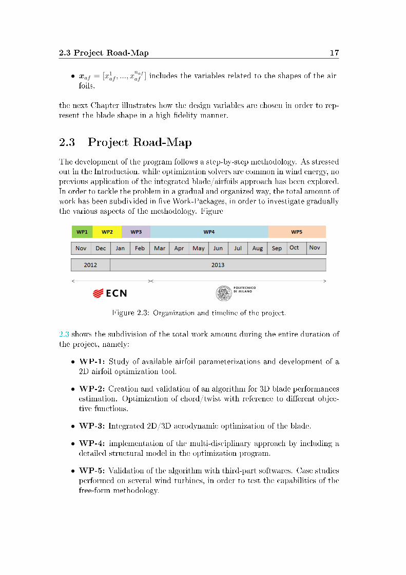
The development of the program follows a step-by-step methodology. As stressedout in the Introduction, while optimization solvers are common in wind energy, noprevious application of the integrated blade/airfoils approach has been explored.In order to tackle the problem in a gradual and organized way, the total amount ofwork has been subdivided in ve Work-Packages, in order to investigate graduallythe various aspects of the methodology. Figure
Figure 2.3: Organization and timeline of the project.
2.3 shows the subdivision of the total work amount during the entire duration ofthe project, namely:
• WP-1: Study of available airfoil parameterizations and development of a2D airfoil optimization tool.
• WP-2: Creation and validation of an algorithm for 3D blade performancesestimation. Optimization of chord/twist with reference to dierent objec-tive functions.
• WP-3: Integrated 2D/3D aerodynamic optimization of the blade.
• WP-4: implementation of the multi-disciplinary approach by including adetailed structural model in the optimization program.
• WP-5: Validation of the algorithm with third-part softwares. Case studiesperformed on several wind turbines, in order to test the capabilities of thefree-form methodology.
18 General Algorithm Description
As illustrated in the picture, WP-1, WP-2 and partially WP-3 were developedat the headquarter of ECN in Petten, the Netherlands, under the supervision ofDr.Grasso. WP-4 and WP-5 were conducted at the Poli-Wind unit at Politecnicodi Milano, under the supervision of Prof. C.L. Bottasso and Prof. A. Croce. Thegoal of this kind of organization was to exploit the great experience gained in thepast years by both ECN and Politecnico in the eld of optimization of Multi-MWclass Wind Turbines.
Chapter 3
Mathematical Models
This Chapter provides a survey of the various mathematical models employedin this work. The presentation is divided in three main sub-problems: the 2Daerodynamic description of the blade, the estimation of the 3D aerodynamiccharacteristics and the structural problem. For each sub-problem, the choice ofthe design variables is discussed, together with the numerical methods adopted forits solution. The scope is to oer a detailed view of the algorithm capabilities,and to understand the hypothesis and assumptions made at each level of theoptimization process.
3.1 Two dimensional aerodynamics
3.1.1 Airfoils description
The representation of the airfoils plays a crucial role within the free-form ap-proach here investigated. The fact that the airfoil shapes are now included asdesign variables adds some complexities to the already tangled problem of bladeoptimization. Let's consider, for example, that in state of art algorithms theairfoil data are often provided from wind tunnel measurements. When the air-foils are unfrozen, like in the free-form approach, the estimation of aerodynamicdata at each iterate must be done by a numerical method which must replace thewind tunnel experiments, possibly with a high level of accuracy. Moreover, asintroduced before, having free airfoil geometries introduces a signicant numberof additional variables in the optimization. It follows that to avoid an unbearablecomputational time, it is fundamental to describe the airfoil shapes through someparameterization.
Bézier curves This theory for curves representation is due to Dr.Pierre Bézier,who rst introduced this formulation inside Renault in 1960. Subsequently, Béziercurves knew a wide expansion, especially in CAD softwares and in the eld of
20 Mathematical Models
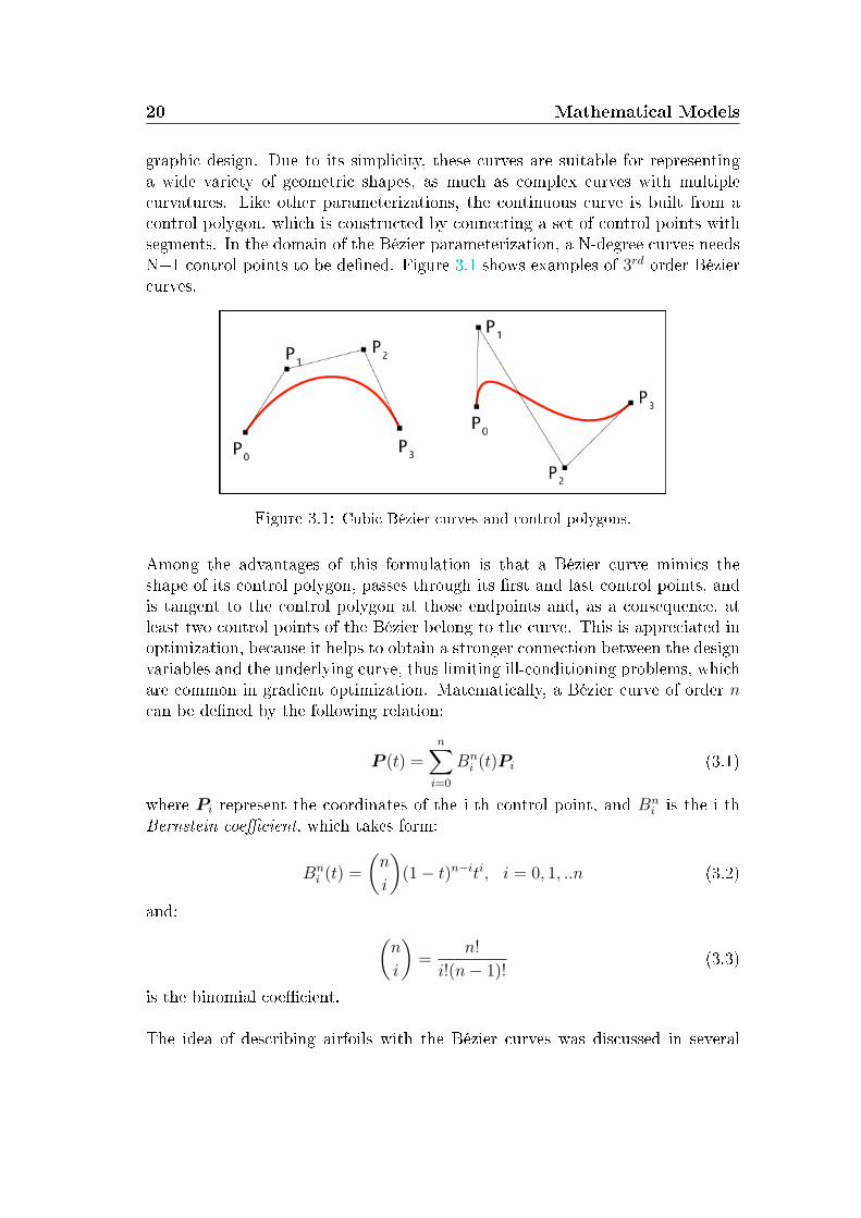
graphic design. Due to its simplicity, these curves are suitable for representinga wide variety of geometric shapes, as much as complex curves with multiplecurvatures. Like other parameterizations, the continuous curve is built from acontrol polygon, which is constructed by connecting a set of control points withsegments. In the domain of the Bézier parameterization, a N-degree curves needsN+1 control points to be dened. Figure 3.1 shows examples of 3rd order Béziercurves.
Figure 3.1: Cubic Bézier curves and control polygons.
Among the advantages of this formulation is that a Bézier curve mimics theshape of its control polygon, passes through its rst and last control points, andis tangent to the control polygon at those endpoints and, as a consequence, atleast two control points of the Bézier belong to the curve. This is appreciated inoptimization, because it helps to obtain a stronger connection between the designvariables and the underlying curve, thus limiting ill-conditioning problems, whichare common in gradient optimization. Matematically, a Bézier curve of order ncan be dened by the following relation:
P (t) =n∑
i=0
Bni (t)Pi (3.1)
where Pi represent the coordinates of the i-th control point, and Bni is the i-th
Bernstein coecient, which takes form:
Bni (t) =
(n
i
)(1− t)n−iti, i = 0, 1, ..n (3.2)
and: (n
i
)=
n!
i!(n− 1)!(3.3)
is the binomial coecient.
The idea of describing airfoils with the Bézier curves was discussed in several
3.1 Two dimensional aerodynamics 21
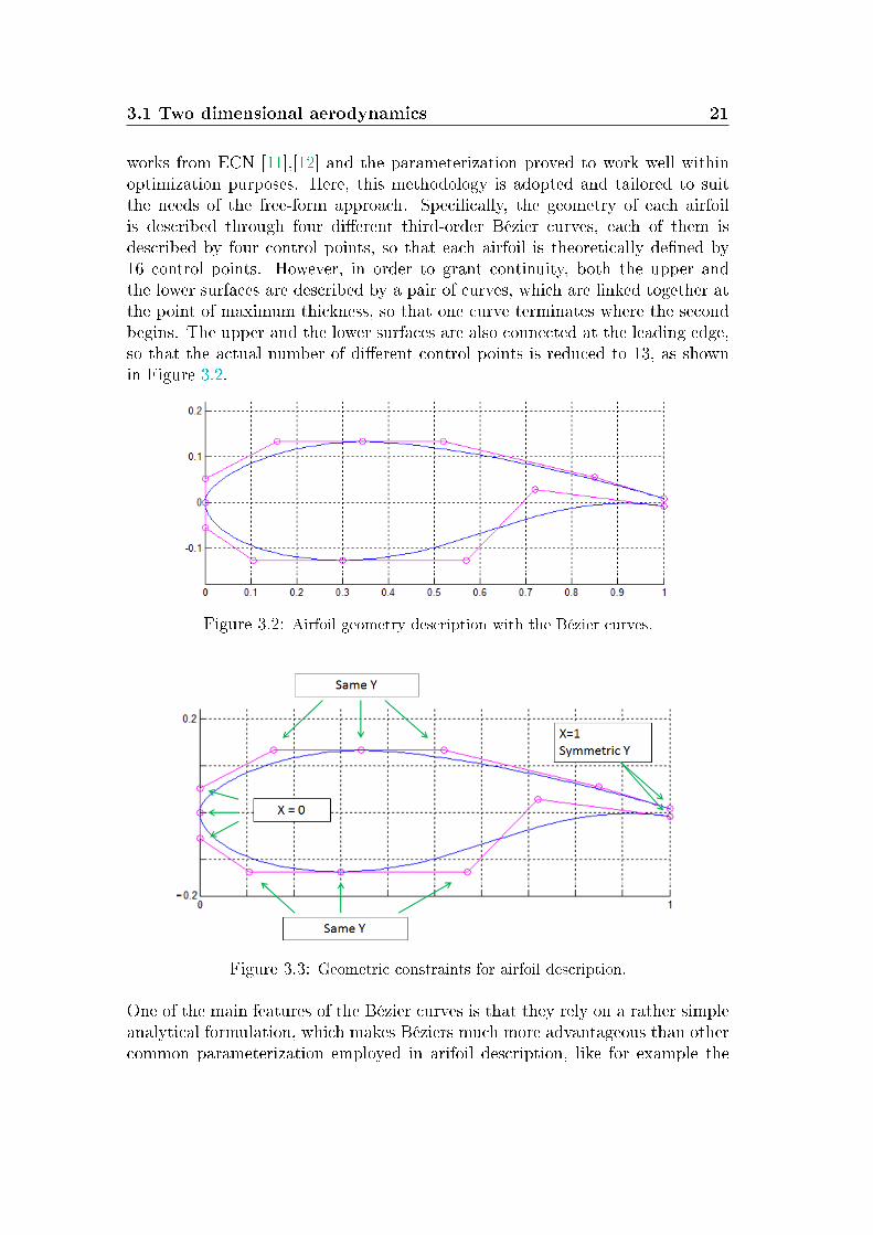
works from ECN [11],[12] and the parameterization proved to work well withinoptimization purposes. Here, this methodology is adopted and tailored to suitthe needs of the free-form approach. Specically, the geometry of each airfoilis described through four dierent third-order Bézier curves, each of them isdescribed by four control points, so that each airfoil is theoretically dened by16 control points. However, in order to grant continuity, both the upper andthe lower surfaces are described by a pair of curves, which are linked together atthe point of maximum thickness, so that one curve terminates where the secondbegins. The upper and the lower surfaces are also connected at the leading edge,so that the actual number of dierent control points is reduced to 13, as shownin Figure 3.2.
Figure 3.2: Airfoil geometry description with the Bézier curves.
Figure 3.3: Geometric constraints for airfoil description.
One of the main features of the Bézier curves is that they rely on a rather simpleanalytical formulation, which makes Béziers much more advantageous than othercommon parameterization employed in arifoil description, like for example the
22 Mathematical Models
PARSEC, which requires highly nonlinear equations to be solved in order toestimate the airfoil shape[13]. At the same time, due to its exibility the Bézierformulation allows a great variety of airfoils to be explored. Within the purposesof this work, for example, it is possible to obtain geometries which are commonlyemployed in modern wind turbines, like atback airfoils and S-tail trailing edge forrear-loading. Obviously, such a broad domain can result in strange airfoil shapesappearing during the optimization. In the worst cases, the two-dimensional solvercan fail to converge, if the geometry is not smooth enough to allow panel methodsto be employed. To avoid this situation, a great care has been taken in order togure out a set of geometric constraints, which are illustrated in Figure 3.3. Thisputs some limits in the freedom enjoyed by each control point, forcing each pairof curves to have the same tangent at the connecting point, in order to guaranteethat all the curves are merged in a regular and smooth way. As it is evidentfrom the gure, this control does not act at the trailing edge, where the upperand the lower surfaces terminate on dierent points, in order to allows atbackairfoils. After accounting for the geometric constraints, the number of necessarydegrees of freedom for describing each airfoil is 15, which assures enough freedomto allow the representation of a wide range of existing airfoils (DU, FFA, Risø)with a high level of delity.
3.1.2 Numerical computation of airfoil data
As outlined in the introduction, typical three-dimensional solvers employed inwind turbines optimization are based on a combined 2D/3D approach. Thismeans that, in order to estimate the three-dimensional aerodynamic performanceof the blade, and thus the energy production, it is necessary to provide informa-tions about the local characteristics of the airfoils, typically the lift, the drag andthe pitching moment for one or several Reynolds numbers. As the airfoils varyduring optimization, it is necessary to provide those values numerically, in theentire range of angles of attack encompassed between ±180. In our algorithm,this is done as follows: at rst, each airfoil is evaluated in the range ±20 withthe popular solver XFOIL [14] then, a numerical implemetation of the Viterna-Corrigan method extends the data collected from XFOIL to the whole range [15].This strategy has been previously adopted for the optimization of wind and tidalturbines dedicated airfoils, as illustrated in [16]. While the details of the modelscan be found in the references, it is our interest here to provide a brief summaryof the capabilities of XFOIL. In particular, the program provides:
• An inviscid formulation, based on a simple linear-vorticity stream functionpanel method, completed with the forcing of the Kutta condition at thetrailing edge
• A Karman-Tsien compressibility correction which allows good compressiblepredictions until the appearence of the sonic conditions
3.1 Two dimensional aerodynamics 23
• A viscous formulation, which relies on a two-equation lagged dissipation BLformulation and a en transition criterion.
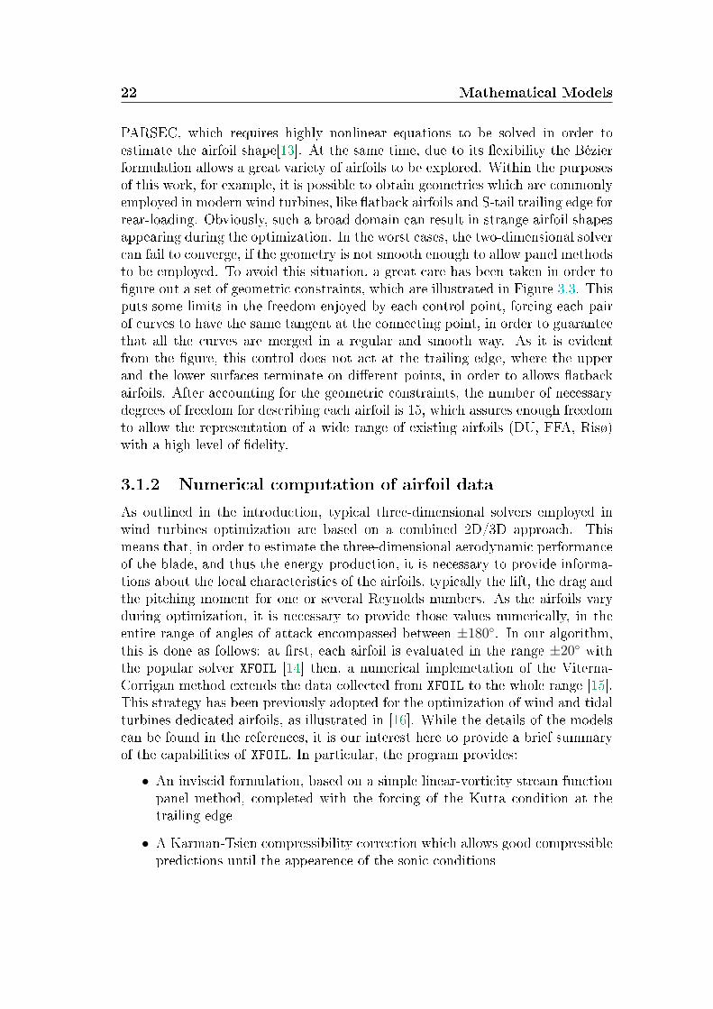
The coupling between inviscid and viscous formulations allows to perform a va-riety of analysis which go further the estimation of lift, drag and moment at acertain angle of attack. However, as stressed out in the documentation, the pro-gram provides reliable results only in the pre-stall region, where a good agreementwith experimental data is usually obtained. In Figure 3.4 wind tunnel data forthe NACA 1412 airfoil are compared against a viscous simulation performed withXFOIL. Both the data series refer to a Reynolds number of 3 millions [17].
Figure 3.4: Comparison between experimental data and viscous XFOIL simulation for
NACA 1412 airfoil.
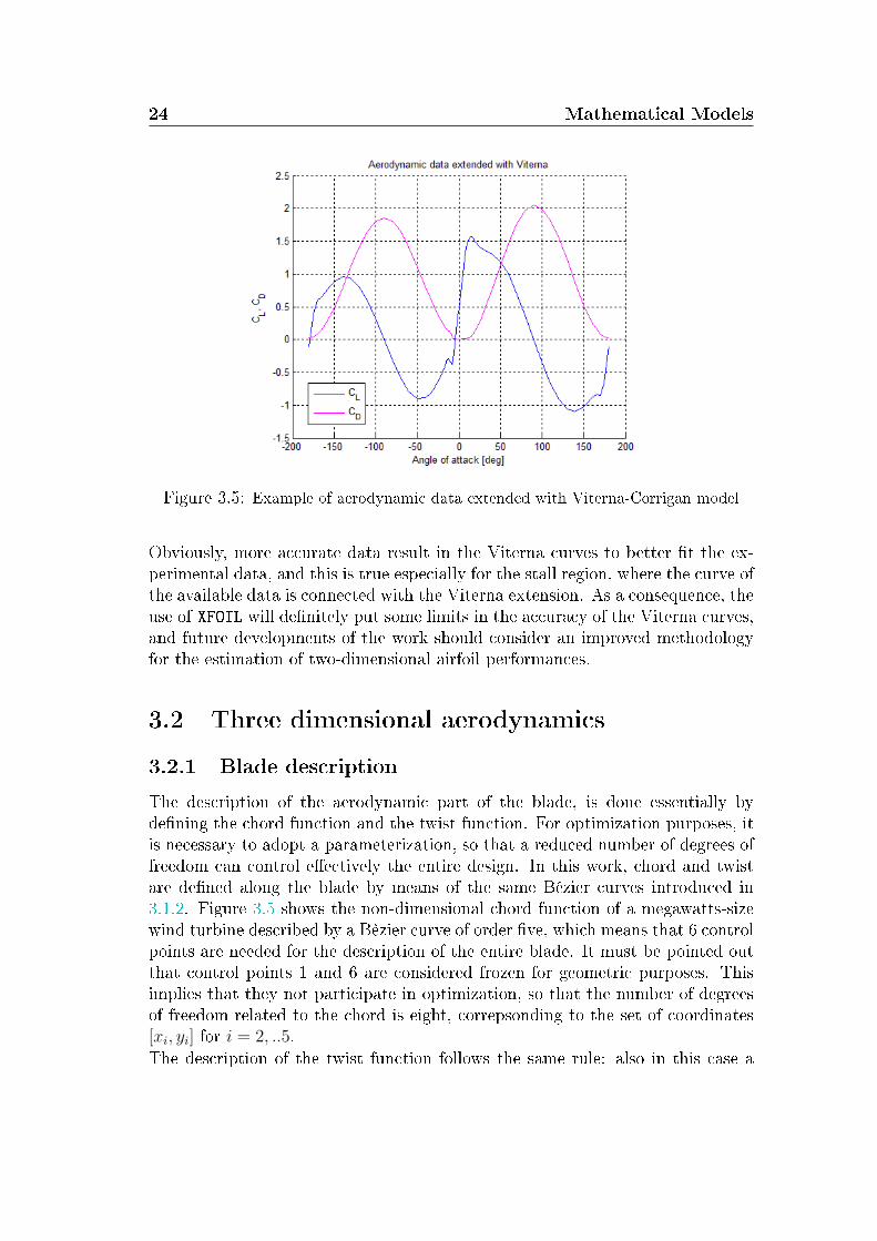
As it is evident, XFOIL fails to describe the near-stall and the post-stall regionsand, generally, it computes a signicant higher lift. The dual situation happensfor the negative stall, where a lower lift is computed. This peculiar beahviourmust be handled with care, as it puts a serious limit on the usage of XFOIL, andpanel methods in general, for the evaluation of wind turbines airfoils. In fact,usually a full characterization of the stall region is required in order to gain a fulloverview of the aero-elastic behaviour of the blade, as stall-induced vibrationscould trigger utter mechanisms [18]. In this work, where aeroelasticity is notaccounted for and where the aerodynamics is considered steady, this is not arelevant problem. Vice versa, a more striking consideration concerns the Viternamodel, which basically makes use of the at plate theory in order to extend theairfoil data from the region after stall to the entire range of angles of attack. Anexample of the typical resulting curves for the lift and the drag coecients isshown in Figure 3.5.
24 Mathematical Models
Figure 3.5: Example of aerodynamic data extended with Viterna-Corrigan model
Obviously, more accurate data result in the Viterna curves to better t the ex-perimental data, and this is true especially for the stall region, where the curve ofthe available data is connected with the Viterna extension. As a consequence, theuse of XFOIL will denitely put some limits in the accuracy of the Viterna curves,and future developments of the work should consider an improved methodologyfor the estimation of two-dimensional airfoil performances.
3.2 Three dimensional aerodynamics
3.2.1 Blade description
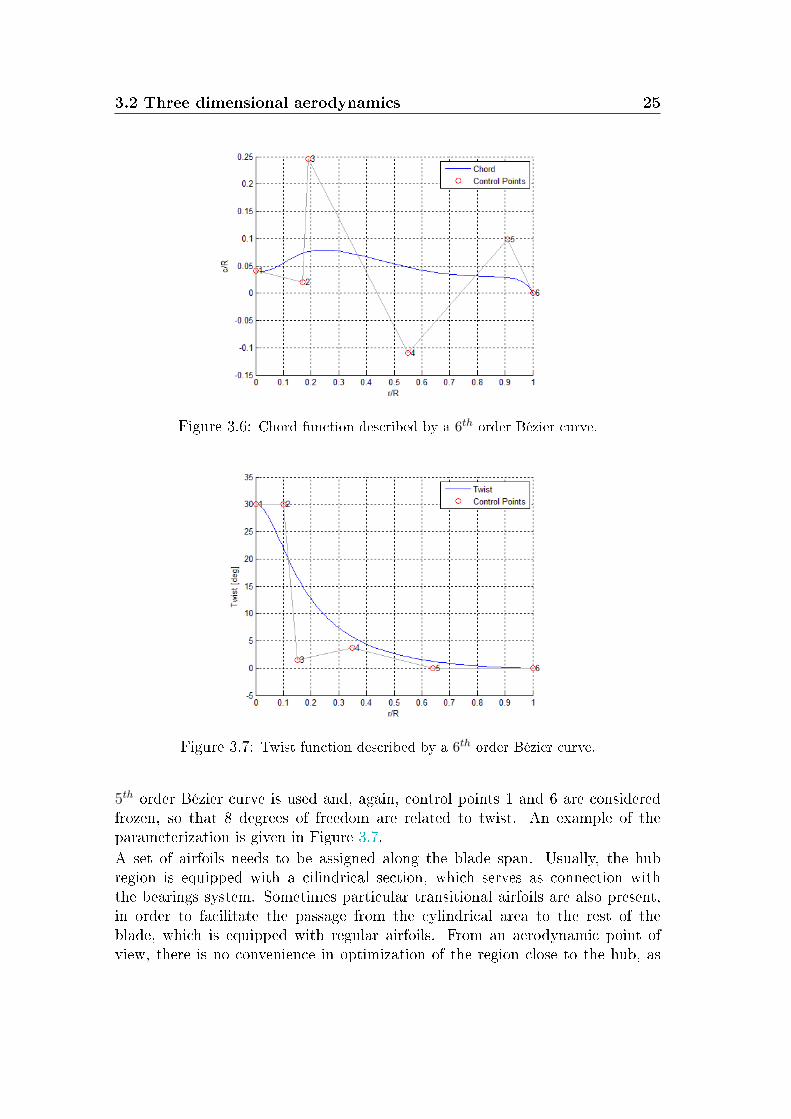
The description of the aerodynamic part of the blade, is done essentially bydening the chord function and the twist function. For optimization purposes, itis necessary to adopt a parameterization, so that a reduced number of degrees offreedom can control eectively the entire design. In this work, chord and twistare dened along the blade by means of the same Bézier curves introduced in3.1.2. Figure 3.5 shows the non-dimensional chord function of a megawatts-sizewind turbine described by a Bèzier curve of order ve, which means that 6 controlpoints are needed for the description of the entire blade. It must be pointed outthat control points 1 and 6 are considered frozen for geometric purposes. Thisimplies that they not participate in optimization, so that the number of degreesof freedom related to the chord is eight, correpsonding to the set of coordinates[xi, yi] for i = 2, ..5.The description of the twist function follows the same rule: also in this case a
3.2 Three dimensional aerodynamics 25
Figure 3.6: Chord function described by a 6th order Bézier curve.
Figure 3.7: Twist function described by a 6th order Bézier curve.
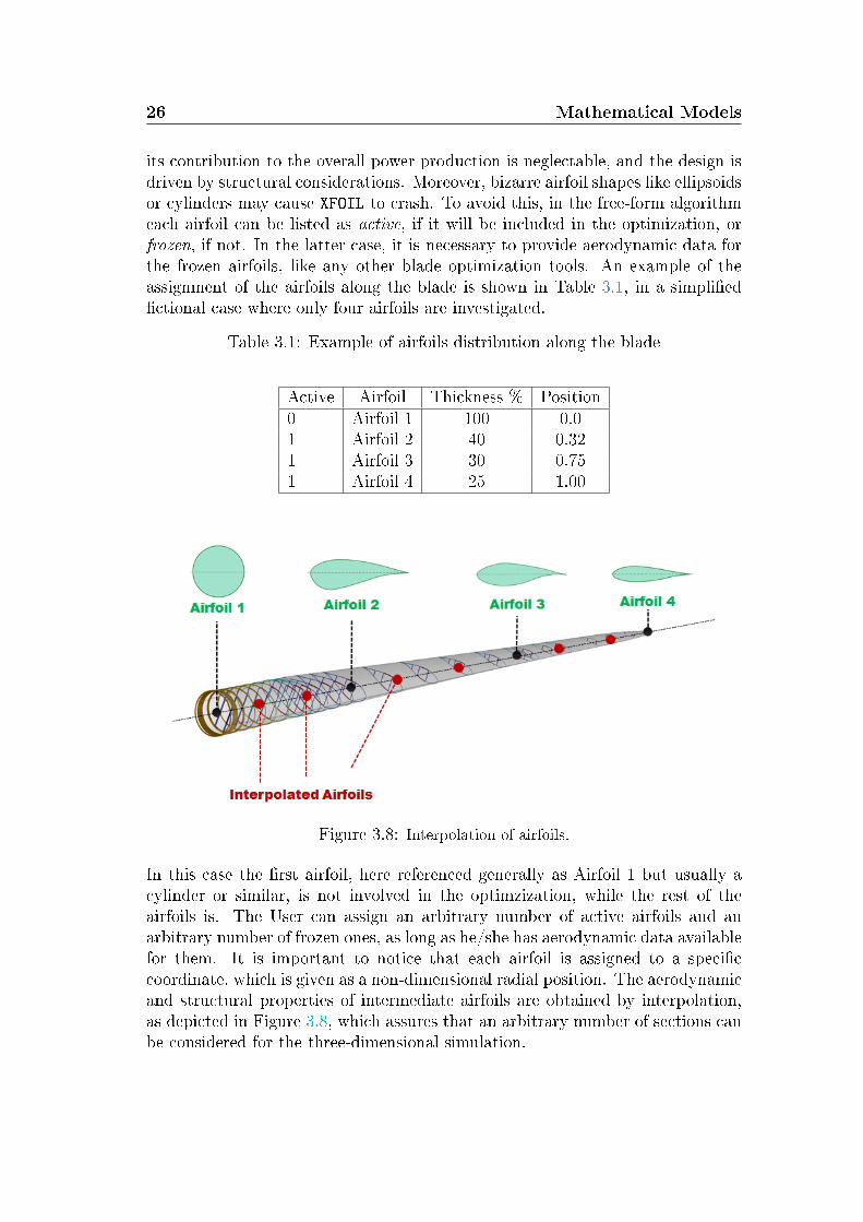
5th order Bézier curve is used and, again, control points 1 and 6 are consideredfrozen, so that 8 degrees of freedom are related to twist. An example of theparameterization is given in Figure 3.7.
A set of airfoils needs to be assigned along the blade span. Usually, the hubregion is equipped with a cilindrical section, which serves as connection withthe bearings system. Sometimes particular transitional airfoils are also present,in order to facilitate the passage from the cylindrical area to the rest of theblade, which is equipped with regular airfoils. From an aerodynamic point ofview, there is no convenience in optimization of the region close to the hub, as
26 Mathematical Models
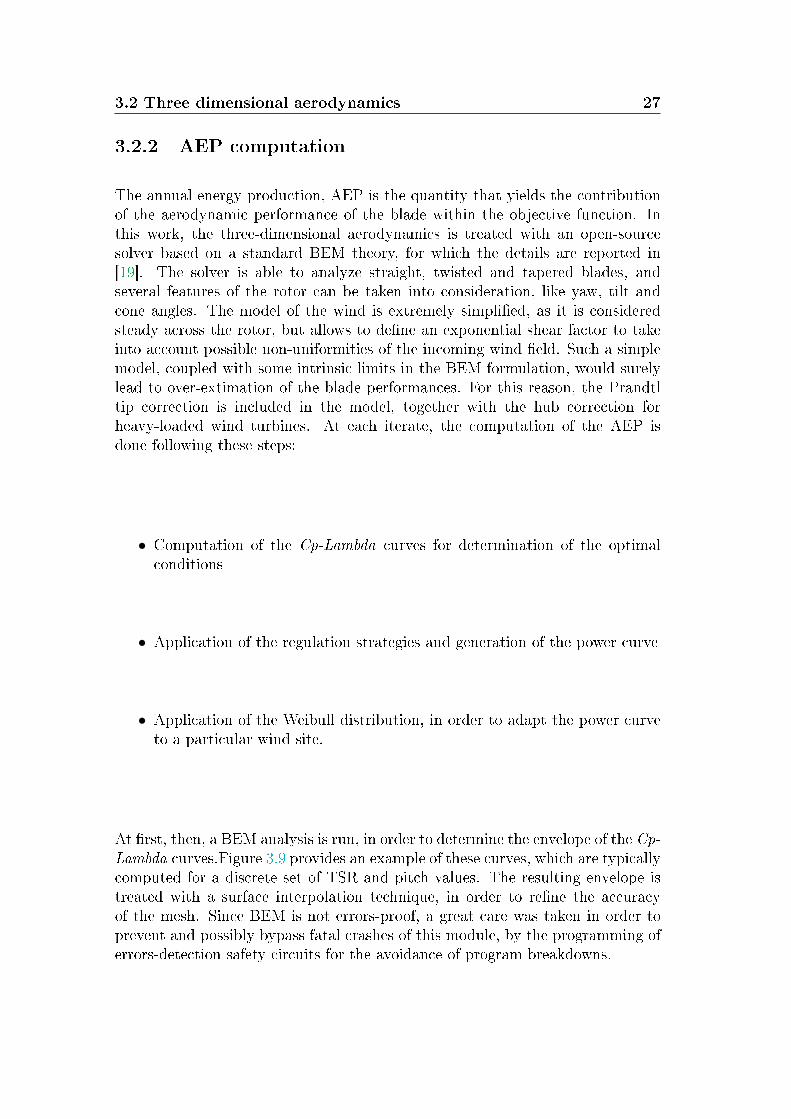
its contribution to the overall power production is neglectable, and the design isdriven by structural considerations. Moreover, bizarre airfoil shapes like ellipsoidsor cylinders may cause XFOIL to crash. To avoid this, in the free-form algorithmeach airfoil can be listed as active, if it will be included in the optimization, orfrozen, if not. In the latter case, it is necessary to provide aerodynamic data forthe frozen airfoils, like any other blade optimization tools. An example of theassignment of the airfoils along the blade is shown in Table 3.1, in a simpliedctional case where only four airfoils are investigated.
Table 3.1: Example of airfoils distribution along the blade
Active Airfoil Thickness % Position0 Airfoil 1 100 0.01 Airfoil 2 40 0.321 Airfoil 3 30 0.751 Airfoil 4 25 1.00
Figure 3.8: Interpolation of airfoils.
In this case the rst airfoil, here referenced generally as Airfoil 1 but usually acylinder or similar, is not involved in the optimzization, while the rest of theairfoils is. The User can assign an arbitrary number of active airfoils and anarbitrary number of frozen ones, as long as he/she has aerodynamic data availablefor them. It is important to notice that each airfoil is assigned to a speciccoordinate, which is given as a non-dimensional radial position. The aerodynamicand structural properties of intermediate airfoils are obtained by interpolation,as depicted in Figure 3.8, which assures that an arbitrary number of sections canbe considered for the three-dimensional simulation.
3.2 Three dimensional aerodynamics 27
3.2.2 AEP computation
The annual energy production, AEP is the quantity that yields the contributionof the aerodynamic performance of the blade within the objective function. Inthis work, the three-dimensional aerodynamics is treated with an open-sourcesolver based on a standard BEM theory, for which the details are reported in[19]. The solver is able to analyze straight, twisted and tapered blades, andseveral features of the rotor can be taken into consideration, like yaw, tilt andcone angles. The model of the wind is extremely simplied, as it is consideredsteady across the rotor, but allows to dene an exponential shear factor to takeinto account possible non-uniformities of the incoming wind eld. Such a simplemodel, coupled with some intrinsic limits in the BEM formulation, would surelylead to over-extimation of the blade performances. For this reason, the Prandtltip correction is included in the model, together with the hub correction forheavy-loaded wind turbines. At each iterate, the computation of the AEP isdone following these steps:
• Computation of the Cp-Lambda curves for determination of the optimalconditions
• Application of the regulation strategies and generation of the power curve
• Application of the Weibull distribution, in order to adapt the power curveto a particular wind site.
At rst, then, a BEM analysis is run, in order to determine the envelope of the Cp-Lambda curves.Figure 3.9 provides an example of these curves, which are typicallycomputed for a discrete set of TSR and pitch values. The resulting envelope istreated with a surface interpolation technique, in order to rene the accuracyof the mesh. Since BEM is not errors-proof, a great care was taken in order toprevent and possibly bypass fatal crashes of this module, by the programming oferrors-detection safety circuits for the avoidance of program breakdowns.
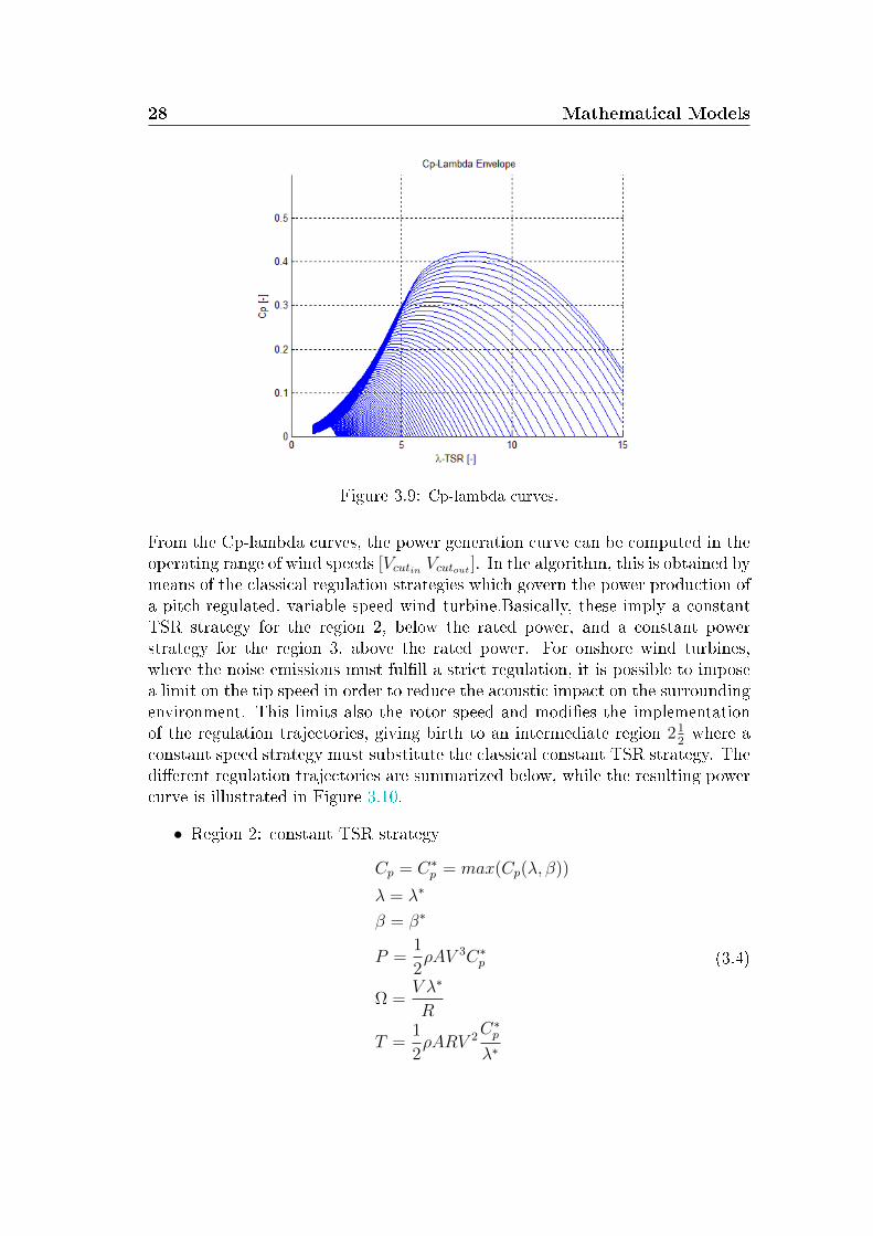
28 Mathematical Models
Figure 3.9: Cp-lambda curves.
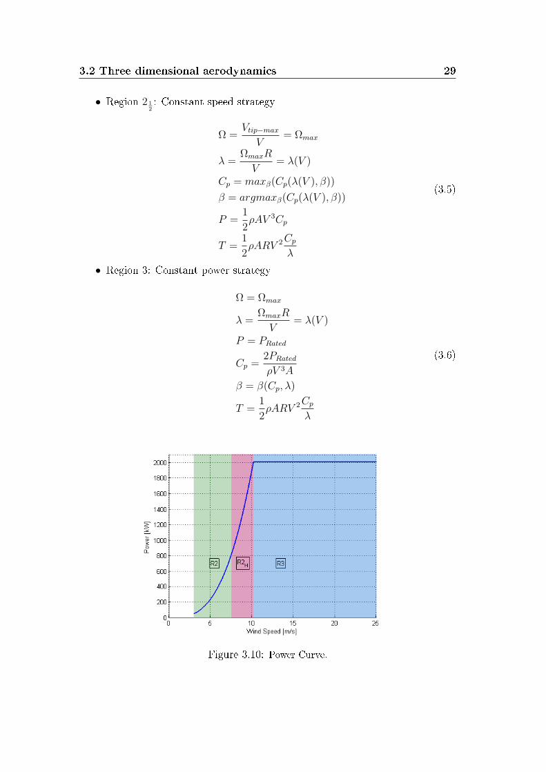
From the Cp-lambda curves, the power generation curve can be computed in theoperating range of wind speeds [Vcutin Vcutout ]. In the algorithm, this is obtained bymeans of the classical regulation strategies which govern the power production ofa pitch-regulated, variable speed wind turbine.Basically, these imply a constantTSR strategy for the region 2, below the rated power, and a constant powerstrategy for the region 3, above the rated power. For onshore wind turbines,where the noise emissions must fulll a strict regulation, it is possible to imposea limit on the tip speed in order to reduce the acoustic impact on the surroundingenvironment. This limits also the rotor speed and modies the implementationof the regulation trajectories, giving birth to an intermediate region 21
2where a
constant speed strategy must substitute the classical constant TSR strategy. Thedierent regulation trajectories are summarized below, while the resulting powercurve is illustrated in Figure 3.10.
• Region 2: constant TSR strategy
Cp = C∗p = max(Cp(λ, β))
λ = λ∗
β = β∗
P =1
2ρAV 3C∗
p
Ω =V λ∗
R
T =1
2ρARV 2
C∗p
λ∗
(3.4)
3.2 Three dimensional aerodynamics 29
• Region 2 12: Constant speed strategy
Ω =Vtip−max
V= Ωmax
λ =ΩmaxR
V= λ(V )
Cp = maxβ(Cp(λ(V ), β))
β = argmaxβ(Cp(λ(V ), β))
P =1
2ρAV 3Cp
T =1
2ρARV 2Cp
λ
(3.5)
• Region 3: Constant power strategy
Ω = Ωmax
λ =ΩmaxR
V= λ(V )
P = PRated
Cp =2PRated
ρV 3A
β = β(Cp, λ)
T =1
2ρARV 2Cp
λ
(3.6)
Figure 3.10: Power Curve.
30 Mathematical Models
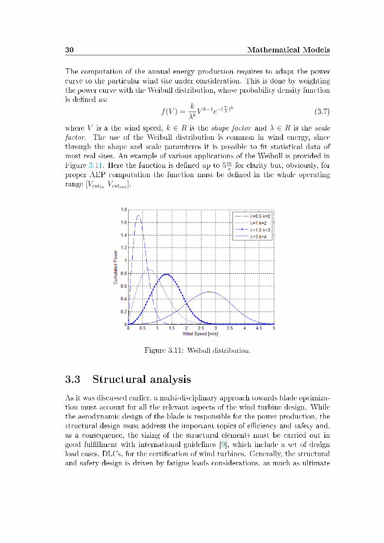
The computation of the annual energy production requires to adapt the powercurve to the particular wind site under consideration. This is done by weightingthe power curve with the Weibull distribution, whose probability density functionis dened as:
f(V ) =k
λkV k−1e−(V
λ)k (3.7)
where V is a the wind speed, k ∈ R is the shape factor and λ ∈ R is the scalefactor. The use of the Weibull distribution is common in wind energy, sincethrough the shape and scale paramteres it is possible to t statistical data ofmost real sites. An example of various applications of the Weibull is provided inFigure 3.11. Here the function is dened up to 5m
sfor clarity but, obviously, for
proper AEP computation the function must be dened in the whole operatingrange [Vcutin Vcutout ].
Figure 3.11: Weibull distribution.
3.3 Structural analysis
As it was discussed earlier, a multi-disciplinary approach towards blade optimiza-tion must account for all the relevant aspects of the wind turbine design. Whilethe aerodynamic design of the blade is responsible for the power production, thestructural design must address the important topics of eciency and safety and,as a consequence, the sizing of the structural elements must be carried out ingood fulllment with international guidelines [9], which include a set of designload cases, DLCs, for the certication of wind turbines. Generally, the structuraland safety design is driven by fatigue loads considerations, as much as ultimate
3.3 Structural analysis 31
loads analysis and instability avoidance, when complex aero-elastic models areavailable. In this work our intention is to favour simplicity: the main scope is notdo develop a commercial code but rather to explore the implications of the free-form methodology and, for this reason, we chose to employ simplied versionsof DLCs, which result in the two constraints illustrated in section 2.2. In thefollowing, the models which constitute the structural simulations are discussed.
3.3.1 Description of the blade section
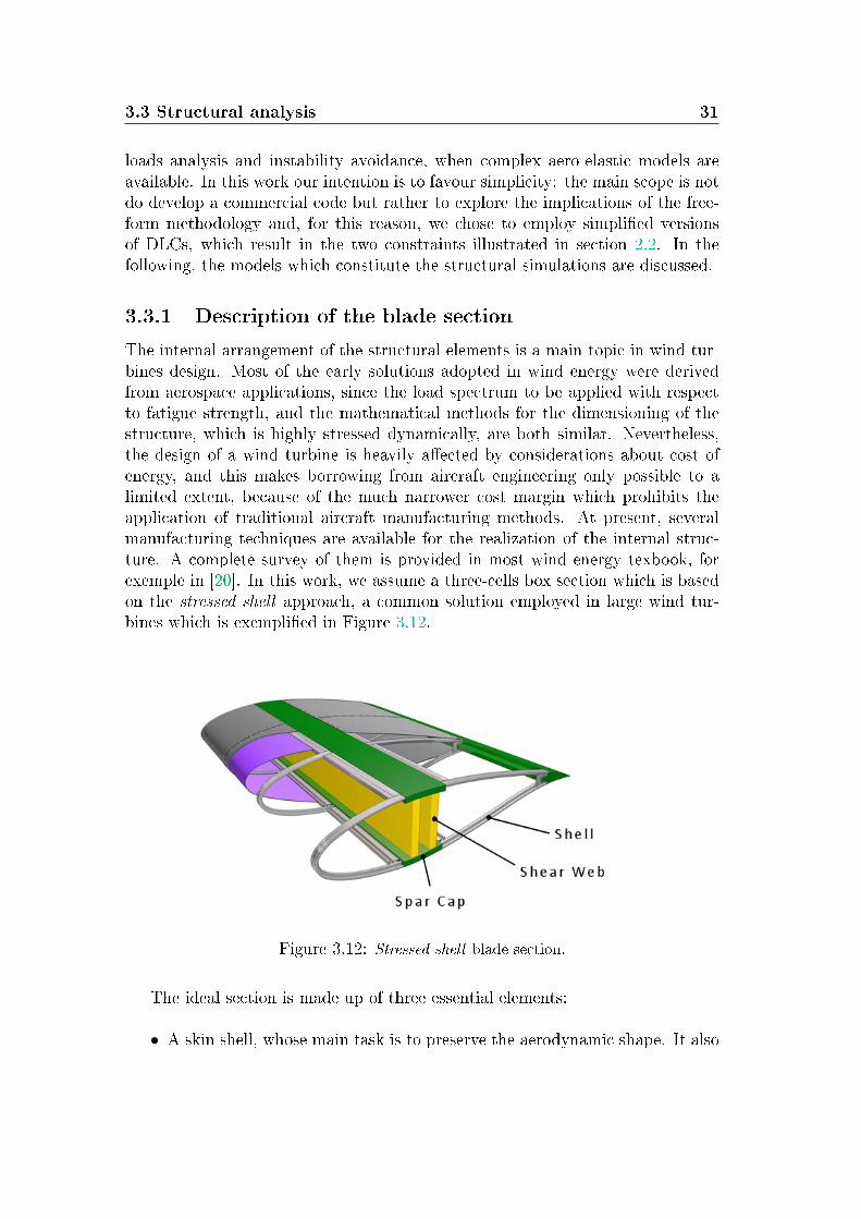
The internal arrangement of the structural elements is a main topic in wind tur-bines design. Most of the early solutions adopted in wind energy were derivedfrom aerospace applications, since the load spectrum to be applied with respectto fatigue strength, and the mathematical methods for the dimensioning of thestructure, which is highly stressed dynamically, are both similar. Nevertheless,the design of a wind turbine is heavily aected by considerations about cost ofenergy, and this makes borrowing from aircraft engineering only possible to alimited extent, because of the much narrower cost margin which prohibits theapplication of traditional aircraft manufacturing methods. At present, severalmanufacturing techniques are available for the realization of the internal struc-ture. A complete survey of them is provided in most wind energy texbook, forexemple in [20]. In this work, we assume a three-cells box section which is basedon the stressed shell approach, a common solution employed in large wind tur-bines which is exemplied in Figure 3.12.
Figure 3.12: Stressed shell blade section.
The ideal section is made up of three essential elements:
• A skin shell, whose main task is to preserve the aerodynamic shape. It also
32 Mathematical Models
plays a structural role in stiening and strengthening the spar, particularlyto resist torsion (twisting) loads.
• Two spar caps, which bear the signicative bending moment acting alongthe blade.
• Two shear webs which are connected to the other elements in order to grantthe required shear strength.
This formulation is quite essential and it simplies the actual techniques of bladeconstruction. Thus, some aspects of the manifacture are neglected like, for ex-ample, the fact that usually the shear webs are made up of composite layers lledwith foam or a core material, in order to prevent buckling phenomena due to ahigh compressive stress. Modern blade sections are also equipped with leadingedge and trailing edge reinforcements in order to increase the in-plane stiness.However, it must be noticed that the constraints employed in this work concernmainly the out-of plane deections and the stress in the spar cap, for which thesimplied structure adopted is perfectly adequate. It should be easy, in futuredevelopments, to introduce a more accurate description of the blade section, inorder to account for buckling verication or torsional stress evaluation, if needed.
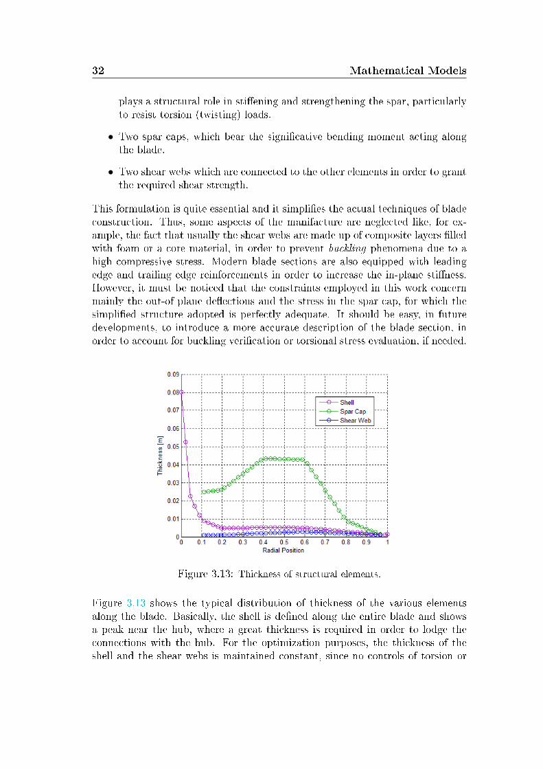
Figure 3.13: Thickness of structural elements.
Figure 3.13 shows the typical distribution of thickness of the various elementsalong the blade. Basically, the shell is dened along the entire blade and showsa peak near the hub, where a great thickness is required in order to lodge theconnections with the hub. For the optimization purposes, the thickness of theshell and the shear webs is maintained constant, since no controls of torsion or
3.3 Structural analysis 33
buckling are currently present in the program, and leaving them free to changecould lead to an overestimation of the structural performances. On the contrary,the spar cap thickness is left free to optimization, and the User can specify anarbitrary number of degrees of freedom related to the spar cap thickness in orderto tune the sensitivity of the optimization to his/her goals.
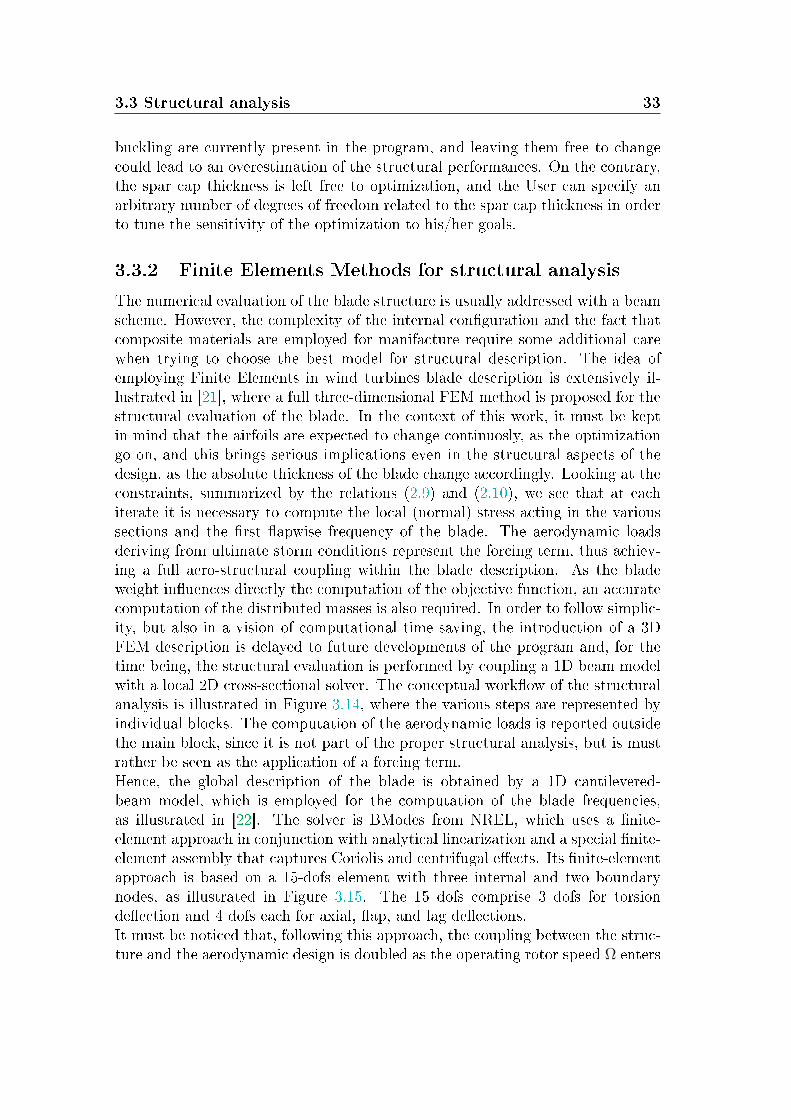
3.3.2 Finite Elements Methods for structural analysis
The numerical evaluation of the blade structure is usually addressed with a beamscheme. However, the complexity of the internal conguration and the fact thatcomposite materials are employed for manifacture require some additional carewhen trying to choose the best model for structural description. The idea ofemploying Finite Elements in wind turbines blade description is extensively il-lustrated in [21], where a full three-dimensional FEM method is proposed for thestructural evaluation of the blade. In the context of this work, it must be keptin mind that the airfoils are expected to change continuosly, as the optimizationgo on, and this brings serious implications even in the structural aspects of thedesign, as the absolute thickness of the blade change accordingly. Looking at theconstraints, summarized by the relations (2.9) and (2.10), we see that at eachiterate it is necessary to compute the local (normal) stress acting in the varioussections and the rst apwise frequency of the blade. The aerodynamic loadsderiving from ultimate storm conditions represent the forcing term, thus achiev-ing a full aero-structural coupling within the blade description. As the bladeweight inuences directly the computation of the objective function, an accuratecomputation of the distributed masses is also required. In order to follow simplic-ity, but also in a vision of computational time saving, the introduction of a 3DFEM description is delayed to future developments of the program and, for thetime being, the structural evaluation is performed by coupling a 1D beam modelwith a local 2D cross-sectional solver. The conceptual workow of the structuralanalysis is illustrated in Figure 3.14, where the various steps are represented byindividual blocks. The computation of the aerodynamic loads is reported outsidethe main block, since it is not part of the proper structural analysis, but is mustrather be seen as the application of a forcing term.Hence, the global description of the blade is obtained by a 1D cantilevered-beam model, which is employed for the computation of the blade frequencies,as illustrated in [22]. The solver is BModes from NREL, which uses a nite-element approach in conjunction with analytical linearization and a special nite-element assembly that captures Coriolis and centrifugal eects. Its nite-elementapproach is based on a 15-dofs element with three internal and two boundarynodes, as illustrated in Figure 3.15. The 15 dofs comprise 3 dofs for torsiondeection and 4 dofs each for axial, ap, and lag deections.It must be noticed that, following this approach, the coupling between the struc-ture and the aerodynamic design is doubled as the operating rotor speed Ω enters
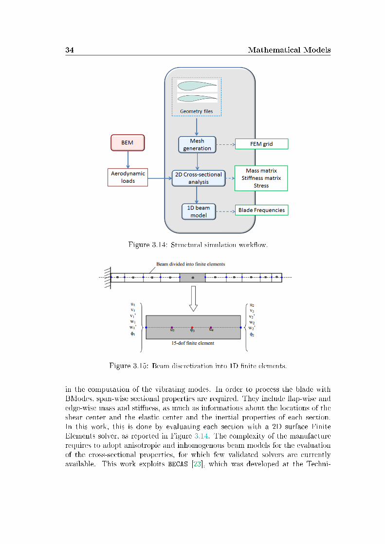
34 Mathematical Models
Figure 3.14: Structural simulation workow.
Figure 3.15: Beam discretization into 1D nite elements.
in the computation of the vibrating modes. In order to process the blade withBModes, span-wise sectional properties are required. They include ap-wise andedge-wise mass and stiness, as much as informations about the locations of theshear center and the elastic center and the inertial properties of each section.In this work, this is done by evaluating each section with a 2D surface FiniteElements solver, as reported in Figure 3.14. The complexity of the manufacturerequires to adopt anisotropic and inhomogenous beam models for the evaluationof the cross-sectional properties, for which few validated solvers are currentlyavailable. This work exploits BECAS [23], which was developed at the Techni-
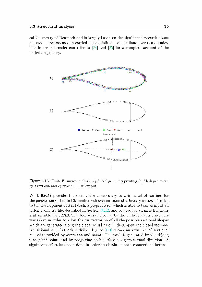
3.3 Structural analysis 35
cal University of Denmark and is largely based on the signicant research aboutanisotropic beams models carried out at Politecnico di Milano over two decades.The interested reader can refer to [24] and [25] for a complete account of theunderlying theory.
Figure 3.16: Finite Elements analysis. a) Airfoil geometry pivoting, b) Mesh generated
by AirfMesh and c) typical BECAS output.
While BECAS provides the solver, it was necessary to write a set of routines forthe generation of Finite Elements mesh over sections of arbitrary shape. This ledto the development of AirfMesh, a preprocessor which is able to take as input anairfoil geometry le, described in Section 3.1.2, and to produce a Finite Elementsgrid suitable for BECAS. The tool was developed by the author, and a great carewas taken in order to allow the discretization of all the possible sectional shapeswhich are generated along the blade including cylinders, open and closed sections,transitional and atback airfoils. Figure 3.16 shows an example of sectionalanalysis provided by AirfMesh and BECAS. The mesh is generated by identifyingnine pivot points and by projecting each surface along its normal direction. Asignicant eort has been done in order to obtain smooth connections between
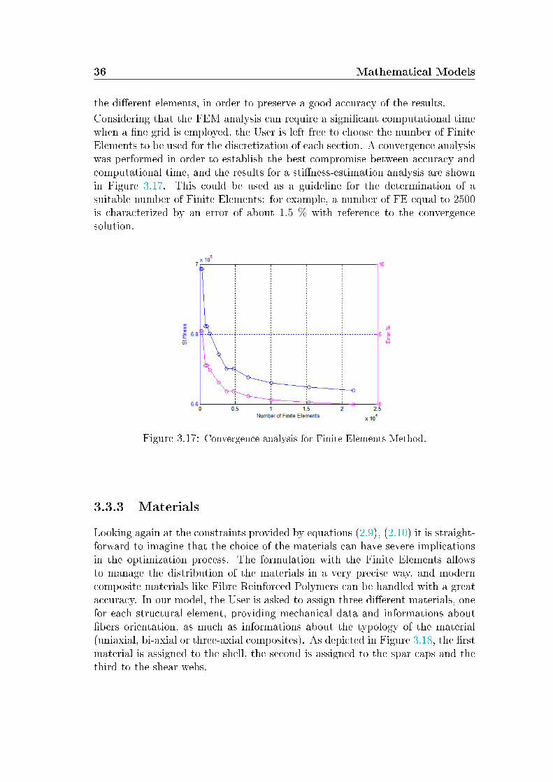
36 Mathematical Models
the dierent elements, in order to preserve a good accuracy of the results.
Considering that the FEM analysis can require a signicant computational timewhen a ne grid is employed, the User is left free to choose the number of FiniteElements to be used for the discretization of each section. A convergence analysiswas performed in order to establish the best compromise between accuracy andcomputational time, and the results for a stiness-estimation analysis are shownin Figure 3.17. This could be used as a guideline for the determination of asuitable number of Finite Elements: for example, a number of FE equal to 2500is characterized by an error of about 1.5 % with reference to the convergencesolution.
Figure 3.17: Convergence analysis for Finite Elements Method.
3.3.3 Materials
Looking again at the constraints provided by equations (2.9), (2.10) it is straight-forward to imagine that the choice of the materials can have severe implicationsin the optimization process. The formulation with the Finite Elements allowsto manage the distribution of the materials in a very precise way, and moderncomposite materials like Fibre Reinforced Polymers can be handled with a greataccuracy. In our model, the User is asked to assign three dierent materials, onefor each structural element, providing mechanical data and informations aboutbers orientation, as much as informations about the typology of the material(uniaxial, bi-axial or three-axial composites). As depicted in Figure 3.18, the rstmaterial is assigned to the shell, the second is assigned to the spar caps and thethird to the shear webs,
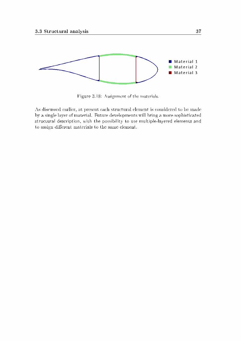
3.3 Structural analysis 37
Figure 3.18: Assignment of the materials.
As discussed earlier, at present each structural element is considered to be madeby a single layer of material. Future developments will bring a more sophisticatedstructural description, with the possibility to use multiple-layered elements andto assign dierent materials to the same element.


Chapter 4
Case Studies
In this Chapter, we provide examples of the application of the free-form method-ology. The algorithm developed in this work is employed for the optimization ofrotor blades taken from real-world machines. The main goals are to validate theprogram, to assure that it can represent a baseline wind turbine with a satisfac-tory level of accuracy, and to verify the behaviour of the free-form methodology,in order to understand if it can oer improvements to the traditional optimizationstrategies.
4.1 Reference 2 MW wind turbine
The rst case study concerns a typical megawatt-size wind turbine which, forbrevity, will be hereafter referenced as the REF45-2.0 wind turbine. The designwas carried out by ECN and Politecnico di Milano, and the features are typicalof a modern variable speed, pitch-regulated wind turbine designed for strength.The main features of the wind turbine are listed in Table 4.1.
Class IEC IIIARotor orientation Clockwise, upwind
Control Variable speed, collective pitchCut in speed 3 m/sCut out speed 25 m/sRated power 2.0 MW
Number of blades 3Rotor radius 46.2 mHub Radius 1.2 mCone angle 1.0 deg
Table 4.1: REF45-2.0 wind turbine: overall characteristics
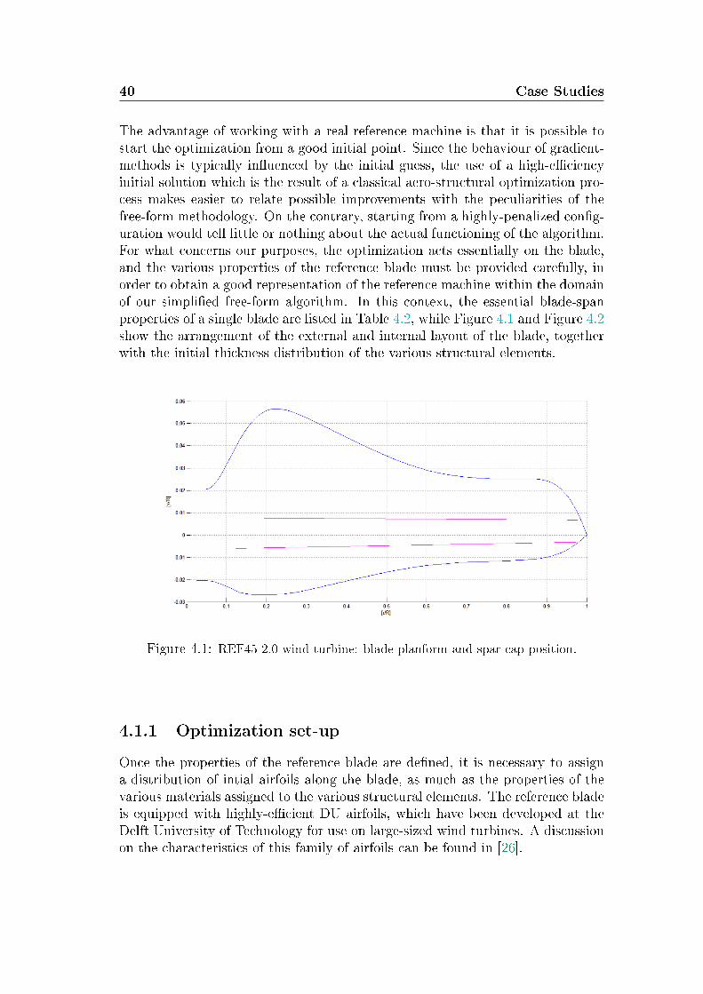
40 Case Studies
The advantage of working with a real reference machine is that it is possible tostart the optimization from a good initial point. Since the behaviour of gradient-methods is typically inuenced by the initial guess, the use of a high-eciencyinitial solution which is the result of a classical aero-structural optimization pro-cess makes easier to relate possible improvements with the peculiarities of thefree-form methodology. On the contrary, starting from a highly-penalized cong-uration would tell little or nothing about the actual functioning of the algorithm.For what concerns our purposes, the optimization acts essentially on the blade,and the various properties of the reference blade must be provided carefully, inorder to obtain a good representation of the reference machine within the domainof our simplied free-form algorithm. In this context, the essential blade-spanproperties of a single blade are listed in Table 4.2, while Figure 4.1 and Figure 4.2show the arrangement of the external and internal layout of the blade, togetherwith the initial thickness distribution of the various structural elements.
Figure 4.1: REF45-2.0 wind turbine: blade planform and spar cap position.
4.1.1 Optimization set-up
Once the properties of the reference blade are dened, it is necessary to assigna distribution of intial airfoils along the blade, as much as the properties of thevarious materials assigned to the various structural elements. The reference bladeis equipped with highly-ecient DU airfoils, which have been developed at theDelft University of Technology for use on large-sized wind turbines. A discussionon the characteristics of this family of airfoils can be found in [26].
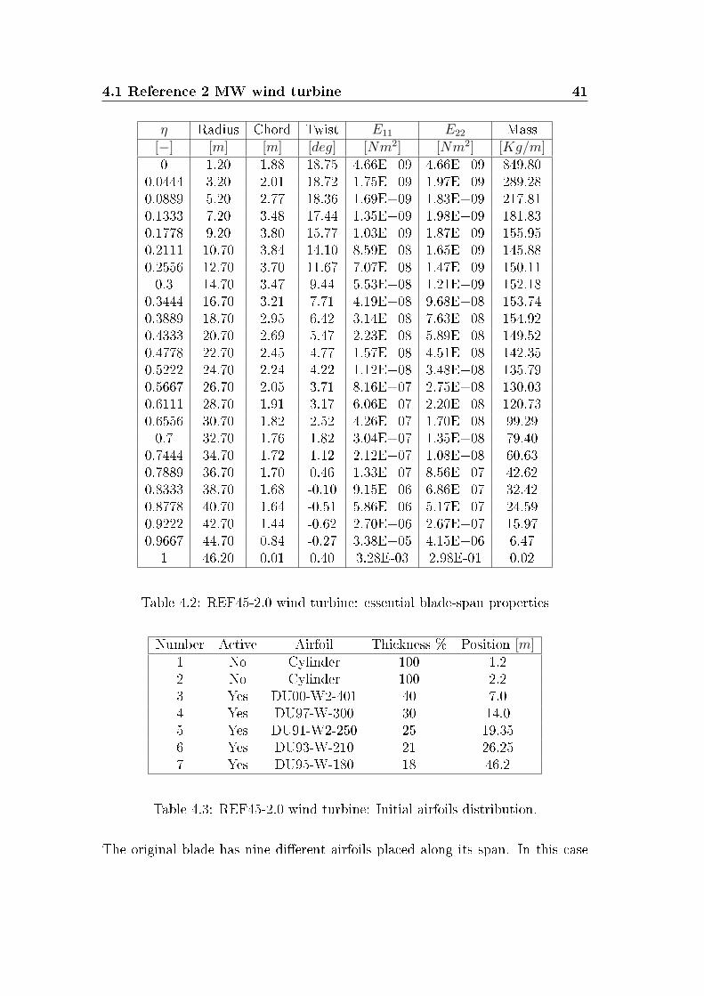
4.1 Reference 2 MW wind turbine 41
η Radius Chord Twist E11 E22 Mass[−] [m] [m] [deg] [Nm2] [Nm2] [Kg/m]0 1.20 1.88 18.75 4.66E+09 4.66E+09 849.80
0.0444 3.20 2.01 18.72 1.75E+09 1.97E+09 289.280.0889 5.20 2.77 18.36 1.69E+09 1.83E+09 217.810.1333 7.20 3.48 17.44 1.35E+09 1.98E+09 181.830.1778 9.20 3.80 15.77 1.03E+09 1.87E+09 155.950.2111 10.70 3.84 14.10 8.59E+08 1.65E+09 145.880.2556 12.70 3.70 11.67 7.07E+08 1.47E+09 150.110.3 14.70 3.47 9.44 5.53E+08 1.21E+09 152.18
0.3444 16.70 3.21 7.71 4.19E+08 9.68E+08 153.740.3889 18.70 2.95 6.42 3.14E+08 7.63E+08 154.920.4333 20.70 2.69 5.47 2.23E+08 5.89E+08 149.520.4778 22.70 2.45 4.77 1.57E+08 4.51E+08 142.350.5222 24.70 2.24 4.22 1.12E+08 3.48E+08 135.790.5667 26.70 2.05 3.71 8.16E+07 2.75E+08 130.030.6111 28.70 1.91 3.17 6.06E+07 2.20E+08 120.730.6556 30.70 1.82 2.52 4.26E+07 1.70E+08 99.290.7 32.70 1.76 1.82 3.04E+07 1.35E+08 79.40
0.7444 34.70 1.72 1.12 2.12E+07 1.08E+08 60.630.7889 36.70 1.70 0.46 1.33E+07 8.56E+07 42.620.8333 38.70 1.68 -0.10 9.15E+06 6.86E+07 32.420.8778 40.70 1.64 -0.51 5.86E+06 5.17E+07 24.590.9222 42.70 1.44 -0.62 2.70E+06 2.67E+07 15.970.9667 44.70 0.84 -0.27 3.38E+05 4.15E+06 6.47
1 46.20 0.01 0.40 3.28E-03 2.98E-01 0.02
Table 4.2: REF45-2.0 wind turbine: essential blade-span properties
Number Active Airfoil Thickness % Position [m]1 No Cylinder 100 1.22 No Cylinder 100 2.23 Yes DU00-W2-401 40 7.04 Yes DU97-W-300 30 14.05 Yes DU91-W2-250 25 19.356 Yes DU93-W-210 21 26.257 Yes DU95-W-180 18 46.2
Table 4.3: REF45-2.0 wind turbine: Initial airfoils distribution.
The original blade has nine dierent airfoils placed along its span. In this case
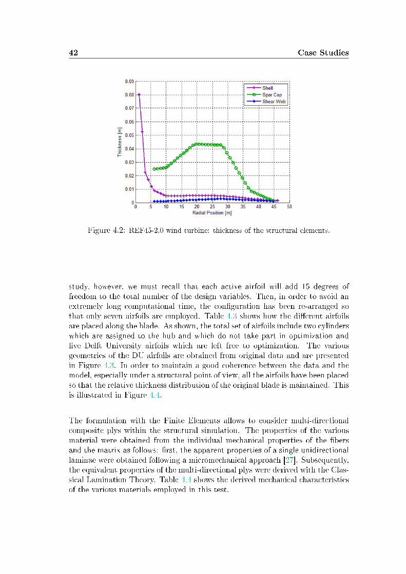
42 Case Studies
Figure 4.2: REF45-2.0 wind turbine: thickness of the structural elements.
study, however, we must recall that each active airfoil will add 15 degrees offreedom to the total number of the design variables. Then, in order to avoid anextremely long computational time, the conguration has been re-arranged sothat only seven airfoils are employed. Table 4.3 shows how the dierent airfoilsare placed along the blade. As shown, the total set of airfoils include two cylinderswhich are assigned to the hub and which do not take part in optimization andve Delft University airfoils which are left free to optimization. The variousgeometries of the DU airfoils are obtained from original data and are presentedin Figure 4.3. In order to maintain a good coherence between the data and themodel, especially under a structural point of view, all the airfoils have been placedso that the relative thickness distribution of the original blade is maintained. Thisis illustrated in Figure 4.4.
The formulation with the Finite Elements allows to consider multi-directionalcomposite plys within the structural simulation. The properties of the variousmaterial were obtained from the individual mechanical properties of the bersand the matrix as follows: rst, the apparent properties of a single unidirectionallaminae were obtained following a micromechanical approach [27]. Subsequently,the equivalent properties of the multi-directional plys were derived with the Clas-sical Lamination Theory. Table 4.4 shows the derived mechanical characteristicsof the various materials employed in this test.
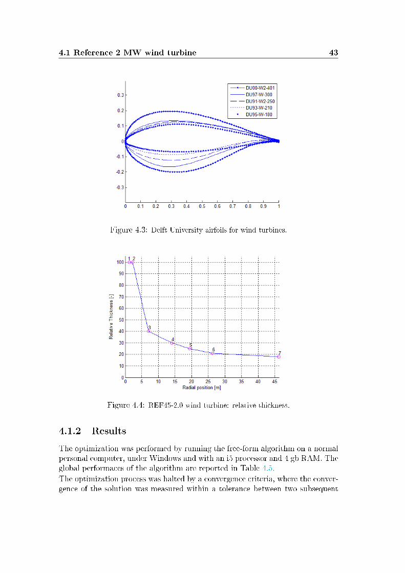
4.1 Reference 2 MW wind turbine 43
Figure 4.3: Delft University airfoils for wind turbines.
Figure 4.4: REF45-2.0 wind turbine: relative thickness.
4.1.2 Results
The optimization was performed by running the free-form algorithm on a normalpersonal computer, under Windows and with an i5 processor and 4 gb RAM. Theglobal performaces of the algorithm are reported in Table 4.5.
The optimization process was halted by a convergence criteria, where the conver-gence of the solution was measured within a tolerance between two subsequent
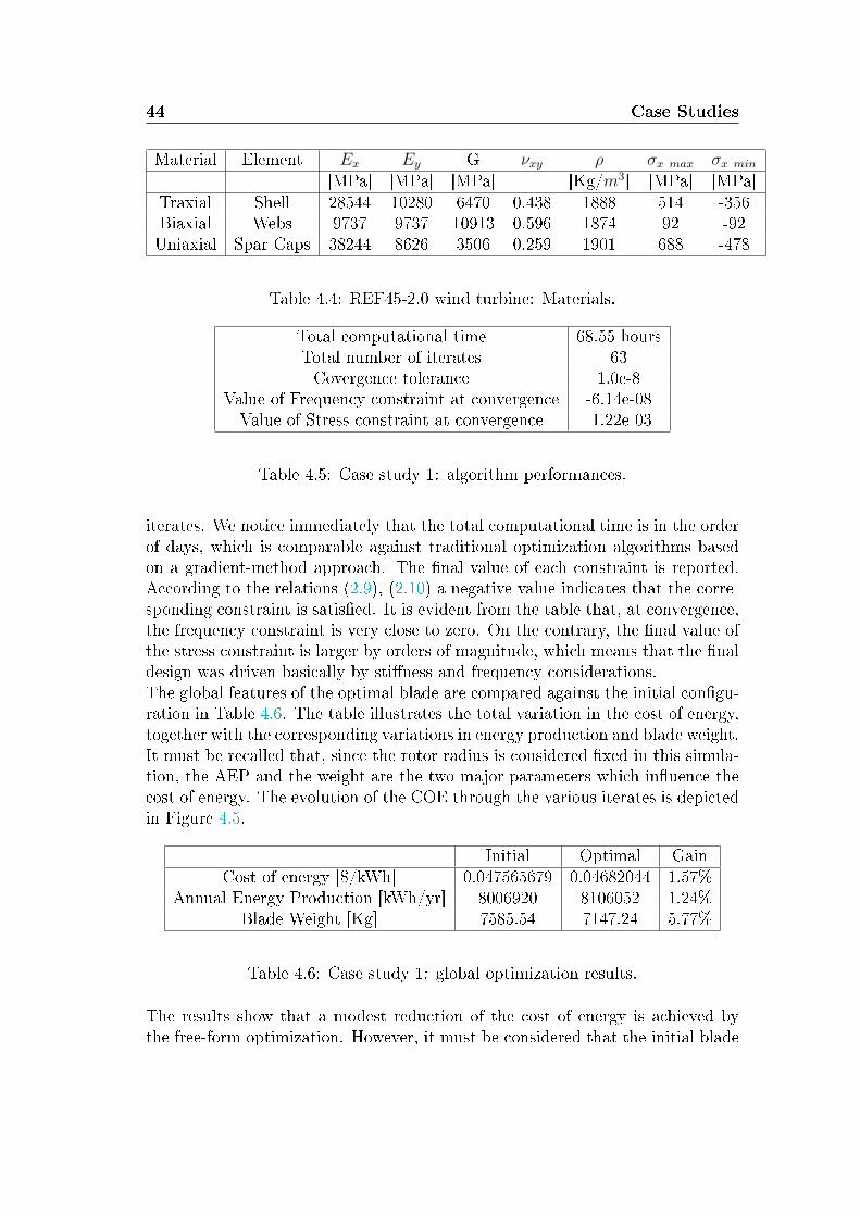
44 Case Studies
Material Element Ex Ey G νxy ρ σx max σx min
[MPa] [MPa] [MPa] [Kg/m3] [MPa] [MPa]Traxial Shell 28544 10280 6470 0.438 1888 514 -356Biaxial Webs 9737 9737 10913 0.596 1874 92 -92Uniaxial Spar Caps 38244 8626 3506 0.259 1901 688 -478
Table 4.4: REF45-2.0 wind turbine: Materials.
Total computational time 68.55 hoursTotal number of iterates 63Covergence tolerance 1.0e-8
Value of Frequency constraint at convergence -6.14e-08Value of Stress constraint at convergence -1.22e-03
Table 4.5: Case study 1: algorithm performances.
iterates. We notice immediately that the total computational time is in the orderof days, which is comparable against traditional optimization algorithms basedon a gradient-method approach. The nal value of each constraint is reported.According to the relations (2.9), (2.10) a negative value indicates that the corre-sponding constraint is satised. It is evident from the table that, at convergence,the frequency constraint is very close to zero. On the contrary, the nal value ofthe stress constraint is larger by orders of magnitude, which means that the naldesign was driven basically by stiness and frequency considerations.The global features of the optimal blade are compared against the initial congu-ration in Table 4.6. The table illustrates the total variation in the cost of energy,together with the corresponding variations in energy production and blade weight.It must be recalled that, since the rotor radius is considered xed in this simula-tion, the AEP and the weight are the two major parameters which inuence thecost of energy. The evolution of the COE through the various iterates is depictedin Figure 4.5.
Initial Optimal GainCost of energy [$/kWh] 0.047565679 0.04682044 1.57%
Annual Energy Production [kWh/yr] 8006920 8106052 1.24%Blade Weight [Kg] 7585.54 7147.24 5.77%
Table 4.6: Case study 1: global optimization results.
The results show that a modest reduction of the cost of energy is achieved bythe free-form optimization. However, it must be considered that the initial blade
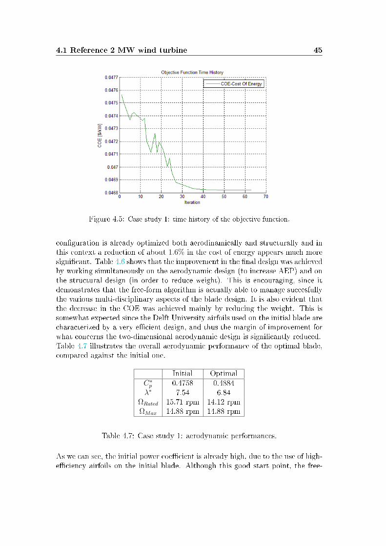
4.1 Reference 2 MW wind turbine 45
Figure 4.5: Case study 1: time history of the objective function.
conguration is already optimized both aerodinamically and structurally and inthis context a reduction of about 1.6% in the cost of energy appears much moresignicant. Table 4.6 shows that the improvement in the nal design was achievedby working simultaneously on the aerodynamic design (to increase AEP) and onthe structural design (in order to reduce weight). This is encouraging, since itdemonstrates that the free-form algorithm is actually able to manage succesfullythe various multi-disciplinary aspects of the blade design. It is also evident thatthe decrease in the COE was achieved mainly by reducing the weight. This issomewhat expected since the Delft University airfoils used on the initial blade arecharacterized by a very ecient design, and thus the margin of improvement forwhat concerns the two-dimensional aerodynamic design is signicantly reduced.Table 4.7 illustrates the overall aerodynamic performance of the optimal blade,compared against the initial one.
Initial OptimalC∗
p 0.4758 0.4884λ∗ 7.54 6.84
ΩRated 15.71 rpm 14.12 rpmΩMax 14.88 rpm 14.88 rpm
Table 4.7: Case study 1: aerodynamic performances.
As we can see, the initial power coecient is already high, due to the use of high-eciency airfoils on the initial blade. Although this good start point, the free-
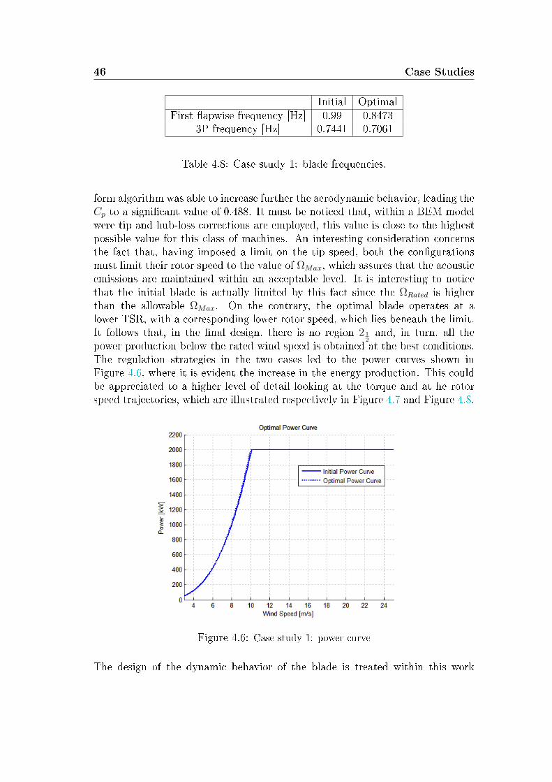
46 Case Studies
Initial OptimalFirst apwise frequency [Hz] 0.99 0.8473
3P frequency [Hz] 0.7441 0.7061
Table 4.8: Case study 1: blade frequencies.
form algorithm was able to increase further the aerodynamic behavior, leading theCp to a signicant value of 0.488. It must be noticed that, within a BEM modelwere tip and hub-loss corrections are employed, this value is close to the highestpossible value for this class of machines. An interesting consideration concernsthe fact that, having imposed a limit on the tip speed, both the congurationsmust limit their rotor speed to the value of ΩMax, which assures that the acousticemissions are maintained within an acceptable level. It is interesting to noticethat the initial blade is actually limited by this fact since the ΩRated is higherthan the allowable ΩMax. On the contrary, the optimal blade operates at alower TSR, with a corresponding lower rotor speed, which lies beneath the limit.It follows that, in the nal design, there is no region 2 1
2and, in turn, all the
power production below the rated wind speed is obtained at the best conditions.The regulation strategies in the two cases led to the power curves shown inFigure 4.6, where it is evident the increase in the energy production. This couldbe appreciated to a higher level of detail looking at the torque and at he rotorspeed trajectories, which are illustrated respectively in Figure 4.7 and Figure 4.8.
Figure 4.6: Case study 1: power curve
The design of the dynamic behavior of the blade is treated within this work
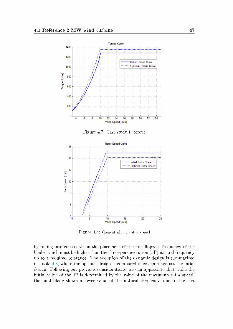
4.1 Reference 2 MW wind turbine 47
Figure 4.7: Case study 1: torque
Figure 4.8: Case study 1: rotor speed
by taking into consideration the placement of the rst apwise frequency of theblade, which must be higher than the three-per-revolution (3P) natural frequencyup to a required tolerance. The evolution of the dynamic design is summarizedin Table 4.8, where the optimal design is compared once again against the intialdesign. Following our previous considerations, we can appreciate that while theinitial value of the 3P is determined by the value of the maximum rotor speed,the nal blade shows a lower value of the natural frequency, due to the fact
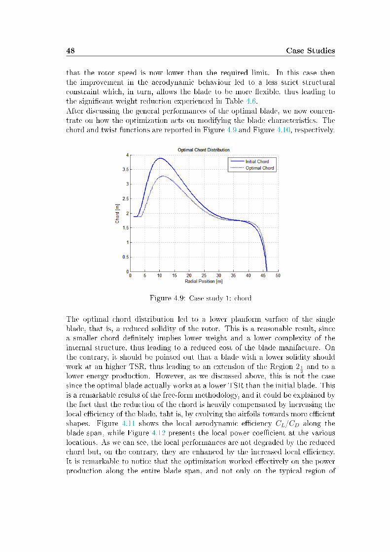
48 Case Studies
that the rotor speed is now lower than the required limit. In this case thenthe improvement in the aerodynamic behaviour led to a less strict structuralconstraint which, in turn, allows the blade to be more exible, thus leading tothe signicant weight reduction experienced in Table 4.6.After discussing the general performances of the optimal blade, we now concen-trate on how the optimization acts on modifying the blade characteristics. Thechord and twist functions are reported in Figure 4.9 and Figure 4.10, respectively.
Figure 4.9: Case study 1: chord
The optimal chord distribution led to a lower planform surface of the singleblade, that is, a reduced solidity of the rotor. This is a reasonable result, sincea smaller chord denitely implies lower weight and a lower complexity of theinternal structure, thus leading to a reduced cost of the blade manifacture. Onthe contrary, it should be pointed out that a blade with a lower solidity shouldwork at an higher TSR, thus leading to an extension of the Region 2 1
2and to a
lower energy production. However, as we discussed above, this is not the casesince the optimal blade actually works at a lower TSR than the initial blade. Thisis a remarkable results of the free-form methodology, and it could be explained bythe fact that the reduction of the chord is heavily compensated by increasing thelocal eciency of the blade, taht is, by evolving the airfoils towards more ecientshapes. Figure 4.11 shows the local aerodynamic eciency CL/CD along theblade span, while Figure 4.12 presents the local power coecient at the variouslocations. As we can see, the local performances are not degraded by the reducedchord but, on the contrary, they are enhanced by the increased local eciency.It is remarkable to notice that the optimization worked eectively on the powerproduction along the entire blade span, and not only on the typical region of
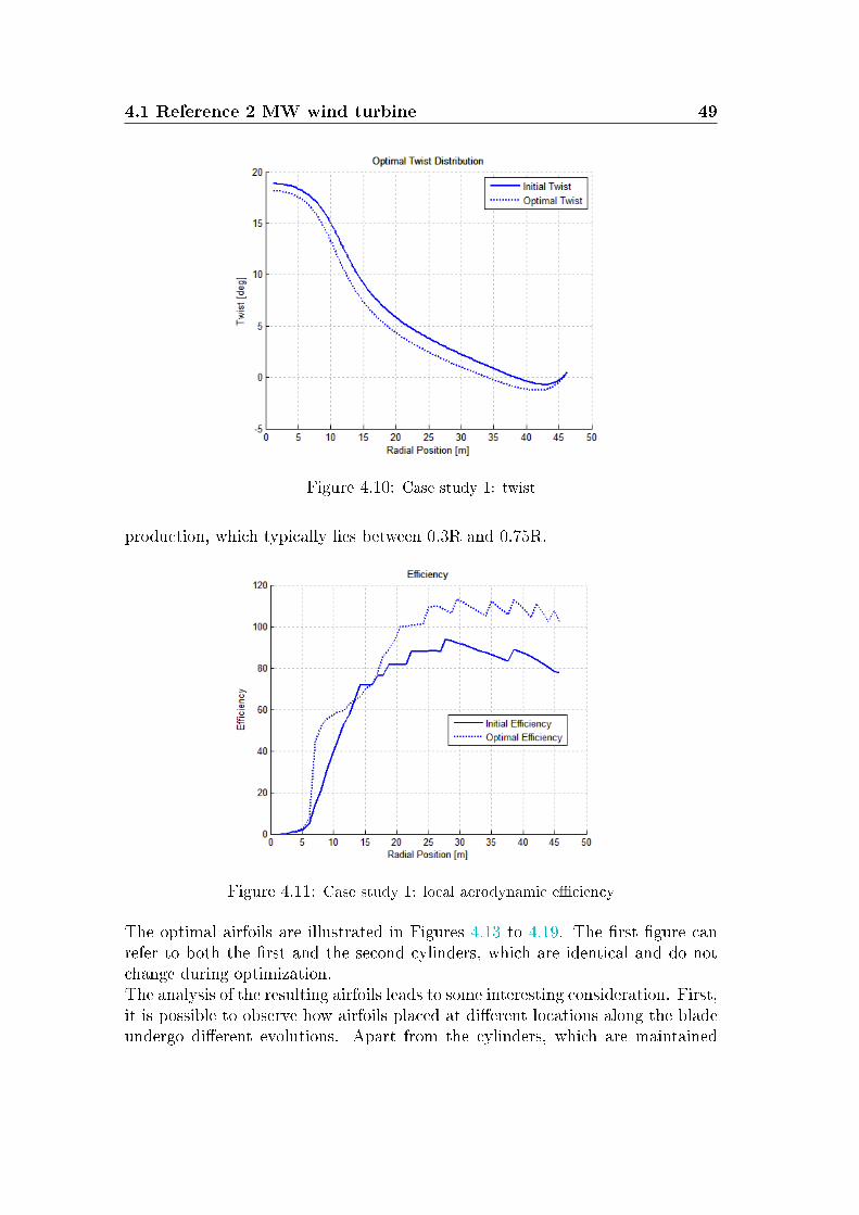
4.1 Reference 2 MW wind turbine 49
Figure 4.10: Case study 1: twist
production, which typically lies between 0.3R and 0.75R.
Figure 4.11: Case study 1: local aerodynamic eciency
The optimal airfoils are illustrated in Figures 4.13 to 4.19. The rst gure canrefer to both the rst and the second cylinders, which are identical and do notchange during optimization.The analysis of the resulting airfoils leads to some interesting consideration. First,it is possible to observe how airfoils placed at dierent locations along the bladeundergo dierent evolutions. Apart from the cylinders, which are maintained
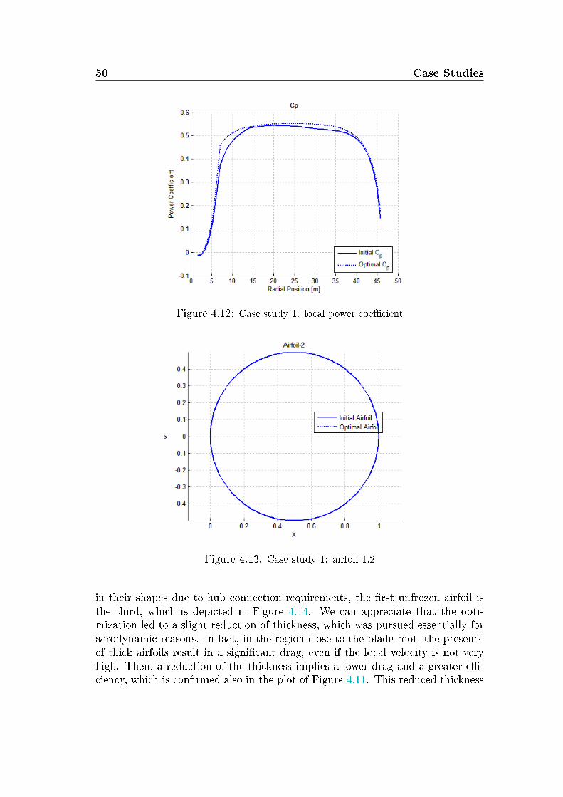
50 Case Studies
Figure 4.12: Case study 1: local power coecient
Figure 4.13: Case study 1: airfoil 1,2
in their shapes due to hub connection requirements, the rst unfrozen airfoil isthe third, which is depicted in Figure 4.14. We can appreciate that the opti-mization led to a slight reduction of thickness, which was pursued essentially foraerodynamic reasons. In fact, in the region close to the blade root, the presenceof thick airfoils result in a signicant drag, even if the local velocity is not veryhigh. Then, a reduction of the thickness implies a lower drag and a greater e-ciency, which is conrmed also in the plot of Figure 4.11. This reduced thickness
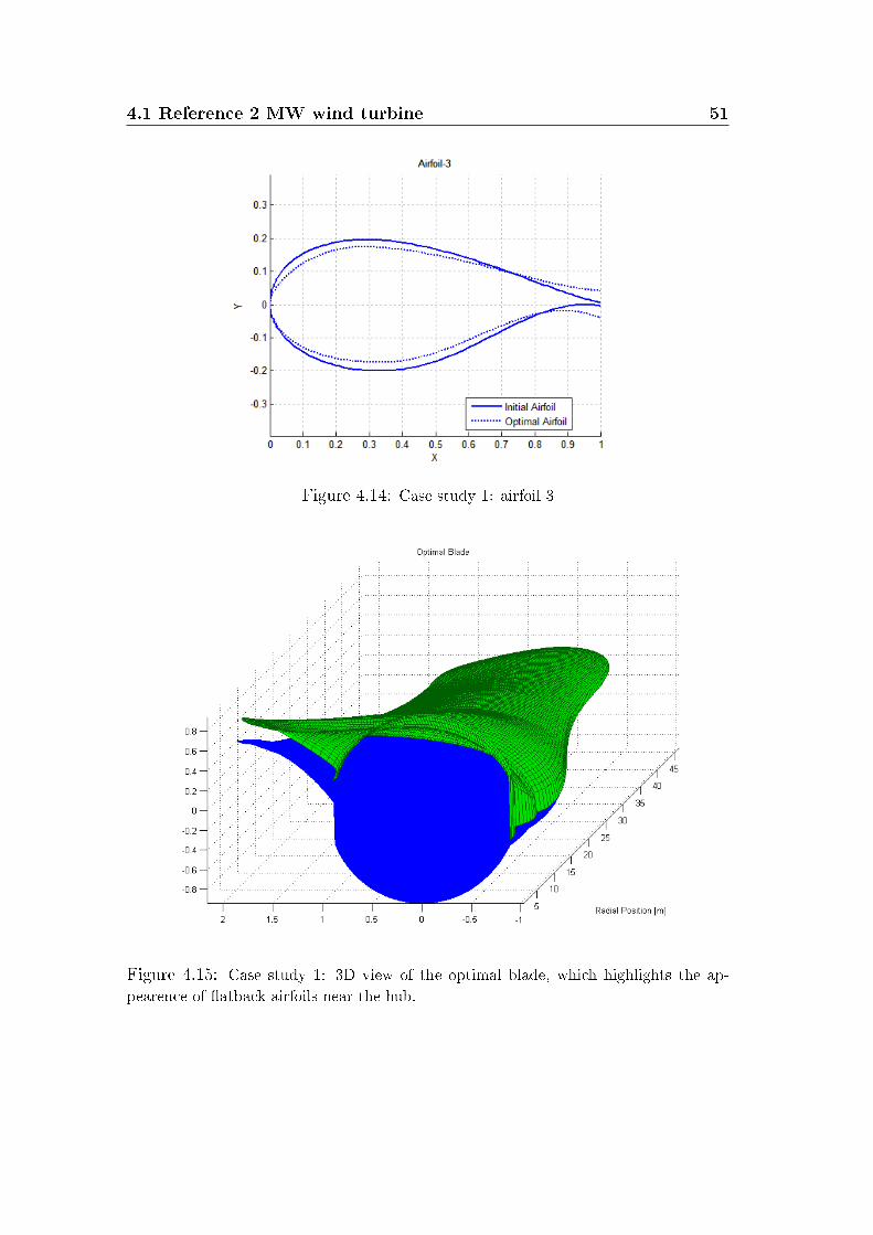
4.1 Reference 2 MW wind turbine 51
Figure 4.14: Case study 1: airfoil 3
Figure 4.15: Case study 1: 3D view of the optimal blade, which highlights the ap-
pearence of atback airfoils near the hub.
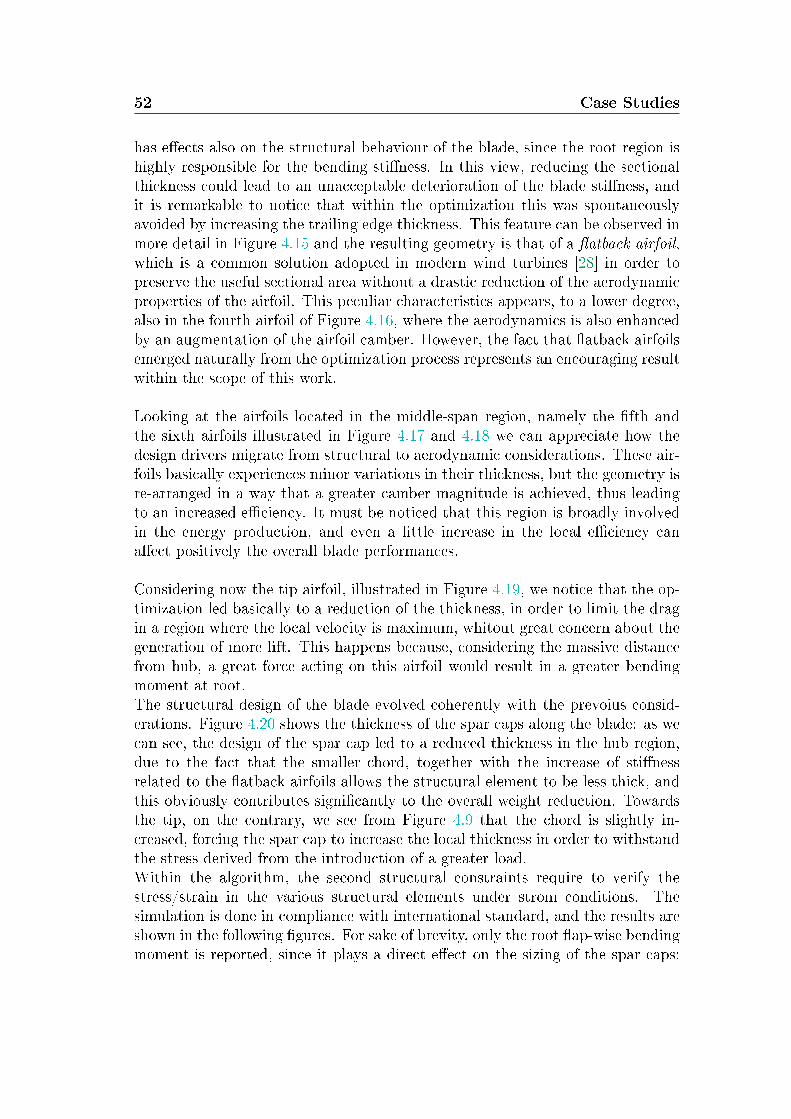
52 Case Studies
has eects also on the structural behaviour of the blade, since the root region ishighly responsible for the bending stiness. In this view, reducing the sectionalthickness could lead to an unacceptable deterioration of the blade stiness, andit is remarkable to notice that within the optimization this was spontaneouslyavoided by increasing the trailing edge thickness. This feature can be observed inmore detail in Figure 4.15 and the resulting geometry is that of a atback airfoil,which is a common solution adopted in modern wind turbines [28] in order topreserve the useful sectional area without a drastic reduction of the aerodynamicproperties of the airfoil. This peculiar characteristics appears, to a lower degree,also in the fourth airfoil of Figure 4.16, where the aerodynamics is also enhancedby an augmentation of the airfoil camber. However, the fact that atback airfoilsemerged naturally from the optimization process represents an encouraging resultwithin the scope of this work.
Looking at the airfoils located in the middle-span region, namely the fth andthe sixth airfoils illustrated in Figure 4.17 and 4.18 we can appreciate how thedesign drivers migrate from structural to aerodynamic considerations. These air-foils basically experiences minor variations in their thickness, but the geometry isre-arranged in a way that a greater camber magnitude is achieved, thus leadingto an increased eciency. It must be noticed that this region is broadly involvedin the energy production, and even a little increase in the local eciency canaect positively the overall blade performances.
Considering now the tip airfoil, illustrated in Figure 4.19, we notice that the op-timization led basically to a reduction of the thickness, in order to limit the dragin a region where the local velocity is maximum, whitout great concern about thegeneration of more lift. This happens because, considering the massive distancefrom hub, a great force acting on this airfoil would result in a greater bendingmoment at root.The structural design of the blade evolved coherently with the prevoius consid-erations. Figure 4.20 shows the thickness of the spar caps along the blade: as wecan see, the design of the spar cap led to a reduced thickness in the hub region,due to the fact that the smaller chord, together with the increase of stinessrelated to the atback airfoils allows the structural element to be less thick, andthis obviously contributes signicantly to the overall weight reduction. Towardsthe tip, on the contrary, we see from Figure 4.9 that the chord is slightly in-creased, forcing the spar cap to increase the local thickness in order to withstandthe stress derived from the introduction of a greater load.Within the algorithm, the second structural constraints require to verify thestress/strain in the various structural elements under strom conditions. Thesimulation is done in compliance with international standard, and the results areshown in the following gures. For sake of brevity, only the root ap-wise bendingmoment is reported, since it plays a direct eect on the sizing of the spar caps:
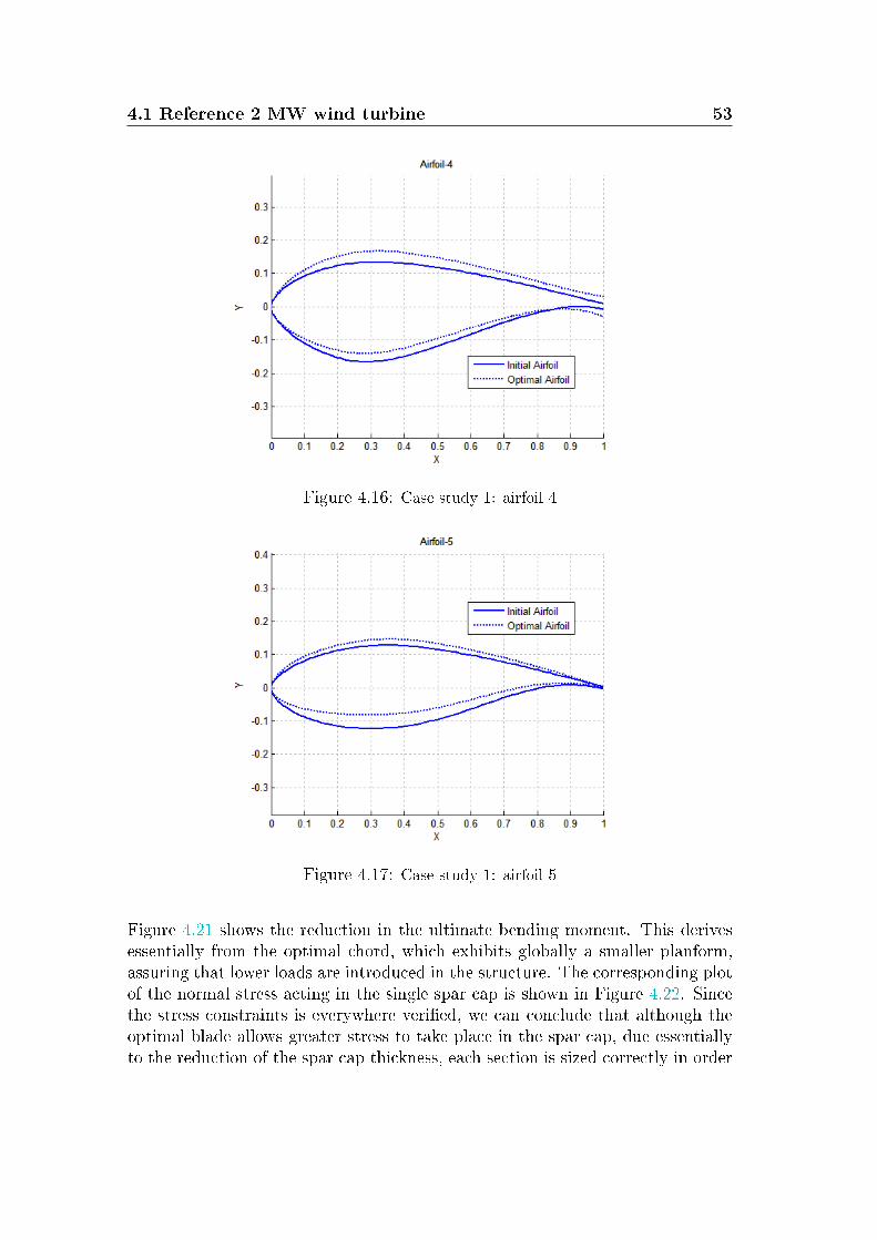
4.1 Reference 2 MW wind turbine 53
Figure 4.16: Case study 1: airfoil 4
Figure 4.17: Case study 1: airfoil 5
Figure 4.21 shows the reduction in the ultimate bending moment. This derivesessentially from the optimal chord, which exhibits globally a smaller planform,assuring that lower loads are introduced in the structure. The corresponding plotof the normal stress acting in the single spar cap is shown in Figure 4.22. Sincethe stress constraints is everywhere veried, we can conclude that although theoptimal blade allows greater stress to take place in the spar cap, due essentiallyto the reduction of the spar cap thickness, each section is sized correctly in order
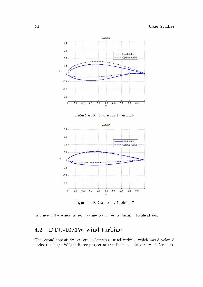
54 Case Studies
Figure 4.18: Case study 1: airfoil 6
Figure 4.19: Case study 1: airfoil 7
to prevent the stress to reach values too close to the admittable stress.
4.2 DTU-10MW wind turbine
The second case study concerns a large-size wind turbine, which was developedunder the Light Weight Rotor project at the Technical University of Denmark,

4.2 DTU-10MW wind turbine 55
Figure 4.20: Case study 1: spar cap thickness
Figure 4.21: Case study 1: root bending moment in storm conditions.
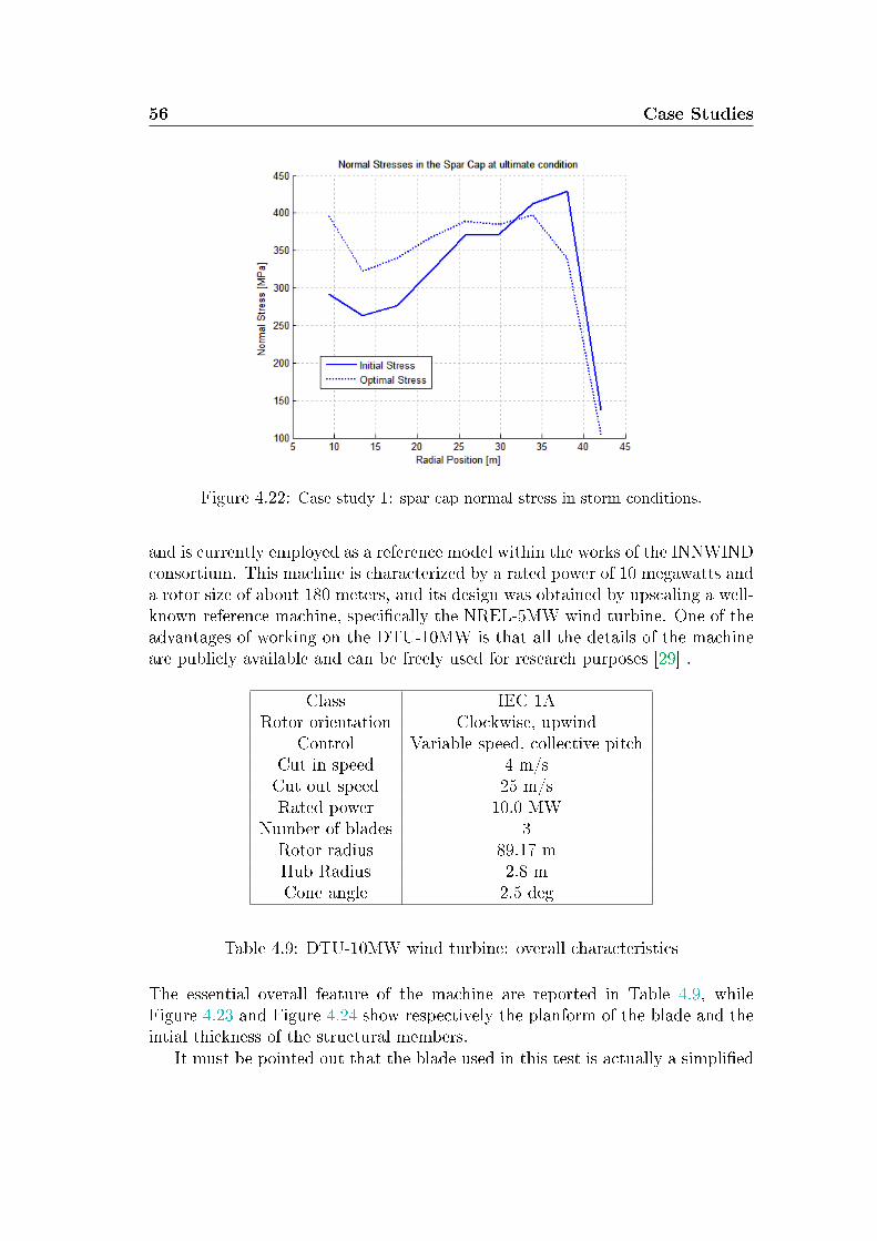
56 Case Studies
Figure 4.22: Case study 1: spar cap normal stress in storm conditions.
and is currently employed as a reference model within the works of the INNWINDconsortium. This machine is characterized by a rated power of 10 megawatts anda rotor size of about 180 meters, and its design was obtained by upscaling a well-known reference machine, specically the NREL-5MW wind turbine. One of theadvantages of working on the DTU-10MW is that all the details of the machineare publicly available and can be freely used for research purposes [29] .
Class IEC 1ARotor orientation Clockwise, upwind
Control Variable speed, collective pitchCut in speed 4 m/sCut out speed 25 m/sRated power 10.0 MW
Number of blades 3Rotor radius 89.17 mHub Radius 2.8 mCone angle 2.5 deg
Table 4.9: DTU-10MW wind turbine: overall characteristics
The essential overall feature of the machine are reported in Table 4.9, whileFigure 4.23 and Figure 4.24 show respectively the planform of the blade and theintial thickness of the structural members.
It must be pointed out that the blade used in this test is actually a simplied
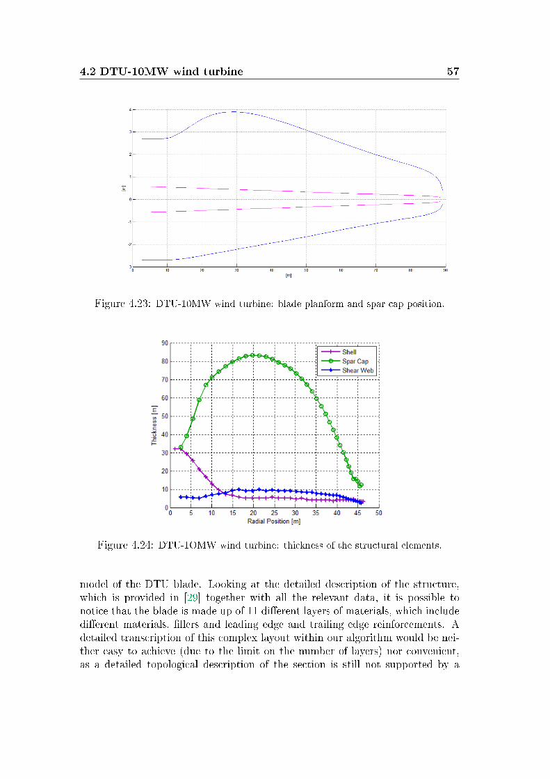
4.2 DTU-10MW wind turbine 57
Figure 4.23: DTU-10MW wind turbine: blade planform and spar cap position.
Figure 4.24: DTU-1OMW wind turbine: thickness of the structural elements.
model of the DTU blade. Looking at the detailed description of the structure,which is provided in [29] together with all the relevant data, it is possible tonotice that the blade is made up of 11 dierent layers of materials, which includedierent materials, llers and leading edge and trailing edge reinforcements. Adetailed transcription of this complex layout within our algorithm would be nei-ther easy to achieve (due to the limit on the number of layers) nor convenient,as a detailed topological description of the section is still not supported by a
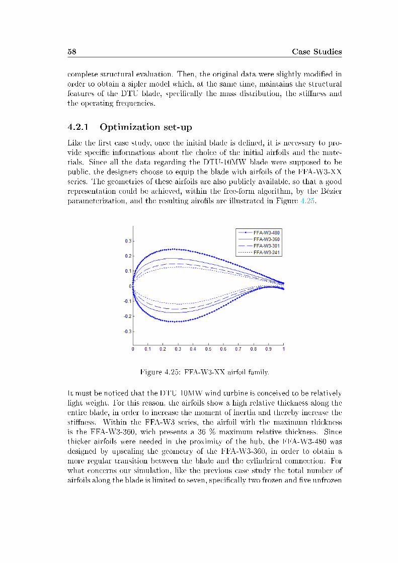
58 Case Studies
complete structural evaluation. Then, the original data were slightly modied inorder to obtain a sipler model which, at the same time, maintains the structuralfeatures of the DTU blade, specically the mass distribution, the stiness andthe operating frequencies.
4.2.1 Optimization set-up
Like the rst case study, once the initial blade is dened, it is necessary to pro-vide specic informations about the choice of the initial airfoils and the mate-rials. Since all the data regarding the DTU-10MW blade were supposed to bepublic, the designers choose to equip the blade with airfoils of the FFA-W3-XXseries. The geometries of these airfoils are also publicly available, so that a goodrepresentation could be achieved, within the free-form algorithm, by the Bézierparameterization, and the resulting airols are illustrated in Figure 4.25.
Figure 4.25: FFA-W3-XX airfoil family.
It must be noticed that the DTU-10MW wind turbine is conceived to be relativelylight weight. For this reason, the airfoils show a high relative thickness along theentire blade, in order to increase the moment of inertia and thereby increase thestiness. Within the FFA-W3 series, the airfoil with the maximum thicknessis the FFA-W3-360, wich presents a 36 % maximum relative thickness. Sincethicker airfoils were needed in the proximity of the hub, the FFA-W3-480 wasdesigned by upscaling the geometry of the FFA-W3-360, in order to obtain amore regular transition between the blade and the cylindrical comnection. Forwhat concerns our simulation, like the previous case study the total number ofairfoils along the blade is limited to seven, specically two frozen and ve unfrozen
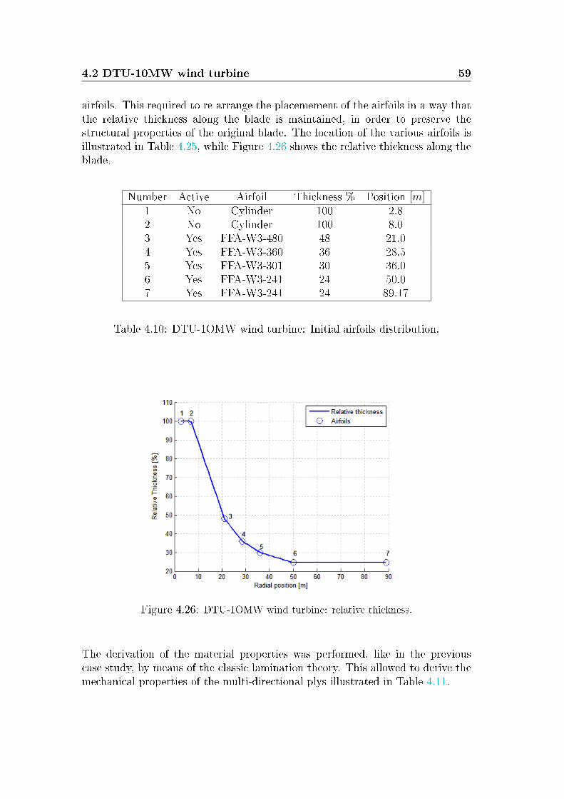
4.2 DTU-10MW wind turbine 59
airfoils. This required to re-arrange the placemement of the airfoils in a way thatthe relative thickness along the blade is maintained, in order to preserve thestructural properties of the original blade. The location of the various airfoils isillustrated in Table 4.25, while Figure 4.26 shows the relative thickness along theblade.
Number Active Airfoil Thickness % Position [m]1 No Cylinder 100 2.82 No Cylinder 100 8.03 Yes FFA-W3-480 48 21.04 Yes FFA-W3-360 36 28.55 Yes FFA-W3-301 30 36.06 Yes FFA-W3-241 24 50.07 Yes FFA-W3-241 24 89.17
Table 4.10: DTU-1OMW wind turbine: Initial airfoils distribution.
Figure 4.26: DTU-1OMW wind turbine: relative thickness.
The derivation of the material properties was performed, like in the previouscase study, by means of the classic lamination theory. This allowed to derive themechanical properties of the multi-directional plys illustrated in Table 4.11.
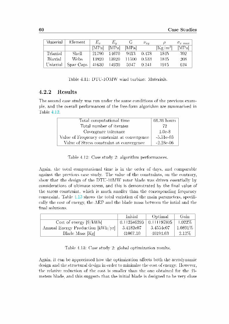
60 Case Studies
Material Element Ex Ey G νxy ρ σx max
[MPa] [MPa] [MPa] [Kg/m3] [MPa]Triaxial Shell 21790 14670 9413 0.478 1845 392Biaxial Webs 13920 13920 11500 0.533 1845 208Uniaxial Spar Caps 41630 14930 5047 0.241 1915 624
Table 4.11: DTU-1OMW wind turbine: Materials.
4.2.2 Results
The second case study was run under the same conditions of the previous exam-ple, and the overall performances of the free-form algorithm are summarized inTable 4.12.
Total computational time 66.36 hoursTotal number of iterates 72Covergence tolerance 1.0e-8
Value of Frequency constraint at convergence -5.51e-03Value of Stress constraint at convergence -2.28e-06
Table 4.12: Case study 2: algorithm performances.
Again, the total computational time is in the order of days, and comparableagainst the previous case study. The value of the constraints, on the contrary,show that the design of the DTU-10MW rotor blade was driven essentially byconsiderations of ultimate stress, and this is demonstrated by the nal value ofthe stress constraint, which is much smaller than the corresponding frequencyconstraint. Table 4.13 shows the total variation of the main parameters, speci-cally the cost of energy, the AEP and the blade mass between the intial and thenal solutions.
Initial Optimal GainCost of energy [$/kWh] 0.112346293 0.111197805 1.022%
Annual Energy Production [kWh/yr] 3.4182e07 3.4554e07 1.0891%Blade Mass [Kg] 41067.10 40194.63 2.12%
Table 4.13: Case study 2: global optimization results.
Again, it can be appreciated how the optimization aects both the aerodynamicdesign and the structural design in order to minimize the cost of energy. However,the relative reduction of the cost is smaller than the one obtained for the 45-meters blade, and this suggests that the initial blade is designed to be very close
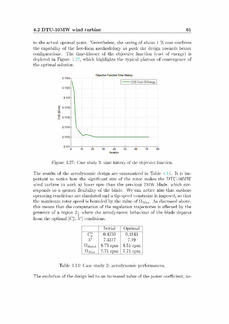
4.2 DTU-10MW wind turbine 61
to the actual optimal point. Nevertheless, the saving of about 1 % cost conrmsthe capability of the free-form methodology to push the design towards bettercongurations. The time-history of the objective function (cost of energy) isdepicted in Figure 4.27, which highlights the typical plateau of convergence ofthe optimal solution.
Figure 4.27: Case study 2: time history of the objective function.
The results of the aerodynamic design are summarized in Table 4.14. It is im-portant to notice how the signicant size of the rotor makes the DTU-10MWwind turbine to work at lower rpm than the previous 2MW blade, which cor-responds to a greater exibility of the blade. We can notice also that onshoreoperating conditions are simulated and a tip-speed constraint is imposed, so thatthe maximum rotor speed is bounded by the value of ΩMax. As discussed above,this means that the computation of the regulation trajectories is aected by thepresence of a region 2 1
2where the aerodynamic behaviour of the blade departs
from the optimal [C∗P , λ
∗] conditions.
Initial OptimalC∗
p 0.4750 0.4843λ∗ 7.3317 7.19
ΩRated 8.73 rpm 8.51 rpmΩMax 7.71 rpm 7.71 rpm
Table 4.14: Case study 2: aerodynamic performances.
The evolution of the design led to an increased value of the power coecient, to-
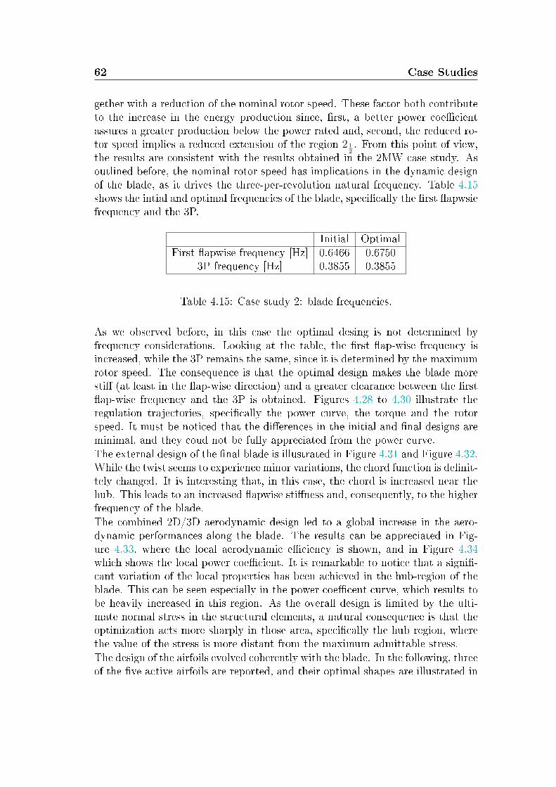
62 Case Studies
gether with a reduction of the nominal rotor speed. These factor both contributeto the increase in the energy production since, rst, a better power coecientassures a greater production below the power rated and, second, the reduced ro-tor speed implies a reduced extension of the region 2 1
2. From this point of view,
the results are consistent with the results obtained in the 2MW case study. Asoutlined before, the nominal rotor speed has implications in the dynamic designof the blade, as it drives the three-per-revolution natural frequency. Table 4.15shows the intial and optimal frequencies of the blade, specically the rst apwsiefrequency and the 3P.
Initial OptimalFirst apwise frequency [Hz] 0.6466 0.6750
3P frequency [Hz] 0.3855 0.3855
Table 4.15: Case study 2: blade frequencies.
As we observed before, in this case the optimal desing is not determined byfrequency considerations. Looking at the table, the rst ap-wise frequency isincreased, while the 3P remains the same, since it is determined by the maximumrotor speed. The consequence is that the optimal design makes the blade moresti (at least in the ap-wise direction) and a greater clearance between the rstap-wise frequency and the 3P is obtained. Figures 4.28 to 4.30 illustrate theregulation trajectories, specically the power curve, the torque and the rotorspeed. It must be noticed that the dierences in the initial and nal designs areminimal, and they coud not be fully appreciated from the power curve.The external design of the nal blade is illustrated in Figure 4.31 and Figure 4.32.While the twist seems to experience minor variations, the chord function is denit-tely changed. It is interesting that, in this case, the chord is increased near thehub. This leads to an increased apwise stiness and, consequently, to the higherfrequency of the blade.The combined 2D/3D aerodynamic design led to a global increase in the aero-dynamic performances along the blade. The results can be appreciated in Fig-ure 4.33, where the local aerodynamic eciency is shown, and in Figure 4.34which shows the local power coecient. It is remarkable to notice that a signi-cant variation of the local properties has been achieved in the hub-region of theblade. This can be seen especially in the power coecent curve, which results tobe heavily increased in this region. As the overall design is limited by the ulti-mate normal stress in the structural elements, a natural consequence is that theoptimization acts more sharply in those area, specically the hub region, wherethe value of the stress is more distant from the maximum admittable stress.The design of the airfoils evolved coherently with the blade. In the following, threeof the ve active airfoils are reported, and their optimal shapes are illustrated in
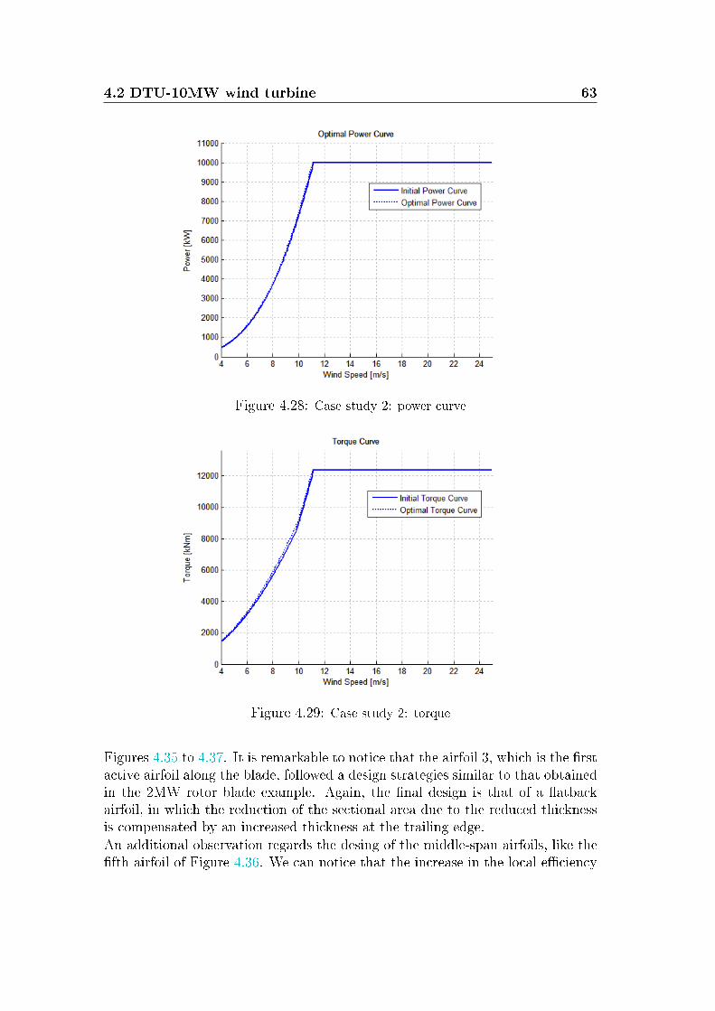
4.2 DTU-10MW wind turbine 63
Figure 4.28: Case study 2: power curve
Figure 4.29: Case study 2: torque
Figures 4.35 to 4.37. It is remarkable to notice that the airfoil 3, which is the rstactive airfoil along the blade, followed a design strategies similar to that obtainedin the 2MW rotor blade example. Again, the nal design is that of a atbackairfoil, in which the reduction of the sectional area due to the reduced thicknessis compensated by an increased thickness at the trailing edge.An additional observation regards the desing of the middle-span airfoils, like thefth airfoil of Figure 4.36. We can notice that the increase in the local eciency
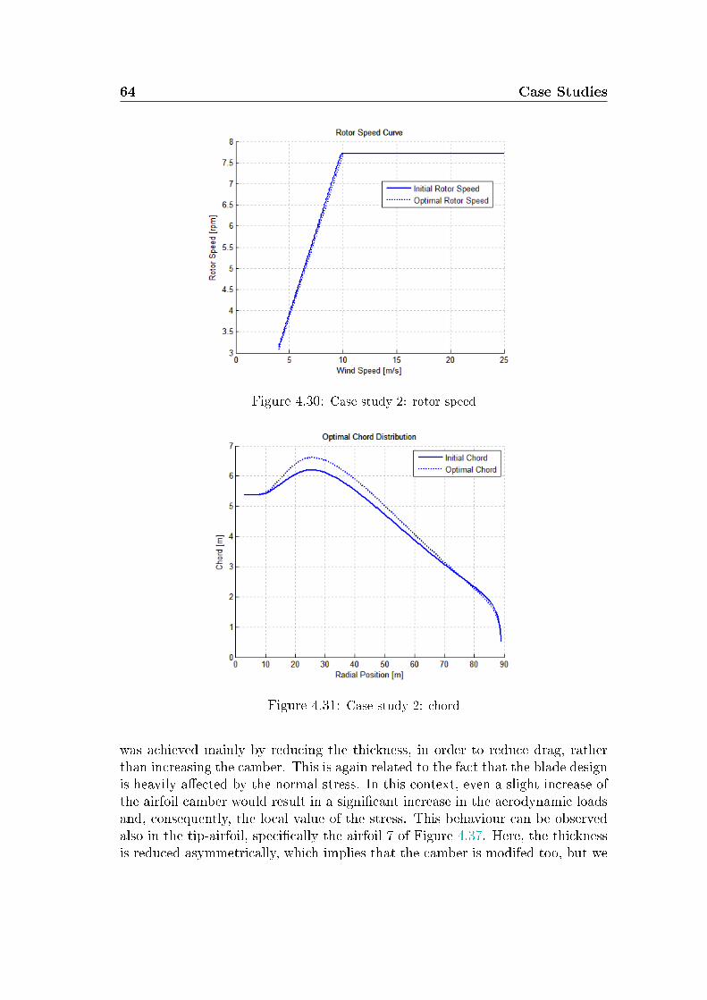
64 Case Studies
Figure 4.30: Case study 2: rotor speed
Figure 4.31: Case study 2: chord
was achieved mainly by reducing the thickness, in order to reduce drag, ratherthan increasing the camber. This is again related to the fact that the blade designis heavily aected by the normal stress. In this context, even a slight increase ofthe airfoil camber would result in a signicant increase in the aerodynamic loadsand, consequently, the local value of the stress. This behaviour can be observedalso in the tip-airfoil, specically the airfoil 7 of Figure 4.37. Here, the thicknessis reduced asymmetrically, which implies that the camber is modifed too, but we
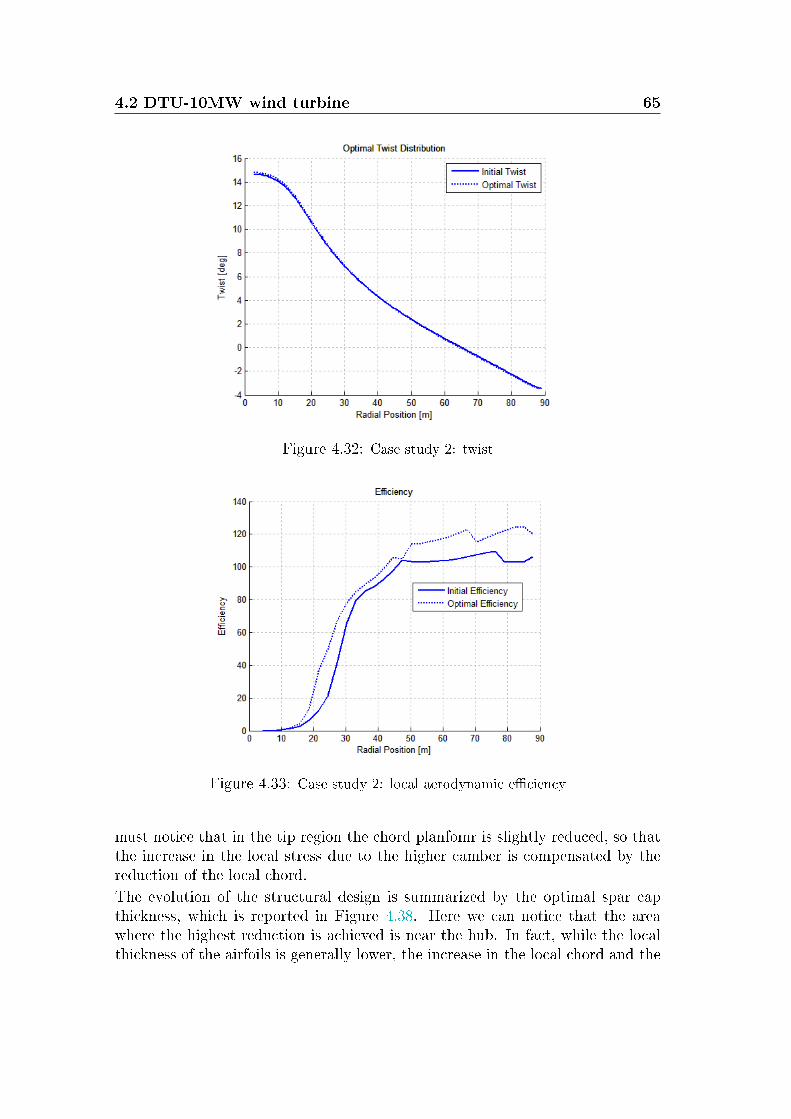
4.2 DTU-10MW wind turbine 65
Figure 4.32: Case study 2: twist
Figure 4.33: Case study 2: local aerodynamic eciency
must notice that in the tip region the chord planfomr is slightly reduced, so thatthe increase in the local stress due to the higher camber is compensated by thereduction of the local chord.
The evolution of the structural design is summarized by the optimal spar capthickness, which is reported in Figure 4.38. Here we can notice that the areawhere the highest reduction is achieved is near the hub. In fact, while the localthickness of the airfoils is generally lower, the increase in the local chord and the
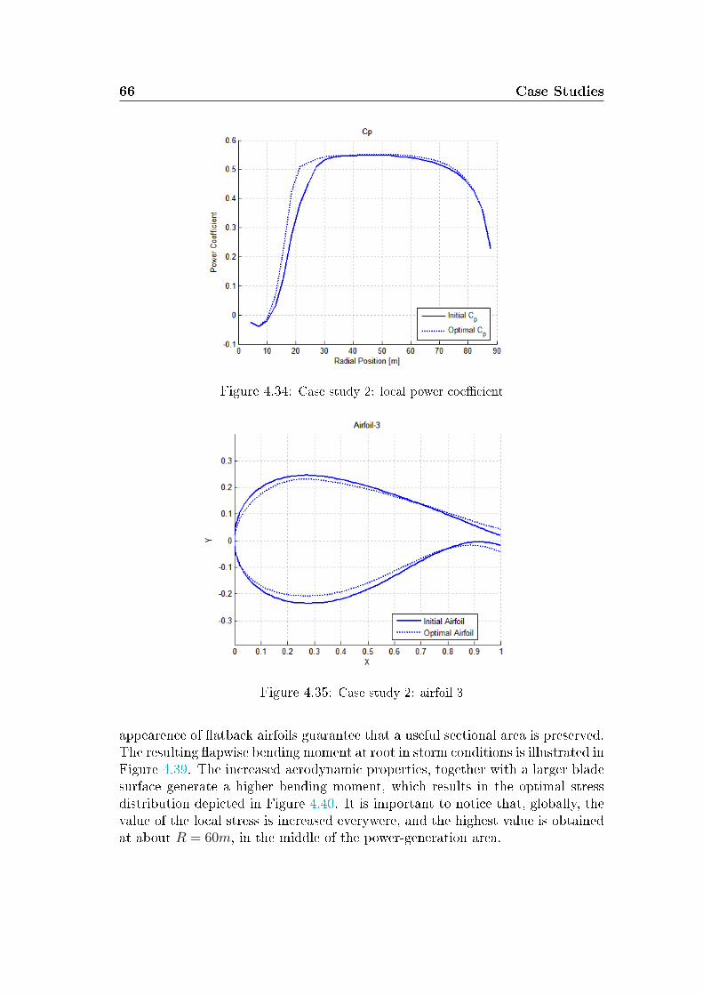
66 Case Studies
Figure 4.34: Case study 2: local power coecient
Figure 4.35: Case study 2: airfoil 3
appearence of atback airfoils guarantee that a useful sectional area is preserved.The resulting apwise bending moment at root in storm conditions is illustrated inFigure 4.39. The increased aerodynamic properties, together with a larger bladesurface generate a higher bending moment, which results in the optimal stressdistribution depicted in Figure 4.40. It is important to notice that, globally, thevalue of the local stress is increased everywere, and the highest value is obtainedat about R = 60m, in the middle of the power-generation area.
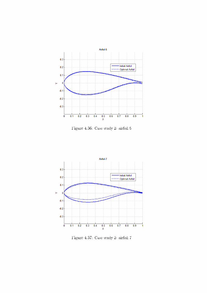
Figure 4.36: Case study 2: airfoil 5
Figure 4.37: Case study 2: airfoil 7

Figure 4.38: Case study 2: spar cap thickness
Figure 4.39: Case study 2: root bending moment in storm conditions.
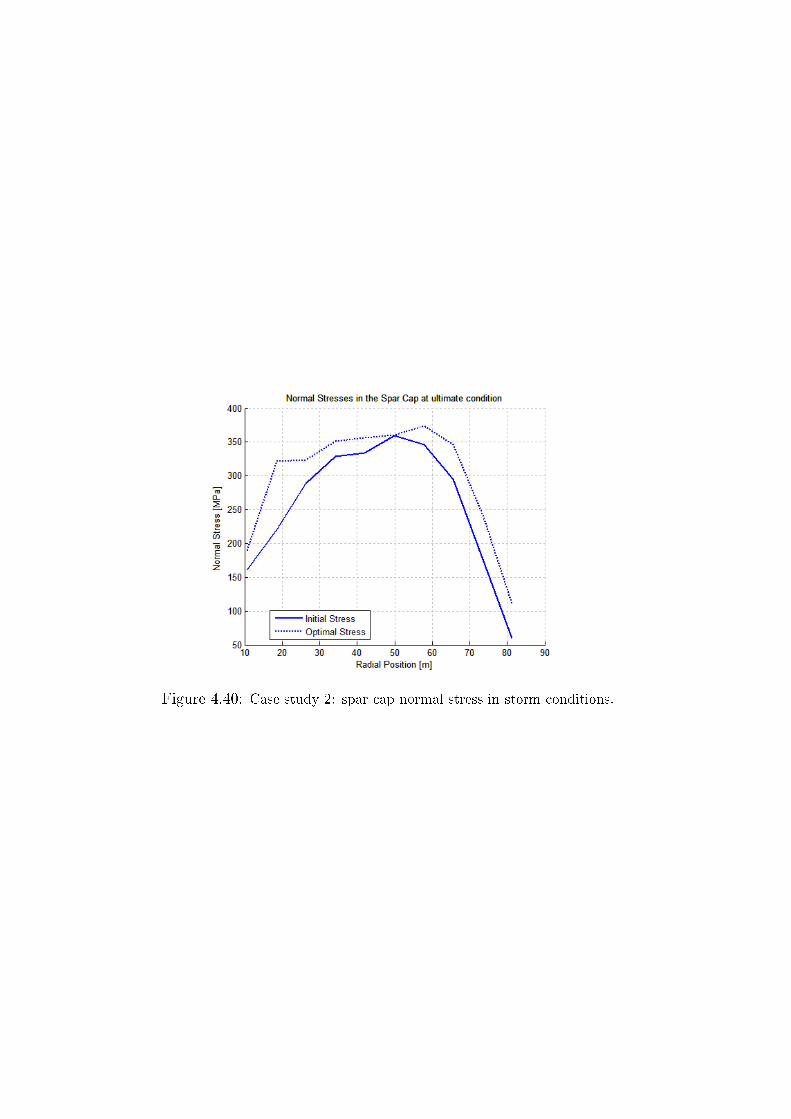
Figure 4.40: Case study 2: spar cap normal stress in storm conditions.

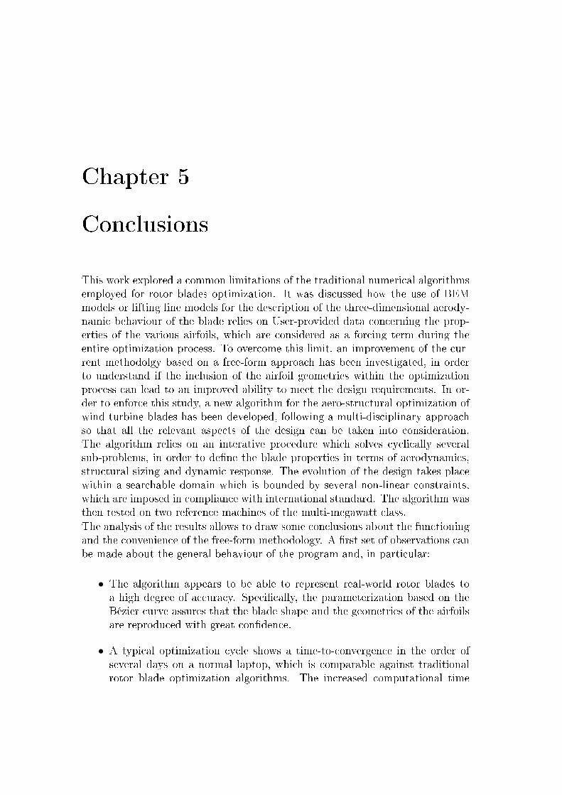
Chapter 5
Conclusions
This work explored a common limitations of the traditional numerical algorithmsemployed for rotor blades optimization. It was discussed how the use of BEMmodels or lifting line models for the description of the three-dimensional aerody-namic behaviour of the blade relies on User-provided data concerning the prop-erties of the various airfoils, which are considered as a forcing term during theentire optimization process. To overcome this limit, an improvement of the cur-rent methodolgy based on a free-form approach has been investigated, in orderto understand if the inclusion of the airfoil geometries within the optimizationprocess can lead to an improved ability to meet the design requirements. In or-der to enforce this study, a new algorithm for the aero-structural optimization ofwind turbine blades has been developed, following a multi-disciplinary approachso that all the relevant aspects of the design can be taken into consideration.The algorithm relies on an interative procedure which solves cyclically severalsub-problems, in order to dene the blade properties in terms of aerodynamics,structural sizing and dynamic response. The evolution of the design takes placewithin a searchable domain which is bounded by several non-linear constraints,which are imposed in compliance with international standard. The algorithm wasthen tested on two reference machines of the multi-megawatt class.
The analysis of the results allows to draw some conclusions about the functioningand the convenience of the free-form methodology. A rst set of observations canbe made about the general behaviour of the program and, in particular:
• The algorithm appears to be able to represent real-world rotor blades toa high degree of accuracy. Specically, the parameterization based on theBézier curve assures that the blade shape and the geometries of the airfoilsare reproduced with great condence.
• A typical optimization cycle shows a time-to-convergence in the order ofseveral days on a normal laptop, which is comparable against traditionalrotor blade optimization algorithms. The increased computational time
72 Conclusions
ascribable to the presence of unfrozen airfoils is compensated by the intrinsicsimplicity of the models.
• The algorithm is able to manage succesfully all the dierent families ofdesign variables, without incurring in bad-conditioning problems. This wasa crucial aspect of the code development and a lot of time was dedicatedto make the optimization coherent and harmonical through all the designvariables.
For what relates to the specical aspects of the free-form methodolgy, it is possibleto draw the following conclusions:
• The program works eectively even if the initial blade shows very goodperformances. We conclude that the ability to adapt the airfoils to thelocal requirements as they change during the optimization can lead to abetter design.
• The optimal design of the various airfoils pursues dierent goals dependingon the position of the airfoil along the blade. Specically, the airfoils closeto the hub region are driven by structural and stiness considerations, whilemoving towards the tip implies a greater role of the arodynamic design. Thisbehavior, which is actually typical of rotor blade design, was achieved bymeans of only general constraints, i.e. no requirements about local camberand thickness were applied.
• Some typical solutions adopted in large wind turbines emerged naturallyduring the design of the airfoils, like for example the presence of atbackairfoils near the hub and the appearence of typical S-tail in the lower surface.
Globally, we can conclude that the objectives of this work have been met. Thefree-form methodology seems to provide an improved ability to meet the designrequirements and, moreover, it allows the designer to be less specic for whatconcerns the design of the initial airfoils. As the airfoils are automatically tailoredto meet the features of the optimal blade, the onerous task of forecasting inadvance the local properties of the airfoils can be moved from the designer tothe optimization algorithm, provided that physical-meaningful constraints areimposed on the nal design.
5.1 Future developments
This work was conceived to be a preliminary study of the free-form methodology,and thus it shows some intrinsic limitations which must be addressed and pos-sibly corrected in further, more deepened, investigations. Some ideas for futuredevelopments of this work are here proposed:
5.1 Future developments 73
• In this rst version of the program, the numerical estimation of the airfoilcharacteristics is done by XFOIL. It was noticed, however, than this solverlimits its eectiveness to the pre-stall region. While this was not actuallya problem within our simple analysis, a greater eectiveness of the airfoildesign could be achieved by a better description of the near-stall and thepost-stall regions. ECN devloped for this purpose RFOIL, which is a renedversion of XFOIL with a more accurate description of the airfoil behaviourat higher angles of attacks. An example of its application in airfoil designis provided by Grasso in [11] and [12]. A possible alternative solutionscould be to replace a panel-method solver with a 2D nite element solver,in which the Naviér-Stokes equation are solved directly. An example ofthis approach was pursued by Dahl and Fuglsang for the development ofthe EllipSys2D solver [30], but its convenience within large optimizationalgorithms should be evaluated carefully.
• The set of the structural design variables in this analysis includes only thethickness of the spar cap along the blade. A rened version of the programshould allow a broader level of freedom of the structural design, throughthe introduction of additionl degrees of freedom associated with the otherstructural elements, specically the shell and the shear webs. This couldbe achieved easily by minor modications of the structural modules withinthe program and, obviously, one or more new constraints should be addedin order to take into account the phenomena which aect these structuralelements, like for example a buckling verication.
• It must be noticed that, so far, no specical requirements on the airfoilshapes have been used. This means that the airfoils evolve only under theaction of the two global structural constraints. In real world, however, thedesign of wind turbine dedicated airfoils is also aected by 2D considera-tions, for example by imposing limits on the maximum lift coecient, or byprescribing the behaviour of the boundary layer at certain angles of attack.It would be interesting to introduce such constraints in the algorithm, toverify how the optimal design changes.
• The use of WT Perf as BEM solver was decided for sake of simplicity.Although it proved to be fast and reliable it only supports elementary,turbulence-free scenarios. There are more sophisticated softwares whichcould be used in order to grant a more detailed description of the windeld, for example the popular AeroDyn, which is generally coupled withTurbSim for the simulation of turbulent conditions. It would be very inter-esting to improve the program with these modules but, in this case, a moredetailed description of the airfoil stall must be assured, in order to allowthe use of the Beddoe's dynamic stall models included in AeroDyn [31].
74 Conclusions
• It would be interesting, also, to test the free-form methodolgy within ahigh-complexity optimization algorithm, with full support of the DLCs andfull dynamic simulation. This kind of analysis could rely on the Cp-Max
solver developed at Politecnico, and would allow to study the impact of thefree-form airfoil design on fatigue and Actuator Duty Cycles under all theconditions required by international certication guidelines.
• Since a gradient-base optimization method is employed, the dependencieson the initial condition should be evaluated carefully. At present, a param-teric analysis is running in order to estimate the ability of the program toobtain unique optimal solutions for dierent intial conditions, and the re-sults will be presented at the next EWEA conference in Barcelona, on March2014. If a strong dependency on the initial blade will be demonstrated, apossible countermeasure should be to introduce a hybrid approach, basedon the coupling between a global optimization algorithm with the SQPemployed in this study. This should bring to a greater robustness of theprogram.
Bibliography
[1] E. T. G. Bot and O. Ceyhan. Blade Optimisation Tool User's manual. ECN-E09-092. 2011. url: http://www.ecn.nl/docs/library/report/2009/e09092.pdf.
[2] C.L. Bottasso, F. Campagnolo, and A. Croce. Computational Procedures forthe Multi-Disciplinary Constrained Optimization of Wind Turbines. DIA-SR 10-02. Dipartimento di Ingegneria Aerospaziale, Politecnico di Milano,Milano, Italy, 2010.
[3] M. Drela. Pros and Cons of Airfoil Optimization. In: Frontiers of Com-putational Fluid Dynamics (1998).
[4] G. Venter. Review of Optimization Techniques. In: Encyclopedia of AerospaceEngineering (2010). Ed. by John Wiley and Sons.
[5] J.L. Zhou, A.L. Tits, and C.T. Lawrence. User's guide for FFSQP version3.7: A fortran code for solving optimization programs, possibly minimax,with general inequality constraints and linear equality constraints, generat-ing feasible iterates. 1997.
[6] Paul T. Boggs and Jon W. Tolle. Sequential Quadratic Programming. 1995.
[7] L. Fingersh, M. Hand, and A. Laxson. Wind Turbine Design cost and Scal-ing Model. NREL/TP-500-40566. Golden, Colorado, USA, 2006.
[8] Anonymus.Wind Turbines Part 1: Design Requirements. International Stan-dard IEC 61400-1. 2005.
[9] Germanischer Lloyd. Guideline for the Certication of Wind Turbines.Hamburg, Germany, 2010.
[10] A.L. Rogers and J.F. Manwell. Wind Turbine Acoustic Noise. Golden, Col-orado, USA, 2002.
[11] Francesco Grasso. Development of Thick Airfoils for wind Turbines. In:50th AIAA Aerospace Sciences Meeting. Vol. AIAA 2012. Nashville, TN,USA, 2012, p. 0236.
[12] Francesco Grasso. Design and Optimization of Tidal turbine airfoil. In:29th AIAA Applied Aerodynamics Conference. Vol. AIAA 2011. Honolulu,HI, USA, 2011, p. 3816.
76 BIBLIOGRAPHY
[13] R. Mukesh, K. Lingadurai, and A. Muruganandham. Application of PAR-SEC Geometry Representation to General Airfoil for Aerodynamic Opti-mization. In: Lecture Notes in Information Technology 10 (2012), pp. 5560.
[14] M. Drela. XFOIL 6.94 User Guide. 2001.
[15] L.A. Viterna and R.D. Corrigan. Fixed pitch rotor performance of largehorizontal axis wind turbines. In: DOE/NASA Workshop on large horizon-tal axis wind turbines. Cleveland, Ohio, USA, 1981.
[16] Francesco Grasso. Usage of Numerical Optimization in Wind Turbine Air-foil Design. In: 28th AIAA Applied Aerodynamics Conference. Chicago, IL,USA, 2010.
[17] Ira H. A. Abbott. Theory of Wing Sections: Including a Summary of AirfoilData. New York: Courier Dover, 1959.
[18] Morten Hartvig Hansen. Aeroelastic instability problems for wind tur-bines. In: Wind Energy 10.6 (2007), pp. 551577. issn: 1095-4244.
[19] A. D. Platt and M. L. Buhl. WT Perf User Guide for Version 3.05.00.Golden, Colorado, USA, 2012.
[20] Tony Burton et al. Wind Energy Handbook. Wiley, 2011.
[21] C.L. Bottasso et al. Structural Optimization of Wind Turbine Rotor Bladesby Multi-Level Sectional/Multibody/3DFEM Analysis. DIA-SR 12-01. Di-partimento di Ingegneria Aerospaziale, Politecnico di Milano, Milano, Italy,2012.
[22] G. Bir. User's guide to BModes (Software for computing rotating beam cou-pled modes. NREL/TP-500-39133. National Renewable Energy Laboratory,Golden,Colorado, 2005.
[23] J.P. Blasques and R. Bitsch. User's Manual for BECAS - a cross sectionanalysis tool for anisotropic and inho-mogeneous beam sections of arbitrarygeometry. DTU, Roskilde, Denmark, 2012.
[24] G. L. Ghiringhelli and P. Mantegazza. Linear, straight and untwistedanisotropic beam section properties from solid nite elements. In: Com-posites Eng 4.12 (1994), pp. 12251239.
[25] V. Giavotto, M. Borri, et al. Anisotropic Beam Theory and Applications.In: Computers and Structures 16.1-4 (1983), pp. 403413.
[26] Franck Bertagnolio et al. Wind Turbine Airfoil Catalogue. Roskilde, Den-mark: Risø National Laboratory, 2001.
[27] C. Chamis. Simpied composite cicromechanics equations for hygral, ther-mal and mechanical properites. NASA Technical Memorandum 83320. LewisResearch cCenter, Cleveland, Ohio, 1983.
BIBLIOGRAPHY 77
[28] J.A. Paquette and P.S. Veers. Increased Strength in Wind Turbine Bladesthrough Innovative Structural Design. In: European Wind Energy Confer-ence and Exhibition. Milan, Italy, 2007.
[29] C. et al. Bak. Description of the DTU 10 MW Reference wind turbine. DTUWind Energy Report-I-0092. 2013.
[30] K.S. Dahl and P. Fuglsang. Design of the wind turbine airfoil family Risø-A-XX. Risø-R-1024(EN). 1998.
[31] P.J. Moriarty and A.C. Hansen. AeoDyn theory manual. NREL/TP-500-36881. 2005.
[32] Andrew Ning, Rick Damiani, and Patrick Moriarty. Objectives and Con-straints for Wind Turbine Optimization. In: 51st AIAA Aerospace Sci-ences Meeting including the New Horizons Forum and Aerospace Exposi-tion. Grapevine, Texas, USA, 2013.
[33] Jin Chen et al. Optimization design of blade shapes for wind turbines. In:Jixie Gongcheng Xuebao 46.3 (2010), pp. 131134. issn: 0577-6686.
[34] Danny Sale. HARP-Opt User's Guide. 2010.
[35] Kevin Maki, Ricardo Sbragio, and Nickolas Vlahopoulos. System design ofa wind turbine using a multi-level optimization approach. In: RenewableEnergy 43 (2012), pp. 101110.
[36] Fujio Yamaguchi. Curves and surfaces in computer aided geometric design.Springer, 1988, pp. IX, 1378. isbn: 978-0-387-17449-5.
[37] Gustave P. Corten. Flow Separation on Wind Turbine Blades. Utrecht, TheNetherlands: Proefschrift Universiteit Utrecht, 2001.
[38] J. Fazil and V. Jayakumar. Investigation of airfoil prole Design UsingReverse Engineering Bezier Curve. In: ARPN Journal of Engineering andApplied Sciences 6.7 (2011).
[39] J. Jonkman et al. Denition of a 5-MW Reference Wind Turbine for O-shore System Development. NREL/TP-500-38060. Golden, Colorado, USA,2009.
[40] M. Jureczko, M. Pawlak, and A. Mezyk. Optimisation of wind turbineblades. In: Journal of Materials Processing Technology 167 (2005), pp. 463471.
[41] G.C. Larsen et al.Modal Analysis of Wind Turbine Blades. RisøR1181(EN).Roskilde, Denmark, 2002.
[42] J. L. Tangler and D. M. Somers. NREL Airfoils Families for HAWTs.NREL/TP-442-7109. Golden, Colorado, USA, 1995.
78 BIBLIOGRAPHY
[43] Henrik Broen Pedersen and Ole Jesper Dahl Kristensen. Applied ModalAnalysis of Wind Turbine Blades. Risø-R-1388(EN). Roskilde, Denmark,2003.
[44] Dan M. Somers. Design and Experimental Results for the S805 Airfoil.NREL/SR-440-6917. Golden, Colorado, USA, 1997.
[45] W.A. Timmer and R.P.J.O.M. van Rooij. Summary of the Delft UniversityWind Turbine Dedicated Airfoils. AIAA-2003-0352. Delft, the Netherlands,2003.
[46] J. Tangler and David J. Kocurek. Wind Turbine Post-Stall Airfoil Perfor-mance Characteristics Guidelines for Blade-Element Momentum Methods.NREL/CP-500-36900. Golden, Colorado, 2004.
[47] A. Baumgart. A Mathematical Model for Wind Turbine Blades. In: Jour-nal of Sound and Vibrations 251.1 (2002), pp. 112.
[48] P. Fuglsang and H. Madsen. Optimization Method for Wind Turbine Ro-tors. In: Journal of Wind Engineering and Industrial Aerodynamics 80(1999), pp. 191206.