Policy teachingthrough reward function learning

A thesis presented

by

Haoqi Zhang

to

Computer Science and Economics

in partial fulfillment of the honors requirementsfor the degree ofBachelor of Arts

Harvard UniversityCambridge, Massachusetts

April 3rd, 2007

Policy teaching through reward function learning

Abstract

Many situations arise in which an interested party wishes to provide incentives to

an agent so that the agent’s modified behavior meets some goal external (but possi-

bly related) to the agent. The problem is difficult because the reward function gov-

erning the agent’s behavior is often complex and unknown to the interested party.

We study this problem in sequential decision-making tasks modeled by Markov

Decision Processes. We develop novel algorithms that learn the reward function of

an agent and use learned information to provide incentives for the agent to meet

an external goal. We conduct experiments motivated by a real world scenario, and

show that we can generally find incentives to modify an agent’s behavior as de-

sired in a small number of iterations. In addition to studying a technical problem,

this work has applications in education, economics, and multi-agent systems.

iii

Acknowledgments

I thank David Parkes for being a great mentor. His advice, direction, and sup-

port have not only made this senior thesis possible, but have helped me grow as

a researcher, a teacher, and a person. The weekly meetings helped, a lot. I thank

Jerry Green for his support and guidance, and for helping me realize the signif-

icance of this work in an economics context. I thank Daniel Wood and Jonathan

Kolstad for reading drafts of this work and providing useful feedback. I thank

Alex Allain for taking an interest in this work and for pushing me to think about

the work in realistic settings. I thank Andrei Munteanu for helping me visualize

space. I thank Pavithra Harsha for her help on programming formulations.

Lastly, I thank Laura and my parents.

All errors are my own.

iv

Contents

Title page . . . . . . . . . . . . . . . . . . . . . . . . . . . . . . . . . . . . . . iAbstract . . . . . . . . . . . . . . . . . . . . . . . . . . . . . . . . . . . . . . . iiiAcknowledgments . . . . . . . . . . . . . . . . . . . . . . . . . . . . . . . . ivTable of Contents . . . . . . . . . . . . . . . . . . . . . . . . . . . . . . . . . v

1 Introduction 11.1 Contributions . . . . . . . . . . . . . . . . . . . . . . . . . . . . . . . . 31.2 Related Work . . . . . . . . . . . . . . . . . . . . . . . . . . . . . . . . 41.3 Outline . . . . . . . . . . . . . . . . . . . . . . . . . . . . . . . . . . . . 8

2 Policy Teaching with Known Rewards 92.1 Markov Decision Process . . . . . . . . . . . . . . . . . . . . . . . . . . 9

2.1.1 Definition . . . . . . . . . . . . . . . . . . . . . . . . . . . . . . 102.1.2 Properties . . . . . . . . . . . . . . . . . . . . . . . . . . . . . . 12

2.2 Policy Teaching with Known Rewards . . . . . . . . . . . . . . . . . . 142.2.1 The Interested Party’s Problem . . . . . . . . . . . . . . . . . . 142.2.2 Setup . . . . . . . . . . . . . . . . . . . . . . . . . . . . . . . . . 172.2.3 Domains without an Expert . . . . . . . . . . . . . . . . . . . . 192.2.4 Domains with an Expert . . . . . . . . . . . . . . . . . . . . . . 22

3 Policy Teaching with Unknown Rewards 263.1 Inverse Reinforcement Learning . . . . . . . . . . . . . . . . . . . . . 26

3.1.1 Definition . . . . . . . . . . . . . . . . . . . . . . . . . . . . . . 273.1.2 Properties . . . . . . . . . . . . . . . . . . . . . . . . . . . . . . 30

3.2 Policy Teaching with Unknown Rewards . . . . . . . . . . . . . . . . 333.2.1 Setup . . . . . . . . . . . . . . . . . . . . . . . . . . . . . . . . . 333.2.2 Elicitation Method . . . . . . . . . . . . . . . . . . . . . . . . . 353.2.3 Domains with an Expert . . . . . . . . . . . . . . . . . . . . . . 393.2.4 Domains without an Expert . . . . . . . . . . . . . . . . . . . . 473.2.5 Elicitation Objective Function . . . . . . . . . . . . . . . . . . . 52

v

4 Experiments 614.1 Experiments . . . . . . . . . . . . . . . . . . . . . . . . . . . . . . . . . 61

4.1.1 Experimental Setup . . . . . . . . . . . . . . . . . . . . . . . . . 614.1.2 Setting Parameters . . . . . . . . . . . . . . . . . . . . . . . . . 614.1.3 Testing Example . . . . . . . . . . . . . . . . . . . . . . . . . . 63

4.2 Results . . . . . . . . . . . . . . . . . . . . . . . . . . . . . . . . . . . . 664.2.1 Domain with an Expert . . . . . . . . . . . . . . . . . . . . . . 664.2.2 Domain without an Expert . . . . . . . . . . . . . . . . . . . . 714.2.3 Summary . . . . . . . . . . . . . . . . . . . . . . . . . . . . . . 74

5 Discussion 755.1 Applications . . . . . . . . . . . . . . . . . . . . . . . . . . . . . . . . . 75

5.1.1 Real-World Applications . . . . . . . . . . . . . . . . . . . . . . 755.1.2 Multi-agent Systems . . . . . . . . . . . . . . . . . . . . . . . . 78

5.2 Critique . . . . . . . . . . . . . . . . . . . . . . . . . . . . . . . . . . . . 815.2.1 Parameters and Constraints . . . . . . . . . . . . . . . . . . . . 815.2.2 Assumptions . . . . . . . . . . . . . . . . . . . . . . . . . . . . 835.2.3 Expressiveness . . . . . . . . . . . . . . . . . . . . . . . . . . . 845.2.4 The Elicitation Process . . . . . . . . . . . . . . . . . . . . . . . 865.2.5 Long Term Effects . . . . . . . . . . . . . . . . . . . . . . . . . 88

5.3 Open Questions and Future Research . . . . . . . . . . . . . . . . . . 90

6 Conclusion 916.1 Brief Review . . . . . . . . . . . . . . . . . . . . . . . . . . . . . . . . . 916.2 Conclusion . . . . . . . . . . . . . . . . . . . . . . . . . . . . . . . . . . 93

Bibliography 94

vi

Chapter 1

Introduction

There are many scenarios in which an interested party wishes for an agent to be-

have in a certain way. An elementary school teacher wants his student to solve

arithmetic problems correctly. Parents want their child to go home after school. A

firm wants a consumer to make a purchase. In many cases, the behavior desired by

the interested party may differ from the actual behavior of the agent. The student

may solve the problems incorrectly, the child may go to the park instead of going

home, and the consumer may not be interested in the product being sold.

For the interested party to affect the behavior of an agent, the interested party

can often provide incentives to modify the agent’s preferences so as to induce a

behavior that meets the external goal. A teacher can offer candy to a student for

solving problems correctly, parents can allow more TV time if their child comes

home immediately, and a firm can use advertisements and discounts to entice the

consumer to make a purchase.

However, there are a number of underlying obstacles that make it difficult for

the interested party to modify the agent’s behavior as desired. Some of the major

issues include:

• The amount of incentive that can be given may be limited.

A teacher may only have so much candy; parents may only wish to give so

much TV time; a firm may only wish to spend so much on advertisements

1

and discounts.

• Providing incentives after completion of tasks may not be sufficient.

An agent will be most interested in immediate rewards, and offering incen-

tives later will be discounted by the agent. A student may value finishing

the problems quickly over receiving candy after the homework gets graded;

a child may prefer playing at the park now to watching TV later; a consumer

may prefer immediate discounts over mail-in rebates.

• The agent’s preferences may be complex.

The agent’s behavior is a sequence of actions in a complex domain, where

a decision now affects subsequent decisions. Figuring out where and when

to offer incentives can be difficult, especially when getting the agent to per-

form as desired may require additional incentives in many states. In some

situations, the agent’s actions may be unobservable in certain states.

• The agent’s preferences may be unknown to the interested party.

One cause of this may be that the agent wishes not to share his preferences

with the interested party. Another cause is that it may be difficult for the

agent to write down his preferences. The student would be hard-pressed to

write down relative weights for different alternatives; the child cannot write

down how much he values going to the park, and a consumer cannot easily

write down how much something is worth to him. While the agents’ actions

are governed by their inherent preferences, writing down such information

accurately is extremely difficult, especially in complex domains.

Despite these obstacles, there is considerable interest in understanding how to

provide incentives to affect the behavior of agents. This thesis aims to answer the

question of policy teaching: Given an agent facing a sequential decision-making

task, how can an interested party provide minimal incentives to modify the agent’s

behavior to meet a goal external to the agent?

2

In addition to the numerous real-world applications, this work is motivated by

applications to multi-agent systems, where methods for learning the participants’

unknown preferences and providing incentives to modify the agents’ behaviors

can aid in the design of better systems and implementation of socially beneficial

outcomes.

1.1 Contributions

We study the policy teaching problem under the Markov Decision Process (MDP)

framework. We tackle the policy teaching problem with known and unknown re-

wards, both in domains with an expert and domains without. For policy teaching

with unknown rewards, we use techniques of inverse reinforcement learning [16]

as a starting point to develop a novel method for elicitating the preferences of

an agent using only observations of the agent’s policy before and after added in-

centives. Based on this method, we develop algorithms that iteratively learn the

reward function of an agent, and use learned information to provide incentives to

meet an external goal. We prove bounds on the number of elicitation rounds our

algorithms require before returning a solution to the policy teaching problem if

one exists.

The algorithms we have developed are general elicitation methods that can al-

low for any elicitation strategy. We discuss possible objective functions for the elici-

tation process, and introduce tractable heuristics that can significantly decrease the

number of elicitation rounds necessary in practice. We perform experiments on our

algorithms with these heuristics in a simulated domain inspired by a real-world

example. Our results show that even with unknown rewards, our algorithms can

generally find incentives to modify an agent’s behavior as desired within a small

number of iterations.

Finally, we provide a sketch of applications of policy teaching to real-world

3

problems and to the study of multi-agent systems. We address the major critiques

of our work, and discuss extensions and open questions for future research.

1.2 Related Work

Our work is interdisciplinary in nature, and related to research in economics and

computer science. The closest analogue is in economics, where contract theory

and principal-agent theory study the question of how a principal can provide in-

centives in the form of contracts to align the interest of the agent with that of the

principal. Principal-agent problems often deal with hidden information (adverse

selection) and hidden action (moral hazard), and contract theory deals with this by

using incentive compatibility constraints such that the agent will pick the contract

that is optimal for the principal and then act in a desired way. Bolton and Dewa-

tripont [4] provide a thorough coverage of this area of study, as does Laffront and

Martimort [13].

The questions addressed by principal-agent theory is similar to the policy teach-

ing question. As in principal-agent theory, we consider self-interested agents who

perform with respect to their own preferences and not the preferences of the in-

terested party. In our work, we can view the interested party as a principal who

provides incentives (a contract) to drive the agent toward behaving as desired.

Furthermore, in considering domains with unknown preferences, we study an ad-

verse selection problem and attempt to come up with an optimal contract despite

the hidden information. Like dynamic adverse selection in contract theory, we

consider settings with repeated interactions between the interested party and the

agent.

Despite these similarities, there are a number of fundamental differences in the

domains considered and assumptions made. First, an agent’s preferences in se-

quential decision tasks are highly multidimensional; generalizing to multidimen-

4

sional domains has been difficult in contract theory. Second, we assume that the

states and actions of the agent are observable, and thus do not study moral hazard

problems. Third, we consider a repeated setting in which the agent is myopically

rational; the agent will not attempt to distort the interested party’s beliefs about

his preferences by purposely performing suboptimally. This is different than dy-

namic adverse selection, where the agent is strategic and may act to deliberately

withhold information from the principal. Finally, the use of incentive constraints

in domains with hidden information in contract theory generally results in less ef-

ficient allocations than under complete information. Our work attempts to learn

the hidden preferences of the agent to enable us to provide better contracts.

In computer science, our work is inspired by applications of inverse reinforce-

ment learning to apprenticeship learning. Abbeel and Ng [1] studied this problem

by extracting a reward function from a human expert, and using the reward func-

tion to govern the behavior of a machine agent. They conducted experiments in

a driving setting, where their machine agent avoided obstacles while driving by

performing based on a reward function extracted from demonstrations by a hu-

man expert. By learning a reward function instead of just mimicking policies, their

agent was able to perform well even when traffic conditions were modified.

Part of our work can be seen as an extension to AI apprenticeship learning, in

that we aim to teach a human agent to behave like the human expert. In doing

so, our work faces numerous challenges that were not present in Abbeel and Ng’s

work. First, in teaching a human agent, we cannot redefine the agent’s reward

function at will; we may only provide incentives to induce the agent to behave

according to both his inherent reward function and the provided incentives. Sec-

ond, given the limits on the amount of incentives that can be provided, it may not

be possible for the agent to perform like the expert. Finding the best alternative

can be computationally difficult. Finally, because we must provide incentives, the

size of the incentives must be in line with the reward function of the agent. For

5

example, if the agent is buying a car, providing a five dollar discount would not

be sufficient, but we may nevertheless make this mistake if we do not learn both

the shape and size of the agent’s reward. In Abbeel and Ng’s work, any reward

function within the solution space was sufficient, out of which they picked the one

that would generalize well.

As our work is concerned with learning the preferences of the agent, it is re-

lated to the literature on preference elicitation. The literature is vast and we will

not review it all here, but it is worth pointing out some similarities and differences

in comparison with our work. Often, preference elicitation is performed by ask-

ing a series of queries [7, 8, 17] about the agent’s preferences, based on which the

elicitor gathers information to place bounds on the utility function of the agent. In

our work, we do not query for the agent’s preferences directly, but instead perform

indirect elicitation by using observations of the agent’s responses to incentives and

the principle of revealed preference to place bounds on the agent’s utility func-

tions1. While indirect elicitation techniques based on the principles of revealed

preferences are nothing new (in fact, techniques in inverse reinforcement learning

is an example), such techniques are typically passive; they are applied to observed

behaviors, and are unconcerned with generating new evidence based on which to

make further inferences about the agent’s preferences. Our elicitation method of-

fers incentives to an agent, and actively generates new evidence about the agent’s

reward function based on his response to the provided incentives. To our knowl-

edge, this approach has not been previously studied in the literature, and may be

useful for learning preferences in a wide range of settings.

Preference elicitation is commonly seen as a costly process, and the literature

often adapts criteria to balance this cost with the benefits of the elicited informa-

tion. In our work, we show that our elicitation algorithms can adapt the commonly

used minimax regret decision criteria [25] as an objective function for the elicitation

1For a survey of the economics literature on revealed preferences, see Varian’s article [24].

6

process. However, computing this objective function is intractable in our domain,

leading us to focus primarily on developing tractable heuristics that aim to reduce

the length of the elicitation process in practice.

Other areas of computer science have also made use of preference elicitation

techniques. For example, work by Gajos and Weld [12] on personalizable user

interfaces used preference elicitation to learn an accurate cost function based on

which to generate user interfaces. More recently, Gajos, Long, and Weld [11] ex-

tended their work to generate custom user interfaces for users with disabilities.

Their work differs from ours in that their elicitation method queries the agent’s

preferences directly, and in that they are not concerned with sequential decision

tasks.

The policy teaching problem bears resemblance to imitation learning [18, 19,

23], which aims to aid the transfer of knowledge from an expert to a student in

reinforcement learning. Our work differs in that we assume the agent is a planner

who already knows how to perform optimally with respect to his preferences, but

that the interested party may still wish to provide incentives to affect the agent’s

optimal behavior. Furthermore, a student in imitation learning needs to reason

about how similar the expert is to him; in our setting, the student cares only about

his own behavior and does not reason about the expert’s behavior.

Finally, our work is inspired by the numerous applications of computer science

and economics techniques to real-world problems like those which motivate our

work. There is work applying artificial intelligence techniques to education [2].

There is work that uses a Markov Decision Process to design a computerized guid-

ance system that determines when and how to provide prompts to a user with

dementia [3]. Works in these areas have been successful, and we believe could

benefit from better understanding of the agent’s preferences.

7

1.3 Outline

In Chapter 2, we introduce Markov Decision Processes and study the policy teach-

ing problem with observable rewards. In Chapter 3, we introduce Inverse Re-

inforcement Learning and study the policy teaching problem with unknown re-

wards. In Chapter 4, we present the results of our experiments. In Chapter 5, we

discuss potential applications, critiques, extensions, and open questions for future

research.

8

Chapter 2

Policy Teaching with Known Rewards

In this chapter we introduce Markov Decision Process (MDP) as a framework for

modeling sequential decision tasks, and use this framework to discuss the policy

teaching problem with known rewards.

2.1 Markov Decision Process

As we have shown in our introduction, many of the examples we have considered

are sequential decision-making tasks, where decisions made now can affect deci-

sions in the future. In modeling such tasks, we are interested in a framework that

can capture the following:

• Different states of the world.

We want to know if the child at school, at the park, or at home.

• Rewards for different states.

How much does the child value being at the park? Being at home?

• Actions moving agents from state to state.

Walking east brings the child from one place to another.

• Uncertainty in an action’s outcome.

The child may attempt to walk east but end up walking south.

9

• Discounting.

Future rewards count less than immediate rewards.

• Variable time period.

We are interested in what the child does, and do not want to be limited to

only considering what the child does in a fixed number of steps.

The infinite-horizon Markov Decision Process framework fulfills our criteria quite

nicely. Not only does the framework allow us to model complex domains, it also

has an elegant, intuitive formalism.

2.1.1 Definition

Definition 1. An infinite horizon MDP is a model M = {S, A,R, P, γ}:

• S is the set of states in the world.

• A is the set of possible actions.

• R is a function from S to R, where R(s) is the reward in state s.

• P is a function from S × A × S to [0, 1], where P (s, a, s′) is the probability of

transitioning from the current state s to state s′ upon taking action a.

• γ is the discount factor from (0, 1).

Notice that the reward and transition probabilities are dependent only on the

current state and not on the history of states visited. This is known as the Markov

assumption. We may also specify a start state sstart to denote the initial state of the

agent. From this state the agent takes a series of actions astart, a1, a2, . . . , visit-

ing states sstart, s1, s2, . . . while receiving rewards R(sstart), γR(s1), γ2R(s2), · · · .

We can express the agent’s utility as the sum of discounted rewards, R(sstart) +∑∞k=1 γkR(sk).

10

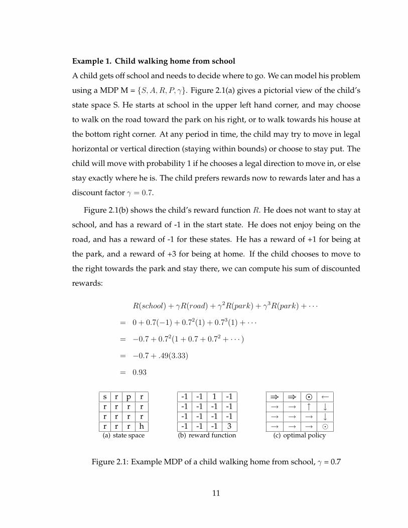
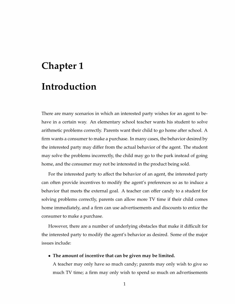
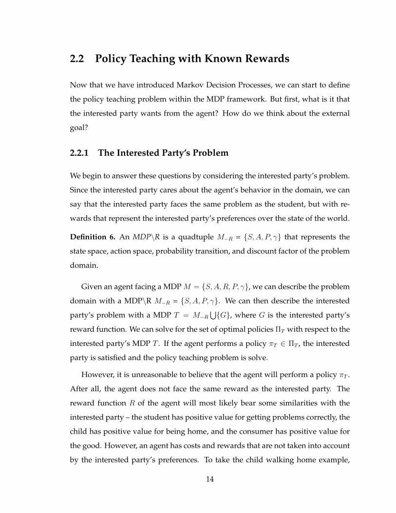
Example 1. Child walking home from school

A child gets off school and needs to decide where to go. We can model his problem

using a MDP M = {S, A,R, P, γ}. Figure 2.1(a) gives a pictorial view of the child’s

state space S. He starts at school in the upper left hand corner, and may choose

to walk on the road toward the park on his right, or to walk towards his house at

the bottom right corner. At any period in time, the child may try to move in legal

horizontal or vertical direction (staying within bounds) or choose to stay put. The

child will move with probability 1 if he chooses a legal direction to move in, or else

stay exactly where he is. The child prefers rewards now to rewards later and has a

discount factor γ = 0.7.

Figure 2.1(b) shows the child’s reward function R. He does not want to stay at

school, and has a reward of -1 in the start state. He does not enjoy being on the

road, and has a reward of -1 for these states. He has a reward of +1 for being at

the park, and a reward of +3 for being at home. If the child chooses to move to

the right towards the park and stay there, we can compute his sum of discounted

rewards:

R(school) + γR(road) + γ2R(park) + γ3R(park) + · · ·

= 0 + 0.7(−1) + 0.72(1) + 0.73(1) + · · ·

= −0.7 + 0.72(1 + 0.7 + 0.72 + · · · )

= −0.7 + .49(3.33)

= 0.93

s r p rr r r rr r r rr r r h(a) state space

-1 -1 1 -1-1 -1 -1 -1-1 -1 -1 -1-1 -1 -1 3

(b) reward function

⇒ ⇒ � ←→ → ↑ ↓→ → → ↓→ → → �(c) optimal policy

Figure 2.1: Example MDP of a child walking home from school, γ = 0.7

11

2.1.2 Properties

Now that we have defined the MDP formalism, we turn to look at the agent’s deci-

sion problem. We assume that the agent is rational, in that the agent maximizes his

expected utility by choosing actions to maximize the expected sum of discounted

rewards. The agent’s decisions form a policy, which describes the agent’s actions in

every state of the world at any time period. We restrict our attention to stationary

policies:1

Definition 2. A stationary policy is a function π from states to actions, such that π(s)

is the action the agent executes in state s, regardless of the time period.

Given a stationary policy π, we can define the value function V π:

Definition 3. A value function V π from S to R represents the total sum of discounted

rewards from state s to the infinite future under policy π:

V π(s) = R(s) + γ∑s′∈S

P (s, s′, π(s))V π(s′) (2.1)

Notice that the value function is defined recursively, such that the value in state s is

the reward in state s plus the discounted expected value from possible transitioned

to states s′ while following policy π.

Definition 4. An optimal policy π∗ chooses the action that maximizes the value func-

tion in every state:

V π∗(s) = max

a∈AR(s) + γ

∑s′∈S

P (s, s′, a)V π∗(s′),∀s ∈ S (2.2)

For each action a considered in state s, we define the value of taking action a and

following the optimal policy in future states as the Q function:

1We can do this without loss of generality in the sense that an agent will always have an optimalstationary policy as an optimal policy. We can easily extend our model to allow for other policies,but the current model should suffice for our purposes.

12

Definition 5. The Q function from S × A to R satisfies the following equation:

Q(s, a) = R(s) + γ∑s′∈S

P (s, s′, a)V π∗(s′),∀s ∈ S (2.3)

We can rewrite Equation 2.2 in terms of the Q function:

V π∗(s) = max

a∈AQ(s, a) (2.4)

One way to solve this set of equations is to use a linear program (LP). Consider

the following formulation:

minV,Q

∑s

c(s) · V (s) (2.5)

subject to:

V (s) ≥ Q(s, a) ∀s ∈ S, a ∈ A (2.6)

Q(s, a) ≥ R(s) + γ∑s′∈S

P (s, s′, a)V (s′) ∀s ∈ S, a ∈ A (2.7)

where c(s) are positive constants such that∑

s c(s) = 1.2 The constraints ensure

that V (s) is an upper bound for the value of the MDP [20], and the objective pushes

V (s) down to be exactly that value. Using the solved Q values, the optimal policy

π∗ is given by π∗(s) ∈ arg maxa Q(s, a). Notice that there may be more than one

optimal policy, since there may be more than one action that is optimal for a given

state.

Figure 2.1(c) shows an optimal policy for the child in Example 1. The arrows in

the state denote the direction the child will move in for each state, and � denotes

the child choosing to stay put in the state. We see that starting from school in the

upper left corner, the child will walk right towards the park, and choose to stay at

the park and not go home. While the child gets a larger reward for being home,

the costs on the path towards home are too high for the reward to be worth going

for, unless the child was already within two steps of home.2Actually, any positive numbers will work for c(s). Having them sum to 1 allows for c(s) to

represent a probability distribution over possible start states.

13

2.2 Policy Teaching with Known Rewards

Now that we have introduced Markov Decision Processes, we can start to define

the policy teaching problem within the MDP framework. But first, what is it that

the interested party wants from the agent? How do we think about the external

goal?

2.2.1 The Interested Party’s Problem

We begin to answer these questions by considering the interested party’s problem.

Since the interested party cares about the agent’s behavior in the domain, we can

say that the interested party faces the same problem as the student, but with re-

wards that represent the interested party’s preferences over the state of the world.

Definition 6. An MDP\R is a quadtuple M−R = {S, A, P, γ} that represents the

state space, action space, probability transition, and discount factor of the problem

domain.

Given an agent facing a MDP M = {S, A,R, P, γ}, we can describe the problem

domain with a MDP\R M−R = {S, A, P, γ}. We can then describe the interested

party’s problem with a MDP T = M−R

⋃{G}, where G is the interested party’s

reward function. We can solve for the set of optimal policies ΠT with respect to the

interested party’s MDP T . If the agent performs a policy πT ∈ ΠT , the interested

party is satisfied and the policy teaching problem is solve.

However, it is unreasonable to believe that the agent will perform a policy πT .

After all, the agent does not face the same reward as the interested party. The

reward function R of the agent will most likely bear some similarities with the

interested party – the student has positive value for getting problems correctly, the

child has positive value for being home, and the consumer has positive value for

the good. However, an agent has costs and rewards that are not taken into account

by the interested party’s preferences. To take the child walking home example,

14

the child may undervalue being home (as compared to the parents), have costs for

walking on the road, and have rewards for being at the park. Given these factors,

the child’s default optimal policy is unlikely to simultaneously be a policy that

performs optimally for the parents’ problem.

We can denote the agent’s personal costs and rewards by a function C, and

write the agent’s reward as R = G + C. The interested party can provide an incen-

tive function ∆, such that the agent’s modified reward function R′ = G + C + ∆.

We define the notion of admissible incentive function to express the limits on the

incentives an interested party provides:

Definition 7. An incentive function ∆ is admissible if it satisfies the following con-

straints:

• ∆(s) ≥ 0,∀s ∈ S

We want to restrict our attention to only positive incentives, that is, we do not

allow the interested party to use punishment to affect the agent’s behavior.

•∑

s ∆(s) ≤ Dmax

The amount of incentives the interested party is willing to provide is bounded

by Dmax.3

One seemingly simple thing for the interested party to do is just to provide a

motivating reward ∆ = −C to induce an agent reward R′ = G based on which the

agent will behave as the interested party desired. However, there are a couple of

problems with this idea. First, if the agent has any positive personal reward for

some state s such that C(s) > 0, then the interested party would have to provide

a punishment ∆(s) < 0, which violates the admissible condition. Second,∑

s ∆(s)

3This constraint is not exactly accurate. Since an agent may visit a state more than once, limitson the incentives provided in states should be dependent on the number of times each state isvisited. Since we do not know a priori what states the agent will visit and how many times,

∑s ∆(s)

provides a rough estimate of the amount of incentives that will be provided. We can get a betterestimate by including history into the state space, but this requires an exponential blowup of thestate space. We will return to this issue in Chapter 5.

15

may be greater than the maximum motivation Dmax that the interested party is

willing to provide. Finally, in the teaching, parenting, and shopping examples that

motivate our work, we would imagine that the interested party hopes that an agent

eventually “absorbs” the provided incentives; that is, the agent over time internal-

izes the provided incentive and performs as the interested party desires without

having to provide any (or much) external incentives. If ∆ is large, the agent may

not be able to motivate himself enough to internalize the provided incentive.4

Nevertheless, there may be some cases in which the interested party may be

able to provide a ∆ = −C. More generally, the interested party aims to provide

incentives such that the agent performs well under the interested party’s problem,

even if the agent’s policy is not optimal under the interested party’s MDP T . We

see an example of this below.

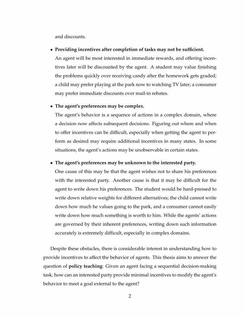
0 0 -1 00 0 0 00 0 0 00 0 0 3

(a) parents

-1 -1 1 -1-1 -1 -1 -1-1 -1 -1 -1-1 -1 -1 3

(b) child

0 -1 1 1-1 -1 -1 0-1 -1 -1 -1-1 -1 -1 3

(c) child after motivation

⇒ ⇓ ↓ ↓→ ⇒ ⇒ ⇓→ → → ⇓→ → → �

⇒ ⇒ � ←→ → ↑ ↓→ → → ↓→ → → �

⇒ ⇒ ⇒ ⇓→ → → ⇓→ → → ⇓→ → → �

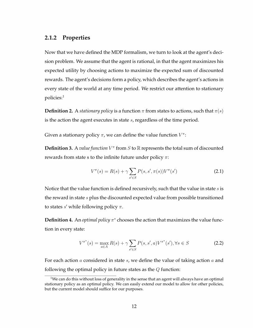
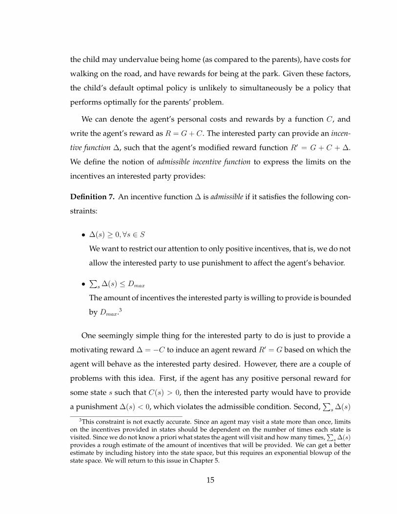
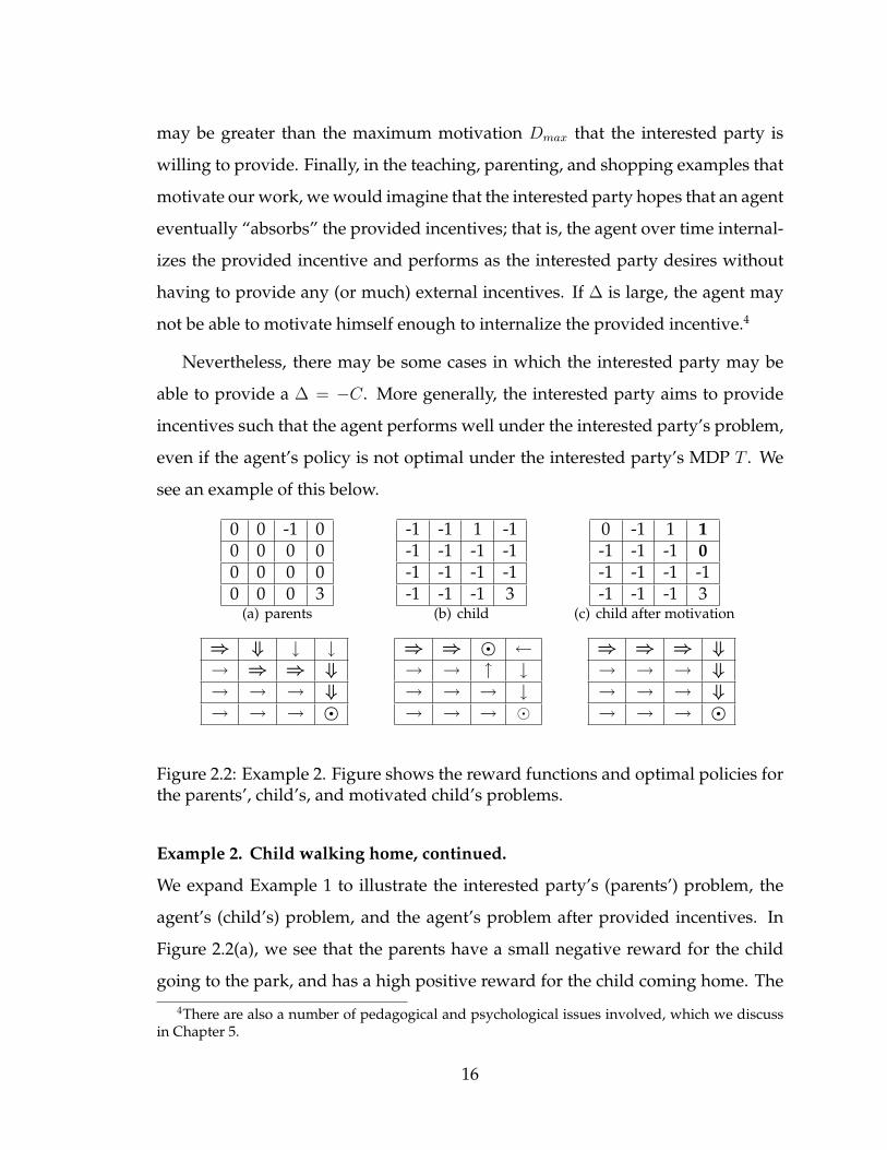
Figure 2.2: Example 2. Figure shows the reward functions and optimal policies forthe parents’, child’s, and motivated child’s problems.

Example 2. Child walking home, continued.

We expand Example 1 to illustrate the interested party’s (parents’) problem, the

agent’s (child’s) problem, and the agent’s problem after provided incentives. In

Figure 2.2(a), we see that the parents have a small negative reward for the child

going to the park, and has a high positive reward for the child coming home. The

4There are also a number of pedagogical and psychological issues involved, which we discussin Chapter 5.

16

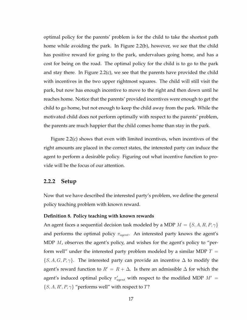
optimal policy for the parents’ problem is for the child to take the shortest path

home while avoiding the park. In Figure 2.2(b), however, we see that the child

has positive reward for going to the park, undervalues going home, and has a

cost for being on the road. The optimal policy for the child is to go to the park

and stay there. In Figure 2.2(c), we see that the parents have provided the child

with incentives in the two upper rightmost squares. The child will still visit the

park, but now has enough incentive to move to the right and then down until he

reaches home. Notice that the parents’ provided incentives were enough to get the

child to go home, but not enough to keep the child away from the park. While the

motivated child does not perform optimally with respect to the parents’ problem,

the parents are much happier that the child comes home than stay in the park.

Figure 2.2(c) shows that even with limited incentives, when incentives of the

right amounts are placed in the correct states, the interested party can induce the

agent to perform a desirable policy. Figuring out what incentive function to pro-

vide will be the focus of our attention.

2.2.2 Setup

Now that we have described the interested party’s problem, we define the general

policy teaching problem with known reward.

Definition 8. Policy teaching with known rewards

An agent faces a sequential decision task modeled by a MDP M = {S, A,R, P, γ}

and performs the optimal policy πagent. An interested party knows the agent’s

MDP M , observes the agent’s policy, and wishes for the agent’s policy to “per-

form well” under the interested party problem modeled by a similar MDP T =

{S, A,G, P, γ}. The interested party can provide an incentive ∆ to modify the

agent’s reward function to R′ = R + ∆. Is there an admissible ∆ for which the

agent’s induced optimal policy π′agent with respect to the modified MDP M ′ =

{S, A,R′, P, γ} “performs well” with respect to T ?

17

We see that translating the problem statement to the MDP setting is fairly nat-

ural. Notice that the conditions on π′agent performing well in the interested party’s

problem are purposely left out of Definition 8, and will be specified for the spe-

cific domains we consider. In the problem definition we have restricted the agent’s

modified rewards to be additive; this is easily generalizable to any affine transfor-

mation over the incentive function.5 To focus our attention, we make the following

additional assumptions:

Assumption 1. The state and action spaces are finite.

Assumption 2. R(s) ≤ Rmax ∀s ∈ S

The agent’s reward function is bounded.

These assumptions are not very restrictive. More difficult to satisfy is the inter-

ested party having knowledge of the agent’s reward function. Nevertheless, cer-

tain conditions can make this possible. First, because we are in a repeated setting,

the interested party may have learned this information over time, i.e. from us-

ing a direct preference elicitation mechanism to query for the agent’s preferences.

Second, the interest party may have learned the agent’s reward function based on

observations of the agent’s behavior in multiple settings. Third, in some cases, the

agent may be able articulate his preferences and the interested party may learn of

these preferences from the agent sharing the information directly. One possible ex-

ample of this is shopping for clothing, where a consumer may let the salesperson

know of her values for different types of clothing.

Techniques for solving for policy teaching in settings with known rewards will

still be useful when we delve into settings with unknown rewards. But how do

we approach this problem at all? To induce the agent to perform a policy π′ that

performs well in the interested party’s problem, the interested party must find

5The interested party would have to know the affine transformation. In domains we consider inwhich agents have repeated interactions with the interested party, the interested party can learn thetransformation over time. Furthermore, the effect of incentives on an agent is likely to be (almost)independent of state, which simplifies the learning problem.

18

some R′ ≥ R under which the agent performs π′. We can do this with a simple

algorithm sketch:

1. If π = π′, do nothing (the agent is already behaving as desired).

2. Otherwise, find the least R′ ≥ R that induces the agent to perform policy π′.

3. If ∆ = R′ −R is admissible, return success. Otherwise, return failure.

Finding the least R′ ≥ R that induces π′ ensures that we find an admissible

incentive function if one exists. The admissible requirement is important because

given Assumption 2 and enough incentives, it is always possible to induce the

agent to perform optimally in the interested party’s problem. But up until now,

we have yet to discuss what policy π′ would perform well in the interested party’s

problem. How do we find this π′?

2.2.3 Domains without an Expert

Now that we have defined the general policy teaching problem, we must define

what it means for the agent to do well under the interested party’s MDP. One

natural way to define doing well is as follows:

Definition 9. Goal in domains without an expert

Given the agent’s reward function and the constraints on ∆, the agent performs

well in the interested party’s problem if the agent’s motivated rewards induce a

policy π′ that maximizes the interested party’s value function in the start state.

We can restate the policy teaching problem with this goal in mind:

Definition 10. Policy teaching in domains without an expert

An agent faces a MDP M = {S, A,R, P, γ}. An interested party faces a MDP T =

{S, A,G, P, γ}, and wishes for the agent’s optimal policy to perform well under T .

The interested party knows the agent’s MDP M and observes the agent’s policy,

19

and can provide an incentive function ∆ to modify the agent’s reward function

to R′ = R + ∆. Denoting the interested party’s value function by GV , for what

admissible ∆ can R + ∆ induce a policy π′ that maximizes GV (sstart)?

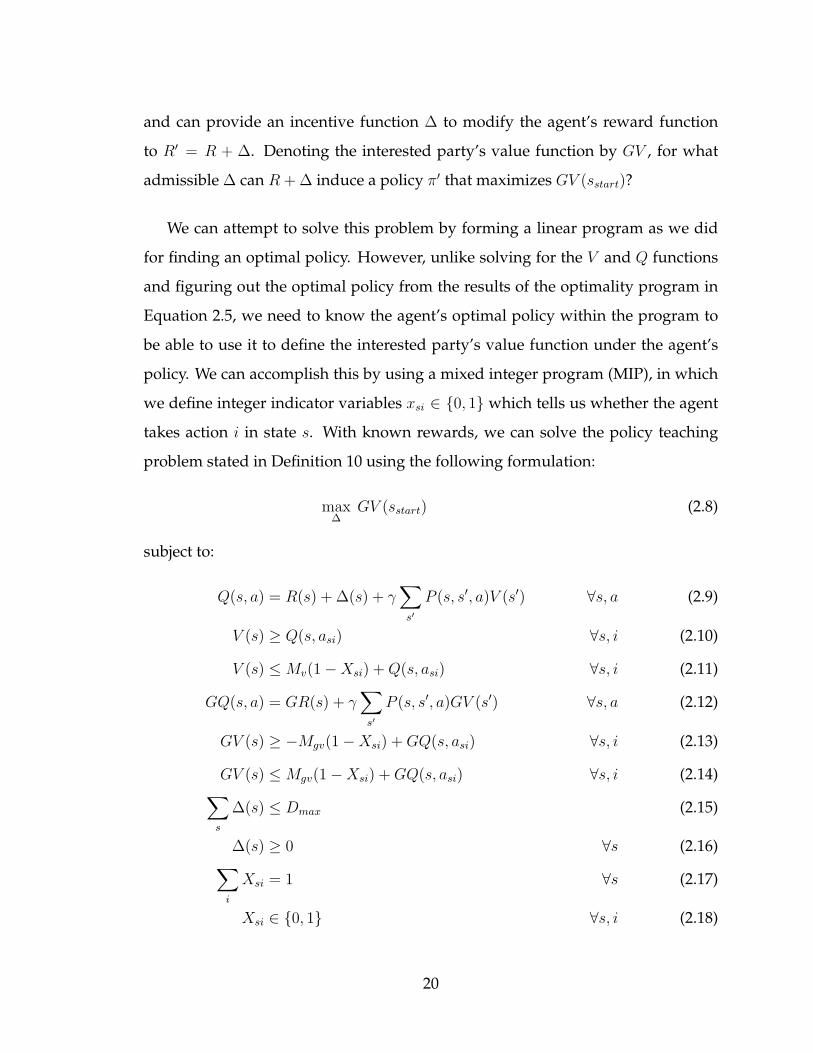
We can attempt to solve this problem by forming a linear program as we did

for finding an optimal policy. However, unlike solving for the V and Q functions

and figuring out the optimal policy from the results of the optimality program in

Equation 2.5, we need to know the agent’s optimal policy within the program to

be able to use it to define the interested party’s value function under the agent’s

policy. We can accomplish this by using a mixed integer program (MIP), in which

we define integer indicator variables xsi ∈ {0, 1} which tells us whether the agent

takes action i in state s. With known rewards, we can solve the policy teaching

problem stated in Definition 10 using the following formulation:

max∆

GV (sstart) (2.8)

subject to:

Q(s, a) = R(s) + ∆(s) + γ∑

s′

P (s, s′, a)V (s′) ∀s, a (2.9)

V (s) ≥ Q(s, asi) ∀s, i (2.10)

V (s) ≤Mv(1−Xsi) + Q(s, asi) ∀s, i (2.11)

GQ(s, a) = GR(s) + γ∑

s′

P (s, s′, a)GV (s′) ∀s, a (2.12)

GV (s) ≥ −Mgv(1−Xsi) + GQ(s, asi) ∀s, i (2.13)

GV (s) ≤Mgv(1−Xsi) + GQ(s, asi) ∀s, i (2.14)∑s

∆(s) ≤ Dmax (2.15)

∆(s) ≥ 0 ∀s (2.16)∑i

Xsi = 1 ∀s (2.17)

Xsi ∈ {0, 1} ∀s, i (2.18)

20

Constants Mv = Mv + |Mv| and Mgv = Mgv + |Mgv| are set such that Mv =

(maxs R(s) + Dmax)/(1 − γ), Mv = mins R(s)/(1 − γ), Mgv = maxs GR(s)/(1 − γ),

and Mv = mins GR(s)/(1 − γ). Constraint 2.9 defines the agent’s Q functions in

terms of R and ∆. Constraints 2.10 and 2.11 ensure that the agent takes the action

with the highest Q value in each state. To see this, consider the two possible values

for Xsi. If Xsi = 1, V (s) = Q(s, asi). By Constraint 2.10, Q(s, asi) = maxi Q(s, i). If

Xsi = 0, the constraints are satisfied because Mv ≥ max V (s)−Q(s, asi).6 Constraint

2.12 defines the interested party’s Q function GQ in terms of GR. Constraints 2.13

and 2.14 ensure that the interested party’s value in a state is equal to the Q value

of the action from the agent’s policy. Constraints 2.15 and 2.16 ensure that ∆ is

admissible, and Constraints 2.17 and 2.18 ensure that exactly one action is chosen

for each state. The objective maximizes the interested party’s value in the start

state.

While the program presented above solves the policy teaching problem stated

in Definition 10, the formulation requires the solution to a mixed integer linear

program, which is an NP-hard problem. Whether the policy teaching problem in

Definition 10 is NP-hard is an open question. Furthermore, while mixed integer

programs can sometimes be solved efficiently, using big-M constants increases the

size of the search space and makes solving MIPs more computationally expensive.

In our formulation, we have chosen the values of Mv and Mgv tightly in an attempt

to control the size of the search space.7 Nevertheless, finding better formulations or

using other approaches for solving the policy teaching problem may be necessary

for some settings.

6Since Mv is the sum of discounted rewards for staying in the state with the highest possiblereward, and Mv is the sum of discounted rewards for staying in the state with the lowest possiblereward, it must be that Mv ≥ max V (s) and Mv ≤ minQ(s, asi). This implies that Mv ≥ max V (s)−Q(s, asi).

7Slightly tighter bounds are possible by defining big-M constants for each state. However, fur-ther tightening will require finding the maximal value achievable in a state given ∆, which is itselfa computationally expensive process (that can be solved by a mixed integer program similar toProgram 2.8).

21

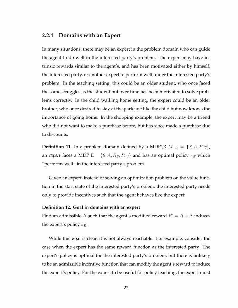
2.2.4 Domains with an Expert

In many situations, there may be an expert in the problem domain who can guide

the agent to do well in the interested party’s problem. The expert may have in-

trinsic rewards similar to the agent’s, and has been motivated either by himself,

the interested party, or another expert to perform well under the interested party’s

problem. In the teaching setting, this could be an older student, who once faced

the same struggles as the student but over time has been motivated to solve prob-

lems correctly. In the child walking home setting, the expert could be an older

brother, who once desired to stay at the park just like the child but now knows the

importance of going home. In the shopping example, the expert may be a friend

who did not want to make a purchase before, but has since made a purchase due

to discounts.

Definition 11. In a problem domain defined by a MDP\R M−R = {S, A, P, γ},

an expert faces a MDP E = {S, A,RE, P, γ} and has an optimal policy πE which

“performs well” in the interested party’s problem.

Given an expert, instead of solving an optimization problem on the value func-

tion in the start state of the interested party’s problem, the interested party needs

only to provide incentives such that the agent behaves like the expert:

Definition 12. Goal in domains with an expert

Find an admissible ∆ such that the agent’s modified reward R′ = R + ∆ induces

the expert’s policy πE .

While this goal is clear, it is not always reachable. For example, consider the

case when the expert has the same reward function as the interested party. The

expert’s policy is optimal for the interested party’s problem, but there is unlikely

to be an admissible incentive function that can modify the agent’s reward to induce

the expert’s policy. For the expert to be useful for policy teaching, the expert must

22

both perform well in the interested party’s problem (i.e. have a high value in the

start state) and perform a policy reachable by the agent given the constraints on ∆.

We can think of the expert as having faced a similar reward as the student and

has since been motivated to perform well in the interested party’s domain. We can

view the expert’s reward RE = RO +∆E as the sum of the expert’s intrinsic reward

RO and the motivation ∆E that he received. Given that RO is similar to the agent’s

reward and ∆E is within the constraints on incentives, we can think of the expert

as having solved a similar policy teaching problem.

Now that we have defined the goal and have discussed the conditions for the

goal to be reachable, we can define the policy teaching problem for domains with

an expert:

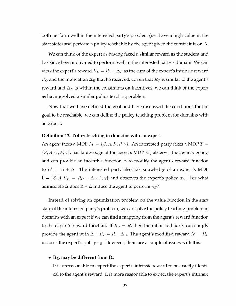
Definition 13. Policy teaching in domains with an expert

An agent faces a MDP M = {S, A,R, P, γ}. An interested party faces a MDP T =

{S, A,G, P, γ}, has knowledge of the agent’s MDP M , observes the agent’s policy,

and can provide an incentive function ∆ to modify the agent’s reward function

to R′ = R + ∆. The interested party also has knowledge of an expert’s MDP

E = {S, A,RE = RO + ∆E, P, γ} and observes the expert’s policy πE . For what

admissible ∆ does R + ∆ induce the agent to perform πE?

Instead of solving an optimization problem on the value function in the start

state of the interested party’s problem, we can solve the policy teaching problem in

domains with an expert if we can find a mapping from the agent’s reward function

to the expert’s reward function. If RO = R, then the interested party can simply

provide the agent with ∆ = RE − R = ∆E . The agent’s modified reward R′ = RE

induces the expert’s policy πE . However, there are a couple of issues with this:

• RO may be different from R.

It is unreasonable to expect the expert’s intrinsic reward to be exactly identi-

cal to the agent’s reward. It is more reasonable to expect the expert’s intrinsic

23

reward to be similar to the agent’s current reward.

• The expert may have used more motivation than necessary to achieve πE.

There may be smaller incentives that the interested party can provide to in-

duce πE than the motivation the expert had used. The expert could have

arrived at his current state through a lot of internal and external motivation,

and it may be unnecessarily costly to provide the same to the agent.

We make two simple observations to deal with these issues. One observation

is that we do not really care whether RO = R, but instead care about whether the

expert’s motivated reward RE is one that the agent can reach given the constraints

on ∆. In other words, if there exists a ∆ = RE−R that is admissible, the interested

party can provide this ∆ such that the agent performs πE . The second observation

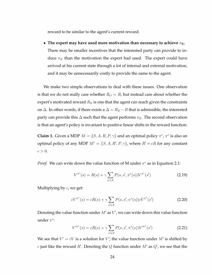
is that an agent’s policy is invariant to positive linear shifts in the reward function:

Claim 1. Given a MDP M = {S, A,R, P, γ} and an optimal policy π∗, π∗ is also an

optimal policy of any MDP M ′ = {S, A,R′, P, γ}, where R′ = cR for any constant

c > 0.

Proof. We can write down the value function of M under π∗ as in Equation 2.1:

V π∗(s) = R(s) + γ

∑s′∈S

P (s, s′, π∗(s))V π∗(s′) (2.19)

Multiplying by c, we get:

cV π∗(s) = cR(s) + γ

∑s′∈S

P (s, s′, π∗(s))cV π∗(s′) (2.20)

Denoting the value function under M ′ as V ′, we can write down this value function

under π∗:

V ′π∗(s) = cR(s) + γ

∑s′∈S

P (s, s′, π∗(s))V ′π∗(s′) (2.21)

We see that V ′ = cV is a solution for V ′; the value function under M ′ is shifted by

c just like the reward R′. Denoting the Q function under M ′ as Q′, we see that the

24

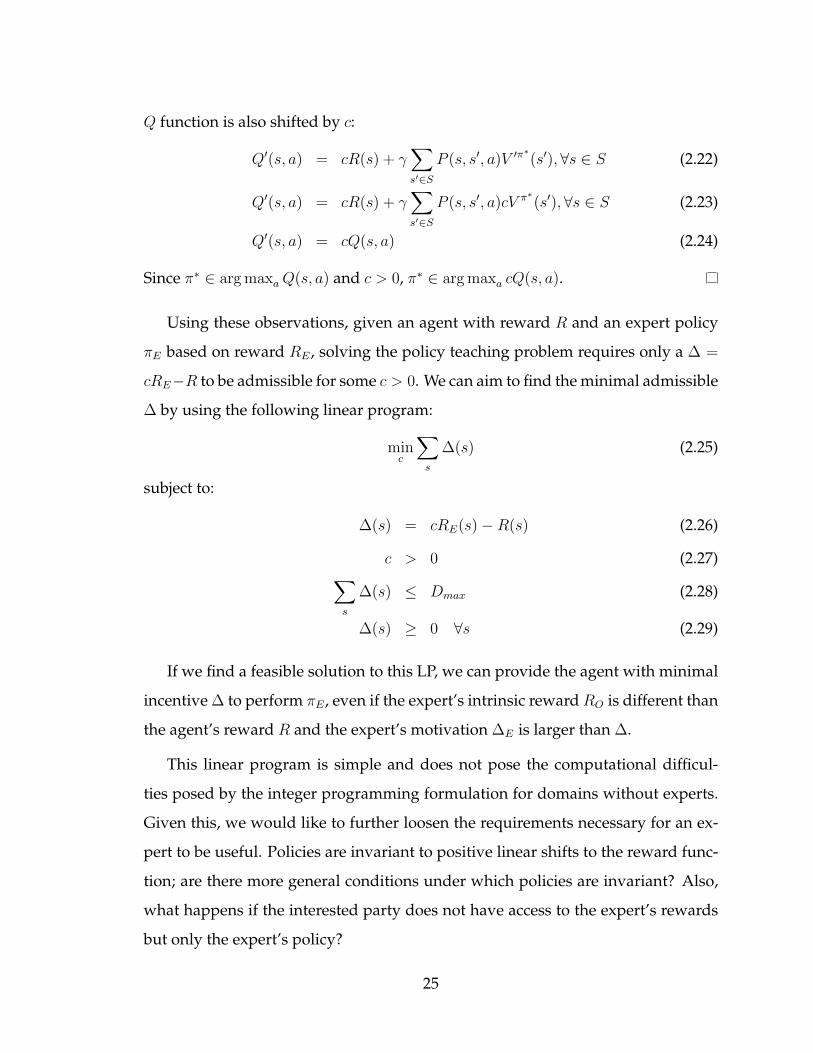
Q function is also shifted by c:

Q′(s, a) = cR(s) + γ∑s′∈S

P (s, s′, a)V ′π∗(s′),∀s ∈ S (2.22)

Q′(s, a) = cR(s) + γ∑s′∈S

P (s, s′, a)cV π∗(s′),∀s ∈ S (2.23)

Q′(s, a) = cQ(s, a) (2.24)

Since π∗ ∈ arg maxa Q(s, a) and c > 0, π∗ ∈ arg maxa cQ(s, a).

Using these observations, given an agent with reward R and an expert policy

πE based on reward RE , solving the policy teaching problem requires only a ∆ =

cRE−R to be admissible for some c > 0. We can aim to find the minimal admissible

∆ by using the following linear program:

minc

∑s

∆(s) (2.25)

subject to:

∆(s) = cRE(s)−R(s) (2.26)

c > 0 (2.27)∑s

∆(s) ≤ Dmax (2.28)

∆(s) ≥ 0 ∀s (2.29)

If we find a feasible solution to this LP, we can provide the agent with minimal

incentive ∆ to perform πE , even if the expert’s intrinsic reward RO is different than

the agent’s reward R and the expert’s motivation ∆E is larger than ∆.

This linear program is simple and does not pose the computational difficul-

ties posed by the integer programming formulation for domains without experts.

Given this, we would like to further loosen the requirements necessary for an ex-

pert to be useful. Policies are invariant to positive linear shifts to the reward func-

tion; are there more general conditions under which policies are invariant? Also,

what happens if the interested party does not have access to the expert’s rewards

but only the expert’s policy?

25

Chapter 3

Policy Teaching with UnknownRewards

In this chapter we introduce inverse reinforcement learning (IRL) as a method for

inferring the space of reward functions that corresponds to a policy, and use the

IRL method to discuss the policy teaching problem with unknown rewards.

3.1 Inverse Reinforcement Learning

As we saw at the end of Chapter 2, better understanding of the space of rewards

that induce a certain policy is useful for policy teaching. First, knowing the space

of rewards that induces the expert’s policy increases the likelihood of having an

admissible incentive function that would induce the agent to perform the expert’s

policy. At the same time, it also allows for the providing of minimal incentives to

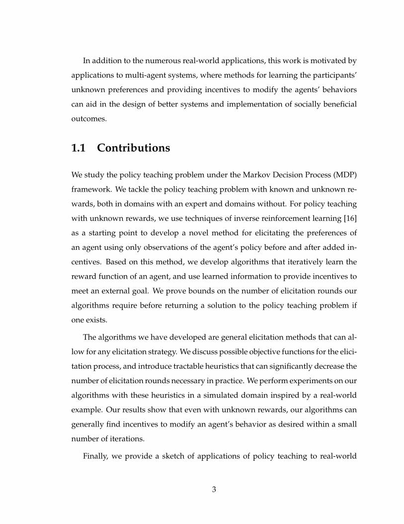
accomplish the same task. To visualize this, we can think of the policy teaching

problem as finding an admissible mapping from the agent’s reward (a point) into

any point in the space of rewards that induce the expert’s policy. Figure 3.1 gives

a pictorial depiction of this operation.

Second, the interested party may only observe the expert’s policy and not the

expert’s reward function. For example, a teacher can see how an excellent student

goes about solving a problem, but have no idea what the student’s reward function

26

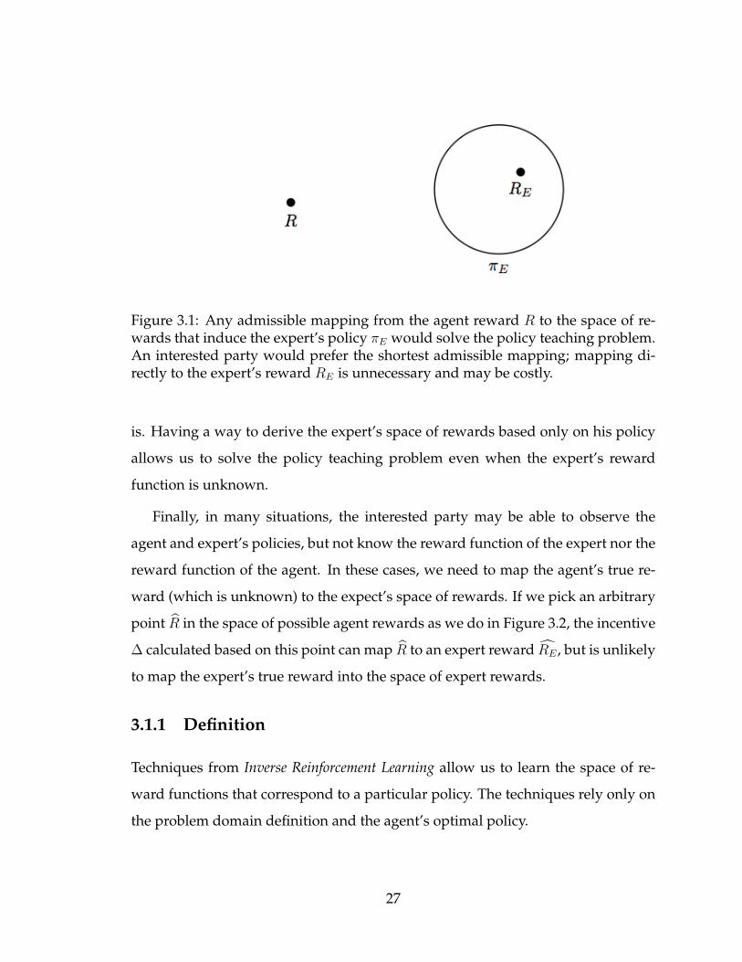
Figure 3.1: Any admissible mapping from the agent reward R to the space of re-wards that induce the expert’s policy πE would solve the policy teaching problem.An interested party would prefer the shortest admissible mapping; mapping di-rectly to the expert’s reward RE is unnecessary and may be costly.

is. Having a way to derive the expert’s space of rewards based only on his policy

allows us to solve the policy teaching problem even when the expert’s reward

function is unknown.

Finally, in many situations, the interested party may be able to observe the

agent and expert’s policies, but not know the reward function of the expert nor the

reward function of the agent. In these cases, we need to map the agent’s true re-

ward (which is unknown) to the expect’s space of rewards. If we pick an arbitrary

point R in the space of possible agent rewards as we do in Figure 3.2, the incentive

∆ calculated based on this point can map R to an expert reward RE , but is unlikely

to map the expert’s true reward into the space of expert rewards.

3.1.1 Definition

Techniques from Inverse Reinforcement Learning allow us to learn the space of re-

ward functions that correspond to a particular policy. The techniques rely only on

the problem domain definition and the agent’s optimal policy.

27

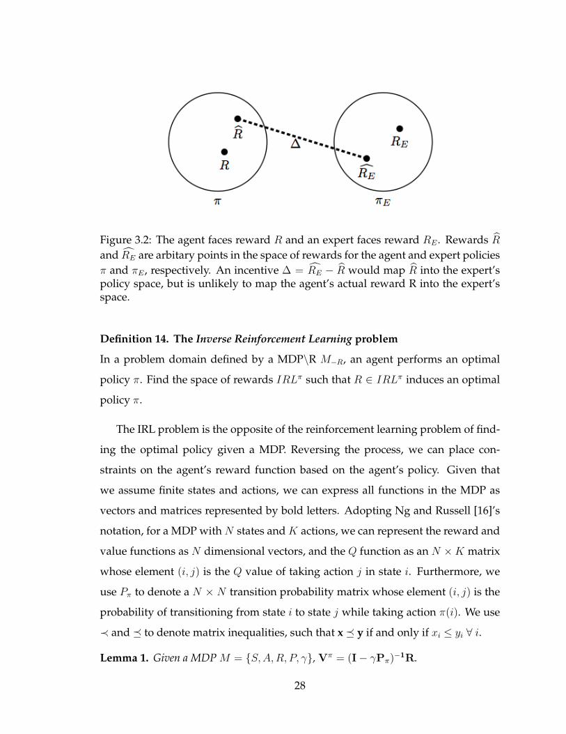
Figure 3.2: The agent faces reward R and an expert faces reward RE . Rewards R

and RE are arbitary points in the space of rewards for the agent and expert policiesπ and πE , respectively. An incentive ∆ = RE − R would map R into the expert’spolicy space, but is unlikely to map the agent’s actual reward R into the expert’sspace.

Definition 14. The Inverse Reinforcement Learning problem

In a problem domain defined by a MDP\R M−R, an agent performs an optimal

policy π. Find the space of rewards IRLπ such that R ∈ IRLπ induces an optimal

policy π.

The IRL problem is the opposite of the reinforcement learning problem of find-

ing the optimal policy given a MDP. Reversing the process, we can place con-

straints on the agent’s reward function based on the agent’s policy. Given that

we assume finite states and actions, we can express all functions in the MDP as

vectors and matrices represented by bold letters. Adopting Ng and Russell [16]’s

notation, for a MDP with N states and K actions, we can represent the reward and

value functions as N dimensional vectors, and the Q function as an N ×K matrix

whose element (i, j) is the Q value of taking action j in state i. Furthermore, we

use Pπ to denote a N × N transition probability matrix whose element (i, j) is the

probability of transitioning from state i to state j while taking action π(i). We use

≺ and � to denote matrix inequalities, such that x � y if and only if xi ≤ yi ∀ i.

Lemma 1. Given a MDP M = {S, A,R, P, γ}, Vπ = (I− γPπ)−1R.

28

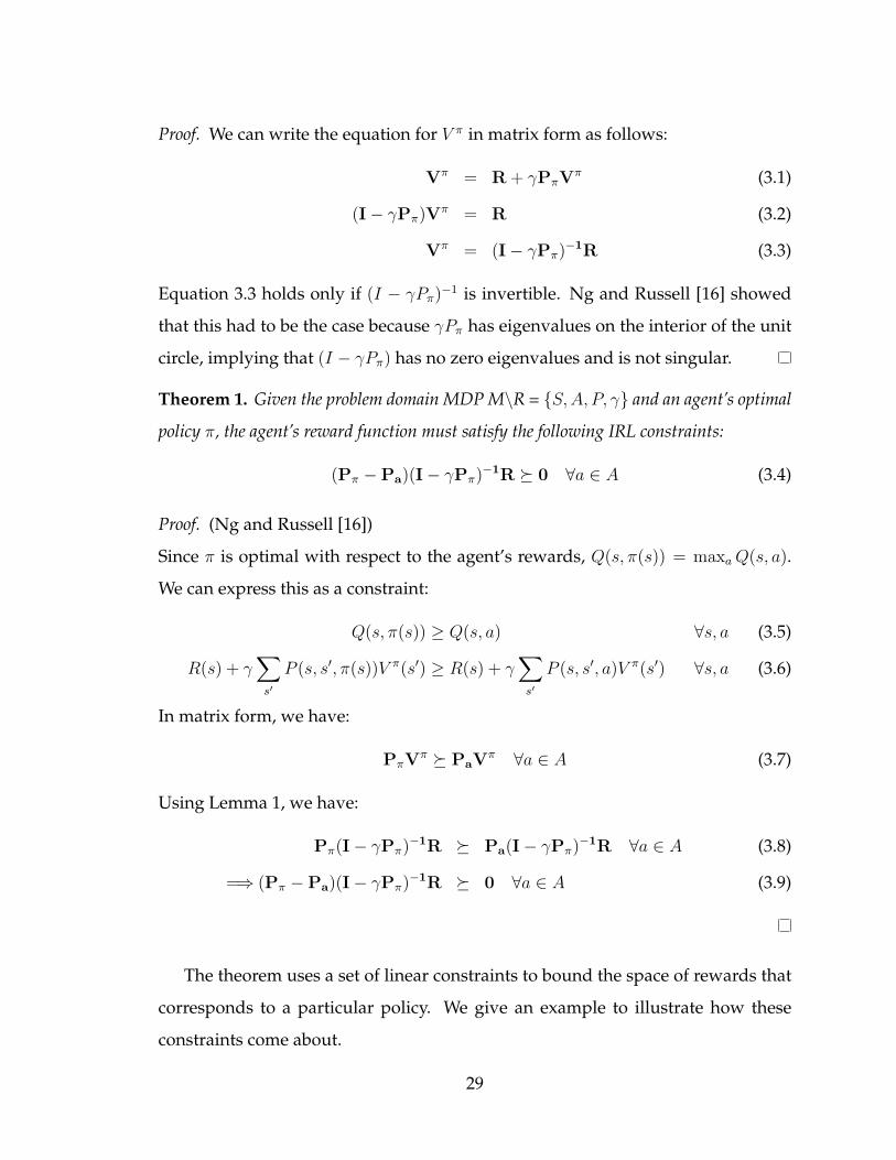
Proof. We can write the equation for V π in matrix form as follows:

Vπ = R + γPπVπ (3.1)

(I− γPπ)Vπ = R (3.2)

Vπ = (I− γPπ)−1R (3.3)

Equation 3.3 holds only if (I − γPπ)−1 is invertible. Ng and Russell [16] showed

that this had to be the case because γPπ has eigenvalues on the interior of the unit

circle, implying that (I − γPπ) has no zero eigenvalues and is not singular.

Theorem 1. Given the problem domain MDP M\R = {S, A, P, γ} and an agent’s optimal

policy π, the agent’s reward function must satisfy the following IRL constraints:

(Pπ −Pa)(I− γPπ)−1R � 0 ∀a ∈ A (3.4)

Proof. (Ng and Russell [16])

Since π is optimal with respect to the agent’s rewards, Q(s, π(s)) = maxa Q(s, a).

We can express this as a constraint:

Q(s, π(s)) ≥ Q(s, a) ∀s, a (3.5)

R(s) + γ∑

s′

P (s, s′, π(s))V π(s′) ≥ R(s) + γ∑

s′

P (s, s′, a)V π(s′) ∀s, a (3.6)

In matrix form, we have:

PπVπ � PaV

π ∀a ∈ A (3.7)

Using Lemma 1, we have:

Pπ(I− γPπ)−1R � Pa(I− γPπ)−1R ∀a ∈ A (3.8)

=⇒ (Pπ −Pa)(I− γPπ)−1R � 0 ∀a ∈ A (3.9)

The theorem uses a set of linear constraints to bound the space of rewards that

corresponds to a particular policy. We give an example to illustrate how these

constraints come about.

29

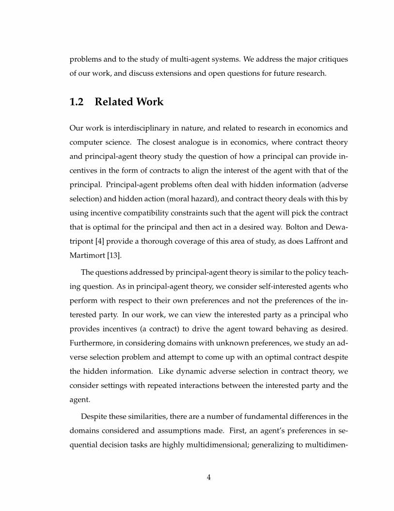
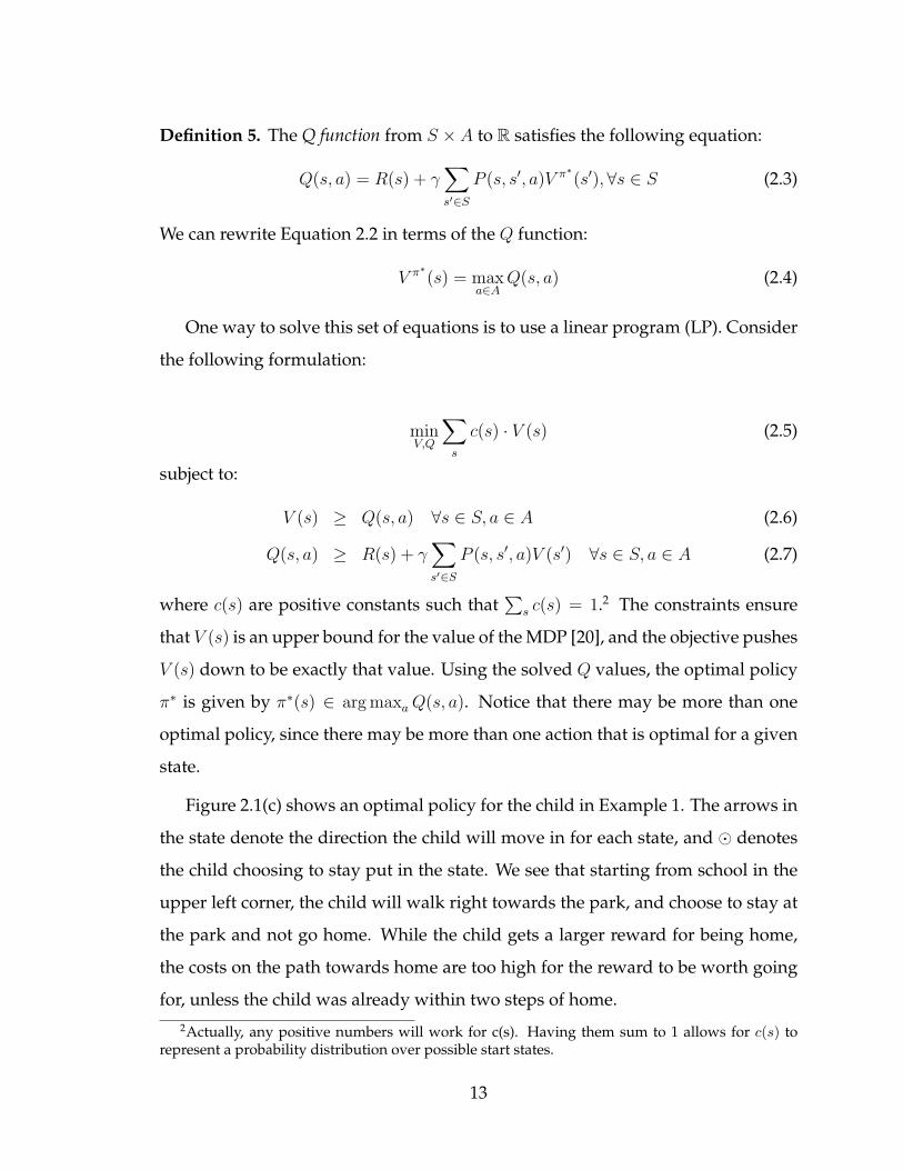
h r r r p(a) state space

� ← ← → �(b) optimal policy

3 0 0 0 3(c) possible reward func-tion

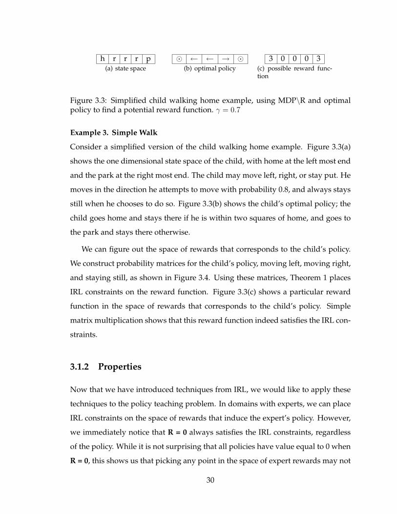
Figure 3.3: Simplified child walking home example, using MDP\R and optimalpolicy to find a potential reward function. γ = 0.7

Example 3. Simple Walk

Consider a simplified version of the child walking home example. Figure 3.3(a)

shows the one dimensional state space of the child, with home at the left most end

and the park at the right most end. The child may move left, right, or stay put. He

moves in the direction he attempts to move with probability 0.8, and always stays

still when he chooses to do so. Figure 3.3(b) shows the child’s optimal policy; the

child goes home and stays there if he is within two squares of home, and goes to

the park and stays there otherwise.

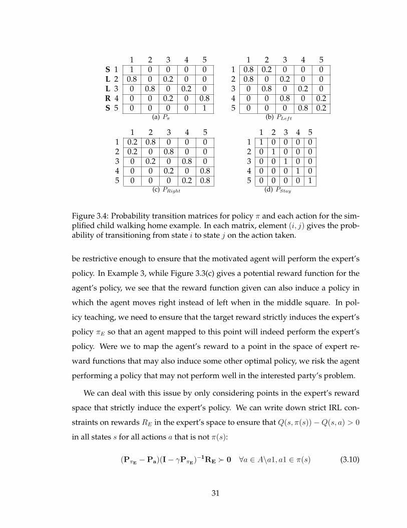
We can figure out the space of rewards that corresponds to the child’s policy.

We construct probability matrices for the child’s policy, moving left, moving right,

and staying still, as shown in Figure 3.4. Using these matrices, Theorem 1 places

IRL constraints on the reward function. Figure 3.3(c) shows a particular reward

function in the space of rewards that corresponds to the child’s policy. Simple

matrix multiplication shows that this reward function indeed satisfies the IRL con-

straints.

3.1.2 Properties

Now that we have introduced techniques from IRL, we would like to apply these

techniques to the policy teaching problem. In domains with experts, we can place

IRL constraints on the space of rewards that induce the expert’s policy. However,

we immediately notice that R = 0 always satisfies the IRL constraints, regardless

of the policy. While it is not surprising that all policies have value equal to 0 when

R = 0, this shows us that picking any point in the space of expert rewards may not

30

1 2 3 4 5S 1 1 0 0 0 0L 2 0.8 0 0.2 0 0L 3 0 0.8 0 0.2 0R 4 0 0 0.2 0 0.8S 5 0 0 0 0 1

(a) Pπ

1 2 3 4 51 0.8 0.2 0 0 02 0.8 0 0.2 0 03 0 0.8 0 0.2 04 0 0 0.8 0 0.25 0 0 0 0.8 0.2

(b) PLeft

1 2 3 4 51 0.2 0.8 0 0 02 0.2 0 0.8 0 03 0 0.2 0 0.8 04 0 0 0.2 0 0.85 0 0 0 0.2 0.8

(c) PRight

1 2 3 4 51 1 0 0 0 02 0 1 0 0 03 0 0 1 0 04 0 0 0 1 05 0 0 0 0 1

(d) PStay

Figure 3.4: Probability transition matrices for policy π and each action for the sim-plified child walking home example. In each matrix, element (i, j) gives the prob-ability of transitioning from state i to state j on the action taken.

be restrictive enough to ensure that the motivated agent will perform the expert’s

policy. In Example 3, while Figure 3.3(c) gives a potential reward function for the

agent’s policy, we see that the reward function given can also induce a policy in

which the agent moves right instead of left when in the middle square. In pol-

icy teaching, we need to ensure that the target reward strictly induces the expert’s

policy πE so that an agent mapped to this point will indeed perform the expert’s

policy. Were we to map the agent’s reward to a point in the space of expert re-

ward functions that may also induce some other optimal policy, we risk the agent

performing a policy that may not perform well in the interested party’s problem.

We can deal with this issue by only considering points in the expert’s reward

space that strictly induce the expert’s policy. We can write down strict IRL con-

straints on rewards RE in the expert’s space to ensure that Q(s, π(s))−Q(s, a) > 0

in all states s for all actions a that is not π(s):

(PπE−Pa)(I− γPπE

)−1RE � 0 ∀a ∈ A\a1, a1 ∈ π(s) (3.10)

31

The use of these strict IRL constraints removes reward functions that induce

more than one optimal policy from consideration, but does not prevent a reward

function to be found. Given an action π(s) from an optimal policy π, the only

cases in which another action a′ must necessarily be as good as a is when the state

transition functions for both actions are identical in state s. In such cases, we can

just model these two actions in the state as the same action.

To use these strict IRL constraints on the expert’s reward in a linear program,

we need to represent the constraint as a non-strict inequality. We can do this by

using a small constant ε > 0, such that the slack between the Q values of the best

and second best action in a state is least ε. We can rewrite the constraint as follows:

(PπE−Pa)(I− γPπE

)−1RE � ε ∀a ∈ A\a1, a1 ∈ π(s) (3.11)

We denote a reward function RE that satisfies this constraint as RE ∈ IRLπEstrict.

Given an expert’s policy πE and the agent’s reward R, we can now solve the policy

teaching problem in domains with experts using the following linear program:

minRE

∑s

∆(s) (3.12)

subject to:

∆(s) = RE(s)−R(s) ∀s ∈ S (3.13)

(PπE−Pa)(I− γPπE

)−1RE � ε ∀a ∈ A\a1, a1 ∈ π(s) (3.14)∑s

∆(s) ≤ Dmax (3.15)

∆(s) ≥ 0 ∀s ∈ S (3.16)

where RE are variables on the target reward in the reward space of the expert’s

policy. The program is still a tractable LP and provides an improvement over

Program 2.25 to capture policy invariance beyond just linear shifts in the reward

function. Furthermore, Program 3.12 does not require knowledge of the expert’s

32

reward function, again loosening the observability requirements on the interested

party.

The use of IRL constraints have allowed us to complete our discussion of policy

teaching with known rewards. However, what happens when we do not know the

agent’s reward? IRL gives the space of rewards that induce the agent’s policy, but

how do we find the agent’s reward out of that space as to be able to map it to the

desired space?

3.2 Policy Teaching with Unknown Rewards

3.2.1 Setup

Definition 15. Policy teaching with unknown rewards

An agent faces a MDP M = {S, A,R, P, γ} and performs an optimal policy π. An

interested party knows the problem definition MDP\R M−R = {S, A, P, γ}, ob-

serves the agent’s policy, but does not know the agent’s reward R. The interested

party wishes for the agent’s policy to perform well under the interested party’s

problem modeled by a similar MDP T = {S, A,G, P, γ}, and can provide an ad-

missible incentive ∆ to modify the agent’s reward function to R′ = R +∆. Can the

interested party learn about the agent’s reward function as to be able to provide

a ∆ for which the agent’s induced optimal policy π′ with respect to the modified

MDP M ′ = {S, A,R′, P, γ} performs well with respect to T ?

This problem is more interesting than policy teaching with known rewards, and

also more difficult. The problem is more interesting because in most situations, the

interested party will not know the reward function of the agent. Even in cases in

which an agent does not mind sharing his preferences with the interested party,

the agent may not be able to articulate his reward function despite being able to

perform optimally with respect to his preferences.

The problem is also much harder than policy teaching with known rewards.

33

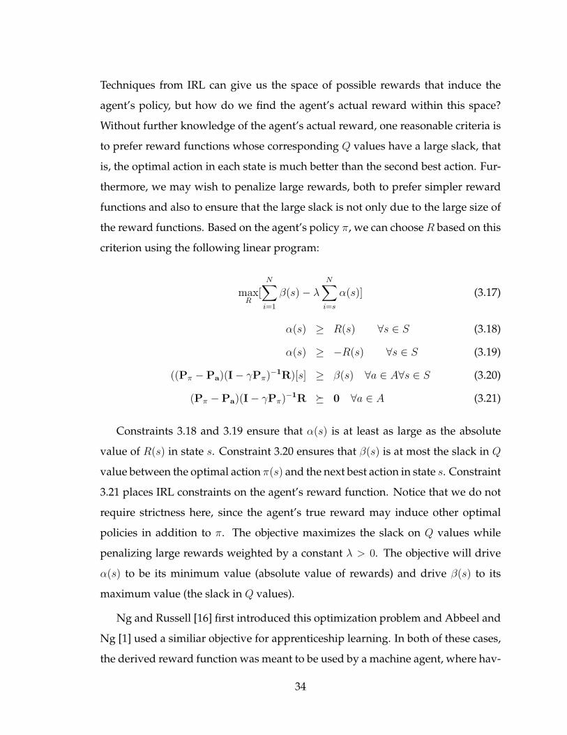
Techniques from IRL can give us the space of possible rewards that induce the

agent’s policy, but how do we find the agent’s actual reward within this space?

Without further knowledge of the agent’s actual reward, one reasonable criteria is

to prefer reward functions whose corresponding Q values have a large slack, that

is, the optimal action in each state is much better than the second best action. Fur-

thermore, we may wish to penalize large rewards, both to prefer simpler reward

functions and also to ensure that the large slack is not only due to the large size of

the reward functions. Based on the agent’s policy π, we can choose R based on this

criterion using the following linear program:

maxR

[N∑

i=1

β(s)− λN∑

i=s

α(s)] (3.17)

α(s) ≥ R(s) ∀s ∈ S (3.18)

α(s) ≥ −R(s) ∀s ∈ S (3.19)

((Pπ −Pa)(I− γPπ)−1R)[s] ≥ β(s) ∀a ∈ A∀s ∈ S (3.20)

(Pπ −Pa)(I− γPπ)−1R � 0 ∀a ∈ A (3.21)

Constraints 3.18 and 3.19 ensure that α(s) is at least as large as the absolute

value of R(s) in state s. Constraint 3.20 ensures that β(s) is at most the slack in Q

value between the optimal action π(s) and the next best action in state s. Constraint

3.21 places IRL constraints on the agent’s reward function. Notice that we do not

require strictness here, since the agent’s true reward may induce other optimal

policies in addition to π. The objective maximizes the slack on Q values while

penalizing large rewards weighted by a constant λ > 0. The objective will drive

α(s) to be its minimum value (absolute value of rewards) and drive β(s) to its

maximum value (the slack in Q values).

Ng and Russell [16] first introduced this optimization problem and Abbeel and

Ng [1] used a similiar objective for apprenticeship learning. In both of these cases,

the derived reward function was meant to be used by a machine agent, where hav-

34

ing large slack and simple reward functions allow the machine agent to perform

well even with slight changes to the problem domain. In our case, the derived re-

ward function needs to resemble the agent’s true reward, based on which we can

find the incentive function to map the agent’s reward to the reward space of the

expert’s policy. Applied to policy teaching, Program 3.17 gives us a heuristic for

picking a point in the agent’s reward space, but otherwise does little to provide us

more information on the agent’s true reward.

In order to make progress towards learning the agent’s reward function, it is

necessary to be able to narrow the space of possible agent rewards by eliminating

rewards in the space that are not the agent’s actual reward. If we can gain addi-

tional evidence about the agent’s reward, we may be able to use the evidence to

further constrain the space of possible rewards.

3.2.2 Elicitation Method

One way to gain new evidence about the agent’s reward function is for the in-

terested party to perform direct preference elicitation by asking queries about the

agent’s preferences. Queries often considered in the literature [22] include rank

queries (“What is your second-most preferred policy?”), order queries (“Is policy

a preferred to policy b?”), bound queries (“Is your reward in state s at least rs?”),

and value queries (“what is your reward in state s?”). Responses to queries can be

used to introduce additional constraints on the agent’s reward function (in addi-

tion to IRL constraints), which in turn narrows the space of rewards.

While direct preference elicitation have been used successfully in many set-

tings, there are a number of issues that suggest that direct querying may be infea-

sible in the sequential decision making domains we consider:

• Interconnected states.

The quality of an action in a state is dependent on the rewards and actions

in other states. Asking queries on the reward in a certain state requires the

35

agent to place explicit weights on individual states and consider a state in

isolation of other states and actions. While reward functions are succinct

representations of agent preferences in MDPs, it is not clear that an agent

can express his preferences in this way given the interdependencies between

different states and actions.

• Policy-based queries are hard to answer.

While order queries comparing the optimal policy to any other policy are

trivial to answer, it is not clear that rank and order queries on non-optimal

policies are easy to answer. In a setting with N states and K actions, there are

KN possible stationary policies, most of which the agent probably has never

considered explicitly.

• Nonmonetary rewards are hard to articulate.

In many of the examples that we are interested in, the agent’s preferences

are nonmonetary. Furthermore, the incentives provided may also be non-

monetary, and could be of a different denomination than the agent’s internal

preferences. For bound and value queries, the agent would need to be able to

express his preferences in the same denomination as the incentives provided.

• Getting the agent to answer queries may be difficult.

In monetary situations such as auctions, getting an agent to participate in an

elicitation process is “simple” - the agent must participate in order to par-

ticipate in the auction. In policy teaching problems, it is not clear how the

interested party can get the agent to answer queries.

Due to these issues, we consider instead methods of indirect elicitation, that is,

using observations of an agent’s behavior to make inferences about his preferences.

With IRL, we are already doing indirect elicitation by using the agent’s policy to

find the space of reward functions that correspond to that policy. With one policy,

however, we only have one set of IRL constraints. How can we generate more

36

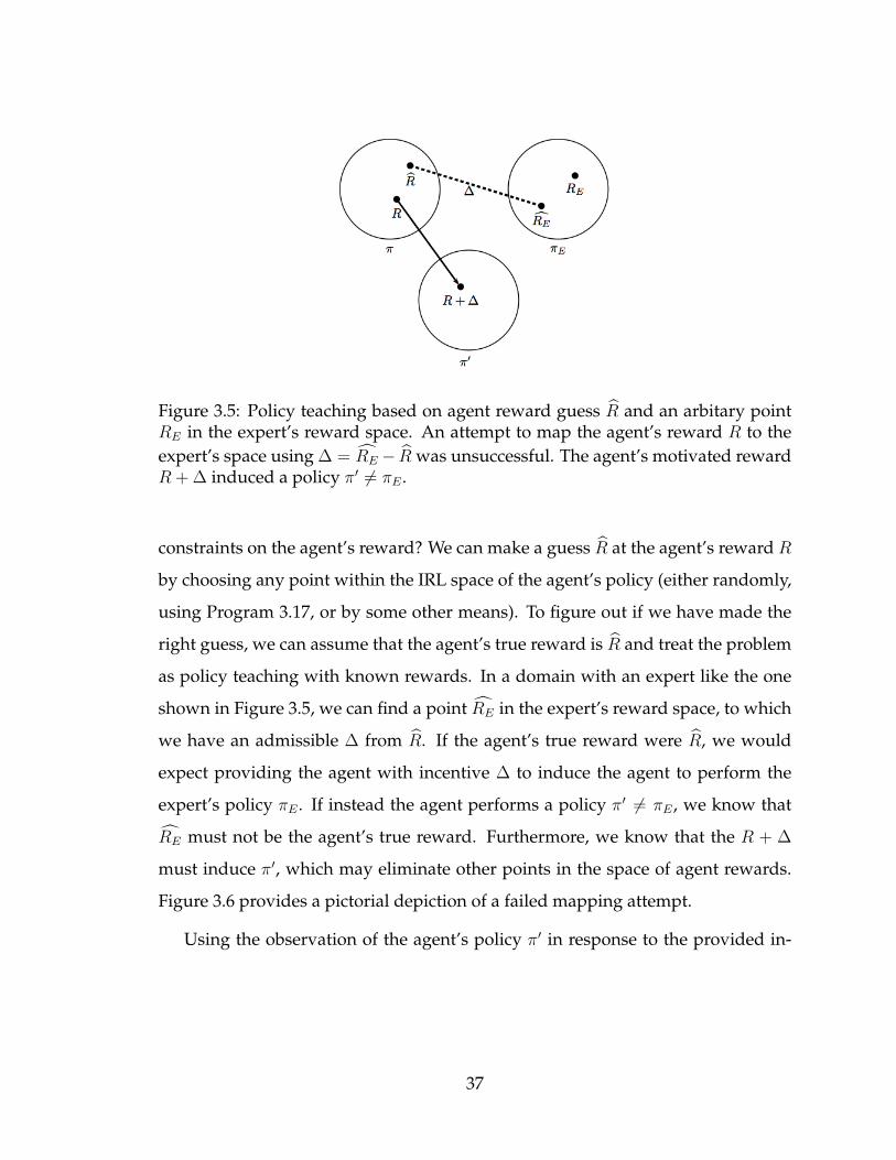
Figure 3.5: Policy teaching based on agent reward guess R and an arbitary pointRE in the expert’s reward space. An attempt to map the agent’s reward R to theexpert’s space using ∆ = RE − R was unsuccessful. The agent’s motivated rewardR + ∆ induced a policy π′ 6= πE .

constraints on the agent’s reward? We can make a guess R at the agent’s reward R

by choosing any point within the IRL space of the agent’s policy (either randomly,

using Program 3.17, or by some other means). To figure out if we have made the

right guess, we can assume that the agent’s true reward is R and treat the problem

as policy teaching with known rewards. In a domain with an expert like the one

shown in Figure 3.5, we can find a point RE in the expert’s reward space, to which

we have an admissible ∆ from R. If the agent’s true reward were R, we would

expect providing the agent with incentive ∆ to induce the agent to perform the

expert’s policy πE . If instead the agent performs a policy π′ 6= πE , we know that

RE must not be the agent’s true reward. Furthermore, we know that the R + ∆

must induce π′, which may eliminate other points in the space of agent rewards.

Figure 3.6 provides a pictorial depiction of a failed mapping attempt.

Using the observation of the agent’s policy π′ in response to the provided in-

37

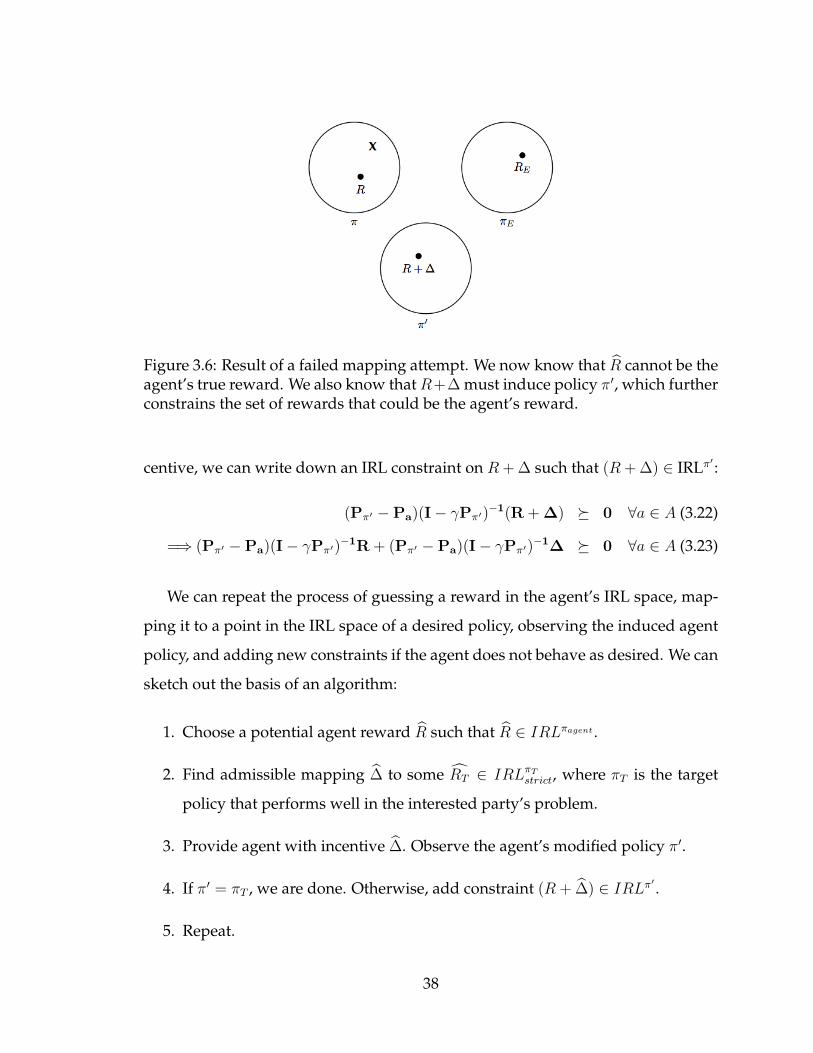
Figure 3.6: Result of a failed mapping attempt. We now know that R cannot be theagent’s true reward. We also know that R+∆ must induce policy π′, which furtherconstrains the set of rewards that could be the agent’s reward.

centive, we can write down an IRL constraint on R + ∆ such that (R + ∆) ∈ IRLπ′ :

(Pπ′ −Pa)(I− γPπ′)−1(R + ∆) � 0 ∀a ∈ A (3.22)

=⇒ (Pπ′ −Pa)(I− γPπ′)−1R + (Pπ′ −Pa)(I− γPπ′)−1∆ � 0 ∀a ∈ A (3.23)

We can repeat the process of guessing a reward in the agent’s IRL space, map-

ping it to a point in the IRL space of a desired policy, observing the induced agent

policy, and adding new constraints if the agent does not behave as desired. We can

sketch out the basis of an algorithm:

1. Choose a potential agent reward R such that R ∈ IRLπagent .

2. Find admissible mapping ∆ to some RT ∈ IRLπTstrict, where πT is the target

policy that performs well in the interested party’s problem.

3. Provide agent with incentive ∆. Observe the agent’s modified policy π′.

4. If π′ = πT , we are done. Otherwise, add constraint (R + ∆) ∈ IRLπ′ .

5. Repeat.

38

The IRL constraints on the target policy are strict to ensure that the agent per-

forms the desired policy when we have the right guess R for R. Note that we learn

about the agent’s reward only for the purpose of finding an admissible mapping to

the IRL space of the target policy. This suggests that it is possible to find a mapping

to the desired policy before we have found the agent’s exact reward R..

This algorithm sketch gives us a general way of thinking about policy teaching

with unknown rewards, which we use to construct algorithms for policy teaching

in domains with and without an expert.

3.2.3 Domains with an Expert

Definition 16. Policy teaching with unknown rewards in domains with an expert

An agent faces a MDP M = {S, A,R, P, γ} and performs the optimal policy π. An

interested party knows the problem definition MDP\R M−R = {S, A, P, γ} and

observes the agent’s policy, but does not know the agent’s reward R. The interested

party also observes an expert’s policy πE , but does not know the expert’s reward

RE . The interested party may provide an admissible incentive ∆ to modify the

agent’s reward function to R′ = R + ∆. Can the interested party learn about the

agent’s reward function so as to be able to provide a ∆ such that the agent performs

the expert policy πE?

The expert’s policy offers a clear target IRL space into which we can attempt to

map the reward of the agent. In guessing a R for the agent’s reward, we can restrict

our attention to rewards in the agent’s IRL space that has admissible mappings into

the expert’s IRL space. We can accomplish this by combining step 2 and 3 of the

algorithm sketch to find R and ∆ simultaneously instead of guessing R and then

seeing if there is an admissible ∆ from R to a point in the expert’s IRL space.

We adopt the following notation for our algorithm. We write IRL constraints

on a reward variable R as R ∈ IRLπ. All constraints are added to a constraint set K,

such that the instantiations of variables must satisfy all constraints in K (but may

39

take on any value as long as it does satisify the constraints in K). An instantiation

of a variable R is denoted as R.

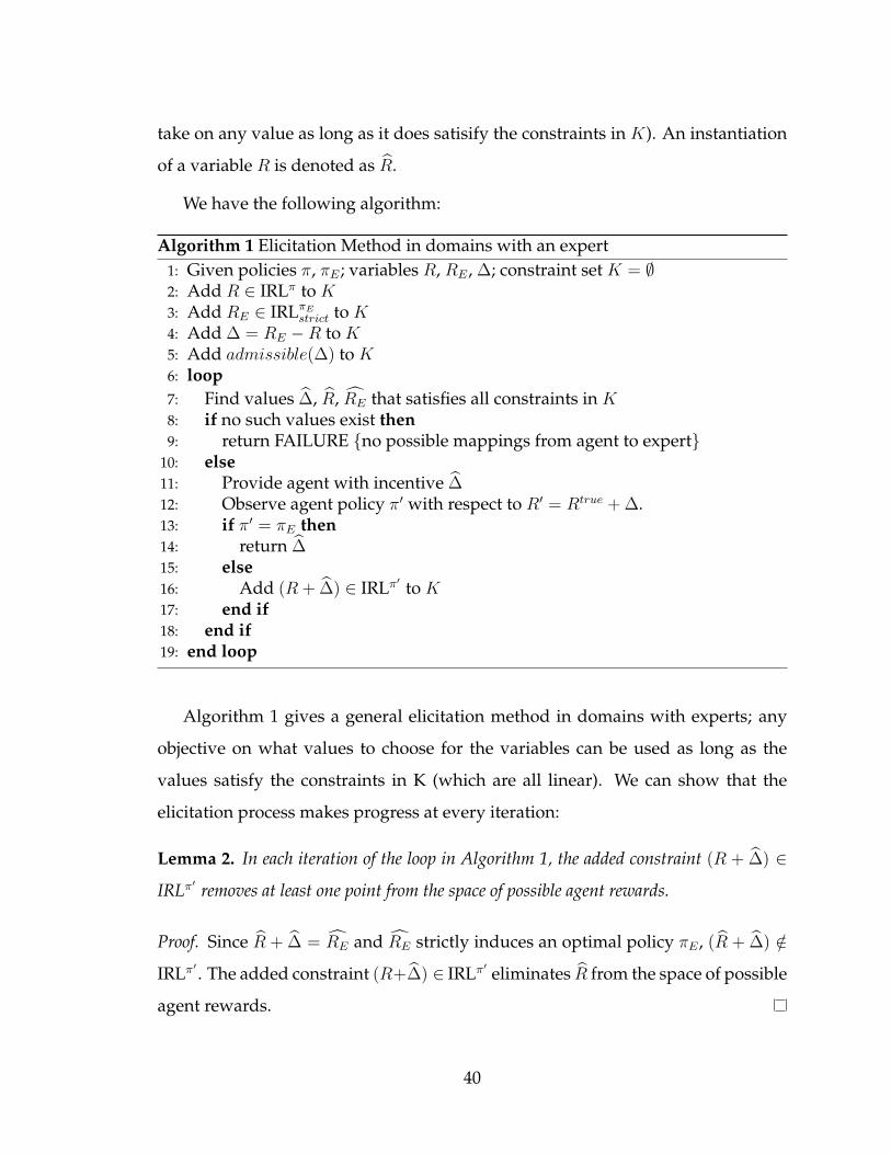
We have the following algorithm:

Algorithm 1 Elicitation Method in domains with an expert1: Given policies π, πE ; variables R, RE , ∆; constraint set K = ∅2: Add R ∈ IRLπ to K3: Add RE ∈ IRLπE

strict to K4: Add ∆ = RE −R to K5: Add admissible(∆) to K6: loop7: Find values ∆, R, RE that satisfies all constraints in K8: if no such values exist then9: return FAILURE {no possible mappings from agent to expert}

10: else11: Provide agent with incentive ∆12: Observe agent policy π′ with respect to R′ = Rtrue + ∆.13: if π′ = πE then14: return ∆15: else16: Add (R + ∆) ∈ IRLπ′ to K17: end if18: end if19: end loop

Algorithm 1 gives a general elicitation method in domains with experts; any

objective on what values to choose for the variables can be used as long as the

values satisfy the constraints in K (which are all linear). We can show that the

elicitation process makes progress at every iteration:

Lemma 2. In each iteration of the loop in Algorithm 1, the added constraint (R + ∆) ∈

IRLπ′ removes at least one point from the space of possible agent rewards.

Proof. Since R + ∆ = RE and RE strictly induces an optimal policy πE , (R + ∆) /∈

IRLπ′ . The added constraint (R+∆) ∈ IRLπ′ eliminates R from the space of possible

agent rewards.

40

Theorem 2. If R(s) is discrete over R for all s, Algorithm 1 terminates in a finite number

of steps with an admissible mapping ∆, or returns FAILURE if no such mapping exists.

Proof. By Assumption 2, R(s) is bounded. If R(s) is also discrete, R(s) must be

finite. Since the state space is finite by Assumption 1, there must only be a finite

number of possible agent reward functions. By Lemma 2, either one of these re-

ward functions is eliminated in each iteration or the elicitation process terminates.

This implies that in a finite number of iterations, the algorithm either finds an ad-

missible mapping or determines that no admissible mapping is possible when all

possible rewards have been eliminated. Since each iteration takes a finite number

of steps, the elicitation process must terminate in a finite number of steps.

When the space of possible agent rewards is discrete (or has been discretized),

Theorem 2 ensures completion of the elicitation process within a finite number of

steps. Generally, we expect the agent’s reward function to arise from a continuous

spectrum; considering a discrete space of possible agent rewards may be too re-

strictive to capture the agent’s true reward. The following lemmas make progress

towards a more general theorem for non-discrete agent rewards:

Lemma 3. Given a MDP M = {S, A,R, T, γ}, we can construct a perturbed MDP M’

= {S, A,R′, T, γ} such that |R′(s) − R(s)| ≤ δ, ∀s ∈ S, δ > 0. Denoting Q as the Q

function for M and Q′ as the Q function for M ′, ∀s ∈ S, a ∈ A:

|Q′(s, a)−Q(s, a)| ≤ δ

1− γ(3.24)

Furthermore, ∀s ∈ S, a, a′ ∈ A, we can bound the change in slack by:

|(Q′(s, a)−Q′(s, a′))− (Q(s, a)−Q(s, a′))| ≤ 2δγ

1− γ(3.25)

Proof. To cause the largest perturbation to the Q value, we must perturb the re-

ward in every state in the same direction. Since the reward function is perturbed

by at most δ in each state, the greatest series of perturbations that can contribute to

41

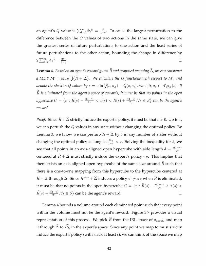
an agent’s Q value is∑∞

k=0 δγk = δ1−γ

. To cause the largest perturbation to the

difference between the Q values of two actions in the same state, we can give

the greatest series of future perturbations to one action and the least series of

future perturbations to the other action, bounding the change in difference by

2∑∞

k=0 δγk = 2δγ1−γ

.

Lemma 4. Based on an agent’s reward guess R and proposed mapping ∆, we can construct

a MDP M’ = M−R

⋃{R + ∆}. We calculate the Q functions with respect to M ′, and

denote the slack in Q values by ε = min Q(s, πE) − Q(s, as), ∀s ∈ S, as ∈ A\πE(s). If

R is eliminated from the agent’s space of rewards, it must be that no points in the open

hypercube C = {x : R(s) − ε(1−γ)2γ

< x(s) < R(s) + ε(1−γ)2γ

,∀s ∈ S} can be the agent’s

reward.

Proof. Since R + ∆ strictly induce the expert’s policy, it must be that ε > 0. Up to ε,

we can perturb the Q values in any state without changing the optimal policy. By

Lemma 3, we know we can perturb R + ∆ by δ in any number of states without

changing the optimal policy as long as 2δγ1−γ

< ε. Solving the inequality for δ, we

see that all points in an axis-aligned open hypercube with side length δ = ε(1−γ)2γ

centered at R + ∆ must strictly induce the expert’s policy πE . This implies that

there exists an axis-aligned open hypercube of the same size around R such that

there is a one-to-one mapping from this hypercube to the hypercube centered at

R + ∆ through ∆. Since Rtrue + ∆ induces a policy π′ 6= πE when R is eliminated,

it must be that no points in the open hypercube C = {x : R(s) − ε(1−γ)2γ

< x(s) <

R(s) + ε(1−γ)2γ

,∀s ∈ S} can be the agent’s reward.

Lemma 4 bounds a volume around each eliminated point such that every point

within the volume must not be the agent’s reward. Figure 3.7 provides a visual

representation of this process. We pick R from the IRL space of πagent, and map

it through ∆ to RE in the expert’s space. Since any point we map to must strictly

induce the expert’s policy (with slack at least ε), we can think of the space we map

42

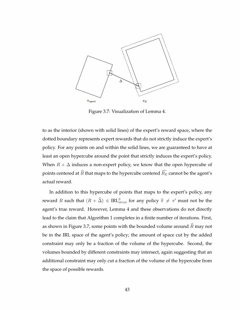
Figure 3.7: Visualization of Lemma 4.

to as the interior (shown with solid lines) of the expert’s reward space, where the

dotted boundary represents expert rewards that do not strictly induce the expert’s

policy. For any points on and within the solid lines, we are guaranteed to have at

least an open hypercube around the point that strictly induces the expert’s policy.

When R + ∆ induces a non-expert policy, we know that the open hypercube of

points centered at R that maps to the hypercube centered RE cannot be the agent’s

actual reward.

In addition to this hypercube of points that maps to the expert’s policy, any

reward R such that (R + ∆) ∈ IRLbπstrict for any policy π 6= π′ must not be the

agent’s true reward. However, Lemma 4 and these observations do not directly

lead to the claim that Algorithm 1 completes in a finite number of iterations. First,

as shown in Figure 3.7, some points with the bounded volume around R may not

be in the IRL space of the agent’s policy; the amount of space cut by the added

constraint may only be a fraction of the volume of the hypercube. Second, the

volumes bounded by different constraints may intersect, again suggesting that an

additional constraint may only cut a fraction of the volume of the hypercube from

the space of possible rewards.

43

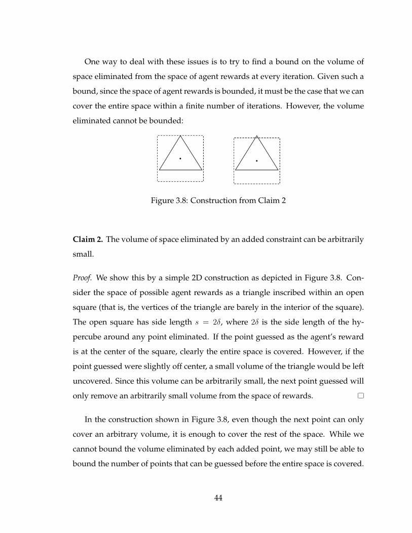
One way to deal with these issues is to try to find a bound on the volume of

space eliminated from the space of agent rewards at every iteration. Given such a

bound, since the space of agent rewards is bounded, it must be the case that we can

cover the entire space within a finite number of iterations. However, the volume

eliminated cannot be bounded:

Figure 3.8: Construction from Claim 2

Claim 2. The volume of space eliminated by an added constraint can be arbitrarily

small.

Proof. We show this by a simple 2D construction as depicted in Figure 3.8. Con-

sider the space of possible agent rewards as a triangle inscribed within an open

square (that is, the vertices of the triangle are barely in the interior of the square).

The open square has side length s = 2δ, where 2δ is the side length of the hy-

percube around any point eliminated. If the point guessed as the agent’s reward

is at the center of the square, clearly the entire space is covered. However, if the

point guessed were slightly off center, a small volume of the triangle would be left

uncovered. Since this volume can be arbitrarily small, the next point guessed will

only remove an arbitrarily small volume from the space of rewards.

In the construction shown in Figure 3.8, even though the next point can only

cover an arbitrary volume, it is enough to cover the rest of the space. While we

cannot bound the volume eliminated by each added point, we may still be able to

bound the number of points that can be guessed before the entire space is covered.

44

By a pigeonhole argument, we show that only a finite number of such points can

fit within the space:

Lemma 5. Given a bounded subspace K in Rn, for some r > 0, we place a set of points

S = {x, y : |xi − yi| > r, 1 ≤ i ≤ n} in K. S must be finite.

Proof. We start by partitioning K into a grid of n-dimensional cubes (see Figure 3.9

for a 2D depiction) each with side length r, such that the farthest distance along

any one dimension between any two points within a cube is r. Since K is bounded,

it must be covered by some finite number m of such cubes. Consider a point being

placed in K; it must fall within one of the cubes. Since there is no other point

within the cube that is more than r away along any dimension, no other points can

be placed within the cube where the point resides. Since each point must take up

at least one cube and there is a finite number of cubes that cover K, only a finite

number of points can be placed in K.

Figure 3.9: Visualization of Lemma 5.

Theorem 3. Algorithm 1 terminates in a finite number of steps with an admissible map-

ping ∆, or returns FAILURE if no such mapping exists.

45

Proof. Every iteration of Algorithm 1 finds R and ∆ that strictly induce the ex-

pert’s policy πE with slack at least ε. By Lemma 4, each R eliminated has an open

hypercube with positive side length 2δ = ε(1−γ)γ

centered at R such that all points

within this hypercube are not the agent’s reward function. Since points in this hy-

percube are not considered in future iterations, no R may be within more than one

hypercube. This implies that any R to be eliminated must be at least δ away from

any other R eliminated. Since R(s) is bounded (by Assumption 2) and the state

space is finite (by Assumption 1), Lemma 5 ensures that only a finite number of

points R may be placed in the space of agent rewards such that each point is more

than (1 − κ)δ away from another, for some small κ > 0. This implies that only a

finite number of guesses R need to be eliminated in order to cover the entire space

of possible agent rewards. Algorithm 1 will terminate in a finite number of steps

either by finding an admissible mapping ∆ before the entire space is covered, or

returning FAILURE once the space is all covered.

This proof makes use of the minimal slack ε that is guaranteed when choosing

a reward function in the IRL space of the expert’s policy. To visualize this, we can

think of the expert’s reward space that is being mapped to as having a border with

a width of δ as shown in Figure 3.7. As such, every mapped-to point has an open

hypercube around it such that all points in this open hypercube still induce the ex-

pert’s policy. This implies that there is an open hypercube of the same size around a

possible agent reward R, such that through ∆, there is a one-to-one mapping from

each of these points to the points in the hypercube around the expert’s reward,

points that all strictly induce the expert’s policy. As such, these points violate the

constraint that (R + ∆) ∈ IRLπ′ and are removed from consideration. Figure 3.9

shows that each point removed this way must completely cover at least one new

square (shown in light gray) from the grid of squares that covers the agent’s re-

ward space, even though the spaces covered by the squares may intersect or be

outside the space of agent rewards. This ensures that we can cover the space in a

46

finite number of iterations.

The number of iterations necessary to complete the elicitation process is de-

pendent on the minimal slack ε and the discount factor γ. Increasing the slack

decreases the number of potential iterations required to cover the entire space.

Generally, as long as ε is set to be much smaller than the limits on the incentives

provided, it is virtually impossible for ε to prevent an admissible mapping to the

expert’s reward space that would have otherwise existed were ε any smaller.

3.2.4 Domains without an Expert

We have provided a general elicitation algorithm for policy teaching in domains

with an expert. In trying to come up with an elicitation algorithm for domains

without an expert, we are confronted with a couple of new issues. First, in do-

mains with an expert, there is the expert’s policy to map to such that the elicitation

process completes as soon as we hit any points in the reward space of that policy.

In domains without an expert, we do not have a specific policy to map to. We can

choose an optimal policy in the interested party’s problem as a target, but mapping

to such a policy is unlikely to be feasible.

Second, in domains without an expert with known rewards, we can solve an

optimization problem to find an admissible mapping based on the agent’s reward

R to a target policy πT that maximizes the value of the start state of the interested

party’s problem. With unknown rewards, we do not know R, and thus do not

know πT . We can guess an agent reward R and solve a similar optimization prob-

lem to find a mapping ∆ to a policy πT with respect to R. However, even if the

agent’s motivated reward R + ∆ induces πT , the value of πT may be lower than

the value of πT with respect to the interested party’s problem. Furthermore, even

when πT = piT , the elicitation method may not know that this is the best achiev-

able policy and continue to look for mappings to policies with higher value. We do

not have this problem in domains with an expert, where we are always attempting

47

to map to the same policy πE .

Finally, what happens if the agent does perform πT ? While it is clear that we

cannot declare our elicitation process as complete, what constraint can we add to

cut the space of agent rewards? Without contrary evidence to our expectation,

adding an IRL constraint R + ∆ ∈ IRLcπT does not remove R from the space of

agent rewards.1 To ensure that we make progress at every iteration of the elicita-

tion process, we must come up with some other constraint to remove points from

consideration.

We address these issues in turn. First, the goal of policy teaching without an ex-

pert should still be to maximize the value in the start state of the interested party’s

problem. This must be done with respect to the unknown agent reward R:

Definition 17. Policy teaching in domains without an expert

An agent faces a MDP M = {S, A,R, P, γ} and performs the optimal policy π.

An interested party knows the problem definition MDP\R M−R = {S, A, P, γ},

observes the agent’s policy, but does not know the agent’s reward R. The interested

party faces a MDP T = M−R

⋃{G}, and may provide an admissible incentive ∆ to

modify the agent’s reward function to R′ = R + ∆. Can the interested party learn

about the agent’s reward function as to be able to provide ∆ such that the agent’s

modified policy π′ maximizes the value in the start state of the interested party’s

problem with respect to the unknown agent reward R?

The difficulty in solving this problem is that we don’t know the best achievable

mapping with respect to the unknown reward R. However, given a reward guess

R and a modified agent policy π′, we can calculate the value function GV for the

interested party’s problem with respect to π′ and the interested party’s reward G

by solving the following system of equations:

1In fact, the constraint does not remove any points within the hypercube around R that induceπT through mapping ∆.

48

GV π′(s) = G(s) + γ

∑s′

P (s, s′, π′(s))GV π′(s) ∀s ∈ S (3.26)

We can observe the value GV π′(start) in the start state and compare it to the

value GV π(start) based on the agent’s original policy. If GV π′(start) > GV π(start),

we update ∆best = ∆ that induced π′ and GV max = GV π′(start) as the best map-

ping and value found so far. In choosing a guess for the agent’s reward, we can

restrict our attention to rewards that have an admissible mapping to a policy that

would induce GV (start) > GV max. This can be accomplished using the following

constraints (on variables R and ∆):

Q(s, asi) = R(s) + ∆(s) + γ∑

s′

P (s, s′, asi)V (s′) ∀s, i (3.27)

V (s) ≥ Q(s, asi) ∀s, i (3.28)

V (s) ≤Mv(1−Xsi) + Q(s, asi) ∀s, i (3.29)

V (s)−Q(s, asi) + εXsi ≥ ε ∀s, i (3.30)

GQ(s, asi) = G(s) + γ∑

s′

P (s, s′, asi)GV (s′) ∀s, i (3.31)

GV (s) ≥ −Mgv(1−Xsi) + GQ(s, asi) ∀s, i (3.32)

GV (s) ≤Mgv(1−Xsi) + GQ(s, asi) ∀s, i (3.33)

GV (start) ≥ GV max + κ (3.34)∑s

∆(s) ≤ Dmax (3.35)

∆(s) ≥ 0 ∀s (3.36)∑i

Xsi = 1 ∀s (3.37)

Xsi ∈ {0, 1} ∀s, i (3.38)

where Mv and Mgv are set as in Program 2.8 and ε and κ are small constants > 0.

Constraint 3.30 ensures that the target policy based on R + ∆ is strictly optimal

for R and ∆(s) found this way.2 Constraint 3.34 limits the attention to only agent2This constraint works the same way as the strict IRL constraints. Here the constraint ensures

that the Q value of actions not taken (Xsi = 0) are at least ε less than that of the chosen action.

49

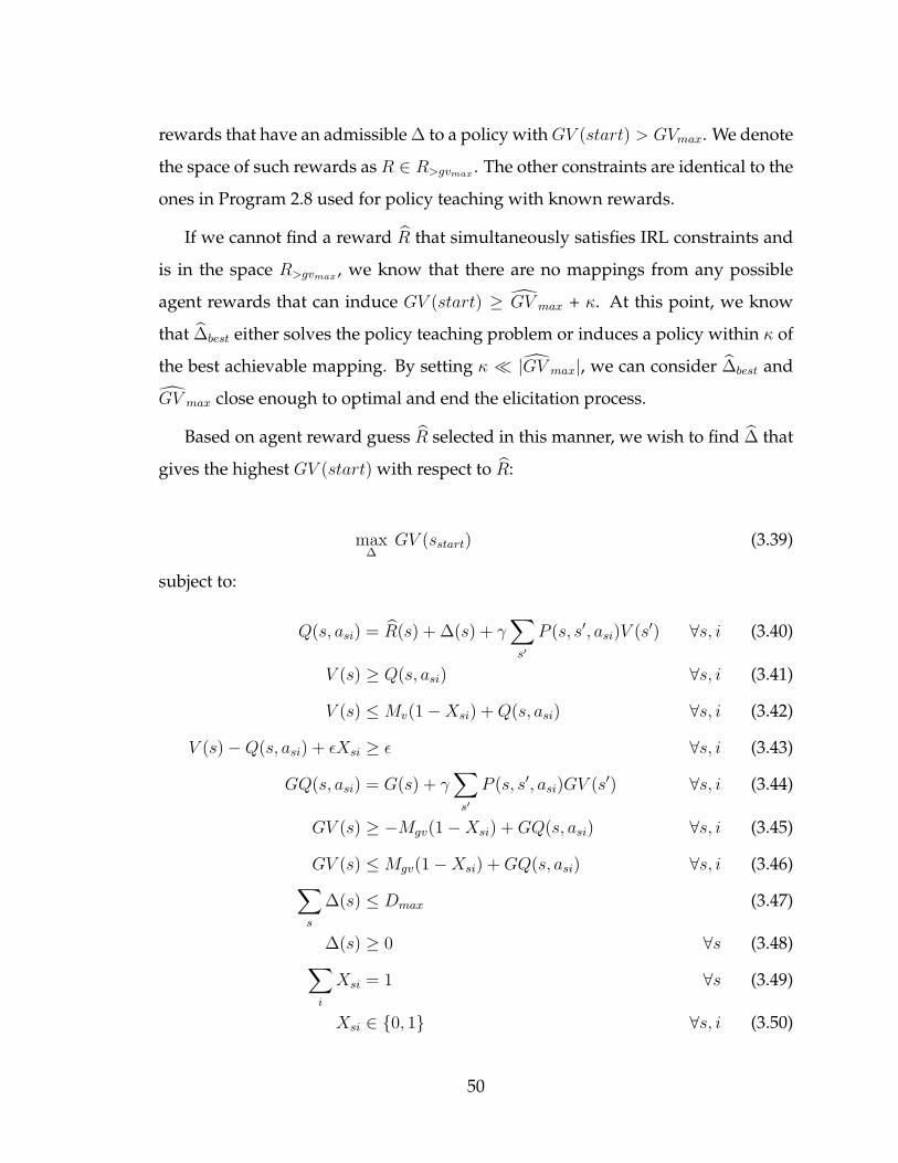
rewards that have an admissible ∆ to a policy with GV (start) > GVmax. We denote

the space of such rewards as R ∈ R>gvmax . The other constraints are identical to the

ones in Program 2.8 used for policy teaching with known rewards.

If we cannot find a reward R that simultaneously satisfies IRL constraints and

is in the space R>gvmax , we know that there are no mappings from any possible

agent rewards that can induce GV (start) ≥ GV max + κ. At this point, we know

that ∆best either solves the policy teaching problem or induces a policy within κ of

the best achievable mapping. By setting κ � |GV max|, we can consider ∆best and

GV max close enough to optimal and end the elicitation process.

Based on agent reward guess R selected in this manner, we wish to find ∆ that

gives the highest GV (start) with respect to R:

max∆

GV (sstart) (3.39)

subject to:

Q(s, asi) = R(s) + ∆(s) + γ∑

s′

P (s, s′, asi)V (s′) ∀s, i (3.40)

V (s) ≥ Q(s, asi) ∀s, i (3.41)

V (s) ≤Mv(1−Xsi) + Q(s, asi) ∀s, i (3.42)

V (s)−Q(s, asi) + εXsi ≥ ε ∀s, i (3.43)

GQ(s, asi) = G(s) + γ∑

s′

P (s, s′, asi)GV (s′) ∀s, i (3.44)

GV (s) ≥ −Mgv(1−Xsi) + GQ(s, asi) ∀s, i (3.45)

GV (s) ≤Mgv(1−Xsi) + GQ(s, asi) ∀s, i (3.46)∑s

∆(s) ≤ Dmax (3.47)

∆(s) ≥ 0 ∀s (3.48)∑i

Xsi = 1 ∀s (3.49)

Xsi ∈ {0, 1} ∀s, i (3.50)

50

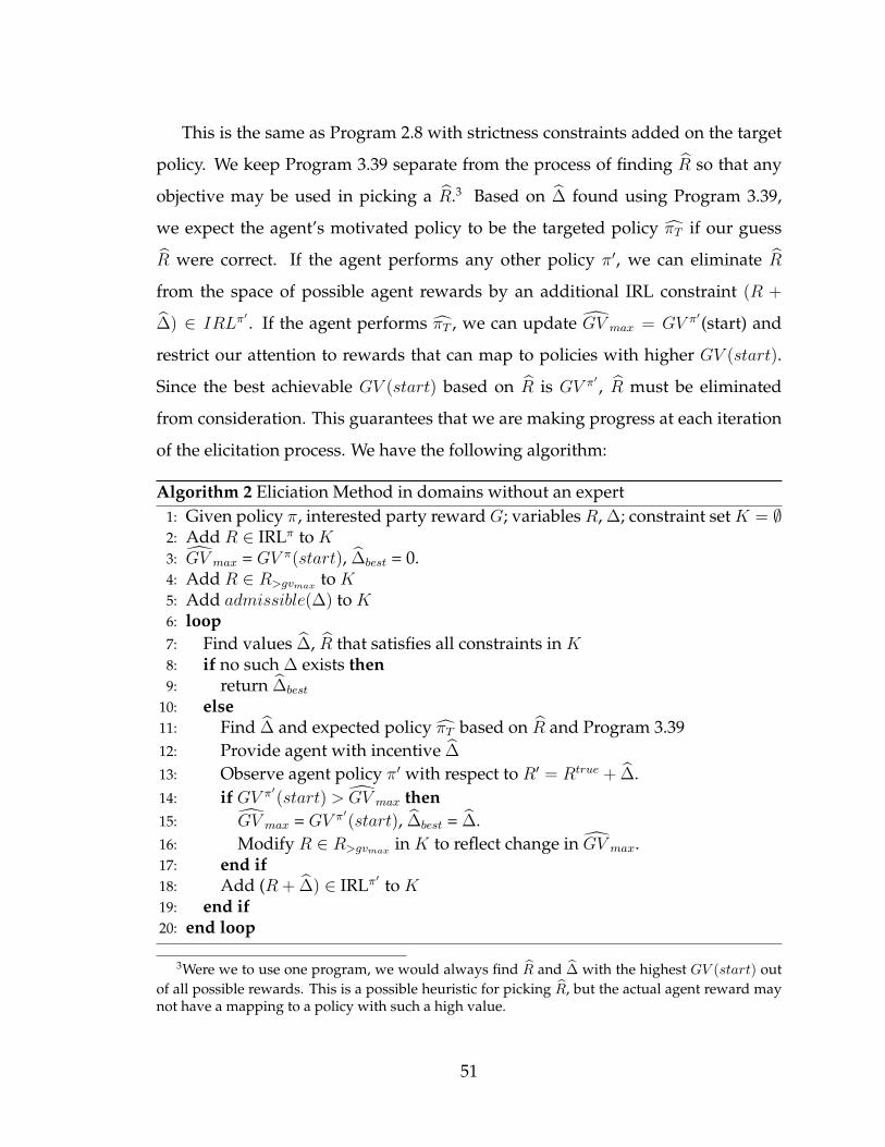
This is the same as Program 2.8 with strictness constraints added on the target

policy. We keep Program 3.39 separate from the process of finding R so that any

objective may be used in picking a R.3 Based on ∆ found using Program 3.39,

we expect the agent’s motivated policy to be the targeted policy πT if our guess

R were correct. If the agent performs any other policy π′, we can eliminate R

from the space of possible agent rewards by an additional IRL constraint (R +

∆) ∈ IRLπ′ . If the agent performs πT , we can update GV max = GV π′(start) and

restrict our attention to rewards that can map to policies with higher GV (start).

Since the best achievable GV (start) based on R is GV π′ , R must be eliminated

from consideration. This guarantees that we are making progress at each iteration

of the elicitation process. We have the following algorithm:

Algorithm 2 Eliciation Method in domains without an expert1: Given policy π, interested party reward G; variables R, ∆; constraint set K = ∅2: Add R ∈ IRLπ to K3: GV max = GV π(start), ∆best = 0.4: Add R ∈ R>gvmax to K5: Add admissible(∆) to K6: loop7: Find values ∆, R that satisfies all constraints in K8: if no such ∆ exists then9: return ∆best

10: else11: Find ∆ and expected policy πT based on R and Program 3.3912: Provide agent with incentive ∆

13: Observe agent policy π′ with respect to R′ = Rtrue + ∆.14: if GV π′

(start) > GV max then15: GV max = GV π′

(start), ∆best = ∆.16: Modify R ∈ R>gvmax in K to reflect change in GV max.17: end if18: Add (R + ∆) ∈ IRLπ′ to K19: end if20: end loop

3Were we to use one program, we would always find R and ∆ with the highest GV (start) outof all possible rewards. This is a possible heuristic for picking R, but the actual agent reward maynot have a mapping to a policy with such a high value.

51

Algorithm 2 formalizes the elicitation process for domains without an expert.

At every iteration, we add an IRL constraint based on π′ whether π′ = πT or not;

this ensures that we incorporate any evidence gathered even if a generated con-

straint is not guaranteed to eliminate points from the space. We make the same

kind of completion guarantee as we make with Algorithm 1:

Theorem 4. Algorithm 2 terminates in a finite number of steps with an admissible ∆ that

maps to a policy whose GV(start) is within κ of the maximium GV(start) achievable with

respect to the agent’s true reward.

Proof. Every iteration of Algorithm 2 finds R and ∆ that strictly induces a policy

πT with slack of at least ε. If the agent performs a policy π′ 6= πT , the added IRL

constraint R + ∆ ∈ IRLπ′ ensures that R and all points within an open hypercube

with side length 2δ = ε(1−γ)γ

centered at R are not the agent’s reward function. If

π′ = πT , GV max increases. Since Program 3.39 ensured that ∆ mapped R to its

highest achievable GV (start), the constraints R>gvmax ensure that R and all points

within an open hypercube with side length 2δ = ε(1−γ)γ

centered at R are not the

agent’s reward function. It follows by an application of Lemma 5 that only a finite

number of R need to be eliminated in order to cover the space of possible agent

rewards. Since Algorithm 2 only terminates when there is no possible agent re-

ward that can achieve a GV (start) of at least GV max +κ, the returned admissible ∆

maps the agent’s true reward to a policy with GV (start) within κ of the maximum

achievable GV (start) with respect to the agent’s true reward.

3.2.5 Elicitation Objective Function

Algorithms 1 and 2 allow us to solve the policy teaching problem with unknown

rewards using general elicitation methods that are guaranteed to terminate within

a finite number of steps. The methods allow for any objective function to be used

for choosing R and ∆ that satisfy the constraints on R and ∆. In choosing an

objective function, we are interested in the following properties:

52

• Few elicitation rounds in practice

While we have guarantees on the maximum number of rounds that the elici-

tation process may take, we wish to complete the elicitation process in as few

rounds as possible. In domains without an expert, we need to solve com-

putationally expensive Mixed Integer Programs at every iteration. In both

domains with and without an expert, we wish to limit the amount of interac-

tion we need to have with the agent before finding a solution.

• Robustness

In cases where elicitation is lengthy or costly, we may wish to perform only

a couple of rounds of elicitation and return the best mapping found before

the policy teaching problem is solved. In these situations, choosing potential

mappings that can guarantee a certain level of GV(start) with respect to un-

certainty over the agent’s rewards may be more important than reducing the

number of elicitation rounds.

• Tractability

Objective functions that satisfy the above properties must be computation-

ally tractable to be applicable in practice.

These properties are all desirable, but any particular objective function is un-

likely to achieve all three. In some cases, there may be heuristics that do not make

guarantees but perform well in practice. We will discuss the minimax regret crite-

rion for guarantees on the quality of induced policies and methods of cutting the

reward space to reduce the number of elicitation rounds.

Minimax Regret

The minimax regret decision criterion provides a method of making robust deci-

sions. The criterion bounds the worst case error in making a decision given uncer-

tainty over preferences. The criterion does not require a prior over possible agent

53

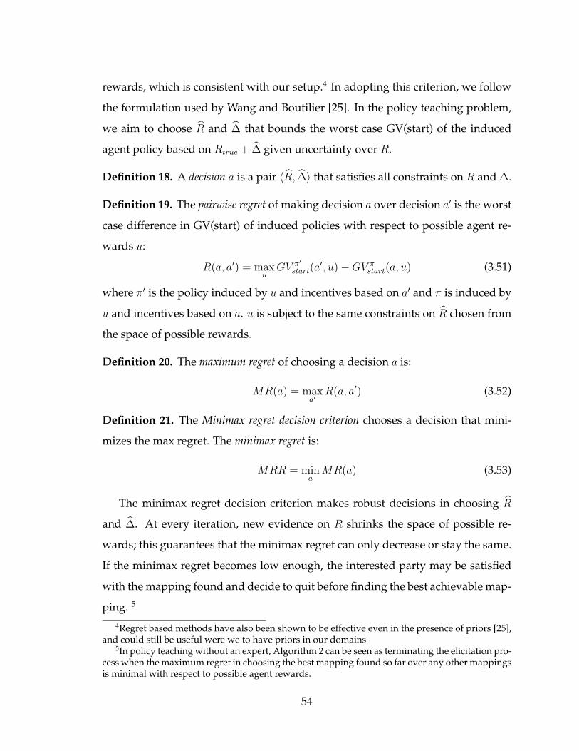
rewards, which is consistent with our setup.4 In adopting this criterion, we follow

the formulation used by Wang and Boutilier [25]. In the policy teaching problem,

we aim to choose R and ∆ that bounds the worst case GV(start) of the induced

agent policy based on Rtrue + ∆ given uncertainty over R.

Definition 18. A decision a is a pair 〈R, ∆〉 that satisfies all constraints on R and ∆.

Definition 19. The pairwise regret of making decision a over decision a′ is the worst

case difference in GV(start) of induced policies with respect to possible agent re-

wards u:

R(a, a′) = maxu

GV π′

start(a′, u)−GV π

start(a, u) (3.51)

where π′ is the policy induced by u and incentives based on a′ and π is induced by

u and incentives based on a. u is subject to the same constraints on R chosen from

the space of possible rewards.

Definition 20. The maximum regret of choosing a decision a is:

MR(a) = maxa′

R(a, a′) (3.52)

Definition 21. The Minimax regret decision criterion chooses a decision that mini-

mizes the max regret. The minimax regret is:

MRR = mina

MR(a) (3.53)

The minimax regret decision criterion makes robust decisions in choosing R

and ∆. At every iteration, new evidence on R shrinks the space of possible re-

wards; this guarantees that the minimax regret can only decrease or stay the same.

If the minimax regret becomes low enough, the interested party may be satisfied

with the mapping found and decide to quit before finding the best achievable map-

ping. 5

4Regret based methods have also been shown to be effective even in the presence of priors [25],and could still be useful were we to have priors in our domains

5In policy teaching without an expert, Algorithm 2 can be seen as terminating the elicitation pro-cess when the maximum regret in choosing the best mapping found so far over any other mappingsis minimal with respect to possible agent rewards.

54

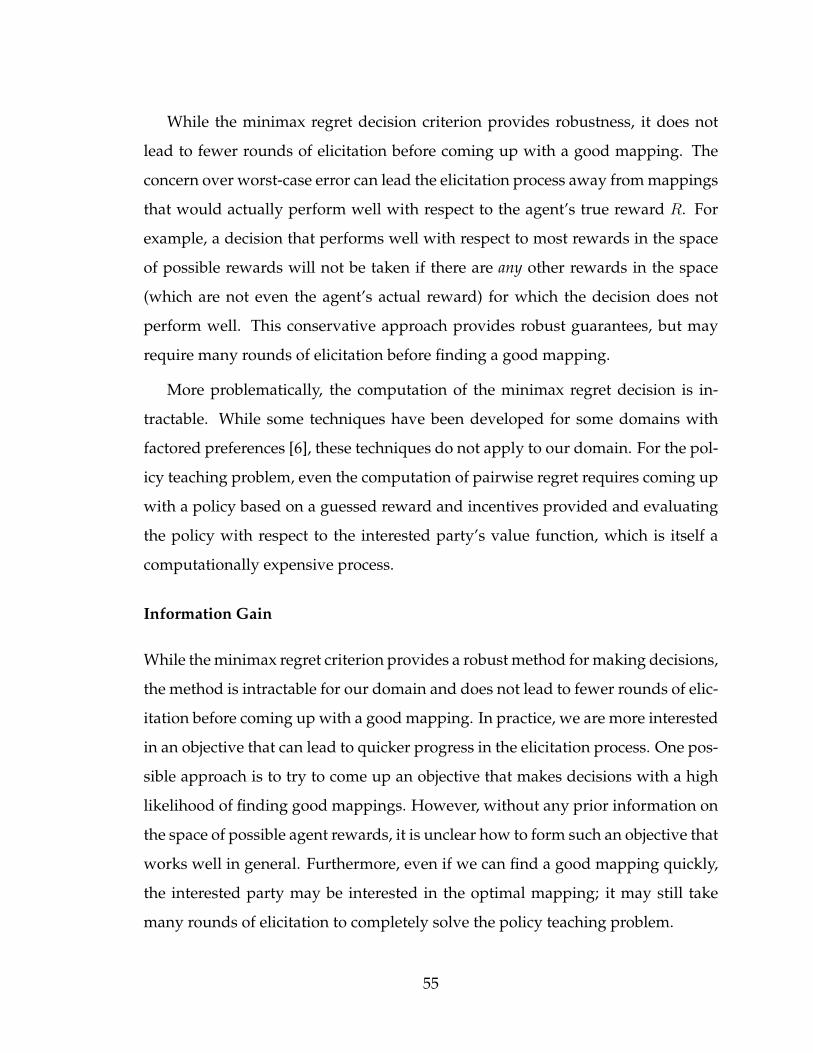
While the minimax regret decision criterion provides robustness, it does not

lead to fewer rounds of elicitation before coming up with a good mapping. The

concern over worst-case error can lead the elicitation process away from mappings

that would actually perform well with respect to the agent’s true reward R. For

example, a decision that performs well with respect to most rewards in the space

of possible rewards will not be taken if there are any other rewards in the space

(which are not even the agent’s actual reward) for which the decision does not

perform well. This conservative approach provides robust guarantees, but may

require many rounds of elicitation before finding a good mapping.

More problematically, the computation of the minimax regret decision is in-

tractable. While some techniques have been developed for some domains with

factored preferences [6], these techniques do not apply to our domain. For the pol-

icy teaching problem, even the computation of pairwise regret requires coming up

with a policy based on a guessed reward and incentives provided and evaluating

the policy with respect to the interested party’s value function, which is itself a

computationally expensive process.

Information Gain

While the minimax regret criterion provides a robust method for making decisions,

the method is intractable for our domain and does not lead to fewer rounds of elic-

itation before coming up with a good mapping. In practice, we are more interested

in an objective that can lead to quicker progress in the elicitation process. One pos-

sible approach is to try to come up an objective that makes decisions with a high

likelihood of finding good mappings. However, without any prior information on

the space of possible agent rewards, it is unclear how to form such an objective that

works well in general. Furthermore, even if we can find a good mapping quickly,

the interested party may be interested in the optimal mapping; it may still take

many rounds of elicitation to completely solve the policy teaching problem.

55

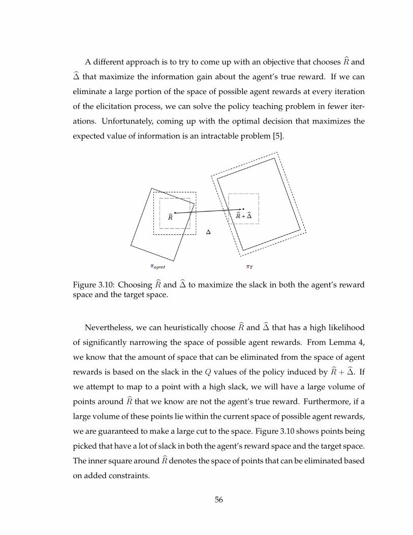
A different approach is to try to come up with an objective that chooses R and

∆ that maximize the information gain about the agent’s true reward. If we can

eliminate a large portion of the space of possible agent rewards at every iteration

of the elicitation process, we can solve the policy teaching problem in fewer iter-

ations. Unfortunately, coming up with the optimal decision that maximizes the

expected value of information is an intractable problem [5].

Figure 3.10: Choosing R and ∆ to maximize the slack in both the agent’s rewardspace and the target space.

Nevertheless, we can heuristically choose R and ∆ that has a high likelihood

of significantly narrowing the space of possible agent rewards. From Lemma 4,

we know that the amount of space that can be eliminated from the space of agent

rewards is based on the slack in the Q values of the policy induced by R + ∆. If

we attempt to map to a point with a high slack, we will have a large volume of

points around R that we know are not the agent’s true reward. Furthermore, if a

large volume of these points lie within the current space of possible agent rewards,

we are guaranteed to make a large cut to the space. Figure 3.10 shows points being

picked that have a lot of slack in both the agent’s reward space and the target space.

The inner square around R denotes the space of points that can be eliminated based

on added constraints.

56

In coming up with an objective, we aim to maximize both the slack on the

agent’s policy based on R and the slack around the target policy based on R + ∆.

In domains with an expert, the target policy is the expert’s policy πE , and the slack

is based on a reward RE ∈ IRLπEstrict. We can write down the objective and the

associated constraints with a simple linear program:

max∆

[∑

s

β(s) +∑

s

βE(s)− λ∑

s

α(s)] (3.54)

α(s) ≥ R(s) ∀s ∈ S (3.55)

α(s) ≥ −R(s) ∀s ∈ S (3.56)

((Pπ −Pa)(I− γPπ)−1R)[s] ≥ β(s) ∀a ∈ A, s ∈ S (3.57)

((PπE−Pa)(I− γPπE

)−1RE)[s] ≥ βE(s) ∀a ∈ A, s ∈ S (3.58)

(Pπ −Pa)(I− γPπ)−1R � 0 ∀a ∈ A (3.59)

(PπE−Pa)(I− γPπE

)−1RE � ε ∀a ∈ A (3.60)∑s

∆(s) ≤ Dmax (3.61)

∆(s) ≥ 0 ∀s (3.62)

where β is the slack in the agent’s Q values, βE is the slack in the expert’s Q values,

and α is the absolute value of the picked agent reward. The λ constant and the

α variables place a weighted penalty on large rewards, which allows us to prefer

simpler rewards and also to avoid picking large rewards for the sake of increasing

the slack.6 While this program does not provide any guarantees like minimax re-

gret, it is a tractable linear program that is likely to significantly reduce the number

of iterations in the elicitation process.

We can similarly attempt to maximize the slack for problems in domains with-

out an expert. In these domains, R and ∆ are chosen separately; an optimization

problem that simultaneously finds a 〈R, ∆〉 pair with the highest stack and ensures6If we wish, we can place penalty terms on the expert’s reward as well. We can also place

additional constraints to weigh or balance the values of β and βE .

57

that ∆ maps R to a policy with the highest achievable GV(start) is computationally

intractable. However, we can achieve much of the same effect by using one of the

following tractable alternatives:

1. Choose R with maximal slack for the agent’s policy. Find highest reach-

able GV max based on R. Find ∆ with maximal slack such that R + ∆ has

GV (start) = GV max.

2. Find highest achievable GV max based on any R and ∆. Find R and ∆ with

maximal slack such that R + ∆ has GV (start) = GV max.

3. Find R and ∆ with maximal slack without requiring ∆ to map R to the best

achievable policy. Based on R, find a ∆ with maximal slack such that R + ∆

has GV(start) = GV max.

The first alternative provides a greedy method by finding R with maximal slack

and then finding ∆ with maximal slack based on R. The second alternative restricts

attention to R that can induce a policy with the highest GV(start) and maximizes

the slack within this subset of R’s. The third alternative chooses R hoping that

the ∆ that provides maximal slack is one that induces the policy with the highest

GV(start), and then picks ∆ with maximal slack based on this R.

We will adopt the first alternative here because it is less restrictive than the

second alternative and more robust than the third. The first alternative is also likely

to perform well because it picks R with a large slack such that points around R to

be eliminated are still within the space of possible agent rewards. This guarantees

that as much progress is made as points eliminated by added constraints.

In choosing R, we ensure R ∈ IRLπ, R ∈ R>gvmax , and add additional IRL

constraints based on observed induced policies. We use the following objective,

with the same β and α constraints in domains with an expert to capture the slack

in Q values and to penalize large rewards, respectively:

58

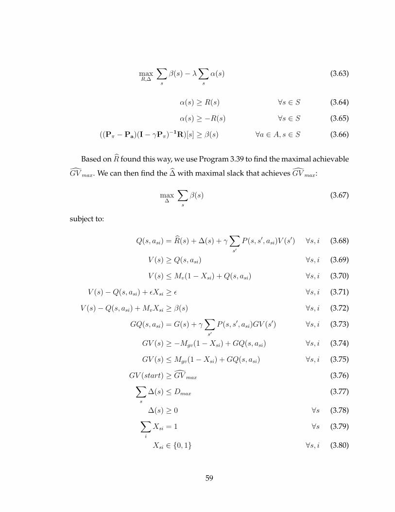
maxR,∆

∑s

β(s)− λ∑

s

α(s) (3.63)

α(s) ≥ R(s) ∀s ∈ S (3.64)

α(s) ≥ −R(s) ∀s ∈ S (3.65)

((Pπ −Pa)(I− γPπ)−1R)[s] ≥ β(s) ∀a ∈ A, s ∈ S (3.66)

Based on R found this way, we use Program 3.39 to find the maximal achievable

GV max. We can then find the ∆ with maximal slack that achieves GV max:

max∆

∑s

β(s) (3.67)

subject to:

Q(s, asi) = R(s) + ∆(s) + γ∑

s′

P (s, s′, asi)V (s′) ∀s, i (3.68)

V (s) ≥ Q(s, asi) ∀s, i (3.69)

V (s) ≤Mv(1−Xsi) + Q(s, asi) ∀s, i (3.70)

V (s)−Q(s, asi) + εXsi ≥ ε ∀s, i (3.71)

V (s)−Q(s, asi) + MvXsi ≥ β(s) ∀s, i (3.72)

GQ(s, asi) = G(s) + γ∑

s′

P (s, s′, asi)GV (s′) ∀s, i (3.73)

GV (s) ≥ −Mgv(1−Xsi) + GQ(s, asi) ∀s, i (3.74)

GV (s) ≤Mgv(1−Xsi) + GQ(s, asi) ∀s, i (3.75)

GV (start) ≥ GV max (3.76)∑s

∆(s) ≤ Dmax (3.77)

∆(s) ≥ 0 ∀s (3.78)∑i

Xsi = 1 ∀s (3.79)

Xsi ∈ {0, 1} ∀s, i (3.80)

59

where the constants are set as in Program 3.39. Constraint 3.72 ensures that β

captures the minimal slack between the optimal action taken and all other actions,

and Constraint 3.76 ensures that we find solutions with GV(start) at least GV max.

The slack maximizing heuristics we have proposed for domains with and with-

out an expert do not introduce additional computational complexity, but have a

high potential for decreasing the number of rounds of elicitation necessary before

finding a solution. But how well do these heuristics work in practice? To use these

heuristics and our elicitation algorithms, also we need to set the minimal slack ε

and the reward penalty λ. How should we set these values, and what effects do

they have on the length of the elicitation process?

60

Chapter 4

Experiments

4.1 Experiments

4.1.1 Experimental Setup

We implemented Algorithm 1 and Algorithm 2 with the slack maximizing heuris-

tics introduced in Subsection 3.2.5 to evaluate the performance of our algorithms

on our motivating example. We also implemented methods for policy teaching

with known rewards as a way of determining whether any feasible mappings ex-

ists based on true rewards and the limits on ∆. We used CPLEX version 10.1 to

solve the linear programs and mixed integer programs in our algorithms. Our

code is written in Java, and uses JOpt1 as a Java inteface to CPLEX. Experiments

are conducted on a local machine with a 2.4Ghz processor and 512MB of RAM.

4.1.2 Setting Parameters

The policy teaching algorithms and the heuristics we use require us to set a couple

of parameters. In setting the ε for the minimal slack in Q values of policies mapped

to, we aim to set the largest value for which we are almost certain we can find a

mapping if one exists. To do this, we consider the largest possible increase in ∆

that needs to be added for there to be a mapping with a slack of ε given that there

1http://econcs.eecs.harvard.edu/jopt

61

exists an admissible mapping. The slack corresponds to a reward pertubation of

at most ε(1−γ)2γ

in each state; for a domain with n states, the maximal amount of ∆

we may need to have to add is δ+ = nε(1−γ)2γ

. If we can set ε such that δ+ is a small

percentage of Dmax (i.e. 1%), we are almost certain that there will be a mapping

with slack ε if there is an admissible mapping.2

For our slack maximizing objective functions, we need to set the reward penal-

izing coefficient λ. As we have briefly mentioned, penalty terms on the reward

function allow the objective to prefer “simpler” rewards and avoid choosing large

rewards for the sake of increasing the slack. Simple rewards provide a simple

explanation for the agent’s behavior. Without any penalty terms, the objective is

likely to add bumps to the reward function that would increase the slack but do

little extra to explain the agent’s behavior. While this seems to suggest that we

should set λ to be large, we do not want to set λ to be so large as to focus on

penalizing rewards over maximizing the slack that our heuristic depends on for

increasing the information gain.

Ng and Russell [16] observed that since R = 0 is always a solution to (nonstrict)

IRL constraints, for large enough λ, the penalty on rewards would cause R = 0 to

be the solution to the slack maximizing objective in Program 3.17.3 They proposed

choosing the “simplest” non-zero R by setting λ right below the phase transition

λ0, where R 6= 0 for λ < λ0, and R = 0 for λ > λ0. Setting λ this way provides a

natural way of picking rewards, and avoids having to hand-tune the parameter.

However, λ set this way is unlikely to be a good choice for the policy teaching

problem. First, setting λ right below the phase transition produces smooth reward

functions with zero rewards in most states. For Ng and Russell’s problem domain,

this provides a fine choice because they aimed to recover a simple and generaliz-

able reward function. For the policy teaching problem where an agent is likely to2δ+ is based on a worst case analysis. Setting it at 1% of Dmax is a conservative estimate.3The objective has value 0 when R = 0. Our objectives in our heuristics are slightly different and

do not have this property, as we deal with expert policies (with strictness constraints preventingRE = 0) in one objective and GVmax constraints for domains without an expert.

62

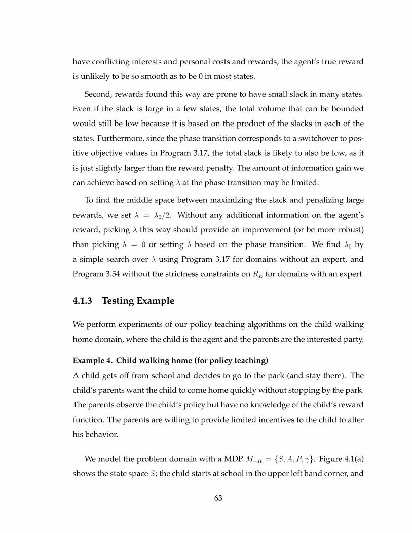
have conflicting interests and personal costs and rewards, the agent’s true reward

is unlikely to be so smooth as to be 0 in most states.

Second, rewards found this way are prone to have small slack in many states.

Even if the slack is large in a few states, the total volume that can be bounded

would still be low because it is based on the product of the slacks in each of the

states. Furthermore, since the phase transition corresponds to a switchover to pos-

itive objective values in Program 3.17, the total slack is likely to also be low, as it

is just slightly larger than the reward penalty. The amount of information gain we

can achieve based on setting λ at the phase transition may be limited.

To find the middle space between maximizing the slack and penalizing large

rewards, we set λ = λ0/2. Without any additional information on the agent’s

reward, picking λ this way should provide an improvement (or be more robust)

than picking λ = 0 or setting λ based on the phase transition. We find λ0 by

a simple search over λ using Program 3.17 for domains without an expert, and

Program 3.54 without the strictness constraints on RE for domains with an expert.

4.1.3 Testing Example

We perform experiments of our policy teaching algorithms on the child walking

home domain, where the child is the agent and the parents are the interested party.

Example 4. Child walking home (for policy teaching)

A child gets off from school and decides to go to the park (and stay there). The

child’s parents want the child to come home quickly without stopping by the park.

The parents observe the child’s policy but have no knowledge of the child’s reward

function. The parents are willing to provide limited incentives to the child to alter

his behavior.

We model the problem domain with a MDP M−R = {S, A, P, γ}. Figure 4.1(a)

shows the state space S; the child starts at school in the upper left hand corner, and

63

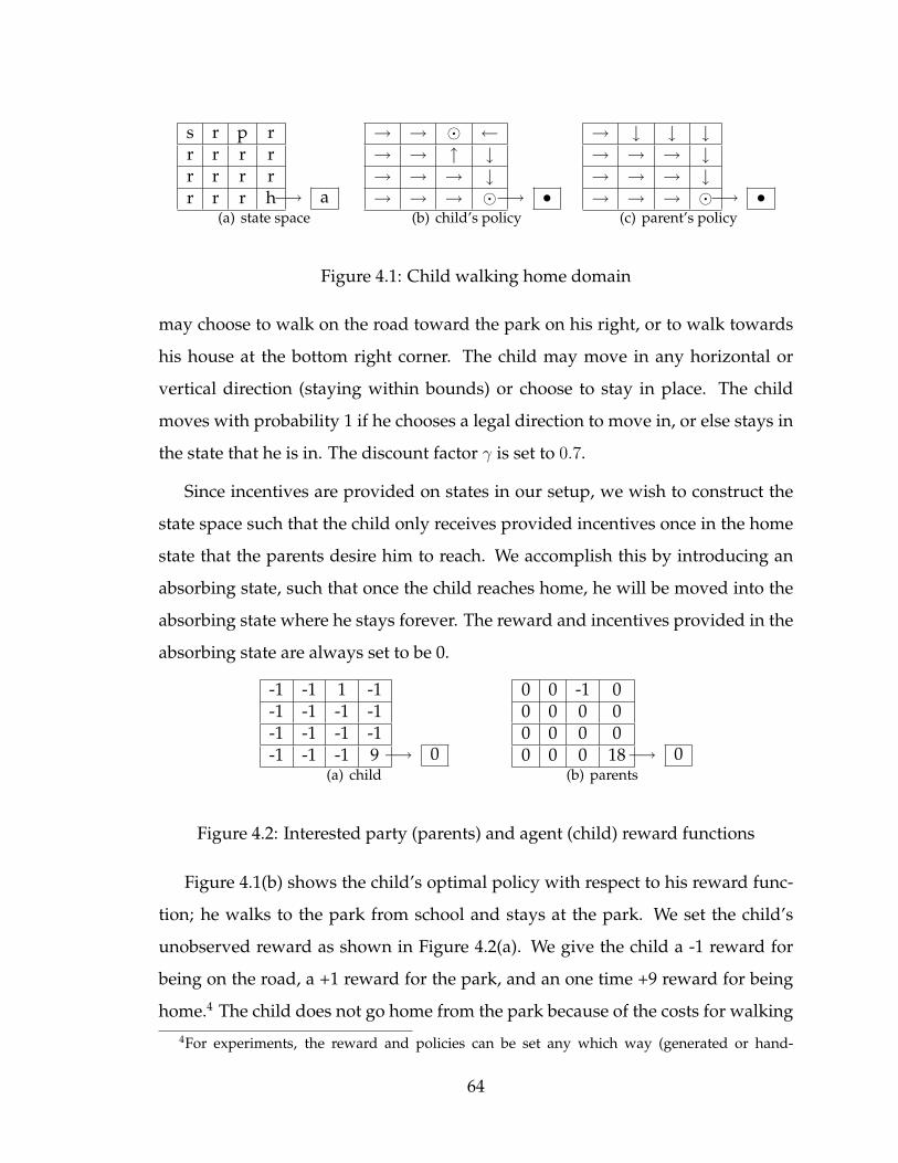
s r p rr r r rr r r rr r r h−→ a

(a) state space

→ → � ←→ → ↑ ↓→ → → ↓→ → → �−→ •

(b) child’s policy

→ ↓ ↓ ↓→ → → ↓→ → → ↓→ → → �−→ •

(c) parent’s policy

Figure 4.1: Child walking home domain

may choose to walk on the road toward the park on his right, or to walk towards

his house at the bottom right corner. The child may move in any horizontal or

vertical direction (staying within bounds) or choose to stay in place. The child

moves with probability 1 if he chooses a legal direction to move in, or else stays in

the state that he is in. The discount factor γ is set to 0.7.

Since incentives are provided on states in our setup, we wish to construct the

state space such that the child only receives provided incentives once in the home

state that the parents desire him to reach. We accomplish this by introducing an

absorbing state, such that once the child reaches home, he will be moved into the

absorbing state where he stays forever. The reward and incentives provided in the

absorbing state are always set to be 0.

-1 -1 1 -1-1 -1 -1 -1-1 -1 -1 -1-1 -1 -1 9 −→ 0

(a) child

0 0 -1 00 0 0 00 0 0 00 0 0 18−→ 0

(b) parents

Figure 4.2: Interested party (parents) and agent (child) reward functions

Figure 4.1(b) shows the child’s optimal policy with respect to his reward func-

tion; he walks to the park from school and stays at the park. We set the child’s

unobserved reward as shown in Figure 4.2(a). We give the child a -1 reward for

being on the road, a +1 reward for the park, and an one time +9 reward for being

home.4 The child does not go home from the park because of the costs for walking4For experiments, the reward and policies can be set any which way (generated or hand-

64

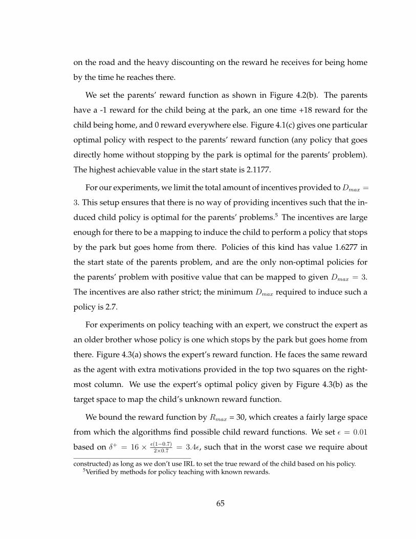
on the road and the heavy discounting on the reward he receives for being home

by the time he reaches there.

We set the parents’ reward function as shown in Figure 4.2(b). The parents

have a -1 reward for the child being at the park, an one time +18 reward for the

child being home, and 0 reward everywhere else. Figure 4.1(c) gives one particular

optimal policy with respect to the parents’ reward function (any policy that goes

directly home without stopping by the park is optimal for the parents’ problem).

The highest achievable value in the start state is 2.1177.

For our experiments, we limit the total amount of incentives provided to Dmax =

3. This setup ensures that there is no way of providing incentives such that the in-

duced child policy is optimal for the parents’ problems.5 The incentives are large

enough for there to be a mapping to induce the child to perform a policy that stops

by the park but goes home from there. Policies of this kind has value 1.6277 in

the start state of the parents problem, and are the only non-optimal policies for

the parents’ problem with positive value that can be mapped to given Dmax = 3.

The incentives are also rather strict; the minimum Dmax required to induce such a

policy is 2.7.

For experiments on policy teaching with an expert, we construct the expert as

an older brother whose policy is one which stops by the park but goes home from

there. Figure 4.3(a) shows the expert’s reward function. He faces the same reward

as the agent with extra motivations provided in the top two squares on the right-

most column. We use the expert’s optimal policy given by Figure 4.3(b) as the

target space to map the child’s unknown reward function.

We bound the reward function by Rmax = 30, which creates a fairly large space

from which the algorithms find possible child reward functions. We set ε = 0.01

based on δ+ = 16 × ε(1−0.7)2×0.7

= 3.4ε, such that in the worst case we require about

constructed) as long as we don’t use IRL to set the true reward of the child based on his policy.5Verified by methods for policy teaching with known rewards.

65

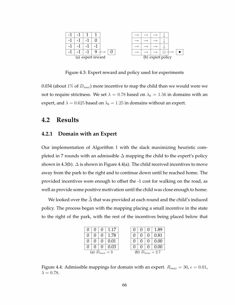
-1 -1 1 1-1 -1 -1 0-1 -1 -1 -1-1 -1 -1 9 −→ 0

(a) expert reward

→ → → ↓→ → → ↓→ → → ↓→ → → �−→ •

(b) expert policy

Figure 4.3: Expert reward and policy used for experiments

0.034 (about 1% of Dmax) more incentive to map the child than we would were we

not to require strictness. We set λ = 0.78 based on λ0 = 1.56 in domains with an

expert, and λ = 0.625 based on λ0 = 1.25 in domains without an expert.

4.2 Results

4.2.1 Domain with an Expert

Our implementation of Algorithm 1 with the slack maximizing heuristic com-

pleted in 7 rounds with an admissible ∆ mapping the child to the expert’s policy

shown in 4.3(b). ∆ is shown in Figure 4.4(a). The child received incentives to move

away from the park to the right and to continue down until he reached home. The

provided incentives were enough to offset the -1 cost for walking on the road, as

well as provide some positive motivation until the child was close enough to home.

We looked over the ∆ that was provided at each round and the child’s induced

policy. The process began with the mapping placing a small incentive in the state

to the right of the park, with the rest of the incentives being placed below that

0 0 0 1.170 0 0 1.780 0 0 0.010 0 0 0.03

(a) Dmax = 3

0 0 0 1.890 0 0 0.810 0 0 0.000 0 0 0.00(b) Dmax = 2.7

Figure 4.4: Admissible mappings for domain with an expert. Rmax = 30, ε = 0.01,λ = 0.78.

66

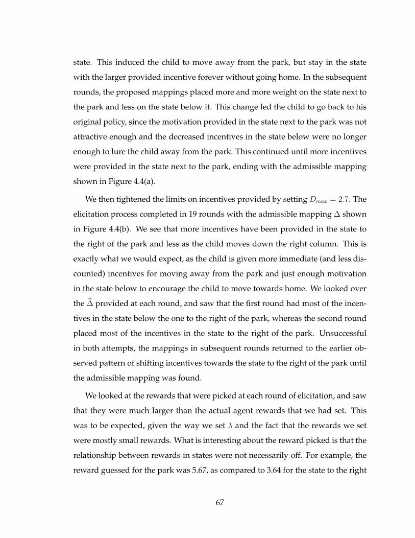
state. This induced the child to move away from the park, but stay in the state

with the larger provided incentive forever without going home. In the subsequent

rounds, the proposed mappings placed more and more weight on the state next to

the park and less on the state below it. This change led the child to go back to his

original policy, since the motivation provided in the state next to the park was not

attractive enough and the decreased incentives in the state below were no longer

enough to lure the child away from the park. This continued until more incentives

were provided in the state next to the park, ending with the admissible mapping

shown in Figure 4.4(a).

We then tightened the limits on incentives provided by setting Dmax = 2.7. The

elicitation process completed in 19 rounds with the admissible mapping ∆ shown

in Figure 4.4(b). We see that more incentives have been provided in the state to

the right of the park and less as the child moves down the right column. This is

exactly what we would expect, as the child is given more immediate (and less dis-

counted) incentives for moving away from the park and just enough motivation

in the state below to encourage the child to move towards home. We looked over

the ∆ provided at each round, and saw that the first round had most of the incen-

tives in the state below the one to the right of the park, whereas the second round

placed most of the incentives in the state to the right of the park. Unsuccessful

in both attempts, the mappings in subsequent rounds returned to the earlier ob-

served pattern of shifting incentives towards the state to the right of the park until

the admissible mapping was found.

We looked at the rewards that were picked at each round of elicitation, and saw

that they were much larger than the actual agent rewards that we had set. This

was to be expected, given the way we set λ and the fact that the rewards we set

were mostly small rewards. What is interesting about the reward picked is that the

relationship between rewards in states were not necessarily off. For example, the

reward guessed for the park was 5.67, as compared to 3.64 for the state to the right

67

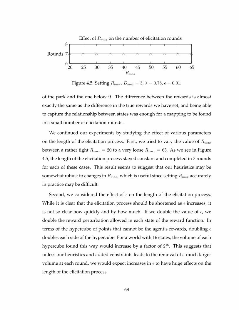
6

7

8

20 25 30 35 40 45 50 55 60 65

Rounds

Rmax

Effect of Rmax on the number of elicitation rounds

4 4 4 4 4 4 4 4 4 4

Figure 4.5: Setting Rmax. Dmax = 3, λ = 0.78, ε = 0.01.

of the park and the one below it. The difference between the rewards is almost

exactly the same as the difference in the true rewards we have set, and being able

to capture the relationship between states was enough for a mapping to be found

in a small number of elicitation rounds.

We continued our experiments by studying the effect of various parameters

on the length of the elicitation process. First, we tried to vary the value of Rmax

between a rather tight Rmax = 20 to a very loose Rmax = 65. As we see in Figure

4.5, the length of the elicitation process stayed constant and completed in 7 rounds

for each of these cases. This result seems to suggest that our heuristics may be

somewhat robust to changes in Rmax, which is useful since setting Rmax accurately

in practice may be difficult.

Second, we considered the effect of ε on the length of the elicitation process.

While it is clear that the elicitation process should be shortened as ε increases, it

is not so clear how quickly and by how much. If we double the value of ε, we

double the reward perturbation allowed in each state of the reward function. In

terms of the hypercube of points that cannot be the agent’s rewards, doubling ε

doubles each side of the hypercube. For a world with 16 states, the volume of each

hypercube found this way would increase by a factor of 216. This suggests that

unless our heuristics and added constraints leads to the removal of a much larger

volume at each round, we would expect increases in ε to have huge effects on the

length of the elicitation process.

68

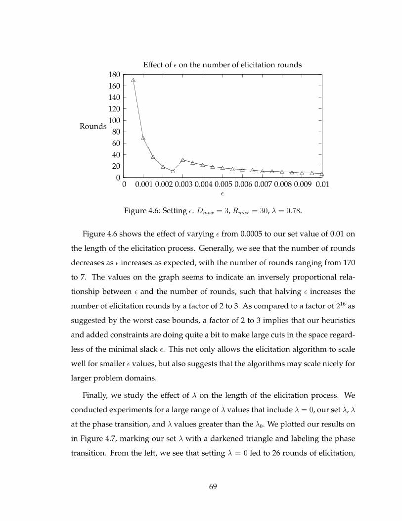
020406080

100120140160180

0 0.001 0.002 0.003 0.004 0.005 0.006 0.007 0.008 0.009 0.01

Rounds

ε

Effect of ε on the number of elicitation rounds

4

4

4

44

4 4 4 4 4 4 4 4 4 4 4 4 4 4 4

Figure 4.6: Setting ε. Dmax = 3, Rmax = 30, λ = 0.78.

Figure 4.6 shows the effect of varying ε from 0.0005 to our set value of 0.01 on

the length of the elicitation process. Generally, we see that the number of rounds

decreases as ε increases as expected, with the number of rounds ranging from 170

to 7. The values on the graph seems to indicate an inversely proportional rela-

tionship between ε and the number of rounds, such that halving ε increases the

number of elicitation rounds by a factor of 2 to 3. As compared to a factor of 216 as

suggested by the worst case bounds, a factor of 2 to 3 implies that our heuristics

and added constraints are doing quite a bit to make large cuts in the space regard-

less of the minimal slack ε. This not only allows the elicitation algorithm to scale

well for smaller ε values, but also suggests that the algorithms may scale nicely for

larger problem domains.

Finally, we study the effect of λ on the length of the elicitation process. We

conducted experiments for a large range of λ values that include λ = 0, our set λ, λ

at the phase transition, and λ values greater than the λ0. We plotted our results on

in Figure 4.7, marking our set λ with a darkened triangle and labeling the phase

transition. From the left, we see that setting λ = 0 led to 26 rounds of elicitation,

69

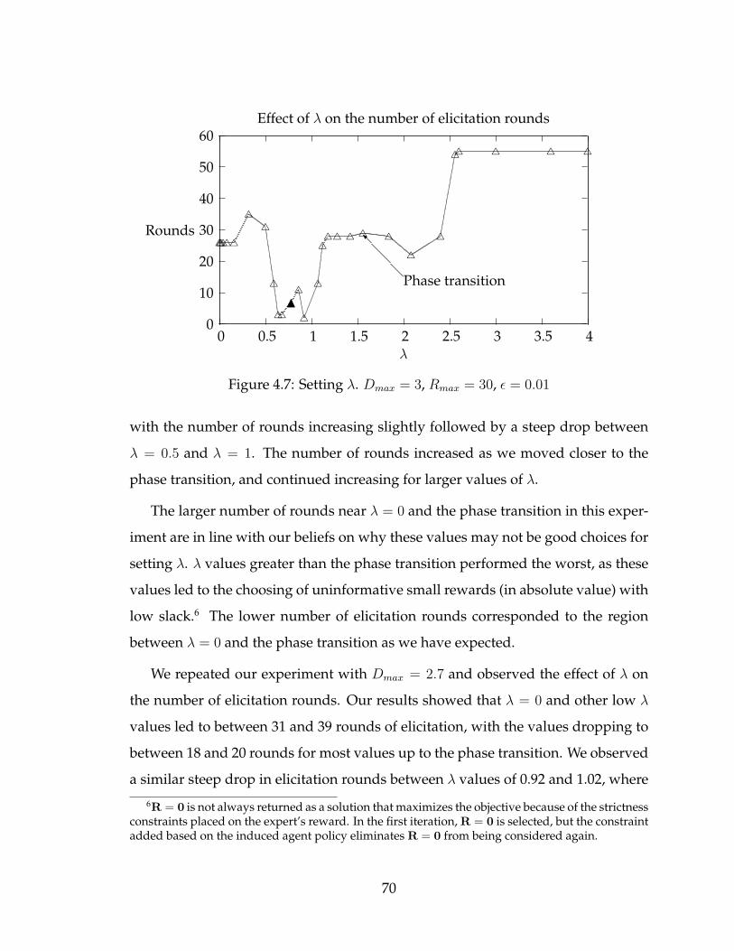
0

10

20

30

40

50

60

0 0.5 1 1.5 2 2.5 3 3.5 4

Rounds

λ

Effect of λ on the number of elicitation rounds

Phase transition

I444444

44

4

44N4

4

4

444 4 4 4

4

4

44 4 4 4

Figure 4.7: Setting λ. Dmax = 3, Rmax = 30, ε = 0.01

with the number of rounds increasing slightly followed by a steep drop between

λ = 0.5 and λ = 1. The number of rounds increased as we moved closer to the

phase transition, and continued increasing for larger values of λ.

The larger number of rounds near λ = 0 and the phase transition in this exper-

iment are in line with our beliefs on why these values may not be good choices for

setting λ. λ values greater than the phase transition performed the worst, as these

values led to the choosing of uninformative small rewards (in absolute value) with

low slack.6 The lower number of elicitation rounds corresponded to the region

between λ = 0 and the phase transition as we have expected.

We repeated our experiment with Dmax = 2.7 and observed the effect of λ on

the number of elicitation rounds. Our results showed that λ = 0 and other low λ

values led to between 31 and 39 rounds of elicitation, with the values dropping to

between 18 and 20 rounds for most values up to the phase transition. We observed

a similar steep drop in elicitation rounds between λ values of 0.92 and 1.02, where

6R = 0 is not always returned as a solution that maximizes the objective because of the strictnessconstraints placed on the expert’s reward. In the first iteration, R = 0 is selected, but the constraintadded based on the induced agent policy eliminates R = 0 from being considered again.

70

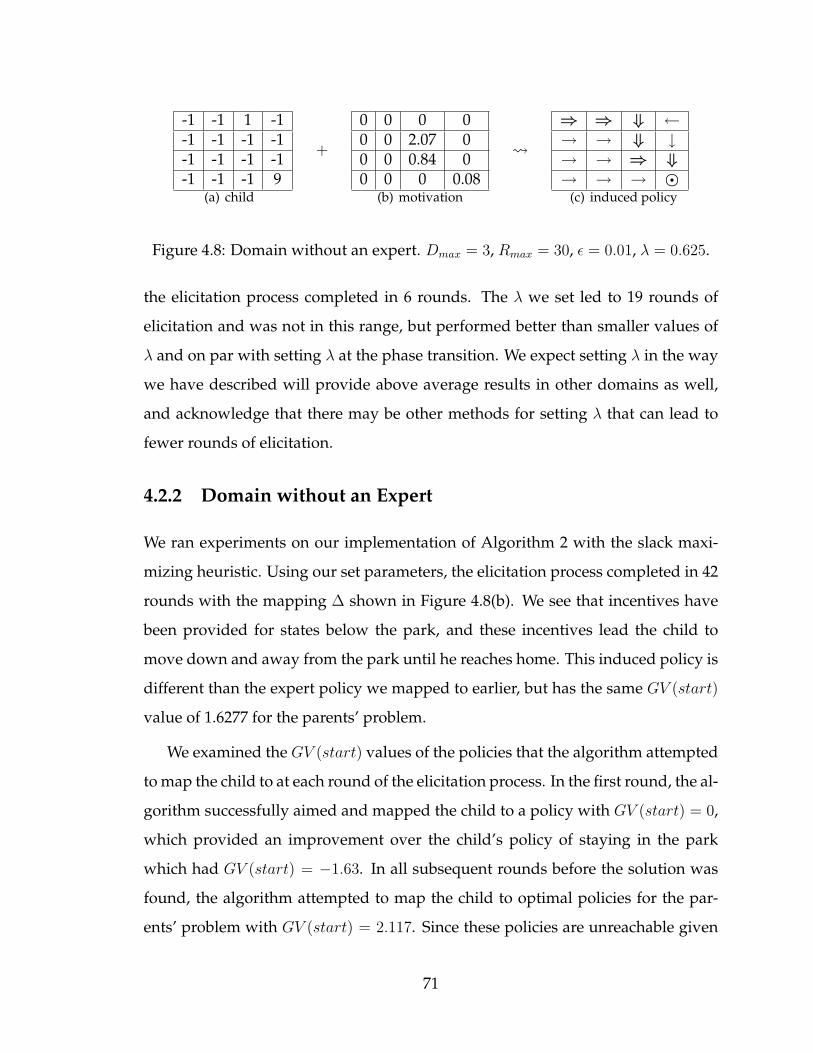
-1 -1 1 -1-1 -1 -1 -1-1 -1 -1 -1-1 -1 -1 9

(a) child

+

0 0 0 00 0 2.07 00 0 0.84 00 0 0 0.08

(b) motivation

⇒ ⇒ ⇓ ←→ → ⇓ ↓→ → ⇒ ⇓→ → → �

(c) induced policy

Figure 4.8: Domain without an expert. Dmax = 3, Rmax = 30, ε = 0.01, λ = 0.625.

the elicitation process completed in 6 rounds. The λ we set led to 19 rounds of

elicitation and was not in this range, but performed better than smaller values of

λ and on par with setting λ at the phase transition. We expect setting λ in the way

we have described will provide above average results in other domains as well,

and acknowledge that there may be other methods for setting λ that can lead to

fewer rounds of elicitation.

4.2.2 Domain without an Expert

We ran experiments on our implementation of Algorithm 2 with the slack maxi-

mizing heuristic. Using our set parameters, the elicitation process completed in 42

rounds with the mapping ∆ shown in Figure 4.8(b). We see that incentives have

been provided for states below the park, and these incentives lead the child to

move down and away from the park until he reaches home. This induced policy is

different than the expert policy we mapped to earlier, but has the same GV (start)

value of 1.6277 for the parents’ problem.

We examined the GV (start) values of the policies that the algorithm attempted

to map the child to at each round of the elicitation process. In the first round, the al-

gorithm successfully aimed and mapped the child to a policy with GV (start) = 0,

which provided an improvement over the child’s policy of staying in the park

which had GV (start) = −1.63. In all subsequent rounds before the solution was

found, the algorithm attempted to map the child to optimal policies for the par-

ents’ problem with GV (start) = 2.117. Since these policies are unreachable given

71

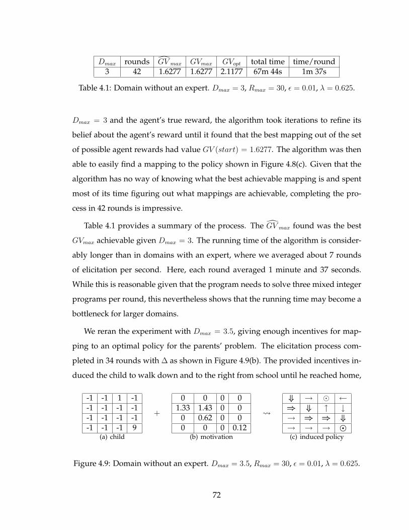
Dmax rounds GV max GVmax GVopt total time time/round3 42 1.6277 1.6277 2.1177 67m 44s 1m 37s

Table 4.1: Domain without an expert. Dmax = 3, Rmax = 30, ε = 0.01, λ = 0.625.

Dmax = 3 and the agent’s true reward, the algorithm took iterations to refine its

belief about the agent’s reward until it found that the best mapping out of the set

of possible agent rewards had value GV (start) = 1.6277. The algorithm was then

able to easily find a mapping to the policy shown in Figure 4.8(c). Given that the

algorithm has no way of knowing what the best achievable mapping is and spent

most of its time figuring out what mappings are achievable, completing the pro-

cess in 42 rounds is impressive.

Table 4.1 provides a summary of the process. The GV max found was the best

GVmax achievable given Dmax = 3. The running time of the algorithm is consider-

ably longer than in domains with an expert, where we averaged about 7 rounds

of elicitation per second. Here, each round averaged 1 minute and 37 seconds.

While this is reasonable given that the program needs to solve three mixed integer

programs per round, this nevertheless shows that the running time may become a

bottleneck for larger domains.

We reran the experiment with Dmax = 3.5, giving enough incentives for map-

ping to an optimal policy for the parents’ problem. The elicitation process com-

pleted in 34 rounds with ∆ as shown in Figure 4.9(b). The provided incentives in-

duced the child to walk down and to the right from school until he reached home,

-1 -1 1 -1-1 -1 -1 -1-1 -1 -1 -1-1 -1 -1 9

(a) child

+

0 0 0 01.33 1.43 0 0

0 0.62 0 00 0 0 0.12

(b) motivation

⇓ → � ←⇒ ⇓ ↑ ↓→ ⇒ ⇒ ⇓→ → → �(c) induced policy

Figure 4.9: Domain without an expert. Dmax = 3.5, Rmax = 30, ε = 0.01, λ = 0.625.

72

ε rounds GV max GVopt total time time/round last round time0.01 34 2.1177 2.1177 64m 28s 1m 54s 9m 56s0.1 11 2.1177 2.1177 17m 47s 1m 37s 9m 58s

Table 4.2: Domain without an expert. Dmax = 3.5, Rmax = 30, λ = 0.625.

never visiting the park in the process. The motivated policy is shown in 4.9(b), and

achieves the optimal GV (start) = GVopt.

Notice that the induced policy in Figure 4.9(b) still has the child going to the

park when he is within one square of the park. Were the parents concerned about

the child going to the park from states other than school, we can modify the objec-

tive of maximizing GV (start) to maximizing the value in a number of states, with

weights on each state based on the parents’ expectations of where the child may

start from at any given time.

We repeated the experiment with ε = 0.1 to see what effect this change would

have on speeding up the elicitation process. Our algorithm completed in 11 rounds

with a mapping to the optimal policy for the parents’ problem. This three fold

decrease is impressive and again shows that setting ε values as large as possible

is valuable for reducing the number of rounds of elicitation in progress. It also

suggests that our heuristics and constraints are doing well for keeping the number

of rounds of elicitation low even for the much smaller ε = 0.01.

We present a comparison of the running time of the elicitation process based

the two ε values in Table 4.2. In both cases, our algorithms did not immediately

return with the best solution once it was found, but had to then prove that the map-

ping found was the best achievable across all remaining possible agent rewards.

This last round is especially computationally expensive, taking approximately 10

minutes in both cases. It makes sense then to add an early stopping condition,

such that if GV max = GVopt we can stop elicitation knowing that there are no better

mappings. More generally, the interested party may wish to add early stopping

73

conditions to end the elicitation process as soon as a found mapping induces a

policy that matches a value threshold.

4.2.3 Summary

In our experiments, the implementations of Algorithm 1 and Algorithm 2 with the

slack maximizing heuristics were able to solve the policy teaching problem after a

small number of elicitation rounds. In domains with an expert, we saw that our

chosen parameters performed well, and that the parameters themselves can have

an effect on the length of the elicitation process. We also saw that our slack maxi-

mizing heuristics kept the number of elicitation rounds low, even for ε values that

may otherwise lead to a much longer elicitation process. For domains without an

expert, the elicitation process completed in a fairly low number of rounds, despite

not having a fixed target value or policy to aim for. We saw that setting a larger ε

is helpful for reducing the number of rounds of elicitation; this suggests that the

interested party may wish to speed up the elicitation process by setting a larger ε

and providing slightly more incentives to guarantee a mapping.

74

Chapter 5

Discussion

5.1 Applications

As we have stated in our introduction, there are many scenarios in which an in-

terested party wishes to provide incentives to alter an agent’s behavior. In most

cases, the interested party does not know the agent’s rewards, and is limited in

the amount of incentives it can provide. We have introduced algorithms for policy

teaching that address these issues. Our algorithms are based on a general MDP

framework, which allows us to represent policy teaching problems in complex se-

quential decision tasks.

5.1.1 Real-World Applications

One particular area that policy teaching may be useful for is education. We can

think of policy teaching as attempting to understand the underlying reasons of

why a student performs a certain way, based on which motivation, incentives,

and help can be provided to guide the student towards performing well. This

approach allows for personalizing educational experience to individual agents by

providing motivations that are specific to the preferences of the agent in question.

In technologies, we can imagine using policy teaching in training simulators (i.e. a

flight simulator) and educational software, in which the program learns about the

75

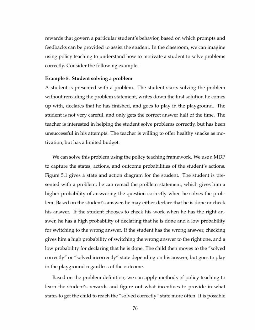
rewards that govern a particular student’s behavior, based on which prompts and

feedbacks can be provided to assist the student. In the classroom, we can imagine

using policy teaching to understand how to motivate a student to solve problems

correctly. Consider the following example:

Example 5. Student solving a problem

A student is presented with a problem. The student starts solving the problem

without rereading the problem statement, writes down the first solution he comes

up with, declares that he has finished, and goes to play in the playground. The

student is not very careful, and only gets the correct answer half of the time. The

teacher is interested in helping the student solve problems correctly, but has been

unsuccessful in his attempts. The teacher is willing to offer healthy snacks as mo-

tivation, but has a limited budget.

We can solve this problem using the policy teaching framework. We use a MDP

to capture the states, actions, and outcome probabilities of the student’s actions.

Figure 5.1 gives a state and action diagram for the student. The student is pre-

sented with a problem; he can reread the problem statement, which gives him a

higher probability of answering the question correctly when he solves the prob-

lem. Based on the student’s answer, he may either declare that he is done or check

his answer. If the student chooses to check his work when he has the right an-

swer, he has a high probability of declaring that he is done and a low probability

for switching to the wrong answer. If the student has the wrong answer, checking

gives him a high probability of switching the wrong answer to the right one, and a

low probability for declaring that he is done. The child then moves to the “solved

correctly” or “solved incorrectly” state depending on his answer, but goes to play

in the playground regardless of the outcome.

Based on the problem definition, we can apply methods of policy teaching to

learn the student’s rewards and figure out what incentives to provide in what

states to get the child to reach the “solved correctly” state more often. It is possible

76

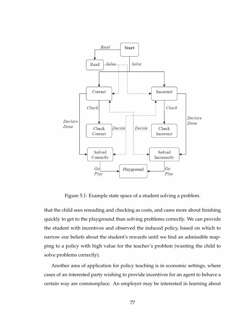
Figure 5.1: Example state space of a student solving a problem.

that the child sees rereading and checking as costs, and cares more about finishing

quickly to get to the playground than solving problems correctly. We can provide

the student with incentives and observed the induced policy, based on which to

narrow our beliefs about the student’s rewards until we find an admissible map-

ping to a policy with high value for the teacher’s problem (wanting the child to

solve problems correctly).

Another area of application for policy teaching is in economic settings, where

cases of an interested party wishing to provide incentives for an agent to behave a

certain way are commonplace. An employer may be interested in learning about

77

the preferences of an employee to figure out how to provide incentives for the

employee to perform well on the job. A search engine may be interested in learning

about the preferences of potential users, as to provide incentives for people to use

its service. A store may be interested in learning about the preferences of its users,

as to figure out how to provide incentives for users to buy products.

In each of these cases, the agent rewards may depend on many factors, some of

which are monetary but many of which are not. Furthermore, an agent may take

a number of actions before deciding to sign a contract or purchase a product, and

influencing earlier decisions could have important effects on the final outcome.

Policy teaching and its MDP framework can capture the dynamics of the process,

using observations of interrelated actions in complex domains to reason about the

agent’s preferences.

In addition to solving the policy teaching problem itself, the methods we have

developed may be useful for eliciting preferences in a complex domain and using

the preferences to accomplish a different task. For example, in user interface de-

sign, understanding the preferences of a user of a particular interface may provide

information about how to generate a better interface for that user. In policy teach-

ing, we are concerned with making an agent perform well taking the conditions

of the problem as given. In other cases, we may be interested in generating condi-

tions under which the agents preferences perform well. The elicitation methods we

have developed could be useful for learning agent preferences in these situations

as well.

5.1.2 Multi-agent Systems

Techniques from policy teaching may have applications to the study of multi-agent

systems, problems in which a social planner is interested in implementing an out-

come that depends on the inputs of self-interested agents whose preferences are

unknown to the social planner. This problem is well studied in the areas of mecha-

78

nism design and implementation theory, where the goal is to design a mechanism

that provide the rules of interactions under which the agents’ reports lead to the

desirable outcome.

In many situations, coming up with a mechanism with the desired properties is

a difficult task. This is especially true if the mechanism must work well regardless

of the true preferences of the agents. Furthermore, mechanisms may be difficult

to implement in practice. In domains with complex preferences, an agent may be

unable to express its preferences accurately to meet the mechanism’s demands.

Policy teaching provides an alternative method for implementing desirable

outcomes. Instead of designing the rules of interactions, we may be able to provide

minimal incentives to the agents to induce behaviors that lead to the implementa-

tion of desirable social outcomes. Instead of designing mechanisms that work well

regardless of the agents’ preferences, we may be able to learn the agents’ prefer-

ences by providing incentives and observing the induced behaviors of agents. We

can then provide incentives for these agents to behave as desired using a policy

teaching framework, or use the learned preferences to aid the design of a mecha-

nism for the agents in question.1

The single agent policy teaching framework we have introduced has natural ex-

tensions to multi-agent domains. Consider the following multi-agent policy teach-

ing problem.

Definition 22. Multi-agent policy teaching in domains with experts

An interested party is concerned with the policies of a group of n agents. Each

agent i faces a MDP M i = {Si, Ai, Ri, P i, γi}, and performs its optimal policy πi.

The interested party has knowledge of the agents’ MDPs, and can provide an ad-

missible incentive function ∆ such that agent i receives an incentive of ∆i(s) in

state s to modify the agent’s reward function to Ri + ∆i. Can the interested party

1The idea of using minimal incentives to implement outcomes has been previously consideredby Monderer and Tennenholtz [14]. Their work provided general results for normal form games,but do not deal with sequential decision tasks nor the issue of learning rewards.

79

find a ∆ to induce every agent i to perform policy πiE?

This problem requires the agent policies to be considered in unison, but is oth-

erwise no different than in the single agent case. We can write ∆ constraints over

all the agents, and map each agent i to an expert reward RiE that satisfies the IRL

constraints on the expert’s policy:

minRE

∑i

∑s

∆i(s) (5.1)

subject to:

∆i(s) = RiE(s)−Ri(s) ∀s, i (5.2)

(PiπiE−Pi

a)(I− γiPiπiE)−1Ri

E � ε ∀a ∈ A\a1, a1 ∈ π(s), i (5.3)∑i

∑s

∆i(s) ≤ Dmax (5.4)

∆i(s) ≥ 0 ∀s, i (5.5)

If the agents’ reward functions are unknown to the interested party, we can still

solve this problem by using a similar elicitation method as we use in the single

agent case. At each iteration, we can add IRL constraints on Ri to Program 5.1, and

use the linear program to find possible agents’ rewards that have mappings to the

set of expert policies.2 We can then provide ∆ to each of the agents, and observe

the induced policy. If every agent i performs the expert policy πiE , we can complete

the elicitation process with the mapping ∆. Otherwise, for the agents that did not

behave as expected, we can add IRL constraints on their induced policies. This

narrows the space of possible rewards for those agents. Since we are guaranteed

to make progress at every iteration, we will eventually be able to find a mapping

that induces each agent i to perform πiE , if such a mapping exists given the limits

on ∆.2We may also switch the objective (i.e. to maximizing the sum of the agents’ slacks), if we wish.

80

The multi-agent policy teaching problem in Definition 22 is simple, but can ap-

ply to many settings in which an interested party is concerned with the joint policy

of a group of agents. By framing the problem as one multi-agent policy teach-

ing problem instead of many single-agent policy teaching problems, the interested

party is able to find a way to distribute the incentives and find mappings that may

otherwise have not been admissible were the interested party to set aside limits on

the incentives provided to each agent. Further extensions of policy teaching to the

multi-agent domain provide an interesting area for future research.

5.2 Critique

In this section we acknowledge the major critiques of our work, and evaluate the

significance of these objections. We divide these critiques into five sections, and

propose extensions to the policy teaching framework to address the issues raised.

5.2.1 Parameters and Constraints

• The limits on ∆ do not accurately capture the amount of incentives the in-

terested party is willing to provide. Some states may be visited more than

once, and other states may not be visited at all.

One can capture the history of states visited by constructing a MDP that mod-

els history into the state space. This allows the interested party to specify in-

centives that can only be received once, such that an agent receiving an incen-

tive in a state will be transitioned to history states that take the information

into account to prevent the agent from receiving the incentive again. How-

ever, this requires an exponential blowup in the state space, and is only fea-

sible if the state space is small. Alternatively, we can introduce additional (or

different) constraints to reflect that a state may be visited forever in reasoning

about incentives. For example, we can constrain the total sum of discounted

incentives that an agent can receive by specifying ∆(s)/(1 − γ) < Dmax,∀s.

81

We can also construct a belief over what states the agent will visit and how

often, and tailor constraints on provided incentives based on learned beliefs.

In many cases, the admissible constraints on ∆ are sufficient. Many problems

can be modeled by a linear progression of states, where the transitions pre-

vent states from being revisited. Other problems have very few states that

can be revisited, and such states can be treated separately. In all problems

modeled, it is unlikely that an interested party desires the agent to perform a

policy in which an agent would be getting incentives over and over again. As

long as the policy teaching problem is solved, the limits on ∆ do accurately

reflect the incentives that the interested party provides. The exception to this

is goal states that the interested party wishes the agent to reach (i.e. “home”

in the child walking home example), but these cases can either be modeled

using absorbing states, or by taking into consideration that incentives pro-

vided in this state is for the discounted infinite future.

• The minimal slack ε needs to be set high for elicitation to finish quickly.

The amount of extra incentives that may be required for there be a map-

ping with ε slack is dependent on ε and the number of states n. If n is large,

a large ε may prevent available mappings. This forces a smaller ε to be set,

slowing the elicitation process.

This critique is a serious one, as it suggests that the length of elicitation can

increase quickly for larger state spaces not only because of the increase in the

space of possible rewards but due to the need to set a smaller ε. We can deal

with this issue in a number of ways. First, the amount of extra incentives

necessary for there to be a mapping is calculated in the worst case. There

is likely to be other mappings that do not require much extra incentive to be

provided for there to be a slack of ε. This suggests that we can greedily set ε to

be large, and scale back if necessary. Second, when the state space is large, we

may wish to assume some structure on the reward function, which can sig-

82

nificantly decrease the space of possible rewards that needs to be considered.

Finally, as we have shown in our experiments, our slack maximizing heuris-

tics allows our algorithm to scale well even for smaller ε. Improvements in

elicitation heuristics and ways to ensure progress other than the slack based

on ε can help to address this issue.

5.2.2 Assumptions

• Policy teaching assumes the interested party knows the agent’s MDP defi-

nition.

This assumption is not too restrictive. By watching the agent behave in the

domain, the interested party can learn the transition probability of an agent

moving from state to state based on his actions. The discount factor may

also be learned, possibly by observing the change in the agent’s responses to

provided incentives in different time periods.

• Policy teaching assumes that the interested party’s problem is based on the

same MDP−R definition as the agent.

We have framed the problem in this manner to give a sense of what the inter-

ested party is concerned with, but can represent the interested party’s pref-

erences generally as any function of the agent’s policy, independent of the

MDP−R definition.

• Policy teaching assumes the interested party knows his own reward G.

In cases where an interested party cannot write down his preferences, he may

still be able to specify policies that he is interested in the agent performing.

In such cases, we can have the agent attempt to map to these policies using

methods from policy teaching with an expert. In other cases, an interested

party may be able to specify his rewards roughly (either directly or through

elicitation), which can then be refined over time.

83

• Policy teaching assumes that the expert has the same MDP−R definition as

the agent.

We think of the expert as having a similar background as the agent, which

makes having the same (or similar) MDP−R definition likely. For example,

in the schooling setting, we think of the expert as a motivated student, not

a teacher whose problem definition may be very different. Furthermore, the

expert need not face the same MDPR

as the agent; if we are only concerned

with whether we can get the agent to perform like the expert, there need only

exist an admissible mapping to the expert’s policy.

• Policy teaching assumes that the interested party can observe the agent’s

behavior in every state. In some situations, actions may be unobservable

in certain states of interest.

An example of a scenario with unobservable action is when a service provider

is interested in increasing its customer base by learning the preferences of

people using competing services. If the service provider does not have ac-

cess to the behaviors of users of competing services (neither policies nor tra-

jectories), we cannot learn the rewards of these agents using policy teaching.

However, we may be able to infer these agents’ rewards in some other way in

order to apply policy teaching with known rewards. We can also use policy

teaching to learn the rewards of agents that are in the system, and use this

information to infer about how to motivate other users to switch providers.

While policy teaching does not deal with unobservable actions, its methods

may still be useful for these situations.

5.2.3 Expressiveness

• Rewards are placed on states, but in many cases it is more natural to ex-

press rewards on state-action pairs.

The current framework is easily extendable to reward functions over state-

84

action pairs. Furthermore, our elicitation algorithms do not rely on the form

of the reward function.

• Policy teaching is limited to finite state spaces.

We can represent infinite state spaces by assuming (or approximating) re-

ward functions as a linear combination of known features, where the weights

on these features represents the agent’s unknown reward function. Ng and

Russell [16] provided extensions to their IRL algorithms for infinite state

spaces, which we can apply to learn agent rewards given a policy. We can

find mappings to expert policies by providing incentives with ∆ constraints

based on the guessed weights and features. New evidence can then be incor-

porated in the same manner.

• Policy teaching requires the interested party to have access to the agent’s

policy. More realistically, the interested party may only see a set of actual

trajectories of the agent’s actions in the state space.

Ng and Russell [16] provides IRL algorithms for learning reward functions

based on trajectories. The extension is similar to IRL for infinite state spaces,

and can be incorporated into the policy teaching framework in much the

same way.

• Policy teaching does not incorporate priors over possible agent rewards.

Ramachandran and Amir [21] extended the IRL framework to Bayesian IRL

(BIRL), and presented algorithms for combining prior knowledge and ob-

servations to derive a probability distribution over the space of possible re-

wards. To allow for priors in policy teaching, we can use BIRL instead of IRL

to infer rewards. The distribution over possible rewards is useful for choos-

ing what to guess for the agent reward, and can lead to a shorter elicitation

process. In cases where the interest is in learning the true reward function,

Bayesian updating over possible rewards can also provide more detailed in-

formation about the agent’s preferences.

85

The prior-based preference elicitation literature on sequential decision tasks

may provide further ideas for how to use probabilistic distributions over

reward functions for policy teaching. Chajewska, Koller, and Parr [10] de-

veloped methods for finding queries that lead to the most information gain

based on a distribution over possible utility functions. Chajewska, Koller,

and Ormoneit [9] studied the problem of learning utility functions based on

prior probability distribution and observed behavior. Understanding how

these works fit within the policy teaching framework may be useful for pol-

icy teaching with priors.

5.2.4 The Elicitation Process

• Algorithms 1 and 2 complete without guessing the agent’s reward correctly.

These methods are useful for policy teaching, but not for learning the

agent’s rewards.

While our elicitation process may terminate before the true agent reward is

found, the process narrows the space of possible agent rewards. All rewards

that remain in the set of possible rewards “explains” the agent’s behaviors,

as they all satisfy the IRL constraints on the induced agent policies. Further

improvements are possible by incorporating a probability distribution over

rewards as we have described, but policy teaching as demonstrated does

plenty towards learning the agent’s true reward. An interesting open ques-

tion is whether we can use perturbations to the agent’s rewards to narrow

the space of possible rewards down to the agent’s true reward. One possi-

ble approach is to figure out policies other than the target policy to map the

agent’s reward, so as to be able to further narrow the space of rewards.

• The constraints on the agent’s reward are based on the values of the in-

centives provided. Values found this way do not reflect the agent’s true

reward. Also, the interested party may not be able to accurately map the

86

relation between different types of incentives.

We answer each part of the critique in turn. First, reward functions are map-

pings of preference relations; we are not interested in cardinal utility the-

ory here, and do not assign significance to the magnitude of the differences

between rewards. While we have been saying the agent’s “true” reward

throughout this work, we mean by this the reward function that expresses

the agent’s preferences with respect to the values used to represent the in-

centives. Any size comparisons we make in our discussion is with respect to

values assigned to the incentives. In domains where the incentives provided

are of the same form (i.e. all monetary), studies in economics provides tools

for modeling the relative values of different incentives.

In the case where different types of incentives are provided, we need to come

up with the relation between these types of incentives based on which to con-

strain the agent’s reward. If the relation we come up with is not the way that

the agent perceives the relationship, the constraints we add may not be very

meaningful in expressing the agent’s preference space. One possible solu-

tion is to treat the relationship as unknown and attempt to learn it. This can

be done outside of the policy teaching framework, or as part of the frame-

work where we consider one type of an incentive as an unknown function

of another. We can add constraints based on induced policies in the same

way, but with the incentive ∆ added expressed as a vector variable based on

the unknown function instead of a vector of values. We may also maintain

a probabilistic distribution over possible relation functions, and use obser-

vations and other evidence to update the distribution. Such solutions may

introduce additional computational complexity, and figuring out how to do

so generally but tractably is an interesting topic for future research.

• The policies the agent performs are assumed to be optimal for the agent’s

reward function. This may not be the case.

87

While policy teaching attempts to find a reward function that correspond to

the agent’s policies, the agent’s reward function may be changing over time.

Another possibly is that the agent’s rewards are constant, but the way he rea-

sons about them changes over time. Without a model how how the agent’s

reward evolves over time nor an accurate model of the agent’s reinforcement

learning process, placing IRL constraints on the agent’s reward may be too

restrictive. One possibly is to express the IRL constraints as soft constraints,

for which we wish to satisfy as closely as possible but allow for some con-

straints to be violated. Soft constraints on utility functions have proved to

be useful in preference elicitation for user interface generation [11, 12], and

could be useful for policy teaching as well.

5.2.5 Long Term Effects

• If the agent’s problem definition remains constant, the interested party

must provide incentives for the agent to behave as desired every time the

agent performs the sequential decision tasks.

In the teaching, parenting, and advertising examples that motivate our work,

we imagine that an interested party believes that the agent “absorbs” the

provided incentives over time, such that the agent will perform as the inter-

ested party desires without the interested party having to provide much (or

any) additional incentives in the future. This belief appears to be accurate

in many real-world situations, where an agent may form habits and stick to

his induced policy due to fixed costs for switching to another policy (possi-

bly the same fixed costs that kept the agent away from the policy desired by

the interested party in the first place). The interested party may also try to

gradually retract the amount of incentives provided, until he finds the mini-

mal incentive based on which the agent will still behave as desired. In other

cases, the interested party may be okay with providing incentives every time

88

the agent performs the tasks. For example, consider a consumer who only

buy products when they are on sale. A firm is happy to provide discounts

for the consumer every time as long as the firm can sell the good and make a

profit.

• Providing large incentives for an agent to perform as desired may have un-

desirable long term effects.

For large incentives, the agent may not be able to motivate himself enough to

internalize the incentives provided. Furthermore, large incentives may lead

to the agent performing as the interested party desires only because of the

incentives provided. For example, if a student wishes to solve problems cor-

rectly only because of the candy provided, the student may have no desire to

solve the problem correctly were the candy taken away. Just as the interested

party wishes for the incentives to be absorbed, the provided incentive may

dictate the agent’s behavior such that the agent’s inherent rewards wither

over time.

While this is not a direct critique of policy teaching but of the effect of in-

centives on people over time, it is an important issue that is worth studying

further. We may be able to model the long term effects of incentives, and take

such effects into consideration when providing incentives to agents. How-

ever, in many situations, the amount of incentives that can be provided is

limited, and only enough to motivate an agent towards decisions that he has

inherent values for. For example, we do not expect a firm to provide dis-

counts so large as to cause consumers to not make purchases unless steep

discounts were applied in the future. Nevertheless, understanding the dy-

namics of how an agent’s preferences and problem definition changes over

time can be valuable for policy teaching.

89

5.3 Open Questions and Future Research

In addition to potential applications and extensions, our work has created many

open questions for future research on the current policy teaching framework. They

include:

• Allowing for the provision of punishments. What effect does this have on

what policies can be induced? Does this allow for more effective elicita-

tion strategies? This may also be useful for extensions to multi-agent sys-

tems, where having punishments in addition to rewards allows for transfers

among agents.

• Improvements to objectives for choosing an agent reward. The effectiveness

of the objective determines whether the elicitation process can solve the pol-

icy teaching problem in a small number of rounds. Can we exploit the struc-

ture of certain domains, or incorporate prior information?

• Conduct more experiments on simulated and real-world examples. Evalu-

ate the effect of parameters on the length of the elicitation process. How

well do the current parameter setting methods perform? Attempt to better

understand why certain values work well (or poorly), and use found under-

standing to create better methods for parameter setting.

• Attempt to come up with more tractable formulations for policy teaching

without an expert. Can we find approximate solutions quickly?

• Generalize policy teaching with an expert. Instead of mapping to a specific

policy, how can we have the agent map to any policy within a set of policies?

90

Chapter 6

Conclusion

How can an interested party provide incentives to affect the behavior of an agent?

This question comes up in economics. This question comes up in education.

This question comes up in parenting. This question comes up whenever there is

a conflict of interest and one party wishes to affect the behavior of another party.

This question comes up in real-world examples, and in technical problems.

This is a hard problem to solve. It requires understanding how provided incen-

tives and inherent preferences are related to behavior. It requires understanding

how provided incentives and inherent agent preferences are related to each other.

It requires being able to model the agent’s behavior in complex domains. It re-

quires taking the limits on the incentives that the interested party can provide into

account. It requires knowledge of the preferences of the parties involved. When

preferences are unknown, solving the problem requires learning the preferences.

This thesis developed a general framework for studying this problem that takes

these requirements into account.

6.1 Brief Review

In Chapter 1, we introduced real-world scenarios in which an interested party

wishes to affect the behavior of an agent by providing incentives. We outlined the

91

major obstacles that the interested party faces in trying to get an agent to behave as

desired, and provided a non-formal definition of the policy teaching problem. We

described our contributions for studying the problem in a Markov Decision Pro-

cess (MDP) framework, and discussed our work in the context of related works in

contract theory, apprenticeship learning, and preference elicitation.

In Chapter 2, we motivated and developed the MDP formalism for modeling

sequential decision tasks. We used the framework to provide a formal definition

of the policy teaching problem with known rewards. We studied the problem in

domains without an expert, and formulated a mixed integer program as a solution

to a difficult technical problem. We then considered the policy teaching problem

in domains with an expert, where our solution is a simple linear program.

In Chapter 3, we introduced techniques of inverse reinforcement learning (IRL)

for finding the space of reward functions to corresponds to a policy. We used IRL

to generalize our solution for domains with an expert, both to allow for more po-

tential mappings and domains where the agent’s reward is known but the expert’s

reward is unknown. We then introduced the policy teaching problem with un-

known agent rewards, and realized that while IRL provided an useful starting

point, we required additional evidence about the agent’s reward to solve the pol-

icy teaching problem. We discussed why direct utility elicitation methods may not

apply well to policy teaching, and proposed a method for generating additional

evidence about the agent’s rewards based on observations of the agent’s responses

to provided incentives. We turned this method into an elicitation algorithm for

policy teaching in domains with an expert, and proved bounds on the number

of elicitation rounds the algorithm requires before returning a solution. We ex-

tended the ideas to domains without an expert, constructed a similar algorithm

for such domains, and proved similar bounds on the number of elicitation rounds.

Having presented general elicitation algorithms for policy teaching with unknown

reward, we discussed possible objective functions for the elicitation process, and

92

introduced tractable heuristics for reducing the number of elicitation rounds in

practice.

In Chapter 4, we discussed experiments on using our algorithms with the heuris-

tics we had introduced. We described methods for setting the various parameters

of the algorithms which may allow for a shorter elicitation process. We presented

results on a motivating example, and showed that we can complete the elicitation

process in a small number of rounds for both domains with and without an ex-

pert. For the domain with an expert, we studied the effects of setting parameters,

and determined that while our set parameters performed well, improvements are

possible. For the domain without an expert, we saw that while we were able to

find a solution to the policy teaching problem for our example, the computational

complexities introduced by the mixed integer programs may become a bottleneck

for larger domains.

In Chapter 5, we discussed the potential applications of our work, both for

real-world settings and for multi-agent system design. We presented the major cri-

tiques of our work, which we divided into sections on parameters and constraints,

assumptions, expressiveness, elicitation process, and long term effects. We pro-

posed extensions to address these critiques, and concluded the chapter with open

questions on the policy teaching framework for future research.

6.2 Conclusion

Our work provides a general framework for studying the policy teaching prob-

lem. The policy teaching algorithms we have introduced provide a new way for

eliciting preferences that draws from the connection among behaviors, provided

incentives, and inherent preferences. Our policy teaching framework provides a

solid foundation for possible extensions and applications, and offers exciting open

questions for future research.

93

References

[1] Peter Abbeel and Andrew Y. Ng. Apprenticeship learning via inverse rein-

forcement learning. In Proceedings of the Twenty-first International Conference on

Machine Learning, 2004.

[2] Joseph Beck, Mia Stern, and Erik Haugsjaa. Applications of AI in education.

Crossroads, 3(1):11–15, 1996.

[3] Jennifer Boger, Pascal Poupart, Jesse Hoey, Craig Boutilier, Geoff Fernie, and

Alex Mihailadis. A Planning System Based on Markov Decision Processes

to Guide People with Dementia Through Activities of Daily Living. IEEE

Transactions on Information Technology in Biomedicine, 10(2):323–333, 2006.

[4] Patrick Bolton and Mathias Dewatripont. Contract Theory. MIT Press, 2005.

[5] Craig Boutilier. POMDP Formulation of Preference Elicitation Problems. In

Proceedings of the Eighteenth National Conference on Artificial Intelligence, pp.

239–246, 2002.

[6] Craig Boutilier, Relu Patrascu, Pascal Poupart, and Dale Schuurmans.

Constraint-based Optimization with the Minimax Decision Criterion. Ninth

International Conference on Principles and Practice of Constraint Programming, pp.

168–182, 2003.

[7] Craig Boutilier, Relu Patrascu, Pascal Poupart, and Dale Schuurmans. Regret-

based Utility Elicitation in Constraint-based Decision Problems. In Proceedings

94

of the Nineteenth International Joint Conference on Artificial Intelligence, pp. 929–

934, 2005.

[8] Craig Boutilier, Tuomas Sandholm, and Rob Shields. Eliciting Bid Taker Non-

price Preferences in (Combinatorial) Auctions. In Proceedings of the Nineteenth

National Conference on Artificial Intelligence, pp. 204–211, 2004.

[9] Urszula Chajewska, Daphne Koller, and Dirk Ormoneit. Learning an Agent’s

Utility Function by Observing Behavior. In Proceedings of the Eighteenth Inter-

national Conference on Machine Learning, 2001.

[10] Urszula Chajewska, Daphne Koller, and Ronald Parr. Making Rational De-

cisions using Adaptive Utility Elicitation. In Proceedings of the 17th National

Conference on Artificial Intelligence, pp. 363–369, 2000.

[11] Krzysztof Z. Gajos, Jing Jing Long, and Daniel S. Weld. Automatically Gener-

ating Custom User Interfaces for Users with Physical Disabilities. In Proceed-

ings of the Eight International ACM SIGACCESS Conference on Computers and

Accessibility, pp. 243–244, 2006.

[12] Krzysztof Z. Gajos and Daniel S. Weld. Preference Elicitation for Interface

Optimization. In Proceedings of the eighteenth annual ACM symposium on User

interface software and technology, pp. 173–182, 2005.

[13] Jean-Jacques Laffront and David Martimort. The Theory of Incentives: The

Principal-Agent Model. Princeton University Press, 2001.

[14] Dov Monderer and Moshe Tennenholtz. k-Implementation. In Proceedings of

the fourth ACM conference on Electronic Commerce, pp. 19–28, 2003.

[15] Andrew Y. Ng, Daishi Harada, and Stuart Russell. Policy invariance under

reward transformations: Theory and application to reward shaping. In Pro-

ceedings of the Sixteenth International Conference on Machine Learning, 1999.

95

[16] Andrew Y. Ng and Stuart Russell. Algorithms for inverse reinforcement learn-

ing. In Proceedings of the Seventeenth International Conference on Machine Learn-

ing, 2000.

[17] Relu Patrascu, Craig Boutilier, Rajarshi Das, Jeffrey O. Kephart, Gerald

Tesauro, and William E. Walsh. New Approaches to Optimization and Utility

Elicitation in Autonomic Computing. In Proceedings of the Twentieth national

Conference on Artificial Intelligence, pp. 140–145, 2005.

[18] Bob Price and Craig Boutilier. A Bayesian Approach to Imitation in Reinforce-

ment Learning. In Proceedings of the Eighteenth International Joint Conference on

Artificial Intelligence, pp. 712–717, 2003.

[19] Bob Price and Craig Boutilier. Accelerating Reinforcement Learning through

Implicit Imitation. Journal of Artificial Intelligence Research, 19:569–629, 2003.

[20] Martin L. Puterman. Markov Decision Processes: Discrete Stochastic Dynamic

Programming. John Wiley & Sons, New York, NY, 1994.

[21] Deepak Ramachandran and Eyal Amir. Bayesian Inverse Reinforcement

Learning. Twentieth International Joint Conference on Artificial Intelligence, 2007.

[22] Tuomas Sandholm and Craig Boutilier. Preference Elicitation in Combinato-

rial Auctions. Combinatorial Auctions, Chapter 10. MIT Press, 2006.

[23] Aaron P. Shon, David B. Grimes, Chris L. Baker, and Rajesh P.N. Rao. A Prob-

abilistic Framework for Model-Based Imitation Learning. In Proceedings of

CogSci, 2004.

[24] Hal R. Varian. Revealed Preference. Samuelsonian Economics and the Twenty-

First Century, Chapter 5. Oxford University Press, 2007.

96

[25] Tianhan Wang and Craig Boutilier. Incremental Utility Elicitation with the

Minimax Regret Decision Criterion. In Proceedings of the Eighteenth Interna-

tional Joint Conference on Artificial Intelligence, pp. 309–316, 2003.

97