Policy Search For Learning Robot Control Using Sparse Data

B. Bischoff1, D. Nguyen-Tuong1, H. van Hoof2, A. McHutchon3,C. E. Rasmussen3, A. Knoll4, J. Peters2,5, M. P. Deisenroth6,2

Abstract— In many complex robot applications, such asgrasping and manipulation, it is difficult to program desiredtask solutions beforehand, as robots are within an uncertainand dynamic environment. In such cases, learning tasks fromexperience can be a useful alternative. To obtain a soundlearning and generalization performance, machine learning,especially, reinforcement learning, usually requires sufficientdata. However, in cases where only little data is availablefor learning, due to system constraints and practical issues,reinforcement learning can act suboptimally. In this paper, weinvestigate how model-based reinforcement learning, in partic-ular the probabilistic inference for learning control method(PILCO), can be tailored to cope with the case of sparse datato speed up learning. The basic idea is to include further priorknowledge into the learning process. As PILCO is built on theprobabilistic Gaussian processes framework, additional systemknowledge can be incorporated by defining appropriate priordistributions, e.g. a linear mean Gaussian prior. The resultingPILCO formulation remains in closed form and analyticallytractable. The proposed approach is evaluated in simulationas well as on a physical robot, the Festo Robotino XT. Forthe robot evaluation, we employ the approach for learning anobject pick-up task. The results show that by including priorknowledge, policy learning can be sped up in presence of sparsedata.

I. INTRODUCTION

In recent years, robots have increasingly become a naturalpart of daily life. As service robots, they are introduced to thecustomer market fulfilling tasks, such as lawn mowing andvacuum cleaning. However, most of today’s robot applicationsare rather simple, where the tasks are pre-programmed. Morecomplex applications, such as grasping and manipulation,are difficult to hard-code beforehand. The main reasonis that robots and other autonomous systems are withinuncertain, stochastic and dynamic environments, which cannot be analytically and explicitly described, making pre-programming impossible in many cases. Here, machinelearning offers a powerful alternative.

Especially for robot control manual development of controlstrategies can be challenging. It is often hard to accuratelymodel the uncertain and dynamic environment while inferringappropriate controllers for solving desired tasks. In such

1Cognitive Systems, Bosch Corporate Research, Germany2Intelligent Autonomous Systems, TU Darmstadt, Germany3Computational and Biological Learning Lab, Univ. of Cambridge, UK4Robotics and Embedded Systems, TU München, Germany5Max Planck Institute for Intelligent Systems, Tübingen, Germany6Department of Computing, Imperial College London, UKThe research leading to these results has received funding from the

European Community’s Seventh Framework Programme (FP7/2007-2013)under grant agreement #270327 and the Department of Computing, ImperialCollege London.

cases, reinforcement learning (RL) can help to efficientlylearn a control policy from sampled data instead of manualdesign using expert knowledge [1], [4], [5]. State-of-the-art RL approaches, e.g. policy search techniques [3], usuallyrequire sufficiently many data samples for learning an accuratedynamics model, based on which the control policy can beinferred. Thus, in the presence of sparse data RL approachescan be suboptimal, especially, for high-dimensional learningproblems. In this paper, we investigate how model-basedpolicy search, in particular the probabilistic inference forlearning control method (PILCO), can be tailored to copewith sparse training data to speed up the learning process.

The policy search RL algorithm PILCO [2] employsGaussian processes (GP) to model the system dynamics.PILCO has been shown to be effective for learning control inan uncertain and dynamic environment [12], [13]. To furtherspeed up learning and to make PILCO appropriate for learningwith sparse data in high-dimensional problems, e.g. an 18dimensional dynamics model, we propose to include furtherprior knowledge into the learning process. As non-parametricGP regression is employed as the core technique in PILCO,prior knowledge can be straightforwardly incorporated bydefining appropriate prior distributions. It has been shown inthe past that incorporating prior knowledge into GP learningcan significantly improve the learning performance in thepresence of sparse data [11]. In this study, we choose alinear mean Gaussian distribution as prior for modeling thesystem dynamics. This prior is especially appropriate forsystems with underlying linear or close to linear behavior.The evaluations show that this choice of prior can help toimprove the learning performance while the resulting RLformulation remains in closed form and analytically tractable.

The remainder of the paper will be organized as follows.First, we give a brief review on the basic concepts of RL andPILCO. In Section II, we introduce the extension of PILCOwhere a linear mean Gaussian prior is employed. In SectionIII, we provide experiments in simulation as well as on aphysical robot. Here, we aim to learn an object pick-up taskwith the Festo Robotino XT shown in Figure 1, using theproposed approach. A conclusion and summary can be foundin Section IV.

A. Background: Reinforcement Learning

RL considers a learning agent and its interactions with theenvironment [3], [7]. In each state s ∈ S the agent can applyan action a ∈ A and, subsequently, moves to a new states′. The system dynamics define the next state probabilityp(s′|s, a). In every state, the agent determines the action to

2014 IEEE International Conference on Robotics & Automation (ICRA)Hong Kong Convention and Exhibition CenterMay 31 - June 7, 2014. Hong Kong, China

978-1-4799-3685-4/14/$31.00 ©2014 IEEE 3882

Fig. 1: The Festo Robotino XT, a mobile service robot witha pneumatic arm, used for evaluation.

be used according to its controller, π : S → A. Applicationof the controller for T timesteps results in a state-actiontrajectory {s0, a0}, {s1, a1}, . . . , {sT−1, aT−1}, sT denotedas rollout. Multiple rollouts will not be identical in case ofuncertainty and noise. Thus, probability distributions need tobe employed to describe the controller rollout. Each state siis rated by the environment with a cost function, c : S → R.It is the goal of the learning agent to find a controller thatminimizes the expected long-term cost J(π) given by

J(π) =

T∑t=0

Est [c(st)] (1)

where st is the resulting state distribution when the controllerπ is applied for t timesteps. The cost function c encodesthe learning goal and must be set accordingly. The learningalgorithm uses samples si, ai, si+1 to optimize the controllerwith respect to the expected long-term cost. The way howthis experience is used to learn a new, improved controller πis what makes the difference between various RL approaches.For example, RL techniques can be classified as model-freeand model-based. While model-free RL directly optimizesthe controller π, model-based approaches explicitly model thedynamics, i.e. p(s′|s, a), and optimize the controller usingthis model. Another characterization of RL methods is policysearch versus value-function approaches. In policy search, thelearning algorithm directly operates on the parameters θ of acontroller πθ to minimize the expected long-term cost. Onthe other hand, value-function approaches learn a long-termcost estimate for each state. Using this estimate, a controllercan be determined.

B. PILCO: A Fast Policy Search Approach

To find control parameters θ∗, which minimize Eq. (1),we employ the PILCO policy search framework [2] tolearn low-level controllers. PILCO’s key component is aprobabilistic model of the robot’s forward dynamics p(s′|s, a),implemented as a Gaussian process (GP) [6].

Policy learning consists of two steps: policy evaluationand policy improvement. For policy evaluation, we use theGP dynamics model to iteratively compute Gaussian approx-imations to the long-term predictions p(s0|θ), . . . , p(sT |θ)

for a given policy parametrization θ. Since PILCO explicitlyaccounts for model uncertainty in this process, it reduces theeffect of model bias [2]. With the predicted state distributionsp(st|θ), t = 1, . . . , T , an approximation to the expected long-term cost J(π) in Eq. (1) and the gradients dJ(θ)/dθ canbe computed analytically. For policy improvement, we usethis gradient information and apply Quasi-Newton methodsfor non-convex optimization to find the desired set of policyparameters θ∗. Note that policy learning does not involve anyinteractions with the robot, but is solely based on the learnedGP dynamics model.

When the policy parameters have been learned, the cor-responding policy is applied to the robot. The data fromthis experiment is collected and used to update the learneddynamics model. Then, this new model is used to updatethe policy. The process of model learning, policy learning,and application of the policy to the robot is repeated untila good policy is found. In this framework, it is essentialto obtain a sufficiently accurate dynamics model. If onlylittle data is available, e.g. 200 data points for an 18 dim.model, the model learning performance can be improvedwhen using additional prior system knowledge [11]. As ourconsidered problems appear to have a linear underlying trend,we choose a linear mean prior for the GP employed forlearning the forward dynamics. By doing so, the resultingPILCO formulation remains in closed form as shown in thefollowing section.

II. PILCO WITH LINEAR MEAN GAUSSIAN PRIOR

At the heart of the PILCO algorithm lies the Gaussianprocess dynamics model. GPs provide a principled andpowerful method for modelling observed data by specifyinga distribution over possible function values h(x), i.e.

h(x) ∼ GP(m(x), k(x, x′)) (2)

where m(x) is the mean function and k(x,x′) is thecovariance function. For a given data set {X,y}, a GPprediction at a test point x∗ is normally distributed with

h∗ ∼ N (µ∗, Σ∗) , (3)

µ∗ = k(x∗, X)[K + σ2nI]−1 (y −m(X)) +m(x∗) ,

(4)

, k(x∗, X)β +m(x∗) , (5)

Σ∗ = k(x∗,x∗)− k(x∗, X)[K + σ2nI]−1 k(X,x∗) (6)

where K = k(X,X), β = [K + σ2nI]−1 (y−m(X)), σ2

n isa noise variance parameter. Within the GP framework, theGP hyperparameters including the parameters of the meanfunction m(x) can be estimated from data [6]. In case ofmultiple output dimensions, a separate GP can be trained foreach output dimension.

In previous applications of PILCO, the default prior meanfunction m(x) has been set to either zero, m(x) = 0,or the identity function m(x) = x [2]. Many systems ofinterest, however, contain a number of underlying linear, orclose to linear, relationships. This is especially true for statespaces containing both variables and their time derivatives

3883

(e.g. positions and velocities) for which a linear relationship(Euler integration) can be a good starting point. By using amore informative linear mean prior, the GP can model thecomplex nonlinearities better and has improved extrapolationperformance. Using a linear mean prior with the GP dynamicsmodel therefore promises performance improvements overprevious work. The PILCO algorithm makes predictionsusing its dynamics model at uncertain test points. In thissection, we derive the necessary predictive equations for aGP with a affine mean prior, m(x) = Ax+ b, when the testpoints are uncertain, i.e. x∗ ∼ N (µ,Σ). For computationaltractability, we choose the squared-exponential covariancefunction, k(x,x′) = α2 exp(− 1

2 (x−x′)TΛ−1(x−x′)), withhyperparameters α2 (signal variance) and Λ (squared lengthscales), which are learned within the GP framework.

For an uncertain test input x∗ ∼ N (µ,Σ), the predictivemean µ∗ is given by

µ∗ = Ex∗,h[h(x∗)] = Ex∗ [Eh[h(x∗)]]

= Ex∗ [k(x∗, X)β +m(x∗)] = βTq +Aµ+ b , (7)

where qi = η exp(− 1

2 (xi − µ)T (Σ + Λ)−1(xi − µ))

with η = α2∣∣ΣΛ−1 + I

∣∣−1/2. The predictive variancevarx∗,h[h(x∗)] is given as

varx∗,h[h(x∗)] = Ex∗ [varh[h(x∗)]] + Ex∗

[Eh[h(x∗)]

2]

− Ex∗ [Eh[h(x∗)]]2. (8)

Since varh[h(x∗)] does not depend on the prior mean function,we use the derivation from [9]. Thus,

Ex∗ [varh[h(x∗)] = α2 − tr(

(K + σ2ε I)−1Q̃

), (9)

Q̃ = Ex∗ [k(X,x∗)k(x∗, X)] , (10)

Q̃i,j =∣∣2ΣΛ−1 + I

∣∣−1/2 k(xi,µ)k(xj ,µ)

exp(

(zi,j − µ)T (

Σ + 12Λ)−1

ΣΛ−1 (zi,j − µ)),

and zi,j =xi+xj

2 . Using Eq. (7) we get

Ex∗ [Eh[h(x∗)]]2

= (Aµ+ b+ βTq)2 (11)

which leaves

Ex∗

[Eh[h(x∗)]

2]

= Ex∗ [(k(x∗, X)β)2 +m(x∗)2

+ 2m(x∗)k(x∗, X)β]. (12)

We derive the expected values on the right hand side ofEq. (12) in a form generalized to multiple output dimensions,since we will reuse the equations for calculating the covari-ance between output dimensions. Here, the superscripts u, vdenote the respective output dimensions. From Eq. (10), weobtain

Ex∗ [k(x∗, X)βuk(x∗, X)βv] = (βu)T Q̃βv , (13)

Ex∗ [mu(x∗)mv(x∗)] = Au Ex∗ [x∗x

T∗ ](Av)T

+ buAvµ+ bvAuµ+ bubv

= Au(Σ + µµT

)(Av)T+

buAvµ+ bvAuµ+ bubv . (14)

The final expectation is

Ex∗ [mu(x∗)kv(xi,x∗)]

= Au Ex∗ [x∗kv(xi,x∗)] + bu Ex∗ [kv(xi,x∗)]

= Akα2v(2π)D/2|Λv|1/2

·∫x∗N (x∗|xi,Λv)N (x∗|µ,Σ)dx∗ + buqvi

= Auqvi cvi + buqvi (15)

with

ci = Λ(Σ + Λ)−1µ+ Σ(Σ + Λ)−1xi .

Here, we exploited the fact that the squared-exponential kernelcan be written as an unnormalized Gaussian distribution.Using the relationship given in Eq. (8), we can now combineequations (9)–(15), for a single output dimension to get

varx∗,h[h(x∗)] = α2 − tr(

(K + σ2ε I)−1Q̃

)+ βQ̃βT

− (βT q)2 +AΣAT − 2AµβT q

+ 2A

n∑i=1

βiqici

for the predictive variance. For each output dimension hu(x),we independently train a GP and calculate the mean andvariance of the predictive Gaussian distribution as derivedabove. Next, we consider the predictive covariance betweenoutput dimensions u 6= v. As a first step, we can write

covx∗,h[hu(x∗), hv(x∗)] = Ex∗ [covh[hu(x∗), h

v(x∗)]]

+ covx∗ [Eh[hu(x∗)],Eh[hv(x∗)]] . (16)

Due to the conditional independence assumption, i.e.hu(x∗) ⊥⊥ hv(x∗) | x∗, the first term in Eq. (16) is zero,which leaves the covariance of the means. This can be solvedanalogously to eq. (12) and (13) to get

covh,x∗ [hu(x∗), hv(x∗)]

= (βu)TQβv − (βu)Tqu(βv)Tqv +AuΣ(Av)T

+Aun∑i=1

βvi qvi cvi +Av

n∑i=1

βui qui c

ui

−Auµ(βv)Tqv −Avµ(βu)Tqu

for the covariance between output dimensions. Finally, weproceed to derive the input-output covariance between theinput x∗ ∼ N (µ,Σ) and the estimated function outputh(x∗) ∼ N (µ∗,Σ∗). We need this covariance Σx∗,h∗ toderive the joint distribution

p(x∗, h(x∗)) = N([µµ∗

],

[Σ Σx∗,h∗

ΣTx∗,h∗Σ∗

])of the function input x∗ ∼ N (µ,Σ) and output h(x∗). It is

Σx∗,h∗ = Ex∗,h

[x∗h(x∗)

T]− Ex∗ [x∗] Ex∗,h [h(x∗)]

T,

where the second term is directly given by Eq. (7). To computeEx∗,h

[x∗h(x∗)

T], we first rewrite the expression

Ex∗,h

[x∗h(x∗)

T]

= Ex∗ [x∗m(x∗) + x∗k(x∗, X)β]

= Ex∗

[x∗x

T∗]AT + bµ+ Ex∗ [x∗k(x∗, X)β] .

3884

Now, we use again the definition of the variance, Eq. (15) andthe simplification steps described in [14, eq. (2.68)–(2.70)]to obtain

Σx∗,h∗ =

n∑i=1

βiqiΣ(Σ + Λ)−1(xi − µ) + ΣAT

for the input-output covariance. This concludes the derivationsfor the GP prediction with a linear prior mean function atuncertain test inputs.

Note that all terms for the prediction with linear meanprior can be split in the terms we have in the zero meancase, plus some additional expressions. Using PILCO withlinear mean prior, the complexity to compute the additionalterms for the mean and input-output covariance is O (DE)resp. O

(D2E

)and, hence, independent of the number of

training samples n. Here, D denotes the input dimensionality(i.e. state plus action dimensionality) while E corresponds tothe number of output dimensions (i.e. state dimensionality).Assuming n > D,E, variance and covariance prediction canbe performed in O

(DE2 + nD2

), where n is the number

of training samples. Compared to O(DE2n2

)for the zero

prior mean prediction (see [14]), the additional terms for thelinear mean prior do not increase the complexity class.

III. EXPERIMENTS & EVALUATIONS

In this section, we evaluate the proposed approach forlearning control policies in the sparse data setting. First,we apply our extended PILCO algorithm on a control taskin simulation, namely position control of a throttle valve.Subsequently, we learn an object grasping policy for a pick-up task with the Festo Robotino XT, a mobile service robotwith pneumatic arm shown in Figure 1. In both cases, sparsedata is employed for learning the system dynamics, e.g. 75sampled data points for learning throttle valve control and200 data points for learning pick-up task.

A. Comparative Evaluation on a Throttle Valve Simulation

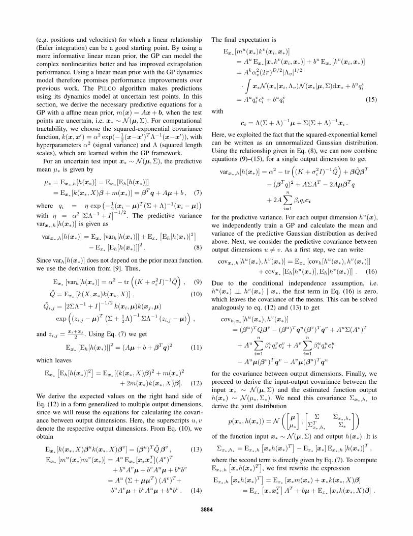
Fig. 3: Throttle valvesystem to regulate a gasor fluid flow.

The throttle valve shown inFigure 3 is an important technicaldevice that allows flow regulationof gas and fluids. It is widely usedin various industrial applications,such as cooling systems for powerplants and pressure control ingasoline combustion engines. Thevalve system basically consists ofa DC-motor, a spring and a valvewith position sensors. The dynam-ics of the throttle valve systemcan be analytically approximatedby the model[α̇(t)ω̇(t)

]=

[0 1−Ks −Kd

] [α(t)ω(t)

]+

[0

L(t)

]+

[0

T (t)

], (17)

where α and ω are the valve angle and corresponding angularvelocity T is the actuator input and L(t) = Cs−Kf sgn(ω(t))[8]. The parameters Ks, Kd, Kf and Cs are dynamicsparameters and need to be identified for a given system. Here,

we use Ks = 1.5, Kd = 3, Kf = 6, Cs = 20. The input T isdetermined as T (t) = u(t)Kj/(R), where u(t) ∈ [−20, 20]is the input voltage with Kj = 50 and R = 4.

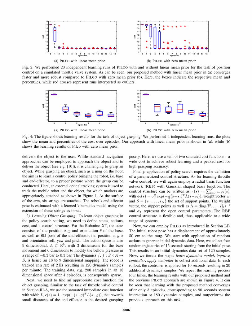
In the RL setting, we describe the system state as valveangle α and velocity ω, the voltage u(t) corresponds to theaction space. The learning goal is to move the valve to adesired angle g. Hence, the cost function can be defined assaturated immediate cost c(s) = 1−exp(−(s−g)TL(s−g))with diagonal width matrix L [2]. We set the start stateto be α0 = 10◦, the desired angle is g = 90◦. In eachcontroller rollout, 15 dynamics samples s, a, s′ are collected.This results in a sparse data set of 75 samples after initialrandom movements and 4 learning episodes. The controllerstructure employed for policy search is a radial basis function(RBF) network, which will be described in Section III-B inmore detail. Figure 2 shows the learning results of PILCOwith and without usage of a linear mean Gaussian prior, asintroduced in last section. As can be seen from the results,the proposed approach using a linear mean prior convergesfaster and more robustly in this control task.

B. Learning a Pick-Up Task with a Festo Robotino XT

In this section, we aim to solve an object pick-up taskusing the proposed method. Here, a mobile robot, namelya Festo Robotino XT shown in Figure 1, is controlled toapproach the target object, e.g. a mug, to grasp this objectand, subsequently, deliver it to the user. In the next sections,we describe the Festo Robotino XT and the pick-up task first.In Section III-B.2, learning results of the task are providedand discussed in detail.

1) Object Grasping with Robotino: The Festo RobotinoXT shown in Figure 1, is a mobile service robot with anomni-directional drive and an attached pneumatic arm. Thedesign of the arm is inspired biologically by the trunk of anelephant. The arm itself consists of two segments with threebellows each. The pressure in each bellow can be regulatedin a range of 0.0 to 1.5 bar to move the arm. As material, apolyamide structure is employed resulting in a low arm weight.A soft gripper is mounted as end-effector implementing theso-called Fin-Ray-effect. Under pressure at a surface point,the gripper does not deviate but bends towards that point and,thus, allows a form-closed and stable grasp.

The robot is also well-suited to operate in human environ-ments, as the low pressure pneumatics allows a compliantbehavior. However, kinematics and dynamics of the pneumaticarm are quite complex. A further constraint of the Robotinois the limited work space of the arm. Due to this limitedworkspace, we need to control the robot base as well as thearm movement while grasping an object. Thus, the forwarddynamics for the grasping control results in an 18 dimensionalmodel. These dimensions correspond to the robot state, i.e.position and orientation of the base and end-effector, androbot action space, i.e. base movements and change in armpressures.

The application we consider for the Robotino are pick-uptasks. This task can be partitioned into three phases: the robotapproaches the object, grasps the object and, subsequently,

3885

0 1 2 3 4 5 6 7 8 9 10 11 12 13 14 157

8

9

10

11

12

13

14

15

16

episodes

cost

(a) PILCO with linear mean prior

0 1 2 3 4 5 6 7 8 9 10 11 12 13 14 157

8

9

10

11

12

13

14

15

16

episodes

cost

(b) PILCO with zero mean prior

Fig. 2: We performed 20 independent learning runs of PILCO with and without linear mean prior for the task of positioncontrol on a simulated throttle valve system. As can be seen, our proposed method with linear mean prior in (a) convergesfaster and more robust compared to PILCO with zero mean prior (b). Here, the boxes indicate the respective mean andpercentiles, while red crosses represent runs interpreted as outliers.

0 1 2 3 4 5

4

6

8

10

12

14

16

18

20

22

episodes

cost

(a) PILCO with linear mean prior

0 1 2 3 4 5

4

6

8

10

12

14

16

18

20

22

episodes

cost

(b) PILCO with zero mean prior

Fig. 4: The figure shows learning results for the task of object grasping. We performed 4 independent learning runs, the plotsshow the mean and percentiles of the cost over episodes. Our approach with linear mean prior is shown in (a), while (b)shows the learning results of Pilco with zero mean prior.

delivers the object to the user. While standard navigationapproaches can be employed to approach the object and todeliver the object (see e.g. [10]), it is challenging to grasp anobject. While grasping an object, such as a mug on the floor,the aim is to learn a control policy bringing the robot, i.e. baseand end-effector, to a proper posture where the grasp can beconducted. Here, an external optical tracking system is used totrack the mobile robot and the object, for which markers areappropriately attached as shown in Figure 1. At the surfaceof the arm, six strings are attached. The robot’s end-effectorpose is estimated with a learned kinematics model using theextension of these strings as input.

2) Learning Object Grasping: To learn object grasping inthe policy search setting, we need to define states, actions,cost, and a control structure. For the Robotino XT, the stateconsists of the position x, y and orientation θ of the base,as well as 6D pose of the end-effector, i.e. position x, y, zand orientation roll, yaw and pitch. The action space is also9 dimensional, A ⊂ R9, with 3 dimensions for the basemovement and 6 dimensions to modify the bellow pressure ina range of −0.3 bar to 0.3 bar. The dynamics f , f : S×A→S, is hence an 18 to 9 dimensional mapping. The robot istracked at a rate of 2 Hz resulting in 120 dynamics samplesper minute. The training data, e.g. 200 samples in an 18dimensional space after 4 episodes, is consequently sparse.

Next, we need to find an appropriate cost function forobject grasping. Similar to the task of throttle valve controlin Section III-A, we use the saturated immediate cost functionwith width L, c(s) = 1−exp(−(s−g)TL(s−g)), that rewardssmall distances of the end-effector to the desired grasping

pose g. Here, we use a sum of two saturated cost functions—awide cost to achieve robust learning and a peaked cost forhigh grasping accuracy.

Finally, application of policy search requires the definitionof a parametrized control structure. As for learning throttlevalve control, we will again employ a radial basis functionnetwork (RBF) with Gaussian shaped basis function. Thecontrol structure can be written as π(s) =

∑Ni=0 wiφi(s),

with φi(s) = σ2f exp(− 1

2 (s−si)TΛ(s−si)), weight vector w,and S = {s0, . . . , sN} the set of support points. The weightvector, the support points as well as Λ = diag(l21, . . . , l

2D)−1

and σf represent the open control parameters. The RBFcontrol structure is flexible and, thus, applicable to a widerange of systems.

Now, we can employ PILCO as introduced in Section I-B.The initial robot pose has a displacement of approximately50 cm to the mug. We start with application of randomactions to generate initial dynamics data. Here, we collect fourrandom trajectories of 15 seconds starting from the initial pose.This results in an initial dynamics data set of 120 samples.Now, we iterate the steps: learn dynamics model, improvecontroller, apply controller to collect additional data. In eachrollout, the controller is applied for 10 seconds resulting in 20additional dynamics samples. We repeat the learning processfour times, the learning results with our proposed method andthe previous PILCO approach are shown in Figure 4. It canbe seen that learning with the proposed method convergesafter only 3 episodes, corresponding to 90 seconds systeminteraction or 180 dynamics samples, and outperforms theprevious approach on this task.

3886

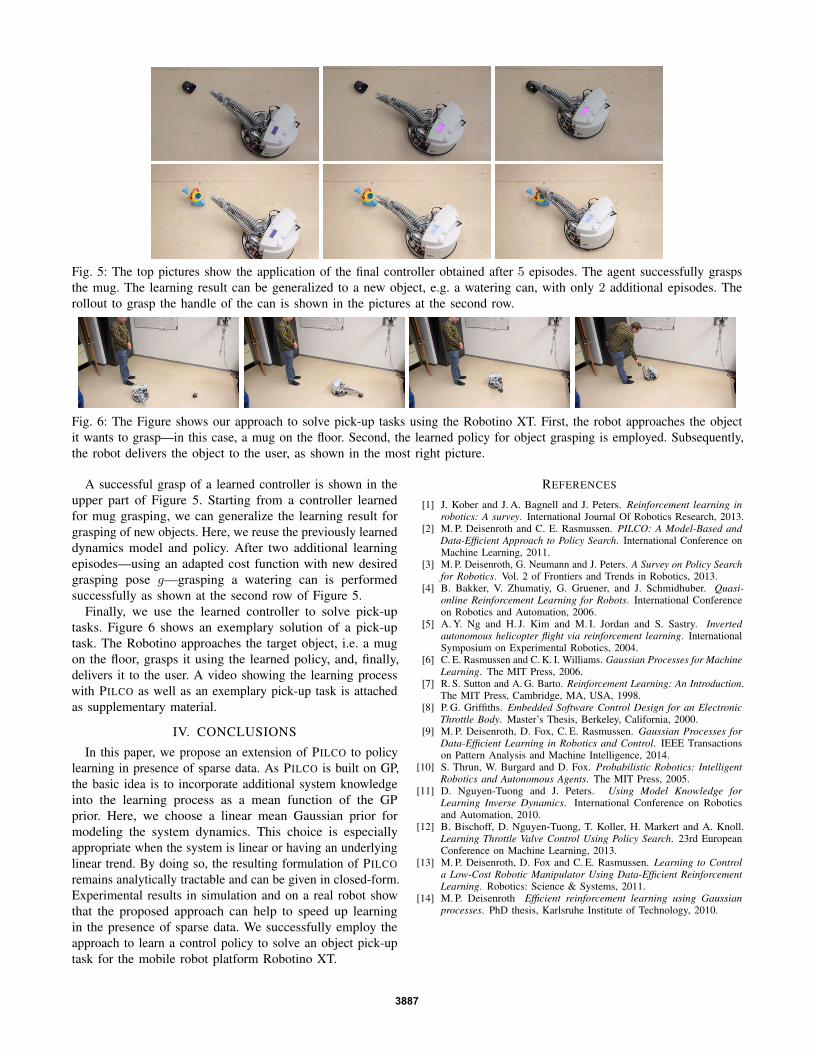
Fig. 5: The top pictures show the application of the final controller obtained after 5 episodes. The agent successfully graspsthe mug. The learning result can be generalized to a new object, e.g. a watering can, with only 2 additional episodes. Therollout to grasp the handle of the can is shown in the pictures at the second row.

Fig. 6: The Figure shows our approach to solve pick-up tasks using the Robotino XT. First, the robot approaches the objectit wants to grasp—in this case, a mug on the floor. Second, the learned policy for object grasping is employed. Subsequently,the robot delivers the object to the user, as shown in the most right picture.

A successful grasp of a learned controller is shown in theupper part of Figure 5. Starting from a controller learnedfor mug grasping, we can generalize the learning result forgrasping of new objects. Here, we reuse the previously learneddynamics model and policy. After two additional learningepisodes—using an adapted cost function with new desiredgrasping pose g—grasping a watering can is performedsuccessfully as shown at the second row of Figure 5.

Finally, we use the learned controller to solve pick-uptasks. Figure 6 shows an exemplary solution of a pick-uptask. The Robotino approaches the target object, i.e. a mugon the floor, grasps it using the learned policy, and, finally,delivers it to the user. A video showing the learning processwith PILCO as well as an exemplary pick-up task is attachedas supplementary material.

IV. CONCLUSIONS

In this paper, we propose an extension of PILCO to policylearning in presence of sparse data. As PILCO is built on GP,the basic idea is to incorporate additional system knowledgeinto the learning process as a mean function of the GPprior. Here, we choose a linear mean Gaussian prior formodeling the system dynamics. This choice is especiallyappropriate when the system is linear or having an underlyinglinear trend. By doing so, the resulting formulation of PILCOremains analytically tractable and can be given in closed-form.Experimental results in simulation and on a real robot showthat the proposed approach can help to speed up learningin the presence of sparse data. We successfully employ theapproach to learn a control policy to solve an object pick-uptask for the mobile robot platform Robotino XT.

REFERENCES

[1] J. Kober and J. A. Bagnell and J. Peters. Reinforcement learning inrobotics: A survey. International Journal Of Robotics Research, 2013.

[2] M. P. Deisenroth and C. E. Rasmussen. PILCO: A Model-Based andData-Efficient Approach to Policy Search. International Conference onMachine Learning, 2011.

[3] M. P. Deisenroth, G. Neumann and J. Peters. A Survey on Policy Searchfor Robotics. Vol. 2 of Frontiers and Trends in Robotics, 2013.

[4] B. Bakker, V. Zhumatiy, G. Gruener, and J. Schmidhuber. Quasi-online Reinforcement Learning for Robots. International Conferenceon Robotics and Automation, 2006.

[5] A. Y. Ng and H. J. Kim and M. I. Jordan and S. Sastry. Invertedautonomous helicopter flight via reinforcement learning. InternationalSymposium on Experimental Robotics, 2004.

[6] C. E. Rasmussen and C. K. I. Williams. Gaussian Processes for MachineLearning. The MIT Press, 2006.

[7] R. S. Sutton and A. G. Barto. Reinforcement Learning: An Introduction.The MIT Press, Cambridge, MA, USA, 1998.

[8] P. G. Griffiths. Embedded Software Control Design for an ElectronicThrottle Body. Master’s Thesis, Berkeley, California, 2000.

[9] M. P. Deisenroth, D. Fox, C. E. Rasmussen. Gaussian Processes forData-Efficient Learning in Robotics and Control. IEEE Transactionson Pattern Analysis and Machine Intelligence, 2014.

[10] S. Thrun, W. Burgard and D. Fox. Probabilistic Robotics: IntelligentRobotics and Autonomous Agents. The MIT Press, 2005.

[11] D. Nguyen-Tuong and J. Peters. Using Model Knowledge forLearning Inverse Dynamics. International Conference on Roboticsand Automation, 2010.

[12] B. Bischoff, D. Nguyen-Tuong, T. Koller, H. Markert and A. Knoll.Learning Throttle Valve Control Using Policy Search. 23rd EuropeanConference on Machine Learning, 2013.

[13] M. P. Deisenroth, D. Fox and C. E. Rasmussen. Learning to Controla Low-Cost Robotic Manipulator Using Data-Efficient ReinforcementLearning. Robotics: Science & Systems, 2011.

[14] M. P. Deisenroth Efficient reinforcement learning using Gaussianprocesses. PhD thesis, Karlsruhe Institute of Technology, 2010.

3887