Polhode Motion, Trapped Flux, and the GP-B Science Data

HEPL SeminarJuly 8, 2009 • Stanford University

Polhode Motion, Trapped Flux, and the GP-B Science Data Analysis

Alex Silbergleit, John Conklinand the Polhode/Trapped Flux Mapping Task Team

HEPL Seminar

2

July 8, 2009 • Stanford University

Outline1. Gyro Polhode Motion, Trapped Flux, and GP-B Readout

(4 charts)2. Changing Polhode Period and Path: Energy Dissipation

(4 charts)3. Trapped Flux Mapping (TFM): Concept, Products,

Importance (7 charts)4. TFM: How It Is Done - 3 Levels of Analysis (11 charts)

A. Polhode phase & angleB. Spin phaseC. Magnetic potential

5. TFM: Results ( 9 charts)6. Conclusion. Future Work (1 chart)

HEPL Seminar

3


Outline1. Gyro Polhode Motion, Trapped Flux, and GP-B Readout 2. Changing Polhode Period and Path: Energy Dissipation 3. Trapped Flux Mapping (TFM): Concept, Products,

Importance4. TFM: How It Is Done - 3 Levels of Analysis


5. TFM: Results 6. Conclusion. Future Work

HEPL Seminar

4


1.1 Free Gyro Motion: Polhoding

• Euler motion equations – In body-fixed frame:– With moments of inertia:

– Asymmetry parameter:

(Q=0 – symmetric rotor)

• Euler solution: instant rotation axisprecesses about rotor principal axisalong the polhode path (angular velocity Ωp)

• For GP-B gyros

HEPL Seminar

5


1.2 Symmetric vs. Asymmetric Gyro Precession

• Symmetric ( Q=0):

γp= const (ω3=const, polhode path=circular cone),

motion is uniform,

φp(t) is linear function of time

• Asymmetric ( Q>0):

Why is polhoding important for GP-B data analysis? Main reason: SQUID Scale Factor Variations due to Trapped Flux

,constpp =Ω=•

φ

,21 II ≠

uniformnonismotion

linearnonistconstcircularnot

ispathpolhodeconstconst

pp

p

−

≠

≠≠•

,)(,),

,( 3

φφ

ωγ

,21 II =

HEPL Seminar

6


1.3 GP-B Readout: London Moment & Trapped Flux

• SQUID signal ~ magnetic flux through pick-up loop (rolls with the S/C):– from dipole field of London Moment (LM) aligned with spin– from multi-pole Trapped Field (point sources on gyro surface – fluxons)

• LM flux - angle between LM and pick-up loop ( β~10-4 , carries relativity signal at low roll frequency ~ 0.01 Hz)

• Fluxons – frozen in rotor surface spin, with it; transfer function ‘fluxon position – pick-up

loop flux’ strongly nonlinear– Trapped Flux (TF) signal contains multiple harmonics of spin; spin axis moves

in the body (polhoding)– amplitudes of spin harmonics are modulated by polhode frequency

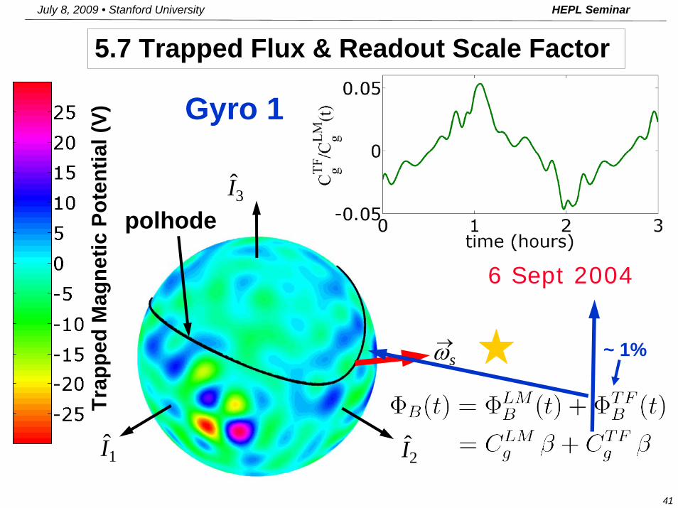
• LM flux and LF part of Trapped Flux (n=0) combine to provideLOW FREQUENCY SCIENCE READOUT (TF LM Flux):

)()( tCt LMg

LM β=Φ

)()(;)()()()()()( 0 thtCttCtCttt TFg

TFg

LMg

TFDC

LMLF ≡+=Φ+Φ=Φ ββ

05.0≤

∑∑∑=

±−

=

±−±− +==Φevenn

inn

oddn

inn

n

inn

TF rsrsrs ethtetHetHt )()()( )()()()()( φφφφφφ β

HEPL Seminar

7


1.4 GP-B High Frequency Data

• HF SQUID Signals– FFT of first 6 spin harmonics– ‘snapshot’: ~ 2 sec of SQUID signal

sampled at 2200 Hz

• Both available during GSI only;~1 snapshot in 40 sec; up to 2 daygaps in snapshot series

• FFT analyzed during the mission• 976,478 snapshots processed

after the mission [harmonics Hn(t)]

• LF SQUID signal (taken after additional 4 Hz LP filter)is used for relativistic drift determination (‘science signal’)

Gyro 1 snapshot, 10 Nov. 2004

HEPL Seminar

8


Outline1. Gyro Polhode Motion, Trapped Flux, and GP-B

Readout2. Changing Polhode Period and Path: Energy

Dissipation3. Trapped Flux Mapping (TFM): Concept, Products,




HEPL Seminar

9


2.1 Discovery: Changing Polhode Period- from Two Sources (HF FFT- red, SRE snapshots - blue)

Also confirmed by the analysis of gyro position signal

HEPL Seminar

10


2.2 Explanation of Changing Polhode Period: Kinetic Energy Dissipation

• Classical polhode paths (blue) for given angular momentum and various energies: intersection of ellipsoids L2 = const and E = const (no dissipation)

• Dissipation: L conserved, but E goes down slowly, then…

• The system slips from a curve to the nearby one with a lower energy (each path corresponds to some energy value). So the long-term path projected on {x–y} plane becomes a tight in-spiral, instead of an ellipse.

A(I2 - I1)/(I3 –I1) = Q2 = 0.5

233

222

211

23

23

22

22

21

21

2

2 ωωω

ωωω

IIIE

IIIL

++=

++=

HEPL Seminar

11


2.3 Explanation (contd.): Kinetic Energy Dissipation

• Dissipation moves spin axis in the body to the maximum inertia axis I3where energy is minimum, under conserved angular momentum constraint

• Relative total energy loss from min, I1, to max, I3, inertia axis is:

for GP-B gyros!

• The total energy loss in GP-B gyros needed to move spin axis all the way from min to max inertia axis is thus less than 4 μJ (E ~ 1 J); in one year, the average dissipation power need for this is just 10-13 W !

• General dissipation model is found in the form of an additional term in the Euler motion equations (unique up to a scalar factor).

• Fitting the model polhode period time history to the measured one allowed the determination the rotor asymmetry parameter Q2 (also from gyro position signal), the asymptotic polhode period Tpa ~ 1-2 hr, and the characteristic time of dissipation τdis~ 1-2 months (for each gyro)

63131313311 104/)(/)( −×≤−=−⇒== IIIEEEIIL ωω

HEPL Seminar

12


2.4 Dissipation Modeling: Products

Dissipation is slow (Tp<<τdis),so the polhode motion of GP-B gyros is quasi-adiabatic

Gyro 1 Gyro 2 Gyro 3 Gyro 4

Tpa (hrs) 0.867 2.581 1.529 4.137

Tp (hrs)

(9/4/2004)2.14 9.64 1.96 5. 90

τdis (days) 31.9 74.6 30.7 61.2

1. Asymptotic Polhode Period and Dissipation Time

2. Polhode phase and angle for the whole mission for each gyro (not perfectly accurate, but enough to start science analysis and TFM)

HEPL Seminar

13








HEPL Seminar

14


3.1 Trapped Flux Mapping (TFM): Concept• Trapped Flux Mapping: finding distribution of trapped

magnetic field and characteristics of gyro motion from odd spin harmonics of HF SQUID signal by fitting to their theoretical model

• Scalar magnetic potential in the body-fixed frame is

• If fluxon number and positions were known, then coefficients Alm are found uniquely by this formula; in reality, coefficients Alm to be estimated by TFM

HEPL Seminar

15


3.2.TFM Concept: Key Points• HF SQUID signal and its preparation for TFM

• TFM is linear fit of Alm coefficients to odd spin harmonics using their theoretical expressions

• Knowing Alm, φp & γp, can predict scale factor due to TF

, n odd

measured →

measured data nonlinear parameters linear parameters

HEPL Seminar

16


3.3 TFM: Products

• For each gyro/entire mission, TFM provides:– Rotor spin speed to ~ 10 nHz– Rotor spin down rate to ~ 1 pHz/s– Rotor spin phase to ~ 0.05 rad– Rotor asymmetry parameter Q2

– Polhode phase to ~ 0.02 rad (10)– Polhode angle to ~ 0.01 – 0.1 rad– Polhode variations of SQUID scale factor [i.e., Trapped Flux

scale factor, ])(tCTFg

HEPL Seminar

17


.Gyro 1 scale factor variations, 8 Oct. 2004, rev 13

3.4 Scale Factor Variations (Nov. 2007)

Fit residuals = 14%

HEPL Seminar

18


Gyro 1 scale factor variations, 8 Oct. 2004, rev 38.

3.5 Scale Factor Variations (Aug. 2008)

Fit residuals = 1%

HEPL Seminar

19


• LF science signal analysis cannot be done w/o accurate polhode phase and angle from TFM (determination of scale factor polhode variations)

• Patch effect torque modeling also cannot be done w/o accurate polhode phase and angle from TFM (all the torque coefficients are modulated by polhode frequency harmonics, same as the scale factor is)

• TFM produces those polhode variations of scale factor from HF SQUID data (independent of LF science analysis)

– Allows for separate determination of the London Moment scale factor and D.C. part of Trapped Flux scale factor slowly varying due to energy dissipation

(next slide)

– When used in LF science analysis, simplifies it significantly (dramatically reduces the number of estimated parameter, makes the fit linear)

3.6 TFM: Importance – Scale Factor & Torque

HEPL Seminar

20


• SQUID Scale Factor, Cg(t) = CgLM + Cg

TF(t)Cg

TF(t) contains polhode harmonics & D.C. part

3.7 TFM Importance: D.C. Part of Scale Factor

D.C. Part of Gyro 2 Scale Factor

2Ωp = Ωorbit

S/C anomaly

With CgTF(t) known through the mission,

CgLM can be determined to ~ 3×10-5

HEPL Seminar

21


GP-B Polhode/TFM Task Team

with advising and participation of:

David SantiagoAlex SilbergleitPaul WordenDan DeBra Mac Keiser

Michael Dolphin Jonathan KozaczukMichael Salomon John Conklin

Francis Everitt Michael Heifetz Vladimir SolomonikTom Holmes John Turneaure

HEPL Seminar

22





Importance4. TFM: How It Is Done. 3 Levels of Analysis



HEPL Seminar

23


4.1 TFM & Scale Factor Cg Modeling OverviewMeasured HF SQUID signal

Spin speed, ωs , phasePolhode period TpComplex Spin Harmonics Hn

CgTF(t)

LF ScienceAnalysis

Measured LF SQUID signal

Cgcomparison

GSS data

CLFg(t)

Trapped Flux

Mapping

Q2

green

Input to LF analysis

Main TFM output

Data

Non HF analysis

LegendPolhode phase φp, polhode angle γp

HEPL Seminar

24


4.2 TFM Methodology• Expand scalar magnetic potential in spherical harmonics• Fit theoretical model to odd harmonics of spin,

accounting for polhode & spin phase• 3 Level approach

– Level A – Independent day-to-day fits,determine best polhode phase φp & angle γp (nonlinear)

– Level B – Consistent best fit polhode phase & angle,independent day-to-day fits for spin phase φs (nonlinear)

– Level C – With best fit polhode phase, angle & spin phase,fit single set of Alms to long stretches of data (linear)

» Compare spin harmonics to fit over year, refine polhode phase

Iterative refinement of polhode phase & Alms

HEPL Seminar

25


• Level A input:– Measured spin harmonics Hn from HF SQUID signal (n odd)– Measured polhode frequency– Measured spin speed

• Fit 1-day batch ⇒ initial polhode phase for each batch • Build ‘piecewise’ polhode phase for the entire mission,

accounting for 2π ambiguities• Fit exponential model to polhode phase & compute angle

• Level A output:– consistent polhode phase & angle for entire mission

4.3 Level A: Polhode Phase φp & Angle γp

from dissipation model

zero when Q2=0

HEPL Seminar

26


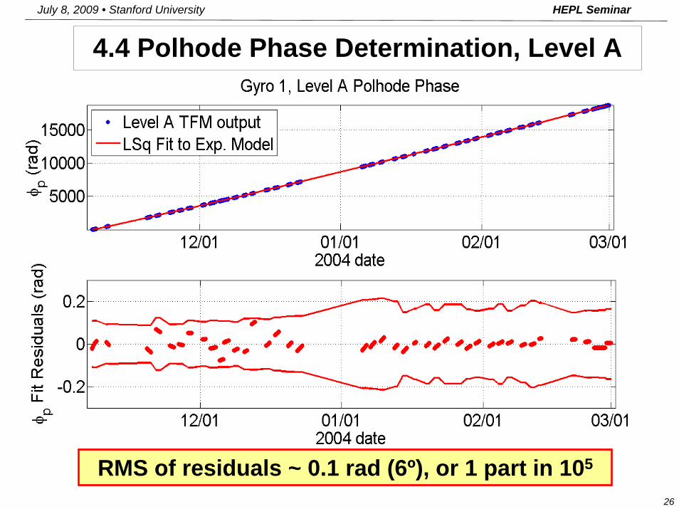
4.4 Polhode Phase Determination, Level A

RMS of residuals ~ 0.1 rad (6º), or 1 part in 105

HEPL Seminar

27


4.5 Level B: Spin Phase φs Estimation

• Level B input:– Best-fit, consistent polhode phase & angle from Level A– Measured spin harmonics Hn (n odd) from HF SQUID signal– Measured spin speed

• Fit quadratic model for spin phase, once per batch

• Level B output:– Rotor spin speed to ~ 10 nHz– Rotor spin-down rate to ~ 1 pHz/s– Rotor spin phase to ~ 0.05 rad (3°)

polhode phasew/o asymmetry correction

HEPL Seminar

28


4.6 Gyro 1 Fit to H5 with & without Extra Term

WITHOUT Δφs(t, Q)

WITH Δφs(t, Q)

Post-fit residuals reduced by factor of 2-4

HEPL Seminar

29


4.7 Gyro 1 Fit to H5 with & without Extra Term

WITHOUT Δφs(t, Q)

WITH Δφs(t, Q)

Post-fit residuals reduced by factor of 2-4

HEPL Seminar

30


4.8 Level C: Alm & Polhode Phase Refinement• Level C input:

– Best-fit, consistent polhode phase & angle, Q2 - from Level A– Spin phase from Level B– Measured spin harmonics Hn from HF SQUID signal (n odd)

• Linear LSQ fit over entire mission ⇒ Alm’s• Level C output:

– Coefficients of magnetic potential expansion, Alm

– Refined polhode phase & angle

• Polhode phase refinement– Complex Hn, accounting for elapsed spin phase, required for linear fit– Amplitude of spin harmonics |H1| unaffected by spin phase errors

⇒ |H1| most reliable, only contains Alm’s & polhode phase φp

– Assume Alm’s correct, adjust polhode phase to match data & iterate

HEPL Seminar

31


4.9 Polhode Phase Refinement (Level C)

In phase

Gyro 1, October 2004

Phase slip

Gyro 1, September 2004

1. Compare amplitude of spin harmonic |H1| to reconstructed version from best-fit parameters

2. Adjust polhode phase to match

Provides most accurate estimate of polhode phase

HEPL Seminar

32


4.10 Iterative Polhode Phase Refinement• With new polhode phase, re-compute spin phase, Alm’s,

Successive iterations show convergence

iteration 0iteration 1iteration 2

Gyro 3 polhode phase refinement

HEPL Seminar

33


4.11 Polhode Phase Error Model (Level C)

• Polhode phase correction (from |H1|) fit to exp. model

• Post-fit residuals fit to Fourier expansion

gyro 1 polhode phase refinement residuals

50 mrad RMS

5 mrad RMS

1 part in 105 fit becomes 1 part in 106

gyro 1 polhode phase error model residual

HEPL Seminar

34





Importance4. TFM: How It Is Done. 3 Levels of Analysis


5. TFM: Results6. Conclusion. Future Work

HEPL Seminar

35


5.1 Rotor Asymmetry Parameter Q2 (from Level A)

Method Gyro 1 Gyro 2 Gyro 3 Gyro 4

TFM 0.303 ± 0.069 0.143 ± 0.029 0.127 ± 0.072 0.190 ± 0.048

Previous work

0.33(0.29 – 0.38)

0.36(0.14 – 0.43) ~ 0 0.32

(0.30 – 0.40)

• CgTF and Hn are relatively insensitive to Q2

– Q2 estimation accurate to ~ 20%– Adequate for TFM

HEPL Seminar

36


5.2 Q2 Results & Probability Distribution Function

• Observation: 0.12 < Q2 < 0.31 all gyros

HEPL Seminar

37


5.3 Spin-Down Rate to ~ 1 pHz/s (from Level B)

Consistent withpatch effect

HEPL Seminar

38


5.4 Spin Speed and Spin-Down Time (from Level B)

Parameter Gyro 1 Gyro 2 Gyro 3 Gyro 4

fs (Hz) 79.40 61.81 82.11 64.84

τ sd (yrs) 15,800 13,400 7,000 25,700

HEPL Seminar

39


5.5 Alms for Gyro 1 (from Level C)

HEPL Seminar

40


5.6 Distribution of Alm Values

• Fits indicate Alms follow zero mean Gaussian distribution, that also agrees with physical understanding of trapped flux

• Assuming Alms normally distributed about zero allowed for more accurate estimates of coefficients with higher indices

Ν (µ = 0 V, σ = 0.87 V)

HEPL Seminar

41


6 Sept 2004

Trap

ped

Mag

netic

Pot

entia

l (V)

I2

I3

I1

ωs→

Gyro 1

polhodeˆ

ˆ ˆ

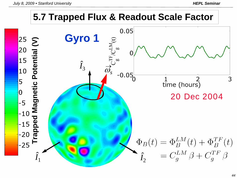
5.7 Trapped Flux & Readout Scale Factor

~ 1%

HEPL Seminar

42


4 Oct 2004

Trap

ped

Mag

netic

Pot

entia

l (V)

I2

I3

I1

Gyro 1

ˆ

ˆ ˆ

ωs→


HEPL Seminar

43


Trap

ped

Mag

netic

Pot

entia

l (V)

I2

I3

I1

Gyro 1

ˆ

ˆ ˆ

ωs→

14 Nov 2004


HEPL Seminar

44


Trap

ped

Mag

netic

Pot

entia

l (V)

I2

I3

I1

Gyro 1

ˆ

ˆ ˆ

ωs→

20 Dec 2004


HEPL Seminar

45


20 Feb 2005

Trap

ped

Mag

netic

Pot

entia

l (V)

I2

I3

I1

Gyro 1

ˆ

ˆ ˆ

ωs→


HEPL Seminar

46


26 June 2005

Trap

ped

Mag

netic

Pot

entia

l (V)

I2

I3

I1

Gyro 1

ˆ

ˆ ˆ

ωs→


HEPL Seminar

47


5.8 Scale Factor Results, Nov. ‘07 vs. Aug. ‘08

Gyro Data Used

Relative residuals

(rms)Number of Harmonics

Relative Amplitude of

Variations

CgTF Error

Relative to Cg(formal sigmas)

Oct. 14% 11 0.6×10-2 - 2×10-2

1 3% to 0.2%full year 1.1% 21 1.5×10-4 - 7.0×10-5

Sept. -Dec. 15% 17 3×10-4 - 6×10-4

2 1.5% to 0.5%full year 1.5% 25 6.0×10-5 - 3.0×10-5

Sept. -Dec. 6% 5 3×10-3 - 4×10-3

3 1% to 0.01%full year 2.6% 21 2.0×10-4 - 1.6×10-4

Oct. -Dec. 17% 9 3×10-3 - 7×10-3

4 0.3% to 0.1%full year 2.8% 21 8.5×10-5 - 6.5×10-5

HEPL Seminar

48


5.9 TFM & LF Cg Comparison Cg variationsLF–TFM 11/07LF–TFM 9/08

HEPL Seminar

49


6. Conclusion. Future Work• Polhode period and path change observed on orbit are

explained by rotation energy loss and properly analyzed, laying ground for Trapped Flux Mapping

• The results of Trapped Flux Mapping based on oddharmonics of HF SQUID signal are crucial for getting the best measurement of relativistic drift rate (determining LF scale factor variations and patch effect torque in science analysis)

• Future work on examining even HF harmonics might lead to new important results, such as:– Estimation of SQUID signal nonlinearity coefficients– Alternative science signal, i. e., independent determination of

spin–to–pick-up loop misalignment time history

HEPL Seminar

50


GP-B Polhode/TFM Task Team

with advising and participation of:

David SantiagoAlex SilbergleitPaul WordenDan DeBra Mac Keiser

Michael Dolphin Jonathan KozaczukMichael Salomon John Conklin

Francis Everitt Michael Heifetz Vladimir SolomonikTom Holmes John Turneaure

HEPL Seminar

51


Backup slides …

HEPL Seminar

52


IL

LL

LE

IIIIIIIIkKT

ELI

IIII

QQ

IIIIIIIIk

ll

p =⋅

==−−

=

=−−

−=

−−−−

=

rrωω

ω2,

))(()(4

2,

)()(

1))(())((

123

321

2

1

32

2

123

3122

Elliptic Functions and Parameters in Free Gyro Motion

HEPL Seminar

53


Dissipation Model

• For GP-B gyros variation of both frequency and energy is very small, so

with parameter μ0 to be estimated from the measured data (e.g., polhode period time history)

• Dot product with and gives, respectively, the angular momentum conservation and the energy evolution equation:

• Euler equation modified for dissipation (unique up to a factor μ):

Lr

ωr

HEPL Seminar

54


Scale Factor Formal Errors

~ 100x

~ 20x

~ 5x

~ 50x

LF Analysis TFM 11/07TFM 09/08

Documents

Polhode Motion, Trapped Flux, and the GP-B Science Data