Polarization amidst poverty reduction: A case study

of Nigeria and Ghana∗

Fabio Clementi†

University of Macerata, Macerata, Italy

Vasco Molini

World Bank, Washington DC, USA

Francesco Schettino

Second University of Naples, Naples, Italy

July 30, 2016

∗The authors acknowledge financial support from the World Bank. We thank Federica Alfani (Foodand Agriculture Organization of the United Nations), Dan Pavelesku, Rose Mungai and Ayago E. Wambile(World Bank) for excellent assistance with data preparation. We also thank Christoph Lakner, PierellaPaci and Andrew Dabalen (World Bank) for comments on an earlier version of the manuscript. Of course,we are the sole responsible for all possible errors the paper may contain.†Corresponding author : fabio.clementi@unimc.it.

Abstract

Despite sustained real growth over recent decades, reduction in official poverty rates in Nigeria

and Ghana has not been up to general expectations. The lack of a faster reduction in poverty

despite a significant growth in GDP may be due to an increase in inequality. The latter is,

however, just one aspect of the problem. A complementary hypothesis is that both Nigeria and

Ghana are also experiencing increasing polarization.

This paper uses newly available data and the relative distribution methodology (Handcock

and Morris, 1998, 1999) to present new results on polarization in Nigeria and Ghana. The

findings confirm the hypothesis that both the countries are going through a process of economic

polarization. Compared to 2003, the distribution of consumption in Nigeria has become more

concentrated in upper and lower deciles in 2013, while the middle deciles have thinned. A

between-group analysis shows the emergence of a macro-regional gap: while the South-South

and South-West regions contribute mainly to polarization in the upper tail, households in the

North East and North West zones—the conflict-stricken areas—are more likely to fall in the lower

national deciles. Likewise, the distributional changes occurred over the last 20 years hollowed out

the middle of the Ghanaian household consumption distribution and increased the concentration

of households around the highest and lowest deciles. When looking at the drivers of polarization,

household characteristics, educational attainment and access to basic infrastructures all tended

to increase over time the size of the upper and lower tails of the consumption distribution, and

as a consequence the degree of polarization.

JEL classification: C14; D31; D63

Keywords: Nigeria; Ghana; consumption expenditure; poverty and inequality; polarization; relative dis-

tribution; decomposition analysis

1

2 F. Clementi, V. Molini, and F. Schettino

1 Introduction

Nigeria and Ghana have been before 2015 among the fastest growing economies in Sub-Saharan

Africa (SSA), with per capita growth rates averaging 5–6%. In the last decade they also managed

to reduce poverty substantially. In Nigeria, the poverty rate in per capita terms declined by 10

percentage points, from 46% in 2004 to 36.1% in 2013. In Ghana, poverty declined from 28% in

2005 to 21% in 2013.

In both countries, however, in the last decade poverty reduction was not commensurate with

the fast GDP growth. Compared with the rest of SSA and other low-middle-income (LMI)

countries, poverty reduction in Nigeria and Ghana has been less responsive to economic growth.

Growth to poverty elasticity (GEP) estimates indicate that for every 1% growth in GDP per

capita, poverty declined by only 0.6% in Nigeria and 0.7% in Ghana. Both countries’ growth

elasticity to poverty is half of that of the SSA average and only one fourth of that of LMI

countries. The GEP was also lower than that of a number of African countries, such as Rwanda

and Ethiopia, which enjoyed high growth rates in the last decade.

Three factors determined this low responsiveness in the last decade. First, high growth

rates have been accompanied by comparatively high rates of population growth. Population, in

particular in Nigeria, has been growing at an average rate of 2.7% per year and fertility rates

remain particularly high. Second, like other resource-rich economies in the developing world,

Nigeria and Ghana shows a low labour absorptive capacity. Third, inequality has been growing

and has adversely affected poverty reduction; in Nigeria only half of the consumption per capita

growth translated into poverty reduction, and in Ghana only 70%.

Despite the different sizes, the similarities between the two countries do not end here. Both,

during the period of fast growth and poverty reduction, experienced a rapid increase in wel-

fare polarization driven—in particular in Nigeria—by the increasing divide between Northern

and Southern parts of the countries (Aigbokhan, 2000; Araar, 2008; Awoyemi and Araar, 2009;

Awoyemi et al., 2010; Ogunyemi and Oni, 2011; Ogunyemi et al., 2011; Ogunyemi, 2013; Clementi

et al., 2014, 2015; Molini and Paci, 2015; Clementi et al., 2016; World Bank, 2016). Polariza-

tion is the combination of the divergence from the global mean income and the convergence

toward local mean incomes; it differs from inequality because the latter is the overall dispersion

of the distribution, that is, the distance of every individual from the median or mean income. In

income-polarized societies, people are clustered around the group means and tend to be remote

from the mean or median of the overall distribution. Within each group, there is income homo-

geneity and often narrowing income inequality. Thus, we may talk of increasing “identification”.

Between the two groups, we talk, rather, about increasing “alienation” (Duclos et al., 2004). The

overall impact of the forces of identification and of alienation between two groups of significant

size leads to effective opposition, a situation that may give rise to social tensions and conflict

(Esteban and Ray, 1999, 2008, 2011). Also, the group at the top of the distribution possesses

voice, while the other group, which is made up of those at the bottom, are voiceless in matters

that affect their welfare and society at large.

The present study adds to the existing literature on inequality, polarization and poverty

in Nigeria and Ghana on a number of fronts. First, it uses a very intuitive yet little explored

method, the “relative distribution” introduced by (Handcock and Morris, 1998, 1999), to analyze

Polarization amidst poverty reduction: A case study of Nigeria and Ghana 3

the recent distributional changes occurred in the Nigeria and Ghana. The strength of this method

consists in providing a non-parametric framework for taking into account all the distributional

differences that could arise in the comparison of distributions over time and space. In this way, it

enables to summarize multiple features of the expenditure distribution that would not be detected

easily from a comparison of standard measures of inequality and polarization. Second, another

goal of this paper is to document not just national, but also sub-national patterns of polarization.

Nigeria and Ghana are highly heterogeneous, so that drivers of polarization can indeed differ

across macro regions. Finally, the paper develops within the relative distribution framework a

novel methodology to identify the drivers of distributional changes and quantify their impact on

the welfare distribution—the main value added being it enables a very granular analysis of the

distributional changes that an analysis based on standard inequality decompositions would not

allow.

The paper is organized as follows. Section 2 reviews the approaches to measuring economic

polarization. Section 3 outlines the distinctive features of the relative distribution methodology

and presents the new decomposition method used to identify the drivers of polarization. Section

4 discusses the data. Section 5 details the main findings of the study. Section 6 concludes.

2 Some background on the income polarization literature

Over the last two decades, the issue of polarization has come to be assigned increasing importance

in the analysis of income distribution. Notwithstanding the pains the polarization literature has

suffered to distinguish itself from pure inequality measurement—see e.g. Foster and Wolfson

(1992), Levy and Murnane (1992), Esteban and Ray (1994) and Wolfson (1994, 1997)—it now

seems to be fairly widely accepted that polarization is a distinct concept from inequality.

Broadly speaking, the notion of polarization is concerned with the disappearance of the mid-

dle class, which occurs when there is a tendency to concentrate in the tails—rather than the

middle—of the income distribution. One of the main reasons for looking at income polarization

this way, which is usually referred to as “bi-polarization”, is that a well-off middle class is impor-

tant to every society because it contributes significantly to economic growth, as well as to social

and political stability (e.g. Easterly, 2001, Pressman, 2007, and Birdsall, 2010). In contrast, a

society with high degree of income polarization may give rise to social conflicts and tensions.

Therefore, in order for such risks to be minimized, it is necessary to monitor the economic evo-

lution of the society using indices that look at the dispersion of the income distribution from the

middle toward either or both of the two tails. Measures of income polarization that correspond

to this case have been proposed in the literature by Foster and Wolfson (1992), Wolfson (1994,

1997), Wang and Tsui (2000), Chakravarty and Majumder (2001), Rodrıguez and Salas (2003),

Chakravarty et al. (2007), Silber et al. (2007), Chakravarty (2009), Chakravarty and D’Ambrosio

(2010), Lasso de la Vega et al. (2010), and others.

A more general notion of income polarization, which was originally proposed by Esteban

and Ray (1994), regards the latter as “clustering” of a population around two or more poles of

the distribution, irrespective of where they are located along the income scale. The notion of

income polarization in a multi-group context is an attempt at capturing the degree of potential

conflict inherent in a given distribution (see Esteban and Ray, 1999, 2008, 2011). The idea is to

4 F. Clementi, V. Molini, and F. Schettino

consider society as an amalgamation of groups, where the individuals in a group share similar

attributes with the other members (i.e. have a mutual sense of “identification”) but in terms of

the same attributes they are different from the members of the other groups (i.e. have a feeling

of “alienation”). Political or social conflict is therefore more likely the more homogeneous and

separate the groups are, that is when the within-group income distribution is more clustered

around its local mean and the between-group income distance is longer. In addition to Esteban

and Ray (1994), indices regarding the concept of income polarization as conflict among groups

have been investigated, among others, by Gradın (2000), Milanovic (2000), D’Ambrosio (2001),

Zhang and Kanbur (2001), Reynal-Querol (2002), Duclos et al. (2004), Lasso de la Vega and

Urrutia (2006), Esteban et al. (2007), Gigliarano and Mosler (2009) and Poggi and Silber (2010).

Much of the literature so far considered has analyzed summary measures of income polar-

ization. Another strand uses kernel density estimation and mixture models in order to describe

changes in polarization patterns over time, not just of personal incomes (as in Jenkins, 1995,

1996, Pittau and Zelli, 2001, 2004, 2006, and Conti et al., 2006) but also of the cross-country

distribution of per capita income (see Quah, 1996a,b, 1997, Bianchi, 1997, Jones, 1997, Paap

and van Dijk, 1998, Johnson, 2000, Holzmann et al., 2007, Henderson et al., 2008, Pittau et al.,

2010, Anderson et al., 2012, and others). The analysis of the shape of the income distribution

provides indeed a picture from which at least three important distributional features can be

observed simultaneously (Cowell et al., 1996): income levels and changes in the location of the

distribution as a whole; income inequality and changes in the spread of the distribution; clump-

ing and polarization as well as changes in patterns of clustering at different modes. Finally, a

rather recent (yet non-parametric) approach that combines the strengths of summary polariza-

tion indices with the details of distributional change offered by the kernel density estimates—the

so-called “relative distribution”—has been employed by Alderson et al. (2005), Massari (2009),

Massari et al. (2009a,b), Alderson and Doran (2011, 2013), Borraz et al. (2013), Clementi and

Schettino (2013, 2015), Clementi et al. (2014, 2015, 2016), Molini and Paci (2015), Petrarca and

Ricciuti (2015) and Nissanov and Pittau (2016) to assess the evolution of the middle class and

the degree of household income polarization in a number of middle- and high-income countries

in the world.

3 Relative distribution methods

3.1 The relative distribution: basic concepts

In the current application, the relative distribution approach has some important advantages

over the other mentioned methods of investigating income polarization. First, it readily lends

itself to simple and informative graphical displays of relative data that reveal precisely where and

by how much an income distribution changed over time. Second, by providing the potential for

decomposition into location and shape components, it allows one to examine several hypotheses

regarding the origins of distributional change—such as whether the change consists of an equal

absolute subtraction or addition to all incomes that moves the overall distribution either to

the left or to the right (while leaving the shape unaltered) or of shape modifications which,

Polarization amidst poverty reduction: A case study of Nigeria and Ghana 5

by definition, are independent of location shifts.1 Lastly, it allows us to quantify the degree of

polarization due to changes in distributional shape only (i.e. net of location shifts), thus enabling

one to isolate aspects of inter-distributional inequality that are often hidden when also changes

in location are examined.

Basically, the relative distribution method can be applied whenever the distribution of some

quantity across two populations is to be compared, either cross-sectionally or over time.2 To

proceed, it is necessary to single out one of the two populations, refer to it as the “comparison”

population, and refer to the other as the “reference” population. More formally, let Y0 be

the income variable for the reference population and Y the income variable for the comparison

population. The relative distribution of Y to Y0 is defined as the distribution of the random

variable:

R = F0 (Y ) , (1)

which is obtained from Y by transforming it by the cumulative distribution function of Y0, F0.

As a random variable, R is continuous on the outcome space [0, 1], and its realizations, r, are

referred to as “relative data”. Intuitively, the relative data can be interpreted as the set of

positions that the income observations of the comparison population would have if they were

located in the income distribution of the reference population. The probability density function

of R, which is called the “relative density”, can be obtained as the ratio of the density of the

comparison population to the density of the reference population evaluated at the relative data

r:

g (r) =f(F−1

0 (r))

f0

(F−1

0 (r)) =

f (yr)

f0 (yr), 0 ≤ r ≤ 1, yr ≥ 0, (2)

where f (·) and f0 (·) denote the density functions of Y and Y0, respectively, and yr = F−10 (r)

is the quantile function of Y0. The relative density has a simple interpretation, as it describes

where households at various quantiles in the comparison distribution are concentrated in terms

of the quantiles of the reference distribution. As for any density function, it integrates to 1 over

the unit interval, and the area under the curve between two values r1 and r2 is the proportion

of the comparison population whose income values lie between the r1th and r2

th quantiles of the

reference population.

When the relative density function shows values near to 1, it means that the two populations

have a similar density at the rth quantile of the reference population, and thus R has a uniform

distribution in the interval [0, 1]. A relative density greater than 1 means that the comparison

population has more density than the reference population at the rth quantile of the latter.

Finally, a relative density function less than 1 indicates the opposite. In this way one can

distinguish between growth, stability or decline at specific points of the income distribution.

1Of course, both the location and shape effects—named respectively as “growth” and “inequality” (or “distribu-tional”) effect (Kakwani, 1993; Bourguignon, 2003, 2004)—may also concur together in producing the distributionalchange.

2Here we limit ourselves to illustrating the basic concepts behind the use of the relative distribution method.Interested readers are referred to Handcock and Morris (1998, 1999; but see also Hao and Naiman, 2010, ch. 5) fora more detailed explication and a discussion of the relationship to alternative econometric methods for measuringdistributional differences. A method very similar in spirit to the relative distribution has recently been developedby Silber et al. (2014).

6 F. Clementi, V. Molini, and F. Schettino

3.2 The location/shape decomposition of the relative distribution

As we have said before, one of the major advantages of this method is the possibility to decompose

the relative distribution into changes in location, usually associated with changes in the median

(or mean) of the income distribution, and changes in shape (including differences in variance,

asymmetry and/or other distributional characteristics) that could be linked with several factors

like, for instance, polarization. Formally, the decomposition can be written as:

g (r) =f (yr)

f0 (yr)︸ ︷︷ ︸Overall relative

density

=f0L (yr)

f0 (yr)︸ ︷︷ ︸Density ratio for

the location effect

× f (yr)

f0L (yr)︸ ︷︷ ︸Density ratio forthe shape effect

, (3)

where f0L (yr) = f0 (yr + ρ) is a density function adjusted by an additive shift with the same

shape as the reference distribution but with the median of the comparison one.3 The value ρ is

the difference between the medians of the comparison and reference distributions. If the latter

two distributions have the same median, the density ratio for location differences is uniform

in [0, 1]. Conversely, if the two distributions have different median, the “location effect” is

increasing (decreasing) in r if the comparison median is higher (lower) than the reference one.

The second term, which is the “shape effect”, represents the relative density net of the location

effect and is useful to isolate movements (re-distribution) occurring between the reference and

comparison populations. For instance, we could observe a shape effect function with some sort of

(inverse) U-shaped pattern if the comparison distribution is relatively (less) more spread around

the median than the location-adjusted one. Thus, it is possible to determine whether there is

polarization of the income distribution (increases in both tails), “downgrading” (increases in

the lower tail), “upgrading” (increases in the upper tail) or convergence of incomes towards the

median (decreases in both tails).

3.3 Relative polarization indices

The relative distribution approach also includes a median relative polarization index (MRP),

which is based on changes in the shape of the income distribution to account for polarization.

This index is normalized so that it varies between -1 and 1, with 0 representing no change in

the income distribution relative to the reference year. Positive values represent more polariza-

tion—i.e. increases in the tails of the distribution—and negative values represent less polariza-

tion—i.e. convergence towards the center of the distribution. The MRP index for the comparison

population can be estimated as (Morris et al., 1994, p. 217):

MRP =4

n

(n∑i=1

∣∣∣∣ri − 1

2

∣∣∣∣)− 1, (4)

3Median adjustment is preferred here to mean adjustment because of the well-known drawbacks of the meanwhen distributions are skewed. A multiplicative median shift can also be applied. However, the multiplicativeshift has the drawback of affecting the shape of the distribution. Indeed, the equi-proportionate income changesincrease the variance and the rightward shift of the distribution is accompanied by a flattening (or shrinking) ofits shape (see e.g. Jenkins and Van Kerm, 2005).

Polarization amidst poverty reduction: A case study of Nigeria and Ghana 7

where ri is the proportion of the median-adjusted reference incomes that are less than the ith

income from the comparison sample, for i = 1, . . . , n, and n is the sample size of the comparison

population.

The MRP index can be additively decomposed into the contributions to overall polarization

made by the lower and upper halves of the median-adjusted relative distribution, enabling one to

distinguish downgrading from upgrading. In terms of data, the lower relative polarization index

(LRP) and the upper relative polarization index (URP) can be calculated as follows:

LRP =8

n

n/2∑i=1

(1

2− ri

)− 1, (5)

URP =8

n

n∑i=n/2+1

(ri −

1

2

)− 1, (6)

with MRP = 12 (LRP + URP). As the MRP, LRP and URP range from -1 to 1, and equal 0

when there is no change.

3.4 Adjustment for covariates

Similarly to what is observed for location and shape decomposition, it is possible to adjust

the relative distribution for changes in the distribution of covariates measured on the house-

holds, which often vary systematically by population. The covariate adjustment technique can

be used to separate the impacts of changes in population composition from changes in the

covariate-response relationship.4 This decomposition according to covariates draws on the def-

inition of a counter-factual distribution for the response variable in the reference population

that is composition-adjusted to have the same distribution of the covariates as the comparison

population.

Assume for simplicity that the covariate Z is categorical.5 Let{π0k

}Kk=1

and {πk}Kk=1, where

K is the number of categories of the covariate, denote the probability mass functions of Z for

the reference and comparison populations, i.e. their composition according to the covariate. For

conditional comparisons of the response variable Y across the two populations one can consider

the density of Y0 given that Z0 = k:

fY0|Z0(y|k) , k = 1, . . . ,K, (7)

and the density of Y given that Z = k:

fY |Z (y|k) , k = 1, . . . ,K. (8)

4Recently, there have been several papers that have studied decomposition methods to explain changes in theunconditional distribution of an outcome variable due to either changes in the distribution of the covariates, orchanges in the conditional distribution of the outcome given covariates, or both—see for instance the extensivesurvey by Fortin et al. (2011) on the wage decomposition literature. Benefits and drawbacks of some of these meth-ods, and how they are often largely subsumed by the relative distribution framework, are reviewed in Handcockand Morris (1999, ch. 2).

5The extensions to continuous and multivariate covariates are considered in Handcock and Morris (1999, ch.7).

8 F. Clementi, V. Molini, and F. Schettino

These densities represent the covariate-response relationship. The marginal densities of Y0 and

Y can be written, respectively, as:

f0 (y) =K∑k=1

π0kfY0|Z0

(y|k) and f (y) =K∑k=1

πkfY |Z (y|k) . (9)

Then, the counter-factual distribution with the covariate composition of the comparison

population and the covariate-response relationship of the reference population is:

f0C (y) =

K∑k=1

πkfY0|Z0(y|k) , (10)

and can be used to decompose the overall relative distribution into a component that represents

the effect of changes in the marginal distribution of the covariate (the “composition effect”) and

a component that represents the changes in the covariate-response relationship (the “residual

effect”). The decomposition can be represented in the following terms:

g (r) =f (yr)

f0 (yr)︸ ︷︷ ︸Overall relative

density

=f0C (yr)

f0 (yr)︸ ︷︷ ︸Density ratio for

the composition effect

× f (yr)

f0C (yr)︸ ︷︷ ︸Density ratio forthe residual effect

. (11)

Comparison of f (yr) to f0C (yr)—i.e. the residual effect—holds the population composition

constant, and therefore isolate changes of income distribution due to the fact that returns to the

selected covariate changed over time. By contrast, f0C (yr) and f0 (yr) have the same covariate-

response relationship, and the comparison between them—i.e. the composition effect—isolate

the changes due to the different composition of the population under the assumption that the

conditional distribution of income remain unchanged.

3.5 Blinder-Oaxaca type decomposition of location and shape differences

In this section we present a novel method for analyzing the effects of covariates on the observed

distributional changes due to both the location and shape shifts. Novel because in the original

relative distribution framework, the method proposed to measure the impact of polarization

drivers does not provide intuitive results and it is of limited use for policy making purposes. By

contrast, our method that combines the relative distribution approach and the regression based

decompositions, can produce an easily interpretable set of results.

In the relative distribution setting, the exploration of the distributional impacts of changes

in covariates requires that the overall relative density is adjusted for these changes using the

technique described in the previous section. This technique partials out the impact of changes

in the distribution of the covariates—the “composition effect”—and the modifications in the

conditional distributions of household consumption expenditure given the covariate levels—the

“residual effect”. Conceptually, this parallels the traditional regression-based decomposition

that separates changes in covariates (the X’s) from changes in the “returns” to the covariates

(the regression coefficients, or β’s). However, the covariate adjustment technique proposed by

Handcock and Morris does not provide a simple and intuitively accessible way of dividing up the

Polarization amidst poverty reduction: A case study of Nigeria and Ghana 9

changes exclusively due to a location shift or shape differences into the contribution of changes in

the distribution of each single covariate and that of the changing “returns” to the covariates; also,

differently from what happens in the classical regression decomposition approach, its drawback is

making it difficult to summarize the contributions above into a single value as, for example, the

estimated coefficients obtained by the regression procedure would make it possible to quantify.

The framework we propose integrates the spirit of the relative distribution approach and

recent developments from the regression-based decomposition literature. This can be regarded

as an extension of the covariate adjustment technique developed by Handcock and Morris and can

be used to quantify the impact of an arbitrary number of covariates on distributional differences

due to both location and shape shifts, so as to identify the key drivers of these changes.

In detail, we decompose the component relative distributions that represent differences in

location and shape by applying a procedure recently proposed by Firpo et al. (2009) for the

decomposition of wage differentials. The method is based on running unconditional quantile

regressions to estimate the impact of changing the distribution of explanatory variables along

the entire distribution of the dependent variable and using the traditional Blinder (1973) and

Oaxaca (1973) decomposition framework to decompose differentials at selected quantiles of the

consumption distribution.

To estimate the unconditional quantile regression, we have first to derive the re-centered in-

fluence function (RIF) for the τ th quantile of the dependent variable distribution—consumption,

in our case—which can be shown as (Firpo et al., 2009; Essama-Nssah and Lambert, 2012; Fortin

et al., 2011):

RIF (c; qτ , FC) =

qτ + τfC(qτ ) , c > qτ ,

qτ − 1−τfC(qτ ) , c < qτ ,

(12)

where qτ is the sample quantile and fC (qτ ) is the density of consumption C at the τ th quan-

tile. In practice, the RIF is estimated by replacing all unknown quantities by their observable

counterparts. In the case of (12) unknown quantities are qτ and fC (qτ ), which are estimated by

the sample τ th quantile of C and a standard non-parametric kernel density estimator, respec-

tively. Firpo et al. (2009) show that the unconditional quantile regression can be implemented

by running a standard OLS regression of the estimated RIF on the covariates X:6

E [RIF (C; qτ , FC)|X = x] = Xβτ , (13)

where the coefficient βτ represents the approximate marginal effect of the explanatory variable

X on the τ th unconditional quantile of the household consumption distribution. Applying the

law of iterated expectations to the above equation, we also have:

qτ = EX [E [RIF (C; qτ , FC)|X = x]] = E [X]βτ . (14)

This yields an unconditional quantile interpretation, where βτ can be interpreted as the effect of

increasing the mean value of X on the unconditional quantile qτ .7

6This can be performed using the Stata’s command rifreg, which is available for download at http://faculty.arts.ubc.ca/nfortin/datahead.html.

7As discussed in more detail by Fortin et al. (2011), one important reason for the popularity of OLS regressions in

10 F. Clementi, V. Molini, and F. Schettino

Using unconditional quantile (RIF) regression, an aggregate decomposition for location and

shape differences can then be implemented in a spirit similar to the Blinder-Oaxaca decomposi-

tion of mean differentials as follows:

∆tτ = ctτ − c0

τ = ∆tX + ∆t

β + ∆tI , (15)

where the total difference in consumption at the same quantile τ of the year t’s comparison

and year 0’s reference distributions, ∆tτ , is decomposed into one part that is due to differ-

ences in observable characteristics (endowments) of the households, ∆tX , one part that is due

to differences in returns (coefficients) to these characteristics, ∆tβ, and a third part—for which

no clear interpretation exists—that is due to interaction between endowments and coefficients,

∆tI . In particular, once the RIF regressions for the τ th quantile of the comparison and refer-

ence consumption distributions have been run, the estimated coefficients can be used as in the

standard Blinder-Oaxaca decomposition to perform a detailed decomposition into contributions

attributable to each covariate. The aggregate decomposition can be generalized to the case of

the detailed decomposition in the following way:8

∆tτ =

K∑k=1

(Xtk − X0

k

)β0τ,k︸ ︷︷ ︸

∆tX

+(αt − α0

)+

K∑k=1

(βtτ,k − β0

τ,k

)X0k︸ ︷︷ ︸

∆tβ

+

K∑k=1

(Xtk − X0

k

) (βtτ,k − β0

τ,k

)︸ ︷︷ ︸

∆tI

,

(16)

where k represents the kth covariate and α and βτ,k are the estimated intercept and slope coef-

ficients, respectively, of the RIF regression models for the comparison and reference samples.

Specifically, since we use an additive median shift to identify and separate out changes due

economics is that they provide consistent estimates of the impact of an explanatory variable, X, on the populationunconditional mean of an outcome variable, Y . This important property stems from the fact that the conditionalmean, E [Y |X = x], averages up to the unconditional mean, E [Y ], due to the law of iterated expectations. As aresult, a linear model for conditional means, E [Y |X = x] = Xβ, implies that E [Y ] = E [X]β, and OLS estimatesof β also indicate what is the impact of X on the population average of Y . When the underlying question ofeconomic and policy interest concerns other aspects of the distribution of Y , however, estimation methods that“go beyond the mean” have to be used. A convenient way of characterizing the distribution of Y is to computeits quantiles. A quantile regression model for the τ th conditional quantile qτ (X) postulates that qτ (X) = Xβτ .By analogy with the case of the mean, βτ can be interpreted as the effect of X on the τ th conditional quantileof Y given X. Unlike conditional means, however, conditional quantiles do not average up to their unconditionalpopulation counterparts, i.e. qτ (Y ) 6= EX [qτ (X)] = E [X]βτ , where qτ (Y ) is the unconditional quantile. As aresult, the estimated βτ cannot be interpreted as the effect of increasing the mean value of X on qτ . RIF regressionoffers instead a simple way of establishing a direct link between unconditional quantiles of the distribution of Y andhousehold characteristics X because of (14), which says that the conditional expectation of (13)—the expectedvalue of the RIF—is equal to the unconditional quantile of interest.

8Following Jones and Kelley (1984), we focus here on the so-called “threefold” decomposition, which uses thesame reference distribution for both ∆t

X and ∆tβ but introduces the interaction term ∆t

I . Equations (15) and

(16) can also be written by reversing the reference and comparison distribution designation for both ∆tX and ∆t

β ,

as well as by allocating the interaction term to either ∆tX or ∆t

β so as to implement a “twofold” decomposition.However, while these various versions are used in the literature, using one or the other does not involve anyspecific estimation issue (Fortin et al., 2011). Hence, for the sake of exposition, we shall utilize the decompositionintroduced in the text for the rest of our analysis.

Polarization amidst poverty reduction: A case study of Nigeria and Ghana 11

to location differences in the consumption distribution, the decompositions above are carried out

using the medians (τ = 0.5) of the location-adjusted and unadjusted reference populations, so

that the total difference to be decomposed according to (15) and (16) is:

∆0L0.5 = c0L

0.5 − c00.5 = ρ, (17)

where ρ denotes the difference between the medians of the year t’s comparison and year 0’s

reference distributions (see Section 3.2). As location-adjustment is performed by adding to every

household consumption expenditure of the original reference population to match its median

with that of the comparison population, without altering the shape, the decomposition of the

differential (17) can be operated once and its results assumed to hold simultaneously across the

entire relative distribution representing changes exclusively due to a location shift. For what

concerns the shape shift, the differentials to be decomposed are instead as follows:

∆tτ = ctτ − c0L

τ , τ = 0.1, . . . , 0.9, (18)

where the quantiles cτ are estimated as deciles of the comparison and location-adjusted distri-

butions—the latter having the median of the comparison sample but the shape of the reference

one.

Notice that the differentials (18) represent horizontal distances, or decile gaps, between the

distributions involved in the decomposition exercise, whereas the idea underlying the relative

distribution framework typically focuses on vertical ratios, or relative proportions. Hence, the

“declining middle class” scenario would suggest that negative differentials ∆tτ are to be expected

for deciles below the median, whereas for those above the median the total differences given by

(18) should be positive. Intuitively, this is because in this case the population shifts from the

center of the consumption distribution to the upper and lower deciles, so that the cut-off points

identifying the deciles below the median in the comparison distribution comes before those of

the reference distribution along the consumption scale, while cut points for deciles above the

median comes after.

4 Data

We posit that a comparison of surveys separated relatively further in time is likely to capture more

accurately the effect of structural changes in welfare distribution such as inequality, polarization

or poverty. This is because in general, absent major shocks, these measures—especially polariza-

tion—tend to evolve relatively slowly. In principle, Nigerian and Ghanaian surveys present some

desirable features that are ideal for conducting long term structural changes. First, they collect

consumption, which has proven preferable to income because it is less volatile (see e.g. Deaton

and Zaidi, 2002, and Haughton and Khandker, 2009). For example, in agricultural economies

income is more volatile and affected by growing and harvest seasons, so that relying on income

as an indicator of welfare might under- or over-estimate living standards significantly. Second,

consumption is a better measure of permanent welfare, because households can borrow, draw

down savings, or get public and private transfers to smooth short-run fluctuations. Third, con-

12 F. Clementi, V. Molini, and F. Schettino

sumption measures what individuals have purchased, while income measures the potential claims

of a person. Finally, the surveys also provide detailed information on several other modules that

can be used to assess the evolution of non-income measures of well-being.

4.1 The Nigerian household consumption data

The National Bureau of Statistics (NBS) has conducted two Nigeria Living Standard Surveys

(henceforth NLSS) in 2003/04 and 2009/10, which it uses to monitor progress in poverty re-

duction.9 These surveys are representative at state level, use a month-long diary to collect

consumption, and collect data for a year (12-month survey). But NBS also conducts other

household surveys, most notably the General Household Survey (GHS) cross-section and panel.

The GHS panel is a randomly selected sub-sample of the GHS cross-section, which was

collected for the first time in 2010/11. It consists of 5,000 households, and to date two waves

have been completed: 2010/11 (Wave 1) and 2012/13 (Wave 2). It is representative at national,

rural/urban and zonal (geo-political) levels. In addition to the questions asked in a normal GHS

cross section survey, it contains detailed data on agricultural production and other household

income earning activities. Consumption data are substantially more detailed, and resemble the

consumption data of HNLSS but collected using a 7-day recall period. In every panel wave,

households are interviewed two times: once in the “post-planting” period, ranging from August

to November, and once in the “post-harvesting” period, ranging from February to April.

At first glance, these diverse surveys spanning several years would seem to be the data of

choice for studying polarization in Nigeria. Unfortunately, these surveys present several chal-

lenging problems for studying welfare changes. In particular, the most obvious pair of surveys

to compare, the NLSS 2003/04 and 2009/10, could not be used because of major data quality

problems (World Bank, 2013). This means that in order to enable the data comparison over a

longer time span (a decade) we need to create two comparable data sets. To do so, we employ

survey-to-survey imputation techniques derived from poverty mapping literature (Elbers et al.,

2003). The surveys that fit the purpose are NLSS 2003/04 and GHS panels (see Appendix A for

a detailed explanation of the methodology applied).

4.2 The Ghanaian household survey data

The data used in this paper come from the Ghana Living Standard Survey (GLSS), a nation-wide

survey conducted by the government-run Ghana Statistical Service that provides information for

assessing the living conditions of Ghanaian households.

The GLSS has emerged as one of the most important tools for the welfare monitoring system

in Ghana. It provides detailed information on approximately 200 variables, including several

socio-economic and demographic characteristics, and information on household consumption of

purchased and home-produced goods as well as asset ownership. Each of the waves is organized

into 4 modules, which are stored in the; individual, the labor force, the household and the

household expenditure files, for which survey questionnaires are readily available.

9The 2003/04 was officially labeled Nigeria Living Standard Survey, while the 2009/10 was dubbed HarmonizedNigeria Living Standard Survey. Because these are essentially the same type of surveys, and conducted as a serieswith the same purpose in mind, we shall refer to them as NLSSs.

Polarization amidst poverty reduction: A case study of Nigeria and Ghana 13

The Ghana Statistical Service has conducted six rounds of the GLSS since 1987, thereby

providing over 20 years of comparable data. The second, third, fourth and fifth rounds were

carried out, respectively, in 1988, 1991/92, 1998/99 and 2005/06. Recently, data for the sixth

round of GLSS have also become available, so that the proposed case study paper will be one of

the first studies using this data set. However, only the last four rounds, from 1991/92 (GLSS-

3) to 2012/12 (GLSS-6), have been based on the same questionnaire and are therefore fully

comparable.

The availability of comparable and extensive information represents a success on its own.

Ghana is one of the few countries in Africa that has produced comparable, high-quality household

data covering over two decades. This is an important achievement because the availability of

such rich and comparable information beginning in 1991, as well as the quality improvements of

the surveys over the years and the fact that they collect data on both the monetary and the non-

monetary dimensions of welfare, permit the establishment of an accurate picture of inequality and

polarization over time, including the drivers behind these phenomena. As a measure of well-being

we will use household consumption for 1991/92 (GLSS-3), 1998/99 (GLSS-4), 2005/06 (GLSS-5)

and 2012/13 (GLSS-6). The GLSS collects sufficiently detailed information to facilitate estimates

of the total consumption of each household. It relies on consumption per adult equivalent10 to

capture differences in need by age and economies of scale in consumption. Scales of consumption

by age and sex are computed by the Ghana Statistical Service.

The GLSS is based on a two-stage (non-stratified) sample design. Therefore, when the data

are analyzed, sampling weights are used to account for the survey design. Besides, to enhance

comparability of consumption data over the four waves, all expenditures have been deflated

across both space11 and time and expressed in 2005 constant prices—as well as converted, when

necessary, from Ghanaian second cedi (GHC) to Ghanaian third cedi (GHS), i.e. for GLSS-3 to

GLSS-5.

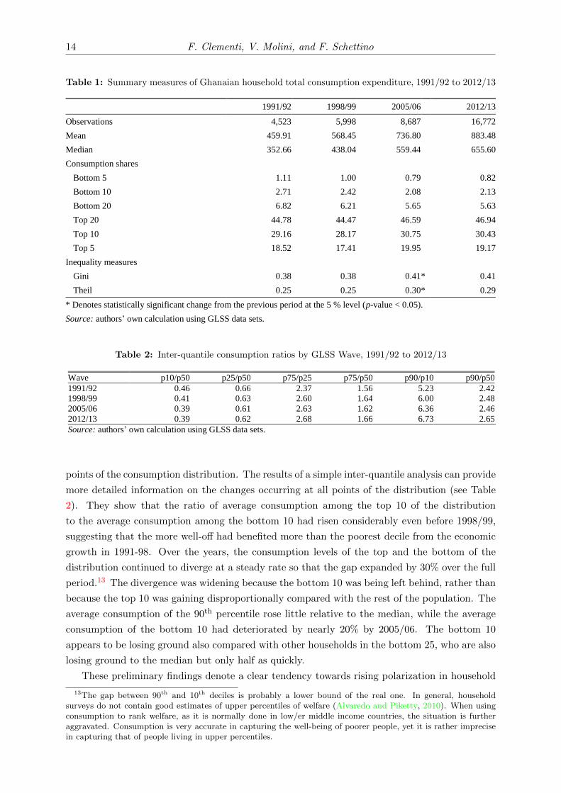
A summary of distributional statistics obtained from the GLSS data sets is given in Table 1.

Besides the growth of the real mean and median consumption expenditures, the most notable

feature is the picture that emerges across different indicators of inequality. The consumption

shares of the poorest percentiles of the population decreased between approximately 0.9 and 1.4%

a year in the period examined, in contrast to what is observed for the richest percentiles, whose

shares experienced average yearly increases of around 0.2%. Inequality in household consumption

was initially constant, but widened considerably between 1998/99 and 2005/06—a jump of about

7% in the Gini’s coefficient and 20% in the Theil’s index.12 Inequality has remained constant at

the higher level after 2005/06, but the trends in the shares of consumption of the bottom and

top quintiles have continued in the same direction.

However, the narrative about inequality is more nuanced than the summary measures suggest.

The summary measures of inequality analyzed above only partially capture the changes at various

10We use adult equivalent scales because also the official consumption, poverty and inequality figures are ex-pressed in adult equivalent terms.

11The price deflator differs across the ten regions in which Ghana is divided and within each region by urbanand rural areas.

12Running a simple t-test of the difference between Gini and Theil indices from the 1998/99 and 2005/06 samplesyields a p-value of around zero, which confirms the finding that points to increasing inequality over the 1998–2005period at any of the usual significance levels.

14 F. Clementi, V. Molini, and F. Schettino

Table 1: Summary measures of Ghanaian household total consumption expenditure, 1991/92 to 2012/13

1991/92 1998/99 2005/06 2012/13

Observations 4,523 5,998 8,687 16,772

Mean 459.91 568.45 736.80 883.48

Median 352.66 438.04 559.44 655.60

Consumption shares

Bottom 5 1.11 1.00 0.79 0.82

Bottom 10 2.71 2.42 2.08 2.13

Bottom 20 6.82 6.21 5.65 5.63

Top 20 44.78 44.47 46.59 46.94

Top 10 29.16 28.17 30.75 30.43

Top 5 18.52 17.41 19.95 19.17

Inequality measures

Gini 0.38 0.38 0.41 * 0.41

Theil 0.25 0.25 0.30 * 0.29

* Denotes statistically significant change from the previous period at the 5 % level (p-value < 0.05).

Source: authors’ own calculation using GLSS data sets.

Table 2: Inter-quantile consumption ratios by GLSS Wave, 1991/92 to 2012/13

Wave p10/p50 p25/p50 p75/p25 p75/p50 p90/p10 p90/p50

1991/92 0.46 0.66 2.37 1.56 5.23 2.42

1998/99 0.41 0.63 2.60 1.64 6.00 2.48

2005/06 0.39 0.61 2.63 1.62 6.36 2.46

2012/13 0.39 0.62 2.68 1.66 6.73 2.65

Source: authors’ own calculation using GLSS data sets.

Table 2: Inter-quantile consumption ratios by GLSS Wave, 1991/92 to 2012/13.

Wave p10/p50 p25/p50 p75/p25 p75/p50 p90/p10 p90/p50

1991/92 0.46 0.66 2.37 1.56 5.23 2.42

1998/99 0.41 0.63 2.60 1.64 6.00 2.48

2005/06 0.39 0.61 2.63 1.62 6.36 2.46

2012/13 0.39 0.62 2.68 1.66 6.73 2.65

Source: authors’ own calculation using GLSS data sets.

Table 2: Inter-quantile consumption ratios by GLSS Wave, 1991/92 to 2012/13.

Wave p10/p50 p25/p50 p75/p25 p75/p50 p90/p10 p90/p50

1991/92 0.46 0.66 2.37 1.56 5.23 2.42

1998/99 0.41 0.63 2.60 1.64 6.00 2.48

2005/06 0.39 0.61 2.63 1.62 6.36 2.46

2012/13 0.39 0.62 2.68 1.66 6.73 2.65

Source: authors’ own calculation using GLSS data sets.

points of the consumption distribution. The results of a simple inter-quantile analysis can provide

more detailed information on the changes occurring at all points of the distribution (see Table

2). They show that the ratio of average consumption among the top 10 of the distribution

to the average consumption among the bottom 10 had risen considerably even before 1998/99,

suggesting that the more well-off had benefited more than the poorest decile from the economic

growth in 1991-98. Over the years, the consumption levels of the top and the bottom of the

distribution continued to diverge at a steady rate so that the gap expanded by 30% over the full

period.13 The divergence was widening because the bottom 10 was being left behind, rather than

because the top 10 was gaining disproportionally compared with the rest of the population. The

average consumption of the 90th percentile rose little relative to the median, while the average

consumption of the bottom 10 had deteriorated by nearly 20% by 2005/06. The bottom 10

appears to be losing ground also compared with other households in the bottom 25, who are also

losing ground to the median but only half as quickly.

These preliminary findings denote a clear tendency towards rising polarization in household

13The gap between 90th and 10th deciles is probably a lower bound of the real one. In general, householdsurveys do not contain good estimates of upper percentiles of welfare (Alvaredo and Piketty, 2010). When usingconsumption to rank welfare, as it is normally done in low/er middle income countries, the situation is furtheraggravated. Consumption is very accurate in capturing the well-being of poorer people, yet it is rather imprecisein capturing that of people living in upper percentiles.

Polarization amidst poverty reduction: A case study of Nigeria and Ghana 15

consumption over the period. The notion of “polarization” commonly refers to the case where

there is a significant number of individuals who are very poor but there exists also a non-

negligible share of the population that is quite rich. Such a gap between the poor and the rich

implies evidently that there is no sizable middle class.14 As we will see later when applying

relative distribution methods, the distributional changes occurred between 1991/92 and 2012/13

hollowed out the middle of the Ghanaian household consumption distribution and increased the

concentration of households around the highest and lowest deciles, hence leading to an increase

of polarization.

5 Empirical results

5.1 Nigeria

5.1.1 Changes in the Nigerian household consumption distribution

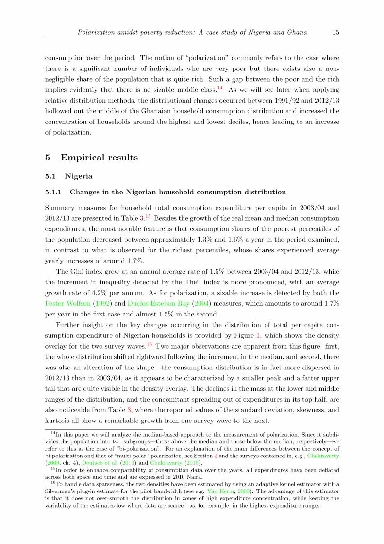
Summary measures for household total consumption expenditure per capita in 2003/04 and

2012/13 are presented in Table 3.15 Besides the growth of the real mean and median consumption

expenditures, the most notable feature is that consumption shares of the poorest percentiles of

the population decreased between approximately 1.3% and 1.6% a year in the period examined,

in contrast to what is observed for the richest percentiles, whose shares experienced average

yearly increases of around 1.7%.

The Gini index grew at an annual average rate of 1.5% between 2003/04 and 2012/13, while

the increment in inequality detected by the Theil index is more pronounced, with an average

growth rate of 4.2% per annum. As for polarization, a sizable increase is detected by both the

Foster-Wolfson (1992) and Duclos-Esteban-Ray (2004) measures, which amounts to around 1.7%

per year in the first case and almost 1.5% in the second.

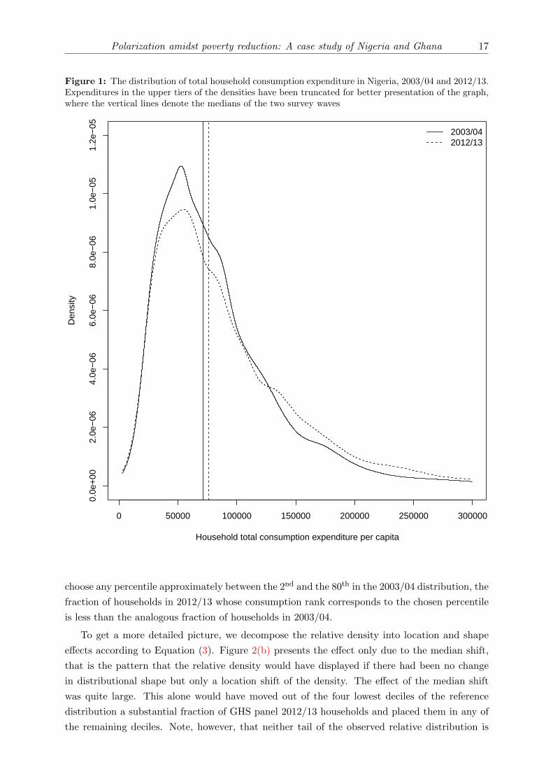
Further insight on the key changes occurring in the distribution of total per capita con-

sumption expenditure of Nigerian households is provided by Figure 1, which shows the density

overlay for the two survey waves.16 Two major observations are apparent from this figure: first,

the whole distribution shifted rightward following the increment in the median, and second, there

was also an alteration of the shape—the consumption distribution is in fact more dispersed in

2012/13 than in 2003/04, as it appears to be characterized by a smaller peak and a fatter upper

tail that are quite visible in the density overlay. The declines in the mass at the lower and middle

ranges of the distribution, and the concomitant spreading out of expenditures in its top half, are

also noticeable from Table 3, where the reported values of the standard deviation, skewness, and

kurtosis all show a remarkable growth from one survey wave to the next.

14In this paper we will analyze the median-based approach to the measurement of polarization. Since it subdi-vides the population into two subgroups—those above the median and those below the median, respectively—werefer to this as the case of “bi-polarization”. For an explanation of the main differences between the concept ofbi-polarization and that of “multi-polar” polarization, see Section 2 and the surveys contained in, e.g., Chakravarty(2009, ch. 4), Deutsch et al. (2013) and Chakravarty (2015).

15In order to enhance comparability of consumption data over the years, all expenditures have been deflatedacross both space and time and are expressed in 2010 Naira.

16To handle data sparseness, the two densities have been estimated by using an adaptive kernel estimator with aSilverman’s plug-in estimate for the pilot bandwidth (see e.g. Van Kerm, 2003). The advantage of this estimatoris that it does not over-smooth the distribution in zones of high expenditure concentration, while keeping thevariability of the estimates low where data are scarce—as, for example, in the highest expenditure ranges.

16 F. Clementi, V. Molini, and F. Schettino

Table 3: Summary measures of Nigerian household total consumption expenditure per capita

2003/04 2012/13

Mean 84,874 99,084

Median 71,168 76,193

Standard deviation 58,707 122,250

Skewness 2.48 39.32

Kurtosis 15.55 2,818.97

Consumption shares

Bottom 5% 1.05 0.93

Bottom 10% 2.64 2.29

Bottom 20% 6.90 5.97

Top 20% 41.14 45.45

Top 10% 25.43 29.52

Top 5% 15.35 18.97

Inequality measures

Gini 0.34 0.39

Theil 0.20 0.29

Polarization measuresa

Foster-Wolfson 0.30 0.35

Duclos-Esteban-Ray 0.21 0.24

Note: (a) the Duclos-Esteban-Ray index has been computed with the polarization sensitivity parameter α set at 0.5.

However, the graphical display above does not provide much information on the relative

impact that location and shape changes had on the differences in the two distributions at every

point of the expenditure scale. It also does not convey whether the upper and lower tails of

the consumption distribution were growing at the same rate and for what reasons (i.e. location

and/or shape driven). As already pointed out in Section 3, this is exactly what the relative

distribution method is particularly good at pulling out of the data.

We have chosen 2003/04 as the reference distribution throughout the analysis. It is important

to note that reversing the reference and comparison population designation will change the view

provided by the relative distribution graph and the displays of the estimated effects of location

and shape shifts, because these are defined in terms of the reference population scale. The

relative polarization indices, however, are symmetric, meaning that they are effectively invariant

to whether the 2003/04 or 2012/13 consumption distribution is chosen as the reference: in fact,

swapping the comparison and reference populations yields indices of the same magnitude and

opposite sign (e.g. Handcock and Morris, 1999, pp. 71–72, and Hao and Naiman, 2010, pp.

88–89). Thus, reversing the reference and comparison distributions designation will not alter our

findings in a substantive way—if not for the fact that polarization would now be analyzed in the

reverse direction of time.

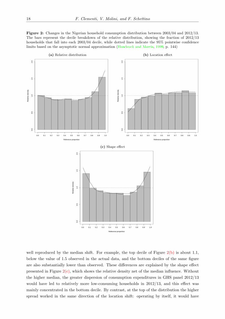
The relative density of total per capita consumption expenditure of Nigerian households

between 2003/04 and 2012/13 is examined in Figure 2(a).17 This plot shows the fraction of

households in 2012/13 that fall into each percentile of the 2003/04 distribution. Households in

the low and middle classes moved toward high and, to a less extent, lowest deciles. Indeed, if we

17The relative density function has been obtained by fitting a local polynomial to the estimated relative data.Throughout, we rely on the R statistical package reldist (Handcock, 2015) to implement the relative distributionmethod.

Polarization amidst poverty reduction: A case study of Nigeria and Ghana 17

Figure 1: The distribution of total household consumption expenditure in Nigeria, 2003/04 and 2012/13.Expenditures in the upper tiers of the densities have been truncated for better presentation of the graph,where the vertical lines denote the medians of the two survey waves

0 50000 100000 150000 200000 250000 300000

0.0e

+00

2.0e

−06

4.0e

−06

6.0e

−06

8.0e

−06

1.0e

−05

1.2e

−05

Household total consumption expenditure per capita

Den

sity

2003/042012/13

choose any percentile approximately between the 2nd and the 80th in the 2003/04 distribution, the

fraction of households in 2012/13 whose consumption rank corresponds to the chosen percentile

is less than the analogous fraction of households in 2003/04.

To get a more detailed picture, we decompose the relative density into location and shape

effects according to Equation (3). Figure 2(b) presents the effect only due to the median shift,

that is the pattern that the relative density would have displayed if there had been no change

in distributional shape but only a location shift of the density. The effect of the median shift

was quite large. This alone would have moved out of the four lowest deciles of the reference

distribution a substantial fraction of GHS panel 2012/13 households and placed them in any of

the remaining deciles. Note, however, that neither tail of the observed relative distribution is

18 F. Clementi, V. Molini, and F. Schettino

Figure 2: Changes in the Nigerian household consumption distribution between 2003/04 and 2012/13.The bars represent the decile breakdown of the relative distribution, showing the fraction of 2012/13households that fall into each 2003/04 decile, while dotted lines indicate the 95% pointwise confidencelimits based on the asymptotic normal approximation (Handcock and Morris, 1999, p. 144)

(a) Relative distribution

Reference proportion

Rel

ativ

e de

nsity

0.0

0.5

1.0

1.5

2.0

0.0 0.1 0.2 0.3 0.4 0.5 0.6 0.7 0.8 0.9 1.0

(b) Location effect

Reference proportion

Rel

ativ

e de

nsity

0.0

0.5

1.0

1.5

2.0

0.0 0.1 0.2 0.3 0.4 0.5 0.6 0.7 0.8 0.9 1.0

(c) Shape effect

Reference proportion

Rel

ativ

e de

nsity

0.0

0.5

1.0

1.5

2.0

0.0 0.1 0.2 0.3 0.4 0.5 0.6 0.7 0.8 0.9 1.0

well reproduced by the median shift. For example, the top decile of Figure 2(b) is about 1.1,

below the value of 1.5 observed in the actual data, and the bottom deciles of the same figure

are also substantially lower than observed. These differences are explained by the shape effect

presented in Figure 2(c), which shows the relative density net of the median influence. Without

the higher median, the greater dispersion of consumption expenditures in GHS panel 2012/13

would have led to relatively more low-consuming households in 2012/13, and this effect was

mainly concentrated in the bottom decile. By contrast, at the top of the distribution the higher

spread worked in the same direction of the location shift: operating by itself, it would have

Polarization amidst poverty reduction: A case study of Nigeria and Ghana 19

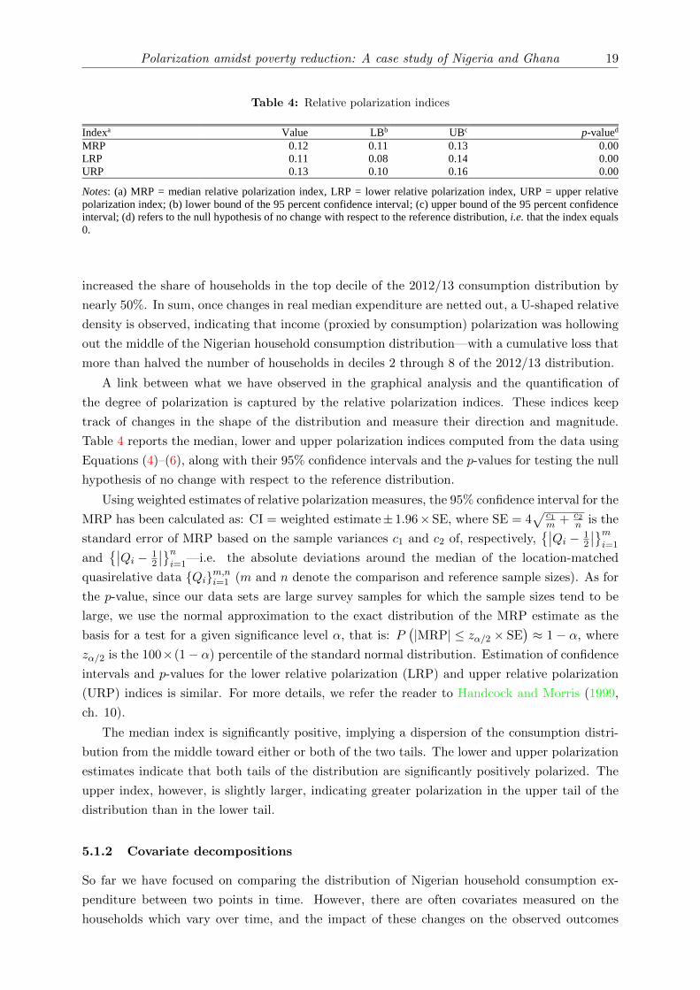
Table 4: Relative polarization indices

Indexa Value LBb UBc p-valued

MRP 0.12 0.11 0.13 0.00

LRP 0.11 0.08 0.14 0.00

URP 0.13 0.10 0.16 0.00

Notes: (a) MRP = median relative polarization index, LRP = lower relative polarization index, URP = upper relative

polarization index; (b) lower bound of the 95 percent confidence interval; (c) upper bound of the 95 percent confidence

interval; (d) refers to the null hypothesis of no change with respect to the reference distribution, i.e. that the index equals

0.

increased the share of households in the top decile of the 2012/13 consumption distribution by

nearly 50%. In sum, once changes in real median expenditure are netted out, a U-shaped relative

density is observed, indicating that income (proxied by consumption) polarization was hollowing

out the middle of the Nigerian household consumption distribution—with a cumulative loss that

more than halved the number of households in deciles 2 through 8 of the 2012/13 distribution.

A link between what we have observed in the graphical analysis and the quantification of

the degree of polarization is captured by the relative polarization indices. These indices keep

track of changes in the shape of the distribution and measure their direction and magnitude.

Table 4 reports the median, lower and upper polarization indices computed from the data using

Equations (4)–(6), along with their 95% confidence intervals and the p-values for testing the null

hypothesis of no change with respect to the reference distribution.

Using weighted estimates of relative polarization measures, the 95% confidence interval for the

MRP has been calculated as: CI = weighted estimate± 1.96×SE, where SE = 4√

c1m + c2

n is the

standard error of MRP based on the sample variances c1 and c2 of, respectively,{∣∣Qi − 1

2

∣∣}mi=1

and{∣∣Qi − 1

2

∣∣}ni=1

—i.e. the absolute deviations around the median of the location-matched

quasirelative data {Qi}m,ni=1 (m and n denote the comparison and reference sample sizes). As for

the p-value, since our data sets are large survey samples for which the sample sizes tend to be

large, we use the normal approximation to the exact distribution of the MRP estimate as the

basis for a test for a given significance level α, that is: P(|MRP| ≤ zα/2 × SE

)≈ 1 − α, where

zα/2 is the 100×(1− α) percentile of the standard normal distribution. Estimation of confidence

intervals and p-values for the lower relative polarization (LRP) and upper relative polarization

(URP) indices is similar. For more details, we refer the reader to Handcock and Morris (1999,

ch. 10).

The median index is significantly positive, implying a dispersion of the consumption distri-

bution from the middle toward either or both of the two tails. The lower and upper polarization

estimates indicate that both tails of the distribution are significantly positively polarized. The

upper index, however, is slightly larger, indicating greater polarization in the upper tail of the

distribution than in the lower tail.

5.1.2 Covariate decompositions

So far we have focused on comparing the distribution of Nigerian household consumption ex-

penditure between two points in time. However, there are often covariates measured on the

households which vary over time, and the impact of these changes on the observed outcomes

20 F. Clementi, V. Molini, and F. Schettino

could be of interest to economic policy and suggest possibilities worthy of consideration by its

designers. In the relative distribution setting, exploring the distributional impacts of changes in

a covariate requires that the relative distribution is adjusted for these changes using the methods

from Section 3.4. This makes it possible to separate the impacts of changes in the distribution of

the covariate (the “composition effect”) from changes in the conditional distributions of house-

hold consumption expenditure given the covariate levels (the “residual effect”). Our Nigerian

consumption microdata provide an opportunity to use this covariate adjustment technique as

they contain a large set of covariates describing various socio-demographic characteristics of the

respondents, household assets and characteristics of the dwelling. Here, the analysis is restricted

to the following covariates: sex of household head; literacy status of household head; zone; main

material used for floor; main source of drinking water; main cooking fuel; main toilet facility.

This selection was inspired both from previous poverty research—which advocates the inclu-

sion of covariates that change over time, but excluding those of them that are likely to change

markedly in the face of evolving economic conditions (e.g. Stifel and Christiaensen, 2007)—and

the fact that many of the covariates excluded from the analysis did not affect the statistical

significance of the predicting model used to impute the 2003/04 data.

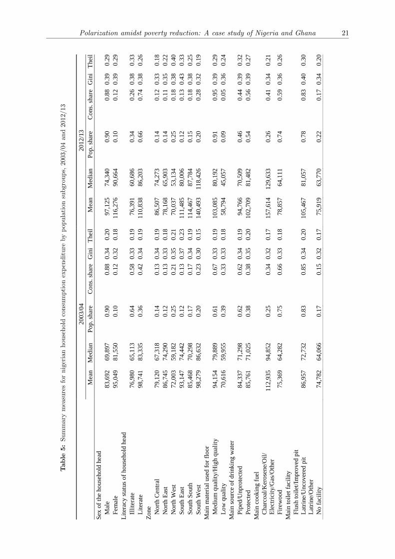
Summary statistics for the population subgroups defined by the levels of the covariates ana-

lyzed and the corresponding average percentage changes between 2003/04 and 2012/13 are given

in Tables 5 and 6. Both the mean and median consumption expenditures rose during the period

analyzed for many population subgroups—exceptions are represented by households headed by

illiterate individuals, households with inadequate housing infrastructures (such as unsafe water,

low quality flooring material, no toilet facility and firewood as the main cooking device) and

households living in the North East and North West zones of the country. At the same time,

apart from households in the North Central region, all groups experienced increasing inequality

according to both the Gini coefficient and the Theil index. Population and consumption shares

changed instead more heterogeneously, following patterns of increases and decreases with differ-

ent magnitudes over time. In particular, there appears to have been almost no change in the

proportion of male-headed households, while female-headed households declined somewhat. By

contrast, the fractions of households with a literate head and good quality housing infrastructures

(such as safe water, medium-high quality flooring material and non-firewood cooking devices)

grew considerably relative to their counterparts—households with no toilet facility, however, are

more common in 2012/13 than in 2003/04. Finally, the proportions of households that consist of

individuals living in the northern zones of the country increased between 2003/04 and 2012/13,

whereas households in the southern regions declined slightly.

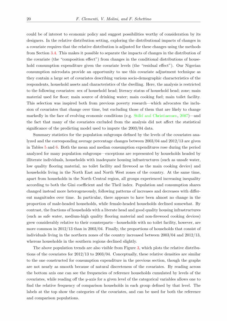
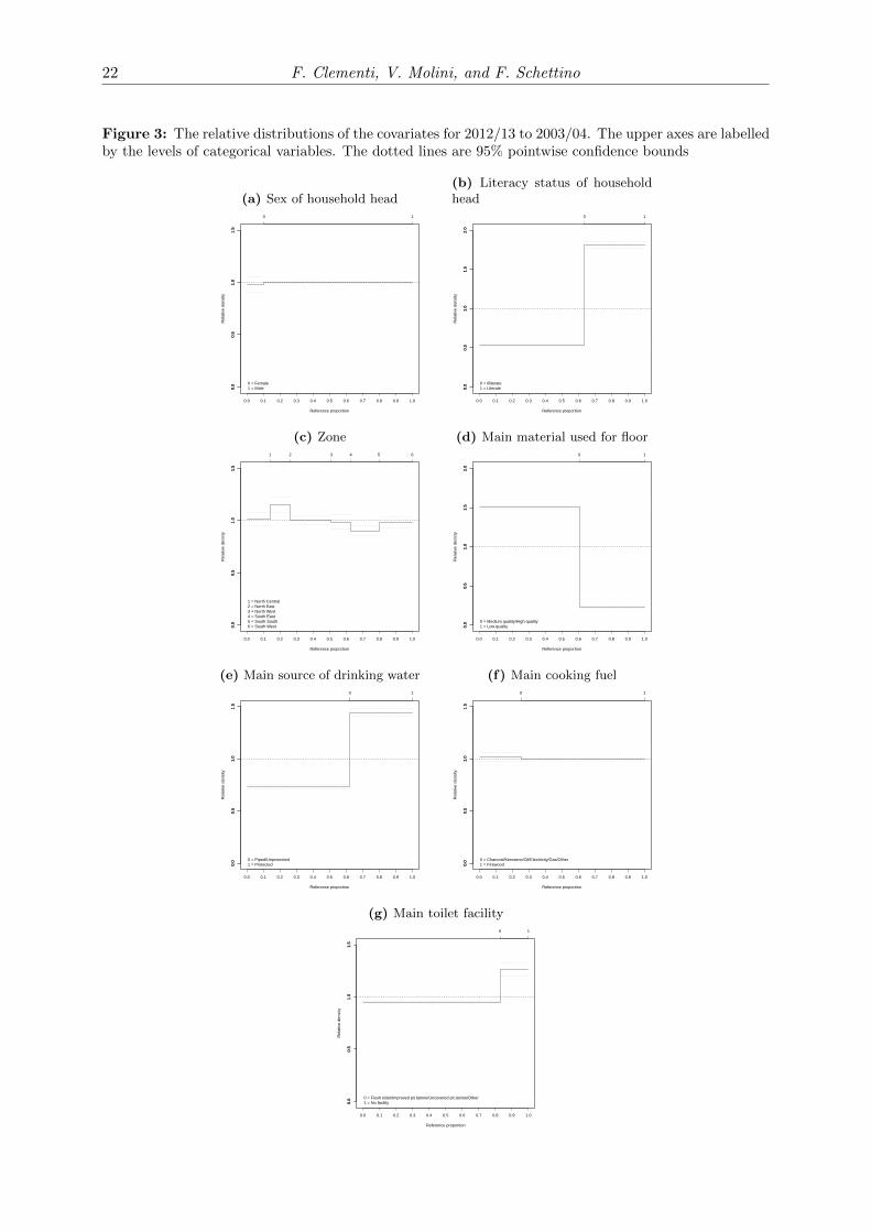
The above population trends are also visible from Figure 3, which plots the relative distribu-

tions of the covariates for 2012/13 to 2003/04. Conceptually, these relative densities are similar

to the one constructed for consumption expenditure in the previous section, though the graphs

are not nearly as smooth because of natural discreteness of the covariates. By reading across

the bottom axis one can see the frequencies of reference households cumulated by levels of the

covariates, while reading off the y-axis for a given level of the categorical variables allows one to

find the relative frequency of comparison households in each group defined by that level. The

labels at the top show the categories of the covariates, and can be used for both the reference

and comparison populations.

Polarization amidst poverty reduction: A case study of Nigeria and Ghana 21

Table

5:

Su

mm

ary

mea

sure

sfo

rn

iger

ian

hou

seh

old

con

sum

pti

on

exp

end

itu

reby

pop

ula

tion

sub

gro

up

s,2003/04

an

d2012/13

2

00

3/0

4

2

01

2/1

3

M

ean

M

edia

n

Po

p. sh

are

Co

ns.

shar

e

Gin

i T

hei

l

Mea

n

Med

ian

P

op

. sh

are

Co

ns.

shar

e

Gin

i T

hei

l

Sex

of

the

ho

use

ho

ld h

ead

M

ale

83

,692

6

9,8

97

0.9

0

0.8

8

0.3

4

0.2

0

97

,125

74

,340

0.9

0

0.8

8

0.3

9

0.2

9

F

em

ale

95

,049

8

1,5

50

0.1

0

0.1

2

0.3

2

0.1

8

11

6,2

76

90

,664

0.1

0

0.1

2

0.3

9

0.2

9

Lit

erac

y s

tatu

s o

f ho

use

ho

ld h

ead

I

llit

erat

e 7

6,9

80

6

5,1

13

0.6

4

0.5

8

0.3

3

0.1

9

76

,391

60

,686

0.3

4

0.2

6

0.3

8

0.3

3

L

iter

ate

98

,741

8

3,3

35

0.3

6

0.4

2

0.3

4

0.1

9

11

0,8

38

86

,203

0.6

6

0.7

4

0.3

8

0.2

6

Zo

ne

N

ort

h C

entr

al

79

,120

6

7,3

18

0.1

4

0.1

3

0.3

4

0.1

9

86

,507

74

,273

0.1

4

0.1

2

0.3

3

0.1

8

N

ort

h E

ast

86

,745

7

4,2

90

0.1

2

0.1

3

0.3

3

0.1

8

78

,168

65

,903

0.1

4

0.1

1

0.3

5

0.2

2

N

ort

h W

est

72

,003

5

9,1

82

0.2

5

0.2

1

0.3

5

0.2

1

70

,037

53

,134

0.2

5

0.1

8

0.3

8

0.4

0

S

outh

Eas

t 9

3,1

47

7

4,4

42

0.1

2

0.1

3

0.3

7

0.2

3

11

1,4

85

80

,006

0.1

2

0.1

3

0.4

3

0.3

3

S

outh

So

uth

8

5,4

68

7

0,2

98

0.1

7

0.1

7

0.3

4

0.1

9

11

4,4

67

87

,784

0.1

5

0.1

8

0.3

8

0.2

5

S

outh

Wes

t 9

8,2

79

8

6,6

32

0.2

0

0.2

3

0.3

0

0.1

5

14

0,4

93

11

8,4

26

0.2

0

0.2

8

0.3

2

0.1

9

Mai

n m

ater

ial

use

d f

or

flo

or

M

ediu

m q

ual

ity/H

igh q

ual

ity

9

4,1

54

7

9,8

89

0.6

1

0.6

7

0.3

3

0.1

9

10

3,0

85

80

,192

0.9

1

0.9

5

0.3

9

0.2

9

L

ow

quali

ty

70

,616

5

9,9

55

0.3

9

0.3

3

0.3

3

0.1

8

58

,794

45

,057

0.0

9

0.0

5

0.3

6

0.2

4

Mai

n s

ourc

e o

f d

rinkin

g w

ater

P

iped

/Unp

rote

cted

8

4,3

37

7

1,2

98

0.6

2

0.6

2

0.3

4

0.1

9

94

,766

70

,509

0.4

6

0.4

4

0.3

9

0.3

2

P

rote

cted

8

5,7

61

7

1,0

25

0.3

8

0.3

8

0.3

5

0.2

0

10

2,7

09

81

,482

0.5

4

0.5

6

0.3

9

0.2

7

Mai

n c

oo

kin

g f

uel

C

har

coal

/Ker

ose

ne/

Oil

/

E

lect

rici

ty/G

as/O

ther

1

12

,93

5

94

,852

0.2

5

0.3

4

0.3

2

0.1

7

15

7,6

14

12

9,6

33

0.2

6

0.4

1

0.3

4

0.2

1

F

irew

oo

d

75

,369

6

4,2

82

0.7

5

0.6

6

0.3

3

0.1

8

78

,857

64

,111

0.7

4

0.5

9

0.3

6

0.2

6

Mai

n t

oil

et f

acil

ity

F

lush

to

ilet

/Im

pro

ved

pit

L

atri

ne/

Unco

ver

ed p

it

L

atri

ne/

Oth

er

86

,957

7

2,7

32

0.8

3

0.8

5

0.3

4

0.2

0

10

5,4

67

81

,057

0.7

8

0.8

3

0.4

0

0.3

0

N

o f

acil

ity

7

4,7

82

64

,066

0.1

7

0.1

5

0.3

2

0.1

7

75

,919

63

,770

0.2

2

0.1

7

0.3

4

0.2

0

22 F. Clementi, V. Molini, and F. Schettino

Figure 3: The relative distributions of the covariates for 2012/13 to 2003/04. The upper axes are labelledby the levels of categorical variables. The dotted lines are 95% pointwise confidence bounds

(a) Sex of household head

0.0

0.5

1.0

1.5

Reference proportion

Rel

ativ

e de

nsity

0.0

0.5

1.0

1.5

0.0 0.1 0.2 0.3 0.4 0.5 0.6 0.7 0.8 0.9 1.0

0 1

0 = Female1 = Male

(b) Literacy status of householdhead

0.0

0.5

1.0

1.5

2.0

Reference proportion

Rel

ativ

e de

nsity

0.0

0.5

1.0

1.5

2.0

0.0 0.1 0.2 0.3 0.4 0.5 0.6 0.7 0.8 0.9 1.0

0 1

0 = Illiterate1 = Literate

(c) Zone

0.0

0.5

1.0

1.5

Reference proportion

Rel

ativ

e de

nsity

0.0

0.5

1.0

1.5

0.0 0.1 0.2 0.3 0.4 0.5 0.6 0.7 0.8 0.9 1.0

1 2 3 4 5 6

1 = North Central2 = North East3 = North West4 = South East5 = South South6 = South West

(d) Main material used for floor

0.0

0.5

1.0

1.5

2.0

Reference proportion

Rel

ativ

e de

nsity

0.0

0.5

1.0

1.5

2.0

0.0 0.1 0.2 0.3 0.4 0.5 0.6 0.7 0.8 0.9 1.0

0 1

0 = Medium quality/High quality1 = Low quality

(e) Main source of drinking water

0.0

0.5

1.0

1.5

Reference proportion

Rel

ativ

e de

nsity

0.0

0.5

1.0

1.5

0.0 0.1 0.2 0.3 0.4 0.5 0.6 0.7 0.8 0.9 1.0

0 1

0 = Piped/Unprotected1 = Protected

(f) Main cooking fuel

0.0

0.5

1.0

1.5

Reference proportion

Rel

ativ

e de

nsity

0.0

0.5

1.0

1.5

0.0 0.1 0.2 0.3 0.4 0.5 0.6 0.7 0.8 0.9 1.0

0 1

0 = Charcoal/Kerosene/Oil/Electricity/Gas/Other1 = Firewood

(g) Main toilet facility

0.0

0.5

1.0

1.5

Reference proportion

Rel

ativ

e de

nsity

0.0

0.5

1.0

1.5

0.0 0.1 0.2 0.3 0.4 0.5 0.6 0.7 0.8 0.9 1.0

0 1

0 = Flush toilet/Improved pit latrine/Uncovered pit latrine/Other1 = No facility

Polarization amidst poverty reduction: A case study of Nigeria and Ghana 23

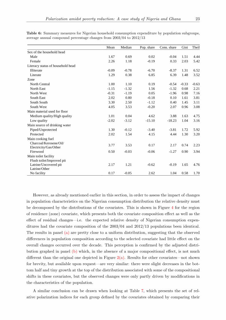
Table 6: Summary measures for Nigerian household consumption expenditure by population subgroups,average annual compound percentage changes from 2003/04 to 2012/13

Mean Median Pop. share Cons. share Gini Theil

Sex of the household head

Male 1.67 0.69 0.02 -0.04 1.51 4.44

Female 2.26 1.18 -0.19 0.33 2.03 5.42

Literacy status of household head

Illiterate -0.09 -0.78 -6.70 -8.37 1.31 6.52

Literate 1.29 0.38 6.85 6.39 1.48 3.52

Zone

North Central 1.00 1.10 0.19 -0.54 -0.33 -0.63

North East -1.15 -1.32 1.56 -1.32 0.68 2.21

North West -0.31 -1.19 0.05 -1.96 0.98 7.16

South East 2.02 0.80 -0.18 0.10 1.61 3.81

South South 3.30 2.50 -1.12 0.40 1.45 3.11

South West 4.05 3.53 -0.20 2.07 0.96 3.08

Main material used for floor

Medium quality/High quality 1.01 0.04 4.62 3.88 1.63 4.75

Low quality -2.02 -3.12 -15.10 -18.23 1.04 3.16

Main source of drinking water

Piped/Unprotected 1.30 -0.12 -3.40 -3.81 1.72 5.92

Protected 2.02 1.54 4.15 4.44 1.30 3.20

Main cooking fuel

Charcoal/Kerosene/Oil/

Electricity/Gas/Other 3.77 3.53 0.17 2.17 0.74 2.23

Firewood 0.50 -0.03 -0.06 -1.27 0.90 3.94

Main toilet facility

Flush toilet/Improved pit

Latrine/Uncovered pit

Latrine/Other

2.17 1.21 -0.62 -0.19 1.65 4.76

No facility 0.17 -0.05 2.62 1.04 0.58 1.70

However, as already mentioned earlier in this section, in order to assess the impact of changes

in population characteristics on the Nigerian consumption distribution the relative density must

be decomposed by the distributions of the covariates. This is shown in Figure 4 for the region

of residence (zone) covariate, which presents both the covariate composition effect as well as the

effect of residual changes—i.e. the expected relative density of Nigerian consumption expen-

ditures had the covariate composition of the 2003/04 and 2012/13 populations been identical.

The results in panel (a) are pretty close to a uniform distribution, suggesting that the observed

differences in population composition according to the selected covariate had little effect on the

overall changes occurred over the decade. This perception is confirmed by the adjusted distri-

bution graphed in panel (b) which, in the absence of a major compositional effect, is not much

different than the original one depicted in Figure 2(a). Results for other covariates—not shown

for brevity, but available upon request—are very similar: there were slight decreases in the bot-

tom half and tiny growth at the top of the distribution associated with some of the compositional

shifts in these covariates, but the observed changes were only partly driven by modifications in

the characteristics of the population.

A similar conclusion can be drawn when looking at Table 7, which presents the set of rel-

ative polarization indices for each group defined by the covariates obtained by comparing their

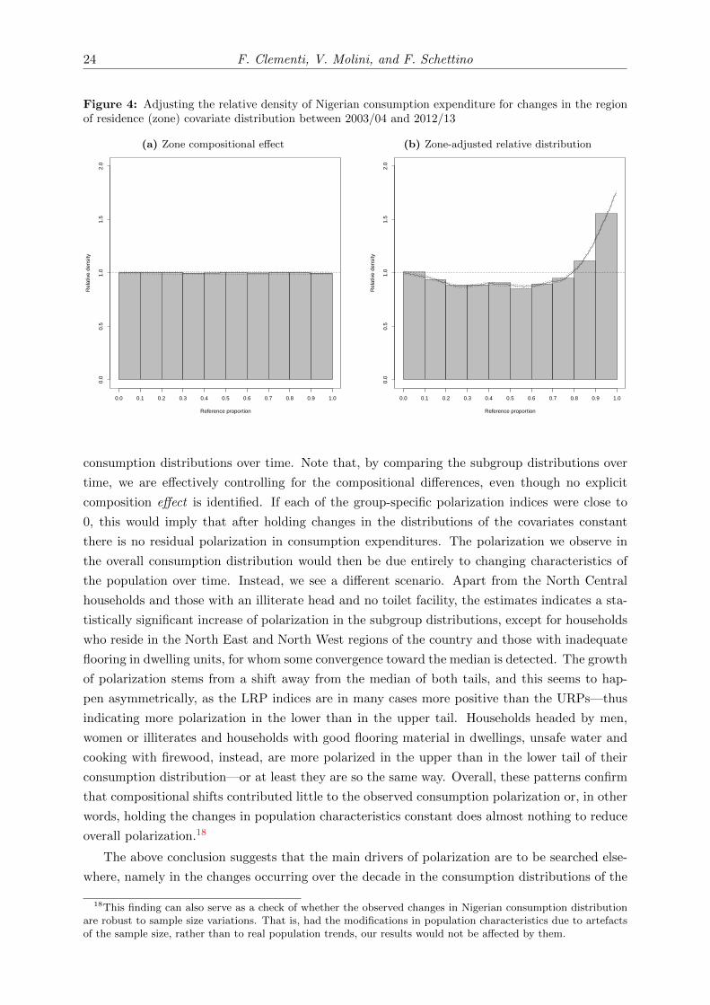
24 F. Clementi, V. Molini, and F. Schettino

Figure 4: Adjusting the relative density of Nigerian consumption expenditure for changes in the regionof residence (zone) covariate distribution between 2003/04 and 2012/13

(a) Zone compositional effect

Reference proportion

Rel

ativ

e de

nsity

0.0

0.5

1.0

1.5

2.0

0.0 0.1 0.2 0.3 0.4 0.5 0.6 0.7 0.8 0.9 1.0

(b) Zone-adjusted relative distribution

Reference proportion

Rel

ativ

e de

nsity

0.0

0.5

1.0

1.5

2.0

0.0 0.1 0.2 0.3 0.4 0.5 0.6 0.7 0.8 0.9 1.0

consumption distributions over time. Note that, by comparing the subgroup distributions over

time, we are effectively controlling for the compositional differences, even though no explicit

composition effect is identified. If each of the group-specific polarization indices were close to

0, this would imply that after holding changes in the distributions of the covariates constant

there is no residual polarization in consumption expenditures. The polarization we observe in

the overall consumption distribution would then be due entirely to changing characteristics of

the population over time. Instead, we see a different scenario. Apart from the North Central

households and those with an illiterate head and no toilet facility, the estimates indicates a sta-

tistically significant increase of polarization in the subgroup distributions, except for households

who reside in the North East and North West regions of the country and those with inadequate

flooring in dwelling units, for whom some convergence toward the median is detected. The growth

of polarization stems from a shift away from the median of both tails, and this seems to hap-

pen asymmetrically, as the LRP indices are in many cases more positive than the URPs—thus

indicating more polarization in the lower than in the upper tail. Households headed by men,

women or illiterates and households with good flooring material in dwellings, unsafe water and

cooking with firewood, instead, are more polarized in the upper than in the lower tail of their

consumption distribution—or at least they are so the same way. Overall, these patterns confirm

that compositional shifts contributed little to the observed consumption polarization or, in other

words, holding the changes in population characteristics constant does almost nothing to reduce

overall polarization.18

The above conclusion suggests that the main drivers of polarization are to be searched else-

where, namely in the changes occurring over the decade in the consumption distributions of the

18This finding can also serve as a check of whether the observed changes in Nigerian consumption distributionare robust to sample size variations. That is, had the modifications in population characteristics due to artefactsof the sample size, rather than to real population trends, our results would not be affected by them.

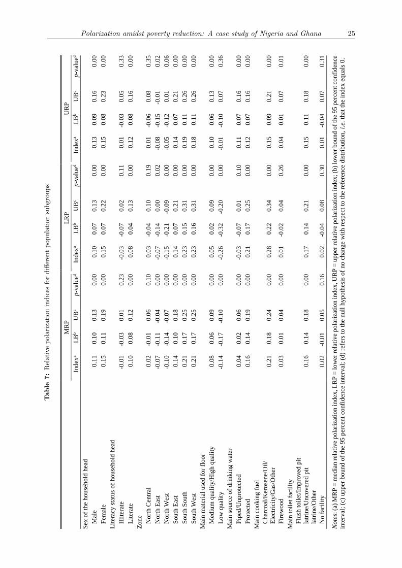
Polarization amidst poverty reduction: A case study of Nigeria and Ghana 25

Table

7:

Rel

ativ

ep

ola

riza

tion

ind

ices

for

diff

eren

tp

op

ula

tion

sub

gro

ups

M

RP

LR

P

U

RP

In

dex

a

LB

b

UB

c p

-val

ued

In

dex

a

LB

b

UB

c p

-val

ued

In

dex

a

LB

b

UB

c p

-val

ued

Sex

of

the

ho

use

ho

ld h

ead

M

ale

0.1

1

0.1

0

0.1

3

0.0

0

0.1

0

0.0

7

0.1

3

0.0

0

0.1

3

0.0

9

0.1

6

0.0

0

F

em

ale

0.1

5

0.1

1

0.1

9

0.0

0

0.1

5

0.0

7

0.2

2

0.0

0

0.1

5

0.0

8

0.2

3

0.0

0

Lit

erac

y s

tatu

s o

f ho

use

ho

ld h

ead

I

llit

erat

e -0

.01

-0

.03

0

.01

0.2

3

-0.0

3

-0.0

7

0.0

2

0.1

1

0.0

1

-0.0

3

0.0

5

0.3

3

L

iter

ate

0.1

0

0.0

8

0.1

2

0.0

0

0.0

8

0.0

4

0.1

3

0.0

0

0.1

2

0.0

8

0.1

6

0.0

0

Zo

ne

N

ort

h C

entr

al

0.0

2

-0.0

1

0.0

6

0.1

0

0.0

3

-0.0

4

0.1

0

0.1

9

0.0

1

-0.0

6

0.0

8

0.3

5

N

ort

h E

ast

-0.0

7

-0.1

1

-0.0

4

0.0

0

-0.0

7

-0.1

4

0.0

0

0.0

2

-0.0

8

-0.1

5

-0.0

1

0.0

2

N

ort

h W

est

-0.1

0

-0.1

4

-0.0

7

0.0

0

-0.1

5

-0.2

1

-0.0

9

0.0

0

-0.0

5

-0.1

2

0.0

1

0.0

6

S

outh

Eas

t 0

.14

0.1

0

0.1

8

0.0

0

0.1

4

0.0

7

0.2

1

0.0

0

0.1

4

0.0

7

0.2

1

0.0

0

S

outh

So

uth

0

.21

0.1

7

0.2

5

0.0

0

0.2

3

0.1

5

0.3

1

0.0

0

0.1

9

0.1

1

0.2

6

0.0

0

S

outh

Wes

t 0

.21

0.1

7

0.2

5

0.0

0

0.2

3

0.1

6

0.3

1

0.0

0

0.1

8

0.1

1

0.2

6

0.0

0

Mai

n m

ater

ial

use

d f

or

flo

or

M

ediu

m q

ual

ity/H

igh q

ual

ity

0

.08

0.0

6

0.0

9

0.0

0

0.0

5

0.0

2

0.0

9

0.0

0

0.1

0

0.0

6

0.1

3

0.0

0

L

ow

quali

ty

-0.1

4

-0.1

7

-0.1

0

0.0

0

-0.2

6

-0.3

2

-0.2

0

0.0

0

-0.0

1

-0.1

0

0.0

7

0.3

6

Mai

n s

ourc

e o

f d

rinkin

g w

ater

P

iped

/Unp

rote

cted

0

.04

0.0

2

0.0

6

0.0

0

-0.0

3

-0.0

7

0.0

1

0.1

0

0.1

1

0.0

7

0.1

6

0.0

0

P

rote

cted

0

.16

0.1

4

0.1

9

0.0

0

0.2

1

0.1

7

0.2

5

0.0

0

0.1

2

0.0

7

0.1

6

0.0

0

Mai

n c

oo

kin

g f

uel

C

har

coal

/Ker

ose

ne/

Oil

/

E

lect

rici

ty/G

as/O

ther

0

.21

0.1

8

0.2

4

0.0

0

0.2

8

0.2

2

0.3

4

0.0

0

0.1

5

0.0

9

0.2

1

0.0

0

F

irew

oo

d

0.0

3

0.0

1

0.0

4

0.0

0

0.0

1

-0.0

2

0.0

4

0.2

6

0.0

4

0.0

1

0.0

7

0.0

1

Mai

n t

oil

et f

acil

ity

F

lush

to

ilet

/Im

pro

ved

pit

l

atri

ne/

Unco

ver

ed p

it

l

atri

ne/

Oth

er

0.1

6

0.1

4

0.1

8

0.0

0

0.1

7

0.1

4

0.2

1

0.0

0

0.1

5

0.1

1

0.1

8

0.0

0

N

o f

acil

ity

0

.02

-0.0

1

0.0

5

0.1

6

0.0

2

-0.0

4

0.0

8

0.3

0

0.0

1

-0.0

4

0.0

7

0.3

1

Note

s: (

a) M

RP

= m

edia

n r

elat

ive

po

lari

zati

on ind

ex

, L

RP

= lo

wer

rel

ativ

e p

ola

riza

tio

n ind

ex, U

RP

= u

pp

er r

elat

ive p

ola

riza

tio

n ind

ex; (b

) lo

wer

bo

und

of

the

95

per

cent co

nfi

den

ce

inte

rval;

(c)

up

per

bo

und

of

the 9

5 p

erce

nt

confi

dence

inte

rval

; (d

) re

fers

to

the

null

hyp

oth

esis

of

no

change

wit

h r

esp

ect

to t

he

refe

rence

dis

trib

uti

on, i.e.

that

the

ind

ex e

quals

0.

26 F. Clementi, V. Molini, and F. Schettino

groups defined by the covariates. While the covariate adjustment technique identifies the impact

of changing population characteristics on the distribution of consumption expenditures, compar-

ing the groups defined by the covariates directly makes it possible to analyze the changes within

and between these groups’ consumption distributions. As already observed, most population

subgroups were both location-shifted (Tables 5 and 6) and more polarized (Table 7). To see

what impact these location and shape shifts in the subgroups’ distributions had on their relative

positions within the overall consumption distribution, we compare the changes in deciles of the

between-group relative distributions for 2003/04 and 2012/13 to the changes that would have

occurred if only the medians or shapes of the groups had changed. More specifically, for each

decile we decompose the absolute change:

g (C : R)− g (C0 : R0) , (19)

where g (C : R) and g (C0 : R0) denote respectively the relative density for comparison (C) to

reference (R) groups of the categorical variables in 2012/13 and 2003/04, into the marginal effect

of the median shift from the 2003/04 relative density:

g (C0L : R0L)− g (C0 : R0) , (20)

and those of the shape changes in the subgroups’ consumption distributions:

g (C0L : R)− g (C0L : R0L) , (21)

g (C : R)− g (C0L : R) , (22)

where R0L and C0L denote the distributions of the reference and comparison groups adjusted to

have the same median as 2012/13 but with the same shape as 2003/04.19 Summing up to the

total difference given by Equation (19), these effects form a complete decomposition and allow

us to determine what proportion of households were moved into or out of a decile of the overall

distribution by changes in relative median and group-specific shape.

The spatial distribution of household consumption expenditure definitely provided the most

attractive results. Figure 5 presents the decomposition for each of the six Nigerian macro-regions

as compared to the rest of the country. The solid bars show the total change by decile from

Equation (19), and each of the lines represents one of the three components in the decomposition

defined by Equations (20)–(22). We can see two ongoing distinctive patterns, both accentuating

polarization. In the South South and the South West, relative to the rest of the country, residents

tend to move out of the lower deciles of the distribution due to changes in relative median. More

precisely, had the location effect been the only one operating, we would have seen in both cases a

clear transition of Southeners from lower to upper deciles of the national distribution. However,

the shape effect of both regions moved in the opposite direction, partially offsetting the positive

impact of growth. Particularly in the lower deciles, the shape change is positive, indicating a

clear trend of lower polarization in these areas that goes in the opposite direction vis-a-vis the

19The decomposition follows the spirit of that presented in Bernhardt et al. (1995) and Handcock and Morris(1998, 1999), to whom we refer the reader for more details.

Polarization amidst poverty reduction: A case study of Nigeria and Ghana 27

national (residual) trend. This pattern is mirrored by what is going on in the upper deciles:

a location effect higher than in the rest of the country (especially in the South West) and an

accentuated tendency to upper polarization in both regions. For what concerns the North East

and the North West, the conflict-stricken areas, had the location effect been the only operating

force we would have seen a disproportionate increase of people in these regions occupying the

lower national deciles compared to the rest of the country—they basically lagged behind. The

increase of polarization in the rest of the country helped to offset this effect, filling the lower

deciles of households from other regions too, whereas for the rest of the distribution we observe in

practice a generalized decline of the relative position of these regions in the national distribution.

Finally, while the North Central improves relative to the rest of the country in lower deciles, the

South East comes to show a more articulated pattern of distributional change.

Results for the other covariates (not shown here but available upon request) looked as ex-

pected: compared to 2003/04, households with an illiterate head or not having good cooking

material, toilet, floor and safe water were all increasingly occupying the lower deciles of the

distribution, and the gap in terms of consumption with the rest was increasing. Instead, the

relative fraction of households headed by females in the upper deciles of the distribution was ris-

ing during the period, whereas male-headed households were moving into the deciles below the

median. In spite of the fact that Nigerian society is mainly patriarchal, where men have better

access to productive resources than women, the poor seems more among men than women.

5.2 Ghana

5.2.1 Changes in the Ghanaian consumption distribution

To introduce the results for Ghana, in Figure 6(a) we present two probability density functions of

the Ghanaian distribution of total consumption expenditure. The solid line is the distribution of

household consumption in 1991/92, taken as the baseline throughout the analysis. The density

drawn with the dotted line, which we will treat as the comparison, is the distribution in 2012/13.

Examining these two distributions, we see that the reference or 1991/92 distribution has a slight

right skewness, while the comparison distribution has a larger median and variance.

The relative density of total consumption expenditure of Ghanaian households between

1991/92 and 2012/13 is examined in Figure 6(b), showing the fraction of households in 2012/13

that fall into each decile of the 1991/92 distribution. The graph offers the immediate impression

that the proportion of households in the upper deciles increased dramatically throughout the

two decades, while the proportion in the bottom and around the middle declined. Indeed, if we

choose any decile between the first and the seventh in the 1991/92 distribution, the fraction of

households in 2012/13 whose consumption rank corresponds to the chosen decile is less than the

analogous fraction of households in 1991/92.

While the display of the relative distribution points to the dominant trend for the entire

period, the dominant trend may be masking some of the more subtle changes. To see these, we

decompose the relative density into location and shape effects. Figure 6(c) presents the effect

only due to the median shift that is the pattern that the relative density would have displayed

if there had been no change in distributional shape but only a location shift of the density.

The effect of the median shift was quite large. This alone would have virtually eliminated

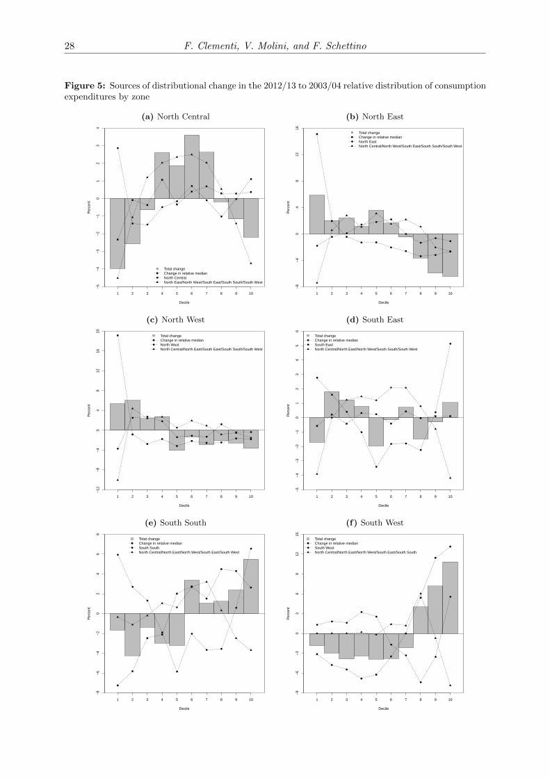
28 F. Clementi, V. Molini, and F. Schettino

Figure 5: Sources of distributional change in the 2012/13 to 2003/04 relative distribution of consumptionexpenditures by zone

(a) North Central

Decile

Per

cent

●

● ●

●

●

●

●

●

●

●

1 2 3 4 5 6 7 8 9 10

−5

−4

−3

−2

−1

01

23

4

●

Total changeChange in relative medianNorth CentralNorth East/North West/South East/South South/South West

(b) North East

Decile

Per

cent

●

●

●

●●

●

●

●

●

●

1 2 3 4 5 6 7 8 9 10−

8−

40

48

1216

●

Total changeChange in relative medianNorth EastNorth Central/North West/South East/South South/South West

(c) North West

Decile

Per

cent

●

● ●

●

●● ●

●

● ●

1 2 3 4 5 6 7 8 9 10

−12

−8

−4

04

812

1620

●

Total changeChange in relative medianNorth WestNorth Central/North East/South East/South South/South West

(d) South East

Decile

Per

cent

●

●

●

●

●

● ●

●

●

●

1 2 3 4 5 6 7 8 9 10

−5

−4

−3

−2

−1

01

23

45

6

●

Total changeChange in relative medianSouth EastNorth Central/North East/North West/South South/South West

(e) South South

Decile

Per

cent

●

●

●

●

●

●

● ●

●

●

1 2 3 4 5 6 7 8 9 10

−8

−6

−4

−2

02

46

8

●

Total changeChange in relative medianSouth SouthNorth Central/North East/North West/South East/South West

(f) South West

Decile

Per

cent

●

●●

●

●

●

●

●

●

●

1 2 3 4 5 6 7 8 9 10

−9

−6

−3

03

69

1215

●

Total changeChange in relative medianSouth WestNorth Central/North East/North West/South East/South South

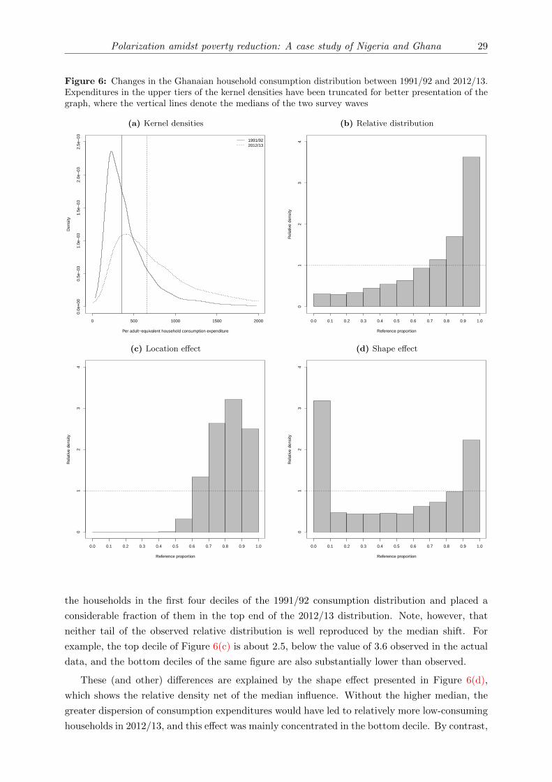
Polarization amidst poverty reduction: A case study of Nigeria and Ghana 29

Figure 6: Changes in the Ghanaian household consumption distribution between 1991/92 and 2012/13.Expenditures in the upper tiers of the kernel densities have been truncated for better presentation of thegraph, where the vertical lines denote the medians of the two survey waves

(a) Kernel densities

0 500 1000 1500 2000

Per adult−equivalent household consumption expenditure

Den

sity

0.0e

+00

0.5e

−03

1.0e

−03

1.5e

−03

2.0e

−03

2.5e

−03

1991/922012/13

(b) Relative distribution

Reference proportion

Rel

ativ

e de

nsity

01

23

4

0.0 0.1 0.2 0.3 0.4 0.5 0.6 0.7 0.8 0.9 1.0

(c) Location effect

Reference proportion

Rel

ativ

e de

nsity

01

23

4

0.0 0.1 0.2 0.3 0.4 0.5 0.6 0.7 0.8 0.9 1.0

(d) Shape effect

Reference proportion

Rel

ativ

e de

nsity

01

23

4

0.0 0.1 0.2 0.3 0.4 0.5 0.6 0.7 0.8 0.9 1.0

the households in the first four deciles of the 1991/92 consumption distribution and placed a

considerable fraction of them in the top end of the 2012/13 distribution. Note, however, that

neither tail of the observed relative distribution is well reproduced by the median shift. For

example, the top decile of Figure 6(c) is about 2.5, below the value of 3.6 observed in the actual

data, and the bottom deciles of the same figure are also substantially lower than observed.

These (and other) differences are explained by the shape effect presented in Figure 6(d),

which shows the relative density net of the median influence. Without the higher median, the

greater dispersion of consumption expenditures would have led to relatively more low-consuming

households in 2012/13, and this effect was mainly concentrated in the bottom decile. By contrast,

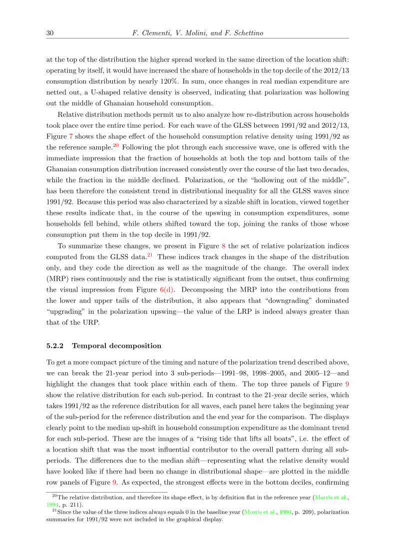
30 F. Clementi, V. Molini, and F. Schettino

at the top of the distribution the higher spread worked in the same direction of the location shift:

operating by itself, it would have increased the share of households in the top decile of the 2012/13

consumption distribution by nearly 120%. In sum, once changes in real median expenditure are

netted out, a U-shaped relative density is observed, indicating that polarization was hollowing

out the middle of Ghanaian household consumption.

Relative distribution methods permit us to also analyze how re-distribution across households

took place over the entire time period. For each wave of the GLSS between 1991/92 and 2012/13,

Figure 7 shows the shape effect of the household consumption relative density using 1991/92 as

the reference sample.20 Following the plot through each successive wave, one is offered with the

immediate impression that the fraction of households at both the top and bottom tails of the

Ghanaian consumption distribution increased consistently over the course of the last two decades,

while the fraction in the middle declined. Polarization, or the “hollowing out of the middle”,

has been therefore the consistent trend in distributional inequality for all the GLSS waves since

1991/92. Because this period was also characterized by a sizable shift in location, viewed together

these results indicate that, in the course of the upswing in consumption expenditures, some

households fell behind, while others shifted toward the top, joining the ranks of those whose

consumption put them in the top decile in 1991/92.

To summarize these changes, we present in Figure 8 the set of relative polarization indices

computed from the GLSS data.21 These indices track changes in the shape of the distribution

only, and they code the direction as well as the magnitude of the change. The overall index

(MRP) rises continuously and the rise is statistically significant from the outset, thus confirming

the visual impression from Figure 6(d). Decomposing the MRP into the contributions from

the lower and upper tails of the distribution, it also appears that “downgrading” dominated

“upgrading” in the polarization upswing—the value of the LRP is indeed always greater than

that of the URP.

5.2.2 Temporal decomposition

To get a more compact picture of the timing and nature of the polarization trend described above,

we can break the 21-year period into 3 sub-periods—1991–98, 1998–2005, and 2005–12—and

highlight the changes that took place within each of them. The top three panels of Figure 9

show the relative distribution for each sub-period. In contrast to the 21-year decile series, which

takes 1991/92 as the reference distribution for all waves, each panel here takes the beginning year

of the sub-period for the reference distribution and the end year for the comparison. The displays

clearly point to the median up-shift in household consumption expenditure as the dominant trend

for each sub-period. These are the images of a “rising tide that lifts all boats”, i.e. the effect of

a location shift that was the most influential contributor to the overall pattern during all sub-

periods. The differences due to the median shift—representing what the relative density would

have looked like if there had been no change in distributional shape—are plotted in the middle

row panels of Figure 9. As expected, the strongest effects were in the bottom deciles, confirming

20The relative distribution, and therefore its shape effect, is by definition flat in the reference year (Morris et al.,1994, p. 211).

21Since the value of the three indices always equals 0 in the baseline year (Morris et al., 1994, p. 209), polarizationsummaries for 1991/92 were not included in the graphical display.

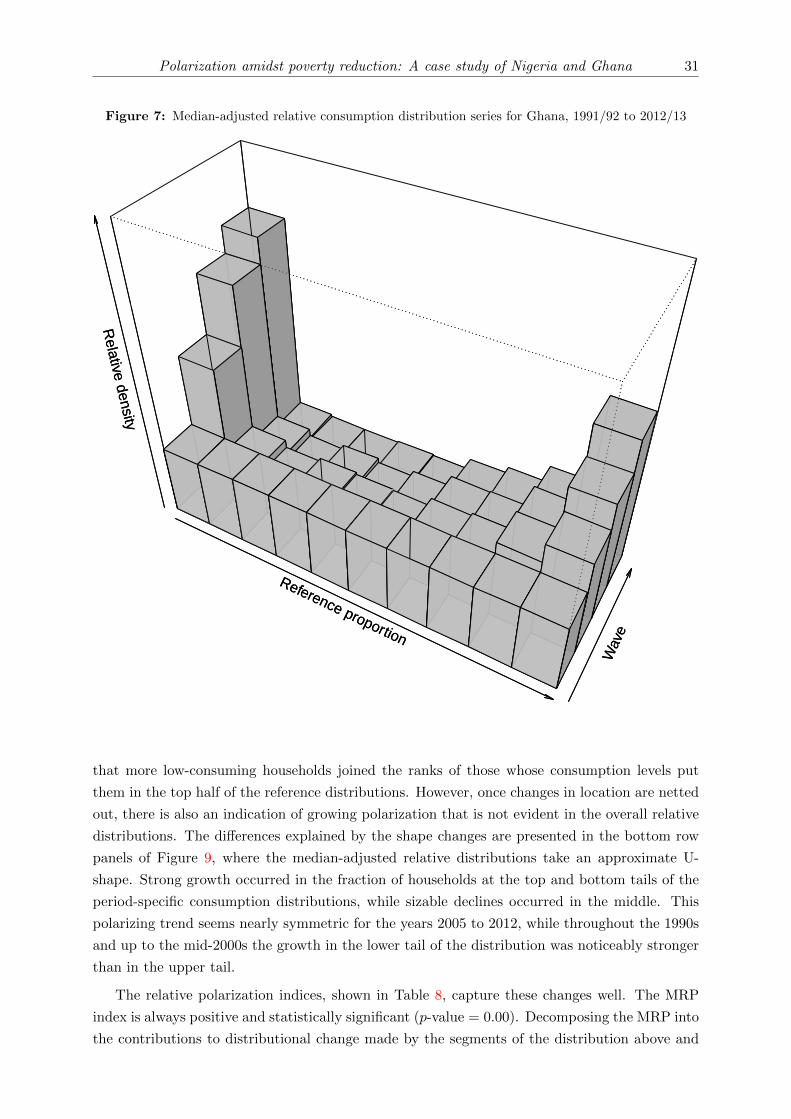
Polarization amidst poverty reduction: A case study of Nigeria and Ghana 31

Figure 7: Median-adjusted relative consumption distribution series for Ghana, 1991/92 to 2012/13

Reference proportion

Wav

e

Relative density

Reference proportion

Wav

e

Relative density

that more low-consuming households joined the ranks of those whose consumption levels put

them in the top half of the reference distributions. However, once changes in location are netted

out, there is also an indication of growing polarization that is not evident in the overall relative

distributions. The differences explained by the shape changes are presented in the bottom row

panels of Figure 9, where the median-adjusted relative distributions take an approximate U-

shape. Strong growth occurred in the fraction of households at the top and bottom tails of the

period-specific consumption distributions, while sizable declines occurred in the middle. This

polarizing trend seems nearly symmetric for the years 2005 to 2012, while throughout the 1990s

and up to the mid-2000s the growth in the lower tail of the distribution was noticeably stronger

than in the upper tail.

The relative polarization indices, shown in Table 8, capture these changes well. The MRP

index is always positive and statistically significant (p-value = 0.00). Decomposing the MRP into

the contributions to distributional change made by the segments of the distribution above and

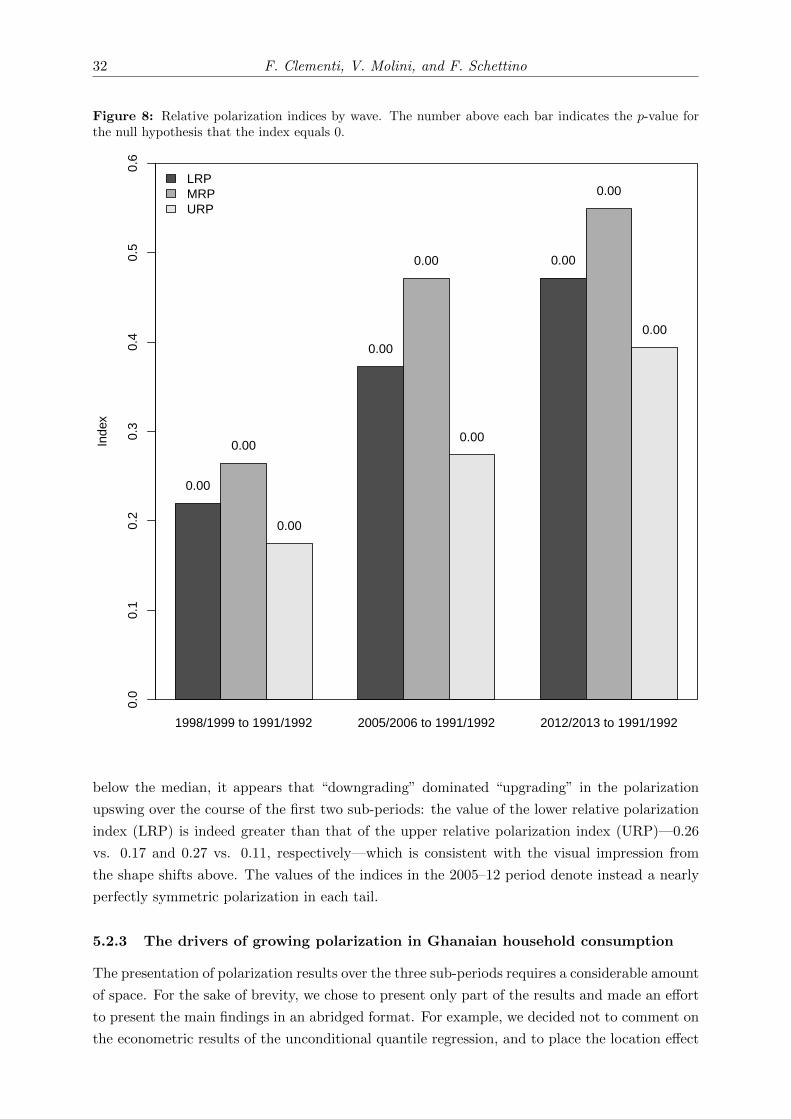
32 F. Clementi, V. Molini, and F. Schettino

Figure 8: Relative polarization indices by wave. The number above each bar indicates the p-value forthe null hypothesis that the index equals 0.

1998/1999 to 1991/1992 2005/2006 to 1991/1992 2012/2013 to 1991/1992

LRPMRPURP

Inde

x

0.0

0.1

0.2

0.3

0.4

0.5

0.6

0.00

0.00

0.00

0.00

0.00

0.00

0.00

0.00

0.00

below the median, it appears that “downgrading” dominated “upgrading” in the polarization

upswing over the course of the first two sub-periods: the value of the lower relative polarization

index (LRP) is indeed greater than that of the upper relative polarization index (URP)—0.26

vs. 0.17 and 0.27 vs. 0.11, respectively—which is consistent with the visual impression from

the shape shifts above. The values of the indices in the 2005–12 period denote instead a nearly

perfectly symmetric polarization in each tail.

5.2.3 The drivers of growing polarization in Ghanaian household consumption

The presentation of polarization results over the three sub-periods requires a considerable amount

of space. For the sake of brevity, we chose to present only part of the results and made an effort

to present the main findings in an abridged format. For example, we decided not to comment on

the econometric results of the unconditional quantile regression, and to place the location effect

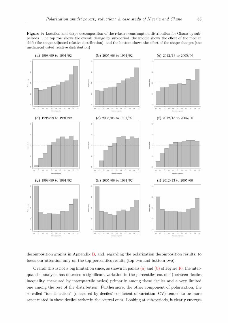
Polarization amidst poverty reduction: A case study of Nigeria and Ghana 33

Figure 9: Location and shape decomposition of the relative consumption distribution for Ghana by sub-periods. The top row shows the overall change by sub-period, the middle shows the effect of the medianshift (the shape-adjusted relative distribution), and the bottom shows the effect of the shape changes (themedian-adjusted relative distribution)

(a) 1998/99 to 1991/92

Reference proportion

Rel

ativ

e de

nsity

0.0

0.5

1.0

1.5

2.0

0.0 0.1 0.2 0.3 0.4 0.5 0.6 0.7 0.8 0.9 1.0

(b) 2005/06 to 1991/92

Reference proportion

Rel

ativ

e de

nsity

0.0

0.5

1.0

1.5

2.0

0.0 0.1 0.2 0.3 0.4 0.5 0.6 0.7 0.8 0.9 1.0

(c) 2012/13 to 2005/06

Reference proportion

Rel

ativ

e de

nsity

0.0

0.5

1.0

1.5

2.0

0.0 0.1 0.2 0.3 0.4 0.5 0.6 0.7 0.8 0.9 1.0

(d) 1998/99 to 1991/92

Reference proportion

Rel

ativ

e de

nsity

0.0

0.5

1.0

1.5

2.0

0.0 0.1 0.2 0.3 0.4 0.5 0.6 0.7 0.8 0.9 1.0

(e) 2005/06 to 1991/92

Reference proportion

Rel

ativ

e de

nsity

0.0

0.5

1.0

1.5

2.0

0.0 0.1 0.2 0.3 0.4 0.5 0.6 0.7 0.8 0.9 1.0

(f) 2012/13 to 2005/06

Reference proportion

Rel

ativ

e de

nsity

0.0

0.5

1.0

1.5

2.0

0.0 0.1 0.2 0.3 0.4 0.5 0.6 0.7 0.8 0.9 1.0

(g) 1998/99 to 1991/92

Reference proportion

Rel

ativ

e de

nsity

0.0

0.5

1.0

1.5

2.0

0.0 0.1 0.2 0.3 0.4 0.5 0.6 0.7 0.8 0.9 1.0

(h) 2005/06 to 1991/92

Reference proportion

Rel

ativ

e de

nsity

0.0

0.5

1.0

1.5

2.0

0.0 0.1 0.2 0.3 0.4 0.5 0.6 0.7 0.8 0.9 1.0

(i) 2012/13 to 2005/06

Reference proportion

Rel

ativ

e de

nsity

0.0

0.5

1.0

1.5

2.0

0.0 0.1 0.2 0.3 0.4 0.5 0.6 0.7 0.8 0.9 1.0

decomposition graphs in Appendix B, and, regarding the polarization decomposition results, to

focus our attention only on the top percentiles results (top two and bottom two).

Overall this is not a big limitation since, as shown in panels (a) and (b) of Figure 10, the inter-

quantile analysis has detected a significant variation in the percentiles cut-offs (between deciles

inequality, measured by interquartile ratios) primarily among these deciles and a very limited

one among the rest of the distribution. Furthermore, the other component of polarization, the

so-called “identification” (measured by deciles’ coefficient of variation, CV) tended to be more

accentuated in these deciles rather in the central ones. Looking at sub-periods, it clearly emerges

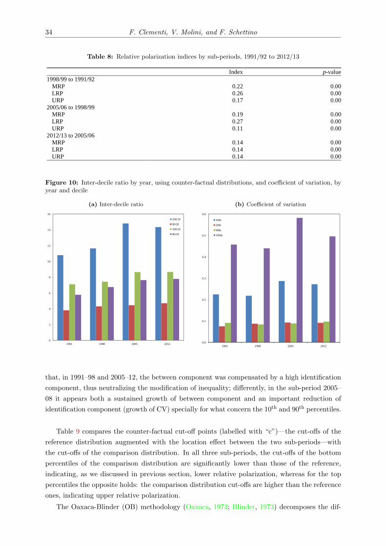
34 F. Clementi, V. Molini, and F. Schettino

Table 8: Relative polarization indices by sub-periods, 1991/92 to 2012/13

Index p-value

1998/99 to 1991/92

MRP 0.22 0.00

LRP 0.26 0.00

URP 0.17 0.00

2005/06 to 1998/99

MRP 0.19 0.00

LRP 0.27 0.00

URP 0.11 0.00

2012/13 to 2005/06

MRP 0.14 0.00

LRP 0.14 0.00

URP 0.14 0.00

Source: authors’ own calculation using GLSS data sets.

Figure 10: Inter-decile ratio by year, using counter-factual distributions, and coefficient of variation, byyear and decile

(a) Inter-decile ratio

0

2

4

6

8

10

12

14

16

1991 1998 2005 2012

100/10

90/20

100/20

90/10

(b) Coefficient of variation

0.0

0.1

0.2

0.3

0.4

0.5

0.6

1991 1998 2005 2012

10th

20th

90th

100th

that, in 1991–98 and 2005–12, the between component was compensated by a high identification

component, thus neutralizing the modification of inequality; differently, in the sub-period 2005–

08 it appears both a sustained growth of between component and an important reduction of

identification component (growth of CV) specially for what concern the 10th and 90th percentiles.

Table 9 compares the counter-factual cut-off points (labelled with “c”)—the cut-offs of the

reference distribution augmented with the location effect between the two sub-periods—with

the cut-offs of the comparison distribution. In all three sub-periods, the cut-offs of the bottom

percentiles of the comparison distribution are significantly lower than those of the reference,

indicating, as we discussed in previous section, lower relative polarization, whereas for the top

percentiles the opposite holds: the comparison distribution cut-offs are higher than the reference

ones, indicating upper relative polarization.

The Oaxaca-Blinder (OB) methodology (Oaxaca, 1973; Blinder, 1973) decomposes the dif-

Polarization amidst poverty reduction: A case study of Nigeria and Ghana 35

Table 9: Counterfactual reference cut-offs vs. comparison cut-offs: by deciles and sub-periods

Decile 1991c 1998 1998c 2005 2005c 2012

1st 248.74 181.03 302.43 216.83 312.99 258.36

2nd

296.69 246.72 368.12 304.00 400.17 357.47

8th

704.60 803.14 924.54 1,011.40 1,107.56 1,242.97

9th

940.64 1,084.86 1,206.26 1,377.14 1,473.31 1,738.20

Source: authors’ own calculation using GLSS data sets.

ference between cut-offs into that part that is due to group differences in the magnitudes of the

determinants (endowments effect) of consumption, on the one hand, and group differences in

the effects of these determinants (coefficients effect), on the other. Coefficient and endowment

variations are aggregated by groups of variables: primary, secondary and tertiary education are

grouped into the education attainment group, private, public and self- employment of household

head are grouped into employment category, the infrastructure index captures the access to ba-

sic services,22 urbanization and residence in regions other than Upper East (urban and regional

dummies having as baseline Upper East) and household structure (household size and all other

household characteristics). The interaction term and the constant are also included so that the

sum of all decomposition elements adds up to the total differences between cut-offs. Below any

decomposition graph, we present a table summarizing the main variable trends for upper and

lower polarization.

Recalling previous section results regarding 1991–98 sub-period, the polarization increased

as testified by the shifts leftward and rightward of the lower and upper cut-offs, respectively.

The polarization decomposition shows how the combined effect of household composition, in-

frastructure index and the constant increased the lower polarization while location effects and

education tended to reduce the effect. On the upper deciles nearly the same variables played a

pro-polarization role (Figure 11). Between 1991 and 1998 growth concentrated in urban areas

and in few regions on the Coast or in the immediate inland (Ashanti region) among households

with relatively higher levels of education and with access to a number of basic infrastructures.

This group of households occupying the top two deciles of the distribution distances itself from

the rest of other groups determining an increase in the upper polarization.

The 1998–2005 sub-period sees polarization growing. In this decade, Ghana experienced a

boom in cocoa production and exports. The cocoa boom generated, in the western and coastal

areas, a high demand for the workforce, but also for capital and infrastructure, and the skills of

the workforce and the rise in revenues even at lower levels translated into a higher demand for

capital, infrastructure and skills (Molini and Paci, 2015). These resources were relatively scarce,

and the price effect and variation in returns was, thus, substantial. In these areas, the cocoa

boom had a positive impact on poverty, but did not benefit everybody equally.

The drivers of polarization, both upper and lower, were very similar (Figure 12). Household

characteristics, educational attainment and basic infrastructures all tended to have pro-inequality

outcome and increased the tails size of the 2005 distribution, indeed more polarization. It is worth

22The infrastructure index is obtained by combining four variables through principal component analysis: accessto protected water, access to electricity, access to protected sanitation, and access to safe sources of cooking.

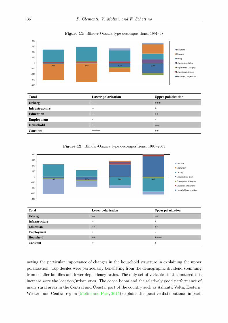
36 F. Clementi, V. Molini, and F. Schettino

Figure 11: Blinder-Oaxaca type decompositions, 1991–98

Total Lower polarization Upper polarization

Urbreg --- +++

Infrastructure + +

Education -- ++

Employment - -

Household + ----

Constant ++++ ++

-400

-300

-200

-100

0

100

200

300

400

10th 20th 80th 90th

Interaction

Constant

Urbreg

Infrastructure index

Employment Category

Education attainment

Household composition

Figure 12: Blinder-Oaxaca type decompositions, 1998–2005

Total Lower polarization Upper polarization

Urbreg --- ---

Infrastructure + +

Education ++ ++

Employment + -

Household ++ ++++

Constant + +

-400

-300

-200

-100

0

100

200

300

400

10th 20th 80th 90th

constant

Interaction

Urbreg

Infrastructure index

Employment Category

Education attainment

Household composition

noting the particular importance of changes in the household structure in explaining the upper

polarization. Top deciles were particularly benefitting from the demographic dividend stemming

from smaller families and lower dependency ratios. The only set of variables that countered this

increase were the location/urban ones. The cocoa boom and the relatively good performance of

many rural areas in the Central and Coastal part of the country such as Ashanti, Volta, Eastern,

Western and Central region (Molini and Paci, 2015) explains this positive distributional impact.

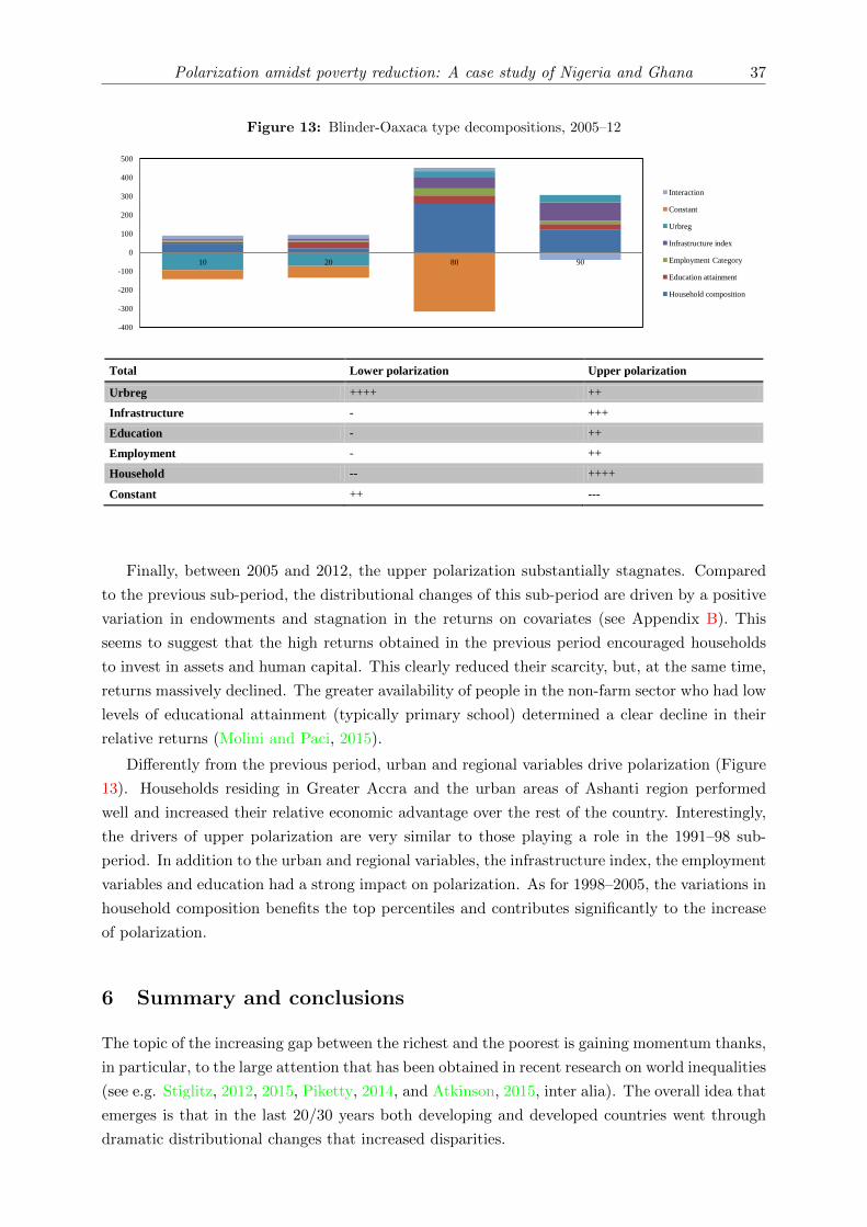
Polarization amidst poverty reduction: A case study of Nigeria and Ghana 37

Figure 13: Blinder-Oaxaca type decompositions, 2005–12

Total Lower polarization Upper polarization

Urbreg ++++ ++

Infrastructure - +++

Education - ++

Employment - ++

Household -- ++++

Constant ++ ---

-400

-300

-200

-100

0

100

200

300

400

500

10 20 80 90

Interaction

Constant

Urbreg

Infrastructure index

Employment Category

Education attainment

Household composition

Finally, between 2005 and 2012, the upper polarization substantially stagnates. Compared

to the previous sub-period, the distributional changes of this sub-period are driven by a positive

variation in endowments and stagnation in the returns on covariates (see Appendix B). This

seems to suggest that the high returns obtained in the previous period encouraged households

to invest in assets and human capital. This clearly reduced their scarcity, but, at the same time,

returns massively declined. The greater availability of people in the non-farm sector who had low

levels of educational attainment (typically primary school) determined a clear decline in their

relative returns (Molini and Paci, 2015).

Differently from the previous period, urban and regional variables drive polarization (Figure

13). Households residing in Greater Accra and the urban areas of Ashanti region performed

well and increased their relative economic advantage over the rest of the country. Interestingly,

the drivers of upper polarization are very similar to those playing a role in the 1991–98 sub-

period. In addition to the urban and regional variables, the infrastructure index, the employment

variables and education had a strong impact on polarization. As for 1998–2005, the variations in

household composition benefits the top percentiles and contributes significantly to the increase

of polarization.

6 Summary and conclusions

The topic of the increasing gap between the richest and the poorest is gaining momentum thanks,

in particular, to the large attention that has been obtained in recent research on world inequalities

(see e.g. Stiglitz, 2012, 2015, Piketty, 2014, and Atkinson, 2015, inter alia). The overall idea that

emerges is that in the last 20/30 years both developing and developed countries went through

dramatic distributional changes that increased disparities.

38 F. Clementi, V. Molini, and F. Schettino

Specifically with regard to Sub-Saharan Africa, there have been two different narratives in

the last two decades. The first paints a picture of an emerging continent where middle classes are

expanding and prosperity is reaching large swaths of the population (African Development Bank,

2011; Fine et al., 2012). The other narrative acknowledges the relatively robust growth in the

past two decades, but points to slow reduction in poverty. According to this second narrative,

the lack of faster reduction in poverty may be due, in part, to increasing disparities.

Nigeria, the most populous country in the African continent, has been enjoying a stable and

sustained growth for over a decade since 2003. Yet despite this, the outcomes in terms of poverty

reduction have not been satisfactory: while poverty seems to have declined in the coastal South

and around the Federal Capital, Abuja, a large belt of North-Eastern states have experienced a

clear stagnation in poverty reduction.

Over the last decade, Nigeria has also been going through significant changes in the distribu-

tion of economic resources that generated mainly, but not exclusively, an increase in polarization.

In income-polarized societies people cluster around group means and tend to be far from the

mean/median of the overall distribution, which results in the inability of the middle class to

consolidate its position. This has several economic consequences for a country, but may also be

the underlying cause of growing political instability seen in recent years in many middle income

countries.

Studies of polarization in Nigeria are few and have tackled the topic with a narrow lense.

This paper contributes to our understanding of polarization in Nigeria by using an approach that

improves upon previous studies in several ways. First, it considers a longer time horizon—close

to a decade—which allows for major changes in welfare distributions to emerge. Second, it tack-

les a major deficiency—lack of comparability of the available data in Nigeria—by making use

of survey-to-survey estimation techniques (Elbers et al., 2003) to achieve comparability of the

distributions of interest. Finally, and most importantly, it employs the “relative distribution”

approach Handcock and Morris (1998, 1999) to analyze changes in the Nigerian household con-

sumption distribution in the considered period. The novelty of this method consists in providing

a non-parametric framework for taking into account all of the distributional differences that

could arise in the comparison of distributions over time and space. In this way, we are able to

summarize multiple features of the expenditure distribution that would not be detected easily

from a comparison of standard measures of inequality and polarization.

The analysis reveals significant changes in the consumption distribution. We find a clear

rise in polarization, meaning that the distributional movements observed between 2003/04 and

2012/13 hollowed out the middle of the Nigerian household consumption distribution and in-

creased concentration of the mass toward higher and lower deciles.

This pattern of distributional change, however, is not entirely homogeneous within the coun-

try, but varies from zone to zone. Through covariates analysis, controlling for spatial character-

istics of household head, we show that in the South (South-West and South-South) lower deciles

tend to be emptied relative to the rest of the country, confirming the tendency for households

from these zones to contribute to upper polarization. In the North-West and in the conflict-

stricken North-East, we see the opposite. The overall impact was a generalized hollowing out

of the center and a further accentuation of the North-South divide already characterizing the

country.

Polarization amidst poverty reduction: A case study of Nigeria and Ghana 39

Understanding the political and economic consequences of these sharp distributional changes

is beyond the scope of this paper. However, polarization is increasingly becoming a concern in

many developing countries. Recent episodes in Brazil, Egypt and Turkey suggest the existence

of a link between polarization and conflict, yet so far no relevant empirical evidence has been

produced to underpin the existing theoretical models (Esteban and Schneider, 2008). Nigeria is

clearly an ideal candidate for such analysis, and our future research will be directed in under-

standing how existing conflicts in Nigerian society can be interpreted and linked to the patterns

of polarization.

The case of Ghana also presents interesting specificities. Since 1991, poverty had declined

very fast, inequality has not increased dramatically and yet the country has seen a rapid surge

in polarization. The relative distribution analysis suggest that the distributional changes hol-

lowed out the middle of the Ghanaian household consumption distribution and increased the

concentration of households around the highest and lowest deciles.

Using a novel methodology to identify the drivers of distributional changes and quantify their

impact on the welfare distribution, our results indicate that, although there is some heterogeneity

across the various sub-periods in particular in terms of magnitude, household characteristics,

educational attainment and access to basic infrastructures all tended to increase over time the

size of the upper and lower tails of the consumption distribution and as a consequence the

degree of polarization. Urban/rural and regional variables started to have a strong impact on

polarization only in the last decade; households residing in Greater Accra and the urban areas

of Ashanti region performed well and increased their relative economic advantage over the rest

of the country.

From a policy perspective, the pro-polarization impact of variables that tend to change

slowly over time is of particular concern. It is very unlikely that policy makers can find a quick

fix to the problem and any intervention will produce results only in the long run. This implies

that the country needs to start now to develop a strategy that, if not able to immediately

reverse polarization, at least can mitigate its impact. The creation of a modern social protection

system, the expansion in the access to basic services, the continued effort to expand primary and

secondary education are all interventions that can pay off and help the country to maintain its

social cohesion.

40 F. Clementi, V. Molini, and F. Schettino

References

African Development Bank. Annual Report. Statistics Department of the African Development

Bank Group, 2011. Available at http://www.afdb.org/knowledge/publications/annual-

report/annual-report-2011/.

F. C. Ahmed, C. Dorji, S. Takamatsu, and N. Yoshida. Hybrid Survey to

Improve the Reliability of Poverty Statistics in a Cost-Effective Manner. Pol-

icy Research Working Paper 6909, World Bank Group, Washington, DC, 2014.

Available at http://documents.worldbank.org/curated/en/2014/06/19641283/hybrid-

survey-improve-reliability-poverty-statistics-cost-effective-manner.

B. E. Aigbokhan. Poverty, Growth and Inequality in Nigeria: A Case Study. AERC

Research Paper 102, African Economic Research Consortium, Nairobi, 2000. Available

at http://www.aercafrica.org/index.php/publications/view_document/112-poverty-

growth-and-inequality-in-nigeria-a-case-study.

A. S. Alderson and K. Doran. Global Inequality, Within-Nation Inequality, and the Changing

Distribution of Income in Seven Transitional and Middle-Income Societies. In C. Suter, ed-

itor, Inequality Beyond Globalization: Economic Changes, Social Transformations, and the

Dynamics of Inequality, pages 183–200. Transaction Publishers, New Brunswick, NJ, 2011.

A. S. Alderson and K. Doran. How Has Income Inequality Grown? The Reshaping of the In-

come Distribution in LIS Countries. In J. C. Gornick and M. Jantti, editors, Income Inequality:

Economic Disparities and the Middle Class in Affluent Countries, pages 51–74. Stanford Uni-

versity Press, Stanford, CA, 2013.

A. S. Alderson, J. Beckfield, and F. Nielsen. Exactly How Has Income Inequality Changed?

Patterns of Distributional Change in Core Societies. International Journal of Comparative

Sociology, 46:405–423, 2005.

F. Alvaredo and T. Piketty. The Dynamics of Income Concentration in Developed and Developing

Countries: A View from the Top. In L. F. Lopez-Calva and N. Lustig, editors, Declining

Inequality in Latin America: A Decade of Progress?, pages 72–99. Brookings Institution Press,

Baltimore, MD, 2010.

G. Anderson, O. Linton, and T. W. Leo. A Polarization-Cohesion Perspective on Cross-Country

Convergence. Journal of Economic Growth, 17:49–69, 2012.

A. Araar. On the Decomposition of Polarization Indices: Illustrations with Chinese and Nigerian

Household Surveys. Working Paper 08-06, Centre Interuniversitaire sur le Risque, les Politiques

Economiques et l’Emploi (CIRPEE), Montreal, 2008. Available at http://www.cirpee.org/

fileadmin/documents/Cahiers_2008/CIRPEE08-06.pdf.

A. B. Atkinson. Inequality: What Can Be Done? Harvard University Press, Cambridge, MA,

2015.

Polarization amidst poverty reduction: A case study of Nigeria and Ghana 41

T. T. Awoyemi and A. Araar. Explaining Polarization and its Dimensions in Nigeria: A DER De-

composition Approach. Paper prepared for the 14nd Annual Conference on Econometric Mod-

elling for Africa, Abuja, Nigeria, July 8–10, 2009. Available at http://www.africametrics.

org/documents/conference09/papers/Awoyemi_Araar.pdf.

T. T. Awoyemi, I. B. Oluwatayo, and A. Oluwakemi. Inequality, Polarization and Poverty in

Nigeria. Working Paper 2010-04, Partnership for Economic Policy (PEP), Nairobi, 2010.

Available at http://www.pep-net.org/communications/working-papers/.

P. Backiny-Yetna, D. Steele, and I. Y. Djima. The Impact of Household Food Consump-

tion Data Collection Methods on Poverty and Inequality Measures in Niger. Policy

Research Working Paper 7090, World Bank Gorup, Washington, DC, 2014. Available at

http://documents.worldbank.org/curated/en/2014/11/20353374/impact-household-

food-consumption-data-collection-methods-poverty-inequality-measures-niger.

K. Beegle, J. De Weerdt, J. Friedman, and J. Gibson. Methods of Household Consump-

tion Measurement through Surveys: Experimental Results from Tanzania. Policy Re-

search Working Paper 5501, World Bank Group, Washington, DC, 2010. Available at

http://documents.worldbank.org/curated/en/2010/12/13233228/methods-household-

consumption-measurement-through-surveys-experimental-results-tanzania.

A. Bernhardt, M. Morris, and M. S. Handcock. Women’s Gains or Mens Losses? A Closer Look

at the Shrinking Gender Gap in Earnings. American Journal of Sociology, 101:302–328, 1995.

M. Bianchi. Testing for Convergence: Evidence from Nonparametric Multimodality Tests. Jour-

nal of Applied Econometrics, 12:393–409, 1997.

N. Birdsall. The (Indispensable) Middle Class in Developing Countries; or, the Rich and the

Rest, Not the Poor and the Rest. Working Paper 207, Center for Global Development, Wash-

ington, DC, 2010. Available at http://www.cgdev.org/files/1423994_file_Birdsall_

Indispensable_Middle_FINAL.pdf.

A. Blinder. Wage Discrimination: Reduced Forms and Structural Estimates. The Journal of

Human Resources, 8:436–455, 1973.

F. Borraz, N. Gonzalez, and M. Rossi. Polarization and the Middle Class in Uruguay. Latin

American Journal of Economics, 50:289–326, 2013.

F. Bourguignon. The Growth Elasticity of Poverty Reduction: Explaining Heterogeneity across

Countries and Time Periods. In T. S. Eicher and S. J. Turnovsky, editors, Inequality and

Growth: Theory and Policy Implications, pages 3–26. The MIT Press, Cambridge, MA, 2003.

F. Bourguignon. The Poverty-Growth-Inequality Triangle. Working Paper 125, Indian Council

for Research on International Economic Relations, New Delhi, 2004. Available at http:

//www.icrier.org/pdf/wp125.pdf.

S. R. Chakravarty. Inequality, Polarization and Poverty: Advances in Distributional Analysis.

Springer-Verlag Inc., New York, NY, 2009.

42 F. Clementi, V. Molini, and F. Schettino

S. R. Chakravarty. Inequality, Polarization and Conflict: An Analytical Study. Springer-Verlag

Inc., New York, NY, 2015.

S. R. Chakravarty and C. D’Ambrosio. Polarization Orderings of Income Distributions. Review

of Income and Wealth, 56:47–64, 2010.

S. R. Chakravarty and A. Majumder. Inequality, Polarization and Welfare: Theory and Appli-

cations. Australian Economic Papers, 40:1–13, 2001.

S. R. Chakravarty, A. Majumder, and S. Roy. A Treatment of Absolute Indices of Polarization.

Japanese Economic Review, 58:273–293, 2007.

F. Clementi and F. Schettino. Income Polarization in Brazil, 2001–2011: A Distributional Anal-

ysis Using PNAD Data. Economics Bulletin, 33:1796–1815, 2013.

F. Clementi and F. Schettino. Declining Inequality in Brazil in the 2000s: What is Hidden

Behind? Journal of International Development, 27:929–952, 2015.

F. Clementi, A. L. Dabalen, V. Molini, and F. Schettino. The Centre Cannot Hold: Patterns

of Polarization in Nigeria. WIDER Working Paper 149, World Institute for Development

Economic Research, United Nations University, Helsinki, 2014. Available at http://www.

wider.unu.edu/publications/working-papers/2014/en_GB/wp2014-149/.

F. Clementi, A. L. Dabalen, V. Molini, and F. Schettino. When the Centre Cannot Hold:

Patterns of Polarization in Nigeria. Review of Income and Wealth, doi:10.1111/roiw.12212,

2015.

F. Clementi, V. Molini, and F. Schettino. All That Glitters is Not Gold: Polarization Amid

Poverty Reduction in Ghana. Policy Research Working Paper 7758, World Bank Group,

Washington DC, 2016. Available at http://documents.worldbank.org/curated/en/2016/

07/26585411/all-glitters-not-gold-polarization-amid-poverty-reduction-ghana.

P. L. Conti, M. G. Pittau, and R. Zelli. Metodi non parametrici nell’analisi della distribuzione

del reddito: problemi empirici ed aspetti metodologici. Rivista di Politica Economica, 96:

195–242, 2006.

F. A. Cowell, S. P. Jenkins, and J. A. Litchfield. The Changing Shape of the UK Income

Distribution: Kernel Density Estimates. In J. Hills, editor, New Equalities: The Changing

Distribution of Income and Wealth in the United Kingdom, pages 49–75. Cambridge University

Press, Cambridge, UK, 1996.

C. D’Ambrosio. Household Characteristics and the Distribution of Income in Italy: An Appli-

cation of Social Distance Measures. Review of Income and Wealth, 47:43–64, 2001.

A. Deaton and J. Dreze. Poverty and Inequality in India: A Re-examination. Economic and

Political Weekly, 37:3729–3748, 2002.

A. Deaton and M. Grosh. Consumption. In M. Grosh and P. Glewwe, editors, Designing House-

hold Survey Questionnaires for Developing Countries: Lessons from 15 Years of the Living

Polarization amidst poverty reduction: A case study of Nigeria and Ghana 43

Standards Measurement Study, volume 1, pages 91–133. Oxford University Press, Oxford, UK,

2000.

A. Deaton and V. Kozel. Data and Dogma: The Great Indian Poverty Debate. World Bank

Research Observer, 20:177–199, 2005.

A. Deaton and S. Zaidi. Guidelines for Constructing Consumption Aggregates for Welfare

Analysis. LSMS Working Paper 135, Worl Bank, Washington, DC, 2002. Available at

https://openknowledge.worldbank.org/handle/10986/14101.

J. Deutsch, A. Fusco, and J. Silber. The BIP Trilogy (Bipolarization, Inequality and Polariza-

tion): One Saga but Three Different Stories. Economics: The Open-Access, Open-Assessment

E-Journal, 7:1–33, 2013.

M. Douidich, A. Ezzrari, R. Van der Weide, and P. Verme. Estimating Quarterly

Poverty Rates Using Labor Force Surveys: A Primer. World Bank Economic Review,

doi:10.1093/wber/lhv062, 2015.

J.-Y. Duclos, J.-M. Esteban, and D. Ray. Polarization: Concepts, Measurement, Estimation.

Econometrica, 72:1737–1772, 2004.

W. Easterly. The Middle Class Consensus and Economic Development. Journal of Economic

Growth, 6:317–335, 2001.

C. Elbers, J. O. Lanjouw, and P. Lanjouw. Micro-Level Estimation of Poverty and Inequality.

Econometrica, 71:355–364, 2003.

B. Essama-Nssah and P. J. Lambert. Influence Functions for Policy Impact Analysis. In J. A.

Bishop and R. Salas, editors, Inequality, Mobility and Segregation: Essays in Honor of Jacques

Silber, volume 20 of Research on Economic Inequality, pages 135–159. Emerald Group Pub-

lishing Limited, Bingley, UK, 2012.

J.-M. Esteban and D. Ray. On the Measurement of Polarization. Econometrica, 62:819–851,

1994.

J.-M. Esteban and D. Ray. Conflict and Distribution. Journal of Economic Theory, 87:379–415,

1999.

J.-M. Esteban and D. Ray. Polarization, Fractionalization and Conflict. Journal of Peace Re-

search, 45:163–182, 2008.

J.-M. Esteban and D. Ray. Linking Conflict to Inequality and Polarization. The American

Economic Review, 101:1345–1374, 2011.

J.-M. Esteban and G. Schneider. Polarization and Conflict: Theoretical and Empirical Issues:

Introduction. Journal of Peace Research, 45:131–141, 2008.

J.-M. Esteban, C. Gradın, and D. Ray. An Extension of a Measure of Polarization, with an Ap-

plication to the Income Distribution of Five OECD Countries. Journal of Economic Inequality,

5:1–19, 2007.

44 F. Clementi, V. Molini, and F. Schettino

F. H. G. Ferreira, J. Gignoux, and M. Aran. Measuring Inequality of Opportunity with Imperfect

Data: The Case of Turkey. Journal of Economic Inequality, 9:651–680, 2011.

D. Fine, A. van Wamelen, S. Lund, A. Cabral, M. Taoufiki, N. Dorr, A. Leke, C. Roxburgh,

J. Schubert, and P. Cook. Africa at Work: Job Creation and Inclusive Growth. Report,

McKinsey Global Institute, Washington, DC, 2012. Available at http://www.mckinsey.com/

insights/africa/africa_at_work.

S. Firpo, M. Fortin, and T. Lemieux. Unconditional Quantile Regressions. Econometrica, 77:

953–973, 2009.

N. Fortin, T. Lemieux, and S. Firpo. Decomposition Methods in Economics. In O. Ashenfelter

and D. Card, editors, Handbook of Labor Economics, volume 4A, chapter 1, pages 1–102. North

Holland, Amsterdam, 2011.

J. E. Foster and M. C. Wolfson. Polarization and the Decline of the Middle Class: Canada and

the US. OPHI Working Paper 31, University of Oxford, Oxford, 1992. Available at http:

//www.ophi.org.uk/working-paper-number-31/, now in Journal of Economic Inequality,

8:247–273, 2010.

C. Gigliarano and K. Mosler. Constructing Indices of Multivariate Polarization. Journal of

Economic Inequality, 7:435–460, 2009.

C. Gradın. Polarization by Sub-Populations in Spain, 1973–91. Review of Income and Wealth,

46:457–474, 2000.

M. S. Handcock. Relative Distribution Methods. Los Angeles, CA, 2015. Version 1.6-4. Project

home page at http://www.stat.ucla.edu/~handcock/RelDist.

M. S. Handcock and M. Morris. Relative Distribution Methods. Sociological Methodology, 28:

53–97, 1998.

M. S. Handcock and M. Morris. Relative Distribution Methods in the Social Sciences. Springer-

Verlag Inc., New York, NY, 1999.

L. Hao and D. Q. Naiman. Assessing Inequality. SAGE Publications, Inc., Thousand Oaks, CA,

2010.

J. Haughton and S. R. Khandker. Handbook on Poverty and Inequality. World Bank, Washington,

DC, 2009.

D. J. Henderson, C. Parmeter, and R. R. Russell. Modes, Weighted Modes, and Calibrated

Modes: Evidence of Clustering Using Modality Tests. Journal of Applied Econometrics, 23:

607–638, 2008.

H. Holzmann, S. Vollmer, and J. Weisbrod. Twin Peaks or Three Components? Analyzing

the World’s Cross-Country Distribution of Income. IAI Discussion Paper 162, University

of Gottingen, Gottingen, 2007. Available at http://www2.vwl.wiso.uni-goettingen.de/

ibero/papers/DB162.pdf.

Polarization amidst poverty reduction: A case study of Nigeria and Ghana 45

S. P. Jenkins. Did the Middle Class Shrink During the 1980s? UK Evidence From Kernel Density

Estimates. Economic Letters, 49:407–413, 1995.

S. P. Jenkins. Recent Trends in the UK Income Distribution: What Happened and Why? Oxford

Review of Economic Policy, 12:29–46, 1996.

S. P. Jenkins and P. Van Kerm. Accounting for Income Distribution Trends: A Density Function

Decomposition Approach. Journal of Economic Inequality, 3:43–61, 2005.

P. A. Johnson. A Nonparametric Analysis of Income Convergence Across the US States. Eco-

nomics Letters, 69:219–223, 2000.

C. I. Jones. On the Evolution of the World Income Distribution. Journal of Economic Perspec-

tives, 11:19–36, 1997.

F. L. Jones and J. Kelley. Decomposing Differences Between Groups. A Cautionary Note on

Measuring Discrimination. Sociological Methods and Research, 12:323–343, 1984.

N. Kakwani. Poverty and Economic Growth with Application to Cote d’Ivoire. Review of Income

and Wealth, 39:121–139, 1993.

Y. Kijima and P. Lanjouw. Poverty in India During the 1990s – A Regional Perspec-

tive. Policy Research Working Paper 3141, World Bank Group, Washington, DC, 2003.

Available at http://documents.worldbank.org/curated/en/2003/10/2579638/poverty-

india-during-1990s-regional-perspective.

M. C. Lasso de la Vega and A. M. Urrutia. An Alternative Formulation of Esteban-Gradın-Ray

Extended Measure of Polarization. Journal of Income Distribution, 15:42–54, 2006.

M. C. Lasso de la Vega, A. Urrutia, and H. Dıez. Unit Consistency and Bipolarization of Income

Distributions. Review of Income and Wealth, 56:65–83, 2010.

F. Levy and R. J. Murnane. U.S. Earnings Levels and Earnings Inequality: A Review of Recent

Trends and Proposed Explanations. Journal of Economic Literature, 30:1333–1381, 1992.

R. Massari. Is Income Becoming More Polarized in Italy? A Closer Look With a Distri-

butional Approach. DSE Working Paper 1, Sapienza University of Rome, Rome, 2009.

Available at http://phdschool-economics.dse.uniroma1.it/website/WorkingPapers/

MassariWP1.pdf.

R. Massari, M. G. Pittau, and R. Zelli. A Dwindling Middle Class? Italian Evidence in the

2000s. Journal of Economic Inequality, 7:333–350, 2009a.

R. Massari, M. G. Pittau, and R. Zelli. Caos calmo: l’evoluzione dei redditi familiari in Italia.

In L. Cappellari, P. Naticchioni, and S. Staffolani, editors, L’Italia delle disuguaglianze, pages

19–28. Carocci editore, Rome, 2009b.

B. Milanovic. A New Polarization Measure and Some Applications. Mimeo, 2000. Available at

http://siteresources.worldbank.org/INTDECINEQ/Resources/polariz.pdf.

46 F. Clementi, V. Molini, and F. Schettino

V. Molini and P. Paci. Poverty Reduction in Ghana: Progress and Challenges. Technical report,

Worl Bank, Washington, DC, 2015. Available at https://openknowledge.worldbank.org/

handle/10986/22732.

M. Morris, A. D. Bernhardt, and M. S. Handcock. Economic Inequality: New Methods for New

Trends. American Sociological Review, 59:205–219, 1994.

Z. Nissanov and M. G. Pittau. Measuring Changes in the Russian Middle Class Between 1992

and 2008: A Nonparametric Distributional Analysis. Empirical Economics, 50:503–530, 2016.

R. Oaxaca. Male-Female Wage Differentials in Urban Labour Markets. International Economic

Review, 14:693–709, 1973.

O. I. Ogunyemi. Gender, Market Participation and Income Polarisation Among Farming and

Non-Farming Households in Nigeria. Paper presented at the World Bank Workshop on Agri-

culture Myths and Facts, Washington DC, US, November 20–22, 2013.

O. I. Ogunyemi and O. A. Oni. Income Bipolarization and Poverty: Evidence from Rural Nigeria.

Journal of American Science, 7:722–731, 2011.

O. I. Ogunyemi, O. A. Oni, T. T. Awoyemi, and S. A. Yusuf. Income Polarization and Bipolariza-

tion Across Rural Households’ Socio-Economic Features in Nigeria. World Rural Observations,

3:62–72, 2011.

R. Paap and H. K. van Dijk. Distribution and Mobility of Wealth of Nations. European Economic

Review, 42:1269–1293, 1998.

I. Petrarca and R. Ricciuti. Relative Income Distribution in Six European Countries: Market

and Disposable Income. Working Paper 2, Department of Economics, University of Verona,

Verona, 2015. Available at http://dse.univr.it/home/workingpapers/wp2015n2.pdf.

T. Piketty. Capital in the Twenty-First Century. The Belknap Press of Harvard University Press,

Cambridge, MA, 2014.

M. G. Pittau and R. Zelli. Income Distribution in Italy: A Nonparametric Analysis. Statistical

Methods and Applications, 10:175–189, 2001.

M. G. Pittau and R. Zelli. Testing for Changing Shapes of Income Distribution: Italian Evidence

in the 1990s From Kernel Density Estimates. Empirical Economics, 29:415–430, 2004.

M. G. Pittau and R. Zelli. Trends in Income Distribution in Italy: A Non-Parametric and a

Semi-Parametric Analysis. Journal of Income Distribution, 15:90–118, 2006.

M. G. Pittau, R. Zelli, and P. A. Johnson. Mixture Models, Convergence Clubs and Polarization.

Review of Income and Wealth, 56:102–122, 2010.

A. Poggi and J. Silber. On Polarization and Mobility: A Look at Polarization in the Wage-Career

Profile in Italy. Review of Income and Wealth, 56:123–140, 2010.

Polarization amidst poverty reduction: A case study of Nigeria and Ghana 47

S. Pressman. The Decline of the Middle Class: An International Perspective. Journal of Eco-

nomic Issues, 41:181–200, 2007.

D. T. Quah. Convergence Empirics Across Economies with (Some) Capital Mobility. Journal of

Economic Growth, 1:95–124, 1996a.

D. T. Quah. Twin Peaks: Growth and Convergence in Models of Distribution Dynamics. The

Economic Journal, 106:1045–1055, 1996b.

D. T. Quah. Empirics for Growth and Distribution: Stratification, Polarization, and Convergence

Clubs. Journal of Economic Growth, 2:27–59, 1997.

M. Reynal-Querol. Ethnicity, Political Systems and Civil War. Journal of Conflict Resolution,

46:29–54, 2002.

J. G. Rodrıguez and R. Salas. Extended Bi-Polarization and Inequality Measures. Research on

Economic Inequality, 9:69–83, 2003.

J. Silber, M. Hanoka, and J. Deutsch. On the Link Between the Concepts of Kurtosis and

Bipolarization. Economics Bulletin, 4:1–6, 2007.

J. Silber, J. Deutsch, and G. Yalonetzky. On Bi-Polarization and the Middle Class in Latin

America: A Look at the First Decade of the Twenty-First Century. Review of Income and

Wealth, 60:S332–S352, 2014.

D. Stifel and L. Christiaensen. Tracking Poverty Over Time in the Absence of Comparable

Consumption Data. World Bank Economic Review, 21:317–341, 2007.

J. E. Stiglitz. The Price of Inequality: How Today’s Divided Society Endangers Our Future. W.

W. Norton & Company, New York, NY, 2012.

J. E. Stiglitz. The Great Divide: Unequal Societies and What We Can Do About Them. W. W.

Norton & Company, New York, NY, 2015.

A. Tarozzi. Calculating Comparable Statistics From Incomparable Surveys, With an Application

to Poverty in India. Journal of Business & Economic Statistics, 25:314–336, 2007.

P. Van Kerm. Adaptive Kernel Density Estimation. The Stata Journal, 3:148–156, 2003.

Y.-Q. Wang and K.-Y. Tsui. Polarization Orderings and New Classes of Polarization Indices.

Journal of Public Economic Theory, 2:349–363, 2000.

M. C. Wolfson. When Inequalities Diverge. The American Economic Review, 84:353–358, 1994.

M. C. Wolfson. Divergent Inequalities: Theory and Empirical Results. Review of Income and

Wealth, 43:401–421, 1997.

World Bank. Where Has All the Growth Gone? A Poverty Update for Nigeria: A Pol-

icy Note. Technical report, World Bank Group, Washington, DC, 2013. Available

at http://documents.worldbank.org/curated/en/2013/08/19873872/all-growth-gone-

poverty-update-nigeria-policy-note.

48 F. Clementi, V. Molini, and F. Schettino

World Bank. Nigeria Economic Report. Technical report, World Bank Group, Washing-

ton, DC, 2014. Available at http://documents.worldbank.org/curated/en/2014/07/

19883231/nigeria-economic-report-no-2.

World Bank. Nigeria Poverty Assessment: A Tale of Two Countries. Technical report, World

Bank Group, Washington, DC, 2016.

X. Zhang and R. Kanbur. What Difference Do Polarisation Measures Make? An Application to

China. Journal of Development Studies, 37:85–98, 2001.

Polarization amidst poverty reduction: A case study of Nigeria and Ghana 49

A Imputation method

Poverty figures computed on the two surveys NLSS 2003/04 and 2009/10 present a dubious

regional pattern: in 2003, Lagos state, source of about 30% of Nigerian GDP, ranks among the

poorest States in the country. In 2009–10, poverty drops by about 30 percentage points in Lagos,

but dramatically increases in other States such as Ebony and Enugu that, according to most other

indicators of well-being, fare relatively well. Second, the 2009/10 survey showed massive under-

reporting of consumption, where we observe steady decline of consumption over the course of the

field-work that cannot be explained by any seasonal patterns of consumption in Nigeria. Third,

both in 2003/04 and 2009/10 the national poverty rates, around 60% in per capita terms, seem

disproportionally higher than most poverty rates of other African countries with similar GDP

per capita of around 1,000 dollar in 2005 prices, even before the almost doubling of Nigerian

GDP after its recent re-basing. A recent report on poverty in Nigeria based on GHS panel

data shows that poverty rate is around 35% in per capita terms (World Bank, 2014). Fourth,

as described in the main text, NLSS and the GHS surveys are not comparable, because the

former uses a diary method for collecting consumption while the latter uses the recall method.

Preliminary results measuring poverty and inequality computed from the GHS panel and the

HNLSS appear substantially different between the two surveys (World Bank, 2014). Therefore,

the direct comparison between the two GHS rounds and the NLSS surveys is incorrect given the

different methods used to collect data.

There is increasing empirical evidence that shows how revisions to questionnaires can affect

respondents’ answers in ways that make comparisons with previous data difficult or impossi-

ble (Deaton and Grosh, 2000, Deaton and Kozel, 2005, and Tarozzi, 2007, for the great India

poverty debate on this issue). For example, the choice of recall period (seven, 30 or any other

number of days before the interview) or the disaggregation of the expenditure items can deeply

influence reports on expenditure. Other changes such as the switch from a diary-based collection

to a recall-based collection can dramatically change aggregate food consumption expenditures,

a relevant component of total expenditures in many developing countries. In a carefully de-

signed experiment, Beegle et al. (2010) found that in Tanzania recall modules measure lower

consumption than a carefully supervised personal diary, with larger gaps among poorer house-

holds and for households with more adult members. In the Bangladesh context, Ahmed et al.

(2014) also find that a switch from diary to recall reduces consumption aggregates simply because

households remember their expenses better when entering them regularly in a diary. Therefore,

switching the data collection methods from diary to recall likely makes poverty estimates and all

other consumption-based measures or statisticsincluding polarizationnon-comparable with those

of previous rounds in which consumption data were collected by diary. Backiny-Yetna et al.

(2014), comparing data collected with recall and diary method in Niger, find that the diary

data mean is 28% lower than the recall data mean. The gap is not only at the mean of the

distribution, but at any level with clear consequences for inequality measures.

This means that in order to enable the data comparison over a longer time span (a decade)

we need to create two comparable data sets. To do so, we apply survey-to-survey imputation

techniques (Elbers et al., 2003) on the original NLSS 2003/04 and GHS panel surveys. First,

for both panel Waves 1 and 2, we constructed a very comprehensive consumption aggregate

50 F. Clementi, V. Molini, and F. Schettino

following the best-practice guidelines provided in Deaton and Zaidi (2002). Consumption ag-

gregates for every wave were obtained by averaging the consumption aggregates of each visit

(“post-planting” and “post-harvesting”). Given the importance of obtaining accurate estimates

that are comparable over time, it is crucial to calibrate models in a year when both household

consumption data and non-consumption data are available, and then use the model to impute

household consumption data for years when only the non-consumption data are available. In

our case, we can use either GHS panel Wave 1 or 2 to calibrate the consumption model. We

chose Wave 1. As we will discuss in greater detail below, we will use the panel Wave 2 to test

and validate our model, that is to check the accuracy of our prediction and in a second stage use

the same model to impute the 2003/04 data. Next, we use the model of consumption using the

GHS panel Wave 1 to impute and obtain comparable consumption for HNLSS 2003/04, which

serves as the baseline data.

The imputation process follows the methodology developed in Elbers et al. (2003). Stifel

and Christiaensen (2007) provide theoretical guidance regarding variables to be included in

imputation models. They recommend including covariates that do change over time, but call for

excluding variables whose rates of return are likely to change markedly in the face of evolving

economic conditions. In our specific case, the seven years between the two surveys represent

a standard time gap for survey-to-survey estimation. For example, Deaton and Dreze (2002)

and Kijima and Lanjouw (2003) estimate a model of household consumption based on 1993/94

data to impute consumption for the 1999/2000 survey round. Douidich et al. (2015) use data

from 2000/01 survey to impute consumption data into a 2006/07 survey. Following Stifel and

Christiaensen (2007), we included several household durables but excluded mobile phones, as

their relationship with total household expenditure has been changing rapidly in the last ten

years. In fact, ten years ago ownership of mobile phones was a good predictor of high income.

Today, such phones are prevalent among the lower- and middle-income classes and even among

the poor (Ahmed et al., 2014). Other variables include household characteristics, location, and

interaction of zones with household covariates. Most of the variables are significant and show

the expected sign, and, more importantly, the model yields an R2 of 0.46 (see Table A.1).

The procedure follows two stages. First, we use OLS to estimate a model of log per capita

real expenditures using the sample from panel Wave 1. The model is specified as:

ln (Yik) = α+ βXik + γZk + (ηk + εik) , (A.1)

where α is an intercept, Xik is the vector of explanatory variables for household i and location

k, β is the vector of regression coefficients, Zk is the vector of location specific variables, γ is

the vector of coefficients and the residual is decomposed into two independent components: the

location-specific effect, ηk, and a household-specific effect, εik. This structure allows for both

a location effect—common to all households in the same area—and heteroskedasticity in the

household-specific errors.

Second, to control for this location effect and heteroskedasticity, we draw the errors from the

distribution of residuals for households in the same zone. Therefore, we divide the sample into

six groups based on six macro zones.23 To obtain the imputed distribution, we also divide the

23As robustness check, the sample was divided into ten groups based on deciles of a wealth index (Ferreira et al.,

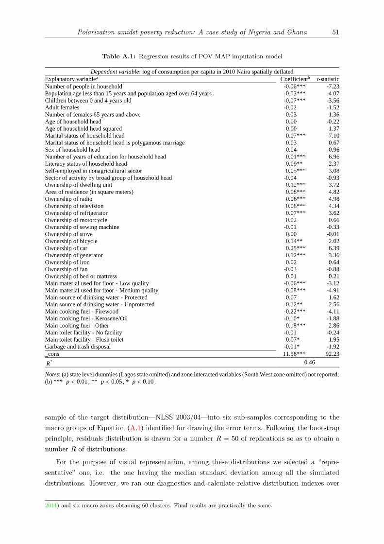
Polarization amidst poverty reduction: A case study of Nigeria and Ghana 51

Table A.1: Regression results of POV MAP imputation model

Dependent variable: log of consumption per capita in 2010 Naira spatially deflated

Explanatory variablea Coefficientb t-statistic

Number of people in household -0.06 *** -7.23

Population age less than 15 years and population aged over 64 years -0.03 *** -4.07

Children between 0 and 4 years old -0.07 *** -3.56

Adult females -0.02 -1.52

Number of females 65 years and above -0.03 -1.36

Age of household head 0.00 -0.22

Age of household head squared 0.00 -1.37

Marital status of household head 0.07 *** 7.10

Marital status of household head is polygamous marriage 0.03 0.67

Sex of household head 0.04 0.96

Number of years of education for household head 0.01 *** 6.96

Literacy status of household head 0.09 ** 2.37

Self-employed in nonagricultural sector 0.05 *** 3.08

Sector of activity by broad group of household head -0.04 -0.93

Ownership of dwelling unit 0.12 *** 3.72

Area of residence (in square meters) 0.08 *** 4.82

Ownership of radio 0.06 *** 4.98

Ownership of television 0.08 *** 4.34

Ownership of refrigerator 0.07 *** 3.62

Ownership of motorcycle 0.02 0.66

Ownership of sewing machine -0.01 -0.33

Ownership of stove 0.00 -0.01

Ownership of bicycle 0.14 ** 2.02

Ownership of car 0.25 *** 6.39

Ownership of generator 0.12 *** 3.36

Ownership of iron 0.02 0.64

Ownership of fan -0.03 -0.88

Ownership of bed or mattress 0.01 0.21

Main material used for floor - Low quality -0.06 *** -3.12

Main material used for floor - Medium quality -0.08 *** -4.91

Main source of drinking water - Protected 0.07 1.62

Main source of drinking water - Unprotected 0.12 ** 2.56

Main cooking fuel - Firewood -0.22 *** -4.11

Main cooking fuel - Kerosene/Oil -0.10 * -1.88

Main cooking fuel - Other -0.18 *** -2.86

Main toilet facility - No facility -0.01 -0.24

Main toilet facility - Flush toilet 0.07 * 1.95

Garbage and trash disposal -0.01 * -1.92

_cons 11.58 *** 92.23 2

R 0.46

Notes: (a) state level dummies (Lagos state omitted) and zone interacted variables (South West zone omitted) not reported;

(b) *** 0.01p , ** 0.05p , * 0.10p .

sample of the target distribution—NLSS 2003/04—into six sub-samples corresponding to the

macro groups of Equation (A.1) identified for drawing the error terms. Following the bootstrap

principle, residuals distribution is drawn for a number R = 50 of replications so as to obtain a

number R of distributions.

For the purpose of visual representation, among these distributions we selected a “repre-

sentative” one, i.e. the one having the median standard deviation among all the simulated

distributions. However, we ran our diagnostics and calculate relative distribution indexes over

2011) and six macro zones obtaining 60 clusters. Final results are practically the same.

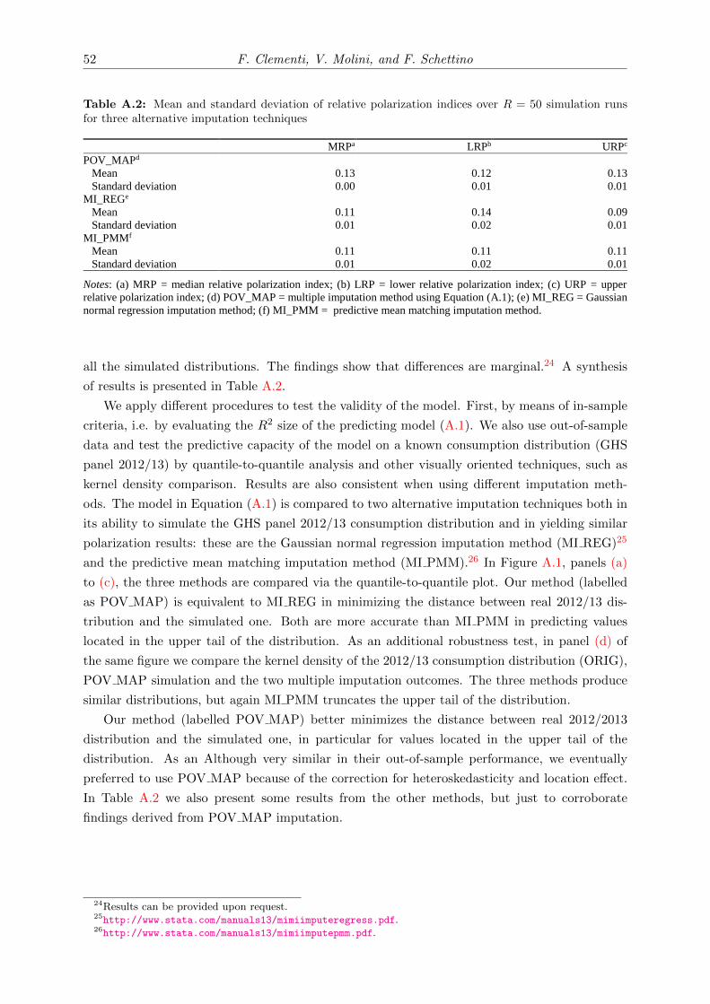
52 F. Clementi, V. Molini, and F. Schettino

Table A.2: Mean and standard deviation of relative polarization indices over R = 50 simulation runsfor three alternative imputation techniques

MRPa LRPb URPc

POV_MAPd

Mean 0.13 0.12 0.13

Standard deviation 0.00 0.01 0.01

MI_REGe

Mean 0.11 0.14 0.09

Standard deviation 0.01 0.02 0.01

MI_PMMf

Mean 0.11 0.11 0.11

Standard deviation 0.01 0.02 0.01

Notes: (a) MRP = median relative polarization index; (b) LRP = lower relative polarization index; (c) URP = upper

relative polarization index; (d) POV_MAP = multiple imputation method using Equation (A.1); (e) MI_REG = Gaussian

normal regression imputation method; (f) MI_PMM = predictive mean matching imputation method.

all the simulated distributions. The findings show that differences are marginal.24 A synthesis

of results is presented in Table A.2.

We apply different procedures to test the validity of the model. First, by means of in-sample

criteria, i.e. by evaluating the R2 size of the predicting model (A.1). We also use out-of-sample

data and test the predictive capacity of the model on a known consumption distribution (GHS

panel 2012/13) by quantile-to-quantile analysis and other visually oriented techniques, such as

kernel density comparison. Results are also consistent when using different imputation meth-

ods. The model in Equation (A.1) is compared to two alternative imputation techniques both in

its ability to simulate the GHS panel 2012/13 consumption distribution and in yielding similar

polarization results: these are the Gaussian normal regression imputation method (MI REG)25

and the predictive mean matching imputation method (MI PMM).26 In Figure A.1, panels (a)

to (c), the three methods are compared via the quantile-to-quantile plot. Our method (labelled

as POV MAP) is equivalent to MI REG in minimizing the distance between real 2012/13 dis-

tribution and the simulated one. Both are more accurate than MI PMM in predicting values

located in the upper tail of the distribution. As an additional robustness test, in panel (d) of

the same figure we compare the kernel density of the 2012/13 consumption distribution (ORIG),

POV MAP simulation and the two multiple imputation outcomes. The three methods produce

similar distributions, but again MI PMM truncates the upper tail of the distribution.

Our method (labelled POV MAP) better minimizes the distance between real 2012/2013

distribution and the simulated one, in particular for values located in the upper tail of the

distribution. As an Although very similar in their out-of-sample performance, we eventually

preferred to use POV MAP because of the correction for heteroskedasticity and location effect.

In Table A.2 we also present some results from the other methods, but just to corroborate

findings derived from POV MAP imputation.

24Results can be provided upon request.25http://www.stata.com/manuals13/mimiimputeregress.pdf.26http://www.stata.com/manuals13/mimiimputepmm.pdf.

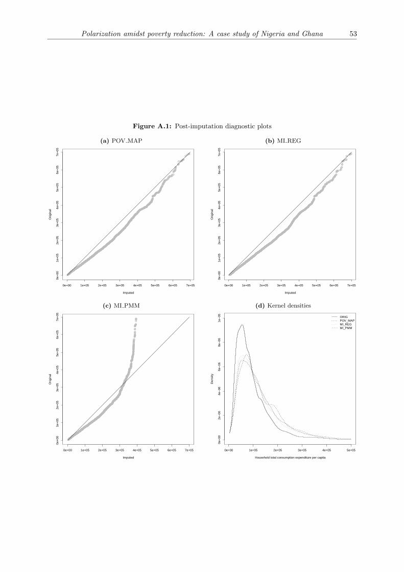
Polarization amidst poverty reduction: A case study of Nigeria and Ghana 53

Figure A.1: Post-imputation diagnostic plots

(a) POV MAP

●●●●●●●●●●●●●●●●●●●●●●●●●●●●●●●●●●●●●●●●●●●●●●●●●●●●●●●●●●●●●●●●●●●●●●●●●●●●●●●●●●●●●●●●●●●●●●●●●●●●●●●●●●●●●●●●●●●●●●●●●●●●●●●●●●●●●●●●●●●●●●●●●●●●●●●●●●●●●●●●●●●●●●●●●●●●●●●●●●●●●●●●●●●●●●●●●●●●●●●●●●●●

●●●●●●●●●●●●●●●●●●●●●●●●●●●●●●●●●●●●●●●●●●●●●●●●●●●●●●●●●●●●●●●●●●●●●●●●●●●●●●●●●●●●●●●●●●●●●●●●●●●●●●●●●●●●●●●●●●●●●●●●●●●●●●●●●●●●●●●●●●●●●●●●●●●●●●●●●●●●●●●●●●●●●●●●●●●●●●●●●●●●●●●●●●●●●●●●●●●●●●●●●●●●●●●●●●●●●●●●●●●●●●●●●●●●●●●●●●●●●●●●●●●●●●●●●●●●●●●●●●●●●●●●●●●●●●●●●●●●●●●●●●●●●●●●●●●●●●●●●●●●●●●●●●●●●●●●●●●●●●●●●●●●●●●●●●●●●●●●●●●●●●●●●●●●●●●●●●●●●●●●●●●●●●●●●●●●●●●●●●●●●●●●●●●●●●●●●●●●●●●●●●●●●●●●●●●●●●●●●●●●●●●●●●●●●●●●●●●●●●●●●●●●●●●●●●●●●●●●●●●●●●●●●●●●●●●●●●●●●●●●●●●●●●●●●●●●●●●●●●●●●●●●●●●●●●●●●●●●●●●●●●●●●●●●●●●●●●●●●●●●●●

●●●●●●●●●●●●●●●●●●●●●●●●●●●●●●●●●●●●●●●●●●●●●●●●●●●●●●●●●●●●●●●●●●●●●●●●●●●●●●●●●●●●●●●●●●●●●●●●●●●●●●●●●●●●●●●●●●●●●●●●●●●●●●●●●●●●●●●●●●●●●●●●●●●●●●●●●●●●●●●●●●●●●●●●●●●●●●●●●●●●●●●●●●●●●●●●●●●●●●●●●●●●●●●●●●●●●●●●●●●●●●●●●●●●●●●●●●●●●●●●●●●●●●●●●●●●●●●●●●●●●●●●●●●●●●●●●●●●●●●●●●●●●●●●●●●●●●●●●●●●●●●●●●●●●●●●●●●●●●●●●●●●●●●●●●●●●●●●●●●●●●●●●●●●●●●●●●●●●●●●●●●●●●●●●●●●●●●●●●●●●●●●●●●●●●●●●●●●●●●●●●●●●●●●●●●●●●●●●●●●●●●●●●●●●●●●●●●●●●●●●●●●●●●●●●●●●●●●●●●●●●●●●●●●●●●●●●●●●●●●●●●●●●●●●●●●●●●●●●●●●●●●●●●●●●●●●●●●●●●●●●●●●●●●●●●●●●●●●●●●●●●●●●●●●●●●●●●●●●●●●●●●●●●●●●●●●●●●●●●●●●●●●●●●●●●●●●●●●●●●●●●●●●●●●●●●●●●●●●●●●●●●●●●●●●●●●●●●●●●●●●●●●●●●●●●●●●●●●●●●●●●●●●●●●●●●●●●●●●●●●●●●●●●●●●●●●●●●●●●●●●●●●●●●●●●●●●●●●●●●●●●●●●●●

●●●●●●●●●●●●●●●●●●●●●●●●●●●●●●●●●●●●●●●●●●●●●●●●●●●●●●●●●●●●●●●●●●●●●●●●●●●●●●●●●●●●●●●●●●●●●●●●●●●●●●●●●●●●●●●●●●●●●●●●●●●●●●●●●●●●●●●●●●●●●●●●●●●●●●●●●●●●●●●●●●●●●●●●●●●●●●●●●●●●●●●●●●●●●●●●●●●●●●●●●●●●●●●●●●●●●●●●●●●●●●●●●●●●●●●●●●●●●●●●●●●●●●●●●●●●●●●●●●●●●●●●●●●●●●●●●●●●●●●●●●●●●●●●●●●●●●●●●●●●●●●●●●●●●●●●●●●●●●●●●●●●●●●●●●●●●●●●●●●●●●●●●●●●●●●●●●●●●●●●●●●●●●●●●●●●●●●●●●●●●●●●●●●●●●●●●●●●●●●●●●●●●●●●●●●●●●●●●●●●●●●●●●●●●●●●●●●●●●●●●●●●●●●●●●●●●●●●●●●●●●●●●●●●●●●●●●●●●●●●●●●●●●●●●●●●●●●●●●●●●●●●●●●●●●●●●●●●●●●●●●●●●●●●●●●●●●●●●●●●●●●●●●●●●●●●●●●●●●●●●●●●●●●●●●●●●●●●●●●●●●●●●●●●●●●●●●●●●●●●●●●●●●●●●●●●●●●●●●●●●●●●●●●●●●●●●●●●●●●●●●●●●●●●●●●●●●●●●●●●●●●●●●●●●●●●●●●●●●●●●●●●●●●●●●●●●●●●●●●●●●●●●●●●●●●●●●●●●●●●●●●●●●●●●●●●●●●●●●●●●●●●●●●●●●●●●●●●●●●●●●●●●●●●●●●●●●●●●●●●●●●●●●●●●●●●●●●●●●●●●●●●●●●●●●●●●●●●●●●●●●●●●●●●●●●●●●●●●●●●●●●●●●●●●●●●●●●●

●●●●●●●●●●●●●●●●●●●●●●●●●●●●●●●●●●●●●●●●●●●●●●●●●●●●●●●●●●●●●●●●●●●●●●●●●●●●●●●●●●●●●●●●●●●●●●●●●●●●●●●●●●●●●●●●●●●●●●●●●●●●●●●●●●●●●●●●●●●●●●●●●●●●●●●●●●●●●●●●●●●●●●●●●●●●●●●●●●●●●●●●●●●●●●●●●●●●●●●●●●●●●●●●●●●●●●●●●●●●●●●●●●●●●●●●●●●●●●●●●●●●●●●●●●●●●●●●●●●●●●●●●●●●●●●●●●●●●●●●●●●●●●●●●●●●●●●●●●●●●●●●●●●●●●●●●●●●●●●●●●●●●●●●●●●●●●●●●●●●●●●●●●●●●●●●●●●●●●●●●●●●●●●●●●●●●●●●●●●●●●●●●●●●●●●●●●●●●●●●●●●●●●●●●●●●●●●●●●●●●●●●●●●●●●●●●●●●●●●●●●●●●●●●●●●●●●●●●●●●●●●●●●●●●●●●●●●●●●●●●●●●●●●●●●●●●●●●●●●●●●●●●●●●●●●●●●●●●●●●●●●●●●●●●●●●●●●●●●●●●●●●●●●●●●●●●●●●●●●●●●●●●●●●●●●●●●●●●●●●●●●●●●●●●●●●●●●●●●●●●●●●●●●●●●●●●●●●●●●●●●●●●●●●●●●●●●●●●●●●●●●●●●●●●●●●●●●●●●●●●●●●●●●●●●●●●●●●●●●●●●●●●●●●●●●●●●●●●●●●●●●●●●●●●●●●●●●●●●●●●●●●●●●●●●●●●●●●●●●●●●●●●●●●●●●●●●●●●●●●●●●●●●●●●●●●●●●●●●●●●●●●●●●●●●●●●●●●●●●●●●●●●●●●●●●●●●

●●●●●●●●●●●●●●●●●●●●●●●●●●●●●●●●●●●●●●●●●●●●●●●●●●●●●●●●●●●●●●●●●●●●●●●●●●●●●●●●●●●●●●●●●●●●●●●●●●●●●●●●●●●●●●●●●●●●●●●●●●●●●●●●●●●●●●●●●●●●●●●●●●●●●●●●●●●●●●●●●●●●●●●●●●●●●●●●●●●●●●●●●●●●●●●●●●●●●●●●●●●●●●●●●●●●●●●●●●●●●●●●●●●●●●●●●●●●●●●●●●●●●●●●●●●●●●●●●●●●●●●●●●●●●●●●●●●●●●●●●●●●●●●●●●●●●●●●●●●●●●●●●●●●●●●●●●●●●●●●●●●●●●●●●●●●●●●●●●●●●●●●●●●●●●●●●●●●●●●●●●●●●●●●●●●●●●●●●●●●●●●●●●●●●●●●●●●●●●●●●●●●●●●●●●●●●●●●●●●●●●●●●●●●●●●●●●●●●●●●●●●●●●●●●●●●●●●●●●●●●●●●●●●●●●●●●●●●●●●●●●●●●●●●●●●●●●●●●●●●●●●●●●●●●●●●●●●●●●●●●●●●●●●●●●●●●●●●●●●●●●●●●●●●●●●●●●●●●●●●●●●●●●●●●●●●●●●●●●●●●●●●●●●●●●●●●●●●●●●●●●●●●●●●●●●●●●●●●●●●●●●●●●●●●●●●●●●●●●●●●●●●●●●●●●●●●●●●●●●●●●●●●●●●●●●●●●●●●●●●●●●●●●●●●●●●●●●●●●●●●●●●●●●●●●●●●●●●●●●●●●●●●●●●●●●●●●●●●●●

●●●●●●●●●●●●●●●●●●●●●●●●●●●●●●●●●●●●●●●●●●●●●●●●●●●●●●●●●●●●●●●●●●●●●●●●●●●●●●●●●●●●●●●●●●●●●●●●●●●●●●●●●●●●●●●●●●●●●●●●●●●●●●●●●●●●●●●●●●●●●●●●●●●●●●●●●●●●●●●●●●●●●●●●●●●●●●●●●●●●●●●●●●●●●●●●●●●●●●●●●●●●●●●●●●●●●●●●●●●●●●●●●●●●●●●●●●●●●●●●●●●●●●●●●●●●●●●●●●●●●●●●●●●●●●●●●●●●●●●●●●●●●●●●●●●●●●●●●●●●●●●●●●●●●●●●●●●●●●●●●●●●●●●●●●●●●●●●●●●●●●●●●●●●●●●●●●●●●●●●●●●●●●●●●●●●●●●●●●●●●●●●●●●●●●●●●●●●●●●●●●●●●●●●●●●●●●●●●●●●●●●●●●●●●●●●●●●●●●●●●●●●●●●●●●●●●●●●●●●●●●●●●●●●●●●●●●●●●●●●●●●●●●●●●●●●●●●●●●●●●●●●●●●●●●●●●●●●●●●●●●●●●●●●●●●●●●●●●●●●●●●●●●●●●●●●●●●●●●●●●●●●●●●●●●●●●●●●●●●●●●●●●●●●●●●●●●●●●●●●●●●●●●●●●●●●●●●●●●●●●●●●●●●●●●●●●●●●●●●●●●●●●●●●●●●●●●●●●●●●●●●●●●●●●●●●●●●●●●●●●●●●●●

●●●●●●●●●●●●●●●●●●●●●●●●●●●●●●●●●●●●●●●●●●●●●●●●●●●●●●●●●●●●●●●●●●●●●●●●●●●●●●●●●●●●●●●●●●●●●●●●●●●●●●●●●●●●●●●●●●●●●●●●●●●●●●●●●●●●●●●●●●●●●●●●●●●●●●●●●●●●●●●●●●●●●●●●●●●●●●●●●●●●●●●●●●●●●●●●●●●●●●●●●●●●●●●●●●●●●●●●●●●●●●●●●●●●●●●●●●●●●●●●●●●●●●●●●●●●●●●●●●●●●●●●●●●●●●●●●●●●●●●●●●●●●●●●●●●●●●●●●●●●●●●●●●●●●●●●●●●●●●●●●●●●●●●●●●●●●●●●●●●●●●●●●●●●●●●●●●●●●●●●●●●●●●●●●●●●●●●●●●●●●●●●●●●●●●●●●●●●●●●●●●●●●●●●●●●●●●●●●●●●●●●●●●●●●●●●●●●●●●●●●●●●●●●●●●●●●●●●●●●●●●●●●●●●●●●●●●●●●●●●●●●●●●●●●●●●●●●●●●●●●●●●●●●●●●●●●●●●●●●●●●●●●●●●●●●●●●●●●●●●●●●●●●●●●●●●●●●●●●●●●●●●●●●●●●●●●●●●●●●●●●●●●●●●●●●●●●●●●●●●●●●●

●●●●●●●●●●●●●●●●●●●●●●●●●●●●●●●●●●●●●●●●●●●●●●●●●●●●●●●●●●●●●●●●●●●●●●●●●●●●●●●●●●●●●●●●●●●●●●●●●●●●●●●●●●●●●●●●●●●●●●●●●●●●●●●●●●●●●●●●●●●●●●●●●●●●●●●●●●●●●●●●●●●●●●●●●●●●●●●●●●●●●●●●●●●●●●●●●●●●●●●●●●●●●●●●●●●●●●●●●●●●●●●●●●●●●●●●●●●●●●●●●●●●●●●●●●●●●●●●●●●●●●●●●●●●●●●●●●●●●●●●●●●●●●●●●●●●●●●●●●●●●●●●●●●●●●●●●●●●●●●●●●●●●●●●●●●●●●●●●●●●●●●●●●●●●●●●●●●●●●●●●●●●●●●●●●●●●●●●●●●●●●●●●●●●●●●●●●●●●●●●●●●●●●●●●●●●●●●●●●●●●●●●●●●●●●●●●●●●●●●●●●●●●●●●●●●●●●●●●●●●●●●●●●●●●●●●●●●●●●●●●●●●●●●●●●●●●●●●●●●●●●●●●●●●●●●●●●●●●

●●●●●●●●●●●●●●●●●●●●●●●●●●●●●●●●●●●●●●●●●●●●●●●●●●●●●●●●●●●●●●●●●●●●●●●●●●●●●●●●●●●●●●●●●●●●●●●●●●●●●●●●●●●●●●●●●●●●●●●●●●●●●●●●●●●●●●●●●●●●●●●●●●●●●●●●●●●●●●●●●●●●●●●●●●●●●●●●●●●●●●●●●●●●●●●●●●●●●●●●●●●●●●●●●●●●●●●●●●●●●●●●●●●●●●●●●●●●●●●●●●●●●●●●●●●●●●●●●●●●●●●●●●●●●●●●●●●●●●●●●●●●●●●●●●●●●●●●●●●●●●●●●●●●●●●●●●●●●●●●●●●●●●●●●●●●●●●●●●●●●●●●●●●●●●●●●●●●●●●●●●●●●●●●●●●●●●●●●●●●●●●●●●●●●●●●●●●●●●●●●●●●●●●●●●●●●●●●●●●●●●●●●●●●●●●●●●●●●●●●●●●●●●●●●●●●●●●●●●●●●●●●●●●●

●●●●●●●●●●●●●●●●●●●●●●●●●●●●●●●●●●●●●●●●●●●●●●●●●●●●●●●●●●●●●●●●●●●●●●●●●●●●●●●●●●●●●●●●●●●●●●●●●●●●●●●●●●●●●●●●●●●●●●●●●●●●●●●●●●●●●●●●●●●●●●●●●●●●●●●●●●●●●●●●●●●●●●●●●●●●●●●●●●●●●●●●●●●●●●●●●●●●●●●●●●●●●●●●●●●●●●●●●●●●●●●●●●●●●●●●●●●●●●●●●●●●●●●●●●●●●●●●●●●●●●●●●●●●●●●●●●●●●●●●●●●●●●●●●●●●●●●●●●●●●●●●●●●●●●●●●●●●●●●●●●●●●●●●●●●●●●●●●●●●●●●●●●●●●

●●●●●●●●●●●●●●●●●●●●●●●●●●●●●●●●●●●●●●●●●●●●●●●●●●●●●●●●●●●●●●●●●●●●●●●●●●●●●●●●●●●●●●●●●●●●●●●●●●●●●●●●●●●●●●●●●●●●●●●●●●●●●●●●●●●●●●●●●●●●●●●●●●●●●●●●●●●●●●●●●●●●●●●●●●●●●●●●●●●●●●●●●●●●●●●●●●●●●●●●●●●●●●●●●●●●●●●●●●●●●●●●●●●●●●●●●●●●●●●●●●●●●●●●●●●●●●●●●●●●●●●●●●●●●●●●●●●●●●●●●●●●●●●●●●●●●●●●●●●●●●●●●●●●●●●●●●●●●●●●●●●●●●●●●●●●●●●●●●●●●●●●●●●●●●●●●●●●●

●●●●●●●●●●●●●●●●●●●●●●●●●●●●●●●●●●●●●●●●●●●●●●●●●●●●●●●●●●●●●●●●●●●●●●●●●●●●●●●●●●●●●●●●●●●●●●●●●●●●●●●●●●●●●●●●●●●●●●●●●●●●●●●●●●●●●●●●●●●●●●●●●●●●●●●●●●●●●●●●●●●●●●●●●●●●●●●●●●●●●●●●●●●●●●●●●●●●●●●●●●●●●●●●●●●●●●●●●●●●●●●●●●●●●●●●●●●●●●●●●●●●●●●●●●●●●●●●●●●●●●●●●●●●●●●●●●●●●●●●●●●●●●●●●●●●●●●●●●●●●●●●●●●●●●●●●

●●●●●●●●●●●●●●●●●●●●●●●●●●●●●●●●●●●●●●●●●●●●●●●●●●●●●●●●●●●●●●●●●●●●●●●●●●●●●●●●●●●●●●●●●●●●●●●●●●●●●●●●●●●●●●●●●●●●●●●●●●●●●●●●●●●●●●●●●●●●●●●●●●●●●●●●●●●●●●●●●●●●●●●●●●●●●●●●●●●●●●●●●●●●●●●●●●●●●●●●●●●●●●●●●●●●●●●●●●●●●●●●●●●●●●●●●●●●●●●●●

●●●●●●●●●●●●●●●●●●●●●●●●●●●●●●●●●●●●●●●●●●●●●●●●●●●●●●●●●●●●●●●●●●●●●●●●●●●●●●●●●●●●●●●●●●●●●●●●●●●●●●●●●●●●●●●●●●●●●●●●●●●●●●●●●●●●●●●●●●●●●●●●●●●●●●●●●●●●●●●●●●●●●●●●●●●●●●●●●●●●●●●●●●●●●●●●●●●●●●●●●●●●●●●●●●●●

●●●●●●●●●●●●●●●●●●●●●●●●●●●●●●●●●●●●●●●●●●●●●●●●●●●●●●●●●●●●●●●●●●●●●●●●●●●●●●●●●●●●●●●●●●●●●●●●●●●●●●●●●●●●●●●●●●●●●●●●●●●●●●●●●●●●●●●●●●●●●●●●●●●●●●●●●●●●●●●●●●●●●●●●●●●●●●●●●●●●●●●●●●●●●●●●●●●●●●●●●●●●●●●●●●●●●●●●●●●●●●●●●●●●●●●●●●●●●●●●●●●●●●●●●●●●●●●●●●●●●●●●●●●●●●●●●●●●●●●●●●●●●●●●●●●●●●●●●●●●●●●●●●●●●●●●●●●●●●●●●●●●●●●●●●●●●●●●●●●●●●●

●●●●●●●●●●●●●●●●●●●●●●●●●●●●●●●●●●●●●●●●●●●●●●●●●●●●●●●●●●●●●●●●●●●●●●●●●●●●●●●●●●●●●●●●●●●●●●●●●●●●●●●●●●●●●●●●●●●●●●●●●●●●●●●●●●●●

●●●●●●●●●●●●●●●●●●●●●●●●●●●●●●●●●●●●●●●●●●●●●●●●●●●●●●●●●●●●●●●●●●●●●●●●●●●●●●●●●●●●●●●●●●●●●●●●●●●●●●●●●●●●●●●●●●●●●●●●●●●●●●●●●●●●●●●●●●●●●●●●●●●●●●●●●●●●●●●●●●●●●●●●●●●●●●●●●●●●●●●●●●●●●●●●●●●●●●●●●●●●●●●●●●●●●●●●●●●●●●●●●●●●●●●●●●●●●●●●●●●●●●●●●●●●●●●●●●●●●●●●●●●●●●●●●●●●●●●●●●●●●

●●●●●●●●●●●●●●●●●●●●●●●●●●●●●●●●●●●●●●●●●●●●●●●●●●●●●●●●●●●●●●●●●●●●●●●●●●●●●●●●●●●●●●●●●●●●●●●●●●●●●●●●●●●●●●●●●●●●●●●●●●●●●●●●●●●●●●●●●●

●●●●●●●●●●●●●●●●●●●●●●●●●●●●●●●●●●●●●●●●●●●●●●●●●●●●●●●●●●●●●●●●●●●●●●●●●●●●●●●●●●●●●●●●●●●

●●●●●●●●●●●●●●●●●●●●●●●●●●●●●●●●●●●●●●●●●●●●●●●●●●●●●●●●●●●●●●●●●●●●●●●●●●●●●●●●●●●●●●●●●●●●

●●●●●●●●●●●●●●●●●●●●●●●●●●●●●●●●●●●●●●●●●●●●●●●●●●●●●●●●●●●●●●●●●●●●●●●●●●●●●●●●●●●●●●●●●●●●●●●●●●●●●●●●●●●

●●●●●●●●●●●●●●●●●●●●●●●●●●●●●●●●●●●●●●●●●●●●●●●●●●●●●●●●●●

●●●●●●●●●●●●●●●●●●●●●●●●●●●●●●●●●●●●●●●●●●●●●●●●●●●●●●●

●●●●●●●●●●●●●●●●●●●●●●

●●●●●●●●●●●●●●●●●●●●●●●●●●●●●

●●●●●●●●●●●●●●●

●●●●●●●●●●●●●●●●●●●●●●●●●●●●●

●●●●●●●●●●●●●●●●●●

●●●●●●●●●●●●●●●●●●●●●●●●●●●●●●●●●●●●●

●●●●●

●●●●●

●●●●●●●●●

●●

● ●●●●●●

●●●●

0e+00 1e+05 2e+05 3e+05 4e+05 5e+05 6e+05 7e+05

0e+

001e

+05

2e+

053e

+05

4e+

055e

+05

6e+

057e

+05

Imputed

Orig

inal

(b) MI REG

●●●●●●●●●●●●●●●●●●●●●●●●●●●●●●●●●●●●●●●●●●●●●●●●●●●●●●●●●●●●●●●●●●●●●●●●●●●●●●●●

●●●●●●●●●●●●●●●●●●●●●●●●●●●●●●●●●●●●●●●●●●●●●●●●●●●●●●●●●●●●●●●●●●●●●●●●●●●●●●●●●●●●●●●●●●●●●●●●●●●●●●●●●●●●●●●●●●●●●●●●●●●●●●●●●●●●●●●●●●●●●●●●●●●●●●●●●●●●●●●●●●●●●●●●●●●●●●●●●●●●●●●●●●●●●●●●●●●●●●●●●●●●●●●●●●●●●●●●●●●●●●●●●●●●●●●●●●●●●●●●●●●●●●●●●●●●●●●●●●●●●●●●●●●●●●●●●●●●●●●●●●●●●●●●●●●●●●●●●●●●●●●●●●●●●●●●●●●●●●●●●●●●●●●●●●●●●●●●●●●●●●●●●●●●●●●●●●●●●●●●●●

●●●●●●●●●●●●●●●●●●●●●●●●●●●●●●●●●●●●●●●●●●●●●●●●●●●●●●●●●●●●●●●●●●●●●●●●●●●●●●●●●●●●●●●●●●●●●●●●●●●●●●●●●●●●●●●●●●●●●●●●●●●●●●●●●●●●●●●●●●●●●●●●●●●●●●●●●●●●●●●●●●●●●●●●●●●●●●●●●●●●●●●●●●●●●●●●●●●●●●●●●●●●●●●●●●●●●●●●●●●●●●●●●●●●●●●●●●●●●●●●●●●●●●●●●●●●●●●●●●●●●●●●●●●●●●●●●●●●●●●●●●●●●●●●●●●●●●●●●●●●●●●●●●●●●●●●●●●●●●●●●●●●●●●●●●●●●●●●●●●●●●●●●●●●●●●●●●●●●●●●●●●●●●●●●●●●●●●●●●●●●●●●●●●●●●●●●●●●●●●●●●●●●●●●●●●●●●●●●●●●●●●●●●●●●●●●●●●●●●●●●●●●●●●●●●●●●●●●●●●●●●●●●●●●●●●●●●●●●●●●●●●●●●●●●●●●●●●●●●●●●●●●●●●●●●●●●●●●●●●●●●●●●●●●●●●●●●●●●●●●●●●●●●●●●●●●●●●●●●●●●●●●●●●●●●●●●●●●●●●●●●●●●●●●●●●●●●●●●●●●●●●●●●●●●●●●●●●●●●●●●●●●●●●●●●●●●●●●●●●●●●●●●●●●●●

●●●●●●●●●●●●●●●●●●●●●●●●●●●●●●●●●●●●●●●●●●●●●●●●●●●●●●●●●●●●●●●●●●●●●●●●●●●●●●●●●●●●●●●●●●●●●●●●●●●●●●●●●●●●●●●●●●●●●●●●●●●●●●●●●●●●●●●●●●●●●●●●●●●●●●●●●●●●●●●●●●●●●●●●●●●●●●●●●●●●●●●●●●●●●●●●●●●●●●●●●●●●●●●●●●●●●●●●●●●●●●●●●●●●●●●●●●●●●●●●●●●●●●●●●●●●●●●●●●●●●●●●●●●●●●●●●●●●●●●●●●●●●●●●●●●●●●●●●●●●●●●●●●●●●●●●●●●●●●●●●●●●●●●●●●●●●●●●●●●●●●●●●●●●●●●●●●●●●●●●●●●●●●●●●●●●●●●●●●●●●●●●●●●●●●●●●●●●●●●●●●●●●●●●●●●●●●●●●●●●●●●●●●●●●●●●●●●●●●●●●●●●●●●●●●●●●●●●●●●●●●●●●●●●●●●●●●●●●●●●●●●●●●●●●●●●●●●●●●●●●●●●●●●●●●●●●●●●●●●●●●●●●●●●●●●●●●●●●●●●●●●●●●●●●●●●●●●●●●●●●●●●●●●●●●●●●●●●●●●●●●●●●●●●●●●●●●●●●●●●●●●●●●●●●●●●●●●●●●●●●●●●●●●●●●●●●●●●●●●●●●●●●●●●●●●●●●●●●●●●●●●●●●●●●●●●●●●●●●●●●●●●●●●●●●●●●●●●●●●●●●●●●●●●●●●●●●●●●●●●●●●●●●●●●●●●●●●●●●●●●●●●●●●●●●●●●●●●●●●●●●●●●●●●●●●●●●●●●●●●●●●●●●●●●●●●●●●●●●●●●●●●●●●●●●●●●●●●●●●●

●●●●●●●●●●●●●●●●●●●●●●●●●●●●●●●●●●●●●●●●●●●●●●●●●●●●●●●●●●●●●●●●●●●●●●●●●●●●●●●●●●●●●●●●●●●●●●●●●●●●●●●●●●●●●●●●●●●●●●●●●●●●●●●●●●●●●●●●●●●●●●●●●●●●●●●●●●●●●●●●●●●●●●●●●●●●●●●●●●●●●●●●●●●●●●●●●●●●●●●●●●●●●●●●●●●●●●●●●●●●●●●●●●●●●●●●●●●●●●●●●●●●●●●●●●●●●●●●●●●●●●●●●●●●●●●●●●●●●●●●●●●●●●●●●●●●●●●●●●●●●●●●●●●●●●●●●●●●●●●●●●●●●●●●●●●●●●●●●●●●●●●●●●●●●●●●●●●●●●●●●●●●●●●●●●●●●●●●●●●●●●●●●●●●●●●●●●●●●●●●●●●●●●●●●●●●●●●●●●●●●●●●●●●●●●●●●●●●●●●●●●●●●●●●●●●●●●●●●●●●●●●●●●●●●●●●●●●●●●●●●●●●●●●●●●●●●●●●●●●●●●●●●●●●●●●●●●●●●●●●●●●●●●●●●●●●●●●●●●●●●●●●●●●●●●●●●●●●●●●●●●●●●●●●●●●●●●●●●●●●●●●●●●●●●●●●●●●●●●●●●●●●●●●●●●●●●●●●●●●●●●●●●●●●●●●●●●●●●●●●●●●●●●●●●●●●●●●●●●●●●●●●●●●●●●●●●●●●●●●●●●●●●●●●●●●●●●●●●●●●●●●●●●●●●●●●●●●●●●●●●●●●●●●●●●●●●●●●●●●●●●●●●●●●●●●●●●●●●●●●●●●●●●●●●●●●●●●●●●●●●●●●●●●●●●●●●●●●●●●●●●●●●●●●●●●●●●●●●●●●●●●●●●●●●●●●●●●

●●●●●●●●●●●●●●●●●●●●●●●●●●●●●●●●●●●●●●●●●●●●●●●●●●●●●●●●●●●●●●●●●●●●●●●●●●●●●●●●●●●●●●●●●●●●●●●●●●●●●●●●●●●●●●●●●●●●●●●●●●●●●●●●●●●●●●●●●●●●●●●●●●●●●●●●●●●●●●●●●●●●●●●●●●●●●●●●●●●●●●●●●●●●●●●●●●●●●●●●●●●●●●●●●●●●●●●●●●●●●●●●●●●●●●●●●●●●●●●●●●●●●●●●●●●●●●●●●●●●●●●●●●●●●●●●●●●●●●●●●●●●●●●●●●●●●●●●●●●●●●●●●●●●●●●●●●●●●●●●●●●●●●●●●●●●●●●●●●●●●●●●●●●●●●●●●●●●●●●●●●●●●●●●●●●●●●●●●●●●●●●●●●●●●●●●●●●●●●●●●●●●●●●●●●●●●●●●●●●●●●●●●●●●●●●●●●●●●●●●●●●●●●●●●●●●●●●●●●●●●●●●●●●●●●●●●●●●●●●●●●●●●●●●●●●●●●●●●●●●●●●●●●●●●●●●●●●●●●●●●●●●●●●●●●●●●●●●●●●●●●●●●●●●●●●●●●●●●●●●●●●●●●●●●●●●●●●●●●●●●●●●●●●●●●●●●●●●●●●●●●●●●●●●●●●●●●●●●●●●●●●●●●●●●●●●●●●●●●●●●●●●●●●●●●●●●●●●●●●●●●●●●●●●●●●●●●●●●●●●●●●●●●●●●●●●●●●●●●●●●●●●●●●●●●●●●●●●●●●●●●●●●●●●●●●●●●●●●●●●●●●●●●●●●●●●●●●●●●●●●●●●●

●●●●●●●●●●●●●●●●●●●●●●●●●●●●●●●●●●●●●●●●●●●●●●●●●●●●●●●●●●●●●●●●●●●●●●●●●●●●●●●●●●●●●●●●●●●●●●●●●●●●●●●●●●●●●●●●●●●●●●●●●●●●●●●●●●●●●●●●●●●●●●●●●●●●●●●●●●●●●●●●●●●●●●●●●●●●●●●●●●●●●●●●●●●●●●●●●●●●●●●●●●●●●●●●●●●●●●●●●●●●●●●●●●●●●●●●●●●●●●●●●●●●●●●●●●●●●●●●●●●●●●●●●●●●●●●●●●●●●●●●●●●●●●●●●●●●●●●●●●●●●●●●●●●●●●●●●●●●●●●●●●●●●●●●●●●●●●●●●●●●●●●●●●●●●●●●●●●●●●●●●●●●●●●●●●●●●●●●●●●●●●●●●●●●●●●●●●●●●●●●●●●●●●●●●●●●●●●●●●●●●●●●●●●●●●●●●●●●●●●●●●●●●●●●●●●●●●●●●●●●●●●●●●●●●●●●●●●●●●●●●●●●●●●●●●●●●●●●●●●●●●●●●●●●●●●●●●●●●●●●●●●●●●●●●●●●●●●●●●●●●●●●●●●●●●●●●●●●●●●●●●●●●●●●●●●●●●●●●●●●●●●●●●●●●●●●●●●●●●●●●●●●●●●●●●●●●●●●●●●●●●●●●●●●●●●●●●●●●●●●●●●●●●●●●●●●●●●●●●●●●●●●●●●●●●●●●●●●●●●●●●●●●●●●●●●●●●●●●●●●●●●●●●●●

●●●●●●●●●●●●●●●●●●●●●●●●●●●●●●●●●●●●●●●●●●●●●●●●●●●●●●●●●●●●●●●●●●●●●●●●●●●●●●●●●●●●●●●●●●●●●●●●●●●●●●●●●●●●●●●●●●●●●●●●●●●●●●●●●●●●●●●●●●●●●●●●●●●●●●●●●●●●●●●●●●●●●●●●●●●●●●●●●●●●●●●●●●●●●●●●●●●●●●●●●●●●●●●●●●●●●●●●●●●●●●●●●●●●●●●●●●●●●●●●●●●●●●●●●●●●●●●●●●●●●●●●●●●●●●●●●●●●●●●●●●●●●●●●●●●●●●●●●●●●●●●●●●●●●●●●●●●●●●●●●●●●●●●●●●●●●●●●●●●●●●●●●●●●●●●●●●●●●●●●●●●●●●●●●●●●●●●●●●●●●●●●●●●●●●●●●●●●●●●●●●●●●●●●●●●●●●●●●●●●●●●●●●●●●●●●●●●●●●●●●●●●●●●●●●●●●●●●●●●●●●●●●●●●●●●●●●●●●●●●●●●●●●●●●●●●●●●●●●●●●●●●●●●●●●●●●●●●●●●●●●●●●●●●●●●●●●●●●●●●●●●●●●●●●●●●●●●●●●●●●●●●●●●●●●●●●●●●●●●●●●●●●●●●●●●●●●●●●●●●●●●●●●●●●●●●●●●●●●●●●●●●●●●●●●●●●●●●●●●●●●●●●●●●●●●●●●●●●●●●●

●●●●●●●●●●●●●●●●●●●●●●●●●●●●●●●●●●●●●●●●●●●●●●●●●●●●●●●●●●●●●●●●●●●●●●●●●●●●●●●●●●●●●●●●●●●●●●●●●●●●●●●●●●●●●●●●●●●●●●●●●●●●●●●●●●●●●●●●●●●●●●●●●●●●●●●●●●●●●●●●●●●●●●●●●●●●●●●●●●●●●●●●●●●●●●●●●●●●●●●●●●●●●●●●●●●●●●●●●●●●●●●●●●●●●●●●●●●●●●●●●●●●●●●●●●●●●●●●●●●●●●●●●●●●●●●●●●●●●●●●●●●●●●●●●●●●●●●●●●●●●●●●●●●●●●●●●●●●●●●●●●●●●●●●●●●●●●●●●●●●●●●●●●●●●●●●●●●●●●●●●●●●●●●●●●●●●●●●●●●●●●●●●●●●●●●●●●●●●●●●●●●●●●●●●●●●●●●●●●●●●●●●●●●●●●●●●●●●●●●●●●●●●●●●●●●●●●●●●●●●●●●●●●●●●●●●●●●●●●●●●●●●●●●●●●●●●●●●●●●●●●●●●●●●●●●●●●●●●●●●●●●●●●●●●●●●●●●●●●●●●●●●●●●●●●●●●●●●●

●●●●●●●●●●●●●●●●●●●●●●●●●●●●●●●●●●●●●●●●●●●●●●●●●●●●●●●●●●●●●●●●●●●●●●●●●●●●●●●●●●●●●●●●●●●●●●●●●●●●●●●●●●●●●●●●●●●●●●●●●●●●●●●●●●●●●●●●●●●●●●●●●●●●●●●●●●●●●●●●●●●●●●●●●●●●●●●●●●●●●●●●●●●●●●●●●●●●●●●●●●●●●●●●●●●●●●●●●●●●●●●●●●●●●●●●●●●●●●●●●●●●●●●●●●●●●●●●●●●●●●●●●●●●●●●●●●●●●●●●●●●●●●●●●●●●●●●●●●●●●●●●●●●●●●●●●●●●●●●●●●●●●●●●●●●●●●●●●●●●●●●●●●●●●●●●●●●●●●●●●●●●●●●●●●●●●●●●●●●●●●●●●●●●●●●●●●●●●●●●●●●●●●●●●●●●●●●●●●●●●●●●●●●●●●●●●●●●●●●●●●●●●●●●●●●●●●●●●●●●●●●●●●●●●●●●●●●●●●●●●●●●●●●●●●●

●●●●●●●●●●●●●●●●●●●●●●●●●●●●●●●●●●●●●●●●●●●●●●●●●●●●●●●●●●●●●●●●●●●●●●●●●●●●●●●●●●●●●●●●●●●●●●●●●●●●●●●●●●●●●●●●●●●●●●●●●●●●●●●●●●●●●●●●●●●●●●●●●●●●●●●●●●●●●●●●●●●●●●●●●●●●●●●●●●●●●●●●●●●●●●●●●●●●●●●●●●●●●●●●●●●●●●●●●●●●●●●●●●●●●●●●●●●●●●●●●●●●●●●●●●●●●●●●●●●●●●●●●●●●●●●●●●●●●●●●●●●●●●●●●●●●●●●●●●●●●●●●●●●●●●●●●●●●●●●●●●●●●●●●●●●●●●●●●●●●●●●●●●●●●●●●●●●●●●●●●●●●●●●●●●●●●●●●●●●●●●●●●●●●●●●●●●●●●●●●●●●●●●●●●●●●●●●●●●●●●●●●●●●●●●●●●●●●●●●●●●●●●●●●●●●●●●●●●●●●●●●●●●●●●●●●●●●●●●●●●●●●●●●●●●●●●●●●●●●●●●●●●●●●●●●●●●●●●●●●●●●●●●●●●●●●●●●●●●●●●●●●●●●●●●●●●●●●●●●●●●●●●●●●●●●●●●●●●●

●●●●●●●●●●●●●●●●●●●●●●●●●●●●●●●●●●●●●●●●●●●●●●●●●●●●●●●●●●●●●●●●●●●●●●●●●●●●●●●●●●●●●●●●●●●●●●●●●●●●●●●●●●●●●●●●●●●●●●●●●●●●●●●●●●●●●●●●●●●●●●●●●●●●●●●●●●●●●●●●●●●●●●●●●●●●●●●●●●●●●●●●●●●●●●●●●●●●●●●●●●●●●●●●●●●●●●●●●●●●●●●●●●●●●●●●●●●●●●●●●●●●●●●●●●●●●●●●●●●●●●●●●●●●●●●●●●●●●●●●●●●●●●●●●●●●●●●●●●●●●●●●●●●●●●●●●●●●●●●●●●●●●●●●●●●●●●●●●●●●●●●●●●●●●●●●●●●●●

●●●●●●●●●●●●●●●●●●●●●●●●●●●●●●●●●●●●●●●●●●●●●●●●●●●●●●●●●●●●●●●●●●●●●●●●●●●●●●●●●●●●●●●●●●●●●●●●●●●●●●●●●●●●●●●●●●●●●●●●●●●●●●●●●●●●●●●●●●●●●●●●●●●●●●●●●●●●●●●●●●●●●●●●●●●●●●●●●●●●●●●●●●●●●●●●●●●●●●●●●●●●●●●●●●●●●●●●●●●●●●●●●●●●●●●●●●●●●●●●●●●●●●●●●●●●●●●●●●●●●●●●●●●●●●●●●●●●●●●●●●●●●●●●●●●●●●●●●●●●●●●●●●●●●●●●●

●●●●●●●●●●●●●●●●●●●●●●●●●●●●●●●●●●●●●●●●●●●●●●●●●●●●●●●●●●●●●●●●●●●●●●●●●●●●●●●●●●●●●●●●●●●●●●●●●●●●●●●●●●●●●●●●●●●●●●●●●●●●●●●●●●●●●●●●●●●●●●●●●●●●●●●●●●●●●●●●●●●●●●●●●●●●●●●●●●●●●●●●●●●●●●●●●●●●●●●●●●●●●●●●●●●●●●●●●●●●●●●●●●●●●●●●●●●●●●●●●

●●●●●●●●●●●●●●●●●●●●●●●●●●●●●●●●●●●●●●●●●●●●●●●●●●●●●●●●●●●●●●●●●●●●●●●●●●●●●●●●●●●●●●●●●●●●●●●●●●●●●●●●●●●●●●●●●●●●●●●●●●●●●●●●●●●●●●●●●●●●●●●●●●●●●●●●●●●●●●●●●●●●●●●●●●●●●●●●●●●●●●●●●●●●●●●●●●●●●●●●●●●●●●●●●●●●

●●●●●●●●●●●●●●●●●●●●●●●●●●●●●●●●●●●●●●●●●●●●●●●●●●●●●●●●●●●●●●●●●●●●●●●●●●●●●●●●●●●●●●●●●●●●●●●●●●●●●●●●●●●●●●●●●●●●●●●●●●●●●●●●●●●●●●●●●●●●●●●●●●●●●●●●●●●●●●●●●●●●●●●●●●●●●●●●●●●●●●●

●●●●●●●●●●●●●●●●●●●●●●●●●●●●●●●●●●●●●●●●●●●●●●●●●●●●●●●●●●●●●●●●●●●●●●●●●●●●●●●●●●●●●●●●●●●●●●●●●●●●●●●●●●●●●●●●●●●●●●●●●●●●●●●●●●●●●●●●●●●●●●●●●●●●●●●●●●●●●●●●

●●●●●●●●●●●●●●●●●●●●●●●●●●●●●●●●●●●●●●●●●●●●●●●●●●●●●●●●●●●●●●●●●●●●●●●●●●●●●●●●●●●●●●●●●●●●●●●●●●●●●●●●●●●●●●●●●●●●●●●●●●●●●●●●●●●●●●●●●●●●●●●●●●●●●●●●●●●●●●●●●●●●●●●●●●●●●●●●●●●●●●●●●●●●●●●●●●●●●●●●

●●●●●●●●●●●●●●●●●●●●●●●●●●●●●●●●●●●●●●●●●●●●●●●●●●●●●●●●●●●●●●●●●●●●●●●●●●●●●●●●●●●●●●●●●●●●●●●●●●●●●●●●●●●●●●●●●●●●●●●●●●●●●●●●●●●●●●●●●●●●●●●●●●●●●●●●●●●●●●●●●●●●●●●●●●●●●●●●●●●●●●●●●●●●●●●●●●●●●●●●●●●●●●●●●●●●●●●●●

●●●●●●●●●●●●●●●●●●●●●●●●●●●●●●●●●●●●●●●●●●●●●●●●●●●●●●●●●●●●●●●●●●●●●●●●●●●●●●●●●●●●●●●●●●

●●●●●●●●●●●●●●●●●●●●●●●●●●●●●●●●●●●●●●●●●●●●●●●●●●●●●●●●●●●●●●●●●●●●●●●●●●●●●●●●●●●●●●●●●●●●●●●●●●●●●●●●●●●●●●●●●●●●●●●●●●●●●●●●●●●●●●●●●●●

●●●●●●●●●●●●●●●●●●●●●●●●●●●●●●●●●●●●●●●●●●●●●●●●●●●●●●●●●●●●●●●●●●●●●●●●●●●●●●●●●●●●●●●●●●●●●●●●●●●●●●●●●●●●●●●●●●●●●●●●●●●●●●●●●●●●●●●●●●●●●●●●●●●●●●●●●●●●●●●●●●●●●●●●●●●●●●●●●●●●●●●●●●●●●●●●●●●●●●●

●●●●●●●●●●●●●●●●●●●●●●●●●●●●●●●●●●●●●●●●●●●●●●●●●●●●●●●●●●●●●●●●●●●●●●●●

●●●●●●●●●●●●●●●●●●●●●●●●

●●●●●●●●●●●●●●●●●●●●●●●●●●●●●

●●●●●●●●●●●●●●●●●●●●●●●●●●●●●●●●●●●●●●●

●●●●●●●●●●●●●●●●●●●●●●●●●●●●●●●●●●●●●●●●●●●●

●●●●●●●●●●●●

●●●●●●●●●●●

●●●●●●●●●●●●●●●●●●●●

●●●●●●●●●●●●

●●●●●●●●●●

●●●●●

●●●●

●●

●●●●●●●

●●●●

0e+00 1e+05 2e+05 3e+05 4e+05 5e+05 6e+05 7e+05

0e+

001e

+05

2e+

053e

+05

4e+

055e

+05

6e+

057e

+05

Imputed

Orig

inal

(c) MI PMM

●●●●●●●●●●●●●●●●●●●●●●●●●●●●●●●●●●●●●●●●●●●●●●●●●●●●●●●●●●●●●●●●●●●●●●●●●●●●●●●●

●●●●●●●●●●●●●●●●●●●●●●●●●●●●●●●●●●●●●●●●●●●●●●●●●●●●●●●●●●●●●●●●●●●●●●●●●●●●●●●●●●●●●●●●●●●●●●●●●●●●●●●●●●●●●●●●●●●●●●●●●●●●●●●●●●●●●●●●●●●●●●●●●●●●●●●●●●●●●●●●●●●●●●●●●●●●●●●●●●●●●●●●●●●●●●●●●●●●●●●●●●●●●●●●●●●●●●●●●●●●●●●●●●●●●●●●●●●●●●●●●●●●●●●●●●●●●●●●●●●●●●●●●●●●●●●●●●●●●●●●●●●●●●●●●●●●●●●●●●●●●●●●●●●●●●●●●●●●●●●●●●●●●●●●●●●●●●●●●●●●●●●●●●●●●●●●●●●●●●●●●●

●●●●●●●●●●●●●●●●●●●●●●●●●●●●●●●●●●●●●●●●●●●●●●●●●●●●●●●●●●●●●●●●●●●●●●●●●●●●●●●●●●●●●●●●●●●●●●●●●●●●●●●●●●●●●●●●●●●●●●●●●●●●●●●●●●●●●●●●●●●●●●●●●●●●●●●●●●●●●●●●●●●●●●●●●●●●●●●●●●●●●●●●●●●●●●●●●●●●●●●●●●●●●●●●●●●●●●●●●●●●●●●●●●●●●●●●●●●●●●●●●●●●●●●●●●●●●●●●●●●●●●●●●●●●●●●●●●●●●●●●●●●●●●●●●●●●●●●●●●●●●●●●●●●●●●●●●●●●●●●●●●●●●●●●●●●●●●●●●●●●●●●●●●●●●●●●●●●●●●●●●●●●●●●●●●●●●●●●●●●●●●●●●●●●●●●●●●●●●●●●●●●●●●●●●●●●●●●●●●●●●●●●●●●●●●●●●●●●●●●●●●●●●●●●●●●●●●●●●●●●●●●●●●●●●●●●●●●●●●●●●●●●●●●●●●●●●●●●●●●●●●●●●●●●●●●●●●●●●●●●●●●●●●●●●●●●●●●●●●●●●●●●●●●●●●●●●●●●●●●●●●●●●●●●●●●●●●●●●●●●●●●●●●●●●●●●●●●●●●●●●●●●●●●●●●●●●●●●●●●●●●●●●●●●●●●●●●●●●●●●●●●●●●●●●●

●●●●●●●●●●●●●●●●●●●●●●●●●●●●●●●●●●●●●●●●●●●●●●●●●●●●●●●●●●●●●●●●●●●●●●●●●●●●●●●●●●●●●●●●●●●●●●●●●●●●●●●●●●●●●●●●●●●●●●●●●●●●●●●●●●●●●●●●●●●●●●●●●●●●●●●●●●●●●●●●●●●●●●●●●●●●●●●●●●●●●●●●●●●●●●●●●●●●●●●●●●●●●●●●●●●●●●●●●●●●●●●●●●●●●●●●●●●●●●●●●●●●●●●●●●●●●●●●●●●●●●●●●●●●●●●●●●●●●●●●●●●●●●●●●●●●●●●●●●●●●●●●●●●●●●●●●●●●●●●●●●●●●●●●●●●●●●●●●●●●●●●●●●●●●●●●●●●●●●●●●●●●●●●●●●●●●●●●●●●●●●●●●●●●●●●●●●●●●●●●●●●●●●●●●●●●●●●●●●●●●●●●●●●●●●●●●●●●●●●●●●●●●●●●●●●●●●●●●●●●●●●●●●●●●●●●●●●●●●●●●●●●●●●●●●●●●●●●●●●●●●●●●●●●●●●●●●●●●●●●●●●●●●●●●●●●●●●●●●●●●●●●●●●●●●●●●●●●●●●●●●●●●●●●●●●●●●●●●●●●●●●●●●●●●●●●●●●●●●●●●●●●●●●●●●●●●●●●●●●●●●●●●●●●●●●●●●●●●●●●●●●●●●●●●●●●●●●●●●●●●●●●●●●●●●●●●●●●●●●●●●●●●●●●●●●●●●●●●●●●●●●●●●●●●●●●●●●●●●●●●●●●●●●●●●●●●●●●●●●●●●●●●●●●●●●●●●●●●●●●●●●●●●●●●●●●●●●●●●●●●●●●●●●●●●●●●●●●●●●●●●●●●●●●●●●●●●●●●●●●

●●●●●●●●●●●●●●●●●●●●●●●●●●●●●●●●●●●●●●●●●●●●●●●●●●●●●●●●●●●●●●●●●●●●●●●●●●●●●●●●●●●●●●●●●●●●●●●●●●●●●●●●●●●●●●●●●●●●●●●●●●●●●●●●●●●●●●●●●●●●●●●●●●●●●●●●●●●●●●●●●●●●●●●●●●●●●●●●●●●●●●●●●●●●●●●●●●●●●●●●●●●●●●●●●●●●●●●●●●●●●●●●●●●●●●●●●●●●●●●●●●●●●●●●●●●●●●●●●●●●●●●●●●●●●●●●●●●●●●●●●●●●●●●●●●●●●●●●●●●●●●●●●●●●●●●●●●●●●●●●●●●●●●●●●●●●●●●●●●●●●●●●●●●●●●●●●●●●●●●●●●●●●●●●●●●●●●●●●●●●●●●●●●●●●●●●●●●●●●●●●●●●●●●●●●●●●●●●●●●●●●●●●●●●●●●●●●●●●●●●●●●●●●●●●●●●●●●●●●●●●●●●●●●●●●●●●●●●●●●●●●●●●●●●●●●●●●●●●●●●●●●●●●●●●●●●●●●●●●●●●●●●●●●●●●●●●●●●●●●●●●●●●●●●●●●●●●●●●●●●●●●●●●●●●●●●●●●●●●●●●●●●●●●●●●●●●●●●●●●●●●●●●●●●●●●●●●●●●●●●●●●●●●●●●●●●●●●●●●●●●●●●●●●●●●●●●●●●●●●●●●●●●●●●●●●●●●●●●●●●●●●●●●●●●●●●●●●●●●●●●●●●●●●●●●●●●●●●●●●●●●●●●●●●●●●●●●●●●●●●●●●●●●●●●●●●●●●●●●●●●●●●●●●●●●●●●●●●●●●●●●●●●●●●●●●●●●●●●●●●●●●●●●●●●●●●●●●●●●●●●●●●●●●●●●●●●●●

●●●●●●●●●●●●●●●●●●●●●●●●●●●●●●●●●●●●●●●●●●●●●●●●●●●●●●●●●●●●●●●●●●●●●●●●●●●●●●●●●●●●●●●●●●●●●●●●●●●●●●●●●●●●●●●●●●●●●●●●●●●●●●●●●●●●●●●●●●●●●●●●●●●●●●●●●●●●●●●●●●●●●●●●●●●●●●●●●●●●●●●●●●●●●●●●●●●●●●●●●●●●●●●●●●●●●●●●●●●●●●●●●●●●●●●●●●●●●●●●●●●●●●●●●●●●●●●●●●●●●●●●●●●●●●●●●●●●●●●●●●●●●●●●●●●●●●●●●●●●●●●●●●●●●●●●●●●●●●●●●●●●●●●●●●●●●●●●●●●●●●●●●●●●●●●●●●●●●●●●●●●●●●●●●●●●●●●●●●●●●●●●●●●●●●●●●●●●●●●●●●●●●●●●●●●●●●●●●●●●●●●●●●●●●●●●●●●●●●●●●●●●●●●●●●●●●●●●●●●●●●●●●●●●●●●●●●●●●●●●●●●●●●●●●●●●●●●●●●●●●●●●●●●●●●●●●●●●●●●●●●●●●●●●●●●●●●●●●●●●●●●●●●●●●●●●●●●●●●●●●●●●●●●●●●●●●●●●●●●●●●●●●●●●●●●●●●●●●●●●●●●●●●●●●●●●●●●●●●●●●●●●●●●●●●●●●●●●●●●●●●●●●●●●●●●●●●●●●●●●●●●●●●●●●●●●●●●●●●●●●●●●●●●●●●●●●●●●●●●●●●●●●●●●●●●●●●●●●●●●●●●●●●●●●●●●●●●●●●●●●●●●●●●●●●●●●●●●●●●●●●●●●

●●●●●●●●●●●●●●●●●●●●●●●●●●●●●●●●●●●●●●●●●●●●●●●●●●●●●●●●●●●●●●●●●●●●●●●●●●●●●●●●●●●●●●●●●●●●●●●●●●●●●●●●●●●●●●●●●●●●●●●●●●●●●●●●●●●●●●●●●●●●●●●●●●●●●●●●●●●●●●●●●●●●●●●●●●●●●●●●●●●●●●●●●●●●●●●●●●●●●●●●●●●●●●●●●●●●●●●●●●●●●●●●●●●●●●●●●●●●●●●●●●●●●●●●●●●●●●●●●●●●●●●●●●●●●●●●●●●●●●●●●●●●●●●●●●●●●●●●●●●●●●●●●●●●●●●●●●●●●●●●●●●●●●●●●●●●●●●●●●●●●●●●●●●●●●●●●●●●●●●●●●●●●●●●●●●●●●●●●●●●●●●●●●●●●●●●●●●●●●●●●●●●●●●●●●●●●●●●●●●●●●●●●●●●●●●●●●●●●●●●●●●●●●●●●●●●●●●●●●●●●●●●●●●●●●●●●●●●●●●●●●●●●●●●●●●●●●●●●●●●●●●●●●●●●●●●●●●●●●●●●●●●●●●●●●●●●●●●●●●●●●●●●●●●●●●●●●●●●●●●●●●●●●●●●●●●●●●●●●●●●●●●●●●●●●●●●●●●●●●●●●●●●●●●●●●●●●●●●●●●●●●●●●●●●●●●●●●●●●●●●●●●●●●●●●●●●●●●●●●●●●●●●●●●●●●●●●●●●●●●●●●●●●●●●●●●●●●●●●●●●●●●●●●●

●●●●●●●●●●●●●●●●●●●●●●●●●●●●●●●●●●●●●●●●●●●●●●●●●●●●●●●●●●●●●●●●●●●●●●●●●●●●●●●●●●●●●●●●●●●●●●●●●●●●●●●●●●●●●●●●●●●●●●●●●●●●●●●●●●●●●●●●●●●●●●●●●●●●●●●●●●●●●●●●●●●●●●●●●●●●●●●●●●●●●●●●●●●●●●●●●●●●●●●●●●●●●●●●●●●●●●●●●●●●●●●●●●●●●●●●●●●●●●●●●●●●●●●●●●●●●●●●●●●●●●●●●●●●●●●●●●●●●●●●●●●●●●●●●●●●●●●●●●●●●●●●●●●●●●●●●●●●●●●●●●●●●●●●●●●●●●●●●●●●●●●●●●●●●●●●●●●●●●●●●●●●●●●●●●●●●●●●●●●●●●●●●●●●●●●●●●●●●●●●●●●●●●●●●●●●●●●●●●●●●●●●●●●●●●●●●●●●●●●●●●●●●●●●●●●●●●●●●●●●●●●●●●●●●●●●●●●●●●●●●●●●●●●●●●●●●●●●●●●●●●●●●●●●●●●●●●●●●●●●●●●●●●●●●●●●●●●●●●●●●●●●●●●●●●●●●●●●●●●●●●●●●●●●●●●●●●●●●●●●●●●●●●●●●●●●●●●●●●●●●●●●●●●●●●●●●●●●●●●●●●●●●●●●●●●●●●●●●●●●●●●●●●●●●●●●●●●●●●●●●

●●●●●●●●●●●●●●●●●●●●●●●●●●●●●●●●●●●●●●●●●●●●●●●●●●●●●●●●●●●●●●●●●●●●●●●●●●●●●●●●●●●●●●●●●●●●●●●●●●●●●●●●●●●●●●●●●●●●●●●●●●●●●●●●●●●●●●●●●●●●●●●●●●●●●●●●●●●●●●●●●●●●●●●●●●●●●●●●●●●●●●●●●●●●●●●●●●●●●●●●●●●●●●●●●●●●●●●●●●●●●●●●●●●●●●●●●●●●●●●●●●●●●●●●●●●●●●●●●●●●●●●●●●●●●●●●●●●●●●●●●●●●●●●●●●●●●●●●●●●●●●●●●●●●●●●●●●●●●●●●●●●●●●●●●●●●●●●●●●●●●●●●●●●●●●●●●●●●●●●●●●●●●●●●●●●●●●●●●●●●●●●●●●●●●●●●●●●●●●●●●●●●●●●●●●●●●●●●●●●●●●●●●●●●●●●●●●●●●●●●●●●●●●●●●●●●●●●●●●●●●●●●●●●●●●●●●●●●●●●●●●●●●●●●●●●●●●●●●●●●●●●●●●●●●●●●●●●●●●●●●●●●●●●●●●●●●●●●●●●●●●●●●●●●●●●●●●●●●

●●●●●●●●●●●●●●●●●●●●●●●●●●●●●●●●●●●●●●●●●●●●●●●●●●●●●●●●●●●●●●●●●●●●●●●●●●●●●●●●●●●●●●●●●●●●●●●●●●●●●●●●●●●●●●●●●●●●●●●●●●●●●●●●●●●●●●●●●●●●●●●●●●●●●●●●●●●●●●●●●●●●●●●●●●●●●●●●●●●●●●●●●●●●●●●●●●●●●●●●●●●●●●●●●●●●●●●●●●●●●●●●●●●●●●●●●●●●●●●●●●●●●●●●●●●●●●●●●●●●●●●●●●●●●●●●●●●●●●●●●●●●●●●●●●●●●●●●●●●●●●●●●●●●●●●●●●●●●●●●●●●●●●●●●●●●●●●●●●●●●●●●●●●●●●●●●●●●●●●●●●●●●●●●●●●●●●●●●●●●●●●●●●●●●●●●●●●●●●●●●●●●●●●●●●●●●●●●●●●●●●●●●●●●●●●●●●●●●●●●●●●●●●●●●●●●●●●●●●●●●●●●●●●●●●●●●●●●●●●●●●●●●●●●●●●

●●●●●●●●●●●●●●●●●●●●●●●●●●●●●●●●●●●●●●●●●●●●●●●●●●●●●●●●●●●●●●●●●●●●●●●●●●●●●●●●●●●●●●●●●●●●●●●●●●●●●●●●●●●●●●●●●●●●●●●●●●●●●●●●●●●●●●●●●●●●●●●●●●●●●●●●●●●●●●●●●●●●●●●●●●●●●●●●●●●●●●●●●●●●●●●●●●●●●●●●●●●●●●●●●●●●●●●●●●●●●●●●●●●●●●●●●●●●●●●●●●●●●●●●●●●●●●●●●●●●●●●●●●●●●●●●●●●●●●●●●●●●●●●●●●●●●●●●●●●●●●●●●●●●●●●●●●●●●●●●●●●●●●●●●●●●●●●●●●●●●●●●●●●●●●●●●●●●●●●●●●●●●●●●●●●●●●●●●●●●●●●●●●●●●●●●●●●●●

●●●●●●●●●●●●●●●●●●●●●●●●●●●●●●●●●●●●●●●●●●●●●●●●●●●●●●●●●●●●●●●●●●●●●●●●●●●●●●●●●●●●●●●●●●●●●●●●●●●●●●●●●●●●●●●●●●●●●●●●●●●●●●●●●●●●●●●●●●●●●●●●●●●●●●●●●●●●●●●●●●●●●●●●●●●●●●●●●●●●●●●●●●●●●●●●●●●●●●●●●●●●●●●●●●●●●●●●●●●●●●●●●●●●●●●●●●●●●●●●●●●●●●●●●●●●●●●●●●●●●●●●●●●●●●●●●●●●●●●●●●●●●●●●●●●●●●●●●●●●●●●●●●●●●●●●●●●●●●●●●●●●●●●●●●●●●●●●●●●●●●●●●●●●●●●●●●●●●●●●●●●●●●●●●●●●

●●●●●●●●●●●●●●●●●●●●●●●●●●●●●●●●●●●●●●●●●●●●●●●●●●●●●●●●●●●●●●●●●●●●●●●●●●●●●●●●●●●●●●●●●●●●●●●●●●●●●●●●●●●●●●●●●●●●●●●●●●●●●●●●●●●●●●●●●●●●●●●●●●●●●●●●●●●●●●●●●●●●●●●●●●●●●●●●●●●●●●●●●●●●●●●●●●●●●●●●●●●●●●●●●●●●●●●●●●●●●●●●●●●●●●●●●●●●●●●●●●●●●●●●●●●●●●●●●●●●●●●●●●●●●●●●●●●●●●●●●●●●●●●●●●●●●●●●●●●●●●●●●●●●●●●●●●●●●●●●●●●●●●●●●●●●●●●●●●●●●●●●●●●●●●●●●●●●●●●●●●●●●●●●●●●●●●●●●●●●●●●●●●●●●●●●●●●●●●●●●●●●●●●●●●●●●●●●●●●●●●●●●●●●●●●●●●●●●●●●●●●●●●●●●●●●●●●●●●●●●●●●●●●●●●●●●●●●●●●●●●●●●●●●●●●●●●●●●●●●●●●●●●●●●●●●●●●●●●●●●●●●●●●●●●●●●●●●●●●●●●●●●●●●●●●●●●●●●●●●●●●●●●●●●●●●●●●●●●●●●●●●●●●●●●●●●●●●●●●●●●●●●●●●●●●●●●●●●●●●●●●●●●●●●●●●●●●●●●●●●●●●●●●●●●●●●●●●●●●●●●●●●●●●●●●●●●●●●●●●●●●●●●●●●●●●●●●●●●●●●●●●●●●●●●●●●●●●●●●●●●●●●●●●●●●●●●●●●●●●●●●●●●●●●●●●●●●●●●●●●●●●●●●●●●●●●●●●●●●●●●●●●●●●●●●●●●●●●●●●●●●●●●●●●●●●●●●●●●●●●●●●●●●●●●●●●●●●●●●●●●●●●●●●●●●●●●●●●●●●●●●●●●●●●●●●●●●●●●●●●●●●●●●●●●●●●●●●●●●●●●●●●●●●●●●●●●●●●●●●●●●●●●●●●●●●●●●●●●●●●●●●●●●●●●●●●●●●●●●●●●●●●●●●●●●●●●●●●●●●●●●●●●●●●●●●●●●●●●●●●●●●●●●●●●●●●●●●●●●●●●●●●●●●●●●●●●●●●●●●●●●●●●●●●●●●●●●●●●●●●●●●●●●●●●●●●●●●●●●●●●●●●●●●●●●●●●●●●●●●●●●●●●●●●●●●●●●

●●●●●●●●●●●●●●●●●●●●●●●●●●●●●●●●●●●●●●●●●●●●●●●●●●●●●●●●●●●●●●●●●●●●●●●●●●●●●●●●●●●●●●●●●●●●●●●●●●●●●●●●●●●●●●●●●●●●●●●●●●●●●●●●●●●●●●●●●●●●●●●●●●●●●●●●●●●●●●●●●●●●●●●●●●●●●●●●●●●●●●●●●●●●●●●●●●●●●●●●●●●●●●●●●●●●●●●●●●●●●●●●●●

●●●●●●●●●●●●●●●●●●●●●●●●●●●●●●●●●●●●●●●●●●●●●●●●●●●●●●●●●●●●●●●●●●●●●●●●●●●●●●●●●●●●●●●●●●●●●●●●●●●●●●●●●●●●●●●●●●●●●●●●●●●●●●●●●●●●●●●●●●●●●●●●●●●●●●●●●●●●●●●●●●●●●●●●●●●●●●●●●●●●●●●●●●●●

●●●●●●●●●●●●●●●●●●●●●●●●●●●●●●●●●●●●●●●●●●●●●●●●●●●●●●●●●●●●●●●●●●●●●●●●●●●●●●●●●●●●●●●●●●●●●●●●●●●●●●●●●●●●●●●●●●●●●●●●●●●●●●●●●●●●●●●●●●●●●●●●●●●●●●●●●●●●●●●●●●●●●●●●●●●●●●●●●●●●●●●●●●●●●●●●●●●●●●●●●●●●●●●●●●●●●●●

●●●●●●●●●●●●●●●●●●●●●●●●●●●●●●●●●●●●●●●●●●●●●●●●●●●●●●●●●●●●●●●●●●●●●●●●●●●●●●●●●●●●●●

●●●●●●●●●●●●●●●●●●●●●●●●●●●●●●●●●●●●●●●●●●●●●●●●●●●●●●●●●●●●●●●●●●●●●●●●●●●●●●●●●●●●●●●●●●●●●●●●●●●●●●●●●●●●●●●●●●●●●●●●●●●●●●●●●●●●●●●●●●●●●●●●●●●●●●●●●●●●●●●●●●●●●●●●●●●●●●●●●●●●●●●●●●●●●●●●●●●●●●●●●●●●●●●●●●●●●●●●●●●●●●●●●●●●●●●●●●●●●●●●●●●●●●●●●●●●●●●●●●●●●●●●●●●●●●●●●●●●●●●●●●●●●●●●●●●●●●●●●●●●●●●●●●●●●●●●●●●●●●●●●●●●●●●●●●●●●●●●●●●●●●●●●●●●●●●●●●●●●●●●●●●●●●●●●●●●●●●●●●●●●●●●●●●●●●●●●●●●●●●●●●●●●●●●●●●●●●●●●●●●●●●●●●●●●●●●●●●●●●●●●●●●●●●●●●●●●●●●●●●●●●●●●●●●●●●●●●●●●●●●●●●●●●●●●●●●●●●●●●●●●●●●●●●●●●●●●●●●●●●●●●●●●●●●●●●●●●●●●●●●●●●●●●●●●●●●●●●●●●●●●●●

●●●●●●●●●

●●

●●●●●●●

●●●●

0e+00 1e+05 2e+05 3e+05 4e+05 5e+05 6e+05 7e+05

0e+

001e

+05

2e+

053e

+05

4e+

055e

+05

6e+

057e

+05

Imputed

Orig

inal

(d) Kernel densities

0e+00 1e+05 2e+05 3e+05 4e+05 5e+05

0e+

002e

−06

4e−

066e

−06

8e−

061e

−05

Household total consumption expenditure per capita

Den

sity

ORIGPOV_MAPMI_REGMI_PMM

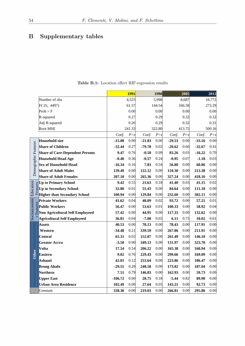
54 F. Clementi, V. Molini, and F. Schettino

B Supplementary tables

Table B.1: Location effect RIF-regression results

1991 1998 2005 2012

Number of obs 4,523 5,998 8,687 16,772

F( 25, 4497) 61.57 144.54 166.58 273.29

Prob > F 0.00 0.00 0.00 0.00

R-squared 0.27 0.29 0.32 0.32

Adj R-squared 0.26 0.29 0.32 0.31

Root MSE 241.33 322.80 413.75 500.16

Coef. P>z Coef. P>z Coef. P>z Coef. P>z

Dem

og

raph

ic F

eatu

res Household size -15.08 0.00 -21.83 0.00 -29.53 0.00 -33.16 0.00

Share of Children -32.44 0.27 -79.78 0.02 -20.62 0.60 -32.67 0.41

Share of Care-Dependent Persons 9.47 0.76 -0.58 0.99 83.26 0.03 -16.22 0.70

Household Head Age -0.40 0.36 -0.57 0.24 -0.95 0.07 -1.18 0.03

Sex of Household Head -16.34 0.16 7.83 0.54 56.80 0.00 60.86 0.00

Share of Adult Males 139.49 0.00 122.12 0.00 110.30 0.00 213.38 0.00

Share of Adult Females 207.10 0.00 265.36 0.00 327.24 0.00 418.16 0.00

Ed

uca

tio

n

Fea

ture

s Up to Primary School 9.42 0.55 21.63 0.18 41.40 0.03 41.15 0.02

Up to Secondary School 32.80 0.01 55.43 0.00 84.64 0.00 111.18 0.00

Higher than Secondary School 100.94 0.00 129.84 0.00 232.60 0.00 302.11 0.00

So

cio

eco

no

mi

c F

eatu

res Private Workers 41.62 0.04 48.09 0.02 93.72 0.00 57.21 0.01

Public Workers 56.47 0.00 53.63 0.01 100.33 0.00 58.92 0.04

Non Agricoltural Self Employeed 57.42 0.00 44.95 0.00 117.33 0.00 132.62 0.00

Agricoltural Self Employeed 36.81 0.04 -7.08 0.65 6.11 0.75 10.02 0.61

Oth

er

Assets 40.53 0.00 78.13 0.00 78.43 0.00 117.91 0.00

Western -34.48 0.21 339.59 0.00 267.86 0.00 211.91 0.00

Central 65.31 0.02 152.87 0.00 261.49 0.00 146.10 0.00

Greater Accra -3.50 0.90 349.13 0.00 131.97 0.00 323.70 0.00

Volta 17.54 0.54 206.22 0.00 165.38 0.00 160.94 0.00

Eastern 9.02 0.76 229.43 0.00 299.66 0.00 169.09 0.00

Ashanti 42.01 0.12 253.64 0.00 223.86 0.00 186.47 0.00

Brong Ahafo -29.55 0.28 248.58 0.00 173.82 0.00 187.04 0.00

Northern 7.51 0.79 146.83 0.00 162.93 0.00 59.73 0.00

Upper East -106.72 0.00 28.75 0.18 -5.44 0.82 89.90 0.00

Urban Area Residence 102.49 0.00 27.64 0.05 143.21 0.00 92.73 0.00

Constant 338.30 0.00 219.03 0.00 266.81 0.00 295.86 0.00

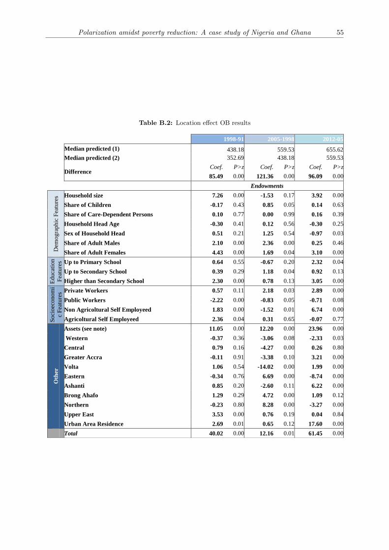
Polarization amidst poverty reduction: A case study of Nigeria and Ghana 55

Table B.2: Location effect OB results

1998-91 2005-1998 2012-05

Median predicted (1) 438.18 559.53 655.62

Median predicted (2) 352.69 438.18 559.53

Difference

Coef. P>z Coef. P>z Coef. P>z

85.49 0.00 121.36 0.00 96.09 0.00

Endowments

Dem

og

raph

ic F

eatu

res Household size 7.26 0.00 -1.53 0.17 3.92 0.00

Share of Children -0.17 0.43 0.85 0.05 0.14 0.63

Share of Care-Dependent Persons 0.10 0.77 0.00 0.99 0.16 0.39

Household Head Age -0.30 0.41 0.12 0.56 -0.30 0.25

Sex of Household Head 0.51 0.21 1.25 0.54 -0.97 0.03

Share of Adult Males 2.10 0.00 2.36 0.00 0.25 0.46

Share of Adult Females 4.43 0.00 1.69 0.04 3.10 0.00

Ed

uca

tio

n

Fea

ture

s Up to Primary School 0.64 0.55 -0.67 0.20 2.32 0.04

Up to Secondary School 0.39 0.29 1.18 0.04 0.92 0.13

Higher than Secondary School 2.30 0.00 0.78 0.13 3.05 0.00

So

cio

eco

no

mi

c F

eatu

res Private Workers 0.57 0.11 2.18 0.03 2.89 0.00

Public Workers -2.22 0.00 -0.83 0.05 -0.71 0.08

Non Agricoltural Self Employeed 1.83 0.00 -1.52 0.01 6.74 0.00

Agricoltural Self Employeed 2.36 0.04 0.31 0.65 -0.07 0.77

Oth

er

Assets (see note) 11.05 0.00 12.20 0.00 23.96 0.00

Western -0.37 0.36 -3.06 0.08 -2.33 0.03

Central 0.79 0.16 -4.27 0.00 0.26 0.80

Greater Accra -0.11 0.91 -3.38 0.10 3.21 0.00

Volta 1.06 0.54 -14.02 0.00 1.99 0.00

Eastern -0.34 0.76 6.69 0.00 -8.74 0.00

Ashanti 0.85 0.20 -2.60 0.11 6.22 0.00

Brong Ahafo 1.29 0.29 4.72 0.00 1.09 0.12

Northern -0.23 0.80 8.28 0.00 -3.27 0.00

Upper East 3.53 0.00 0.76 0.19 0.04 0.84

Urban Area Residence 2.69 0.01 0.65 0.12 17.60 0.00

Total 40.02 0.00 12.16 0.01 61.45 0.00

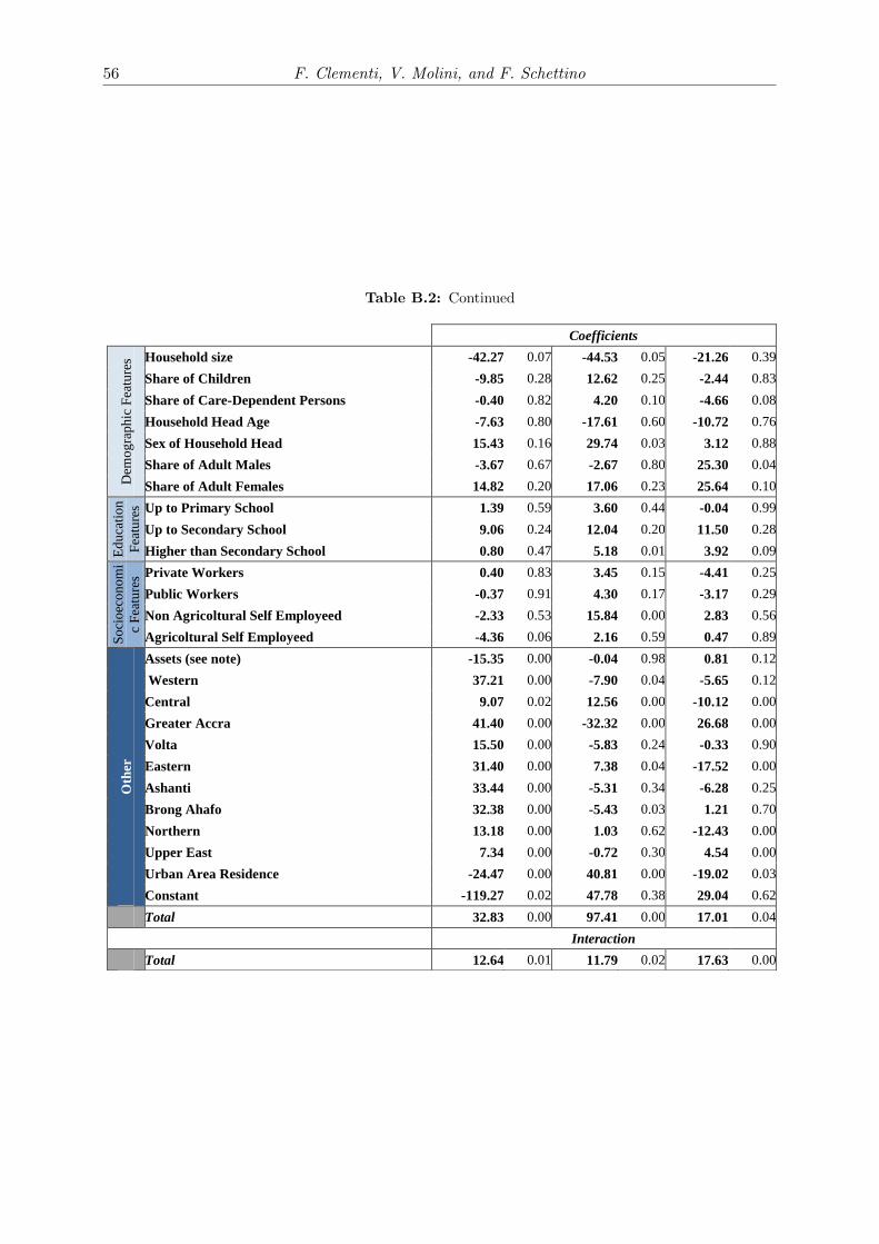
56 F. Clementi, V. Molini, and F. Schettino

Table B.2: Continued

Coefficients

Dem

og

raph

ic F

eatu

res Household size -42.27 0.07 -44.53 0.05 -21.26 0.39

Share of Children -9.85 0.28 12.62 0.25 -2.44 0.83

Share of Care-Dependent Persons -0.40 0.82 4.20 0.10 -4.66 0.08

Household Head Age -7.63 0.80 -17.61 0.60 -10.72 0.76

Sex of Household Head 15.43 0.16 29.74 0.03 3.12 0.88

Share of Adult Males -3.67 0.67 -2.67 0.80 25.30 0.04

Share of Adult Females 14.82 0.20 17.06 0.23 25.64 0.10

Ed

uca

tio

n

Fea

ture

s Up to Primary School 1.39 0.59 3.60 0.44 -0.04 0.99

Up to Secondary School 9.06 0.24 12.04 0.20 11.50 0.28

Higher than Secondary School 0.80 0.47 5.18 0.01 3.92 0.09

So

cio

eco

no

mi

c F

eatu

res Private Workers 0.40 0.83 3.45 0.15 -4.41 0.25

Public Workers -0.37 0.91 4.30 0.17 -3.17 0.29

Non Agricoltural Self Employeed -2.33 0.53 15.84 0.00 2.83 0.56

Agricoltural Self Employeed -4.36 0.06 2.16 0.59 0.47 0.89

Oth

er

Assets (see note) -15.35 0.00 -0.04 0.98 0.81 0.12

Western 37.21 0.00 -7.90 0.04 -5.65 0.12

Central 9.07 0.02 12.56 0.00 -10.12 0.00

Greater Accra 41.40 0.00 -32.32 0.00 26.68 0.00

Volta 15.50 0.00 -5.83 0.24 -0.33 0.90

Eastern 31.40 0.00 7.38 0.04 -17.52 0.00

Ashanti 33.44 0.00 -5.31 0.34 -6.28 0.25

Brong Ahafo 32.38 0.00 -5.43 0.03 1.21 0.70

Northern 13.18 0.00 1.03 0.62 -12.43 0.00

Upper East 7.34 0.00 -0.72 0.30 4.54 0.00

Urban Area Residence -24.47 0.00 40.81 0.00 -19.02 0.03

Constant -119.27 0.02 47.78 0.38 29.04 0.62

Total 32.83 0.00 97.41 0.00 17.01 0.04

Interaction

Total 12.64 0.01 11.79 0.02 17.63 0.00

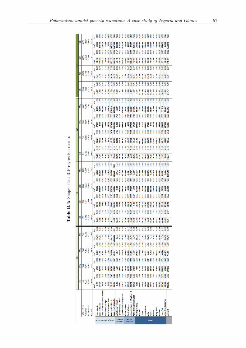
Polarization amidst poverty reduction: A case study of Nigeria and Ghana 57

Table

B.3:

Sh

ap

eeff

ect

RIF

-reg

ress

ion

resu

lts

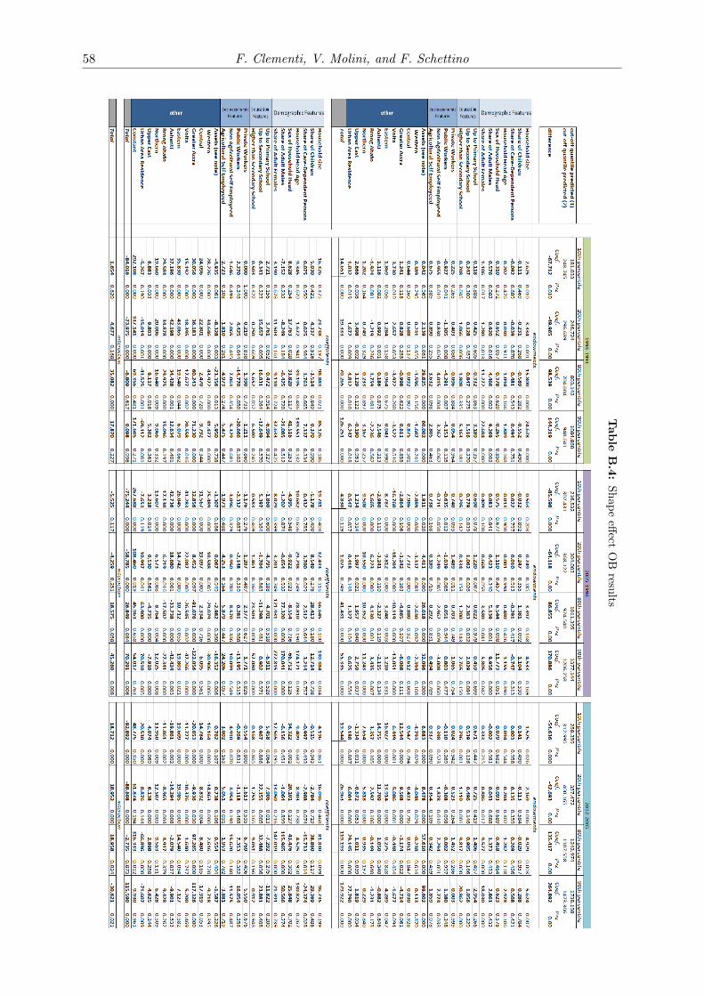
58 F. Clementi, V. Molini, and F. Schettino

Table

B.4:

Sh

ap

eeff

ectO

Bresu

lts