Embed Size (px)
Citation preview
POLARIS(Polarized Radiation Simulator)
User manual for POLARIS v4.03∗
Stefan Reissl1,3 and Robert Brauer2,3
1Heidelberg University, Institute for Theoretical Physics,Albert-Überle-Str. 2, 69120 Heidelberg, Germany
2CEA Saclay, DRF / IRFU / Service d’Astrophysique,Orme des Merisiers, 91191 Gif sur Yvette, France
3University of Kiel, Institute of Theoretical Physics and Astrophysics,
Leibnizstraße 15, 24118 Kiel, Germany
∗See Chapter 9 for the changelog of recent updates

Front page images
Oval panels: All-sky maps of intensity and degree of linear polarization of a post-processed SILCCsimulation provided by Philipp Girichidis.Squared panels: Degree of linear and circular polarization as well as line of sight magnetic fieldstrength of a post-processed MHD collapse simulation provided by Daniel Seifried.
Figure: Institutes that were or are still involved in the development of POLARIS. From left to right:Institute of Theoretical Physics and Astrophysics at the CAU Kiel (ITAP), the Center for Astronomy at theUniversity Heidelberg (ZAH), and the Institute of research into the fundamental laws of the Universe atCEA Saclay (IRFU).
1 Introduction
Apr., 1999 Development: MC3D in version 1 (basis for POLARIS, Wolf et al. 1999)
Feb., 2003 Development: MC3D in version 2 (basis for POLARIS, Wolf 2003)
2010 Development: MC3D in version 4 (basis for POLARIS)
2014 Development: Start of POLARIS development
June, 2014 Publication: Reissl et al. (2014)
July, 2015 Development: Mol3D (basis for line RT in POLARIS, Ober et al. 2015)
Apr., 2016 Publication: Brauer et al. (2016)
Sept., 2016 Publication: Reissl et al. (2016)
2017 Development: Final merge of MC3D and Mol3D into POLARIS
Sept., 2017 First POLARIS workshop in Heidelberg (website)
May, 2017 Publication: Brauer et al. (2017b)
July, 2017 Publication: Reissl et al. (2017)
Nov., 2017 Publication: Brauer et al. (2017a)
Mai, 2018 Publication: Reissl et al. (2018)
Aug., 2018 First public release of POLARIS
Jan., 2019 Publication: Seifried et al. (2019)
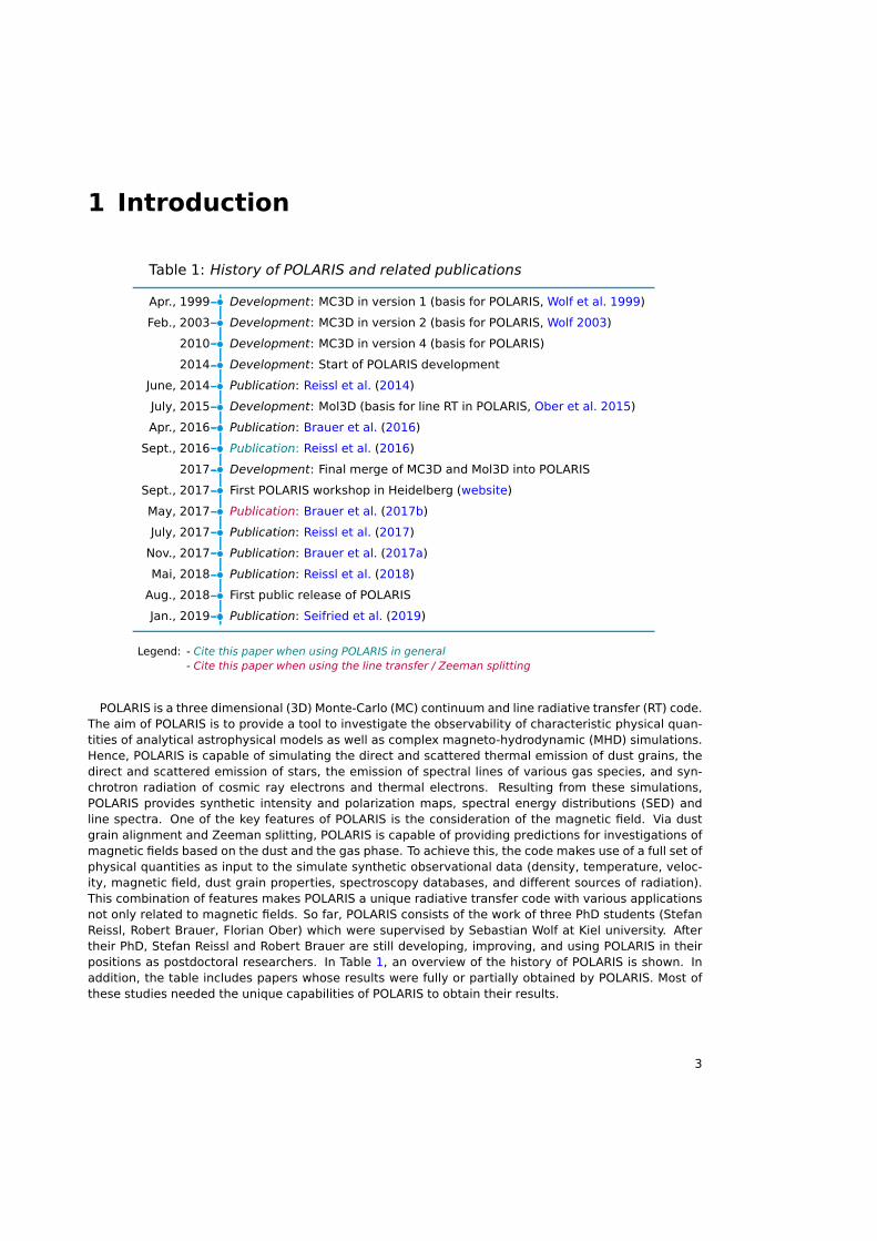
Table 1: History of POLARIS and related publications
Legend: - Cite this paper when using POLARIS in general- Cite this paper when using the line transfer / Zeeman splitting
POLARIS is a three dimensional (3D) Monte-Carlo (MC) continuum and line radiative transfer (RT) code.The aim of POLARIS is to provide a tool to investigate the observability of characteristic physical quan-tities of analytical astrophysical models as well as complex magneto-hydrodynamic (MHD) simulations.Hence, POLARIS is capable of simulating the direct and scattered thermal emission of dust grains, thedirect and scattered emission of stars, the emission of spectral lines of various gas species, and syn-chrotron radiation of cosmic ray electrons and thermal electrons. Resulting from these simulations,POLARIS provides synthetic intensity and polarization maps, spectral energy distributions (SED) andline spectra. One of the key features of POLARIS is the consideration of the magnetic field. Via dustgrain alignment and Zeeman splitting, POLARIS is capable of providing predictions for investigations ofmagnetic fields based on the dust and the gas phase. To achieve this, the code makes use of a full set ofphysical quantities as input to the simulate synthetic observational data (density, temperature, veloc-ity, magnetic field, dust grain properties, spectroscopy databases, and different sources of radiation).This combination of features makes POLARIS a unique radiative transfer code with various applicationsnot only related to magnetic fields. So far, POLARIS consists of the work of three PhD students (StefanReissl, Robert Brauer, Florian Ober) which were supervised by Sebastian Wolf at Kiel university. Aftertheir PhD, Stefan Reissl and Robert Brauer are still developing, improving, and using POLARIS in theirpositions as postdoctoral researchers. In Table 1, an overview of the history of POLARIS is shown. Inaddition, the table includes papers whose results were fully or partially obtained by POLARIS. Most ofthese studies needed the unique capabilities of POLARIS to obtain their results.
3
1 Introduction
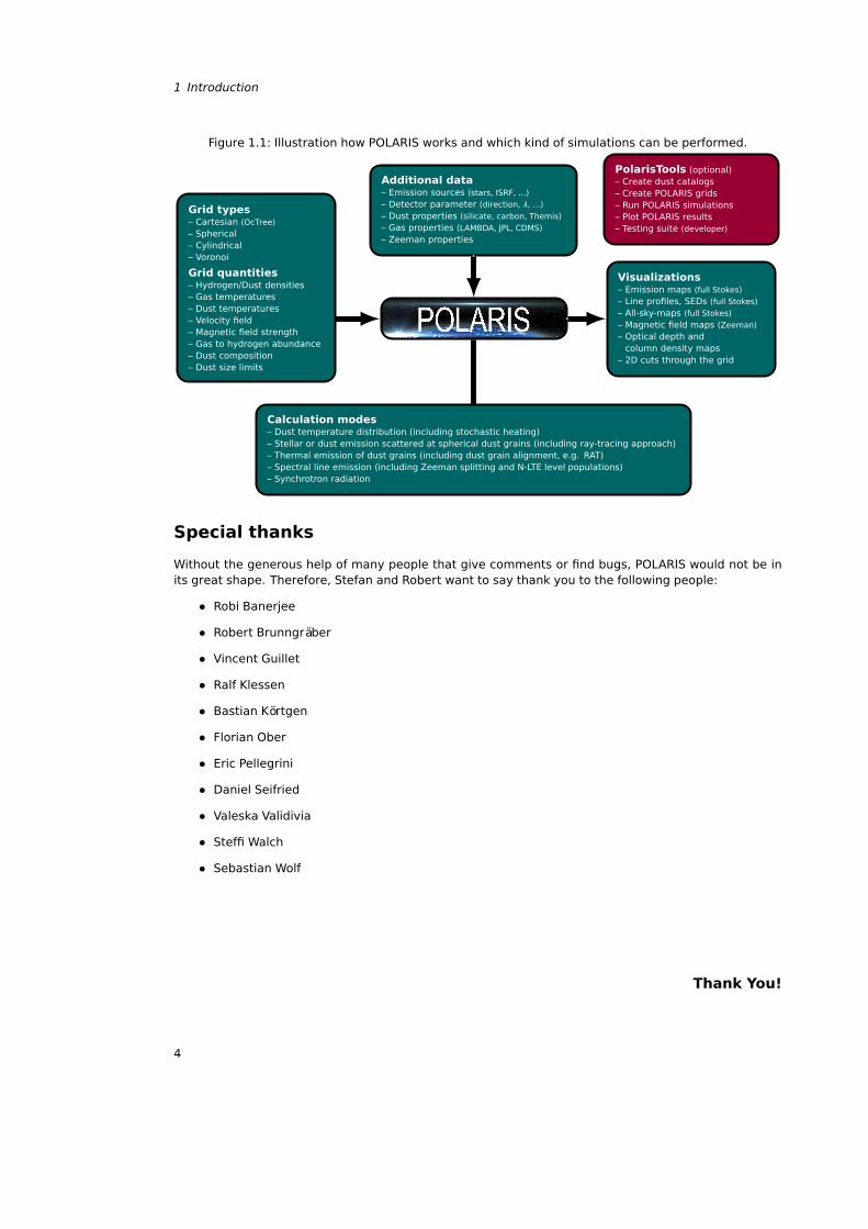
Figure 1.1: Illustration how POLARIS works and which kind of simulations can be performed.
Additional data– Emission sources (stars, ISRF, ...)
– Detector parameter (direction, λ, ...)
– Dust properties (silicate, carbon, Themis)
– Gas properties (LAMBDA, JPL, CDMS)
– Zeeman properties
Grid types– Cartesian (OcTree)
– Spherical– Cylindrical– Voronoi
Grid quantities– Hydrogen/Dust densities– Gas temperatures– Dust temperatures– Velocity field– Magnetic field strength– Gas to hydrogen abundance– Dust composition– Dust size limits
Calculation modes– Dust temperature distribution (including stochastic heating)– Stellar or dust emission scattered at spherical dust grains (including ray-tracing approach)– Thermal emission of dust grains (including dust grain alignment, e.g. RAT)– Spectral line emission (including Zeeman splitting and N-LTE level populations)– Synchrotron radiation
Visualizations– Emission maps (full Stokes)
– Line profiles, SEDs (full Stokes)
– All-sky-maps (full Stokes)
– Magnetic field maps (Zeeman)
– Optical depth andcolumn density maps
– 2D cuts through the grid
PolarisTools (optional)– Create dust catalogs– Create POLARIS grids– Run POLARIS simulations– Plot POLARIS results– Testing suite (developer)
Special thanks
Without the generous help of many people that give comments or find bugs, POLARIS would not be inits great shape. Therefore, Stefan and Robert want to say thank you to the following people:
• Robi Banerjee
• Robert Brunngräber
• Vincent Guillet
• Ralf Klessen
• Bastian Körtgen
• Florian Ober
• Eric Pellegrini
• Daniel Seifried
• Valeska Validivia
• Steffi Walch
• Sebastian Wolf
Thank You!
4

Copyright
The code is free of charge for any scientific purpose. This software is provided in the hope that it willbe useful but without any warranty of ability or fitness of a particular purpose. We also reject anyresponsibility for incorrect result that may be result from this code. Any publication that makes use ofthe software package (completely or in part) must mention the name of the POLARIS code and cite thePOLARIS paper(-s) as shown in Table 1.
5

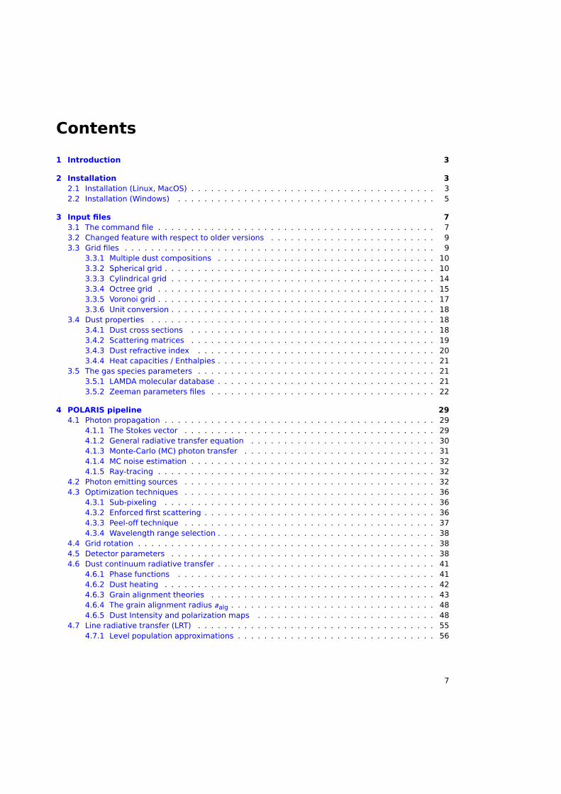
Contents
1 Introduction 3
2 Installation 32.1 Installation (Linux, MacOS) . . . . . . . . . . . . . . . . . . . . . . . . . . . . . . . . . . . . . 32.2 Installation (Windows) . . . . . . . . . . . . . . . . . . . . . . . . . . . . . . . . . . . . . . . 5
3 Input files 73.1 The command file . . . . . . . . . . . . . . . . . . . . . . . . . . . . . . . . . . . . . . . . . . 73.2 Changed feature with respect to older versions . . . . . . . . . . . . . . . . . . . . . . . . . 93.3 Grid files . . . . . . . . . . . . . . . . . . . . . . . . . . . . . . . . . . . . . . . . . . . . . . . 9
3.3.1 Multiple dust compositions . . . . . . . . . . . . . . . . . . . . . . . . . . . . . . . . . 103.3.2 Spherical grid . . . . . . . . . . . . . . . . . . . . . . . . . . . . . . . . . . . . . . . . . 103.3.3 Cylindrical grid . . . . . . . . . . . . . . . . . . . . . . . . . . . . . . . . . . . . . . . . 143.3.4 Octree grid . . . . . . . . . . . . . . . . . . . . . . . . . . . . . . . . . . . . . . . . . . 153.3.5 Voronoi grid . . . . . . . . . . . . . . . . . . . . . . . . . . . . . . . . . . . . . . . . . . 173.3.6 Unit conversion . . . . . . . . . . . . . . . . . . . . . . . . . . . . . . . . . . . . . . . . 18
3.4 Dust properties . . . . . . . . . . . . . . . . . . . . . . . . . . . . . . . . . . . . . . . . . . . 183.4.1 Dust cross sections . . . . . . . . . . . . . . . . . . . . . . . . . . . . . . . . . . . . . 183.4.2 Scattering matrices . . . . . . . . . . . . . . . . . . . . . . . . . . . . . . . . . . . . . 193.4.3 Dust refractive index . . . . . . . . . . . . . . . . . . . . . . . . . . . . . . . . . . . . 203.4.4 Heat capacities / Enthalpies . . . . . . . . . . . . . . . . . . . . . . . . . . . . . . . . . 21
3.5 The gas species parameters . . . . . . . . . . . . . . . . . . . . . . . . . . . . . . . . . . . . 213.5.1 LAMDA molecular database . . . . . . . . . . . . . . . . . . . . . . . . . . . . . . . . . 213.5.2 Zeeman parameters files . . . . . . . . . . . . . . . . . . . . . . . . . . . . . . . . . . 22
4 POLARIS pipeline 294.1 Photon propagation . . . . . . . . . . . . . . . . . . . . . . . . . . . . . . . . . . . . . . . . . 29
4.1.1 The Stokes vector . . . . . . . . . . . . . . . . . . . . . . . . . . . . . . . . . . . . . . 294.1.2 General radiative transfer equation . . . . . . . . . . . . . . . . . . . . . . . . . . . . 304.1.3 Monte-Carlo (MC) photon transfer . . . . . . . . . . . . . . . . . . . . . . . . . . . . . 314.1.4 MC noise estimation . . . . . . . . . . . . . . . . . . . . . . . . . . . . . . . . . . . . . 324.1.5 Ray-tracing . . . . . . . . . . . . . . . . . . . . . . . . . . . . . . . . . . . . . . . . . . 32
4.2 Photon emitting sources . . . . . . . . . . . . . . . . . . . . . . . . . . . . . . . . . . . . . . 324.3 Optimization techniques . . . . . . . . . . . . . . . . . . . . . . . . . . . . . . . . . . . . . . 36
4.3.1 Sub-pixeling . . . . . . . . . . . . . . . . . . . . . . . . . . . . . . . . . . . . . . . . . 364.3.2 Enforced first scattering . . . . . . . . . . . . . . . . . . . . . . . . . . . . . . . . . . . 364.3.3 Peel-off technique . . . . . . . . . . . . . . . . . . . . . . . . . . . . . . . . . . . . . . 374.3.4 Wavelength range selection . . . . . . . . . . . . . . . . . . . . . . . . . . . . . . . . . 38
4.4 Grid rotation . . . . . . . . . . . . . . . . . . . . . . . . . . . . . . . . . . . . . . . . . . . . . 384.5 Detector parameters . . . . . . . . . . . . . . . . . . . . . . . . . . . . . . . . . . . . . . . . 384.6 Dust continuum radiative transfer . . . . . . . . . . . . . . . . . . . . . . . . . . . . . . . . . 41
4.6.1 Phase functions . . . . . . . . . . . . . . . . . . . . . . . . . . . . . . . . . . . . . . . 414.6.2 Dust heating . . . . . . . . . . . . . . . . . . . . . . . . . . . . . . . . . . . . . . . . . 424.6.3 Grain alignment theories . . . . . . . . . . . . . . . . . . . . . . . . . . . . . . . . . . 434.6.4 The grain alignment radius aalg . . . . . . . . . . . . . . . . . . . . . . . . . . . . . . . 484.6.5 Dust Intensity and polarization maps . . . . . . . . . . . . . . . . . . . . . . . . . . . 48
4.7 Line radiative transfer (LRT) . . . . . . . . . . . . . . . . . . . . . . . . . . . . . . . . . . . . 554.7.1 Level population approximations . . . . . . . . . . . . . . . . . . . . . . . . . . . . . . 56
7
Contents
4.7.2 LRT with Zeeman effect . . . . . . . . . . . . . . . . . . . . . . . . . . . . . . . . . . . 574.8 Synchrotron RT . . . . . . . . . . . . . . . . . . . . . . . . . . . . . . . . . . . . . . . . . . . 61
4.8.1 CR electrons . . . . . . . . . . . . . . . . . . . . . . . . . . . . . . . . . . . . . . . . . 614.8.2 Thermal electrons . . . . . . . . . . . . . . . . . . . . . . . . . . . . . . . . . . . . . . 634.8.3 Synchrotron run with both electrons species . . . . . . . . . . . . . . . . . . . . . . . 64
5 Output data 675.1 Output grids . . . . . . . . . . . . . . . . . . . . . . . . . . . . . . . . . . . . . . . . . . . . . 675.2 Detector files . . . . . . . . . . . . . . . . . . . . . . . . . . . . . . . . . . . . . . . . . . . . 675.3 Gnuplot . . . . . . . . . . . . . . . . . . . . . . . . . . . . . . . . . . . . . . . . . . . . . . . 735.4 AMIRA . . . . . . . . . . . . . . . . . . . . . . . . . . . . . . . . . . . . . . . . . . . . . . . . 77
6 Quickstart guide 796.0.1 Unpack the examples . . . . . . . . . . . . . . . . . . . . . . . . . . . . . . . . . . . . 796.0.2 Dust temperature distribution . . . . . . . . . . . . . . . . . . . . . . . . . . . . . . . 796.0.3 Dust thermal emission . . . . . . . . . . . . . . . . . . . . . . . . . . . . . . . . . . . . 816.0.4 Dust thermal emission (with grain alignment) . . . . . . . . . . . . . . . . . . . . . . . 816.0.5 Scattered stellar emission . . . . . . . . . . . . . . . . . . . . . . . . . . . . . . . . . . 816.0.6 Thermal emission and scattered stellar emission . . . . . . . . . . . . . . . . . . . . . 816.0.7 Spectral line emission . . . . . . . . . . . . . . . . . . . . . . . . . . . . . . . . . . . . 816.0.8 Spectral line emission (with Zeeman splitting) . . . . . . . . . . . . . . . . . . . . . . 82
7 PolarisTools 837.1 Introduction . . . . . . . . . . . . . . . . . . . . . . . . . . . . . . . . . . . . . . . . . . . . . 837.2 The command polaris-gen . . . . . . . . . . . . . . . . . . . . . . . . . . . . . . . . . . . . . 847.3 The command polaris-run . . . . . . . . . . . . . . . . . . . . . . . . . . . . . . . . . . . . . 847.4 The command polaris-plot . . . . . . . . . . . . . . . . . . . . . . . . . . . . . . . . . . . . . 877.5 The command polaris-remote . . . . . . . . . . . . . . . . . . . . . . . . . . . . . . . . . . . 957.6 The command polaris-extra . . . . . . . . . . . . . . . . . . . . . . . . . . . . . . . . . . . . 957.7 Available choices . . . . . . . . . . . . . . . . . . . . . . . . . . . . . . . . . . . . . . . . . . 987.8 Create your own project . . . . . . . . . . . . . . . . . . . . . . . . . . . . . . . . . . . . . . 103
7.8.1 Creating a model . . . . . . . . . . . . . . . . . . . . . . . . . . . . . . . . . . . . . . . 1037.8.2 Creating a gas species . . . . . . . . . . . . . . . . . . . . . . . . . . . . . . . . . . . . 1037.8.3 Creating a dust component . . . . . . . . . . . . . . . . . . . . . . . . . . . . . . . . . 1037.8.4 Creating a detector . . . . . . . . . . . . . . . . . . . . . . . . . . . . . . . . . . . . . 1077.8.5 Creating a stellar radiation source . . . . . . . . . . . . . . . . . . . . . . . . . . . . . 1077.8.6 Creating a background radiation source . . . . . . . . . . . . . . . . . . . . . . . . . . 1077.8.7 Creating a custom plot routine . . . . . . . . . . . . . . . . . . . . . . . . . . . . . . . 1077.8.8 Adding a server/cluster . . . . . . . . . . . . . . . . . . . . . . . . . . . . . . . . . . . 1147.8.9 Creating an external input . . . . . . . . . . . . . . . . . . . . . . . . . . . . . . . . . 114
7.9 Quickstart guide . . . . . . . . . . . . . . . . . . . . . . . . . . . . . . . . . . . . . . . . . . . 1167.9.1 Create a grid . . . . . . . . . . . . . . . . . . . . . . . . . . . . . . . . . . . . . . . . . 1167.9.2 Dust temperature distribution . . . . . . . . . . . . . . . . . . . . . . . . . . . . . . . 1167.9.3 Dust thermal emission . . . . . . . . . . . . . . . . . . . . . . . . . . . . . . . . . . . . 1167.9.4 Dust thermal emission (with grain alignment) . . . . . . . . . . . . . . . . . . . . . . . 1197.9.5 Scattered stellar emission . . . . . . . . . . . . . . . . . . . . . . . . . . . . . . . . . . 1197.9.6 Thermal emission and scattered stellar emission . . . . . . . . . . . . . . . . . . . . . 1197.9.7 Spectral line emission . . . . . . . . . . . . . . . . . . . . . . . . . . . . . . . . . . . . 1217.9.8 Spectral line emission (with Zeeman splitting) . . . . . . . . . . . . . . . . . . . . . . 121
8 Files and directories 123
9 Changelog 125
Index 127
1

2 Installation
2.1 Installation (Linux, MacOS)
Download
The POLARIS installation package can be downloaded from [here].
Requirements
The following packages are required for the installation:
• cmake
• GNU Compiler Collection (gcc) with OpenMP support
(Linux server/cluster user only) Some linux servers have not a recent version of gcc with OpenMP supportinstalled. However, most server/cluster systems offer the use of environment modules to update to arecent version of gcc or OpenMP. Information about the usage can be found online.(Mac user only) The installation of gcc with OpenMP support can be done by using Homebrew and enteringthe following command:
brew install gcc --without-multilib
The then installed gcc compiler can usually be found as gcc-X, where X is the version number. To usethis compiler for the POLARIS installation on your Mac, the alias function can be used as follows:
alias gcc=gcc-X
Installation
To install POLARIS on your computer, open a terminal/console and go into the directory where youdownloaded 'polaris.run'. Then, by entering the following command, POLARIS will be installed in thecurrent directory:
./polaris.run
If the package is not executable, enter the following command in advance:
chmod +x polaris.run
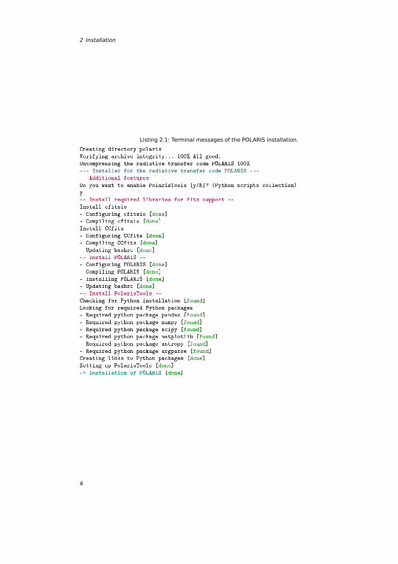
The POLARIS package will extract itself into a newly created polaris/ directory and the terminal mes-sages of the installation should look like Listing 2.1. POLARIS and PolarisTools (if chosen) can now beexecuted from any newly opened terminal/console. However, to use it in already open terminals/con-soles, execute the following command to update the environmental paths:
source ~/.bashrc
(PolarisTools only) If Python needs to be installed by the install script, the subsequent installation mightquit with an error. In this case, execute the source command as described above and execute the installscript again by entering the following command:
./polaris/install_polaris.sh
→ If you want perform your first simulations as quickly as possible, go directly to Sect. 6 (usingcommand files) or Sect. 7.9 (using PolarisTools).→ If you already worked with a previous version of POLARIS by using command files, go directly to
Sect. 3.2 to see how to adapt your command files to the current version of POLARIS.
3
2 Installation
Listing 2.1: Terminal messages of the POLARIS installation.
Creating directory polaris
Verifying archive integrity... 100% All good.
Uncompressing the radiative transfer code POLARIS 100%
Installer for the radiative transfer code POLARIS
- Additional features -
Do you want to enable PolarisTools [y/N]? (Python scripts collection)
y
- Install required libraries for fits support -
Install cfitsio
- Configuring cfitsio [done]
- Compiling cfitsio [done]
Install CCfits
- Configuring CCfits [done]
- Compiling CCfits [done]
- Updating bashrc [done]
- Install POLARIS -
- Configuring POLARIS [done]
- Compiling POLARIS [done]
- Installing POLARIS [done]
- Updating bashrc [done]
- Install PolarisTools -
Checking for Python installation [found]
Looking for required Python packages
- Required python package pandas [found]
- Required python package numpy [found]
- Required python package scipy [found]
- Required python package matplotlib [found]
- Required python package astropy [found]
- Required python package argparse [found]
Creating links to Python packages [done]
Setting up PolarisTools [done]
-> Installation of POLARIS [done]
4
2.2 Installation (Windows)
Options of the installation script
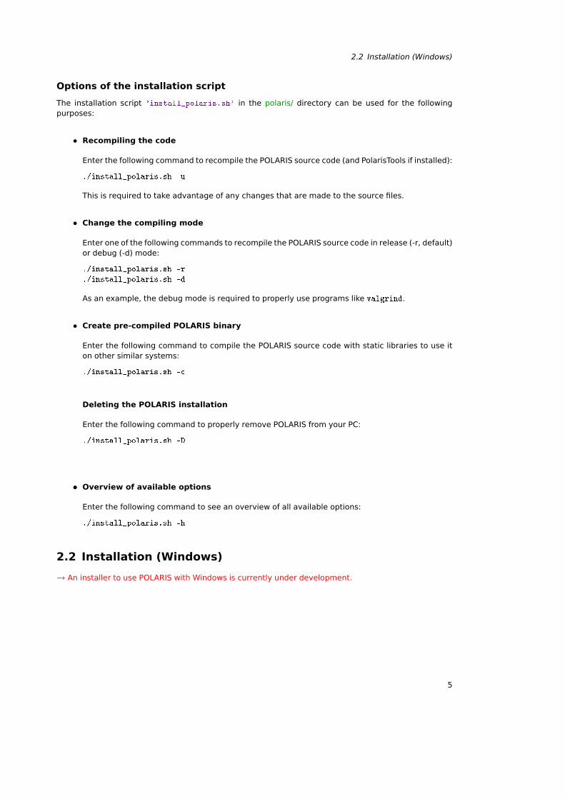
The installation script 'install_polaris.sh' in the polaris/ directory can be used for the followingpurposes:
• Recompiling the code
Enter the following command to recompile the POLARIS source code (and PolarisTools if installed):
./install_polaris.sh -u
This is required to take advantage of any changes that are made to the source files.
• Change the compiling mode
Enter one of the following commands to recompile the POLARIS source code in release (-r, default)or debug (-d) mode:
./install_polaris.sh -r
./install_polaris.sh -d
As an example, the debug mode is required to properly use programs like valgrind.
• Create pre-compiled POLARIS binary
Enter the following command to compile the POLARIS source code with static libraries to use iton other similar systems:
./install_polaris.sh -c
Deleting the POLARIS installation
Enter the following command to properly remove POLARIS from your PC:
./install_polaris.sh -D
•• Overview of available options
Enter the following command to see an overview of all available options:
./install_polaris.sh -h
2.2 Installation (Windows)
→ An installer to use POLARIS with Windows is currently under development.
5

3 Input files
3.1 The command file
A simulation with POLARIS can be executed by providing the path to a command file as a single argu-ment:
polaris PATH/TO/THE/command_file
Predefined commands in a pseudo XML style are implemented in the code and allow the user to createa script with sequences of simulations. The structure of the command file is intended to be simple andsuggestive. A complete list of commands is provided in Tables 3.4 to 3.7 at the end of this section.
The POLARIS parser does not distinguish between tab and whitespace nor does it care about thenumber of tabs and whitespaces between each command. Lines marked with a # or a ! are ignored andcan be used as comments. The command file consists of an arbitrary number of tasks. Each task blockhas the following form:
<task> 0/1
# commands ...
</task>
The number 1 is optional. Task blocks with a 0 will be skipped completely. Commands that are commonto all tasks can be defined in an extra block in the beginning as the first block of the command file with:
<common> 0/1
# commands ...
</common>
When identical commands appear in both the common-block and in a task-block the command writtenin the task-block has priority. The order of commands inside each task block is mostly irrelevant. Ex-ceptions are gas species (see Sect. 4.7.2), background sources (see Sect. 4.2), and detectors (see Sect.4.5) which are numbered in the order of theirs appearance. Each task-block needs a command thatdefines the pipeline ID (simulation type). A detailed description of each simulation type is provided inChapt. 4.
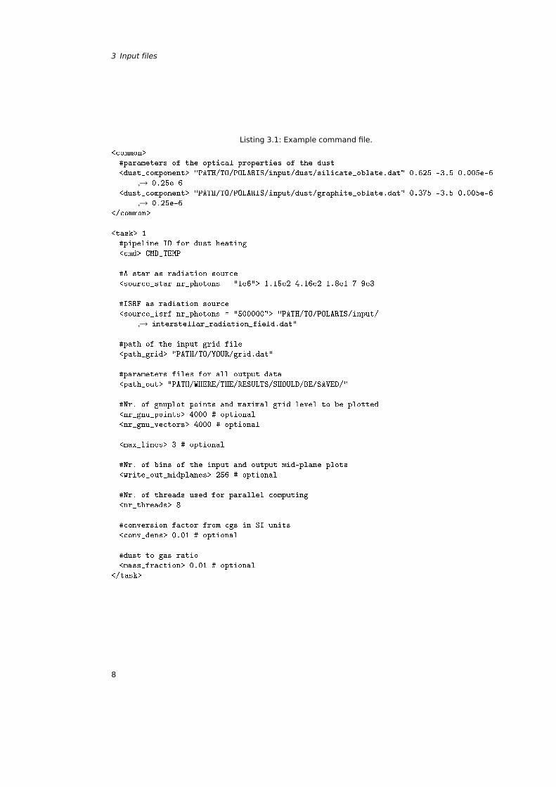
A command file example to perform the calculation of the dust temperature can be found in Listing 3.1In this example, the command CMD_TEMP runs a simulation for heating the dust by considering different
photon emitting sources (see Sect. 4.2). In this case, a single star and the interstellar radiation field(ISRF) are considered as sources. The ISRF source requires an external file for the spectral energy distri-bution (SED). In contrast to dust polarization and emission, the LRT (see Sect. 4.7) and the synchrotronruns do not require a dust model (see Sect. 4.8).
A dust model consists of a arbitrary number of grain material, mass fraction, size distribution, andsize ranges. In the above example the dust model is defined in the common block. In this particularcase a dust grain model mixture of 62.5% silicate and 37.5% graphite is used with an size distribution ofnd(a) ∝ a−3.5. The values 0.005 × 10⁻⁶ and 0.25 × 10⁻⁶ are the minimal and maximal dust grain radii inmeters. The available grain size range can be found in the dust parameters file (see Sect. 3.4). With<path_grid>, the path to the input grid is defined. Each simulation of a POLARIS pipeline requires a gridwith a set of physical input parameters in a predefined geometry. The units of the grid quantities needto be in SI units or in cgs units, if <path_grid_cgs> is used. The creation of such a grid is described inSect 3.3 in greater detail. With <path_out>, the path to the resulting output files is defined.POLARIS can plot the input and output 3D distributions of the physical parameters of a particular gridas gnuplot files. The next optional lines define the number of data points and vectors as well as the stepfor the grid lines to be plotted. Additionally, the values of the xy-, xz-, and yz - midplane files can bewritten as fits files in a regular raster.
7
3 Input files
Listing 3.1: Example command file.
<common>
#parameters of the optical properties of the dust
<dust_component> "PATH/TO/POLARIS/input/dust/silicate_oblate.dat" 0.625 -3.5 0.005e-6
→ 0.25e-6
<dust_component> "PATH/TO/POLARIS/input/dust/graphite_oblate.dat" 0.375 -3.5 0.005e-6
→ 0.25e-6
</common>
<task> 1
#pipeline ID for dust heating
<cmd> CMD_TEMP
#A star as radiation source
<source_star nr_photons = "1e6"> 1.15e2 4.16e2 1.8e1 7 9e3
#ISRF as radiation source
<source_isrf nr_photons = "500000"> "PATH/TO/POLARIS/input/
→ interstellar_radiation_field.dat"
#path of the input grid file
<path_grid> "PATH/TO/YOUR/grid.dat"
#parameters files for all output data
<path_out> "PATH/WHERE/THE/RESULTS/SHOULD/BE/SAVED/"
#Nr. of gnuplot points and maximal grid level to be plotted
<nr_gnu_points> 4000 # optional
<nr_gnu_vectors> 4000 # optional
<max_lines> 3 # optional
#Nr. of bins of the input and output mid-plane plots
<write_out_midplanes> 256 # optional
#Nr. of threads used for parallel computing
<nr_threads> 8
#conversion factor from cgs in SI units
<conv_dens> 0.01 # optional
#dust to gas ratio
<mass_fraction> 0.01 # optional
</task>
8
3.2 Changed feature with respect to older versions
Hence, the command <write_out_midplanes> defines the resolution of the mid-plane files with pre-defined number of bins (e.g. 256). In POLARIS the problem of radiative transfer is solved in a par-allelized way using the OpenMP library. The number of processors can be defined with the com-mand <nr_threads>. POLARIS works internally strictly in SI unity for all input parameters. Physicalquantities predefined in the grid need possibly to be converted (see Sect. 3.3.6 for details). With<conv_dens> 0.01, the grid density is converted from cgs in SI. Finally, the dust-to-gas mass ratio isdefined by <mass_fraction>. If the <mass_fraction> is set to zero, the fractions of the dust componentsare used instead and do not have to be summed up to one (see Sect. 4.6.5).
This sample script is just a general overview. A detailed description of the manifold features of PO-LARIS and the corresponding commands to control them is provided in the following sections.
HINTS:
• No extra directory needs to be created in advance. POLARIS creates automatically all thenecessary directories defined by the output path.
• All paths have to be written in quotation marks.
3.2 Changed feature with respect to older versions
The version 4.00 is the first public release of the POLARIS code. In order to keep consistency we re-named some of the commands. However, people used previous versions for their projects and publica-tions (versions less than 4.00). Hence, we give a short list of changed commands in Tab. 3.1.
Table 3.1: List of commands that changed compared to previous versions
previously current version
CMD_RAYTRACING CMD_DUST_EMISSION
CMD_MCPOL CMD_DUST_SCATTERING
CMD_LINETRANSFER CMD_LINE_EMISSION
<plot_inp_midplanes> no longer exists
<plot_out_midplanes> no longer exists
all of the detector commands see Sect. 4.5
<gas_species vel_channels = > max_vel and vel_channels moved to detector
wavelengths & grain sizes moved from indices to physical values in SI
3.3 Grid files
In POLARIS RT simulations can be performed with four different grid geometries so far. The availablegrid types are spherical, cylindrical, octree, and Voronoi. All the grids have in common that they startwith a standardized header followed by a grid specific data section. All quantities are stored in a binaryformat.
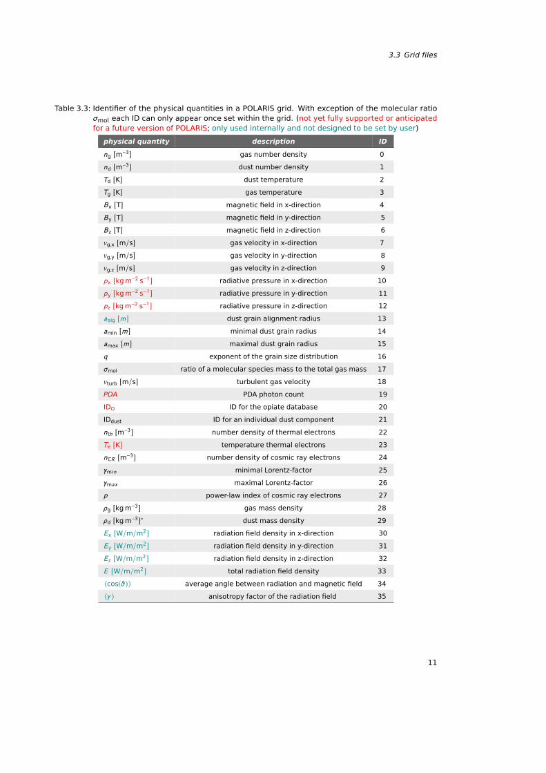
The grid type itself is characterized by IDgrid (unsigned short, 2 bytes) which is the very first numberin each grid file is shown in Table 3.2. After the grid IDgrid follows a number Nphys (unsigned short, 2bytes) that defines the amount of physical quantities for each grid cell and a list of IDs (unsigned short, 2bytes) to identify each quantity (see Tab 3.3). With exception of ng/ρg, nd/ρd,Td, and nmol all identifierscan only appear once in the header. POLARIS RT simulations require at least a gas density ng/ρg asphysical quantity in each grid cell. All other quantities are optional and depend on the kind of chosensimulation pipeline (see Chapt. 4). Instead of number densities n, mass densities ρ of the gas and dustcan be defined as well. However, a grid cannot be used, if densities of both units are defined.
9
3 Input files
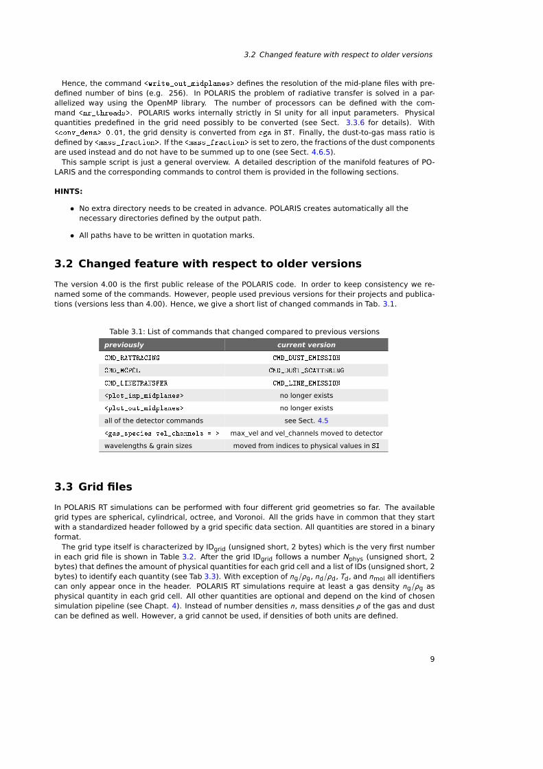
Table 3.2: IDs for the implemented POLARIS grid types.
type octree spherical cylindrical voronoi
IDgrid 20 30 40 50
3.3.1 Multiple dust compositions
There are two different methods to define the distribution of multiple dust compositions inside of thegrid. Either the dust mixture index IDdust is set for each grid cell or multiple dust density distributions(or gas densities via gas-to-dust mass ratio) are defined. With the first method, the radiative transferis performed by using in each cell the dust composition related to the set IDdust (see 4.6.5 for definingmultiple dust compositions). This is the suggested method for grids based on MHD/HD simulations, sincethey usually are only supporting one density distribution and adding an additional value to each cell iseasily realized. A more sophisticated approach is the usage of multiple density distributions (nd/ρdor ng/ρg). For this method, the user needs to define as much dust compositions as there are densitydistributions. With this, the radiative transfer is performed by using in each cell a mixture of the dustcompositions that depends on the ratio between all density distributions. This method is well suited forgrids based on analytical models since multiple density distributions can easily created analytically.
HINTS:
• If you want a specific cell to be skipped in a RT simulation set its density to zero.
• POLARIS shifts the center of the grid to be in the center of the external coordinate system. Thecoordinates of the radiating sources (see Sect. 4.2) have possibly to be adapted accordingly!
3.3.2 Spherical grid
After defining the header, the spherical grid can be defined by an additional sequence of 8 numbersRmin, Rmax, Nr, Nϕ , Nϑ , fr, fϕ , fϑ . Here, the first two, Rmin and Rmax, respectively, define the in-ner and outer radius of the sphere followed by the number of cells in r-direction Nr, ϕ-direction Nϕ ,and ϑ-direction Nϑ , respectively. The boundary of the grid is a sphere with a radius of Rmax. The shapeparameter fr, fϕ , and fϑ determine the distribution of steps along the r-direction and the ϑ-direction with:
Radial direction
• fr = 0The header has to be followed by Nr−1 values (double, 8 bytes) that define the location of each i -th radial cell border with r2 < · · · < ri−1 < ri < ri+1 < · · · < rNr whereas r1 = Rmin and rNr+1 = Rmax,respectively.
• fr < 0The cell borders along the r-direction are equally distributed to create Nr cells.
• fr = 1The i -th cell border in the r-direction is calculated according to:
ri = Rmin + (Rmax − Rmin) sin
(i π
Nr
). (3.1)
• fr > 1The i -th cell border in the r-direction is calculated according to:
ri = Rmax +(f ir − 1)(Rmax − Rmin)
f Nrr − 1
. (3.2)
10
3.3 Grid files
Table 3.3: Identifier of the physical quantities in a POLARIS grid. With exception of the molecular ratioσmol each ID can only appear once set within the grid. (not yet fully supported or anticipatedfor a future version of POLARIS; only used internally and not designed to be set by user)
physical quantity description ID
ng [m−3] gas number density 0
nd [m−3] dust number density 1
Td [K] dust temperature 2
Tg [K] gas temperature 3
Bx [T] magnetic field in x-direction 4
By [T] magnetic field in y-direction 5
Bz [T] magnetic field in z-direction 6
vg,x [m/s] gas velocity in x-direction 7
vg,y [m/s] gas velocity in y-direction 8
vg,z [m/s] gas velocity in z-direction 9
px [kg m−2 s−1] radiative pressure in x-direction 10
py [kg m−2 s−1] radiative pressure in y-direction 11
pz [kg m−2 s−1] radiative pressure in z-direction 12
aalg [m] dust grain alignment radius 13
amin [m] minimal dust grain radius 14
amax [m] maximal dust grain radius 15
q exponent of the grain size distribution 16
σmol ratio of a molecular species mass to the total gas mass 17
vturb [m/s] turbulent gas velocity 18
PDA PDA photon count 19
IDO ID for the opiate database 20
IDdust ID for an individual dust component 21
nth [m−3] number density of thermal electrons 22
Te [K] temperature thermal electrons 23
nCR [m−3] number density of cosmic ray electrons 24
γmi n minimal Lorentz-factor 25
γmax maximal Lorentz-factor 26
p power-law index of cosmic ray electrons 27
ρg [kg m−3] gas mass density 28
ρd [kg m−3]∗ dust mass density 29
Ex [W/m/m2] radiation field density in x-direction 30
Ey [W/m/m2] radiation field density in y-direction 31
Ez [W/m/m2] radiation field density in z-direction 32
E [W/m/m2] total radiation field density 33
〈cos(ϑ)〉 average angle between radiation and magnetic field 34
〈γ 〉 anisotropy factor of the radiation field 35
11
3 Input files
-100
-50
0
50
100
-100-50 0 50 100-100
-50
0
50
100
z [AU]
1
2
3
4
5
6
7
8
9
10
11
12
13
14
15
16
17
x [AU]
y [AU]
z [AU]
-0.4-0.2
0 0.2
0.4
-0.4
-0.2
0
0.2
0.4
-0.4
-0.2
0
0.2
0.4
z [pc]
1
2
3
4
5
6
7
8
9
10
11
12
13
14
15
16
17
18
19
20
21
22
23
24
25
26
x [pc]
y [pc]
z [pc]
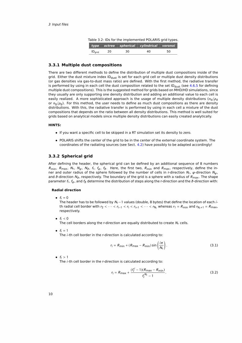
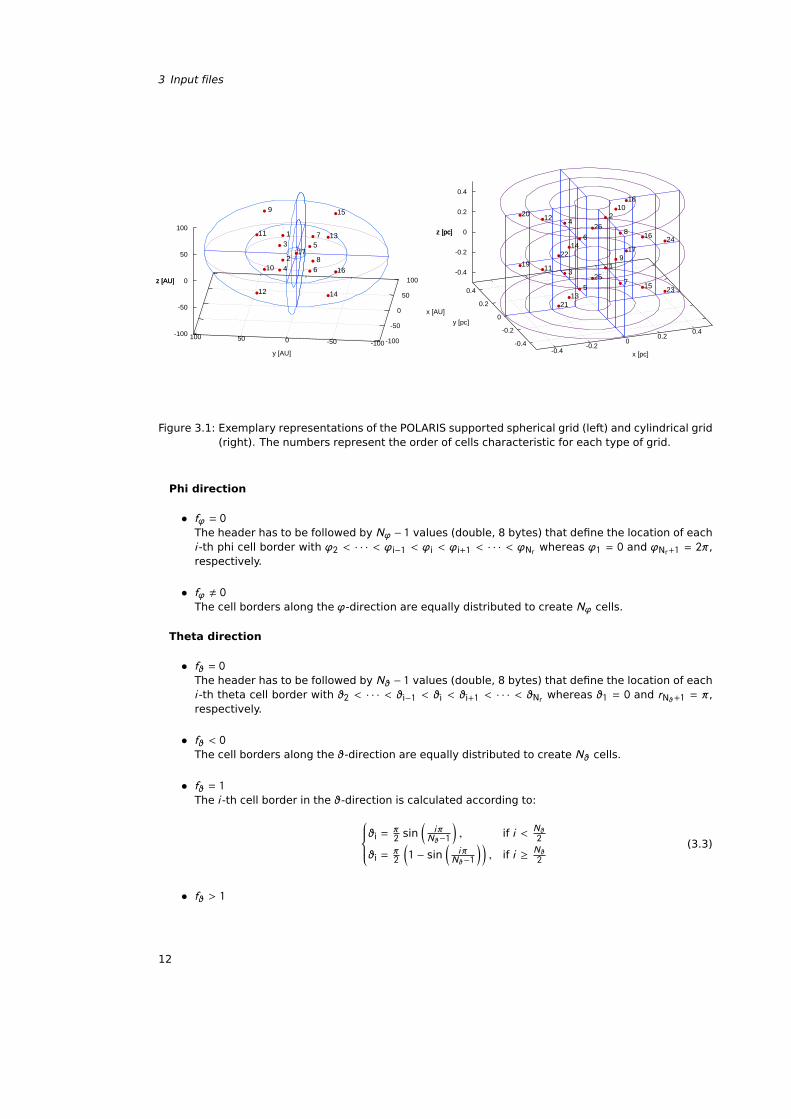
Figure 3.1: Exemplary representations of the POLARIS supported spherical grid (left) and cylindrical grid(right). The numbers represent the order of cells characteristic for each type of grid.
Phi direction
• fϕ = 0The header has to be followed by Nϕ − 1 values (double, 8 bytes) that define the location of eachi -th phi cell border with ϕ2 < · · · < ϕi−1 < ϕi < ϕi+1 < · · · < ϕNr whereas ϕ1 = 0 and ϕNr+1 = 2π,respectively.
• fϕ , 0The cell borders along the ϕ-direction are equally distributed to create Nϕ cells.
Theta direction
• fϑ = 0The header has to be followed by Nϑ − 1 values (double, 8 bytes) that define the location of eachi -th theta cell border with ϑ2 < · · · < ϑi−1 < ϑi < ϑi+1 < · · · < ϑNr whereas ϑ1 = 0 and rNϑ+1 = π,respectively.
• fϑ < 0The cell borders along the ϑ-direction are equally distributed to create Nϑ cells.
• fϑ = 1The i -th cell border in the ϑ-direction is calculated according to:
ϑi =π2 sin
(i πNϑ−1
), if i < Nϑ
2
ϑi =π2
(1 − sin
(i πNϑ−1
)), if i ≥ Nϑ
2
(3.3)
• fϑ > 1
12
3.3 Grid files
The i -th cell border in the ϑ-direction is calculated according to:ϑi =
π2 −
(fNϑ2 −i
ϑ−1) π2
f
Nϑ2
ϑ−1, if i < Nϑ
2
ϑi =π2 +
(f i−Nϑ2
ϑ−1) π2
f
Nϑ2
ϑ−1, if i ≥ Nϑ
2
(3.4)
If multiple shape parameters f are zero, the lists of cell borders have to be in the same order as theshape parameters itself. As for the order of cells the grid runs over ϑ, ϕ, and r. Hence the position ofeach cell within the grid is defined by its order of appearance in the grid file. The cell at the center is thelast cell in the list leading to a total amount of Nc = Nr × Nϕ × Nϑ + 1 cells. This gives for the sphericalgrid file the following form:
IDgrid (unsigned short, 2 bytes, 30 = spherical)Nphys (unsigned short, 2 bytes, maximal 21 possible physical quantities in each cell)IDng ... IDp (unsigned short, 2 bytes, optionally and in arbitrary order)Rmin Rmax (double, 8 bytes)Nr Nϕ Nϑ (unsigned short, 2 bytes)fr fϕ fϑ (double, 8 bytes)ng ... p (double, 8 bytes, in the same order as in the header, 1st cell)...ng ... p (double, 8 bytes, last outer cell, Nc − 1 − t h cell)ng ... p (double, 8 bytes, center cell, Nc − t h cell)
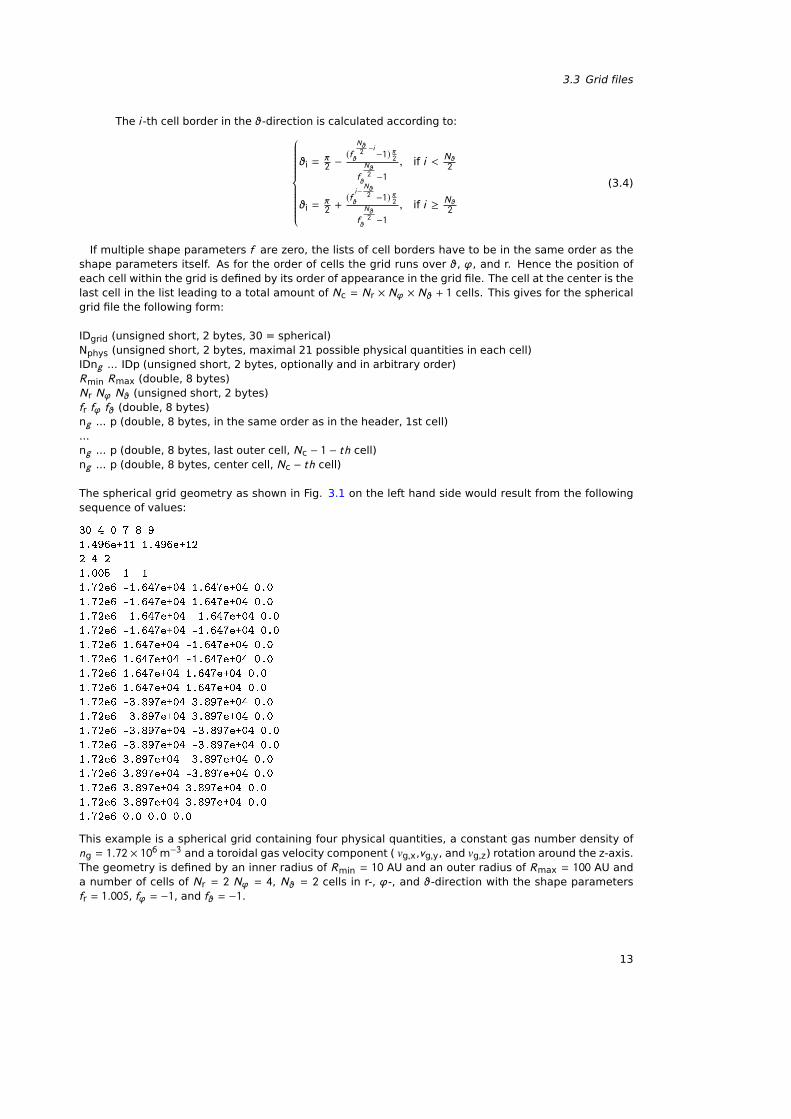
The spherical grid geometry as shown in Fig. 3.1 on the left hand side would result from the followingsequence of values:
30 4 0 7 8 9
1.496e+11 1.496e+12
2 4 2
1.005 -1 -1
1.72e6 -1.647e+04 1.647e+04 0.0
1.72e6 -1.647e+04 1.647e+04 0.0
1.72e6 -1.647e+04 -1.647e+04 0.0
1.72e6 -1.647e+04 -1.647e+04 0.0
1.72e6 1.647e+04 -1.647e+04 0.0
1.72e6 1.647e+04 -1.647e+04 0.0
1.72e6 1.647e+04 1.647e+04 0.0
1.72e6 1.647e+04 1.647e+04 0.0
1.72e6 -3.897e+04 3.897e+04 0.0
1.72e6 -3.897e+04 3.897e+04 0.0
1.72e6 -3.897e+04 -3.897e+04 0.0
1.72e6 -3.897e+04 -3.897e+04 0.0
1.72e6 3.897e+04 -3.897e+04 0.0
1.72e6 3.897e+04 -3.897e+04 0.0
1.72e6 3.897e+04 3.897e+04 0.0
1.72e6 3.897e+04 3.897e+04 0.0
1.72e6 0.0 0.0 0.0
This example is a spherical grid containing four physical quantities, a constant gas number density ofng = 1.72 × 10⁶ m−3 and a toroidal gas velocity component ( vg,x,vg,y, and vg,z) rotation around the z-axis.The geometry is defined by an inner radius of Rmin = 10 AU and an outer radius of Rmax = 100 AU anda number of cells of Nr = 2 Nϕ = 4, Nϑ = 2 cells in r-, ϕ-, and ϑ-direction with the shape parametersfr = 1.005, fϕ = −1, and fϑ = −1.
13
3 Input files
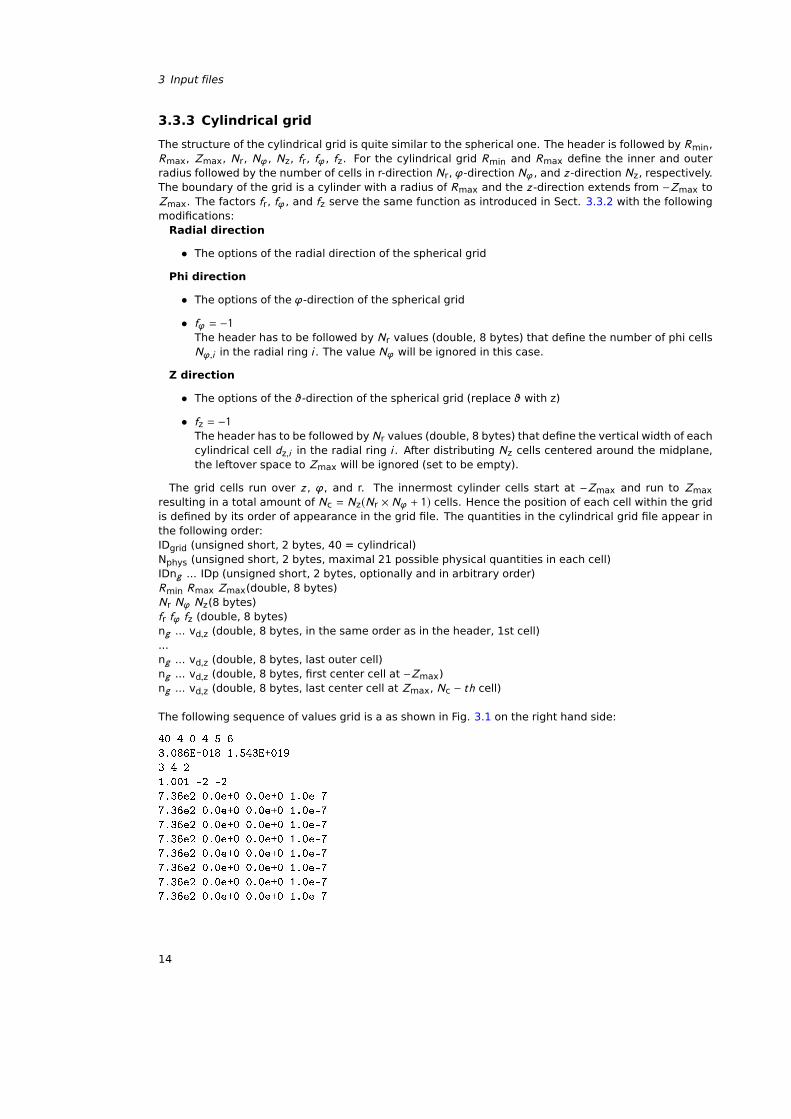
3.3.3 Cylindrical grid
The structure of the cylindrical grid is quite similar to the spherical one. The header is followed by Rmin,Rmax, Zmax, Nr, Nϕ , Nz, fr, fϕ , fz. For the cylindrical grid Rmin and Rmax define the inner and outerradius followed by the number of cells in r-direction Nr, ϕ-direction Nϕ , and z -direction Nz, respectively.The boundary of the grid is a cylinder with a radius of Rmax and the z -direction extends from −Zmax toZmax. The factors fr, fϕ , and fz serve the same function as introduced in Sect. 3.3.2 with the followingmodifications:
Radial direction
• The options of the radial direction of the spherical grid
Phi direction
• The options of the ϕ-direction of the spherical grid
• fϕ = −1The header has to be followed by Nr values (double, 8 bytes) that define the number of phi cellsNϕ,i in the radial ring i . The value Nϕ will be ignored in this case.
Z direction
• The options of the ϑ-direction of the spherical grid (replace ϑ with z)
• fz = −1The header has to be followed by Nr values (double, 8 bytes) that define the vertical width of eachcylindrical cell dz,i in the radial ring i . After distributing Nz cells centered around the midplane,the leftover space to Zmax will be ignored (set to be empty).
The grid cells run over z , ϕ, and r. The innermost cylinder cells start at −Zmax and run to Zmaxresulting in a total amount of Nc = Nz(Nr × Nϕ + 1) cells. Hence the position of each cell within the gridis defined by its order of appearance in the grid file. The quantities in the cylindrical grid file appear inthe following order:IDgrid (unsigned short, 2 bytes, 40 = cylindrical)Nphys (unsigned short, 2 bytes, maximal 21 possible physical quantities in each cell)IDng ... IDp (unsigned short, 2 bytes, optionally and in arbitrary order)Rmin Rmax Zmax(double, 8 bytes)Nr Nϕ Nz(8 bytes)fr fϕ fz (double, 8 bytes)ng ... vd,z (double, 8 bytes, in the same order as in the header, 1st cell)...ng ... vd,z (double, 8 bytes, last outer cell)ng ... vd,z (double, 8 bytes, first center cell at −Zmax)ng ... vd,z (double, 8 bytes, last center cell at Zmax, Nc − t h cell)
The following sequence of values grid is a as shown in Fig. 3.1 on the right hand side:
40 4 0 4 5 6
3.086E+018 1.543E+019
3 4 2
1.001 -2 -2
7.36e2 0.0e+0 0.0e+0 1.0e-7
7.36e2 0.0e+0 0.0e+0 1.0e-7
7.36e2 0.0e+0 0.0e+0 1.0e-7
7.36e2 0.0e+0 0.0e+0 1.0e-7
7.36e2 0.0e+0 0.0e+0 1.0e-7
7.36e2 0.0e+0 0.0e+0 1.0e-7
7.36e2 0.0e+0 0.0e+0 1.0e-7
7.36e2 0.0e+0 0.0e+0 1.0e-7
14
3.3 Grid files
7.36e2 0.0e+0 0.0e+0 1.0e-7
7.36e2 0.0e+0 0.0e+0 1.0e-7
7.36e2 0.0e+0 0.0e+0 1.0e-7
7.36e2 0.0e+0 0.0e+0 1.0e-7
7.36e2 0.0e+0 0.0e+0 1.0e-7
7.36e2 0.0e+0 0.0e+0 1.0e-7
7.36e2 0.0e+0 0.0e+0 1.0e-7
7.36e2 0.0e+0 0.0e+0 1.0e-7
7.36e2 0.0e+0 0.0e+0 1.0e-7
7.36e2 0.0e+0 0.0e+0 1.0e-7
7.36e2 0.0e+0 0.0e+0 1.0e-7
7.36e2 0.0e+0 0.0e+0 1.0e-7
7.36e2 0.0e+0 0.0e+0 1.0e-7
7.36e2 0.0e+0 0.0e+0 1.0e-7
7.36e2 0.0e+0 0.0e+0 1.0e-7
7.36e2 0.0e+0 0.0e+0 1.0e-7
7.36e2 0.0e+0 0.0e+0 1.0e-7
7.36e2 0.0e+0 0.0e+0 1.0e-7
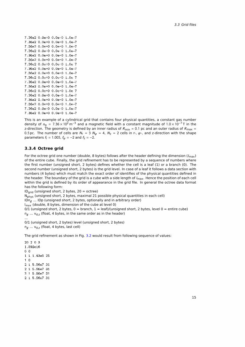
This is an example of a cylindrical grid that contains four physical quantities, a constant gas numberdensity of ng = 7.36 × 10² m−3 and a magnetic field with a constant magnitude of 1.0 × 10⁻⁷ T in thez-direction. The geometry is defined by an inner radius of Rmin = 0.1 pc and an outer radius of Rmax =0.5pc. The number of cells are Nr = 3 Nϕ = 4, Nz = 2 cells in r-, ϕ-, and z-direction with the shapeparameters fr = 1.005, fϕ = −2 and fz = −2.
3.3.4 Octree grid
For the octree grid one number (double, 8 bytes) follows after the header defining the dimension (lmax)of the entire cube. Finally, the grid refinement has to be represented by a sequence of numbers wherethe first number (unsigned short, 2 bytes) defines whether the cell is a leaf (1) or a branch (0). Thesecond number (unsigned short, 2 bytes) is the grid level. In case of a leaf it follows a data section withnumbers (4 bytes) which must match the exact order of identifies of the physical quantities defined inthe header. The boundary of the grid is a cube with a side length of lmax. Hence the position of each cellwithin the grid is defined by its order of appearance in the grid file. In general the octree data formathas the following form:IDgrid (unsigned short, 2 bytes, 20 = octree)Nphys (unsigned short, 2 bytes, maximal 21 possible physical quantities in each cell)IDng ... IDp (unsigned short, 2 bytes, optionally and in arbitrary order)lmax (double, 8 bytes, dimension of the cube at level 0)0/1 (unsigned short, 2 bytes, 0 = branch, 1 = leaf)/(unsigned short, 2 bytes, level 0 = entire cube)ng ... vd,z (float, 4 bytes, in the same order as in the header)...0/1 (unsigned short, 2 bytes) level (unsigned short, 2 bytes)ng ... vd,z (float, 4 bytes, last cell)
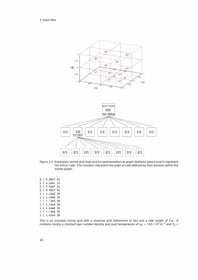
The grid refinement as shown in Fig. 3.2 would result from following sequence of values:
20 2 0 3
1.892e16
0 0
1 1 1.43e5 25
1 0
2 1 5.56e7 31
2 1 5.56e7 31
2 1 5.56e7 31
2 1 5.56e7 31
15
3 Input files
-1-0.5
0 0.5
1 -1
-0.5
0
0.5
1
-1
-0.5
0
0.5
1
z [ly]
1
2 3
4 5
6 7
8 9
10
11
12
13
14
15
x [ly]
y [ly]
z [ly]
leaf / level
1/0
0/0no data
1/1 1/1 1/1 1/1 1/1 1/1 1/1
2/1
no data
2/1 2/1 2/1 2/1 2/1 2/1 2/1
Figure 3.2: Exemplary octree grid (top) and its representation as graph (bottom) where level 0 representthe entire cube. The numbers represent the order of cells defined by their position within theoctree graph.
2 1 5.56e7 31
2 1 5.56e7 31
2 1 5.56e7 31
2 1 5.56e7 31
1 1 1.43e5 25
1 1 1.43e5 25
1 1 1.43e5 25
1 1 1.43e5 25
1 1 1.43e5 25
1 1 1.43e5 25
1 1 1.43e5 25
This is an example octree grid with a maximal grid refinement of two and a side length of 2 ly. Itcontains mostly a constant gas number density and dust temperature of ng = 1.43 × 10⁵ m−3 and Tg =
16
3.3 Grid files
25K, respectively, with a level one refinement. A smaller region has a level two refinement with ng =
5.56 × 10⁷ m−3 and Tg = 31K.
3.3.5 Voronoi grid
−1
−0.5
0
0.5
1 −1
−0.5
0
0.5
1−1
−0.5
0
0.5
1
z[1016 m]
4
7
2
6
1
3
5
x[1016 m] y[1016 m]
z[1016 m]
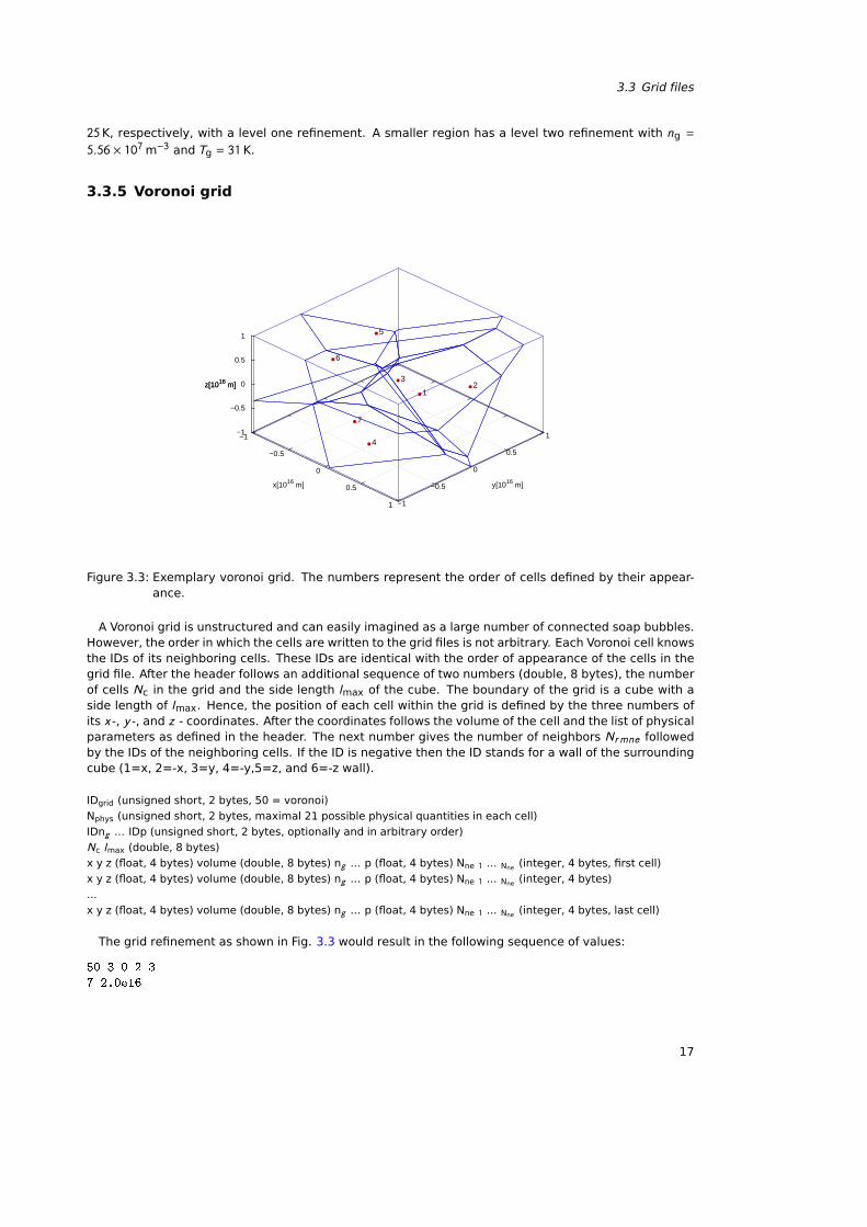
Figure 3.3: Exemplary voronoi grid. The numbers represent the order of cells defined by their appear-ance.
A Voronoi grid is unstructured and can easily imagined as a large number of connected soap bubbles.However, the order in which the cells are written to the grid files is not arbitrary. Each Voronoi cell knowsthe IDs of its neighboring cells. These IDs are identical with the order of appearance of the cells in thegrid file. After the header follows an additional sequence of two numbers (double, 8 bytes), the numberof cells Nc in the grid and the side length lmax of the cube. The boundary of the grid is a cube with aside length of lmax. Hence, the position of each cell within the grid is defined by the three numbers ofits x -, y -, and z - coordinates. After the coordinates follows the volume of the cell and the list of physicalparameters as defined in the header. The next number gives the number of neighbors Nrmne followedby the IDs of the neighboring cells. If the ID is negative then the ID stands for a wall of the surroundingcube (1=x, 2=-x, 3=y, 4=-y,5=z, and 6=-z wall).
IDgrid (unsigned short, 2 bytes, 50 = voronoi)
Nphys (unsigned short, 2 bytes, maximal 21 possible physical quantities in each cell)
IDng ... IDp (unsigned short, 2 bytes, optionally and in arbitrary order)
Nc lmax (double, 8 bytes)
x y z (float, 4 bytes) volume (double, 8 bytes) ng ... p (float, 4 bytes) Nne 1 ... Nne (integer, 4 bytes, first cell)
x y z (float, 4 bytes) volume (double, 8 bytes) ng ... p (float, 4 bytes) Nne 1 ... Nne (integer, 4 bytes)
...
x y z (float, 4 bytes) volume (double, 8 bytes) ng ... p (float, 4 bytes) Nne 1 ... Nne (integer, 4 bytes, last cell)
The grid refinement as shown in Fig. 3.3 would result in the following sequence of values:
50 3 0 2 3
7 2.0e16
17
3 Input files
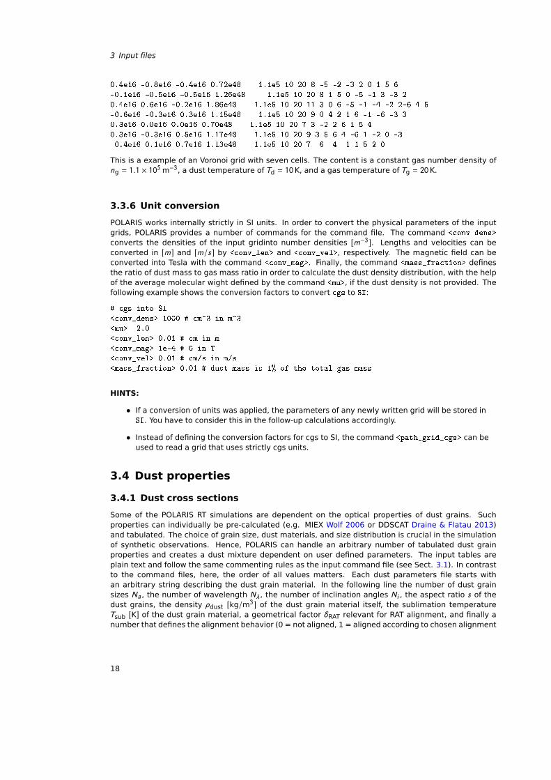
0.4e16 -0.8e16 -0.4e16 0.72e48 1.1e5 10 20 8 -5 -2 -3 2 0 1 5 6
-0.1e16 -0.5e16 -0.5e16 1.26e48 1.1e5 10 20 8 1 5 0 -5 -1 3 -3 2
0.4e16 0.6e16 -0.2e16 1.86e48 1.1e5 10 20 11 3 0 6 -5 -1 -4 -2 2-6 4 5
-0.6e16 -0.3e16 0.3e16 1.15e48 1.1e5 10 20 9 0 4 2 1 6 -1 -6 -3 3
0.3e16 0.0e16 0.0e16 0.70e48 1.1e5 10 20 7 3 -2 2 6 1 5 4
0.3e16 -0.3e16 0.5e16 1.17e48 1.1e5 10 20 9 3 5 6 4 -6 1 -2 0 -3
-0.4e16 0.1e16 0.7e16 1.13e48 1.1e5 10 20 7 -6 -4 -1 1 5 2 0
This is a example of an Voronoi grid with seven cells. The content is a constant gas number density ofng = 1.1 × 10⁵ m−3, a dust temperature of Td = 10K, and a gas temperature of Tg = 20K.
3.3.6 Unit conversion
POLARIS works internally strictly in SI units. In order to convert the physical parameters of the inputgrids, POLARIS provides a number of commands for the command file. The command <conv_dens>
converts the densities of the input gridinto number densities [m−3]. Lengths and velocities can beconverted in [m] and [m/s] by <conv_len> and <conv_vel>, respectively. The magnetic field can beconverted into Tesla with the command <conv_mag>. Finally, the command <mass_fraction> definesthe ratio of dust mass to gas mass ratio in order to calculate the dust density distribution, with the helpof the average molecular wight defined by the command <mu>, if the dust density is not provided. Thefollowing example shows the conversion factors to convert cgs to SI:
# cgs into SI
<conv_dens> 1000 # cm^3 in m^3
<mu> 2.0
<conv_len> 0.01 # cm in m
<conv_mag> 1e-4 # G in T
<conv_vel> 0.01 # cm/s in m/s
<mass_fraction> 0.01 # dust mass is 1% of the total gas mass
HINTS:
• If a conversion of units was applied, the parameters of any newly written grid will be stored inSI. You have to consider this in the follow-up calculations accordingly.
• Instead of defining the conversion factors for cgs to SI, the command <path_grid_cgs> can beused to read a grid that uses strictly cgs units.
3.4 Dust properties
3.4.1 Dust cross sections
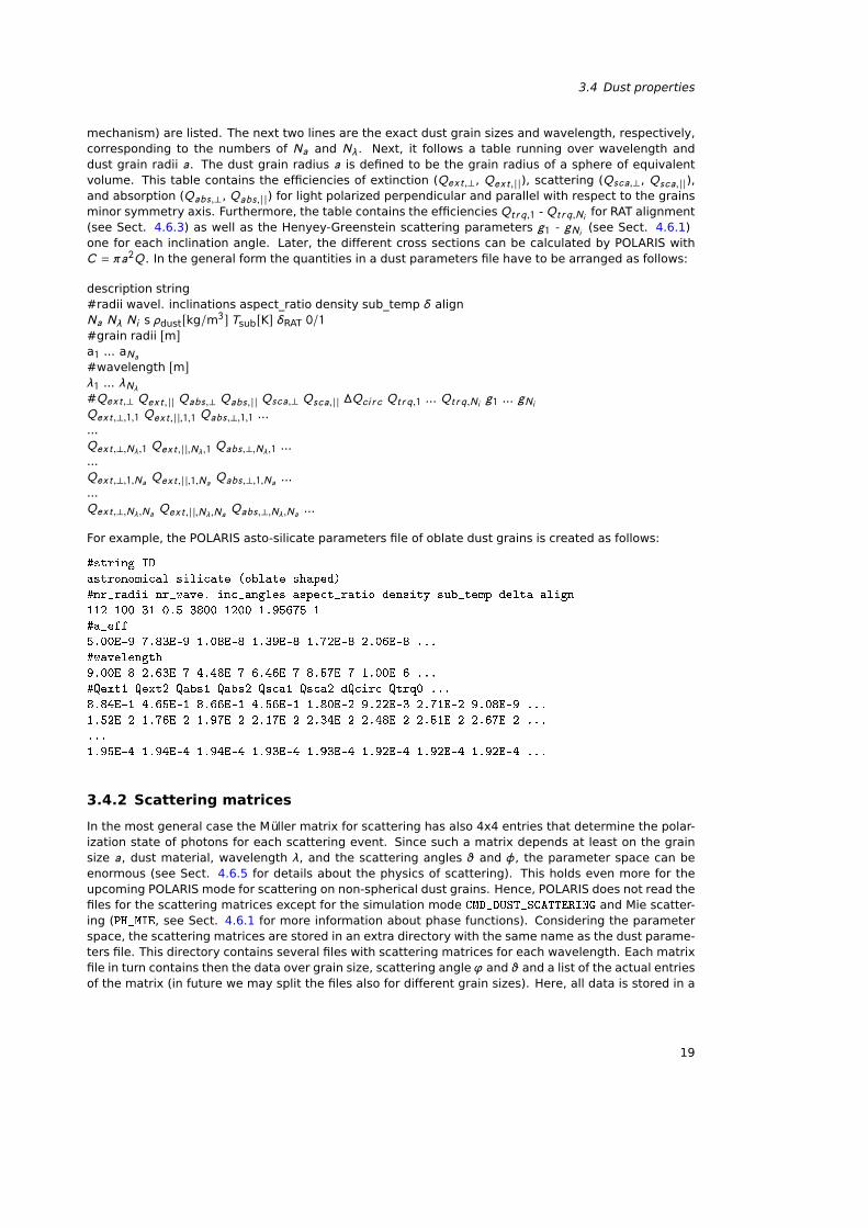
Some of the POLARIS RT simulations are dependent on the optical properties of dust grains. Suchproperties can individually be pre-calculated (e.g. MIEX Wolf 2006 or DDSCAT Draine & Flatau 2013)and tabulated. The choice of grain size, dust materials, and size distribution is crucial in the simulationof synthetic observations. Hence, POLARIS can handle an arbitrary number of tabulated dust grainproperties and creates a dust mixture dependent on user defined parameters. The input tables areplain text and follow the same commenting rules as the input command file (see Sect. 3.1). In contrastto the command files, here, the order of all values matters. Each dust parameters file starts withan arbitrary string describing the dust grain material. In the following line the number of dust grainsizes Na , the number of wavelength Nλ , the number of inclination angles Ni , the aspect ratio s of thedust grains, the density ρdust [kg/m3] of the dust grain material itself, the sublimation temperatureTsub [K] of the dust grain material, a geometrical factor δRAT relevant for RAT alignment, and finally anumber that defines the alignment behavior (0 = not aligned, 1 = aligned according to chosen alignment
18
3.4 Dust properties
mechanism) are listed. The next two lines are the exact dust grain sizes and wavelength, respectively,corresponding to the numbers of Na and Nλ . Next, it follows a table running over wavelength anddust grain radii a. The dust grain radius a is defined to be the grain radius of a sphere of equivalentvolume. This table contains the efficiencies of extinction (Qext ,⊥, Qext , | |), scattering (Qsca,⊥, Qsca, | |),and absorption (Qabs,⊥, Qabs, | |) for light polarized perpendicular and parallel with respect to the grainsminor symmetry axis. Furthermore, the table contains the efficiencies Qt r q ,1 - Qt r q ,N i for RAT alignment(see Sect. 4.6.3) as well as the Henyey-Greenstein scattering parameters g1 - gN i (see Sect. 4.6.1)one for each inclination angle. Later, the different cross sections can be calculated by POLARIS withC = πa2Q . In the general form the quantities in a dust parameters file have to be arranged as follows:
description string#radii wavel. inclinations aspect_ratio density sub_temp δ alignNa Nλ Ni s ρdust[kg/m3] Tsub[K] δRAT 0/1#grain radii [m]a1 ... aNa#wavelength [m]λ1 ... λNλ#Qext ,⊥ Qext , | | Qabs,⊥ Qabs, | | Qsca,⊥ Qsca, | | ∆Qci r c Qt r q ,1 ... Qt r q ,N i g1 ... gN iQext ,⊥,1,1 Qext , | |,1,1 Qabs,⊥,1,1 ......Qext ,⊥,Nλ ,1 Qext , | |,Nλ ,1 Qabs,⊥,Nλ ,1 ......Qext ,⊥,1,Na Qext , | |,1,Na Qabs,⊥,1,Na ......Qext ,⊥,Nλ ,Na Qext , | |,Nλ ,Na Qabs,⊥,Nλ ,Na ...
For example, the POLARIS asto-silicate parameters file of oblate dust grains is created as follows:
#string ID
astronomical silicate (oblate shaped)
#nr_radii nr_wave. inc_angles aspect_ratio density sub_temp delta align
112 100 31 0.5 3800 1200 1.95675 1
#a_eff
5.00E-9 7.83E-9 1.08E-8 1.39E-8 1.72E-8 2.06E-8 ...
#wavelength
9.00E-8 2.63E-7 4.48E-7 6.46E-7 8.57E-7 1.00E-6 ...
#Qext1 Qext2 Qabs1 Qabs2 Qsca1 Qsca2 dQcirc Qtrq0 ...
8.84E-1 4.65E-1 8.66E-1 4.56E-1 1.80E-2 9.22E-3 2.71E-2 9.08E-9 ...
1.52E-2 1.76E-2 1.97E-2 2.17E-2 2.34E-2 2.48E-2 2.51E-2 2.67E-2 ...
...
1.95E-4 1.94E-4 1.94E-4 1.93E-4 1.93E-4 1.92E-4 1.92E-4 1.92E-4 ...
3.4.2 Scattering matrices
In the most general case the Müller matrix for scattering has also 4x4 entries that determine the polar-ization state of photons for each scattering event. Since such a matrix depends at least on the grainsize a, dust material, wavelength λ, and the scattering angles ϑ and φ, the parameter space can beenormous (see Sect. 4.6.5 for details about the physics of scattering). This holds even more for theupcoming POLARIS mode for scattering on non-spherical dust grains. Hence, POLARIS does not read thefiles for the scattering matrices except for the simulation mode CMD_DUST_SCATTERING and Mie scatter-ing (PH_MIE, see Sect. 4.6.1 for more information about phase functions). Considering the parameterspace, the scattering matrices are stored in an extra directory with the same name as the dust parame-ters file. This directory contains several files with scattering matrices for each wavelength. Each matrixfile in turn contains then the data over grain size, scattering angle ϕ and ϑ and a list of the actual entriesof the matrix (in future we may split the files also for different grain sizes). Here, all data is stored in a
19
3 Input files
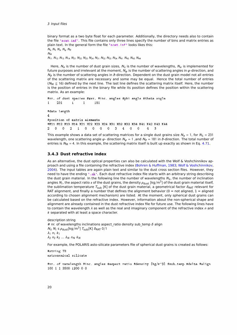
binary format as a two byte float for each parameter. Additionally, the directory needs also to containthe file 'scat.inf'. This file contains only three lines specify the number of bins and matrix entries asplain text. In the general form the file 'scat.inf' looks likes this:Na Nλ Nα Nϕ NϑNM
N11 N12 N13 N14 N21 N22 N23 N24 N31 N32 N33 N34 N41 N42 N43 N44
Here, Na is the number of dust grain sizes, Nλ is the number of wavelengths, Nα is implemented forfuture purposes and irrelevant at the moment, Nϕ is the number of scattering angles in ϕ-direction, andNϑ is the number of scattering angles in ϑ-direction. Dependent on the dust grain model not all entriesof the scattering matrix are necessary and some may be equal. Hence the total number of entries(NM 5 16) defined by the next line. The last line defines the scattering matrix itself. Here, the numberis the position of entries in the binary file while its position defines the position within the scatteringmatrix. As an example:
#nr. of dust species #wav. #inc. angles #phi angle #theta angle
1 231 1 1 181
#data length
4
#position of matrix elements
#M11 M12 M13 M14 M21 M22 M23 M24 M31 M32 M33 M34 M41 M42 M43 M44
2 0 0 2 1 0 0 0 0 3 4 0 0 -4 3
This example shows a data set of scattering matrices for a single dust grains size Na = 1, for Nλ = 231wavelength, one scattering angle ϕ- direction Nϕ = 1 ,and Nϑ = 181 in ϑ-direction. The total number ofentries is NM = 4. In this example, the scattering matrix itself is built up exactly as shown in Eq. 4.71.
3.4.3 Dust refractive index
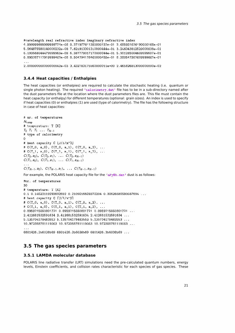
As an alternative, the dust optical properties can also be calculated with the Wolf & Voshchinnikov ap-proach and using a file containing the refractive index (Bohren & Huffman, 1983; Wolf & Voshchinnikov,2004). The input tables are again plain text and similar to the dust cross section files. However, theyneed to have the ending '.nk'. Each dust refractive index file starts with an arbitrary string describingthe dust grain material. In the following line the number of wavelengths Nλ , the number of inclinationangles Ni , the aspect ratio s of the dust grains, the density ρdust [kg/m3] of the dust grain material itself,the sublimation temperature Tsub [K] of the dust grain material, a geometrical factor δRAT relevant forRAT alignment, and finally a number that defines the alignment behavior (0 = not aligned, 1 = alignedaccording to chosen alignment mechanism) are listed. At the moment, only spherical dust grains canbe calculated based on the refractive index. However, information about the non-spherical shape andalignment are already contained in the dust refractive index file for future use. The following lines haveto contain the wavelength λ as well as the real and imaginary component of the refractive index n andk separated with at least a space character.
description string# nr. of wavelengths inclinations aspect_ratio density sub_temp δ alignNλ Ni s ρdust[kg/m3] Tsub[K] δRAT 0/1λ1 n1 k1λ2 n2 k2 ... λN nN kN
For example, the POLARIS asto-silicate parameters file of spherical dust grains is created as follows:
#string ID
astronomical silicate
#nr. of wavelength #inc. angles #aspect ratio #density [kg/m^3] #sub.temp #delta #align
100 1 1 3500 1200 0 0
20
3.5 The gas species parameters
#wavelength real refractive index imaginary refractive index
4.999999999999999774e-08 8.271977641350000132e-01 2.685931626490000168e-01
5.564875580140000232e-08 7.621913301310000444e-01 3.246343812520000038e-01
6.193568044479999963e-08 6.387779917170000044e-01 5.901285004609999607e-01
6.893287112919999462e-08 8.504294128460000435e-01 8.380542302629999662e-01
...
2.000000000000000042e-03 3.432783175560000011e+00 2.465826813000000090e-02
3.4.4 Heat capacities / Enthalpies
The heat capacities (or enthalpies) are required to calculate the stochastic heating (i.e. quantum orsingle photon heating). The required 'calorimetry.dat' file has to be in a sub-directory named afterthe dust parameters file at the location where the dust parameters files are. This file must contain theheat capacity (or enthalpy) for different temperatures (optional: grain sizes). An index is used to specifyif heat capacities (0) or enthalpies (1) are used (type of calorimetry). The file has the following structurein case of heat capacities:
# nr. of temperatures
Ntemp
# temperature: T [K]
T0 T1 T1 ... TN−1# type of calorimetry
0
# heat capacity C [J/K/m^3]
# C(T_0, a_0), C(T_0, a_1), C(T_0, a_2), ...
# C(T_1, a_0), C(T_1, a_1), C(T_1, a_2), ...
C (T0, a0), C (T0, a1), ... C (T0, aN−1)C (T1, a0), C (T1, a1), ... C (T1, aN−1)...
C (TN−1, a0), C (TN−1, a1), ... C (TN−1, aN−1)For example, the POLARIS heat capacity file for the 'aPyM5.dat' dust is as follows:
#nr. of temperatures
30
# temperature: T [K]
0.1 0.14522119293692692 0.2109016609370204 0.30626685580037694 ...
# heat capacity C [J/K/m^3]
# C(T_0, a_0), C(T_0, a_1), C(T_0, a_2), ...
# C(T_1, a_0), C(T_1, a_1), C(T_1, a_2), ...
0.8959215850801721 0.8959215850801721 0.8959215850801721 ...
2.412681532591634 2.412681532591634 2.412681532591634 ...
5.135704178483553 5.135704178483553 5.135704178483553 ...
10.972358781119063 10.972358781119063 10.972358781119063 ...
...
6801426.356038569 6801426.356038569 6801426.356038569 ...
3.5 The gas species parameters
3.5.1 LAMDA molecular database
POLARIS line radiative transfer (LRT) simulations need the pre-calculated quantum numbers, energylevels, Einstein coefficients, and collision rates characteristic for each species of gas species. These
21
3 Input files
molecular parameters files are publicly available at the LAMDA (Leiden Atomic and Molecular Database)website: http://home.strw.leidenuniv.nl/~moldata/. The provided LAMDA file format is fully sup-ported by POLARIS without any intermediate conversion step. Lines beginning with a ! are commentsand will be ignored by the POLARIS command parser.
Since the LAMDA database is an external source, we just provide a short description of the file formatin this manual as far as it is relevant for the POLARIS code. For additional information see http://
home.strw.leidenuniv.nl/~moldata/. The first parameter in a LAMDA file is a string with the name ofthe gas species. The next number is the molecular weight followed by the numbers of pre-calculatedenergy levels. In the following table the energy levels, the energy on each level itself, and the quantumnumber of each level are listed. The number of pre-calulated transitions is in the line followed by asecond table. This table provides the an unique ID for each transition the number of energy levelsbetween which the transition occurs, the Einstein A coefficient , as well as the characteristic frequencyof the transition. The unique transition ID in this table is relevant for the POLARIS command files (see3.1) and the Zeeman parameters file (see 3.5.2) in order to select the desired transitions. The nextfour lines define the number of considered collision partners to calculate the collisional excitation, astring identifying the collision partner and the reference of this data, the number of collision transitions,and finally the number of collision temperatures. The tables are at the end of the file and provide thephysical parameters for all of permutations of collision partners, transitions and collision temperatures.
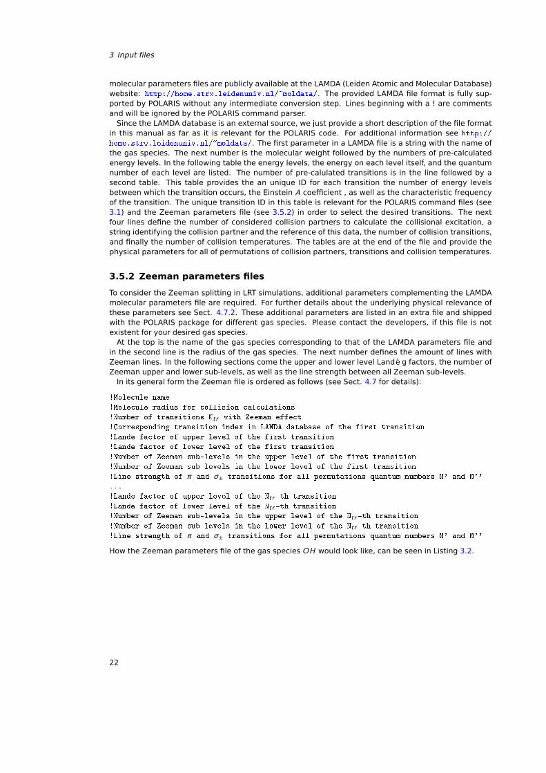
3.5.2 Zeeman parameters files
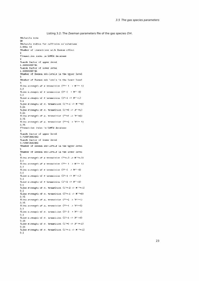
To consider the Zeeman splitting in LRT simulations, additional parameters complementing the LAMDAmolecular parameters file are required. For further details about the underlying physical relevance ofthese parameters see Sect. 4.7.2. These additional parameters are listed in an extra file and shippedwith the POLARIS package for different gas species. Please contact the developers, if this file is notexistent for your desired gas species.
At the top is the name of the gas species corresponding to that of the LAMDA parameters file andin the second line is the radius of the gas species. The next number defines the amount of lines withZeeman lines. In the following sections come the upper and lower level Landè g factors, the number ofZeeman upper and lower sub-levels, as well as the line strength between all Zeeman sub-levels.
In its general form the Zeeman file is ordered as follows (see Sect. 4.7 for details):
!Molecule name
!Molecule radius for collision calculations
!Number of transitions Nt r with Zeeman effect
!Corresponding transition index in LAMDA database of the first transition
!Lande factor of upper level of the first transition
!Lande factor of lower level of the first transition
!Number of Zeeman sub-levels in the upper level of the first transition
!Number of Zeeman sub-levels in the lower level of the first transition
!Line strength of π and σ± transitions for all permutations quantum numbers M' and M''
...
!Lande factor of upper level of the Nt r -th transition
!Lande factor of lower level of the Nt r -th transition
!Number of Zeeman sub-levels in the upper level of the Nt r -th transition
!Number of Zeeman sub-levels in the lower level of the Nt r -th transition
!Line strength of π and σ± transitions for all permutations quantum numbers M' and M''
How the Zeeman parameters file of the gas species OH would look like, can be seen in Listing 3.2.
22
3.5 The gas species parameters
Listing 3.2: The Zeeman parameters file of the gas species OH .
!Molecule name
OH
!Molecule radius for collision calculations
0.958e-10
!Number of transitions with Zeeman effect
2
!Transition index in LAMDA database
2
!Lande factor of upper level
1.16828926744
!Lande factor of lower level
1.16828926744
!Number of Zeeman sub-levels in the upper level
3
!Number of Zeeman sub-levels in the lower level
3
!Line strength of π transition (M'=-1 -> M''=-1)
0.5
!Line strength of π transition (M'=0 -> M''=0)
0.0
!Line strength of π transition (M'=1 -> M''=1)
0.5
!Line strength of σ+ transition (M'=-1 -> M''=0)
0.25
!Line strength of σ+ transition (M'=0 -> M''=1)
0.25
!Line strength of σ− transition (M'=1 -> M''=0)
0.25
!Line strength of σ− transition (M'=0 -> M''=-1)
0.25
!Transition index in LAMDA database
3
!Lande factor of upper level
0.700973560462
!Lande factor of lower level
0.700973560462
!Number of Zeeman sub-levels in the upper level
5
!Number of Zeeman sub-levels in the lower level
5
!Line strength of π transition (M'=-2 -> M''=-2)
0.4
!Line strength of π transition (M'=-1 -> M''=-1)
0.1
!Line strength of π transition (M'=0 -> M''=0)
0.0
!Line strength of π transition (M'=1 -> M''=1)
0.1
!Line strength of π transition (M'=2 -> M''=2)
0.4
!Line strength of σ+ transition (M'=-2 -> M''=-1)
0.1
!Line strength of σ+ transition (M'=-1 -> M''=0)
0.15
!Line strength of σ+ transition (M'=0 -> M''=1)
0.15
!Line strength of σ+ transition (M'=1 -> M''=2)
0.1
!Line strength of σ− transition (M'=2 -> M''=1)
0.1
!Line strength of σ− transition (M'=1 -> M''=0)
0.15
!Line strength of σ− transition (M'=0 -> M''=-1)
0.15
!Line strength of σ− transition (M'=-1 -> M''=-2)
0.1
23
3 Input files
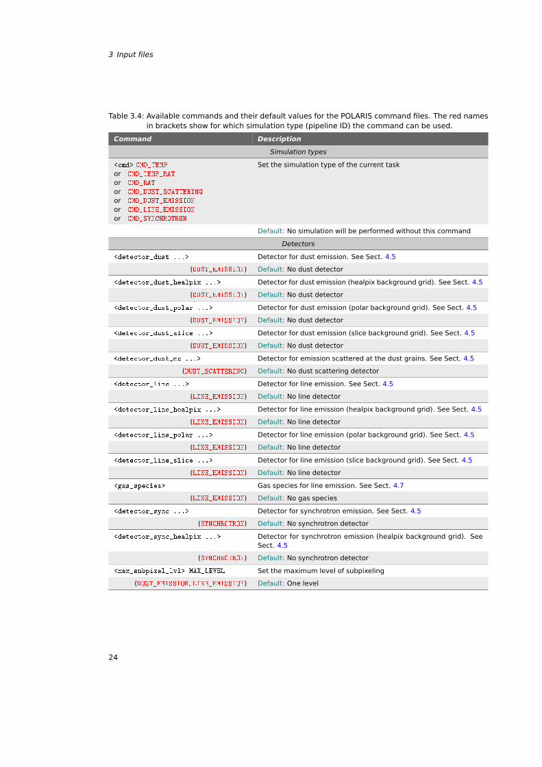
Table 3.4: Available commands and their default values for the POLARIS command files. The red namesin brackets show for which simulation type (pipeline ID) the command can be used.
Command Description
Simulation types
<cmd> CMD_TEMP
or CMD_TEMP_RAT
or CMD_RAT
or CMD_DUST_SCATTERING
or CMD_DUST_EMISSION
or CMD_LINE_EMISSION
or CMD_SYNCHROTRON
Set the simulation type of the current task
Default: No simulation will be performed without this command
Detectors
<detector_dust ...> Detector for dust emission. See Sect. 4.5
(DUST_EMISSION) Default: No dust detector
<detector_dust_healpix ...> Detector for dust emission (healpix background grid). See Sect. 4.5
(DUST_EMISSION) Default: No dust detector
<detector_dust_polar ...> Detector for dust emission (polar background grid). See Sect. 4.5
(DUST_EMISSION) Default: No dust detector
<detector_dust_slice ...> Detector for dust emission (slice background grid). See Sect. 4.5
(DUST_EMISSION) Default: No dust detector
<detector_dust_mc ...> Detector for emission scattered at the dust grains. See Sect. 4.5
(DUST_SCATTERING) Default: No dust scattering detector
<detector_line ...> Detector for line emission. See Sect. 4.5
(LINE_EMISSION) Default: No line detector
<detector_line_healpix ...> Detector for line emission (healpix background grid). See Sect. 4.5
(LINE_EMISSION) Default: No line detector
<detector_line_polar ...> Detector for line emission (polar background grid). See Sect. 4.5
(LINE_EMISSION) Default: No line detector
<detector_line_slice ...> Detector for line emission (slice background grid). See Sect. 4.5
(LINE_EMISSION) Default: No line detector
<gas_species> Gas species for line emission. See Sect. 4.7
(LINE_EMISSION) Default: No gas species
<detector_sync ...> Detector for synchrotron emission. See Sect. 4.5
(SYNCHROTRON) Default: No synchrotron detector
<detector_sync_healpix ...> Detector for synchrotron emission (healpix background grid). SeeSect. 4.5
(SYNCHROTRON) Default: No synchrotron detector
<max_subpixel_lvl> MAX_LEVEL Set the maximum level of subpixeling
(DUST_EMISSION, LINE_EMISSION) Default: One level
24
3.5 The gas species parameters
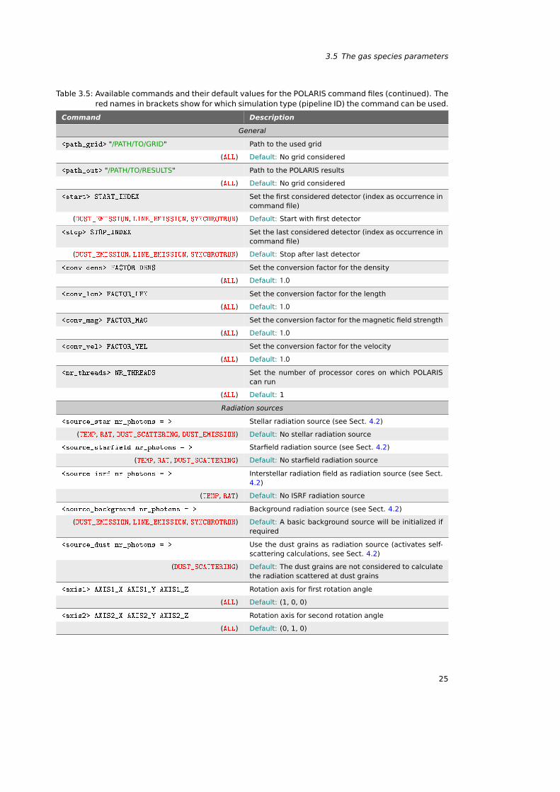
Table 3.5: Available commands and their default values for the POLARIS command files (continued). Thered names in brackets show for which simulation type (pipeline ID) the command can be used.
Command Description
General
<path_grid> "/PATH/TO/GRID" Path to the used grid
(ALL) Default: No grid considered
<path_out> "/PATH/TO/RESULTS" Path to the POLARIS results
(ALL) Default: No grid considered
<start> START_INDEX Set the first considered detector (index as occurrence incommand file)
(DUST_EMISSION, LINE_EMISSION, SYNCHROTRON) Default: Start with first detector
<stop> STOP_INDEX Set the last considered detector (index as occurrence incommand file)
(DUST_EMISSION, LINE_EMISSION, SYNCHROTRON) Default: Stop after last detector
<conv_dens> FACTOR_DENS Set the conversion factor for the density
(ALL) Default: 1.0
<conv_len> FACTOR_LEN Set the conversion factor for the length
(ALL) Default: 1.0
<conv_mag> FACTOR_MAG Set the conversion factor for the magnetic field strength
(ALL) Default: 1.0
<conv_vel> FACTOR_VEL Set the conversion factor for the velocity
(ALL) Default: 1.0
<nr_threads> NR_THREADS Set the number of processor cores on which POLARIScan run
(ALL) Default: 1
Radiation sources
<source_star nr_photons = > Stellar radiation source (see Sect. 4.2)
(TEMP, RAT, DUST_SCATTERING, DUST_EMISSION) Default: No stellar radiation source
<source_starfield nr_photons = > Starfield radiation source (see Sect. 4.2)
(TEMP, RAT, DUST_SCATTERING) Default: No starfield radiation source
<source_isrf nr_photons = > Interstellar radiation field as radiation source (see Sect.4.2)
(TEMP, RAT) Default: No ISRF radiation source
<source_background nr_photons = > Background radiation source (see Sect. 4.2)
(DUST_EMISSION, LINE_EMISSION, SYNCHROTRON) Default: A basic background source will be initialized ifrequired
<source_dust nr_photons = > Use the dust grains as radiation source (activates self-scattering calculations, see Sect. 4.2)
(DUST_SCATTERING) Default: The dust grains are not considered to calculatethe radiation scattered at dust grains
<axis1> AXIS1_X AXIS1_Y AXIS1_Z Rotation axis for first rotation angle
(ALL) Default: (1, 0, 0)
<axis2> AXIS2_X AXIS2_Y AXIS2_Z Rotation axis for second rotation angle
(ALL) Default: (0, 1, 0)
25
3 Input files
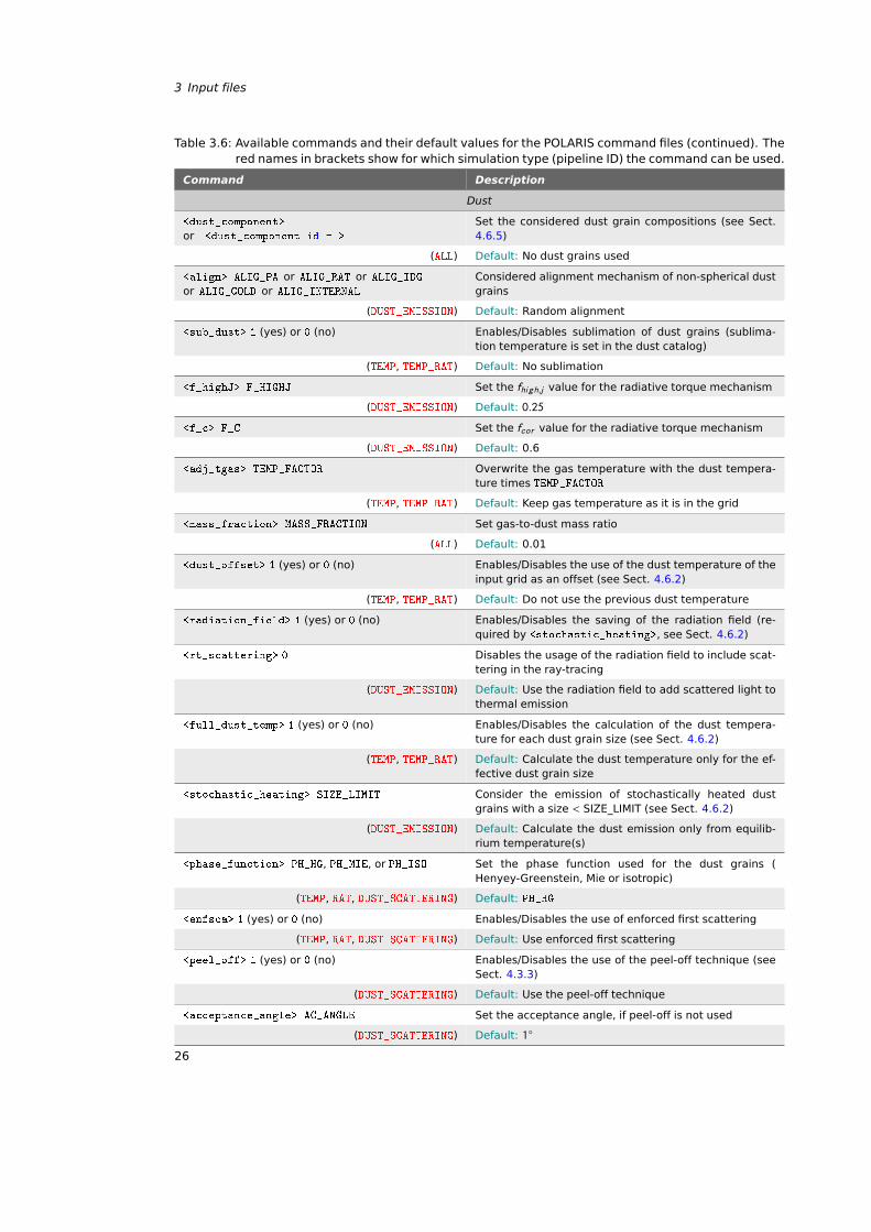
Table 3.6: Available commands and their default values for the POLARIS command files (continued). Thered names in brackets show for which simulation type (pipeline ID) the command can be used.
Command Description
Dust
<dust_component>
or <dust_component id = >
Set the considered dust grain compositions (see Sect.4.6.5)
(ALL) Default: No dust grains used
<align> ALIG_PA or ALIG_RAT or ALIG_IDG
or ALIG_GOLD or ALIG_INTERNAL
Considered alignment mechanism of non-spherical dustgrains
(DUST_EMISSION) Default: Random alignment
<sub_dust> 1 (yes) or 0 (no) Enables/Disables sublimation of dust grains (sublima-tion temperature is set in the dust catalog)
(TEMP, TEMP_RAT) Default: No sublimation
<f_highJ> F_HIGHJ Set the fhi gh,j value for the radiative torque mechanism
(DUST_EMISSION) Default: 0.25
<f_c> F_C Set the fcor value for the radiative torque mechanism
(DUST_EMISSION) Default: 0.6
<adj_tgas> TEMP_FACTOR Overwrite the gas temperature with the dust tempera-ture times TEMP_FACTOR
(TEMP, TEMP_RAT) Default: Keep gas temperature as it is in the grid
<mass_fraction> MASS_FRACTION Set gas-to-dust mass ratio
(ALL) Default: 0.01
<dust_offset> 1 (yes) or 0 (no) Enables/Disables the use of the dust temperature of theinput grid as an offset (see Sect. 4.6.2)
(TEMP, TEMP_RAT) Default: Do not use the previous dust temperature
<radiation_field> 1 (yes) or 0 (no) Enables/Disables the saving of the radiation field (re-quired by <stochastic_heating>, see Sect. 4.6.2)
<rt_scattering> 0 Disables the usage of the radiation field to include scat-tering in the ray-tracing
(DUST_EMISSION) Default: Use the radiation field to add scattered light tothermal emission
<full_dust_temp> 1 (yes) or 0 (no) Enables/Disables the calculation of the dust tempera-ture for each dust grain size (see Sect. 4.6.2)
(TEMP, TEMP_RAT) Default: Calculate the dust temperature only for the ef-fective dust grain size
<stochastic_heating> SIZE_LIMIT Consider the emission of stochastically heated dustgrains with a size < SIZE_LIMIT (see Sect. 4.6.2)
(DUST_EMISSION) Default: Calculate the dust emission only from equilib-rium temperature(s)
<phase_function> PH_HG, PH_MIE, or PH_ISO Set the phase function used for the dust grains (Henyey-Greenstein, Mie or isotropic)
(TEMP, RAT, DUST_SCATTERING) Default: PH_HG
<enfsca> 1 (yes) or 0 (no) Enables/Disables the use of enforced first scattering
(TEMP, RAT, DUST_SCATTERING) Default: Use enforced first scattering
<peel_off> 1 (yes) or 0 (no) Enables/Disables the use of the peel-off technique (seeSect. 4.3.3)
(DUST_SCATTERING) Default: Use the peel-off technique
<acceptance_angle> AC_ANGLE Set the acceptance angle, if peel-off is not used
(DUST_SCATTERING) Default: 1
26
3.5 The gas species parameters
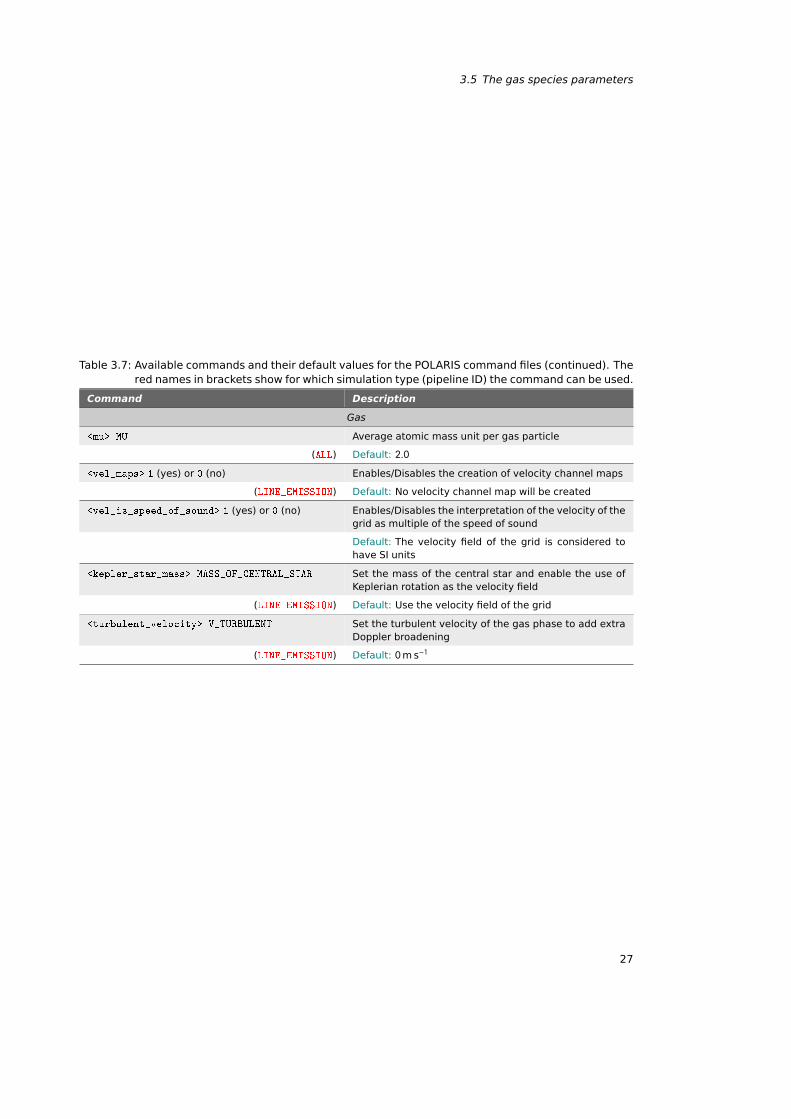
Table 3.7: Available commands and their default values for the POLARIS command files (continued). Thered names in brackets show for which simulation type (pipeline ID) the command can be used.
Command Description
Gas
<mu> MU Average atomic mass unit per gas particle
(ALL) Default: 2.0
<vel_maps> 1 (yes) or 0 (no) Enables/Disables the creation of velocity channel maps
(LINE_EMISSION) Default: No velocity channel map will be created
<vel_is_speed_of_sound> 1 (yes) or 0 (no) Enables/Disables the interpretation of the velocity of thegrid as multiple of the speed of sound
Default: The velocity field of the grid is considered tohave SI units
<kepler_star_mass> MASS_OF_CENTRAL_STAR Set the mass of the central star and enable the use ofKeplerian rotation as the velocity field
(LINE_EMISSION) Default: Use the velocity field of the grid
<turbulent_velocity> V_TURBULENT Set the turbulent velocity of the gas phase to add extraDoppler broadening
(LINE_EMISSION) Default: 0m s−1
27
3 Input files
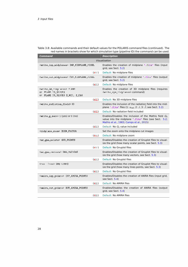
Table 3.8: Available commands and their default values for the POLARIS command files (continued). Thered names in brackets show for which simulation type (pipeline ID) the command can be used.
Command Description
Visualization
<write_inp_midplanes> INP_MIDPLANE_PIXEL Enables the creation of midplane '.fits' files (inputgrid, see Sect. 5.2)
(ALL) Default: No midplane files
<write_out_midplanes> OUT_MIDPLANE_PIXEL Enables the creation of midplane '.fits' files (outputgrid, see Sect. 5.2)
(ALL) Default: No midplane files
<write_3d_midplanes> PLANE
or PLANE NR_SLICES
or PLANE NR_SLICES Z_MIN, Z_MAX
Enables the creation of 3D midplane files (requires<write_xyz_midplanes> command)
(ALL) Default: No 3D midplane files
<write_radiation_field> ID Enables the inclusion of the radiation field into the mid-plane '.fits' files (1: urad, 2: J , 3: ®J ; see Sect. 5.2)
(ALL) Default: No radiation field included
<write_g_zero> 1 (yes) or 0 (no) Enables/Disables the inclusion of the Mathis field G0value into the midplane '.fits' files (see Sect. 5.2;Mathis et al., 1983; Camps et al., 2015)
(ALL) Default: No G0 value included
<midplane_zoom> ZOOM_FACTOR Set the zoom onto the midplane cut images
(ALL) Default: No midplane zoom
<nr_gnu_points> GNU_POINTS Enables/Disables the creation of Gnuplot files to visual-ize the grid (how many scalar points, see Sect. 5.3)
(ALL) Default: No Gnuplot files
<nr_gnu_vectors> GNU_VECTORS Enables/Disables the creation of Gnuplot files to visual-ize the grid (how many vectors, see Sect. 5.3)
(ALL) Default: No Gnuplot files
<max_lines> GNU_LINES Enables/Disables the creation of Gnuplot files to visual-ize the grid (how many lines points, see Sect. 5.3)
(ALL) Default: No Gnuplot files
<amira_inp_points> INP_AMIRA_POINTS Enables/Disables the creation of ANIRA files (input grid,see Sect. 5.4)
(ALL) Default: No AMIRA files
<amira_out_points> OUT_AMIRA_POINTS Enables/Disables the creation of ANIRA files (outputgrid, see Sect. 5.4)
(ALL) Default: No AMIRA files
28
4 POLARIS pipeline
The POLARIS code works in independent distinct simulation modes. The choice of modes depends onthe scientific interest of the user. All modes can be combined into a single command file. In this sectionwe describe the different POLARIS modes and outline the underlying physical principles of dust andmolecular line, and synchrotron RT, respectively, as well as the implemented numerical methods.
4.1 Photon propagation
4.1.1 The Stokes vector
Y
XEX
EYY
X
E45E-45
Y
X
ECW ECCW
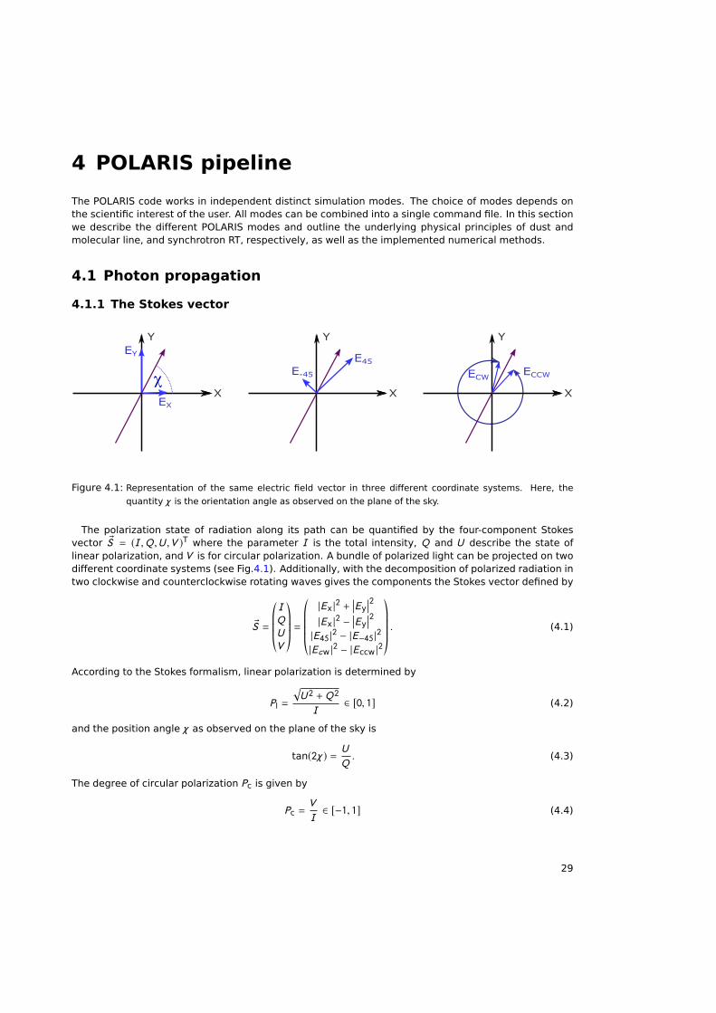
Figure 4.1: Representation of the same electric field vector in three different coordinate systems. Here, the
quantity χ is the orientation angle as observed on the plane of the sky.
The polarization state of radiation along its path can be quantified by the four-component Stokesvector ®S = (I ,Q ,U ,V )T where the parameter I is the total intensity, Q and U describe the state oflinear polarization, andV is for circular polarization. A bundle of polarized light can be projected on twodifferent coordinate systems (see Fig.4.1). Additionally, with the decomposition of polarized radiation intwo clockwise and counterclockwise rotating waves gives the components the Stokes vector defined by
®S =©«IQUV
ª®®®¬ =©«|Ex |2 +
Ey2
|Ex |2 −Ey
2|E45 |2 − |E−45 |2|Ecw |2 − |Eccw |2
ª®®®®¬. (4.1)
According to the Stokes formalism, linear polarization is determined by
Pl =
√U 2 + Q 2
I∈ [0, 1] (4.2)
and the position angle χ as observed on the plane of the sky is
tan(2χ) = U
Q. (4.3)
The degree of circular polarization Pc is given by
Pc =V
I∈ [−1, 1] (4.4)
29
4 POLARIS pipeline
where Pc = 1 stands for circular polarization with the electric field vector rotating counter clockwise andPc = −1 stands a rotation clockwise towards the observer. Additionally, each photon package in POLARISkeeps also track about the optical depth and column density aling its path.
4.1.2 General radiative transfer equation
The POLARIS code solves the RT equation in all four Stokes parameters simultaneously. This problemcan be expressed as
d
d`®S = −R (α)K R−1(α) ®S + ®J (4.5)
Here, R (α) is a rotation matrix, and ®J is the contribution due to emission. The quantity K is the Müllermatrix describing the extinction, absorption, ans scattering, respectively. Both K as well as ®J are de-fined by the characteristic physics of radiation interacting with gas species, free electrons, or dust,respectively. In the most general form the RT problem can be written as
d
d`
©«IQUV
ª®®®¬ = −©«αI αQ αU αVαQ αI κV κUαU −κV αI κQαV −κU −κQ αI
ª®®®¬©«IQUV
ª®®®¬ +©«jIjQjUjV
ª®®®¬ (4.6)
Dependent on the physical problem some of the coefficients can be eliminated by rotating the polarizedradiation from the lab frame into the target frame meaning the frame of the magnetic field or thesymmetry axis of the dust grain, respectively. From the definition of the Stokes vector follows for therotation:
R (α) =©«1 0 0 00 cos(2φ) − sin(2φ) 00 sin(2φ) cos(2φ) 00 0 0 1
ª®®®¬ . (4.7)
Implemented in the POLARIS is the Runge-Kutta Fehlberg (RFK45) solver in order to provide a highaccuracy solution to the RT problem. This method uses an inbuilt step size ` correction to keep theerror within below a threshold εerr by comparing the forth order Runge Kutta approximation
yk+1 = yk +25
216k1 +
1408
2565k3 +
2197
4101k4 −
1
5k5 (4.8)
with the fifth order solution
yk+1 = yk +25
216k1 +
1408
2565k3 +
2197
4101k4 −
1
5k5 (4.9)
Here, the factors are defined byk1 = l f (tk , yk ), (4.10)
k2 = l f (tk +1
4h, yk +
1
4k1), (4.11)
k3 = l f (tk +3
8h, yk +
3
32k1 +
9
32k2), (4.12)
k4 = l f (tk +12
13h, yk +
1932
2197k1 −
7200
2197k2 +
7296
2197k3), (4.13)
k5 = l f (tk + h, yk +439
216k1 + 8k2 −
3680
513k3 −
854
4104k4), (4.14)
and
k6 = l f (tk +1
2h, yk +
8
27k1 + 2k2 −
3544
2565k3 +
1859
4104k4 −
11
40k5) . (4.15)
30
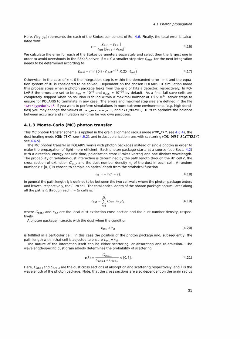
4.1 Photon propagation
Here, f (tk , yk ) represents the each of the Stokes component of Eq. 4.6. Finally, the total error is calcu-lated with:
ε =| yk+1 − yk+1 |
εerr | yk+1 + εabs |. (4.16)
We calculate the error for each of the Stokes parameters separately and select then the largest one inorder to avoid overshoots in the RFK45 solver. If ε > 0 a smaller step size `new for the next integrationneeds to be determined according to
`new = min(0.9 · `oldε
−0.2; 0.25 · `old
). (4.17)
Otherwise, in the case of ε ≤ 0 the integration step is within the demanded error limit and the equa-tion system of RT is considered to be solved. Dependent on the chosen POLARIS RT simulation modethis process stops when a photon package leaks from the grid or hits a detector, respectively. In PO-LARIS the errors are set to be εerr = 10−6 and εabs = 10−30 by default. As a final fail save cells arecompletely skipped when no solution is found within a maximal number of 1.5 × 10⁶ solver steps toensure for POLARIS to terminate in any case. The errors and maximal step size are defined in the file'src/typedefs.h'. If you want to perform simulations in more extreme environments (e.g. high densi-ties) you may change the values of rel_err, abs_err, and MAX_SOLVER_STEPS to optimize the balancebetween accuracy and simulation run-time for you own purposes.
4.1.3 Monte-Carlo (MC) photon transfer
This MC photon transfer scheme is applied in the grain alignment radius mode (CMD_RAT, see 4.6.4), thedust heating mode (CMD_TEMP, see 4.6.2), and in dust polarization runs with scattering (CMD_DUST_SCATTERING,see 4.6.5).
The MC photon transfer in POLARIS works with photon packages instead of single photon in order tomake the propagation of light more efficient. Each photon package starts at a source (see Sect. 4.2)with a direction, energy per unit time, polarization state (Stokes vector) and one distinct wavelength.The probability of radiation-dust interaction is determined by the path length through the i th cell ` , thecross section of extinction Cext, and the dust number density nd of the dust in each cell. A randomnumber z ∈ [0, 1) is chosen to sample an optical depth from the statistical function
τst = − ln(1 − z ). (4.18)
In general the path length `i is defined to be between the two cell walls where the photon package entersand leaves, respectively, the i −t h cell. The total optical depth of the photon package accumulates alongall the paths `i through each i − t h cells is:
τext =N∑i=1
Cext,i nd,i `i. (4.19)
where Cext,i and nd,i are the local dust extinction cross section and the dust number density, respec-tively.
A photon package interacts with the dust when the condition
τext < τst (4.20)
is fulfilled in a particular cell. In this case the position of the photon package and, subsequently, thepath length within that cell is adjusted to ensure τext = τst.
The nature of the interaction itself can be either scattering, or absorption and re-emission. Thewavelength-specific dust grain albedo determines the probability of scattering,
a(λ) = Csca,λ
Cabs,λ + Csca,λ∈ [0, 1]. (4.21)
Here, Cabs,λand Csca,λ are the dust cross sections of absorption and scattering,respectively, and λ is thewavelength of the photon package. Note, that the cross sections are also dependent on the grain radius
31
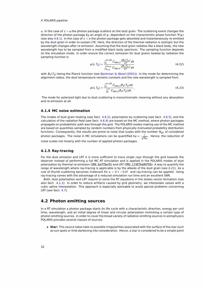
4 POLARIS pipeline
a. In the case of z > a the photon package scatters on the dust grain. The scattering event changes thedirection of the photon package by an angle of ψ, dependent on the characteristic phase function Ψ(ψ)(see also 4.6.1). In the case of z < a the photon package gets absorbed and instantaneously re-emittedby the dust grain in order to sustain LTE. Here, the direction of the thermal radiation is isotropic but thewavelength changes after re-emission. Assuming that the dust grain radiates like a black body, the newwavelength has to be sampled from a modified black body spectrum. The sampling function dependson the simulation mode. In order ensure the correct remission for dust grains heated by radiation thesampling function is
p(λ,Td) =∫ λ+dλλ
Cabs,λdBλ (Td,i)dT dλ∫ λmax
λminCabs,λ
dBλ (Td,i)dT dλ
(4.22)
with Bλ(Td) being the Planck function (see Bjorkman & Wood (2001)). In the mode for determining thealignment radius, the dust temperature remains constant and the new wavelength is sampled from
p(λ,Td) =∫ λ+dλλ
Cabs,λBλ(Td)dλ∫ ∞0Cabs,λBλ(Td)dλ
, (4.23)
The mode for polarized light due to dust scattering is monochromatic meaning without any absorptionand re-emission at all.
4.1.4 MC noise estimation
The modes of dust grain heating (see Sect. 4.6.2), polarization by scattering (see Sect. 4.6.5), and thecalculation of the radiation field (see Sect. 4.6.4) are based on the MC method, where photon packagespropagate on probabilistic path was through the grid. The POLARIS modes making use of the MC methodare based on quantities sampled by random numbers from physically motivated probability distributionfunctions. Consequently, the results are prone to noise that scales with the number Nph of considered
photon packages. The noise in MC simulations can be quantified by ∝ 1√Nph
. Hence, the reduction of
noise scales not linearly with the number of applied photon packages.
4.1.5 Ray-tracing
For the dust emission and LRT it is more sufficient to trace single rays through the grid towards theobserver instead of performing a full MC RT simulation and is applied in the POLARIS modes of dustpolarization by thermal re-emission (CMD_RAYTRACE) and LRT (CMD_LINETRANSFER). A way to quantify therange of wavelength where ray-tracing is applicable is by the albedo of the dust grain (see 4.21). As arule of thumb scattering becomes irrelevant for a < 0.1 − 0.01 and ray-tracing can be applied. Usingray-tracing comes with the advantage of a reduced simulation run time and an excellent SNR.
Both, dust polarization and LRT require to solve the RT equations in the stokes vector formalism (seealso Sect. 4.1.1). In order to reduce artifacts caused by grid geometry, we interpolate values with acubic spline interpolation. This approach is especially advisable to avoid special problems concerningLRT (see Sect. 4.7).
4.2 Photon emitting sources
In a RT simulation a photon package starts its life cycle with a characteristic direction, energy per unittime, wavelength, and an initial degree of linear and circular polarization mimicking a certain type ofphoton emitting sources. In order to cover the broad variety of radiation emitting sources in astrophysicsPOLARIS provides several classes of sources.
• Star: This source takes take no possible irregularities associated with the surface of the star suchas sun spots or limb darkening into consideration. Hence, a star is considered to be a simple point
32
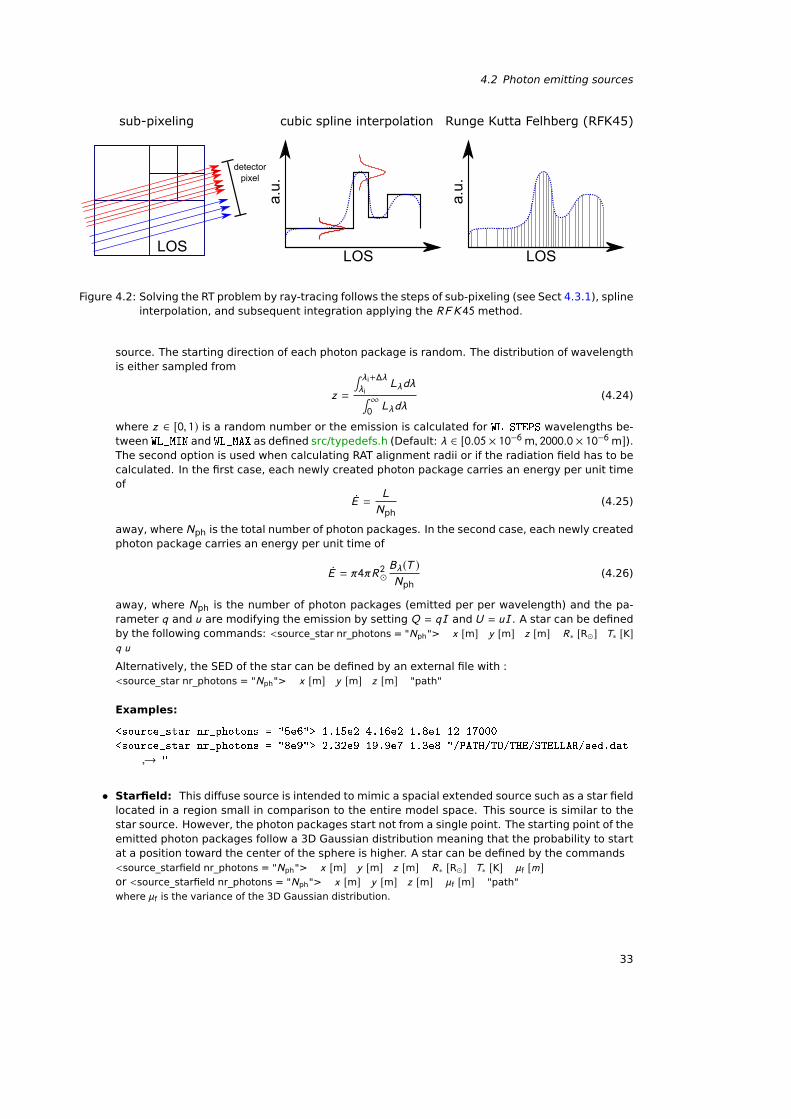
4.2 Photon emitting sources
a.u.
LOS
a.u.
LOS
sub-pixeling cubic spline interpolation Runge Kutta Felhberg (RFK45)
detectorpixel
LOS
Figure 4.2: Solving the RT problem by ray-tracing follows the steps of sub-pixeling (see Sect 4.3.1), splineinterpolation, and subsequent integration applying the RF K45 method.
source. The starting direction of each photon package is random. The distribution of wavelengthis either sampled from
z =
∫ λi+∆λλi
Lλdλ∫ ∞0Lλdλ
(4.24)
where z ∈ [0, 1) is a random number or the emission is calculated for WL_STEPS wavelengths be-tween WL_MIN and WL_MAX as defined src/typedefs.h (Default: λ ∈ [0.05 × 10⁻⁶ m, 2000.0 × 10−6 m]).The second option is used when calculating RAT alignment radii or if the radiation field has to becalculated. In the first case, each newly created photon package carries an energy per unit timeof
ÛE =L
Nph(4.25)
away, where Nph is the total number of photon packages. In the second case, each newly createdphoton package carries an energy per unit time of
ÛE = π4πR2Bλ(T )Nph
(4.26)
away, where Nph is the number of photon packages (emitted per per wavelength) and the pa-rameter q and u are modifying the emission by setting Q = qI and U = uI . A star can be definedby the following commands: <source_star nr_photons = "Nph"> x [m] y [m] z [m] R∗ [R] T∗ [K]q u
Alternatively, the SED of the star can be defined by an external file with :<source_star nr_photons = "Nph"> x [m] y [m] z [m] "path"
Examples:
<source_star nr_photons = "5e6"> 1.15e2 4.16e2 1.8e1 12 17000
<source_star nr_photons = "8e9"> 2.32e9 19.9e7 1.3e8 "/PATH/TO/THE/STELLAR/sed.dat
→ "
• Starfield: This diffuse source is intended to mimic a spacial extended source such as a star fieldlocated in a region small in comparison to the entire model space. This source is similar to thestar source. However, the photon packages start not from a single point. The starting point of theemitted photon packages follow a 3D Gaussian distribution meaning that the probability to startat a position toward the center of the sphere is higher. A star can be defined by the commands<source_starfield nr_photons = "Nph"> x [m] y [m] z [m] R∗ [R] T∗ [K] µf [m]or <source_starfield nr_photons = "Nph"> x [m] y [m] z [m] µf [m] "path"
where µf is the variance of the 3D Gaussian distribution.
33
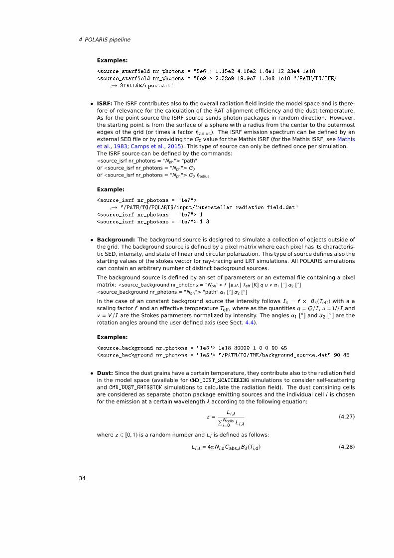
4 POLARIS pipeline
Examples:
<source_starfield nr_photons = "5e6"> 1.15e2 4.16e2 1.8e1 12 23e4 1e18
<source_starfield nr_photons = "8e9"> 2.32e9 19.9e7 1.3e8 1e18 "/PATH/TO/THE/
→ STELLAR/spec.dat"
• ISRF: The ISRF contributes also to the overall radiation field inside the model space and is there-fore of relevance for the calculation of the RAT alignment efficiency and the dust temperature.As for the point source the ISRF source sends photon packages in random direction. However,the starting point is from the surface of a sphere with a radius from the center to the outermostedges of the grid (or times a factor fradius). The ISRF emission spectrum can be defined by anexternal SED file or by providing the G0 value for the Mathis ISRF (for the Mathis ISRF, see Mathiset al., 1983; Camps et al., 2015). This type of source can only be defined once per simulation.The ISRF source can be defined by the commands:<source_isrf nr_photons = "Nph"> "path"
or <source_isrf nr_photons = "Nph"> G0or <source_isrf nr_photons = "Nph"> G0 fradius
Example:
<source_isrf nr_photons = "1e7">
→ "/PATH/TO/POLARIS/input/interstellar_radiation_field.dat"
<source_isrf nr_photons = "1e7"> 1
<source_isrf nr_photons = "1e7"> 1 3
• Background: The background source is designed to simulate a collection of objects outside ofthe grid. The background source is defined by a pixel matrix where each pixel has its characteris-tic SED, intensity, and state of linear and circular polarization. This type of source defines also thestarting values of the stokes vector for ray-tracing and LRT simulations. All POLARIS simulationscan contain an arbitrary number of distinct background sources.
The background source is defined by an set of parameters or an external file containing a pixelmatrix: <source_background nr_photons = "Nph"> f [a .u .] Teff [K] q u v α1 [] α2 []<source_background nr_photons = "Nph"> "path" α1 [] α2 []In the case of an constant background source the intensity follows Iλ = f × Bλ(Teff) with a ascaling factor f and an effective temperature Teff, where as the quantities q = Q/I , u = U/I ,andv = V /I are the Stokes parameters normalized by intensity. The angles α1 [] and α2 [] are therotation angles around the user defined axis (see Sect. 4.4).
Examples:
<source_background nr_photons = "1e5"> 1e18 30000 1 0 0 90 45
<source_background nr_photons = "1e5"> "/PATH/TO/THE/background_source.dat" 90 45
• Dust: Since the dust grains have a certain temperature, they contribute also to the radiation fieldin the model space (available for CMD_DUST_SCATTERING simulations to consider self-scatteringand CMD_DUST_EMISSION simulations to calculate the radiation field). The dust containing cellsare considered as separate photon package emitting sources and the individual cell i is chosenfor the emission at a certain wavelength λ according to the following equation:
z =Li ,λ∑Ncells
i=0Li ,λ
(4.27)
where z ∈ [0, 1) is a random number and Li is defined as follows:
Li ,λ = 4πNi ,dCabs,λBλ(Ti ,d) (4.28)
34
4.2 Photon emitting sources
The photon package starts from a random position evenly distributed in the entire cell volume.Since the photons packages are sampled over all cells via the total dust emission, the energy perunit time and wavelength of an individual photon package is determined by the dust propertieswith a modified black body spectrum as follows:
ÛEλ =4π
Nph
Ncells∑i=0
Ni ,dCabs,λBλ(Ti ,d) (4.29)
where Ni ,d is the number of dust grains in the cell i . The dust as a source of radiation can simplyswitched on and off by writing the tag<source_dust nr_photons = "Nph">
In the command file where Nph defines the number of photon packages to be emitted from eachcell.
Example:
<source_dust nr_photons = "1e6">
• Laser: The laser radiation source is a very narrow band emission source with a normal distri-bution as the emission profile. It is designed for testing models or applications in other fields ofphysics (like plasma physics). It is available for CMD_DUST_EMISSION and CMD_DUST_SCATTERING
simulations. The emitted flux at a wavelength λ can be calculated with the following equation:
Fλ =P√2πσ2
exp
(−(λ − λ0)
2
2σ2
). (4.30)
where P is the total power of the laser (in Watts)m λ0 is the central wavelength, and σ is thestandard deviation that is calculated from the FWHM with the following equation:
σ =FWHM
8 ln(2) . (4.31)
The laser is located at the position x , y , z and points in the direction dx , dy , dz . The laser as asource of radiation can simply switched on and off by writing the tag<source_laser nr_photons = "Nph"> x [m] y [m] z [m] dx [m] dy [m] dz [m] P [W] λ0 [m]FWHM [m] q u
In the command file where Nph defines the number of photon packages to be emitted from eachcell. The parameter q and u are modifying the emission by setting Q = qI and U = uI .
Example:
<source_laser nr_photons = "1e6"> 0 0 0 0 0 0 1e-3 1e-6 1e-9 0 0
HINTS:
• The external file for the SED is a simple table in the form#λ [m] Lλ [W/m]... ...... ...... ...
• The external file for the matrix of the background source is a simple table in the form#λ [m] Lλ [W/m] q u v
... ...
... ...
... ...
35
4 POLARIS pipeline
• A background source is required for any RT simulation based on ray-tracing. If no backgroundsource was defined in the command file a default source will automatically be created with allparameters set to zero.
• The star source can also be used to add the direct attenuated emission of a star to a ray-tracingsimulation (e.g. if the scattered light is considered in ray-tracing simulations via the radiationfield).
• The range of wavelengths has to be equal or larger than the wavelength range defined in thesrc/typedefs.h (Default: λ ∈ [0.05 × 10⁻⁶ m, 2000.0 × 10−6 m]). This range can be adjusted bychanging WL_MIN, WL_MAX, and WL_STEPS in the src/typedefs.h file (use./install_polaris.sh -u afterwards). Intermediate values are calculated by means of cubicspline interpolation.
4.3 Optimization techniques
A 3D MC RT simulation is challenging concerning run time and the capabilities of available computationalequipment. For this reason POLARIS is equipped with several optimization algorithms to perform RTcalculations on a reasonable time and a high SNR.
4.3.1 Sub-pixeling
Using only one ray per detector pixel one may lose information of sub-structures in the model smallerthan the size of of the bin (see Fig. 4.2). In POLARIS each detector pixel starts with four rays as a firststep. Here, POLARIS keeps track of the exact cells the ray passes. If two neighboring rays pass exactlythe same cells the rays are combined to a single ray. In the opposite case, when neighboring rays passdifferent cells each ray is again split into four sub-rays. Since no RT equations are solved in this step,the splitting of rays comes with almost no additional time. Once, the optimal number of rays per pixelis known POLARIS starts with the ray-tracing along each ray. However, allowing POLARIS to split raysdown to the smallest sizes can result in an enormous slow down for the actual ray-tracing since the RTproblem needs to be solve for all the rays separately. Hence, it is recommended to limit the maximallevel of splitting. The command is:<max_subpixel_lvl> Nspl i t
Hence, each detector pixel gets hit by a maximal number of 4Nsplit rays. When the sub-pixel level isnot set the level is 3 by default.
Example:
<max_subpixel_lvl> 3
HINTS:
• For spherical or cylindrical grids, the usage of the polar ray-tracing detector is recommended.The amount of rays is arranged to fit to the spherical or cylindrical distribution of cells.Subsequently, the Stokes vector in each map pixel is calculated by 2D interpolation. To use thepolar ray-tracing grid, simply use detector_dust_polar instead of detector_dust. For moredetails, see Sect. 4.5.
4.3.2 Enforced first scattering
In optically thin regions an interaction between dust and radiation is highly unlikely and a significantlyhigh amount of photon packages can escape the grid without any interaction at all. In POLARIS thephoton package can be forced to interact at least once with the dust according to the method presentedin Cashwell (1957) in order to increase the SNR. For each newly created photon package, an optical
36
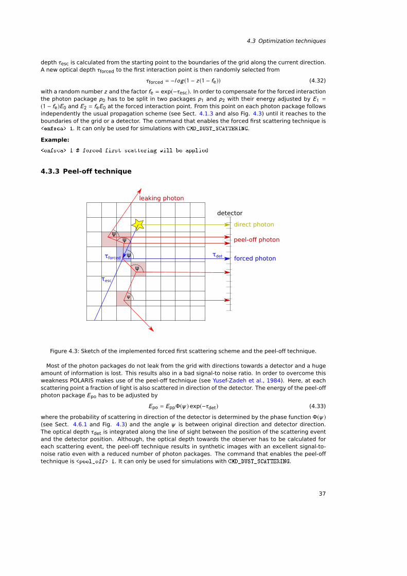
4.3 Optimization techniques
depth τesc is calculated from the starting point to the boundaries of the grid along the current direction.A new optical depth τforced to the first interaction point is then randomly selected from
τforced = −l og (1 − z (1 − fe)) (4.32)
with a random number z and the factor fe = exp(−τesc). In order to compensate for the forced interactionthe photon package p0 has to be split in two packages p1 and p2 with their energy adjusted by E1 =(1 − fe)E0 and E2 = feE0 at the forced interaction point. From this point on each photon package followsindependently the usual propagation scheme (see Sect. 4.1.3 and also Fig. 4.3) until it reaches to theboundaries of the grid or a detector. The command that enables the forced first scattering technique is<enfsca> 1. It can only be used for simulations with CMD_DUST_SCATTERING.
Example:
<enfsca> 1 # forced first scattering will be applied
4.3.3 Peel-off technique
leaking photon
peel-off photon
forced photon
direct photon
detector
ψ
ψ
ψ
ψψ
τesc
τdetτforced
Figure 4.3: Sketch of the implemented forced first scattering scheme and the peel-off technique.
Most of the photon packages do not leak from the grid with directions towards a detector and a hugeamount of information is lost. This results also in a bad signal-to noise ratio. In order to overcome thisweakness POLARIS makes use of the peel-off technique (see Yusef-Zadeh et al., 1984). Here, at eachscattering point a fraction of light is also scattered in direction of the detector. The energy of the peel-offphoton package Epo has to be adjusted by
Epo = EppΦ(ψ) exp(−τdet) (4.33)
where the probability of scattering in direction of the detector is determined by the phase function Φ(ψ)(see Sect. 4.6.1 and Fig. 4.3) and the angle ψ is between original direction and detector direction.The optical depth τdet is integrated along the line of sight between the position of the scattering eventand the detector position. Although, the optical depth towards the observer has to be calculated foreach scattering event, the peel-off technique results in synthetic images with an excellent signal-to-noise ratio even with a reduced number of photon packages. The command that enables the peel-offtechnique is <peel_off> 1. It can only be used for simulations with CMD_DUST_SCATTERING.
37
4 POLARIS pipeline
Example:
<peel_off> 1 # forced first scattering will be applied
4.3.4 Wavelength range selection
Stars and star fields emit photons in the full wavelength range of its black body SED which depends onits characteristic temperature. However, wavelengths at both ends of the SED can be neglected sincethey do not contribute significantly to the total emitted energy of the source. This reduces the numberof wavelength to be considered and subsequently the computational efforts. POLARIS adjusts the SEDof any source automatically so that maximal 10−6% of the total luminosity gets lost. This technique isstandard in POLARIS and can not be switched off. However, if the radiation field has to be saved in thegrid by using <radiation_field> 1, each wavelength will be used and no wavelength will be neglected.
4.4 Grid rotation
The grid is by default orientated in an external coordinate system with the xy-plane towards the observerand the z-axis along the LOS. In order to re-orientate the grid for dust scattering, dust ray-tracing, orline RT two arbitrary rotation axis can be defined.
<axis1> x [a.u.] y [a.u.] z [a.u.]
<axis2> x [a.u.] y [a.u.] z [a.u.]
By default the first rotation axis the x-axis (100) and the second rotation axis is along the y-axis (001).Examples:
<axis1> 1 0 0 # defining the x axis as first rotation axis
<axis2> 1 1 1 # defining a diagonal direction as second rotation axis
Later, these rotation axis define the orientation of the grid with respect to the detector (see 4.5).
HINTS:
• The vectors defining the two axis will automatically be normalized.
• Both rotation axes are independent from each other and do not rotate itself around the rotationangle.
4.5 Detector parameters
The POLARIS code provides two main classes of detectors. The plane detector and the spherical (healpix)detector. The plane detector should be used when the observer is far away from the grid and the rayscan be considered to be parallel from each other. This kind of detector is available for MC dust scatter-ing (CMD_DUST_SCATTERING), ray-tracing for thermal emission of dust grains (CMD_DUST_EMISSION), LRT(CMD_LINETRANSFER), and synchrotron RT (CMD_SYNCHROTRON). A plane detector is characterized by itsdistance, viewing angles, wavelength, and the number of pixel. The exact command for a detectordepends on the kind of POLARIS simulation mode.
For observations considering dust scattering (CMD_DUST_SCATTERING) a plane detector is defined by:
<detector_dust_mc nr_pixel = "Npixel"> λmin λmax Nλ α1 [deg] α2 [deg] D [m]
where Npixel is the number of pixel, λmin is the shortest wavelength, λmax is the longest wavelength,Nλis the amount of wavelengths used for simulation (if 1, only λmin is used), α1 and α2 are the rotationangles around the first and second rotation axis (see Sect. 4.4), and D is the distance to the observer.
An optional feature is the zoom of the detector. This can be done by adding the desired side-lengthsto the command line (available for each plane detector).
38
4.5 Detector parameters
<detector_dust_mc nr_pixel = "Npixel"> ... dx [m] dy [m]
Another optional feature is the definition of individual numbers of pixel for each direction (availablefor each plane detector).
<detector_dust_mc nr_pixel = "Npixel,x*Npixel,y"> ...
Examples:
<detector_dust_mc nr_pixel = "256"> 1e-6 2e-6 2 15.1 0 4.31998E+18
<detector_dust_mc nr_pixel = "256*128"> 1e-6 1e-5 2 35.1 0 4.31998E+18 149597870700.0
→ 149597870700.0
For observations considering ray-tracing of the dust thermal emission (CMD_DUST_EMISSION) a planedetector is defined by:
<detector_dust nr_pixel = "Npixel"> λmin λmax Nλ IDsource α1 [deg] α2 [deg] D [m]
The only difference to the scattering detector is the definition of IDsource. This ID is related to the indexof the defined background sources (has to be 1, if no background source is defined). In contrast to thescattering detector, the ray-tracing detectors can make use of a background grid that is not the sameas the used 2D Cartesian pixel map. Other options are 'polar' or 'slice'. They are chosen by writing<detector_dust_polar or <detector_dust_slice. The 'polar' grid can only be used if the underlying3D grid is spherical or cylindrical and it should be used if the 3D grid contains a lot of cell close to thecenter (fr > 1.0). The 'slice' background grid has only a analyzing purpose. Here, the 2D Cartesianbackground grid is put inside of the grid as a horizontal slice. Each ray-tracing pixel starts at differentpositions in the grid. For instance, this can be used to create contour height plots of the optical depth.
In addition to the zoom feature, the ray-tracing detector can also be shifted in both directions. Thiscan be done by adding the desired shift of the detector to the command line.
<detector_dust nr_pixel = "Npixel"> ... dx [m] dy [m] ∆x [m] ∆y [m]
Examples:
<detector_dust nr_pixel = "256"> 1e-6 2e-6 2 1 15.1 0 4.31998E+18
<detector_dust nr_pixel = "256*128"> 1e-6 2e-6 2 1 35.1 0 4.31998E+18 149597870700.0
→ 149597870700.0 14959787070.0 -14959787070.0
<detector_dust_polar nr_pixel = "256"> 1e-6 2e-6 2 1 35.1 0 4.31998E+18
<detector_dust_slice nr_pixel = "256"> 1e-6 2e-6 2 1 35.1 0 4.31998E+18
For observations considering ray-tracing of the spectral line emission (CMD_LINE_EMISSION) a planedetector is defined by:
<detector_line nr_pixel = "Npixel" vel_channels = "Nvel"> IDgas species IDtransition IDsource→ vmin,max [m/s] α1 [deg] α2 [deg] D [m]
where Nvel is the number of the applied velocity bins, IDgas species is the ID of a gas species (atom/-molecules) previously defined in the command file, IDtransition is the ID of the line transition correspond-ing to the ID in the Leiden molecular database file (see Sect. 3.5), and vmin,max defines the upper andlower limits of the velocity range.
Examples:
<detector_line nr_pixel = "256" vel_channels = "35"> 1 2 1 1e5 15.1 0 4.31998E+18
<detector_line nr_pixel = "256*128" vel_channels = "101"> 1 5 1 1e5 35.1 0 4.31998E+18
→ 149597870700.0 149597870700.0 14959787070.0 -14959787070.0
<detector_line_polar nr_pixel = "256" vel_channels = "35"> 1 5 1 1e5 35.1 0 4.31998E+18
<detector_line_slice nr_pixel = "256" vel_channels = "101"> 1 5 1 1e5 35.1 0 4.31998E+18
39
4 POLARIS pipeline
HINTS:
• Use an odd number of velocity bins Nvel to ensure to observe at the exact transition frequencyνij
Defining a detector for a POLARIS synchrotron run is similar to the definition of a dust detector for ray-tracing. For observations considering synchrotron emission and Faraday rotation (CMD_SYNCHROTRON) aplane detector is defined by:
<detector_sync nr_pixel = "Npixel"> λmin λmax Nλ IDsource α1 [deg] α2 [deg] D [m]
The zoom feature of the synchrotron detector as well as the shifting in both directions can be definedby:
<detector_sync nr_pixel = "Npixel"> ... dx [m] dy [m] ∆x [m] ∆y [m]
Examples:
<detector_sync nr_pixel = "256"> 0.71 0.81 2 1 15.1 0 4.31998E+18
<detector_sync nr_pixel = "256*128"> 0.71 0.81 2 35.1 0 4.31998E+18 149597870700.0
→ 149597870700.0 14959787070.0 -14959787070.0
A spherical detector should be used when the observer has a position within the grid and the rays arecoming from the outside (a surrounding sphere). This kind of detector is not yet available for the dustscattering mode and is purely based on ray-tracing.
For spherical detectors the ray-tracing starts from of a sphere with a diameter that is larger than theside length of the grid and ends at the exact position of the observer. The starting points are equallydistributed on the surface of the sphere according to the HEALPIX pixelation 1. This makes the POLARISspherical detector directly comparable to Planck data and comes with the advantage that each point onthe sphere is surrounded the same surface area.
In order to perform ray-tracing with aligned dust grains, the spherical detector can be defined by:
<detector_dust_healpix nr_sides = "Nsides"> λmin λmax Nλ IDsource rx [m] ry [m] rz [m]
→ lmin [deg] lmax [deg] bmin [deg] bmax [deg]
Here, rx , ry , and rz is the position of the observer within the grid and Nsides defines the number of sidesaccording to the HEALPIX algorithm. The HEALPIX algorithm requires for the number of sides Nsides to beto the base of 2 e.g. 1, 2, 4, 8 .... The total number of detector pixel is then defined by Npixel = 12 N
2sides.
By default the spherical detector covers the full sky and points in direction of the center of the grid.The quantities lmin, lmax, bmin, and bmax are optional and define the minimum and maximum of thelongitude and latitude, respectively, of the area on the sphere to be observed. However, in contrast tothe galactic coordinate system the angles are defined to be l ∈ [−180, 180] and b ∈ [−90, 90].
Example:
<detector_dust_healpix nr_sides = "32"> 1e-6 1e-5 2 1 1.65e+20 0 0 -80 80 -45 45
A LRT detector is defined by:
<detector_line_healpix nr_sides = "Nsides" vel_channels = "Nvel"> IDgas species IDtransitionIDsource vmin,max [m/s] rx [m] ry [m] rz [m] lmin [deg] lmax [deg] bmin [deg] bmax [
→ deg] vx [m/s] vy [m/s] vz [m/s]
Here, the quantities vx vy, and vz are also optional and define the velocity of the observer relative to thegrid.
Example:
1https://healpix.jpl.nasa.gov
40
4.6 Dust continuum radiative transfer
<detector_line_healpix nr_sides = "32" vel_channels = "35"> 1 2 1 1e5 1.96e+20 0 0 -180
→ 180 -3.5 3.5 1.5e3 -1e3 0
Following our previous scheme, the HEALPIX synchrotron detector is defined by:
<detector_sync_healpix nr_sides = "Nsides"> λmin λmax Nλ IDsource rx [m] ry [m] rz [m]
→ lmin [deg] lmax [deg] bmin [deg] bmax [deg]
Example:
<detector_sync_healpix nr_sides = "512"> 0.03 0.7 11 1.65e+20 0 0 -80 80 -45 45
4.6 Dust continuum radiative transfer
4.6.1 Phase functions
Light propagating through a dusty medium will change its direction by scattering on a single dust grains.The angular distribution of scattering on a grain at a given wavelength is given by the phase functionφ. Many phase functions have been proposed to account for dust with different shapes, sizes, andproperties of grain materials. POLARIS allows to choose the kind of phase function used in the differentMC based modes.
• Isotropic scattering:In the case of isotropic scattering each direction has the same probability after the scatteringevent. The same sampling process is also applied by the thermal remission. The new photonpackage direction ®r ′ is sampled from a uniform distribution of points on the surface of a unit
sphere and depends on the three parameters u = 1 − 2z1, t = 2πz2, and r =√1 − u2 and can be
calculated by
®r ′ = (r cos(t ), r sin(t ),u)T . (4.34)
Here, the quantities z1 and z2 are random numbers. This phase function is available for all MCbased POLARIS modes. In order to activate isotropic scattering the line
<phase_function> PH_ISO
needs to be in the command file.
• Anisotropic scattering:In contrast to isotropic scattering, anisotropic scattering is characterized by a preferential scatter-ing directions. The Henyey-Greenstein (HG) phase function is the most widely used parametriza-tion of the phase function and provides a good single-parameter approximation with
φ(ψ) = 1
4π
1 − g 2[1 + g 2 − 2 ∗ cos(ψ)] 32 . (4.35)
This phase function depends on scattering angle ψ and the asymmetry parameter g ∈ [−1, 1]where g = 0 means isotropic scattering, g = 1 backward scattering, and g = 1 forward scattering,respectively. The anisotropy parameter g is pre-calculated dependent on material, grain size,and wavelength, and provided by the dust parameters file (Sect. 3.4). The HG phase functioncan be selected with:
<phase_function> PH_HG
41
4 POLARIS pipeline
The HG phase function is the standard phase function.In the case of homogeneous and spherical dust grains a solution to the scattering problem canbe found with Mie scattering theory. Here, the phase function of scattering can be expanded interms of an infinite series of associated Legendre polynomials. The coefficients of the series canbe calculated with the refractive index of the dust grain material. This allows to calculate thenew scattering direction by utilizing the pre-calculated values of the scattering matrix. The S11element of the scattering matrix can be used by POLARIS to calculate the phase function (see4.6.5 for details). The Mie scattering phase function is only available for the MC dust polarizationmode and can be activated by
<phase_function> PH_MIE
A MC mode with scattering on non-spherical dust grains is currently in development.
4.6.2 Dust heating
The command that identifies the dust heating mode is CMD_TEMP. This mode is a combination of themethods of continuous absorption Lucy (1999) and immediate re-emission Bjorkman & Wood (2001).As a minimal requirement the input grid needs the 3D gas density distribution. Additionally, a dustmodel and at least one photon emitting source is required. However, if the grid contains no furtherphysical parameters, no follow-up RT calculations (e.g. dust polarization) are possible. The dust shapeand the possible alignment of non-spherical dust grains has no influence on the resulting dust dusttemperature distribution. For this POLARIS mode the dust grains are considered to be spherical in thedust heating mode. This reduces the required computational efforts dramatically.
In the beginning of the dust heating mode the emissivity
jI(Td) = nd
∫Cabs,λBλ(Td)dλ (4.36)
is pre-calculated for a range of dust temperaturesTd ∈ [1 K, 4000 K] and tabulated. Each photon packagestarts with an energy per unit time ε/∆t and a wavelength λ. In each cell with volumeVcell, we store theenergy per unit time
ÛE = ndε
Vcell∆t
∑i
Cabs,λi× l i + ∆ ÛE (4.37)
that all passing photon packages deposit along their paths l during the MC dust heating simulation. Thequantity ∆ ÛE describes the offset in the dust heating simulation in the case of an already exiting dusttemperature.If the photon package interacts by means of absorption and re-emission (see also 4.1.3) a new wave-length is sampled from
z =
∫ λiλmin
Cabs,λdBλ (Td,i)dT dλ∫ λmax
λminCabs,λ
dBλ (Td,i)dT dλ
(4.38)
to LTE . Since the temperature changes by each absorption event the new wavelength cannot be sam-pled from the Planck function but by its temperature derivative in order to ensure a correct spectrumof the emitted photons (compare Eq. 4.23). Finally, we compare ÛE with the tabulated and cubic splineinterpolated values of j (Td) in the end of the MC simulation in order to determine the dust temperatureTd. The newly calculated grid ('grid_temp.dat') will the be stored in the defined output directory. If thegrid contains no dust temperature at all the grid will be extended by one additional physical parameter.
We provide a minimal example command file for the dust heating mode in Listing 4.1. As a radi-ation source a single solar like star at the center of the grid is defined sending 106 photon packagesinto the grid. The dust model consists only of silicate grains. Besides the path to the dust parame-ters file, no further parameters are defined. This means we consider the full size range with an sizedistribution exponent of q = −3.5 for the dust model. Again, we define the path of the input grid andthe path for the resulting grid and additional output files (e.g. plots). In this simulation we use themaximal possible number of threads of the machine (<nr_threads> -1). For the dust-to-gas mass ratio
42
4.6 Dust continuum radiative transfer
we use the usual value of 1%. POLARIS can not directly calculate a gas temperature. However, a fixedratio of gas temperature Td to dust temperature Td can be assumed with the command <adj_tgas>.Any possible input gas temperature is lost if this command is defined. If stochastic heating should beconsidered for the thermal emission of the dust grains, either the radiation field or the effective tem-perature due to stochastic heating has to be saved in the grid with the command <radiation_field> 1
or <stochastic_heating> SIZE_LIMIT. Saving the radiation field offers more flexibility and precision,since the probability distribution of temperatures will be used in the dust emission and the maximumsize can be varied between each dust emission simulation. However, saving the radiation field signifi-cantly increases the grid memory size (by around 400 doubles per cell) and the calculation of the dustemission takes more time if the stochastic heating is considered by using the probability distribution oftemperatures that is calculated out of the radiation field.
Additionally, a dust temperature can also already be contained in the input grid e.g. as a result ofa MHD simulation. This temperature may emerge from different physical processes (e.g. gas-dust col-lisions or compression) other than radiation-dust interaction. Hence, it may be of interest to combineboth dust temperatures by defining the command <dust_offset> (0=off and 1=on). Here, POLARISperforms the reverse calculation by comparing the input dust temperature with the pre-calculated val-ues of j (Td) in order to determine the offset of ∆ ÛE in each cell (see Eq. 4.37). The resulting final dusttemperature is higher as the sum of both separate temperatures.
Instead of only calculating the dust temperature distribution for an average dust grain size, a dusttemperature can be calculated for each dust grain size individually by adding the following command tothe CMD_TEMP simulation:
<full_dust_temp> 1
The resulting temperature containing grid will be adjusted accordingly (see 5.1) and any follow-up sim-ulation of the thermal emission with this grid will use the temperatures of each grain size. As a con-sequence, the considered dust composition cannot not be changed after the temperature calculation(which in general should not be done).
4.6.3 Grain alignment theories
Besides Zeeman splitting the extensive treatment of imperfectly aligned dust grains in the RT simula-tions is one of the unique features of the POLARIS code. A unifying theory of dust grain alignment isstill missing. For this reason POLARIS allows to choose from the major classes of dust grain alignmenttheories developed so far. In this section we intent to provide a short summary about this theories andtheir physical implications.
Considering the violent environment in most astrophysical processes the perfect alignment of non-spherical dust grains with respect to the magnetic field direction is permanently disturbed (see Fig.4.4). This leads to the precession angles of β and ζ. The angle β is defined to be between the angularmomentum of the dust grain ®J and the magnetic field ®B ans ζ is between the maximum moment ofinertia ®I and ®J . The larger the precession angles are the more the non-spherical dust grains appear tobe spherical. Consequently, the resulting polarization becomes reduced. A measurement to quantifythis is the so called Rayleigh reduction factor
R =⟨G
(cos2(β )
)G
(cos2(ζ)
)⟩∈ [0, 1] (4.39)
where R = 1 stands for the maximal possible polarization of a dust grain and R = 0 when polarizationis completely suppressed. The Rayleigh reduction factor is defined by the precession angles averagedover distribution functions whereG (x ) = 1.5x−0.5. In order to reduce the computational time we assumethe precession angles to be mostly independent with
〈G (X )G (Y )〉 ≈ 〈G (X )〉 × 〈G (Y )〉 (1 + fc) . (4.40)
where fc is a correlation factor and fc = 0.6 stands for no correlation at all. For most cases fc ≈ 0.6 andof minor relevance. However, if required it can be changed by the user with the command <f_c> 0.6.
The distribution functions in turn depend heavily on the considered dust grain alignment theory.
43
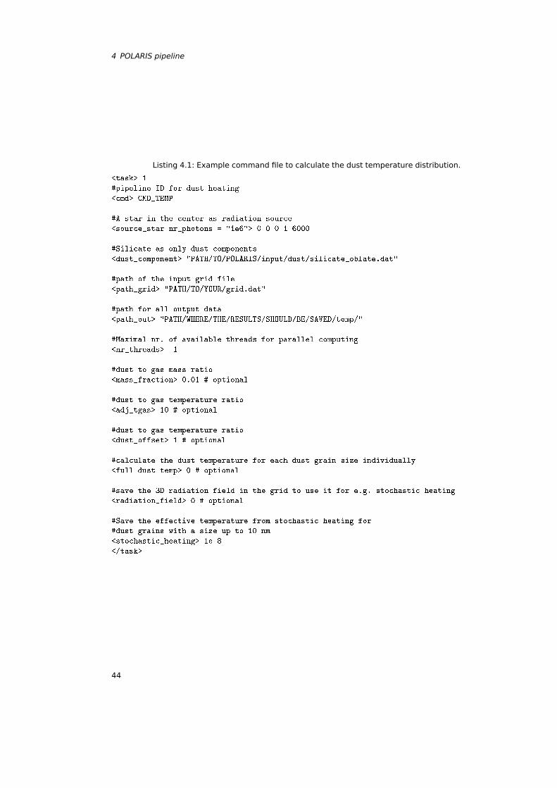
4 POLARIS pipeline
Listing 4.1: Example command file to calculate the dust temperature distribution.
<task> 1
#pipeline ID for dust heating
<cmd> CMD_TEMP
#A star in the center as radiation source
<source_star nr_photons = "1e6"> 0 0 0 1 6000
#Silicate as only dust components
<dust_component> "PATH/TO/POLARIS/input/dust/silicate_oblate.dat"
#path of the input grid file
<path_grid> "PATH/TO/YOUR/grid.dat"
#path for all output data
<path_out> "PATH/WHERE/THE/RESULTS/SHOULD/BE/SAVED/temp/"
#Maximal nr. of available threads for parallel computing
<nr_threads> -1
#dust to gas mass ratio
<mass_fraction> 0.01 # optional
#dust to gas temperature ratio
<adj_tgas> 10 # optional
#dust to gas temperature ratio
<dust_offset> 1 # optional
#calculate the dust temperature for each dust grain size individually
<full_dust_temp> 0 # optional
#save the 3D radiation field in the grid to use it for e.g. stochastic heating
<radiation_field> 0 # optional
#Save the effective temperature from stochastic heating for
#dust grains with a size up to 10 nm
<stochastic_heating> 1e-8
</task>
44
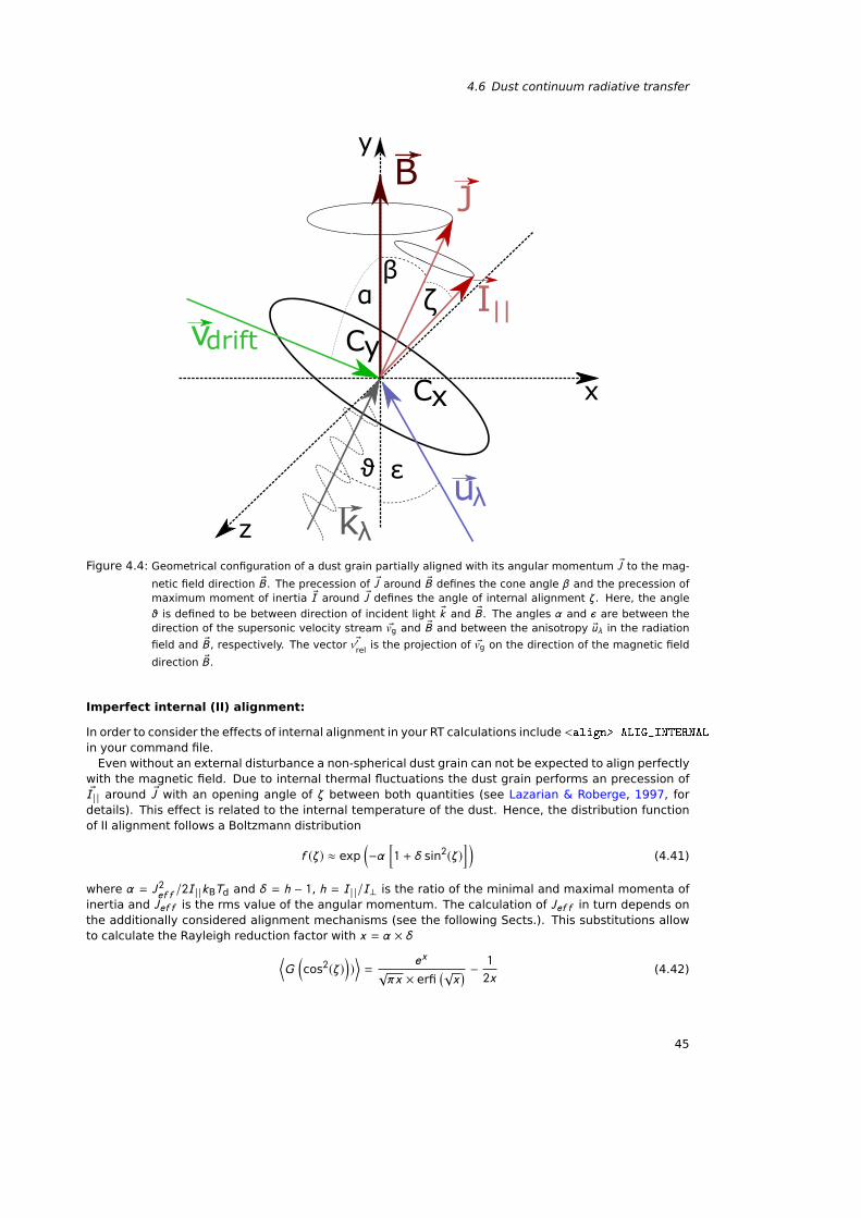
4.6 Dust continuum radiative transfer
x
y
z
βα
ε
BJ
v
λu
I||ζ
ϑ
Cx
Cydrift
λkFigure 4.4: Geometrical configuration of a dust grain partially aligned with its angular momentum ®J to the mag-
netic field direction ®B . The precession of ®J around ®B defines the cone angle β and the precession ofmaximum moment of inertia ®I around ®J defines the angle of internal alignment ζ. Here, the angle
ϑ is defined to be between direction of incident light ®k and ®B . The angles α and ε are between thedirection of the supersonic velocity stream ®vg and ®B and between the anisotropy ®uλ in the radiation
field and ®B , respectively. The vector ®v′rel is the projection of ®vg on the direction of the magnetic field
direction ®B .
Imperfect internal (II) alignment:
In order to consider the effects of internal alignment in your RT calculations include <align> ALIG_INTERNAL
in your command file.Even without an external disturbance a non-spherical dust grain can not be expected to align perfectly
with the magnetic field. Due to internal thermal fluctuations the dust grain performs an precession of®I | | around ®J with an opening angle of ζ between both quantities (see Lazarian & Roberge, 1997, for
details). This effect is related to the internal temperature of the dust. Hence, the distribution functionof II alignment follows a Boltzmann distribution
f (ζ) ≈ exp(−α
[1 + δ sin2(ζ)
] )(4.41)
where α = J 2ef f/2I | |kBTd and δ = h − 1, h = I | |/I⊥ is the ratio of the minimal and maximal momenta of
inertia and Jef f is the rms value of the angular momentum. The calculation of Jef f in turn depends onthe additionally considered alignment mechanisms (see the following Sects.). This substitutions allowto calculate the Rayleigh reduction factor with x = α × δ⟨
G(cos2(ζ)
))⟩=
ex√πx × erfi
(√x) − 1
2x(4.42)
45
4 POLARIS pipeline
Imperfect Davis – Greenstein (IDG) alignment
The IDG can be switched on by adding <align> ALIG_IDG to the command file.This theory provides a steady state solution for dust grain alignment by balancing the disturbances onthe grain by random gas collisions withe alignment effects of paramagnetic relaxation (Davis-Greensteineffect) in the dust grain material (Davis & Greenstein, 1951; Spitzer & McGlynn, 1979). Solving theequations of state the Rayleigh reduction factor can be calculated with
⟨cos2(β )
⟩=
©«1 −√
ξ2(a)1 − ξ2(a)
ª®¬ arcsin
√1 − ξ2(a)1 − ξ2(a) . (4.43)
where
ξ2(a) =a + δ0 × TdTga + δ0
. (4.44)
Here, the critical parameter is
δ0 = 2.07 × 10²⁰ B2
ngTd√Tg, (4.45)
which provides an upper threshold of dust grain alignment. Dust grains with sizes a > δ0 do not con-tribute significantly to polarization. The constant 2.07 × 10²⁰ is adequate for most paramagnetic materi-als. However, it can be changed by the user with the command <delta0>.As for the angular momentum of internal alignment we use the approximation:
J 2ef f ≈√(1 + 0.5s−2
) (1 +Td/Tg
) × (2I | |kBTg
)2. (4.46)
GOLD (magneto mechanical) alignment
The original Gold alignment described only the aligment of dust grains in the presence of a velocityfield (Gold, 1952). Later, this this theory was extended to model also the influence of the magnetic field(magneto mechanical alignment, see Lazarian, 1995; Lazarian et al., 1996; Lazarian & Efroimsky, 1996).For considering GOLD alignment write <align> ALIG_GOLD in your command file.In GOLD alignment two forces act on the dust grain simultaneous caused by an directed gas stream andthe alignment by the magnetic field. This leads to a dependency of dust grain alignment on the angle αbetween the predominate direction of the velocity stream and the magnetic field direction. As a solutionfor the Rayleigh reduction factor the GOLD alignment theory provides
⟨cos2(β )
⟩=
√−g arcsin(
√−s/(1+g ))
s arctan√sg/(1+s+g ) − 1/s if s < 0
√−g sinh−1(√s/(1+g ))
s tanh− 1(√−sg/(1+s+g )) − 1/s if s > 0
(4.47)
with the anisotropy factor of the gas stream
s = −12
〈 ®vrel〉 − 3⟨ ®v′
rel
⟩〈 ®vrel〉 −
⟨ ®v′rel
⟩ (4.48)
Here, ®v′rel
is the projection of the relative drift velocity ®vrel between the gas and dust component on themagnetic field direction and g is a geometrical factor.In order to calculate the II alignment the angular momentum of GOLD alignment can be approximatedby
J 2ef f ≈ kBI | |(2/h + 1)(Tg +Td
2+µmHv
2rel
6kB
)(4.49)
46
4.6 Dust continuum radiative transfer
with the molecular mass µmH of the gas. The GOLD alignment requires an supersonic velocity streamwith a Mach - numberM > 1. Dust grains with smaller number are assumed to be not aligned. Therefore,POLARIS calculates
M =vrel√
kBTg/µmH(4.50)
, for each cell of the grid. The average mass of a gas particle in these calculations can be controlled withthe command <mu>. As for the coupling efficiency between magnetic field and dust grain alignment wedemand: ®B > 4.1 × 10⁻¹⁸a ng√TgTd
s2(4.51)
The same limitation of the magnetic field applies also to RAT alignment. In the case of other dust grainmaterials you can use the command <larm_f> to alter the pref actor of Eq. 4.51.It needs to be emphasized that this model of mechanical alignment turned out to be unreliable andmight be updated on a short term to keep up with current research on that field.
Radiative torque (RAT) alignment
This alignment theory can be switches on with the command <align> ALIG_RAT .The implementation in POLARIS is based on the work presented in Draine & Weingartner (1996), Draine& Weingartner (1997), Weingartner & Draine (2003), Lazarian & Hoang (2007), and Hoang et al. (2018).RAT alignment balances the influences of random gas bombardment, paramagnetic dissipation in thedust grain material, and the radiative pressure due to an isotropic radiation field. In order for thisalignment theory to work efficiently the angular velocity ωgas caused by gas collisions has to be smalleras the angular velocity ωrad because of radiative pressure by a factor of ≈ 3. This ratio can be calculatedby (
ωrad
ωgas
)2=aalgρd
δmH
(tgas
(tgas + t rad)ngkBTg
∫QΓ(ε)λγλuλdλ
)2. (4.52)
where, ρd is the grain material density, δ is a geometry factor, QΓ(ε) is the radiative torque efficiency(see Sect. 3.4), ε is the angle between the predominant direction of radiation and the magnetic field,and the characteristic time scales tgas and t rad are the drag times corresponding to gas drag and thermalemission drag, respectively.The critical quantities here are the local mean energy density uλ is the wavelength specific anisotropy
factor γλ varies between γλ = 1 for an unidirectional radiation field and γλ = 0 for completely isotropicradiation. Both, mean energy density uλ and anisotropy factor γλ can be calculated by POLARIS inan extra RT mode (see 4.6.4). Given that uλ and γλ are known, POLARIS is able to determine thecharacteristic dust grain size aalg at which dust grains start to align (ωrad > ωgas).
An analytically distribution function for the precession angle β and, subsequently, the Rayleigh re-duction factor is unknown so far. However, the Rayleigh reduction factor can be estimated. Solvingthe equations of state reveals two attractor points in the parameters space of RAT theory with differ-ent angular momenta. Dust grains at the attractor point with a high angular momentum (high-J) canbe assumed to aligned perfectly where as the second attractor point is internally not perfectly aligned
or rather⟨G
(cos2(ζ)
)⟩< 1. Defining fhigh−J to be the fraction of dust grains that settle at the high-J
attractor point the Rayleigh reduction factor can be approximated with
R ≈fhigh−J + (1 − fhigh−J)
⟨G
(cos2(ζ)
)⟩if a ≥ aalg
0 if a < aalg
(4.53)
The angular momentum for II alignment is assumed to be J 2ef f≈ 2I | |kBTg. The POLARIS code assumes
a value of fhigh−J = 0.25 however this values can be changed with the command <f_highJ>.
47
4 POLARIS pipeline
Combined of Rayleigh reduction factors
Since all these alignment theories have their place and are most likely simultaneously at work POLARISallows to calculate a combined Rayleigh reduction factor with
R˚ ≈R IDG + RRAT + RGOLD + R IDGRRAT + R IDGRGOLD + RRATRGOLD + 3R IDGRRATRGOLD
1 + 2R IDGRRAT + 2R IDGRGOLD + 2RRATRGOLD + 2R IDGRRATRGOLD(4.54)
However, this is a first approximation and has to be taken with care. In order to combine the alignmenttheories you can list any number of combination of alignment commands in your command file e.g.
<align> ALIG_INTERNAL
<align> ALIG_RAT
<align> ALIG_GOLD
<align> ALIG_IDG
4.6.4 The grain alignment radius aalg
The command that identifies the RAT alignment radius mode is CMD_RAT. In order to solve Eq. 4.52 thelocal mean energy density uλ and the wavelength specific anisotropy factor γλ need to be determined.Here, POLARIS uses a MC mode where we store the direction and magnitude of the energy density ®uλ ineach cell. For the mean energy density per path length and wavelength we derive
®uλ,i =ε
c∆tVcell
®k × l i®k (4.55)
where ®k is the wave vector of of each photon package. This allows to calculate the mean energy density
uλ =
Nph∑i=1
®uλ,i (4.56)
and the anisotropy parameter
γλ =1
uλ
Nph∑i=1
®uλ,i
∈ [0; 1] (4.57)
The RAT alignment radius mode is the most memory demanding one since four values (8 bytes, dou-ble,
(ux,uy,uz
)λ,Z, and uλ) per wavelength and cell need to be stored and updated when a new photon
package passes the cell. Finally, POLARIS solves Eq. 4.52 in order to calculate the minimal dust grainalignment radius aalg in each cell. A new grid will be created that contains all the physical input quanti-ties extended by the alignment radius aalg and stored as 'grid_rat.dat' in the output path. We providea minimal example command file for the RAT alignment mode in Listing 4.2.
POLARIS also allows the calculation of both, the dust temperature and RAT alignment radius at onceby using CMD_TEMP_RAT instead of CMD_TEMP or CMD_RAT. The output grid will be named 'grid_temp.dat'
and includes both quantities.
4.6.5 Dust Intensity and polarization maps
Polarization by non-spherical dust grains
Describing the RT problem without scattering for aligned dust grains in the Stokes vector formalismleads to the following system of equations: Here, nd is the dust number density d l is the infinitesimalpath length element, and Bλ(Td) is the Planck function for a give dust temperature Td.Focusing on extinction the entries of the cross sections matrix can be calculated with:
48
4.6 Dust continuum radiative transfer
Listing 4.2: Example command file to calculate the dust temperature distribution.
<task> 1
#pipeline ID for RAT alignment radius simulation
<cmd> CMD_RAT
#A star in the center as radiation source
<source_star nr_photons = "1e6"> 0 0 0 1 6000
# Silicate as only dust components
<dust_component> "PATH/TO/POLARIS/input/dust/silicate_oblate.dat"
#path of the input grid file
<path_grid> "PATH/WHERE/THE/RESULTS/SHOULD/BE/SAVED/temp/grid_temp.dat"
#path for all output data
<path_out> "PATH/WHERE/THE/RESULTS/SHOULD/BE/SAVED/rat/"
#Maximal nr. of threads for parallel computing
<nr_threads> -1
#dust to gas mass ratio
<mass_fraction> 0.01 # optional
</task>
Cext,x = 〈Cext〉 +1
3R ×
(Cext, | | − Cext,⊥
)(4.58)
Cext,y = 〈Cext〉 +1
3R ×
(Cext, | | − Cext,⊥
) (1 − 3 sin2(ϑ)
)(4.59)
where Cext,x is the extinction cross section along the grains major axis and Cext,y is the cross sectionlong the minor axis while the angle ϑ is between incident light and magnetic field direction (see Fig.4.4). Note that cross sections and the Rayleigh reduction factor are also dependent on wavelength andgrain radius. For oblate dust grains the cross section of extinction is
Cext = 0.5(Cext,x + Cext,y), (4.60)
the cross section of linear polarization is defined as
Cpol = 0.5(Cext,x − Cext,y), (4.61)
while ⟨Cext,pol
⟩=
(2Cext, | | + Cext,⊥
)/3, (4.62)
is the average cross section of a spherical dust grain of equivalent volume. The Rayleigh reduction factordepends on the selected dust grain alignment theories as introduced in Sect. 4.6.3 and is calculatedby POLARIS for each radiation-dust interaction separately. The are the same for the cross sections ofscattering Csca , absorption Cabs and Cabs,pol , and circular polarization Cci r c,pol .Finally, the cross sections are weighted over the grain size distribution nd(a) ∝ a−q between a minimalamin and maximal amax grain size and the different materials are mixed. Here, we define Nmat as the
amount of dust grain materials and Ξi are the corresponding material fractions with∑Nmat
i=1Ξi = 1.
In this case the reference frame of the dust grain is defined by the alignment direction. For a Stokesvector rotated into the reference frame of the dust the dust RT the extinction coefficients are αU = αV =
49
4 POLARIS pipeline
κU = κV = 0, The same hold for the emissivity coefficients jU = jV = 0. Hence, Eq. 4.6 is completelydefined by the remaining extinction coefficients
αI = nd
Nmat∑i=1
Ξi,
∫ amax
amin
Cext nd(a)da (4.63)
αQ = nd
Nmat∑i=1
Ξi,
∫ amax
amin
Cext ,pol nd(a)da (4.64)
and
κQ = −nd
Nmat∑i=1
Ξi,
∫ amax
amin
Cci r c,pol nd(a)da (4.65)
as well as the emission coefficients
jI = nd
Nmat∑i=1
Ξi,
∫ amax
amin
Cabsnd(a)da (4.66)
and
jQ = nd
Nmat∑i=1
Ξi,
∫ amax
amin
Cabs,pol nd(a)da (4.67)
The dust grain model can be defined by:
<dust_component> "path" Ξi q amin amax
where "path" is the path to a single dust parameters file, Ξi is the mass fraction of the material, q isthe exponent of the grain size power-law distribution, and amin and amax are the dust grain radii wichhave to be in the range as defined in the dust parameters file (see Sect. 3.4). POLARIS can handle anarbitrary number of materials.
In addition, more options to define the dust model can be applied by using the following definition:
<dust_component> "path" "size_keyword" Ξi ρmaterial [kg/m3] amin amax p0 ...
Here, ρmaterial is the material density of the dust composition (a value of 0 uses the material density ofthe dust parameters file). As the "size_keyword", several size distributions can be used:
• 'plaw' (power-law distribution)
nd(a) = ap0 (4.68)
• 'plaw-ed' (power-law distribution + exponential decay)
nd(a) = ap0 · exp
(−
(a − p1p2
)p3 )(4.69)
• 'logn' (log-normal distribution)
nd(a) = exp
(−0.5
(log(a) − log(p0)
p1
)2)(4.70)
Another optional feature is the usage of different dust compositions in the grid (see 3.3.1). To en-able this feature, the dust components need an additional index, which can be defined as follows (notdependent on following parameters):
<dust_component id = "IDdust"> ...
50
4.6 Dust continuum radiative transfer
If no IDdust is given, a value of zero is assumed and multiple dust components with the same IDdust willbe mixed together as long as their total mass fraction equals to one.
Examples:
<dust_component> "PATH/TO/POLARIS/input/dust/silicate_oblate.dat" 0.625 -3.5 5e-9 0.25e
→ -6
<dust_component id = "1"> "PATH/TO/POLARIS/input/dust/silicate_oblate.dat" 0.625 -3.5 5e
→ -9 0.25e-6
<dust_component> "PATH/TO/POLARIS/input/dust/silicate_oblate.dat" "plaw" 1.0 3500 5e-9
→ 1.13e-6 -3.5
A POLARIS simulation run considering ray-tracing and different alignment mechanisms and detectortypes may look like Listing 4.3.
The emission from radiation scattered at dust grains can be considered in the ray-tracing technique ifthe radiation field was saved in PcodeCMD_TEMP simulations )see Sect. 4.6.2). If this was not the case,the radiation field can be calculated right before the CMD_DUST_EMISSION simulation, by defining a com-bination of stellar and/or dust sources in the cmd file. However, this approach to consider scattered lightis only physically sufficient if the radiation field is dominated by radiation coming from a single directionand the regions dominating the scattered light have to be optically thin (usually working for circumstel-lar disks). Use the command <rt_scattering> 0, if the scattered light should not be considered, butthe radiation field is stored in the grid.
The emission of stochastically heated dust grains can be calculated in CMD_DUST_EMISSION simula-tions. This is done for the smallest dust grains whose heat capacity is so small that the assumption ofthermal equilibrium is not valid anymore. In POLARIS the stochastic heating algorithm is implementedaccording to the work of Camps et al. (2015). The required heat capacities will be taken from the file'heat_capacity.dat' in the sub-directory dust_catalog_name/ where the chosen dust catalog file issaved (see Sect. 3.4.4). In the command file, this calculation can be enabled with the following com-mand:
<stochastic_heating> as,max
The probability distribution of temperatures due to stochastic heating will be calculated from the ra-diation field for all dust grain sizes up to as,max to calculate the thermal emission of the dust grainsin CMD_DUST_EMISSION simulations. Therefore, the CMD_TEMP simulation had to be executed with thecommand <radiation_field> 1. An alternative way is to calculate an effective temperature out of thepobability distribution of temperatures in CMD_TEMP simulations by using ,max<stochastic_heating> $a_s$
there. If this happened and the grid contains not the radiation field or <stochastic_heating> is not de-fined in the CMD_DUST_EMISSION simulation, these effective temperatures are used. To avoid unwantedbehavior, please use only one of the approaches (<stochastic_heating> at CMD_TEMP or CMD_DUST_EMISSION).
Polarization by scattering on spherical dust grains
(this POLARIS feature is currently re-designed and this section may change in the future)
The probability for a scattering event is quantified by the optical depth (see Sect. 4.1.3). Rather thanconverting the radiation to internal energy, it emits the same amount of energy in a different directionand the polarization state of light becomes altered where as the wavelength remains the same. Whendescribing polarized light at the physical level of radiative transfer theory, the change in the Stokesvector can be calculated with the help of the Müller matrix or scattering matrix S (ψ). The elements ofthe Müller matrix are dependent and for spherical dust grains we get
S (ψ) =©«S11 S12 0 0S12 S11 0 00 0 S33 S340 0 −S34 S33
ª®®®¬ . (4.71)
Note that the scattering matrix elements are also a function of material, grain size, wavelength andscattering angle. The parameters of the Stokes vector before ®I and after ®I ′ each scattering event is
51
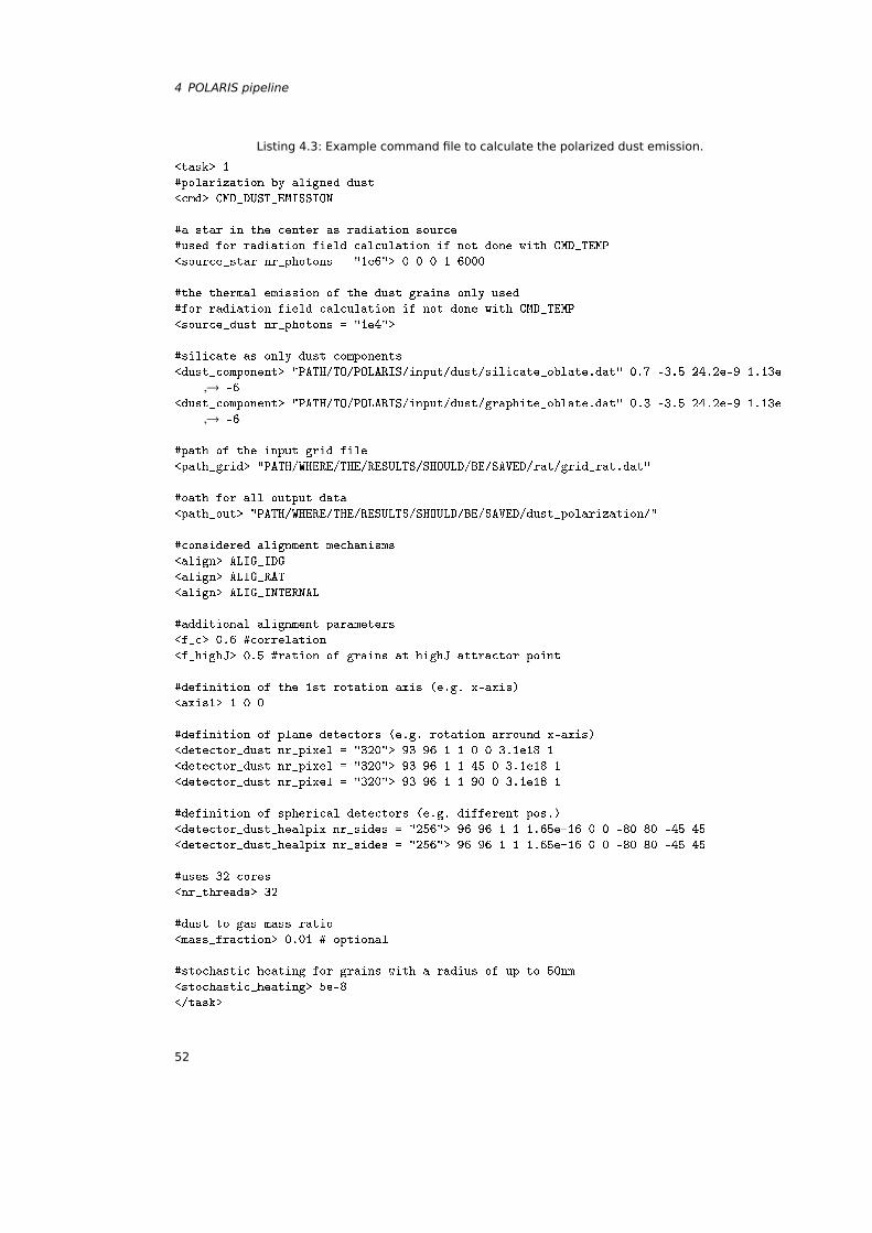
4 POLARIS pipeline
Listing 4.3: Example command file to calculate the polarized dust emission.
<task> 1
#polarization by aligned dust
<cmd> CMD_DUST_EMISSION
#a star in the center as radiation source
#used for radiation field calculation if not done with CMD_TEMP
<source_star nr_photons = "1e6"> 0 0 0 1 6000
#the thermal emission of the dust grains only used
#for radiation field calculation if not done with CMD_TEMP
<source_dust nr_photons = "1e4">
#silicate as only dust components
<dust_component> "PATH/TO/POLARIS/input/dust/silicate_oblate.dat" 0.7 -3.5 24.2e-9 1.13e
→ -6
<dust_component> "PATH/TO/POLARIS/input/dust/graphite_oblate.dat" 0.3 -3.5 24.2e-9 1.13e
→ -6
#path of the input grid file
<path_grid> "PATH/WHERE/THE/RESULTS/SHOULD/BE/SAVED/rat/grid_rat.dat"
#oath for all output data
<path_out> "PATH/WHERE/THE/RESULTS/SHOULD/BE/SAVED/dust_polarization/"
#considered alignment mechanisms
<align> ALIG_IDG
<align> ALIG_RAT
<align> ALIG_INTERNAL
#additional alignment parameters
<f_c> 0.6 #correlation
<f_highJ> 0.5 #ration of grains at highJ attractor point
#definition of the 1st rotation axis (e.g. x-axis)
<axis1> 1 0 0
#definition of plane detectors (e.g. rotation arround x-axis)
<detector_dust nr_pixel = "320"> 93 96 1 1 0 0 3.1e18 1
<detector_dust nr_pixel = "320"> 93 96 1 1 45 0 3.1e18 1
<detector_dust nr_pixel = "320"> 93 96 1 1 90 0 3.1e18 1
#definition of spherical detectors (e.g. different pos.)
<detector_dust_healpix nr_sides = "256"> 96 96 1 1 1.65e+16 0 0 -80 80 -45 45
<detector_dust_healpix nr_sides = "256"> 96 96 1 1 1.65e+16 0 0 -80 80 -45 45
#uses 32 cores
<nr_threads> 32
#dust to gas mass ratio
<mass_fraction> 0.01 # optional
#stochastic heating for grains with a radius of up to 50nm
<stochastic_heating> 5e-8
</task>
52
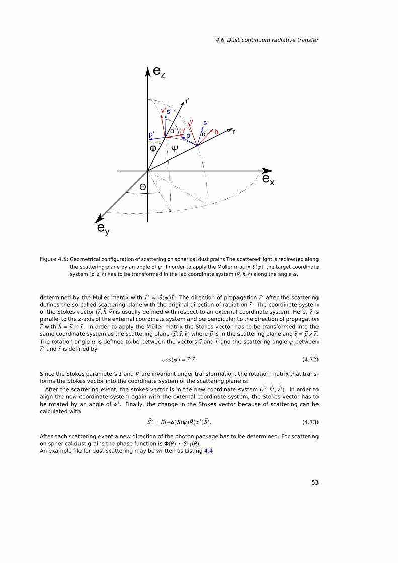
4.6 Dust continuum radiative transfer
ex
ey
ez
v
v'
r
r'
hh's
p
s'
p' α
Ψ
Θ
Φ
α'
Figure 4.5: Geometrical configuration of scattering on spherical dust grains The scattered light is redirected along
the scattering plane by an angle of ψ. In order to apply the Müller matrix S (ψ), the target coordinate
system ( ®p, ®s, ®r ) has to be transformed in the lab coordinate system (®v , ®h, ®r ) along the angle α .
determined by the Müller matrix with ®I ′ ∝ S (ψ) ®I . The direction of propagation ®r ′ after the scatteringdefines the so called scattering plane with the original direction of radiation ®r . The coordinate systemof the Stokes vector (®r , ®h, ®v ) is usually defined with respect to an external coordinate system. Here, ®v isparallel to the z-axis of the external coordinate system and perpendicular to the direction of propagation®r with ®h = ®v × ®r . In order to apply the Müller matrix the Stokes vector has to be transformed into thesame coordinate system as the scattering plane ( ®p, ®s, ®v ) where ®p is in the scattering plane and ®s = ®p × ®r .The rotation angle α is defined to be between the vectors ®s and ®h and the scattering angle ψ between®r ′ and ®r is defined by
cos(ψ) = ®r ′®r . (4.72)
Since the Stokes parameters I andV are invariant under transformation, the rotation matrix that trans-forms the Stokes vector into the coordinate system of the scattering plane is:
After the scattering event, the stokes vector is in the new coordinate system ( ®r ′, ®h ′, ®v ′). In order toalign the new coordinate system again with the external coordinate system, the Stokes vector has tobe rotated by an angle of α ′. Finally, the change in the Stokes vector because of scattering can becalculated with
®S ′ = R (−α)S (ψ)R (α ′) ®S ′. (4.73)
After each scattering event a new direction of the photon package has to be determined. For scatteringon spherical dust grains the phase function is Φ(θ) ∝ S11(θ).An example file for dust scattering may be written as Listing 4.4
53
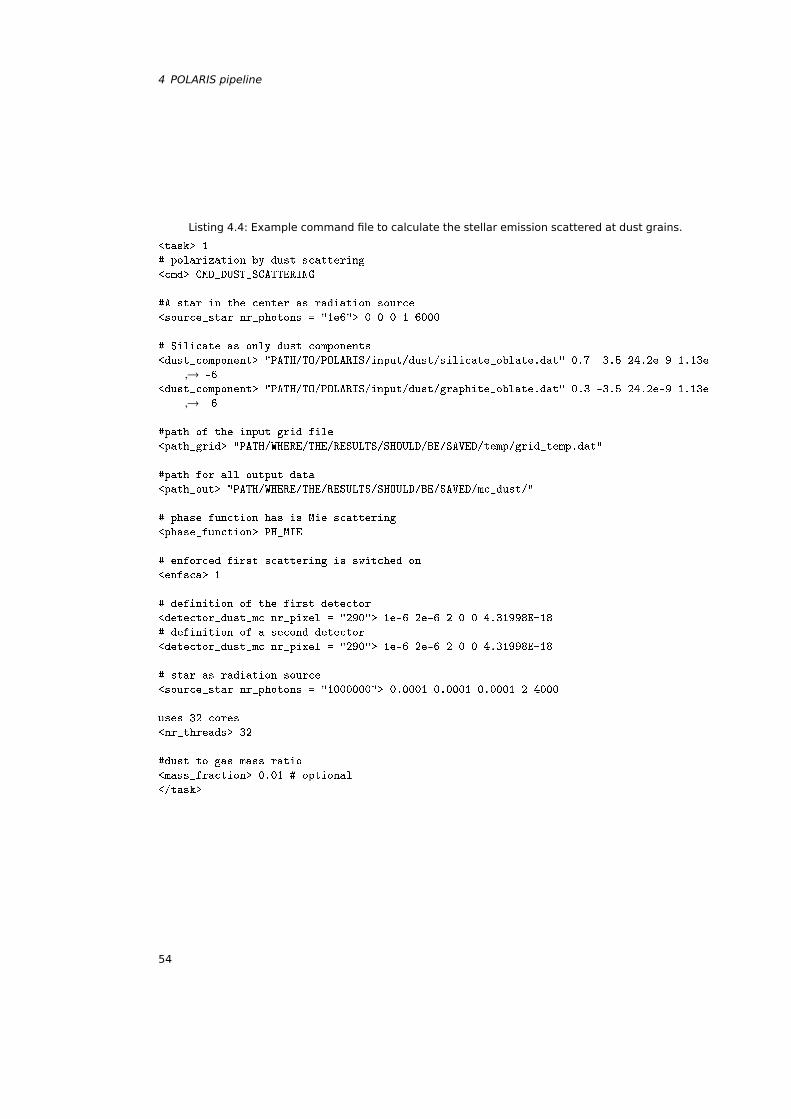
4 POLARIS pipeline
Listing 4.4: Example command file to calculate the stellar emission scattered at dust grains.
<task> 1
# polarization by dust scattering
<cmd> CMD_DUST_SCATTERING
#A star in the center as radiation source
<source_star nr_photons = "1e6"> 0 0 0 1 6000
# Silicate as only dust components
<dust_component> "PATH/TO/POLARIS/input/dust/silicate_oblate.dat" 0.7 -3.5 24.2e-9 1.13e
→ -6
<dust_component> "PATH/TO/POLARIS/input/dust/graphite_oblate.dat" 0.3 -3.5 24.2e-9 1.13e
→ -6
#path of the input grid file
<path_grid> "PATH/WHERE/THE/RESULTS/SHOULD/BE/SAVED/temp/grid_temp.dat"
#path for all output data
<path_out> "PATH/WHERE/THE/RESULTS/SHOULD/BE/SAVED/mc_dust/"
# phase function has is Mie scattering
<phase_function> PH_MIE
# enforced first scattering is switched on
<enfsca> 1
# definition of the first detector
<detector_dust_mc nr_pixel = "290"> 1e-6 2e-6 2 0 0 4.31998E+18
# definition of a second detector
<detector_dust_mc nr_pixel = "290"> 1e-6 2e-6 2 0 0 4.31998E+18
# star as radiation source
<source_star nr_photons = "1000000"> 0.0001 0.0001 0.0001 2 4000
uses 32 cores
<nr_threads> 32
#dust to gas mass ratio
<mass_fraction> 0.01 # optional
</task>
54
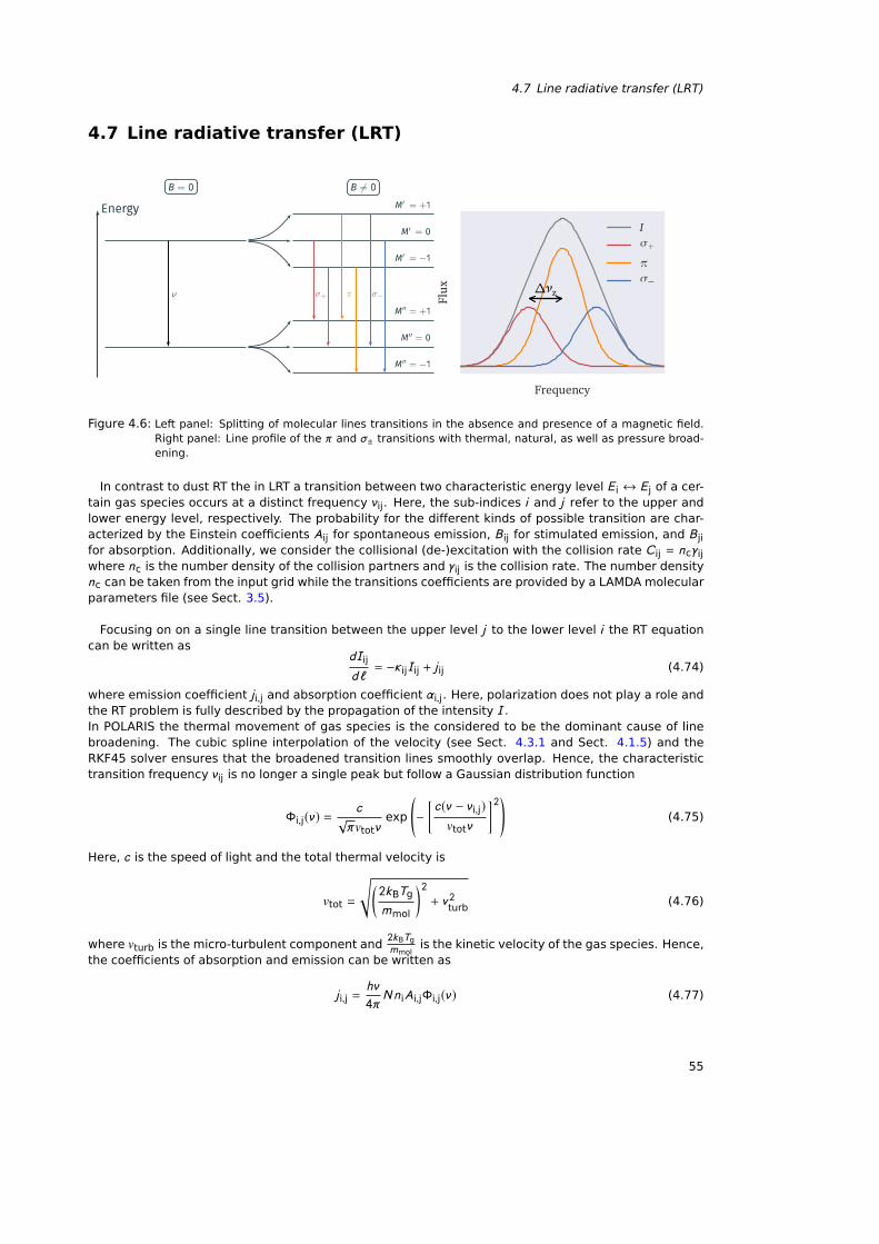
4.7 Line radiative transfer (LRT)
4.7 Line radiative transfer (LRT)
Figure 4.6: Left panel: Splitting of molecular lines transitions in the absence and presence of a magnetic field.Right panel: Line profile of the π and σ± transitions with thermal, natural, as well as pressure broad-ening.
In contrast to dust RT the in LRT a transition between two characteristic energy level Ei ↔ Ej of a cer-tain gas species occurs at a distinct frequency νij. Here, the sub-indices i and j refer to the upper andlower energy level, respectively. The probability for the different kinds of possible transition are char-acterized by the Einstein coefficients Aij for spontaneous emission, Bij for stimulated emission, and Bjifor absorption. Additionally, we consider the collisional (de-)excitation with the collision rate Cij = ncγijwhere nc is the number density of the collision partners and γij is the collision rate. The number densitync can be taken from the input grid while the transitions coefficients are provided by a LAMDA molecularparameters file (see Sect. 3.5).
Focusing on on a single line transition between the upper level j to the lower level i the RT equationcan be written as
dIij
d`= −κijIij + jij (4.74)
where emission coefficient ji,j and absorption coefficient αi,j. Here, polarization does not play a role andthe RT problem is fully described by the propagation of the intensity I .In POLARIS the thermal movement of gas species is the considered to be the dominant cause of linebroadening. The cubic spline interpolation of the velocity (see Sect. 4.3.1 and Sect. 4.1.5) and theRKF45 solver ensures that the broadened transition lines smoothly overlap. Hence, the characteristictransition frequency νij is no longer a single peak but follow a Gaussian distribution function
Φi,j(ν) =c√
πvtotνexp
(−
[c(ν − νi,j)
vtotν
]2)(4.75)
Here, c is the speed of light and the total thermal velocity is
vtot =
√(2kBTg
mmol
)2+ v 2
turb(4.76)
where vturb is the micro-turbulent component and2kBTgmmol
is the kinetic velocity of the gas species. Hence,the coefficients of absorption and emission can be written as
ji,j =hν
4πNn iAi,jΦi,j(ν) (4.77)
55
4 POLARIS pipeline
and
αi,j =hν
4πN
(n jBj,i − n iBi,j
)Φi,j(ν) (4.78)
respectively, where n i is the number of electrons on the i -th level. Balancing the full RT equation withthe contributions of collisional excitation and de-excitation and the mean intensity
Ji,j =1
4π
∫ ∫IνΦi,j(ν)dΩdν (4.79)
gives ∑i>j
[n iAij +
(n iBij − n jBji
)Ji,j
] −∑i<j
[n jAji +
(n jBji − n iBij
) ]+
∑i
(n iCij + n jCji
)(4.80)
This system of equations is solved with the help of Gaussian elimination.The command to define all the parameters for a gas species to be observed is
<gas_species> "path" POP a
Here, the path gives the LAMDA gas species parameters file, a is the abundance with respect to thetotal gas density, and POP stands for the index for the different implemented methods for calculatingthe level populations (1: LTE, 2: FEP, 3: LVG; see Sect. 4.7.1).
Example:
<gas_species> "/PATH/TO/POLARIS/input/gas/co.dat" 2 1e-7
The defined gas species can then selected by a line detector with an ID coinciding with the order ofappearance in the command file (see Sect. 4.5 for defining the line detector).
4.7.1 Level population approximations
In order to perform LRT simulations one needs to calculate the level populations. Several numericalmethods are known to calculate level populations considering different local conditions.
Local thermodynamic equilibrium (LTE)
For this approximation it is assumed that the different level populations are thermalized meaning thatexcitation temperature Texc and kinetic gas temperature Tg are equal:
Tg = Texc =hνi,j
kB
[ln
(gin j
gjn i
)]−1(4.81)
Here, n i id the number of electrons in the i-th level of the gas species, gi is the corresponding statisticalweight and νi,j is the frequency characteristic for that transition. Hence, the level populations follow theBoltzmann distribution with
n i
n j=gi
gjexp
(hνi,j
kBTg
)(4.82)
This approximation can be adequate when the optical depth of a transition is so high that the collisionaland radiative excitations and de-excitation, respectively, are approximately in equilibrium. In order toapply LTE in LRT simulations the flag POP_LTE need to be added in the command line defining the gasspecies.
Full escape probability (FEP)
FEP assumes that any newly created photon can escape the grid without any further interactions. Thelevel populations can then be calculated by simply applying an external radiation field Ji,j = Jext to Eq.4.80.Hence, the FEP method applies for low molecular abundances. Considering FEP in a POLARIS run theflag POP_LTE needs to be added.
56
4.7 Line radiative transfer (LRT)
Large velocity gradient (LVG)
This approximation assumes that a photon can easily escape from the grid because of a large gradientin the velocities of neighboring regions. For the LVG the mean intensity is due to the local transition andan external radiation field
Ji,j = (1 − β )Si,j + β Jext (4.83)
Here, β is the probability for the photons to escape from the grid and is given by
β =1 − exp(τi,j)
τi,j(4.84)
where as
Si,j =ji,j
αi,j=
n iAi,j
n jBji − n iBij(4.85)
is the source function of the transition. For this approximation the required optical depth τi,j can becalculated as
τij =c3ngAij
8πν3ij|dv/d l |
(gi
gjn j − n i
)(4.86)
given a large enough velocity gradient |dv/d` |. This approximation can be applied when the variationsin velocity are larger than the local thermal and micro-turbulent velocities. Using LVG requires the tagPOP_LVG. At the beginning of each LRT run POLARIS pre-calculates the level population for each cellof the grid. The methods of LTE and FEP require little computational efforts. In contrast, LVG is moretime consuming for a large number of cells since its need to solve Eq. 4.80 iteratively. However, thecalculation of level populations is parallelized in POLARIS.
HINTS:
• If the abundance a is negative, this number means the abundance is taken from the input grid.
An exemplary LRT command file in POLARIS may look like as shown in Listing 4.5.
4.7.2 LRT with Zeeman effect
In POLARIS, the implementation of LRT including Zeeman splitting is based on the work of Larsson et al.(2014). The energy levels of a gas species can split into separate distinct sub-level when a gas speciesis exposed by an external magnetic field (see Sect. 4.6). This splitting of spectral lines is referred asto Zeeman effect. Here, the degeneracy of the sub-level is given by 2J + 1 and the magnetic quantumnumber can get the values of
mJ = [−J ,−J + 1, ..., J − 1, J ] . (4.87)
The energy of any transition is given by:
∆E = −(®µ ®B
)= gJµ0∆mJB . (4.88)
Here, B is the magnetic field strength, µ0 is the Bohr magneton . The Landè factor gJ is defined as afraction of quantum numbers and a gas species specific constant gs by
gJ = gsJ (J + 1) + S (S + 1) + N (N + 1)
2J (J + 1) . (4.89)
The difference in energy between different sub-level allows to calculate the characteristic frequency ofeach transition
ν0 =Bµ0h
(gJ′mJ′ − gJ′′mJ′′
)(4.90)
where ′ and ′′ indicate the upper and lower sub-level, respectively.
57
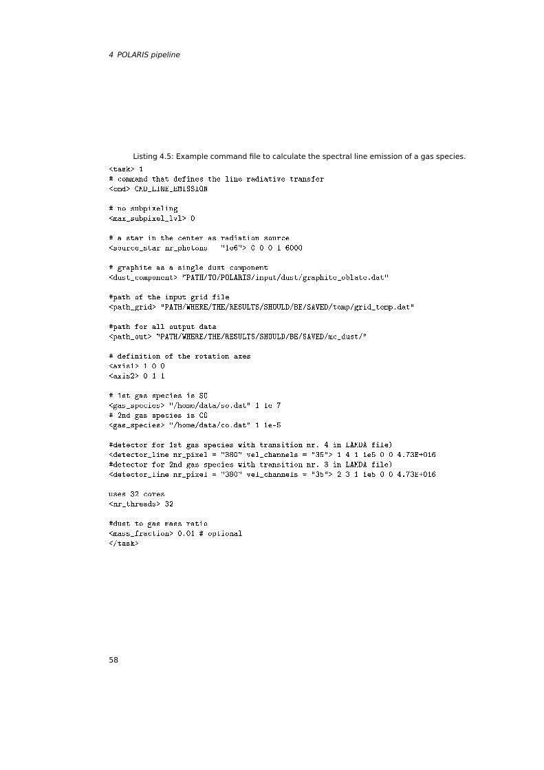
4 POLARIS pipeline
Listing 4.5: Example command file to calculate the spectral line emission of a gas species.
<task> 1
# command that defines the line radiative transfer
<cmd> CMD_LINE_EMISSION
# no subpixeling
<max_subpixel_lvl> 0
# a star in the center as radiation source
<source_star nr_photons = "1e6"> 0 0 0 1 6000
# graphite as a single dust component
<dust_component> "PATH/TO/POLARIS/input/dust/graphite_oblate.dat"
#path of the input grid file
<path_grid> "PATH/WHERE/THE/RESULTS/SHOULD/BE/SAVED/temp/grid_temp.dat"
#path for all output data
<path_out> "PATH/WHERE/THE/RESULTS/SHOULD/BE/SAVED/mc_dust/"
# definition of the rotation axes
<axis1> 1 0 0
<axis2> 0 1 1
# 1st gas species is SO
<gas_species> "/home/data/so.dat" 1 1e-7
# 2nd gas species is CO
<gas_species> "/home/data/co.dat" 1 1e-5
#detector for 1st gas species with transition nr. 4 in LAMDA file)
<detector_line nr_pixel = "380" vel_channels = "35"> 1 4 1 1e5 0 0 4.73E+016
#detector for 2nd gas species with transition nr. 3 in LAMDA file)
<detector_line nr_pixel = "380" vel_channels = "35"> 2 3 1 1e5 0 0 4.73E+016
uses 32 cores
<nr_threads> 32
#dust to gas mass ratio
<mass_fraction> 0.01 # optional
</task>
58
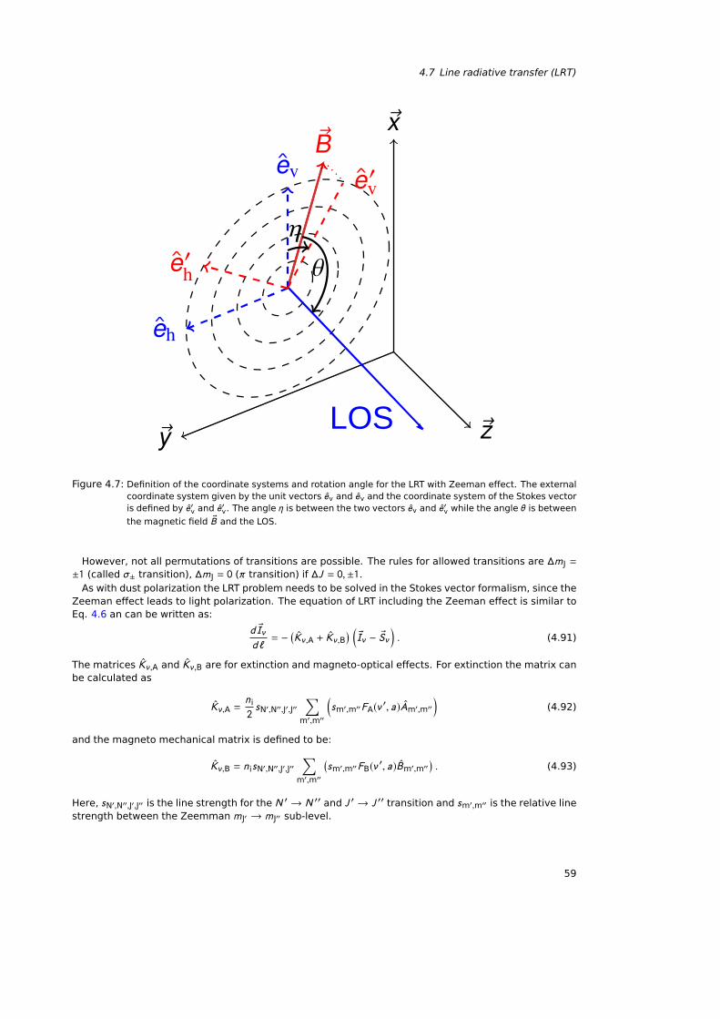
4.7 Line radiative transfer (LRT)
LOS
Figure 4.7: Definition of the coordinate systems and rotation angle for the LRT with Zeeman effect. The externalcoordinate system given by the unit vectors ev and ev and the coordinate system of the Stokes vectoris defined by e′v and e′v. The angle η is between the two vectors ev and e′v while the angle θ is between
the magnetic field ®B and the LOS.
However, not all permutations of transitions are possible. The rules for allowed transitions are ∆mJ =±1 (called σ± transition), ∆mJ = 0 (π transition) if ∆J = 0,±1.
As with dust polarization the LRT problem needs to be solved in the Stokes vector formalism, since theZeeman effect leads to light polarization. The equation of LRT including the Zeeman effect is similar toEq. 4.6 an can be written as:
d ®Iνd`
= − (Kν,A + Kν,B
) (®Iν − ®Sν
). (4.91)
The matrices Kν,A and Kν,B are for extinction and magneto-optical effects. For extinction the matrix canbe calculated as
Kν,A =n i
2sN′,N′′,J′,J′′
∑m′,m′′
(sm′,m′′FA(ν′, a)Am′,m′′
)(4.92)
and the magneto mechanical matrix is defined to be:
Kν,B = n isN′,N′′,J′,J′′∑
m′,m′′
(sm′,m′′FB(ν′, a)Bm′,m′′
). (4.93)
Here, sN′,N′′,J′,J′′ is the line strength for the N ′ → N ′′ and J ′ → J ′′ transition and sm′,m′′ is the relative linestrength between the Zeemman mJ′ → mJ′′ sub-level.
59
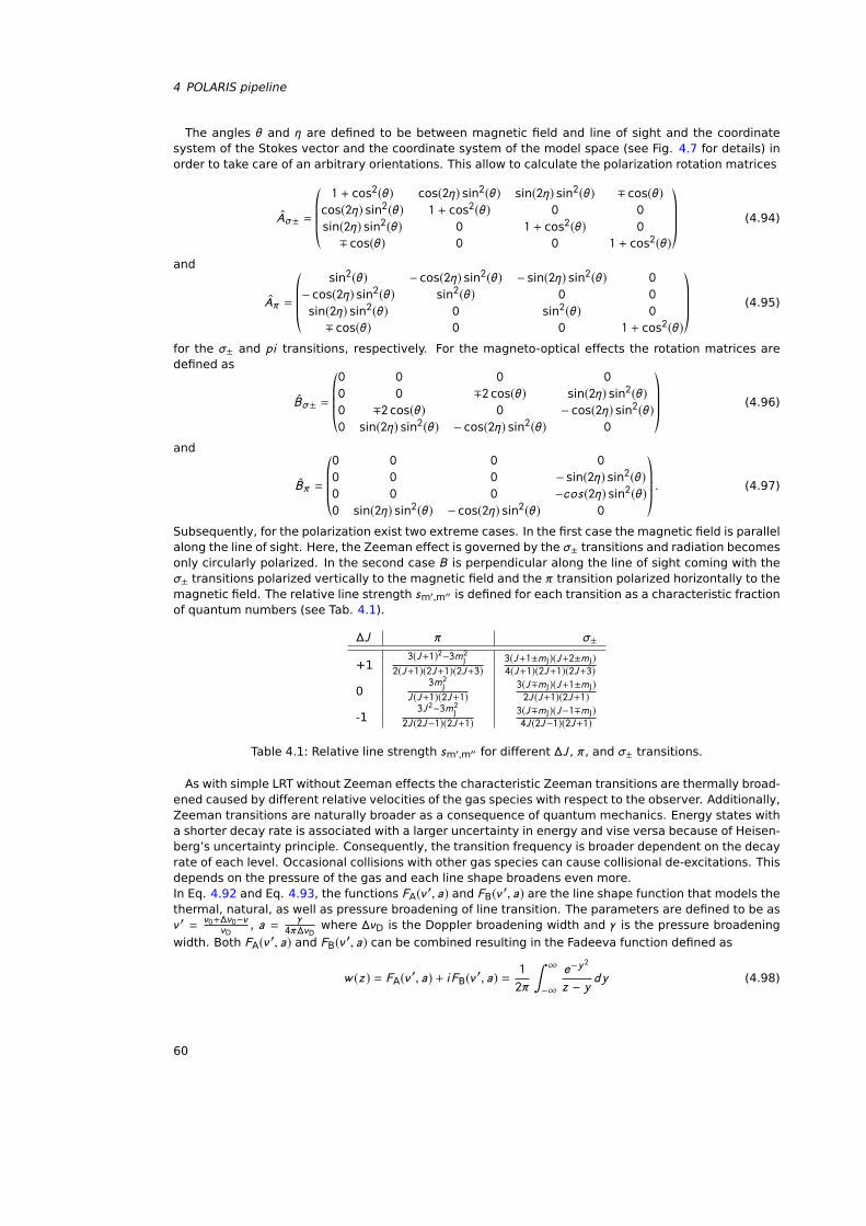
4 POLARIS pipeline
The angles θ and η are defined to be between magnetic field and line of sight and the coordinatesystem of the Stokes vector and the coordinate system of the model space (see Fig. 4.7 for details) inorder to take care of an arbitrary orientations. This allow to calculate the polarization rotation matrices
Aσ± =©«1 + cos2(θ) cos(2η) sin2(θ) sin(2η) sin2(θ) ∓ cos(θ)
cos(2η) sin2(θ) 1 + cos2(θ) 0 0
sin(2η) sin2(θ) 0 1 + cos2(θ) 0
∓ cos(θ) 0 0 1 + cos2(θ)
ª®®®¬ (4.94)
and
Aπ =©«
sin2(θ) − cos(2η) sin2(θ) − sin(2η) sin2(θ) 0
− cos(2η) sin2(θ) sin2(θ) 0 0
sin(2η) sin2(θ) 0 sin2(θ) 0
∓ cos(θ) 0 0 1 + cos2(θ)
ª®®®¬ (4.95)
for the σ± and pi transitions, respectively. For the magneto-optical effects the rotation matrices aredefined as
Bσ± =©«0 0 0 0
0 0 ∓2 cos(θ) sin(2η) sin2(θ)0 ∓2 cos(θ) 0 − cos(2η) sin2(θ)0 sin(2η) sin2(θ) − cos(2η) sin2(θ) 0
ª®®®¬ (4.96)
and
Bπ =©«0 0 0 0
0 0 0 − sin(2η) sin2(θ)0 0 0 −cos(2η) sin2(θ)0 sin(2η) sin2(θ) − cos(2η) sin2(θ) 0
ª®®®¬ . (4.97)
Subsequently, for the polarization exist two extreme cases. In the first case the magnetic field is parallelalong the line of sight. Here, the Zeeman effect is governed by the σ± transitions and radiation becomesonly circularly polarized. In the second case B is perpendicular along the line of sight coming with theσ± transitions polarized vertically to the magnetic field and the π transition polarized horizontally to themagnetic field. The relative line strength sm′,m′′ is defined for each transition as a characteristic fractionof quantum numbers (see Tab. 4.1).
∆J π σ±
+13(J+1)2−3m2
J
2(J+1)(2J+1)(2J+3)3(J+1±mJ)(J+2±m J)4(J+1)(2J+1)(2J+3)
03m2
J
J (J+1)(2J+1)3(J∓mJ)(J+1±m J)2J (J+1)(2J+1)
-13J 2−3m2
J
2J (2J−1)(2J+1)3(J∓mJ)(J−1∓m J)4J (2J−1)(2J+1)
Table 4.1: Relative line strength sm′,m′′ for different ∆J , π, and σ± transitions.
As with simple LRT without Zeeman effects the characteristic Zeeman transitions are thermally broad-ened caused by different relative velocities of the gas species with respect to the observer. Additionally,Zeeman transitions are naturally broader as a consequence of quantum mechanics. Energy states witha shorter decay rate is associated with a larger uncertainty in energy and vise versa because of Heisen-berg’s uncertainty principle. Consequently, the transition frequency is broader dependent on the decayrate of each level. Occasional collisions with other gas species can cause collisional de-excitations. Thisdepends on the pressure of the gas and each line shape broadens even more.In Eq. 4.92 and Eq. 4.93, the functions FA(ν′, a) and FB(ν′, a) are the line shape function that models thethermal, natural, as well as pressure broadening of line transition. The parameters are defined to be asν′ = ν0+∆ν0−ν
νD, a = γ
4π∆νDwhere ∆νD is the Doppler broadening width and γ is the pressure broadening
width. Both FA(ν′, a) and FB(ν′, a) can be combined resulting in the Fadeeva function defined as
w (z ) = FA(ν′, a) + i FB(ν′, a) =1
2π
∫ ∞−∞
e−y 2
z − y dy (4.98)
60
4.8 Synchrotron RT
with z = ν′ + i a. In the POLARIS code the solution to this problem is solved with the help of the C++
Fadeeva package 1. The Fadeeva function may in principle also be applied for simple LRT. However, theLAMDA files do not provide the necessary paramters to do so. This may be solved in a future versionof POLARIS. For Zeeman splitting there is a correlation between the Stokes V parameter and the firstvelocity derivative dI /dv
V =dI
dν∆ν cos(θ) (4.99)
where∆ν =
µ0h
(gJ′mJ′ − gJ′′mJ′′
). (4.100)
Bohr magneton µ0 and the Planck constant h are known and the quantities gJ′ and mJ′ can be pre-calculated for each gas species. Hence, the line of sight magnetic field strength B cos(θ) can be calcu-lated with POLARIS by simulating the Stokes I andV parameters and the subsequent fitting of dIdν ontoV .In POLARIS a LRT run including the Zeeman effect is almost identical to a simple RT as presented in theprevious section. However, simulating the Zeeman effect requires the quantities of the Landè factor(see Eq. 4.89) and the relative line strength (see Tab. 4.1). The values for these quantities need to bedelivered in an extra file (see Sect. 3.5.2) corresponding to the Leiden molecular file. Instead of a singlepath for the LAMDA file on need to add a second path to the corresponding Zeeman file:
<gas_species> "path" POP a "path Zeeman"
Example:
<gas_species> "/PATH/TO/POLARIS/input/gas/oh.dat" 1 1e-5 "/PATH/TO/POLARIS/input/gas/
→ oh_zeeman.dat"
An exemplary LRT command file in POLARIS with Zeeman splitting may look like as shown in Listing4.6.
4.8 Synchrotron RT
When a moving electron is forced on a curved path or an orbit it emits radiation. In particular freeelectrons in the ISM gyrate around the magnetic field lines. This leads to polarized radiation as well asrotation of the polarization plane of background radiation (Faraday effect).For a complete synchrotron RT, one needs to consider two different species of electrons: cosmic ray (CR)electrons and thermalized relativistic electrons. Synchrotron intensity as well as linear and circular po-larization emerges mostly from CR electrons where as thermal electrons dominate Faraday rotation (FR)and Faraday conversion (FC). The RT problem is identical to that of Eq. 4.6. The synchrotron requiredcoefficients can be calculated by integrals over modified Bessel functions. However, due to performancereasons, the implementation in POLARIS follows the approach of applying fitting functions approximatingthe exact integral solutions. These fitting functions provide high accuracy solutions for typical ISM-likeconditions. The implementation in POLARIS is based on the functions presented in Pandya et al. (2016)and Dexter (2016).
4.8.1 CR electrons
The energy of CR electrons follow a power-law distribution
NCR(γ) =nCRγ
p (p − 1)(γp−1min− γp−1max
)if γmin < γ < γmax
0 otherwise(4.101)
1http://ab-initio.mit.edu/wiki/index.php/Faddeeva_Package, Copyright c© 2012 Massachusetts Institute of Technol-ogy
61
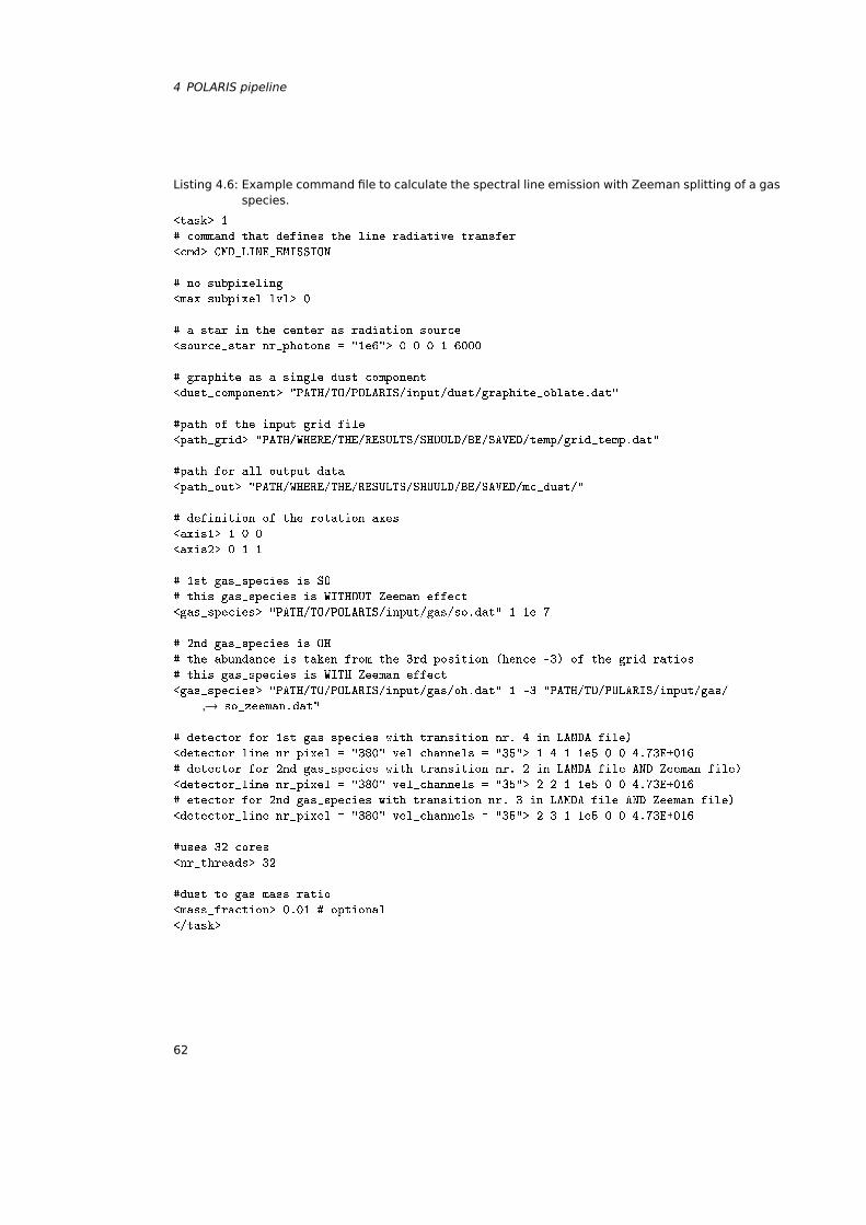
4 POLARIS pipeline
Listing 4.6: Example command file to calculate the spectral line emission with Zeeman splitting of a gasspecies.
<task> 1
# command that defines the line radiative transfer
<cmd> CMD_LINE_EMISSION
# no subpixeling
<max_subpixel_lvl> 0
# a star in the center as radiation source
<source_star nr_photons = "1e6"> 0 0 0 1 6000
# graphite as a single dust component
<dust_component> "PATH/TO/POLARIS/input/dust/graphite_oblate.dat"
#path of the input grid file
<path_grid> "PATH/WHERE/THE/RESULTS/SHOULD/BE/SAVED/temp/grid_temp.dat"
#path for all output data
<path_out> "PATH/WHERE/THE/RESULTS/SHOULD/BE/SAVED/mc_dust/"
# definition of the rotation axes
<axis1> 1 0 0
<axis2> 0 1 1
# 1st gas_species is SO
# this gas_species is WITHOUT Zeeman effect
<gas_species> "PATH/TO/POLARIS/input/gas/so.dat" 1 1e-7
# 2nd gas_species is OH
# the abundance is taken from the 3rd position (hence -3) of the grid ratios
# this gas_species is WITH Zeeman effect
<gas_species> "PATH/TO/POLARIS/input/gas/oh.dat" 1 -3 "PATH/TO/POLARIS/input/gas/
→ so_zeeman.dat"
# detector for 1st gas species with transition nr. 4 in LAMDA file)
<detector_line nr_pixel = "380" vel_channels = "35"> 1 4 1 1e5 0 0 4.73E+016
# detector for 2nd gas_species with transition nr. 2 in LAMDA file AND Zeeman file)
<detector_line nr_pixel = "380" vel_channels = "35"> 2 2 1 1e5 0 0 4.73E+016
# etector for 2nd gas_species with transition nr. 3 in LAMDA file AND Zeeman file)
<detector_line nr_pixel = "380" vel_channels = "35"> 2 3 1 1e5 0 0 4.73E+016
#uses 32 cores
<nr_threads> 32
#dust to gas mass ratio
<mass_fraction> 0.01 # optional
</task>
62
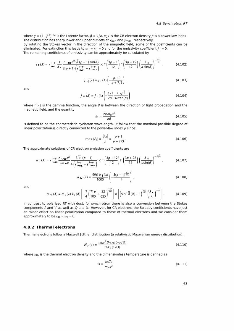
4.8 Synchrotron RT
where γ = (1−β2)1/2 is the Lorentz factor, β = v/c, nCR is the CR electron density p is a power-law index.The distribution has sharp lower and upper cut-offs at γmin and γmax, respectively.By rotating the Stokes vector in the direction of the magnetic field, some of the coefficients can beeliminated. For extinction this leads to αU = κU = 0 and for the emissivity coefficient jU = 0.The remaining coefficients of emissivity can be approximately be calculated by
j I (λ) = γ1−pmin1
λ c
n CRe23
p2 (p − 1) sin(ϑ)
2(p + 1)(γ1−pmin− γ1−pmax
) × Γ (3p − 112
)Γ
(3p + 19
12
) (λ c
λ sin(ϑ)
)− p−12, (4.102)
j Q (λ) = j I (λ)(− p + 1
p + 7/3
), (4.103)
and
j V (λ) = j I (λ)(−171250
λ cp12
3λ tan(ϑ)
)(4.104)
where Γ(x ) is the gamma function, the angle θ is between the direction of light propagation and themagnetic field, and the quantity
λc =2πmec
2
eB(4.105)
is defined to be the characteristic cyclotron wavelength. It follow that the maximal possible degree oflinear polarization is directly connected to the power-law index p since:
max (Pl) =jQjI
=p + 1
p + 7/3 . (4.106)
The approximate solutions of CR electron emission coefficients are
α I (λ) = γ1−pminn CRe
2
νm ec
3p+12 (p − 1)
4(γ1−pmin− γ1−pmax
) × Γ (3p + 12
12
)Γ
(3p + 22
12
) (λ c
λ sin(ϑ)
)− p+22, (4.107)
α Q (λ) =996 α I (λ)1000
(−3(p − 1)
43500
4
), (4.108)
and
α V (λ) = α I (λ) kV (ϑ)[−74
(71p
100+22
625
) 197500
]×
[(sin−
4825 (ϑ) − 1
) 64125
(λ c
λ
)− 12 ]. (4.109)
In contrast to polarized RT with dust, for synchrotron there is also a conversion between the Stokescomponents I and V as well as Q and U . However, for CR electrons the Faraday coefficients have justan minor effect on linear polarization compared to those of thermal electrons and we consider themapproximately to be κQ = κV = 0.
4.8.2 Thermal electrons
Thermal electrons follow a Maxwell Jüttner distribution (a relativistic Maxwellian energy distribution):
Nth(γ) =nthγ
2β exp (−γ/Θ)ΘK2 (1/Θ)
(4.110)
where nth is the thermal electron density and the dimensionless temperature is defined as
Θ =kBTe
mec2(4.111)
63
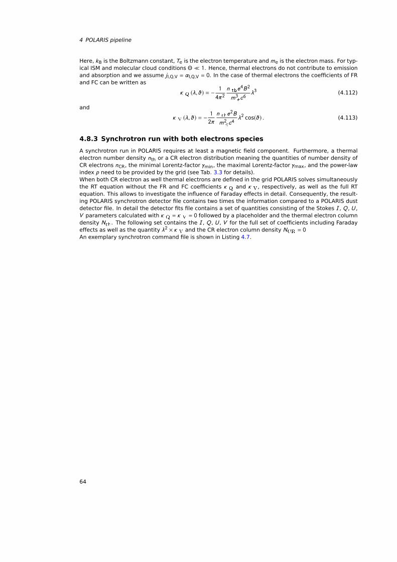
4 POLARIS pipeline
Here, kB is the Boltzmann constant,Te is the electron temperature and me is the electron mass. For typ-ical ISM and molecular cloud conditions Θ 1. Hence, thermal electrons do not contribute to emissionand absorption and we assume jI,Q,V = αI,Q,V = 0. In the case of thermal electrons the coefficients of FRand FC can be written as
κ Q (λ, ϑ) = −1
4π2n the
4B2
m3ec6λ3 (4.112)
and
κ V (λ, ϑ) = −1
2π
n the2B
m2ec4λ2 cos(ϑ) . (4.113)
4.8.3 Synchrotron run with both electrons species
A synchrotron run in POLARIS requires at least a magnetic field component. Furthermore, a thermalelectron number density nth or a CR electron distribution meaning the quantities of number density ofCR electrons nCR, the minimal Lorentz-factor γmin, the maximal Lorentz-factor γmax, and the power-lawindex p need to be provided by the grid (see Tab. 3.3 for details).When both CR electron as well thermal electrons are defined in the grid POLARIS solves simultaneouslythe RT equation without the FR and FC coefficients κ Q and κ V, respectively, as well as the full RTequation. This allows to investigate the influence of Faraday effects in detail. Consequently, the result-ing POLARIS synchrotron detector file contains two times the information compared to a POLARIS dustdetector file. In detail the detector fits file contains a set of quantities consisting of the Stokes I , Q , U ,V parameters calculated with κ Q = κ V = 0 followed by a placeholder and the thermal electron columndensity Nth. The following set contains the I , Q , U , V for the full set of coefficients including Faradayeffects as well as the quantity λ2 × κ V and the CR electron column density NCR = 0An exemplary synchrotron command file is shown in Listing 4.7.
64
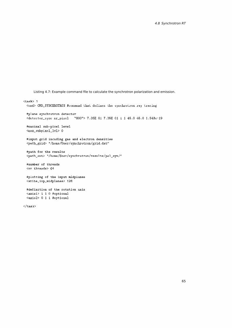
4.8 Synchrotron RT
Listing 4.7: Example command file to calculate the synchrotron polarization and emission.
<task> 1
<cmd> CMD_SYNCHROTRON #command that defines the synchrotron ray-tracing
#plane synchrotron detector
<detector_sync nr_pixel = "800"> 7.35E-01 7.35E-01 1 1 45.0 45.0 1.543e+19
#maximal sub-pixel level
<max_subpixel_lvl> 0
#input grid incuding gas and electron densities
<path_grid> "/home/User/synchrotron/grid.dat"
#path for the results
<path_out> "/home/User/synchrotron/results/pol_syn/"
#number of threads
<nr_threads> 64
#plotting of the input midplanes
<write_inp_midplanes> 128
#definition of the rotation axis
<axis1> 1 1 0 #optional
<axis2> 0 1 1 #optional
</task>
65

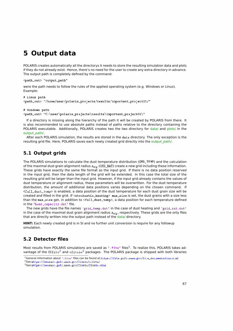
5 Output data
POLARIS creates automatically all the directorys it needs to store the resulting simulation data and plotsif they do not already exist. Hence, there’s no need for the user to create any extra directory in advance.The output path is completely defined by the command:
<path_out> "output_path"
were the path needs to follow the rules of the applied operating system (e.g. Windows or Linux).Example:
# Linux path
<path_out> "/home/user/polaris_projects/results/important_project01/"
# Windows path
<path_out> "C:\user\polaris_projects\results\important_project01\"
If a directory is missing along the hierarchy of the path it will be created by POLARIS from there. Itis also recommended to use absolute paths instead of paths relative to the directory containing thePOLARIS executable. Additionally, POLARIS creates two the two directory for data/ and plots/ in theoutput_path/.
After each POLARIS simulation, the results are stored in the data directory. The only exception is theresulting grid file. Here, POLARIS saves each newly created grid directly into the output_path/.
5.1 Output grids
The POLARIS simulations to calculate the dust temperature distribution (CMD_TEMP) and the calculationof the maximal dust grain alignment radius aal g (CMD_RAT) create a new grid including these information.These grids have exactly the same file format as the input grid. If there is no data position reservedin the input grid, then the data length of the grid will be extended. In this case the total size of theresulting grid will be larger than the input grid. However, if the input grid already contains the values ofdust temperature or alignment radius, these parameters will be overwritten. For the dust temperaturedistribution, the amount of additional data positions varies depending on the chosen command. If<full_dust_temp> is enabled, a data position of the dust temperature for each dust grain size will becreated and filled in the grid. If <stochastic_heating> max_size is set, the dust grains with a size lessthan the max_size get, in addition to <full_dust_temp>, a data position for each temperature definedin the 'heat_capacity.dat' file.
The new grids have the file names 'grid_temp.dat' in the case of dust heating and 'grid_rat.dat'
in the case of the maximal dust grain alignment radius aal g , respectively. These grids are the only filesthat are directly written into the output path instead of the data/ directory.
HINT: Each newly created grid is in SI and no further unit conversion is require for any followupsimulation.
5.2 Detector files
Most results from POLARIS simulations are saved as '.fits' files1. To realize this, POLARIS takes ad-vantage of the CCfits2 and cfitsio3 packages. The POLARIS package is shipped with both libraries
1General information about '.fits' files can be found at https://fits.gsfc.nasa.gov/fits_documentation.html2See https://heasarc.gsfc.nasa.gov/fitsio/ccfits/3See https://heasarc.gsfc.nasa.gov/fitsio/fitsio.html
67
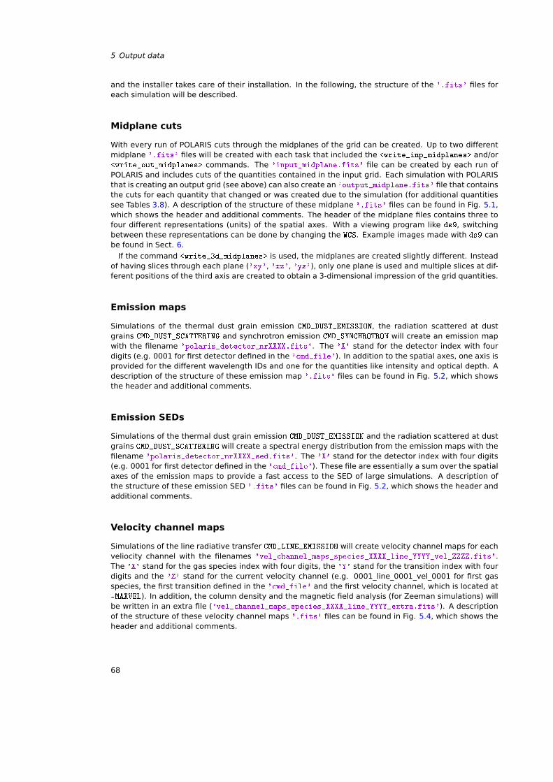
5 Output data
and the installer takes care of their installation. In the following, the structure of the '.fits' files foreach simulation will be described.
Midplane cuts
With every run of POLARIS cuts through the midplanes of the grid can be created. Up to two differentmidplane '.fits' files will be created with each task that included the <write_inp_midplanes> and/or<write_out_midplanes> commands. The 'input_midplane.fits' file can be created by each run ofPOLARIS and includes cuts of the quantities contained in the input grid. Each simulation with POLARISthat is creating an output grid (see above) can also create an 'output_midplane.fits' file that containsthe cuts for each quantity that changed or was created due to the simulation (for additional quantitiessee Tables 3.8). A description of the structure of these midplane '.fits' files can be found in Fig. 5.1,which shows the header and additional comments. The header of the midplane files contains three tofour different representations (units) of the spatial axes. With a viewing program like ds9, switchingbetween these representations can be done by changing the WCS. Example images made with ds9 canbe found in Sect. 6.
If the command <write_3d_midplanes> is used, the midplanes are created slightly different. Insteadof having slices through each plane ('xy', 'xz', 'yz'), only one plane is used and multiple slices at dif-ferent positions of the third axis are created to obtain a 3-dimensional impression of the grid quantities.
Emission maps
Simulations of the thermal dust grain emission CMD_DUST_EMISSION, the radiation scattered at dustgrains CMD_DUST_SCATTERING and synchrotron emission CMD_SYNCHROTRON will create an emission mapwith the filename 'polaris_detector_nrXXXX.fits'. The 'X' stand for the detector index with fourdigits (e.g. 0001 for first detector defined in the 'cmd_file'). In addition to the spatial axes, one axis isprovided for the different wavelength IDs and one for the quantities like intensity and optical depth. Adescription of the structure of these emission map '.fits' files can be found in Fig. 5.2, which showsthe header and additional comments.
Emission SEDs
Simulations of the thermal dust grain emission CMD_DUST_EMISSION and the radiation scattered at dustgrains CMD_DUST_SCATTERING will create a spectral energy distribution from the emission maps with thefilename 'polaris_detector_nrXXXX_sed.fits'. The 'X' stand for the detector index with four digits(e.g. 0001 for first detector defined in the 'cmd_file'). These file are essentially a sum over the spatialaxes of the emission maps to provide a fast access to the SED of large simulations. A description ofthe structure of these emission SED '.fits' files can be found in Fig. 5.2, which shows the header andadditional comments.
Velocity channel maps
Simulations of the line radiative transfer CMD_LINE_EMISSION will create velocity channel maps for eachveliocity channel with the filenames 'vel_channel_maps_species_XXXX_line_YYYY_vel_ZZZZ.fits'.The 'X' stand for the gas species index with four digits, the 'Y' stand for the transition index with fourdigits and the 'Z' stand for the current velocity channel (e.g. 0001_line_0001_vel_0001 for first gasspecies, the first transition defined in the 'cmd_file' and the first velocity channel, which is located at-MAXVEL). In addition, the column density and the magnetic field analysis (for Zeeman simulations) willbe written in an extra file ('vel_channel_maps_species_XXXX_line_YYYY_extra.fits'). A descriptionof the structure of these velocity channel maps '.fits' files can be found in Fig. 5.4, which shows theheader and additional comments.
68
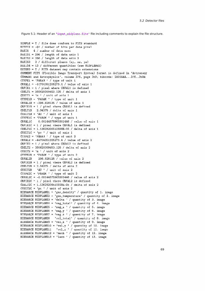
5.2 Detector files
Figure 5.1: Header of an 'input_midplane.fits' file including comments to explain the file structure.
SIMPLE = T / file does conform to FITS standard
BITPIX = -64 / number of bits per data pixel
NAXIS = 4 / number of data axes
NAXIS1 = 256 / length of data axis 1
NAXIS2 = 256 / length of data axis 2
NAXIS3 = 3 / different planes (xy, xz, yz)
NAXIS4 = 13 / different quantities (see MIDPLANEX)
EXTEND = T / FITS dataset may contain extensions
COMMENT FITS (Flexible Image Transport System) format is defined in 'Astronomy
COMMENT and Astrophysics', volume 376, page 359; bibcode: 2001A&A...376..359H
CTYPE1 = 'PARAM ' / type of unit 1
CRVAL1 = -44704051205273.4 / value of axis 1
CRPIX1 = 1 / pixel where CRVAL1 is defined
CDELT1 = 350620009453.125 / delta of axis 1
CUNIT1 = 'm ' / unit of axis 1
CTYPE1B = 'PARAM ' / type of unit 1
CRVAL1B = -298.828125 / value of axis 1
CRPIX1B = 1 / pixel where CRVAL1 is defined
CDELT1B = 2.34375 / delta of axis 1
CUNIT1B = 'AU ' / unit of axis 1
CTYPE1C = 'PARAM ' / type of unit 1
CRVAL1C = -0.00144875963301446 / value of axis 1
CRPIX1C = 1 / pixel where CRVAL1 is defined
CDELT1C = 1.13628206510938E-05 / delta of axis 1
CUNIT1C = 'pc ' / unit of axis 1
CTYPE2 = 'PARAM ' / type of unit 2
CRVAL2 = -44704051205273.4 / value of axis 2
CRPIX2 = 1 / pixel where CRVAL2 is defined
CDELT2 = 350620009453.125 / delta of axis 2
CUNIT2 = 'm ' / unit of axis 2
CTYPE2B = 'PARAM ' / type of unit 2
CRVAL2B = -298.828125 / value of axis 2
CRPIX2B = 1 / pixel where CRVAL2 is defined
CDELT2B = 2.34375 / delta of axis 2
CUNIT2B = 'AU ' / unit of axis 2
CTYPE2C = 'PARAM ' / type of unit 2
CRVAL2C = -0.00144875963301446 / value of axis 2
CRPIX2C = 1 / pixel where CRVAL2 is defined
CDELT2C = 1.13628206510938E-05 / delta of axis 2
CUNIT2C = 'pc ' / unit of axis 2
HIERARCH MIDPLANE1 = 'gas_density' / quantity of 1. image
HIERARCH MIDPLANE2 = 'gas_temperature' / quantity of 2. image
HIERARCH MIDPLANE3 = 'delta ' / quantity of 3. image
HIERARCH MIDPLANE4 = 'mag_total' / quantity of 4. image
HIERARCH MIDPLANE5 = 'mag_x ' / quantity of 5. image
HIERARCH MIDPLANE6 = 'mag_y ' / quantity of 6. image
HIERARCH MIDPLANE7 = 'mag_z ' / quantity of 7. image
HIERARCH MIDPLANE8 = 'vel_total' / quantity of 8. image
HIERARCH MIDPLANE9 = 'vel_x ' / quantity of 9. image
HIERARCH MIDPLANE10 = 'vel_y ' / quantity of 10. image
HIERARCH MIDPLANE11 = 'vel_z ' / quantity of 11. image
HIERARCH MIDPLANE12 = 'mach ' / quantity of 12. image
HIERARCH MIDPLANE13 = 'larm ' / quantity of 13. image
69
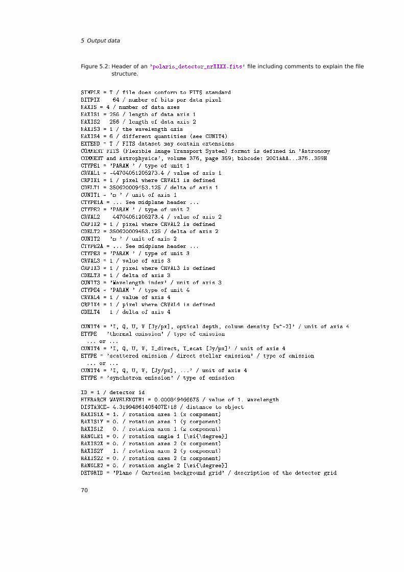
5 Output data
Figure 5.2: Header of an 'polaris_detector_nrXXXX.fits' file including comments to explain the filestructure.
SIMPLE = T / file does conform to FITS standard
BITPIX = -64 / number of bits per data pixel
NAXIS = 4 / number of data axes
NAXIS1 = 256 / length of data axis 1
NAXIS2 = 256 / length of data axis 2
NAXIS3 = 1 / the wavelength axis
NAXIS4 = 6 / different quantities (see CUNIT4)
EXTEND = T / FITS dataset may contain extensions
COMMENT FITS (Flexible Image Transport System) format is defined in 'Astronomy
COMMENT and Astrophysics', volume 376, page 359; bibcode: 2001A&A...376..359H
CTYPE1 = 'PARAM ' / type of unit 1
CRVAL1 = -44704051205273.4 / value of axis 1
CRPIX1 = 1 / pixel where CRVAL1 is defined
CDELT1 = 350620009453.125 / delta of axis 1
CUNIT1 = 'm ' / unit of axis 1
CTYPE1A = ... See midplane header ...
CTYPE2 = 'PARAM ' / type of unit 2
CRVAL2 = -44704051205273.4 / value of axis 2
CRPIX2 = 1 / pixel where CRVAL2 is defined
CDELT2 = 350620009453.125 / delta of axis 2
CUNIT2 = 'm ' / unit of axis 2
CTYPE2A = ... See midplane header ...
CTYPE3 = 'PARAM ' / type of unit 3
CRVAL3 = 1 / value of axis 3
CRPIX3 = 1 / pixel where CRVAL3 is defined
CDELT3 = 1 / delta of axis 3
CUNIT3 = 'Wavelength index' / unit of axis 3
CTYPE4 = 'PARAM ' / type of unit 4
CRVAL4 = 1 / value of axis 4
CRPIX4 = 1 / pixel where CRVAL4 is defined
CDELT4 = 1 / delta of axis 4
CUNIT4 = 'I, Q, U, V [Jy/px], optical depth, column density [m^-2]' / unit of axis 4
ETYPE = 'thermal emission' / type of emission
... or ...
CUNIT4 = 'I, Q, U, V, I_direct, I_scat [Jy/px]' / unit of axis 4
ETYPE = 'scattered emission / direct stellar emission' / type of emission
... or ...
CUNIT4 = 'I, Q, U, V, [Jy/px], ...' / unit of axis 4
ETYPE = 'synchotron emission' / type of emission
ID = 1 / detector id
HIERARCH WAVELENGTH1 = 0.000849466675 / value of 1. wavelength
DISTANCE= 4.31994861405407E+18 / distance to object
RAXIS1X = 1. / rotation axes 1 (x component)
RAXIS1Y = 0. / rotation axes 1 (y component)
RAXIS1Z = 0. / rotation axes 1 (z component)
RANGLE1 = 0. / rotation angle 1 [\si\degree]
RAXIS2X = 0. / rotation axes 2 (x component)
RAXIS2Y = 1. / rotation axes 2 (y component)
RAXIS2Z = 0. / rotation axes 2 (z component)
RANGLE2 = 0. / rotation angle 2 [\si\degree]
DETGRID = 'Plane / Cartesian background grid' / description of the detector grid
70
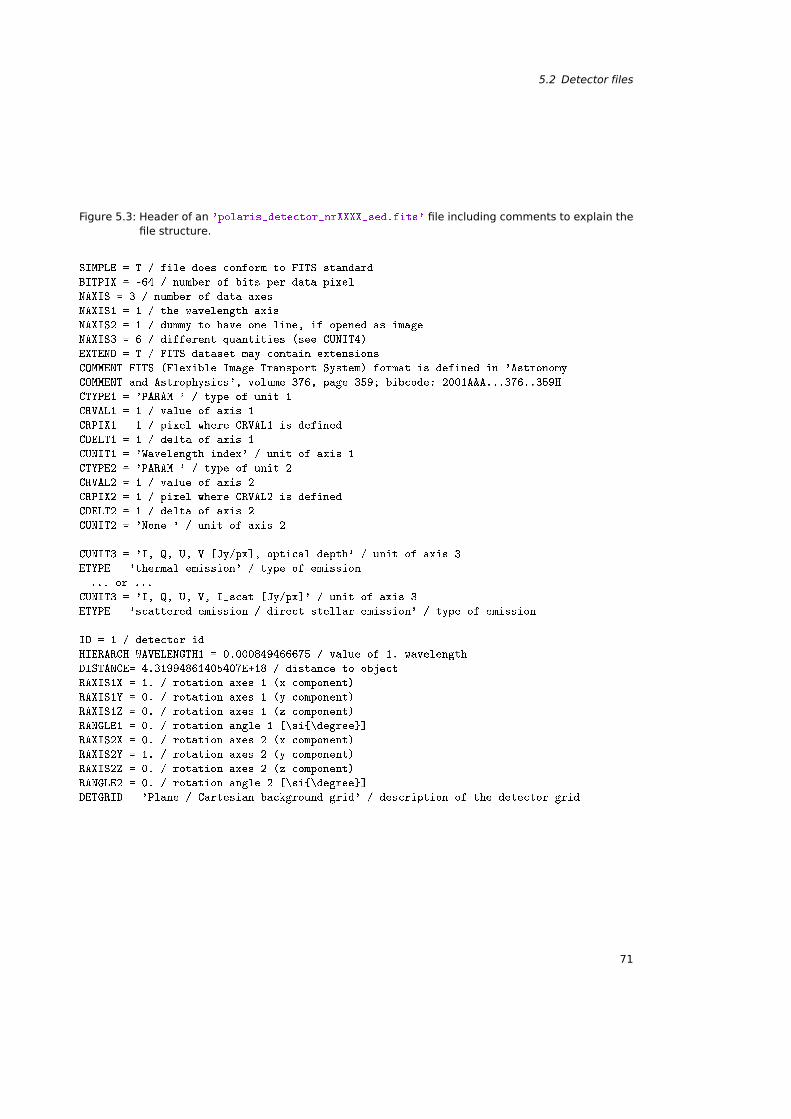
5.2 Detector files
Figure 5.3: Header of an 'polaris_detector_nrXXXX_sed.fits' file including comments to explain thefile structure.
SIMPLE = T / file does conform to FITS standard
BITPIX = -64 / number of bits per data pixel
NAXIS = 3 / number of data axes
NAXIS1 = 1 / the wavelength axis
NAXIS2 = 1 / dummy to have one line, if opened as image
NAXIS3 = 6 / different quantities (see CUNIT4)
EXTEND = T / FITS dataset may contain extensions
COMMENT FITS (Flexible Image Transport System) format is defined in 'Astronomy
COMMENT and Astrophysics', volume 376, page 359; bibcode: 2001A&A...376..359H
CTYPE1 = 'PARAM ' / type of unit 1
CRVAL1 = 1 / value of axis 1
CRPIX1 = 1 / pixel where CRVAL1 is defined
CDELT1 = 1 / delta of axis 1
CUNIT1 = 'Wavelength index' / unit of axis 1
CTYPE2 = 'PARAM ' / type of unit 2
CRVAL2 = 1 / value of axis 2
CRPIX2 = 1 / pixel where CRVAL2 is defined
CDELT2 = 1 / delta of axis 2
CUNIT2 = 'None ' / unit of axis 2
CUNIT3 = 'I, Q, U, V [Jy/px], optical depth' / unit of axis 3
ETYPE = 'thermal emission' / type of emission
... or ...
CUNIT3 = 'I, Q, U, V, I_scat [Jy/px]' / unit of axis 3
ETYPE = 'scattered emission / direct stellar emission' / type of emission
ID = 1 / detector id
HIERARCH WAVELENGTH1 = 0.000849466675 / value of 1. wavelength
DISTANCE= 4.31994861405407E+18 / distance to object
RAXIS1X = 1. / rotation axes 1 (x component)
RAXIS1Y = 0. / rotation axes 1 (y component)
RAXIS1Z = 0. / rotation axes 1 (z component)
RANGLE1 = 0. / rotation angle 1 [\si\degree]
RAXIS2X = 0. / rotation axes 2 (x component)
RAXIS2Y = 1. / rotation axes 2 (y component)
RAXIS2Z = 0. / rotation axes 2 (z component)
RANGLE2 = 0. / rotation angle 2 [\si\degree]
DETGRID = 'Plane / Cartesian background grid' / description of the detector grid
71
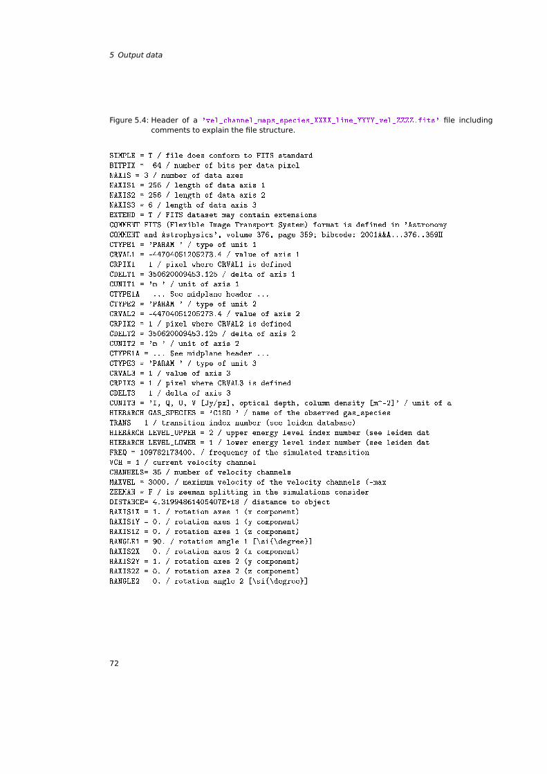
5 Output data
Figure 5.4: Header of a 'vel_channel_maps_species_XXXX_line_YYYY_vel_ZZZZ.fits' file includingcomments to explain the file structure.
SIMPLE = T / file does conform to FITS standard
BITPIX = -64 / number of bits per data pixel
NAXIS = 3 / number of data axes
NAXIS1 = 256 / length of data axis 1
NAXIS2 = 256 / length of data axis 2
NAXIS3 = 6 / length of data axis 3
EXTEND = T / FITS dataset may contain extensions
COMMENT FITS (Flexible Image Transport System) format is defined in 'Astronomy
COMMENT and Astrophysics', volume 376, page 359; bibcode: 2001A&A...376..359H
CTYPE1 = 'PARAM ' / type of unit 1
CRVAL1 = -44704051205273.4 / value of axis 1
CRPIX1 = 1 / pixel where CRVAL1 is defined
CDELT1 = 350620009453.125 / delta of axis 1
CUNIT1 = 'm ' / unit of axis 1
CTYPE1A = ... See midplane header ...
CTYPE2 = 'PARAM ' / type of unit 2
CRVAL2 = -44704051205273.4 / value of axis 2
CRPIX2 = 1 / pixel where CRVAL2 is defined
CDELT2 = 350620009453.125 / delta of axis 2
CUNIT2 = 'm ' / unit of axis 2
CTYPE1A = ... See midplane header ...
CTYPE3 = 'PARAM ' / type of unit 3
CRVAL3 = 1 / value of axis 3
CRPIX3 = 1 / pixel where CRVAL3 is defined
CDELT3 = 1 / delta of axis 3
CUNIT3 = 'I, Q, U, V [Jy/px], optical depth, column density [m^-2]' / unit of a
HIERARCH GAS_SPECIES = 'C18O ' / name of the observed gas_species
TRANS = 1 / transition index number (see leiden database)
HIERARCH LEVEL_UPPER = 2 / upper energy level index number (see leiden dat
HIERARCH LEVEL_LOWER = 1 / lower energy level index number (see leiden dat
FREQ = 109782173400. / frequency of the simulated transition
VCH = 1 / current velocity channel
CHANNELS= 35 / number of velocity channels
MAXVEL = 3000. / maximum velocity of the velocity channels (-max
ZEEMAN = F / is zeeman splitting in the simulations consider
DISTANCE= 4.31994861405407E+18 / distance to object
RAXIS1X = 1. / rotation axes 1 (x component)
RAXIS1Y = 0. / rotation axes 1 (y component)
RAXIS1Z = 0. / rotation axes 1 (z component)
RANGLE1 = 90. / rotation angle 1 [\si\degree]
RAXIS2X = 0. / rotation axes 2 (x component)
RAXIS2Y = 1. / rotation axes 2 (y component)
RAXIS2Z = 0. / rotation axes 2 (z component)
RANGLE2 = 0. / rotation angle 2 [\si\degree]
72
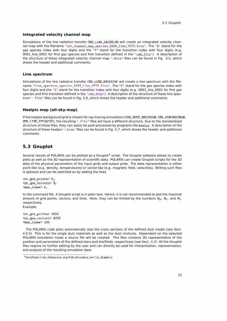
5.3 Gnuplot
Integrated velocity channel map
Simulations of the line radiative transfer CMD_LINE_EMISSION will create an integrated velocity chan-nel map with the filename 'int_channel_map_species_XXXX_line_YYYY.fits'. The 'X' stand for thegas species index with four digits and the 'Y' stand for the transition index with four digits (e.g.0001_line_0001 for first gas species and first transition defined in the 'cmd_file'). A description ofthe structure of these integrated velocity channel map '.fits' files can be found in Fig. 5.5, whichshows the header and additional comments.
Line spectrum
Simulations of the line radiative transfer CMD_LINE_EMISSION will create a line spectrum with the file-name 'line_spectrum_species_XXXX_line_YYYY.fits'. The 'X' stand for the gas species index withfour digits and the 'Y' stand for the transition index with four digits (e.g. 0001_line_0001 for first gasspecies and first transition defined in the 'cmd_file'). A description of the structure of these line spec-trum '.fits' files can be found in Fig. 5.6, which shows the header and additional comments.
Healpix map (all-sky-map)
If the healpix background grid is chosen for ray-tracing simulations (CMD_DUST_EMISSION, CMD_SYNCHROTRON,CMD_LINE_EMISSION), the resulting '.fits' files will have a different structure. Due to the standardizedstructure of these files, they can easily be post-processed by programs like healpy. A description of thestructure of these healpix '.fits' files can be found in Fig. 5.7, which shows the header and additionalcomments.
5.3 Gnuplot
Several results of POLARIS can be plotted as a Gnuplot4 script. The Gnuplot software allows to createplots as well as the 3D representation of scientific data. POLARIS can create Gnuplot scripts for the 3Ddata of the physical parameters of the input grids and output grids. The data representation is eitherpoint-like (e.g. density, temperatures) or vector-like (e.g. magnetic field, velocities). Writing such filesis optional and can be switched on by adding the lines
<nr_gnu_points> Np<nr_gnu_vectors> Nv<max_lines> Nl
to the command file. A Gnuplot script is in plain text. Hence, it is not recommended to plot the maximalamount of grid points, vectors, and lines. Here, they can be limited by the numbers Np , Nv , and N l ,respectively.Example:
<nr_gnu_points> 4000
<nr_gnu_vectors> 4000
<max_lines> 300
The POLARIS code plots automatically also the cross sections of the defined dust model (see Sect.4.6.5). This is for the single dust materials as well as the dust mixtures. Dependent on the selectedPOLARIS simulation mode a source file will be created. This files contains 3D representation of theposition and parameters of the defined stars and starfields, respectively (see Sect. 4.2). All the Gnuplotfiles require no further editing by the user and can directly be used for interpretation, representation,and analysis of the resulting simulation data.
4See https://en.wikipedia.org/wiki/Scalable_Vector_Graphics
73
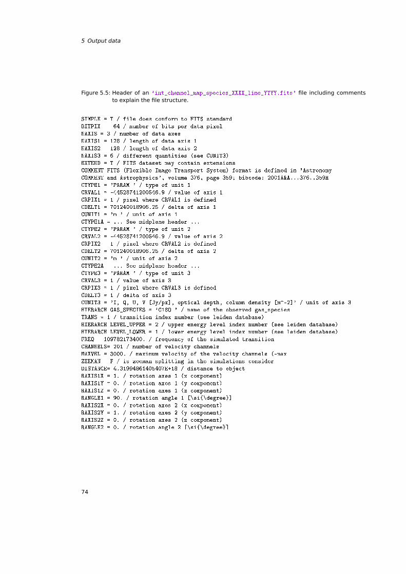
5 Output data
Figure 5.5: Header of an 'int_channel_map_species_XXXX_line_YYYY.fits' file including commentsto explain the file structure.
SIMPLE = T / file does conform to FITS standard
BITPIX = -64 / number of bits per data pixel
NAXIS = 3 / number of data axes
NAXIS1 = 128 / length of data axis 1
NAXIS2 = 128 / length of data axis 2
NAXIS3 = 6 / different quantities (see CUNIT3)
EXTEND = T / FITS dataset may contain extensions
COMMENT FITS (Flexible Image Transport System) format is defined in 'Astronomy
COMMENT and Astrophysics', volume 376, page 359; bibcode: 2001A&A...376..359H
CTYPE1 = 'PARAM ' / type of unit 1
CRVAL1 = -44528741200546.9 / value of axis 1
CRPIX1 = 1 / pixel where CRVAL1 is defined
CDELT1 = 701240018906.25 / delta of axis 1
CUNIT1 = 'm ' / unit of axis 1
CTYPE1A = ... See midplane header ...
CTYPE2 = 'PARAM ' / type of unit 2
CRVAL2 = -44528741200546.9 / value of axis 2
CRPIX2 = 1 / pixel where CRVAL2 is defined
CDELT2 = 701240018906.25 / delta of axis 2
CUNIT2 = 'm ' / unit of axis 2
CTYPE2A = ... See midplane header ...
CTYPE3 = 'PARAM ' / type of unit 3
CRVAL3 = 1 / value of axis 3
CRPIX3 = 1 / pixel where CRVAL3 is defined
CDELT3 = 1 / delta of axis 3
CUNIT3 = 'I, Q, U, V [Jy/px], optical depth, column density [m^-2]' / unit of axis 3
HIERARCH GAS_SPECIES = 'C18O ' / name of the observed gas_species
TRANS = 1 / transition index number (see leiden database)
HIERARCH LEVEL_UPPER = 2 / upper energy level index number (see leiden database)
HIERARCH LEVEL_LOWER = 1 / lower energy level index number (see leiden database)
FREQ = 109782173400. / frequency of the simulated transition
CHANNELS= 201 / number of velocity channels
MAXVEL = 3000. / maximum velocity of the velocity channels (-max
ZEEMAN = F / is zeeman splitting in the simulations consider
DISTANCE= 4.31994861405407E+18 / distance to object
RAXIS1X = 1. / rotation axes 1 (x component)
RAXIS1Y = 0. / rotation axes 1 (y component)
RAXIS1Z = 0. / rotation axes 1 (z component)
RANGLE1 = 90. / rotation angle 1 [\si\degree]
RAXIS2X = 0. / rotation axes 2 (x component)
RAXIS2Y = 1. / rotation axes 2 (y component)
RAXIS2Z = 0. / rotation axes 2 (z component)
RANGLE2 = 0. / rotation angle 2 [\si\degree]
74
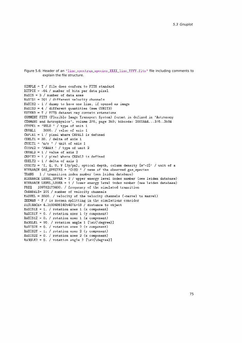
5.3 Gnuplot
Figure 5.6: Header of an 'line_spectrum_species_XXXX_line_YYYY.fits' file including comments toexplain the file structure.
SIMPLE = T / file does conform to FITS standard
BITPIX = -64 / number of bits per data pixel
NAXIS = 3 / number of data axes
NAXIS1 = 201 / different velocity channels
NAXIS2 = 1 / dummy to have one line, if opened as image
NAXIS3 = 4 / different quantities (see CUNIT3)
EXTEND = T / FITS dataset may contain extensions
COMMENT FITS (Flexible Image Transport System) format is defined in 'Astronomy
COMMENT and Astrophysics', volume 376, page 359; bibcode: 2001A&A...376..359H
CTYPE1 = 'VELO ' / type of unit 1
CRVAL1 = -3000. / value of axis 1
CRPIX1 = 1 / pixel where CRVAL1 is defined
CDELT1 = 30. / delta of axis 1
CUNIT1 = 'm/s ' / unit of axis 1
CTYPE2 = 'PARAM ' / type of unit 2
CRVAL2 = 1 / value of axis 2
CRPIX2 = 1 / pixel where CRVAL2 is defined
CDELT2 = 1 / delta of axis 2
CUNIT2 = 'I, Q, U, V [Jy/px], optical depth, column density [m^-2]' / unit of a
HIERARCH GAS_SPECIES = 'C18O ' / name of the observed gas_species
TRANS = 1 / transition index number (see leiden database)
HIERARCH LEVEL_UPPER = 2 / upper energy level index number (see leiden database)
HIERARCH LEVEL_LOWER = 1 / lower energy level index number (see leiden database)
FREQ = 109782173400. / frequency of the simulated transition
CHANNELS= 201 / number of velocity channels
MAXVEL = 3000. / velocity of the velocity channels (-maxvel to maxvel)
ZEEMAN = F / is zeeman splitting in the simulations consider
DISTANCE= 4.31994861405407E+18 / distance to object
RAXIS1X = 1. / rotation axes 1 (x component)
RAXIS1Y = 0. / rotation axes 1 (y component)
RAXIS1Z = 0. / rotation axes 1 (z component)
RANGLE1 = 90. / rotation angle 1 [\si\degree]
RAXIS2X = 0. / rotation axes 2 (x component)
RAXIS2Y = 1. / rotation axes 2 (y component)
RAXIS2Z = 0. / rotation axes 2 (z component)
RANGLE2 = 0. / rotation angle 2 [\si\degree]
75
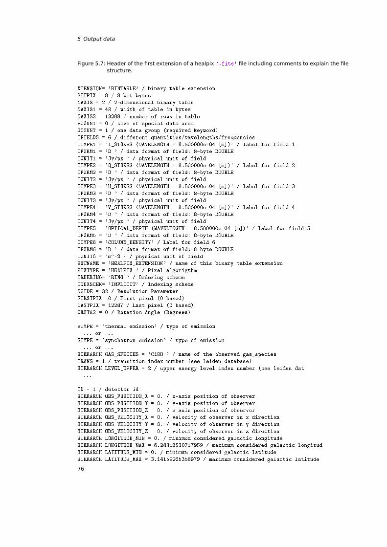
5 Output data
Figure 5.7: Header of the first extension of a healpix '.fits' file including comments to explain the filestructure.
XTENSION= 'BINTABLE' / binary table extension
BITPIX = 8 / 8-bit bytes
NAXIS = 2 / 2-dimensional binary table
NAXIS1 = 48 / width of table in bytes
NAXIS2 = 12288 / number of rows in table
PCOUNT = 0 / size of special data area
GCOUNT = 1 / one data group (required keyword)
TFIELDS = 6 / different quantities/wavelengths/frequencies
TTYPE1 = 'I_STOKES (WAVELENGTH = 8.500000e-04 [m])' / label for field 1
TFORM1 = 'D ' / data format of field: 8-byte DOUBLE
TUNIT1 = 'Jy/px ' / physical unit of field
TTYPE2 = 'Q_STOKES (WAVELENGTH = 8.500000e-04 [m])' / label for field 2
TFORM2 = 'D ' / data format of field: 8-byte DOUBLE
TUNIT2 = 'Jy/px ' / physical unit of field
TTYPE3 = 'U_STOKES (WAVELENGTH = 8.500000e-04 [m])' / label for field 3
TFORM3 = 'D ' / data format of field: 8-byte DOUBLE
TUNIT3 = 'Jy/px ' / physical unit of field
TTYPE4 = 'V_STOKES (WAVELENGTH = 8.500000e-04 [m])' / label for field 4
TFORM4 = 'D ' / data format of field: 8-byte DOUBLE
TUNIT4 = 'Jy/px ' / physical unit of field
TTYPE5 = 'OPTICAL_DEPTH (WAVELENGTH = 8.500000e-04 [m])' / label for field 5
TFORM5 = 'D ' / data format of field: 8-byte DOUBLE
TTYPE6 = 'COLUMN_DENSITY' / label for field 6
TFORM6 = 'D ' / data format of field: 8-byte DOUBLE
TUNIT6 = 'm^-2 ' / physical unit of field
EXTNAME = 'HEALPIX_EXTENSION' / name of this binary table extension
PIXTYPE = 'HEALPIX ' / Pixel algorigthm
ORDERING= 'RING ' / Ordering scheme
INDXSCHM= 'IMPLICIT' / Indexing scheme
NSIDE = 32 / Resolution Parameter
FIRSTPIX= 0 / First pixel (0 based)
LASTPIX = 12287 / Last pixel (0 based)
CROTA2 = 0 / Rotation Angle (Degrees)
ETYPE = 'thermal emission' / type of emission
... or ...
ETYPE = 'synchotron emission' / type of emission
... or ...
HIERARCH GAS_SPECIES = 'C18O ' / name of the observed gas_species
TRANS = 1 / transition index number (see leiden database)
HIERARCH LEVEL_UPPER = 2 / upper energy level index number (see leiden dat
...
ID = 1 / detector id
HIERARCH OBS_POSITION_X = 0. / x-axis position of observer
HIERARCH OBS_POSITION_Y = 0. / y-axis position of observer
HIERARCH OBS_POSITION_Z = 0. / z-axis position of observer
HIERARCH OBS_VELOCITY_X = 0. / velocity of observer in x direction
HIERARCH OBS_VELOCITY_Y = 0. / velocity of observer in y direction
HIERARCH OBS_VELOCITY_Z = 0. / velocity of observer in z direction
HIERARCH LONGITUDE_MIN = 0. / minimum considered galactic longitude
HIERARCH LONGITUDE_MAX = 6.28318530717959 / maximum considered galactic longitud
HIERARCH LATITUDE_MIN = 0. / minimum considered galactic latitude
HIERARCH LATITUDE_MAX = 3.14159265358979 / maximum considered galactic latitude
76
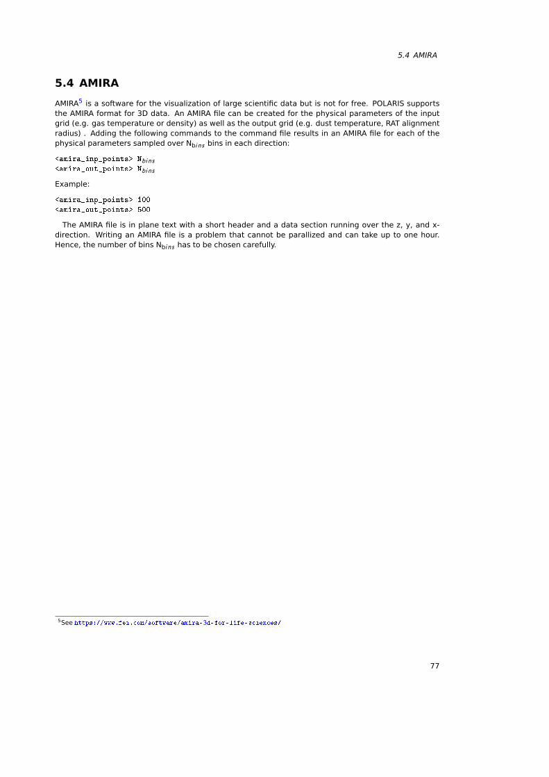
5.4 AMIRA
5.4 AMIRA
AMIRA5 is a software for the visualization of large scientific data but is not for free. POLARIS supportsthe AMIRA format for 3D data. An AMIRA file can be created for the physical parameters of the inputgrid (e.g. gas temperature or density) as well as the output grid (e.g. dust temperature, RAT alignmentradius) . Adding the following commands to the command file results in an AMIRA file for each of thephysical parameters sampled over Nbi ns bins in each direction:
<amira_inp_points> Nbi ns<amira_out_points> Nbi ns
Example:
<amira_inp_points> 100
<amira_out_points> 500
The AMIRA file is in plane text with a short header and a data section running over the z, y, and x-direction. Writing an AMIRA file is a problem that cannot be parallized and can take up to one hour.Hence, the number of bins Nbi ns has to be chosen carefully.
5See https://www.fei.com/software/amira-3d-for-life-sciences/
77

6 Quickstart guide
To try out the main capabilities of POLARIS, use the following step-by-step instruction. The examplesimulations are based on a model of a circumstellar disk with characteristics shown in Table 6.1. Inthis model, we assumes compact, homogeneous, and spherical dust grains with a composition of 62.5%silicate and 37.5% graphite (MRN-dust, Mathis et al. 1977; optical properties from Weingartner & Draine2001).
We consider furthermore a density distribution with a radial decrease based on the work of Hayashi(1981) for the minimum mass solar nebular. Combined with a vertical distribution due to hydrostaticequilibrium similar to the work of Shakura & Sunyaev (1973), we obtain the following equation:
ρdisk = ρ0
(Rref
ω
)aexp
(−12
[z
H (ω)
]2). (6.1)
Here, ω is the radial distance from the central star in the disk midplane, z is the distance from themidplane of the disk, Rref is a reference radius, and H (ω) is the scale height. The density ρ0 is derivedfrom the disk (gas) mass. The scale height is a function of ω as follows:
H (ω) = h0(ω
Rref
)b. (6.2)
The parameters a and b set the radial density profile and the disk flaring, respectively.
6.0.1 Unpack the examples
The first step is to unpack the example package. This package is shipped with POLARIS and includesgrids and command files to perform the following example simulations. To extract the example package,go into your POLARIS directory and enter the following command:
tar -xf examples.tar.xz -C projects/
Now, you have everything you need for the following examples in your projects/disk/ directory. However,to use any of the example command files, the paths to the POLARIS directory has to be adjusted. To dothis, change any occurrence of /YOUR/POLARIS/PATH/ in the command files to your path of the POLARISinstallation.
6.0.2 Dust temperature distribution
The dust temperature distribution can be simulated by assuming that the dust grains are in equilibriumwith the radiation field. To do this, enter the following command (t ∼ 3min):
polaris /YOUR/POLARIS/PATH/projects/disk/example/temp/POLARIS.cmd
The temperature distribution can be visualized with the '.fits' file viewer ds9. You find the '.fits'
files in the projects/disk/example/temp/data/ directory. The temperature distributions should look likethose in Fig. 7.1. The creation of proper plots can be realized by e.g. Python scripts using matplotlib
and astropy. However, especially if you do not have similar scripts, we suggest to use our toolkitPolarisTools for visualization (see 7).
79
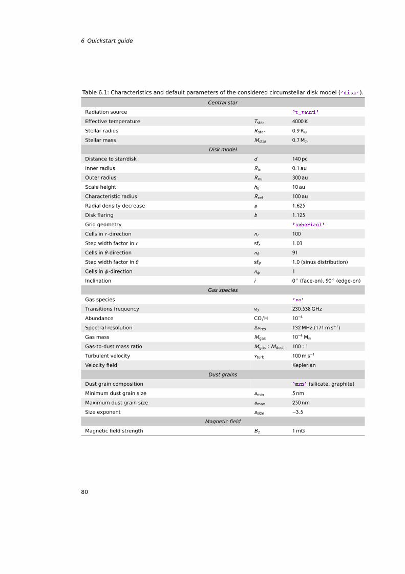
6 Quickstart guide
Table 6.1: Characteristics and default parameters of the considered circumstellar disk model ('disk').
Central star
Radiation source 't_tauri'
Effective temperature Tstar 4000K
Stellar radius Rstar 0.9R
Stellar mass Mstar 0.7M
Disk model
Distance to star/disk d 140pc
Inner radius R in 0.1 au
Outer radius Rou 300 au
Scale height h0 10 au
Characteristic radius Rref 100 au
Radial density decrease a 1.625
Disk flaring b 1.125
Grid geometry 'spherical'
Cells in r -direction nr 100
Step width factor in r sfr 1.03
Cells in θ-direction nθ 91
Step width factor in θ sfθ 1.0 (sinus distribution)
Cells in φ-direction nφ 1
Inclination i 0 (face-on), 90 (edge-on)
Gas species
Gas species 'co'
Transitions frequency ν0 230.538GHz
Abundance CO/H 10−4
Spectral resolution ∆νres 132MHz (171m s−1)Gas mass Mgas 10−4 M
Gas-to-dust mass ratio Mgas : Mdust 100 : 1
Turbulent velocity vturb 100m s−1
Velocity field Keplerian
Dust grains
Dust grain composition 'mrn' (silicate, graphite)
Minimum dust grain size amin 5nm
Maximum dust grain size amax 250nm
Size exponent asize −3.5Magnetic field
Magnetic field strength Bz 1mG
80
6.0.3 Dust thermal emission
Based on the dust temperature distribution, the thermal emission of the dust grains at λ ∼ 850µm canbe simulated. To do this, enter the following command (t ∼ 30 s):
polaris /YOUR/POLARIS/PATH/projects/disk/example/dust/POLARIS.cmd
You find the '.fits' files in the projects/disk/example/dust/data/ directory. The intensity map shouldlook like Fig. 7.2 (left).
6.0.4 Dust thermal emission (with grain alignment)
Based on the dust temperature distribution, the thermal emission of aligned non-spherical dust grainsat λ ∼ 850µm can be simulated. To do this, enter the following command (t ∼ 30 s):
polaris /YOUR/POLARIS/PATH/projects/disk/example/dust_pa/POLARIS.cmd
In this simulation, the disk is observed edge-on and the spherical dust grains will be replaced byoblate dust grains which are perfectly perpendicular aligned with their longest axis to the magneticfield. Since this guide only shows the capabilities of POLARIS, it is sufficient to use the dust tem-perature distribution which was simulated with spherical dust grains. Otherwise, the temperaturedistribution needs to be calculated again with oblate dust grains. You find the '.fits' files in theprojects/disk/example/dust_pa/data/ directory. The intensity map should look like Fig. 7.3 (left).
6.0.5 Scattered stellar emission
Based on the dust density distribution, the stellar radiation at λ = 1µm scattered at the spherical dustgrains can be simulated. To do this, enter the following command (t ∼ 5min):
polaris /YOUR/POLARIS/PATH/projects/disk/example/dust_mc/POLARIS.cmd
The disk is inclined by 60 to achieve a better visual impression of the scattered light. You find the'.fits' files in the projects/disk/example/dust_mc/data/ directory. Polarization maps can be calculatedfrom these '.fits' files that should look like Fig. 7.4 (top).
6.0.6 Thermal emission and scattered stellar emission
The stellar emission scattered at spherical dust grains can also be included in the thermal emissioncalculation. To do this, the temperature calculation needs to be repeated with the <radiation_field> 1
option by entering the following command (t ∼ 2min):
polaris /YOUR/POLARIS/PATH/projects/disk/example2/temp/POLARIS.cmd
Then, the thermal emission and scattered stellar emission of the dust grains at λ = 1µm can be simu-lated. To do this, enter the following command (t ∼ 5min):
polaris /YOUR/POLARIS/PATH/projects/disk/example2/dust/POLARIS.cmd
The disk is inclined by 60 to achieve a better visual impression of the scattered light. You find the'.fits' files in the projects/disk/example2/dust/data/ directory. Polarization maps can be calculatedfrom these '.fits' files that should look like Fig. 7.4 (bottom).
6.0.7 Spectral line emission
Based on the gas temperature distribution, the spectral line emission of the C18O J = 1 → 0 transition(ν ∼ 109GHz) can be simulated. To do this, enter the following command (t ∼ 5min):
polaris /YOUR/POLARIS/PATH/projects/disk/example/line/POLARIS.cmd
81
6 Quickstart guide
In this simulation, the disk is observed edge-on and the Keplerian rotation around the central star is con-sidered for the velocity field. You find the '.fits' files in the projects/disk/example/line/data/ directory.The velocity channel map, integrated velocity channel map and spectrum should look like Fig. 7.5 (top,middle).
6.0.8 Spectral line emission (with Zeeman splitting)
Based on the gas temperature distribution, the Zeeman split spectral line emission of the OH transitionat ν ∼ 1665MHz can be simulated (see Brauer et al. 2017a). To do this, enter the following command(t ∼ 60min):
polaris /YOUR/POLARIS/PATH/projects/disk/example/zeeman/POLARIS.cmd
In this simulation, the disk is observed face-on and, therefore, the Keplerian rotation is not required.You find the '.fits' files in the projects/disk/example/zeeman/data/ directory. The circular polarizationspectrum should look like Fig. 7.5 (bottom right). Magnetic field maps calculated via the Zeemananalysis can be obtained with PolarisTools (see 7).
82
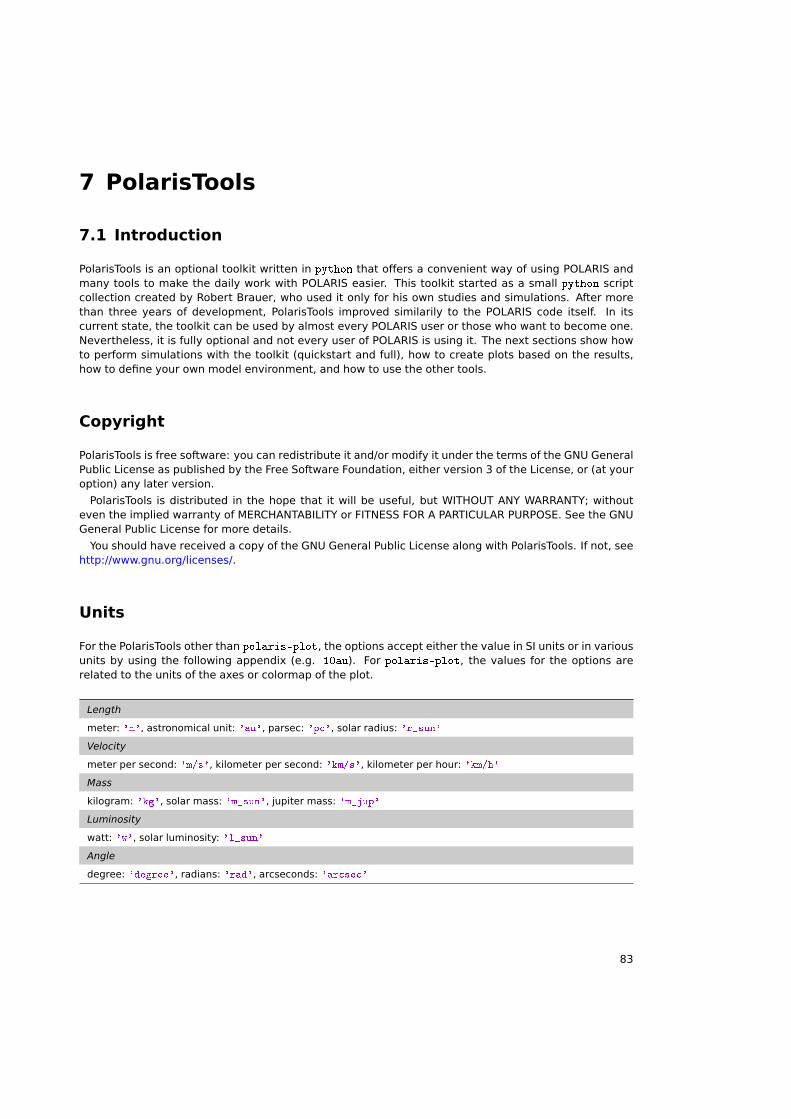
7 PolarisTools
7.1 Introduction
PolarisTools is an optional toolkit written in python that offers a convenient way of using POLARIS andmany tools to make the daily work with POLARIS easier. This toolkit started as a small python scriptcollection created by Robert Brauer, who used it only for his own studies and simulations. After morethan three years of development, PolarisTools improved similarily to the POLARIS code itself. In itscurrent state, the toolkit can be used by almost every POLARIS user or those who want to become one.Nevertheless, it is fully optional and not every user of POLARIS is using it. The next sections show howto perform simulations with the toolkit (quickstart and full), how to create plots based on the results,how to define your own model environment, and how to use the other tools.
Copyright
PolarisTools is free software: you can redistribute it and/or modify it under the terms of the GNU GeneralPublic License as published by the Free Software Foundation, either version 3 of the License, or (at youroption) any later version.
PolarisTools is distributed in the hope that it will be useful, but WITHOUT ANY WARRANTY; withouteven the implied warranty of MERCHANTABILITY or FITNESS FOR A PARTICULAR PURPOSE. See the GNUGeneral Public License for more details.
You should have received a copy of the GNU General Public License along with PolarisTools. If not, seehttp://www.gnu.org/licenses/.
Units
For the PolarisTools other than polaris-plot, the options accept either the value in SI units or in variousunits by using the following appendix (e.g. 10au). For polaris-plot, the values for the options arerelated to the units of the axes or colormap of the plot.
Length
meter: 'm', astronomical unit: 'au', parsec: 'pc', solar radius: 'r_sun'
Velocity
meter per second: 'm/s', kilometer per second: 'km/s', kilometer per hour: 'km/h'
Mass
kilogram: 'kg', solar mass: 'm_sun', jupiter mass: 'm_jup'
Luminosity
watt: 'w', solar luminosity: 'l_sun'
Angle
degree: 'degree', radians: 'rad', arcseconds: 'arcsec'
83
7 PolarisTools
7.2 The command polaris-gen
This tool can be used to create a grid based on a given model (model_name). To create a grid, enter thefollowing command:
polaris-gen model_name grid_name.dat
See Sect. 7.7 for available model names.
Available options
The Tables 7.1 and 7.2 show an overview of the available options to modify the creation of a grid withpolaris-gen.
7.3 The command polaris-run
This tool can be used to perform a simulation with POLARIS based on a given model (see Sect. 7.7for available model names). By defining a name of the simulation (simulation_name), the results ofdifferent simulations will be saved in:
• projects/model_name/simulation_name/simulation_type/
Simulation types
The following commands give an overview of all available simulations that can be performed with PO-LARIS.
Dust temperature distribution
To calculate the dust temperature distribution based on the radiation field, enter the following command:
polaris-run model_name simulation_name temp
Use --adj_tgas 1 to apply the dust temperature distribution also for the gas phase.
Radiative torque calculation
To calculate the necessary information to consider Radiative torque alignment, enter the following com-mand:
polaris-run model_name simulation_name rat
The grid will be taken from a previous temperature calculation with the same simulation name.
Temperature and RAT calculation
The calculations of the dust temperature and radiative torque can be performed together by enteringthe following command:
polaris-run model_name simulation_name temp_rat
This simulation type behaves in terms of options the same as the temperature calculation.
84
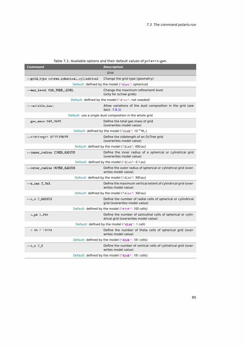
7.3 The command polaris-run
Table 7.1: Available options and their default values of polaris-gen.
Command Description
Grid
--grid_type octree,spherical,cylindrical Change the grid type (geometry)
Default: defined by the model ('disk': spherical)
--max_level MAX_TREE_LEVEL Change the maximum refinement level(only for octree grids)
Default: defined by the model ('disk': not needed)
--variable_dust Allow variations of the dust composition in the grid (seeSect. 7.8.1)
Default: use a single dust composition in the whole grid
--gas_mass GAS_MASS Define the total gas mass of grid(overwrites model value)
Default: defined by the model ('disk': 10−4 M)
--sidelength SIDELENGTH Define the sidelength of an OcTree grid(overwrites model value)
Default: defined by the model ('disk': 600 au)
--inner_radius INNER_RADIUS Define the inner radius of a spherical or cylindrical grid(overwrites model value)
Default: defined by the model ('disk': 0.1 au)
--outer_radius OUTER_RADIUS Define the outer radius of spherical or cylindrical grid (over-writes model value)
Default: defined by the model ('disk': 300 au)
--z_max Z_MAX Define the maximum vertical extent of cylindrical grid (over-writes model value)
Default: defined by the model ('disk': 300 au)
--n_r N_RADIUS Define the number of radial cells of spherical or cylindricalgrid (overwrites model value)
Default: defined by the model ('disk': 100 cells)
--n_ph N_PHI Define the number of azimuthal cells of spherical or cylin-drical grid (overwrites model value)
Default: defined by the model ('disk': 1 cell)
--n_th N_THETA Define the number of theta cells of spherical grid (over-writes model value)
Default: defined by the model ('disk': 181 cells)
--n_z N_Z Define the number of vertical cells of cylindrical grid (over-writes model value)
Default: defined by the model ('disk': 181 cells)
85
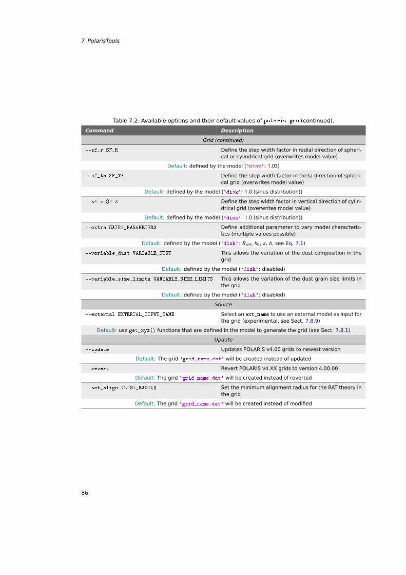
7 PolarisTools
Table 7.2: Available options and their default values of polaris-gen (continued).
Command Description
Grid (continued)
--sf_r SF_R Define the step width factor in radial direction of spheri-cal or cylindrical grid (overwrites model value)
Default: defined by the model ('disk': 1.03)
--sf_th SF_TH Define the step width factor in theta direction of spheri-cal grid (overwrites model value)
Default: defined by the model ('disk': 1.0 (sinus distribution))
--sf_z SF_Z Define the step width factor in vertical direction of cylin-drical grid (overwrites model value)
Default: defined by the model ('disk': 1.0 (sinus distribution))
--extra EXTRA_PARAMETERS Define additional parameter to vary model characteris-tics (multiple values possible)
Default: defined by the model ('disk': Rref, h0, a, b, see Eq. 7.1)
--variable_dust VARIABLE_DUST This allows the variation of the dust composition in thegrid
Default: defined by the model ('disk': disabled)
--variable_size_limits VARIABLE_SIZE_LIMITS This allows the variation of the dust grain size limits inthe grid
Default: defined by the model ('disk': disabled)
Source
--external EXTERNAL_INPUT_NAME Select an ext_name to use an external model as input forthe grid (experimental, see Sect. 7.8.9)
Default: use get_xyz() functions that are defined in the model to generate the grid (see Sect. 7.8.1)
Update
--update Updates POLARIS v4.00 grids to newest version
Default: The grid 'grid_name.dat' will be created instead of updated
--revert Revert POLARIS v4.XX grids to version 4.00.00
Default: The grid 'grid_name.dat' will be created instead of reverted
--set_align ALIGN_RADIUS Set the minimum alignment radius for the RAT theory inthe grid
Default: The grid 'grid_name.dat' will be created instead of modified
86
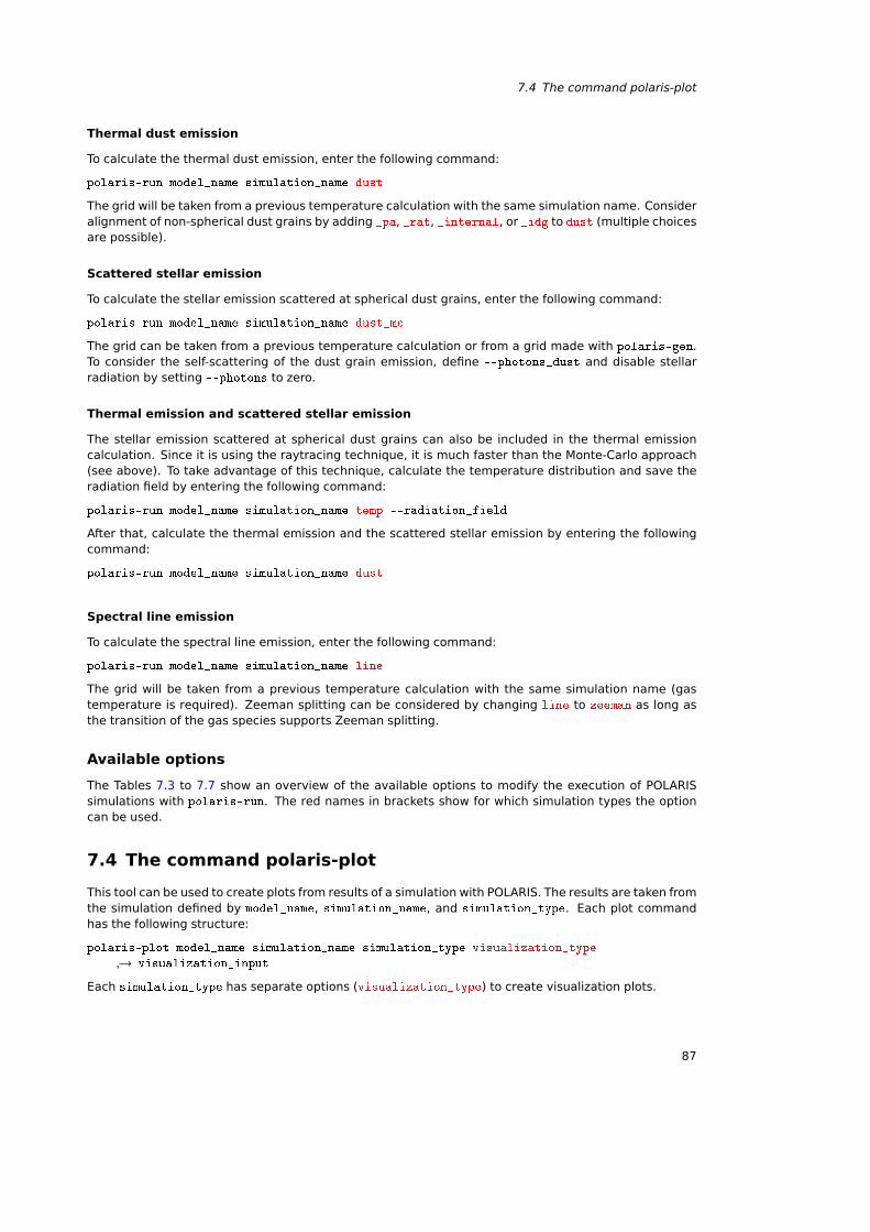
7.4 The command polaris-plot
Thermal dust emission
To calculate the thermal dust emission, enter the following command:
polaris-run model_name simulation_name dust
The grid will be taken from a previous temperature calculation with the same simulation name. Consideralignment of non-spherical dust grains by adding _pa, _rat, _internal, or _idg to dust (multiple choicesare possible).
Scattered stellar emission
To calculate the stellar emission scattered at spherical dust grains, enter the following command:
polaris-run model_name simulation_name dust_mc
The grid can be taken from a previous temperature calculation or from a grid made with polaris-gen.To consider the self-scattering of the dust grain emission, define --photons_dust and disable stellarradiation by setting --photons to zero.
Thermal emission and scattered stellar emission
The stellar emission scattered at spherical dust grains can also be included in the thermal emissioncalculation. Since it is using the raytracing technique, it is much faster than the Monte-Carlo approach(see above). To take advantage of this technique, calculate the temperature distribution and save theradiation field by entering the following command:
polaris-run model_name simulation_name temp --radiation_field
After that, calculate the thermal emission and the scattered stellar emission by entering the followingcommand:
polaris-run model_name simulation_name dust
Spectral line emission
To calculate the spectral line emission, enter the following command:
polaris-run model_name simulation_name line
The grid will be taken from a previous temperature calculation with the same simulation name (gastemperature is required). Zeeman splitting can be considered by changing line to zeeman as long asthe transition of the gas species supports Zeeman splitting.
Available options
The Tables 7.3 to 7.7 show an overview of the available options to modify the execution of POLARISsimulations with polaris-run. The red names in brackets show for which simulation types the optioncan be used.
7.4 The command polaris-plot
This tool can be used to create plots from results of a simulation with POLARIS. The results are taken fromthe simulation defined by model_name, simulation_name, and simulation_type. Each plot commandhas the following structure:
polaris-plot model_name simulation_name simulation_type visualization_type
→ visualization_input
Each simulation_type has separate options (visualization_type) to create visualization plots.
87
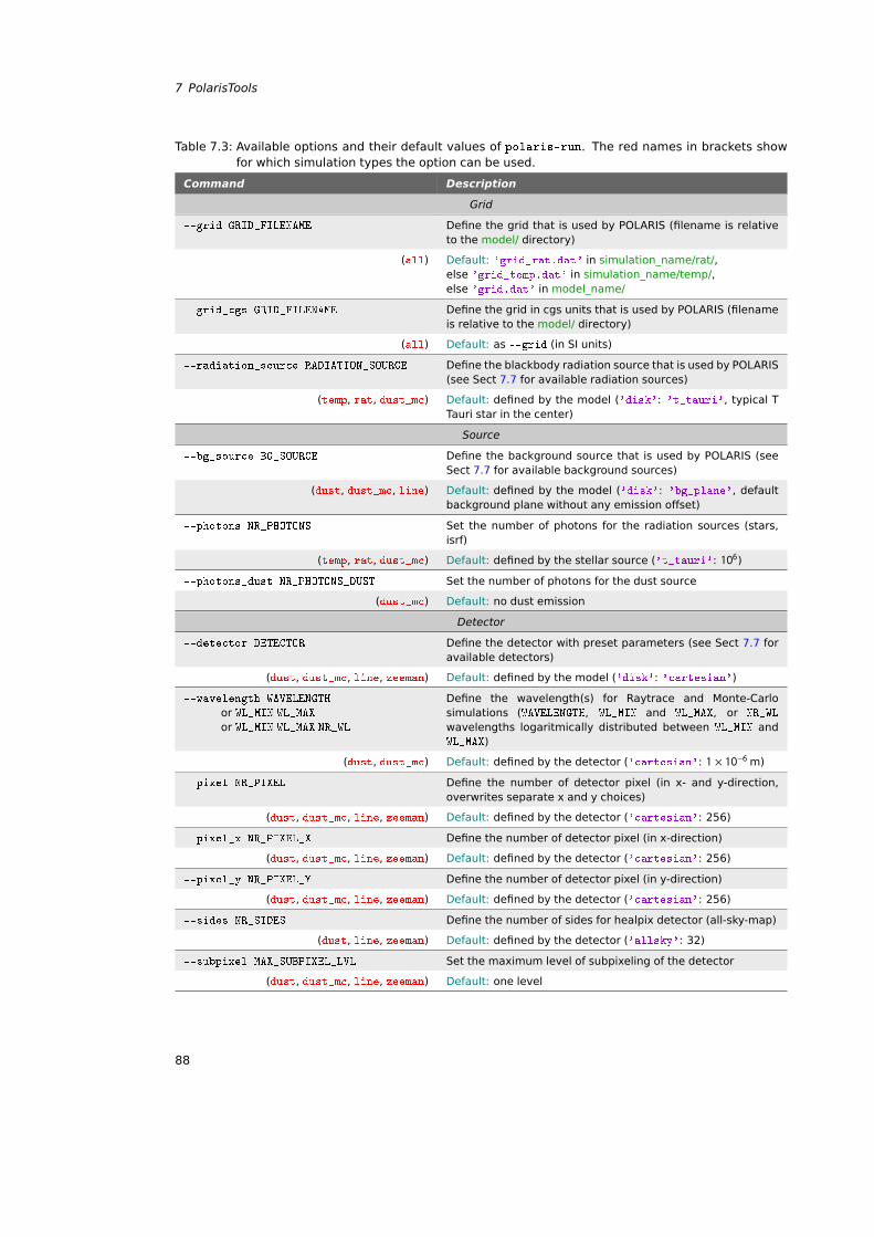
7 PolarisTools
Table 7.3: Available options and their default values of polaris-run. The red names in brackets showfor which simulation types the option can be used.
Command Description
Grid
--grid GRID_FILENAME Define the grid that is used by POLARIS (filename is relativeto the model/ directory)
(all) Default: 'grid_rat.dat' in simulation_name/rat/,else 'grid_temp.dat' in simulation_name/temp/,else 'grid.dat' in model_name/
--grid_cgs GRID_FILENAME Define the grid in cgs units that is used by POLARIS (filenameis relative to the model/ directory)
(all) Default: as --grid (in SI units)
--radiation_source RADIATION_SOURCE Define the blackbody radiation source that is used by POLARIS(see Sect 7.7 for available radiation sources)
(temp, rat, dust_mc) Default: defined by the model ('disk': 't_tauri', typical TTauri star in the center)
Source
--bg_source BG_SOURCE Define the background source that is used by POLARIS (seeSect 7.7 for available background sources)
(dust, dust_mc, line) Default: defined by the model ('disk': 'bg_plane', defaultbackground plane without any emission offset)
--photons NR_PHOTONS Set the number of photons for the radiation sources (stars,isrf)
(temp, rat, dust_mc) Default: defined by the stellar source ('t_tauri': 106)
--photons_dust NR_PHOTONS_DUST Set the number of photons for the dust source
(dust_mc) Default: no dust emission
Detector
--detector DETECTOR Define the detector with preset parameters (see Sect 7.7 foravailable detectors)
(dust, dust_mc, line, zeeman) Default: defined by the model ('disk': 'cartesian')
--wavelength WAVELENGTH
or WL_MIN WL_MAX
or WL_MIN WL_MAX NR_WL
Define the wavelength(s) for Raytrace and Monte-Carlosimulations (WAVELENGTH, WL_MIN and WL_MAX, or NR_WL
wavelengths logaritmically distributed between WL_MIN andWL_MAX)
(dust, dust_mc) Default: defined by the detector ('cartesian': 1 × 10⁻⁶ m)
--pixel NR_PIXEL Define the number of detector pixel (in x- and y-direction,overwrites separate x and y choices)
(dust, dust_mc, line, zeeman) Default: defined by the detector ('cartesian': 256)
--pixel_x NR_PIXEL_X Define the number of detector pixel (in x-direction)
(dust, dust_mc, line, zeeman) Default: defined by the detector ('cartesian': 256)
--pixel_y NR_PIXEL_Y Define the number of detector pixel (in y-direction)
(dust, dust_mc, line, zeeman) Default: defined by the detector ('cartesian': 256)
--sides NR_SIDES Define the number of sides for healpix detector (all-sky-map)
(dust, line, zeeman) Default: defined by the detector ('allsky': 32)
--subpixel MAX_SUBPIXEL_LVL Set the maximum level of subpixeling of the detector
(dust, dust_mc, line, zeeman) Default: one level
88
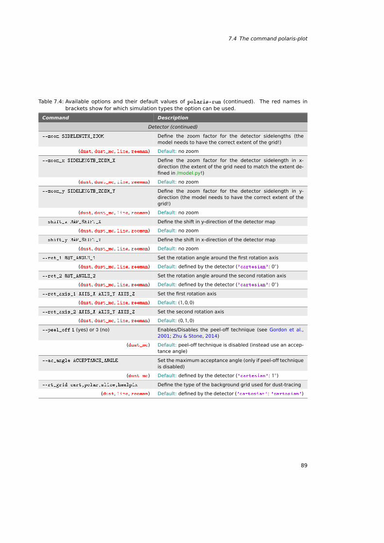
7.4 The command polaris-plot
Table 7.4: Available options and their default values of polaris-run (continued). The red names inbrackets show for which simulation types the option can be used.
Command Description
Detector (continued)
--zoom SIDELENGTH_ZOOM Define the zoom factor for the detector sidelengths (themodel needs to have the correct extent of the grid!)
(dust, dust_mc, line, zeeman) Default: no zoom
--zoom_x SIDELENGTH_ZOOM_X Define the zoom factor for the detector sidelength in x-direction (the extent of the grid need to match the extent de-fined in /model.py!)
(dust, dust_mc, line, zeeman) Default: no zoom
--zoom_y SIDELENGTH_ZOOM_Y Define the zoom factor for the detector sidelength in y-direction (the model needs to have the correct extent of thegrid!)
(dust, dust_mc, line, zeeman) Default: no zoom
--shift_x MAP_SHIFT_X Define the shift in y-direction of the detector map
(dust, dust_mc, line, zeeman) Default: no zoom
--shift_y MAP_SHIFT_Y Define the shift in x-direction of the detector map
(dust, dust_mc, line, zeeman) Default: no zoom
--rot_1 ROT_ANGLE_1 Set the rotation angle around the first rotation axis
(dust, dust_mc, line, zeeman) Default: defined by the detector ('cartesian': 0)
--rot_2 ROT_ANGLE_2 Set the rotation angle around the second rotation axis
(dust, dust_mc, line, zeeman) Default: defined by the detector ('cartesian': 0)
--rot_axis_1 AXIS_X AXIS_Y AXIS_Z Set the first rotation axis
(dust, dust_mc, line, zeeman) Default: (1, 0, 0)--rot_axis_2 AXIS_X AXIS_Y AXIS_Z Set the second rotation axis
(dust, dust_mc, line, zeeman) Default: (0, 1, 0)--peel_off 1 (yes) or 0 (no) Enables/Disables the peel-off technique (see Gordon et al.,
2001; Zhu & Stone, 2014)
(dust_mc) Default: peel-off technique is disabled (instead use an accep-tance angle)
--ac_angle ACCEPTANCE_ANGLE Set the maximum acceptance angle (only if peel-off techniqueis disabled)
(dust_mc) Default: defined by the detector ('cartesian': 1)
--rt_grid cart,polar,slice,healpix Define the type of the background grid used for dust-tracing
(dust, line, zeeman) Default: defined by the detector ('cartesian': 'cartesian')
89
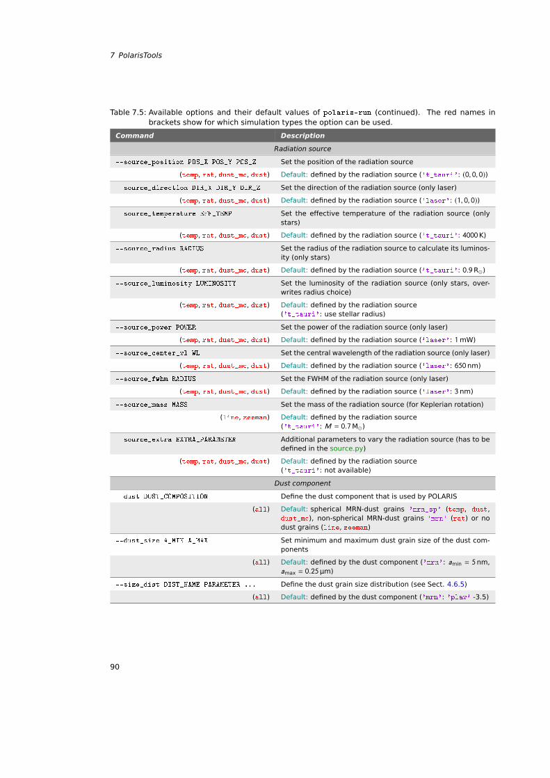
7 PolarisTools
Table 7.5: Available options and their default values of polaris-run (continued). The red names inbrackets show for which simulation types the option can be used.
Command Description
Radiation source
--source_position POS_X POS_Y POS_Z Set the position of the radiation source
(temp, rat, dust_mc, dust) Default: defined by the radiation source ('t_tauri': (0, 0, 0))--source_direction DIR_X DIR_Y DIR_Z Set the direction of the radiation source (only laser)
(temp, rat, dust_mc, dust) Default: defined by the radiation source ('laser': (1, 0, 0))--source_temperature EFF_TEMP Set the effective temperature of the radiation source (only
stars)
(temp, rat, dust_mc, dust) Default: defined by the radiation source ('t_tauri': 4000K)
--source_radius RADIUS Set the radius of the radiation source to calculate its luminos-ity (only stars)
(temp, rat, dust_mc, dust) Default: defined by the radiation source ('t_tauri': 0.9R)
--source_luminosity LUMINOSITY Set the luminosity of the radiation source (only stars, over-writes radius choice)
(temp, rat, dust_mc, dust) Default: defined by the radiation source('t_tauri': use stellar radius)
--source_power POWER Set the power of the radiation source (only laser)
(temp, rat, dust_mc, dust) Default: defined by the radiation source ('laser': 1mW)
--source_center_wl WL Set the central wavelength of the radiation source (only laser)
(temp, rat, dust_mc, dust) Default: defined by the radiation source ('laser': 650nm)
--source_fwhm RADIUS Set the FWHM of the radiation source (only laser)
(temp, rat, dust_mc, dust) Default: defined by the radiation source ('laser': 3nm)
--source_mass MASS Set the mass of the radiation source (for Keplerian rotation)
(line, zeeman) Default: defined by the radiation source('t_tauri': M = 0.7M)
--source_extra EXTRA_PARAMETER Additional parameters to vary the radiation source (has to bedefined in the source.py)
(temp, rat, dust_mc, dust) Default: defined by the radiation source('t_tauri': not available)
Dust component
--dust DUST_COMPOSITION Define the dust component that is used by POLARIS
(all) Default: spherical MRN-dust grains 'mrn_sp' (temp, dust,dust_mc), non-spherical MRN-dust grains 'mrn' (rat) or nodust grains (line, zeeman)
--dust_size A_MIN A_MAX Set minimum and maximum dust grain size of the dust com-ponents
(all) Default: defined by the dust component ('mrn': amin = 5nm,amax = 0.25µm)
--size_dist DIST_NAME PARAMETER ... Define the dust grain size distribution (see Sect. 4.6.5)
(all) Default: defined by the dust component ('mrn': 'plaw' -3.5)
90
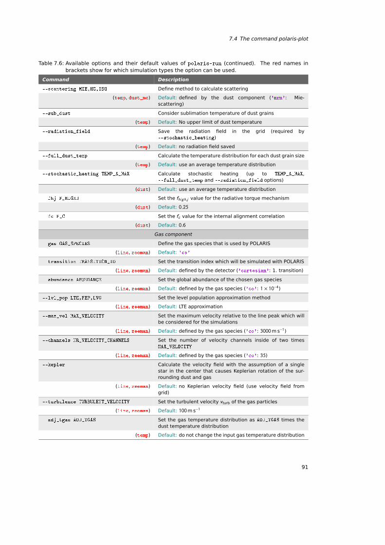
7.4 The command polaris-plot
Table 7.6: Available options and their default values of polaris-run (continued). The red names inbrackets show for which simulation types the option can be used.
Command Description
--scattering MIE,HG,ISO Define method to calculate scattering
(temp, dust_mc) Default: defined by the dust component ('mrn': Mie-scattering)
--sub_dust Consider sublimation temperature of dust grains
(temp) Default: No upper limit of dust temperature
--radiation_field Save the radiation field in the grid (required by--stochastic_heating)
(temp) Default: no radiation field saved
--full_dust_temp Calculate the temperature distribution for each dust grain size
(temp) Default: use an average temperature distribution
--stochastic_heating TEMP_A_MAX Calculate stochastic heating (up to TEMP_A_MAX,--full_dust_temp and --radiation_field options)
(dust) Default: use an average temperature distribution
--fhj F_HIGHJ Set the fhi gh,j value for the radiative torque mechanism
(dust) Default: 0.25
--fc F_C Set the fc value for the internal alignment correlation
(dust) Default: 0.6
Gas component
--gas GAS_SPECIES Define the gas species that is used by POLARIS
(line, zeeman) Default: 'co'
--transition TRANSITION_ID Set the transition index which will be simulated with POLARIS
(line, zeeman) Default: defined by the detector ('cartesian': 1. transition)
--abundance ABUNDANCE Set the global abundance of the chosen gas species
(line, zeeman) Default: defined by the gas species ('co': 1 × 10⁻⁴)--lvl_pop LTE,FEP,LVG Set the level population approximation method
(line, zeeman) Default: LTE approximation
--max_vel MAX_VELOCITY Set the maximum velocity relative to the line peak which willbe considered for the simulations
(line, zeeman) Default: defined by the gas species ('co': 3000m s−1)
--channels NR_VELOCITY_CHANNELS Set the number of velocity channels inside of two timesMAX_VELOCITY
(line, zeeman) Default: defined by the gas species ('co': 35)
--kepler Calculate the velocity field with the assumption of a singlestar in the center that causes Keplerian rotation of the sur-rounding dust and gas
(line, zeeman) Default: no Keplerian velocity field (use velocity field fromgrid)
--turbulence TURBULENT_VELOCITY Set the turbulent velocity vturb of the gas particles
(line, zeeman) Default: 100m s−1
--adj_tgas ADJ_TGAS Set the gas temperature distribution as ADJ_TGAS times thedust temperature distribution
(temp) Default: do not change the input gas temperature distribution
91
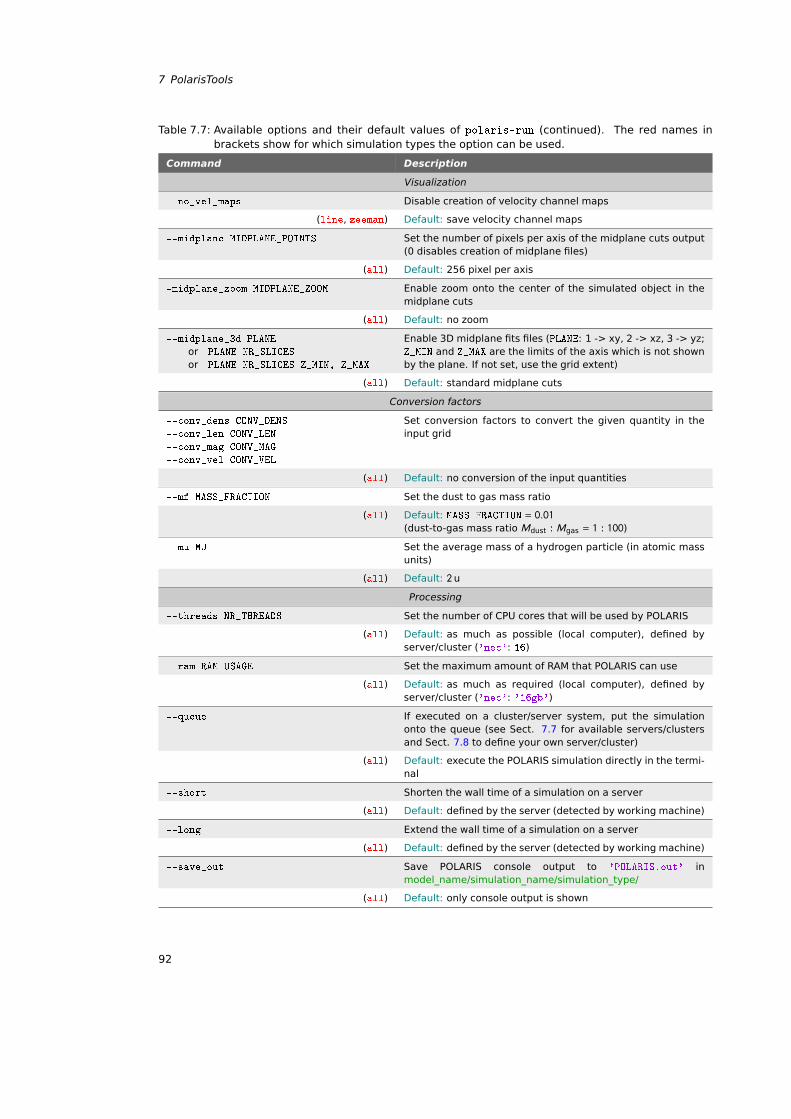
7 PolarisTools
Table 7.7: Available options and their default values of polaris-run (continued). The red names inbrackets show for which simulation types the option can be used.
Command Description
Visualization
--no_vel_maps Disable creation of velocity channel maps
(line, zeeman) Default: save velocity channel maps
--midplane MIDPLANE_POINTS Set the number of pixels per axis of the midplane cuts output(0 disables creation of midplane files)
(all) Default: 256 pixel per axis
-midplane_zoom MIDPLANE_ZOOM Enable zoom onto the center of the simulated object in themidplane cuts
(all) Default: no zoom
--midplane_3d PLANE
or PLANE NR_SLICES
or PLANE NR_SLICES Z_MIN, Z_MAX
Enable 3D midplane fits files (PLANE: 1 -> xy, 2 -> xz, 3 -> yz;Z_MIN and Z_MAX are the limits of the axis which is not shownby the plane. If not set, use the grid extent)
(all) Default: standard midplane cuts
Conversion factors
--conv_dens CONV_DENS
--conv_len CONV_LEN
--conv_mag CONV_MAG
--conv_vel CONV_VEL
Set conversion factors to convert the given quantity in theinput grid
(all) Default: no conversion of the input quantities
--mf MASS_FRACTION Set the dust to gas mass ratio
(all) Default: MASS_FRACTION = 0.01(dust-to-gas mass ratio Mdust : Mgas = 1 : 100)
--mu MU Set the average mass of a hydrogen particle (in atomic massunits)
(all) Default: 2u
Processing
--threads NR_THREADS Set the number of CPU cores that will be used by POLARIS
(all) Default: as much as possible (local computer), defined byserver/cluster ('nec': 16)
--ram RAM_USAGE Set the maximum amount of RAM that POLARIS can use
(all) Default: as much as required (local computer), defined byserver/cluster ('nec': '16gb')
--queue If executed on a cluster/server system, put the simulationonto the queue (see Sect. 7.7 for available servers/clustersand Sect. 7.8 to define your own server/cluster)
(all) Default: execute the POLARIS simulation directly in the termi-nal
--short Shorten the wall time of a simulation on a server
(all) Default: defined by the server (detected by working machine)
--long Extend the wall time of a simulation on a server
(all) Default: defined by the server (detected by working machine)
--save_out Save POLARIS console output to 'POLARIS.out' inmodel_name/simulation_name/simulation_type/
(all) Default: only console output is shown
92
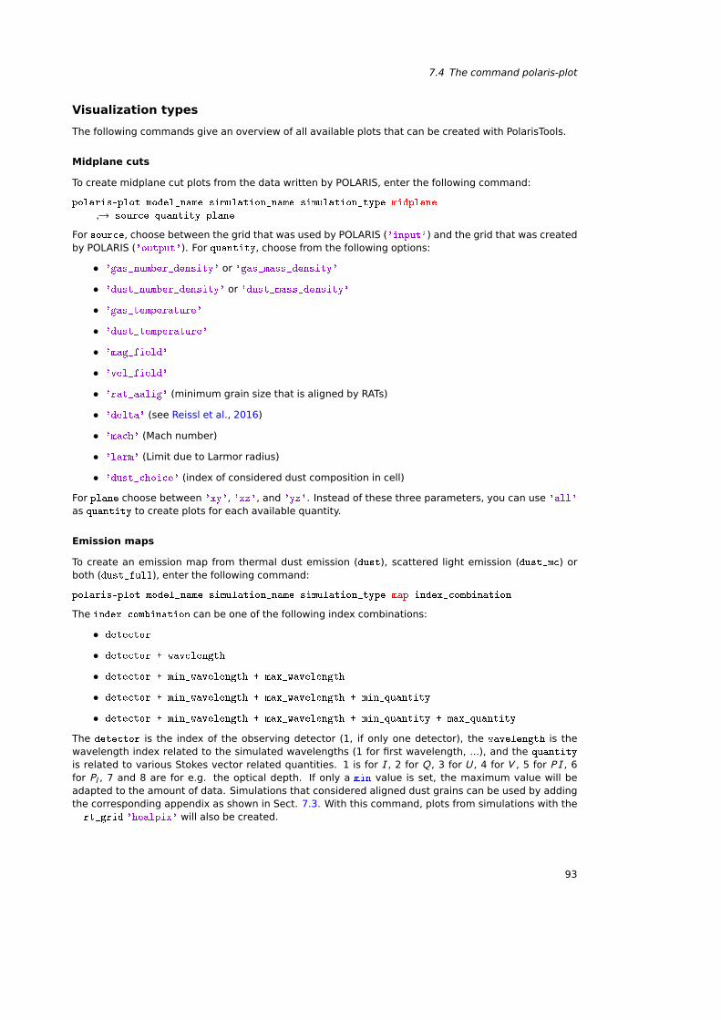
7.4 The command polaris-plot
Visualization types
The following commands give an overview of all available plots that can be created with PolarisTools.
Midplane cuts
To create midplane cut plots from the data written by POLARIS, enter the following command:
polaris-plot model_name simulation_name simulation_type midplane
→ source quantity plane
For source, choose between the grid that was used by POLARIS ('input') and the grid that was createdby POLARIS ('output'). For quantity, choose from the following options:
• 'gas_number_density' or 'gas_mass_density'
• 'dust_number_density' or 'dust_mass_density'
• 'gas_temperature'
• 'dust_temperature'
• 'mag_field'
• 'vel_field'
• 'rat_aalig' (minimum grain size that is aligned by RATs)
• 'delta' (see Reissl et al., 2016)
• 'mach' (Mach number)
• 'larm' (Limit due to Larmor radius)
• 'dust_choice' (index of considered dust composition in cell)
For plane choose between 'xy', 'xz', and 'yz'. Instead of these three parameters, you can use 'all'
as quantity to create plots for each available quantity.
Emission maps
To create an emission map from thermal dust emission (dust), scattered light emission (dust_mc) orboth (dust_full), enter the following command:
polaris-plot model_name simulation_name simulation_type map index_combination
The index_combination can be one of the following index combinations:
• detector
• detector + wavelength
• detector + min_wavelength + max_wavelength
• detector + min_wavelength + max_wavelength + min_quantity
• detector + min_wavelength + max_wavelength + min_quantity + max_quantity
The detector is the index of the observing detector (1, if only one detector), the wavelength is thewavelength index related to the simulated wavelengths (1 for first wavelength, ...), and the quantity
is related to various Stokes vector related quantities. 1 is for I , 2 for Q , 3 for U , 4 for V , 5 for P I , 6for Pl , 7 and 8 are for e.g. the optical depth. If only a min value is set, the maximum value will beadapted to the amount of data. Simulations that considered aligned dust grains can be used by addingthe corresponding appendix as shown in Sect. 7.3. With this command, plots from simulations with the--rt_grid 'healpix' will also be created.
93
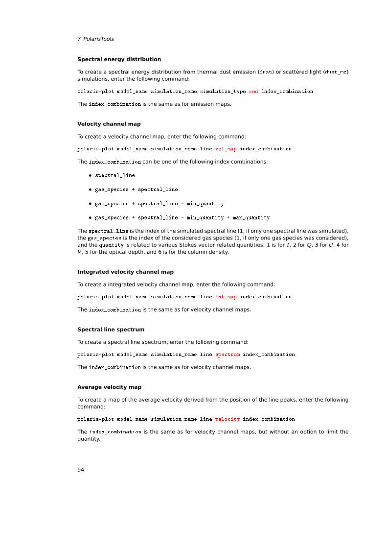
7 PolarisTools
Spectral energy distribution
To create a spectral energy distribution from thermal dust emission (dust) or scattered light (dust_mc)simulations, enter the following command:
polaris-plot model_name simulation_name simulation_type sed index_combination
The index_combination is the same as for emission maps.
Velocity channel map
To create a velocity channel map, enter the following command:
polaris-plot model_name simulation_name line vel_map index_combination
The index_combination can be one of the following index combinations:
• spectral_line
• gas_species + spectral_line
• gas_species + spectral_line + min_quantity
• gas_species + spectral_line + min_quantity + max_quantity
The spectral_line is the index of the simulated spectral line (1, if only one spectral line was simulated),the gas_species is the index of the considered gas species (1, if only one gas species was considered),and the quantity is related to various Stokes vector related quantities. 1 is for I , 2 for Q , 3 for U , 4 forV , 5 for the optical depth, and 6 is for the column density.
Integrated velocity channel map
To create a integrated velocity channel map, enter the following command:
polaris-plot model_name simulation_name line int_map index_combination
The index_combination is the same as for velocity channel maps.
Spectral line spectrum
To create a spectral line spectrum, enter the following command:
polaris-plot model_name simulation_name line spectrum index_combination
The index_combination is the same as for velocity channel maps.
Average velocity map
To create a map of the average velocity derived from the position of the line peaks, enter the followingcommand:
polaris-plot model_name simulation_name line velocity index_combination
The index_combination is the same as for velocity channel maps, but without an option to limit thequantity.
94
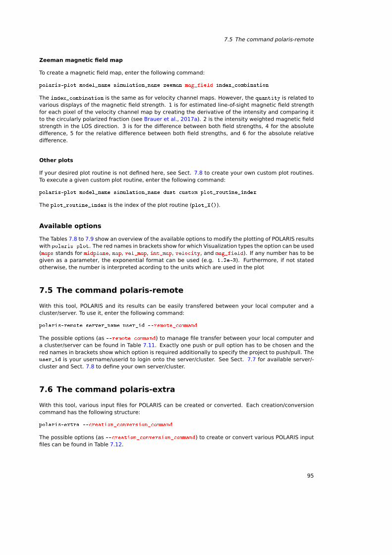
7.5 The command polaris-remote
Zeeman magnetic field map
To create a magnetic field map, enter the following command:
polaris-plot model_name simulation_name zeeman mag_field index_combination
The index_combination is the same as for velocity channel maps. However, the quantity is related tovarious displays of the magnetic field strength. 1 is for estimated line-of-sight magnetic field strengthfor each pixel of the velocity channel map by creating the derivative of the intensity and comparing itto the circularly polarized fraction (see Brauer et al., 2017a). 2 is the intensity weighted magnetic fieldstrength in the LOS direction. 3 is for the difference between both field strengths, 4 for the absolutedifference, 5 for the relative difference between both field strengths, and 6 for the absolute relativedifference.
Other plots
If your desired plot routine is not defined here, see Sect. 7.8 to create your own custom plot routines.To execute a given custom plot routine, enter the following command:
polaris-plot model_name simulation_name dust custom plot_routine_index
The plot_routine_index is the index of the plot routine (plot_X()).
Available options
The Tables 7.8 to 7.9 show an overview of the available options to modify the plotting of POLARIS resultswith polaris-plot. The red names in brackets show for which Visualization types the option can be used(maps stands for midplane, map, vel_map, int_map, velocity, and mag_field). If any number has to begiven as a parameter, the exponential format can be used (e.g. 1.2e-3). Furthermore, if not statedotherwise, the number is interpreted acording to the units which are used in the plot
7.5 The command polaris-remote
With this tool, POLARIS and its results can be easily transfered between your local computer and acluster/server. To use it, enter the following command:
polaris-remote server_name user_id --remote_command
The possible options (as --remote_command) to manage file transfer between your local computer anda cluster/server can be found in Table 7.11. Exactly one push or pull option has to be chosen and thered names in brackets show which option is required additionally to specify the project to push/pull. Theuser_id is your username/userid to login onto the server/cluster. See Sect. 7.7 for available server/-cluster and Sect. 7.8 to define your own server/cluster.
7.6 The command polaris-extra
With this tool, various input files for POLARIS can be created or converted. Each creation/conversioncommand has the following structure:
polaris-extra --creation_conversion_command
The possible options (as --creation_conversion_command) to create or convert various POLARIS inputfiles can be found in Table 7.12.
95
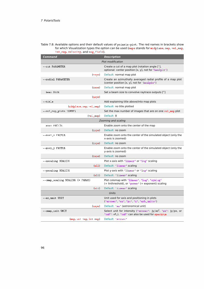
7 PolarisTools
Table 7.8: Available options and their default values of polaris-plot. The red names in brackets showfor which Visualization types the option can be used (maps stands for midplane, map, vel_map,int_map, velocity, and mag_field).
Command Description
Plot modification
--cut PARAMETER Create a cut of a map plot (rotation angle [],optional: center position [x, y], not for 'healpix')
(maps) Default: normal map plot
--radial PARAMETER Create an azimuthally averaged radial profile of a map plot(center position [x, y], not for 'healpix')
(maps) Default: normal map plot
--beam SIZE Set a beam size to convolve raytrace outputs [′′]
(maps)
--title Add explaining title above/into map plots
(midplane, map, vel_map) Default: no title plotted
--vel_map_plots NUMBER Set the max number of images that are on one vel_map plot
(vel_map) Default: 8
Zooming and scaling
--zoom FACTOR Enable zoom onto the center of the map
(maps) Default: no zoom
--zoom_x FACTOR Enable zoom onto the center of the simulated object (only thex-axis is zoomed)
(maps) Default: no zoom
--zoom_y FACTOR Enable zoom onto the center of the simulated object (only they-axis is zoomed)
(maps) Default: no zoom
--xscaling SCALING Plot x-axis with 'linear' or 'log' scaling
(all) Default: 'linear' scaling
--yscaling SCALING Plot y-axis with 'linear' or 'log' scaling
(all) Default: 'linear' scaling
--cmap_scaling SCALING (+ PARAM) Plot colomap with 'linear', 'log', 'symlog'(+ linthreshold), or 'power' (+ exponent) scaling
(all) Default: 'linear' scaling
Units
--ax_unit UNIT Unit used for axis and positioning in plots('arcsec', 'au', 'pc', 'm', 'arb_units')
(maps) Default: 'au' (astronomical unit)
--cmap_unit UNIT Select unit for intensity ('arcsec': Jy/as2, 'px': Jy/px, or'nuF': νFν). 'nuF' can also be used for spectrum
(map, vel_map, int_map) Default: 'arcsec'
96
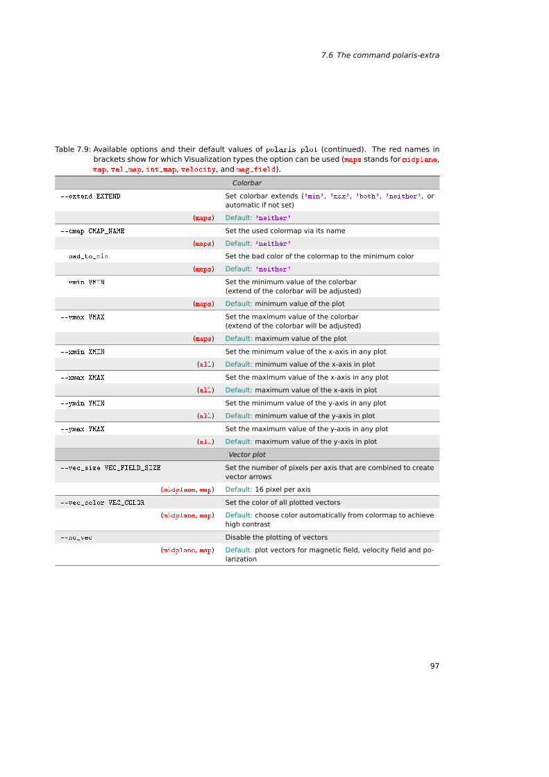
7.6 The command polaris-extra
Table 7.9: Available options and their default values of polaris-plot (continued). The red names inbrackets show for which Visualization types the option can be used (maps stands for midplane,map, vel_map, int_map, velocity, and mag_field).
Colorbar
--extend EXTEND Set colorbar extends ('min', 'max', 'both', 'neither', orautomatic if not set)
(maps) Default: 'neither'
--cmap CMAP_NAME Set the used colormap via its name
(maps) Default: 'neither'
--bad_to_min Set the bad color of the colormap to the minimum color
(maps) Default: 'neither'
--vmin VMIN Set the minimum value of the colorbar(extend of the colorbar will be adjusted)
(maps) Default: minimum value of the plot
--vmax VMAX Set the maximum value of the colorbar(extend of the colorbar will be adjusted)
(maps) Default: maximum value of the plot
--xmin XMIN Set the minimum value of the x-axis in any plot
(all) Default: minimum value of the x-axis in plot
--xmax XMAX Set the maximum value of the x-axis in any plot
(all) Default: maximum value of the x-axis in plot
--ymin YMIN Set the minimum value of the y-axis in any plot
(all) Default: minimum value of the y-axis in plot
--ymax YMAX Set the maximum value of the y-axis in any plot
(all) Default: maximum value of the y-axis in plot
Vector plot
--vec_size VEC_FIELD_SIZE Set the number of pixels per axis that are combined to createvector arrows
(midplane, map) Default: 16 pixel per axis
--vec_color VEC_COLOR Set the color of all plotted vectors
(midplane, map) Default: choose color automatically from colormap to achievehigh contrast
--no_vec Disable the plotting of vectors
(midplane, map) Default: plot vectors for magnetic field, velocity field and po-larization
97
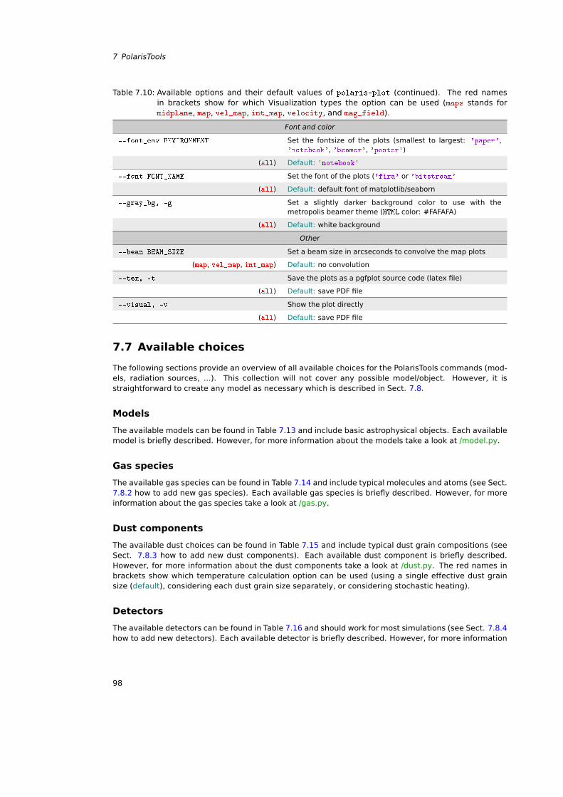
7 PolarisTools
Table 7.10: Available options and their default values of polaris-plot (continued). The red namesin brackets show for which Visualization types the option can be used (maps stands formidplane, map, vel_map, int_map, velocity, and mag_field).
Font and color
--font_env ENVIRONMENT Set the fontsize of the plots (smallest to largest: 'paper','notebook', 'beamer', 'poster')
(all) Default: 'notebook'
--font FONT_NAME Set the font of the plots ('fira' or 'bitstream'
(all) Default: default font of matplotlib/seaborn
--gray_bg, -g Set a slightly darker background color to use with themetropolis beamer theme (HTML color: #FAFAFA)
(all) Default: white background
Other
--beam BEAM_SIZE Set a beam size in arcseconds to convolve the map plots
(map, vel_map, int_map) Default: no convolution
--tex, -t Save the plots as a pgfplot source code (latex file)
(all) Default: save PDF file
--visual, -v Show the plot directly
(all) Default: save PDF file
7.7 Available choices
The following sections provide an overview of all available choices for the PolarisTools commands (mod-els, radiation sources, ...). This collection will not cover any possible model/object. However, it isstraightforward to create any model as necessary which is described in Sect. 7.8.
Models
The available models can be found in Table 7.13 and include basic astrophysical objects. Each availablemodel is briefly described. However, for more information about the models take a look at /model.py.
Gas species
The available gas species can be found in Table 7.14 and include typical molecules and atoms (see Sect.7.8.2 how to add new gas species). Each available gas species is briefly described. However, for moreinformation about the gas species take a look at /gas.py.
Dust components
The available dust choices can be found in Table 7.15 and include typical dust grain compositions (seeSect. 7.8.3 how to add new dust components). Each available dust component is briefly described.However, for more information about the dust components take a look at /dust.py. The red names inbrackets show which temperature calculation option can be used (using a single effective dust grainsize (default), considering each dust grain size separately, or considering stochastic heating).
Detectors
The available detectors can be found in Table 7.16 and should work for most simulations (see Sect. 7.8.4how to add new detectors). Each available detector is briefly described. However, for more information
98
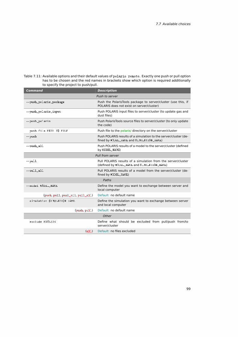
7.7 Available choices
Table 7.11: Available options and their default values of polaris-remote. Exactly one push or pull optionhas to be chosen and the red names in brackets show which option is required additionallyto specify the project to push/pull.
Command Description
Push to server
--push_polaris_package Push the PolarisTools package to server/cluster (use this, ifPOLARIS does not exist on server/cluster)
--push_polaris_input Push POLARIS input files to server/cluster (to update gas anddust files)
--push_polaris Push PolarisTools source files to server/cluster (to only updatethe code)
--push_file PATH_TO_FILE Push file to the polaris/ directory on the server/cluster
--push Push POLARIS results of a simulation to the server/cluster (de-fined by MODEL_NAME and SIMULATION_NAME)
--push_all Push POLARIS results of a model to the server/cluster (definedby MODEL_NAME)
Pull from server
--pull Pull POLARIS results of a simulation from the server/cluster(defined by MODEL_NAME and SIMULATION_NAME)
--pull_all Pull POLARIS results of a model from the server/cluster (de-fined by MODEL_NAME)
Paths
--model MODEL_NAME Define the model you want to exchange between server andlocal computer
(push, pull, push_all, pull_all) Default: no default name
--simulation SIMULATION_NAME Define the simulation you want to exchange between serverand local computer
(push, pull) Default: no default name
Other
--exclude EXCLUDE Define what should be excluded from pull/push from/toserver/cluster
(all) Default: no files excluded
99
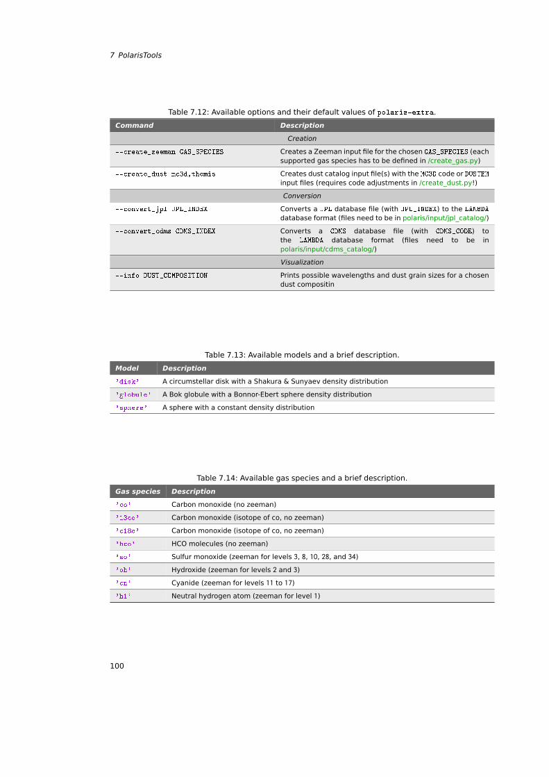
7 PolarisTools
Table 7.12: Available options and their default values of polaris-extra.
Command Description
Creation
--create_zeeman GAS_SPECIES Creates a Zeeman input file for the chosen GAS_SPECIES (eachsupported gas species has to be defined in /create_gas.py)
--create_dust mc3d,themis Creates dust catalog input file(s) with the MC3D code or DUSTEMinput files (requires code adjustments in /create_dust.py!)
Conversion
--convert_jpl JPL_INDEX Converts a JPL database file (with JPL_INDEX) to the LAMBDA
database format (files need to be in polaris/input/jpl_catalog/)
--convert_cdms CDMS_INDEX Converts a CDMS database file (with CDMS_CODE) tothe LAMBDA database format (files need to be inpolaris/input/cdms_catalog/)
Visualization
--info DUST_COMPOSITION Prints possible wavelengths and dust grain sizes for a chosendust compositin
Table 7.13: Available models and a brief description.
Model Description
'disk' A circumstellar disk with a Shakura & Sunyaev density distribution
'globule' A Bok globule with a Bonnor-Ebert sphere density distribution
'sphere' A sphere with a constant density distribution
Table 7.14: Available gas species and a brief description.
Gas species Description
'co' Carbon monoxide (no zeeman)
'13co' Carbon monoxide (isotope of co, no zeeman)
'c18o' Carbon monoxide (isotope of co, no zeeman)
'hco' HCO molecules (no zeeman)
'so' Sulfur monoxide (zeeman for levels 3, 8, 10, 28, and 34)
'oh' Hydroxide (zeeman for levels 2 and 3)
'cn' Cyanide (zeeman for levels 11 to 17)
'h1' Neutral hydrogen atom (zeeman for level 1)
100
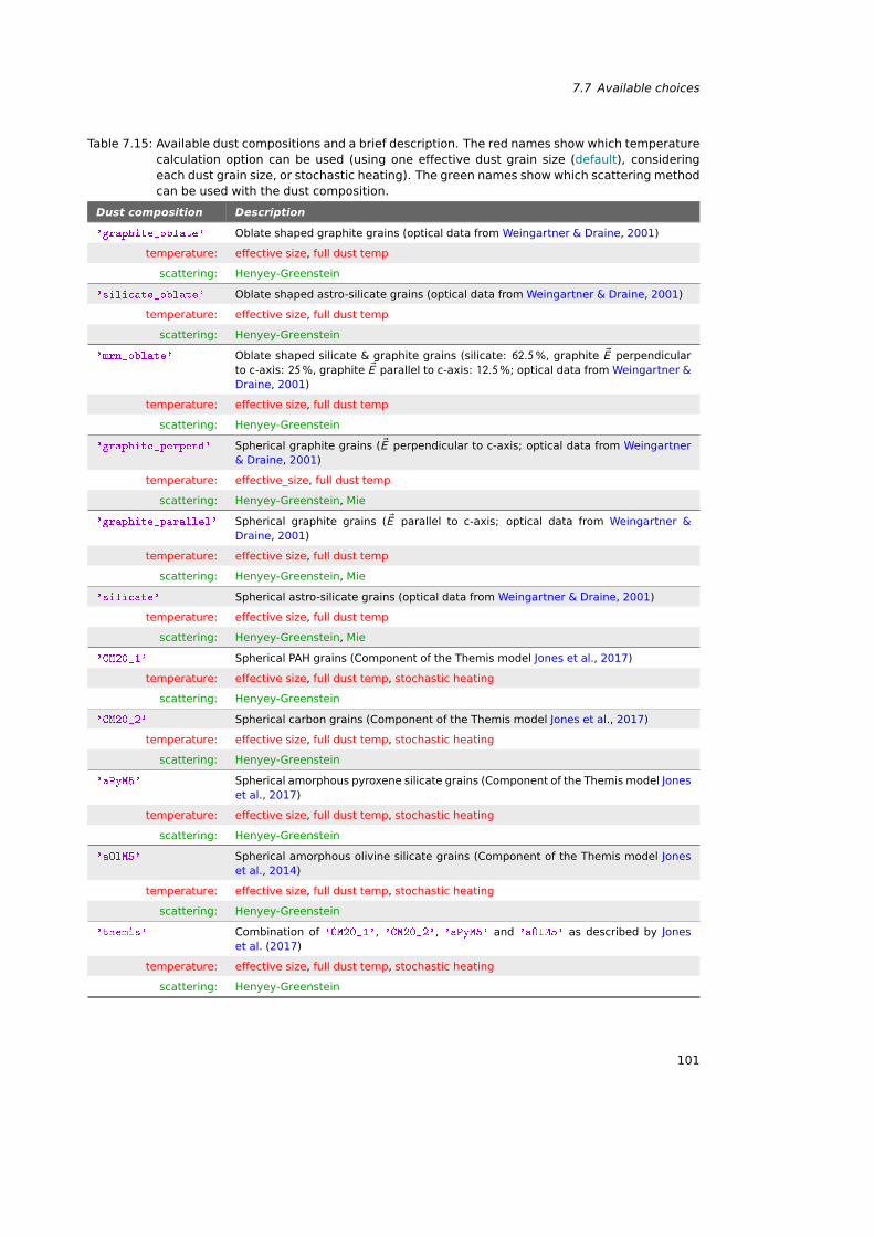
7.7 Available choices
Table 7.15: Available dust compositions and a brief description. The red names show which temperaturecalculation option can be used (using one effective dust grain size (default), consideringeach dust grain size, or stochastic heating). The green names show which scattering methodcan be used with the dust composition.
Dust composition Description
'graphite_oblate' Oblate shaped graphite grains (optical data from Weingartner & Draine, 2001)
temperature: effective size, full dust temp
scattering: Henyey-Greenstein
'silicate_oblate' Oblate shaped astro-silicate grains (optical data from Weingartner & Draine, 2001)
temperature: effective size, full dust temp
scattering: Henyey-Greenstein
'mrn_oblate' Oblate shaped silicate & graphite grains (silicate: 62.5%, graphite ®E perpendicularto c-axis: 25%, graphite ®E parallel to c-axis: 12.5%; optical data from Weingartner &Draine, 2001)
temperature: effective size, full dust temp
scattering: Henyey-Greenstein
'graphite_perpend' Spherical graphite grains ( ®E perpendicular to c-axis; optical data from Weingartner& Draine, 2001)
temperature: effective_size, full dust temp
scattering: Henyey-Greenstein, Mie
'graphite_parallel' Spherical graphite grains ( ®E parallel to c-axis; optical data from Weingartner &Draine, 2001)
temperature: effective size, full dust temp
scattering: Henyey-Greenstein, Mie
'silicate' Spherical astro-silicate grains (optical data from Weingartner & Draine, 2001)
temperature: effective size, full dust temp
scattering: Henyey-Greenstein, Mie
'CM20_1' Spherical PAH grains (Component of the Themis model Jones et al., 2017)
temperature: effective size, full dust temp, stochastic heating
scattering: Henyey-Greenstein
'CM20_2' Spherical carbon grains (Component of the Themis model Jones et al., 2017)
temperature: effective size, full dust temp, stochastic heating
scattering: Henyey-Greenstein
'aPyM5' Spherical amorphous pyroxene silicate grains (Component of the Themis model Joneset al., 2017)
temperature: effective size, full dust temp, stochastic heating
scattering: Henyey-Greenstein
'aOlM5' Spherical amorphous olivine silicate grains (Component of the Themis model Joneset al., 2014)
temperature: effective size, full dust temp, stochastic heating
scattering: Henyey-Greenstein
'themis' Combination of 'CM20_1', 'CM20_2', 'aPyM5' and 'aOlM5' as described by Joneset al. (2017)
temperature: effective size, full dust temp, stochastic heating
scattering: Henyey-Greenstein
101
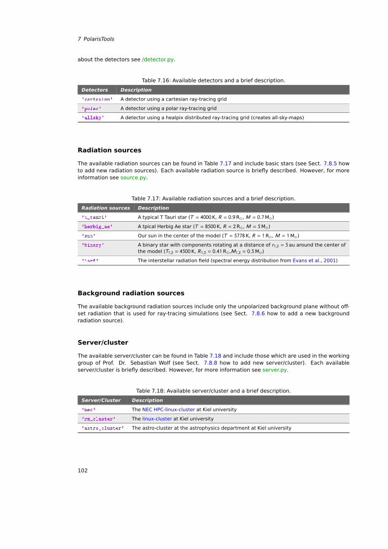
7 PolarisTools
about the detectors see /detector.py.
Table 7.16: Available detectors and a brief description.
Detectors Description
'cartesian' A detector using a cartesian ray-tracing grid
'polar' A detector using a polar ray-tracing grid
'allsky' A detector using a healpix distributed ray-tracing grid (creates all-sky-maps)
Radiation sources
The available radiation sources can be found in Table 7.17 and include basic stars (see Sect. 7.8.5 howto add new radiation sources). Each available radiation source is briefly described. However, for moreinformation see source.py.
Table 7.17: Available radiation sources and a brief description.
Radiation sources Description
't_tauri' A typical T Tauri star (T = 4000K, R = 0.9R, M = 0.7M)
'herbig_ae' A tpical Herbig Ae star (T = 8500K, R = 2R, M = 5M)
'sun' Our sun in the center of the model (T = 5778K, R = 1R, M = 1M)
'binary' A binary star with components rotating at a distance of r1,2 = 5 au around the center ofthe model (T1,2 = 4500K, R1,2 = 0.41R,M1,2 = 0.5M)
'isrf' The interstellar radiation field (spectral energy distribution from Evans et al., 2001)
Background radiation sources
The available background radiation sources include only the unpolarized background plane without off-set radiation that is used for ray-tracing simulations (see Sect. 7.8.6 how to add a new backgroundradiation source).
Server/cluster
The available server/cluster can be found in Table 7.18 and include those which are used in the workinggroup of Prof. Dr. Sebastian Wolf (see Sect. 7.8.8 how to add new server/cluster). Each availableserver/cluster is briefly described. However, for more information see server.py.
Table 7.18: Available server/cluster and a brief description.
Server/Cluster Description
'nec' The NEC HPC-linux-cluster at Kiel university
'rz_cluster' The linux-cluster at Kiel university
'astro_cluster' The astro-cluster at the astrophysics department at Kiel university
102
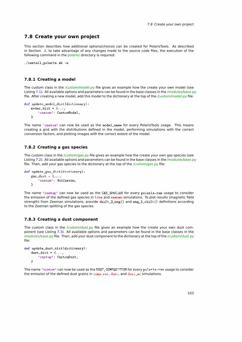
7.8 Create your own project
7.8 Create your own project
This section describes how additional options/choices can be created for PolarisTools. As describedin Section. 2, to take advantage of any changes made to the source code files, the execution of thefollowing command in the polaris/ directory is required:
./install_polaris.sh -u
7.8.1 Creating a model
The custom class in the /custom/model.py file gives an example how the create your own model (seeListing 7.1). All available options and parameters can be found in the base classes in the /modules/base.pyfile. After creating a new model, add this model to the dictionary at the top of the /custom/model.py file:
def update_model_dict(dictionary):
model_dict = ...,
'custom': CustomModel,
The name 'custom' can now be used as the model_name for every PolarisTools usage. This meanscreating a grid with the distributions defined in the model, performing simulations with the correctconversion factors, and plotting images with the correct extent of the model.
7.8.2 Creating a gas species
The custom class in the /custom/gas.py file gives an example how the create your own gas species (seeListing 7.2). All available options and parameters can be found in the base classes in the /modules/base.pyfile. Then, add your gas species to the dictionary at the top of the /custom/gas.py file:
def update_gas_dict(dictionary):
gas_dict = ...,
'custom': MolCustom,
The name 'custom' can now be used as the GAS_SPECIES for every polaris-run usage to considerthe emission of the defined gas species in line and zeeman simulations. To plot results (magnetic fieldstrength) from Zeeman simulations, provide shift_2_mag() and mag_2_shift() definitions accordingto the Zeeman splitting of the gas species.
7.8.3 Creating a dust component
The custom class in the /custom/dust.py file gives an example how the create your own dust com-ponent (see Listing 7.3). All available options and parameters can be found in the base classes in the/modules/base.py file. Then, add your dust component to the dictionary at the top of the /custom/dust.pyfile:
def update_dust_dict(dictionary):
dust_dict = ...,
'custom': CustomDust,
The name 'custom' can now be used as the DUST_COMPOSITION for every polaris-run usage to considerthe emission of the defined dust grains in temp, rat, dust, and dust_mc simulations.
103
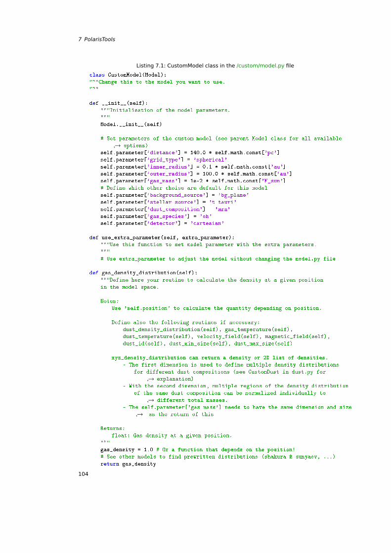
7 PolarisTools
Listing 7.1: CustomModel class in the /custom/model.py file
class CustomModel(Model):
"""Change this to the model you want to use.
"""
def __init__(self):
"""Initialisation of the model parameters.
"""
Model.__init__(self)
# Set parameters of the custom model (see parent Model class for all available
→ options)
self.parameter['distance'] = 140.0 * self.math.const['pc']
self.parameter['grid_type'] = 'spherical'
self.parameter['inner_radius'] = 0.1 * self.math.const['au']
self.parameter['outer_radius'] = 100.0 * self.math.const['au']
self.parameter['gas_mass'] = 1e-2 * self.math.const['M_sun']
# Define which other choise are default for this model
self.parameter['background_source'] = 'bg_plane'
self.parameter['stellar_source'] = 't_tauri'
self.parameter['dust_composition'] = 'mrn'
self.parameter['gas_species'] = 'oh'
self.parameter['detector'] = 'cartesian'
def use_extra_parameter(self, extra_parameter):
"""Use this function to set model parameter with the extra parameters.
"""
# Use extra_parameter to adjust the model without changing the model.py file
def gas_density_distribution(self):
"""Define here your routine to calculate the density at a given position
in the model space.
Notes:
Use 'self.position' to calculate the quantity depending on position.
Define also the following routines if necessary:
dust_density_distribution(self), gas_temperature(self),
dust_temperature(self), velocity_field(self), magnetic_field(self),
dust_id(self), dust_min_size(self), dust_max_size(self)
xyz_density_distribution can return a density or 2D list of densities.
- The first dimension is used to define multiple density distributions
for different dust compositions (see CustomDust in dust.py for
→ explanation)
- With the second dimension, multiple regions of the density distribution
of the same dust composition can be normalized individually to
→ different total masses.
- The self.parameter['gas_mass'] needs to have the same dimension and size
→ as the return of this
Returns:
float: Gas density at a given position.
"""
gas_density = 1.0 # Or a function that depends on the position!
# See other models to find prewritten distributions (shakura & sunyaev, ...)
return gas_density
104
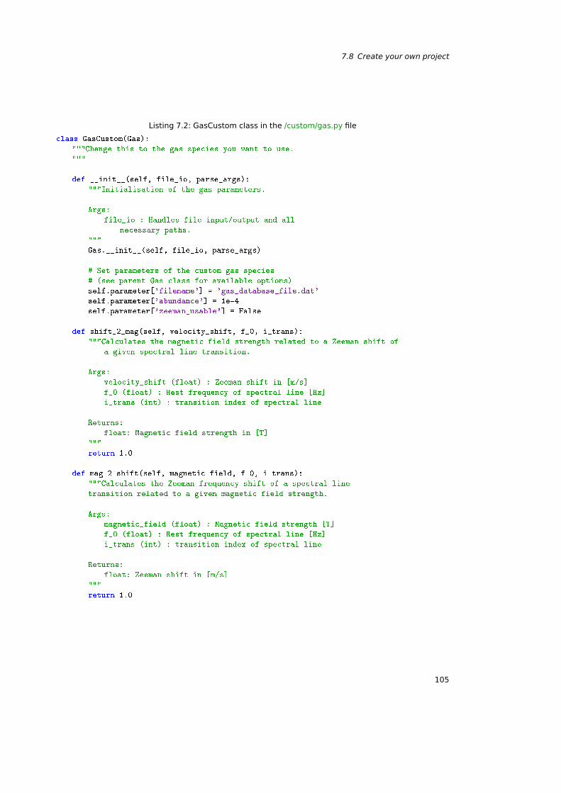
7.8 Create your own project
Listing 7.2: GasCustom class in the /custom/gas.py file
class GasCustom(Gas):
"""Change this to the gas species you want to use.
"""
def __init__(self, file_io, parse_args):
"""Initialisation of the gas parameters.
Args:
file_io : Handles file input/output and all
necessary paths.
"""
Gas.__init__(self, file_io, parse_args)
# Set parameters of the custom gas species
# (see parent Gas class for available options)
self.parameter['filename'] = 'gas_database_file.dat'
self.parameter['abundance'] = 1e-4
self.parameter['zeeman_usable'] = False
def shift_2_mag(self, velocity_shift, f_0, i_trans):
"""Calculates the magnetic field strength related to a Zeeman shift of
a given spectral line transition.
Args:
velocity_shift (float) : Zeeman shift in [m/s]
f_0 (float) : Rest frequency of spectral line [Hz]
i_trans (int) : transition index of spectral line
Returns:
float: Magnetic field strength in [T]
"""
return 1.0
def mag_2_shift(self, magnetic_field, f_0, i_trans):
"""Calculates the Zeeman frequency shift of a spectral line
transition related to a given magnetic field strength.
Args:
magnetic_field (float) : Magnetic field strength [T]
f_0 (float) : Rest frequency of spectral line [Hz]
i_trans (int) : transition index of spectral line
Returns:
float: Zeeman shift in [m/s]
"""
return 1.0
105
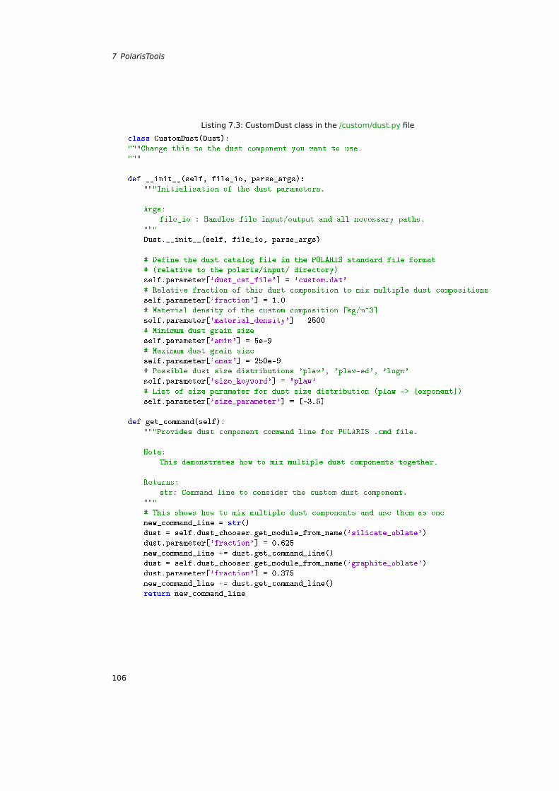
7 PolarisTools
Listing 7.3: CustomDust class in the /custom/dust.py file
class CustomDust(Dust):
"""Change this to the dust component you want to use.
"""
def __init__(self, file_io, parse_args):
"""Initialisation of the dust parameters.
Args:
file_io : Handles file input/output and all necessary paths.
"""
Dust.__init__(self, file_io, parse_args)
# Define the dust catalog file in the POLARIS standard file format
# (relative to the polaris/input/ directory)
self.parameter['dust_cat_file'] = 'custom.dat'
# Relative fraction of this dust composition to mix multiple dust compositions
self.parameter['fraction'] = 1.0
# Material density of the custom composition [kg/m^3]
self.parameter['material_density'] = 2500
# Minimum dust grain size
self.parameter['amin'] = 5e-9
# Maximum dust grain size
self.parameter['amax'] = 250e-9
# Possible dust size distributions 'plaw', 'plaw-ed', 'logn'
self.parameter['size_keyword'] = 'plaw'
# List of size parameter for dust size distribution (plaw -> [exponent])
self.parameter['size_parameter'] = [-3.5]
def get_command(self):
"""Provides dust component command line for POLARIS .cmd file.
Note:
This demonstrates how to mix multiple dust components together.
Returns:
str: Command line to consider the custom dust component.
"""
# This shows how to mix multiple dust components and use them as one
new_command_line = str()
dust = self.dust_chooser.get_module_from_name('silicate_oblate')
dust.parameter['fraction'] = 0.625
new_command_line += dust.get_command_line()
dust = self.dust_chooser.get_module_from_name('graphite_oblate')
dust.parameter['fraction'] = 0.375
new_command_line += dust.get_command_line()
return new_command_line
106
7.8 Create your own project
7.8.4 Creating a detector
The custom class in the /custom/detector.py file gives an example how the create your own detector(see Listing 7.4 and 7.5). All available options and parameters can be found in the base classes in the/modules/base.py file.
Then, add your detector to the dictionary at the top of the /custom/detector.py file:
def update_detector_dict(dictionary):
detector_dict = ...,
'custom': CustomDetector,
The name 'custom' can now be used as the DETECTOR for every polaris-run usage to consider observethe emission in dust, dust_mc, and line simulations.
7.8.5 Creating a stellar radiation source
The custom class in the /custom/source.py file gives an example how the create your own stellar radi-ation source (see Listing 7.6). All available options and parameters can be found in the base classesin the /modules/base.py file. Then, add your stellar radiation source to the dictionary at the top of the/custom/source.py file:
def update_sources_dict(dictionary):
sources_dict = ...,
'custom': CustomStar,
The name 'custom' can now be used as the RADIATION_SOURCE for every polaris-run usage to considerthe emission of the defined stellar radiation source in temp, rat, and dust_mc simulations.
7.8.6 Creating a background radiation source
The custom class in the /custom/bg_source.py file gives an example how the create your own back-ground radiation source (see Listing 7.7). All available options and parameters can be found in the baseclasses in the /modules/base.py file. Then, add your background radiation source to the dictionary atthe top of the /custom/bg_source.py file:
def update_bg_source_dict(dictionary):
bg_source_dict = ...,
'custom': CustomBGsource,
The name 'custom' can now be used as the BG_SOURCE for every polaris-run usage to consider theemission of the defined background radiation source in dust and line simulations (ray-tracing).
7.8.7 Creating a custom plot routine
The custom function in the /custom/plots.py file gives an example how the create your own plottingroutines (see Listing 7.8). Perform a custom plotting routine by executing the following command:
polaris-plot model_name simulation_name simulation_type custom X
The number X is the unique identifier for the custom plot routine plot_X().
107
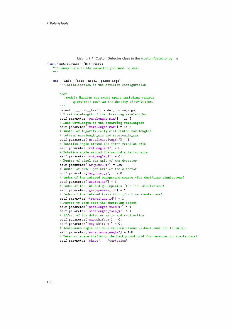
7 PolarisTools
Listing 7.4: CustomDetector class in the /custom/detector.py file
class CustomDetector(Detector):
"""Change this to the detector you want to use.
"""
def __init__(self, model, parse_args):
"""Initialisation of the detector configuration.
Args:
model: Handles the model space including various
quantities such as the density distribution.
"""
Detector.__init__(self, model, parse_args)
# First wavelength of the observing wavelengths
self.parameter['wavelength_min'] = 1e-6
# Last wavelength of the observing wavelengths
self.parameter['wavelength_max'] = 1e-6
# Number of logaritmically distributed wavelengths
# between wavelength_min and wavelength_max
self.parameter['nr_of_wavelength'] = 1
# Rotation angle around the first rotation axis
self.parameter['rot_angle_1'] = 0.
# Rotation angle around the second rotation axis
self.parameter['rot_angle_2'] = 0.
# Number of pixel per axis of the detector
self.parameter['nr_pixel_x'] = 256
# Number of pixel per axis of the detector
self.parameter['nr_pixel_y'] = 256
# Index of the related background source (for dust/line simulations)
self.parameter['source_id'] = 1
# Index of the related gas_species (for line simulations)
self.parameter['gas_species_id'] = 1
# Index of the related transition (for line simulations)
self.parameter['transition_id'] = 1
# Factor to zoom onto the observing object
self.parameter['sidelength_zoom_x'] = 1
self.parameter['sidelength_zoom_y'] = 1
# Offset of the detector in x- and y-direction
self.parameter['map_shift_x'] = 0.
self.parameter['map_shift_y'] = 0.
# Acceptance angle for dust_mc simulations without peel-off technique
self.parameter['acceptance_angle'] = 1.0
# Detector shape (defining the background grid for ray-tracing simulations)
self.parameter['shape'] = 'cartesian'
108
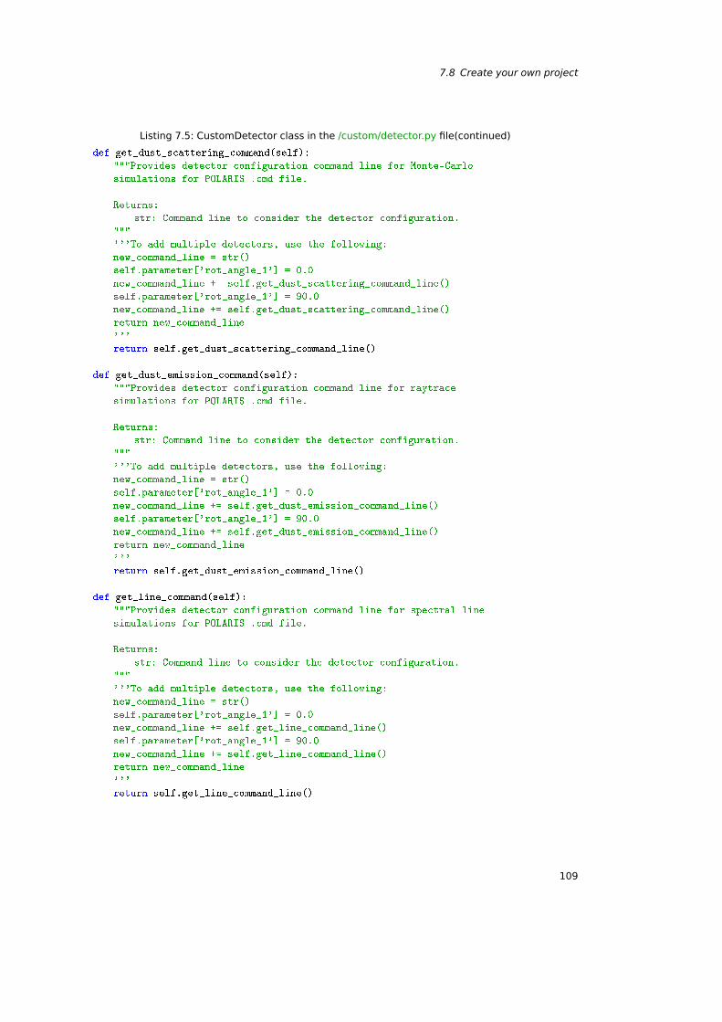
7.8 Create your own project
Listing 7.5: CustomDetector class in the /custom/detector.py file(continued)
def get_dust_scattering_command(self):
"""Provides detector configuration command line for Monte-Carlo
simulations for POLARIS .cmd file.
Returns:
str: Command line to consider the detector configuration.
"""
'''To add multiple detectors, use the following:
new_command_line = str()
self.parameter['rot_angle_1'] = 0.0
new_command_line += self.get_dust_scattering_command_line()
self.parameter['rot_angle_1'] = 90.0
new_command_line += self.get_dust_scattering_command_line()
return new_command_line
'''
return self.get_dust_scattering_command_line()
def get_dust_emission_command(self):
"""Provides detector configuration command line for raytrace
simulations for POLARIS .cmd file.
Returns:
str: Command line to consider the detector configuration.
"""
'''To add multiple detectors, use the following:
new_command_line = str()
self.parameter['rot_angle_1'] = 0.0
new_command_line += self.get_dust_emission_command_line()
self.parameter['rot_angle_1'] = 90.0
new_command_line += self.get_dust_emission_command_line()
return new_command_line
'''
return self.get_dust_emission_command_line()
def get_line_command(self):
"""Provides detector configuration command line for spectral line
simulations for POLARIS .cmd file.
Returns:
str: Command line to consider the detector configuration.
"""
'''To add multiple detectors, use the following:
new_command_line = str()
self.parameter['rot_angle_1'] = 0.0
new_command_line += self.get_line_command_line()
self.parameter['rot_angle_1'] = 90.0
new_command_line += self.get_line_command_line()
return new_command_line
'''
return self.get_line_command_line()
109
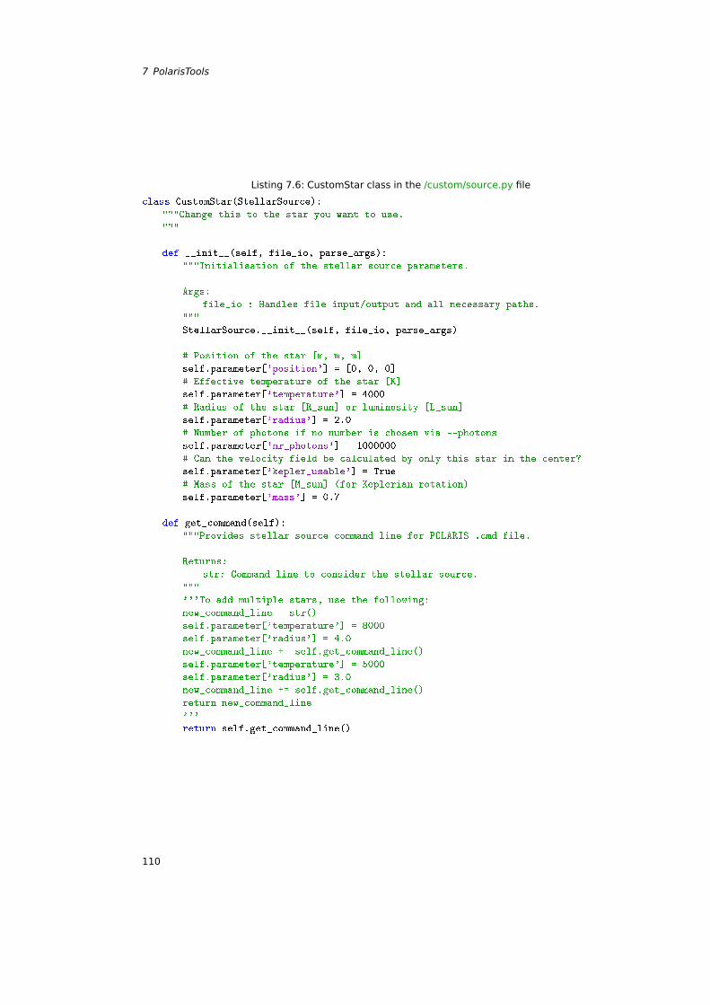
7 PolarisTools
Listing 7.6: CustomStar class in the /custom/source.py file
class CustomStar(StellarSource):
"""Change this to the star you want to use.
"""
def __init__(self, file_io, parse_args):
"""Initialisation of the stellar source parameters.
Args:
file_io : Handles file input/output and all necessary paths.
"""
StellarSource.__init__(self, file_io, parse_args)
# Position of the star [m, m, m]
self.parameter['position'] = [0, 0, 0]
# Effective temperature of the star [K]
self.parameter['temperature'] = 4000
# Radius of the star [R_sun] or luminosity [L_sun]
self.parameter['radius'] = 2.0
# Number of photons if no number is chosen via --photons
self.parameter['nr_photons'] = 1000000
# Can the velocity field be calculated by only this star in the center?
self.parameter['kepler_usable'] = True
# Mass of the star [M_sun] (for Keplerian rotation)
self.parameter['mass'] = 0.7
def get_command(self):
"""Provides stellar source command line for POLARIS .cmd file.
Returns:
str: Command line to consider the stellar source.
"""
'''To add multiple stars, use the following:
new_command_line = str()
self.parameter['temperature'] = 8000
self.parameter['radius'] = 4.0
new_command_line += self.get_command_line()
self.parameter['temperature'] = 5000
self.parameter['radius'] = 3.0
new_command_line += self.get_command_line()
return new_command_line
'''
return self.get_command_line()
110
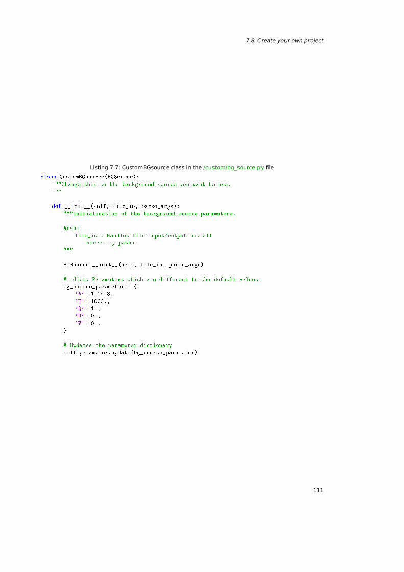
7.8 Create your own project
Listing 7.7: CustomBGsource class in the /custom/bg_source.py file
class CustomBGsource(BGSource):
"""Change this to the background source you want to use.
"""
def __init__(self, file_io, parse_args):
"""Initialisation of the background source parameters.
Args:
file_io : Handles file input/output and all
necessary paths.
"""
BGSource.__init__(self, file_io, parse_args)
#: dict: Parameters which are different to the default values
bg_source_parameter =
'A': 1.0e-3,
'T': 1000.,
'Q': 1.,
'U': 0.,
'V': 0.,
# Updates the parameter dictionary
self.parameter.update(bg_source_parameter)
111
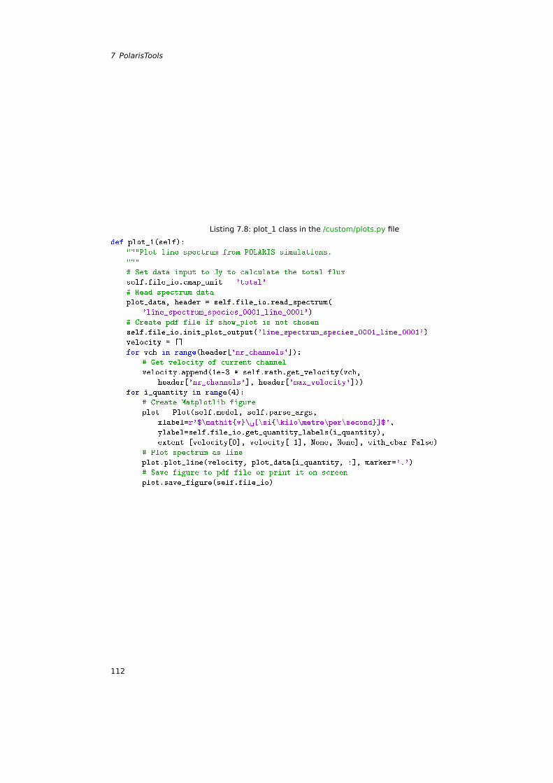
7 PolarisTools
Listing 7.8: plot_1 class in the /custom/plots.py file
def plot_1(self):
"""Plot line spectrum from POLARIS simulations.
"""
# Set data input to Jy to calculate the total flux
self.file_io.cmap_unit = 'total'
# Read spectrum data
plot_data, header = self.file_io.read_spectrum(
'line_spectrum_species_0001_line_0001')
# Create pdf file if show_plot is not chosen
self.file_io.init_plot_output('line_spectrum_species_0001_line_0001')
velocity = []
for vch in range(header['nr_channels']):
# Get velocity of current channel
velocity.append(1e-3 * self.math.get_velocity(vch,
header['nr_channels'], header['max_velocity']))
for i_quantity in range(4):
# Create Matplotlib figure
plot = Plot(self.model, self.parse_args,
xlabel=r'$\mathitv\ [\si\kilo\metre\per\second]$',
ylabel=self.file_io.get_quantity_labels(i_quantity),
extent=[velocity[0], velocity[-1], None, None], with_cbar=False)
# Plot spectrum as line
plot.plot_line(velocity, plot_data[i_quantity, :], marker='.')
# Save figure to pdf file or print it on screen
plot.save_figure(self.file_io)
112
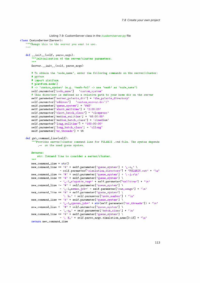
7.8 Create your own project
Listing 7.9: CustomServer class in the /custom/server.py file
class CustomServer(Server):
"""Change this to the server you want to use.
"""
def __init__(self, parse_args):
"""Initialisation of the server/cluster parameters.
"""
Server.__init__(self, parse_args)
# To obtain the 'node_name', enter the following commands on the server/cluster:
# python
# import platform
# platform.node()
# -> 'custom_system' (e.g. 'nesh-fe2' -> use 'nesh' as 'node_name')
self.parameter['node_name'] = 'custom_system'
# This directory is defined as a relative path to your home dir on the server
self.parameter['server_polaris_dir'] = 'the_polaris_directory'
self.parameter['address'] = 'custom_server.de:~/'
self.parameter['queue_system'] = 'PBS'
self.parameter['short_walltime'] = '2:00:00'
self.parameter['short_batch_class'] = 'clexpress'
self.parameter['medium_walltime'] = '48:00:00'
self.parameter['medium_batch_class'] = 'clmedium'
self.parameter['long_walltime'] = '100:00:00'
self.parameter['long_batch_class'] = 'cllong'
self.parameter['nr_threads'] = 16
def get_command_line(self):
"""Provides server/cluster command line for POLARIS .cmd file. The syntax depends
→ on the used queue system.
Returns:
str: Command line to consider a server/cluster.
"""
new_command_line = str()
new_command_line += '#' + self.parameter['queue_system'] + ' -o ' \
+ self.parameter['simulation_directory'] + 'POLARIS.out' + '\n'
new_command_line += '#' + self.parameter['queue_system'] + ' -j o\n'
new_command_line += '#' + self.parameter['queue_system'] \
+ ' -l elapstim_req=' + self.parameter['walltime'] + '\n'
new_command_line += '#' + self.parameter['queue_system'] \
+ ' -l memsz_job=' + self.parameter['ram_usage'] + '\n'
new_command_line += '#' + self.parameter['queue_system'] \
+ ' -b ' + self.parameter['node_number'] + '\n'
new_command_line += '#' + self.parameter['queue_system'] \
+ ' -l cpunum_job=' + str(self.parameter['nr_threads']) + '\n'
new_command_line += '#' + self.parameter['queue_system'] \
+ ' -q ' + self.parameter['batch_class'] + '\n'
new_command_line += '#' + self.parameter['queue_system'] \
+ ' -N ' + self.parse_args.simulation_name[0:15] + '\n'
return new_command_line
113
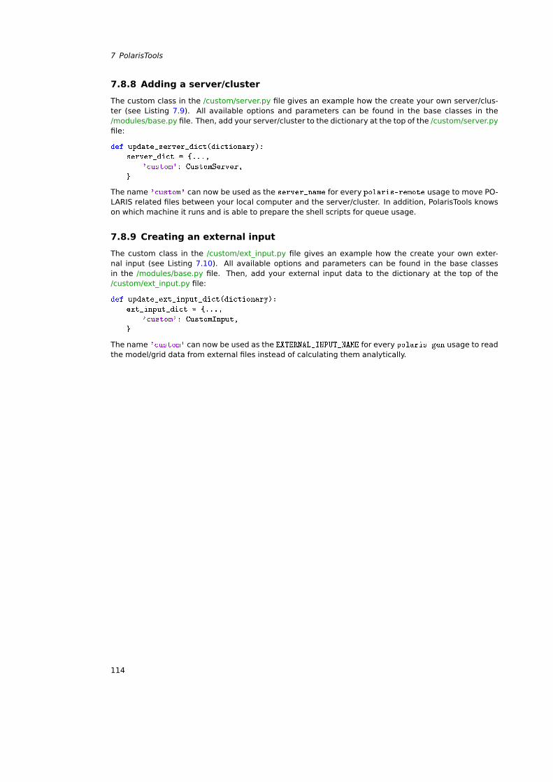
7 PolarisTools
7.8.8 Adding a server/cluster
The custom class in the /custom/server.py file gives an example how the create your own server/clus-ter (see Listing 7.9). All available options and parameters can be found in the base classes in the/modules/base.py file. Then, add your server/cluster to the dictionary at the top of the /custom/server.pyfile:
def update_server_dict(dictionary):
server_dict = ...,
'custom': CustomServer,
The name 'custom' can now be used as the server_name for every polaris-remote usage to move PO-LARIS related files between your local computer and the server/cluster. In addition, PolarisTools knowson which machine it runs and is able to prepare the shell scripts for queue usage.
7.8.9 Creating an external input
The custom class in the /custom/ext_input.py file gives an example how the create your own exter-nal input (see Listing 7.10). All available options and parameters can be found in the base classesin the /modules/base.py file. Then, add your external input data to the dictionary at the top of the/custom/ext_input.py file:
def update_ext_input_dict(dictionary):
ext_input_dict = ...,
'custom': CustomInput,
The name 'custom' can now be used as the EXTERNAL_INPUT_NAME for every polaris-gen usage to readthe model/grid data from external files instead of calculating them analytically.
114
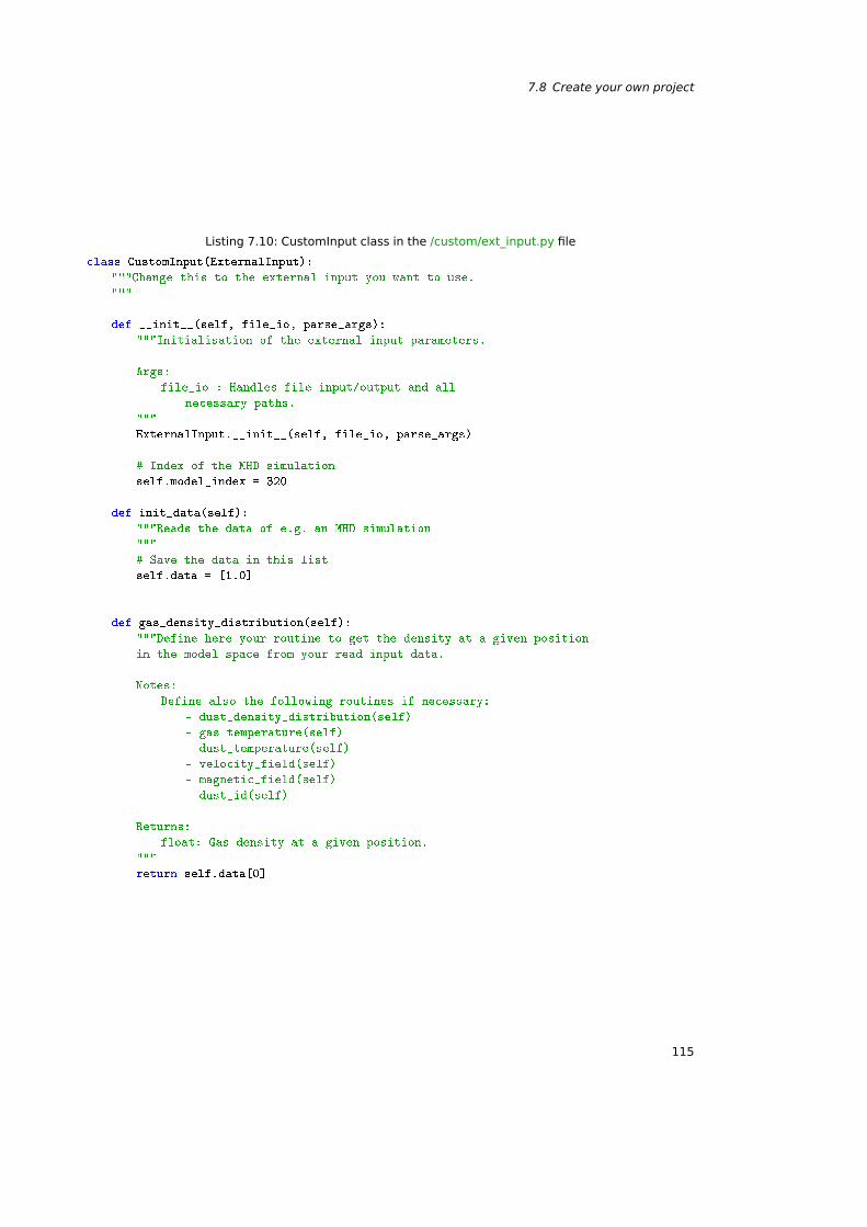
7.8 Create your own project
Listing 7.10: CustomInput class in the /custom/ext_input.py file
class CustomInput(ExternalInput):
"""Change this to the external input you want to use.
"""
def __init__(self, file_io, parse_args):
"""Initialisation of the external input parameters.
Args:
file_io : Handles file input/output and all
necessary paths.
"""
ExternalInput.__init__(self, file_io, parse_args)
# Index of the MHD simulation
self.model_index = 320
def init_data(self):
"""Reads the data of e.g. an MHD simulation
"""
# Save the data in this list
self.data = [1.0]
def gas_density_distribution(self):
"""Define here your routine to get the density at a given position
in the model space from your read input data.
Notes:
Define also the following routines if necessary:
- dust_density_distribution(self)
- gas_temperature(self)
- dust_temperature(self)
- velocity_field(self)
- magnetic_field(self)
- dust_id(self)
Returns:
float: Gas density at a given position.
"""
return self.data[0]
115
7 PolarisTools
7.9 Quickstart guide
To try out the main capabilities of POLARIS, use the following step-by-step instruction. The examplesimulations are based on a model of a circumstellar disk with characteristics shown in Table 7.19. Inthis model, we assumes compact, homogeneous, and spherical dust grains with a composition of 62.5%silicate and 37.5% graphite (MRN-dust, Mathis et al. 1977; optical properties from Weingartner & Draine2001).
We consider furthermore a density distribution with a radial decrease based on the work of Hayashi(1981) for the minimum mass solar nebular. Combined with a vertical distribution due to hydrostaticequilibrium similar to the work of Shakura & Sunyaev (1973), we obtain the following equation:
ρdisk = ρ0
(Rref
ω
)aexp
(−12
[z
H (ω)
]2). (7.1)
Here, ω is the radial distance from the central star in the disk midplane, z is the distance from themidplane of the disk, Rref is a reference radius, and H (ω) is the scale height. The density ρ0 is derivedfrom the disk (gas) mass. The scale height is a function of ω as follows:
H (ω) = h0(ω
Rref
)b. (7.2)
The parameters a and b set the radial density profile and the disk flaring, respectively.
7.9.1 Create a grid
The first step is the creation of a grid, based on the chosen model. To do this, enter the followingcommand (t ∼ 1 s):
polaris-gen disk grid.dat
Now, you have a binary file named 'grid.dat' in your projects/disk/ directory that contains a grid withcells that have physical quantities like density and temperature that are defined by the chosen model.
7.9.2 Dust temperature distribution
The dust temperature distribution can be simulated by assuming that the dust grains are in equilibriumwith the radiation field. To do this, enter the following command (t ∼ 1min):
polaris-run disk example temp --grid grid.dat --adj_tgas 1
The temperature distribution can easily be visualized by entering the following commands:
polaris-plot disk example temp midplane output dust_temperature xy
polaris-plot disk example temp midplane output dust_temperature xz
You will find the resulting PDF files in the projects/disk/example/temp/plots/ directory. The temperaturedistributions should look like those in Fig. 7.1.
7.9.3 Dust thermal emission
Based on the dust temperature distribution, the thermal emission of the dust grains at λ = 850µm canbe simulated. To do this, enter the following command (t ∼ 1min):
polaris-run disk example dust --wavelength 850e-6
The thermal emission can easily be visualized by entering the following command:
polaris-plot disk example dust map 1 --cmap_scaling power 0.5
You will find the resulting PDF file in the projects/disk/example/dust/plots/ directory. The intensity mapis scaled by the power of 0.5 and should look like Fig. 7.2.
116
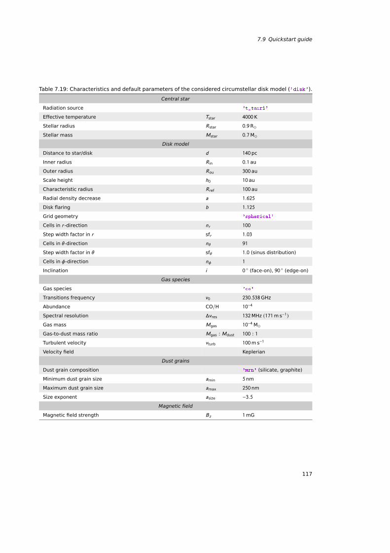
7.9 Quickstart guide
Table 7.19: Characteristics and default parameters of the considered circumstellar disk model ('disk').
Central star
Radiation source 't_tauri'
Effective temperature Tstar 4000K
Stellar radius Rstar 0.9R
Stellar mass Mstar 0.7M
Disk model
Distance to star/disk d 140pc
Inner radius R in 0.1 au
Outer radius Rou 300 au
Scale height h0 10 au
Characteristic radius Rref 100 au
Radial density decrease a 1.625
Disk flaring b 1.125
Grid geometry 'spherical'
Cells in r -direction nr 100
Step width factor in r sfr 1.03
Cells in θ-direction nθ 91
Step width factor in θ sfθ 1.0 (sinus distribution)
Cells in φ-direction nφ 1
Inclination i 0 (face-on), 90 (edge-on)
Gas species
Gas species 'co'
Transitions frequency ν0 230.538GHz
Abundance CO/H 10−4
Spectral resolution ∆νres 132MHz (171m s−1)Gas mass Mgas 10−4 M
Gas-to-dust mass ratio Mgas : Mdust 100 : 1
Turbulent velocity vturb 100m s−1
Velocity field Keplerian
Dust grains
Dust grain composition 'mrn' (silicate, graphite)
Minimum dust grain size amin 5nm
Maximum dust grain size amax 250nm
Size exponent asize −3.5Magnetic field
Magnetic field strength Bz 1mG
117
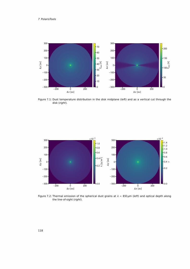
7 PolarisTools
−200 0 200∆x [au]
−300
−200
−100
0
100
200
300
∆y[au]
0
10
20
30
40
50
60
70
Tdu
st[K]
−200 0 200∆x [au]
−300
−200
−100
0
100
200
300
∆z[au]
0
50
100
150
200
Tdu
st[K]
Figure 7.1: Dust temperature distribution in the disk midplane (left) and as a vertical cut through thedisk (right).
−200 0 200∆x [au]
−300
−200
−100
0
100
200
300
∆y[au]
0.0
0.2
0.4
0.6
0.8
1.0
F I[Jy/a
s2]
×10−3
−200 0 200∆x [au]
−300
−200
−100
0
100
200
300
∆y[au]
0.0
0.2
0.4
0.6
0.8
1.0
1.21.4
τ
×10−4
Figure 7.2: Thermal emission of the spherical dust grains at λ = 850µm (left) and optical depth alongthe line-of-sight (right).
118
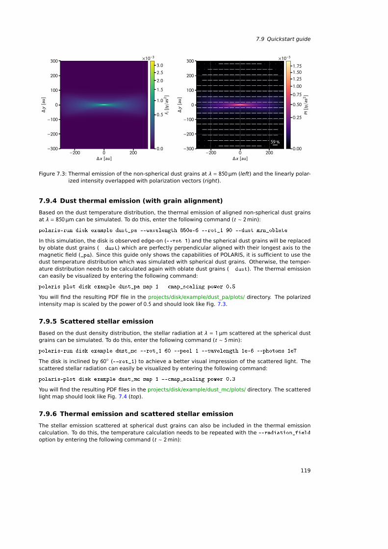
7.9 Quickstart guide
−200 0 200∆x [au]
−300
−200
−100
0
100
200
300
∆y[au]
0.0
0.5
1.0
1.5
2.0
2.5
3.0
F I[Jy/a
s2]
×10−3
59%
−200 0 200∆x [au]
−300
−200
−100
0
100
200
300
∆y[au]
0.00
0.25
0.50
0.75
1.00
1.25
1.501.75
PI[Jy/a
s2]
×10−3
Figure 7.3: Thermal emission of the non-spherical dust grains at λ = 850µm (left) and the linearly polar-ized intensity overlapped with polarization vectors (right).
7.9.4 Dust thermal emission (with grain alignment)
Based on the dust temperature distribution, the thermal emission of aligned non-spherical dust grainsat λ = 850µm can be simulated. To do this, enter the following command (t ∼ 2min):
polaris-run disk example dust_pa --wavelength 850e-6 --rot_1 90 --dust mrn_oblate
In this simulation, the disk is observed edge-on (--rot_1) and the spherical dust grains will be replacedby oblate dust grains (--dust) which are perfectly perpendicular aligned with their longest axis to themagnetic field (_pa). Since this guide only shows the capabilities of POLARIS, it is sufficient to use thedust temperature distribution which was simulated with spherical dust grains. Otherwise, the temper-ature distribution needs to be calculated again with oblate dust grains (--dust). The thermal emissioncan easily be visualized by entering the following command:
polaris-plot disk example dust_pa map 1 --cmap_scaling power 0.5
You will find the resulting PDF file in the projects/disk/example/dust_pa/plots/ directory. The polarizedintensity map is scaled by the power of 0.5 and should look like Fig. 7.3.
7.9.5 Scattered stellar emission
Based on the dust density distribution, the stellar radiation at λ = 1µm scattered at the spherical dustgrains can be simulated. To do this, enter the following command (t ∼ 5min):
polaris-run disk example dust_mc --rot_1 60 --peel 1 --wavelength 1e-6 --photons 1e7
The disk is inclined by 60 (--rot_1) to achieve a better visual impression of the scattered light. Thescattered stellar radiation can easily be visualized by entering the following command:
polaris-plot disk example dust_mc map 1 --cmap_scaling power 0.3
You will find the resulting PDF files in the projects/disk/example/dust_mc/plots/ directory. The scatteredlight map should look like Fig. 7.4 (top).
7.9.6 Thermal emission and scattered stellar emission
The stellar emission scattered at spherical dust grains can also be included in the thermal emissioncalculation. To do this, the temperature calculation needs to be repeated with the --radiation_field
option by entering the following command (t ∼ 2min):
119
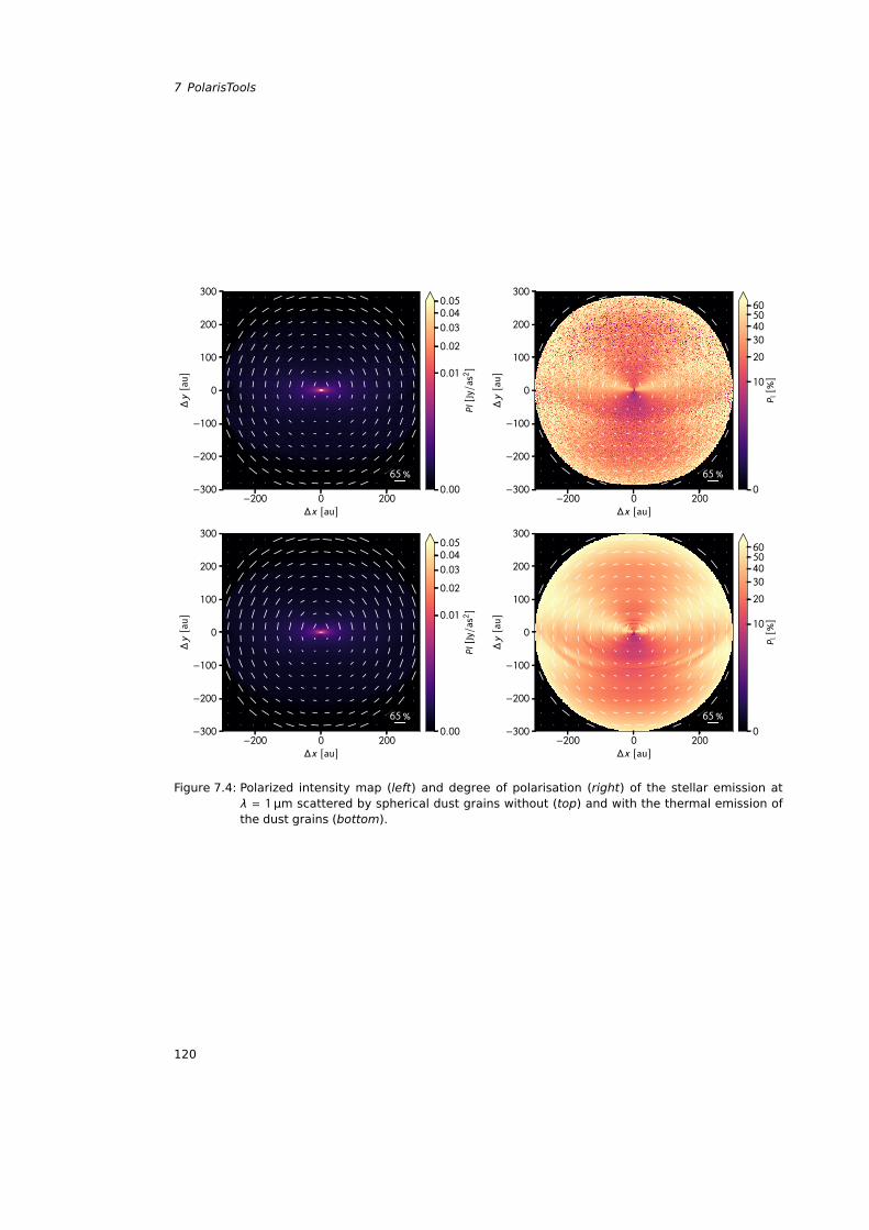
7 PolarisTools
65%
−200 0 200∆x [au]
−300
−200
−100
0
100
200
300
∆y[au]
0.00
0.01
0.02
0.03
0.040.05
PI[Jy/a
s2]
65%
−200 0 200∆x [au]
−300
−200
−100
0
100
200
300
∆y[au]
0
10
20
30405060
P l[%]
65%
−200 0 200∆x [au]
−300
−200
−100
0
100
200
300
∆y[au]
0.00
0.01
0.02
0.03
0.040.05
PI[Jy/a
s2]
65%
−200 0 200∆x [au]
−300
−200
−100
0
100
200
300
∆y[au]
0
10
20
30405060
P l[%]
Figure 7.4: Polarized intensity map (left) and degree of polarisation (right) of the stellar emission atλ = 1µm scattered by spherical dust grains without (top) and with the thermal emission ofthe dust grains (bottom).
120
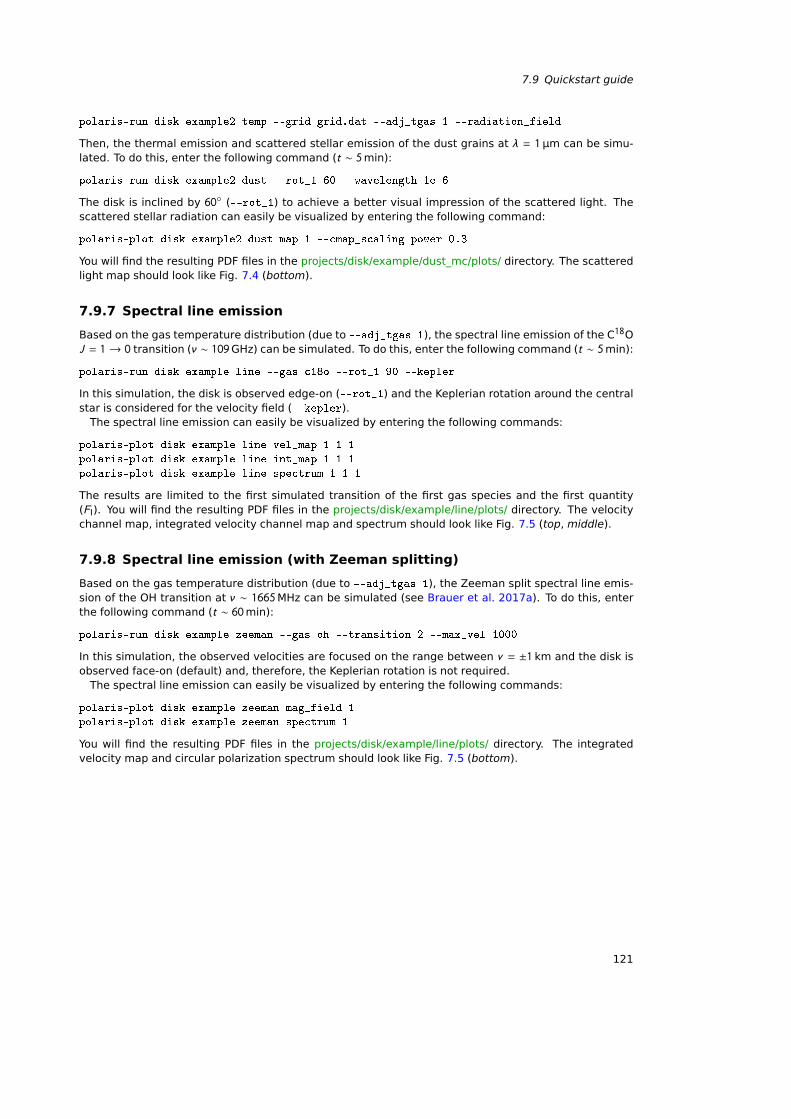
7.9 Quickstart guide
polaris-run disk example2 temp --grid grid.dat --adj_tgas 1 --radiation_field
Then, the thermal emission and scattered stellar emission of the dust grains at λ = 1µm can be simu-lated. To do this, enter the following command (t ∼ 5min):
polaris-run disk example2 dust --rot_1 60 --wavelength 1e-6
The disk is inclined by 60 (--rot_1) to achieve a better visual impression of the scattered light. Thescattered stellar radiation can easily be visualized by entering the following command:
polaris-plot disk example2 dust map 1 --cmap_scaling power 0.3
You will find the resulting PDF files in the projects/disk/example/dust_mc/plots/ directory. The scatteredlight map should look like Fig. 7.4 (bottom).
7.9.7 Spectral line emission
Based on the gas temperature distribution (due to --adj_tgas 1), the spectral line emission of the C18OJ = 1→ 0 transition (ν ∼ 109GHz) can be simulated. To do this, enter the following command (t ∼ 5min):
polaris-run disk example line --gas c18o --rot_1 90 --kepler
In this simulation, the disk is observed edge-on (--rot_1) and the Keplerian rotation around the centralstar is considered for the velocity field (--kepler).
The spectral line emission can easily be visualized by entering the following commands:
polaris-plot disk example line vel_map 1 1 1
polaris-plot disk example line int_map 1 1 1
polaris-plot disk example line spectrum 1 1 1
The results are limited to the first simulated transition of the first gas species and the first quantity(FI). You will find the resulting PDF files in the projects/disk/example/line/plots/ directory. The velocitychannel map, integrated velocity channel map and spectrum should look like Fig. 7.5 (top, middle).
7.9.8 Spectral line emission (with Zeeman splitting)
Based on the gas temperature distribution (due to --adj_tgas 1), the Zeeman split spectral line emis-sion of the OH transition at ν ∼ 1665MHz can be simulated (see Brauer et al. 2017a). To do this, enterthe following command (t ∼ 60min):
polaris-run disk example zeeman --gas oh --transition 2 --max_vel 1000
In this simulation, the observed velocities are focused on the range between v = ±1 km and the disk isobserved face-on (default) and, therefore, the Keplerian rotation is not required.
The spectral line emission can easily be visualized by entering the following commands:
polaris-plot disk example zeeman mag_field 1
polaris-plot disk example zeeman spectrum 1
You will find the resulting PDF files in the projects/disk/example/line/plots/ directory. The integratedvelocity map and circular polarization spectrum should look like Fig. 7.5 (bottom).
121
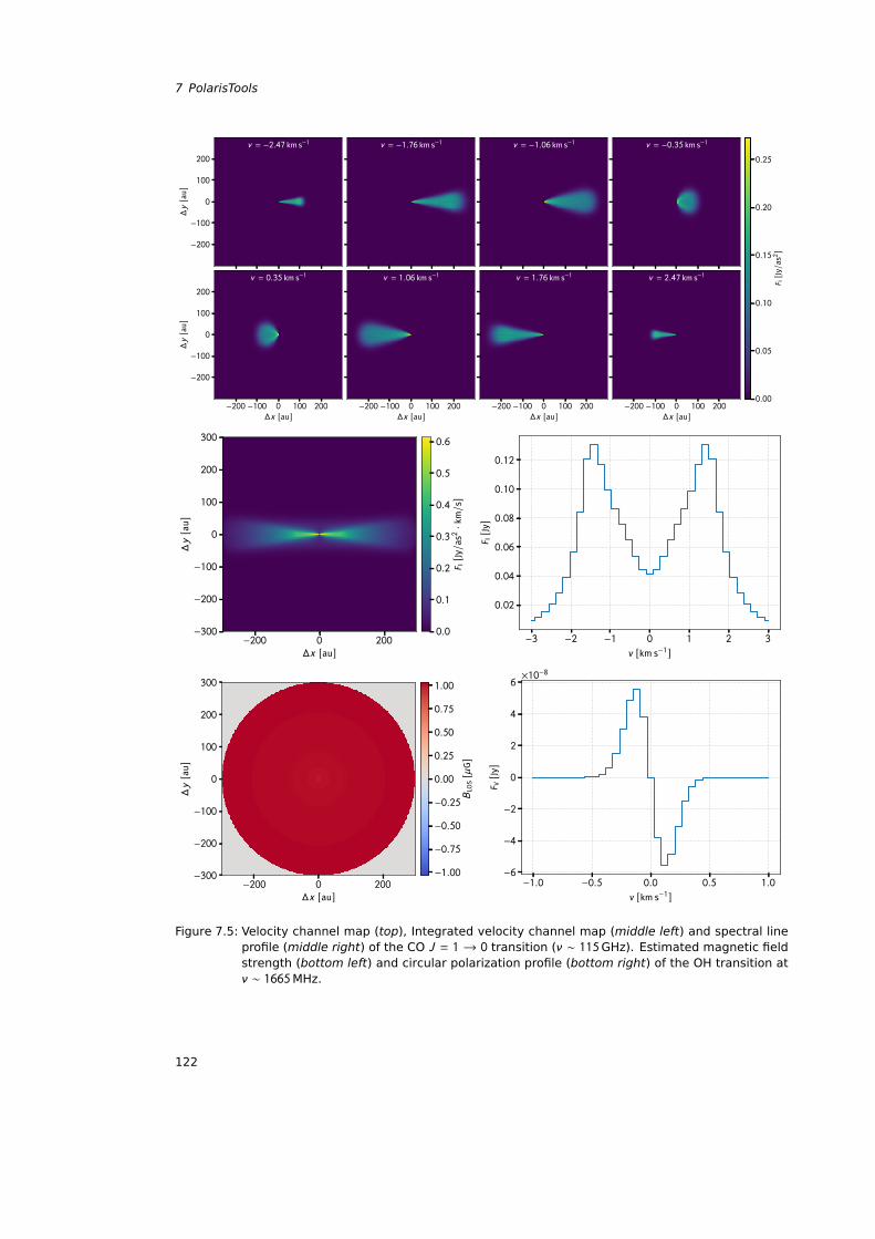
7 PolarisTools
−200
−100
0
100
200
∆y[au]
v = −2.47 km s−1 v = −1.76 km s−1 v = −1.06 km s−1 v = −0.35 km s−1
−200 −100 0 100 200∆x [au]
−200
−100
0
100
200
∆y[au]
v = 0.35 km s−1
−200 −100 0 100 200∆x [au]
v = 1.06 km s−1
−200 −100 0 100 200∆x [au]
v = 1.76 km s−1
−200 −100 0 100 200∆x [au]
v = 2.47 km s−1
0.00
0.05
0.10
0.15
0.20
0.25
F I[Jy/a
s2]
−200 0 200∆x [au]
−300
−200
−100
0
100
200
300
∆y[au]
0.0
0.1
0.2
0.3
0.4
0.5
0.6
F I[Jy/a
s2·k
m/s]
−3 −2 −1 0 1 2 3
v [km s−1]
0.02
0.04
0.06
0.08
0.10
0.12
F I[Jy]
−200 0 200∆x [au]
−300
−200
−100
0
100
200
300
∆y[au]
−1.00
−0.75
−0.50
−0.25
0.00
0.25
0.50
0.75
1.00
BLO
S[µ
G]
−1.0 −0.5 0.0 0.5 1.0
v [km s−1]
−6
−4
−2
0
2
4
6
F V[Jy]
×10−8
Figure 7.5: Velocity channel map (top), Integrated velocity channel map (middle left) and spectral lineprofile (middle right) of the CO J = 1 → 0 transition (ν ∼ 115GHz). Estimated magnetic fieldstrength (bottom left) and circular polarization profile (bottom right) of the OH transition atν ∼ 1665MHz.
122
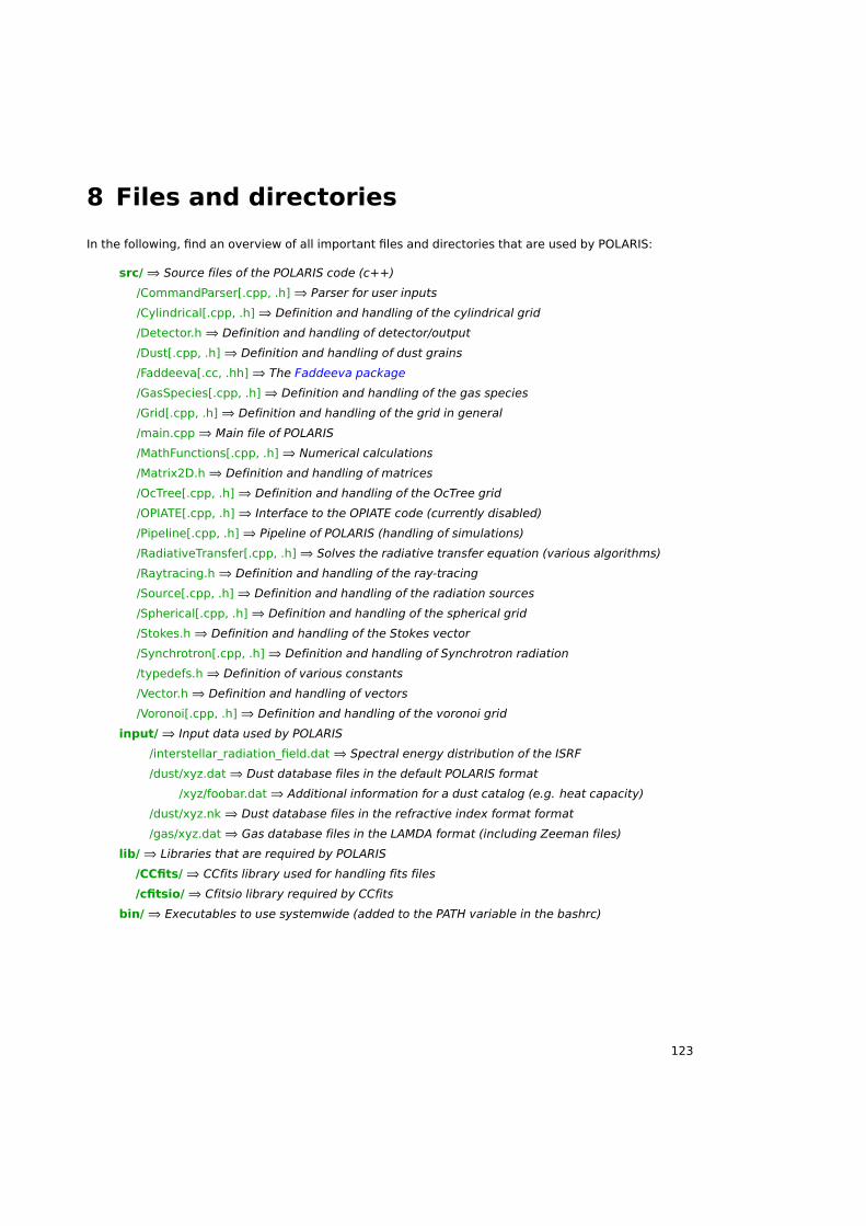
8 Files and directories
In the following, find an overview of all important files and directories that are used by POLARIS:
src/⇒ Source files of the POLARIS code (c++)
/CommandParser[.cpp, .h]⇒ Parser for user inputs
/Cylindrical[.cpp, .h]⇒ Definition and handling of the cylindrical grid
/Detector.h⇒ Definition and handling of detector/output
/Dust[.cpp, .h]⇒ Definition and handling of dust grains
/Faddeeva[.cc, .hh]⇒ The Faddeeva package
/GasSpecies[.cpp, .h]⇒ Definition and handling of the gas species
/Grid[.cpp, .h]⇒ Definition and handling of the grid in general
/main.cpp⇒ Main file of POLARIS
/MathFunctions[.cpp, .h]⇒ Numerical calculations
/Matrix2D.h⇒ Definition and handling of matrices
/OcTree[.cpp, .h]⇒ Definition and handling of the OcTree grid
/OPIATE[.cpp, .h]⇒ Interface to the OPIATE code (currently disabled)
/Pipeline[.cpp, .h]⇒ Pipeline of POLARIS (handling of simulations)
/RadiativeTransfer[.cpp, .h]⇒ Solves the radiative transfer equation (various algorithms)
/Raytracing.h⇒ Definition and handling of the ray-tracing
/Source[.cpp, .h]⇒ Definition and handling of the radiation sources
/Spherical[.cpp, .h]⇒ Definition and handling of the spherical grid
/Stokes.h⇒ Definition and handling of the Stokes vector
/Synchrotron[.cpp, .h]⇒ Definition and handling of Synchrotron radiation
/typedefs.h⇒ Definition of various constants
/Vector.h⇒ Definition and handling of vectors
/Voronoi[.cpp, .h]⇒ Definition and handling of the voronoi grid
input/⇒ Input data used by POLARIS
/interstellar_radiation_field.dat⇒ Spectral energy distribution of the ISRF
/dust/xyz.dat⇒ Dust database files in the default POLARIS format
/xyz/foobar.dat⇒ Additional information for a dust catalog (e.g. heat capacity)
/dust/xyz.nk⇒ Dust database files in the refractive index format format
/gas/xyz.dat⇒ Gas database files in the LAMDA format (including Zeeman files)
lib/⇒ Libraries that are required by POLARIS
/CCfits/⇒ CCfits library used for handling fits files
/cfitsio/⇒ Cfitsio library required by CCfits
bin/⇒ Executables to use systemwide (added to the PATH variable in the bashrc)
123
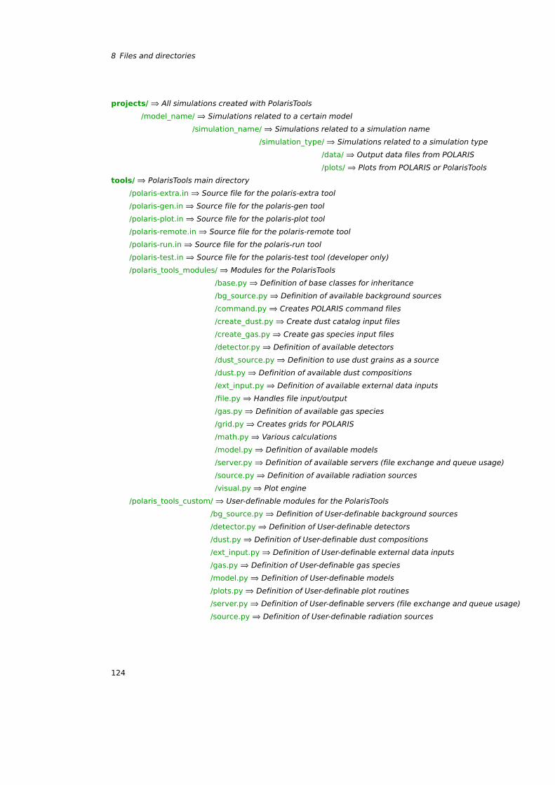
8 Files and directories
projects/⇒ All simulations created with PolarisTools
/model_name/⇒ Simulations related to a certain model
/simulation_name/⇒ Simulations related to a simulation name
/simulation_type/⇒ Simulations related to a simulation type
/data/⇒ Output data files from POLARIS
/plots/⇒ Plots from POLARIS or PolarisTools
tools/⇒ PolarisTools main directory
/polaris-extra.in⇒ Source file for the polaris-extra tool
/polaris-gen.in⇒ Source file for the polaris-gen tool
/polaris-plot.in⇒ Source file for the polaris-plot tool
/polaris-remote.in⇒ Source file for the polaris-remote tool
/polaris-run.in⇒ Source file for the polaris-run tool
/polaris-test.in⇒ Source file for the polaris-test tool (developer only)
/polaris_tools_modules/⇒ Modules for the PolarisTools
/base.py⇒ Definition of base classes for inheritance
/bg_source.py⇒ Definition of available background sources
/command.py⇒ Creates POLARIS command files
/create_dust.py⇒ Create dust catalog input files
/create_gas.py⇒ Create gas species input files
/detector.py⇒ Definition of available detectors
/dust_source.py⇒ Definition to use dust grains as a source
/dust.py⇒ Definition of available dust compositions
/ext_input.py⇒ Definition of available external data inputs
/file.py⇒ Handles file input/output
/gas.py⇒ Definition of available gas species
/grid.py⇒ Creates grids for POLARIS
/math.py⇒ Various calculations
/model.py⇒ Definition of available models
/server.py⇒ Definition of available servers (file exchange and queue usage)
/source.py⇒ Definition of available radiation sources
/visual.py⇒ Plot engine
/polaris_tools_custom/⇒ User-definable modules for the PolarisTools
/bg_source.py⇒ Definition of User-definable background sources
/detector.py⇒ Definition of User-definable detectors
/dust.py⇒ Definition of User-definable dust compositions
/ext_input.py⇒ Definition of User-definable external data inputs
/gas.py⇒ Definition of User-definable gas species
/model.py⇒ Definition of User-definable models
/plots.py⇒ Definition of User-definable plot routines
/server.py⇒ Definition of User-definable servers (file exchange and queue usage)
/source.py⇒ Definition of User-definable radiation sources
124
9 Changelog
The following list provides an overview of the fixed bugs and changes made in the last updates ofPOLARIS.
Version 4.05 ⇒ 4.06
• Moved from autotools to cmake building tools (more flexible)
– Please use ./install_polaris.sh to update your installation of POLARIS (let us know ifyou have any problems)
– By moving to cmake, we should be better suited to support MacOS (fully) and Windows
– Added installer option ’-c’ to allow pre-compiled POLARIS binaries
• PolarisTools will now be installed locally as a normal python package
– Changed the directories of PolarisTools (see Chapter 8)
• Updated radiation field approach for self-scattering
• Fixing various problems of PolarisTools and adding support for laser source
Version 4.04 ⇒ 4.05
• Speed up of several routines and simulation modes
• Added slice raytracing detector to synchrotron simulations
• Added Laser radiation source to available sources (see 4.2)
• Added the option to modify the dust size distribution in each cell by defining an exponential slopeq in each grid cell (see 3.3)
• Fixed problem with some gas catalog files and their collisional data
• Fixed installation issues with existing python installations
• Fixed acceptance angle for simulations without peel-off technique. The unit is now degrees as itused to be.
Version 4.03 ⇒ 4.04
• The size of the sphere for the ISRF can now be defined (see Sect. 4.2)
• The gas-to-dust mass ratio can be set individually as the dust mass fractions, if the globalmass_fraction is set to zero (see Sect. 3.1)
• Optimized code to prevent a bottleneck when the treatment of a single photon package is veryfast
• The dust choice IDs in the grid can now be arbitrary and do not have to start with 0 (as it wasintended).
125
9 Changelog
• Fixed a bug when using multiple line detectors
• Fixed a bug when simulating aligned dust grains with significant extinction (e.g. short wave-lengths)
Version 4.02 ⇒ 4.03
• Added option to use the Mathis ISRF without SED file (see Sect. 4.2)
• Updated the use of the refractive index and Mie scattering calculation to the Wolf & Voshchinnikovapproach (see Sect. 3.4.3).
• In addition to the grain alignment radius aalg, the output midplane files of RAT simulations containnow also the average radiation field anisotropy and the average cosine between radiation fieldand magnetic field.
• In addition to other quantities, the output midplane files of TEMP and/or RAT simulations and theinput midplane files of simulations that use the radiation field may include now also the radiationfield and the Mathis field G0 value (see Table 3.8).
• The RAT alignment considers now also the influence of IR photons on the grain alignment.
• Fixed a wrong mixing of dust components to a dust mixture if the components have different sizedistributions (limits and shape) and bulk densities.
Version 4.01 ⇒ 4.02
• Cylindrical and spherical grids need now a value for the distribution of the ϕ-cells (fϕ) and havegenerally more options (see Sects. 3.3.2 and 3.3.3). The PolarisTools offer an option to updateolder grids (see Table 7.2).
• Optical properties for spherical dust grains can now be calculated from files containing the re-fractive index (see Sect. 3.4.3). Some of the shipped dust catalogs were updated accordingly(change for instance 'silicate.dat' ⇒ 'silicate.nk' in the command files). Even when notshipped anymore, the '.dat' catalogs of the spherical dust grains are still working with POLARIS.
• Stochastic heating can be calculated with CMD_TEMP and CMD_TEMP_RAT simulations by simplydefining the stochastic heating grain size limit (see Sect 4.6.2). The grid will contain an effectivedust temperature for each grain lower than the stochastic heating size limit. This is only anapproximation and will be less accurate than the usage of the radiation field, but will requiremuch less hard drive space.
• Even without a saved radiation field, the scattered light can be considered in raytracing simula-tions, if any star and/or the dust source is defined (see Sect. 4.6.5). These sources will be usedto calculate the radiation field before calculating the raytracing result.
• Added the <path_grid_cgs> option to set the conversion factor automatically for input grids incgs (see Sect. 3.3.6).
• Fixed a unit problem with aligned radii calculation for RATs (affecting CMD_RAT and CMD_TEMP_RAT)
• Fixed several display errors.
• Updated behavior of the polar RT grid.
• Fixed problems with mixing dust components with different grain size distributions.
• Fixed the emission/extinction of multiple dust/density distributions.
126
• Fixed adding direct emission of stars on healpix raytracing maps.
• Removed adding star direct emission of stars on slice raytracing maps.
• Fixed shift of raytracing detector to allow negative values.
• Updated hints for critical behavior.
• The scattering matrix elements S11 and S22 are saved as a gnuplot file in addition to the otherdust plots (if the scattering matrix is available).
Version 4.00 ⇒ 4.01
• Improved SED calculation for polar raytracing grid.
• Fixed a bug that not correctly mixed multiple density distributions.
• Improved the stability of the Raytracer.
127

Index
<adj_tgas>, 44<align>, 43<axis1>, 38<axis2>, 38<common>, 7<conv_dens>, 7, 18<conv_len>, 18<conv_mag>, 18<conv_vel>, 18<delta0>, 46<detector_dust nr_pixel = ">, 39, 40<detector_dust_healpix nr_sides = ">, 40, 41<detector_dust_mc nr_bins = ">, 54<detector_dust_mc nr_pixel = ">, 38<detector_line nr_pixel = ">, 39<detector_line_healpix nr_sides = ">, 40<dust_component>, 7, 51<dust_offset>, 43, 44<enfsca>, 7, 36, 53<f_c>, 43, 52<f_highJ>, 47, 52<gas_species vel_channels = "">, 56<larm_f>, 47<mass_fraction>, 7, 18<max_lines>, 7<max_subpixel_lvl>, 36<mu>, 18, 47<nr_gnu_points>, 7<nr_gnu_vectors>, 7<nr_threads>, 7<path_grid>, 7<path_out>, 7<phase_function>, 41, 53<plot_out_midplanes>, 7<source_background nr_photons = "">, 34<source_dust nr_photons = "">, 35<source_dust nr_photons = "">, 34<source_isrf nr_photons = "">, 7, 34<source_laser nr_photons = "">, 35<source_laser nr_photons = "">, 35<source_star nr_photons = "">, 7, 32<source_starfield nr_photons = "">, 33<task>, 7<write_out_midplanes>, 7
abundance, 11
albedo, 31, 32ALIG_GOLD, 46, 48ALIG_IDG, 46, 48ALIG_INTERNAL, 45, 48, 52ALIG_RAT, 47, 48alignment, angle, 43alignment, anisotropy factor, energy density, 47,
48alignment, anisotropy factor, gas stream, 46alignment, correlation factor, 43alignment, Gold, magneto mechanical, 46alignment, Imperfect Davis – Greenstein (IDG),
46alignment, imperfect internal, 45alignment, Larmor limit, 47alignment, Mach limit, 47alignment, omega ratio, 47alignment, Radiative torque (RAT), 47alignment, Rayleigh reduction factor, 43alignment, theories, 43AMIRA, 77anisotropic scattering, 41anisotropy factor, 11argument, 7attractor point, 47
Bohr magneton, 57Boltzmann distribution, 45, 56
CMD_DUST_EMISSION, 51CMD_DUST_SCATTERING, 53CMD_RAT, 48CMD_TEMP, 7collision rate, 55column density, 30command file, 7command file,old commands, new commands,
changed commands, 9comments, 7common, 7correlation factor, 43cross sections matrix, 48cylindrical grid, 14
Davis - Greenstein, 46Davis - Greenstein effect, 46
129
Index
DDSCAT, 18degeneracy, 57degree of circular polarization, 29degree of linear polarization, 29detector, 38detector, plane, 38detector, spherical, 38Doppler broadening, 60dust grain alignment radius, 11, 47, 48dust mass density, 11dust number density, 11dust temperature, 11, 42dust, alignment theories, 43dust, cross section file, 18dust, description string, 19dust, minimal grain radius, 11dust, parameters file, 18dust, radius, 19dust, refractive index file, 20dust, scattering matrix file, 19dust, size exponent, 11
Einstein coefficient, 55energy density, 47, 48energy level, 55enforced first scattering, 36
Fadeeva, function, 60Fadeeva, package, 61full escape probability (FEP), 56
gas mass density, 11gas number density, 11gas species, abundance, 11, 57gas species, database, 21gas species, excitation, 56gas species, name, 22gas species, parameters file, 21gas species, polarization rotation matrices, 60gas species, radius, 22gas species, ratio, 11gas temperature, 11, 42gas velocity, 11gas, kinetic temperature, 56Gaussian elimination, 56Gnuplot, 73gnuplot, 7Gold, 46grain alignment theories, 43grid header, 9grid physical parameters ID, 11grid type ID, 10grid types, 9grid, cylindrical, 14grid, octree, 15
grid, output, 67grid, rotation, 38grid, spherical, 10grid, voronoi, 17grid_rat.dat, 48
HEALPIX, 40Heisenberg’s uncertainty principle, 60Henyey-Greenstein, 19, 41
input files, 7interstellar radiation field (ISRF), 7, 34isotropic scattering, 41ISRF, 34
LAMDA, 21Landè factor, 22, 61large velocity gradient (LVG), 57Larmor limit, 47level populations, 56line of sight magnetic field strength, 61line radiative transfer, 21, 55line strength, 59, 60Linux, 67Local thermodynamic equilibrium (LTE), 32, 42local thermodynamic equilibrium (LTE), 56
Mach number, 47magnetic field, 11magnetic quantum number, 57magneto-optical effects, 59maximal dust grain radius, 11Mie scattering, 42MIEX, 18minimal dust grain radius, 11modified black body spectrum, 32Müller matrix, 19, 51
noise, 32noise estimation, 32
octree grid, 15optical depth, 30, 31, 36, 37, 57optical depth, statistical function, 31optimization techniques, 36optimization, enforced first scattering, 36optimization, peel-off technique, 37optimization, wavelength range selection, 38
peel-off technique, 37PH_HG, 41PH_ISO, 41PH_MIE, 42, 53phase function, Henyey-Greenstein (HG), 19, 41phase functions, 41photon emitting sources, 32
130
Index
photon package, 29photon, MC transfer, 31photon, propagation, 29plane detector, 38polarization by non-spherical dust grains, 48polarization, scattering, 51POP_FEP, 61POP_LTE, 56POP_LVG, 57position angle, 29pressure broadening, 60
quantum numbers, 57
radiation field, 11radiative pressure, 11ray-tracing, 32Rayleigh reduction factor, combination of, 48Rayleigh reduction factor, combined, 48Rayleigh reduction factor, definition, 43rotation, axis, 34, 38rotation, grid, 38Runge-Kutta Fehlberg, 30
scattering matrix, 19, 51scattering, anisotropic, 41scattering, Henyey-Greenstein, 42scattering, isotropic, 41scattering, Mie, 42scattering, phase function, 53scattering, relevance of, 32scattering, rotation, 53shape parameter, 10size exponent, 11skip cell in RT, 10source, 35source, dust, 34source, ISRF, 34source, star, 32source, starfield, 33sources, 32spectral energy distribution (SED), 7, 33, 38spherical detector, 38spherical grid, 10star, 32starfield, 33step size, 30, 31step size, maximal number of, 31step size, Runge-Kutta, 30, 31Stokes I, 29Stokes Q, 29Stokes U, 29Stokes V, 29Stokes vector, 29sub-level, 57
sub-pixel level, 36sub-pixeling, 36synchrotron, 61
task, 7temperature, dust, 11temperature, gas, 11temperature, sampling function, 32, 42temperatures, range, 42transition, 57turbulent velocity, 11typedefs.h, 31, 33, 36
unit, cgs, 9, 18unit, conversion, 18unit, SI, 9, 18, 67
velocity bins, 39velocity gradient, 57velocity range, 39velocity, gas, 11velocity, maximal observable, 39voronoi grid, 17
wavelength range selection, 38Windows, 67
Zeeman, parameters file, 22
131

Bibliography
Bjorkman, J. E. & Wood, K. 2001, The Astrophysical Journal, 554, 615
Bohren, C. F. & Huffman, D. R. 1983, Absorption and scattering of light by small particles
Brauer, R., Wolf, S., & Flock, M. 2017a, Astronomy and Astrophysics, 607, A104
Brauer, R., Wolf, S., & Reissl, S. 2016, Astronomy & Astrophysics, 588, A129
Brauer, R., Wolf, S., Reissl, S., & Ober, F. 2017b, Astronomy & Astrophysics, 601, A90
Camps, P., Misselt, K., Bianchi, S., et al. 2015, Astronomy & Astrophysics, 580, A87
Cashwell, E. D. 1957, A practical manual on the Monte Carlo method for random walk problems / (LosAlamos, N.M. :)
Davis, Jr., L. & Greenstein, J. L. 1951, The Astrophysical Journal, 114, 206
Dexter, J. 2016, Monthly Notices of the Royal Astronomical Society, 462, 115
Draine, B. T. & Flatau, P. J. 2013, ArXiv e-prints, 1305, arXiv:1305.6497
Draine, B. T. & Weingartner, J. C. 1996, \apj, 470, 551, arXiv: astro-ph/9605046
Draine, B. T. & Weingartner, J. C. 1997, The Astrophysical Journal, 480, 633
Evans, II, N. J., Rawlings, J. M. C., Shirley, Y. L., & Mundy, L. G. 2001, The Astrophysical Journal, 557, 193
Gold, T. 1952, Monthly Notices of the Royal Astronomical Society, 112, 215
Gordon, K. D., Misselt, K. A., Witt, A. N., & Clayton, G. C. 2001, The Astrophysical Journal, 551, 269
Hayashi, C. 1981, Progress of Theoretical Physics Supplement, 70, 35
Hoang, T., Nguyen-Quynh, L., Nguyen-Anh, V., & Kim, Y.-J. 2018, ArXiv e-prints
Jones, A. P., Fanciullo, L., Koehler, M., et al. 2014, published; A&A 558, A62 (2013), 558, A62, arXiv:1411.6293v1
Jones, A. P., Koehler, M., Ysard, N., Bocchio, M., & Verstraete, L. 2017, A&A 602, A46 (2017), 602, A46,arXiv: 1703.00775v1
Larsson, R., Buehler, S. A., Eriksson, P., & Mendrok, J. 2014, Journal of Quantitative Spectroscopy andRadiative Transfer, 133, 445
Lazarian, A. 1995, The Astrophysical Journal, 451, 660
Lazarian, A. & Efroimsky, M. 1996, The Astrophysical Journal, 466, 274
Lazarian, A., Efroimsky, M., & Ozik, J. 1996, The Astrophysical Journal, 472, 240
Lazarian, A. & Hoang, T. 2007, Monthly Notices of the Royal Astronomical Society, 378, 910
Lazarian, A. & Roberge, W. G. 1997, The Astrophysical Journal, 484, 230
Lucy, L. B. 1999, Astronomy and Astrophysics, 344, 282
Mathis, J. S., Mezger, P. G., & Panagia, N. 1983, Astronomy and Astrophysics, 128, 212
133
Bibliography
Mathis, J. S., Rumpl, W., & Nordsieck, K. H. 1977, The Astrophysical Journal, 217, 425
Ober, F., Wolf, S., Uribe, A. L., & Klahr, H. H. 2015, Astronomy & Astrophysics, 579, A105
Pandya, A., Zhang, Z., Chandra, M., & Gammie, C. F. 2016, The Astrophysical Journal, 822, 34
Reissl, S., Seifried, D., Wolf, S., Banerjee, R., & Klessen, R. S. 2017, Astronomy & Astrophysics, 603, A71
Reissl, S., Stutz, A. M., Brauer, R., et al. 2018, Monthly Notices of the Royal Astronomical Society, 481,2507
Reissl, S., Wolf, S., & Brauer, R. 2016, Astronomy and Astrophysics, 593, A87, arXiv: 1604.05305
Reissl, S., Wolf, S., & Seifried, D. 2014, Astronomy and Astrophysics, 566, A65
Seifried, D., Walch, S., Reissl, S., & Ibáñez-Mejía, J. C. 2019, Mon Not R Astron Soc, 482, 2697
Shakura, N. I. & Sunyaev, R. A. 1973, Astronomy & Astrophysics, 24
Spitzer, L. & McGlynn, T. A. 1979, The Astrophysical Journal, 231, 417
Weingartner, J. C. & Draine, B. T. 2001, The Astrophysical Journal, 548, 296
Weingartner, J. C. & Draine, B. T. 2003, The Astrophysical Journal, 589, 289
Wolf, S. 2003, Computer Physics Communications, 150, 99
Wolf, S. 2006, Astrophysics Software Database, 6
Wolf, S., Henning, T., & Stecklum, B. 1999, Astronomy and Astrophysics, 349, 839
Wolf, S. & Voshchinnikov, N. V. 2004, Computer Physics Communications, 162, 113
Yusef-Zadeh, F., Morris, M., & White, R. L. 1984, The Astrophysical Journal, 278, 186
Zhu, Z. & Stone, J. M. 2014, The Astrophysical Journal, 795, 53
134


![Technical Bulletin - Polaris - Polaris 9300 Sport & Polaris 9300xi Sport[1]](https://img.pdfslide.us/doc/110x75/553b235d4a7959d8258b463f/technical-bulletin-polaris-polaris-9300-sport-polaris-9300xi-sport1.jpg)