Pointed Hopf Algebraslibrary.msri.org/books/Book43/files/andrus.pdfpointed Hopf algebras A with abelian group of group-likes G(A) and in-ﬁnitesimal braiding of type An (up to some

New Directions in Hopf AlgebrasMSRI PublicationsVolume 43, 2002

Pointed Hopf Algebras

NICOLAS ANDRUSKIEWITSCH AND HANS-JURGEN SCHNEIDER

Abstract. This is a survey on pointed Hopf algebras over algebraicallyclosed fields of characteristic 0. We propose to classify pointed Hopf al-gebras A by first determining the graded Hopf algebra grA associated tothe coradical filtration of A. The A0-coinvariants elements form a braidedHopf algebra R in the category of Yetter–Drinfeld modules over the corad-ical A0 = |Γ, Γ the group of group-like elements of A, and gr A ' R#A0.We call the braiding of the primitive elements of R the infinitesimal braid-ing of A. If this braiding is of Cartan type [AS2], then it is often possibleto determine R, to show that R is generated as an algebra by its prim-itive elements and finally to compute all deformations or liftings, that ispointed Hopf algebras such that gr A ' R#|Γ. In the last chapter, as a con-crete illustration of the method, we describe explicitly all finite-dimensionalpointed Hopf algebras A with abelian group of group-likes G(A) and in-finitesimal braiding of type An (up to some exceptional cases). In otherwords, we compute all the liftings of type An; this result is our main newcontribution in this paper.

Contents

Introduction 21. Braided Hopf Algebras 52. Nichols Algebras 163. Types of Nichols Algebras 244. Nichols Algebras of Cartan Type 345. Classification of Pointed Hopf Algebras by the Lifting Method 376. Pointed Hopf Algebras of Type An 46References 65

2000 Mathematics Subject Classification. Primary: 17B37; Secondary: 16W30.

Key words and phrases. Pointed Hopf algebras, finite quantum groups.

This work was partially supported by ANPCyT, Agencia Cordoba Ciencia, CONICET, DAAD,the Graduiertenkolleg of the Math. Institut (Universitat Munchen) and Secyt (UNC).

1

2 NICOLAS ANDRUSKIEWITSCH AND HANS-JURGEN SCHNEIDER

Introduction

A Hopf algebra A over a field k is called pointed [Sw], [M1], if all its simpleleft or right comodules are one-dimensional. The coradical A0 of A is the sumof all its simple subcoalgebras. Thus A is pointed if and only if A0 is a groupalgebra.

We will always assume that the field k is algebraically closed of characteristic0 (although several results of the paper hold over arbitrary fields).

It is easy to see that A is pointed if it is generated as an algebra by group-likeand skew-primitive elements. In particular, group algebras, universal envelop-ing algebras of Lie algebras and the q-deformations of the universal envelopingalgebras of semisimple Lie algebras are all pointed.

An essential tool in the study of pointed Hopf algebras is the coradical filtration

A0 ⊂ A1 ⊂ · · · ⊂ A,⋃

n≥0

An = A

of A. It is dual to the filtration of an algebra by the powers of the Jacobson rad-ical. For pointed Hopf algebras it is a Hopf algebra filtration, and the associatedgraded Hopf algebra gr A has a Hopf algebra projection onto A0 = kΓ, Γ = G(A)the group of all group-like elements of A. By a theorem of Radford [Ra], gr A isa biproduct

gr A ∼= R#kΓ,

where R is a graded braided Hopf algebra in the category of left Yetter–Drinfeldmodules over kΓ [AS2].

This decomposition is an analog of the theorem of Cartier–Kostant–Milnor–Moore on the semidirect product decomposition of a cocommutative Hopf algebrainto an infinitesimal and a group algebra part.

The vector space V = P (R) of the primitive elements of R is a Yetter–Drinfeldsubmodule. We call its braiding

c : V ⊗ V → V ⊗ V

the infinitesimal braiding of A. The infinitesimal braiding is the key to thestructure of pointed Hopf algebras.

The subalgebra B(V ) of R generated by V is a braided Hopf subalgebra. Asan algebra and coalgebra, B(V ) only depends on the infinitesimal braiding ofV . In his thesis [N] published in 1978, Nichols studied Hopf algebras of theform B(V )#kΓ under the name of bialgebras of type one. We call B(V ) theNichols algebra of V . These Hopf algebras were found independently later byWoronowicz [Wo] and other authors.

Important examples of Nichols algebras come from quantum groups [Dr1].If g is a semisimple Lie algebra, U≥0

q (g), q not a root of unity, and the finite-dimensional Frobenius–Lusztig kernels u≥0

q (g), q a root of unity of order N , are

POINTED HOPF ALGEBRAS 3

both of the form B(V )#kΓ with Γ = Zθ resp. (Z/(N))θ, θ ≥ 1. ([L3], [Ro1],[Sbg], and [L2], [Ro1], [Mu]) (assuming some technical conditions on N).

In general, the classification problem of pointed Hopf algebras has three parts:

(1) Structure of the Nichols algebras B(V ).(2) The lifting problem: Determine the structure of all pointed Hopf algebras A

with G(A) = Γ such that gr A ∼= B(V )#kΓ.(3) Generation in degree one: Decide which Hopf algebras A are generated by

group-like and skew-primitive elements, that is gr A is generated in degreeone.

We conjecture that all finite-dimensional pointed Hopf algebras over an alge-braically closed field of characteristic 0 are indeed generated by group-like andskew-primitive elements.

In this paper, we describe the steps of this program in detail and explain thepositive results obtained so far in this direction. It is not our intention to give acomplete survey on all aspects of pointed Hopf algebras.

We will mainly report on recent progress in the classification of pointed Hopfalgebras with abelian group of group-like elements.

If the group Γ is abelian, and V is a finite-dimensional Yetter–Drinfeld module,then the braiding is given by a family of non-zero scalars qij ∈ k, 1 ≤ i ≤ θ, inthe form

c(xi ⊗ xj) = qijxj ⊗ xi, where x1, . . . , xθ is a basis of V.

Moreover there are elements g1, . . . , gθ ∈ Γ, and characters χ1, . . . , χθ ∈ Γ suchthat qij = χj(gi). The group acts on xi via the character χi, and xi is a gi-homogeneous element with respect to the coaction of Γ. We introduced braidingsof Cartan type [AS2] where

qijqji = qaij

ii , 1 ≤ i, j ≤ θ, and (aij) is a generalized Cartan matrix.

If (aij) is a Cartan matrix of finite type, then the algebras B(V ) can be under-stood as twisting of the Frobenius–Lusztig kernels u≥0(g), g a semisimple Liealgebra.

By deforming the quantum Serre relations for simple roots which lie in two dif-ferent connected components of the Dynkin diagram, we define finite-dimensionalpointed Hopf algebras u(D) in terms of a ”linking datum D of finite Cartantype“ [AS4]. They generalize the Frobenius–Lusztig kernels u(g) and are liftingsof B(V )#kΓ.

In some cases linking data of finite Cartan type are general enough to obtaincomplete classification results.

For example, if Γ = (Z/(p))s, p a prime > 17 and s ≥ 1, we have determinedthe structure of all finite-dimensional pointed Hopf algebras A with G(A) ' Γ.They are all of the form u(D) [AS4].


Similar data allow a classification of infinite-dimensional pointed Hopf alge-bras A with abelian group G(A), without zero divisors, with finite Gelfand–Kirillov dimension and semisimple action of G(A) on A, in the case when theinfinitesimal braiding is ”positive“ [AS5].

But the general case is more involved. We also have to deform the root vectorrelations of the u(g)′s.

The structure of pointed Hopf algebras A with non-abelian group G(A) islargely unknown. One basic open problem is to decide which finite groups ap-pear as groups of group-like elements of finite-dimensional pointed Hopf algebraswhich are link-indecomposable in the sense of [M2]. In our formulation, this prob-lem is the main part of the following question: given a finite group Γ, determineall Yetter–Drinfeld modules V over kΓ such that B(V ) is finite-dimensional. Onthe one hand, there are a number of severe constraints on V [Gn3]. See also theexposition in [A, 5.3.10]. On the other hand, it is very hard to prove the finite-ness of the dimension, and in fact this has been done only for a few examples[MiS], [FK], [FP] which are again related to root systems. The examples overthe symmetric groups in [FK] were introduced to describe the cohomology ringof the flag variety. At this stage, the main difficulty is to decide when certainNichols algebras over non-abelian groups, for example the symmetric groups Sn,are finite-dimensional.

The last chapter provides a concrete illustration of the theory explained in thispaper. We describe explicitly all finite-dimensional pointed Hopf algebras withabelian group G(A) and infinitesimal braiding of type An (up to some exceptionalcases). The main results in this chapter are new, and complete proofs are given.The only cases which were known before are the easy case A1 [AS1], and A2

[AS3].The new relations concern the root vectors ei,j , 1 ≤ i < j ≤ n + 1. The

relations eNi,j = 0 in u≥0

q (sln+1), q a root of unity of order N , are replaced by

eNi,j = ui,j for a family ui,j ∈ kΓ, 1 ≤ i < j ≤ n + 1,

depending on a family of free parameters in k. See Theorem 6.25 for details.

Lifting of type B2 was treated in [BDR].

To study the relations between a filtered object and its associated gradedobject is a basic technique in modern algebra. We would like to stress that finite-dimensional pointed Hopf algebras enjoy a remarkable rigidity; it is seldom thecase that one is able to describe precisely all the liftings of a graded object, asin this context.

Acknowledgements. We would like to thank Jacques Alev, Matıas Grana andEric Muller for suggestions and stimulating discussions.

Conventions. As said above, our ground field k is algebraically closed field ofcharacteristic 0. Throughout, “Hopf algebra” means “Hopf algebra with bijective


antipode”. ∆, S, ε, denote respectively the comultiplication, the antipode, thecounit of a Hopf algebra.

We denote by τ : V ⊗W → W ⊗V the usual transposition, that is τ(v⊗w) =w ⊗ v.

We use Sweedler’s notation for the comultiplication and coaction; but, to avoidconfusions, we use the following variant for the comultiplication of a braided Hopfalgebra R: ∆R(r) = r(1) ⊗ r(2).

1. Braided Hopf Algebras

1.1. Braided categories. Braided Hopf algebras play a central role in thispaper. Although we have tried to minimize the use of categorical language,we briefly and informally recall the notion of a braided category which is theappropriate setting for braided Hopf algebras.

Braided categories were introduced in [JS]. We refer to [Ka, Ch. XI, Ch. XIII]for a detailed exposition. There is a hierarchy of categories with a tensor productfunctor:

(a) A monoidal or tensor category is a collection (C,⊗, a, I, l, r), where

• C is a category and ⊗ : C× C → C is a functor,• I is an object of C, and• aV,W,U : V ⊗ (W ⊗ U) → (V ⊗W ) ⊗ U , lV : V → V ⊗ I, rV : V → I ⊗ V ,

V,W,U objects in C, are natural isomorphisms;

such that the so-called “pentagon” and “triangle” axioms are satisfied, see [Ka,Ch. XI, (2.6) and (2.9)]. These axioms essentially express that the tensor prod-uct of a finite number of objects is well-defined, regardless of the place whereparentheses are inserted; and that I is a unit for the tensor product.

(b) A braided (tensor) category is a collection (C,⊗, a, I, l, r, c), where

• (C,⊗, a, I, l, r) is a monoidal category and• cV,W : V ⊗W → W ⊗ V , V,W objects in C, is a natural isomorphism;

such that the so-called “hexagon” axioms are satisfied, see [Ka, Ch. XIII, (1.3)and (1.4)]. A very important consequence of the axioms of a braided category isthe following equality for any objects V,W,U :

(cV,W ⊗ id U )(id V ⊗cU,W )(cU,V ⊗ id W ) = (id W ⊗cU,V )(cU,W ⊗ id V )(id U⊗cV,W ),(1–1)

see [Ka, Ch. XIII, (1.8)]. For simplicity we have omitted the associativity mor-phisms.

(c) A symmetric category is a braided category where cV,W cW,V = id W⊗V forall objects V , W . Symmetric categories have been studied since the pioneeringwork of Mac Lane.


(d) A left dual of an object V of a monoidal category, is a triple (V ∗, evV , bV ),where V ∗ is another object and evV : V ∗⊗V → I, bV : I→ V ⊗V ∗ are morphismssuch that the compositions

V −−−−→ I⊗ VbV ⊗ id V−−−−−−→ V ⊗ V ∗ ⊗ V

id V ⊗ evV−−−−−−−→ V ⊗ I −−−−→ V

and

V ∗ −−−−→ V ∗ ⊗ I id V ∗ ⊗ bV−−−−−−−→ V ∗ ⊗ V ⊗ V ∗ evV ⊗ id V ∗−−−−−−−→ I⊗ V ∗ −−−−→ V ∗

are, respectively, the identity of V and V ∗. A braided category is rigid if anyobject V admits a left dual [Ka, Ch. XIV, Def. 2.1].

1.2. Braided vector spaces and Yetter–Drinfeld modules. We beginwith the fundamental

Definition 1.1. Let V be a vector space and c : V ⊗ V → V ⊗ V a linearisomorphism. Then (V, c) is called a braided vector space, if c is a solution of thebraid equation, that is

(c⊗ id )(id ⊗c)(c⊗ id ) = (id ⊗c)(c⊗ id )(id ⊗c). (1–2)

It is well-known that the braid equation is equivalent to the quantum Yang–Baxter equation:

R12R13R23 = R23R13R12. (1–3)

Here we use the standard notation: R13 : V ⊗ V ⊗ V → V ⊗ V ⊗ V is the mapgiven by

∑j rj ⊗ id ⊗rj , if R =

∑j rj ⊗ rj . Similarly for R12, R23.

The equivalence between solutions of (1–2) and solutions of (1–3) is given bythe equality c = τ ◦ R. For this reason, some authors call (1–2) the quantumYang–Baxter equation.

An easy and for this paper important example is given by a family of non-zeroscalars qij ∈ k, i, j ∈ I, where V is a vector space with basis xi, i ∈ I. Then

c(xi ⊗ xj) = qijxj ⊗ xi, for all i, j ∈ I

is a solution of the braid equation.Examples of braided vector spaces come from braided categories. In this

article, we are mainly concerned with examples related to the notion of Yetter–Drinfeld modules.

Definition 1.2. Let H be a Hopf algebra. A (left) Yetter–Drinfeld module V

over H is simultaneously a left H-module and a left H-comodule satisfying thecompatibility condition

δ(h.v) = h(1)v(−1)Sh(3) ⊗ h(2).v(0), v ∈ V, h ∈ H. (1–4)


We denote by HHYD the category of Yetter–Drinfeld modules over H; the mor-

phisms in this category preserve both the action and the coaction of H. Thecategory H

HYD is a braided monoidal category; indeed the tensor product of twoYetter–Drinfeld modules is again a Yetter–Drinfeld module, with the usual ten-sor product module and comodule structure. The compatibility condition (1–4)is not difficult to verify.

For any two Yetter–Drinfeld-modules M and N , the braiding cM,N : M⊗N →N ⊗M is given by

cM,N (m⊗ n) = m(−1).n⊗m(0), m ∈ M, n ∈ N. (1–5)

The subcategory of HHYD consisting of finite-dimensional Yetter–Drinfeld mod-

ules is rigid. Namely, if V ∈ HHYD is finite-dimensional, the dual V ∗ = Hom(V, k)

is in HHYD with the following action and coaction:

• (h · f)(v) = f(S(h)v) for all h ∈ H, f ∈ V ∗, v ∈ V .• If f ∈ V ∗, then δ(f) = f(−1) ⊗ f(0) is determined by the equation

f(−1)f(0)(v) = S−1(v−1)f(v0), v ∈ V.

Then the usual evaluation and coevaluation maps are morphisms in HHYD.

Let V , W be two finite-dimensional Yetter–Drinfeld modules over H. Weshall consider the isomorphism Φ : W ∗ ⊗ V ∗ → (V ⊗W )∗ given by

Φ(ϕ⊗ ψ)(v ⊗ w) = ψ(v)ϕ(w), ϕ ∈ W ∗, ψ ∈ V ∗, v ∈ V,w ∈ W. (1–6)

Remark 1.3. We see that a Yetter–Drinfeld module is a braided vector space.Conversely, a braided vector space (V, c) can be realized as a Yetter–Drinfeldmodule over some Hopf algebra H if and only if c is rigid [Tk1]. If this is thecase, it can be realized in many different ways.

We recall that a Hopf bimodule over a Hopf algebra H is simultaneously abimodule and a bicomodule satisfying all possible compatibility conditions. Thecategory H

HMHH of all Hopf bimodules over H is a braided category. The category

HHYD is equivalent, as a braided category, to the category of Hopf bimodules.This was essentially first observed in [Wo] and then independently in [AnDe,Appendix], [Sbg], [Ro1].

If H is a finite-dimensional Hopf algebra, then the category HHYD is equivalent

to the category of modules over the double of H [Mj1]. The braiding in HHYD

corresponds to the braiding given by the “canonical” R-matrix of the double.In particular, if H is a semisimple Hopf algebra then H

HYD is a semisimple cate-gory. Indeed, it is known that the double of a semisimple Hopf algebra is againsemisimple.

The case of Yetter–Drinfeld modules over group algebras is especially impor-tant for the applications to pointed Hopf algebras. If H = kΓ, where Γ is agroup, then an H-comodule V is just a Γ-graded vector space: V =

⊕g∈Γ Vg,


where Vg = {v ∈ V | δ(v) = g ⊗ v}. We will write ΓΓYD for the category of

Yetter–Drinfeld modules over kΓ, and say that V ∈ ΓΓYD is a Yetter–Drinfeld

module over Γ (when the field is fixed).

Remark 1.4. Let Γ be a group, V a left kΓ-module, and a left kΓ-comodulewith grading V =

⊕g∈Γ Vg. We define a linear isomorphism c : V ⊗ V → V ⊗ V

by

c(x⊗ y) = gy ⊗ x, for all x ∈ Vg, g ∈ Γ, y ∈ V. (1–7)

Then

(a) V ∈ ΓΓYD if and only if gVh ⊂ Vghg−1 for all g, h ∈ Γ.

(b) If V ∈ ΓΓYD, then (V, c) is a braided vector space.

(c) Conversely, if V is a faithful Γ-module (that is, if for all g ∈ Γ, gv = v for allv ∈ V , implies g = 1), and if (V, c) is a braided vector space, then V ∈ Γ

ΓYD.

Proof. (a) is clear from the definition.By applying both sides of the braid equation to elements of the form x⊗ y ⊗

z, x ∈ Vg, y ∈ Vh, z ∈ V, it is easy to see that (V, c) is a braided vector space ifand only if

c(gy ⊗ gz) = ghz ⊗ gy, for all g, h ∈ Γ, y ∈ Vh, z ∈ V. (1–8)

Let us write gy =∑

a∈Γ xa, where xa ∈ Va for all a ∈ Γ. Then c(gy ⊗ gz) =∑a∈Γ agz⊗xa. Hence (1–8) means that agz = ghz, for all z ∈ V and a ∈ Γ such

that the homogeneous component xa is not zero. This proves (b) and (c). ¤

Remark 1.5. If Γ is abelian, a Yetter–Drinfeld module over H = kΓ is nothingbut a Γ-graded Γ-module.

Assume that Γ is abelian and furthermore that the action of Γ is diagonalizable(this is always the case if Γ is finite). That is, V =

⊕χ∈bΓ V χ, where V χ = {v ∈

V | gv = χ(g)v for all g ∈ Γ}. Then

V =⊕

g∈Γ,χ∈bΓ V χg , (1–9)

where V χg = V χ ∩ Vg. Conversely, any vector space with a decomposition (1–9)

is a Yetter–Drinfeld module over Γ. The braiding is given by

c(x⊗ y) = χ(g)y ⊗ x, for all x ∈ Vg, g ∈ Γ, y ∈ V χ, χ ∈ Γ.

It is useful to characterize abstractly those braided vector spaces which comefrom Yetter–Drinfeld modules over groups or abelian groups. The first part ofthe following definition is due to M. Takeuchi.

Definition 1.6. Let (V, c) be a finite-dimensional braided vector space.


• (V, c) is of group type if there exist a basis x1, . . . , xθ of V and elementsgi(xj) ∈ V for all i, j such that

c(xi ⊗ xj) = gi(xj)⊗ xi, 1 ≤ i, j ≤ θ; (1–10)

necessarily gi ∈ GL(V ).• (V, c) is of finite group type (resp. of abelian group type) if it is of group type

and the subgroup of GL(V ) generated by g1, . . . , gθ is finite (resp. abelian).• (V, c) is of diagonal type if V has a basis x1, . . . , xθ such that

c(xi ⊗ xj) = qijxj ⊗ xi, 1 ≤ i, j ≤ θ, (1–11)

for some qij in k. The matrix (qij) is called the matrix of the braiding.• If (V, c) is of diagonal type, then we say that it is indecomposable if for all

i 6= j, there exists a sequence i = i1, i2, . . . , it = j of elements of {1, . . . , θ}such that qis,is+1qis+1,is 6= 1, 1 ≤ s ≤ t−1. Otherwise, we say that the matrixis decomposable. We can also refer then to the components of the matrix.

If V ∈ ΓΓYD is finite-dimensional with braiding c, then (V, c) is of group type by

(1–5). Conversely, assume that (V, c) is a finite-dimensional braided vector spaceof group type. Let Γ be the subgroup of GL(V ) generated by g1, . . . , gθ. Definea coaction by δ(xi) = gi ⊗ xi for all i. Then V is a Yetter–Drinfeld module overΓ with braiding c by Remark 1.4 (c).

A braided vector space of diagonal type is clearly of abelian group type; it isof finite group type if the qij ’s are roots of one.

1.3. Braided Hopf algebras. The notion of “braided Hopf algebra” is oneof the basic features of braided categories. We will deal only with braided Hopfalgebras in categories of Yetter–Drinfeld modules, mainly over a group algebra.

Let H be a Hopf algebra. First, the tensor product in HHYD allows us to define

algebras and coalgebras in HHYD. Namely, an algebra in the category H

HYD isan associative algebra (R, m), where m : R ⊗ R → R is the product, with unitu : k → R, such that R is a Yetter–Drinfeld module over H and both m and u

are morphisms in HHYD.

Similarly, a coalgebra in the category HHYD is a coassociative coalgebra (R, ∆),

where ∆ : R → R⊗R is the coproduct, with counit ε : R → k, such that R is aYetter–Drinfeld module over H and both ∆ and ε are morphisms in H

HYD.

Let now R, S be two algebras in HHYD. Then the braiding c : S ⊗ R →

R ⊗ S allows us to provide the Yetter–Drinfeld module R ⊗ S with a “twisted”algebra structure in H

HYD. Namely, the product in R ⊗ S is mR⊗S , defined as(mR ⊗mS)(id ⊗c⊗ id ):

R⊗ S ⊗R⊗ S −−−−→ R⊗ S

id ⊗c⊗id

yx=

R⊗R⊗ S ⊗ SmR⊗mS−−−−−−→ R⊗ S.


We shall denote this algebra by R⊗S. The difference with the usual tensorproduct algebra is the presence of the braiding c instead of the usual transposi-tion τ .

Definition 1.7. A braided bialgebra in HHYD is a collection (R, m, u, ∆, ε),

where

• (R, m, u) is an algebra in HHYD.

• (R, ∆, ε) is a coalgebra in HHYD.

• ∆ : R → R⊗R and ε : R → k are morphisms of algebras.

We say that it is a braided Hopf algebra in HHYD if in addition:

• The identity is convolution invertible in End (R); its inverse is the antipodeof R.

A graded braided Hopf algebra in HHYD is a braided Hopf algebra R in H

HYD

provided with a grading R =⊕

n≥0 R(n) of Yetter–Drinfeld modules, such thatR is a graded algebra and a graded coalgebra.

Remark 1.8. There is a non-categorical version of braided Hopf algebras, see[Tk1]. Any braided Hopf algebra in H

HYD gives rise to a braided Hopf algebrain the sense of [Tk1] by forgetting the action and coaction, and preserving themultiplication, comultiplication and braiding. For the converse see [Tk1, Th.5.7]. Analogously, one can define graded braided Hopf algebras in the spirit of[Tk1].

Let R be a finite-dimensional Hopf algebra in HHYD. The dual S = R∗ is a braided

Hopf algebra in HHYD with multiplication ∆∗

RΦ and comultiplication Φ−1m∗R, cf.

(1–6); this is R∗bop in the notation of [AG, Section 2].

In the same way, if R =⊕

n≥0 R(n) is a graded braided Hopf algebra inHHYD with finite-dimensional homogeneous components, then the graded dualS = R∗ =

⊕n≥0 R(n)∗ is a graded braided Hopf algebra in H

HYD.

1.4. Examples. The quantum binomial formula. We shall provide manyexamples of braided Hopf algebras in Chapter 2. Here we discuss a very simpleclass of braided Hopf algebras.

We first recall the well-known quantum binomial formula. Let U and V

be elements of an associative algebra over k[q], q an indeterminate, such thatV U = qUV . Then

(U + V )n =∑

1≤i≤n

(n

i

)

q

U iV n−i, if n ≥ 1. (1–12)

Here(

n

i

)

q

=(n)q!

(i)q!(n− i)q!, where (n)q! =

∏

1≤i≤n

(i)q, and (i)q =∑

0≤j≤i−1

qj .


By specialization, (1–12) holds for q ∈ k. In particular, if U and V are elementsof an associative algebra over k, and q is a primitive n-th root of 1, such thatV U = qUV then

(U + V )n = Un + V n. (1–13)

Example 1.9. Let (qij)1≤i,j≤θ be a matrix such that

qijqji = 1, 1 ≤ i, j ≤ θ, i 6= j. (1–14)

Let Ni be the order of qii, when this is finite.Let R be the algebra presented by generators x1, . . . , xθ with relations

xNii = 0, if ord qii < ∞. (1–15)

xixj = qijxjxi, 1 ≤ i < j ≤ θ. (1–16)

Given a group Γ and elements g1, . . . , gθ in the center of Γ, and charactersχ1, . . . , χθ of Γ, there exists a unique structure of Yetter–Drinfeld module overΓ on R, such that

xi ∈ Rχigi

, 1 ≤ i ≤ θ.

Note that the braiding is determined by

c(xi ⊗ xj) = qij xj ⊗ xi, where qij = χj(gi), 1 ≤ i, j ≤ θ.

Furthermore, R is a braided Hopf algebra with the comultiplication given by∆(xi) = xi ⊗ 1 + 1 ⊗ xi. To check that the comultiplication preserves (1–15)one uses (1–13); the verification for (1–16) is easy. We know [AS1] that dim R

is infinite unless all the orders of qii’s are finite; in this last case, dim R =∏1≤i≤θ Ni. We also have P (R) =

⊕1≤i≤θ kxi.

1.5. Biproducts, or bosonizations. Let A, H be Hopf algebras and π : A →H and ι : H → A Hopf algebra homomorphisms. Assume that πι = id H , so thatπ is surjective, and ι is injective. By analogy with elementary group theory, onewould like to reconstruct A from H and the kernel of π as a semidirect product.However, the natural candidate for the kernel of π is the algebra of coinvariants

R := Aco π = {a ∈ A : (id ⊗π)∆(a) = a⊗ 1}

which is not, in general, a Hopf algebra. Instead, R is a braided Hopf algebra inHHYD with the following structure:

• The action · of H on R is the restriction of the adjoint action (composedwith ι).

• The coaction is (π ⊗ id )∆.• R is a subalgebra of A.• The comultiplication is ∆R(r) = r(1)ιπS(r(2))⊗ r(3), for all r ∈ R.


Given a braided Hopf algebra R in HHYD, one can consider the bosonization

or biproduct of R by H [Ra], [Mj2]. This is a usual Hopf algebra R#H, withunderlying vector space R ⊗ H, whose multiplication and comultiplication aregiven by

(r#h)(s#f) = r(h(1) · s)#h(2)f,

∆(r#h) = r(1)#(r(2))(−1)h(1) ⊗ (r(2))(0)#h(2).(1–17)

The maps π : R#H → H and ι : H → R#H, π(r#h) = ε(r)h, ι(h) = 1#h,are Hopf algebra homomorphisms; we have R = {a ∈ R#H : (id ⊗π)∆(a) =a⊗ 1}.

Conversely, if A and H are Hopf algebras as above and R = Aco π, thenA ' R#H.

Let ϑ : A → R be the map given by ϑ(a) = a(1)ιπS(a(2)). Then

ϑ(ab) = a(1)ϑ(b)ιπS(a(2)), (1–18)

for all a, b ∈ A, and ϑ(ι(h)) = ε(h) for all h ∈ H; therefore, for all a ∈ A, h ∈ H,we have ϑ(aι(h)) = ϑ(a)ε(h) and

ϑ(ι(h)a) = h · ϑ(a). (1–19)

Notice also that ϑ induces a coalgebra isomorphism A/Aι(H)+ ' R. In fact, theisomorphism A → R#H can be expressed explicitly as

a 7→ ϑ(a(1))#π(a(2)), a ∈ A.

If A is a Hopf algebra, the adjoint representation ad of A on itself is given by

adx(y) = x(1)yS(x(2)).

If R is a braided Hopf algebra in HHYD, then there is also a braided adjoint

representation ad c of R on itself defined by

ad cx(y) = µ(µ⊗ SR)(id ⊗c)(∆R ⊗ id )(x⊗ y),

where µ is the multiplication and c ∈ End (R ⊗ R) is the braiding. Note that ifx ∈ P(R) then the braided adjoint representation of x is just

ad cx(y) = µ(id −c)(x⊗ y) =: [x, y]c. (1–20)

For any x, y ∈ R, we call [x, y]c := µ(id −c)(x⊗ y) a braided commutator.

When A = R#H, then for all b, d ∈ R,

ad (b#1)(d#1) = (ad cb(d))#1. (1–21)


1.6. Some properties of braided Hopf algebras. In this Section, wefirst collect several useful facts about braided Hopf algebras in the category ofYetter–Drinfeld modules over an abelian group Γ. We begin with some identitieson braided commutators.

In the following two Lemmas, R denotes a braided Hopf algebra in ΓΓYD. Let

a1, a2, · · · ∈ R be elements such that ai ∈ Rχigi

, for some χi ∈ Γ, gi ∈ Γ.

Lemma 1.10. (a)

[[a1, a2]c, a3]c + χ2(g1)a2[a1, a3]c = [a1, [a2, a3]c]c + χ3(g2)[a1, a3]ca2. (1–22)

(b) If [a1, a2]c = 0 and [a1, a3]c = 0 then [a1, [a2, a3]c]c = 0.(c) If [a1, a3]c = 0 and [a2, a3]c = 0 then [[a1, a2]c, a3]c = 0.(d) Assume that χ1(g2)χ2(g1)χ2(g2) = 1. Then

[[a1, a2]c, a2]c = χ2(g1)χ1(g2)−1[a2, [a2, a1]c]c (1–23)

Proof. Left to the reader. ¤

The following technical Lemma will be used at a crucial point in Section 6.1.

Lemma 1.11. Assume that χ2(g2) 6= −1 and

χ1(g2)χ2(g1)χ2(g2) = 1, (1–24)

χ2(g3)χ3(g2)χ2(g2) = 1. (1–25)

If

[a2, [a2, a1]c]c = 0, (1–26)

[a2, [a2, a3]c]c = 0, (1–27)

[a1, a3]c = 0, (1–28)

then

[[[a1, a2]c, a3]c, a2]c = 0. (1–29)

Proof. We compute:

[[[a1, a2]c, a3]c, a2]c = a1a2a3a2 − χ2(g1) a2a1a3a2 − χ3(g1)χ3(g2) a3a1a22

+ χ3(g1)χ3(g2)χ2(g1) a3a2a1a2

− χ2(g1)χ2(g2)χ2(g3) a2a1a2a3 + χ2(g1)2χ2(g2)χ2(g3) a22a1a3

+ χ2(g1)χ2(g2)χ2(g3)χ3(g1)χ3(g2) a2a3a1a2

− χ2(g1)2χ2(g2)χ2(g3)χ3(g1)χ3(g2) a2a3a2a1.


We index consecutively the terms in the right-hand side by roman numbers: (I),. . . , (VIII). Then (II) + (VII) = 0, by (1–25) and (1–28). Now,

(I) =1

χ3(g2)(1 + χ2(g2))a1a

22a3 +

χ2(g2)χ3(g2)1 + χ2(g2)

a1a3a22

=1

χ3(g2)(1 + χ2(g2))a1a

22a3 +

χ2(g2)χ3(g2)χ3(g1)1 + χ2(g2)

a3a1a22

= (Ia) + (Ib),

by (1–27) and (1–28). By the same equations, we also have for (VIII) the value

−χ2(g1)2χ2(g2)χ2(g3)χ3(g1)1 + χ2(g2)

a22a3a1−χ2(g1)2χ2(g2)2χ2(g3)χ3(g1)χ3(g2)2

1 + χ2(g2)a3a

22a1

= −χ2(g1)2χ2(g2)χ2(g3)1 + χ2(g2)

a22a1a3 − χ2(g1)2χ2(g2)2χ2(g3)χ3(g1)χ3(g2)2

1 + χ2(g2)a3a

22a1

= (VIIIa) + (VIIIb).

We next use (1–26) to show that

(Ia) + (V) + (VI) + (VIIIa) = 0,

(Ib) + (III) + (IV) + (VIIIb) = 0.

In the course of the proof of these equalities, we need (1–24) and (1–25). Thisfinishes the proof of (1–29). ¤

Let H be a Hopf algebra. Then the existence of an integral for finite-dimensionalbraided Hopf algebras implies

Lemma 1.12. Let R =⊕N

n=0 R(n) be a finite-dimensional graded braided Hopfalgebra in H

HYD with R(N) 6= 0. There exists λ ∈ R(N) which is a left integralon R and such that

R(i)⊗R(N − i) → k, x⊗ y 7→ λ(xy),

is a non-degenerate pairing , for all 0 ≤ i ≤ N . In particular ,

dim R(i) = dim R(N − i).

Proof. This is essentially due to Nichols [N, 1.5]. In this formulation, one needsthe existence of non-zero integrals on R; this follows from [FMS]. See [AG, Prop.3.2.2] for details. ¤

1.7. The infinitesimal braiding of Hopf algebras whose coradical is aHopf subalgebra. For the convenience of the reader, we first recall in thisSection some basic definitions from coalgebra theory.

Definition 1.13. Let C be a coalgebra.


• G(C) := {x ∈ C \ {0} | ∆(x) = x⊗ x} is the set of all group-like elements ofC.

• If g, h ∈ G(C), then x ∈ C is (g, h)-skew primitive if ∆(x) = x ⊗ h + g ⊗ x.The space of all (g, h)-skew primitive elements of C is denoted by P(C)g,h. IfC is a bialgebra or a braided bialgebra, and g = h = 1, then P (C) = P(C)1,1

is the space of primitive elements.• The coradical of C is C0 :=

∑D, where D runs through all the simple subcoal-

gebras of C; it is the largest cosemisimple subcoalgebra of C. In particular,kG(C) ⊆ C0.

• C is pointed if kG(C) = C0.• The coradical filtration of C is the ascending filtration C0 ⊆ C1 ⊆ · · · ⊆

Cj ⊆ Cj+1 ⊆ . . . , defined by Cj+1 := {x ∈ C | ∆(x) ∈ Cj ⊗ C + C ⊗ C0}.This is a coalgebra filtration: ∆Cj ⊆

∑0≤i≤j Ci ⊗Cj−i; and it is exhaustive:

C =⋃

n≥0 Cn.• A graded coalgebra is a coalgebra G provided with a grading G =

⊕n≥0 G(n)

such that ∆G(j) ⊆ ∑0≤i≤j G(i)⊗G(j − i) for all j ≥ 0.

• A coradically graded coalgebra [CM] is a graded coalgebra G =⊕

n≥0 G(n)such that its coradical filtration coincides with the standard ascending filtra-tion arising from the grading: Gn =

⊕m≤n G(m). A strictly graded coalgebra

[Sw] is a coradically graded coalgebra G such that G(0) is one-dimensional.• The graded coalgebra associated to the coalgebra filtration of C is gr C =⊕

n≥0 gr C(n), where gr C(n) := Cn/Cn−1, n > 0, gr C(0) := C0. It is acoradically graded coalgebra.

We shall need a basic technical fact on pointed coalgebras.

Lemma 1.14. [M1, 5.3.3]. A morphism of pointed coalgebras which is injectivein the first term of the coalgebra filtration, is injective.

Let now A be a Hopf algebra. We shall assume in what follows that the coradicalA0 is not only a subcoalgebra but a Hopf subalgebra of A; this is the case if A

is pointed.

To study the structure of A, we consider its coradical filtration; because of ourassumption on A, it is also an algebra filtration [M1]. Therefore, the associatedgraded coalgebra gr A is a graded Hopf algebra. Furthermore, H := A0 ' gr A(0)is a Hopf subalgebra of gr A; and the projection π : gr A → gr A(0) with kernel⊕

n>0 gr A(n), is a Hopf algebra map and a retraction of the inclusion. We canthen apply the general remarks of Section 1.5. Let R be the algebra of coinvari-ants of π; R is a braided Hopf algebra in H

HYD and gr A can be reconstructedfrom R and H as a bosonization gr A ' R#H.

The braided Hopf algebra R is graded, since it inherits the gradation fromgr A: R =

⊕n≥0 R(n), where R(n) = gr A(n) ∩ R. Furthermore, R is strictly

graded; this means that

(a) R(0) = k1 (hence the coradical is trivial, cf. [Sw, Chapter 11]);


(b) R(1) = P (R) (the space of primitive elements of R).

It is in general not true that a braided Hopf algebra R satisfying (a) and (b),also satisfies

(c) R is generated as an algebra over k by R(1).

A braided graded Hopf algebra satisfying (a), (b) and (c) is called a Nicholsalgebra. In the next chapter we will discuss this notion in detail. Notice thatthe subalgebra R′ of R generated by R(1), a Hopf subalgebra of R, is indeed aNichols algebra.

Definition 1.15. The braiding

c : V ⊗ V → V ⊗ V

of V := R(1) = P (R) is called the infinitesimal braiding of A. The gradedbraided Hopf algebra R is called the diagram of A. The dimension of V = P (R)is called the rank of A.

2. Nichols Algebras

Let H be a Hopf algebra. In this chapter, we discuss a functor B from thecategory H

HYD to the category of braided Hopf algebras in HHYD; given a Yetter–

Drinfeld module V , the braided Hopf algebra B(V ) is called the Nichols algebraof V .

The structure of a Nichols algebra appeared first in the paper ”Bialgebrasof type one“ [N] of Nichols and was rediscovered later by several authors. Inour language, a bialgebra of type one is just a bosonization B(V )#H. HenceNichols algebras are the H-coinvariant elements of bialgebras of type one, alsocalled quantum symmetric algebras in [Ro2]. Several years after [N], Woronowiczdefined Nichols algebras in his approach to “quantum differential calculus” [Wo];again, they appeared as the invariant part of his “algebra of quantum differentialforms”. Lusztig’s algebras f [L3], defined by the non-degeneracy of a certaininvariant bilinear form, are Nichols algebras. In fact Nichols algebras can alwaysbe defined by the non-degeneracy of an invariant bilinear form [AG]. The algebrasB(V ) are called bitensor algebras in [Sbg]. See also [Kh; Gr; FlG].

In a sense, Nichols algebras are similar to symmetric algebras; indeed, bothnotions coincide in the trivial braided category of vector spaces, or more generallyin any symmetric category (e.g. in the category of super vector spaces). Butwhen the braiding is not a symmetry, a Nichols algebra could have a much richerstructure. We hope that this will be clarified in the examples. On the other hand,Nichols algebras are also similar to universal enveloping algebras. However, inspite of the efforts of several authors, it is not clear to us how to achieve acompact, functorial definition of a “braided Lie algebra” from a Nichols algebra.


We believe that Nichols algebras are very interesting objects of an essentiallynew nature.

2.1. Definition of Nichols algebras. We now present one of the main notionsof this survey.

Definition 2.1. Let V be a Yetter–Drinfeld module over H. A braided gradedHopf algebra R =

⊕n≥0 R(n) in H

HYD is called a Nichols algebra of V if k ' R(0)and V ' R(1) in H

HYD, and

P (R) = R(1), (2–1)

R is generated as an algebra by R(1). (2–2)

The dimension of V will be called the rank of R.

We need some preliminaries to show the existence and uniqueness of the Nicholsalgebra of V in H

HYD.

Let V be a Yetter–Drinfeld module over H. Then the tensor algebra T (V ) =⊕n≥0 T (V )(n) of the vector space V admits a natural structure of a Yetter–

Drinfeld module, since HHYD is a braided category. It is then an algebra in

HHYD. There exists a unique algebra map ∆ : T (V ) → T (V )⊗T (V ) such that∆(v) = v ⊗ 1 + 1⊗ v, for all v ∈ V . For example, if x, y ∈ V , then

∆(xy) = 1⊗ xy + x⊗ y + x(−1) · y ⊗ x(0) + yx⊗ 1.

With this structure, T (V ) is a graded braided Hopf algebra in HHYD with counit

ε : T (V ) → k, ε(v) = 0, if v ∈ V . To show the existence of the antipode, onenotes that the coradical of the coalgebra T (V ) is k, and uses a result of Takeuchi[M1, 5.2.10]. Hence all the braided bialgebra quotients of T (V ) in H

HYD arebraided Hopf algebras in H

HYD.

Let us consider the class S of all I ⊂ T (V ) such that

• I is a homogeneous ideal generated by homogeneous elements of degree ≥ 2,• I is also a coideal, i.e. ∆(I) ⊂ I ⊗ T (V ) + T (V )⊗ I.

Note that we do not require that the ideals I are Yetter–Drinfeld submodulesof T (V ). Let then S be the subset of S consisting of all I ∈ S which areYetter–Drinfeld submodules of T (V ). The ideals

I(V ) =∑

I∈S

I, I(V ) =∑

J∈eS J

are the largest elements in S, respectively S.If I ∈ S then R := T (V )/I =

⊕n≥0 R(n) is a graded algebra and a graded

coalgebra withR(0) = k, V ' R(1) ⊂ P (R).

If actually I ∈ S, then R is a graded braided Hopf algebra in HHYD.


We can show now existence and uniqueness of Nichols algebras.

Proposition 2.2. Let B(V ) := T (V )/I(V ). Then:

(i) V = P (B(V )), hence B(V ) is a Nichols algebra of V .(ii) I(V ) = I(V ).(iii) Let R =

⊕n≥0 R(n) be a graded Hopf algebra in H

HYD such that R(0) = k1and R is generated as an algebra by V := R(1). Then there exists a surjectivemap of graded Hopf algebras R → B(V ), which is an isomorphism of Yetter–Drinfeld modules in degree 1.

(iv) Let R =⊕

n≥0 R(n) be a Nichols algebra of V . Then R ' B(V ) as braidedHopf algebras in H

HYD.(v) Let R =

⊕n≥0 R(n) be a graded braided Hopf algebra in H

HYD with R(0) = k1and R(1) = P (R) = V . Then B(V ) is isomorphic to the subalgebra k〈V 〉 ofR generated by V .

Proof. (i) We have to show the equality V = P (B(V )). Let us considerthe inverse image X in T (V ) of all homogeneous primitive elements of B(V ) indegree n ≥ 2. Then X is a graded Yetter–Drinfeld submodule of T (V ), and forall x ∈ X, ∆(x) ∈ x⊗ 1 + 1⊗ x + T (V )⊗ I(V ) + I(V )⊗ T (V ). Hence the idealgenerated by I(V ) and X is in S, and X ⊂ I(V ) by the maximality of I(V ).Hence the image of X in B(V ) is zero. This proves our claim since the primitiveelements form a graded submodule.

(ii) We have to show that the surjective map B(V ) → T (V )/I(V ) is bijective.This follows from (i) and Lemma 1.14.

(iii) The kernel I of the canonical projection T (V ) → R belongs to S; henceI ⊆ I(V ).

(iv) follows again from Lemma 1.14, as in (ii).

(v) follows from (iv). ¤

If U is a braided subspace of V ∈ HHYD, that is a subspace such that c(U ⊗U) ⊂

U ⊗U , where c is the braiding of V , we can define B(U) := T (U)/I(U) with theobvious meaning of I(U). Then the description in Proposition 2.2 also appliesto B(U).

Corollary 2.3. The assignment V 7→ B(V ) is a functor from HHYD to the

category of braided Hopf algebras in HHYD.

If U is a Yetter–Drinfeld submodule of V , or more generally if U is a braidedsubspace of V , then the canonical map B(U) → B(V ) is injective.

Proof. If φ : U → V is a morphism in HHYD, then T (φ) : T (U) → T (V ) is a

morphism of braided Hopf algebras. Since T (φ)(I(U)) is a coideal and a Yetter–Drinfeld submodule of T (V ), the ideal generated by T (φ)(I(U)) is contained inI(V ). Hence by Proposition 2.2, B is a functor.

The second part of the claim follows from Proposition 2.2(v). ¤


The duality between conditions (2–1) and (2–2) in the definition of Nichols alge-bra, emphasized by Proposition 2.2(iii), (v), is explicitly stated in the following

Lemma 2.4. Let R =⊕

n≥0 R(n) be a graded braided Hopf algebra in HHYD;

suppose the homogeneous components are finite-dimensional and R(0) = k1. LetS =

⊕n≥0 R(n)∗ be the graded dual of R. Then R(1) = P (R) if and only if S

is generated as an algebra by S(1).

Proof. See for instance [AS2, Lemma 5.5]. ¤

Example 2.5. Let F be a field of positive characteristic p. Let S be the (usual)Hopf algebra F [x]/〈xp2〉 with x ∈ P (S). Then xp ∈ P (S). Hence S satisfies(2–2) but not (2–1).

Example 2.6. Let S = k[X] =⊕

n≥0 S(n) be a polynomial algebra in onevariable. We consider S as a braided Hopf algebra in H

HYD, where H = kΓ, Γ aninfinite cyclic group with generator g, with action, coaction and comultiplicationgiven by

δ(Xn) = gn ⊗Xn, g ·X = qX, ∆(X) = X ⊗ 1 + 1⊗X.

Here q ∈ k is a root of 1 of order N . That is, S is a so-called quantum line. ThenS satisfies (2–2) but not (2–1) since XN is also primitive. Hence the graded dualR = Sd =

⊕n≥0 S(n)∗ is a braided Hopf algebra satisfying (2–1) but not (2–2).

However, in characteristic 0 we do not know any finite-dimensional example ofa braided Hopf algebra satisfying (2–1) but not (2–2).

Conjecture 2.7. [AS2, Conjecture 1.4] Any finite-dimensional braided Hopfalgebra in H

HYD satisfying (2–1) also satisfies (2–2). (Recall that the base field khas characteristic zero.)

The compact description of B(V ) in Lemma 2.2 shows that it depends only onthe algebra and coalgebra structure of T (V ). Since the comultiplication of thetensor algebra was defined using the “twisted” multiplication of T (V )⊗T (V ),we see that B(V ) depends as an algebra and coalgebra only on the braiding ofV . The explicit formula for the comultiplication of T (V ) leads to the followingalternative description of B(V ).

2.2. Skew-derivations and bilinear forms. We want to describe two im-portant techniques to prove identities in Nichols algebras even without knowingthe defining relations explicitly.

The first technique was introduced by Nichols [N, 3.3] to deal with B(V ) overgroup algebras kΓ using skew-derivations. Let V ∈ Γ

ΓYD be of finite dimension θ.We choose a basis xi ∈ Vgi with gi ∈ Γ, 1 ≤ i ≤ θ, of Γ-homogeneous elements.Let I ∈ S and R = T (V )/I (see Section 2.1). Then R is a graded Hopf algebrain Γ

ΓYD with R(0) = k1 and R(1) = V . For all 1 ≤ i ≤ θ let σi : R → R be thealgebra automorphism given by the action of gi.


Recall that if σ : R → R is an algebra automorphism, an (id , σ)-derivationD : R → R is a k-linear map such that

D(xy) = xD(y) + D(x)σ(y), for all x, y ∈ R.

Proposition 2.8. (1) For all 1 ≤ i ≤ θ, there exists a uniquely determined(id, σi)-derivation Di : R → R with Di(xj) = δi,j (Kronecker δ) for all j.

(2) I = I(V ), that is R = B(V ), if and only if⋂θ

i=1 Ker (Di) = k1.

Proof. See for example [MiS, 2.4]. ¤

Let us illustrate this Proposition in a very simple case.

Example 2.9. Let V be as above and assume that gi · xi = qixi, for someqi ∈ k×, 1 ≤ i ≤ θ. Then for any n ∈ N,

(a) Di(xni ) = (n)qi

xn−1i .

(b) xni 6= 0 if and only if (n)qi

! 6= 0.

Proof. (a) follows by induction on n since Di is a skew-derivation; (b) followsfrom (a) and Proposition 2.8, since Dj vanishes on any power of xi, for j 6= i. ¤

The second technique was used by Lusztig [L3] to prove very deep results aboutquantum enveloping algebras using a canonical bilinear form.

Let (V, c) be a braided vector space of diagonal type as in (1–11) and assumethat qij = qji for all i, j. Let Γ be the free abelian group of rank θ with basisg1, . . . , gθ. We define characters χ1, . . . , χθ of Γ by

χi(gj) = qji, 1 ≤ i, j ≤ θ.

We consider V as a Yetter–Drinfeld module over kΓ by defining xi ∈ V χigi

forall i.

Proposition 2.10. Let B1, . . . , Bθ be non-zero elements in k. There is a uniquebilinear form ( | ) : T (V )× T (V ) → k such that (1|1) = 1 and

(xj |xj) = δijBi, for all i, j; (2–3)

(x|yy′) = (x(1)|y)(x(2)|y′), for all x, y, y′ ∈ T (V ); (2–4)

(xx′|y) = (x|y(1))(x′|y(2)), for all x, x′, y ∈ T (V ). (2–5)

This form is symmetric and also satisfies

(x|y) = 0, for all x ∈ T (V )g, y ∈ T (V )h, g 6= h ∈ Γ. (2–6)

The homogeneous components of T (V ) with respect to its usual N-grading arealso orthogonal with respect to ( | ).

The quotient T (V )/I(V ), where I(V ) = {x ∈ T (V ) : (x|y) = 0∀y ∈ T (V )}is the radical of the form, is canonically isomorphic to the Nichols algebra of V .Thus, ( | ) induces a non-degenerate bilinear form on B(V ), denoted by the samename.


Proof. The existence and uniqueness of the form, and the claims about sym-metry and orthogonality, are proved exactly as in [L3, 1.2.3]. It follows from theproperties of the form that I(V ) is a Hopf ideal. We now check that T (V )/I(V )is the Nichols algebra of V ; it is enough to verify that the primitive elements ofT (V )/I(V ) are in V . Let x be a primitive element in T (V )/I(V ), homogeneousof degree n ≥ 2. Then (x|yy′) = 0 for all y, y′ homogeneous of degrees m,m′ ≥ 1with m + m′ = n; thus x = 0. ¤

A generalization of the preceding result, valid for any finite-dimensional Yetter–Drinfeld module over any group, can be found in [AG, 3.2.17].

The Proposition shows that Lusztig’s algebra f [L3, Chapter 1] is the Nicholsalgebra of V over the field of rational functions Q(v), with qij = vi·j if I ={1, . . . , θ} and (I, ·) a Cartan datum. In particular, we can take a generalizedsymmetrizable Cartan matrix (aij), 0 < di ∈ N for all i with diaij = djaji forall i, j and define i · j := diaij .

2.3. The braid group. Let us recall that the braid group Bn is presented bygenerators σ1, . . . , σn−1 with relations

σiσi+1σi = σi+1σiσi+1, 1 ≤ i ≤ n− 2,

σiσj = σjσi, , 1 ≤ i, j ≤ n− 2, |i− j| > 1.

Here are some basic well-known facts about the braid group.

There is a natural projection π : Bn → Sn sending σi to the transpositionτi := (i, i + 1) for all i. The projection π admits a set-theoretical section s :Sn → Bn determined by

s(τi) = σi, 1 ≤ i ≤ n− 1,

s(τω) = s(τ)s(ω), if l(τω) = l(τ) + l(ω).

Here l denotes the length of an element of Sn with respect to the set of generatorsτ1, . . . , τn−1. The map s is called the Matsumoto section. In other words, ifω = τi1 . . . τiM

is a reduced expression of ω ∈ Sn, then s(ω) = σi1 . . . σiM.

Let q ∈ k, q 6= 0. The quotient of the group algebra k(Bn) by the two-sidedideal generated by the relations

(σi − q)(σi + 1), 1 ≤ i ≤ n− 1,

is the so-called Hecke algebra of type An, denoted by Hq(n).

Using the section s, the following distinguished elements of the group algebrakBn are defined:

Sn :=∑

σ∈Sn

s(σ), Si,j :=∑

σ∈Xi,j

s(σ);

here Xi,j ⊂ Sn is the set of all (i, j)-shuffles. The element Sn is called thequantum symmetrizer.


Given a braided vector space (V, c), there are representations of the braidgroups ρn : Bn → Aut (V ⊗n) for any n ≥ 0, given by

ρn(σi) = id ⊗ · · · ⊗ id ⊗c⊗ id ⊗ · · · ⊗ id ,

where c acts in the tensor product of the i and i + 1 copies of V . By abuseof notation, we shall denote by Sn, Si,j also the corresponding endomorphismsρ(Sn), ρ(Si,j) of V ⊗n = Tn(V ).

If C =⊕

n≥0 C(n) is a graded coalgebra with comultiplication ∆, we denoteby ∆i,j : C(i + j) → C(i) ⊗ C(j), i, j ≥ 0, the (i, j)-graded component of themap ∆.

Proposition 2.11. Let V ∈ HHYD. Then

∆i,j = Si,j , (2–7)

B(V ) =⊕

n≥0

Tn(V )/ker(Sn). (2–8)

Proof. See for instance [Sbg]. ¤

This description of the relation of B(V ) does not mean that the relations areknown. In general it is very hard to compute the kernels of the maps Sn inconcrete terms. For any braided vector space (V, c), we may define B(V ) by(2–8).

Using the action of the braid group, B(V ) can also be described as a subal-gebra of the quantum shuffle algebra [N; Ro1; Ro2; Sbg].

2.4. Invariance under twisting. Twisting is a method to construct new Hopfalgebras by “deforming” the comultiplication; originally due to Drinfeld [Dr2],it was adapted to Hopf algebras in [Re].

Let A be a Hopf algebra and F ∈ A ⊗ A be an invertible element. Let∆F := F∆F−1 : A → A⊗A; it is again an algebra map. If

(1⊗ F )(id ⊗∆)(F ) = (F ⊗ 1)(∆⊗ id )(F ), (2–9)

(id ⊗ε)(F ) = (ε⊗ id )(F ) = 1, (2–10)

then AF (the same algebra, but with comultiplication ∆F ) is again a Hopf alge-bra. We shall say that AF is obtained from A via twisting by F ; F is a cocyclein a suitable sense.

There is a dual version of the twisting operation, which amounts to a twist ofthe multiplication [DT]. Let A be a Hopf algebra and let σ : A × A → k be an


invertible 2-cocycle1 , that is

σ(x(1), y(1))σ(x(2)y(2), z) = σ(y(1), z(1))σ(x, y(2)z(2)),

σ(x, 1) = σ(1, x) = ε(x),

for all x, y, z ∈ A. Then Aσ – the same A but with the multiplication ·σ below– is again a Hopf algebra, where

x ·σ y = σ(x(1), y(1))x(2)y(2)σ−1(x(3), y(3)).

For details, see for instance [KS, 10.2.3 and 10.2.4].

Assume now that H is a Hopf algebra, R is a braided Hopf algebra in HHYD,

and A = R#H. Let π : A → H and ι : H → A be the canonical projection andinjection. Let σ : H×H → k be an invertible 2-cocycle, and define σπ : A×A → kby

σπ := σ(π ⊗ π);

σπ is an invertible 2-cocycle, with inverse (σ−1)π. The maps π : Aσπ → Hσ,ι : Hσ → Aσπ are still Hopf algebra maps. Because the comultiplication is notchanged, the space of coinvariants of π is R; this is a subalgebra of Aσπ that wedenote Rσ; the multiplication in Rσ is given by

x.σy = σ(x(−1), y(−1))x(0)y(0), x, y ∈ R = Rσ. (2–11)

Equation (2–11) follows easily using (1–17). Clearly, Rσ is a Yetter–DrinfeldHopf algebra in Hσ

HσYD. The coaction of Hσ on Rσ is the same as the coaction

of H on R, since the comultiplication was not altered. The explicit formula forthe action of Hσ on Rσ can be written down; we shall do this only in the settingwe are interested in.

Let H = kΓ be a group algebra; an invertible 2-cocycle σ : H × H → k isuniquely determined by its restriction σ : Γ × Γ → k×, a group 2-cocycle withrespect to the trivial action.

Lemma 2.12. Let Γ be an abelian group and let R be a braided Hopf algebra inΓΓYD. Let σ : Γ× Γ → k× be a 2-cocycle. Let S be the subalgebra of R generatedby P (R). In the case y ∈ Sη

h, for some h ∈ Γ and η ∈ Γ, the action of H = Hσ

on Rσ isg ⇀σ y = σ(g, h)σ−1(h, g)η(g)y, g ∈ Γ. (2–12)

Hence, the braiding cσ in Rσ is given in this case by

cσ(x⊗ y) = σ(g, h)σ−1(h, g)η(g) y ⊗ x, x ∈ Rg, g ∈ Γ. (2–13)

Therefore, for such x and y, we have

[x, y]cσ = σ(g, h)[x, y]c. (2–14)

1 Here “invertible” means that the associated linear map σ : A⊗ A → | is invertible withrespect to the convolution product.


Proof. To prove (2–12), it is enough to assume y ∈ P (R)ηh.

Let A = R#H; in Aσπ, we have

g.σy = σ(g, π(y)) g σ−1(g, 1) + σ(g, h) gy σ−1(g, 1) + σ(g, h) gh σ−1(g, π(y))

= σ(g, h)gy;

y.σg = σ(π(y), g) g σ−1(1, g) + σ(h, g) yg σ−1(1, g) + σ(h, g) hg σ−1(π(y), g)

= σ(h, g)yg;

hence

g.σy = σ(g, h)gy = σ(g, h)η(g)yg = σ(g, h)σ−1(h, g)η(g)y.σg,

which is equivalent to (2–12). Now (2–13) follows at once, and (2–14) followsfrom (2–11) and (2–13):

[x, y]cσ = x.σy − .σcσ(x⊗ y)

= σ(g, h)xy − σ(g, h)σ−1(h, g)η(g) σ(h, g)yx = σ(g, h)[x, y]c. ¤

The proof of the following lemma is clear, since the comultiplication of a Hopfalgebra is not changed by twisting.

Lemma 2.13. Let H be a Hopf algebra and let R be a braided Hopf algebra inHHYD. Let σ : H × H → k be an invertible 2-cocycle. If R =

⊕n≥0 R(n) is a

braided graded Hopf algebra in HHYD, then Rσ is a braided graded Hopf algebra

in Hσ

HσYD with R(n) = Rσ(n) as vector spaces for all n ≥ 0. Also R is a Nichols

algebra if and only if Rσ is a Nichols algebra in Hσ

HσYD.

3. Types of Nichols Algebras

We now discuss several examples of Nichols algebras. We are interested inexplicit presentations, e.g. by generators and relations, of B(V ), for braidedvector spaces in suitable classes, for instance, those of group type. We wouldalso like to determine when B(V ) has finite dimension, or polynomial growth.

3.1. Symmetries and braidings of Hecke type. We begin with the simplestclass of braided vector spaces.

Example 3.1. Let τ : V ⊗ V → V ⊗ V be the usual transposition; the braidedvector space (V, τ) can be realized as a Yetter–Drinfeld module over any Hopfalgebra H, with trivial action and coaction. Then B(V ) = Sym (V ), the sym-metric algebra of V .

The braided vector space (V,−τ), which can be realized e.g. in ZZYD, has

B(V ) = Λ(V ), the exterior algebra of V .

Example 3.2. Let V =⊕

i∈Z/2 V (i) be a super vector space and let c : V ⊗V →V ⊗ V be the supersymmetry:

c(v ⊗ w) = (−1)i.jw ⊗ v v ∈ V (i), w ∈ V (j).


Clearly, V can be realized as a Yetter–Drinfeld module over Z/2. Then B(V ) 'Sym (V (0))⊗ Λ(V (1)), the super-symmetric algebra of V .

The simple form of B(V ) in these examples can be explained in the followingcontext.

Definition 3.3. We say that a braided vector space (V, c) is of Hecke-type withlabel q ∈ k, q 6= 0, if

(c− q)(c + 1) = 0.

In this case, the representation of the braid group ρn : Bn → Aut (V ⊗n) factorizesthrough the Hecke algebra Hq(n), for all n ≥ 0; cf. Section 2.3.

If q = 1, one says that c is a symmetry. Then ρn factorizes through thesymmetric group Sn, for all n ≥ 0. The categorical version of symmetries is thatof symmetric categories, see Section 1.1.

Proposition 3.4. Let (V, c) be a braided vector space of Hecke-type with labelq, which is either 1 or not a root of 1. Then B(V ) is a quadratic algebra; thatis, the ideal I(V ) is generated by I(V )(2) = Ker S2.

Moreover , B(V ) is a Koszul algebra and its Koszul dual is the Nichols algebraB(V ∗) corresponding to the braided vector space (V ∗, q−1ct).

A nice exposition on Koszul algebras is [BGS, Chapter 2].

Proof. The argument for the first claim is taken from [AA, Prop. 3.3.1]. Theimage of the quantum symmetrizer Sn in the Hecke algebra Hq(n) is [n]q!Mε,where Mε satisfies the following properties:

M2ε = Mε, Mεci = ciMε = qMε, 1 ≤ i ≤ n− 1.

See for instance [HKW]. Now, we have to show that Ker Sn = Tn(V )∩ I, whereI is the ideal generated by Ker S2 = Ker (c + 1) = Im (c − q); but clearlyTn(V ) ∩ I =

∑i In,i, where

In,i = T i−1(V )⊗ Im (c− q)⊗ Tn−i−1(V ) = Im (ci − q).

It follows that Tn(V )∩I ⊆ Ker Sn, a fact that we already know from the generaltheory. But moreover, Tn(V ) ∩ I is a Hq(n)-submodule of Tn(V ) since

cj(ci − q) = (cj − q)(ci − q) + q(ci − q).

This computation also shows that the action of Hq(n) on the quotient moduleTn(V )/Tn(V ) ∩ I is via the character that sends σi to q; hence Mε acts onTn(V )/Tn(V ) ∩ I by an automorphism, and a fortiori Tn(V ) ∩ I ⊇ Ker Sn.Having shown the first claim, the second claim is essentially a result from [Gu;Wa]; see also the exposition in [AA, Sections 3.3 and 3.4]. ¤

Example 3.5. Let q ∈ k×, q is not a root of 1. The braided vector space (V, qτ)can be realized in Z

ZYD. It can be shown that B(V ) = T (V ), the tensor algebraof V , for all q in an open set.


It would be interesting to know whether other conditions on the minimal poly-nomial of a braiding have consequences on the structure of the correspondingNichols algebra. The first candidate should be a braiding of BMW-type.

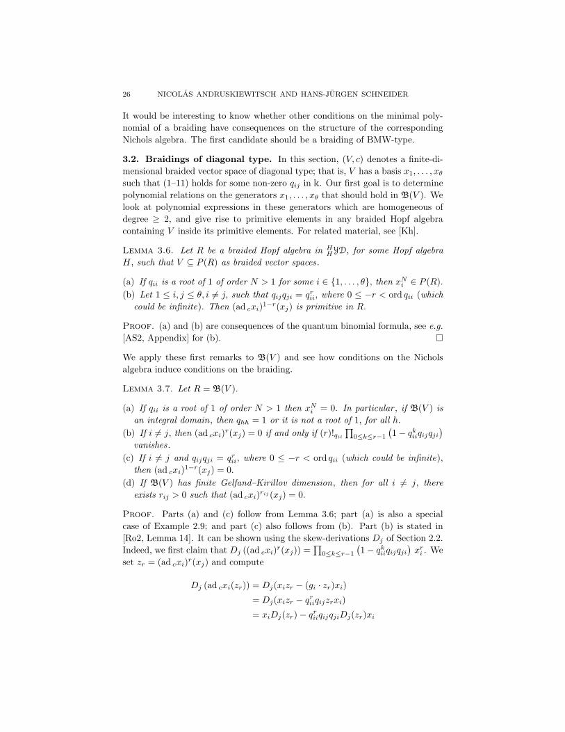
3.2. Braidings of diagonal type. In this section, (V, c) denotes a finite-di-mensional braided vector space of diagonal type; that is, V has a basis x1, . . . , xθ

such that (1–11) holds for some non-zero qij in k. Our first goal is to determinepolynomial relations on the generators x1, . . . , xθ that should hold in B(V ). Welook at polynomial expressions in these generators which are homogeneous ofdegree ≥ 2, and give rise to primitive elements in any braided Hopf algebracontaining V inside its primitive elements. For related material, see [Kh].

Lemma 3.6. Let R be a braided Hopf algebra in HHYD, for some Hopf algebra

H, such that V ⊆ P (R) as braided vector spaces.

(a) If qii is a root of 1 of order N > 1 for some i ∈ {1, . . . , θ}, then xNi ∈ P (R).

(b) Let 1 ≤ i, j ≤ θ, i 6= j, such that qijqji = qrii, where 0 ≤ −r < ord qii (which

could be infinite). Then (ad cxi)1−r(xj) is primitive in R.

Proof. (a) and (b) are consequences of the quantum binomial formula, see e.g.[AS2, Appendix] for (b). ¤

We apply these first remarks to B(V ) and see how conditions on the Nicholsalgebra induce conditions on the braiding.

Lemma 3.7. Let R = B(V ).

(a) If qii is a root of 1 of order N > 1 then xNi = 0. In particular , if B(V ) is

an integral domain, then qhh = 1 or it is not a root of 1, for all h.(b) If i 6= j, then (ad cxi)r(xj) = 0 if and only if (r)!qii

∏0≤k≤r−1

(1− qk

iiqijqji

)vanishes.

(c) If i 6= j and qijqji = qrii, where 0 ≤ −r < ord qii (which could be infinite),

then (ad cxi)1−r(xj) = 0.(d) If B(V ) has finite Gelfand–Kirillov dimension, then for all i 6= j, there

exists rij > 0 such that (ad cxi)rij (xj) = 0.

Proof. Parts (a) and (c) follow from Lemma 3.6; part (a) is also a specialcase of Example 2.9; and part (c) also follows from (b). Part (b) is stated in[Ro2, Lemma 14]. It can be shown using the skew-derivations Dj of Section 2.2.Indeed, we first claim that Dj ((ad cxi)r(xj)) =

∏0≤k≤r−1

(1− qk

iiqijqji

)xr

i . Weset zr = (ad cxi)r(xj) and compute

Dj (ad cxi(zr)) = Dj(xizr − (gi · zr)xi)

= Dj(xizr − qriiqijzrxi)

= xiDj(zr)− qriiqijqjiDj(zr)xi


and the claim follows by induction. Thus, by Example 2.9, Dj ((ad cxi)r(xj)) = 0if and only if (r)!qii

∏0≤k≤r−1

(1− qk

iiqijqji

)= 0. We next claim that

Di ((ad cxi)r(xj)) = 0.

We compute

Di (ad cxi(zr)) = Di(xizr − (gi · zr)xi)

= xiDi(zr) + gi · zr − gi · zr −Di(gi · zr) gi · xi

and the claim follows by induction. Finally, it is clear that Dl ((ad cxi)r(xj)) = 0,for all l 6= i, j. Part (b) follows then from Proposition 2.8.

Part(d) is an important result of Rosso [Ro2, Lemma 20]. ¤

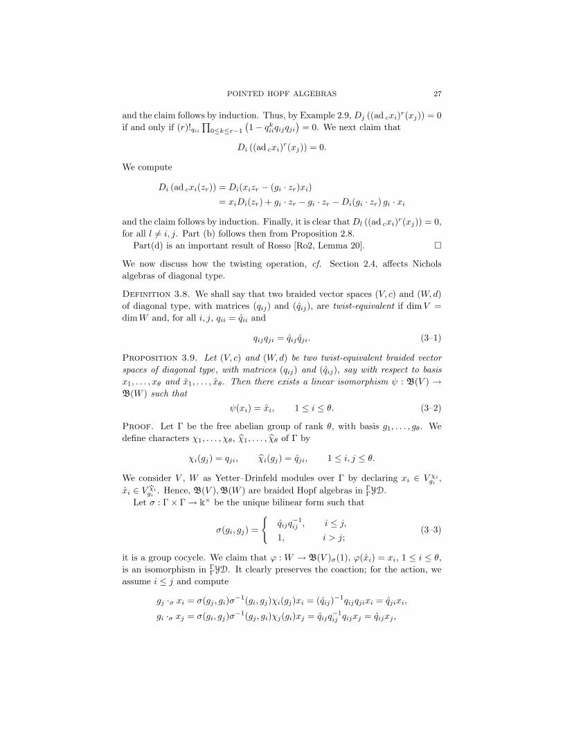
We now discuss how the twisting operation, cf. Section 2.4, affects Nicholsalgebras of diagonal type.

Definition 3.8. We shall say that two braided vector spaces (V, c) and (W,d)of diagonal type, with matrices (qij) and (qij), are twist-equivalent if dim V =dim W and, for all i, j, qii = qii and

qijqji = qij qji. (3–1)

Proposition 3.9. Let (V, c) and (W,d) be two twist-equivalent braided vectorspaces of diagonal type, with matrices (qij) and (qij), say with respect to basisx1, . . . , xθ and x1, . . . , xθ. Then there exists a linear isomorphism ψ : B(V ) →B(W ) such that

ψ(xi) = xi, 1 ≤ i ≤ θ. (3–2)

Proof. Let Γ be the free abelian group of rank θ, with basis g1, . . . , gθ. Wedefine characters χ1, . . . , χθ, χ1, . . . , χθ of Γ by

χi(gj) = qji, χi(gj) = qji, 1 ≤ i, j ≤ θ.

We consider V , W as Yetter–Drinfeld modules over Γ by declaring xi ∈ V χigi

,xi ∈ V bχi

gi. Hence, B(V ), B(W ) are braided Hopf algebras in Γ

ΓYD.Let σ : Γ× Γ → k× be the unique bilinear form such that

σ(gi, gj) =

{qijq

−1ij , i ≤ j,

1, i > j;(3–3)

it is a group cocycle. We claim that ϕ : W → B(V )σ(1), ϕ(xi) = xi, 1 ≤ i ≤ θ,is an isomorphism in Γ

ΓYD. It clearly preserves the coaction; for the action, weassume i ≤ j and compute

gj ·σ xi = σ(gj , gi)σ−1(gi, gj)χi(gj)xi = (qij)−1qijqjixi = qjixi,

gi ·σ xj = σ(gi, gj)σ−1(gj , gi)χj(gi)xj = qijq−1ij qijxj = qijxj ,


where we have used (2–12) and the hypothesis (3–1). This proves the claim. ByProposition 2.2, ϕ extends to an isomorphism ϕ : B(W ) → B(V )σ; ψ = ϕ−1 isthe map we are looking for. ¤

Remarks 3.10. (i) The map ψ defined in the proof is much more than justlinear; by (2–11) and (2–14), we have for all g, h ∈ Γ,

ψ(xy) = σ−1(g, h)ψ(x)ψ(y), x ∈ B(V )g, y ∈ B(V )h; (3–4)

ψ([x, y]c) = σ−1(g, h)[ψ(x), ψ(y)]d, x ∈ B(V )χg , y ∈ B(V )η

h. (3–5)

(ii) A braided vector space (V, c) of diagonal type, with matrix (qij), is twist-equivalent to (W,d), with a symmetric matrix (qij).

Twisting is a very important tool. For many problems, twisting allows to reduceto the case when the diagonal braiding is symmetric; then the theory of quantumgroups can be applied.

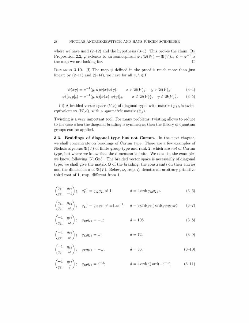
3.3. Braidings of diagonal type but not Cartan. In the next chapter,we shall concentrate on braidings of Cartan type. There are a few examples ofNichols algebras B(V ) of finite group type and rank 2, which are not of Cartantype, but where we know that the dimension is finite. We now list the exampleswe know, following [N; Gn3]. The braided vector space is necessarily of diagonaltype; we shall give the matrix Q of the braiding, the constraints on their entriesand the dimension d of B(V ). Below, ω, resp. ζ, denotes an arbitrary primitivethird root of 1, resp. different from 1.

(q11 q12

q21 −1

); q−1

11 = q12q21 6= 1; d = 4 ord(q12q21). (3–6)

(q11 q12

q21 ω

); q−1

11 = q12q21 6= ±1, ω−1; d = 9 ord(q11) ord(q12q21ω). (3–7)

(−1 q12

q21 ω

); q12q21 = −1; d = 108. (3–8)

(−1 q12

q21 ω

); q12q21 = ω; d = 72. (3–9)

(−1 q12

q21 ω

); q12q21 = −ω; d = 36. (3–10)

(−1 q12

q21 ζ

); q12q21 = ζ−2; d = 4 ord(ζ) ord(−ζ−1). (3–11)


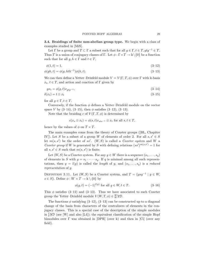
3.4. Braidings of finite non-abelian group type. We begin with a class ofexamples studied in [MiS].

Let Γ be a group and T ⊂ Γ a subset such that for all g ∈ Γ, t ∈ T, gtg−1 ∈ T .Thus T is a union of conjugacy classes of Γ. Let φ : Γ×T → k\{0} be a functionsuch that for all g, h ∈ Γ and t ∈ T ,

φ(1, t) = 1, (3–12)

φ(gh, t) = φ(g, hth−1)φ(h, t). (3–13)

We can then define a Yetter–Drinfeld module V = V (Γ, T, φ) over Γ with k-basisxt, t ∈ T, and action and coaction of Γ given by

gxt = φ(g, t)xgtg−1 , (3–14)

δ(xt) = t⊗ xt (3–15)

for all g ∈ Γ, t ∈ T .Conversely, if the function φ defines a Yetter–Drinfeld module on the vector

space V by (3–14), (3–15), then φ satisfies (3–12), (3–13).Note that the braiding c of V (Γ, T, φ) is determined by

c(xs ⊗ xt) = φ(s, t)xsts−1 ⊗ xt for all s, t ∈ T,

hence by the values of φ on T × T .

The main examples come from the theory of Coxeter groups ([BL, ChapitreIV]). Let S be a subset of a group W of elements of order 2. For all s, s′ ∈ S

let m(s, s′) be the order of ss′. (W,S) is called a Coxeter system and W aCoxeter group if W is generated by S with defining relations (ss′)m(s,s′) = 1 forall s, s′ ∈ S such that m(s, s′) is finite.

Let (W,S) be a Coxeter system. For any g ∈ W there is a sequence (s1, . . . , sq)of elements in S with g = s1 · · · · · sq. If q is minimal among all such represen-tations, then q = l(g) is called the length of g, and (s1, . . . , sq) is a reducedrepresentation of g.

Definition 3.11. Let (W,S) be a Coxeter system, and T = {gsg−1 | g ∈ W,

s ∈ S}. Define φ : W × T → k \ {0} by

φ(g, t) = (−1)l(g) for all g ∈ W, t ∈ T. (3–16)

This φ satisfies (3–12) and (3–13). Thus we have associated to each Coxetergroup the Yetter–Drinfeld module V (W,T, φ) ∈ W

W YD.

The functions φ satisfying (3–12), (3–13) can be constructed up to a diagonalchange of the basis from characters of the centralizers of elements in the con-jugacy classes. This is a special case of the description of the simple modulesin Γ

ΓYD (see [W] and also [L4]); the equivalent classification of the simple Hopfbimodules over Γ was obtained in [DPR] (over k) and then in [Ci] (over anyfield).


Let t be an element in Γ. We denote by Ot and Γt the conjugacy class andthe centralizer of t in Γ. Let U be any left kΓt-module. It is easy to see that theinduced representation V = kΓ⊗kΓt U is a Yetter–Drinfeld module over Γ withthe induced action of Γ and the coaction

δ : V → kΓ⊗ V, δ(g ⊗ u) = gtg−1 ⊗ g ⊗ u for all g ∈ Γ, u ∈ U.

We will denote this Yetter–Drinfeld module over Γ by M(t, U).Assume that Γ is finite. Then V = M(t, U) is a simple Yetter–Drinfeld module

if U is a simple representation of Γt, and each simple module in ΓΓYD has this

form. If we take from each conjugacy class one element t and non-isomorphicsimple Γt-modules, any two of these simple Yetter–Drinfeld modules are non-isomorphic.

Let si, 1 ≤ i ≤ θ, be a complete system of representatives of the residueclasses of Γt. We define ti = sits

−1i for all 1 ≤ i ≤ θ. Thus

Γ/Γt → Ot, siΓt 7→ ti, 1 ≤ i ≤ θ,

is bijective, and as a vector space, V =⊕

1≤i≤θ si ⊗ U . For all g ∈ Γ and1 ≤ i ≤ θ, there is a uniquely determined 1 ≤ j ≤ θ with s−1

j gsi ∈ Γt, and theaction of g on si ⊗ u, u ∈ U , is given by

g(si ⊗ u) = sj ⊗ (s−1j gsi)u.

In particular, if U is a one-dimensional Γt-module with basis u and action hu =χ(h)u for all h ∈ Γt defined by the character χ : Γt → k \ {0}, then V has abasis xi = si ⊗ u, 1 ≤ i ≤ θ, and the action and coaction of Γ are given by

gxi = χ(s−1j gsi)xj and δ(xi) = ti ⊗ xi,

if s−1j gsi ∈ Γt. Note that gtig

−1 = tj . Hence the module we have constructedis V (Γ, T, φ), where T is the conjugacy class of t, and φ is given by φ(g, ti) =χ(s−1

j gsi).

We now construct another example of a function φ satisfying (3–12), (3–13).

Definition 3.12. Let T be the set of all transpositions in the symmetric groupSn. Define φ : Sn × T → k \ {0} for all g ∈ Sn, 1 ≤ i < j ≤ n, by

φ(g, (ij)) =

{1 , if g(i) < g(j),

−1 , if g(i) > g(j).(3–17)

Let t = (12). The centralizer of t in Sn is

〈(34), (45), . . . , (n−1, n)〉 ∪ 〈(34), (45), . . . , (n−1, n)〉(12).

Let χ be the character of (Sn)t with χ((ij)) = 1 for all 3 ≤ i < j ≤ n, andχ((12)) = −1. Then the function φ defined by (3–17) is given by the characterχ as described above.


Up to base change we have found all functions φ satisfying (3–12), (3–13) forΓ = Sn, where T is the conjugacy class of all transpositions, and φ(t, t) = −1for all t ∈ T . The case φ(t, t) = 1 for some t ∈ T would lead to a Nichols algebraB(V ) of infinite dimension.

To determine the structure of B(V ) for the Yetter–Drinfeld modules definedby the functions φ in (3–16) and (3–17) seems to be a fundamental and veryhard combinatorial problem. Only a few partial results are known [MiS], [FK],[FP].

We consider some special cases; here the method of skew-derivations is applied,see Proposition 2.8.

Example 3.13. Let W = Sn, n ≥ 2, and T = {(ij) | 1 ≤ i < j ≤ n} theset of all transpositions. Define φ by (3–16) and let V = V (W,T, φ). Then thefollowing relations hold in B(V ) for all 1 ≤ i < j ≤ n, 1 ≤ k < l ≤ n:

x2(ij) = 0. (3–18)

If {i, j} ∩ {k, l} = ∅, then x(ij)x(kl) + x(kl)x(ij) = 0. (3–19)

If i < j < k, then x(ij)x(jk) + x(jk)x(ik) + x(ik)x(ij) = 0, (3–20)

x(jk)x(ij) + x(ik)x(jk) + x(ij)x(ik) = 0.

Example 3.14. Let W = Sn, n ≥ 2, and T = {(ij) | 1 ≤ i < j ≤ n} theset of all transpositions. Define φ by (3–17) and let V = V (W,T, φ). Then thefollowing relations hold in B(V ) for all 1 ≤ i < j ≤ n, 1 ≤ k < l ≤ n:

x2(ij) = 0. (3–21)

If {i, j} ∩ {k, l} = ∅, then x(ij)x(kl) − x(kl)x(ij) = 0. (3–22)

If i < j < k, then x(ij)x(jk) − x(jk)x(ik) − x(ik)x(ij) = 0, (3–23)

x(jk)x(ij) − x(ik)x(jk) − x(ij)x(ik) = 0.

The algebras B(V ) generated by all x(ij), 1 ≤ i < j ≤ n, with the quadraticrelations in the examples 3.13 resp. 3.14 are braided Hopf algebras in the categoryof Yetter–Drinfeld modules over Sn. B(V ) in example 3.14 is the algebra En

introduced by Fomin and Kirillov in [FK] to describe the cohomology ring of theflag variety. We believe that indeed the quadratic relations in the examples 3.13and 3.14 are defining relations for B(V ), that is B(V ) = B(V ) in these cases.

It was noted in [MiS] that the conjecture in [FK] about the ”Poincare-duality“of the dimensions of the homogeneous components of the algebras En (in casethey are finite-dimensional) follows from the braided Hopf algebra structure asa special case of Lemma 1.12.

Another result about the algebras En by Fomin and Procesi [FP] says thatEn+1 is a free module over En, and PEn divides PEn+1 , where PA denotes theHilbert series of a graded algebra A. The proof in [FP] used the relations inExample 3.14.


This result is in fact a special case of a very general splitting theorem forbraided Hopf algebras in [MiS, Theorem3.2] which is an application of the fun-damental theorem for Hopf modules in the braided situation. This splittingtheorem generalizes the main result of [Gn2].

In [MiS] some partial results are obtained about the structure of the Nicholsalgebras of Coxeter groups. In particular

Theorem 3.15. [MiS, Corollary 5.9]Let (W,S) be a Coxeter system, T theset of all W -conjugates of elements in S, φ defined by (3–16), V = V (W,T, φ)and R = B(V ). For all g ∈ W , choose a reduced representation g = s1 · · · sq,s1, · · · , sq ∈ S, of g, and define

xg = xs1 · · ·xsq .

Then the subalgebra of R generated by all xs, s ∈ S has the k-basis xg, g ∈ W .For all g ∈ W , the g-homogeneous component Rg of R is isomorphic to R1.

If R is finite-dimensional , then W is finite and dim(R) = ord(W )dim(R1).

This theorem holds for more general functions φ, in particular for Sn and φ

defined in (3–17).

Let (W,S) be a Coxeter system and V = V (W,T, φ) as in Theorem [MiS].Then B(V ) was computed in [MiS] in the following cases:

• W = S3, S = {(12), (23)}: The relations of B(V ) are the quadratic relationsin Example 3.13, and dim B(V ) = 12.

• W = S4, S = {(12), (23), (34)}: The relations of B(V ) are the quadraticrelations in Example 3.13, and dimB(V ) = 24 · 24.

• W = D4, the dihedral group of order 8, S = {t, t′}, where t, t′ are generatorsof D4 of order 2 such that tt′ is of order 4. There are quadratic relations andrelations of order 4 defining B(V ), and dim B(V ) = 64.

In all three cases the integral, which is the longest non-zero word in the generatorsxt, can be described in terms of the longest element in the Coxeter group. In allthe other cases it is not known whether B(V ) is finite-dimensional.

In [FK] it is shown that

• dim(E3) = 12.

• dim(E4) = 24 · 24.

• dim(E5) is finite by using a computer program.

Again, for the other cases n > 5 it is not known whether En is finite-dimensional.

In [Gn3, 5.3.2] another example of a finite-dimensional Nichols algebra of abraided vector space (V, c) of finite group type is given with dim(V ) = 4 anddim(B(V )) = 72. The defining relations of B(V ) are quadratic and of order 6.


By a result of Montgomery [M2], any pointed Hopf algebra B can be decom-posed as a crossed product

B ' A#σkG, σ a 2-cocycle

of A, its link-indecomposable component containing 1 (a Hopf subalgebra) anda group algebra kG. However, the structure of such link-indecomposable Hopfalgebras A, in particular in the case when A is finite-dimensional and the groupof its group-like elements G(A) is non-abelian, is not known. To define link-indecomposable pointed Hopf algebras, we recall the definition of the quiver of A

in [M2]. The vertices of the quiver of A are the elements of the group G(A); forg, h ∈ G(A), there exists an arrow from h to g if Pg,h(A) is non-trivial, that isif k(g − h) $ Pg,h(A). The Hopf algebra A is called link-indecomposable, if itsquiver is connected as an undirected graph.

Definition 3.16. Let Γ be a finite group and V ∈ ΓΓYD. V is called link-

indecomposable if the group Γ is generated by the elements g with Vg 6= 0.

By [MiS, 4.2], V ∈ ΓΓYD is link-indecomposable if and only if the Hopf algebra

B(V )#kΓ is link-indecomposable.Thus, by the examples constructed above, there are link-indecomposable,

finite-dimensional pointed Hopf algebras A with G(A) isomorphic to Sn, 3 ≤n ≤ 5, or to D4.

Question 3.17. Which finite groups are isomorphic to G(A) for some finite-dimensional, link-indecomposable pointed Hopf algebra A? Are there finitegroups which do not occur in this form?

Finally, let us come back to the simple Yetter–Drinfeld modules V = M(t, U) ∈ΓΓYD, where t ∈ Γ and U is a simple left Γt-module of dimension > 1. In thiscase, strong restrictions are known for B(V ) to be finite-dimensional. By Schur’slemma, t acts as a scalar q on U .

Proposition 3.18. [Gn3, 3.1] Assume that dim B(V ) is finite. If dim U ≥ 3,then q = −1; and if dim U = 2, then q = −1 or q is a root of unity of orderthree.

In the proof of Proposition 3.18, a result of Lusztig on braidings of Cartan type(see [AS2, Theorem 3.1]) is used. In a similar way Grana showed

Proposition 3.19. [Gn3, 3.2] Let Γ be a finite group of odd order , and V ∈ΓΓYD. Assume that B(V ) is finite-dimensional . Then the multiplicity of anysimple Yetter–Drinfeld module over Γ as a direct summand in V is at most 2.

In particular , up to isomorphism there are only finitely many Yetter–Drinfeldmodules V ∈ Γ

ΓYD such that B(V ) is finite-dimensional .

The second statement in Proposition 3.19 was a conjecture in a preliminaryversion of [AS2].


3.5. Braidings of (infinite) group type. We briefly mention Nichols algebrasover a free abelian group of finite rank with a braiding which is not diagonal.

Example 3.20. Let Γ = 〈g〉 be a free group in one generator. Let V(t, 2) bethe Yetter–Drinfeld module of dimension 2 such that V(t, 2) = V(t, 2)g and theaction of g on V(t, 2) is given, in a basis x1, x2, by

g · x1 = tx1, g · x2 = tx2 + x1.

Here t ∈ k×. Then:(a) If t is not a root of 1, then B(V(t, 2)) = T (V(t, 2)).(b) If t = 1, then B(V(1, 2)) = k〈x1, x2|x1x2 = x2x1 + x2

1〉; this is the well-known Jordanian quantum plane.

Example 3.21. More generally, if t ∈ k×, let V(t, θ) be the Yetter–Drinfeldmodule of dimension θ ≥ 2 such that V(t, θ) = V(t, θ)g and the action of g onV(t, θ) is given, in a basis x1, . . . , xθ, by

g · x1 = tx1, g · xj = txj + xj−1, 2 ≤ j ≤ θ.

Note there is an inclusion of Yetter–Drinfeld modules V(t, 2) ↪→ V(t, θ); hence,if t is not a root of 1, B(V(t, θ)) has exponential growth.

Question 3.22. Compute B(V(1, θ)); does it have finite growth?

4. Nichols Algebras of Cartan Type

We now discuss fundamental examples of Nichols algebras of diagonal typethat come from the theory of quantum groups.

We first need to fix some notation. Let A = (aij)1≤i,j≤θ be a generalizedsymmetrizable Cartan matrix [K]; let (d1, . . . , dθ) be positive integers such thatdiaij = djaji. Let g be the Kac–Moody algebra corresponding to the Cartanmatrix A. Let X be the set of connected components of the Dynkin diagramcorresponding to it. For each I ∈ X, we let gI be the Kac–Moody Lie algebracorresponding to the generalized Cartan matrix (aij)i,j∈I and nI be the Liesubalgebra of gI spanned by all its positive roots. We omit the subindex I whenI = {1, . . . , θ}. We assume that for each I ∈ X, there exist cI , dI such thatI = {j : cI ≤ j ≤ dI}; that is, after reordering the Cartan matrix is a matrixof blocks corresponding to the connected components. Let I ∈ X and i ∼ j inI; then Ni = Nj , hence NI := Ni is well defined. Let ΦI , resp. Φ+

I , be the rootsystem, resp. the subset of positive roots, corresponding to the Cartan matrix(aij)i,j∈I ; then Φ =

⋃I∈X ΦI , resp. Φ+ =

⋃I∈X Φ+

I is the root system, resp. thesubset of positive roots, corresponding to the Cartan matrix (aij)1≤i,j≤θ. Letα1, . . . , αθ be the set of simple roots.

Let WI be the Weyl group corresponding to the Cartan matrix (aij)i,j∈I ; weidentify it with a subgroup of the Weyl group W corresponding to the Cartanmatrix (aij).


If (aij) is of finite type, we fix a reduced decomposition of the longest elementω0,I of WI in terms of simple reflections. Then we obtain a reduced decompo-sition of the longest element ω0 = si1 . . . siP

of W from the expression of ω0 asproduct of the ω0,I ’s in some fixed order of the components, say the order arisingfrom the order of the vertices. Therefore βj := si1 . . . sij−1(αij ) is a numerationof Φ+.

Example 4.1. Let q ∈ k, q 6= 0, and consider the braided vector space (V, c),where V is a vector space with a basis x1, . . . , xθ and the braiding c is given by

c(xi ⊗ xj) = qdiaij xj ⊗ xi, (4–1)

Theorem 4.2. [L3, 33.1.5] Let (V, c) be a braided vector space with braidingmatrix (4–1). If q is not algebraic over Q, then

B(V) = k〈x1, . . . , xθ|ad c(xi)1−aij xj = 0, i 6= j〉.The theorem says that B(V) is the well-known “positive part” U+

q (g) of theDrinfeld–Jimbo quantum enveloping algebra of g.

To state the following important theorem, we recall the definition of braidedcommutators (1–20). Lusztig defined root vectors Xα ∈ B(V), α ∈ Φ+ [L2].One can see from [L1; L2] that, up to a non-zero scalar, each root vector canbe written as an iterated braided commutator in some sequence Xl1 , . . . , Xla ofsimple root vectors such as [[Xl1 , [Xl2 , Xl3 ]c]c, [Xl4 , Xl5 ]c]c. See also [Ri].

Theorem 4.3 [L1; L2; L3; dCP; Ro1; Mu]. Let (V, c) be a braided vector spacewith braiding matrix (4–1). Assume that q is a root of 1 of odd order N ; andthat 3 does not divide N if there exists I ∈ X of type G2.

The algebra B(V) is finite-dimensional if and only if (aij) is a finite Cartanmatrix .

If this happens, then B(V) can be presented by generators Xi, 1 ≤ i ≤ θ, andrelations

ad c(Xi)1−aij (Xj) = 0, i 6= j, (4–2)

XNα = 0, α ∈ Φ+. (4–3)

Moreover , the following elements constitute a basis of B(V):

Xh1β1

Xh2β2

. . . XhP

βP, 0 ≤ hj ≤ N − 1, 1 ≤ j ≤ P.

The theorem says that B(V) is the well-known “positive part” u+q (g) of the

so-called Frobenius–Lusztig kernel of g.Motivated by the preceding theorems and results, we introduce the following

notion, generalizing [AS2] (see also [FG]).

Definition 4.4. Let (V, c) a braided vector space of diagonal type with basisx1, . . . , xθ, and matrix (qij), that is

c(xi ⊗ xj) = qi,jxj ⊗ xi, for all 1 ≤ i, j ≤ θ.


We shall say that (V, c) is of Cartan type if qii 6= 1 for all i, and there are integersaij with aii = 2, 1 ≤ i ≤ θ, and 0 ≤ −aij < ord qii (which could be infinite),1 ≤ i 6= j ≤ θ, such that

qijqji = qaij

ii , 1 ≤ i, j ≤ θ.

Since clearly aij = 0 implies that aji = 0 for all i 6= j, (aij) is a generalizedCartan matrix in the sense of the book [K]. We shall adapt the terminology fromgeneralized Cartan matrices and Dynkin diagrams to braidings of Cartan type.For instance, we shall say that (V, c) is of finite Cartan type if it is of Cartantype and the corresponding GCM is actually of finite type, i.e. a Cartan matrixassociated to a finite-dimensional semisimple Lie algebra. We shall say that aYetter–Drinfeld module V is of Cartan type if the matrix (qij) as above is ofCartan type.

Definition 4.5. Let (V, c) be a braided vector space of Cartan type with Cartanmatrix (aij). We say that (V, c) is of FL-type (or Frobenius–Lusztig type) if thereexist positive integers d1, . . . , dθ such that

For all i, j, diaij = djaji (thus (aij) is symmetrizable). (4–4)

There exists a root of unity q ∈ k such that qij = qdiaij for all i, j. (4–5)

We call (V, c) locally of FL-type if any principal 2× 2 submatrix of (qij) definesa braiding of FL-type.

We now fix for each α ∈ Φ+ such a representation of Xα as an iterated braidedcommutator. For a general braided vector space (V, c) of finite Cartan type,we define root vectors xα in the tensor algebra T (V ), α ∈ Φ+, as the sameformal iteration of braided commutators in the elements x1, . . . , xθ instead ofX1, . . . , Xθ but with respect to the braiding c given by the general matrix (qij).

Theorem 4.6. [AS2, Th. 1.1], [AS4, Th. 4.5]. Let (V, c) be a braided vectorspace of Cartan type. We also assume that qij has odd order for all i, j.

(i) Assume that (V, c) is locally of FL-type and that , for all i, the order of qii isrelatively prime to 3 whenever aij = −3 for some j, and is different from 3,5, 7, 11, 13, 17. If B(V ) is finite-dimensional , then (V, c) is of finite Cartantype.

(ii) If (V, c) is of finite Cartan type, then B(V ) is finite dimensional , and ifmoreover 3 does not divide the order of qii for all i in a connected componentof the Dynkin diagram of type G2, then

dim B(V ) =∏

I∈X

Ndim nI

I ,


where NI = ord(qii) for all i ∈ I and I ∈ X. The Nichols algebra B(V ) ispresented by generators xi, 1 ≤ i ≤ θ, and relations

ad c(xi)1−aij (xj) = 0, i 6= j, (4–6)

xNIα = 0, α ∈ Φ+

I , I ∈ X. (4–7)

Moreover , the following elements constitute a basis of B(V ):

xh1β1

xh2β2

. . . xhP

βP, 0 ≤ hj ≤ NI − 1, if βj ∈ I, 1 ≤ j ≤ P.

Let B(V ) be the braided Hopf algebra in ΓΓYD generated by x1, . . . , xθ with

relations (4–6), where the xi’s are primitive. Let K(V ) be the subalgebra ofB(V ) generated by xNI

α , α ∈ Φ+I , I ∈ X; it is a Yetter–Drinfeld submodule of

B(V ).

Theorem 4.7. [AS4, Th. 4.8] K(V ) is a braided Hopf subalgebra in ΓΓYD of

B(V ).

5. Classification of Pointed Hopf Algebras by the LiftingMethod

5.1. Lifting of Cartan type. We propose subdividing the classification prob-lem for finite-dimensional pointed Hopf algebras into the following problems:

(a) Determine all braided vector spaces V of group type such that B(V ) isfinite-dimensional.

(b) Given a finite group Γ, determine all realizations of braided vector spaces V

as in (a) as Yetter–Drinfeld modules over Γ.(c) The lifting problem: For V as in (b), compute all Hopf algebras A such that

gr A ' B(V )#H .(d) Investigate whether any finite-dimensional pointed Hopf algebra is generated

as an algebra by its group-like and skew-primitive elements.

Problem (a) was discussed in Chapters 3 and 4. We have seen the very importantclass of braidings of finite Cartan type and some isolated examples where theNichols algebra is finite-dimensional. But the general case of problem (a) seemsto require completely new ideas.

Problem (b) is of a computational nature. For braidings of finite Cartan typewith Cartan matrix (aij)1≤i,j≤θ and an abelian group Γ we have to computeelements g1, . . . , gθ ∈ Γ and characters χ1, . . . , χθ ∈ Γ such that

χi(gj)χj(gi) = χi(gi)aij , for all 1 ≤ i, j ≤ θ. (5–1)

To find these elements one has to solve a system of quadratic congruences in sev-eral unknowns. In many cases they do not exist. In particular, if θ > 2(ordΓ)2,then the braiding cannot be realized over the group Γ. We refer to [AS2, Section8] for details.


Problem (d) is the subject of Section 5.4.

We will now discuss the lifting problem (c).The coradical filtration kΓ = A0 ⊂ A1 ⊂ · · · of a pointed Hopf algebra A is

stable under the adjoint action of the group. For abelian groups Γ and finite-dimensional Hopf algebras, the following stronger result holds. It is the startingpoint of the lifting procedure, and we will use it several times.

If M is a kΓ-module, we denote by Mχ = {m ∈ M | gm = χ(g)m for all g ∈Γ}, χ ∈ Γ, the isotypic component of type χ.

Lemma 5.1. Let A be a finite-dimensional Hopf algebra with abelian groupG(A) = Γ and diagram R. Let V = R(1) ∈ Γ

ΓYD with basis xi ∈ V χigi

, gi ∈Γ, χi ∈ Γ, 1 ≤ i ≤ θ.

(a) The isotypic component of trivial type of A1 is A0. Therefore, A1 =A0 ⊕ (

⊕χ 6=ε(A1)χ) and

⊕

χ6=ε

(A1)χ '−→ A1/A0'←− V #kΓ. (5–2)

(b) For all g ∈ Γ, χ ∈ Γ with χ 6= ε,

Pg,1(A)χ 6= 0 ⇐⇒ there is some 1 ≤ l ≤ θ : g = gl, χ = χl; (5–3)

Pg,1(A)ε = k(1− g). (5–4)

Proof. (a) follows from [AS1, Lemma 3.1] and implies (b). See [AS1, Lemma5.4]. ¤

We assume that A is a finite-dimensional pointed Hopf algebra with abeliangroup G(A) = Γ, and that

gr A ' B(V )#kΓ,

where V ∈ ΓΓYD is a given Yetter–Drinfeld module with basis xi∈V χi

gi, g1 . . . , gθ ∈

Γ, χ1, . . . , χθ ∈ Γ, 1 ≤ i ≤ θ.

We first lift the basis elements xi. Using (5–2), we choose ai ∈ P(A)χi

gi,1such

that the canonical image of ai in A1/A0 is xi (which we identify with xi#1),1 ≤ i ≤ θ. Since the elements xi together with Γ generate B(V )#kΓ, it followsfrom a standard argument that a1, . . . , aθ and the elements in Γ generate A asan algebra.

Our aim is to find relations between the a′is and the elements in Γ which definea quotient Hopf algebra of the correct dimension dimB(V ) · ord(Γ). The idea isto ”lift“ the relations between the x′is and the elements in Γ in B(V )#kΓ.

We now assume moreover that V is of finite Cartan type with Cartan matrix(aij) with respect to the basis x1, . . . , xθ, that is (5–1) holds. We also assume

ord(χj(gi)) is odd for all i, j, (5–5)

Ni = ord(χi(gi)) is prime to 3 for all i ∈ I, I ∈ X of type G2. (5–6)


We fix a presentation Γ = 〈y1〉⊕ · · · ⊕ 〈yσ〉, and denote by Ml the order of yl,1 ≤ l ≤ σ. Then Theorem 4.6 and formulas (1–17) imply that B(V )#kΓ can bepresented by generators hl, 1 ≤ l ≤ σ, and xi, 1 ≤ i ≤ θ with defining relations

hMl

l = 1, 1 ≤ l ≤ σ; (5–7)

hlht = hthl, 1 ≤ t < l ≤ σ; (5–8)

hlxi = χi(yl)xihl, 1 ≤ l ≤ σ, 1 ≤ i ≤ θ; (5–9)

xNIα = 0, α ∈ Φ+

I , I ∈ X; (5–10)

ad (xi)1−aij (xj) = 0, i 6= j, (5–11)

and where the Hopf algebra structure is determined by

∆(hl) = hl ⊗ hl, 1 ≤ l ≤ σ; (5–12)

∆(xi) = xi ⊗ 1 + gi ⊗ xi, 1 ≤ i ≤ θ. (5–13)

Thus A is generated by the elements ai, 1 ≤ i ≤ θ, and hl, 1 ≤ l ≤ σ. Byour previous choice, relations (5–7), (5–8), (5–9) and (5–12), (5–13) all hold inA with the x′is replaced by the a′is.

The remaining problem is to lift the quantum Serre relations (5–11) and theroot vector relations (5–10). We will do this in the next two Sections.

5.2. Lifting the quantum Serre relations. We divide the problem into twocases.

• Lifting of the “quantum Serre relations” xixj − χj(gi)xjxi = 0, when i 6= j

are in different components of the Dynkin diagram.• Lifting of the “quantum Serre relations” ad c(xi)1−aij (xj) = 0, when i 6= j are

in the same component of the Dynkin diagram.

The first case is settled in the next result from [AS4, Theorem 6.8 (a)].

Lemma 5.2. Assume that 1 ≤ i, j ≤ θ, i < j and i 6∼ j. Then

aiaj − χj(gi)ajai = λij(1− gigj), (5–14)

where λij is a scalar in k which can be chosen such that

λij is arbitrary if gigj 6= 1 and χiχj = ε, but 0 otherwise. (5–15)

Proof. It is easy to check that aiaj − χj(gi)ajai ∈ P(A)χiχj

gigj ,1. Suppose thatχiχj 6= ε and aiaj − χj(gi)ajai 6= 0. Then by (5–3), χiχj = χl and gigj = gl forsome 1 ≤ l ≤ θ.

Substituting gl and χl in χi(gl)χl(gi) = χi(gi)ail and using χi(gj)χj(gi) = 1(since aij = 0, i and j lie in different components), we get χi(gi)2 = χi(gi)ail .


Thus we have shown that ail ≡ 2 mod Ni, and in the same way ajl ≡ 2mod Nj . Since i 6∼ j, ail or ajl must be 0, and we obtain the contradictionNi = 2 or Nj = 2.

Therefore χiχj = ε, and the claim follows from (5–4), or aiaj−χj(gi)ajai = 0,and the claim is trivial. ¤

Lemma 5.2 motivates the following notion.

Definition 5.3. [AS4, Definition 5.1] We say that two vertices i and j arelinkable (or that i is linkable to j) if

i 6∼ j, (5–16)

gigj 6= 1 and (5–17)

χiχj = ε. (5–18)

The following elementary properties are easily verified:

If i is linkable to j, then χi(gj)χj(gi) = 1, χj(gj) = χi(gi)−1. (5–19)

If i and k, resp. j and l, are linkable, then aij = akl, aji = alk. (5–20)

A vertex i can not be linkable to two different vertices j and h. (5–21)

A linking datum is a collection (λij)1≤i<j≤θ, i 6∼j of elements in k such that λij isarbitrary if i and j are linkable but 0 otherwise. Given a linking datum, we saythat two vertices i and j are linked if λij 6= 0.

The notion of a linking datum encodes the information about lifting of rela-tions in the first case.

Definition 5.4. The collection D formed by a finite Cartan matrix (aij), andg1, . . . , gθ ∈ Γ, χ1, . . . , χθ ∈ Γ satisfying (5–1), (5–5) and (5–6), and a linkingdatum (λij)1≤i<j≤θ, i 6∼j will be called a linking datum of finite Cartan type forΓ. We define the Yetter–Drinfeld module V ∈ Γ

ΓYD of D as the vector spacewith basis x1, . . . , xθ with xi ∈ V χi

gifor all i.

If D is a linking datum of finite Cartan type for Γ, we define the Hopf al-gebra u(D) by generators ai, 1 ≤ i ≤ θ, and hl, 1 ≤ l ≤ σ and the relations(5–7),(5–8),(5–9),(5–10), the quantum Serre relations (5–11) for i 6= j and i ∼ j,(5–12),(5–13) with the xi’s replaced by the ai’s, and the lifted quantum Serrerelations (5–14). We formally include the case when θ = 0 and u(D) is a groupalgebra.

In the definition of u(D) we could always assume that the linking datum con-tains only elements λij ∈ {0, 1} (by multiplying the generators ai with non-zeroscalars).

Theorem 5.5. [AS4, Th. 5.17] Let Γ be a finite abelian group and D a linkingdatum of finite Cartan type for Γ with Yetter–Drinfeld module V . Then u(D) isa finite-dimensional pointed Hopf algebra with gr u(D) ' B(V )#kΓ.


The proof of the theorem is by induction on the number of irreducible com-ponents of the Dynkin diagram. In the induction step a new Hopf algebra isconstructed by twisting the multiplication of the tensor product of two Hopfalgebras by a 2-cocycle. The 2-cocycle is defined in terms of the linking datum.

Note that the Frobenius–Lusztig kernel uq(g) of a semisimple Lie algebra g

is a special case of u(D). Here the Dynkin diagram of D is the disjoint unionof two copies of the Dynkin diagram of g, and corresponding points are linkedpairwise. But many other linkings are possible, for example 4 copies of A3 linkedin a circle [AS4, 5.13]. See [D] for a combinatorial description of all linkings ofDynkin diagrams.

Let us now turn to the second case. Luckily it turns out that (up to somesmall order exceptions) in the second case the Serre relations simply hold in thelifted situation without any change.

Theorem 5.6. [AS4, Theorem 6.8]. Let I ∈ X. Assume that NI 6= 3. If I is oftype Bn, Cn or F4, resp. G2, assume further that NI 6= 5, resp. NI 6= 7. Thenthe quantum Serre relations hold for all i, j ∈ I, i 6= j, i ∼ j.

5.3. Lifting the root vector relations. Assume first that the root α issimple and corresponds to a vertex i. It is not difficult to see, using the quantumbinomial formula, that aNi

i is a (gNii , 1)-skew-primitive. By Lemma 5.1, we have

aNii = µi

(1− gNi

i

), (5–22)

for some scalar µi; this scalar can be chosen so that

µi is arbitrary if gNii 6= 1 and χNi

i = 1 but 0 otherwise. (5–23)

Now, if the root α is not simple then aNii is not necessarily a skew-primitive,

but a skew-primitive “modulo root vectors of shorter length”.In general, we define the root vector aα for α ∈ Φ+

I , I ∈ X, by replacing thexi by ai in the formal expression for xα as a braided commutator in the simpleroot vectors. Then aNI

α , α ∈ I, should be an element uα in the group algebra ofthe subgroup generated by the NI -th powers of the elements in Γ.

Finally, the Hopf algebra generated by ai, 1 ≤ i ≤ θ, and hl, 1 ≤ l ≤ σ withthe relations (5–7),(5–8),(5–9) (with ai instead of xi),

• the lifted root vector relations aNIα = uα, α ∈ Φ+

I , I ∈ X,• the quantum Serre relations (5–11) for i 6= j and i ∼ j (with ai instead of xi),• the lifted quantum Serre relations (5–14),

should have the correct dimension dim(B(V )) · ord(Γ).We carried out all the steps of this program in the following cases:

(a) All connected components of the Dynkin diagram are of type A1 [AS1].(b) The Dynkin diagram is of type A2, and N > 3 is odd [AS3].(c) The Dynkin diagram is arbitrary, but we assume gNi

i = 1 for all i [AS4].


(d) The Dynkin diagram is of type An, any n ≥ 2, and N > 3 , see Section 6 ofthis paper.

The cases A2, N = 3 and B2, N odd and 6= 5, were recently done in [BDR].Here N denotes the common order of χi(gi) for all i when the Dynkin diagramis connected.

5.4. Generation in degree one. Let us now discuss step (d) of the Liftingmethod.

It is not difficult to show that our conjecture 2.7 about Nichols algebras, inthe setting of H = kΓ, is equivalent to

Conjecture 5.7. [AS3]. Any pointed finite-dimensional Hopf algebra over k isgenerated by group-like and skew-primitive elements.

We have seen in Section 2.1 that the corresponding conjecture is false whenthe Hopf algebra is infinite-dimensional or when the Hopf algebra is finite-dimensional and the characteristic of the field is > 0. A strong indication thatthe conjecture is true is given by:

Theorem 5.8. [AS4, Theorem 7.6]. Let A be a finite-dimensional pointed Hopfalgebra with coradical kΓ and diagram R, that is

gr A ' R#kΓ.

Assume that R(1) is a Yetter–Drinfeld module of finite Cartan type with braiding(qij)1≤i,j≤θ. For all i , let qi = qii, Ni = ord(qi). Assume that ord(qij) is odd andNi is not divisible by 3 and > 7 for all 1 ≤ i, j ≤ θ.

(i) For any 1 ≤ i ≤ θ contained in a connected component of type Bn, Cn or F4

resp. G2, assume that Ni is not divisible by 5 resp. by 5 or 7.(ii) If i and j belong to different components, assume qiqj = 1 or ord(qiqj) = Ni.

Then R is generated as an algebra by R(1), that is A is generated by skew-primitive and group-like elements.

Let us discuss the idea of the proof of Theorem 5.8. At one decisive point, weuse our previous results about braidings of Cartan type of rank 2.

Let S be the graded dual of R. By the duality principle in Lemma 2.4, S isgenerated in degree one since P (R) = R(1). Our problem is to show that R isgenerated in degree one, that is S is a Nichols algebra.

Since S is generated in degree one, there is a surjection of graded braidedHopf algebras S → B(V ), where V = S(1) has the same braiding as R(1). Butwe know the defining relations of B(V ), since it is of finite Cartan type. So wehave to show that these relations also hold in S.

In the case of a quantum Serre relation ad c(xi)1−aij (xj)=0, i 6= j, we considerthe Yetter–Drinfeld submodule W of S generated by xi and ad c(xi)1−aij (xj) andassume that ad c(xi)1−aij (xj) 6= 0. The assumptions (1) and (2) of the theorem


guarantee that W also is of Cartan type, but not of finite Cartan type. Thusad c(xi)1−aij (xj) = 0 in S.

Since the quantum Serre relations hold in S, the root vector relations followautomatically from the next Lemma which is a consequence of Theorem 4.7.

Lemma 5.9. [AS4, Lemma 7.5] Let S =⊕

n≥0 S(n) be a finite-dimensionalgraded Hopf algebra in Γ

ΓYD such that S(0) = k1. Assume that V = S(1) is ofCartan type with basis (xi)1≤i,j≤θ as described in the beginning of this Section.Assume the Serre relations

(ad cxi)1−aij xj = 0 for all 1 ≤ i, j ≤ θ, i 6= j and i ∼ j.

Then the root vector relations

xNIα = 0, α ∈ Φ+

I , I ∈ X,

hold in S.

Another result supporting Conjecture 5.7 is:

Theorem 5.10. [AEG, 6.1] Any finite-dimensional cotriangular pointed Hopfalgebra is generated by skew-primitive and group-like elements.

5.5. Applications. As a special case of the theory explained above we obtaina complete answer to the classification problem in a significant case.

Theorem 5.11. [AS4, Th. 1.1] Let p be a prime > 17, s ≥ 1, and Γ = (Z/(p))s.Up to isomorphism there are only finitely many finite-dimensional pointed Hopfalgebras A with G(A) ' Γ. They all have the form

A ' u(D), where D is a linking datum of finite Cartan type for Γ.

If we really want to write down all these Hopf algebras we still have to solve thefollowing serious problems:

• Determine all Yetter–Drinfeld modules V over Γ = (Z/(p))s of finite Cartantype.

• Determine all the possible linkings for the modules V over (Z/(p))s in (a).

By [AS2, Proposition 8.3], dimV ≤ 2sp−1p−2 , for all the possible V in (a). This

proves the finiteness statement in Theorem 5.11.

Note that we have precise information about the dimension of the Hopf alge-bras in 5.11:

dim u(D) = ps|φ+|,

where |φ+| is the number of the positive roots of the root system of rank θ ≤2sp−1

p−2 of the Cartan matrix of D.


For arbitrary finite abelian groups Γ, there usually are infinitely many non-isomorphic pointed Hopf algebras of the same finite dimension. The first exam-ples were found in 1997 independently in [AS1], [BDG], [G]. Now it is very easyto construct lots of examples by lifting. Using [AS3, Lemma 1.2] it is possibleto decide when two liftings are non-isomorphic.

But we have a bound on the dimension of A:

Theorem 5.12. [AS4, Th. 7.9] For any finite (not necessarily abelian) group Γof odd order there is a natural number n(Γ) such that

dim A ≤ n(Γ)

for any finite-dimensional pointed Hopf algebra A with G(A) = kΓ.

Remark 5.13. As a corollary of Theorem 5.11 and its proof, we get the completeclassification of all finite-dimensional pointed Hopf algebras with coradical ofprime dimension p, p 6= 2, 5, 7. By [AS2, Theorem 1.3], the only possibilities forthe Cartan matrix of D with Γ of odd prime order p are

(a) A1 and A1 ×A1,(b) A2, if p = 3 or p ≡ 1 mod 3,(c) B2, if p ≡ 1 mod 4,(d) G2, if p ≡ 1 mod 3,(e) A2 ×A1 and A2 ×A2, if p = 3.

The Nichols algebras over Z/(p) for these Cartan matrices are listed in [AS2,Theorem 1.3]. Hence we obtain from Theorem 5.11 for p 6= 2, 5, 7 the bosoniza-tions of the Nichols algebras, the liftings in case (a), that is quantum lines andquantum planes [AS1], and the liftings of type A2 [AS3] in case (b).

This result was also obtained by Musson [Mus], using the lifting method and[AS2].

The case p = 2 was already done in [N]. In this case the dimension of thepointed Hopf algebras with 2-dimensional coradical is not bounded.

Let us mention briefly some classification results for Hopf algebras of specialorder which can be obtained by the methods we have described. Let p > 2 bea prime. Then all pointed Hopf algebras A of dimension pn, 1 ≤ n ≤ 5 areknown. If the dimension is p or p2, then A is a group algebra or a Taft Hopfalgebra. The cases of dimension p3 and p4 were treated in [AS1] and [AS3], andthe classification of dimension p5 follows from [AS4] and [Gn1]. Independentlyand by other methods, the case p3 was also solved in [CD] and [SvO].

See [A] for a discussion of what is known on classification of finite-dimensionalHopf algebras.

5.6. The infinite-dimensional case. Our methods are also useful in theinfinite-dimensional case. Let us introduce the analogue to FL-type for infinite-dimensional Hopf algebras.


Definition 5.14. Let (V, c) be a braided vector space of Cartan type withCartan matrix (aij). We say that (V, c) is of DJ-type (or Drinfeld–Jimbo type)if there exist positive integers d1, . . . , dθ such that

for all i, j, diaij = djaji (thus (aij) is symmetrizable); (5–24)

there exists q ∈ k, not a root of unity, such that qij = qdiaij for all i, j. (5–25)

To formulate a classification result for infinite-dimensional Hopf algebras, wenow assume that k is the field of complex numbers and we introduce a notionfrom [AS5].

Definition 5.15. The collection D formed by a free abelian group Γ of finiterank, a finite Cartan matrix (aij)1≤i,j≤θ, g1, . . . , gθ ∈ Γ, χ1, . . . , χθ ∈ Γ, and alinking datum (λij)1≤i<j≤θ, i 6∼j , will be called a positive datum of finite Cartantype if

χi(gj)χj(gi) = χi(gi)aij , and 1 6= χi(gi) > 0, for all 1 ≤ i, j,≤ θ.

Notice that the restriction of the braiding of a positive datum of finite Cartantype to each connected component is twist-equivalent to a braiding of DJ-type.

If D is a positive datum we define the Hopf algebra U(D) by generators ai,1 ≤ i ≤ θ, and h±l , 1 ≤ l ≤ σ and the relations h±mh±l = h±l h±l , h±l h∓l =1, for all 1 ≤ l, m ≤ σ, defining the free abelian group of rank σ, and (5–9),the quantum Serre relations (5–11) for i 6= j and i ∼ j, (5–12),(5–13) (withai instead of xi), and the lifted quantum Serre relations (5–14). We formallyinclude the case when θ = 0 and U(D) is the group algebra of a free abeliangroup of finite rank.

If (V, c) is a finite-dimensional braided vector space, we will say that thebraiding is positive if it is diagonal with matrix (qij), and the scalars qii arepositive and different from 1, for all i.

The next theorem follows from a result of Rosso [Ro2, Theorem 21] and thetheory described in the previous Sections.

Theorem 5.16. [AS5] Let A be a pointed Hopf algebra with abelian groupΓ = G(A) and diagram R. Assume that R(1) has finite dimension and posi-tive braiding . Then the following are equivalent :

(a) A is a domain of finite Gelfand–Kirillov dimension, and the adjoint actionof G(A) on A (or on A1) is semisimple.

(b) The group Γ is free abelian of finite rank , and

A ' U(D), where D is a positive datum of finite Cartan type for Γ.

It is likely that the positivity assumption on the infinitesimal braiding in the lasttheorem is related to the existence of a compact involution.


6. Pointed Hopf Algebras of Type An

In this chapter, we develop from scratch, i.e. without using Lusztig’s results,the classification of all finite-dimensional pointed Hopf algebras whose infinites-imal braiding is of type An. The main results of this chapter are new.

6.1. Nichols algebras of type An. Let N be an integer, N > 2, and let q bea root of 1 of order N . For the case N = 2, see [AnDa].

Let qij , 1 ≤ i, j ≤ n, be roots of 1 such that

qii = q, qijqji =

{q−1, if |i− j| = 1,

1, if |i− j| ≥ 2.(6–1)

for all 1 ≤ i, j ≤ n. For convenience, we denote

Bi,jp,r :=

∏

i≤l≤j−1, p≤h≤r−1

ql,h,

for any 1 ≤ i < j ≤ n + 1, 1 ≤ p < r ≤ n + 1. Then we have the followingidentities, whenever i < s < j, p < t < r:

Bi,sp,rB

s,jp,r =

∏

i≤l≤s−1,p≤h≤r−1

ql,h

∏

s≤l≤j−1,p≤h≤r−1

ql,h = Bi,jp,r; (6–2)

Bi,jp,tB

i,jt,r = Bi,j

p,r; (6–3)

also,

Bi,jj,j+1B

j,j+1i,j =

∏

i≤l≤j−1

ql,j

∏

i≤h≤j−1

qj,h = q−1; (6–4)

Bi,ji,j = q. (6–5)

We consider in this Section a vector space V = Vn with a basis x1, . . . , xn andbraiding determined by:

c(xi ⊗ xj) = qij xj ⊗ xi, 1 ≤ i, j ≤ n;

that is, V is of type An.

Remark 6.1. Let Γ be a group, g1, . . . , gn in the center of Γ, and χ1, . . . , χn inΓ such that

qij = 〈χj , gi〉, 1 ≤ i, j ≤ n.

Then V can be realized as a Yetter–Drinfeld module over Γ by declaring

xi ∈ V χigi

, 1 ≤ i ≤ n. (6–6)

For example, we could consider Γ = (Z/P )n, where P is divisible by the ordersof all the qij ’s; and take g1, . . . , gn as the canonical basis of Γ.


We shall consider a braided Hopf algebra R provided with an inclusion of braidedvector spaces V → P (R). We identify the elements x1, . . . , xn with their imagesin R. Distinguished examples of such R are the tensor algebra T (V ) and theNichols algebra B(V ). Additional hypotheses on R will be stated when needed.

We introduce the family (eij)1≤i<j≤n+1 of elements of R as follows:

ei,i+1 := xi; (6–7)

ei,j := [ei,j−1, ej−1,j ]c, 1 ≤ i < j ≤ n + 1, j − i ≥ 2. (6–8)

The braiding between elements of this family is given by:

c(ei,j ⊗ ep,r) = Bi,jp,rep,r ⊗ ei,j , 1 ≤ i < j ≤ n + 1, 1 ≤ p < r ≤ n + 1. (6–9)

In particular,

ei,j = ei,j−1ej−1,j −Bi,j−1j−1,jej−1,jei,j−1.

Remark 6.2. When V is realized as a Yetter–Drinfeld module over Γ as inRemark 6.1, we have ei,j ∈ R

χi,jgi,j , where

χi,j =∏

i≤l≤j−1

χl, gi,j =∏

i≤l≤j−1

gl, 1 ≤ i < j ≤ n + 1. (6–10)

Lemma 6.3. (a) If R is finite-dimensional or R ' B(V ), then

eNi,i+1 = 0, if 1 ≤ i ≤ n. (6–11)

(b) Assume that R ' B(V ). Then

[ei,i+1, ep,p+1]c = 0, that is ei,i+1ep,p+1 = qipep,p+1ei,i+1, (6–12)

if 1 ≤ i < p ≤ n, p− i ≥ 2.(c) Assume that R ' B(V ). Then

[ei,i+1, [ei,i+1, ei+1,i+2]c]c = 0, if 1 ≤ i < n; (6–13)

[ei+1,i+2, [ei+1,i+2, ei,i+1]c]c = 0, if 1 ≤ i < n; (6–14)

that is

ei,i+1ei,i+2 = Bi,i+1i,i+2ei,i+2ei,i+1, (6–15)

ei,i+2ei+1,i+2 = Bi,i+2i+1,i+2ei+1,i+2ei,i+2. (6–16)

Proof. (a) This follows from Lemma 3.6 (a), use c(eNi,i+1 ⊗ eN

i,i+1) = eNi,i+1 ⊗

eNi,i+1 in the finite-dimensional case.

(b), (c) By Lemma 3.6 (b), the elements

[ei,i+1, ep,p+1]c, [ei,i+1, [ei,i+1, ei+1,i+2]c]c and [ei+1,i+2, [ei+1,i+2, ei,i+1]c]c

are primitive. Since they are homogeneous of degree 2, respectively of degree 3,they should be 0. To derive (6–16) from (6–14), use (1–23). ¤


Lemma 6.4. Assume that (6–12) holds in R. Then

[ei,j , ep,r]c = 0, if 1 ≤ i < j < p < r ≤ n + 1. (6–17)

[ep,r, ei,j ]c = 0, if 1 ≤ i < j < p < r ≤ n + 1. (6–18)

[ei,p, ep,j ]c = ei,j , if 1 ≤ i < p < j ≤ n + 1. (6–19)

Proof. (6–17). For j = i + 1 and r = p + 1, this is (6–12); the general casefollows recursively using (1–22). (6–18) follows from (6–17), since Bi,j

p,rBp,ri,j = 1

in this case.(6–19). By induction on j − p; if p = j − 1 then (6–19) is just (6–8). For

p < j, we have

ei,j+1 = [ei,j , ej,j+1]c = [[ei,p, ep,j ]c, ej,j+1]c

= [ei,p, [ep,j , ej,j+1]c]c = [ei,p, ep,j+1]c

by (1–22), since [ei,p, ej,j+1]c = 0 by (6–17). ¤

Lemma 6.5. Assume that (6–12) holds in R. Then for any 1 ≤ i < j ≤ n + 1,

∆(ei,j) = ei,j ⊗ 1 + 1⊗ ei,j + (1− q−1)∑

i<p<j

ei,p ⊗ ep,j . (6–20)

Proof. We proceed by induction on j − i. If j − i = 1, the formula just saysthat the xi’s are primitive. For the inductive step, we compute ∆(ei,jej,j+1) tobe

(ei,j⊗1+1⊗ei,j +(1−q−1)

∑

i<p<j

ei,p⊗ep,j

)(ej,j+1⊗1+1⊗ej,j+1)

= ei,jej,j+1⊗1+Bi,jj,j+1ej,j+1⊗ei,j +(1−q−1)

∑

i<p<j

Bp,jj,j+1ei,pej,j+1⊗ep,j

+ei,j⊗ej,j+1 +1⊗ei,jej,j+1 +(1−q−1)∑

i<p<j

ei,p⊗ep,jej,j+1;

and ∆(ej,j+1ei,j) to be

(ej,j+1⊗1+1⊗ej,j+1)(

ei,j⊗1+1⊗ei,j +(1−q−1)∑

i<p<j

ei,p⊗ep,j

)

= ej,j+1ei,j⊗1+ej,j+1⊗ei,j +(1−q−1)∑

i<p<j

ej,j+1ei,p⊗ep,j

+Bj,j+1i,j ei,j⊗ej,j+1+1⊗ej,j+1ei,j +(1−q−1)

∑

i<p<j

(Bi,pj,j+1)

−1ei,p⊗ej,j+1ep,j .


Hence

∆(ei,j+1) = ei,j+1 ⊗ 1 + 1⊗ ei,j+1 + (1−Bijj,j+1B

j,j+1ij )ei,j ⊗ ej,j+1

+ (1− q−1)∑

i<p<j

(Bp,j

j,j+1Bi,pj,j+1 −Bi,j

j,j+1

)ej,j+1ei,p ⊗ ep,j

+ (1− q−1)∑

i<p<j

ei,p ⊗(ep,jej,j+1 −Bi,j

j,j+1(Bi,pj,j+1)

−1ej,j+1ep,j

)

= ei,j+1 ⊗ 1 + 1⊗ ei,j+1 + (1− q−1)∑

i<p<j+1

ei,p ⊗ ep,j+1;

by (6–4), (6–17) and the hypothesis. ¤

Remark 6.6. Let Γ be a group with g1, . . . , gn in the center of Γ, χ1, . . . , χn inΓ, as in 6.1. Let R be a braided Hopf algebra in Γ

ΓYD such that (6–12) holds inR. It follows from (6–20) and the reconstruction formulas for the bosonization(1–17) that

∆R#kΓ(ei,j) = ei,j ⊗ 1 + gi,j ⊗ ei,j + (1− q−1)∑

i<p<j

ei,pgp,j ⊗ ep,j . (6–21)

Lemma 6.7. Assume that (6–12), (6–13), (6–14) hold in R. Then

[ei,j , ep,r]c = 0, if 1 ≤ i < p < r < j ≤ n + 1; (6–22)

[ei,j , ei,r]c = 0, if 1 ≤ i < j < r ≤ n + 1; (6–23)

[ei,j , ep,j ]c = 0, if 1 ≤ i < p < j ≤ n + 1. (6–24)

Proof. (a) We prove (6–22) by induction on j − i. If j − i = 3, then

[ei,i+3, ei+1,i+2]c = [[ei,i+2, ei+2,i+3]c, ei+1,i+2]c

= [[[ei,i+1, ei+1,i+2]c, ei+2,i+3]c, ei+1,i+2]c = 0,

by Lemma 1.11. If j − i > 3 we argue by induction on r − p. If r − p = 1,then there exists an index h such that either i < h < p < r = p + 1 < j ori < p < r = p + 1 < h < j. In the first case, by (6–19), we have

[ei,j , ep,r]c = [[ei,h, eh,j ]c, ep,p+1]c = 0;

the last equality follows from Lemma 1.10 (c), because of (6–17) and the induc-tion hypothesis. In the second case, we have

[ei,j , ep,r]c = [[ei,h, eh,j ]c, ep,p+1]c = 0;

the last equality follows from Lemma 1.10 (c), because of the induction hypoth-esis and (6–18). Finally, if r − p > 1 then

[ei,j , ep,r]c = [ei,j , [ep,r−1, er−1,r]c]c = 0

by Lemma 1.10 (b) and the induction hypothesis.


(b) We prove (6–23) by induction on r − i. If r − i = 2, then the claimedequality is just (6–13). If r − i > 2 we argue by induction on j − i. If j − i = 1we have

[ei,i+1, ei,r]c = [ei,i+1, [ei,r−1, er−1,r]c]c = [[ei,i+1, ei,r−1]c, er,r−1]c = 0

by (1–22), since [ei,i+1, er−1,r]c = 0 by (6–17). If j − i > 2, we have

[ei,j , ei,r]c = [[ei,j−1, ej−1,j ]c, ei,r]c = 0

by Lemma 1.10 (c), because of the induction hypothesis and (6–22).

The proof of (6–24) is analogous to the proof of (6–23), using (6–14) insteadof (6–13). ¤

Lemma 6.8. Assume that (6–12), (6–13), (6–14) hold in R. Then

[ei,j , ep,r]c = Bpjjr (q − 1)eirepj , if 1 ≤ i < p < j < r ≤ n + 1. (6–25)

Proof. We compute:

[ei,j , ep,r]c = [[ei,p, ep,j ]c, ep,r]c

= [ei,p, [ep,j , ep,r]c]c + Bp,jp,r [ei,p, ep,r]cep,j −Bi,p

p,jep,j [ei,p, ep,r]c

= Bp,jp,rei,rep,j −Bi,p

p,jep,jei,r =(Bp,j

p,r −Bi,pp,j(B

i,rp,j)

−1)ei,rep,j

=(Bp,j

p,r − (Bp,rp,j )−1

)ei,rep,j = Bpj

jr (q − 1)eirepj .

Here, the first equality is by (6–19); the second, by Lemma 1.10 (a); the third,by (6–23) and by (6–19); the fourth, by (6–22). ¤

Lemma 6.9. Assume that (6–12), (6–13) and (6–14) hold in R. For any 1 ≤i < j ≤ n + 1 we have

∆(eNi,j) = eN

i,j ⊗ 1 + 1⊗ eNi,j + (1− q−1)N

∑

i<p<j

(Bp,j

i,p

)N(N−1)/2eNi,p⊗ eN

p,j . (6–26)

Proof. By (6–20), and using several times the quantum binomial formula(1–13), we have

∆(eNi,j) =

(ei,j ⊗ 1 + (1− q−1)

∑

i<p<j

ei,p ⊗ ep,j

)N

+1⊗ eNi,j

= eNi,j ⊗ 1 + (1− q−1)N

( ∑

i<p<j

ei,p ⊗ ep,j

)N

+1⊗ eNi,j

= eNi,j ⊗ 1 + (1− q−1)N

∑

i<p<j

(ei,p ⊗ ep,j)N + 1⊗ eNi,j

= eNi,j ⊗ 1 + (1− q−1)N

∑

i<p<j

(Bp,j

i,p

)N(N−1)/2eNi,p ⊗ eN

p,j + 1⊗ eNi,j .

Here, in the first equality we use that (1 ⊗ ei,j)(ei,j ⊗ 1) = q(ei,j ⊗ 1)(1 ⊗ ei,j)and (1 ⊗ ei,j)(ei,p ⊗ ep,j) = q(ei,p ⊗ ep,j)(1 ⊗ ei,j), this last by (6–24); in the


second, we use (ei,p ⊗ ep,j)(ei,j ⊗ 1) = q(ei,j ⊗ 1)(ei,p ⊗ ep,j), which follows from(6–23); the third, that (ei,p ⊗ ep,j)(ei,s ⊗ es,j) = q2(ei,s ⊗ es,j)(ei,p ⊗ ep,j) forp < s, which follows from (6–23) and (6–24); the fourth, from (ei,p ⊗ ep,j)h =(Bp,j

i,p

)h(h−1)/2ehi,p ⊗ eh

p,j . ¤

Remark 6.10. Let Γ be a group with g1, . . . , gn in the center of Γ, χ1, . . . , χn

in Γ, as in 6.1. Let R be a braided Hopf algebra in ΓΓYD such that (6–12), (6–13)

and (6–14) hold in R. By (6–26) and the reconstruction formulas (1–17), wehave

∆R#kΓ(eNi,j) = eN

i,j⊗1+gNi,j⊗eN

i,j +(1−q−1)N∑

i<p<j

(Bp,j

i,p

)N(N−1)/2

eNi,pg

Np,j⊗eN

p,j .

(6–27)

Lemma 6.11. Assume that R = B(V ). Then

eNi,j = 0, 1 ≤ i < j ≤ n + 1. (6–28)

Proof. This follows from Lemma 6.9 by induction on j − i, the case j − i = 1being Lemma 6.3 (c). ¤

Lemma 6.12. Assume that (6–12), (6–13), (6–14), (6–28), hold in R. Assume,furthermore, that R is generated as an algebra by the elements x1, . . . , xn. Thenthe algebra R is spanned as a vector space by the elements

eε1,21,2 e

ε1,31,3 . . . e

ε1,n+11,n+1 e

ε2,32,3 . . . e

ε2,n+12,n+1 . . . e

εn,n+1n,n+1 , with εi,j ∈ {0, 1, . . . , N − 1}.

(6–29)

Proof. We order the family (eij) by

e1,2 ≺ e1,3 ≺ . . . e1,n+1 ≺ e2,3 ≺ . . . e2,n+1 ≺ . . . en,n+1;

this induces an ordering in the monomials (6–29). If M is an ordered monomial,we set σ(M) := er,s if er,s is the first element appearing in M . Let B be thesubspace generated by the monomials in (6–29). We show by induction on thelength that, for any ordered monomial M and for any i, ei,i+1M ∈ B and it is0 or a combination of monomials N with σ(N) º min{ei,i+1, σ(M)}, length ofN ≤ length of M + 1. The statement is evident if the length of M is 0; so thatassume that the length is positive. Write M = ep,qM

′ where ep,q ¹ M ′. Wehave several cases:

If i < p or i = p and i + 1 < q, ei,i+1 ≺ ep,q and we are done.If i = p and i + 1 = q, then the claim is clear.If p < q < i then ei,i+1ep,q = Bi,i+1

p,q ep,qei,i+1 by (6–18); hence ei,i+1M =ei,i+1ep,qM

′ = Bi,i+1p,q ep,qei,i+1M

′; by the inductive hypothesis and the fact thatep,q ¹ min{ei,i+1, σ(M ′)}, the claim follows.

If p < i = q then ei,i+1ep,i = (Bp,ii,i+1)

−1(ep,iei,i+1 − ep,i+1) by (6–19); again,the inductive hypothesis and ep,q ¹ min{ei,i+1, σ(M ′)} imply that ep,iei,i+1M

′


has the form we want. To see that ep,i+1M” satisfies the claim when ep,i =σ(M ′), we use ep,i+1ep,i = (Bp,i

p,i+1)−1ep,iep,i+1 by (6–23).If p < i < q then ei,i+1ep,q = (Bp,q

i,i+1)−1ep,qei,i+1 by (6–22) or (6–24); we then

argue as in the two preceding cases.Therefore, B = R since it is a left ideal containing 1. ¤

We shall say that the elements e1,2, e1,3, . . . , e1,n+1e2,3 . . . e2,n+1 . . . en,n+1, in thisorder, form a PBW-basis for R if the monomials (6–29) form a basis of R. Thenwe can prove, as in [AnDa]:

Theorem 6.13. The elements e1,2, e1,3, . . . , e1,n+1e2,3 . . . e2,n+1 . . . en,n+1, inthis order , form a PBW basis for B(Vn). In particular ,

dim B(Vn) = Nn(n+1)

2 .

Proof. We proceed by induction on n. The case n = 1 is clear, see [AS1,Section 3] for details. We assume the statement for n − 1. We consider Vn asa Yetter–Drinfeld module over Γ = (Z/P )n, as explained in Remark 6.1. LetZn = B(Vn)#kΓ. Let in : Vn−1 → Vn be given by xi 7→ xi and pn : Vn → Vn−1

by xi 7→ xi, 1 ≤ i ≤ n− 1 and xn 7→ 0. The splitting of Yetter–Drinfeld modulesid Vn−1 = pnin gives rise to a splitting of Hopf algebras id Zn−1 = πnιn, whereιn : Zn−1 → Zn and πn : Zn → Zn−1 are respectively induced by in, pn. Let

Rn = Zco πnn = {z ∈ Zn : (id ⊗πn)∆(z) = z ⊗ 1}.

Then Rn is a braided Hopf algebra in the category Zn−1Zn−1

YD; we shall denoteby cRn the corresponding braiding of Rn. We have Zn ' Rn#Zn−1 and inparticular dim Zn = dim Rn dim Zn−1.

For simplicity, we denote hi = ei,n+1, 1 ≤ i ≤ n. We have hihj = Bi,n+1j,n+1hjhi,

for i < j, by (6–24). We claim that h1, . . . , hn are linearly independent primitiveelements of the braided Hopf algebra Rn.

Indeed, it follows from (6–8) that πn(hi) = 0; by (6–20), we conclude thathi ∈ Rn. We prove by induction on j = n + 1− i that hi is a primitive elementof Rn, the case j = 1 being clear. Assume the statement for j. Now

xi−1 ⇀ hi = xi−1hi + gi−1hiS(xi−1) = xi−1hi − gi−1hig−1i−1xi−1

= xi−1hi −Bi−1,ii,n+1hixi−1 = [xi−1, hi]c = hi−1.

So

∆Rn(hi−1) = ∆Rn(xi−1 ⇀ hi) = xi−1 ⇀ ∆(hi)

= gi−1 ⇀ 1⊗ xi−1 ⇀ hi + xi−1 ⇀ hi ⊗ 1 = hi−1 ⊗ 1 + 1⊗ hi−1.

We prove also by induction on j = n + 1 − i that hi 6= 0 using (6–20) and theinduction hypothesis on Zn−1. Since hi is homogeneous of degree j (with respectto the grading of Zn), we conclude that h1, . . . , hn are linearly independent.


We next claim that cRn(hi ⊗ hj) = Bi,n+1

j,n+1hj ⊗ hi, for any i > j.By (6–27), the coaction of Zn−1 on Rn satisfies

δ(hi) = gi,n+1 ⊗ ei,n+1 + (1− q−1)∑

i<p<n+1

ei,pgp,n+1 ⊗ ep,n+1.

If j < i, we compute the action on Rn:

ei,p ⇀ hj = ei,phj + gi,phjS(ei,n+1) + (1− q−1)∑

i<t<p

ei,tgt,phjS(et,p)

= (Bj,n+1i,p )−1hjei,p + Bi,p

j,n+1hjgi,pS(ei,n+1)

+ hj(1− q−1)∑

i<t<p

Bt,pj,n+1(B

j,n+1i,t )−1ei,tgt,pS(et,p)

= Bi,pj,n+1hjei,p(1)S(ei,p(2)) = 0,

by (6–24). Thus

cRn(hi ⊗ hj) = gi,n+1 ⇀ hj ⊗ hi = Bi,n+1j,n+1hj ⊗ hi.

We next claim that the dimension of the subalgebra of Rn spanned by h1,. . . , hn is ≥ Nn.

We already know that

∆(hmj

j ) =∑

0≤ij≤mj

(mj

ij

)

q

hij

j ⊗ hmj−ij

j , mj ≤ N.

Set m = (m1, . . . , mj , . . . , mn), 1 = (1, . . . , 1, . . . , 1), N = (N, . . . , N). Weconsider the partial order i ≤ m, if ij ≤ mj , j = 1, . . . , n. We set hm :=hmn

n . . . hmj

j . . . hm11 . From the preceding claim, we deduce that

∆(hm) = hm ⊗ 1 + 1⊗ hm +∑

0≤i≤m, 0 6=i6=m

cm,ihi ⊗ hm−i, m ≤ N− 1;

where cm,i 6= 0 for all i. We then argue recursively as in the proof of [AS1, Lemma3.3] to conclude that the elements hm, m ≤ N − 1, are linearly independent;hence the dimension of the subalgebra of Rn spanned by h1, . . . , hn is ≥ Nn, asclaimed.

We can now finish the proof of the theorem. Since dim Zn ≤ Nn(n+1)

2 byLemma 6.12 and dim Zn−1 = N

n(n−1)2 by the induction hypothesis, we have

dim Rn ≤ Nn. By what we have just seen, this dimension is exactly Nn. There-fore, dim Zn = N

n(n+1)2 ; in presence of Lemma 6.12, this implies the theorem. ¤

Theorem 6.14. The Nichols algebra B(V ) can be presented by generators ei,i+1,1 ≤ i ≤ n, and relations (6–12), (6–13), (6–14) and (6–28).


Proof. Let B′ be the algebra presented by generators ei,i+1, 1 ≤ i ≤ n, andrelations (6–12), (6–13), (6–14) and (6–28). We claim that B′ is is a braided Hopfalgebra with the ei,i+1’s primitive. Indeed, the claim follows without difficulty;use Lemma 6.9 for relations (6–28).

By Lemma 6.12, we see that the monomials (6–29) span B′ as a vector space,and in particular that dimB′ ≤ N

n(n+1)2 . By Lemmas 6.3 and 6.11, there is a

surjective algebra map ψ : B′ → B(V ). By Theorem 6.13, ψ is an isomorphism.¤

6.2. Lifting of Nichols algebras of type An. We fix in this Section a finiteabelian group Γ such that our braided vector space V can be realized in Γ

ΓYD,as in Remark 6.1. That is, we have g1, . . . , gn in Γ, χ1, . . . , χn in Γ, such thatqij = 〈χj , gi〉 for all i,j, and V can be realized as a Yetter–Drinfeld module overΓ by (6–6).

We also fix a finite-dimensional pointed Hopf algebra A such that G(A) isisomorphic to Γ, and the infinitesimal braiding of A is isomorphic to V as aYetter–Drinfeld module over Γ. That is, gr A ' R#kΓ, and the subalgebra R′

of R generated by R(1) is isomorphic to B(V ). We choose elements ai ∈ (A1)χigi

such that π(ai) = xi, 1 ≤ i ≤ n.We shall consider, more generally, Hopf algebras H provided with

• a group isomorphism Γ → G(H);• elements a1, . . . , an in P(H)χi

gi,1.

Further hypotheses on H will be stated when needed. The examples of such H

we are thinking of are the Hopf algebra A, and any bosonization R#kΓ, where R

is any braided Hopf algebra in ΓΓYD provided with a monomorphism of Yetter–

Drinfeld modules V → P (R); so that ai := xi#1, 1 ≤ i ≤ n. This includesnotably the Hopf algebras T (V )#kΓ, B(V )#kΓ, B(V )#kΓ.

Here B(V ) is the braided Hopf algebra in ΓΓYD generated by x1, . . . , xθ with

relations (6–12), (6–13) and (6–14).

We introduce inductively the following elements of H:

Ei,i+1 := ai; (6–30)

Ei,j := ad (Ei,j−1)(Ej−1,j), 1 ≤ i < j ≤ n + 1, j − i ≥ 2. (6–31)

Assume that H = R#kΓ as above. Then, by the relations between braidedcommutators and the adjoint (1–21), the relations (6–12), (6–13) and (6–14)translate respectively to

ad Ei,i+1(Ep,p+1) = 0; 1 ≤ i < p ≤ n, p− i ≥ 2; (6–32)

(ad Ei,i+1)2(Ei+1,i+2) = 0, 1 ≤ i < n; (6–33)

(ad Ei+1,i+2)2(Ei,i+1) = 0, 1 ≤ i < n. (6–34)


Remark 6.15. Relations (6–32), (6–33) and (6–34) can be considered, moregenerally, in any H as above. If these relations hold in H, then we have a Hopfalgebra map πH : B(V )#kΓ → H. On the other hand, we know by Remark6.10 that the comultiplication of the elements EN

ij is given by (6–27). Hence, thesame formula is valid in H, provided that relations (6–32), (6–33) and (6–34)hold in it. In particular, the subalgebra of H generated by the elements EN

ij , gNi,j ,

1 ≤ i < j ≤ n + 1, is a Hopf subalgebra of H.

Lemma 6.16. Relations (6–32), (6–33) and (6–34) hold in A if N > 3.

Proof. This is a particular case of Theorem 5.6; we include the proof forcompleteness. We know, by Lemma 2.13, that

ad Ei,i+1(Ep,p+1) ∈ Pgigp,1(A)χiχp , 1 ≤ i < p ≤ n, p− i ≥ 2,

(adEi,i+1)2(Ep,p+1) ∈ Pg2i gp,1(A)χ2

i χp , 1 ≤ i, p ≤ n, |p− i| = 1.

Assume that ad Ei,i+1(Ep,p+1) 6= 0, and χiχp 6= ε, where 1 ≤ i < p ≤ n,p − i ≥ 2. By Lemma 5.1, there exists l, 1 ≤ l ≤ n, such that gigp = gl,χiχp = χl. But then

q = χl(gl) = χi(gi)χi(gp)χp(gi)χp(gp) = q2.

Hence q = 1, a contradiction.Assume next that ad E2

i,i+1(Ep,p+1) 6= 0, |p − i| = 1. and χ2i χp 6= ε. By

Lemma 5.1 , there exists l, 1 ≤ l ≤ n, such that g2i gp = gl, χ2

i χp = χl. But then

q = χl(gl) = χi(gi)4χi(gp)2χp(gi)2χp(gp) = q3.

Hence q = ±1, a contradiction (we assumed N > 2).It remains to exclude the cases χiχp = ε, |p− i| ≥ 2, and χ2

i χp = ε, |p− i| = 1.The first case leads to the contradiction N = 3. In the second case it followsfrom the connectivity of An that N would divide 2 which is also impossible. ¤

Lemma 6.17. If H = A, then ENi,j ∈ kΓN , for any 1 ≤ i < j ≤ n + 1.

Proof. We first show that ENi,j ∈ kΓ, 1 ≤ i < j ≤ n + 1. (For our further

purposes, this is what we really need).Let i < j. We claim that there exists no l, 1 ≤ l ≤ n, such that gN

i,j = gl,χN

i,j = χl. Indeed, otherwise we would have

q = χl(gl) = χi,j(gi,j)N2= qN2

= 1.

By Lemma 6.16 and Remark 6.15, we have

∆(ENi,j) = EN

i,j⊗1+gNi,j⊗EN

i,j +(1−q−1)N∑

i<p<j

(Bp,j

i,p

)N(N−1)/2

ENi,pg

Np,j⊗EN

p,j .

(6–35)We proceed by induction on j − i. If j − i = 1, then, by Lemma 5.1 , either

ENi,i+1 ∈ kΓ or EN

i,i+1 ∈ PgNi ,1(A)χN

i and χNi 6= ε, hence gN

i = gl, χNi = χl for


some l; but this last possibility contradicts the claim above. Assume then thatj − i > 1. By the induction hypothesis, ∆(EN

i,j) = ENi,j ⊗ 1 + gN

i,j ⊗ ENi,j + u,

for some u ∈ kΓ ⊗ kΓ. In particular, we see that ENi,j ∈ (A1)χN

i . Then, byLemma 5.1, either χN

i = ε and hence ENi,i+1 ∈ kΓ, or else χN

i 6= ε, which impliesu = 0 and EN

i,i+1 ∈ PgNi ,1(A)χN

i . Again, this last possibility contradicts the claimabove.

Finally, let C be the subalgebra of A generated by the elements ENij , gN

i,j ,1 ≤ i < j ≤ n + 1, which is a Hopf subalgebra of H. Since EN

i,j ∈ kΓ ∩ C, weconclude that EN

i,j ∈ C0 = kΓN . ¤

To solve the lifting problem, we see from Lemma 6.17 that we first have to answera combinatorial question in the group algebra of an abelian group. To simplifythe notation we define

hij = gNi,j , Cj

i,p = (1− q−1)N(Bp,j

i,p

)N(N−1)/2

.

We are looking for families (uij)1≤i<j≤n+1 of elements in kΓ such that

∆(uij) = uij ⊗1+hi,j ⊗uij +∑

i<p<j

Cji,pui,p hp,j ⊗up,j , for all 1 ≤ i < j ≤ n+1.

(6–36)The coefficients Cj

i,p satisfy the rule

CjisC

jst = Ct

isCjit, for all 1 ≤ i < s < t < j ≤ n + 1. (6–37)

This follows from (6–2) and (6–3) since

Bsjis Btj

st = BstisBtj

isBtjst = Bst

isBtjit .

Theorem 6.18. Let Γ be a finite abelian group and hij ∈ Γ, 1 ≤ i < j ≤ n + 1,a family of elements such that

hij = hi,p hp,j , if i < p < j. (6–38)

Let Cji,p ∈ k×, 1 ≤ i < p < j ≤ n + 1, be a family of elements satisfying

(6–37). Then the solutions (uij)1≤i<j≤n+1 of (6–36), uij ∈ kΓ for all i < j, havethe form (uij(γ))1≤i<j≤n+1 where γ = (γij)1≤i<j≤n+1 is an arbitrary family ofscalars γij ∈ k such that

for all 1 ≤ i < j ≤ n + 1, γij = 0 if hij = 1, (6–39)

and where the elements uij(γ) are defined by induction on j − i by

uij(γ) = γij(1− hij) +∑

i<p<j

Cjipγipupj(γ) for all 1 ≤ i < j ≤ n + 1. (6–40)


Proof. We proceed by induction on k. We claim that the solutions uij ∈ kΓ,1 ≤ i < j ≤ n + 1, j − i ≤ k, of (6–36) for all i < j with j − i ≤ k are given byarbitrary families of scalars γij , 1 ≤ i < j ≤ n + 1, j − i ≤ k such that

uij = γij(1− hij) +∑

i<p<j

Cjipγipupj for all 1 ≤ i < j ≤ n + 1 with j − i ≤ k.

Suppose k = 1. For any 1 ≤ i < n, j = i + 1, ui,i+1 is a solution of (6–36) ifand only if ui,i+1 is (hi,i+1, 1)-primitive in kΓ, that is ui,i+1 = γi,i+1(1− hi,i+1)for some γi,i+1 ∈ k. We may assume that γi,i+1 = 0, if hi,i+1 = 1.

For the induction step, let k > 2. We assume that γab ∈ k, 1 ≤ a < b ≤n + 1, b− a ≤ k − 1, is a family of scalars with γab = 0, if hab = 1, and that thefamily uab ∈ kΓ, 1 ≤ a < b ≤ n + 1, b− a ≤ k− 1, defined inductively by the γab

by (6–40) is a solution of (6–36). Let 1 ≤ i < j ≤ n + 1, and j − i = k. We haveto show that

∆(uij) = uij ⊗ 1 + hij ⊗ uij +∑

i<p<j

Cjipuiphpj ⊗ upj (6–41)

is equivalent to

uij = γij(1− hij) +∑

i<p<j

Cjipγipupj for some γij ∈ k. (6–42)

We then may define γij = 0 if hij = 1.

We denotezij := uij −

∑

i<p<j

Cjipγipupj .

Then (6–42) is equivalent to

∆(zij) = zij ⊗ 1 + hij ⊗ zij . (6–43)

For all i < p < j we have ∆(upj) = upj⊗1+hpj⊗upj+∑

p<s<j Cjpsupshsj⊗usj ,

since j − p < k. Using this formula for ∆(upj) we compute

∆(zij)− zij ⊗ 1− hij ⊗ zij

= ∆(uij)−∑

i<p<j

Cjipγip∆(upj)− zij ⊗ 1− hij ⊗ zij

= ∆(uij)−∑

i<p<j

Cjipγip

(upj ⊗ 1 + hpj ⊗ upj +

∑

p<s<j

Cjpsupshsj ⊗ usj

)

− (uij −∑

i<p<j

Cjipγipupj)⊗ 1− hij ⊗ (uij −

∑

i<p<j

Cjipγipupj)

= ∆(uij)− uij ⊗ 1− hij ⊗ uij +∑

i<p<j

Cjipγiphij ⊗ upj

−∑

i<p<j

Cjipγiphpj ⊗ upj −

∑

i<p<s<j

CjipC

jpsγipupshsj ⊗ usj .


Therefore, (6–41) and (6–42) are equivalent if and only if the identity∑

i<p<j

Cjipγiphij ⊗ upj −

∑

i<p<j

Cjipγiphpj ⊗ upj −

∑

i<p<s<j

CjipC

jpsγipupshsj ⊗ usj

(6–44)

= −∑

i<p<j

Cjipuiphpj ⊗ upj

holds.To prove (6–44) we use (6–40) for all i < p, where i < p < j, that is uip =

γip(1− hip) +∑

i<s<p Cpisγisusp. Then

∑

i<p<j

Cjiphpjuip ⊗ upj +

∑

i<p<j

Cjipγiphij ⊗ upj −

∑

i<p<j

Cjipγiphpj ⊗ upj

=∑

i<p<j

(Cjiphpj(γip(1− hip) +

∑

i<s<p

Cpisγisusp) + Cj

ipγip(hij − hpj))⊗ upj

=∑

i<p<j

Cjiphpj

∑

i<s<p

Cpisγisusp ⊗ upj , since hpj(1− hip) = hpj − hij by (6–38),

=∑

i<s<p<j

CjisC

jspγisusphpj ⊗ upj , since Cj

ipCpis = Cj

isCjsp by (6–37).

This proves (6–44) by interchanging s and p. ¤

Remarks 6.19. (1) Let γ = (γij)1≤1qi<j≤n+1 be an arbitrary family of scalars.Then it is easy to see that the family uij(γ) ∈ kΓ, 1 ≤ i < j ≤ n + 1, can bedefined explicitly as follows:

uij(γ) =∑

i≤p<j

φjip(γ)(1− hpj) for all i < j,

where

φjip(γ) =

∑

i=i1<···<ik=p,k≥1

Cji1,i2

. . . Cjik−1,ik

γi1,i2 . . . γik−1,ikγpj for all i ≤ p < j

is a polynomial of degree p in the free variables (γij)1≤i<j≤n+1.

(2) Let γ = (γij)1≤i<j≤n+1 and γ = (γij)1≤i<j≤n+1 be families of scalars in ksatisfying (6–39). Assume that for all i < j, uij(γ) = uij(γ). Then γ = γ. Thisfollows easily by induction on j − i from (6–40).

Lemma 6.20. Assume the situation of Theorem 6.18. Let γ = (γij)1≤i<j≤n+1

be a family of scalars in k satisfying (6–39) and define uij = uij(γ) for all1 ≤ i < j ≤ n + 1 by (6–40).

(1) The following are equivalent :

(a) For all i < j, uij = 0 if χNij 6= ε.

(b) For all i < j, γij = 0 if χNij 6= ε.


(2) Assume that hij = gNij for all i < j. Then the following are equivalent :

(a) For all i < j, uij = 0 if χNij (gl) 6= 1 for some 1 ≤ l ≤ n.

(b) For all i < j, γij = 0 if χNij (gl) 6= 1 for some 1 ≤ l ≤ n.

(c) The elements uij , 1 ≤ i < j ≤ n + 1, are central in B(V )#kΓ.

Proof. (1) follows by induction on j − i.Suppose j = i + 1. Then ui,i+1 = γi,i+1(1 − hi,i+1). If hi,i+1 = 1, then both

ui,i+1 and γi,i+1 are 0. If hi,i+1 6= 1, then ui,i+1 = 0 if and only if γi,i+1 = 0.The induction step follows in the same way from (6–40), since for all i < p < j,

if χNij 6= ε, then χN

ip 6= ε or χNpj 6= ε, hence by induction γip = 0 or upj = 0, and

uij = γij(1− hij).

(2) Suppose that for all i < p < j, upj is central in B(V )#kΓ, and let1 ≤ l ≤ n. Then

hijxl = xlχl(hij)hij ,

and we obtain from (6–40)

uijxl = xlγij(1− χl(hij)hij) + xl

∑

i<p<j

Cjipγipupj .

Hence uij is central in B(V )#kΓ if and only if γij = γijχl(hij) for all 1 ≤ l ≤ n.Since the braiding is of type An and the order of q = χl(gl) is N ,

χl(hij) = χl(gNij ) = χ−N

ij (gl),

and the equivalence of (b) and (c) follows by induction on j− i. The equivalenceof (a) and (b) is shown as in (1). ¤

6.3. Classification of pointed Hopf algebras of type An. Using theprevious results we will now determine exactly all finite-dimensional pointedHopf algebras of type An (up to some exceptional cases). We will find a big newclass of deformations of u≥0

q (sln+1).

As before, we fix a natural number n, a finite abelian group Γ, an integerN > 2, a root of unity q of order N , g1, . . . , gn ∈ Γ, χ1, . . . , χn ∈ Γ such thatqij = χj(gi) for all i, j satisfy (6–1), and V ∈ Γ

ΓYD with basis xi ∈ V χigi

, 1 ≤ i ≤ n.Recall that B(V ) is the braided Hopf algebra in Γ

ΓYD generated by x1, . . . , xn

with the quantum Serre relations (6–12), (6–13) and (6–14).In B(V ) we consider the iterated braided commutators ei,j , 1 ≤ i < j ≤ n+1

defined inductively by (6–8) beginning with ei,i+1 = xi for all i.Let A be the set of all families (ai,j)1≤i<j≤n+1 of integers ai,j ≥ 0 for all

1 ≤ i < j ≤ n + 1. For any a ∈ A we define

ea := (e1,2)a1,2(e1,3)a1,3 . . . (en,n+1)an,n+1 ,

where the order in the product is the lexicographic order of the index pairs. Webegin with the PBW-theorem for B(V ).


Theorem 6.21. The elements ea, a ∈ A, form a basis of the k-vector spaceB(V ).

Proof. The proof is similar to the proof of Theorem 6.13. For general finiteCartan type the theorem can be derived from the PBW-basis of Uq(g) (see [L3])by changing the group and twisting as described in [AS4, Section 4.2]. ¤

The following commutation rule for the elements eNij is crucial.

Lemma 6.22. For all 1 ≤ i < j ≤ n + 1, 1 ≤ s < t ≤ n + 1,

[ei,j , eNs,t]c = 0, that is ei,je

Ns,t = χN

s,t(gi,j)eNs,tei,j .

Proof. Since ei,j is a linear combination of elements of the form xi1 . . . xikwith

k = j − i and gi1 . . . gik= gij , it is enough to consider the case when j = i + 1.

To show [ei,i+1, eNs,t]c = 0, we will distinguish several cases.

First assume that (i, i + 1) < (s, t). If i + 1 < s resp. i = s and i + 1 < t, then[ei,i+1, es,t]c = 0 by (6–17) resp. (6–23), and the claim follows.

If i + 1 = s, we denote x = ei+1,t, y = ei,i+1, z = eit and α = χi+1,t(gi), β =χi+1,t(gi,t). Then

yx = αxy + z, by (6–19), and zx = βxz, by (6–24).

Moreover, α = χi+1,t(gi) 6= β = χi+1,t(gi,t) = χi+1,t(gi)χi+1,t(gi+1,t), and αN =βN , since χi+1,t(gi+1,t) = q by (6–5). Therefore it follows from [AS4, Lemma3.4] that yxN = αNxNy, which was to be shown.

The claim is clear if i = s, and i + 1 = t, since χNi (gi) = 1.

It remains to consider the case when (i, i + 1) > (s, t). If s < i and t = i + 1,then es,tei,i+1 = χi(gs,t)ei,i+1es,t by (6–24). If s < i and i + 1 < t, the sameresult is obtained from (6–22), and if s = i and t < i + 1, from (6–23). Hence inall cases, ei,i+1e

Ns,t = χ−N

i (gs,t)eNs,tei,i+1. This proves the claim [ei,i+1, e

Ns,t]c = 0,

since χ−Ni (gs,t) = χN

s,t(gi). ¤

We want to compute the dimension of certain quotient algebras of B(V )#kΓ.Since this part of the theory works for any finite Cartan type, we now considermore generally a left kΓ-module algebra R over any abelian group Γ and assumethat there are integers P and Ni > 1, elements yi ∈ R, hi ∈ Γ, ηi ∈ Γ, 1 ≤ i ≤ P ,such that

g · yi = ηi(g)yi, for all g ∈ Γ, 1 ≤ i ≤ P. (6–45)

yiyNj

j = ηNj

j (hi)yNj

j yi for all 1 ≤ i, j ≤ P. (6–46)

The elements ya11 . . . yaP

P , a1, . . . , aP ≥ 0, form a k− basis of R. (6–47)

Let L be the set of all l = (li)1≤i≤P ∈ NP such that 0 ≤ li < Ni for all 1 ≤ i ≤ P .For a = (ai)1≤i≤P ∈ NP , we define

ya = ya11 . . . yaP

P , and aN = (aiNi)1≤i≤P .


Then by (6–46), (6–47), the elements

ylyaN , l ∈ L, a ∈ NP ,

form a k-basis of R.In the application to B(V )#kΓ, P is the number of positive roots, and the yi

play the role of the root vectors ei,j .To simplify the notation in the smash product algebra R#kΓ, we identify

r ∈ R with r#1 and v ∈ kΓ with 1#v. For 1 ≤ i ≤ P , let ηi : kΓ → kΓ be thealgebra map defined by ηi(g) = ηi(g)g for all g ∈ Γ. Then

vyi = yiηi(v) for all v ∈ kΓ.

We fix a family ui, 1 ≤ i ≤ P , of elements in kΓ, and denote

ua :=∏

1≤i≤P

uaii , if a = (ai)1≤i≤P ∈ NP .

Let M be a free right kΓ-module with basis m(l), l ∈ L. We then define a rightkΓ-linear map

ϕ : R#kΓ → M by ϕ(ylyaN ) := m(l)ua for all l ∈ L, a ∈ NP .

Lemma 6.23. Assume that

• ui is central in R#kΓ, for all 1 ≤ i ≤ P , and• ui = 0 if ηNi

i (hj) 6= 1 for some 1 ≤ j ≤ P .

Then the kernel of ϕ is a right ideal of R#kΓ containing yNii − ui for all 1 ≤

i ≤ P .

Proof. By definition, ϕ(yNii ) = m(0)ui = ϕ(ui).

To show that the kernel of ϕ is a right ideal, let

z =∑

l∈L,a∈NP

ylyaNvl,a, where vl,a ∈ kΓ, for all l ∈ L, a ∈ NP ,

be an element with ϕ(z) = 0. Then ϕ(z) =∑

l,a m(l)uavl,a = 0, hence∑

a∈NP

uavl,a = 0, for all l ∈ L.

Fix 1 ≤ i ≤ P . We have to show that ϕ(zyi) = 0.For any l ∈ L, we have the basis representation

ylyi =∑

t∈L,b∈NP

αlt,by

tybN , where αlt,b ∈ k for all t ∈ L, b ∈ NP .

Since ua is central in R#kΓ,

ua = ηi(ua) for all a ∈ NP . (6–48)


For any a = (ai)1≤i≤P ∈ NP and any family (gi)1≤i≤P of elements in Γ we defineηaN ((gi)) =

∏i ηi

aiNi(gi). Then by (6–46), for all a, b ∈ NP ,

yaNyi = yiyaNηaN (ga), and ybNyaN = y(a+b)NηaN (gb), (6–49)

for some families of elements ga, gb in Γ.By a reformulation of our assumption,

uaηaN ((gi)) = ua for any a ∈ NP and family (gi) in Γ. (6–50)

Using (6–49) we now can compute

zyi =∑

l,a

ylyaNvl,ayi =∑

l,a

ylyaNyiηi(vl,a)

=∑

l,a

ylyiyaNηaN (ga)ηi(vl,a)

=∑

l,a

∑

t,b

αlt,by

tybNeaNηaN (ga)ηi(vl,a)

=∑

l,a

∑

t,b

αlt,by

ty(a+b)NηaN (ga)ηaN (gb)ηi(vl,a).

Therefore

ϕ(zyi) =∑

t

m(t)∑

l,a,b

αlt,bu

a+bηaN (ga)ηaN (gb)ηi(vl,a)

=∑

t

m(t)∑

l,a,b

αlt,bu

a+bηi(vl,a), by (6–50),

=∑

t

m(t)∑

b,l

αlt,bu

b∑

a

uaηi(vl,a)

=∑

t

m(t)∑

b,l

αlt,bu

bηi(∑

a

uavl,a), by (6–48),

= 0, since∑

a

uavl,a = 0.

¤

Theorem 6.24. Let ui, 1 ≤ i ≤ P, be a family of elements in kΓ, and I theideal in R#kΓ generated by all yNi

i − ui, 1 ≤ i ≤ P. Let A = (R#kΓ)/I be thequotient algebra. Then the following are equivalent :

(1) The residue classes of ylg, l ∈ L, g ∈ Γ, form a k-basis of A.(2) ui is central in R#kΓ for all 1 ≤ i ≤ P , and ui = 0 if ηNi

i 6= ε.

Proof. (1) ⇒ (2) : For all i and g ∈ Γ, gyNii = ηNi

i (g)yNii g, hence uig = gui ≡

ηNii (g)uig mod I. Since by assumption, kΓ is a subspace of A, we conclude that

ui = ηNii (g)ui, and ui = 0 if ηNi

i 6= ε.Similarly, for all 1 ≤ i, j ≤ n, yiy

Nj

j = ηNj

j (hi)yNj

j yi by (6–46), hence yiuj ≡η

Nj

j (hi)ujyi mod I. Since we already know that ui = 0 if ηNj

j 6= ε, we see that


yiuj ≡ ujyi mod I. On the other hand ujyi = yiηi(uj). Then our assumptionin (1) implies that ηi(uj) = uj . In other words, uj is central in R#kΓ.

(2) ⇒ (1): Let J be the right ideal of R#kΓ generated by all yNii − ui,

1 ≤ i ≤ P . For any 1 ≤ i ≤ P and g ∈ Γ,

g(yNii − ui) = yNi

i gηNii (g)− gui = (yNi

i − ui)ηNii (g)g,

since gui = uiηNii (g)g by (2).

And for all 1 ≤ i, j ≤ P ,

yi(yNj

j − uj) = ηNj

j (hi)yNj

j yi − yiuj = (yNj

j − uj)ηNj

j (hi)yi,

since by (2) yiuj = ujyi = ujηNj

j (hi)yi.

This proves J = I.It is clear that the images of all ylg, l ∈ L, g ∈ Γ, generate the vector space

A. To show linear independence, suppose∑

l∈L,g∈Γ

αl,gylg ∈ I, with αl,g ∈ k for all l ∈ L, g ∈ Γ.

Since I = J , we obtain from Lemma 6.23 that ϕ(I) = 0. Therefore,

0 = ϕ(∑

l∈L,g∈Γ

αl,gylg) =

∑

l∈L,g∈Γ

αl,gm(l)g,

hence αl,g = 0 for all l, g. ¤

We come back to An. Our main result in this chapter is

Theorem 6.25. (i) Let γ = (γi,j)1≤i<j≤n+1 be any family of scalars in k suchthat for any i < j, γi,j = 0 if gN

i,j = 1 or χNi,j 6= ε. Define ui,j = ui,j(γ) ∈ kΓ,

1 ≤ i < j ≤ n + 1, by (6–40). Then

Aγ := (B(V )#kΓ)/(eNi,j − ui,j | 1 ≤ i < j ≤ n + 1)

is a pointed Hopf algebra of dimension Nn(n+1)/2 ord(Γ) satisfying gr Aγ 'B(V )#kΓ.

(ii) Conversely , let A be a finite-dimensional pointed Hopf algebra such thateither

(a) grA ' B(V )#kΓ, and N > 3, or

(b) the infinitesimal braiding of A is of type An with N > 7 and not divisibleby 3.

Then A is isomorphic to a Hopf algebra Aγ in (i).

Proof. (i) By Lemma 6.20, the elements ui,j are central in U := B(V )#kΓ,and ui,j = 0 if gN

i,j = 1 or χNi,j 6= ε. Hence the residue classes of the elements

elg, l ∈ A, 0 ≤ li,j < N for all 1 ≤ i < j ≤ n + 1, g ∈ Γ, form a basis of Aγ


by Theorem 6.24. By Theorem 6.18, the ui,j satisfy (6–36). The ideal I of U

generated by all eNi,j − ui,j is a biideal, since

∆(eNi,j − ui,j) = (eN

i,j − ui,j)⊗ 1 + gNi,j ⊗ (eN

i,j − ui,j)

+∑

i<p<j

Cji,p((e

Ni,p − ui,p)gN

p,j ⊗ eNp,j + ui,pg

Np,j ⊗ (eN

p,j − up,j))

∈ I ⊗ U + U ⊗ I,

by (6–35) and (6–36).Since Aγ is generated by group-like and skew-primitive elements, and the

group-like elements form a group, Aγ is a Hopf algebra.For all 1 ≤ i ≤ n, let ai ∈ gr (Aγ)(1) be the residue class of xi ∈ (Aγ)1.

Define root vectors ai,j ∈ gr (Aγ), 1 ≤ i < j ≤ N + 1 inductively as in (6–30)and (6–31). Then aN

i,j = 0 in gr (Aγ) since eNi,j = 0 in Aγ . Therefore, by Theorem

6.14, there is a surjective Hopf algebra map

B(V )#kΓ → gr (Aγ) mapping xi#g onto aig, 1 ≤ i ≤ n, g ∈ Γ.

This map is an isomorphism, since dim(gr (Aγ)) = dim(Aγ) = Nn(n+1)/2 |Γ| =dim(B(V )#kΓ) by Theorem 6.13.

(ii). As in Section 6.2, we choose elements ai ∈ (A1)χigi

such that π(ai) = xi,1 ≤ i ≤ n. By assumption resp. by Lemma 6.16, there is a Hopf algebra map

φ : B(V )#kΓ → A,φ(xi#g) = aig, 1 ≤ i ≤ n, g ∈ Γ.

By Theorem 5.8, A is generated in degree one, hence φ is surjective. We definethe root vector Ei,j ∈ A, 1 ≤ i < j ≤ n + 1, by (6–30), (6–31). By Lemma6.17, EN

i,j =: ui,j ∈ kΓ for all 1 ≤ i < j ≤ n + 1. Then for all g ∈ Γ and i < j,gEN

i,j = χNi,j(g)EN

i,jg, hence gui,j = χNi,j(g)ui,jg, and ui,j = χN

i,j(g)ui,j . By (6–35)and Theorem 6.18 we therefore know that ui,j = ui,j(γ) for all i < j, for somefamily γ = (γi,j)1≤i≤J≤n+1 of scalars in k such that for all i < j, γi,j = 0 ifgN

i,j = 1 or χNi,j = ε. Hence φ indices a surjective Hopf algebra map Aγ → A

which is an isomorphism since dim(Aγ) = Nn(n+1)/2 ord(Γ) = dim(A) by (1). ¤

Remark 6.26. Up to isomorphism, Aγ does not change if we replace each xi bya non-zero scalar multiple of itself. Hence in the definition of Aγ we may alwaysassume that

γi,i+1 = 0 or 1 for all 1 ≤ i ≤ n.

We close the paper with a very special case of Theorem 6.25. We obtain a largeclass of non-isomorphic Hopf algebras which have exactly the same infinitesimalbraiding as u≥0

q (sln). Here q has order N , but the group is∏n

i=1 Z/(Nmi) andnot (Z/(N))n as for u≥0

q (sln+1).

Example 6.27. Let N be > 2, q a root of unity of order N , and m1, . . . , mn

integers > 1 such that mi 6= mj for all i 6= j. Let Γ be the commutative


group generated by g1, . . . , gn with relations gNmii = 1, 1 ≤ i ≤ n. Define

χ1, . . . , χn ∈ Γ by

χj(gi) = qaij , where aii = 2 for all i, aij = −1 if |i−j| = 1, aij = 0 if |i−j| ≥ 2.

Then χNi,j = ε and gN

i,j 6= 1 for all i < j. Thus for any family γ = (γi,j)1≤i<j≤n+1

of scalars in k, Aγ in Theorem 6.25 has infinitesimal braiding of type An.Moreover, if γ, γ are arbitrary such families with γi,i+1 = 1 = γi,i+1 for all

1 ≤ i ≤ n, thenAγ � Aeγ , if γ 6= γ.

Proof. We let xi and ei,j denote the elements of Aeγ corresponding to xi

and ei,j in Aγ as above, for all i and i < j. Suppose φ : Aγ → Aeγ is aHopf algebra isomorphism. By Lemma [AS3, Lemma 1.2] there exist non-zeroscalars α1, . . . , αn ∈ k and a permutation σ ∈ Sn such that φ(gi) = gσ(i) andφ(xi) = αixσ(i) for all i. Since ord(gi) = miN 6= mjN = ord(gj) for all i 6= j, σ

must be the identity, and φ induces the identity on Γ by restriction. In particular,1 − gN

i = φ(xNi ) = αN

i xNi = αN

i (1 − gNi ), and αN

i = 1 for all i. Therefore weobtain for all i < j,

ui,j(γ) = φ(eNi,j) = αN

i αNi+1 . . . αN

j−1eNi,j = ui,j(γ),

and by Remark 6.19(2), γ = γ. ¤

References

[A] N. Andruskiewitsch, About finite-dimensional Hopf algebras, Contemp. Math., toappear.

[AA] A. Abella and N. Andruskiewitsch, Compact quantum groups arising from theFRT construction, Bol. Acad. Ciencias (Cordoba) 63 (1999), 15–44.

[AEG] N. Andruskiewitsch, P. Etingof and S. Gelaki, Triangular Hopf Algebras WithThe Chevalley Property, Michigan Math. J. 49 (2001), 277–298.

[AG] N. Andruskiewitsch and M. Grana, Braided Hopf algebras over non-abeliangroups, Bol. Acad. Ciencias (Cordoba) 63 (1999), 45–78.

[AnDa] N. Andruskiewitsch and S. Dascalescu, On quantum groups at −1, Algebr.Represent. Theory, to appear.

[AnDe] N. Andruskiewitsch and J. Devoto, Extensions of Hopf algebras, Algebra iAnaliz 7 (1995), 17–52.

[AS1] N. Andruskiewitsch and H.-J. Schneider, Lifting of Quantum Linear Spaces andPointed Hopf Algebras of order p3, J. Algebra 209 (1998), 658–691.

[AS2] , Finite quantum groups and Cartan matrices, Adv. Math. 154 (2000),1–45.

[AS3] , Lifting of Nichols algebras of type A2 and Pointed Hopf Algebras oforder p4, in “Hopf algebras and quantum groups”, eds. S. Caeneppel and F. vanOystaeyen, M. Dekker, 1–16.


[AS4] , Finite quantum groups over abelian groups of prime exponent, Ann. Sci.Ec. Norm. Super., to appear.

[AS5] , A chacterization of quantum groups, in preparation.

[B] N. Bourbaki, Commutative algebra. Chapters 1–7, Springer-Verlag (1989).

[BDG] M. Beattie, S. Dascalescu, and L. Grunenfelder, On the number of types offinite-dimensional Hopf algebras, Inventiones Math. 136 (1999), 1–7.

[BDR] M. Beattie, S. Dascalescu, and S. Raianu, Lifting of Nichols algebras of typeB2, preprint (2001).

[BGS] A. Beilinson, V. Ginsburg and W. Sorgel, Koszul duality patterns in represen-tation theory, J. of Amer. Math. Soc. 9 (1996), 473–526.

[BL] N. Bourbaki, Groupes et algebres de Lie. Chap. IV, V, VI, Hermann, Paris, 1968.

[CD] S. Caenepeel and S. Dascalescu, Pointed Hopf algebras of dimension p3, J. Algebra209 (1998), 622–634.

[Ci] C. Cibils, Tensor products of Hopf bimodules over a group algebra, Proc. A. M. S.125 (1997), 1315–1321.

[CM] W. Chin and I. Musson, The coradical filtration for quantized universal envelopingalgebras, J. London Math. Soc. 53 (1996), 50–67.

[D] D. Didt, Linkable Dynkin diagrams, preprint (2001).

[dCP] C. de Concini and C. Procesi, Quantum Groups, in “D-modules, Representationtheory and Quantum Groups”, 31–140, Lecture Notes in Math. 1565 (1993),Springer.

[DPR] R. Dijkgraaf, V. Pasquier and P. Roche, Quasi Hopf algebras, group cohomologyand orbifold models, Nuclear Phys. B Proc. Suppl. 18B (1991), 60–72.

[Dr1] V. Drinfeld, Quantum groups, Proceedings of the ICM Berkeley 1986, Amer.Math. Soc.

[Dr2] , Quasi-Hopf algebras, Leningrad Math. J. 1 (1990), 1419–1457.

[DT] Y. Doi and M. Takeuchi, Multiplication alteration by two-cocycles. The quantumversion, Commun. Algebra 22, No.14, (1994), 5715–5732.

[FG] C. Fronsdal and A. Galindo, The Ideals of Free Differential Algebras, J. Algebra,222 (1999), 708–746.

[FlG] D. Flores de Chela and J. Green, Quantum symmetric algebras, Algebr.Represent. Theory 4 (2001), 55–76.

[FMS] D. Fischman, S. Montgomery, H.-J. Schneider, Frobenius extensions of subalge-bras of Hopf algebras, Trans. Amer. Math. Soc. 349 (1997), 4857–4895.

[FK] S. Fomin and K. N. Kirillov, Quadratic algebras, Dunkl elements, and Schubertcalculus, Progr. Math. 172, Birkhauser, (1999), 146–182.

[FP] S. Fomin and C. Procesi, Fibered quadratic Hopf algebras related to Schubertcalculus, J. Alg. 230 (2000), 174–183.

[G] S. Gelaki, On pointed Hopf algebras and Kaplansky’s tenth conjecture, J. Algebra209 (1998), 635–657.

[Gn1] M. Grana, On Pointed Hopf algebras of dimension p5, Glasgow Math. J. 42(2000), 405–419.


[Gn2] , A freeness theorem for Nichols algebras, J. Algebra 231 (2000), 235–257.

[Gn3] , On Nichols algebras of low dimension, Contemp. Math. 267 (2000),111–134.

[Gr] J. Green, Quantum groups, Hall algebras and quantized shuffles, in “Finitereductive groups” (Luminy, 1994), Progr. Math. 141, Birkhauser, (1997), 273–290.

[Gu] D. Gurevich, Algebraic aspects of the quantum Yang–Baxter equation, LeningradJ. M. 2 (1991), 801–828.

[HKW] P. de la Harpe, M. Kervaire and C. Weber, On the Jones polynomial, L’Ens.Math. 32 (1987), 271–335.

[JS] Joyal, A. and Street, R., Braided Tensor Categories, Adv. Math. 102 (1993),20–78.

[K] V. Kac, Infinite-dimensional Lie algebras, Cambridge Univ. Press, Third edition,1995.

[Ka] C. Kassel, Quantum groups, Springer-Verlag (1995).

[Kh] V. Kharchenko, An Existence Condition for Multilinear Quantum Operations, J.Alg. 217 (1999), 188–228.

[KS] A. Klimyk and K. Schmudgen, Quantum groups and their representations, Textsand Monographs in Physics, Springer-Verlag, Berlin, (1997).

[L1] G. Lusztig, Finite dimensional Hopf algebras arising from quantized universalenveloping algebras, J. Amer. Math. Soc. 3 257–296.

[L2] , Quantum groups at roots of 1, Geom. Dedicata 35 (1990), 89–114.

[L3] , Introduction to quantum groups, Birkhauser, 1993.

[L4] , Exotic Fourier transform, Duke Math. J. 73 (1994), 227–241.

[M1] S. Montgomery, Hopf algebras and their actions on rings, CBMS Lecture Notes82, Amer. Math. Soc., 1993.

[M2] , Indecomposable coalgebras, simple comodules, and pointed Hopf algebras,Proc. AMS, 123 (1995), 2343–2351.

[MiS] A. Milinski and H-J. Schneider, Pointed Indecomposable Hopf Algebras overCoxeter Groups, Contemp. Math. 267 (2000), 215–236.

[Mj1] S. Majid, Foundations of Quantum Group Theory. Cambridge Univ. Press, 1995.

[Mj2] , Crossed products by braided groups and bosonization, J.Algebra 163(1994), 165–190.

[Mu] E. Muller, Some topics on Frobenius-Lusztig kernels, I, J. Algebra 206 (1998),624–658.

[Mu2] E. Muller, Some topics on Frobenius-Lusztig kernels, II, J. Algebra 206 (1998),659–681.

[Mus] I. Musson, Finite Quantum Groups and Pointed Hopf Algebras, preprint (1999).

[N] W.D. Nichols, Bialgebras of type one, Commun. Alg. 6 (1978), 1521–1552.

[Ra] D. Radford, Hopf algebras with projection, J. Algebra 92 (1985), 322–347.

[Re] N. Reshetikhin, Multiparameter quantum groups and twisted quasitriangular Hopfalgebras, Lett. Math. Phys. 20, (1990), 331–335.


[Ri] C. Ringel, PBW-bases of quantum groups, J. Reine Angew. Math. 470 (1996),51–88.

[Ro1] M. Rosso, Groupes quantiques et algebres de battage quantiques, C.R.A.S. (Paris)320 (1995), 145–148.

[Ro2] , Quantum groups and quantum shuffles, Inventiones Math. 133 (1998),399–416.

[Sbg] P. Schauenburg, A characterization of the Borel-like subalgebras of quantumenveloping algebras, Comm. in Algebra 24 (1996), 2811–2823.

[SvO] D. Stefan and F. van Oystaeyen, Hochschild cohomology and coradical filtrationof pointed Hopf algebras, J. Algebra 210 (1998), 535–556.

[Sw] M.E. Sweedler, Hopf algebras, Benjamin, New York, 1969.

[Tk1] M. Takeuchi, Survey of braided Hopf algebras, Contemp. Math. 267 (2000),301–324.

[W] S. Witherspoon, The representation ring of the quantum double of a finite group,J. Alg. 179 (1996), 305–329.

[Wa] M. Wambst, Complexes de Koszul quantiques, Ann. Inst. Fourier (Grenoble) 43(1993), 1089–1156.

[Wo] S. L. Woronowicz, Differential calculus on compact matrix pseudogroups (quantumgroups), Comm. Math. Phys. 122 (1989), 125–170.

Nicolas AndruskiewitschFacultad de Matematica, Astronomıa y FısicaUniversidad Nacional de Cordoba(5000) Ciudad UniversitariaCordobaArgentina

[email protected]

Hans-Jurgen SchneiderMathematisches InstitutUniversitat MunchenTheresienstraße 39D-80333 MunchenGermany

[email protected]

Documents

Pointed Hopf Algebraslibrary.msri.org/books/Book43/files/andrus.pdfpointed Hopf algebras A with abelian group of group-likes G(A) and in-ﬁnitesimal braiding of type An (up to some