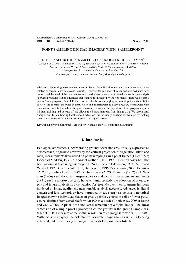
Environmental Monitoring and Assessment (2006) 123: 97–108DOI: 10.1007/s10661-005-9164-7 c© Springer 2006

POINT SAMPLING DIGITAL IMAGERY WITH ‘SAMPLEPOINT’

D. TERRANCE BOOTH1,∗, SAMUEL E. COX1 and ROBERT D. BERRYMAN2

1Rangeland Scientist and Remote Sensing Technician, USDA Agricultural Research Service, HighPlains Grasslands Research Station, 8408 Hildreth Rd, Cheyenne, WY 82009

2Independent Programming Consultant, Boulder, CO(∗author for correspondence, e-mail: Terry.Booth@ars.usda.gov)

Abstract. Measuring percent occurrence of objects from digital images can save time and expenserelative to conventional field measurements. However, the accuracy of image analysis had, until now,not reached the level of the best conventional field measurements. Additionally, most image-analysissoftware programs require advanced user training to successfully analyze images. Here we present anew software program, ‘SamplePoint,’ that provides the user a single-pixel sample point and the abilityto view and identify the pixel context. We found SamplePoint to allow accuracy comparable withthe most accurate field-methods for ground-cover measurements. Expert use of the program requiresminimal training and its ease of use allows rapid measurements from image data. We recommendSamplePoint for calibrating the threshold-detection level of image-analysis software or for makingdirect measurements of percent occurrence from digital images.

Keywords: cover measurement, ground cover, image analysis, point frame, sampling

1. Introduction

Ecological assessments incorporating ground-cover (the area, usually expressed asa percentage, of ground covered by the vertical projection of vegetation, litter, androck) measurements have relied on point sampling using point frames (Levy, 1927;Levy and Madden, 1933) or transect methods (ITT, 1996). Ground cover has alsobeen measured from images (Cooper, 1924; Pierce and Eddleman, 1973; Ratliff andWestfall, 1973; Owens et al., 1985; Harris et al., 1996; Bennet et al., 2000; Everitt etal., 2001; Louhaichi et al., 2001; Richardson et al., 2001). Avery (1962) and Clav-eran (1966) used dot-grid transparencies to make cover measurements and Wells(1971) used a microscope grid; however, until recently the adoption of photogra-phy and image analysis as a convention for ground-cover measurements has beenhindered by image quality and questionable analysis accuracy. Advances in digitalcamera and lens technology have improved image sharpness so that 1-mm/pixelimages showing individual blades of grass, pebbles, cracks in soil or flower petalscan be obtained from aerial platforms at 100-m altitude (Booth et al., 2005c; Boothand Cox, 2006). (A pixel is the smallest discreet unit of a digital image. The lineardimension of a single pixel’s projection on the ground is the ground sample dis-tance (GSD), a measure of the spatial resolution of an image (Comer et al., 1998)).With this new imagery, the potential for accurate image analysis is closer to beingachieved, but the accuracy of analysis methods has posed an obstacle.

98 D. T. BOOTH ET AL.

The image-analysis methods of Avery, Claveran, and Wells (op. cit.) wereadapted to digital images by using a semi-transparent digital-grid overlay(DGO)(Photo Paint v 8.2, Corel Corp., Ottowa, Canada1) on a computer moni-tor (Booth et al., 2005a, b, d). Recent work by Booth et al. (2005d) shows thatwhile field methods such as the Point Intercept, Steel Point Frame and even Oc-ular Estimation had 97–99% accuracy when tested using 2-dimensional modelswith known ground-cover populations, the DGO had an accuracy of only 92%.Further, VegMeasure, an automated image-analysis software program, had accu-racy of only 70% when the algorithm-detection threshold was calibrated with theDGO (Booth et al., 2005b, d).

The contact area of a point-sampling device is recognized as influencing accu-racy (Cook and Stubendieck, 1986; Booth et al., 2005d), and appears to explainwhy the DGO, with a GSD-contact point of 8 mm2, had lower accuracy than almostall other methods, even though the point-sampling density was the same amongall methods (100 points/m2)(Booth et al., 2005d). A more accurate image analysistool was needed.

The measurement of ground cover from images has several potential advantages,including acceleration of field work, increased flexibility, repeatability, and con-venience in the time and place actual measurements are made. Our objective wasto improve image point-sampling accuracy by developing an ‘image point frame’with a reduced contact-point area and increased user-friendliness and efficiency.The expected benefit was confidence in the method so that the advantages notedabove could be realized and applied in environmental monitoring. We named thenew software ‘SamplePoint’ and here we describe the software and tests of itsaccuracy, precision, and utility.

2. SamplePoint Software

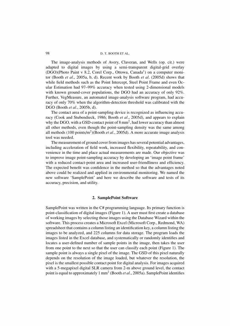
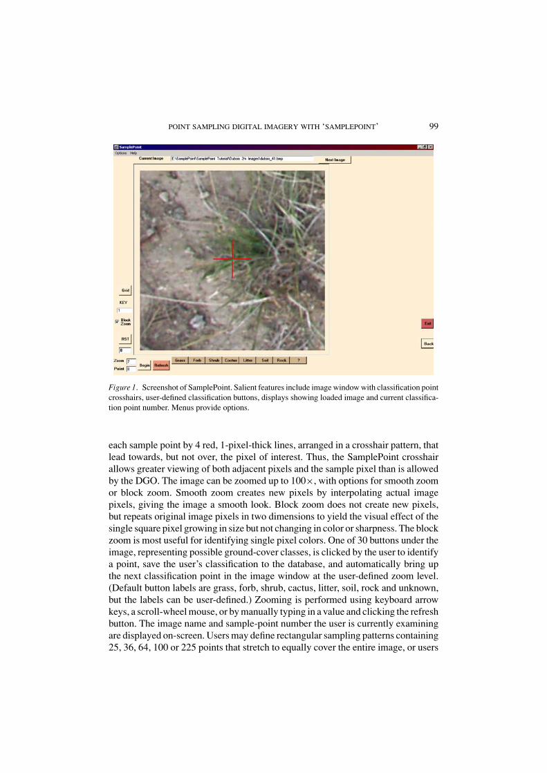
SamplePoint was written in the C# programming language. Its primary function ispoint-classification of digital images (Figure 1). A user must first create a databaseof working images by selecting those images using the Database Wizard within thesoftware. This process creates a Microsoft Excel (Microsoft Corp., Redmond, WA)spreadsheet that contains a column listing an identification key, a column listing theimages to be analyzed, and 225 columns for data storage. The program loads theimages listed in the Excel database, and systematically or randomly identifies andlocates a user-defined number of sample points in the image, then takes the userfrom one point to the next so that the user can classify each point (Figure 1). Thesample point is always a single pixel of the image. The GSD of this pixel naturallydepends on the resolution of the image loaded, but whatever the resolution, thepixel is the smallest possible contact point for digital analysis. For images acquiredwith a 5-megapixel digital SLR camera from 2-m above ground level, the contactpoint is equal to approximately 1 mm2 (Booth et al., 2005a). SamplePoint identifies

POINT SAMPLING DIGITAL IMAGERY WITH ‘SAMPLEPOINT’ 99

Figure 1. Screenshot of SamplePoint. Salient features include image window with classification pointcrosshairs, user-defined classification buttons, displays showing loaded image and current classifica-tion point number. Menus provide options.

each sample point by 4 red, 1-pixel-thick lines, arranged in a crosshair pattern, thatlead towards, but not over, the pixel of interest. Thus, the SamplePoint crosshairallows greater viewing of both adjacent pixels and the sample pixel than is allowedby the DGO. The image can be zoomed up to 100×, with options for smooth zoomor block zoom. Smooth zoom creates new pixels by interpolating actual imagepixels, giving the image a smooth look. Block zoom does not create new pixels,but repeats original image pixels in two dimensions to yield the visual effect of thesingle square pixel growing in size but not changing in color or sharpness. The blockzoom is most useful for identifying single pixel colors. One of 30 buttons under theimage, representing possible ground-cover classes, is clicked by the user to identifya point, save the user’s classification to the database, and automatically bring upthe next classification point in the image window at the user-defined zoom level.(Default button labels are grass, forb, shrub, cactus, litter, soil, rock and unknown,but the labels can be user-defined.) Zooming is performed using keyboard arrowkeys, a scroll-wheel mouse, or by manually typing in a value and clicking the refreshbutton. The image name and sample-point number the user is currently examiningare displayed on-screen. Users may define rectangular sampling patterns containing25, 36, 64, 100 or 225 points that stretch to equally cover the entire image, or users

100 D. T. BOOTH ET AL.

may elect to have from 1 to 200 points randomly placed across the image, butno closer than 30 pixels to the edge. Users can begin point classification at point1, or specify the starting point, and likewise can begin with the first image ofthe database or specify an image. Classification data, as well as the red, green,blue (RGB) values (spectral components) for each classified point, are saved to thedatabase. A summary text file can be generated that lists the total cover for each classfor each image. A summary text file listing the RGB values associated with eachpixel classification can also be generated to determine the spectral distinctivenessof particular classes.

3. A Standard for Comparison: Benchmark Images and Poster Photos

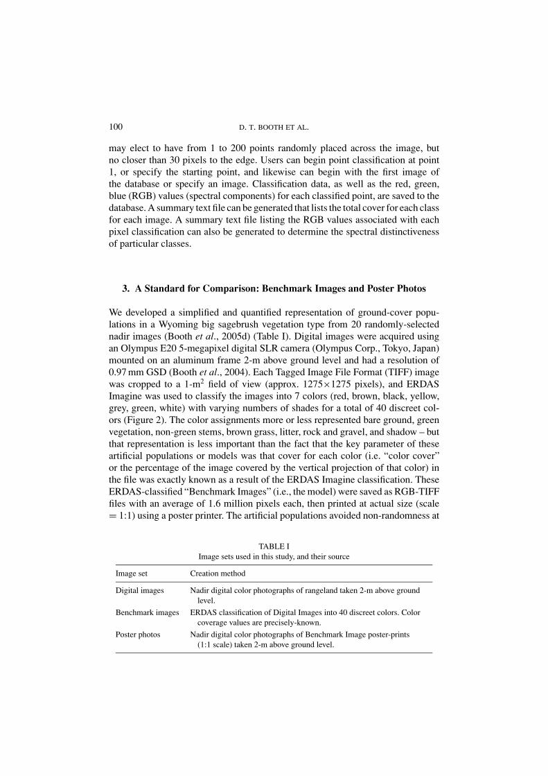
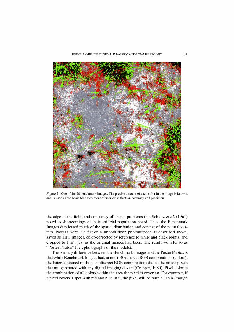
We developed a simplified and quantified representation of ground-cover popu-lations in a Wyoming big sagebrush vegetation type from 20 randomly-selectednadir images (Booth et al., 2005d) (Table I). Digital images were acquired usingan Olympus E20 5-megapixel digital SLR camera (Olympus Corp., Tokyo, Japan)mounted on an aluminum frame 2-m above ground level and had a resolution of0.97 mm GSD (Booth et al., 2004). Each Tagged Image File Format (TIFF) imagewas cropped to a 1-m2 field of view (approx. 1275×1275 pixels), and ERDASImagine was used to classify the images into 7 colors (red, brown, black, yellow,grey, green, white) with varying numbers of shades for a total of 40 discreet col-ors (Figure 2). The color assignments more or less represented bare ground, greenvegetation, non-green stems, brown grass, litter, rock and gravel, and shadow – butthat representation is less important than the fact that the key parameter of theseartificial populations or models was that cover for each color (i.e. “color cover”or the percentage of the image covered by the vertical projection of that color) inthe file was exactly known as a result of the ERDAS Imagine classification. TheseERDAS-classified “Benchmark Images” (i.e., the model) were saved as RGB-TIFFfiles with an average of 1.6 million pixels each, then printed at actual size (scale= 1:1) using a poster printer. The artificial populations avoided non-randomness at

TABLE IImage sets used in this study, and their source

Image set Creation method

Digital images Nadir digital color photographs of rangeland taken 2-m above groundlevel.

Benchmark images ERDAS classification of Digital Images into 40 discreet colors. Colorcoverage values are precisely-known.

Poster photos Nadir digital color photographs of Benchmark Image poster-prints(1:1 scale) taken 2-m above ground level.

POINT SAMPLING DIGITAL IMAGERY WITH ‘SAMPLEPOINT’ 101

Figure 2. One of the 20 benchmark images. The precise amount of each color in the image is known,and is used as the basis for assessment of user-classification accuracy and precision.

the edge of the field, and constancy of shape, problems that Schultz et al. (1961)noted as shortcomings of their artificial population board. Thus, the BenchmarkImages duplicated much of the spatial distribution and context of the natural sys-tem. Posters were laid flat on a smooth floor, photographed as described above,saved as TIFF images, color-corrected by reference to white and black points, andcropped to 1 m2, just as the original images had been. The result we refer to as“Poster Photos” (i.e., photographs of the models).

The primary difference between the Benchmark Images and the Poster Photos isthat while Benchmark Images had, at most, 40 discreet RGB combinations (colors),the latter contained millions of discreet RGB combinations due to the mixed pixelsthat are generated with any digital imaging device (Crapper, 1980). Pixel color isthe combination of all colors within the area the pixel is covering. For example, ifa pixel covers a spot with red and blue in it, the pixel will be purple. Thus, though

102 D. T. BOOTH ET AL.

the posters printed from the Benchmark Images had only 40 colors, each time animage pixel covered an area that had two or more colors (an edge) the pixel colorwas a new, non-standard color born from that combination. Millions such colorswere generated in the Poster Photos that were not present in the Benchmark Images.These mixed-pixels represent an obstacle to accurate image analysis.

In summary, the images for study included a known-population digital image(Benchmark Image) that simulated and simplified (modeled) the pattern and distri-bution of real-world rangeland vegetation, plus a photograph of the model (PosterPhoto). Readers should not interpret either the Benchmark Images or Poster Photosas being intended to represent the actual ground-cover values of the photographedsites. We believe this method for modeling plant communities has application to anysituation or plant community where there is a need to model the spatial distributionand context of the natural system while avoiding non-randomness and constancyof shape.

4. Accuracy Testing

Using the 20 Benchmark Images and 20 Poster Photos, three users with vegetation-sampling backgrounds, ages 27–44, used SamplePoint to measure color cover foreach 20-image data set three times (six 20-image data sets for each user). Boothet al. (2005a) have shown that users older than 50 years measure more bare groundfrom digital images than users under 50. The order of image set classification wasrandomly chosen, with no more than a single 20-image set classified in one day.Correlation coefficients were generated by three separate analyses of measured-to-known values for all seven colors: 1) to measure the repeatability of single users wecompared the variation of three measured-to-known correlation coefficients amongthe three replicates for each user (n = 7 colors × 20 images = 140 observations),2) to measure repeatability among users we compared three replicates × 7 colors ×20 images (n = 420 observations) and 3) to establish the efficacy of SamplePointsoftware we used all observations (n = 3 users × 3 replicates × 7 colors × 20images = 1260 observations). From each user’s data, we randomly selected datasets from Benchmark and PosterPhoto images for regression analysis to knowncolor-cover values of the original Benchmark Images. Coefficients of variationwere generated to measure relative precision across users. A comparison of knownversus classified colors for 2000 points/image facilitated evaluation of classificationconsistency by a single user over time and among different users.

DGO classification of Poster Photos from previous work (Booth et al., 2005d)was used to compare the performance of SamplePoint using a Poster Photo (mixed-pixel image). Additionally, Benchmark images were classified using DGO to pro-vide a direct comparison to SamplePoint classification of Benchmark Images.

To control for gross color differences among monitors, white point was set to6500 K. All users were provided with a color palette showing the colors used for the

POINT SAMPLING DIGITAL IMAGERY WITH ‘SAMPLEPOINT’ 103

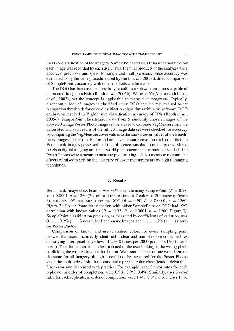
ERDAS classification of the imagery. SamplePoint and DGO classification time foreach image was recorded by each user. Thus, the final products of the analyses wereaccuracy, precision, and speed for single and multiple users. Since accuracy wasevaluated using the same procedure used by Booth et al. (2005d), direct comparisonof SamplePoint’s accuracy with other methods can be made.

The DGO has been used successfully to calibrate software programs capable ofautomated image analysis (Booth et al., 2005b). We used VegMeasure (Johnsonet al., 2003), but the concept is applicable to many such programs. Typically,a random subset of images is classified using DGO and the results used to setrecognition thresholds for color-classification algorithms within the software. DGOcalibration resulted in VegMeasure classification accuracy of 70% (Booth et al.,2005d). SamplePoint classification data from 5 randomly-chosen images of theabove 20-image Poster-Photo image set were used to calibrate VegMeasure, and theautomated analysis results of the full 20-image data set were checked for accuracyby comparing the VegMeasure cover values to the known cover values of the Bench-mark Images. The Poster Photos did not have the same cover for each color that theBenchmark Images possessed, but the difference was due to mixed pixels. Mixedpixels in digital imaging are a real-world phenomenon that cannot be avoided. ThePoster Photos were a means to measure pixel-mixing – thus a means to measure theeffects of mixed pixels on the accuracy of cover measurements by digital imagingtechniques.

5. Results

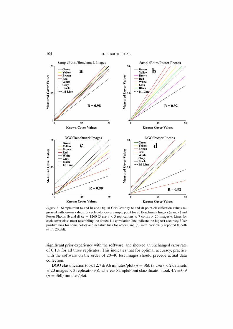
Benchmark Image classification was 98% accurate using SamplePoint (R = 0.98,P < 0.0001, n = 1260 (3 users × 3 replications × 7 colors × 20 images); Figure3), but only 90% accurate using the DGO (R = 0.90, P < 0.0001, n = 1260;Figure 3). Poster Photo classification with either SamplePoint or DGO had 92%correlation with known values (R = 0.92, P < 0.0001, n = 1260; Figure 3).SamplePoint classification precision, as measured by coefficients of variation, was0.11 ± 0.2% (n = 3 users) for Benchmark Images and 1.1 ± 1.2% (n = 3 users)for Poster Photos.

Comparison of known and user-classified colors for every sampling pointshowed that users incorrectly identified a clear and unmistakable color, such asclassifying a red pixel as yellow, 11.2 ± 8 times per 2000 points (<1%) (n = 3users). This ‘human error’ can be attributed to the user looking at the wrong pixel,or clicking the wrong classification button. We assume this error rate would remainthe same for all imagery, though it could not be measured for the Poster Photossince the multitude of similar colors make precise color classification debatable.User error rate decreased with practice. For example, user 2 error rates for eachreplicate, in order of completion, were 0.9%, 0.9%, 0.4%. Similarly, user 3 errorrates for each replicate, in order of completion, were 1.4%, 0.8%, 0.6%. User 1 had

104 D. T. BOOTH ET AL.

Figure 3. SamplePoint (a and b) and Digital Grid Overlay (c and d) point-classification values re-gressed with known values for each color-cover sample point for 20 Benchmark Images (a and c) andPoster Photos (b and d) (n = 1260 (3 users × 3 replications × 7 colors × 20 images)). Lines foreach cover class most resembling the dotted 1:1 correlation line indicate the highest accuracy. Userpositive bias for some colors and negative bias for others, and (c) were previously reported (Boothet al., 2005d).

significant prior experience with the software, and showed an unchanged error rateof 0.1% for all three replicates. This indicates that for optimal accuracy, practicewith the software on the order of 20–40 test images should precede actual datacollection.

DGO classification took 12.7±9.6 minutes/plot (n = 360 (3 users × 2 data sets× 20 images × 3 replications)), whereas SamplePoint classification took 4.7 ± 0.9(n = 360) minutes/plot.

POINT SAMPLING DIGITAL IMAGERY WITH ‘SAMPLEPOINT’ 105

VegMeasure classification accuracy improved from 70% when calibrated withDGO (R = 0.70 ± 0.06, P < 0.0001, n = 420 (3 users × 7 colors × 20 images))(Booth et al., 2005d) to 82% (R = 0.82 ± .02, P < 0.0001, n = 420) whencalibrated with Sample Point.

6. Discussion

For Benchmark Image classification, the higher accuracy of SamplePoint relativeto the DGO is attributed to the 1-pixel sample point. Black was noticeably under-counted in all classifications, suggesting that perhaps users subconsciously chose anearby color when confronted with the void of black (Figure 3). Red was most of-ten overcounted, perhaps because red was the most noticeable color in the imagery.This color bias was previously detected and reported (Booth et al., 2005d) and sug-gests that brightly colored objects (vegetation) are likely to be overcounted at theexpense of drab-colored objects (soil or rock). On the other hand, color perceptionin humans is likely not based on a single factor, but rather it is influenced by multipleperceptual factors (such as object shape) that create small systematic distortions inperceived color hues (Abramov and Gordan, 1994; Goldstone, 1995). Complicatingmatters even more, Brown and MacLeod (1997) concluded that color perceptionwas influenced by surrounding color hue and distribution. We did not measurethe effect of color spatial distribution or relations in the experiment, but researchshows that these play some role in classification. Teasing these factors out wouldbe interesting, but not critical to promoting accurate rangeland cover-measurementstrategies.

The 98% accuracy of SamplePoint classification of Benchmark Images equaledthat of the Point Intercept method (R = 0.98, n = 420 (3 users × 7 colors× 20 images)), and was only slightly lower than the Steel Point Frame method(R = 0.99, n = 420) (Booth et al., 2005d). For routine classification, SamplePointprovides potential accuracy comparable with these conventional field methods ina 2-dimensional setting. We speculate that in the complexity of a 3-dimensionalenvironment, image analysis by SamplePoint would be more accurate than con-ventional methods. The 99 and 98% accuracy rates of the Steel Point Frame andthe Point Intercept methods represent accuracy possible with our 2-dimensionalmodels and not what should be expected for measurements made in 3-dimensional‘real-world’ environments. We are unable to quantify sources of error for the PointIntercept and Steel Point Frame under real-world conditions beyond the commentsof Walker (1980) and others (Friedel and Shaw, 1987; NRC, 1994; Donahue, 1999)but can do so for digital images. There are two primary sources of error inherent ina captured digital image. These are error due to parallax or “camera view” (Bennettet al., 2000), and error due to mixed pixels where different reflected spectra mix andform colors not true to the reflecting entities. Both factors influence the correlationof SamplePoint measurements with the Benchmark and the Poster Photo images.

106 D. T. BOOTH ET AL.

The 92% correlation between known and SamplePoint measurements of Poster-Photo images is thus a good approximation of the accuracy to be expected underoperational conditions using photographs of comparable quality and resolution.We question whether conventional measurements in 3-dimensional environmentseven approach 90% accuracy. Additionally, the increase in sample numbers thatis possible when using a camera, as described above, results in greater statisticalpower relative to using the Steel Point Frame or other conventional field-samplingmethods (Brady et al., 1995; Sundt, 2002).

When used as a calibration tool, SamplePoint also delivers benefits relative tothe DGO, as automated classification accuracy with VegMeasure improved 12%.Combined with the ease of use, time savings and elimination of potential dataentry errors, SamplePoint shows itself to be a very useful tool for image pointclassification, both as a stand-alone tool and as a calibration method for automated-analyses.

Acknowledgments

The research was funded in part by the US Department of Interior,Wyoming State Office of the Bureau of Land Management. Pam Free-man and Adele Legerski provided technical assistance. SamplePoint softwarecan be obtained from the USDA-ARS at: http://www.ars.usda.gov/services/software/download.htm?softwareid=109.

Note

1. Throughout this paper mention of products and proprietary names is for information only and doesnot constitute an endorsement by the authors, USDA, or USDI.

References

Abramov, I. and Gordon, J.: 1994, ‘Color appearance: On seeing red- or yellow, or green, or blue’,Annual Review of Psychology 45, 451–485.

Avery, T. E.: 1962, Interpretation of Aerial photographs, Burgess, Minneapolis, MN, 192 p.Bennett, L. T., Judd, T. S. and Adams, M. A.: 2000, ‘Close-range vertical photography for measuring

cover changes in perennial grasslands’, Journal of Range Management 53, 634–641.Booth, D. T., Cox, S. E., Louhaichi, M. and Johnson, D. E.: 2004, ‘Lightweight camera stand for

close-to-earth remote sensing’, Journal of Range Management 57, 675–678.Booth, D. T., Cox, S. E., Fifield, C., Phillips, M. and Williamson, N.: 2005a, ‘Image analysis compared

with other methods for measuring ground cover’, Arid Land Research and Management 19, 91–100.

Booth, D. T., Cox, S. E. and Johnson, D. E.: 2005b, ‘Detection-threshold calibration and other factorsinfluencing digital measurements of bare ground’, Rangeland Ecology and Management 58, 598–604.

POINT SAMPLING DIGITAL IMAGERY WITH ‘SAMPLEPOINT’ 107

Booth, D. T., Cox, S. E. and Berryman, R. D.: 2005c, ‘Precision measurements from very large scaleaerial digital imagery’, Environmental Monitoring and Assessment 112, 293–307.

Booth, D. T., Cox, S. E., Meikle, T. W. and Fitzgerald, C.: 2005d, ‘The accuracy of ground covermeasurements’, Rangeland Ecology and Management 59, 179–188.

Booth, D. T., Cox, S. E.: 2006, ‘Very-large scale aerial photography for rangeland monitoring’,Geocarto International 21(3), 27–34.

Brady, W. W., Mitchel, J. E., Bonham, C. D. and Cook, J. W.: 1995, ‘Assessing the power of thepoint-line transect to monitor changes in plant basal cover’, Journal of Range Management 48,187–190.

Brown, R. O. and MacLeod, D. I.: 1997, ‘Color appearance depends on the variance of surroundcolors’, Curr Biol. 7, 844–849.

Claveran, R. A.: 1966, ‘Two modifications to the vegetation photographic charting method’, Journalof Range Management 19, 371–373.

Cook, C. W. and Stubbendieck, J.: 1986, Range research: Basic Problems and Techniques, Societyfor Range Management, Denver, CO. 317 p.

Cooper, W. S.: 1924, ‘An apparatus for photographic recording of quadrats’, Journal of Ecology 12,317–321.

Comer, R. P., Kinn, G., Light, D. and Mondello, C.: 1998, ‘Talking digital’, Photogrammetric Engi-neering and Remote Sensing 64, 1139–1142.

Crapper, P. F.: 1980, ‘Errors incurred in estimating an area of uniform land cover using landsat’,Photogrammetric Engineering and Remote Sensing 46, 1295–1301.

Donahue, D. L.: 1999, The Western Range Revisited: Removing Livestock from Public Lands toConserve Native Biodiversity. University of Oklahoma Press, Norman, OK. 388 p.

Everitt, J. H., Yang, C., Racher, B. J., Britton C. M. and Davis, M. R.: 2001, ‘Remote sensing ofredberry juniper in the Texas rolling plains’, Journal of Range Management 54, 254–259.

Friedel, M. H. and Shaw, K.: 1987, ‘Evaluation of methods for monitoring sparse patterned vegetationin arid rangelands. I. Herbage’, Journal of Environmental Management 25, 297–308.

Goldstone, R. L.: 1995, ‘Effects of categorization on color perception’, Psychological Science 6,298–304.

Harris, N. R., Sharrow, S. H. and Johnson, D. E.: 1996, ‘Use of low-level remote sensing to understandtree/forage spatial interactions in agroforests’, Geocarto International 11(3), 81–92.

Interagency Technical Team (ITT): 1996, Sampling Vegetation Attributes, Interagency TechnicalReference, Report No. BLM/RS/ST-96/002+1730. Denver, CO: U.S. Department of the Inte-rior, Bureau of Land Management – National Applied Resources Science Center. Available at:http://www.blm.gov/nstc/library/pdf/samplveg.pdf. Accessed 2 Nov. 2005.

Johnson, D. E., Vulfson, M., Louhaichi, M. and Harris, N. R.: 2003, VegMeasure v.1.6 user’s manual,Department of Rangeland Resources, Oregon State University, Corvallis, OR. 51 p.

Levy, E. B.: 1927, ‘Grasslands of New Zealand’, New Zealand Journal of Agriculture 34, 143–164.Levy, E. B. and Madden, E. A.: 1933, ‘The point method of pasture analysis’ New Zealand Journal

of Agriculture 46, 267–269.Louhaichi, M., Borman, M. M. and Johnson, D. E.: 2001, ‘Spatially located platform and aerial

photography for documentation of grazing impacts on wheat’, Geocarto International 16(1),63–68.

National Research Council (NRC): 1994, Rangeland health, National Academy Press, Washington,D.C., 180 p.

Owens, M. K., Gardiner, H. G. and Norton, B. E.: 1985, ‘A photographic technique for repeatedmapping of rangeland plant populations in permanent plots’, Journal of Range Management 38,231–232.

Pierce, W. R. and Eddleman, L. E.: 1973, ‘A test of stereophotographic sampling in grasslands’Journal of Range Management 26, 148–150.

108 D. T. BOOTH ET AL.

Ratliff, R. D. and Westfall, S. E.: 1973, ‘A simple stereophotographic technique for analyzing smallplots’, Journal of Range Management 26, 147–150.

Richardson, M. D., Karcher, D. E. and Purcell, L. C.: 2001, ‘Quantifying turfgrass cover using digitalimage analysis’, Crop Science 41, 1884–1888.

Sundt, P.: 2002, ‘The statistical power of rangeland monitoring data’, Rangelands 24(2), 16–20.Schultz, A. M., Gibbens, R. P. and Debano, L.: 1961, ‘Artificial populations for teaching and testing

range techniques’, Journal of Range Management 14, 236–242.Walker, B. H.: 1970, ‘An evaluation of eight methods of botanical analysis on grasslands in Rhodesia’,

Journal of Applied Ecology 7, 403–416.Wells, K. F.: 1971, ‘Measuring vegetation changes on fixed quadrats by vertical ground stereopho-

tography,’ Journal of Range Management 24, 233–236.