Point Registration via Efficient Convex Relaxation

Haggai Maron Nadav Dym Itay Kezurer Shahar Kovalsky Yaron LipmanWeizmann Institute of Science

(a) (d)(c)(b) (e)

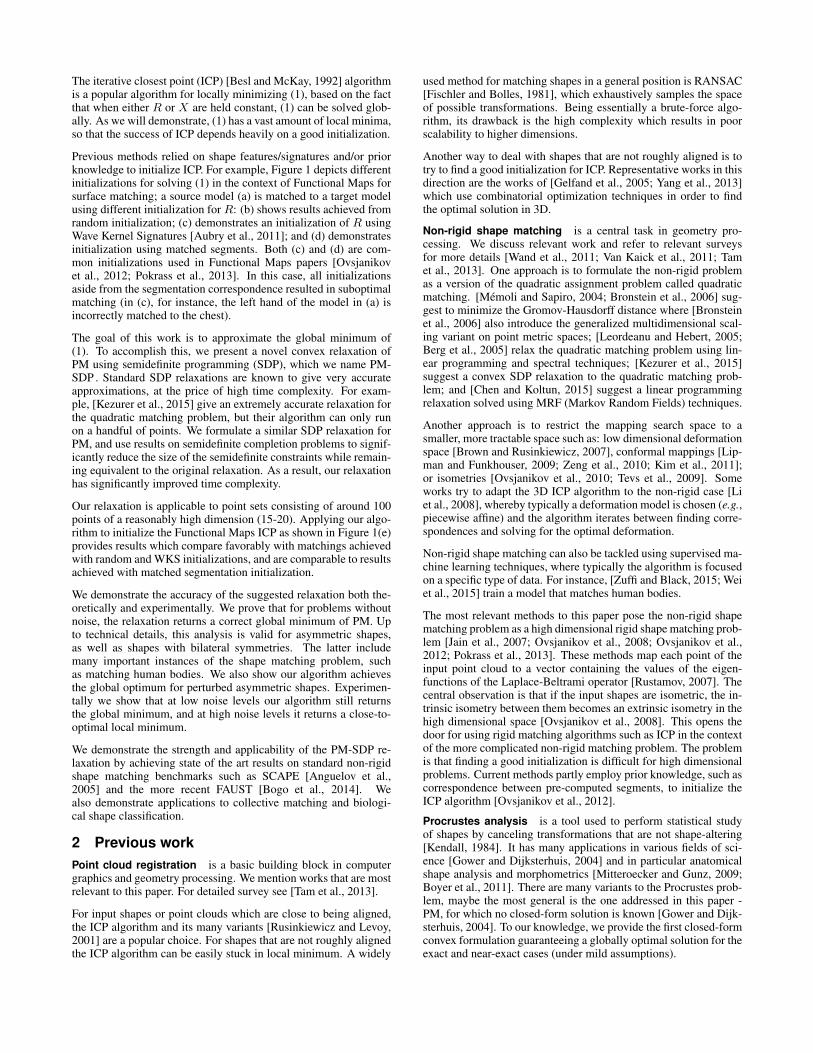
Figure 1: Initializing high-dimensional ICP for non-rigid registration of two human surfaces using different methods: (a) input shape; (b)random initialization; (c) initialization using Wave Kernel Signatures (four examples are shown to its left); (d) initialization with segmentcorrespondence (four examples are shown to its left). The initialization is crucial for good matching; in (e) we show the result of initializationusing PM-SDP which provides comparable result to (d).

Abstract

Point cloud registration is a fundamental task in computer graph-ics, and more specifically, in rigid and non-rigid shape matching.The rigid shape matching problem can be formulated as the prob-lem of simultaneously aligning and labelling two point clouds in 3Dso that they are as similar as possible. We name this problem theProcrustes matching (PM) problem. The non-rigid shape matchingproblem can be formulated as a higher dimensional PM problemusing the functional maps method. High dimensional PM prob-lems are difficult non-convex problems which currently can onlybe solved locally using iterative closest point (ICP) algorithms orsimilar methods. Good initialization is crucial for obtaining a goodsolution.

We introduce a novel and efficient convex SDP (semidefinite pro-gramming) relaxation for the PM problem. The algorithm is guar-anteed to return a correct global solution of the problem whenmatching two isometric shapes which are either asymmetric or bi-laterally symmetric.

We show our algorithm gives state of the art results on popularshape matching datasets. We also show that our algorithm givesstate of the art results for anatomical classification of shapes. Fi-nally we demonstrate the power of our method in aligning shapecollections.

Keywords: Point registration, Shape matching, Convex relaxation

Concepts: •Computing methodologies→ Shape analysis;

Permission to make digital or hard copies of all or part of this work forpersonal or classroom use is granted without fee provided that copies are notmade or distributed for profit or commercial advantage and that copies bearthis notice and the full citation on the first page. Copyrights for componentsof this work owned by others than ACM must be honored. Abstracting withcredit is permitted. To copy otherwise, or republish, to post on servers or toredistribute to lists, requires prior specific permission and/or a fee. Requestpermissions from permissions@acm.org. c© 2016 ACM.SIGGRAPH ’16 Technical Paper,, July 24-28, 2016, Anaheim, CA,ISBN: 978-1-4503-4279-7/16/07

1 Introduction

Registration of point sets is a central problem in computer graphicswith many applications including shape analysis, shape retrieval,statistical shape inference, and shape reconstruction.

Among the different formulations of the point set registrationproblem, the Procrustes matching (PM) formulation is very com-mon: Given two d-dimensional point sets of n points each,P,Q ∈ Rd×n, which are neither aligned nor consistently la-beled, the task is to find a linear isometry (i.e., an orthogo-nal transformation) R ∈ O(d) and a permutation X ∈ Πn

minimizing the distance between the point sets:

d(P,Q) = minX,R‖RP −QX‖2F (1a)

s.t. X ∈ Πn (1b)R ∈ O(d) (1c)

Procrustes matching arises naturally in two and three dimensions(d = 2, 3) for rigid matching problems. Non-rigid matching prob-lems are also often formulated in this way, wherein linear isometriesin higher dimension (d � 3) approximate non-rigid isometries ofthe shapes; this idea is advocated in Functional Maps [Ovsjanikovet al., 2012] where the Laplace-Beltrami eigenfunctions are usedfor the high-dimensional embedding.

The optimization problem (1) is non-convex and globally optimiz-ing it is difficult. In fact, even the subproblem of finding an exact so-lution for PM when such a solution exists (i.e., when d(P,Q) = 0)is difficult. It can be shown that this subproblem can be solvedin polynomial time iff there is a polynomial time algorithm for theexact graph matching problem. The latter is a well researched prob-lem for which no polynomial time algorithm is known.

DOI: http://dx.doi.org/10.1145/2897824.2925913

The iterative closest point (ICP) [Besl and McKay, 1992] algorithmis a popular algorithm for locally minimizing (1), based on the factthat when either R or X are held constant, (1) can be solved glob-ally. As we will demonstrate, (1) has a vast amount of local minima,so that the success of ICP depends heavily on a good initialization.

Previous methods relied on shape features/signatures and/or priorknowledge to initialize ICP. For example, Figure 1 depicts differentinitializations for solving (1) in the context of Functional Maps forsurface matching; a source model (a) is matched to a target modelusing different initialization for R: (b) shows results achieved fromrandom initialization; (c) demonstrates an initialization of R usingWave Kernel Signatures [Aubry et al., 2011]; and (d) demonstratesinitialization using matched segments. Both (c) and (d) are com-mon initializations used in Functional Maps papers [Ovsjanikovet al., 2012; Pokrass et al., 2013]. In this case, all initializationsaside from the segmentation correspondence resulted in suboptimalmatching (in (c), for instance, the left hand of the model in (a) isincorrectly matched to the chest).

The goal of this work is to approximate the global minimum of(1). To accomplish this, we present a novel convex relaxation ofPM using semidefinite programming (SDP), which we name PM-SDP . Standard SDP relaxations are known to give very accurateapproximations, at the price of high time complexity. For exam-ple, [Kezurer et al., 2015] give an extremely accurate relaxation forthe quadratic matching problem, but their algorithm can only runon a handful of points. We formulate a similar SDP relaxation forPM, and use results on semidefinite completion problems to signif-icantly reduce the size of the semidefinite constraints while remain-ing equivalent to the original relaxation. As a result, our relaxationhas significantly improved time complexity.

Our relaxation is applicable to point sets consisting of around 100points of a reasonably high dimension (15-20). Applying our algo-rithm to initialize the Functional Maps ICP as shown in Figure 1(e)provides results which compare favorably with matchings achievedwith random and WKS initializations, and are comparable to resultsachieved with matched segmentation initialization.

We demonstrate the accuracy of the suggested relaxation both the-oretically and experimentally. We prove that for problems withoutnoise, the relaxation returns a correct global minimum of PM. Upto technical details, this analysis is valid for asymmetric shapes,as well as shapes with bilateral symmetries. The latter includemany important instances of the shape matching problem, suchas matching human bodies. We also show our algorithm achievesthe global optimum for perturbed asymmetric shapes. Experimen-tally we show that at low noise levels our algorithm still returnsthe global minimum, and at high noise levels it returns a close-to-optimal local minimum.

We demonstrate the strength and applicability of the PM-SDP re-laxation by achieving state of the art results on standard non-rigidshape matching benchmarks such as SCAPE [Anguelov et al.,2005] and the more recent FAUST [Bogo et al., 2014]. Wealso demonstrate applications to collective matching and biologi-cal shape classification.

2 Previous workPoint cloud registration is a basic building block in computergraphics and geometry processing. We mention works that are mostrelevant to this paper. For detailed survey see [Tam et al., 2013].

For input shapes or point clouds which are close to being aligned,the ICP algorithm and its many variants [Rusinkiewicz and Levoy,2001] are a popular choice. For shapes that are not roughly alignedthe ICP algorithm can be easily stuck in local minimum. A widely

used method for matching shapes in a general position is RANSAC[Fischler and Bolles, 1981], which exhaustively samples the spaceof possible transformations. Being essentially a brute-force algo-rithm, its drawback is the high complexity which results in poorscalability to higher dimensions.

Another way to deal with shapes that are not roughly aligned is totry to find a good initialization for ICP. Representative works in thisdirection are the works of [Gelfand et al., 2005; Yang et al., 2013]which use combinatorial optimization techniques in order to findthe optimal solution in 3D.

Non-rigid shape matching is a central task in geometry pro-cessing. We discuss relevant work and refer to relevant surveysfor more details [Wand et al., 2011; Van Kaick et al., 2011; Tamet al., 2013]. One approach is to formulate the non-rigid problemas a version of the quadratic assignment problem called quadraticmatching. [Memoli and Sapiro, 2004; Bronstein et al., 2006] sug-gest to minimize the Gromov-Hausdorff distance where [Bronsteinet al., 2006] also introduce the generalized multidimensional scal-ing variant on point metric spaces; [Leordeanu and Hebert, 2005;Berg et al., 2005] relax the quadratic matching problem using lin-ear programming and spectral techniques; [Kezurer et al., 2015]suggest a convex SDP relaxation to the quadratic matching prob-lem; and [Chen and Koltun, 2015] suggest a linear programmingrelaxation solved using MRF (Markov Random Fields) techniques.

Another approach is to restrict the mapping search space to asmaller, more tractable space such as: low dimensional deformationspace [Brown and Rusinkiewicz, 2007], conformal mappings [Lip-man and Funkhouser, 2009; Zeng et al., 2010; Kim et al., 2011];or isometries [Ovsjanikov et al., 2010; Tevs et al., 2009]. Someworks try to adapt the 3D ICP algorithm to the non-rigid case [Liet al., 2008], whereby typically a deformation model is chosen (e.g.,piecewise affine) and the algorithm iterates between finding corre-spondences and solving for the optimal deformation.

Non-rigid shape matching can also be tackled using supervised ma-chine learning techniques, where typically the algorithm is focusedon a specific type of data. For instance, [Zuffi and Black, 2015; Weiet al., 2015] train a model that matches human bodies.

The most relevant methods to this paper pose the non-rigid shapematching problem as a high dimensional rigid shape matching prob-lem [Jain et al., 2007; Ovsjanikov et al., 2008; Ovsjanikov et al.,2012; Pokrass et al., 2013]. These methods map each point of theinput point cloud to a vector containing the values of the eigen-functions of the Laplace-Beltrami operator [Rustamov, 2007]. Thecentral observation is that if the input shapes are isometric, the in-trinsic isometry between them becomes an extrinsic isometry in thehigh dimensional space [Ovsjanikov et al., 2008]. This opens thedoor for using rigid matching algorithms such as ICP in the contextof the more complicated non-rigid matching problem. The problemis that finding a good initialization is difficult for high dimensionalproblems. Current methods partly employ prior knowledge, such ascorrespondence between pre-computed segments, to initialize theICP algorithm [Ovsjanikov et al., 2012].

Procrustes analysis is a tool used to perform statistical studyof shapes by canceling transformations that are not shape-altering[Kendall, 1984]. It has many applications in various fields of sci-ence [Gower and Dijksterhuis, 2004] and in particular anatomicalshape analysis and morphometrics [Mitteroecker and Gunz, 2009;Boyer et al., 2011]. There are many variants to the Procrustes prob-lem, maybe the most general is the one addressed in this paper -PM, for which no closed-form solution is known [Gower and Dijk-sterhuis, 2004]. To our knowledge, we provide the first closed-formconvex formulation guaranteeing a globally optimal solution for theexact and near-exact cases (under mild assumptions).

Semidefinite relaxation and polynomial optimization. Con-vex relaxations of quadratic optimization problems are often (e.g.,[Poljak et al., 1995; Luo et al., 2010]) preformed by replacingquadratic terms with new variables. All quadratic terms then be-come linear, and a convex semidefinite constraint is added to cou-ple between the original variables and the new variables. A signifi-cant drawback of these relaxations is that they are computationallytractable only for very small polynomial problems. [Fukuda et al.,2000; Waki et al., 2006] show that for problems with certain struc-ture, a positive semidefinite constraint on a large matrix can be re-placed by constraining certain principal submatrices to be positivesemidefinite, resulting in an equivalent problem with significantlyimproved time complexity. In this paper we devise a quadratic for-mulation of PM which has this structure, and as a result obtain arelaxation which is tractable for medium sized problems.

3 Approach and Formulation

We present our convex relaxation of PM. We first discuss the gen-eral quadratic optimization problem and present a novel strategyfor replacing its “standard” time consuming SDP relaxations withan equivalent, but significantly more efficient SDP relaxation. Inthis context, we then instantiate our relaxation for the PM problem.

Full SDP relaxation of quadratic problems. Quadratic opti-mization problems are problems of the form

minx∈RN

f0(x) (2a)

s.t. fs(x) = 0, s = 1, . . . , S (2b)ft(x) ≥ 0, t = S + 1 . . . T (2c)

where fi are quadratic multivariate polynomials.

A typical relaxation procedure includes two steps (see [Luo et al.,2010] for a survey on SDP quadratic relaxations): First, thequadratic polynomials fi are linearized by introducing new vari-ables Yij , 1 ≤ i, j ≤ N , which replace quadratic monomials xixj ,so that fj(x) becomes a linear polynomial in the variables x, Ydenoted L[fj ](x, Y ). This gives an equivalent formulation of (2):

minx,Y

L [f0] (x, Y ) (3a)

s.t. L [fs] (x, Y ) = 0, s = 1 . . . S (3b)L [ft] (x, Y ) ≥ 0, t = S + 1 . . . T (3c)

Y = xxT (3d)

With the exception of constraint (3d), Problem (3) is a convex prob-lem (in fact a linear program). Therefore, the second step in this re-laxation procedure is replacing (3d) with a convex constraint. Theconvex hull of the set defined by (3d) is the set defined by the con-vex constraint Y � xxT , which is equivalent to the semidefiniteconstraint [

1 xT

x Y

]� 0. (4)

A natural relaxation of (3) is therefore given by replacing (3d) with(4). [Zhao et al., 1998] and more recently [Kezurer et al., 2015]used this approach to relax the quadratic matching and quadraticassignment problems. The obtained relaxation is significantly moreaccurate than prevalent relaxations for quadratic matching, but itsscalability is poor; in fact, it cannot handle more than a handful ofpoints to be matched, completely hindering some applications.

Efficient SDP relaxation. The key to a useful and efficient re-laxation of (2) and consequently our problem (1) is to reduce thedimension of the semi-definite constraint (4) which is the main fac-tor determining time efficiency of the semidefinite program.

To obtain a more efficient SDP relaxation, we make the observationthat for some problems not all terms in the matrix xxT appear in thepolynomials fj . This is, for example, the case in the PM problem,as will soon be shown. In such cases, we can find a collection Jof subsets of {1, . . . , N} so that all polynomials fj include onlyexpressions from xJx

TJ , J ∈ J . An equivalent formulation for

(3) can therefore be obtained by replacing (3d) with YJ = xJxTJ ,

for all J ∈ J . In turn, replacing these with the convex constraints[1 xTJxJ YJ

]� 0, J ∈ J (5)

we obtain a convex relaxation for (2). If all subsets J ∈ J satisfy|J | � N , the obtained relaxation is considerably more efficientthan the original (full) relaxation.

There is no unique way to apply this more efficient relaxation; agiven instance of a quadratic optimization problem may have sev-eral different possible decompositions J . Those that use smallsemidefinite constraints will be more efficient, but not necessar-ily as accurate as those using larger semidefinite constraints; thelatter, however, can quickly become intractable for certain prob-lems. Nevertheless, if J is chosen so that it satisfies the chordalitycondition we will soon describe, the obtained relaxation is in factequivalent to the full relaxation.

In general, any solution for the full relaxation also satisfies (5). Forequivalency, we need to ensure that a solution for the efficient re-laxation (5) can always be completed to a solution of the full relax-ation. For that end we need to show there is a solution for the fol-lowing matrix completion problem: We are given entries of xJ , YJsatisfying (5), and we are searching for a completion of Y that sat-isfies (4). Since the objective and linear constraints depend only onthe coordinates which were determined before the completion, thefull solution will also fulfill the linear constraints, and the objectivewill not be affected by the completion.

The condition that allows solving the completionproblem is related to the structure of the known co-ordinates of the matrix. The collection J definesan undirected graph G = (V,E) whose vertices areV = {1, x1, . . . , xN}. Two distinct vertices are con-nected by an edge iff they both appear in one of thematrices (5) defined by some J ∈ J . A graph G ischordal if every (simple) cycle with more than threevertices contains a chord, i.e., an edge between twonon-adjacent members of the cycle. For example the graph in thetop of the inset has a cycle which does not contain a chord and thusis not a chordal graph. The bottom graph is chordal.

If G is chordal, the following theorem from [Grone et al., 1984]guarantees that the matrix completion problem has a solution, andtherefore that the two relaxations are equivalent:Theorem 1. If G is chordal, and (xJ , YJ)J∈J satisfy (5), then themissing coordinates of Y can be chosen so that the full semidefiniteconstraint (4) holds.

PM-SDP Formulation. We now return to the PM problem andinstantiate the strategy presented above. First, we note that PM canbe formulated as the following quadratic problem:

minX,R‖RP −QX‖2F (6a)

X1 = 1, 1TX = 1T (6b)

XjXTj = diag(Xj), j = 1 . . . n (6c)

RRT = RTR = I (6d)

where we denote by 1 ∈ Rn×1 the all-ones vector, by Xj the j-thcolumn ofX , and by diag(Xj) the diagonal matrix whose diagonalentries are Xj .

To see this is indeed an equivalent formulation of PM, note that if(R,X) is a feasible solution of (6), then R is orthogonal by defini-tion. The constraint (6c) implies that X2

ij = Xij for all i, j, so thatall elements of X are in {0, 1}. By (6b) the rows and columns ofX sum to one, which implies that X is a permutation matrix.

In the other direction, note that if (R,X) ∈ O(d) × Πn, thensince each column of X has only one non-zero element, XjXT

j isdiagonal. Since all elements of X are in {0, 1}, X2

ij = Xij for alli, j so that (6c) holds. It is straightforward to check that (6b),(6d)hold as well.

All polynomials in (6) are quadratic in the entries of R and X .The full SDP relaxation for quadratic problems described abovecan then be applied; this will result in a vector x, consisting of theelements of R and X , of dimension d2 + n2; the SDP constraintwill be of size (d2 + n2 + 1)× (d2 + n2 + 1).

We obtain an equivalent, more efficient, relaxation by utilizing theefficient SDP relaxation approach; the key observation here is thatall the quadratic polynomials participating in the formulation (6) ofthe PM problem can be expressed using linear polynomials in theentries of XjXT

j , Xj [R]T , and [R] [R]T , where [R] ∈ Rd2×1 is

the column stack of the matrix R and j = 1 . . . n. We thereforeintroduce new matrix variables Zj , constrained to satisfy

Zj =

[Xj[R]

] [Xj[R]

]T, j = 1 . . . n (7)

Let us next see how the objective and constraints of Problem (6) arelinear in the variables X,R,Zj . First, the objective of (6) can berewritten as

‖RP −QX‖2F =∑j

‖RPj −QXj‖22 =∑j

tr (WjZj)+const

for some constant matrices Wj since ‖RPj −QXj‖22 is linear inthe entries of Zj . Denoting

Zj =

[Aj BTjBj C

], Aj ∈ Rn×n, C ∈ Rd

2×d2 , Bj ∈ Rd2×n (8)

the constraint (6c) can be rewritten as Aj = diag(Xj). Finally, theconstraints (6d) are affine functions of C and can be rewritten as

tr(H`C) + b` = 0, ` = 1 . . . 2d2

for some constant matrices H`. Replacing the non-convex equalityconstraint of (7) with convex semidefinite constraints of type (4),we obtain our relaxation for the PM problem, PM-SDP:

minZj ,X,R

∑j

tr (WjZj) (9a)

X1 = 1, 1TX = 1T (9b)Aj = diag(Xj), j = 1 . . . n (9c)

tr(H`C) + b` = 0, ` = 1 . . . 2d2 (9d)

Zj �[Xj[R]

] [Xj[R]

]T, j = 1 . . . n (9e)

where Aj and C are defined as in (8).

Figure 2: The graph corresponding to the Procrustes Problem(right, each disk represents a clique) is chordal, that is, has no min-imal cycles of length at-least four. The adjacency matrix is shownon the left.

Chordality of the relaxation. To show that (9) is equivalent tothe full relaxation of the PM problem, we need to show that thegraph G induced by J = {Jj} is chordal, where Jj is the setcontaining the variables [R] and Xj . The adjacency matrix of Gfor this case is illustrated in Figure 2 (left) where each gray squarerepresents a full block of ones; on the right, we illustrate the corre-sponding graph G where each disk represents a clique which corre-sponds to a diagonal block in the adjacency matrix. To show G ischordal it is enough to show every cycle of length at-least 4 has achord: Indeed, if a cycle is completely contained in one of the setsJj (represented as triangles in Figure 2, right) then any two verticesare connected by an edge; otherwise there are two non consecutivevisits to vertices in the 1, [R] cliques (top disks), and these verticesare connected by an edge.

Dimension and complexity. We note that (9e) includes nsemidefinite constraints involving N × N matrices, where N =d2 + n + 1, as opposed to the full relaxation which in this casewould involve a square matrix with N = d2 + n2 + 1. When thenumber of points in the sets n is significantly larger than the di-mension d of the space the point reside in (i.e., n � d), whichis often the case in point registration problems, PM-SDP will besignificantly more efficient than the full SDP relaxation.

Relaxation properties. The PM-SDP relaxation has the follow-ing natural theoretical properties:

1. Rotation and relabeling invariance: Rotating or relabeling theinput shapes will not affect the solution provided by the relax-ation. More precisely, if P is replaced with a point cloud P ob-tained from P by relabeling and applying an orthogonal trans-formation, then the objective of PM-SDP remains unchanged,and X,R transform accordingly.

2. Lower bound: Since PM-SDP is a relaxation its optimal objec-tive is less or equal to the PM optimal objective. We denote theobjective of PM-SDP by d.

3. Positivity: The objective of PM-SDP is always non-negative.This is natural since this is the case for the objective of PM .

4. Convex-hull of R,X: The R,X coordinates of a feasible solu-tion for PM-SDP are in the convex hull of O(d)×Πn.

The proof of the these properties as well as the theorems presentedbelow are given in [Dym and Lipman, 2016].

Exact recovery refers to the problem of finding R,X ∈ O(d)×Πn which solve the equation RP = QX , when such solutionsexists, i.e., when d(P,Q) = 0. We call such solutions exact solu-tions. From the computational perspective, exact recovery for PM is

equivalent to exact graph matching. The latter is a well-researchedproblem, not known to be polynomial. Accordingly, proving exactrecovery in full generality is not likely. However, under the assump-tion that the covariance d×dmatrix PPT of the point cloud P hasa simple spectrum, and an additional weak assumption, we are ableto prove exact recovery. This too is analogous to the graph match-ing problem where finding exact solutions for graphs with simplespectrum affinity matrices is solvable in polynomial time [Babaiet al., 1982].

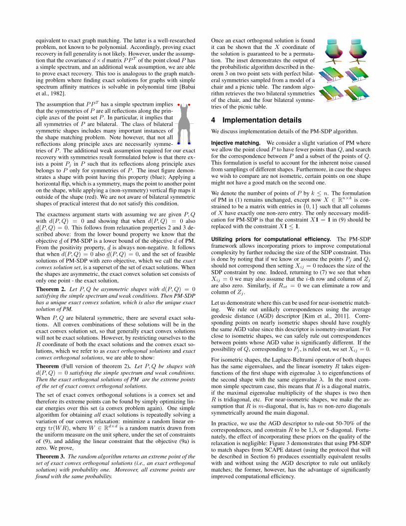
The assumption that PPT has a simple spectrum impliesthat the symmetries of P are all reflections along the prin-ciple axes of the point set P . In particular, it implies thatall symmetries of P are bilateral. The class of bilateralsymmetric shapes includes many important instances ofthe shape matching problem. Note however, that not allreflections along principle axes are necessarily symme-tries of P . The additional weak assumption required for our exactrecovery with symmetries result formulated below is that there ex-ists a point Pj in P such that its reflections along principle axesbelongs to P only for symmetries of P . The inset figure demon-strates a shape with point having this property (blue); Applying ahorizontal flip, which is a symmetry, maps the point to another pointon the shape, while applying a (non-symmetry) vertical flip maps itoutside of the shape (red). We are not aware of bilateral symmetricshapes of practical interest that do not satisfy this condition.

The exactness argument starts with assuming we are given P,Qwith d(P,Q) = 0 and showing that when d(P,Q) = 0 alsod(P,Q) = 0. This follows from relaxation properties 2 and 3 de-scribed above: from the lower bound property we know that theobjective d of PM-SDP is a lower bound of the objective d of PM.From the positivity property, d is always non-negative. It followsthat when d(P,Q) = 0 also d(P,Q) = 0, and the set of feasiblesolutions of PM-SDP with zero objective, which we call the exactconvex solution set, is a superset of the set of exact solutions. Whenthe shapes are asymmetric, the exact convex solution set consists ofonly one point - the exact solution,Theorem 2. Let P,Q be asymmetric shapes with d(P,Q) = 0satisfying the simple spectrum and weak conditions. Then PM-SDPhas a unique exact convex solution, which is also the unique exactsolution of PM.When P,Q are bilateral symmetric, there are several exact solu-tions. All convex combinations of these solutions will be in theexact convex solution set, so that generally exact convex solutionswill not be exact solutions. However, by restricting ourselves to theR coordinate of both the exact solutions and the convex exact so-lutions, which we refer to as exact orthogonal solutions and exactconvex orthogonal solutions, we are able to show:Theorem (Full version of theorem 2). Let P,Q be shapes withd(P,Q) = 0 satisfying the simple spectrum and weak conditions.Then the exact orthogonal solutions of PM are the extreme pointsof the set of exact convex orthogonal solutions.The set of exact convex orthogonal solutions is a convex set andtherefore its extreme points can be found by simply optimizing lin-ear energies over this set (a convex problem again). One simplealgorithm for obtaining all exact solutions is repeatedly solving avariation of our convex relaxation: minimize a random linear en-ergy tr(WR), where W ∈ Rd×d is a random matrix drawn fromthe uniform measure on the unit sphere, under the set of constraintsof (9), and adding the linear constraint that the objective (9a) iszero. We prove,Theorem 3. The random algorithm returns an extreme point of theset of exact convex orthogonal solutions (i.e., an exact orthogonalsolution) with probability one. Moreover, all extreme points arefound with the same probability.

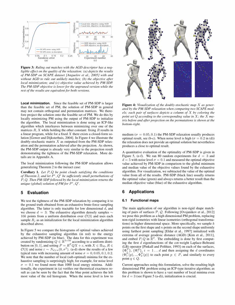
Once an exact orthogonal solution is foundit can be shown that the X coordinate ofthe solution is guaranteed to be a permuta-tion. The inset demonstrates the output ofthe probabilistic algorithm described in the-orem 3 on two point sets with perfect bilat-eral symmetries sampled from a model of achair and a picnic table. The random algo-rithm retrieves the two bilateral symmetriesof the chair, and the four bilateral symme-tries of the picnic table.

4 Implementation detailsWe discuss implementation details of the PM-SDP algorithm.

Injective matching. We consider a slight variation of PM wherewe allow the point cloud P to have fewer points than Q, and searchfor the correspondence between P and a subset of the points of Q.This formulation is useful to account for the inherent noise causedfrom samplings of different shapes. Furthermore, in case the shapeswe wish to compare are not isometric, certain points on one shapemight not have a good match on the second one.

We denote the number of points of P by k ≤ n. The formulationof PM in (1) remains unchanged, except now X ∈ Rn×k is con-strained to be a matrix with entries in {0, 1} such that all columnsof X have exactly one non-zero entry. The only necessary modifi-cation for PM-SDP is that the constraint X1 = 1 in (9) should bereplaced with the constraint X1 ≤ 1.

Utilizing priors for computational efficiency. The PM-SDPframework allows incorporating priors to improve computationalcomplexity by further reducing the size of the SDP constraint. Thisis done by noting that if we know or assume the points Pj and Qishould not correspond then setting Xij = 0 reduces the size of theSDP constraint by one. Indeed, returning to (7) we see that whenXij = 0 we may also assume that the i-th row and column of Zjare also zero. Similarly, if Rst = 0 we can eliminate a row andcolumn of Zj .

Let us demonstrate where this can be used for near-isometric match-ing. We rule out unlikely correspondences using the averagegeodesic distance (AGD) descriptor [Kim et al., 2011]. Corre-sponding points on nearly isometric shapes should have roughlythe same AGD value since this descriptor is isometry-invariant. Forclose to isometric shapes, we can safely rule out correspondencesbetween points whose AGD value is significantly different. If thepossibility ofQi corresponding to Pj , is ruled out, we setXij = 0.

For isometric shapes, the Laplace-Beltrami operator of both shapeshas the same eigenvalues, and the linear isometry R takes eigen-functions of the first shape with eigenvalue λ to eigenfunctions ofthe second shape with the same eigenvalue λ. In the most com-mon simple spectrum case, this means that R is a diagonal matrix,if the maximal eigenvalue multiplicity of the shapes is two thenR is tridiagonal, etc. For near-isometric shapes, we make the as-sumption that R is m-diagonal, that is, has m non-zero diagonalssymmetrically around the main diagonal.

In practice, we use the AGD descriptor to rule-out 50-70% of thecorrespondences, and constrain R to be 1,3, or 5-diagonal. Fortu-nately, the effect of incorporating these priors on the quality of therelaxation is negligible: Figure 3 demonstrates that using PM-SDPto match shapes from SCAPE dataset (using the protocol that willbe described in Section 6) produces essentially equivalent resultswith and without using the AGD descriptor to rule out unlikelymatches; the former, however, has the advantage of significantlyimproved computational efficiency.

0 20 40 60 800

.01

.02Local min. objective: using AGD Local min. objective: no descriptors

0 0.05 0.1 0.15 0.2 0.250

0.2

0.4

0.6

0.8

1

SCAPE errors: using AGD SCAPE errors: no descriptors

0 20 40 60 800

.01

.02SDP objective: using AGD SDP objective: no descriptors

(a)

(b)

(c)

% C

orre

spon

denc

es

Obj

ectiv

eO

bjec

tive

Geodesic error Experiment number

Figure 3: Ruling out matches with the AGD descriptor has a neg-ligible effect on the quality of the relaxation: (a) depicts the resultsof PM-SDP on SCAPE dataset [Anguelov et al., 2005] with andwithout AGD to rule out unlikely matches; (b) the objective afterlocal minimization; and (c) objective value achieved by PM-SDP.The PM-SDP objective is lower for the unpruned version while therest of the results are equivalent for both versions.

Local minimization. Since the feasible set of PM-SDP is largerthan the feasible set of PM, the solution of PM-SDP in generalmay not contain orthogonal and permutation matrices. We there-fore project the solution onto the feasible set of PM. We do this bylocally minimizing PM using the output of PM-SDP to initializethe algorithm. The local minimization is done using an ICP-likealgorithm which interleaves between minimizing over one of thematrices R,X while holding the other constant: fixing R results ina linear program, while for a fixed X there exists a closed-form so-lution [Gower and Dijksterhuis, 2004]. In Figure 4 we illustrate thedoubly-stochastic matrix X as outputted from the PM-SDP relax-ation and the permutation achieved after the projection. As shown,the PM-SDP output is already very similar to the projection resultdemonstrating the tightness of the PM-SDP relaxation. More de-tails are in Appendix A.

The local minimization following the PM-SDP relaxation allowsgeneralizing Theorem 2 to the inexact case:Corollary 1. Let P,Q be point clouds satisfying the conditionsof Theorem 2, and let P ε, Qε be sufficiently small perturbations ofP,Q. Then PM-SDP followed by the local minimization returns theunique (global) solution of PM for P ε, Qε.

5 Evaluation

We test the tightness of the PM-SDP relaxation by comparing it tothe ground truth obtained from an exhaustive brute-force samplingalgorithm. The latter is only tractable for low dimensional d, andwe choose d = 3: The exhaustive algorithm densely samples ∼10k points from a uniform distribution over O(3) and uses eachsample Rj as an initialization for the local minimization algorithmdescribed above.

In Figure 5 we compare the histograms of optimal values achievedby the exhaustive sampling algorithm (in red) to the energyachieved by PM-SDP (in blue). The data for this experiment wascreated by randomizing Q ∈ R3×50 according to a uniform distri-bution on [0, 1], and setting P = RTQX + ε, with X ∈ Π50, R ∈O(3) and noise ε ∼ Nd×n(0, σ2). (a-d) show the results of a fewtypical runs with increasing amount of noise σ = 0, 0.05, 0.1, 0.2.We note that the number of local (sub-optimal) minima for the ex-haustive sampling is surprisingly high; for example, for noise levelσ = 0.1 we found more than 1000 local energy minima. Addi-tionally, the experiment in (a) verifies our theoretical exactness re-sult as can be seen by the fact that the blue point achieves the leftmost value of the red histogram. When the noise level is low to

Figure 4: Visualization of the doubly-stochastic map X as gener-ated by the PM-SDP relaxation when comparing two SCAPE mod-els; each pair of surfaces depicts a column of X by coloring thepoint set Q according to the corresponding value in X; the X ma-trix before and after projection on the permutations is shown at thebottom-right.

medium (σ = 0.05, 0.1) the PM-SDP relaxation usually producesoptimal result, see (b-c). When noise level is high (σ = 0.2 in (d))the relaxation does not provide an optimal solution but neverthelessproduces a close to optimal result.

A quantitative evaluation of the optimality of PM-SDP is given inFigure 5, (e-f). We ran 80 random experiments for d = 3 andd = 5 with noise level σ = 0.1 and measured the optimal objectivevalue achieved by PM-SDP in comparison to the global minimumand median value of the objective values found by the exhaustivealgorithm. For visualization, we subtracted the value of the optimalvalue from all of the results. PM-SDP (black line) usually returnsthe optimal value (green) and always returns a better result than themedian objective value (blue) of the exhaustive algorithm.

6 Applications

6.1 Functional maps

The main application of our algorithm is non-rigid shape match-ing of pairs of surfaces P,Q. Following [Ovsjanikov et al., 2012]we pose this problem as a high dimensional PM problem, replacingnon-rigid isometries with linear isometries (orthogonal transforma-tions) in higher dimensional space. More specifically, we sample kpoints on the first shape and n points on the second shape uniformlyusing farthest point sampling [Eldar et al., 1997] initialized withextrema of average geodesic distance (AGD) [Kim et al., 2011],and embed P,Q in Rd. The embedding is done by first comput-ing the first d eigenfunctions of the cot-weight Laplace-Beltrami(LB) operator [Pinkall and Polthier, 1993] on each of the surfaces,{ΦPi }, {ΦQi }, i = 1 . . . d and then assigning the d coordinates(ΦP1 (p), ..,ΦPd (p)) to each point p ∈ P , and similarly to everypoint q ∈ Q.

Current approaches using this formulation, solve the resulting highdimensional PM problem using an ICP-type iterative algorithm; asthis problem is shown to have a vast number of local minima evenfor d = 3 (see Figure 5 (a-d)), initialization is crucial.

0 20 40 60 80

0

0.2

0.4

0.6

0.8

PM-SDPExhaustive: minimum Exhaustive: median

d =3

0 0.5 1 1.5 2 2.5Objective Value

0

5

10

15%

Exp

erim

ents

Exhaustive algorithm PM-SDP

σ =0

1 1.2 1.4 1.6 1.8Objective Value

0

2

4

6

8

% E

xper

imen

ts

σ =0.1

0.5 1 1.5 2 2.5Objective Value

0

2

4

6

8

10 σ =0.05

1.6 1.8 2 2.2 2.4Objective Value

0

1

2

3

4

5 σ =0.2

0 20 40 60 80

0

0.5

1

1.5 d =5

(a)

(c)

(e)

(b)

(d)

(f)Experiment number Experiment number

Erro

r

Figure 5: PM-SDP tightness evaluation: (a-d) show the histogramsof the objective values achieved by the exhaustive sampling algo-rithm compared to the optimal PM-SDP objective on a few typicalruns. When the noise level is low to medium, our algorithm usu-ally finds the global minimum. On higher noise levels it returnsan objective value close to optimal. (e-f) show illustrations of thedeviation of the optimal PM-SDP objective value from the globaloptimum and the median value computed by the exhaustive algo-rithm when σ = 0.1, d = 3 and d = 5.

Using standard shape signatures or features often does not providea satisfactory initialization (e.g., Figure 1, (b-c)), and previouslythis ICP procedure was initialized with matched segments for suc-cessful results [Ovsjanikov et al., 2012; Pokrass et al., 2013]. Inthe experiments of this subsection we use PM-SDP followed by lo-cal minimization to initialize the ICP of [Ovsjanikov et al., 2012]that uses the entire embedded models. In comparisons to previousworks we used code supplied by the authors with their default pa-rameters.

SCAPE dataset. We evaluated the performance of PM-SDP fornon-rigid isometric matching using the SCAPE dataset [Anguelovet al., 2005]. We used n = 100 sampled points, d = 17 eigen-functions, and injective mapping of k = 50 out of n = 100 . Forbetter efficiency we allowed each point in P to be matched only tothe 30% of the points in Q that have the closest AGD, and selectedm = 5 (5 non-zero diagonals in R). The SDP optimization wasperformed using Mosek [MOSEK, 2015]. We extended our resultsto a full correspondence of all the vertices by solving ICP in dimen-sion d = 30. The average running time for a pair with these settingsis 30-35 minutes on an Intel Xeon E5 CPU. We also tested a fasterversion by taking d = 30 and using diagonal R, that is m = 1; thisgave only slightly inferior results with running time of 2.5 minutesper pair.

0 0.05 0.1 0.15 0.2 0.25

Geodesic Error

0

20

40

60

80

100

% C

orre

spon

denc

es

PM-SDP PM-SDP fast Ovsjanikov et al. 2012 - WKS Ovsjanikov et al. 2012 - segmentations Pokrass et al. 2013 - segmentations Kim et al. 2011

Figure 6: Results of our algorithm and state of the art algorithmson the SCAPE [Anguelov et al., 2005] non-rigid shape matchingbenchmark.

Figure 6 shows a comparison of our algorithm with several stateof the art algorithms. The comparison was done according to theprotocol of [Kim et al., 2011] accepting symmetries. Our methodcompares favorably to functional maps (FM) when initialized withmatched segments [Ovsjanikov et al., 2012] and improves uponFM with automatic shape signature initialization. We also showin green the results of the faster, less accurate, variant of our algo-rithm described in the previous paragraph. Figure 7 shows typicalresults of our algorithm from this experiment.

FAUST dataset. We evaluated the performance of PM-SDP fornon-rigid non-isometric matching on the FAUST dataset [Bogoet al., 2014]. We used a similar setup as in the previous experi-ment, with the following differences: We generated the LB oper-ator directly on the point cloud sampling generated by [Chen andKoltun, 2015] using a similar construction to [Belkin and Niyogi,2003] (weights based on geodesic distances instead of Euclideandistances). We also used two versions of the PM-SDP: For the firstwe chose d = 17, m = 5 and we allowed each point in P to bematched only to the 40% points in Q that have the closest AGD;the running time of this parameters set is about 40 minutes per pair.For the second, faster parameter set, we used n = 40, k = 30, anembedding with d = 10, m = 5, and kept 80% of Q for each pointin P ; the running time with these parameters is less than 4 minutesper pair.

Figure 8 compares PM-SDP with the recent method of [Chen andKoltun, 2015] which demonstrated superb state of the art results onthis dataset. However, they rely on the assumption that the shapesare initially aligned in 3D and indeed use this alignment by addinga regularization term. In order to make a fair comparison we dis-abled this regularization term. When this term is removed, intrinsicsymmetries might be found by the algorithm. In order to accountfor that we sampled a set of 52 ground truth points in each mesh,and added the symmetric flip to the ground truth map. Aside fromthat, we followed Chen and Koltun’s evaluation protocol (includ-ing using their point clouds as stated above). As can be read fromthe graphs, our algorithm (blue) compares favorably in both the in-ter and intra class matching scenarios in terms of cumulative errordistribution and average error. We also show here a faster versionof our algorithm (green), which provides good results in a shortercomputation time. Figure 9 shows some typical results of our algo-rithm for both inter and intra class matching.

Figure 7: Examples of typical maps obtained with PM-SDP on theSCAPE dataset [Anguelov et al., 2005]. In all pairs: left mesh iscolored using a predefined color map; right mesh is colored ac-cording to the correspondence. Bottom right: a failure case.

SCAPE dataset (raw scans). We further tested our algorithm onthe SCAPE original raw scans dataset [Anguelov et al., 2005] thatcontain missing data, holes and noise. We used the same prepro-cessing method of [Chen and Koltun, 2015] and ran our algorithmwith exactly the same parameters as on the FAUST dataset on the 71pairs as defined in the benchmark of [Kim et al., 2011]. Figure 10shows the cumulative error graph and a few typical results. We notethat also here we ran [Chen and Koltun, 2015] without the extrinsicregularization term (in addition to the reasons stated above, for theSCAPE dataset this prior is inappropriate due to its pose diversity).

SHREC07 dataset. We also ran PM-SDP (n = 100, k = 40)on the highly non-isometric SHREC07 dataset [Giorgi et al., 2007].On this dataset, PM-SDP achieved good results only on some of theclasses; Figure 11 demonstrates typical results from these classes:the Ant, Teddy and Glasses.

6.2 Anatomical classification

The Procrustes distance with labeled points (i.e., whenX is known)is a well-known measure of shape similarity in fields such as statis-tical shape analysis [Kendall, 1984; Boyer et al., 2011]. The sam-pling and labeling of points in a collection of shapes is tedious workthat requires the attention of an expert for several months [Boyeret al., 2011]. The possibility of solving Procrustes matching withunlabeled points (i.e., the PM problem in this paper) using PM-SDPmakes the task of finding meaningful landmarks unnecessary.

0 0.2 0.4 0.6 0.8 1Error

0

20

40

60

80

100

% C

orre

spon

denc

es

PM-SDP PM-SDP fast Chen et al. [no extrinsic]

0 0.2 0.4 0.6 0.8 1Error

0

20

40

60

80

100

(a) Intra: cumulative error (b) Inter: cumulative error

0 10 20 30 40 50Experiment Number

0

0.2

0.4

0.6

0.8

1

Ave

rage

Err

or

0 10 20 30 40 50Experiment Number

0

0.2

0.4

0.6

0.8

1

(c) Intra: average error (d) Inter: average error

Figure 8: Cumulative and average errors achieved on the FAUSTdataset [Bogo et al., 2014] by PM-SDP compared to [Chen andKoltun, 2015] without the global extrinsic regularization term.

We took three anatomical bone datasets containing 116, 61 and45 models respectively from [Boyer et al., 2011]. We sampledn = k = 120 points of each shape using farthest point sampling,ran PM-SDP and used its output to initialize ICP that matches 400farthest points on the shapes. This computation takes about 7 min-utes for each pair.

We followed the classification protocol suggested in [Boyer et al.,2011] where each shape is classified according to its nearest (inProcrustes distance) neighbor; each shape in the datasets has threebiological tags: Genera, Family and Above Family, and we testedclassification of all three categories. Table 1 presents classificationsuccess rates (what fraction of shapes were correctly classified ineach classification test) and shows PM-SDP compares favorably toBoyer’s method [Boyer et al., 2011], and is remarkably comparableto the results achieved using human expert labeled landmarks. Fig-ure 12 shows a few examples of maps that were found by PM-SDP.

6.3 Shape collection alignment

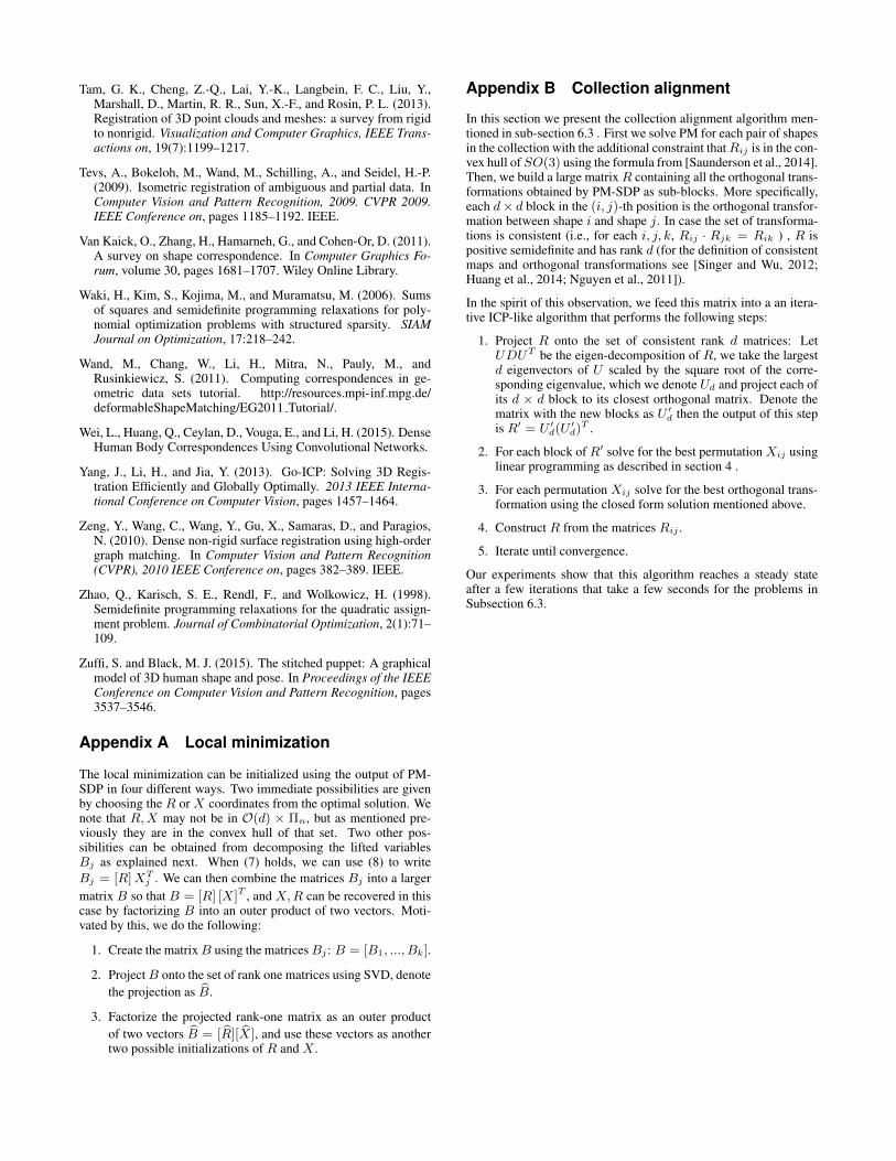
We demonstrate another application of PM-SDP to consistent align-ment of shapes. The task we would like to solve here is the follow-ing: given a set of semantically similar shapes - apply an orthogonaltransformation per shape so that the shapes are aligned. We solvethis problem by using PM-SDP to solve for pairwise orthogonaltransformations and permutations over the entire dataset and thenmodifying the ICP procedure we mentioned in section 4 to projectonto the set of consistent orthogonal transformations; The detailsof the projection procedure and definition of consistency are givenin appendix B. To demonstrate the flexibility of our approach, weuse a variation of the high dimensional embedding used above. Weembedded the shapes into a seven-dimensional space, the first threecoordinates being the euclidian x, y, z coordinates, and the other 4were eigenfunctions of the LB operator (as was done for isomet-ric matching above). Since the Euclidian coordinates should notmix with the eigenfunction coordinates we constrain R to be blockdiagonal.

Intra-subject

Inter-subject

Figure 9: Examples of typical maps obtained with PM-SDP on theFAUST dataset [Bogo et al., 2014]. Top row: intra-subject. Bottomrows: inter-subject. Bottom right: a failure case.

As demonstrated in Figure 13 PM-SDP with d = 7 (secondrow) yielded a better consistent alignment in comparison with themethod for d = 3. The shapes for this experiment are taken fromthree classes of the SHREC07 [Giorgi et al., 2007] dataset. Wemade sure the shapes are arbitrarily rotated, sampled n = k = 20farthest points on each shape and solved for all pairwise matchings;for d = 3 each pair is computed in 2-3 seconds and for d = 7 eachpair takes 15-20 seconds.

Timing. Timing of experiments that appear in the paper have al-ready been stated. Here we provide quantitative timing experi-ments. Figure 14 shows typical run times as a function of dimensionor number of points. The experiments were conducted on randomand noisy synthetic data. In experiment (a) the dimension d variesfrom 3 to 20 and we match k = 50 points to n = 100 points.Experiment (b) compares runtime versus the number of points: ineach experiment we match a k point point cloud to a n = 2k pointpoint cloud (up to k = 50, n = 100) and the dimension is constantd = 10. In both cases, R was constrained to be 5-diagonal and weallowed each point to be matched to 30% of the points in the otherpoint cloud based on prior knowledge (in this case these points wereselected randomly). (c) Shows comparison of the running time ofPM-SDP and the full SDP relaxation discussed in section 3. In thiscase we use d = 10, k = n = 5 . . . 25. Notably, the full relaxationbecomes intractable for more than 17 point, whereas the equivalentPM-SDP formulation solves these problems in just seconds.

Bottom view

Figure 10: Performance on the SCAPE raw scans dataset[Anguelov et al., 2005]. Top left: Cumulative error distribution.Other: Examples of typical maps obtained with PM-SDP . Bottomright: a failure case (forward-backward flip).

Figure 11: Examples of maps obtained with PM-SDP on the non-isometric SHREC07 dataset [Giorgi et al., 2007]. Bottom right: afailure case (incorrect corresponding legs).

7 ConclusionsSummary. We have developed an algorithm that approximatesthe global minimum of the PM problem with a proven exact re-covery property in presence of bilateral symmetries, as well as sev-eral other theoretical properties of the algorithm. We demonstratedstate of the art results for non-rigid isometric and near-isometricshape matching problems solved using our convex relaxation. Wealso showed that PM-SDP is useful for anatomical classification ofshapes and for aligning shape collections.

Limitations. In contrast to previous SDP relaxations of simi-lar problems, we are able to deal with the registration of aroundone hundred points. Nonetheless, in comparison with non-SDPbased approaches, the main limitation of this algorithm remains itstime complexity, which we predict will improve as research on SDPoptimization progresses; another limitation of our shape matchingframework is the fact that spectral embedding is aimed at near-isometric matching, and is not a good model of the problem fornon-isometric shapes.

Future work. One direction we intend to pursue is applying ourtechnique for constructing efficient relaxations for quadratic opti-mization to different problems other than PM. An interesting theo-retical problem which we intend to pursue is proving that PM-SDP(or similar relaxations) give a good approximation of the solution inthe general (noisy, far from exact) case, in contrast with our theoret-ical analysis here which applies only for isometric or near-isometricshapes. Extending to two-way partial matching is also interesting.

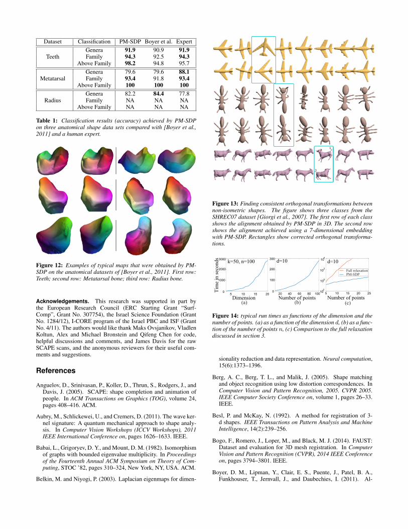
Dataset Classification PM-SDP Boyer et al. ExpertGenera 91.9 90.9 91.9

Teeth Family 94.3 92.5 94.3Above Family 98.2 94.8 95.7

Genera 79.6 79.6 88.1Metatarsal Family 93.4 91.8 93.4

Above Family 100 100 100Genera 82.2 84.4 77.8

Radius Family NA NA NAAbove Family NA NA NA

Table 1: Classification results (accuracy) achieved by PM-SDPon three anatomical shape data sets compared with [Boyer et al.,2011] and a human expert.

Figure 12: Examples of typical maps that were obtained by PM-SDP on the anatomical datasets of [Boyer et al., 2011]. First row:Teeth; second row: Metatarsal bone; third row: Radius bone.

Acknowledgements. This research was supported in part bythe European Research Council (ERC Starting Grant “Surf-Comp”, Grant No. 307754), the Israel Science Foundation (GrantNo. 1284/12), I-CORE program of the Israel PBC and ISF (GrantNo. 4/11). The authors would like thank Maks Ovsjanikov, VladlenKoltun, Alex and Michael Bronstein and Qifeng Chen for code,helpful discussions and comments, and James Davis for the rawSCAPE scans, and the anonymous reviewers for their useful com-ments and suggestions.

References

Anguelov, D., Srinivasan, P., Koller, D., Thrun, S., Rodgers, J., andDavis, J. (2005). SCAPE: shape completion and animation ofpeople. In ACM Transactions on Graphics (TOG), volume 24,pages 408–416. ACM.

Aubry, M., Schlickewei, U., and Cremers, D. (2011). The wave ker-nel signature: A quantum mechanical approach to shape analy-sis. In Computer Vision Workshops (ICCV Workshops), 2011IEEE International Conference on, pages 1626–1633. IEEE.

Babai, L., Grigoryev, D. Y., and Mount, D. M. (1982). Isomorphismof graphs with bounded eigenvalue multiplicity. In Proceedingsof the Fourteenth Annual ACM Symposium on Theory of Com-puting, STOC ’82, pages 310–324, New York, NY, USA. ACM.

Belkin, M. and Niyogi, P. (2003). Laplacian eigenmaps for dimen-

Figure 13: Finding consistent orthogonal transformations betweennon-isometric shapes. The figure shows three classes from theSHREC07 dataset [Giorgi et al., 2007]. The first row of each classshows the alignment obtained by PM-SDP in 3D. The second rowshows the alignment achieved using a 7-dimensional embeddingwith PM-SDP. Rectangles show corrected orthogonal transforma-tions.

5 10 15Dimension

0

1000

2000

3000

Tim

e in

seco

nds k=50, n=100

(a)

20 40 60 80 100Number of points

0

100

200

300 d=10

(b)

5 10 15 20 25Number of points

10-2

100

102

104

Full relaxationPM-SDP

d=10

20

(c)

Figure 14: typical run times as functions of the dimension and thenumber of points. (a) as a function of the dimension d, (b) as a func-tion of the number of points n, (c) Comparison to the full relaxationdiscussed in section 3.

sionality reduction and data representation. Neural computation,15(6):1373–1396.

Berg, A. C., Berg, T. L., and Malik, J. (2005). Shape matchingand object recognition using low distortion correspondences. InComputer Vision and Pattern Recognition, 2005. CVPR 2005.IEEE Computer Society Conference on, volume 1, pages 26–33.IEEE.

Besl, P. and McKay, N. (1992). A method for registration of 3-d shapes. IEEE Transactions on Pattern Analysis and MachineIntelligence, 14(2):239–256.

Bogo, F., Romero, J., Loper, M., and Black, M. J. (2014). FAUST:Dataset and evaluation for 3D mesh registration. In ComputerVision and Pattern Recognition (CVPR), 2014 IEEE Conferenceon, pages 3794–3801. IEEE.

Boyer, D. M., Lipman, Y., Clair, E. S., Puente, J., Patel, B. A.,Funkhouser, T., Jernvall, J., and Daubechies, I. (2011). Al-

gorithms to automatically quantify the geometric similarity ofanatomical surfaces. Proceedings of the National Academy ofSciences, 108(45):18221–18226.

Bronstein, A. M., Bronstein, M. M., and Kimmel, R. (2006). Gen-eralized multidimensional scaling: A framework for isometry-invariant partial surface matching. Proceedings of the Na-tional Academy of Sciences of the United States of America,103(5):1168–1172.

Brown, B. J. and Rusinkiewicz, S. (2007). Global non-rigid align-ment of 3-d scans. ACM Transactions on Graphics (TOG),26(3):21.

Chen, Q. and Koltun, V. (2015). Robust nonrigid registration byconvex optimization. In Proceedings of the IEEE InternationalConference on Computer Vision, pages 2039–2047.

Dym, N. and Lipman, Y. (2016). Exact recovery with symmetriesfor procrustes matching. Technical report.

Eldar, Y., Lindenbaum, M., Porat, M., and Zeevi, Y. Y. (1997). Thefarthest point strategy for progressive image sampling. ImageProcessing, IEEE Transactions on, 6(9):1305–1315.

Fischler, M. A. and Bolles, R. C. (1981). Random sample consen-sus: a paradigm for model fitting with applications to image anal-ysis and automated cartography. Communications of the ACM,24(6):381–395.

Fukuda, M., Kojima, M., Murota, K., and Nakata, K. (2000).Exploiting sparsity in semidefinite programming via matrixcompletion I: General framework. SIAM J. on Optimization,11(3):647–674.

Gelfand, N., Mitra, N. J., Guibas, L. J., and Pottmann, H. (2005).Robust global registration. In Proceedings of the Third Euro-graphics Symposium on Geometry Processing, SGP ’05, Aire-la-Ville, Switzerland, Switzerland. Eurographics Association.

Giorgi, D., Biasotti, S., and Paraboschi, L. (2007). Shape retrievalcontest 2007: Watertight models track. SHREC competition, 8.

Gower, J. C. and Dijksterhuis, G. B. (2004). Procrustes problems,volume 3. Oxford University Press Oxford.

Grone, R., Johnson, C. R., Sa, E. M., and Wolkowicz, H. (1984).Positive definite completions of partial Hermitian matrices. Lin-ear algebra and its applications, 58:109–124.

Huang, Q., Wang, F., and Guibas, L. (2014). Functional map net-works for analyzing and exploring large shape collections. ACMTrans. Graph., 33(4):36:1–36:11.

Jain, V., Zhang, H., and Van Kaick, O. (2007). Non-Rigid SpectralCorrespondence of Triangle Meshes. International Journal ofShape Modeling, 13:101–124.

Kendall, D. G. (1984). Shape manifolds, Procrustean metrics, andcomplex projective spaces. Bulletin of the London MathematicalSociety, 16(2):81–121.

Kezurer, I., Kovalsky, S. Z., Basri, R., and Lipman, Y. (2015). Tightrelaxation of quadratic matching. Computer Graphics Forum,34(5):115–128.

Kim, V. G., Lipman, Y., and Funkhouser, T. (2011). Blended intrin-sic maps. ACM Transactions on Graphics, 30(4):1.

Leordeanu, M. and Hebert, M. (2005). A spectral technique for cor-respondence problems using pairwise constraints. In ComputerVision, 2005. ICCV 2005. Tenth IEEE International Conferenceon, volume 2, pages 1482–1489. IEEE.

Li, H., Sumner, R. W., and Pauly, M. (2008). Global correspon-dence optimization for non-rigid registration of depth scans. InComputer Graphics Forum, volume 27, pages 1421–1430. WileyOnline Library.

Lipman, Y. and Funkhouser, T. (2009). Mobius voting for surfacecorrespondence. In ACM Transactions on Graphics (TOG), vol-ume 28, page 72. ACM.

Luo, Z.-Q., Ma, W.-k., So, A. M.-C., Ye, Y., and Zhang, S. (2010).Semidefinite relaxation of quadratic optimization problems. Sig-nal Processing Magazine, IEEE, 27(3):20–34.

Memoli, F. and Sapiro, G. (2004). Comparing point clouds. InProceedings of the 2004 Eurographics/ACM SIGGRAPH Sym-posium on Geometry Processing, SGP ’04, pages 32–40, NewYork, NY, USA. ACM.

Mitteroecker, P. and Gunz, P. (2009). Advances in geometric mor-phometrics. Evolutionary Biology, 36(2):235–247.

MOSEK (2015). The MOSEK optimization toolbox for MATLABmanual. Version 7.1 (Revision 49).

Nguyen, A., Ben-Chen, M., Welnicka, K., Ye, Y., and Guibas, L.(2011). An optimization approach to improving collections ofshape maps. Computer Graphics Forum, 30(5):1481–1491.

Ovsjanikov, M., Ben-Chen, M., Solomon, J., Butscher, A., andGuibas, L. (2012). Functional maps: a flexible representation ofmaps between shapes. ACM Transactions on Graphics (TOG),31(4):30.

Ovsjanikov, M., Merigot, Q., Memoli, F., and Guibas, L. (2010).One point isometric matching with the heat kernel. In ComputerGraphics Forum, volume 29, pages 1555–1564. Wiley OnlineLibrary.

Ovsjanikov, M., Sun, J., and Guibas, L. (2008). Global intrinsicsymmetries of shapes. In Computer Graphics Forum, volume 27,pages 1341–1348. Wiley Online Library.

Pinkall, U. and Polthier, K. (1993). Computing discrete mini-mal surfaces and their conjugates. Experimental mathematics,2(1):15–36.

Pokrass, J., Bronstein, A. M., Bronstein, M. M., Sprechmann, P.,and Sapiro, G. (2013). Sparse modeling of intrinsic correspon-dences. Computer Graphics Forum, 32(2 PART4):459–468.

Poljak, S., Rendl, F., and Wolkowicz, H. (1995). A recipe forsemidefinite relaxation for (0, 1)-quadratic programming. Jour-nal of Global Optimization, 7(1):51–73.

Rusinkiewicz, S. and Levoy, M. (2001). Efficient variants of theICP algorithm. Proceedings Third International Conference on3-D Digital Imaging and Modeling, pages 145–152.

Rustamov, R. M. (2007). Laplace-Beltrami eigenfunctions for de-formation invariant shape representation. In Proceedings of theFifth Eurographics Symposium on Geometry Processing, SGP’07, pages 225–233, Aire-la-Ville, Switzerland, Switzerland. Eu-rographics Association.

Saunderson, J., Parrilo, P. A., and Willsky, A. S. (2014). Semidef-inite descriptions of the convex hull of rotation matrices. arXivpreprint arXiv:1403.4914.

Singer, A. and Wu, H.-T. (2012). Vector diffusion maps and theconnection laplacian. Communications on Pure and AppliedMathematics, 65(8):1067–1144.

Tam, G. K., Cheng, Z.-Q., Lai, Y.-K., Langbein, F. C., Liu, Y.,Marshall, D., Martin, R. R., Sun, X.-F., and Rosin, P. L. (2013).Registration of 3D point clouds and meshes: a survey from rigidto nonrigid. Visualization and Computer Graphics, IEEE Trans-actions on, 19(7):1199–1217.

Tevs, A., Bokeloh, M., Wand, M., Schilling, A., and Seidel, H.-P.(2009). Isometric registration of ambiguous and partial data. InComputer Vision and Pattern Recognition, 2009. CVPR 2009.IEEE Conference on, pages 1185–1192. IEEE.

Van Kaick, O., Zhang, H., Hamarneh, G., and Cohen-Or, D. (2011).A survey on shape correspondence. In Computer Graphics Fo-rum, volume 30, pages 1681–1707. Wiley Online Library.

Waki, H., Kim, S., Kojima, M., and Muramatsu, M. (2006). Sumsof squares and semidefinite programming relaxations for poly-nomial optimization problems with structured sparsity. SIAMJournal on Optimization, 17:218–242.

Wand, M., Chang, W., Li, H., Mitra, N., Pauly, M., andRusinkiewicz, S. (2011). Computing correspondences in ge-ometric data sets tutorial. http://resources.mpi-inf.mpg.de/deformableShapeMatching/EG2011 Tutorial/.

Wei, L., Huang, Q., Ceylan, D., Vouga, E., and Li, H. (2015). DenseHuman Body Correspondences Using Convolutional Networks.

Yang, J., Li, H., and Jia, Y. (2013). Go-ICP: Solving 3D Regis-tration Efficiently and Globally Optimally. 2013 IEEE Interna-tional Conference on Computer Vision, pages 1457–1464.

Zeng, Y., Wang, C., Wang, Y., Gu, X., Samaras, D., and Paragios,N. (2010). Dense non-rigid surface registration using high-ordergraph matching. In Computer Vision and Pattern Recognition(CVPR), 2010 IEEE Conference on, pages 382–389. IEEE.

Zhao, Q., Karisch, S. E., Rendl, F., and Wolkowicz, H. (1998).Semidefinite programming relaxations for the quadratic assign-ment problem. Journal of Combinatorial Optimization, 2(1):71–109.

Zuffi, S. and Black, M. J. (2015). The stitched puppet: A graphicalmodel of 3D human shape and pose. In Proceedings of the IEEEConference on Computer Vision and Pattern Recognition, pages3537–3546.

Appendix A Local minimization

The local minimization can be initialized using the output of PM-SDP in four different ways. Two immediate possibilities are givenby choosing the R or X coordinates from the optimal solution. Wenote that R,X may not be in O(d) × Πn, but as mentioned pre-viously they are in the convex hull of that set. Two other pos-sibilities can be obtained from decomposing the lifted variablesBj as explained next. When (7) holds, we can use (8) to writeBj = [R]XT

j . We can then combine the matrices Bj into a largermatrix B so that B = [R] [X]T , and X,R can be recovered in thiscase by factorizing B into an outer product of two vectors. Moti-vated by this, we do the following:

1. Create the matrixB using the matricesBj : B = [B1, ..., Bk].

2. ProjectB onto the set of rank one matrices using SVD, denotethe projection as B.

3. Factorize the projected rank-one matrix as an outer productof two vectors B = [R][X], and use these vectors as anothertwo possible initializations of R and X .

Appendix B Collection alignment

In this section we present the collection alignment algorithm men-tioned in sub-section 6.3 . First we solve PM for each pair of shapesin the collection with the additional constraint thatRij is in the con-vex hull of SO(3) using the formula from [Saunderson et al., 2014].Then, we build a large matrixR containing all the orthogonal trans-formations obtained by PM-SDP as sub-blocks. More specifically,each d× d block in the (i, j)-th position is the orthogonal transfor-mation between shape i and shape j. In case the set of transforma-tions is consistent (i.e., for each i, j, k, Rij · Rjk = Rik ) , R ispositive semidefinite and has rank d (for the definition of consistentmaps and orthogonal transformations see [Singer and Wu, 2012;Huang et al., 2014; Nguyen et al., 2011]).

In the spirit of this observation, we feed this matrix into a an itera-tive ICP-like algorithm that performs the following steps:

1. Project R onto the set of consistent rank d matrices: LetUDUT be the eigen-decomposition of R, we take the largestd eigenvectors of U scaled by the square root of the corre-sponding eigenvalue, which we denote Ud and project each ofits d × d block to its closest orthogonal matrix. Denote thematrix with the new blocks as U ′d then the output of this stepis R′ = U ′d(U

′d)T .

2. For each block of R′ solve for the best permutation Xij usinglinear programming as described in section 4 .

3. For each permutation Xij solve for the best orthogonal trans-formation using the closed form solution mentioned above.

4. Construct R from the matrices Rij .

5. Iterate until convergence.

Our experiments show that this algorithm reaches a steady stateafter a few iterations that take a few seconds for the problems inSubsection 6.3.