Journal of Algebra 331 (2011) 304–310

Contents lists available at ScienceDirect

Journal of Algebra

www.elsevier.com/locate/jalgebra

Point-line collinearity graphs of two sporadic minimalparabolic geometries

Peter Rowley, Paul Taylor ∗

School of Mathematics, University of Manchester, Oxford Road, Manchester M13 6PL, UK

a r t i c l e i n f o a b s t r a c t

Article history:Received 16 June 2010Available online 12 January 2011Communicated by Derek Holt

MSC:20D08

Keywords:Minimal parabolic geometryPoint-line collinearity graphSporadic simple groups

The disc structure of the point-line collinearity graph for the ranktwo minimal parabolic geometries of the Thompson and Harada–Norton simple groups are investigated. Additionally details of thesub-orbits of these two groups in their conjugation action upon aninvolution conjugacy class is given. In particular, we give a list ofrepresentatives for each of these sub-orbits.

© 2011 Elsevier Inc. All rights reserved.

1. Introduction

This paper reports the outcome of calculations carried out on the point-line collinearity graphs fortwo sporadic minimal parabolic geometries. Both of these geometries have rank two and are of char-acteristic two. One of these geometries is associated with Th, Thompson’s simple group and the otherwith HN, the Harada–Norton simple group. Apart from their intrinsic interest, the principal motivationfor these investigations is that each of these graphs occur as full subgraphs of the Monster graph –see [6–8]. As a consequence the data assembled here will prove extremely valuable in unpicking someof the intricacies of the Monster graph, a graph associated with the Monster simple group which hasapproximately 5 × 1027 vertices.

The geometries Γ we study here were first described in [5] in terms of the coset geometry ofcertain 2-minimal subgroups. So Γ = Γ0 ∪ Γ1 where Γ0 is the set of points of Γ and Γ1 is the setof lines, with an incidence relation ∗. The point-line collinearity graph, G , of Γ has V (G) = Γ0 as its

* Corresponding author.E-mail addresses: peter.j.rowley@manchester.ac.uk (P. Rowley), p.taylor@maths.manchester.ac.uk (P. Taylor).

0021-8693/$ – see front matter © 2011 Elsevier Inc. All rights reserved.doi:10.1016/j.jalgebra.2010.11.022

P. Rowley, P. Taylor / Journal of Algebra 331 (2011) 304–310 305

vertex set with x, y ∈ Γ0 adjacent provided x �= y and for some � ∈ Γ1, x ∗ � and y ∗ �. The usual graphtheoretic distance on G will be denoted by d( , ), and for i ∈ N ∪ {0} and x ∈ Γ0 define

�i(x) = {y ∈ Γ0

∣∣ d(x, y) = i}.

We refer to �i(x) as the ith disc of x. Clearly �i(x) is a union of certain Gx-orbits of Γ0. It is thesediscs we examine here. For more background details on these geometries and any unexplained termi-nology, consult [5]. And for related geometries, see [2]

Our first result concerns the point-line collinearity graph associated with Th – this graph has976,841,775 vertices, which may be identified with a certain conjugacy class of Th.

Theorem 1. Suppose that G ∼= Th and G is the point-line collinearity graph of the characteristic 2 minimalparabolic geometry for G. Then G has permutation rank 38 on V (G), G has diameter 5 and for t ∈ V (G) wehave

(i) |�1(t)| = 270 with �1(t) a Gt -orbit;(ii) |�2(t)| = 64800, �2(t) consisting of two Gt -orbits;

(iii) |�3(t)| = 15060480, �3(t) consisting of six Gt -orbits;(iv) |�4(t)| = 858497006, �4(t) consisting of twenty six Gt -orbits; and(v) |�5(t)| = 103219200, �5(t) consisting of two Gt -orbits.

The second graph we look at has fewer vertices, namely 74,064,375, and again the vertices maybe identified with a conjugacy class of HN.

Theorem 2. Suppose that G ∼= HN and G is the point-line collinearity graph of the characteristic 2 minimalparabolic geometry for G. Then G has permutation rank 71 on V (G), G has diameter 5 and for t ∈ V (G) wehave

(i) |�1(t)| = 150 with �1(t) a Gt -orbit;(ii) |�2(t)| = 17760, �2(t) consisting of three Gt -orbits;

(iii) |�3(t)| = 1638400, �3(t) consisting of eight Gt -orbits;(iv) |�4(t)| = 68721664, �4(t) consisting of fifty five Gt -orbits; and(v) |�5(t)| = 3686400, �5(t) consisting of three Gt -orbits.

The information summarized in Theorems 1 and 2 was obtained with the assistance of Magma [3]using matrix representatives for Th and HN supplied by [10]. For the description of groups and thenames of conjugacy classes we follow the Atlas [4]. If x is a point in either of these two geometries,then it is the case that Gx = CG(ix) where ix is an involution of G and Z(Gx) = 〈ix〉. Thus we mayidentify Γ0 with X = iG

x . For G ∼= Th, X is the conjugacy class 2A, while for G ∼= HN it is the conjugacyclass 2B . So for the former group Gx = CG(ix) ∼ 21+8+ A9 and for the latter Gx = CG(ix) ∼ 21+8+ ×(A5 × A5).2. Under this translation, for points x, y ∈ Γ0 and ix, i y the corresponding involutions, x andy are adjacent in G if and only if i y ∈ O 2(CG(ix)). Thus �1(x) becomes (X ∩ O 2(CG(ix))) \ {ix}. It isin this arena that we uncover the structure of the discs of the point-line collinearity graph. The sub-orbits of G in its conjugation action on X form an important part of our investigation and involvesanalyzing the sets XC defined by

XC = {x ∈ X | tx ∈ C},for C a conjugacy class of G and t a fixed element of X . Clearly each non-empty set XC is a unionof certain CG(t)-orbits. The sizes of these sets for each C can easily be determined from the complexcharacter table of G . In Section 2 further details are given as to how our calculations were per-formed. Section 3 defines collapsed adjacency matrices. The collapsed adjacency matrices for thesetwo collinearity graphs, from which Theorems 1 and 2 readily follow, are available as supplementary

306 P. Rowley, P. Taylor / Journal of Algebra 331 (2011) 304–310

material to this paper. Finally, in Section 4, suborbit representatives are listed for the action of Thand HN on the vertices of these two graphs. A computer file containing these representatives may beobtained from the first named author on request.

2. Determining the CG (t)-orbits

2.1. G ∼= Th

Much of the methodology for obtaining orbit representatives in this case follows the work donein [9].

We employ the 248-dimensional GF(2)-representation of Th provided in [10]. Let a,b be the stan-dard generators for G given there, where a is in class 2A, b is in class 3A and ab has order 19. Weset t = a, and take X to be the conjugacy class 2A. Then generators for the maximal subgroup CG(t),of shape 21+8+ .A9, can be obtained from the straight line program available in [10].

We set Q = O 2(CG(t)). So Q ∼= 21+8+ � CG(t). Generators for Q can easily be obtained by tak-ing random elements of CG(t) until we find elements having order 36 and taking their 9th powers,enough of which along with t will generate Q .

Direct computation in CG(t) is precluded by its size and the large degree of the representation.However, since Q is small and a normal subgroup, we may construct explicitly the conjugation actionof CG(t) on Q , giving us (after relabelling the elements of Q as {1,. . . ,512}) a homomorphism ϕ :CG (t) → M � Sym(512) with M ∼= CG(t)/〈t〉. With this set up in place, we describe how we go aboutfinding representatives for the CG(t)-orbits of X .

From information gleaned from the character table, we know that X consists of thirty-eight CG(t)-orbits across 29 non-empty sets XC of known size. So we know that at least twenty of the non-empty sets XC each consist of a single CG(t)-orbit, and at most nine sets XC split into two or moreCG (t)-orbits. Our strategy is to take a random conjugate x of t , determine the class of z = tx andso which XC contains the orbit, and where possible the size of CCG (t)(x). This then yields the sizeof the orbit and eventually helps in finding representatives for all thirty-eight CG(t)-orbits. The classof z is generally immediately apparent from its order and the dimension of its fixed space on the248-dimensional GF(2)-module V , so we focus on the second task: determining the size of CCG (t)(x).

Since CCG (t)(x) � CG(z), if we can compute CG (z) and if it is sufficiently small, we can then findCCG (t)(x) directly in this group. In particular, where z is in classes 18B,19A,20A,21A,27A,28A,36A,we find CG(z) = 〈z〉 and so this is easily done. When z is in a class of order 3 we can computeCG (z) using [1] (and when z has order 3n for some n > 1 we can compute its centralizer insideCG (zn) which we find by the same method). Finally, when z is in class C = 13A, we observe thatCG (z) has order 39, so CCG (t)(x) must have order 1 or 3 (since 13 does not divide |CG(t)|). But |XC | =30965760 = |CG(t)|/3, and this forces |CCG (t)(x)| to have size 3, so we know X13A is a single CG(t)-orbit.

Now suppose C is a class of elements of even order 2m. Here we have the advantage that zm isan involution commuting with t and x, as t inverts z, so zm ∈ CCG (t)(x) = CCG (t)(z) � CCG (t)(zm). Recallthat we have CG(t)/〈t〉 ∼= M � Sym(512) corresponding to the conjugation action of CG (t) on Q . Nowwe have ϕ : CG(t) → M explicitly, so we can calculate CM(ϕ(zm)), take its inverse image, and if itis sufficiently small, calculate CCG (t)(x) in this. Further, since Q is small, we can compute C Q (x) �

CCG (t)(x). Since the points of M correspond to the elements of Q , we can form Sx , the stabilizer inM of the subset of {1, . . . ,512} corresponding to C Q (x). Then CCG (t)(x) must lie in its inverse image.In all cases where z has even order, we find that Sx ∩ CM(φ(zm)) is sufficiently small to be able tocompute CCG (t)(x) in its inverse image.

These calculations are sufficient to uncover nine sets XC that each split into two CG(t)-orbits. Sowe conclude that the remaining unanalysed XC (namely X5A, X7A ) are single orbits.

2.2. G ∼= HN

Finding representatives for the CG(t)-orbits when G ∼= HN, t ∈ X where X is the 2B conjugacyclass of HN poses a different set of problems to those encountered in the Thompson group. In par-

P. Rowley, P. Taylor / Journal of Algebra 331 (2011) 304–310 307

ticular, here we have that CG(t) is relatively small, containing just 3,686,400 elements (recall thatCG(t) ∼ 21+8+ (A5 × A5).2). This means computation inside CG(t) can be carried out directly in the ma-trix group, as can CG(t)-conjugacy testing, making the discovery of new orbits and their sizes mucheasier. (We use the representation of G as 132 × 132 matrices over GF(4) from [10].) On the otherhand, there are more CG(t)-orbits to find: 70 orbits across 47 non-empty XC , and many classes of Gcannot be identified so easily by the dimensions of their fixed spaces on the 132-dimensional moduleV . Therefore our strategy is as follows.

We take a random conjugate x of t , and compute four easily-determined orbit invariants: theorder of z = tx, the dimension of the fixed space of z, the value dx = dim(CV (t) ∩ CV (x)) and theorder of CCG (t)(x) (and hence the size of the orbit). From the sets XC we know if we have found allthe orbits for a particular order of z and if this is the case the representative is discarded. Otherwise,we test whether the representative is CG(t)-conjugate to any representative sharing its invariants thatwe have already found and if not add it to our list. (This conjugacy testing is initially carried outusing Magma’s IsConjugate command, but as this has been found to be fallible in this situationthe results are confirmed by other methods.) We leave determining the exact class in which z liesuntil after all the representatives have been found.

When a representative x for a new orbit is found we also form its ‘powers’ tzn for all valuesof n dividing the order of z = tx, and check these as well. Suppose we have an element x ∈ XC forsome class C of G . Further suppose that for z ∈ C , (zn)G = D (C ‘powers down’ to D). Then we havex′ = tzn = xtx . . . tx ∈ X . Clearly tx′ ∈ D and so x′ ∈ XD . Further, all elements from a particular CG(t)-orbit in XC power down in this fashion to the same orbit in XD . Since the smaller CG (t)-orbits tendto lie in XC for classes C having elements of small orders, this powering down strategy can prove veryhelpful in unearthing these elusive orbits. We note that forming an x′ in this manner also furnishesus with a conjugating element h such that th = x′ in terms of t and the element g conjugating tto x, reducing the number and length of words needed to obtain representatives for every orbit.We observe that we can define representatives for all seventy CG(t)-orbits using only 34 words (seeSection 4.2).

3. Collapsed adjacency matrices

Once we have a list of representatives and conjugating elements for the CG(t)-orbits, we determinethe collapsed adjacency matrix for the point-line collinearity graphs. Recall that each disc of the graphis a union of Gt -orbits (which we view as CG(t)-orbits on X ). The collapsed adjacency matrix has onesuch orbit associated with each row and with each column. Then the (i, j)th entry of the matrix givesthe number of edges going from a particular arbitrary point in the associated orbit Oi to any point inthe associated orbit O j .

Our first task in constructing this matrix is to create an explicit listing of the elements of �1(t) =X ∩ O 2(CG(t)). This is easily done in both cases. (Note that for G ∼= T h, the group O 2(CG(t)) is justthe group Q described in Section 2.1.) Then for each CG(t)-orbit representative x and conjugatingelement g (so t g = x, see Section 4), we compute �1(x) = �1(t)g . We determine in which orbit eachelement of �1(x) lies, and so build a ‘neighbourhood profile’ for every orbit. From this data it issimple to locate which disc a given orbit is in, and to create the collapsed adjacency matrix.

Orbits in the matrix are ordered first in terms of increasing distance from t and then in terms ofincreasing size. See the supplementary material for these matrices.

4. Sub-orbit representatives

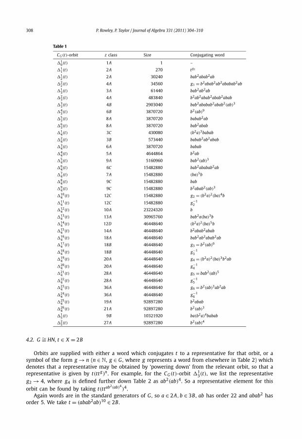
4.1. G ∼= Th, t ∈ X = 2A

Let a,b be the standard generators of G , so that a ∈ 2A, b ∈ 3A and ab ∈ 19A. We set t = a.For each CG(t)-orbit of X , we give the class of z = tx for an element x in that orbit, and a word in

a and b conjugating t to a representative element for that orbit. Some words refer to an element gi

which will be defined elsewhere in Table 1.

308 P. Rowley, P. Taylor / Journal of Algebra 331 (2011) 304–310

Table 1

CG (t)-orbit z class Size Conjugating word

�10(t) 1A 1 –

�11(t) 2A 270 t g1

�12(t) 2A 30240 bab2abab2ab

�22(t) 4A 34560 g1 = b2abab2ab2ababab2ab

�13(t) 3A 61440 bab2ab2ab

�23(t) 4A 483840 b2ab2abab2abab2abab

�33(t) 4B 2903040 bab2ababab2abab2(ab)3

�43(t) 6B 3870720 b2(ab)9

�53(t) 8A 3870720 babab2ab

�63(t) 8A 3870720 bab2abab

�14(t) 3C 430080 (b2a)3babab

�24(t) 3B 573440 babab2ab2abab

�34(t) 6A 3870720 babab

�44(t) 5A 4644864 b2ab

�54(t) 9A 5160960 bab2(ab)3

�64(t) 6C 15482880 bab2ababab2ab

�74(t) 7A 15482880 (ba)5b

�84(t) 9C 15482880 bab

�94(t) 9C 15482880 b2abab2(ab)3

�104 (t) 12C 15482880 g2 = (b2a)2(ba)4b

�114 (t) 12C 15482880 g−1

2

�124 (t) 10A 23224320 b

�134 (t) 13A 30965760 bab2a(ba)3b

�144 (t) 12D 46448640 (b2a)2(ba)5b

�154 (t) 14A 46448640 b2abab2abab

�164 (t) 18A 46448640 bab2ab2abab2ab

�174 (t) 18B 46448640 g3 = b2(ab)6

�184 (t) 18B 46448640 g−1

3

�194 (t) 20A 46448640 g4 = (b2a)2(ba)3b2ab

�204 (t) 20A 46448640 g−1

4

�214 (t) 28A 46448640 g5 = bab2(ab)5

�224 (t) 28A 46448640 g−1

5

�234 (t) 36A 46448640 g6 = b2(ab)3ab2ab

�244 (t) 36A 46448640 g−1

6

�254 (t) 19A 92897280 b2abab

�264 (t) 21A 92897280 b2(ab)3

�15(t) 9B 10321920 ba(b2a)4babab

�25(t) 27A 92897280 b2(ab)4

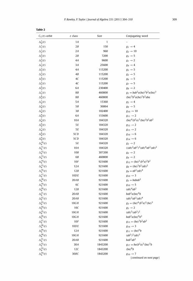
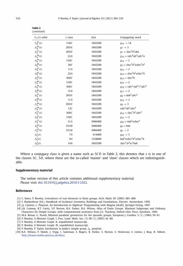
4.2. G ∼= HN, t ∈ X = 2B

Orbits are supplied with either a word which conjugates t to a representative for that orbit, or asymbol of the form g → n (n ∈ N, g ∈ G , where g represents a word from elsewhere in Table 2) whichdenotes that a representative may be obtained by ‘powering down’ from the relevant orbit, so that arepresentative is given by t(tt g)n . For example, for the CG (t)-orbit �1

3(t), we list the representativeg2 → 4, where g4 is defined further down Table 2 as ab2(ab)4. So a representative element for thisorbit can be found by taking t(ttab2(ab)4

)4.Again words are in the standard generators of G , so a ∈ 2A,b ∈ 3B , ab has order 22 and abab2 has

order 5. We take t = (abab2ab)10 ∈ 2B .

P. Rowley, P. Taylor / Journal of Algebra 331 (2011) 304–310 309

Table 2

CG (t)-orbit z class Size Conjugating word

�10(t) 1A 1 –

�11(t) 2B 150 g1 → 4

�12(t) 2A 960 g2 → 10

�22(t) 2B 7200 g3 → 5

�32(t) 4A 9600 g1 → 2

�13(t) 3A 25600 g4 → 4

�23(t) 4A 115200 g5 → 5

�33(t) 4B 115200 g2 → 5

�43(t) 4C 115200 g6 → 5

�53(t) 4C 115200 g7 → 5

�63(t) 6A 230400 g8 → 2

�73(t) 8B 460800 g1 = bab2a(ba)2b2a(ba)3

�83(t) 8B 460800 (ba)3b2a(ba)2b2aba

�14(t) 5A 15360 g2 → 4

�24(t) 5B 36864 g9 → 5

�34(t) 3B 102400 g10 → 10

�44(t) 6A 153600 g11 → 2

�54(t) 10A 184320 (ba)4(b2a)3(ba)2b2ab2

�64(t) 5E 184320 g12 → 2

�74(t) 5E 184320 g13 → 2

�84(t) 5C D 184320 g10 → 6

�94(t) 5C D 184320 g14 → 6

�104 (t) 5E 184320 g3 → 2

�114 (t) 10A 184320 ((ab)2ab2)2(ab)4ab2(ab)2

�124 (t) 10B 307200 g2 → 2

�134 (t) 6B 460800 g4 → 2

�144 (t) 10F 921600 g12 = (ba)2(b2a)2b2

�154 (t) 12A 921600 g8 = (ba)3b2(ab)2

�164 (t) 12B 921600 g4 = ab2(ab)4

�174 (t) 10D E 921600 g10 → 3

�184 (t) 20AB 921600 g5 = babab2

�194 (t) 6C 921600 g10 → 5

�204 (t) 12B 921600 (ab)4ab2

�214 (t) 20AB 921600 bab2a(ba)4b

�224 (t) 20AB 921600 (ab)2ab2(ab)4

�234 (t) 10G H 921600 g3 = (ba)4(b2a)2(ba)3

�244 (t) 10C 921600 g5 → 2

�254 (t) 10G H 921600 (ab)5(ab2)2

�264 (t) 10G H 921600 bab2a(ba)6b2

�274 (t) 10F 921600 g13 = (ba)3b2ab2

�284 (t) 10D E 921600 g14 → 3

�294 (t) 12A 921600 g11 = (ba)6b

�304 (t) 10G H 921600 (ab2)2(ab)5

�314 (t) 20AB 921600 bab2ab2

�324 (t) 30A 1843200 g17 = ba(b2a)3(ba)3b

�334 (t) 12C 1843200 (ba)8b

�344 (t) 30BC 1843200 g10 → 7

(continued on next page)

310 P. Rowley, P. Taylor / Journal of Algebra 331 (2011) 304–310

Table 2(continued)

CG (t)-orbit z class Size Conjugating word

�354 (t) 15BC 1843200 g10 → 14

�364 (t) 20D E 1843200 g7 → 3

�374 (t) 20D E 1843200 g7 = (ba)2b2aba

�384 (t) 22A 1843200 g16 = (ab)4ab2(ab)2a

�394 (t) 15BC 1843200 g14 → 2

�404 (t) 20C 1843200 g2 = (ba)3b2a(ba)5b2

�414 (t) 11A 1843200 g16 → 2

�424 (t) 22A 1843200 g18 = (ba)2b2a(ba)3b

�434 (t) 30BC 1843200 g14 = (ba)4b

�444 (t) 15BC 1843200 g10 → 2

�454 (t) 30BC 1843200 g10 = (ab)2(ab2)2(ab)5

�464 (t) 15A 1843200 g17 → 2

�474 (t) 20D E 1843200 g6 = bab2(ab)2

�484 (t) 11A 1843200 g18 → 2

�494 (t) 20D E 1843200 g6 → 3

�504 (t) 12C 1843200 (ab)2ab2(ab)5

�514 (t) 30BC 1843200 g19 = (ba)7b2(ab)2

�524 (t) 15BC 1843200 g19 → 2

�534 (t) 21A 3686400 g20 = bab2a(ba)4

�544 (t) 25AB 3686400 g9 = bab

�554 (t) 25AB 3686400 g9 → 2

�15(t) 7A 614400 g20 → 3

�25(t) 9A 1228800 bab2a(ba)2b2a(ba)4b

�35(t) 14A 1843200 (ba)2(b2a)2bab

Where a conjugacy class is given a name such as 5C D in Table 2, this denotes that z is in one ofthe classes 5C , 5D , where these are the so-called ‘master’ and ‘slave’ classes which are indistinguish-able.

Supplementary material

The online version of this article contains additional supplementary material.Please visit doi:10.1016/j.jalgebra.2010.11.022.

References

[1] C. Bates, P. Rowley, Centralizers of real elements in finite groups, Arch. Math. 85 (2005) 485–489.[2] F. Buekenhout (Ed.), Handbook of Incidence Geometry, Buildings and Foundations, Elsevier, Amsterdam, 1995.[3] J.J. Cannon, C. Playoust, An Introduction to Algebraic Programming with Magma [draft], Springer-Verlag, 1997.[4] J.H. Conway, R.T. Curtis, S.P. Norton, R.A. Parker, R.A. Wilson, Atlas of Finite Groups. Maximal Subgroups and Ordinary

Characters for Simple Groups, with computational assistance from J.G. Thackray, Oxford Univ. Press, Eynsham, 1985.[5] M.A. Ronan, G. Stroth, Minimal parabolic geometries for the sporadic groups, European J. Combin. 5 (1) (1984) 59–91.[6] P. Rowley, A Monster Graph. I, Proc. Lond. Math. Soc. (3) 90 (1) (2005) 42–60.[7] P. Rowley, A Monster Graph. II, unpublished manuscript.[8] P. Rowley, A Monster Graph. III, unpublished manuscript.[9] P. Rowley, P. Taylor, Involutions in Janko’s simple group J4, preprint.

[10] R.A. Wilson, P. Walsh, J. Tripp, I. Suleiman, S. Rogers, R. Parker, S. Norton, S. Nickerson, S. Linton, J. Bray, R. Abbott,http://brauer.maths.qmul.ac.uk/Atlas/.