Poaching Workers in a Supply Chain: Enemy from Within? · Electronic copy available at : http ://ssrn.com /abstract = 2560084 Poaching Workers in a Supply Chain: Enemy from Within?

Electronic copy available at: http://ssrn.com/abstract=2560084

Poaching Workers in a Supply Chain: Enemy fromWithin?

Evan Barlow, Gad Allon, Achal BassambooKellogg School of Management, Northwestern University, Evanston, Illinois 60208

[email protected], [email protected], [email protected]

Poaching is the prevalent practice of recruiting workers who are already employed elsewhere. Economy-wide,

it represents the primary mode by which workers flow directly from one firm to another. In this paper, we

examine the interaction between the flow of goods and the flow of workers (via poaching) between firms

linked in a supply chain. We find that the direction of worker poaching between supply chain partners can

run counter to classical labor economics results. Specifically, in a supply chain, the less productive firm may

offer its workers higher wages and poach workers from the more productive firm. We also find that worker

flows accomplished via poaching impact supply chain management. First, we find that the identity of supply

chain bottleneck may depend on whether poaching is available as a means to accomplish worker flows. Next,

we find that the benefits of worker flows between supply chain partners in some cases outweigh the costs

incurred, so no-poaching agreements would be worse for some supply chains. This net benefit of poaching

between members of a supply chain is robust to the presence of outside labor market competitors as long

as the competitors do not have high productivity. Thus, poaching workers from supply chain partners can

often increase the benefit of operating in manufacturing hubs for all supply chain members.

Key words : worker poaching, passive recruiting, supply chain, capacity management, staffing

1. Introduction

To escape the costs of finding, recruiting, hiring, and training workers, firms often resort

to poaching workers. Worker poaching is the practice of actively recruiting workers who

are already employed elsewhere. Examples of poaching are prevalent in many industries,

including tech, consulting, insurance, finance, law, services, manufacturing, and customer

support. In fact, Fallick and Fleischman (2001) found that in the late 1990’s, poaching

accounted for about 80% of all job-to-job transitions. Only one-fifth of all survey respon-

dents who switched jobs were even searching for a new job. More recently, Jones, et al.

(2011) surveyed managers at firms that received stimulus funds through the American

Recovery and Reinvestment Act, a legislation designed in part to combat the escalating

unemployment crisis during the Great Recession. The authors found that more stimulus

funds had actually been spent poaching workers instead of hiring and training the unem-

ployed.

1

Electronic copy available at: http://ssrn.com/abstract=2560084

Barlow, Allon, and Bassamboo: Poaching Workers in a Supply Chain2

The practice of poaching is becoming even easier as social and professional networks and

job search websites develop innovative recruiting solutions. LinkedIn, GlassDoor, Career-

Builder, and Monster all offer services aimed at finding the best candidates to fulfill a

firm’s needs. They can even provide insight into which workers are most likely to accept

an offer and the salary range that would be required to entice workers to leave their cur-

rent employer. Some even offer a platform to communicate with prospects confidentially.

With these novel approaches to recruiting, poaching is likely to become even more widely

practiced.

With the prevalence of poaching, it is to be expected among competitors or peers.

However, it is also quite prevalent among partners of the same value chain, or supply

chain. While poaching from a partner could be perceived as damaging to the business

relationship, the economic impact of such a practice is an open question.

We argue in this paper that poaching between members of a supply chain has the

potential to actually improve supply chain performance and benefit both suppliers and cus-

tomers. A simple example of potential benefits of poaching between supply chain partners

comes from the shale oil and gas industry, which has become a key supplier for the energy,

chemicals, and plastics industries. Shale oil and gas exploration, drilling, and extraction are

very labor intense; and the young industry has expanded rapidly, forcing firms to employ

very aggressive recruiting strategies. As evidence, the median starting salary of recent grad-

uates from the South Dakota School of Mines and Technology is higher than that of recent

graduates from Stanford, Harvard, or any other Ivy League school (PayScale Inc. 2014). To

satisfy their skilled labor requirements, shale extraction firms resort to poaching machin-

ists, mechanics, and those with experience in handling chemicals and operating industrial

equipment from their customers in plastics and chemicals (Olson et al. 2013). The majority

of the workers currently employed in shale oil and gas came from other industries, and

many of them were poached. This new industry that has acquired so many workers via

poaching is having a large economic impact: BCG estimates that the average household is

saving $425 - $725 on their energy costs annually (Boston Consulting Group 2013). Shale’s

customers in energy, plastics, and chemicals are investing hundreds of billions of dollars in

capacity expansion to handle the higher availability of their process input (despite their

lack of skilled labor, see (Olson et al. 2013)).


Similar examples come from other industries. In pharmaceutical research and develop-

ment, small pharma firms poach workers from and sell promising drug candidates to large

pharmaceutical firms. Many of the European and American survivors of the Ebola virus

disease during the 2014 outbreak in West Africa can thank their survival to small pharma

firms’ experimental drug candidates developed by scientists and engineers, some of whom

had been poached from medium and large pharma firms. We also see small tech startups

poaching workers from tech giants and then selling developed technologies to the same

giants. And firms poach experts from the same firms they contract for consulting.

In other examples, poaching between supply chain members is shunned. Apple, for

example, allegedly entered into illegal no-poaching agreements with its main suppliers and

customers (including Intel, Foxconn, Best Buy, Comp USA, Mac Zone, and CDW), with

its business partners, and even with its competitors (Campbell 2014). Thus, we see some

discrepancy: shale oil firms commonly poach from their customers, but Apple allegedly

entered into no-poaching agreements with its suppliers and customers. In this paper, we

explore the trade-offs involved in poaching from supply chain partners. In doing so, we

provide a partial answer to a question appearing in the New York Times, “Is it ever appro-

priate to agree with a ‘partner’ company not to poach an employee (Sorkin 2014)?” We go

a step further and answer the less intuitive question, “Is it ever appropriate to encourage

supply chain partners to poach your workers?” Why is it that poaching provides universal

benefit in the shale oil and gas industry but is so damaging to Apple that they enter into

illegal no-poaching agreements to escape the costs of poaching?

We first turn to the labor economics literature for insight, where, because of its preva-

lence, poaching has been widely studied. Firms in poaching environments experience ben-

efits such as: availability of labor (Becker 1962, Katz and Ziderman 1990), labor market

risk sharing (Krugman 1991, Rosenthal and Strange 2004), and spillovers (Rosenthal and

Strange 2004, Serafinelli 2013, Tambe and Hitt 2014). On the downside, firms must often

pay the costs associated with both wage competition and high worker turnover rates. To

escape the costs of poaching, firms often require new hires to sign non-compete agreements

to minimize spillovers (Marx et al. 2009, Davis 2013), or firms enter into illegal no-poaching

agreements (Demirbag et al. 2012).

Throughout the labor economics literature, some intuitive insights are commonly found:

(i) firms with higher labor productivity poach from firms with lower labor productivity,


(ii) firms with higher labor productivity offer workers higher wages than firms with lower

labor productivity, and (iii) firms often find that the costs of poaching exceed the benefits.

In many examples of poaching between supply chain members, however, we observe the

exact opposite: the firms with lower labor productivity poach from firms with higher labor

productivity, and they offer higher wages. Furthermore, in some cases, all of the supply

chain members receive an apparent net benefit from the worker flows accomplished via

poaching. Our first contribution in this paper is that we explain why and under what

conditions these classical insights from labor economics fail to describe poaching between

supply chain members. These counter-intuitive equilibria fall into a class we term Labor-

Sharing Equilibria. In Labor-Sharing Equilibria, the supply chain bottleneck firm poaches

workers from its supply chain partner. The supply chain partner must replace poached

workers and hire additional workers to match the bottleneck’s capacity.

We also show the impact of poaching on firm operations. The operations management

literature has extensively studied capacity management. Some of this literature examines

the interface between labor economics and capacity management (e.g., Milner and Pinker

2001, Gans et al. 2003, Aksin et al. 2007, and references therein). However, the literature

generally treats capacity as a decision variable regarding units which can be purchased and

sold. Yet, when capacity is driven by employees, capacity must either be trained or poached

rather than purchased; and the costs associated with capacity acquisition via these two

mechanisms are very different. Furthermore, human resources are decision makers. The

existing literature has been silent about the balance of human resource acquisition via

training and poaching.

We also add to the operations management literature examining the interaction of flows

in a supply chain. The existing literature has studied the flow of goods from supplier to

customer and the flow of information and cash from customer to supplier. In this paper,

we explore the interaction between the flow of goods and the flow of workers: poaching is

the mechanism by which workers flow between firms. When firms linked in a supply chain

relationship poach workers from one another, there are consequences related to the flow of

goods. For example, a supplier poaching workers from its customer may reduce the amount

of the good the customer can purchase. Similarly, a customer poaching workers from its

supplier may reduce the supplier’s ability to produce. These additional consequences to

poaching workers from a supply chain partner help explain the shortfall of the classical


intuitive insights from labor economics. They also help explain the impact of poaching on

operations.

One of our primary contributions regarding the impact of poaching on operations is

related to supply chain capacity management. We find that the identity of the supply chain

bottleneck depends on the outcome of equilibrium worker flows. Thus, our first contribution

is practical: supply chain capacity management must consider poaching between members

of the supply chain when identifying bottleneck resources.

We also show that, in some cases, suppliers or customers should allow their workers to

be poached by their supply chain partner, and no-poaching agreements can actually hurt

supply chain performance and firm profits.

Finally, we show the impact of poaching when supply chain partners operate in man-

ufacturing hubs. Supply chain facility location and industrial agglomeration have been

extensively studied in both the operations management and the agglomeration and urban-

ization economics literatures. The agglomeration and urbanization economics literature

has empirically shown aggregate tendencies for firms to co-locate with suppliers and cus-

tomers (e.g., Klier 1999, Smith and Florida 1994, Ellison and Glaeser 1997, and Krugman

1991). The operations management and urbanization economics literatures have shown

that supply chains co-located in manufacturing hubs experience: savings via reduced logis-

tical costs (see Daskin et al. 2005 and references therein), improved supply chain reaction

time (e.g., Schonberger 1982 and Harrigan and Venables 2006), and superior environmen-

tal sustainability (Sarkis 2001). We show that poaching can actually enhance the value of

operating in a manufacturing hub as long as there are no highly productive labor mar-

ket competitors. However, highly productive labor market competitors can effectively shut

down worker flows between supply chain partners.

We now proceed to present the model in Section 2. Then we’ll present the solution in

Section 3 and insights into how the interaction between the flow of goods and the flow of

workers impacts firm operations in Section 4.

2. Model

We begin by providing an overview of the model. In our model, a supplier and a manu-

facturer interact in both production and labor decisions. Both the manufacturer and the

supplier begin with their individual initial pool of workers. Each firm then attempts to


poach the other firm’s workers while trying to retain its own. After the outcome of the

worker poaching and retention decisions is settled, the manufacturer: (i) hires additional

workers (if needed) for production, and (ii) orders from the supplier. The supplier then:

(i) hires additional workers (if needed) to produce the manufacturer’s order, and (ii) pro-

duces the good for the manufacturer. Using the supplied good, the manufacturer produces

the final good which is then sold in the final goods market. We divide the manufacturer-

supplier interaction into three stages: (1) poaching and retention, (2) manufacturer hiring

and production, and (3) supplier hiring and production. We next describe each of these

stages in more detail.

2.1. Stage 1: Poaching and Retention

In this stage, the manufacturer and supplier start with an exogenous number of workers,

denoted by Λi, i=M,S, where the subscript i refers to either the manufacturer, i=M , or

the supplier, i= S. Workers are heterogeneous in the wage premium that must be offered

to entice them to leave their current employer in favor of the supply chain partner. We

refer to this heterogeneity as the employment transfer cost and we denote it by θ ∈ [0,∞).

We denote the number of workers of type θ′ ≤ θ initially employed at firm i by Pi(θ) for

i = M,S. In other words, Pi(·) represents the cumulative population density of workers

initially employed at firm i. We assume that Pi(θ), i=M,S, is continuous for all θ > 0.

Each firm’s Stage 1 strategy is the retention wage to offer its own employees, wRi (θ),

and the poaching wage to offer employees of the supply chain partner, wPi (θ). We denote

each firm’s Stage 1 strategy by Wi(θ) =(wPi (θ),wR

i (θ))

and the set of both firms’ Stage 1

strategies by W (θ) = (WM ,WS). For notational simplicity, we often suppress the arguments

and refer to Wi(θ) and W (θ) as Wi and W , respectively.

Each worker, thus, receives two offers: a retention wage offer from their current employer,

firm i, and a poaching wage offer from their current employer’s supply chain partner, firm

j. If workers accept the poaching wage offer, they incur the employment transfer cost, θ.

Thus, workers of type θ accept the offer that solves

max{wRi (θ),wP

j (θ)− θ}.

Worker indifference is resolved in favor of the firm that is willing to offer the highest net

benefit to the worker. If workers are indifferent and neither firm is willing to offer a higher


wage than the other, workers accept the poaching wage offer. Workers also have an outside

option (e.g., unemployment) to which they can move without incurring any employment

transfer cost. The value of this outside option is equal to an exogenous reservation wage,

w, common to all workers. The reservation wage represents the minimum wage that must

be paid to keep the workers from preferring this outside option.

Based on these worker preferences, workers of type θ can be successfully poached by

firm i if it is willing to offer its supply chain partner’s (firm j’s) workers a poaching wage

at least as large as

max{wRj (θ),w

}+ θ, (1)

The term max{wRj (θ),w

}, represents the worker’s best available option between staying

with their current employer and moving to the outside option. In a similar manner, workers

of type θ can be successfully retained by firm i if it is willing to pay a retention wage

strictly larger than

max{wPj (θ)− θ,w

}. (2)

This approach to modeling poaching and retention is analogous to that used by Combes and

Duranton (2006). Following Combes and Duranton (2006), we let each worker’s employ-

ment transfer cost be common knowledge. Thus, firms’ poaching and retention wage offers

may depend on each worker’s employment transfer cost.

We let ηPi (W ) and ηRi (W ) denote the number of workers poached and retained, respec-

tively, by firm i=M,S under strategies W . Thus, firm i=M,S finishes the first stage with

Ni(W ) = ηPi (W ) + ηRi (W ) workers. The state of the system at the conclusion of the first

stage is determined by both firms’ strategies and is captured byN(W ) = (NM(W ),NS(W )).

Thus, we often refer to N as the outcome of poaching and retention. We let θPi (W ) and

θRi (W ) denote the set of workers poached and retained, respectively, by firm i under strate-

gies W . Thus, firm i successfully poaches all of its supply chain partner’s workers of type

θ ∈ θPi (W ) and retains all of its own workers of type θ ∈ θRi (W ). For simplicity, we often

suppress the arguments of N(W ), ηPi (W ), ηRi (W ), θPi (W ), and θRi (W ) and denote them

instead by N , ηPi , ηRi , θPi , and θRi , respectively. The profits for firm i under strategies W

are given by the equation:

πi(W ) = Vi(N)−∫θRi

wRi (θ) dPi(θ)−

∫θPi

wPi (θ) dPj(θ). (3)


Here, Vi(N) is firm i’s continuation value and will be defined in the next two subsections.

It captures the value of both firms’ hiring and production quantity decisions, and it will

depend on the outcome of this stage and on the model primitives (costs of production

and hiring and the value obtained from selling the good). The second and third terms are

the wages that are be paid to retained and poached workers, respectively, under strategies

wPi (θ) and wR

i (θ). We will further detail the strategic interaction between the two firms in

Section 2.4.

2.2. Stage 2: Manufacturer Hiring and Production

In the second stage of the game, the manufacturer decides: (i) the number of additional

workers to hire for production, denoted by ηHM , and (ii) the quantity, qM , of the supplied

good to order from the supplier. The state of the game at the beginning of Stage 2 is

captured by N . The manufacturer’s Stage 2 strategy, then, is a pair of functions, ηHM (N)

and qS (N), that give the manufacturer’s number of hires and order quantity, respectively,

for any state, N , of the game at the beginning of Stage 2. For simplicity, we suppress

notation of the strategy’s arguments; so we write ηHM and qM instead of ηHM (N) and qS (N),

respectively.

Both hiring and production are driven by the manufacturer’s potential revenues from

selling its product in the final goods market. The manufacturer pays production cost, cM ,

for each unit produced; pays the supplier pS for each unit of the supplied good purchased;

and receives pF for each unit of the manufacturer’s product sold in the final goods market.

Thus, letting mM denote the manufacturer’s profit margin, we get mM = pF − pS− cS. We

assume there is certain unlimited demand for the manufacturer’s product in the final goods

market. Later in this paper, we relax this assumption and allow for finite and uncertain

demand for the manufacturer’s product.

Production is limited by capacity, KM = kM(NM + ηHM

), where kM is the manufacturer’s

individual worker productivity, and NM is the number of workers poached and retained by

the manufacturer. A capacity-constrained manufacturer may be able to increase sales by

increasing capacity. Since we focus mostly on changes in capacity, we note that hiring ηHM

workers increases the manufacturer’s capacity by kMηHM . However, hiring is accompanied by

a cost: new hires must be found, recruited, hired, trained, and paid. We capture all of these

costs in the hiring cost function, h(·). We now describe the main structural assumptions

made on the hiring cost function.


Assumption 1. The hiring cost function satisfies the following properties:

(a) h(·) is a strictly convex and continuously differentiable function of the number of work-

ers hired.

(b) The initial marginal hiring cost exceeds the workers’ reservation wage: h′(0)>w.

(c) Each firm’s labor productivity exceeds the initial marginal hiring cost, i.e., kimi >h′(0)

for i=M,S.

The convexity assumption in Assumption 1(a) has been used extensively in the litera-

ture (e.g., Sargent 1978) and has been verified empirically (Blatter et al. 2012). Convexity

also makes intuitive sense: to increase the number of applicants, firms offer higher wages.

Furthermore, when hiring workers from a pool of potential employees, a firm would first

choose the workers who best match the firm’s requirements and are available at the lowest

cost. As the pool of best-matched workers vanishes, firms must work marginally harder to

either “train up” the next-best-matched workers or find additional better-matched work-

ers. Before proceeding, we note (and will see in greater detail later) that in our model

production is limited because of hiring cost convexity: hiring becomes prohibitively expen-

sive beyond some point. Thus, our model does not apply to industries in which hiring cost

convexity is violated.

Assumption 1(b) means that the cost of hiring the first worker is higher than the reser-

vation wage: new hires must be paid at a rate at least as high as the reservation wage

(or else they would prefer the outside option), and new hires must be found, recruited,

hired, and trained. This assumption implies that firms would prefer retaining workers at

the reservation wage over hiring workers during production.

Assumption 1(c) guarantees that both firms are willing to hire during production stages

if doing so increases output. Before proceeding, we note that Assumptions 1(b) and 1(c)

together imply that the labor productivity, or the financial benefit from a non-idle worker,

exceeds the minimum wage required to retain a worker. Mathematically, kimi >w.

Now that we have presented structural assumptions on the hiring cost function and have

discussed the manufacturer’s costs and benefits of production and hiring in the second

stage, we mathematically state the manufacturer’s problem in the second stage.

VM (N) = maxqM ,ηM

mM min{qM , q∗S (N,qM)}−h(ηHM)

subject to: qM ≥ 0; qM ≤ kM(NM + ηHM); ηHM ≥ 0

(4)


Here, the firm is maximizing its profits with respect to the order quantity, qM , and the

number of workers to hire for production, ηHM . Neither of these can be negative, and order

quantity is limited by the manufacturer’s capacity.

The first term in the objective function represents the net benefit from producing and

selling the final good. In the first term, the expression q∗S (N,qM) represents the supplier’s

optimal production quantity in the third stage. The manufacturer cannot produce or sell

more than the amount of the supplied good the supplier is willing to provide. The second

term reflects the hiring costs incurred from hiring ηHM additional workers.

2.3. Stage 3: Supplier Hiring and Production

In the final stage of the game, the supplier decides: (i) the number of additional hires, ηHS ,

for production, and (ii) production quantity, qS. By the beginning of Stage 3, the outcome

of poaching and retention has been settled, and the manufacturer has placed an order and

hired additional workers for production. The supplier-relevant state of the game at the

beginning of Stage 3, then, is (NS, qM). The supplier’s Stage 3 strategy consists of functions

ηHS (N,qM) and qS (N,qM) that give the supplier’s number of hires and production quantity,

respectively, for any state of the system at the beginning of the third stage. Again, for

notational simplicity, we use ηHS and qS instead of ηHS (N,qM) and qS (N,qM), respectively.

In Stage 3, the supplier faces constraints and trade-offs similar to the manufacturer’s.

The supplier is subject to its own capacity constraint: KS = kS(NS + ηHS

). And potential

production revenues drive higher production quantities and increased capacity. However,

increasing capacity by hiring workers becomes increasingly costly. As above, the total cost

of hiring ηHS workers is captured by h(ηHS ). The supplier produces its product for the

manufacturer, incurring unit production cost cS, and sells the good to the manufacturer

at per-unit price pS. The supplier’s profit margin is thus mS = pS − cS. The manufacturer

then produces and sells the final good.

Thus, the problem facing the supplier in the third stage is:

VS (N,qM) = maxqS ,ηS

pS min{qS, qM}− cSqS −h(ηHS )

subject to: qS ≥ 0; qS ≤ kS (NS + ηHS ); ηHS ≥ 0.

(5)

In this problem, the supplier maximizes its profits with respect to production quantity,

qS, and the number of workers to hire for final production, ηHS . Both qS and ηHS are non-

negative, and production quantity is limited by supplier capacity.


The supplier’s objective function is in many ways similar to the manufacturer’s. The

first term in the objective function corresponds to profits made from producing and selling

the good supplied to the manufacturer. The second term represents the wages and hiring

costs associated with the additional ηHS workers hired.

We see that the game’s three stages highlight the trade-offs associated with poaching.

The main direct cost of successfully poaching workers is a high wage offer required to

entice workers to leave their current employer. An additional possible cost of poaching,

however, is a lower capacity for the supply chain partner. Poaching workers may provide

benefits, including possible reduction in hiring costs and increased production capacity.

Successfully retaining workers may also lead to higher capacity and may reduce production-

stage hiring costs. However, retained workers often require high wages to entice them to

stay. Furthermore, every retained worker is a worker that is not poached by the supply

chain partner; so successful retention may actually prevent the supply chain partner from

further increasing its capacity.

2.4. Equilibrium Concept

Before proceeding to the analysis of the model, we present the equilibrium concept and

solution approach. To characterize the sub-game perfect Nash equilibrium, we solve for the

optimal behavior by analyzing the game going backwards in time. Thus, in the third stage,

the supplier’s optimal strategy, ηH ∗S (N,qM) and q∗S (N,qM), together give the maximizers

of (5) for any given state of the game, (N,qM), at the beginning of Stage 3. We use the

notation ηH ∗S and q∗S to refer to the outcomes of optimal behavior starting from a certain

point in the game. The arguments of ηH ∗S and q∗S are used to indicate the point in the

game under consideration. Thus, ηH ∗S (N) and q∗S (N) are used to express the equilibrium

outcome of the supplier’s optimal actions in the sub-game beginning in Stage 2 when the

state is N . Similarly, ηH ∗S and q∗S (without arguments) are used to indicate the equilibrium

outcome of the supplier’s third-stage optimal strategies with all players behaving optimally

in all stages of the game.

In the second stage, the manufacturer correctly anticipates the supplier’s optimal Stage 3

hiring and production decisions and strategically chooses ηH ∗M (N) and q∗M(N) to maximize

(4) for any state of the game, N , at the beginning of Stage 2. We use the notation ηH ∗M and

q∗M (without arguments) to refer to the equilibrium outcome of the manufacturer’s optimal

second stage strategy with both firms behaving optimally in all stages.


In the first stage, the supplier and the manufacturer simultaneously choose poaching

and retention wage offers for each employee type, θ. Each firm’s best response is a pair of

functions, wP ∗i (θ) and wR∗

i (θ), that maximize (3) given the supply chain partner’s poaching

and retention wage offers. An equilibrium of the first stage, then, is a set of poaching and

retention wage offers, W ∗(θ) =(wP ∗M (θ),wR∗

M (θ),wP ∗S (θ),wR∗

S (θ))

such that neither firm can

unilaterally deviate and strictly improve its payoff. For notational simplicity, we often drop

the argument on W ∗(θ) and refer to it simply as W ∗.

The set of actions played along the equilibrium path, then, is a set(W ∗, ηH ∗M , q∗M , η

H ∗S , q∗S

)such that neither firm can unilaterally deviate in any decision at any stage of the game to

strictly improve its payoff.

3. Analysis

In this section, we analyze the game formulated above. We start by analyzing the manu-

facturer’s and supplier’s problems in Stages 2 and 3.

3.1. Stages 2 and 3: Production

Recall that in the second stage, the manufacturer decides the amount of the supplied good

to order and the number of additional workers to hire for production. The manufacturer

strategically makes its hiring and production decisions with correct anticipation of the

supplier’s optimal response. Further recall that the outcome of the firms’ poaching and

retention decisions has been settled by this point in the game. In the third stage of the

game, the supplier observes the manufacturer’s order quantity and the outcome of poaching

and retention decisions. Using this information, the supplier decides how much to produce

and how many additional workers to hire for production.

By Assumption 1(c), the firms’ labor productivities, kimi, are greater than the initial

marginal hiring cost, h′(0). Thus, the manufacturer and supplier are willing to hire addi-

tional workers in Stages 2 and 3 if doing so leads to increased production. The following

Lemma captures the outcome of firms’ optimal Stage 2 and 3 decisions for any outcome,

N , of the poaching and retention stage.

Lemma 1. Given that the manufacturer and supplier begin Stage 2 with NM and NS

workers, respectively, the outcome of optimal strategies in Stages 2 and 3 is:

ηH ∗i (N) =

[min

{η̄Hi ,

kj(Nj + η̄Hj

)ki

−Ni

}]+

q∗i (N) = min{kS(NS + η̄HS

), kM

(NM + η̄HM

)}.

(6)


where i=M,S and firm j is firm i’s supply chain partner. In these equations, η̄Hi is firm

i’s maximum optimal hiring level and is given by the solution to h′(η̄Hi ) = kimi.

Each firm optimally hires workers until it hits the minimum of its internal or external lim-

itations. If additional hiring becomes prohibitively expensive, the firm is limiting its work-

force based on internal economic considerations. As noted in Lemma 1, the point at which

hiring becomes prohibitively expensive is the maximum optimal hiring level. The maximum

optimal hiring level is the point at which a firm’s labor productivity matches the marginal

hiring cost. When a firm’s production is limited by internal economic considerations, the

firm’s optimal production quantity, q∗i , corresponds to its capacity at its maximum optimal

hiring level: ki(Ni + η̄Hi

). If the firm’s supply chain partner first reaches its maximum opti-

mal hiring level, the firm ceases to hire additional workers because of external limitations:

hiring and producing beyond the supply chain partner’s maximum optimal capacity incur

costs without providing any additional revenue. When limited by external considerations,

the firm hires[kjki

(Nj + η̄Hj

)−Ni

]+

additional workers and perfectly satisfies its supply

chain partner’s maximum optimal production quantity, kj(Nj + η̄Hj

).

In Lemma 1, we see that in the case that both firms optimally hire workers in the produc-

tion stages, the two firms have matched production capacities. With matched capacities,

we extend the traditional definition of the supply chain bottleneck to be the firm that

ceases to hire because it faces its internal hiring limitations. The supply chain throughput

corresponds to the maximum optimal production capacity of the bottleneck firm.

We also see an interesting insight into policies such as the American Recovery and Rein-

vestment Act (ARRA) that are designed to increase hiring of the unemployed: only the

supply chain bottleneck firm needs additional incentive to hire extra workers. Our model

aligns with intuition and recommends that lowering marginal hiring cost is among the

easier ways for government to provide such incentive (temporarily lowering payroll taxes

for newly-hired employees would one such example). Once the supply chain bottleneck

increases its maximum optimal hiring level, all other members of the supply chain opti-

mally hire additional workers to match the bottleneck’s capacity whether they receive

government incentive or not. This effect is more pronounced if the bottleneck’s individual

worker productivity is high relative to worker productivities found at the other firms in

the supply chain. This combination of being the supply chain bottleneck and having high

worker productivity is most likely to occur in industries with low profit margin.


We can also state the profits for each firm when both are behaving optimally in the

second and third stages by substituting optimal outcomes from (6) into (3).

πi(N) =mi q∗(N)−h

[ηH ∗i (N)

]−∫θRi

wRi (θ) dPi(θ)−

∫θPi

wPi (θ) dPj(θ). (7)

3.2. Stage 1: Poaching and Retention

We now turn to solving for optimal behavior in the poaching and retention stage. Based

on the optimal firm hiring and production outcomes in (6), we see that there are two basic

equilibrium outcomes in the production stages: one in which the supply chain throughput

is limited by the supplier’s maximum optimal hiring level in the third stage and another

in which the throughput is limited by the manufacturer’s maximum optimal hiring level

in the second stage. We show in the Appendix (see the proof of Theorem 1) that these

equilibrium outcomes are mutually exclusive. That is, existence of an equilibrium in which

the manufacturer is the supply chain bottleneck precludes the existence of equilibria in

which the supplier is the bottleneck for the same set of model primitives. For illustrative

purposes, we focus throughout this section on equilibria in which the supplier is the supply

chain bottleneck. We show in the Appendix that the results of this section are general,

so symmetric results hold for equilibria in which the manufacturer is the supply chain

bottleneck.

We begin by considering the maximum wage each firm would be willing to pay for an

additional poached or retained worker. We then use these maximum wage offers to con-

struct equilibrium poaching and retention wage strategies. Finally, we use these equilibrium

poaching and retention wage strategies to discover the equilibrium outcome (i.e., the mag-

nitude and direction of worker flows and the types of workers poached and retained by

each firm).

With the supplier as the bottleneck, the supply chain throughput corresponds to the

supplier’s capacity at its maximum optimal hiring level. The supplier hires at its maxi-

mum optimal hiring level, η̄HS , and the manufacturer hires the number of workers to match

the supplier’s production capacity (if needed). From (6), we see the mathematical rep-

resentation of this intuition: q∗ = kS (NS + η̄HS ), η∗S = η̄HS , and η∗M =(kS (NS+η̄HS )

kM−NM

)+

.

Substituting these expressions into (7), we find that the supplier’s marginal benefit from

poaching or retaining an additional worker of type θ is kSmS, and the marginal cost is


wzS(θ), where z ∈ {P,R} for poaching or retention, respectively. Thus, the highest wage the

supplier would be willing to pay for an additional poached or retained worker is:

wS,max = kSmS. (8)

For the manufacturer, the marginal benefit of poaching or retaining an additional worker

is complicated by the fact that higher poaching and retention may reduce the number

of workers available to the supply chain bottleneck (the supplier). Thus, while poaching

and retaining workers presents a benefit by reducing the total hiring costs, it may result

in reduction of the supply chain’s bottleneck capacity in Stages 2 and 3. Anticipating

optimal Stage 2 and 3 decisions, we find that the marginal benefit to the manufacturer

from poaching or retaining an additional worker who would otherwise be employed at the

supplier is: (1 +

kSkM

)h′(kS (NS + η̄HS )

kM−NM

)− kSmM

if kS (NS + η̄HS )>kMNM . Otherwise, the manufacturer has an excess of workers, a case to

which we return at the end of this section. For now, we consider equilibria in which the

manufacturer must hire workers to match the supplier’s maximum optimal capacity, i.e.,

kS (NS+ η̄HS )>kMNM . The marginal benefit of retaining a worker who would not otherwise

be poached by the supplier is:

h′(kS (NS + η̄HS )

kM−NM

),

again, if kS (NS + η̄HS ) > kMNM . The marginal cost of poaching or retaining a worker is

wzM(θ). Thus, we get that the equilibrium maximum wage that the manufacturer is willing

to offer a worker who would otherwise be employed by the supplier is:

wM,max =

(1 +

kSkM

)h′(kS (NS + η̄HS )

kM−NM

)− kSmM . (9)

The first term in (9) represents the marginal cost of double hiring : when the manufacturer

poaches an additional worker from the supplier or when the manufacturer retains an addi-

tional worker that could have been poached by the supplier, it saves the marginal cost of

hiring both a replacement for that worker and additional workers to match the supplier’s

higher capacity from the additional worker. The second term represents the opportunity

cost the manufacturer incurs by not allowing the supplier to poach or retain that addi-

tional worker. Had the manufacturer allowed the supplier to poach or retain an additional


worker, the supplier’s throughput would have increased by kS. These additional kS units

are worth kSmM to the manufacturer. Thus, the maximum wage represents the savings in

hiring cost minus the opportunity cost of poaching and retention.

The following lemma shows optimal equilibrium poaching wage offers. We let w(eq)i,max

represent the maximum wage firm i is willing to offer to poach or retain an additional

worker in equilibrium.

Lemma 2 (Optimal Poaching and Retention Wage Offers). In equilibria in

which both firms hire a strictly positive number of workers in the production stages, firm

i ∈ {M,S} offers workers employed by its supply chain partner (firm j) poaching wages

equal to:

wP ∗i (θ) = min

{w

(eq)i,max,max

{w

(eq)j,max,w

}+ θ}. (10)

Firm i offers its own workers retention wages equal to:

wR∗i (θ) = max

{w,min

{w

(eq)j,max− θ,w

(eq)i,max

}}. (11)

We recall that to successfully poach a worker, a firm must be willing to offer a wage that is

at least as large as the sum of the worker’s transfer cost and the worker’s best alternative.

The worker’s best alternative is the maximum of its current employer’s retention wage offer

and the reservation wage, w. In an attempt to prevent poaching, the worker’s employer

would be willing to offer a retention wage up to its equilibrium maximum wage offer. Thus,

a worker initially employed at firm j ∈ {M,S} who is successfully poached would have a

best alternative of max{wj,max,w}. To successfully poach a worker, then, a firm must be

willing to offer the worker a wage at least as high as max{wj,max,w}+θ. A firm attempting

to poach workers, however, would not be willing to offer a poaching wage that exceeds the

marginal benefit of an additional worker. Similarly, the current employer’s supply chain

partner (firm j), would be willing to offer a poaching wage no larger than wj,max. Thus, to

successfully retain a worker, the current employer must be willing to offer a wage higher

than wj,max−θ. It is of interest to note that, under this model’s assumptions, only one firm

successfully poaches workers from the other in equilibrium, and the identity of the firm

that poaches workers is the firm with the highest w(eq)max.


Now that we have determined the equilibrium poaching and retention wage offers, we

proceed to analyze the equilibrium outcome of the first stage by determining the magnitude

of worker flows. For convenience, we define the equilibrium poaching threshold to be:

θTS =w(eq)S,max−max

{w,w

(eq)M,max

}, (12)

where the subscript S reminds us that the supplier is the bottleneck. We quickly note that

(12) will be used to characterize the equilibrium outcome.

We now show how the number of workers poached and retained by each firm depends on

the poaching threshold by applying the rules for successful worker poaching and retention

from (1) and (2) to the optimal poaching and retention wage offers from Lemma 2. The

resulting equilibrium worker flows are given by:

ηP (eq)S

(θTS)

= PM[(θTS )+

]ηR (eq)S

(θTS)

= P̄S[(−θTS )+

]ηP (eq)M

(θTS)

= PS[(−θTS )+

]ηR (eq)M

(θTS)

= P̄M[(θTS )+

].

(13)

From these equations, we see that the bottleneck supplier poaches from the manufacturer

if and only if θTS > 0. Similarly, the manufacturer poaches from the bottleneck supplier if

and only if θTS < 0. In the special case that θTS = 0, neither firm poaches from the other.

We also see the practical meaning of the poaching threshold: θTS > 0 represents the highest

worker type poached by the supplier if the supplier is the poacher, and −θTS > 0 captures

the highest worker type poached by the manufacturer if the manufacturer is the poacher.

Thus, the resulting number of workers employed at each firm after poaching and retention

is:

N(eq)S

(θTS)

=

ΛS +PM(θTS ), if θTS ≥ 0

ΛS −PS(−θTS ), o.w.

N(eq)M

(θTS)

=

ΛM −PM(θTS ), if θTS ≥ 0

ΛM +PS(−θTS ), o.w.

(14)

We substitute the results from (14) into (9) and substitute the resulting equilibrium

maximum wage offers into the equation for the equilibrium poaching threshold given in


(12). For convenience, we define the following function describing the number of workers

the manufacturer must hire in Stage 2 to match the supplier’s maximum optimal capacity:

µM(θ) =

kSkM

[ΛS + η̄HS +PM(θ)

]−ΛM +PM(θ) , if θ≥ 0

kSkM

[ΛS + η̄HS −PM(−θ)

]−ΛM −PM(−θ) ,o.w.

(15)

The resulting equation, shown in the following Lemma, characterizes the equilibrium

poaching threshold for equilibria in which the supplier is the supply chain bottleneck. The

equation characterizes all equilibria of primary interest throughout the remainder of the

paper. With the equilibrium poaching threshold, the game’s complete equilibrium outcome

can quickly be obtained by substitution into the appropriate equations.

Lemma 3 (Equilibrium Poaching Threshold). In equilibria in which the supplier

is the bottleneck and the manufacturer optimally hires workers in the second stage, the

equilibrium poaching threshold satisfies:

θTS = kSmS −max

{w,

(1 +

kSkM

)h′(µM(θTS))− kSmM

}. (16)

As mentioned earlier, many of the equations we have presented in the Stage 1 analysis

only apply to equilibria in which the supplier is the bottleneck and the manufacturer must

hire a strictly positive number of workers in the second stage to match the supplier’s

maximum optimal capacity. However, if kMΛM ≥ kS(ΛS + η̄HS

), then it may be optimal for

the manufacturer to refrain from hiring workers in Stage 2. To characterize the equilibria

in which the supplier is the bottleneck and the manufacturer finds it optimal to refrain

from hiring in Stage 2, we first consider the unique root of (15) (if it exists), which we

denote θ0. θ0 represents the worker type such that if all of the manufacturer’s workers of

type θ≤ θ0 are poached by the supplier, the final optimal production capacities would be

matched without any need for the manufacturer to hire additional workers in Stage 2. The

equilibrium outcome can be divided into three cases, depending on the existence and value

of θ0. In the first case, either θ0 does not exist because µM(θ) < 0 for all θ or θ0 exists

and satisfies θ0 >kSmS −w. In this case, the manufacturer has no need to hire workers in

Stage 2. In fact, before poaching and retention wages are offered, it first lays off workers

(who would not be poached by the supplier) until its starting workforce is reduced to

kSkM

(ΛS + η̄HS

)+

(1 +

kSkM

)PM (kSmS −w) .


Then, in equilibrium, it allows the supplier to poach the most it can afford,

PM (kSmS −w), and retains all workers remaining. In the second case, θ0 < kSmS −

max{w,(

1 + kSkM

)h′(0)− kSmM

}. Here, the manufacturer allows so many workers to be

poached by the supplier that it must hire workers in Stage 2 to match the supplier’s max-

imum optimal capacity. Thus, Lemma 3 applies to this case. In the final case, kSmS −

max{w,(

1 + kSkM

)h′(0)− kSmM

}≤ θ0 ≤ kSmS −w. Here, the manufacturer is willing to

allow the supplier to poach workers of type θ≤ θ0 but is unwilling to allow the supplier to

poach more workers since the manufacturer would then have to pay the marginal cost of

double hiring.

For the remainder of the paper, we focus on equilibria in which the conditions of Lemma

3 are satisfied. In other words, the equilibria we consider see the manufacturer optimally

hiring a strictly positive number of workers in the second stage. We do this because we

are interested in the situation that could arise that one firm finds it optimal to share

workers with its supply chain partner. The equilibria in which the conditions of Lemma

3 are not satisfied are trivial: the manufacturer wants to reduce its workforce. In the first

and third cases described in the preceding paragraph, all workers poached by the supplier

would provide no value if they were retained by the manufacturer. We presented these

equilibria for completeness; but we turn our attention to the non-trivial case in which the

manufacturer optimally hires workers in the second stage.

4. Results and Discussion

Now that we have completed analysis of the core model, we turn to development and

discussion of the model’s results.

We see in (13) that the sign of θTS determines the direction of worker flows between the

supply chain firms. Corresponding to the different signs of θTS (i.e., the different directions

of worker flows), then, we get two different equilibrium types.

Definition 1 (Labor-Sharing Equilibrium). A Labor-Sharing Equilibrium (LSE)

is an equilibrium in which one firm is both limiting supply chain throughput and poaching

from its supply chain partner even though the supply chain partner must hire additional

workers to replace the workers poached.

In Labor-Sharing Equilibria in which the supplier is the supply chain bottleneck, θTS > 0,

and the supplier poaches PM(θTS)

workers from the manufacturer. In the special case


that PM(θTS)

= 0, no workers flow from the manufacturer to the supplier since no afford-

able workers are available. However, we still refer to this as a Labor-Sharing Equilibrium

since the manufacturer would be willing to share workers with the supplier if it currently

employed workers of type θ≤ θTS .

Now we turn to the second equilibrium type.

Definition 2 (Labor-Hoarding Equilibrium). A Labor-Hoarding Equilibrium

(LHE) is an equilibrium in which a firm poaches workers from the supply chain bottleneck.

Labor-Hoarding Equilibria in which the supplier limits throughput have θTS < 0. In such

equilibria, the manufacturer poaches all workers of type θ≤−θTS from the supplier. We call

these Labor-Hoarding Equilibria because the manufacturer is retaining its own workers

(and even poaching low-θ workers from the supplier) even though the manufacturer is not

the supply chain bottleneck. Such hoarding of workers may reduce overall supply chain

throughput.

Close inspection of Definition 1 reveals a counter-intuitive idea: in Labor-Sharing Equi-

libria, the supply chain bottleneck poaches from its supply chain partner. Intuitively, we

associate the bottleneck with the less productive firm and the poacher with the more pro-

ductive firm. To illustrate the counter-intuitive nature of these equilibria, we consider the

extreme special case that firms’ initial capacities are matched (kSΛS = kMΛM), the supplier

has lower individual worker productivity (kS < kM), and the supplier has a lower labor

productivity (kSmS <kMmM). It can be shown that in this special case, the supplier is the

supply chain bottleneck. However, Labor-Sharing Equilibria may still exist in which such

a supplier that is less productive in every way poaches from its supply chain partner. This

phenomenon is very counter-intuitive from the perspective of labor economics. In labor

economics, the firm with higher labor productivity poaches from firms with lower labor

productivity. Thus, even the existence of Labor-Sharing Equilibria is of interest. We will

see later in the paper that these Labor-Sharing Equilibria also have important implica-

tions for operating in a manufacturing hub and entry of a highly productive labor market

competitor. We first focus on results related to the existence of these counter-intuitive

Labor-Sharing Equilibria and then we proceed to the operational implications of these

equilibria.

Theorem 1 (Necessary Conditions for Existence of an LSE).

A Labor-Sharing Equilibrium (LSE) in which the supplier limits supply chain throughput

exists if and only if there exists a θTS > 0 satisfying all of the following conditions:


1. µM(θTS)> 0

2. θTS = kSmS −max{w,[(

1 + kSkM


]}3. kS

[ΛS + η̄HS +PM

(θTS)]<kM

[ΛM + η̄HM −PM

(θTS)]

.

Furthermore, if there exists such a θTS , the game has a unique equilibrium outcome with θTS

as the equilibrium poaching threshold.

Corollary 1. A Labor-Hoarding Equilibrium (LHE) in which the supplier is the supply

chain bottleneck exists if and only if there exists a θTS < 0 that satisfies both of the following

conditions:

1. θTS = kSmS −[(

1 + kSkM


]2. kS

[ΛS + η̄HS −PS

(−θTS

)]<kM

[ΛM + η̄HM +PS

(−θTS

)].

Existence of such a θTS implies that: (i) the game has a unique equilibrium outcome corre-

sponding to this value of θTS , and (ii) kMmM >kSmS.

For θTS > 0, the supplier is poaching workers from the manufacturer in equilibrium since

it is willing to offer higher wages. The first condition in Theorem 1 guarantees that the

manufacturer must hire a positive number of workers in the second stage to match the

supplier’s maximum optimal production capacity. The second condition in Theorem 1

is the equation characterizing the equilibrium poaching threshold. The final condition is

necessary for the supplier to be the firm limiting supply chain throughput at θTS . The

conditions of Corollary 1 carry similar meaning, except there is no requirement that both

firms hire a strictly positive number of workers.

The uniqueness results in Theorem 1 and Corollary 1 are important. They imply that a

given set of model primitives cannot lead to both a Labor-Sharing Equilibrium and a Labor-

Hoarding Equilibrium. Furthermore, they imply that if a Labor-Sharing Equilibrium or a

Labor-Hoarding Equilibrium exists in which the supplier is the supply chain bottleneck,

then there are no equilibria in which the manufacturer is the supply chain bottleneck.

Based on the necessary conditions in Theorem 1, we develop sufficient conditions for

the existence of a Labor-Sharing Equilibrium in the special case that the manufacturer’s

initial capacity, kMΛM , is less than the supplier’s no-poaching maximum optimal capacity,

kS(ΛS + η̄HS

). For convenience, we let

QS = kSmS −

[(1 +

kSkM

)h′

(kS(ΛS + η̄HS

)− kMΛM

kM

)− kSmM

]. (17)


Theorem 2 (Sufficient Conditions for Existence of an LSE).

In the case that kS(ΛS + η̄HS

)>kMΛM , the following conditions are sufficient for the exis-

tence of a Labor-Sharing Equilibrium (LSE):

1. QS > 0

2. kS[ΛS +PM (QS) + η̄HS

]<kM

[ΛM −PM (QS) + η̄HM

].

The first condition guarantees that the supplier is the equilibrium poacher given that the

supplier is the bottleneck. The second condition is sufficient for the supplier to be the

supply chain bottleneck in the case that QS > 0. We note that these sufficient conditions are

expressed purely in terms of exogenous parameters, so we do not need the exact equilibrium

to know that a Labor-Sharing Equilibrium exists in which the supplier is the supply chain

bottleneck. We note that if we know a priori that the supplier is the equilibrium supply

chain bottleneck, then the first condition of Theorem 2 is alone sufficient for existence of

a Labor-Sharing Equilibrium.

As we have already pointed out, these Labor-Sharing Equilibria often demonstrate

counter-intuitive properties when viewed through the lens of traditional labor economics.

Thus, these sufficient conditions are important for recognizing situations in which we could

expect to see counter-intuitive poaching phenomena. These equilibria are also important,

however, when viewed through the lens of operations management. We show throughout

the remainder of this paper that Labor-Sharing Equilibria carry important implications

for supply chain throughput, firm profits, and the labor costs and benefits of operating in

a manufacturing hub. The necessary conditions of Labor-Hoarding Equilibria in Corollary

1 are no less important. We will show that the traditional way of thinking about supply

chain bottlenecks can be significantly impacted under Labor-Hoarding Equilibria.

4.1. Model Comparison

In this section, we compare the core model of the paper with two variants to determine the

effect of the supply chain relationship and to determine the effect of poaching. We refer

to the paper’s core model as Model WG since it considers both the flow of workers (W)

and the flow of goods (G). We compare Model WG first with a variant that removes the

supply chain ties. In other words, this variant has no flow of goods between the firms. We

refer to this variant as Model W since workers flow between the firms but no goods flow

between them. Then we compare Model WG to the variant that removes the possibility


of worker flows between firms. We refer to this variant as Model G since only goods can

flow between firms. We begin with the comparison of Models WG and W.

Model Comparison I: Effect of the Supply Chain

In this section, we examine the effect of the supply chain by comparing the solution from the

Models WG and W. In Model W, the manufacturer and supplier still have the opportunity

to poach one another’s workers, but the supplier no longer provides any of the supplied

good to the manufacturer. For convenience, we let firm H denote the firm with the highest

labor productivity, kimi, and firm L denote the firm with the lowest labor productivity.

In Stages 2 and 3 of Model W, both firms hire their maximum optimal hiring level and

produce at their maximum possible optimal capacities. Optimal poaching and retention

wage offers in the first stage lead to the following worker flows:

ηRH = ΛH ,

ηPH = PL (kHmH − kLmL) ,

ηRL = ΛL−PL (kHmH − kLmL) ,

ηPL = 0.

We see that the poaching firm has the highest labor productivity and offers the highest

wages. This result provides a check on the validity of our model: when the model contains

only the labor economics component, we get the labor economics results. Comparing Mod-

els WG and W highlights the importance of the supply chain relationship on the existence

of equilibria which contradict the “normal” labor economics results.

We also see the poaching-related costs of operating in a manufacturing hub with strong

labor market competitors but without supply chain members. If a firm with low labor

productivity operates in a manufacturing hub without any supply chain partners, its

profits suffer from both lower production output and higher retention costs.

Model Comparison II: Effect of Poaching

Now we turn to the second model variant (Model G) in which we examine the performance

of the supply chain in the case that poaching is not available as a means to accomplish

worker flows between supply chain firms. We get the following proposition comparing

supply chain throughput in Models WG and G.


Proposition 1. (a) If a Labor-Sharing Equilibrium is the outcome in Model WG, the

supply chain throughput is higher in Model WG than in Model G. Furthermore, the

same firm is limiting throughput in both models.

(b) If a Labor-Hoarding Equilibrium is the outcome in Model WG and the same firm is

the bottleneck in both Models WG and G, then supply chain throughput is lower in

Model WG than in Model G.

(c) Consider the case that kS(ΛS + η̄HS

)> kM

(ΛM + η̄HM

)so that the manufacturer is the

bottleneck in Model G. Let

θ̄S = sup{θ < 0 : (kS + kM) PS (−θ)>kS

(ΛS + η̄HS

)− kM

(ΛM + η̄HM

)}.

Then, the supplier is the supply chain bottleneck in a Labor-Hoarding Equilibrium of

Model WG if kS η̄HS <kM

(ΛS + ΛM + η̄HM

)and

θ̄S >kSmS + kSmM −(

1 +kSkM

)h′(kSkM

[ΛS + η̄HS −PS

(−θ̄S

)]−ΛM −PS

(−θ̄S

)).

This proposition captures some important insights provided by our model into the inter-

action between the flow of goods and the flow of workers accomplished via poaching. First,

we see that the flow of goods between supplier and manufacturer can be either higher or

lower when poaching is available as a means to accomplish worker flows. Furthermore, we

see very clearly that the type of equilibrium (LSE vs. LHE) in Model WG can inform us

about how the availability of poaching affects the flow of goods. We see that in Labor-

Sharing Equilibria, the worker flows accomplished via poaching allow increased capacity

at the supply chain’s bottleneck.

In Proposition 1(c), we see a very important result: worker flows between supply chain

partners can change the identity of the supply chain bottleneck. In other words, there exist

Labor-Hoarding Equilibria in Model WG in which a firm poaches so many workers from its

supply chain partner that its supply chain partner becomes the bottleneck. In our model,

the identity of the supply chain bottleneck is endogenous: it is dictated by equilibrium

poaching, retention, and hiring. Thus, when identifying supply chain bottleneck resources,

worker flows accomplished via poaching must be considered.

The important results we see in Proposition 1 highlight the impact of the flow of workers

on the throughput of goods in the supply chain. Now we turn to examine how the inter-

action between worker and material flows affects firms’ profits. We find that the following


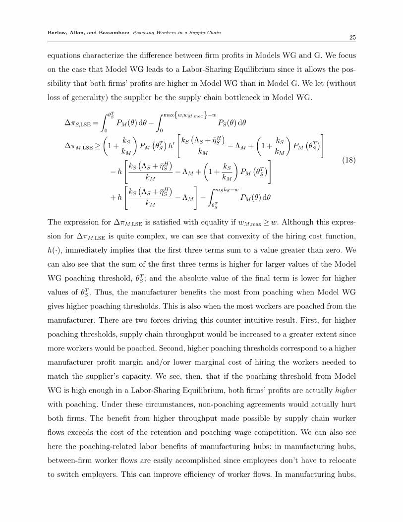
equations characterize the difference between firm profits in Models WG and G. We focus

on the case that Model WG leads to a Labor-Sharing Equilibrium since it allows the pos-

sibility that both firms’ profits are higher in Model WG than in Model G. We let (without

loss of generality) the supplier be the supply chain bottleneck in Model WG.

∆πS,LSE =

∫ θTS

0

PM(θ) dθ−∫ max{w,wM,max}−w

0

PS(θ) dθ

∆πM,LSE ≥(

1 +kSkM

)PM(θTS)h′

[kS(ΛS + η̄HS

)kM

−ΛM +

(1 +

kSkM

)PM(θTS)]

−h

[kS(ΛS + η̄HS

)kM

−ΛM +

(1 +

kSkM

)PM(θTS)]

+h

[kS(ΛS + η̄HS

)kM

−ΛM

]−∫ mSkS−w

θTS

PM(θ) dθ

(18)

The expression for ∆πM,LSE is satisfied with equality if wM,max ≥w. Although this expres-

sion for ∆πM,LSE is quite complex, we can see that convexity of the hiring cost function,

h(·), immediately implies that the first three terms sum to a value greater than zero. We

can also see that the sum of the first three terms is higher for larger values of the Model

WG poaching threshold, θTS ; and the absolute value of the final term is lower for higher

values of θTS . Thus, the manufacturer benefits the most from poaching when Model WG

gives higher poaching thresholds. This is also when the most workers are poached from the

manufacturer. There are two forces driving this counter-intuitive result. First, for higher

poaching thresholds, supply chain throughput would be increased to a greater extent since

more workers would be poached. Second, higher poaching thresholds correspond to a higher

manufacturer profit margin and/or lower marginal cost of hiring the workers needed to

match the supplier’s capacity. We see, then, that if the poaching threshold from Model

WG is high enough in a Labor-Sharing Equilibrium, both firms’ profits are actually higher

with poaching. Under these circumstances, non-poaching agreements would actually hurt

both firms. The benefit from higher throughput made possible by supply chain worker

flows exceeds the cost of the retention and poaching wage competition. We can also see

here the poaching-related labor benefits of manufacturing hubs: in manufacturing hubs,

between-firm worker flows are easily accomplished since employees don’t have to relocate

to switch employers. This can improve efficiency of worker flows. In manufacturing hubs,


then, the interaction between the flow of goods and the flow of workers can benefit all

supply chain members.

We see in (18) the reason for the poaching success in the shale oil and gas industry.

With the shale extraction firms poaching skilled labor, the downstream customers have

a relatively low marginal cost of double hiring. Furthermore, the customers experience a

large production payoff for allowing their workers to be poached. Thus, their maximum

equilibrium wages are low. This leads to a high poaching threshold. Both shale oil and its

customers benefit because poaching is available as a means to accomplish worker flows.

However, if Apple and members of its value chain were to allow poaching of developers

and managers, the marginal hiring costs would be high. Furthermore, the firms would

receive little benefit from allowing workers to be poached by value chain partners. Thus,

the maximum equilibrium wages are high and the poaching threshold is low. Apple and

its partners would thus be worse off without no-poaching agreements.

4.2. Comparative Statics

We now proceed to present comparative statics on the poaching threshold, θTi . With the

comparative statics results, we show how the worker flows depend on the model primitives.

If the poaching threshold increases in a Labor-Sharing Equilibrium, a weakly larger number

of workers flow to the bottleneck firm from its supply chain partner. However, increasing

the poaching threshold in a Labor-Hoarding Equilibrium leads to a weakly smaller number

of the bottleneck firm’s workers poached by its supply chain partner. We let firm i∈ {M,S}

be the supply chain bottleneck, and we let firm j be firm i’s supply chain partner.

Proposition 2 (Comparative Statics). In equilibria in which firm i∈ {M,S} is the

supply chain bottleneck (with supply chain partner j), an increase in kj (firm j’s individual

worker productivity) or pF (price of the final good) causes a weak increase in the poaching

threshold, θTi . Increasing production costs cM or cS results in a weakly decreasing poaching

threshold, θTi .

With workers who are individually more productive, firm j is able to achieve higher pro-

duction from retained and poached workers and higher production from hired workers.

Furthermore, the number of workers firm j must hire to match firm i’s production capacity

is reduced. Thus, firm j is more prone to allow its workers to be poached. In a manufac-

turing hub, then, we see that labor flows can distribute the benefits of enhanced worker


productivity even without knowledge spillover effects: the supply chain bottleneck retains

and poaches weakly more workers, experiences weakly higher production capacity and sup-

ply chain throughput, and earns weakly higher profits when firm j’s workers become more

productive.

The supply chain partners also share the benefits when the price of the final good

increases. If the manufacturer is the supply chain bottleneck, an increase in pF implies that

the manufacturer can afford to offer a higher poaching wage. Thus, throughput increases.

If the supplier is the bottleneck, then the manufacturer becomes more willing to allow its

workers to be poached so that it can capitalize on higher throughput.

Changes in production costs are also shared. Increasing production costs, cS or cM ,

decrease the firm margins. Labor sharing becomes less beneficial since the payoff for sharing

workers is reduced. Furthermore, with increased production costs, the bottleneck cannot

afford wages as high and thus cannot afford to poach as many workers.

4.3. Labor Market Competition

Thus far in our analysis, we have considered a single supplier and a single manufacturer.

Thus, the firms have not had to compete with other firms for workers, and the workers have

not had specific employment options outside the supply chain. Now we examine the impact

of additional labor market competition on our results. Specifically, we assume that a labor

market competitor, firm C, is also attempting to poach and retain workers. This labor

market competitor does not participate in the supply chain and only serves as a potential

source of workers to poach or a potential poacher. We let wC,max > w be the exogenous

maximum wage that the labor market competitor is willing to pay in the poaching and

retention stage. Without loss of generality, we let firm i represent the firm (either the

supplier or manufacturer) limiting supply chain throughput, and firm j represents firm i’s

supply chain partner.

Our first result relates to the presence of a labor market competitor that is more pro-

ductive than the supply chain bottleneck.

Proposition 3. The presence of a labor market competitor makes supply chain worker

flows impossible if:

1. wC,max >kimi,


2. there exists a wCj,max satisfying

wCj,max = h′

[ki[Λi−Pi (wC,max− kimi) + η̄Hi

]kj

−Λj +Pj(wC,max−wC

j,max

)]

such that wC,max > wCj,max, wC,max >

(1 + ki

kj

)wCj,max − kimj, and

ki[Λi−Pi (wC,max− kimi) + η̄Hi

]<kj

[Λj −Pj

(wC,max−wC

j,max

)+ η̄Hj

].

Supply chain throughput is reduced if such a labor market competitor is present.

The conditions in Proposition 3 guarantee: (i) the labor market competitor is willing to

offer wages higher than any wage offers from the manufacturer or supplier, and (ii) firm i

is indeed limiting supply chain throughput in equilibrium.

In these equilibria, both supply chain partners must pay high wages to retain workers,

and the poaching by the labor market competitor reduces supply chain throughput. Thus,

we see that the labor costs of being in a manufacturing hub with highly productive labor

market competitors have the potential to be far more substantial than simple costs of

wage competition. Highly productive labor market competition can hurt supply chain

throughput and eliminate worker flows between supply chain partners. This insight also

gives us some additional information regarding entry of a new labor market competitor. A

highly productive entrant can shut down supply chain labor sharing. In this case, poaching

would no longer serve as a means to increase supply chain bottleneck capacity.

We find, however, that if kimi > wC,max, then Labor-Sharing Equilibria may continue

to exist under conditions similar to those in the original model. Thus, the existence of

Labor-Sharing Equilibria and the subsequent results are robust to the presence of labor

market competition as long as the competitors are not more productive than the supply

chain bottleneck. However, labor market competition often leads to lower profits as the

firms must offer higher wages to ward off the competitor’s poaching attempts.

4.4. Model Robustness

We performed a number of tests on the model to ensure robustness. We briefly mention

robustness with respect to demand uncertainty. In our test, the manufacturer faces demand

uncertainty in a Newsvendor setting. We found that the results of the model continued with

minor discrepancy. The primary difference between our model and the model extension with

demand uncertainty comes as a result of decreasing returns to production associated with

the uncertain demand. Decreasing returns to production imply that the manufacturer’s


marginal payoff for hiring workers decreases, so if the manufacturer poaches and retains

more workers, its maximum optimal hiring level decreases. Because of this, the supplier may

be less willing to allow its workers to be poached since the supplier’s value of each additional

worker poached by the manufacturer is weakly decreasing. Despite the differences, however,

Labor-Sharing Equilibria continue to exist with uncertain demand.

5. Conclusion

In this paper, we’ve highlighted interesting results and insights stemming from the interac-

tion between the flow of goods and the flow of workers via poaching in a supply chain. We

have shown that it may be optimal to allow a less productive firm to poach workers from

members of its supply chain so that the supply chain throughput can be enhanced. In fact,

the more productive the workers employed by the supply chain partners and the greater

the partners’ profit margin, the greater the tendency for labor sharing. These insights run

counter to classical intuition from labor economics. Furthermore, labor sharing via poach-

ing actually provides a net benefit to all supply chain firms in the case that the marginal

revenues from increased throughput exceed both the marginal costs of hiring workers and

the higher wages that must be paid to poach and retain workers.

This insight provides an explanation for the differences in the response to poaching

observed between the shale industry and Apple. The customers of the shale oil and gas

industry get high payoffs from higher supplier poaching. And the marginal cost of “double

hiring” is relatively low for the skilled laborers poached by the shale oil extraction firms.

Thus, worker flows made available via poaching are able to increase throughput and the

resulting profits for all members of the supply chain. However, with Apple and its partners,

the marginal benefit of allowing an additional engineer or developer to be poached is low;

and the marginal hiring cost is high for these workers. Thus, poaching and retention wages

would be very high without no-poaching agreements. Since the higher wages and hiring

costs exceed the benefits of allowing engineers and developers to be poached, it becomes

desirable for Apple and its business partners to avoid poaching altogether by entering into

no-poaching agreements.

One of our primary results relates to the idea that poaching has the potential to impact

our views of supply chain capacity management. Traditionally, we think of the bottleneck

as the resource with the lowest capacity. In our model, the bottleneck firm is the supply


chain partner that is unwilling to further increase its capacity by hiring additional workers.

We have shown that the availability of poaching can change the identity of the bottle-

neck firm. Thus, consideration of worker flows accomplished via poaching can be critical

understanding supply chain bottleneck capacity management.

We also find that the presence of a highly productive labor market competitor shuts

down the possibility of labor sharing, decreases throughput, and decreases profits. However,

labor sharing between supply chain partners is robust to labor market competition if the

competitor has lower labor productivity than the supply chain bottleneck. The robustness

of labor sharing between members of a supply chain even in the presence of outside labor

competition highlights the poaching-induced labor benefits of operating in a manufacturing

hub. Close proximity to other members of a supply chain may help provide for efficient

worker flows without excessive poaching/retention wages.

References

Aksin, Zeynep, Mor Armony, Vijay Mehrotra. 2007. The modern call center: A multi-disciplinary perspective

on operations management research. Production and Operations Management 16(6) 665–688.

Becker, Gary S. 1962. Investment in human capital: A theoretical analysis. Journal of Political Economy

70 pp. 9–49.

Blatter, Marc, Samuel Muehlemann, Samuel Schenker. 2012. The costs of hiring skilled workers. European

Economic Review 56(1) 20–35.

Boston Consulting Group. 2013. Cheap natural gas could save u.s. households as much as $1,200 a year by

2020. URL http://www.bcg.com/media/pressreleasedetails.aspx?id=tcm:12-151944.

Campbell, Mikey. 2014. Lawsuit claims steve jobs, senior apple directors hurt com-

pany with anti-poaching row. URL http://appleinsider.com/articles/14/08/15/

lawsuit-claims-steve-jobs-senior-apple-directors-hurt-company-with-anti-poaching-row.

Combes, Pierre-Philippe, Gilles Duranton. 2006. Labour pooling, labour poaching, and spatial clustering.

Regional Science and Urban Economics 36(1) 1–28.

Daskin, Mark S, Lawrence V Snyder, Rosemary T Berger. 2005. Facility location in supply chain design.

Logistics systems: Design and optimization. Springer, 39–65.

Davis, Jess. 2013. Eagle ford worker shortage prompts spike in noncompetes. URL http://www.law360.

com/articles/430424/eagle-ford-worker-shortage-prompts-spike-in-noncompetes.

Demirbag, Mehmet, Kamel Mellahi, Sunil Sahadev, Joel Elliston. 2012. Employee service abandonment in

offshore operations: A case study of a us multinational in india. Journal of World Business 47(2)

178–185.

http://www.bcg.com/media/pressreleasedetails.aspx?id=tcm:12-151944

http://appleinsider.com/articles/14/08/15/lawsuit-claims-steve-jobs-senior-apple-directors-hurt-company-with-anti-poaching-row

http://appleinsider.com/articles/14/08/15/lawsuit-claims-steve-jobs-senior-apple-directors-hurt-company-with-anti-poaching-row

http://www.law360.com/articles/430424/eagle-ford-worker-shortage-prompts-spike-in-noncompetes

http://www.law360.com/articles/430424/eagle-ford-worker-shortage-prompts-spike-in-noncompetes


Ellison, Glenn, Edward L Glaeser. 1997. Geographic concentration in u.s. manufacturing industries: A

dartboard approach. Journal of Political Economy 105(5) 889–927.

Fallick, Bruce, Charles A Fleischman. 2001. The importance of employer-to-employer flows in the US labor

market , vol. 1. Divisions of Research & Statistics and Monetary Affairs, Federal Reserve Board.

Gans, Noah, Ger Koole, Avishai Mandelbaum. 2003. Telephone call centers: Tutorial, review, and research

prospects. Manufacturing & Service Operations Management 5(2) 79–141.

Harrigan, James, Anthony J Venables. 2006. Timeliness and agglomeration. Journal of Urban Economics

59(2) 300–316.

Jones, Garett, Daniel M Rothschild, Mercatus Center. 2011. Did Stimulus Dollars Hire the Unemployed?:

Answers to Questions about the American Recovery and Reinvestment Act . Mercatus Center, George

Mason University.

Katz, Eliakim, Adrian Ziderman. 1990. Investment in general training: The role of information and labour

mobility. The Economic Journal 100 pp. 1147–1158.

Klier, Thomas H. 1999. Agglomeration in the us auto supplier industry. ECONOMIC PERSPECTIVES-

FEDERAL RESERVE BANK OF CHICAGO 23 18–34.

Krugman, Paul R. 1991. Geography and trade. MIT press.

Marx, Matt, Deborah Strumsky, Lee Fleming. 2009. Mobility, skills, and the michigan non-compete experi-

ment. Management Science 55(6) 875–889.

Milner, Joseph M, Edieal J Pinker. 2001. Contingent labor contracting under demand and supply uncertainty.

Management Science 47(8) 1046–1062.

Olson, Bradley, Edward Klump, Jack Kaskey. 2013. Dearth of skilled workers imper-

ils $100 billion projects. URL http://www.bloomberg.com/news/2013-03-07/

dearth-of-skilled-workers-imperils-100-billion-projects.html.

PayScale Inc. 2014. 2013-2014 payscale college salary report. URL http://www.payscale.com/

college-salary-report-2014.

Rosenthal, Stuart S, William C Strange. 2004. Evidence on the nature and sources of agglomeration

economies. Handbook of regional and urban economics 4 2119–2171.

Sargent, Thomas J. 1978. Estimation of dynamic labor demand schedules under rational expectations. The

Journal of Political Economy 1009–1044.

Sarkis, Joseph. 2001. Manufacturing’s role in corporate environmental sustainability: Concerns for the new

millennium. International Journal of Operations & Production Management 21(5) 666–686.

Schonberger, Richard. 1982. Japanese manufacturing techniques: Nine hidden lessons in simplicity . Simon

and Schuster.

Serafinelli, Michel. 2013. Good firms, worker flows and productivity. Working Paper.

http://www.bloomberg.com/news/2013-03-07/dearth-of-skilled-workers-imperils-100-billion-projects.html

http://www.bloomberg.com/news/2013-03-07/dearth-of-skilled-workers-imperils-100-billion-projects.html

http://www.payscale.com/college-salary-report-2014

http://www.payscale.com/college-salary-report-2014


Smith, Donald F, Richard Florida. 1994. Agglomeration and industrial location: An econometric analysis

of japanese-affiliated manufacturing establishments in automotive-related industries. Journal of Urban

Economics 36(1) 23–41.

Sorkin, Andrew Ross. 2014. Tech firms may find no-poaching pacts costly. URL http:

//dealbook.nytimes.com/2014/04/07/tech-firms-may-find-no-poaching-pacts-costly/?_

php=true&_type=blogs&_php=true&_type=blogs&_r=1.

Tambe, Prasanna, Lorin M Hitt. 2014. Job hopping, information technology spillovers, and productivity

growth. Management Science 60(2) 338–355.

Appendix. Proofs

We omit the proof of Proposition 3 since it is so similar to the proofs of Lemma 3 and Proposition 1.

Proof of Lemma 1: This proof follows by solving the supplier’s problem in (5) and using the supplier’s

optimum strategy to solve the manufacturer’s problem in (4). We use the two optimum strategies together

to determine the equilibrium outcome in the sub-game beginning at the start of Stage 2 in state N .

We begin by noting that the supplier has no incentive in (5) to have qS > qM . Such production levels incur

the production cost but don’t add to revenue. Thus, an equivalent optimization problem is:

VS (N,qM) = maxqS ,ηS

mSqS −h(ηHS )

subject to: qS ≥ 0; qS ≤ kS (NS + ηHS ); qS ≤ qM ; ηHS ≥ 0.

The Lagrangian for this problem (with all λ representing the multipliers for the inequality constraints) is:

L=mSqS −h(ηHS ) +λqqS +λK[kS (NS + ηHS )− qS

]+λM (qM − qS) +ληη

HS

For first-order conditions, then, we get:

[qS] : 0 =mS +λ∗q −λ∗K −λ∗M

[ηHS ] : 0 = λ∗η +λ∗KkS −h′(ηH ∗S (N,qM)

)Since mS > 0, λ∗q = 0; so it’s optimal for the supplier to increase capacity until its capacity constraint is

binding, until the manufacturer’s order constraint is binding, or until both are binding. If the manufacturer’s

order constraint is binding but the capacity constraint is not, q∗S (N,qM) = qM and ηH∗

S = 0: if the supplier

can completely fulfill the manufacturer’s order without being capacity-constrained, it will perfectly satisfy

the order and not hire any additional workers. If the capacity constraint is binding but the manufacturer’s

order constraint is not, the supplier hires up to the point that h′ (ηHS ) = kSmS. This level of hiring represents

the maximum optimal hiring level, η̄HS . The supplier produces at the level corresponding to its capacity,

q∗S (N,qM) = kS (NS + η̄HS ). In the final case, both the capacity constraint and the manufacturer’s order

constraint are binding. In other words, the supplier hires enough workers so that its capacity is equal

to the manufacturer’s order quantity. Thus, in this case, the supplier must hire ηHS∗ (N,qM) = qM

kS− NS

workers to satisfy the manufacturer’s order, and the order quantity corresponds to the manufacturer’s order,

q∗S (N,qM) = qM . Thus, we get that the supplier’s optimal strategy is:

q∗S (N,qM) = min{qM , kS

(NS + η̄HS

)}ηH ∗S (N,qM) =

[min

{η̄HS ,

qMkS−NS

}]+

http://dealbook.nytimes.com/2014/04/07/tech-firms-may-find-no-poaching-pacts-costly/?_php=true&_type=blogs&_php=true&_type=blogs&_r=1




Now we turn to the manufacturer’s Stage 2 optimum strategy. We begin by substituting the supplier’s

optimal Stage 3 strategy into (4) to get:

VM (N) = maxqM ,ηM

mM min{qM , kS

(NS + η̄HS

)}−h(ηHM)

subject to: qM ≥ 0; qM ≤ kM(NM + ηHM); ηHM ≥ 0.

Since no benefit is provided by ordering more than kS (NS + η̄HS ), we can re-write the problem again as:

VM (N) = maxqM ,ηM

mMqM −h(ηHM)

subject to: qM ≥ 0; qM ≤ kM(NM + ηHM); qM ≤ kS(NS + η̄HS

); ηHM ≥ 0.

This problem is identical to the supplier’s except that the supplier’s production is bounded above by qM ,

whereas the manufacturer’s is bounded above by kS (NS + η̄HS ). Thus, using the solution to the supplier’s

problem, we get that the manufacturer’s optimal strategy is:

q∗M (N) = min{kM(NM + η̄HM

), kS

(NS + η̄HS

)}ηH ∗M (N) =

[min

{η̄HM ,

kS (NS + η̄HS )

kM−NM

}]+

Combining the optimum manufacturer and supplier strategies in Stages 2 and 3, we get (6) as the equilibrium

outcome for the sub-game beginning in Stage 2 in state N .

�

Proof of Lemma 2: Consider firm i∈ {M,S} with supply chain partner j. We look for equilibrium wage

offers; so each firm’s wage offers must be best responses to the supply chain partner’s wage offers. We assume

firm j offers poaching and retention wages according to (10) and (11), respectively. We show that firm i’s

best response is to offer poaching and retention wages according to (10) and (11), respectively. To do this, we

note that firm i would not be willing to pay more than w(eq)i,max (the marginal benefit of an additional worker)

in equilibrium to poach or retain a worker. We further recall that the equations for successful poaching and

retention are given in (1) and (2), respectively.

We first focus on firm i’s optimal poaching wages. For all of firm j’s workers for whom w(eq)i,max >

max{wR∗j (θ),w

}+ θ, it’s optimal for firm i to offer a poaching wage equal to wθi = max

{wR∗j (θ),w

}+ θ,

which is the minimum wage that must be offered to successfully poach a worker of type θ from firm j. With

this wage offer, all of firm j’s workers for whom w(eq)i,max >max

{wR∗j (θ),w

}+ θ are successfully poached by

firm i. For all of firm j’s workers for which w(eq)i,max ≤max

{wR∗j (θ),w

}+ θ, it’s optimal for firm i to offer

a poaching wage equal to wθi = w(eq)i,max. This amount represents the maximum firm i would be willing to

pay. However, since these workers are not successfully poached, firm i does not actually have to pay this

amount. Substituting in wR∗j (θ), we see that all of firm j’s workers of type θ≤w(eq)i,max−max

{w,w

(eq)j,max

}are

successfully poached by firm i, and they must be offered max{w,w

(eq)j,max

}+ θ to entice them to leave. The

remaining workers employed at firm j are not affordable by firm i and are not poached. Thus, it is optimal

to offer them w(eq)i,max. Thus, we find that wP ∗i (θ) = min

{w

(eq)i,max,max

{w,w

(eq)j,max

}+ θ}

.

Now we turn to firm i’s optimal retention wages. The marginal benefit of retaining a worker depends on

whether the worker could be poached by the supply chain partner. If the worker could not be poached, then

the marginal benefit of retaining the worker depends only on either firm i’s labor productivity or its marginal


hiring cost (depending on whether firm i is the bottleneck or not, respectively), which are both greater than

the reservation wage, w. Since the worker could not be poached by the supply chain partner, however, firm

i needs only offer w to successfully retain the worker. Given firm j’s poaching wage strategy, this holds for

all workers of type θ≥max{w

(eq)j,max,w

}−w.

If the worker could be poached, then firm i must account for the fact that an additional worker retained

translates into one less worker firm j could poach. This effect is captured in w(eq)i,max. Thus, for workers of

type θ ≤max{w

(eq)j,max,w

}− w(eq)

i,max, firm i would have to offer more than max{w

(eq)j,max,w

}to successfully

retain them. However, if w(eq)j,max >w

(eq)i,max, then firm i cannot afford to offer enough to retain the workers; so it

optimally offers the most it can afford, w(eq)i,max, to retain them. For worker types max

{w

(eq)j,max,w

}−w(eq)

i,max <

θ <max{w

(eq)j,max,w

}−w, firm i can retain them with an offer of max

{w,w

(eq)j,max− θ

}. Since, for these workers,

w(eq)i,max >max

{w,w

(eq)j,max− θ

}, firm i optimally offers max

{w,w

(eq)j,max− θ

}and successfully retains them. All

of the cases for optimal retention, then, can be written by wR∗i (θ) = max{w,min

{w

(eq)j,max− θ,w

(eq)i,max

}}.

Thus, the poaching and retention wages in Lemma 2 are best-responses to firm j’s strategy when firm j

uses these strategies. Thus, these are equilibrium poaching and retention wage offers.

�

Proof of Lemma 3: In equilibria in which the supplier is the supply chain bottleneck and the manufacturer

optimally hires workers in the second stage, the manufacturer’s equilibrium maximum optimal wage is given

by (9) with (14) substituted in for NS and NM . Substituting the resulting expressions into (12) gives the

result.

�

Proof of Theorem 1: Here, we prove the general version of Theorem 1 that allows for either firm to be

limiting supply chain throughput.

We first assume that an LSE exists in which the firm i is the bottleneck and firm j is firm i’s supply

chain partner. By the definition of an LSE, the manufacturer must hire a strictly positive number of workers

to match, so µj(θTi ) > 0. This also implies satisfaction of the second condition by Proposition 3. The fact

that firm i is the bottleneck in equilibrium implies that firm i’s maximum optimal production capacity at

poaching threshold θTi is less than firm j’s maximum optimal production capacity at the same poaching

threshold. Thus, the third condition is satisfied.

Now we assume that there exists a θTi > 0 that satisfies the three conditions of Theorem 1. Existence

of such a poaching threshold implies that µM(θTS ) > 0, so the manufacturer must hire a strictly positive

number of workers to match the supplier’s maximum optimal production capacity. Satisfaction of the second

condition implies that the θTi corresponds to an equilibrium poaching threshold. And the third condition

implies that firm i is the supply chain bottleneck. Thus, this value of θTi corresponds to an LSE since the

equilibrium outcome it fits the definition.

Now we turn to the more involved portion of the proof: showing that if there exists a θTi > 0 that satisfies

all of the conditions of Theorem 1, the game has a unique equilibrium outcome. We begin by assuming

existence of a θTi > 0 that satisfies all three conditions of Theorem 1. We first show that existence of such a θTi

precludes existence of any other equilibrium outcome with firm i as the supply chain bottleneck. To do this,


we focus on the second condition of Theorem 1. The left-hand side is continuous and strictly increasing in

θTi . The right-hand side is weakly decreasing in θTi since µj(·) is weakly increasing h′(·) is strictly increasing.

Thus, since the left-hand side is strictly increasing and the right-hand side is weakly decreasing in θTi , there

can exist at most one solution to the second condition. Thus, there are no other equilibria in which firm i is

the bottleneck.

Now we show that there are no equilibria in which firm j is the supply chain bottleneck. We first

show that there are no equilibrium θTj ≥ 0. Existence of such an equilibrium θTj would imply that

kj[Λj + η̄Hj +Pi

(θTj)]≤ ki

[Λi + η̄Hi −Pi

(θTj)]

, which implies that kj(Λj + η̄Hj

)≤ ki (Λi + η̄Hi ) since P (·)≥ 0.

However, since there exists a θTi > 0 satisfying the third condition of Theorem 1, we have for this θTi that

ki [Λi + η̄Hi +Pj (θTi )] < kj[Λj + η̄Hj −Pj (θTi )

], so that ki (Λi + η̄Hi ) < kj

(Λj + η̄Hj

), a contradiction. Thus,

there are no equilibria in which firm j is the bottleneck and θTj ≥ 0.

Finally, we show that no equilibria exist with θTj < 0 given that there exists a θTi > 0 that satisfies the

conditions of Theorem 1. To prove this by contradiction, we assume that there exists an equilibrium θTj < 0

that satisfies:

1. θTj = kjmj + kjmi−(

1 +kj

ki

)h′[kj[Λj+η̄Hj −Pj(−θTj )]−ki[Λi+η̄

Hi +Pj(−θTj )]

ki+ η̄Hi

]2. kj

[Λj + η̄Hj −Pj

(−θTj

)]≤ ki

[Λi + η̄Hi +Pj

(−θTj

)].

Consider the set of all θj ≤ 0 that satisfy the second condition. That is, let Θj ={θj < 0 : kj

[Λj + η̄Hj −Pj (−θj)

]≤ ki [Λi + η̄Hi +Pj (−θj)]

}. If the set Θj is empty, then the proof is done:

there are no θj ≤ 0 that satisfy the second condition, so there are no equilibria with θTj < 0. So let’s assume

that the set Θj is non-empty. Let θ̄j = sup Θj . Since Pj(·) is a positive weakly increasing function, all

θ̄j satisfy kj[Λj + η̄Hj −Pj

(−θ̄j

)]= ki

[Λi + η̄Hi +Pj

(−θ̄j

)]. We see, then, that our definition of Θj and

the third condition of Theorem 1 imply that 0 < θTi < −θj for any θj ∈ Θj . Specifically, these imply that

0< θTi <−θ̄j . We substitute our definition of θ̄j into the right-hand side of the first equilibrium condition

and get:

kjmj + kjmi−(

1 +kjki

)h′

[kj[Λj + η̄Hj −Pj

(−θ̄j

)]− ki

[Λi + η̄Hi +Pj

(−θ̄j

)]ki

+ η̄Hi

]

= kjmj + kjmi−(

1 +kjki

)h′(η̄Hi)

= kjmj + kjmi−(

1 +kjki

)kimi

= kjmj + kjmi− kimi− kjmi

= kjmj − kimi,

where the second line follows because θ̄j satisfies kj[Λj + η̄Hj −Pj

(−θ̄j

)]= ki

[Λi + η̄Hi +Pj

(−θ̄j

)]and the

third line follows because of the definition of η̄Hi . Since the right-hand side of the first equilibrium condition

above is weakly decreasing in θTj and the left-hand side is strictly increasing, we get that any θTj < 0 that

satisfies both equilibrium conditions above also satisfies kjmj−kimi ≤ θTj ≤ θ̄j . This, in turn, implies that it

also satisfies kimi−kjmj ≥−θTj ≥−θ̄j . Now we turn back to examining the θTi > 0 satisfying the equilibrium

conditions of Theorem 1. The third equilibrium condition of Theorem 1 implies that the argument of h′(·)


in the second equilibrium condition is less than η̄Hj . Thus, the strict convexity of h(·) from Assumption 1(a)

implies that:

h′

[ki [Λi + η̄Hi +Pj (θTi )]− kj

[Λj + η̄Hj −Pj (θTi )

]kj

+ η̄Hj

]<h′

(η̄Hj)

= kjmj .

Thus, we get that:(1 +

kikj

)h′



]kj

+ η̄Hj

]− kimj <

(1 +

kikj

)kjmj − kimj

= kjmj .

By Assumptions 1(b) and 1(c), we also have that kjmj >w. Thus, we get that:

max

{w,

(1 +

kikj

)h′



]kj

+ η̄Hj

]− kimj

}<kjmj .

Finally, we get that the right-hand side of the second condition of Theorem 1 satisfies:

kimi−max

{w,

(1 +

kikj

)h′



]kj

+ η̄Hj

]− kimj

}>kimi− kjmj .

Thus, we get that the right-hand side of the first equilibrium condition of Theorem 1 is always greater than

kimi − kjmj for all θTi that satisfy the third equilibrium condition. Since the right-hand side of the second

condition of Theorem 1 is weakly decreasing in θTi and the left-hand side is strictly increasing in θTi , we

get that any θTi > 0 that satisfies all equilibrium conditions of Theorem 1 also satisfies θTi > kimi − kjmj .

However, from our analysis of the θTj < 0 that satisfies the equilibrium conditions above for a Labor-Hoarding

Equilibrium with firm j as the bottleneck, we found that kimi−kjmj ≥−θTj ≥−θ̄j . We also found that any

θTi > 0 that satisfies the second equilibrium condition of Theorem 1 also satisfies 0< θTi <−θ̄j . Combining

these inequalities, we get that:

kimi− kjmj ≥−θTj ≥−θ̄j > θTi >kimi− kjmj ,

a contradiction. Thus, existence of a θTi > 0 that satisfies the equilibrium conditions of Theorem 1 precludes

existence of a θTj < 0 that satisfies the equilibrium conditions above for a Labor-Hoarding Equilibrium with

firm j as the bottleneck.

Thus, we have ruled out equilibria with θTj < 0 that satisfy the first Labor-Hoarding Equilibrium condition.

However, we must also rule out equilibria that may have θTj < 0 with a discontinuous jump in the right-

hand side of the first Labor-Hoarding Equilibrium condition at θTj . Such an equilibrium would require that

µi(−θTj

)= 0 and

θTj >kjmj + kjmi−(

1 +kjki

)h′(0) = kjmj −h′(0) +

kjki

[kimi−h′(0)]> 0,

where the final inequality follows because of Assumption 1(c). Thus, equilibria in which there exists a

discontinuity at the equilibrium poaching threshold cannot exist for θTj ≤ 0. Thus, we have now ruled out

existence of any equilibria with θTj < 0.

Thus, we have shown that existence of a θTi > 0 that satisfies the conditions of Theorem 1 precludes exis-

tence of any other equilibrium θTi , any equilibrium θTj ≥ 0, or any equilibrium θTj < 0. Since any equilibrium

outcome must fit into one of these bins, it follows that any θTi > 0 that satisfies the three conditions of

Theorem 1 represents the unique equilibrium outcome.


�

Proof of Corollary 1: We begin by assuming existence of a Labor-Hoarding Equilibrium in which firm i

is the bottleneck. By the definition, firm j is the poacher and thus offers a higher wage. This implies that

at this equilibrium, θTi < 0. As we showed in the proof of Theorem 1, there cannot exist any θTi < 0 in

which (16) is not satisfied with equality in equilibrium. Since kimi > w by Assumption 1(b) and (c), and

firm j’s equilibrium maximum wage offer is higher than firm i’s (which is equal to kimi), we get that firm

j’s maximum wage offer is greater than w. Thus, we get that (16) reduces to the first condition and must

be satisfied with equality. Since firm i is the bottleneck, its maximum optimal capacity at the equilibrium

poaching threshold must be lower. Thus, the second condition must be satisfied.

Now we assume that there exists a θTi < 0 that satisfies the two conditions of Corollary 1. Since θTi < 0,

firm j is willing to offer higher wages at this poaching threshold and is thus the poacher. Also, since the

second condition is satisfied, firm i is the supply chain bottleneck at this poaching threshold. Finally, since

the first condition is satisfied, this poaching threshold satisfies the equilibrium requirement given that firm i

is the supply chain bottleneck at this poaching threshold. Thus, this poaching threshold corresponds to an

equilibrium in which firm i is the bottleneck but firm j is poaching workers from firm i. In other words, it

corresponds to a Labor-Hoarding Equilibrium.

For uniqueness, we begin by following the proof of Theorem 1 and notice since all equilibria with θTi < 0

must satisfy (16) with equality, the left-hand side of (16) is strictly increasing, and the right-hand side of

(16) is weakly decreasing and continuous for all θ ≥ θTi satisfying the first condition, it must be the only

equilibrium with firm i as the bottleneck. Furthermore, as we showed in the proof of Theorem 1, existence

of a LHE firm firm i as the bottleneck rules out existence of any LSE with firm j as the bottleneck. Finally,

we showed in the proof of Theorem 1 that in any LHE with firm j as the bottleneck, kimi > kjmj . Since

a symmetric result holds in any LHE in which firm i is the bottleneck, it must be that kjmj > kimi, so no

LHE can exist with firm j is the bottleneck since it would imply that kimi > kjmj > kimi, a contradiction.

Thus, we get a similar uniqueness result and kjmj >kimi.

�

Proof of Theorem 2: We begin by assuming that the two conditions of Theorem 2 are satisfied. Since

ki (Λi + η̄Hi ) > kjΛj , µj(θ) > 0. Thus, the right-hand side of (16) is well-defined, continuous, and weakly

decreasing for all θ≥ 0. Since Qi > 0 and kimi >w, the right-hand side of (16) is positive for θTi = 0. Thus,

since the left-hand side is continuous and strictly increasing from zero and the right-hand side is positive for

θTi = 0, continuous, and weakly decreasing from Qi, we get that the fixed point of (16) exists and is strictly

greater than zero and weakly less than Qi. Thus, since Pj(·) is weakly increasing, Pj (Qi) > Pj (θTi ). This

implies, then, that ki [Λi + η̄Hi +Pj (θTi )] < kj[Λj + η̄Hj −Pj (θTi )

]. Thus, there exists a θTi > 0 that satisfies

all conditions of Theorem 1 and thus corresponds to a Labor-Sharing Equilibrium.

�

Proof of Proposition 1: (a) WLOG, let firm i be the supply chain bottleneck. In an LSE, then, the

equilibrium poaching threshold, θTi , satisfies ki [Λi + η̄Hi +Pj (θTi )]< kj[Λj + η̄Hj −Pj (θTi )

]. The throughput

in Model WG is ki [Λi + η̄Hi +Pj (θTi )]. Since Pj(·) ≥ 0, the previous inequality implies that ki (Λi + η̄Hi ) <


kj(Λj + η̄Hj

), which implies that firm i is the bottleneck firm in Model G and supply chain throughput is

ki (Λi + η̄Hi ). Thus, throughput is weakly higher in Model WG.

(b) WLOG, let firm i be the supply chain bottleneck in both Models WG and G. Throughput in Model

WG in an LHE is given by ki [Λi + η̄Hi −Pi (−θTi )], and throughput in Model G is given by ki (Λi + η̄Hi ).

Thus, throughput is lower in Model WG than in Model G.

(c) WLOG, let firm j be the bottleneck in Model G. Thus, kj(Λj + η̄Hj

)<ki (Λi + η̄Hi ). We let

Θi ={θ < 0 : (ki + kj) Pi(−θ)>ki

(Λi + η̄Hi

)− kj

(Λj + η̄Hj

)}and θ̄i = sup Θi. Here, the set Θi represents the set of all poaching thresholds that would see firm i as the

bottleneck in Model WG. If kiη̄Hi <kj

(Λi + Λj + η̄Hj

), then the set Θi is non-empty since Pi(·)≤Λi. We also

see that, based on the definition of θ̄i,

kikj

[Λi + η̄Hi −Pi

(−θ̄i)]−Λj −Pi

(−θ̄i)> 0

since it is either equal to η̄Hj or ki (Λi + η̄Hi )− kjΛj , both of which are strictly positive. Thus, if

θ̄i >kimi + kimj −(

1 +kikj

)h′(kikj

[Λi + η̄Hi −Pi

(−θ̄i)]−Λj −Pi

(−θ̄i))

,

then the right-hand side of (16) is less than the left-hand side at θ̄i. Furthermore, if there exists a worker

type, θ0 such thatkikj

[Λi + η̄Hi −Pi (−θ0)

]−Λj −Pi (−θj) = 0,

then we know (from the proof of Theorem 1) that the right-hand side (16) is greater than zero at θ0.

Furthermore, since Pi(·) is weakly increasing, θ0 < θ̄i. We also see that the right-hand side of (16) is continuous

for all possible poaching thresholds between θ0 and θ̄i. If no θ0 exists, then the right-hand side of (16) is

continuous for all possible poaching thresholds no greater than θ̄i. Thus, since the right-hand side of (16)

is less than the left-hand side at θ̄i and is continuous and weakly decreasing, it intersects the left-hand side

for some θTi < θ̄i. Thus, the conditions of Corollary 1 are satisfied, and the equilibrium poaching threshold

corresponds to a Labor-Hoarding Equilibrium with firm i as the bottleneck.

�

Proof of Proposition 2: We begin with equilibrium poaching thresholds in which µj (θTi ) = 0 so that (16)

is satisfied with equality. Then we turn to the case in which µj (θTi ) = 0.

In equilibria in which (16) is satisfied with equality, we show the impact on the poaching threshold by

showing the impact on the right-hand side of (16). If a change increases the right-hand side for all θ such

that µj(θ)> 0, then it weakly increases the equilibrium poaching threshold since the new equilibrium still

represents the intersection between the right- and left-hand sides of (16) (for infinitesimal changes). An

increase in kj strictly decreases µj(θ) for all θ, causing a strict decrease of h′(·) for all θ. Thus, the change

weakly increases the right-hand side of (16) for all θ and thus weakly increases the poaching threshold.

It’s possible, however, than an increase in kj could force θTi to increase to the point that µj(θTi ) = 0. The

transition between regimes occur in a continuous manner at any point at which µj (θTi ) = 0 and

θTi = kimi−max

{w,

(1 +

kikj

)h′(0)− kimj

}.


We define θ0 = {θ : µj(θ) = 0}. Using (15), we find that Pj (θ0) is strictly increasing in kj ; so we find that the

equilibrium poaching threshold is always weakly increasing accompanying an increase in kj .

Now we turn to the comparative statics on pF . An increase in pF strictly (weakly) increases the right-

hand side of (16) if the manufacturer (supplier) is the bottleneck. Thus, in equilibria with (16) holding with

equality, increasing pF at least weakly increases the poaching threshold. In equilibria that don’t see (16)

holding with equality, increasing pF has no effect until equilibria are reached in which (16) holds again with

equality. Thus, increasing pF causes a weak increase in the poaching threshold. The proof showing the impact

of a change in production costs is essentially identical to the proof for the impact of a change in pF , so we

omit them.

�

Documents

Poaching Workers in a Supply Chain: Enemy from Within? · Electronic copy available at : http ://ssrn.com /abstract = 2560084 Poaching Workers in a Supply Chain: Enemy from Within?