Embed Size (px)
Citation preview

Climate Change Adaptation
Options Assessment
Developing flexible adaptation pathways for the Peron-
Naturaliste Coastal Region of Western Australia
Prepared for the Peron-Naturaliste Partnership
September 2012

Reliance and Disclaimer
The professional analysis and advice in this report has been prepared by ACIL Tasman for the exclusive use of the
party or parties to whom it is addressed (the addressee) and for the purposes specified in it. This report is supplied
in good faith and reflects the knowledge, expertise and experience of the consultants involved. ACIL Tasman
accepts no responsibility whatsoever for any loss occasioned by any person acting or refraining from action as a
result of reliance on the report, other than the addressee.
In conducting the analysis in this report ACIL Tasman has endeavoured to use what it considers is the best
information available at the date of publication, including information supplied by the addressee. Unless stated
otherwise, ACIL Tasman does not warrant the accuracy of any forecast or prediction in the report. Although ACIL
Tasman exercises reasonable care when making forecasts or predictions, factors in the process, such as future market
behaviour, are inherently uncertain and cannot be forecast or predicted reliably.
ACIL Tasman shall not be liable in respect of any claim arising out of the failure of a client investment to perform to
the advantage of the client or to the advantage of the client to the degree suggested or assumed in any advice or
forecast given by ACIL Tasman.
ACIL Tasman Pty Ltd
ABN 68 102 652 148
Internet www.aciltasman.com.au
Melbourne (Head Office) Level 4, 114 William Street Melbourne VIC 3000
Telephone (+61 3) 9604 4400 Facsimile (+61 3) 9604 4455 Email [email protected]
Brisbane Level 15, 127 Creek Street
Brisbane QLD 4000 GPO Box 32
Brisbane QLD 4001
Telephone (+61 7) 3009 8700 Facsimile (+61 7) 3009 8799
Email [email protected]
Canberra Level 2, 33 Ainslie Place Canberra City ACT 2600
GPO Box 1322 Canberra ACT 2601
Telephone (+61 2) 6103 8200 Facsimile (+61 2) 6103 8233 Email [email protected]
Perth Centa Building C2, 118 Railway Street
West Perth WA 6005
Telephone (+61 8) 9449 9600 Facsimile (+61 8) 9322 3955
Email [email protected]
Sydney Level 20, Tower 2 Darling Park 201 Sussex Street
Sydney NSW 2000 GPO Box 4670
Sydney NSW 2001
Telephone (+61 2) 9389 7842 Facsimile (+61 2) 8080 8142
Email [email protected]
For information on this report
Please contact:
Nick Wills-Johnson
Telephone (08) 9449 9616 Mobile 0404 665 219 Email [email protected]
Contributing team members
David Campbell Nick Wills-Johnson Tess Metcalf Matt Eliot (Damara WA) Simon Sagerer Glenn McCormack
(Damara WA) John Söderbaum

Climate Change Adaptation Options Assessment
ii
Contents
Executive summary v
1 Introduction 1
2 Economic Valuation of Climate Change Adaptation Measures 3
2.1 Concepts of value 6
2.2 Economic valuation techniques 10
2.3 Issues with economic valuation 24
3 The PNP Context 34
3.1 Description of the study area 34
3.2 Description of the impacts 46
4 Region-Wide Analysis 47
4.1 Calculating value at risk 47
4.2 Calculating the cost of each option 57
4.3 Results of analysis 61
5 Case Study Analysis 67
5.1 Differences from Chapter Four 68
5.2 Case Study One: Mandurah Estuary Mouth 78
5.3 Case Study Two: Siesta Park-Marybrook 94
5.4 Case Study Three: Peppermint Grove Beach 101
5.5 Case Study Four: Eaton-Collie River 108
5.6 Lessons learned from case studies 115
6 Conclusions and Steps Forward 120
7 Bibliography 125
Appendix A Cost of Insurance and Climate Change 132
Appendix B Discounting for Multi-Generational Projects 142
Appendix C Confidence in Cost Estimates 148
List of boxes
Box 1 Value at risk 10
Box 2 Decision relevant framework 24
Box 3 Planning and market responses to climate change 60
Box 4 Model simplifications 76
Box 5 Flood gates 92
Box 6 The decision tool and counter-intuitive results 107

Climate Change Adaptation Options Assessment
iii
Box A1 Suncorp’s response to recent flooding events in Queensland 140
List of figures
Figure 1 Measures of value 8
Figure 2 Peron Naturalist Partnership study region 34
Figure 3 Different discount rates sensitivity analysis 65
Figure 4 Illustration of the house-by-house problem 68
Figure 5 Mandurah case study areas 80
Figure 6 Mandurah northern beaches sub area groynes options – histograms of optimal timing 88
Figure 7 Mandurah Ocean Marina optimal protection times 89
Figure 8 Annual cost of sand replenishment – Sub Area 1 93
Figure 9 Siesta Park/ Marybrook case study sub-areas 96
Figure 10 Peppermint Grove beach case study areas 103
Figure 11 Optimal timing distribution for Options 5, 6 and 7 – Peppermint Grove Beach 106
Figure 12 Eaton-Australind case study sub-areas 110
Figure A1 Ratio of global weather-related property losses to total property/casualty premiums 135
Figure A2 Percentage change in US home insurance premiums between 2001 and 2006 136
Figure A3 Some NFIP statistics 138
List of tables
Table 1 Length of roads at risk (meters) 35
Table 2 The length of railway at risk (meters) 36
Table 3 Length of water mains at risk (meters) 36
Table 4 Length of sewerage lines at risk (meters) 37
Table 5 Length of electricity lines at risk (meters) 37
Table 6 Length of gas main at risk (meters) 37
Table 7 Area of community infrastructure at risk (meters squared) 38
Table 8 Area of residential land at risk (meters squared) 39
Table 9 Area of commercial land at risk (meters squared) 39
Table 10 Area of development land at risk (meters squared) 40
Table 11 Area of rural residential land at risk (meters squared) 40
Table 12 Area of rural land at risk (meters squared) 41
Table 13 Area of parks, recreational and conservation areas at risk (meters squared) 42
Table 14 Length of urban coast (km) 43
Table 15 Length of natural coast (km) 44
Table 16 Length of remote coast (km) 44
Table 17 Asset register 45
Table 18 Region wide asset values summary 52
Table 19 Value at risk 62
Table 20 Costs and protection decisions 62
Table 21 Summary of asset values in Mandurah 79
Table 22 Mandurah option costs 82
Table 23 Mandurah viable options summary 86
Climate Change Adaptation Options Assessment
iv
Table 24 Summary of asset values in Siesta-Park-Marybrook 95
Table 25 Siesta Park Marybrook options summary 98
Table 26 Siesta Park-Marybrook viable options summary 99
Table 27 Summary of asset values in Peppermint Grove Beach 102
Table 28 Peppermint Grove options summary 104
Table 29 Peppermint Grove Beach viable options summary 105
Table 30 Summary of asset values in Eaton-Australind 109
Table 31 Summary of options in Eaton-Australind 112
Table 32 Eaton-Australind viable options summary 114
Table A1 ICA estimates of flood insurance premiums by flood risk 139
Table C1 Mandurah Case Study cost estimates confidence summary C-149
Table C2 Siesta Park-Marybrook Case Study cost estimates confidence summary C-151
Table C3 Peppermint Grove Beach Case Study cost estimates confidence summary C-152
Table C4 Eaton Australind Case Study cost estimates confidence summary C-153

Climate Change Adaptation Options Assessment
Executive summary v
Executive summary
Provided as a separate document

Climate Change Adaptation Options Assessment
Introduction 1
1 Introduction
This report details the assessment of optimal adaptation strategies to respond
to climate change challenges in the Peron-Naturaliste Region; from Point
Peron in the City of Rockingham to Cape Naturaliste in the City of Busselton.
The report has been commissioned by the Peron-Naturaliste Partnership
(PNP), which comprises representatives from the nine local governments in
the region (The Cities of Rockingham, Mandurah, Bunbury and Busselton, and
the Shires of Harvey, Waroona, Dardanup, Murray and Capel) as well as State
Government representatives from the Departments of Water, Transport,
Planning and Environment and Conservation. The project, Developing flexible
adaptation pathways for the Peron Naturaliste coastal region of Western Australia has
been funded by the Australian Government represented by the Department of
Climate Change and Energy Efficiency (DCCEE) Coastal Adaptation Decision
Pathways projects An Australian Government initiative and is one of 13 projects
which have received funding to develop leading practice approaches to better
manage future climate risk to coastal assets and communities. The aim of this
project is not only to elucidate flexible adaptation options in respect of the
particular case studies chosen in the analysis, but also to show how the relevant
decisions were made; providing a source document for future analyses by local
governments in the PNP region and beyond.
The project overall had three distinct stages:
• An initial assessment into the likely physical impacts (in terms of erosion
and flooding) of climate change if no action is taken to manage these
impacts.
• An assessment of the likely resourcing implications for the region as a
whole in responding to climate change.
• Consideration of suitable adaptation strategies and decision-making
processes around those strategies in four representative case study areas.
This report covers the second two of these three stages, with the first stage
being reported separately.
Chapter Two of this report provides an overview of the techniques which can
be used in the assessment of adaptation options. The aim of this chapter is to
provide some background information for future assessments and explain what
works well, and in what context. Chapter Three provides an overview of the
regional context of the assessment, including a description of the assets
potentially affected by climate change in the region and a description of those
effects, summarised from the first stage of the project outlined above. Note
that we consider erosion and flooding, not wider effects such as the
implications for agriculture of a drying climate in the South West. Chapter

Climate Change Adaptation Options Assessment
Introduction 2
Four contains the results of the region-wide assessment, aimed at establishing
the overall resourcing consequences of adapting optimally to climate change in
the region as a whole. Chapter Five addresses the four chosen case study
areas, describing the relevant impacts and the optimal responses, as well as
outlining in detail how the analysis was undertaken. Chapter Six concludes
with some useful lessons learned from the analytical process which could be
applied in future, similar work.

Climate Change Adaptation Options Assessment
Economic Valuation of Climate Change Adaptation Measures 3
2 Economic Valuation of Climate Change Adaptation Measures
In this chapter we provide an overview of economic valuation techniques that
can be used to assess value in the context of the formation of climate change
adaptation strategies. While this chapter is important as background for the
remainder of the work, it can be skipped by those already familiar with the
economics contained herein without influencing understanding of the
remainder of the report.
We begin by considering the notion of value in economics; a concept which
has been debated since the time of Aristotle, and one which is quite different
to metrics such as units of mass or distance. In this context, we also introduce
the concept of value at risk, which is crucial in making climate change
adaptation problems tractable.
After outlining what value means in an economic sense, we turn to how it is
calculated, with a particular focus on methods which have developed to study
assets that are not traded in marketplaces, such as parks and wetlands. This
literature has developed significantly in recent decades, beginning in the public
goods literature and finding more particular application in environmental
economics.1
We conclude the chapter by pointing out some of the issues associated with
valuation in general in an economic sense, and by outlining the approaches we
have taken and providing a rationale for these choices.
Before beginning the main body of the chapter, however, it is important to
consider two key issues. Firstly, the PNP Partners, like most policymakers, are
not interested in economic value in its own right, but rather as a tool in an
assessment process aimed at establishing whether particular adaptation
measures ought to be taken. Economics is not the only way to make
assessments. Conceptually, other assessment techniques could include:
1 A public good is something which is non-excludable and non-rivalrous at the point of
consumption. National defence is an oft-quoted example; my consumption of national defence does not preclude anyone else in the country from consuming it, and government cannot prevent me from consuming national defence. Samuelson (1954) presents seminal work in the field. Very few goods are “pure” public goods and, since value and governance are inextricably linked, different perspectives on the property rights associated with assets can also illuminate the discussion on how they ought to be protected. The seminal work of Coase (1960) on property rights and the nature social cost, and the equally seminal work of Ostrom (1990) on common-pool resources is another.

Climate Change Adaptation Options Assessment
Economic Valuation of Climate Change Adaptation Measures 4
• Executive decision: a mayor, premier or some other executive official
simply decides that something ought to be done, and orders it so.
• Corporate decision: a group of decision makers discuss their views and
come to agreement on an appropriate course of action for the wider
community.
• Voting: a particular course of action is put to the affected community and
they are asked to make a determination.
• Scientific/expert advice: advice from other experts who do not have skills
in economic valuation but who bring other skills to bear. For example, a
hydrologist might advise that a particular river must have its banks
reinforced due to the danger of flooding, and this is done without
assessment of the economic benefits of flood protection.
Tied into the four dot points above are two different types of information;
subjective information and objective information. Subjective information is
information inextricably tied to one’s beliefs and biases, where there is no
“right answer”. One example of a decision using this information might be the
decision on whether Julia Gillard or Tony Abbot ought to be Prime Minister.
For this kind of decision-making, mechanisms of social choice, like an election,
are ideal. The social choice literature sits outside the purview of this study, but
it is worth making reference to the seminal work of Arrow (1950) who showed
that, under a set of simple, plausible assumptions, there is no direct mapping
from individual choice to social choice; whatever the “common good” is, it is
not the sum (or any other function) of individual choices. Arrow’s work
touched off half a century of debate on social choice that is still ongoing.
Objective information refers to information which is free of any beliefs or
biases; the physical laws which govern bridge construction, for example, are
objective information.
In principle, any social decision could be made by some form of social choice
mechanism such as the first three dot points above, regardless of whether it
contains subjective or objective information. However, in practice, it would be
very time consuming to do so; if every government decision needed to be put
to a plebiscite, few decisions could be made. For this reason, decisions which
could be made in the political sphere, where social choice mechanisms operate,
are “out-sourced” to either a bureaucracy or to independent experts such as
consultants. This outsourcing can either be total (for example, the Reserve
Bank and its decisions on interest rates) or partial, such as when a minister
seeks advice from her Department on environmental approvals. Where
outsourcing is partial, the basic intent is that the expert (inside the bureaucracy
or hired by it) provides the objective information, often to narrow the field of
choice to avoid irretrievably bad decisions, and the decision-maker uses
subjective information to make the final decision.

Climate Change Adaptation Options Assessment
Economic Valuation of Climate Change Adaptation Measures 5
As a concept, this parcelling-out of roles in the decision-making process works
very well, and indeed it forms the basis of our system of government.
However, if experts are engaged to provide objective information, it rather
depends upon information which is claimed as objective actually being
objective.2 If it is not, then all that happens is that the subjectivity of a political
decision-maker is substituted for the subjectivity of her departmental staff, or
the outside experts they hire. This does not mean that a decision is necessarily
wrong, just that it is in conflict with the way in which the system is intended to
work and moreover, that these inconsistencies are often not visible to the
society at large in whose name decisions are being made.
The point of this rather long and theoretical discussion is to highlight a central
weakness of economics, most particularly as it forms an input into
policymaking; it often falls far short of the objectivity requirements outlined
above. While there is a large body of theory in economics which has been
used to make reasonably good predictions of economic events from time to
time, this theory is not like the theories of the physical sciences (for all that
economists fervently wish that it was) because it has not been, and arguably
cannot be tested empirically in the same way. For example, if one wished to
test the theory of gravity, one could drop different objects a million times to
record the results, or map the course of billions of stars and galaxies.
However, if one wanted to test whether Keynes or Friedman had the most
insight into macro-economics, one could not put a society through a million
different versions of the Great Depression to find out, and nor are there more
than a handful of observations in history against which to test each theory.
Not only have the theories of economics not been put to the same kinds of
tests as in the physical sciences, but it is arguable whether economics could, in
principle, ever find the same kinds of exactitudes as physics or chemistry. This
is because the particle or molecules which comprise the building blocks of the
physical sciences do not possess free will, but the human agents which
comprise the building blocks of an economic system do.3 This means that any
model of their behaviour can only ever be an approximation, because free will,
by definition, cannot be captured in a model. The uncertainty that this causes
is fundamentally different in nature from the statistical uncertainty which lies at
the heart of quantum physics, and it has profound consequences for the degree
to which we can “know” economics in the same way as we can “know” the
physical sciences.
2 It does not preclude the use of assumptions in an objective analysis, but it does mean that
these assumptions and their consequences need to be made clear, so the subjective decision-maker can bring them into her assessment appropriately.
3 The debates of philosophers on this point notwithstanding.
Climate Change Adaptation Options Assessment
Economic Valuation of Climate Change Adaptation Measures 6
A final issue is one of complexity. The climate models which predict the
climate change impacts that form the basis of this report have within them
considerable complexity, and make use of powerful statistical techniques to
make predictions in the face of such a complex system. Economic systems are
arguably much more complex than climate systems. In the first instance, there
is a great deal more that an individual human agent can do in an economic
model than an air molecule can do in a climate model (and the human agent
has the free will to choose), and in the second instance, every human agent is
different, which makes modelling their collective activities highly complex.
The practical upshot of the discussion above is that decision-makers,
particularly those with a background in engineering or science and familiar with
models that produce objective, often deterministic answers, should treat
economic models that purport to do the same with a considerable degree of
suspicion.4 There is, for example, no such thing as an objective benefit cost
analysis, because there is always a degree of subjectivity in the analysis, even if
it is not explicitly mentioned. This does not mean that all cost benefit analyses
are bad, but rather that their results should not be considered in the same way
as an engineer’s report on the feasibility of constructing a bridge. Often the
best way to proceed is for the economic analysis to go part of the way, in terms
of establishing values and trade-offs, and for decision-makers to complete the
work using other tools, such as the different social-choice methods outlined
above. In short, do not trust professional economists like the authors of this
report to make all of your decisions for you.
With the discussion above in mind, we now turn to the main body of this
chapter, covering the practices of economic assessment with relevance to
climate change. We begin by providing some background on the notion of
value in economics, with a particular focus on value at risk, which is most
crucial to our assessment. We then explore the different assessment
techniques in some detail, and we close with an overview of some of the issues
associated with economic assessment techniques.
2.1 Concepts of value
The first part of our discussion on value and its calculation is an overview of
what value is and is not in the context of economic analysis. The first point,
which is not always obvious, is that a dollar is not the same thing as a kilogram.
A kilogram is an objective, fixed standard of measurement which is the same
throughout the world (at least amongst the nations that use it) and through
4 Arguably, the degree of suspicion should be directly proportional to the degree to which the
consultant or analyst producing the results asserts their exactitude.

Climate Change Adaptation Options Assessment
Economic Valuation of Climate Change Adaptation Measures 7
time. A dollar is not like this; it is a claim on the future production of the
country issuing it, and it changes across time and in different jurisdictions.
Moreover, comparing measures of value is not the same as comparing
measures of mass. A kilogram is always (roughly) 2.205 pounds. However, a
dollar is not always 6.6 Chinese RMB, but changes on a daily basis. Moreover,
the comparison changes depending upon who is doing the comparison and for
what purpose. For example, consider an Australian person buying goods from
a Chinese website. For her, 6.6 RMB to the dollar is the relevant rate, as she is
in Australia when making the purchase. However, consider the same person
contemplating how much money to bring on an upcoming trip to China. Now
she needs to consider what 6.6 RMB will purchase in China, which may be
more or less than what one Australian dollar will buy in Australia, because she
will be consuming goods and services in China. For this purpose, she might
use purchasing power parity, rather than official exchange rates.
To make matters even more difficult, if two people weigh a bag of apples and
come up with different results, it can be said with confidence that at least one
of them is wrong and, further, that one can establish who is wrong by testing
the scales used by each. If, however, a customer and a shop-keeper value the
same bag of apples at $1 and $1.50 respectively, there is no objective third-
party who can use some objective approach to establish who is in error.
Rather, as they have done so from time immemorial, the customer and the
shopkeeper must bargain over the price until each is satisfied.5
Value, is thus a fundamentally different thing to other forms of measurement,
like kilograms which can be tied to an objective metric (such as Planck’s
constant in the case of mass). Although people frequently say that the market
is “wrong” because it under or over-values something, this is not logically
correct and, despite the best attempts of philosophers from Aristotle onwards
to try and understand the underlying “true” value of a thing,6 there is no
objective standard against which such assessments can be made.7 Value is
5 Moreover, if the result of bargaining is $1.20, this need have no bearing whatsoever on the
result of the bargaining which occurs with the next customer.
6 See Schumpeter (1954) for an overview of this history, which has a lineage from Aristotle, through Roman law as codified by Justinian and the theological writings of St Thomas Aquinas and the Scholastics (who considered the issue from a moral perspective) to Adam Smith and modern economics. Interestingly, both the Romans and the Scholastics, despite their quite different viewpoints compared to modern economics, came to the conclusion that only a (well-functioning) market provided information about the “right” or “just” price.
7 For example, Marx famously, and erroneously, argued in Das Kapital that all value in a thing could (or more correctly, should, in the absence of exploitation by the forces of capitalism) be accounted for by the labour embedded within it. The basic problem with that approach is that labour has human (and social) capital embedded within it, and is thus not an homogenous unit of accounting.

Climate Change Adaptation Options Assessment
Economic Valuation of Climate Change Adaptation Measures 8
fundamentally a social construct. For this reason, it is erroneous to consider
any kind of “kilogram-like” benchmark figure when considering notions of
value. Instead, value in economics is a function of the characteristics and
behaviour of market players, which gives rise to a demand and supply curve,
and thence, through well-developed work on welfare economics,8 to notions of
consumer and producer surplus. These, in their simplest form, are shown in
Figure 1.
Figure 1 Measures of value
To understand the basic notion of consumer surplus , suppose I value a
particular brand of wine at $15 per bottle (my “willingness to pay”, but find
because of competition between Coles and Woolworths for the marginal
consumer that I can buy it for $10. This means I have obtained a “net
consumer surplus” of $5 on that bottle of wine, because I only needed to part
with something I valued at $10 (the $10 note) to get something I valued at $15.
If the total costs of the liquor store in bringing that bottle of wine to sale
(including all store, staff and opportunity costs of owner’s capital) were $8,
then the liquor store would have earned a producer surplus of $2.
All consumers of that particular type of wine are in the same situation, and we
could line them up in order of the value they place on the wine. If we added
8 Any good micro-economics textbook provides more detail on this background. Varian
(1992) is one of the more widely used.
Qmkt
Price
Quantity
Pmkt
Market price

Climate Change Adaptation Options Assessment
Economic Valuation of Climate Change Adaptation Measures 9
together their net consumer surpluses (the $5 I received above), then we obtain
the red triangle in Figure 1 above the market price, which shows how much
more than the market price society values the particular good. By the same
token, lining up all the relevant liquor stores in the same manner produces the
green triangle of total producer surplus. The net consumer surplus (red
triangle) is added to the market price value to produce the gross consumer
surplus, which is also a measure of value. 9 Note that market price itself
measures only the value of the good or service to the final, or marginal
consumer, rather than societal value overall. This issue is discussed further
below.
All measures of value in economics can be tied back to Figure 1 above, and the
basic ideas within it. Where complexity arises is in trying to work out how
someone might value something like a wetland that is not bought and sold in a
marketplace. The objective part of the economics is the body of theory, as
outlined in Varian (1992) and other textbooks which translates the
characteristics of market players (and the construction of the market itself;
Figure 1 is constructed in the context of a “perfect” market) into social welfare
outcomes.10 The subjective part is the set of assumptions around the “right”
characteristics to impute to the market players in the context of the particular
analysis being undertaken. In practical terms, if the analyst only provides the
consumer surplus results (or worse, uses a “benchmark” figure gained from
elsewhere) without highlighting the assumptions that went into it, the decision-
maker using the information will not be able to ascertain what is objective and
what is subjective. This is a crucial consideration for policymakers, and not
one which is made often enough.
We now move to our discussion on how value is calculated. However, before
doing so, we present a brief discussion in Box 1 on the difference between
value per se and value at risk. Both can be calculated using the same methods,
but the latter is arguably much more relevant for climate change adaptation
studies.
9 Conceptually, one could continue down past the market price when assessing gross consumer
surplus, as goods and services have value even to those who cannot consume them. I might, for example, derive a value from Swiss watches, but not enough to pay the market prices currently on offer. From the perspective of the market, my level of demand for Swiss watches is irrelevant, but from the perspective of society as a whole, my valuation can be important. For public goods, which are free at the point of consumption, the gross consumer surplus is the whole area under the demand curve.
10 This is not strictly true. Like all disciplines, there is debate in economics around aspects of the “standard model”, such as the debate on whether economic agents are truly rational. However, for the purposes of most assessments, the standard model can be taken as being objective.

Climate Change Adaptation Options Assessment
Economic Valuation of Climate Change Adaptation Measures 10
Box 1 Value at risk
To motivate the discussion on value at risk, consider adaptation to climate change in
Sydney Harbour. One way of proceeding might be to ask what Sydney Harbour is worth,
and then to work out whether “saving” it is worthwhile. However, this is not a particularly
useful approach. Apart from the manifest difficulties in establishing a value for Sydney
Harbour, the value itself is arguably not relevant for the policy question which needs to
be answered. The more relevant question to answer is “what activities might be affected
in Sydney Harbour by climate change, and how are they valued?”. This is the basis for
the concept of the “value at risk” from climate change.
This is a much more tractable question to answer. Some aspects of Sydney Harbour will
be substantially affected, such as houses close to the current watermark. Others will be
affected a little, such as transport across the harbour (ferry terminals may need to be
altered), and others will be affected very little (the harbour will still look much the same,
and arguably still attract tourists in the same way). Breaking down the problem in this
fashion, and looking at elements of what is affected arguably makes the valuation
exercise much more feasible, and aids decision-makers in working out what they ought
to do. In very simple terms, one needs to move from a value to an understanding of
potential value lost, or value at risk. We develop a simple equation which captures this in
Chapter 4, and make use of it in our region-wide assessment and the case studies
2.2 Economic valuation techniques
In this section, we provide an overview of different economic evaluation
techniques which might be used. None of them is “perfect”, and each has
advantages and disadvantages based upon the context in which they are used.
Some of them are relatively inexpensive, and thus are a good way of getting a
rough estimate quickly, and some require considerable resources to be applied,
meaning they should only be used in limited circumstances when no other
method provides enough information to make the decision.
The approaches which we consider are:11
• Market prices
• Hedonic pricing
• Production functions
• Travel cost
11 Note that we do not consider multi-criteria analysis. In part this is because, although it can
include economic valuations, it is not an economic valuation technique. Mostly, however, we do not discuss it because it is not objective; both the choices of the criteria to include and the weights given to these criteria are subjective choices made by the analyst. Multi-criteria analysis may be an appropriate way for local government decision-makers to combine a variety of inputs and formalise their subjective choices, but it is less appropriate as an input from an independent expert in the context of the objective information we argue that expert ought to provide. For a much more detailed treatment and critique of multi-criteria analysis and its use in infrastructure assessment, see BITRE (1999).

Climate Change Adaptation Options Assessment
Economic Valuation of Climate Change Adaptation Measures 11
• Contingent valuation and choice
• Replacement cost
• Benefit transfer
The first three of the approaches are tied to market prices in some way; directly
in the first and indirectly in the second two. Travel cost and contingent
valuation and choice are tied more directly to the estimation of consumer
surplus. Replacement cost is not an economic valuation techniques at all, as it
is not part of the basic framework outlined in Figure 1, but it is often used, and
hence deserves explanation. Benefit transfer simply means using findings from
elsewhere, and can thus be a combination of any of the other valuation
methods.
In each of the cases below we provide a brief, non-technical introduction to
the approach and its advantages and disadvantages. We do not provide a
detailed history, or a detailed treatment of the underlying economics. We also
do not provide an extensive literature review. Instead, we direct the interested
reader to relevant chapters from the Handbook of Environmental Economics which,
for most of the valuation techniques below, provides the history, the
underlying economic detail and the gateway to the much more extensive
literature.
Market prices
In Figure 1, the market price is the intersection between the demand and
supply curves. That is, it is the point at which the consumer willing to pay the
lowest price that a producer is willing to supply at meets that supplier. In a
perfectly competitive market, this becomes the price that everyone pays
because of an assumption in the model that there are no restrictions on on-
selling, nor constraints in production from a single producer, nor inabilities on
the part of any market player to obtain information. Thus, if a producer tries
to sell the product to a consumer with a high willingness to pay for more than
the market price, one of the marginal consumers with a lower willingness to
pay will profitably (and instantly) on-sell the product she has bought at more
than she paid for it, using the proceeds to re-purchase from her supplier.
However, there is no direct link between the value society places on a good or
service and its market price.12 This is because value is a function of all of the
transactions between consumers and producers (the process of “lining up”
consumers described above) while the market price is formed through only
one interaction. To this end, a given market price is most useful in providing
empirical evidence of where the demand and supply curves ought to intersect.
12 The link is rather indirect, though the demand curve that intersects the market price.

Climate Change Adaptation Options Assessment
Economic Valuation of Climate Change Adaptation Measures 12
Since the consumer surplus is the area under the demand curve from the origin
to the intersection between it and the supply curve, this is an important aspect
of the calculation of value, but it is not value in its own right.
In the context of societal decisions, however, market prices can have a wider
use because they show the price that society ought to pay to preserve goods or
assets; if the asset can be replaced in a marketplace, then society ought not
expend more resources on protecting it than would be spent on replacing it via
a market purchase. From this perspective, market values can be very valuable
as decision tools for policymakers.
From a more practical perspective, market values are useful because they are
objective, and because data exist, meaning the analysis can be objective and
relatively low-cost. The problem is that not all assets being considered will
have a market price; a road, for example, is ordinarily owned by government
and has never been bought or sold, and is therefore impossible to be valued by
market prices. Thus, market valuations cannot be used for every asset.
Moreover, even where an asset has a market price, this might not reflect its
overall value, even to the marginal consumer and producer who set its price.
For example, a farm might be sold for $1 million, but contain a wetland which
assists in cleaning overflow from municipal drainage before it enters the ocean.
Since anyone buying the farm for farming can’t use the wetland, this value is
not realised in the market price; indeed, the market price of the farm might be
lower because the wetland means it has less useable land. To the extent that
climate change influences the wetlands, this will not be captured using market
values.
Hedonic pricing
Hedonic pricing takes as its foundation the notion that a house (usually;
though it could be any traded asset) is a collection of characteristics and that
the value of the house provides information about the value of each of the
characteristics of that house. As amounts of each of these characteristics
change, it is possible to map from the changes in characteristics, through the
change in price to a change in economic welfare. Palqvist (2005) provides an
extensive review of the analytical foundations of this mapping process, and
overview of hedonic pricing in general. The key advantage of hedonic pricing
is that it is based upon transparent market prices, and that many of the
characteristics (numbers of rooms, location, block size and so on) of a house
can be easily uncovered.
That said, there are three key disadvantages associated with hedonic pricing.
The first of these is the basic statistical issue of comparing like with like. It is
almost impossible to find even two houses that are identical except for the

Climate Change Adaptation Options Assessment
Economic Valuation of Climate Change Adaptation Measures 13
particular environmental characteristic which will be affected by climate
change. Finding more than two is even harder. This means that all the
problems which plague any statistical assessment are present in hedonic
pricing. Moreover, they are complicated by the fact there is little theoretical
guidance as to what ought to influence house prices, meaning that omitted
variables are an important issues, and that many of the characteristics (house
size and number of rooms, for example) are manifestations of the same thing,
meaning multi-colinearity can be a significant issue. There are approaches to
deal with these kinds of statistical issues, but their presence means that hedonic
pricing should only be attempted by those with considerable statistical
expertise. It should not be entered into lightly or, if consultants are being used,
without a peer-review process in place.
The second issue is that environmental effects as measured by a scientist are
often very different to environmental impacts as perceived by a home buyer.
For example, a scientist might report that pollution has increased by a certain
amount in parts per million, but it seems unlikely that there would be a direct
linkage between a given level of parts per million of a pollutant and home
values because home buyers do not commonly use this measure when deciding
whether to buy a house.13 They might consider whether an area is polluted or
not, or even whether the air is very dirty, dirty or clean, but it seems unlikely
that any home buyer would have a scale of perception as refined as a scientific
instrument. Measures associated with environmental impacts are often not the
same as the perception measurements consumers use. Indeed, those
perception measures might not even be intrinsically observable to an outsider.
A final issue relates to the scale of the change. The economic theory which
links changes in characteristics through changes in price to changes in welfare
is based upon marginal analysis. It is not designed to capture the effects of
very big changes, such as the complete removal of the environmental
characteristic. Moreover, from a statistical perspective, unless some of the
observations in the data include cases where the environmental variable has the
value (all else equal) that it is hypothesised will occur as climate change
happens, then the ability of the model to forecast consequences of these large
changes in the variable will be impaired just from a statistical perspective, even
without problems associated with the grounding of the model framework in
marginal changes. Since many climate change impacts on the coast are very
13 There might even be a perverse linkage. For example, a newspaper report that states that
pollution has doubled because of an increase from five to ten parts per million of a pollutant might have more of an effect on price than one which says they have increased by ten per cent when pollution increases from 100 to 110 parts per million if the base is not stated in either case.

Climate Change Adaptation Options Assessment
Economic Valuation of Climate Change Adaptation Measures 14
large, and unanticipated (in the sense that they do not appear in the historical
record) this may limit the utility of hedonic pricing approaches.
Production function approach
The production function approach (see McConnell and Bockstael, 2005, for a
review of the theory and introduction to the literature) is similar, in a sense, to
the hedonic pricing approach in that it seeks to link environmental inputs to a
market pricing outcome. In this case, however, the link is made not through
the environmental factors being characteristics of a good or service bought in
the marketplace, but rather through the environment being one of the factors
of production for a good or service produced in the marketplace or in the
home.
The basic notion is that consumers obtain utility by consuming environmental
goods directly (say, clean air), by using it in household production for
consumption at home (say the soil in an urban vegetable garden) or by buying
goods and services in the marketplace which have environmental inputs (say
beer requiring a pure source of water). Firms, by contrast, make use of the
environment as a fixed factor of production (a lake supplying a brewery, for
example) and will change both production and the mix of inputs used in the
production process as the quality of environmental inputs changes.
The approach does provide a conceptually neat way in which environmental
impacts can have wide ramifications throughout the economy. Not only can
changes influence the decisions of firms, but might also change the mix of
home and market-produced goods the household consumers (say if local
pollution makes the vegetable garden less tenable, meaning more purchases of
vegetables from the marketplace), which in turn has implications for the
amount of labour supplied, and thus further ramifications for production in
the marketplace. Moreover, the linked effects can be traced even when the
entity in question does not pay for the environmental goods used. For
example, a brewery drawing clean water from a river might not pay for the
water, but if the water is polluted, it will need to either change its production
methods (say, introducing new filters) or change the amount and/or nature of
what it sells (say, losing an environmental quality certification and thus the
price premium which goes with it). This means that environmental goods do
not need to have market prices in order for the economic effects of any
environmental change (including climate change) to be calculated. For an
adaptation study, conceptually, all the analyst would need to do is capture all of
the household and market production processes where the environmental
assets threatened by climate change are used, and establish how changes in the
asset in question might lead to changes in production in all of the areas where
it is used at present.

Climate Change Adaptation Options Assessment
Economic Valuation of Climate Change Adaptation Measures 15
The main problem with this approach is not conceptual, but practical;
capturing all of these linkages can be very difficult in practice. This has three
elements. Firstly, at the level of an individual production process, whether it
be in the home or in the marketplace, flexible functional forms like the translog
that do not require a host of restrictions on their parameters (for example,
Cobb-Douglas, which imposes constant returns to scale) require a great deal of
data to establish the coefficients on each of the variables in the production
function via econometric methods. It is often impossible to obtain enough
data points to make these estimations.
Secondly, if the environmental effects are relatively small and localised then,
provided there are enough data to estimate the relevant production functions,
the impacts from environmental change might be small enough to be modelled
in this way. However, as the scale of the environmental change increases, it is
much more likely to change relative prices within the economic system being
modelled, which makes for much more complex interactions. This is further
complicated if the environmental change affects a number of like assets; all the
beaches along a coastline rather than a single beach.14 If a single beach, say, is
affected by climate change, then users of that beach can substitute other
nearby beaches into their production function at relatively low cost. If all
beaches in the region are affected, this is not possible. The issue is particularly
important when “scaling up” effects.
The final practical difficulty is that, to build a model effectively, one needs data.
That is, one needs information on how production processes were changed in
response to a particular change in an environmental variable. By definition,
then, one cannot use the approach directly for planning for climate change
impacts if the assets in question have no history of impact from which to draw
data. This implies that, even if the above two issues are resolved, there would
need to be some form of “benefit transfer” (see below) approach to form
hypotheses about how the relevant production processes might change as
assets are affected by climate change.
Travel cost
Market prices, hedonic pricing and production function approaches are all
examples of revealed preference approaches. That is, the conclusions made by
an analyst are revealed from actual behaviour. In the case of the above three
14 A computable general equilibrium model could be used to model these kinds of interactions
in the wider economy from a climate-change induced “shock” to the economy (see www.garnautreview.org.au/ca25734e0016a131/WebObj/ModellingClimateChangeImpacts/$File/Modelling%20Climate%20Change%20Impacts%20-%20Frontier%20Economics.pdf) but the scale of these models is usually too coarse for the requirements of local government, and for most of the assets likely to be affected.

Climate Change Adaptation Options Assessment
Economic Valuation of Climate Change Adaptation Measures 16
methods, the actual behaviour which underpins the valuation is a market
purchase of something. The travel cost method is also a revealed preference
approach, but the behaviour that reveals the value is not a market transaction,
but a simple decision to go and visit something. The approach, and its (long)
historical development is covered in detail in Phaneouf & Smith (2005) in
considerable detail, and Landsell & Gangadharan (2003) provide an Australian
example of the valuation of two parks in Melbourne, which we use to underpin
some of our analysis.
In essence, the approach starts from the premise that one has a certain amount
of leisure available, and where one decides to take that leisure tells the analyst
something about the value of different leisure activities. Thus, if a consumer
chooses to drive to an amusement park for leisure activities, then the value of
the amusement park to the consumer (assuming it has free entry) must be at
least as high as the costs of driving to the amusement park rather than enjoying
an alternate leisure activity at home. The approach is conceptually very simple
but as Phaneuof & Smith (2005) report, the values it derives on a like-for-like
basis, compare well with more sophisticated approaches such as contingent
valuation and choice (see below).
A travel cost approach is able to take non-market uses into account, as it does
not require any information from market data in order to make assessments.
This means it can take into account the value of non-market assets such as
beaches and parks. It cannot, however, take into account intrinsic or non-use
values. For example, many Australians would suggest that Uluru has a positive
value for them, even if they never visit it, because of its importance as an
Australian symbol. The same might be true of Kakadu or the Great Barrier
Reef, and also of some key areas within the PNP region which have intrinsic
value to the community.
Travel cost methods, like contingent value and choice (see below) measures
consumer surplus directly, unlike the other revealed preference approaches
above. It also requires surveys of consumers. However, unlike contingent
valuation and choice surveys, which require respondents to answer
hypothetical questions, a travel cost survey simply asks where a person has
come from in order to enjoy leisure at a particular place. This means that
strategic responses are less of an issue (see below), but it does mean that the
analyst need to take into consideration that those who do not travel to the
asset in question will logically not be represented in the survey results. Since
these people would logically have a lower value for the given asset than those
who travel to it (all else being equal), then this can bias results upwards.
Phaneuf & Smith (2005) discuss the various methods which have been
developed to take account of this bias.

Climate Change Adaptation Options Assessment
Economic Valuation of Climate Change Adaptation Measures 17
A more important constraint is that, since time is the main cost associated with
travelling to a particular location in most instances, the approach requires a
suitable value for the cost of travel time. This is not a straightforward issue, as
different people have different values for their travel time, and these values
may even differ depending upon the time of the day or day of the week, with
lower values on days when the person is otherwise less time-constrained, such
as the weekend. Henn, Douglas & Sloan (2011) provide an indication of the
scale of the issue in their survey of travel time findings just in Sydney.
For the purposes of climate change adaptation, two further issue arise. Firstly,
like replacement cost measures (see below), travel cost measures indicate the
minimum value people place on an asset rather than the actual value. This is
because the value of the asset would need to be at least as great as the value of
the time taken to travel to it, but it could be greater. The second issue is that
travel time studies are good for establishing the value of an asset in totality, but
not for examining how the value at risk might change if the asset is partially
lost; say a park being partially flooded (unless the questions are modified in a
survey to capture what people come to the park or other asset to do). This can
limit the practical application of the approach in some instances.
Contingent valuation and choice
Like travel cost methods, contingent valuation and contingent choice are
particularly useful for non-market goods, and they directly estimate consumer
surplus (again, like travel cost methods). However, unlike travel cost methods,
they are not based upon revealed preferences, but on stated preference; what
people say something is worth rather than what their actions suggest they
believe it is worth.
In a simple sense, the analyst asks respondents in a survey to either respond to
a hypothetical question about the value of an asset to them (contingent
valuation) or asks the respondent to make a series of choices about bundles of
goods to infer relative values (contingent choice). Since both methods are
based upon hypotheticals, in principle, the analyst can, in principle, ask any
form of question she likes. This makes the approach very flexible. It also
means that both value in use and intrinsic or existence values can be captured.
Indeed, it is only through stated preference approaches such as these that
intrinsic values can be captured.
Contingent valuation and contingent choice methods focus on two concepts;
willingness to pay to preserve a particular asset (WTP) and willingness to
accept a payment to be deprived of an asset (WTA). Both can also be applied
(unlike the travel cost approach) to aspects of the functionality of an asset. In
principle, WTP should be the same as WTA; one should not be willing to pay
more to keep an asset than one would be willing to accept to lose it. However,

Climate Change Adaptation Options Assessment
Economic Valuation of Climate Change Adaptation Measures 18
in reality, the two are often very different, with WTA generally being much
higher than WTP. Shogren (2005) provides an overview of WTP-WTA issues,
and the issue in survey design which can give rise to differences between the
two values.15
Contingent valuation is the older of the two methodologies, and Carson &
Haneman (2005) provide an overview of its development, along with that of
contingent choice. They also provide an overview of the basic underlying
theory, and, importantly, of the mapping from survey results to a consideration
of welfare or value. In a simple sense, the value of an asset is not simply the
average of the value given to it in a number of survey responses, but rather the
nature of the value depends upon how the question about value was asked.
Importantly, there is a different approach to be followed if the question was
“do you value the asset at more than X?”, compared to open-ended questions
of value.
Since it asks questions about value, which respondents know they will never
have to actually pay, contingent valuation methods are sensitive to strategic
behaviour; people who value an asset highly are likely to give very high answers
in the hope that this will bump up the average to result in the asset in question
being saved. Carson & Haneman (2005) show that the appropriate solution,
based on a developing literature in game theory and the notion of incentive
compatibility (that is, providing an incentive to tell the truth), is to make the
questions simpler, not more complex. In fact, they suggest that simple “yes-
no” questions about saving a particular asset are the best form of contingent
valuation studies, from the perspective of avoiding strategic behaviour. Since
this is very similar to a referendum process which a local government might
use in any case to make key local decisions, it may be that a local government
could establish the “right” answer in terms of a decision to save or abandon a
particular asset affected by climate change by holding a local vote, rather than
paying a consultant to undertake a contingent valuation exercise, and still get a
result which would be as accurate.
Contingent choice does not ask the direct question about value, but rather
seeks to infer it by asking people to rank different bundles of goods and
services, some of which contain different amounts of the relevant
environmental good whose value the surveyor is interested in. Undertaken
appropriately, this can avoid the strategic issues associated with contingent
choice and summarised above. Additionally, so long as one of the goods in the
bundles has a monetary or market-based value, it is possible to value the
15 There is also a literature at the juncture between economics and psychology which provides
some in-principle reasons why one might expect the two to differ. It is based around the different ways in which people perceive goods they own versus goods they do not.

Climate Change Adaptation Options Assessment
Economic Valuation of Climate Change Adaptation Measures 19
environmental good by considering the different rankings of bundles.
However, the trade-off for both is that contingent choice surveys are much
more complex and resource intensive. Moreover, their complexity requires
considerable skill in survey design to ensure that the results do accurately
reflect the value being sought.
As a final comment, both contingent valuation and contingent choice, because
they require the use of surveys, have all of the statistical issues associated with
survey use that one would expect. Most particularly, this includes ensuring that
the surveys themselves are representative of the views of the population being
sampled. This can be a significant difficulty, particularly as those most
interested in saving the asset will have a much stronger incentive to be a part of
the survey process that seeks to establish its value.
Cost of damage avoided and replacement cost
The cost of damage avoided or the replacement cost approach asks the very
simple question; “if we did nothing at all, what assets would be lost, and what
would it cost to replace them?”. A more sophisticated version of the same
question might ask what it would cost to replace the service provided by the
asset, to cover the fact that one would not necessarily replace a railway line,
say, with another constructed in exactly the same fashion, if the existing line
were removed due to climate change, particularly if the existing line was
constructed decades ago for steam engines, and not ideally suited for the
transport services it now provides.16
The cost of damage avoided or replacement cost approach has the advantage
of simplicity; any competent engineer can usually establish the cost of a road,
railway or other piece of infrastructure, and handbooks such as Rawlinsons
provide an even easier first-pass approximation.17 For these reasons, it is often
very useful as part of a decision-relevant framework (see discussion below)
which seeks to understand where resources ought to be expended on more
detailed analysis and where first-pass assessments will be sufficient.
16 Economic regulators ask this more sophisticated question when seeking to establish the
“right” price for regulated services that would otherwise earn monopoly profits. In Australia, the approach is known as the Depreciated Optimal Replacement Cost (DORC) of the relevant asset.
17 This statement glosses over incentives. Economic regulators, for example, face considerable debate between infrastructure owners and large customers on the question of DORC, which can often devolve into debate between engineers about who has the best solution without coming to a firm or unanimous conclusion. This is because neither side has an incentive to compromise, an issue which may not be important in this context, unless the asset is privately-owned, and some compensation would be due if a decision was made not to protect it by a local government.

Climate Change Adaptation Options Assessment
Economic Valuation of Climate Change Adaptation Measures 20
The approach is also useful for infrastructure assets with connections to a wide
variety of places. For example, one could value a road via a production
process approach. However, if it joins two towns with 50 different industries
in each, then the exercise might quickly become intractable, and thus the cost
of provision might be a more attractive approach just from the perspective of
calculability. It is worth noting that this attractiveness also limits the approach
to built assets; one could not use the approach to value a park or a beach.
There are, however, two key issues associated with the approach. Firstly, it is
not a measure of value; just because a road would cost $10 million to replace
does not mean that a community values it at $10 million. If the community
indicates a willingness to save the road, then the best one can infer is that the
community values the road at at least $10 million, as it would not logically
decide to support the reconstruction of a road that was worth less than this
amount. Thus, the replacement cost could be used to inform the social choice
of whether to replace an asset or not, by informing decision-makers of the
resource consequences of the decision (ie – how many dollars that could
otherwise be used elsewhere would need to be given up). It could not,
however, be used to replace that social choice mechanism.
The second issue relates to ensuring that consequences of a decision are
correctly accounted for. Roads, railways and other infrastructure do not have
intrinsic value in their own right, but rather derive value through what they
connect. If a road connects a community to a beach (and has no other
purpose) and the community makes a decision not to protect the beach from
the effects of climate change, then there is no logical reason to protect the
road. Conversely, if the only practical route between a town and a factory for a
railway is along its current right of way, and the community decides to protect
the town and the factory, then the railway would require protection as well. In
practical terms, it may sometimes be necessary to consider infrastructure assets
as part of other assets when undertaking assessments.
Neither of these issues above mean that the replacement cost approach cannot
be used. However, both imply that it should be used with some degree of
caution, and with due consideration of its limitations.
Benefit transfer
Benefit transfer is a particular name for a practice widespread amongst
academia and research; using the results of another study to inform one’s own
work. The basic notion is that, if people are basically the same in terms of the
characteristics which drive the formation of demand and supply curves and
hence value from one location to the next, and the assets themselves are
basically the same (a beach in Sydney is much the same as a beach in Busselton,
from the perspective of its users) then one can use the findings of one study to

Climate Change Adaptation Options Assessment
Economic Valuation of Climate Change Adaptation Measures 21
inform another study. There are two basic possibilities within the benefit
transfer framework. The first is that the values themselves can be the same; if
a beach is worth $1 a square metre in Sydney it is worth $1 per square metre in
Busselton. The second is that the model of valuation is the same; a beach in
Sydney derives its value from local incomes, unemployment rates and distance
from the CBD, and thus the same factors ought to be at work, with the same
strength of effects, in Busselton. In this second case, the value in the second
location (here, Busselton) is formed by putting the relevant Busselton values
for income, unemployment and distance from the city centre into the value
model for Sydney to derive Busselton results.
It is worth pointing out that benefit transfer approaches could use studies
which have used any of the valuation methods discussed above.
The major advantage of the benefit transfer approach is that it is cheap; a
literature review of past studies is much less expensive than primary research.
This means that many values are formed using a benefit transfer approach. In
fact, even what is commonly regarded as the seminal paper in establishing
environmental values (Constanza, et al, 1997) is itself largely an exercise in
benefit transfer. The advantage of benefit transfer is also its own weakness; so
many studies use values from prior studies that it can be difficult to trace back
to the original study where the primary research was undertaken, and assess
whether the assumptions underpinning that study are sufficiently similar to the
context under review in the relevant work for which values are needed. This is
rendered more complex by the fact that it is commonplace for researchers in
one country to take studies undertaken in other countries, and simply change
the values via exchange rates.
The major problem with benefit transfer approaches is that they are almost
always wrong. Colombo, Calatrava-Renquena & Hanley (2007) and Morrison,
Bennett, Blamey & Louviere (2002), test the benefit transfer approach by
comparing values for their study locations formed from a benefit transfer
approach (both in terms of values and in terms of adopting the models) with
values formed through primary research. In almost all instances they find that
the benefit transfer values are very different from the values suggested by
primary research. Such work is very rarely done (Colombo et al, 2007, provide
a brief introduction to the literature), but these papers, and the literature they
cite suggest that errors from using benefit transfer may be significant, because
the basic characteristics of the economic agents and the assets being studied do
in fact differ widely from one context to the next.
Another key issue associated with benefit transfer is one of scale; the value
derived for the loss of one beach in one study cannot be used to establish the
value for the loss of all beaches in a study area. That is because, in the original
study from which the value was drawn, consumers (presumably) would have

Climate Change Adaptation Options Assessment
Economic Valuation of Climate Change Adaptation Measures 22
had access to substitute beaches, so losing one would not be a particular
hardship. However, if all beaches along a coastline are to be lost, the total loss
may be much greater than the sum of the loss of individual beaches while
substitutes remain. Costanza et al (1997) were criticised for making precisely
this error.
With this in mind, we suggest that benefit transfer approaches can play a role,
but only one with limited scope. This is in the context of the “decision-
relevant framework” which we discuss in more detail in our conclusions to this
section below.
Conclusions
The most important conclusion which should be drawn from the discussion
above is that none of the methods are perfect; each has flaws. Market prices
would be the ideal method if markets were “perfect”, with perfect information
(for all players), rational players and no externalities. They would also be ideal
if all of the relevant assets were in fact traded in markets, and thus had market
prices. However, they are not.
Market prices are objective, but do not reflect societal value, in part because
they are a reflection of marginal, not average values and in part because
markets themselves are rarely perfect. In the case of ecosystem goods and
services, the market is quite clearly imperfect, and there is no market value to
speak of. However, in other cases, the imperfection is less clear. For example,
house prices relate to the services which a given piece of real estate can provide
its future owners, and these are constricted by planning and zoning regulations.
Since planning and zoning regulations ultimately reflect the wishes of the
community who votes for the local government which imposes them, to the
extent that a democratic process and a market reflect societal values equally
accurately, one might expect a similar long-run equilibrium between planning
regulations and market outcomes. However, the impact of a particular set of
regulations at a particular point in time is unclear, in terms of market
imperfections.
Although the aim of using the approaches outlined above is to provide
objective advice to decision-makers, all of the other methods outlined above
involve some degree of subjectivity. Production function approaches require
the analyst to make assumptions about functional form (or requires large
amounts of data) for the production function, and contingent valuation and
choice approaches require assumptions about utility functions. The former
also requires assumptions about how the price of inputs should be
characterised, and the latter can be significantly influenced by the way in which
questions in the surveys are framed, most particularly if respondents behave
strategically.

Climate Change Adaptation Options Assessment
Economic Valuation of Climate Change Adaptation Measures 23
Travel cost approaches are influenced by the value which is placed upon the
time of travellers, most particularly when average values are used, which is a
usual approach to support equity concerns. At best they provide a lower
bound to the value of the resource being assessed. Replacement cost and
damage avoidance approaches similarly provide lower bounds, but both are
additionally bedevilled by subjectivity around whether society would make the
choice to replace a given asset or avoid a given damage.
Finally, benefit transfer approaches are only ever as good as the original
analysis undertaken. Moreover, they rely upon an assumption that the context
of the original analysis and the context of the adaptation assessment being
assessed are sufficiently similar to allow benefit transfer to be used in the first
instance.
The practical response of many analysts is to use several methods, and if each
provides similar results then this is usually taken to be an indication of
accuracy, or at least adequacy. This is true, however, only when any bias in the
assessment methodologies does not influence results in different
methodologies in the same fashion. It is not clear whether this is always the
case, and even if it is, multiple methodologies would greatly increase the cost
of any assessment using these approaches.
We therefore take a more practical approach, by considering the key question
of whether all of these imperfections actually matter. We would argue that; if
estimation of value is paramount, then they are very important, if estimation of
value at risk is important, then the imperfections in value estimation are less so,
and that they need not be important at all in the context of decisions that
actually need to be made by policymakers. This provides the basis for our
“decision-relevant framework”, summarised in Box 2.

Climate Change Adaptation Options Assessment
Economic Valuation of Climate Change Adaptation Measures 24
Box 2 Decision relevant framework
A decision relevant framework is not a form of economic analysis per se, but rather a way
of using economic valuation approaches in a way that supports good decisions and
efficient use of resources in the analysis that supports a decision.
Consider, for example, that benefit transfer approaches provide a rough estimate for the
various activities on a beach of $20 million, and it cost $2 million to build a groyne which
will save the beach. Even if the benefit transfer approach is highly inaccurate, this is still
enough information for decision-makers to decide whether or not to save the beach,
because it is very unlikely that the benefit transfer approach would be out by more than
90 per cent of the estimated value.
Likewise, if the replacement cost method suggests that it would cost $1 million to rebuild
a road elsewhere and the cost of raising the road to protect it from periodic flooding was
$50 million, then again, decision-makers have enough information to make the necessary
decisions, and it is not worthwhile devoting significant resources to estimating the value of
the road more precisely.
This is what we term decision relevant information. That is, even though the benefit
transfer and replacement cost approaches might be highly inaccurate, they are
accurate enough to make a decision. Using a decision relevant approach such as this is
important because there are usually hundreds or even thousands of assets to be
considered in an assessment of climate change adaptation; in the PNP area, for
example, there are four cities, each with dozens of parks, community facilities and other
assets. If we endeavoured to value each of these exactly, the assessment process would
be highly time-consuming. Within a decision relevant framework, however, a first pass
assessment using a benefit transfer approach, for example, weeds out all of the cases like
the beach and road outlined above, leaving assets for which the difference between
value at risk and the cost of saving are small, based on the rough process of value at risk
assessment. These assets can then be subject to more detailed analysis, say via a
contingent valuation exercise, to establish how the community values what might be lost
in more detail.18 The result is a much less costly process of assessment, with no diminution
in the ability of decision makers to make sound decisions.
2.3 Issues with economic valuation
Underpinning all of the economic valuation methods outlined above are
several issues which cut across methodology. We outline some of these issues
18 Note that we do not do any more detailed analysis here. The basic issue is one of timing;
understanding which assets have values close to their cost of saving requires most of the work undertaken as part of this report to be done, and there was simply insufficient time, as part of this project, to then go and undertake (say) contingent valuation surveys of the assets whose value at risk was close to their cost of protection. However, in practice, we note that the number of assets which fall into this category is in fact very small. It is unclear whether this would be a general finding outside the South West of WA, but if it is, then it suggests that the amount of work needed to reach a decision-relevant stage may be substantially less than a full valuation, and that detailed knowledge of the valuation methods outlined in this chapter may not be required by local governments.

Climate Change Adaptation Options Assessment
Economic Valuation of Climate Change Adaptation Measures 25
below, and note that the reason for doing so is that there is currently no
“correct” answer in terms of how to treat the relevant issues within economic
theory or practice. Every assessment needs to make assumptions on these
issues, even if a particular report does not explicitly outline these assumptions.
It is important to understand these issues as it provides further information
about the limits of economic analysis in assessment processes, and helps to
guard against impressions of false precision inherent when numerical results
are presented.
Risk types
Donald Rumsfeld, amongst his other accomplishments, is responsible for a
succinct description of types of uncertainty and their influence on decision-
making. He divided knowledge about the future into three types:
• Known knowns.
• Known unknowns.
• Unknown unknowns.
Known knowns are things about which it is possible to be certain in future.
Strictly speaking, they do not exist, as there is always uncertainty about the
future, but for a practical perspective, there are many things about the future
that one can accept as known; the sun will come up tomorrow, physical forces
will act in the same way they have in the past and so on. There are also things
which one can treat as known for the purposes of a particular analysis; when
assessing the future consequences of a given government policy action, one
generally assumes it will occur as and when government says it will, even
though there may be considerable uncertainty about what the government may
actually do.19
From a decision-making perspective, known knowns are very simple; they
enter the decision framework as simple numbers or events, with no probability
distributions or other summaries of uncertainty around them.
Known unknowns are those events where the analyst does not know exactly
when and how an event might occur, but does understand the bounds of
uncertainty around it. That is, the distribution of likely outcomes is known.
Statistical forecasts fall into this category; based upon past relationships
uncovered through an adroit econometric/statistical model, the analyst
develops an understanding of the relationship between variables, and uses this
relationship to forecast for the variable of interest. Such forecasts provide a
central estimate, with a confidence interval around them, which states (within
19 If government has several options, one might use scenario analysis, which takes each action
as a known known within the context of a particular scenario.

Climate Change Adaptation Options Assessment
Economic Valuation of Climate Change Adaptation Measures 26
the context of the model) the likelihood that the true future observation will lie
between the relevant upper and lower bounds. In this instance, the analyst
does not know what the actual future state/value of a given variable will be,
but the variable can still be incorporated into a decision-making framework by
using the information in the distribution around its prediction. A real options
framework does this, which is why it is well-suited to situations where
uncertainty is important, like assessments of adaptation to climate change.
Known unknowns are often poorly understood, because those without training
in statistics can find probabilistic statements difficult to interpret. One
example is the P50 and P90 estimate of costs commonly used by engineers.
Both are based upon a model of total project costs which takes into account
uncertainty about the likely costs of inputs into a project. A P50 estimate
means that 50 per cent of the forecasts of project cost from the model lie
below the quoted number. A P90 estimate indicates that 90 per cent of
forecasts lie below the quoted number. In essence, it is just a different way of
expressing a confidence interval. In such a framework, where the forecast
project cost follows a distribution based upon uncertainty in the project inputs,
the median point in the distribution will lie below the 90th per centile.
Engineers commonly establish a P50 estimate first, when there is more
uncertainty about inputs, and move to a P90 estimate later. If nothing in the
underlying model changes, the P90 estimate will always be above the P50
estimate, and it will usually be larger unless the mean values and/or the
distributions around each of the input variables changes significantly. Despite
this, major projects are often reported as having “cost blowouts” in the press
when all that has happened is that the basis of the forecast (P50 to P90) has
changed.
Unknown unknowns are the things about which we know nothing; not the
event itself nor its consequences. For example, while NASA might be able to
track certain meteorites and develop a model (containing known unknowns) to
describe whether a particular meteorite will hit the earth, since it does not
know the flight paths of all meteorites in the sky, the event of a meteor strike
in general is an unknown unknown. The key difference between a known
unknown and an unknown unknown is that the former can be formally
incorporated into a decision-making framework, the latter cannot. The best
that can be done is to use scenario analysis. In the context of a meteorite
strike, the analyst could establish the consequences of a meteorite strike and
compare these to mitigation strategies to prevent such a strike (investing in
tracking technology and the ability to launch missiles or “tractor satellites” to
use gravity to tow the meteor out of harms way, for example), the analyst
cannot say in an objective and quantifiable sense whether it is worthwhile
investing in the relevant mitigation strategy because she cannot objectively
establish the likelihood of a strike.

Climate Change Adaptation Options Assessment
Economic Valuation of Climate Change Adaptation Measures 27
The distinction between known unknowns and unknown unknowns is
important for climate change adaptation studies. Only a few decades ago,
climate change was itself an unknown unknown. Models have subsequently
been developed which endeavour to gather sufficient information to be able to
class it as a known unknown. The perceived success of these models in doing
so underpins the current global debate about climate change in general and
adaptation strategies more particularly.20 Even those who consider that the
burden of proof at the global level has turned climate change from an
unknown unknown to a known unknown, often suggest that more localised
models are not as accurate. This does not mean that local communities can do
nothing to either mitigate against or adapt to climate change, but it does mean
that formal, objective valuation models may be less useful in circumstances
where local models of climate change are poor or non-existent.
Attitudes towards risk
Any formal, objective modelling of the behaviour of human agents into the
future need to make some form of assumption about attitudes towards risk
preferences amongst the human agents in the model. Broadly speaking, there
are three types of risk preference:
• Risk adversity: the agent actively seeks to avoid risk. In a formal sense, the
agent would not make a bet which returned a payment of $100 with a
probability of less than or equal to 0.5 against a certain payment of $50.
• Risk neutrality: the agent is neither averse to or attracted to risk. In a
formal sense, she will be indifferent between a bet which returns $100 with
a probability of 0.5 and a certain payment of $50.
• Risk loving: the agent is attracted to risk; he will accept a bet which returns
$100 with a probability of less than 0.5 over a certain payment of $50.
Attitudes towards risk are of key importance in climate change adaptation,
because people react to climate information when making their own decisions
about the future. Therefore, the model needs to take into account risk
attitudes in some way. Failure to do so can result in gross over-estimates of
the resources required to address climate change, because it can assume that
people will do much less than they actually will without government
intervention. In our approach, we assume risk neutrality.
20 An argument such as this underpins arguments such as those made by Nordhaus (2007) who
suggests that, when knowledge is limited, a better strategy may well be to invest in understanding the problem better (moving from an unknown known to a known unknown, and then narrowing the confidence intervals) than in attempting address the problem directly through a costly diversion of resources to mitigation and adaptation strategies.

Climate Change Adaptation Options Assessment
Economic Valuation of Climate Change Adaptation Measures 28
Rationality and motives for making decisions
Most standard economic models are based upon a basic framework which
assumes that people are rational and act in their self-interest. This is not as
narrow as the straw-man in arguments about economic rationalism often
pretend, and can accommodate a broad range of empirically-observed
phenomena such as altruism.
However, it is not clear that people always act in a rational fashion, or even
understand what their self-interest is under certain circumstances (particularly
where financial information is involved).21 One salient finding from
experimental economics is that people tend to value loss of things they
currently possess more highly than not being able to obtain things which
ostensibly have the same value (a factor underpinning the WTP/WTA debate).
From the perspective of climate-change impacts, this may mean that people
value the homes they currently live in more highly than the market as a whole
(which, by definition, does not possess them in the sense of living in the on a
day-to-day basis), and this may influence policy prescriptions and the amount
of resources government needs to allow to address climate change impacts.
From the perspective of this study, the most basic concern is that, if we do not
apply an assumption that people are rational and act in their own self-interest,
there is very little we can replace the assumption with, as it is very hard to
quantify the effects of a certain “degree” of irrationality. Moreover, assuming
complete irrationality on the part of the community is worthless for
policymakers, because it robs models of any ability to predict how the
community might react; by definition, an irrational agent will act at random and
will not be influenced by policy moves in the model. From this perspective, it
is worthwhile asking what would be gained in the model, or in the economic
assessment, from assumptions of irrationality, even to a degree.
We would consider it more appropriate to treat irrationality outside the model,
rather than endeavour to incorporate it within a model. For example, there
may be political, social or cultural reasons for protecting an asset that a
“rational” economic analysis suggests ought to be abandoned. As noted at the
outset to this chapter, these may be perfectly appropriate within a wider
context of societal decision-making. However, rather than endeavour to bring
such “irrationalities” into our modelling framework, we consider it more
appropriate to provide a set of “rational” results from an economic model
which can then be used by policymakers and the community as one tool for
21 The field of bounded rationality in economics, as well as the growing literature at the
interfaces between economics, neuroscience and psychology, seek to address issues such as these.

Climate Change Adaptation Options Assessment
Economic Valuation of Climate Change Adaptation Measures 29
making relevant decisions. In other words, it is up to these decision makers to
determine how to make use of “irrational” information.
Discounting of future benefits
A key issue with assessing climate change and adaptation to it is what value to
place upon future consumption; what discount rate to use. This is not an issue
which has been resolved in economics, and the common use of “benchmarks”
by government agencies in Australia (such as the four, seven and ten per cent
figures used by Infrastructure Australia) have no robust backing at all; they are
merely convenient assumptions.
The debate on discount rates is summarised in Appendix B.22 In essence, there
are two approaches, each with a different philosophical basis. The first, the
social opportunity cost of capital argument, suggests that discount rates should
reflect what the capital employed could otherwise earn in the market. The
second, the social rate of time preference, suggests that discount rates should
reflect the degree to which people prefer consumption now to consumption in
the future. Some argue that the “right” approach should be based upon
whether the relevant public investment has a consumption or an investment
focus; something which is not always easy to ascertain, in part because both
can be the focus of a particular public investment.
Within each of these philosophical camps, there is considerable debate. In the
social opportunity cost of capital camp there is a debate about whether the
market risk premium is a benefit (and thus should be included in the discount
rates) or a cost associated with risks in market investments. Amongst
supporters of the social rate of time preference is a much more nuanced debate
about inter and intra-generational equity; very low discount rates can imply that
we as a society place more importance on the welfare of future generations
than we do on members of society in the current generation.23 The issue is
clouded by empirical observations that suggest that people exhibit very high
discount rates in their own consumption (they want that flat screen television
today, and will pay a lot for a hire purchase agreement to get it) but very low or
22 BITRE (1999) and the Productivity Commission (2010) provide additional references, and
each focuses on a different aspect of discounting; whether to include a premium for risk or whether to use the risk free rate, a debate which can be traced back to seminal work by Arrow & Lind (1970). The two bodies have opposing viewpoints, with the former favouring the risk free rate and the latter favouring a market risk premium. However, there is a reconciliation of sorts in that the definitions of risk are slightly different, with Harrison (2010) specifically referring to risk as the covariance between returns in the investment and consumption.
23 In extremis, a discount rate of zero implies that we would be prepared to sacrifice the entire wealth of the world today to make those a thousand generations hence a little better off, which is clearly illogical.

Climate Change Adaptation Options Assessment
Economic Valuation of Climate Change Adaptation Measures 30
even negative discount rates for the consumption of their children, whom they
choose to leave bequests.
Adoption of a social rate of time preference approach generally (though not
necessarily) leads to a lower discount rate being used, and climate change
assessments tend to make use of very low discount rates because of the very
long-lived nature of climate change and its impacts. However, it would be
wrong to conclude that discount rates ought to be low because we are
examining climate change, and even less accurate to suggest that there is a
“correct” discount rate. We have used a discount rate of three per cent, which
is roughly the real growth of Australian GDP over the past few decades, as
well as being the current forecast of future growth in the 2012-13 budget. In
effect, we are assuming (with a marginal elasticity of utility of income of one –
see Appendix B) that the “pure” rate of time preference is zero, and
discounting at the rate at which future generations will become wealthier (and
hence more able to pay costs) compared to the present. We would stress,
however, that our discount rate is an assumption, and is not objective, in the
context of the discussion above.
Who pays?
The discussion above on discount rates leads into a broader consideration of a
fundamental question; “who pays the costs of adaptation?”. Our assessment
looks at the societal costs and societal benefits, but is silent on the issue of who
ought to pay. We do this for a very good reason; the question of who pays the
costs of protection is essentially a question of wealth distribution within each
of the local areas (and the State as a whole), and the “right” distribution of
wealth is a normative or subjective issue, not an objective one.24 Based on our
discussion above, it is not appropriate for us to provide a “right answer” if our
advice is to remain objective. Instead, the right answer is something which
ought to be determined by decision-makers in each jurisdiction (at the State or
Local Government level; though it seems unlikely that a single solution for the
State as a whole could adequately reflect the disparate views in different
communities around the State), to reflect the will of the relevant community.
Although not able to offer a “right answer”, economics does offer some
guidance. As a basic principle, those who obtain the benefits ought to pay the
24 Rawls (1971 – see also Sen, 2009) and Nozick (1974) provide two opposing philosophical
viewpoints on distributive issues. Empirical evidence on whether equality is “good” (in the economic sense of supporting growth) dates back to the seminal work by Kuznets (1955) which showed an inverted U-shaped relationship whereby the poorest and the richest are less equal than countries of middling wealth. Subsequent empirical work has produced mixed results (see Acemoglu & Robinson, 2002 or UNRISD, 2010 for reviews of this literature) with no definitive answer on what level of inequality a country ought to aim for.

Climate Change Adaptation Options Assessment
Economic Valuation of Climate Change Adaptation Measures 31
relevant costs. This is not a normative statement, but is rather based upon the
consequences of ignoring this basic maxim. Economics is based around the
notions of marginal cost and marginal benefit. In this instance, part of the
marginal cost of a home near the beach is the cost of any protection needed to
prevent that house being lost to erosion or flooding. In some cases, the
marginal benefits of living near the beach compared to the next best location
for that homeowner will be less than the marginal costs of the protection
needed for the house next to the beach. In a (perfect) free market, where the
homeowner faces all of the costs of her decisions to locate near the beach,
such houses would not be built.25 If government does not require the
homeowner to face these marginal costs by spreading the costs of protection
across the whole community, then the allocation of housing resources in the
community will be inefficient; too many houses will be located near the beach
and too few inland.26 Thus, where the relevant land use endangered by climate
change results wholly in private benefits, that land-owner ought to pay for the
costs of protection, rather than the community as a whole doing so.
This is particularly important in the case of new developments which have yet
to be approved. It might be argued (though not from an economic
perspective) that existing homeowners near the beach bought their homes
before anything was known about climate change and its impacts, and thus it
would be “unfair” to force them to be one-hundred per cent liable for the new
costs associated with climate change protection.27 However, this argument is
false for new developments approved after the information in this report has
been made public. In fact, the efficient use of land resources for residential
properties requires that government mandate that all new developments pay
the full costs of development, including any measures to protect the
development from climate change. If they currently lack the power to do so,
25 One of the assumptions underpinning the economic construct of a perfect free market is
perfect information. One role of government could therefore be as a provider of information about climate change to support rational responses to it within the marketplace.
26 Since those living right on the beach tend to be richer than those living inland, an effect of levying the entire community for protective measures to protect private homes near the beach would be to transfer resources from the relatively poor to the relatively wealthy within the community. There is nothing in principle that is “wrong” with this from a narrow economic sense, but it may not be perceived as being particularly fair by the relevant local community. Certainly, any debate around protective strategies ought to be fully informed of this consequence of a decision to protect private land with public funds.
27 The allegory is when a government changes the zoning of an area to allow a factory nearby, and local residents argue for compensation because a government decision has altered the value of their land compared to the value it had absent of government action. Here, however, government has not acted to cause climate change, which is rather a consequence of the actions of all in society. For this reason, it does not necessarily follow that government ought to compensate (or build protection) simply because the information available about risks, and thus land values, near the beach has changed.

Climate Change Adaptation Options Assessment
Economic Valuation of Climate Change Adaptation Measures 32
then government ought to act to ensure that power is available. This is not a
question of equity, but of the efficient allocation of resources.
The situation becomes more complex where the relevant land near the beach is
not held in private hands. Consider first the case of a local park or beach that
is used solely by the local community. In this instance the same argument
about marginal costs and benefits suggests that the local community should
pay for the protection. A difficulty arises, however, in that individuals can
free-ride on the contributions of others; since parks are public goods, a person
in the community can still use the protected park if others pay for that
protection, which limits the incentives to contribute to protection. This
suggests some a need for action to prevent free riding.
However, it ought to be noted that this is not necessarily an argument for
government to decide on protection and then simply levy a tax to support it;
Ostrom’s (1990) seminal contribution to economics lies in the governance of
common pool resources (like aquifers, irrigation channels, fisheries and public
parks used by the community), and she provides conclusive evidence from
thousands of years of human history that a “tragedy of the commons” (the
consequence of free riding as discussed above) is not a necessary outcome in
public resources subject to free riding. Although the issue of how the
community ought to pay for the protection of community assets affected by
climate change is intrinsically a subjective social-choice issue (as opposed to an
objective issue that could be determined by “experts”), the next stages of the
PNP’s work in regards to this project could benefit from the contributions of
Ostrom and the common pool resource literature to assist in developing local
community frameworks to determine how to protect key community assets.28
The situation becomes more complex if the land near the beach, say, has a
mixture of public and private uses, and a given protective measure would serve
both purposes. In principle, there ought to be some apportionment of costs,
based upon some simple measure of the area protected or its value. However,
this may be difficult to achieve in practice, particularly if some land uses lie
behind others, and would be affected much later by climate change. The
owners of this land may argue that they ought not to pay for protection earlier
than it is needed to protect their properties, or they may argue that the rates of
protection ought to be lower to reflect the fact that the benefits will only be
felt further in the future. It appears likely that a social choice mechanism (like
a local vote) would be a more suitable approach than attempting to develop an
objective assessment of the “right” cost-sharing mechanism.
28 Apart from Ostrom’s book, thousands of case studies on successful common pool resource
governance are available at http://dlc.dlib.indiana.edu/dlc/.

Climate Change Adaptation Options Assessment
Economic Valuation of Climate Change Adaptation Measures 33
In this context, government will also need to be wary of strategic behaviour by
developers of new residential land. If a policy is developed that specifies
sharing mechanism for private and public lands affected by climate change
where these are protected by a single measure, then there is an incentive for
developers of new land to design their developments to limit the private cost
and maximise the public cost of protection. Since there is a requirement to
devote a certain percentage of any new residential development to parkland
(usually ten per cent), a developer could reduce her own costs and increase the
cost borne by the community by putting the parkland “in harm’s way”.29 Since
this new parkland is only being developed because the area is being developed
for residential use, this would result in an inefficient allocation of resources,
and thus any policies around sharing of costs would need to differentiate
between existing and new developments.
The situation is clouded still further where the asset in question is either used
or valuable to people outside the local area. There are, for example, several
national parks within the region, as well as thrombolites that are currently the
subject of a petition for world-heritage listing.30 In this instance, the
“community” is much larger than the local base of rate-payers or even the
State as a whole, and it is much more difficult to implement common pool
resource solutions such as those Ostrom (1990) suggests. There is also an
issue of fairness; if part of the value of an area attaches to the local community
and part to a State, national or (in the case of world heritage sites) international
community, the a requirement that local people in the region pay for the
protection costs themselves represents a transfer from the region to the wider
State, national or international community. In some cases, this may not be an
issue, if the cost of protection is low and the local community firstly has
benefits above this low cost and secondly is willing to make the subsidy.
However, if either of these things are not true, then a case could be made for
partial State or Federal Government funding. The exact proportions, however,
would be subject to the same caveats as for local community cost sharing
above, and would likely be determined through negotiation between the State
and local governments.
29 In so doing, she would sacrifice the greater returns that could be earned by putting
residential properties nearer the beach, so there will likely be a trade-off, rather than all parkland being located near the beach.
30 See www.thepetitionsite.com/1/-help-list-lake-clifton-as-a-world-heritage-site/. Note that the thrombolites are already in the Ramsar-listed Peel-Yalgorup System which is protected under the Commonwealth Environmental Protection and Biodiversity Conservation Act of 1999, meaning that the “community” associated with this area is already larger than the local region.

Climate Change Adaptation Options Assessment
The PNP Context 34
3 The PNP Context
In this chapter, we provide an overall assessment of the context of the analysis
undertaken in the subsequent chapters. This chapter contains no economics.
Instead, it contains two sections which describe the study area and which
describe the impacts; summarising the results from Phase One
3.1 Description of the study area
The study area includes nine Local Government areas; from the City of
Rockingham in the North to the City of Busselton in the South. Figure 2
shows the study areas, between the two dashed orange lines. The letters in
Figure 2 show the “sediment cells” in the region; areas which delineate
different levels of internal cohesiveness when it comes to the movement of
sediment along the coast.
Figure 2 Peron Naturalist Partnership study region
Source: Google Earth

Climate Change Adaptation Options Assessment
The PNP Context 35
The modelling of the physical impacts of climate change (discussed in Section
3.2) produces “hazard lines” which highlight which tracts of land are in danger
of erosion and flooding in a particular year. It is these hazard lines which form
the core contribution from Phase One to the remainder of the project, because
they show which assets are in scope.
Asset register development and results
In order to assess the value at risk of assets affected by climate change, to
underpin suitable adaptation options, we divided the assets into 15 different
categories, reflective of the types of assets and the types of information
available within the databases used. Broadly speaking, there are two groups of
assets; those delineated by length (roads, railways and power and water
infrastructure) and those delineated by area, residential, commercial and other
forms of land use.
The asset register for the region wide analysis of the Peron Naturalist Coastal
Region in Western Australia was prepared in conjunction with the Department
and Planning. The Department of Planning kindly overlayed their data files on
numerous areas, such as utilities and land use, over the erosion progress lines
defined by Damara. We would like to take this opportunity to thank staff
within the Climate Change and Coastal Planning, and Mapping and Geospatial
Data teams at the Department for the considerable assistance they provided in
developing the asset register.
Roads
Roads were measured using the Department of Planning data file "Road
Centrelines", that measures the centreline length of roads. The final data was
filtered to remove proposed road segments, mall roads and not applicable
classifications, and then filtered again to remove unsealed roads. This resulted
in the measurement of minor and major sealed roads and sealed laneways and
mall roads. These roads were then divided into one lane, or two or more lanes.
Table 1 shows the length of roads at risk of erosion over the years. In total
there is approximately 183 kilometers at risk, and the majority of this occurs in
the later years of 2070 and 2100.
Table 1 Length of roads at risk (meters)
2030 2040 2050 2070 2100 Total
One lane 4,343 2,298 4,045 13,277 18,171 42,134
Two or more lanes 20,795 7,272 14,006 37,808 60,645 140,526
Total 25,138 9,570 18,051 51,085 78,816 182,660
Data source: (Department of Planning, 2011)

Climate Change Adaptation Options Assessment
The PNP Context 36
Railways
Railway infrastructure length was measured using the Department of Planning
data file "Railway Lines". The only operational railway line that fell within the
area under analysis was the Picton Junction- Casuarina Point via Harbour
Junction. In total, there are 977 meters of railway, with more than half of that
being at risk in the year 2030 (see Table 2).
Table 2 The length of railway at risk (meters)
2030 2040 2050 2070 2100 Total
Freight railway 537 108 104 138 90 977
Data source: (Department of Planning, 2012)
Water
Water infrastructure refers to water mains operated by WaterCorp, AQWEST
and the Busselton Water Board, and covered in three different data files (one
for each company) in the Department of Planning’s database. The assessment
only covers operational pipes.
Overall there is approximately 159 kilometres of water main that will be at risk.
The majority of this will become at risk at the years of 2070 and 2100 (see
Table 3).
Table 3 Length of water mains at risk (meters)
2030 2040 2050 2070 2100 Total
Water Corporation 9,510 2,326 8,470 23,975 41,761 86,042
Aqwest (Bunbury Water Board) 980 567 922 3,706 3,693 9,868
Busselton Water Board 4,451 3,632 6,908 24,665 23,585 63,241
Total 14,941 6,525 16,300 52,346 69,039 159,151
Data source: (Department of Planning, 2011)
Sewerage
Sewerage infrastructure was measured using the Department of Planning data
files "Water Corporation pressure main" and "Water Corporation gravity
pipes". The final data for the regional area under analysis was filtered to
remove any dead, not in use or proposed lines. In total there are approximately
113 kilometers of sewer mains at risk of erosion, 45 per cent of the mains
become at risk in 2100 (see Table 4).

Climate Change Adaptation Options Assessment
The PNP Context 37
Table 4 Length of sewerage lines at risk (meters)
2030 2040 2050 2070 2100 Total
Pressure mains 5,120 1,916 3,133 12,606 10,176 32,951
Gravity mains 9,942 2,983 5,865 20,263 41,054 80,107
Total 15,062 4,899 8,998 32,869 51,230 113,058
Data source: (Department of Planning, 2011)
Electricity
Electricity was broken down into low and high voltage lines for both
underground and overhead. The Department of Planning data files used for
measuring electricity lines was "Western Power Underground Distribution
lines" and "Western Power Overhead Distribution lines". There is 226,000
meters of electricity line at risk in total (see Table 5). Over 45 per cent of this
occurs in 2100.31
Table 5 Length of electricity lines at risk (meters)
2030 2040 2050 2070 2100 Total
Underground low voltage 6,111 2,663 6,280 23,902 41,077 80,033
Underground high voltage 2,569 1,537 3,175 8,209 11,564 27,054
Overhead low voltage 9,928 3,910 9,455 24,414 35,632 83,339
Overhead high voltage 3,692 625 1,946 13,196 16,108 35,567
Total 22,300 8,735 20,856 69,721 104,381 225,993
Data source: (Department of Planning, 2011)
Gas
Gas mains were measured using the Department of Planning data file "Gas
Distribution Facilities" and “Gas Network Pipelines”. The data was filtered to
exclude abandoned line, proposed common trenching, proposed main, duct,
sleeve and offline service line. In total there was approximately 95km of gas
main measured, comprising of 33km of high pressure line and 62km of
medium pressure line. Roughly half of this total only becomes at risk in 2100.
Table 6 Length of gas main at risk (meters)
2030 2040 2050 2070 2100 Total
High pressure 2,707 2,229 3,253 10,153 15,032 33,374
Medium pressure 8,449 1,591 4,207 13,826 33,444 61,517
Total 11,156 3,820 7,460 23,979 48,476 94,891
Data source: (Department of Plannning, 2006)
31 Note that we do not account for telecommunications infrastructure in the analysis, as there
are no data in the relevant databases which allow such infrastructure to be identified.

Climate Change Adaptation Options Assessment
The PNP Context 38
Community infrastructure
Community infrastructure refers to a wide range of public purpose assets such
as schools, hospitals, car parks, churches, service stations, nursing homes, fire
stations, local government facilities, waste disposal, museums, child care and
caravan parks. They are considered together for two reasons. Firstly, the
relevant databases are not always specific about what land with the relevant
zoning (see below) is actually used for, which makes it difficult to value of a
case-by-case basis. Secondly, most of the community purpose assets are not
traded in any markets, and thus present challenges in terms of valuation.
However, valuing the assets at the alternate use of the relevant land allows for
a reasonably consistent, and simple valuing methodology. This is discussed
further in Chapter 4.
Community infrastructure was taken from the Department of Planning data
file "LPS land use". The data contained in this file is from the Local Planning
Schemes, defining land use according to region scheme reserves, local scheme
reserves and zones. To measure the area of land containing "infrastructure"
this class of the asset register measured categories described as community
purpose(s), public purpose, public utilities, special purpose and special use
across the seven cities and shires involved ( Rockingham, Mandurah, Bunbury,
Busselton, Capel, Harvey and Waroona).
The area of community infrastructure at risk is shown in Table 7. In total there
is approximately 935,000 m2 (93.5 ha) at risk, with most becoming at risk in
2030 of after 2070. Nearly 80 per cent of the total is found in the City of
Busselton, consistent with the large area of the town that the erosion process
lines suggests will be at risk. Approximately 15 per cent of the total area is in
Bunbury and the remainder is made up of relatively small areas from
Mandurah, Rockingham, Harvey and Capel.
Table 7 Area of community infrastructure at risk (meters squared)
2030 2040 2050 2070 2100 Total
Community infrastructure 217,507 59,377 99,948 277,047 281,039 934,918
Data source: (Department of Planning, 2011)
Residential land
Information on residential land was taken from the Department of Planning
data file "LPS land use". The data contained in this file are from the Local
Planning Schemes, defining land use according to region scheme reserves, local
scheme reserves and zones. To measure the area of land zoned for residential
purpose this part of the asset register measured categories described as

Climate Change Adaptation Options Assessment
The PNP Context 39
residential, special residential and canal. Rural residential land has been left as
an asset class in its own right.
The total area of residential land at risk over the study period is approximately
5,773,000 m2, or 577.2 ha (see Table 8). There are significant amounts of land
that become at risk between 2070 and 2100. Approximately 88 per cent of this
total is from the Cities of Busselton (269.2 ha), Mandurah (106.9 ha) and
Rockingham (133.4 ha). The City of Bunbury has 2.9 ha of affected residential
land in total. The Shire of Harvey has 17.7 ha, and the Shire of Capel 46.9 ha.
The area in these Shires is on the whole reflective of the Myalup, Binninyup
and Peppermint Grove settlements along the coast.
Table 8 Area of residential land at risk (meters squared)
2030 2040 2050 2070 2100 Total
Residential land 374,500 296,431 640,564 1,660,396 2,800,913 5,772,804
Data source: (Department of Planning, 2011)
Commercial land
Information on commercial land was taken from the Department of Planning
data file "LPS land use". The data contained in this file is from the Local
Planning Schemes, defining land use according to region scheme reserves, local
scheme reserves and zones. To measure the area of land zoned as commercial
purpose this part of the asset register measured categories described as
business, city centre, commercial, tourist and shop.
The total area of commercial land at risk is approximately 715,000 m2, or 71.4
ha (see Table 9). The majority of this land becomes at risk between 2070 and
2100. Around 94 per cent of this is in the City of Busselton.
Table 9 Area of commercial land at risk (meters squared)
2030 2040 2050 2070 2100 Total
Commercial land 70,060 48,792 89,401 220,390 285,876 714,519
Data source: (Department of Planning, 2011)
Development land
Development land refers to land that has been zoned for residential or
commercial use, but which does not yet (necessarily) have the houses, shops
and other built infrastructure on it.32
32 In some instances, development may have begun to occur already, is a database has not been
updated recently.

Climate Change Adaptation Options Assessment
The PNP Context 40
Development land was taken from the Department of Planning data file "LPS
land use". The data contained in this file are from the Local Planning Schemes.
To measure the area of land zoned for development purpose this part of the
asset register measured categories described as development, precinct
development, urban development and Mandurah Ocean Marina Development.
As shown in Table 10, the total area of development land that is at risk under
this analysis is approximately 806,000 m2, or 80.6 ha. Almost 60 per cent of this
area at risk occurs in 2100. This development land is in the Cities of
Rockingham and Mandurah and the Shire of Capel. Mandurah has 60.1 ha at
risk, of which 26.8 ha can be deemed commercial land (the Mandurah Ocean
Marina Development). The other areas of development land are in the Shire of
Capel, 8.9 ha, and the remaining is 11.5 ha is in Rockingham.
Table 10 Area of development land at risk (meters squared)
2030 2040 2050 2070 2100 Total
Development land 133,706 18,489 39,190 133,243 481,625 806,253
Data source: (Department of Planning, 2011)
Rural residential land
Information on rural residential land was taken from the Department of
Planning data file "LPS land use". The data contained in this file is from the
Local Planning Schemes, defining land use according to region scheme
reserves, local scheme reserves and zones. To measure the area of land zoned
for rural residential purpose this asset classing measured the category described
as rural residential.
The total rural residential area at risk is approximately 169,000 m2, or 16.8 ha
(see Table 11). All of this land area is in the City of Busselton, and almost all of
it is only at risk after 2070.
Table 11 Area of rural residential land at risk (meters squared)
2030 2040 2050 2070 2100 Total
Rural residential 911 442 1,558 33,729 131,951 168,591
Data source: (Department of Planning, 2011)
Rural and agricultural land
Information on rural and agricultural land was taken from the Department of
Planning data file "LPS land use". The data contained in this file is from the
Local Planning Schemes, defining land use according to region scheme
reserves, local scheme reserves and zones. To measure the area of land zoned

Climate Change Adaptation Options Assessment
The PNP Context 41
for rural purpose this asset classing measured the categories described as rural,
rural coastal-3A, agriculture and general farming.
There is a slight difference in nomenclature between the City of Busselton and
other local government areas, with the City using the term “agricultural land”
to refer to a land use that would be termed “rural” in other local government
areas and is, for the purposes of this study at least, identical. In total, there is
958 hectares of this land at risk. The Shire of Harvey has 437.4 ha at risk
overall, and the Shire of Capel 310.3 ha at risk. Waroona and Mandurah have
52.1 and 14.4 ha at risk, respectively and the City of Busselton has
approximately 143.5 ha at risk. Around three-quarters of the land is only at
risk after 2070.
Table 12 Area of rural land at risk (meters squared)
2030 2040 2050 2070 2100 Total
Rural and agricultural land 895,574 312,203 749,096 2,757,983 4,864,091 9,579,947
Data source: (Department of Planning, 2011)
Parks, recreational and conservation areas
An area measurement of parks, recreational and conservation areas was taken
from the Department of Planning data file "LPS land use". To measure the
parks, recreational and conservation areas in the region wide analysis it was
necessary to take into account the Local Planning Schemes as well as the
Region Planning Schemes. To ensure that there was no double counting the
Region Schemes file was overlayed on the Local Planning Schemes file and any
cross over was removed.
It is important to note that this asset class covers a broad range of parks,
recreational areas, national parks, conservation areas and reserves. It can
encompass local playground parks, grassed areas, foreshore areas and larger
tracts of land that can be considered national parks, nature reserves or
conservation areas. This is a product of the planning schemes classification
that varies across the Cities and Shires. Due to this broad classing we
endeavoured to create a divide between those larger areas that are considered
national parks and conservation areas and those smaller areas such as
playgrounds and foreshore area. To achieve this the data was split into areas
that were greater than three hectares in size and those less than three hectares.
This produced a rough guide of the different areas under consideration and
allowed for a different value to be assigned to each.
Firstly, an area measurement of local parks, recreational and conservation areas
was taken from the Department of Planning data file "LPS land use". The data
contained in this file is from the Local Planning Schemes, defining land use
according to region scheme reserves, local scheme reserves and zones. To

Climate Change Adaptation Options Assessment
The PNP Context 42
measure the area of land reserved this asset classing measured the categories
described as local recreation, parks and recreation, public open space,
recreation, district recreation, conservation and conservation and foreshore.
This data was then filtered to separate the smaller areas of land (< 3 ha) from
the larger (> 3 ha).
Secondly, an area measurement of regional parks, recreational and conservation
areas was taken from the Department of Planning data file “Region Schemes
LPS Union”. The data contained in this file was all reserves within the three
Region Schemes marked as Parks and Recreation and Regional Open Space.
The Metropolitan Region Scheme (MRS) included Rockingham, the Peel
Region Scheme (PRS) Mandurah and Waroona and the Greater Bunbury
Region Scheme (GBRS) included Harvey, Bunbury and Capel. It was assumed
that all of the land at risk in the Region Schemes files was from areas greater
than three hectares.
Of the approximate 34,098,000 m2 (or 3410 ha) of land that is at risk, close to
30 per cent was contained in the LPS and the remainder was from the Region
Schemes. Table 13 shows the breakdown of this separation over the years
being analysed. The majority of land, 3,361 ha was greater than three hectares
in size, leaving approximately 48.5 hectares regarded as playgrounds, foreshore,
grassed areas etc.
Table 13 Area of parks, recreational and conservation areas at risk (meters squared)
2030 2040 2050 2070 2100 Total
Parks, recreational and
conservation areas (< 3 ha)
107,179
4,860
29,791
191,112
152,410
485,352
Parks, recreational and
conservation areas (> 3 ha)
18,907,499
1,927,789
2,611,692
4,487,637
5,678,527
33,613,144
Total
19,014,678
1,932,649
2,641,483
4,678,749
5,830,937
34,098,496
Data source: (Department of Planning, 2011)
Beaches
The identification and length of beaches was taken from Short (2006), and a
broad classification made of the types of beaches according to the definition of
coast as set out in the State Coastal Planning Policy (Western Australian
Planning Commission, 2012). The entire length of coast from Point Peron to
Cape Naturaliste is 212 km, and the coast has been classified as either urban,
natural or remote, defined as follows:
• urban coast- where the adjacent uses are predominately residential and
commercial and there is a high demand for recreational activity

Climate Change Adaptation Options Assessment
The PNP Context 43
• natural coast- with less intensive hinterland uses and concentrations of
tourism and associated recreational and cultural activities
• remote coast- with limited opportunity for low key tourism and associated
recreational and cultural activities
The identified lengths of urban, natural and remote coast are shown in Table 14,
Table 15 and Table 16, respectively. There is 105 kilometres of urban coast,
19.2 kilometres of natural coast and 87.9 kilometres of remote coast.
Table 14 Length of urban coast (km)
Beach name Number
ID Length Beach name
Number
ID Length Beach name
Number
ID Length
Castle Bay (Little Meelup) 740 0.4 McKenna Point (W) 762 0.07 Leighton Park 787 2
Castle Point 741 0.1 Harbour Beach 763 0.6 Blue Bay (S) 788 0.8
Castle Point (S) 742 0.06 Harbour Groyne 764 0.05 Blue Bay (S) 789 0.8
Curtis Bay 743 0.06 Point McLeod (W) 765 0.2 Halls Head Beach 790 0.8
Point Dalling 744 0.15 Point McLeod (E) 766 0.25 Mandurah 791 0.8
Point Daking 745 0.25 Koombana Beach 767 0.8 Silver Sands 792 1.6
Dunn Bay 746 0.7 Point Hamilla 768 0.3 San Remo 793A 4
Dunsborough 747 7.5 The Cut 769 1.5 Mandora 793B 2
Toby Inlet 748 5.3 Tims Thicket 773 2.3 Singleton 793C 2.5
Busselton Beach 749 15.3 Melros 774 1.3 Golden Bay 793D 2.5
Port Geographe (1) 750 0.08 Florida Bay 775 0.5 Secret Harbour 793E 5.7
Port Geographe (2) 751 0.06 Florida (N) 776 0.8 Becher Point 794 0.25
Port Geographe (3) 752 0.25 Pyramids 777 1.4 Kennedy Bay 795 1.3
Port Geographe (4) 753 0.25 Northport (1) 778 0.1 Warnbro Beach 796 8.3
Wonnerup Beach 754 1.8 Northport (2) 779 0.5 Safety Bay 797 2.1
Bunbury Beach 757 11.5 Avalon 780 1.2 Shoalwater 798 1.5
Hungry Hollow Beach
0.5 Falcon 781 1.3 Peron 799 2.5
Ocean/ Back Beach
0.5 Falcon Bay (1) 782 0.5 White Rock 800 0.7
Lighthouse Beach
(Symmonds St Beach) 758 0.7 Falcon Bay (2) 783 0.5 Point Peron (S3) 801 0.06
Point Casuarina 759 0.9 Falcon (N1) 784 1.3 Point Peron (S2) 802 0.03
Point Casuarina (N) 760 0.05 Falcon (N2) 785 1 Point Peron (S1) 803 0.04
McKenna Point 761 0.3 Polleys Hole 786 1.2 Point Peron 804 0.3
Data source: (Short, 2006)

Climate Change Adaptation Options Assessment
The PNP Context 44
Table 15 Length of natural coast (km)
Beach name Number identification Length
Bunker Bay 733 2.3
Eagle Bay (N) 736 0.75
Eagle Bay 737 1.5
Eagle Bay (N) 738 0.25
Forrest-Peppermint Grove Beach 755 14
Meelup Beach 739 0.4
Total
19.2
Data source: (Short, 2006)
Table 16 Length of remote coast (km)
Beach name Number identification Length
Cape Naturaliste (E) 731 0.4
Shelly Beach 732 0.07
Rocky Point (1) 734 0.15
Rocky Point (2) 735 0.05
Stirling Beach 756 10.9
Binningup Beach 770 22
Myalup Beach 771A 22.5
Preston Beach 771B 9
Yalgorup NP 771C 7
Cape Bouvard 771D 15
Tims Thicket (S) 772 0.8
Total
87.9
Data source: (Short, 2006)
Summary
The total area of land at risk of erosion under a 2100 medium scenario is
approximately 5,205 ha. This figure is an approximate area, perfect accuracy is
not possible given a number of factors including rounding aspects, the scale
and scope of the area under analysis, and variances that may occur with the
way data files have been overlayed and defined. The summary asset register is
displayed in Table 17, along with measurements of other assets such as roads
and water mains and beaches. Collectively this register represents the main
assets that are at risk of erosion in the region. Of note are the significantly large
areas of residential and rural land and areas of park, recreational and
conservation.

Climate Change Adaptation Options Assessment
The PNP Context 45
Overall, the timing of the impact is correlated with the land use. A significant
portion of parkland/reserve is foreshore reserve, and this is at risk early in the
timeframe as it is closest to the ocean. Residential land (and the infrastructure
that serves it) site behind the foreshore reserve, and is thus impacted next, with
other land uses such as agricultural land generally being further from the coast,
and thus affected last.
Note that our focus in the discussion above is on land at risk of erosion. This
is because, in the region-wide analysis, this is the most crucial impact, with
flooding only affecting a relatively small area of land. This is discussed in more
detail as a separate section in Section 4.3.
Table 17 Asset register
Asset classing 2100 medium erosion risk scenario
Roads one lane 42 km
two or more lanes 140 km
Railways (freight) 0.98 km
Water mains 159 km
Sewerage pressure main 33 km
gravity pipes 80 km
Electricity underground 107 km
overhead 119 km
Gas pipelines 94 km
Commercial land 71 ha
Residential land 575 ha
Rural Residential land 17 ha
Rural and agricultural land 958 ha
Development land 81 ha
Community infrastructure 93 ha
Parks, recreational and conservation areas 3410 ha
Beaches urban coast 105 km
natural and remote 107 km

Climate Change Adaptation Options Assessment
The PNP Context 46
3.2 Description of the impacts
The Phase One Report; Coastal Hazard Mapping for Economic Analysis of
Climate Change Adaptation in the Peron-Naturaliste Region (Damara, 2012)
contains considerable detail on the modelling undertaken to derive the hazard
lines.

Climate Change Adaptation Options Assessment
Region-Wide Analysis 47
4 Region-Wide Analysis
In this section, we provide an overview of the region-wide analysis and its
results. The purpose of the region-wide analysis is to develop a broad
understanding of the likely overall resource costs associated with adapting to
climate change within the region, if changes are optimal in the sense that
adaptation options are not more costly than the assets they preserve. It is not
the intent of this chapter to highlight strategy; this will be the role of the case
studies in the following chapter.
The process of analysis in this section is as follows. Firstly, we evaluate the
value at risk if nothing is done by government to adapt to climate change. This
is done for each of the assets discussed in the previous section. We then assess
the costs of undertaking different interventions for each of the asset classes.
In the regional analysis, only limited temporal or spatial information are used,
which is why it is more suited for assessing overall resource cost than
developing strategy. The interventions we consider are a generic engineering
option, a generic planning option and a generic market intervention option.
Finally, we compare the costs of these options with the value at risk for each
asset class, and form conclusions as to whether a decision based on the
economic analysis in this chapter would result in protection of the asset in
question via an engineering, planning or market intervention approach, or
whether a retreat option (that is, realising the value at risk) would be more
appropriate This includes a brief sensitivity analysis to test the robustness of
these conclusions as underlying assumptions change.
The structure of this chapter follows that of the analysis. The first section
provides an overview of how value at risk is calculated; the methods used. The
second section shows how the costs of each intervention method have been
calculated, and shows what these costs are. The third shows the results of the
analysis, including sensitivity analysis.
4.1 Calculating value at risk
In this section, we outline how value at risk is calculated. The description is
relatively detailed because the same basic approach is used in the case studies,
and it thus might be used at a later stage by local government officials seeking
to undertake their own analyses. For this reason, it is appropriate that the
methodology is described in some detail.
Our estimation of value at risk starts with an asset value. This is either a
market value or a quasi-market value formed (in this instance) through a

Climate Change Adaptation Options Assessment
Region-Wide Analysis 48
benefit transfer or replacement cost approach.33 We then use the value at risk
estimation tool to move from an assessment of asset value to an assessment of
value at risk, by first converting asset values to an annualised stream of benefits
and then assessing how that stream is affected by climate change.
We now turn to a description of the value at risk estimation tool, and then
outline how asset values (which feed into this tool) are assessed.
The value at risk estimation tool
As noted above, in order to assess value at risk, we start with an asset value,
which is then converted into an annualised value. The annualised value is then
altered to take into account the influence of climate change and converted back
into a new asset value. The difference between the two is the value at risk.34
To explore this further, consider a house worth $500,000 in the open market.
What does that $500,000 actually mean? It means that the person who buys
the house considers that they will obtain sufficient “utility” from living in the
house and realise a sufficient resale value to warrant parting with $500,000 to
buy it. Moreover, the resale price is, in economic terms, an assessment on the
part of a buyer of the likely utility and future resale value that a future buyer
might receive, and so on through time. In other words, a market price for a
house (or indeed any other asset) can be considered as the net present value of
a stream of future benefits from its use. The same is true of a quasi-market
price, and the general framework also admits non-use values, because “utility”
can be gained simply from knowing something is there.
In practice, the utility gained from the house may go up and down from year to
year. However, to simplify the mathematics which underlie our assessment
process, instead of using the utility stream from the house itself, we use the
utility stream from a notional equivalent asset that is constant, but delivers the
same present value of utility as the house. In other words, we ask the question
of what asset yielding a constant stream of benefits would we need to
compensate a home-owner (or other asset owner, including a community that
notionally owns a parks) in order to leave them indifferent to surrendering
33 Time and resource constraints prevent us, in this report, from using contingent valuation or
other similarly resource intensive approaches to value assets. As noted previously, under our decision relevant approach, we highlight where we consider our estimates of value require further assessment in order that policymakers can make robust decisions. In practice, such examples are rare in our report.
34 This is why errors in the estimation of value need not be important for the estimation of value at risk, because they are usually repeated in the original and subsequent asset valuation steps (ie – before and after climate change is taken into account), meaning that the difference between the two is independent of (common) errors in the formulation of each.
Climate Change Adaptation Options Assessment
Region-Wide Analysis 49
their house.35 This simplification, common in economics, allows us to make
use of a simple piece of mathematics associated with the net present value
(NPV) equation. Note that the standard formula for net present value is:36
𝑁𝑃𝑉 = ∑ (1
1+𝑟)
𝑡
𝑉𝑛𝑡=1
(1)
If V is constant through time, this can be re-arranged as follows:
𝑉 =𝑁𝑃𝑉
∑ (1
1+𝑟)
𝑡𝑛𝑡=1
𝑖𝑓 𝑡 < ∞
𝑉 = 𝑟𝑁𝑃𝑉 𝑖𝑓 𝑡 = ∞ (2)
The NPV is the value of the equivalent asset; effectively the market value of
the house, and r is the discount rate to allow comparison of current with future
enjoyment of utility. The result which we use is the V on the left had side
above, and we then consider how V might change in a general sense due to
climate change. We consider three possibilities, which cover the scope of what
could occur in a general sense:
• The land upon which the asset sits could be eroded away at some point in
time in the future. This would mean that an annual utility of V would be
enjoyed up to that point in time, and an annual utility of zero would be
enjoyed thereafter. Plugged back into an NPV formula, this would mean
that t no longer goes to infinity, and thus that NPV would be smaller than
before, and the difference would be the value at risk.
• The land upon which the asset sits could experience an increase in flooding
risk. This would mean that the annual utility of V would change; now the
asset owner would need to devote resources to either insuring against flood
risk via an insurance premium that pays out in the event of a flood
occurring, or building some kind of defence to prevent flooding from
affecting her enjoyment of the asset. In both cases, this means that the
new V is smaller for each year after the increase in flood risk, and thus that
the sum of these through time in an NPV formula will be smaller
35 This framework opens the possibility of including non-market values, such as sentimentality
associated with a house; provided a dollar figure can be attached to it.
36 Note that t refers to time periods, which range from 1 to n, stands for infinity, < denotes
“less than”, and denotes the sum over the range in sub and superscript.

Climate Change Adaptation Options Assessment
Region-Wide Analysis 50
compared to the original NPV. The difference between the two is the
value at risk.
• The land upon which the asset sits could experience an increase in flood
risk for a time, and eventually be eroded away. This would result in both a
diminution of V and in the summation being to t<.
We summarise these three effects in Equation 3 below, in three different
square bracketed terms. Note that it can be applied to a single asset
experiencing just one of the three effects outlined above, or to m, p and q
different assets experiencing any of the three effects. Note also that it is
independent of the source of asset valuation, meaning it can be applied to any
asset, however, it is valued.
𝑉𝐴𝑅 = ∑ [𝑁𝑃𝑉𝑖 − ∑ (1
1+𝑟)
𝑡
𝑟𝑁𝑃𝑉𝑖𝑛𝑡=1 ] + ∑ [𝑁𝑃𝑉𝑓 −
𝑝𝑓=1
𝑚𝑖=1
∑ (1
1+𝑟)
𝑡
(𝑟𝑁𝑃𝑉𝑓𝑖 − ∆𝑡𝐼𝑡)∞𝑡=1 ] + ∑ [𝑁𝑃𝑉𝑓𝑖 − ∑ (
1
1+𝑟)
𝑡
(𝑟𝑁𝑃𝑉𝑓𝑖 − ∆𝑡𝐼𝑡)𝑛𝑡=1 ]
𝑞𝑓𝑖=1
(3)
In respect to Equation 3, note that it includes:
• A summation across m different properties which are eroded away at some
point in time. This means that the owners of each are able to enjoy the full
annual benefits of their property for a number of years (n years), and then
for each year after erosion the value goes to zero. Thus, the impact on the
current NPV of the equivalent asset is to subtract the (discounted) years for
which the value goes to zero.
• A summation across p properties which suffer an increase in flooding risk.
What this means is that the annualised value (rNPV) that previously existed
is reduced in each year by a factor of ΔI; the increase in “insurance
premiums” necessary to cover the loss due to climate change. Note that
this has a subscript t to denote that this value might change year by year, as
flooding risk changes over time. Note that, when flooding risk increases to
the point that the land is economically unusable (say, for example, if
insurance premia were more than the land is worth) then we treat this land
as being eroded, even if it physically still exists.
• A summation over q properties which are afflicted both by a flooding risk
and an inundation risk, so that their “insurance premia” increase for a time,
reducing their annual enjoyment of the property, and then after a certain
point in time, they are no longer able to enjoy the property as it is under
water; after year n.
Using Equation 3 allows us to estimate how much value has been lost in
respect of each asset, over the course of its lifespan. It is also possible to

Climate Change Adaptation Options Assessment
Region-Wide Analysis 51
incorporate other sensitivities, such as sensitivity to risk. In this project, we
assume risk-neutrality, which we interpret as being strict belief in the climate
modelling work; if Damara’s model says that land will be eroded in 2050, then
this is reflected exactly in the valuation of the property.
Two issues require further consideration. Firstly, discount rates. The debate
on what the “correct” discount rate is in studies of climate change impacts is
far from settled; the “benchmark” figures used by different Australian
government bodies (usually four, seven and ten per cent) are certainly not
“correct” in that there is solid economic theory or empirical findings that back
them up, but they are rather convenient benchmarks useful if many different
projects are being assessed.
We have included a brief account of the debate on discount rates in Chapter 2,
with more detail as an appendix for the interested reader. We use a discount
rate of three per cent in our work.
Secondly, in terms of the relationship between flooding risk and insurance
premia, there is very little in the literature or insurer practise upon which to
base our findings. In essence, climate change and the consequences of
flooding is a new issue for the insurance industry as well, and they are still in
the process of establishing how increases in flooding risk might translate into
higher insurance premia. Detail of the Australian and global experience in this
regard are provided in Appendix A.
For the purposes of this paper, we take the recent data summarised in
Appendix A, which suggests that a house with a flood risk of greater than one
in 111 would attract a premium of $77 per annum, and one of between 100
and 67 would attract a premium of $507, and assume that the former is
applicable to properties in the one in 500 region and the latter to the properties
in the one in 100 region. A more detailed treatment of insurance premia and
risk is provided in the case studies.
We now turn to a discussion of how assets are valued; the first stage in
establishing value at risk.
Valuing assets
As noted above, Equation 3 is used in both the region-wide and case study
analyses, where it is applied to asset values. In the region wide analysis, the
assets valued are those shown in Table 17 in Chapter 3, and their values are
shown in Table 18 below.

Climate Change Adaptation Options Assessment
Region-Wide Analysis 52
Table 18 Region wide asset values summary
Asset classing Cost Unit
Roads one lane $ 275 metre
two or more lanes $ 360 metre
Railways (freight) $ 2,325,000 kilometre
Water mains $ 450 metre
Sewerage pressure main $ 200 metre
gravity pipes $ 190 metre
Electricity low voltage underground $ 150 metre
overhead $ 45 metre
Electricity high voltage underground $ 300 metre
overhead $ 55 metre
Gas pipelines $ 90 metre
Commercial land $ 1,000 square metre
Residential land $ 600 square metre
Rural Residential land $ 24 square metre
Rural land $ 1.70 square metre
Development land commercial $ 1,000 square metre
residential $ 600 square metre
Agricultural land $ 2.00 square metre
Community infrastructure $ 1,000 square metre
Parks, recreational and conservation areas (>3ha) $ 6 square metre
(< 3ha) $ 60 square metre
Beaches urban coast $ 9,000,000 square kilometre
natural and remote $ 3,000,000 square kilometre
Where possible, we have used market-based valuations, because of the
objectivity of the available data. However, this is not possible for all assets
under consideration. We discuss the derivation of each asset value below.
Roads
Roads do not have a market value per se because they are not traded assets, at
least in WA where they remain in public hands. Conceptually, one could value
them via a production function approach, but it is difficult to ascertain how a
road features in the production of a good or service when it is a means of
transport (often among many) rather than a key input into the process per se.
There is the additional issue of the number of different production processes a
road serving a medium-sized town (say) feeds into. For these reasons, we have
chosen to use an asset replacement approach to value these assets. In most
cases, the roads in question would indeed be replaced or protected in the event

Climate Change Adaptation Options Assessment
Region-Wide Analysis 53
of a risk from climate change, because they connect settlements which are
(usually) themselves worth protecting. This means that one weakness of the
asset replacement approach (that it would be replaced) is avoided. The other
weakness, that it represents a lower bound, is potentially an issue where roads
are deemed not worthy of protection, which does not, in general, occur.37
The value used for roads came from Rawlinsons (2012, p681). The asset
register was able to divide the classing of roads into one lane and two or more
lanes and so there is a value for both. Rawlinsons report a mid-figure of $275
per meter for an eight meter wide suburban road with in situ concrete curbs
built in Perth, this was used for the single lane roads. For the two or more lane
roads a mid-figure of $360 per meter was used, describing a two lane country
highway with shoulders.
Railways
Railways are subject to the same considerations as roads, and for this reason
we also make use of a replacement cost approach in estimating their value.
The value used for railways was $2,325,000 per kilometre. This value was taken
from WestNet Rail's Floor and Ceiling Costs Review (ERA, 2007).
Water, sewerage, electricity, gas
Utilities, including water, sewerage, electricity and gas, were estimated via
personal communication with two civil engineering companies and from there
an appropriate value for replacement cost was determined:38
• for water mains were estimated at $450 per m.
• for sewer mains, pressure pipes were estimated at $200 per m and gravity
pipes at $190 per m
• for underground electricity, low voltage lines were estimated at $150 per m
and high voltage lines at $300 per m
• for overhead electricity, low voltage lines were estimated at $45 per m and
high voltage lines at $55 per m
• for gas mains were estimated at $90 per m.
It must be kept in mind that these values are broad estimates representing the
south-west region.
37 At the region-wide level. In case studies, a given road connecting only a small settlement or
even single house would be treated differently, as the assumption that it would be replaced if the small settlement goes is probably not true. This level of detail is not relevant for the region-wide analysis.
38 Due to inconsistencies in data, stormwater drainage assets were not included in this study. This is one are of potential future investigation in future work.

Climate Change Adaptation Options Assessment
Region-Wide Analysis 54
Community infrastructure
Conceptually, commercial infrastructure could be valued by replacement cost
methods. However, its broad scope within the dataset obtained from the
Department of Planning makes it difficult to establish what the “average” cost
of replacement might be. We therefore adopt the assumption that the
community infrastructure is on land that might otherwise be used for
commercial purposes (which is generally true, as it is largely in urban centres)
and thus that the community must value it as least as highly as commercial
properties in order to have made the relevant land use switch in each instance.
Community infrastructure covers a broad range of differing assets. For
example, hospitals, car parks, schools, churches, service stations, nursing
homes, fire stations, drainage, local government, waste disposal, museums,
child care and caravan parks. The value of community infrastructure was
equated to the value of commercial land, $1,000 per m2, as it was proposed that
these areas can be considered 'public' commercial situations.
Residential land
Residential land is one type of asset for which market price data are readily
available, and we therefore make use of such data. The same is true of
commercial, development, rural residential and rural and agricultural land.
The areas of residential land at risk are concentrated in the Cities of Busselton,
Mandurah and Rockingham. A visual appraisal of these areas highlighted the
suburbs most at risk, including Shoalwater, Safety Bay, Waikiki, Warnbro, San
Remo, Silver Sands, Mandurah, Geographe, Busselton, West Busselton,
Broadwater, Abbey and Dunsborough. Utilising REIWA data on the median
and upper quartile sale prices of houses in these suburbs a regional value of
$480,000 was approximated for residential land (REIWA, 2011). From this a
value of $600 per m2 was obtained, through the assumption of 800 square
meter lots (perscomm. Cities of Busselton, Rockingham and Mandurah).
Commercial land
Most of the commercial land at risk in the region wide case study is in the City
of Busselton, and so the value established here is representative of this area.
Through communication with the City of Busselton a value of $1,000 per m2
was placed on commercial land.
Development land
Land zoned for development purposes has been split into two sub categories
for the purpose of valuing. A value for commercial development land and
another for residential development land. These are assumed to be the same as
Climate Change Adaptation Options Assessment
Region-Wide Analysis 55
for commercial and residential land ($1,000 and $600 per m2, respectively) due
to the fact that they will one day have commercial or residential property on
them, if not already.
Rural residential land
Rural residential land is all in the City of Busselton. Through communication
with the City of Busselton a value of $24 per m2 was established. This figure
represented a fair/ average quality block of rural residential land in Busselton.
Rural and agricultural land
As noted in Chapter 3, there is a slight difference in nomenclature between the
City of Busselton and the remaining shires in terms of what might broadly be
called farming land. Rural land (as it is called in the relevant Shires) is mainly
located in the Shire of Harvey, and smaller areas in the City of Mandurah and
Shire of Capel. An internet search of rural properties in these areas, particularly
around Myalup and Binningyup, revealed a market price of approximately
$7,000 per acre, or the equivalent of $1.70 per m2.
Agricultural land, as it is called in the City of Busselton, is slightly more
valuable, due to its location near Busselton; discussions with the City reveals
that farmland in this region sells for around $2 per m2. We have therefore used
this figure for this land.
Parks, recreational and conservation areas
Parks, recreation and conservation areas present a particular challenge for
valuation because they are not generally bought and sold in any marketplace
and, unlike built infrastructure such as roads, do not generally have a robust
replacement cost. Moreover, they not only attract a value in use, but also an
intrinsic or existence value and, further are valuable in their ecosystem services
to humans or to other creatures. For this reason, the debate still rages about
how they ought to be valued (see, for example, Barbier, 2011 and Liu et al
2010 for two recent reviews),39 and although there appears to be some form of
consensus in the literature about the framework within which they ought to be
valued (the basic services provided by ecosystems and their linkages for
valuation purposes), there is much less progress on how the various elements
of the framework ought to be assessed empirically. There is certainly no
robust “benchmark” figure which suggests that a square metre of parkland
ought to be valued at $x.
39 For a much more comprehensive treatment, see Committee on Assessing and Valuing the
Services of Aquatic and Related Terrestrial Ecosystems, National Research Council (2004)

Climate Change Adaptation Options Assessment
Region-Wide Analysis 56
We make use of two approaches to value parks and recreational and
conservation areas. Firstly, from the literature, we make use of a study by
Lansdell & Gangadharan (2003) of a regional park in Melbourne, Victoria.
This was for Maroondah Park, approximately 60 kilometres from Melbourne
itself. This park is a part of Maroondah Reservoir, comprising of 40 hectares
of area open to the public for recreational purposes. This study placed a value
of $2.5 million on the park for its recreational value. This is equivalent to $6.25
per m2. We use this figure for parks, nature reserves and recreation areas
which, like the Maroondah Reserve, are outside major townsites.
It is worth noting that this figure is three times the market value of
surrounding farmland, and that a direct conversion of the annualised values of
Costanza et al (1997; perhaps the most widely-cited paper in the field of
ecosystem valuation) using a discount rate of three per cent results in $0.70 per
m2 for grasslands, $1.00 per m2 for forests and $50 per m2 for wetlands; where
these figures are expressed in 1994 US$. We suspect on the basis of this
evidence that $6.25 is too high,40 but for the purposes of a decision-relevant
analysis, prefer to err on the side of conservatism.
Within each of the townsites, we make use of the Department of Planning’s
Policy No DC 2.3 (see www.planning.wa.gov.au/publications/804.asp) which
governs land to be set aside in new residential developments for parks. The
policy has operated for several decades, and might reasonably be considered as
representative of the community’s value of parkland in residential areas
compared to the residential land itself. The policy requires (in most cases) that
ten per cent of land in a new development be set aside, free of charge, for
parklands and recreational areas. We thus conclude that the community’s value
of parklands and recreational areas within a residential setting is ten per cent of
the value of the surrounding residential land. Since the surrounding residential
land is worth $600 per m2, this equates to $60 per m2.41
Within the land zoned for parks, recreational areas and conservation areas,
roughly 336 hectares is outside townsites and 48 hectares is within them. We
acknowledge that this approach will not be suitable for all assets within this
category. Some specific assets of significant importance to either the local or
40 For example, if the average value of the land is $6.25 per square metre in conservation and
$2 in farming, we would expect to see an expansion of reserves and a contraction of farmland until, at the margins, each was equal.
41 As one of the PNP Senior Officers pointed out in the context of the draft report, residential values are for properties, rather than land per se, and include the value of the house and associated services. Parks, on the other hand, do not commonly include such built infrastructure (though some do include playgrounds and other amenities), and thus it may be more appropriate to use only the en-globo value of residential land, which would reduce the value of parklands and reserves in townsites significantly. Note that doing so would make only small changes to our conclusions.
Climate Change Adaptation Options Assessment
Region-Wide Analysis 57
wider community are likely to be much more valuable.42 However, as a region-
wide average, we consider the values above are likely to be sufficient to provide
an overall indication of values at risk suitable to understanding the resource
costs of optimal adaptation measures in the region as a whole.
Beaches
Beaches, like parks, recreational and conservation areas, are not bought and
sold, and thus do not have a market value.43 For this reason, we make use of
benefit transfer approaches.
Beaches in the asset register were divided up into urban beaches and natural
and remote beaches. Thus, there is a different value for each. The value
established for urban beaches was $9 million per km2. This value was taken
from a study by Blackwell (2007), who used the work of Carlsen (1997) to
derive this value. The value established for natural and remote beaches, $3
million per km2, was taken from the same study by Blackwell but using the
work of Pitt (1992) who valued 'non-urban' beaches. For the purposes of our
analysis, we have assumed beaches are 40 metres wide (based on an analysis of
beaches in the region using Google Earth) in order to turn the lineal figures in
Table 14 to Table 16 into areas.
In the case of beaches, there are also good reasons to treat the valuation with
caution, particularly since many of the urban beaches in the studies which are
used to derive values are in areas of much higher urban density than occurs in
the South West; though not necessarily higher surrounding real estate values or
personal wealth. Moreover, for non-urban beaches, except where these have
specific value to particular groups of users that would be lost (a good surfing
break, for example), one could argue whether the beach is indeed being lost by
climate change, as opposed to simply being moved “inland” as the shoreline is
eroded. For these reasons, there may be a case for considering our estimates
of value as being too high.
4.2 Calculating the cost of each option
For the region-wide analysis, we considered three different options for each
asset; a generic engineering, planning and market response.44 It is important to
specify what each means in more detail; most particularly because planners
42 An issue we canvassed with the PNP members.
43 In general; some private property rights in some areas, extend to the waterline.
44 Originally, we also considered a mandatory insurance option, but removed it after discussions with planning professionals which indicated that these requirements are often difficult to enforce, and do not always remove liability from local government in the even of a flood or erosion event.

Climate Change Adaptation Options Assessment
Region-Wide Analysis 58
typically make use of all three options when undertaking their planning work,
and some confusion may arise from our nomenclature.
Engineering options involve physical building. This might be a sea-wall, a
raised road or a drainage culvert. For the region-wide analysis, a defensive
measure such as a seawall would cost roughly $2,500 per lineal metre on
average. The case studies in Chapter 5 use cost figures tailored to the specific
characteristics of each local area.
Planning options we (rather narrowly) define as options which involve changes
to legislation, regulation or planning schemes. That is, it encompasses all of
the things a Local Government (or State Government) might do to compel
something through their legislative powers. One example might be the
imposition or lifting of zoning controls, another might be the establishment of
larger set-backs.
There are two important aspects of planning options as we have defined them.
The first is that their direct costs are small relative to their indirect costs. It
costs relatively little to alter a regional plan to include greater set-backs, but the
indirect costs in terms of foregone land uses during times preceding the actual
flooding or inundation might be very large. The second is that planning
options as we have defined them are rather limited in their application; as has
been known since the time of King Canute, one cannot legislate to hold back
the sea, however attractive the fiction might be to legislators.45
The final option is market intervention which, in this case, means a Local (or
State) Government entering the market and buying up affected properties, and
then taking them out of their current economic use in order to remove the risk
of climate change influencing the particular plot of land. This also has limited
application; government cannot intervene, for example, to buy crown land or a
public road, as it owns these assets already. In many cases, infrastructure is
owned by corporatised government entities; WaterCorp for many water assets,
Western Power for the power assets. For this reason, we assume that market
intervention is not an option for these assets.
In many cases, the difference between a planning options (as we have
described it above) and a market intervention option will just be who bears the
indirect costs; with a planning option, the existing land-holders bear the cost of
no longer being able to use the land in the manner in which they have become
accustomed, while in the market intervention option, the relevant government
authority bears the cost through having to purchase the land. In some
instances, however, the two may differ. These distinctions will become more
45 For a more recent example, see
http://news.sciencemag.org/scienceinsider/2012/06/legislating-sea-level-rise.html

Climate Change Adaptation Options Assessment
Region-Wide Analysis 59
important in local areas, where it might be optimal for a Local Government
authority to buy up a strategic plot of land and give itself the option of later
building a sea wall across that plot of land (say if it contains a valley through
which sea-water might otherwise pour during a flood), rather than trying to
impose more general planning restrictions over a wider area.
In the context of the region-wide analysis, almost all of the impact at the
region-wide level is erosion, we do not calculate the cost of planning or market
intervention options, as these are infeasible as ways of dealing with erosion of
land. If a Local Government rezones land or puts conditions on its
development, it cannot prevent the land from being eroded.46 Likewise, a
Local Government might buy land that is threatened, but this merely moves
the costs from the private to the public sector without removing them. We
note that the situation is different for flooding risk, which we treat separately in
Section 4.3.
One final aspect of the analysis relates to the size and shape of the packages of
land being assessed. Our analysis is not spatial for the region-wide assessment
and thus we do not identify where the hectares of affected land are.47 This
means that we do not establish what their shape is or how the land slopes and
thus, it is difficult to be precise about how long a sea wall might need to be to
protect a certain number of hectares of residential land, nor how wide a buffer
might need to be to protect a certain number of hectares of agricultural land.
For this reason, we need to make some assumptions. In the case of erosion,
the average width of the erosion zone is 200 metres. We therefore assume that
every asset considered has an erosion zone that is 200 metres wide. Since we
know the overall area of each of these assets that are affected (those which are
land use types), then making an assumption about width tells us the length of
the seaward-side of each area to be protected, and thus the length of any
protection mechanism.48
46 However, it can prevent developers from changing existing land uses, and then creating
fresh value at risk by, say, building a residential sub-division is an erosion-prone are and not protecting it. This is discussed in more detail in Section 2.3. As a related point, a Local Government could require all residents to protect their land from erosion, either individually or collectively, but this would have the same effect, from the perspective of cost, as the engineering option we have outlined above.
47 Note that this is not true for the case studies, which are explicitly spatial and thus do not suffer from these issues.
48 Note that this approach implicitly assumes that the assets are all strung along the cost next to each other. This is true in many cases, but not in all; in some cases, one asset is behind another, and could thus be protected by the same sea-wall. For this reason, our assessment of costs, to the extent that it errs, does so on the side of caution.

Climate Change Adaptation Options Assessment
Region-Wide Analysis 60
Box 3 Planning and market responses to climate change
The issue of erosion and planning responses throws the issue of planning in response to
climate change into sharp relief, and forces questions of where planning intervention can
be effectively used. As noted in the main text, it may have limited relevance in the case
of erosion, at least in respect of existing assets. However, it is worth asking how planning
interacts with an increase in flooding risk as well.
A zoning change on an area where flood risk is likely to increase, or a requirement to
undertake measures like increasing floor heights can reduce the consequences of
flooding in these areas. However, why is planning needed to make these changes? In a
perfectly informed marketplace, a householder (say), receiving the same information
available to the planner, provided she has the same risk preference, would either sell her
property or take preventative measures, and would arguably not need a planner to tell
her to do so.
In principle, there are four reasons why an asset owner or a planner might differ in their
responses. Firstly, the planner might have better information, better ability to process
information or a different risk preference to the asset owner. Secondly, imperfections in
other marketplaces, such as insurance, might mean that the asset owner does not face
the full consequences of her actions until a flood hits. Thirdly, imperfections in institutional
frameworks might mean the asset owner can sue the local council, even though she was
made fully aware of the consequences of not preparing for floods. Finally, externalities
may exist which make individual responses inefficient; say a collection of seas-walls rather
than a single wall along a section of coast.
The first reason is not a valid reason why a planner’s decision should prevail. Although in
practice, government planners may devote more effort to informing themselves about
climate change and its consequences, “government knows best” is a poor principle
upon which to found policy in a democracy. Moreover, if society is more risk loving than
planners, then this is a signal that the planners are not reflecting public wishes, not that
public wishes are incorrect.
The remaining reasons are valid. If insurance markets, judicial institutions or property rights
are imperfect in their treatment of climate change risks, it may be more effective, at least
in the short term, to use planning instruments to overcome these shortcomings. However,
over the longer term, it is arguably better to understand the root causes of the relevant
imperfections and ascertain how they might be addressed. This may result in a reduction
in the need to use planning as an instrument to address climate change.
For assets such as roads, railways, water and sewer lines and energy and
telecommunications infrastructure, their width is not a pressing issue, and we
just examine the cost per unit length of protecting these assets. However,
since these assets largely exist in order to serve other land uses, we take the
sum of the infrastructure assets in each time period, and apportion it across the
community infrastructure, residential land, commercial land, development land
and rural residential land on a hectare basis, rather than considering these
infrastructure assets in isolation.
Climate Change Adaptation Options Assessment
Region-Wide Analysis 61
4.3 Results of analysis
We now turn to the results of our analysis. On the basis of the information
provided by the Phase One report (and subject to its caveats about that
information) the conclusions are relatively clear; rural, agricultural,
conservation and park land ought not be protected from erosion via a seawall,
but every other type of land ought to be protected. Moreover, even though
climate change impacts are unlikely to become pressing for 20 years, the
benefit cost ratio of protecting land by building defences now would be
roughly ten to one. This, moreover, is likely to be an understatement, as the
lack of a spatial component to the analysis means we consider each asset type
individually, rather than incorporating cases where, say, a seawall that protects
a residential area from erosion would also protect the farmland behind it.
A related issue is that the analysis does not consider the consequences of a
decision to protect a certain piece of land on surrounding land, where these
consequences are negative. For example, a seawall along a stretch of coast
would likely result in greater erosion in the unprotected areas either side of the
seawall. A region-wide plan for addressing climate change impacts would need
to take this into account in a way which is not possible as part of this single,
first-step study. We discuss a way forward in this respect in Section 5.6.
The conclusions for agricultural and rural land are likely to be troubling for
many stakeholders, although, as noted above, protecting residential areas will
mean protecting the agricultural land inland from these areas in some cases.
We emphasise that our findings are based on our economic analysis alone, and
as we suggest at the outset of this report, economic analysis should only form
one input into making decisions about land in a community. In making such
decisions, what is key is understanding the resource costs of a particular
decision. In the case of agricultural and rural land, the erosion zone is around
200 metres wide along most of the coastline. This means a hectare of land has
a sea-frontage of roughly 50 metres, and at $2,500 per lineal metre, means that
protecting a hectare of this land would cost roughly $125,000. A community
wishing to protect this land from erosion would need to consider these costs
when weighing up any non-economic benefits (not captured in our model)
from doing so. In the event that a local community decides it wishes to spend
$125,000 per hectare to prevent some agricultural land from being lost, it
ought to do so.

62
Re
gio
n-W
ide
An
aly
sis
Clim
ate
Ch
an
ge
Ad
ap
tatio
n O
ptio
ns A
ssessm
en
t
Table 19 Value at risk
2030 2040 2050 2070 2100 Total
Area
(ha)
VAR
($'000)
Area
(ha)
VAR
($'000)
Area
(ha)
VAR
($'000)
Area
(ha)
VAR
($'000)
Area
(ha) VAR ($'000)
Area
(ha)
VAR
($'000)
Community infrastructure 21.8 $117,924 5.9 $23,876 10.0 $29,823 27.7 $45,435 28.1 $18,517 93.5 $235,575
Residential land 37.4 $122,830 29.6 $72,056 64.0 $115,505 165.7 $164,274 278.2 $110,682 575.0 $585,347
Commercial land 7.0 $37,984 4.9 $19,620 8.9 $26,676 22.0 $36,143 28.6 $18,835 71.5 $139,258
Development land 13.4 $66,697 1.8 $6,129 3.9 $9,117 13.3 $16,026 48.2 $21,535 80.6 $119,504
Rural residential land 0.1 $18 0.0 $6 0.2 $16 3.4 $193 13.2 $289 16.9 $523
Rural and agricultural land 89.6 $7,301 31.3 $1,702 74.9 $2,914 275.8 $5,844 486.4 $3,595 958.0 $21,356
Parks, recreational & conservation
areas and beaches
1,901.
5 $62,615 193.3 $4,712 264.1 $5,150 467.9 $6,226 583.1 $2,820 3,409.8 $81,523
Table 20 Costs and protection decisions
2030 VAR
($'000) Save?
2040 VAR
($'000) Save?
2050 VAR
($'000) Save?
2070 VAR
($'000) Save?
2100 VAR
($'000) Save?
Community infrastructure $2,719 Yes $742 Yes $1,249 Yes $3,463 Yes $3,513 Yes
Residential land $4,678 Yes $3,704 Yes $8,004 Yes $20,714 Yes $34,778 Yes
Commercial land $876 Yes $610 Yes $1,118 Yes $2,755 Yes $3,573 Yes
Development land $1,671 Yes $231 Yes $490 Yes $1,666 Yes $6,020 Yes
Rural residential land $11 Yes $6 No $19 No $422 No $1,649 No
Rural and agricultural land $11,195 No $3,915 No $9,364 No $34,475 No $60,801 No
Parks, recreational and
conservation areas $237,683 No $24,158 No $33,019 No $58,484 No $72,887 No

Climate Change Adaptation Options Assessment
Region-Wide Analysis 63
Residential land at risk of flooding
As noted previously, there are roughly 800 hectares of residential land which
will experience an increase in flooding risk from one in 500 to one in 100 in
2070, and we address responses to this increase in flood risk in this section.
Conceptually, there are three things that government could do in relation to
this land:
• It could protect it via a flood protection wall; an engineering solution.
• It could purchase the land, or re-zone it, which would have the same effect
except for who bears the costs.
• It could require all new homes to be raised on a higher pad to avoid
flooding risk.
In terms of the engineering solution, the series of walls needed to protect the
areas subject to an increased flooding risk (in Mandurah, Eaton-Australian,
Busselton and Bunbury) would need to be roughly 100km long in total. At
$2,500 per lineal metre, this implies a total cost of approximately $250
million.49
In the case of a zoning change or a market purchase, the relevant cost would
be the difference between the value at risk and the difference between the land
in its current use and in its next best use, which we assume to be agriculture.
The reason for this is simple. If nothing is done, the people living in the area
suffer a loss of amenity through higher insurance premia. If the land is
rezoned, or bought and re-sold to a more suitable use, then the value from the
land is reduced once it is re-zoned.
The value at risk is slightly less than $25 million in present value terms
(because it occurs so far into the future). By contrast, converting the land to
agricultural land (in 2070) would result in a reduction in the lifetime value of
the land of $827 million in present value terms. Thus, the net cost to society
of the re-zoning would be in the order of $800 million in current dollars.
The final solution is to make a requirement that each new house is built on a
higher pad. The required height to avoid flooding is 450mm, which
engineering advice from Damara suggests would add roughly $12,000 to the
cost of each new house built. AECOM (2010) suggests an approach of
assuming that houses are raised as they are renewed, and that houses last an
49 Another way of developing the wall could be to incorporate it into road structures
(depending upon road positioning), which would also mean transport links would not be severed in the event of a flood.

Climate Change Adaptation Options Assessment
Region-Wide Analysis 64
average of 40 years, meaning 2.5 per cent of houses are renewed each year.50
In order to ensure that all of the houses are raised by 2070, this would
necessitate commencing in 2030, and if each residential lot is 800 square
metres, this means there are slightly more than 10,000 houses overall, resulting
in an annual cost of just over a million dollars. If this cost begins to be
incurred in 2030, and is incurred every year until 2070, then the total cost in
present value terms is $39 million.
By this measure, a planning response requiring a raise in the pad upon which
new houses are built is clearly the most appropriate response in terms of
flooding risk. Additionally, the $39 million cost would need to be paid by
householders directly as they construct their new homes, while there may be
demands from the (affected) community for government to pay for floodwalls.
Although it is still society that pays, tying payments directly to the affected
homes means that homeowners in flood-affected areas pay the full costs of
their decision to live in these areas, which promotes efficient allocation of land
resources.
As a final point, it is worth noting that a protective wall offers different
protection than raising pads. Raising pads provide “islands” of safety within a
subdivision or suburb, but mean that all of the infrastructure in and out of the
suburb becomes submerged in the case of a flood. Thus, if an “island”
becomes untenable and can no longer save the residents, it may be difficult for
them to be evacuated, depending upon the type of flood. Furthermore, it
means that roads and other infrastructure may need to be replaced after floods
if protection occurs at the house level. By contrast, a protective wall suffers
none of these “island” problems, but it does face the possibility of much more
widespread damage if a particular flood does breach the wall and the water
cannot easily escape from behind the wall, which acts as a dam. Therefore, the
balance of risks are different, and more information than just the comparison
between costs and benefits may be needed to make assessments on a case-by-
case basis.
Sensitivity analysis
Our analysis above is based upon some simplifying assumptions in regards to
the shapes of the areas being protected. Therefore, our first sensitivity analysis
considers the implications of different shapes; more specifically, an assumption
that the erosion areas are thinner (while keeping the overall area affected
constant), and therefore the walls longer. This can also be used as a proxy for
the walls being more expensive to build. The effect of increasing the length of
50 Providing flood resilience for existing houses would incur a roughly comparable cost.

Climate Change Adaptation Options Assessment
Region-Wide Analysis 65
the wall is a direct linear effect on cost; doubling the length of the walls
doubles the cost, and roughly halves the benefit cost ratio.
The second sensitivity analysis examines the consequences of delaying the
construction of defences until erosion pressures begin to become pressing;
around 2030. Since costs are discounted as well as benefits, this has the effect
of increasing the benefit cost ratio from around ten to around 16 if
construction starts in 2027 (roughly three years before erosion begins to
become a significant issue).51 Again, the impacts are approximately linear.
A final sensitivity analysis involves different discount rates. We consider rates
of two per cent, and the “standard” figures of four, seven and ten per cent
used by Infrastructure Australia (with the caveat from Section 2.3 that
“standard” does not mean “robust”). In this instance, the changes are not
linear, as shown in Figure 3.
Figure 3 Different discount rates sensitivity analysis
The reason why some of the benefit cost curves now cross is that, at higher
discount rates, fewer assets are worth preserving today. This is especially the
case for assets that are not affected until the end of the period; unsurprisingly,
it becomes less and less worthwhile to take action now to protect assets that
will not be affected for 70 years if the value of the benefits of protection falls
due to higher discount rates.
51 We do not include a reduction in maintenance costs associated with delaying construction,
which would increase the benefit cost ratio still further, most particularly because maintenance expenditure begins immediately.
0
5
10
15
20
25
30
35
Be
ne
fit-
Co
st R
atio
10% disc rt 7% disc rt 4% disc rt 3% disc rt 2% disc rt
Climate Change Adaptation Options Assessment
Region-Wide Analysis 66
By the time discount rates are ten per cent, the cost of protection has reduced
by 90 per cent because it is only worthwhile undertaking protection measures
today for assets affected in 2030 and 2040, not those in 2050, 2070 or 2100. It
is worth noting that, even with a discount rate of ten per cent, it is still worth
protecting residential land, commercial land, development land and community
infrastructure in 2030 (each is only line-ball by 2040), and that putting in place
such protection yields a benefit cost ratio in excess of three. Put another way,
with a rolling 20-year time horizon in planning, even if the discount rate was
ten per cent, the decision would still be to protect the same types of assets as in
Table 19 and Table 20, except that there would be no reason to do so more
than 20 years before the erosion event occurs.
Benefit cost ratios could be increased still further by considering the nature,
rather than just the timing, of the planning process. For example, a one-
hundred year time horizon could be used for considering future land uses and
a need to reserve particular strategic land that is currently unused. The same
time horizon could be used for considering more detailed data collection to
support future decision. That is, Phase One of the project could be run
periodically, based on updated data, with the same 100-year time horizon, to
highlight needs for more information in future as well as keeping track of
predictions and their accuracy. A 20-year time horizon could be used to begin
more detailed thinking about what kinds of measures to adopt (essentially
repeating the work in this report in a more systematic manner) and to begin
the process of examining environmental, heritage and other issues associated
with protection that can be time consuming, but not overly costly. A ten-year
time horizon could be used for work with the community on what ought to be
done and how the community will fund and govern the process. A five year
time horizon could be used to plan for and commit funds, and then the actual
application of those funds would be based on the construction schedule of the
relevant protection mechanism (if the protection mechanism was indeed
physical). Staging the thinking process about climate change adaptation in a
manner such as this is likely to reduce the overall costs relative to benefits
substantially, as well as leading to much better decisions than are likely to occur
from a knee-jerk reaction to a perceived crisis made in an environment of
limited information about the extent of that crisis. The next stage of the
process of climate change strategy formulation within the PNP community
that begins once this report is complete and has been endorsed by the PNP
partners can begin the process of thinking about different time horizons and
ongoing processes, such as those outlined above.

Climate Change Adaptation Options Assessment
Case Study Analysis 67
5 Case Study Analysis
In this chapter, we provide an overview of the four case studies which
comprise our analysis. These are:
• Mandurah (at the estuary mouth).
• Busselton-Marybrook.
• Peppermint Grove Beach.
• Eaton/Collie River.
The case studies were chosen by the PNP members, and we are grateful to
them for their assistance. The process followed was dictated by the fact that
Phase One of the overall project was not available at the commencement of
our project, and indeed only became available after we had done much of our
initial work. The case studies were chosen as the project progressed, rather
than at its outset.
At the first workshop with PNP members, on March 2nd at the City of
Rockingham, a set of eight potential case studies were chosen by ourselves and
the PNP members present. The basis of choosing each was to provide a range
of environments to subject to the detailed case-study analysis. At that stage, it
was unclear precisely where the hazard lines, which determine flooding and
inundation risk, would run. For this reason, it was unclear whether there
would be a suitable number of each of the assets in each of the case study
areas, and hence there was another round of consideration.
The hazard lines which were to have been the key output from Phase One of
the study were made available mid-April.52 We thus sent a letter out to all of
the PNP members on April 19th with maps attached showing the eight case
studies and the hazard lines superimposed. PNP members were given two
weeks to choose their preferred options. They then met, and chose the four
case studies, refining their choices through subsequent communication.
The result of this process is the four case studies listed above, which are
subject to more detailed analysis in this chapter.
It is important to note that our purpose in this chapter is subtly different from
the preceding chapter. Rather than endeavouring to ascertain a broad
overview of the likely resource costs throughout the region to allow for
suitable adaptation to climate change events, our focus is strategic; what
strategies ought to be employed as a micro level to adapt to climate change by
individual local governments. This results in a number of key differences from
52 The final Phase One report, which underpins all of our work, was delivered in August.

Climate Change Adaptation Options Assessment
Case Study Analysis 68
Chapter 4, which we summarise before coming to the main body of this
chapter which assesses each of the case studies in turn.
5.1 Differences from Chapter Four
In this section, we provide an overview of the differences in the analysis
between this chapter and the preceding one. Many of the elements are the
same; we still make use of the decision-relevant analytical framework, we still
make use of the same value framework as shown in Table 18 (albeit with
market values and some non-market values tailored to local circumstances), we
still make use of Equation 3 as the basic tool of analysis and we still follow the
approach of developing an understanding of the value at risk and how this
changes with different options. Given our focus, however, we make a number
of departures from the previous chapter, which are summarised below.
Introduction of specificity for assets
Each of the case studies has a small geographic area providing a much more
micro-focus for our analysis in this chapter. A corollary of the micro focus is
that we are now specific about assets; we identify streets and properties, as well
as individual beaches and other non-market assets. We then aggregate upwards
to include all of the assets that face the same risks of erosion and flooding at
the same time. There are two reasons for doing this. Firstly, it saves time in
modelling to treat similarly affected assets together.
Secondly, and more importantly, treating each house (say) individually causes a
number of problems. Consider Figure 4 below.
Figure 4 Illustration of the house-by-house problem
Source: Google Earth

Climate Change Adaptation Options Assessment
Case Study Analysis 69
If the analysis is done on a house-by-house basis (which is possible within the
mathematical context of the model) and the model suggest that the house with
the light-brown roof (nearest the beach) is worth protecting with a sea-wall but
the house with the light-blue roof (next to it) is not, what is the appropriate
policy option to implement? The problem is worse with the second row of
houses. If the first row is protected, then this automatically protects the
second row and hence the decision about the second row is not independent
of the first; this means they would need to be considered together, meaning at
least that one would need to consider rows of houses perpendicular to the
coast.
For this reason, we aggregate to the point where a single adaptation option can
protect all of the relevant assets. Thus, for example, where a collection of
houses are all influenced by the same level of erosion risk and would all be
optimally protected by a single coastal structure, we treat them as one
composite asset. This means that our assets are actually collections, and may
include some residential, some commercial and some parkland.
The aggregation process raises an issue because erosion generally happens
from the current shoreline backwards, which means that the amount of our
composite asset which is at risk increases over time. However, the values of
the property, particularly residential property, are not uniform, but generally
increase the closer one is to the beach. This means that the rate of value
erosion is not the same as the rate of physical erosion.
We address this issue by multiplying the physical erosion series by a multiplier
(essentially one for every per cent, or fraction of a per cent, of physical
erosion) to “front-load” the value erosion and take account of the fact that
land nearer the ocean is more valuable. There is a foreshore park of roughly
50 metres width along most of the case study shorelines before one comes to
the first row of houses, and a survey of real estate agents in each of the study
areas indicates that the first row of houses attracts a premium of roughly 25
per cent above the houses further back.53 By setting the value of the first
metre at the value of parks (ten per cent of the value of residential) and then
increasing the multiplier to reach 125 per cent of the average value 50 metres
back, before decreasing such that the value erosion of the last metre equals the
physical erosion of the last metre, we front load value such that the first ten
per cent of physical erosion accounts for ten per cent of the value eroded,
whereas the first 25 per cent of physical erosion accounts for 37 per cent of
value erosion, after which point in time the two series slowly converge again.
This effectively captures the higher value of the first few rows of houses.
53 A more detailed hedonic pricing examination of the premium associated with beachside
location would have been preferable, but we were limited by constraints of time.

Climate Change Adaptation Options Assessment
Case Study Analysis 70
Introduction of time
Another key difference between the analysis in this chapter and the previous
chapter is a much more nuanced treatment of time, and of the sequence of
events. In the previous chapter, we used a number of different timeframes to
consider where hazard lines would be in different years, and thus to establish
from when, in general terms, value would actually be put at risk.
In this chapter, we are much more detailed; mapping out a detailed timeframe
of events for each asset considered. This includes both the impacts and the
adaptation measures. In terms of impacts, we map out when particular levels
of risk will be reached for each asset (in the event of nothing being done to
adapt to risk) and what the probable events might be in each year under this
“do nothing” scenario. This allows us to track, for example, how a flooding
risk increases gradually year-on-year until the relevant asset becomes
economically unusable.
For adaptation measures, the introduction of time means we can optimise the
timing of the intervention, based upon when it will deliver the maximum
benefits. This avoids building protection too early or too late. Since our
assessment of optimality also incorporates the uncertainty in the climate
modelling, we make use of a real options framework as our assessment tool
(see below).
Introduction of more detailed options
In the previous chapter, we used generic options that made no allowances for
specific local conditions. In this chapter, our adaptation options are tailored to
each of the case study areas and each of the assets within them. The options
were developed with the PNP Partners through a process of “brain-storming”
with representatives from the local governments concerned. This had two
stages. In the first stage, we contacted representatives individually, to ask for
their ideas as to interventions. Each of these people we contacted had the
Google-Earth image for the case study area in their jurisdiction, and were thus
able to identify exactly where we were referring to.
We collected together these individual responses, and met as a group with the
PNP Partners. At this meeting, all of the interested parties were able to
examine options feasible elsewhere, and to then re-think what might be
possible in their jurisdictions.54 We then gathered together the options
generated at that meeting, combined them with information on the aggregated
assets for each case study are and produced a set of feasible options for each of
54 We would again like to thank the members of the PNP Partnership for being generous with
both their ideas and time in developing these options with their local knowledge.

Climate Change Adaptation Options Assessment
Case Study Analysis 71
the case study areas that was then circulated among the PNP Partners for final
consideration, before being used in the analysis. The final feasible set for each
case study area is presented in each of the case study summaries below. Note
that each of the options has a capital and an operating cost explicitly identified.
The assessment approach first looks at each feasible option to ascertain when
(and if) it is likely to be optimal to apply it given the context of climate change
in the relevant area. We then join feasible options together into pathways
(including consideration of the “third row of houses” effect alluded to above)
such that protection is assured throughout the 100 year period. Finally, we
compare the values of these pathways, to ascertain which is best in the context
of each sub-area under analysis.
Use of a real options framework
One way in which to assess the net benefits of different proposals for options
and pathways, is to establish the net present value of the stream of net benefits,
incorporating investment at some point in time (usually the immediate future).
However, this approach has two main problems:
• Unless the timing of the investment is optimised outside of the valuation
framework (say, for example, with reference to a climate model that shows
when land will be inundated) then the question being asked is “should we
build the relevant infrastructure at time x?”, when in fact the more relevant
question to ask is “when, if ever, should we build infrastructure x?”. The
basic issue is that the NPV approach only provides limited information in
terms of understanding whether an investment is a good idea.
• In most cases, the future is not deterministic, but is rather clouded with
uncertainty, and an NPV result only provides an indication of the net
benefits of a single future outcome, with no indication of how likely that
outcome is.
Both of these issues make a standard NPV approach very poor for developing
strategies for climate change adaptation. However, it is still widely used, and in
many cases, more effort is expended on the second order issue of how to value
assets than the more fundamental issue of how to use that information to
sensibly inform strategy.
We have not done so here, and indeed, our assessments of what the values
ought to be have only formed a relatively small part of our considerations,
resulting in values which we would agree, in many cases, are imperfect.
Instead, we have focussed much more on the issue of how to move away from
a simplistic NPV framework, and use the information about value (more
specifically, about value at risk) in a suitable fashion for the formulation of
strategy. This has lead us to the use of real options in our assessments of
optimal strategies for each of the case studies.

Climate Change Adaptation Options Assessment
Case Study Analysis 72
Real options were developed out of the literature on financial options.
Financial options are contracts which give the holder the right, but not the
obligation, to buy or sell a stock at a particular time for a particular price (the
strike price). Whilst options have existed for a long time, at least since Ancient
Greece, an appropriate means of valuing them was only developed in 1973, in
pioneering work by Black & Scholes (1973) and Merton (1973). The Black-
Scholes Model is now a mainstay of financial markets.
A financial option is a special case of contingent claims analysis, and thus the
approach developed by Merton Black and Scholes has wide application in any
endeavour involving uncertain futures (see Dixit & Pindyck, 1994, for an
expansion on this notion). Of particular interest is its use in valuing
investment prospects. Meyers (1977) realised that an allegory to financial
market options existed in the investment planning undertaken by firms or
government. In assessing its future growth, a firm need not invest at a certain
time, but can choose the optimal time to invest. A government seeking to
invest to address a particular issue, be it climate change or traffic congestion,
can often do the same, tailoring the investment timeframe to maximise the
beneficial impacts of investment. Just as a financial (call) option is the right
but not the obligation to buy a stock, firms or governments making investment
decisions have the right, but not the obligation to make the relevant
investments. This right has a value. Lander and Pinches (1998) summarise
approaches undertaken in almost 200 papers written in the two decades
between Meyers’ original work and their own review, and Merton (2001)
explores the breadth of applications of real options valuation (ROV) since his
own seminal contribution.
Real options has two key advantages over NPV analysis in the context of our
study. Firstly, it does not posit specific investment times, but rather seeks the
optimal time to invest in a way that maximises societal value. Secondly, it
incorporates uncertainty, making it the foundation of the strategic decision,
rather than ignoring it, or relegating it to sensitivity analysis.
A key difficulty in undertaking real options analysis is that the “standard”
solution approaches involving continuous time (see Black-Scholes, 1973) or its
discrete-time equivalents (see, for example, Cox, Ross & Rubenstein, 1979) is
that only one or two sources of uncertainty can be incorporated before the
solution becomes intractable. This is not necessarily an issue in valuing
financial options, where uncertainty can often be modelled as a single random
walk, but it is often an issue in valuing real options, where uncertainty can
come from many sources.
However, a paper by Longstaff & Schwarz (2001) presents a way around this
issue, by adroitly separating the sources of uncertainty and the decision-making
of the option-owner. This allows for multiple sources of uncertainty to be
Climate Change Adaptation Options Assessment
Case Study Analysis 73
incorporated, meaning that the technique has been widely used in
infrastructure assessments.55 It does so by firstly using the sources of
uncertainty to generate a wide range of “pathways” that map out potential ways
in which the variable of interest could evolve over time. It then back-solves
from the last period to the first to establish in each period whether, along that
pathway, the relevant holder of the real option would choose to invest (and
thus realise the net present value of the stream of future net benefits) or wait
until the next period. Crucially, at each stage in the back-solving process, the
decision-maker does not compare the actual future returns predicted by that
pathway, but an expectation of future benefits generated by a cross-sectional
regression that takes into consideration information from all pathways. For
this reason, the approach is often called “Monte Carlo Least Squares”. In this
manner, the approach makes use of the fact that a regression will “span” the
“space” of interest (here the space of possible decisions which can be made).
The comparison of current (ie – in the relevant period of the back-solving
process) and expected future returns generates an optimal “stopping point”
along each pathway, and the relevant value of that each pathway is turned into
a present value and the average across pathways taken to obtain the option
value. The pattern of stopping points provides information about when the
option to invest ought to be exercised.
Although real options is now widely used in the private sector for valuing
assets such as mining leases, and it is beginning to be used overseas for
assessments of infrastructure, it has yet to be widely used in assessment of
climate change adaptation strategies (see Dobes, 2008), particularly in Australia.
In fact, we have come across only a single study which uses a real options
approach to examine optimal responses to increased flooding risk at the
Narrabeen Lagoon in NSW, prepared by AECOM for the Department of
Climate Change (AECOM, 2010).
In this report, AECOM make use of 11 different climate change models to
generate the required uncertainty to support a real options analysis. They then
used a Monte-Carlo approach to examine the distribution of net present values
of different responses to the flooding risk, for the predicted flood levels from
each of the different models, where the intervention was undertaken at
different points in time. The resulting analysis was then compared against a
benchmark of no adaptation, and provided both an optimal timing for
55 The Journal of Infrastructure Systems has published a number of case studies where the approach
has been used. Most relate to road projects, where the source of uncertainty is traffic demand. To the best of our knowledge, this study represents the first use of the technique in the context of climate change adaptation

Climate Change Adaptation Options Assessment
Case Study Analysis 74
intervention and a value of that optimally-timed intervention.56 The shape of
the distributions also provide an indication of the “confidence”, in a statistical
sense, that can be attached to each of the results.
The resulting analysis is much more robust than a standard NPV approach,
and provides a rich set of information with which to guide strategy. However,
we believe it can be improved upon by making use of Longstaff & Schwarz’s
(2001) framework which not only allows more uncertainty to be brought into
the model but also more correctly represents the actual decision-making
process. The process followed by AECOM (2010) with its Monte-Carlo
sampling implies that the decision-maker has no idea which pathway the future
will travel down right now (which is correct) but that, once a particular
pathway is chosen, will know exactly how that pathway will evolve. We would
argue that the latter part does not reflect reality; in reality, there is uncertainty
now, and in the future, when the decision-maker does not know with certainty
which pathway she is on. The approach of Longstaff & Schwarz (2001)
handles this rather neatly by making use of regression analysis to develop
expectations, which implies that the person, at each point in time in the future,
can observe what has happened to that point and, by understanding the range
of future possibilities (the “shape” of the “decision space”; as opposed to
specific points within it), make an educated guess as to where things will be
next period but will not be certain.
For these reasons, we follow Longstaff & Schwarz (2001), which differs from
AECOM’s approach somewhat in aspects of the technical approach to
developing the option value and optimal investment timeframe. However, we
note that there are many similarities, in broader terms, between our two
approaches.
Our real options approach
With the discussion above in mind, we now turn to a more detailed
explanation of how we actually undertake the relevant calculations which
ascertain the real options valuations, and optimal timing.
The first step in the process is to divide the case study areas into assets
(aggregated as appropriate; see discussion above) and derive an annualised
value for these assets using the VAR approach (see Equation 3) which
incorporates the effect on the value of an asset from being subject to erosion
and flood risk. In this instance, because of the way we have constructed our
56 AECOM then used a further Monte-Carlo process to combine the different options at
different points in time to develop optimal options pathways. We discuss this further below, as we take a different approach.

Climate Change Adaptation Options Assessment
Case Study Analysis 75
composite asset, rather than erosion being a “yes/no” issue, we allow for a
percentage of erosion each year.
The second step is to generate the “pathways” for each of the sets of assets in
terms of how their value at risk might evolve from different climate change
impacts. This means bringing the uncertainty associated with the climate
modelling into the forefront of the economic modelling and, for each asset,
under each pathway, re-establishing the value at risk for that asset as different
flooding and erosion effects occur. The basic form of the “pathway generation
model comes from the work undertaken by Damara in Phase One of the
project, and it consists of a model that predicts sea-level, storm surges erosion
effects and flood risks from the same base components as used in Phase One,
and converts the results into a percentage of land eroded each year and a
different flood risk. Variation in the base variables that drive the model in
Phase One provides the different pathways.
Down each pathway, at each point in time, we compare a protected with an
unprotected scenario. That is, in 2050, say, if the relevant protection measure
is put in place, flood risk and erosion remain constant (during the design life of
the protective structure) thereafter, but if they do not, they increase in each
subsequent year. We take the NPV of the protected and the unprotected case,
to provide us with an NPV difference. These NPV differences then form the
basic inputs into the real options model. We do this a thousand times,
generating a hundred thousand different observations for NPV difference.
The real options model examines a known quantity in each year, along each
pathway with an expectation of the relevant value in the following year. Here
the relevant value is the NPV difference; if the NPV difference in a given year
is greater than its expectation in the following year, then this is the trigger for
investment. The expectation is formed by regressing the NPV difference in a
given year down a given pathway against the next-period NPV difference
minus the cost of each option.57 That is, the decision-maker bases her
expectation on all of the possible next-period values of the decision variable,
rather than treating it as deterministic down a pathway. The model back-solves
and returns the earliest point at which the current NPV difference minus the
cost of the relevant option is greater than the expected next period NPV
difference minus the cost of the given option. It does this for each pathway
(of 1000) and the resulting distribution provides an indication of the optimal
result and the certainty around this result. Note that the model shows both the
value of the option (the NPV difference minus the cost of the option) and the
optimal timing of the option.
57 “Profit” next period is a function of “revenue” this period, in an investment sense.

Climate Change Adaptation Options Assessment
Case Study Analysis 76
Box 4 Model simplifications
The approach described above is not our ideal form of the model. Instead, a number of
simplifications have been made to accommodate the tight timeframe for developing
this component of the project; eight weeks were originally planned for this part of the
work, and this was compressed into two weeks. These simplifications are as follows:
For each protection scenario, we have only one unprotected scenario. Originally, the
model paired 50 different unprotect scenarios with every protect scenarios, and we thus had, for each pathway, 100 protect scenarios and 5000 unprotect scenarios. This
allowed us to capture much more forward-looking variation at each point in time.
However, running the model down one pathway was taking more than an hour, despite all attempts at speeding the model runs, and it was infeasible to use this form
of the model. Instead, we substitute variation in the pathways in total for variation
after each point in time down each pathway.
Random flooding risk was monotonic in the original model, but this proved very time
consuming in model runs, and thus the random element was made truly random, rather than monotonic to speed the model. Note that the trend is still monotonic, so
the effect of this change is small.
When forming expectations, the model uses all of the pathways in a given year. This means that, if erosion in a given year down a given pathway is at 20 per cent, we may
be using pathways in the expectation formation where it is 80 per cent in the same year as part of the expectation formulation. If the erosion pathway is not linear (that is,
if the proportional movement from 80 per cent is different from the proportional
movement from 20 per cent) this could cause problems. However, in most cases, the pathways are reasonably close in terms of erosion in each year (no differences as
dramatic as 80 per cent and 20 per cent) and the deviations from linearity are not too
great.
We do not consider that the simplifications above would have made major differences to
the decisions which the model derives, though they may change the values of the
optimal choices. From the perspective of showing how the model works, and can assist
in making decisions, the simplifications are not material. However, we would suggest that
it would be wise to devote some time to refining the model (time which could not be
included in the current project because of the contraction from eight to two weeks for
this stage) and re-running it before making any final decisions about investment. We
note, however, that there is a need to re-run the model in any case, to consider effects
outside the case study areas, as discussed in Section 5.6.
Note that we assess each option individually, rather than in concert at this
stage. Note also that the technical term for what we are doing here is an
“American Option” which in the world of finances is a right but not an
obligation to buy or sell a stock at any point in time up to a given point. This
is distinct to a European Option, which is the right to buy or sell an asset at a
particular point in time. Our model operates in both “modes”; an American
option mode is used to choose the optimal timing of each option on an
individual basis and a European option mode is used to assess collections of
options in “pathways” which provide cohesive coverage.
To form the pathways, one can follow a model-based combinatorial approach
or a more manual approach. AECOM (2010) does the former, choosing
combinations of options (each exercised at different times) via a Monte Carlo

Climate Change Adaptation Options Assessment
Case Study Analysis 77
process which allows them to include large numbers of combinations to
compare outcomes. We opt for a simpler approach, for two reasons. The first
is that it is not clear to us whether the additional complexity of another Monte
Carlo process is necessary given the results from individual optimisation. The
second is that it is not clear how AECOM (2010) have accounted for the fact
that taking one option first can change the benefit stream associated with
taking the second option later. For example, if the individual optimisation
results suggest a planning solution in year 10 and an engineering solution in
year 25, but implementing the planning solution in year 10 meant that the
engineering solution didn’t need to be implemented (or was not optimal) until
year 30, it is not clear (to us at least) how the AECOM (2010) approach is
picking this up. It should be noted, however, that there is nothing preventing
future analysts from grafting our approach up to the point of choosing optimal
timing of individual options onto the AECOM (2010) approach of combining
groups of options if this was desired.
Instead of a model-based combinatorial approach, we collect options together
manually, on the basis of what can be feasibly grouped with what (that is,
options that are complementary to each other through time, rather than being
substitutes that provide the same services at the same times), considering their
individually optimal timeframes and how they would influence future flows of
benefits in the manner suggested above for the planning option at year 10.
This is a manual process, which we repeat for the different groupings of assets
in the different case studies to create a series of options pathways. Each
pathway may have different options within it, or different timing for the same
options. Each will, however, be “logical” in the sense that we would not
advocate a pathway where a very expensive option with a long lifespan, such as
a seawall, was undertaken before a much less expensive option such as
establishing a zoning restriction or set-back.58
Having collected options together into pathways, we run the model in
“European Option Mode”. That is, over the same set of pathways as were
used to develop the optimal timing of the individual options, we examine the
sets of options in each option pathway. The difference in this case is that there
is no need for a backward-solving algorithm, because the decision-maker is not
making a decision about when to exercise an option; this has been defined in
the manual process described in the previous paragraph. Instead, the model
provides an optimal timing (as part of a distribution across pathways) and a
58 It is worth noting that, in practice, very few pathways were formed as part of this project.
For most assets in most case studies, there was only one viable option or, where there were two, they were substitutes rather than being complementary. This may not always be the case in future applications of the model, however, and the discussion above is intended to support future applications of the model.

Climate Change Adaptation Options Assessment
Case Study Analysis 78
value for each pathway, and these values (and their distributions, which
indicate levels of confidence) can be compared with each other to ascertain
which of the pathways is best suited to the asset in question.
5.2 Case Study One: Mandurah Estuary Mouth
This case study area runs from Madora Bay in the north, along the coast and
across the estuary mouth to Halls Head, and down the entrance of the estuary
to Erskine on the west side of the entrance and Coodanup Reserve on the east
side. It takes in beachside properties along the coast, the Mandurah Ocean
Marina, part of the CBD and city foreshore, canal estates at Halls Head and
Dudley Park as well as residential, parkland and commercial areas.
The case study area has been divided into 12 sub-areas for the purposes of
analysis. The division has been made in such a fashion that all of the
properties within a given sub-area is affected in the same way by climate
change events, and thus requires the same adaptation strategy. The sub-areas
are summarised in Table 21.

79
Ca
se S
tud
y A
na
lysis
Clim
ate
Ch
an
ge
Ad
ap
tatio
n O
ptio
ns A
ssessm
en
t
Table 21 Summary of asset values in Mandurah
Asset classing 1 2 3 4 5 6 7
Northern beaches Seashells CBD Mandurah Ocean Marina Peninsula Walk to Soldiers Cove SE canal estate
area (m2) unit value of asset value of sub-area area (m2) unit value of
asset value of sub-area area (m2)
unit value of
asset value of sub-area area (m2)
unit value of
asset value of sub-area
area
(m2) unit value of asset value of sub-area area (m2) unit value of asset value of sub-area area (m2) unit value of asset value of sub-area
Roads (m) one lane 973.8 275$ 267,797$ 838.0 275$ 230,452$ 171.7 275$ 47,214$ 228.2 275$ 62,748$ 2173.6 275$ 597,732$ 11.0 275$ 3,028$ 2553.7 275$ 702,263$
two or more lanes 19715.2 360$ 7,097,477$ 2264.4 360$ 815,196$ 3431.7 360$ 1,235,398$ 1344.8 360$ 484,134$ 2084.5 360$ 750,417$ 1003.2 360$ 361,148$ 6009.7 360$ 2,163,477$
Water (m) retic 22436.3 428$ 9,591,521$ 2655.2 428$ 1,135,089$ 3607.6 428$ 1,542,255$ 1127.0 428$ 481,776$ 4103.0 428$ 1,754,013$ 969.8 428$ 414,585$ 6652.9 428$ 2,844,117$
Sewerage pressure main 3647.5 200$ 729,505$ 610.6 200$ 122,130$ 622.3 200$ 124,470$ 17.2 200$ 3,446$ 567.0 200$ 113,400$ 270.1 200$ 54,030$ 3668.1 200$ 733,617$
gravity pipes 10485.0 190$ 1,992,143$ 1886.4 190$ 358,415$ 4656.9 190$ 884,812$ 1095.6 190$ 208,156$ 3071.6 190$ 583,605$ 1538.7 190$ 292,360$ 6255.3 190$ 1,188,516$
Electricity low voltage (m) underground 17068.2 150$ 2,560,224$ 1653.4 150$ 248,013$ 1723.3 150$ 258,489$ 2374.1 150$ 356,108$ 7978.0 150$ 1,196,696$ 836.0 150$ 125,399$ 10414.9 150$ 1,562,233$
overhead 10447.3 45$ 470,131$ 966.3 45$ 43,482$ 2267.6 45$ 102,042$ 0.0 45$ -$ 0.0 45$ -$ 361.4 45$ 16,261$ 0.0 45$ -$
Electricity high voltage (m) underground 2232.7 300$ 669,824$ 2239.0 300$ 671,694$ 1450.4 300$ 435,130$ 968.8 300$ 290,633$ 4186.0 300$ 1,255,795$ 104.4 300$ 31,312$ 7243.7 300$ 2,173,117$
overhead 2337.4 55$ 128,559$ 671.8 55$ 36,947$ 873.5 55$ 48,044$ 0.0 55$ -$ 0.0 55$ -$ 251.9 55$ 13,854$ 0.0 55$ -$
Gas pipelines (m) 42072.6 90$ 3,786,531$ 5335.6 90$ 480,200$ 7244.0 90$ 651,957$ 1872.1 90$ 168,487$ 5951.1 90$ 535,602$ 1975.2 90$ 177,772$ 15037.6 90$ 1,353,388$
Commercial land (ha) 0.3 22,045,900$ 7,255,387$ 10.8 22,045,900$ 238,074,481$ 13.4 22,045,900$ 294,415,621$ 25.8 22,045,900$ 568,722,536$ 23.5 22,045,900$ 517,565,691$ 0.0 22,045,900$ -$ 0.0 22,045,900$ -$
Residential land (ha) 90.6 6,875,000$ 622,698,715$ 6.5 5,437,500$ 35,268,807$ 7.8 3,600,000$ 28,064,630$ 0.0 3,600,000$ -$ 0.0 3,600,000$ 175,548$ 2.9 3,600,000$ 10,396,163$ 78.9 5,062,500$ 399,376,768$
Development land (ha) 17.7 6,875,000$ 121,618,666$ 0.0 5,437,500$ -$ 3.0 3,600,000$ 10,869,832$ 0.0 3,600,000$ -$ 4.0 3,600,000$ 14,344,446$ 0.2 3,600,000$ 666,189$ 0.0 5,062,500$ -$
Agricultural land (ha) 0.4 369,500$ 150,359$ 0.4 369,500$ 158,507$ 0.8 369,500$ 308,330$ 0.0 369,500$ 3,012$ 0.0 369,500$ 17,881$ 0.3 369,500$ 104,606$ 0.8 369,500$ 284,523$
Community infrastructure (ha) 1.5 13,493,300$ 19,613,588$ 0.0 13,493,300$ -$ 0.0 13,493,300$ -$ 0.0 13,493,300$ -$ 0.0 13,493,300$ -$ 0.0 13,493,300$ -$ 0.0 13,493,300$ -$
Parks, recreational and conservation areas (ha) 67.6 687,500$ 46,452,200$ 4.0 543,750$ 2,193,271$ 1.5 360,000$ 525,606$ 0.0 360,000$ -$ 0.2 360,000$ 69,292$ 4.3 360,000$ 1,531,483$ 18.2 506,250$ 9,213,939$
Beaches (m) 6519.0 900$ 5,867,100$ 1023.0 900$ 920,700$ 0.0 900$ -$ 0.0 900$ -$ 0.0 900$ -$ 0.0 900$ -$ 0.0 900$ -$
Total 178 850,949,724$ 22 280,757,383$ 26 339,513,830$ 26 570,781,035$ 28 538,960,116$ 8 14,188,190$ 98 421,595,959$
Asset classing 8 9 10 11 12 Total
Creery Wetland Foreshore SW canal estates Port Mandurah Western Foreshore Halls Head
area (m2) unit value of asset value of sub-area area (m2)
unit value of
asset value of sub-area area (m2)
unit value of
asset value of sub-area area (m2)
unit value of
asset value of sub-area
area
(m2) unit value of asset value of sub-area area (m2) value of case study area
Roads (m) one lane 480.6 275$ 132,174$ 2227.5 275$ 612,569$ 4440.3 275$ 1,221,076$ 1829.4 275$ 503,089$ 182.0 275$ 50,056$ 16109.8 4,430,198$
two or more lanes 30.4 360$ 10,947$ 3917.9 360$ 1,410,450$ 6138.7 360$ 2,209,936$ 2180.7 360$ 785,046$ 3803.0 360$ 1,369,074$ 51924.2 18,692,699$
Water (m) retic 31.8 428$ 13,581$ 5565.2 428$ 2,379,141$ 11345.2 428$ 4,850,066$ 4242.9 428$ 1,813,846$ 3463.2 428$ 1,480,527$ 66200.0 28,300,517$
Sewerage pressure main 47.2 200$ 9,434$ 534.8 200$ 106,966$ 8386.2 200$ 1,677,245$ 2404.2 200$ 480,839$ 560.3 200$ 112,056$ 21335.7 4,267,137$
gravity pipes 142.1 190$ 27,000$ 6466.6 190$ 1,228,648$ 4361.8 190$ 828,743$ 1277.6 190$ 242,745$ 3640.3 190$ 691,656$ 44877.9 8,526,798$
Electricity low voltage (m) underground 329.2 150$ 49,385$ 9175.2 150$ 1,376,279$ 13667.4 150$ 2,050,114$ 3561.1 150$ 534,166$ 1034.9 150$ 155,233$ 69815.6 10,472,340$
overhead 21.2 45$ 955$ 0.0 45$ -$ 40.8 45$ 1,835$ 912.0 45$ 41,040$ 2894.8 45$ 130,267$ 17911.4 806,013$
Electricity high voltage (m) underground 20.9 300$ 6,269$ 2499.6 300$ 749,879$ 6677.0 300$ 2,003,090$ 564.2 300$ 169,274$ 38.9 300$ 11,669$ 28225.6 8,467,685$
overhead 0.0 55$ -$ 0.0 55$ -$ 36.4 55$ 2,000$ 262.1 55$ 14,417$ 190.2 55$ 10,458$ 4623.2 254,279$
Gas pipelines (m) 56.2 90$ 5,054$ 5168.2 90$ 465,138$ 22348.6 90$ 2,011,372$ 5468.2 90$ 492,138$ 6221.4 90$ 559,929$ 118750.8 10,687,569$
Commercial land (ha) 0.0 22,045,900$ -$ 5.3 22,045,900$ 117,181,212$ 2.1 22,045,900$ 45,953,800$ 0.0 22,045,900$ -$ 0.0 22,045,900$ -$ 81.2 1,789,168,727$
Residential land (ha) 3.1 3,375,000$ 10,554,967$ 29.9 5,531,250$ 165,272,741$ 55.6 5,125,000$ 284,864,856$ 10.8 5,125,000$ 55,472,399$ 13.8 5,125,000$ 70,850,727$ 299.9 1,682,996,321$
Development land (ha) 0.0 3,375,000$ -$ 29.8 5,531,250$ 164,721,217$ 0.0 5,125,000$ -$ 0.0 5,125,000$ -$ 0.0 5,125,000$ -$ 54.7 312,220,349$
Agricultural land (ha) 0.0 369,500$ -$ 0.1 369,500$ 35,714$ 0.1 369,500$ 53,254$ 0.5 369,500$ 197,867$ 3.1 369,500$ 1,152,818$ 6.7 2,466,871$
Community infrastructure (ha) 0.0 13,493,300$ -$ 0.0 13,493,300$ -$ 0.0 13,493,300$ -$ 0.0 13,493,300$ -$ 0.5 13,493,300$ 6,609,673$ 1.9 26,223,261$
Parks, recreational and conservation areas (ha) 20.7 337,500$ 6,974,190$ 29.4 553,125$ 16,238,530$ 12.5 512,500$ 6,387,568$ 20.7 512,500$ 10,587,315$ 14.6 512,500$ 7,465,717$ 193.4 107,639,112$
Beaches (m) 0.0 900$ -$ 0.0 900$ -$ 0.0 900$ -$ 0.0 900$ -$ 2231.0 900$ 2,007,900$ 9773.0 8,795,700$
Total 24 17,783,957$ 94 471,778,485$ 70 354,114,954$ 32 71,334,182$ 32 92,657,760$ 638 4,024,415,575$

Climate Change Adaptation Options Assessment
Case Study Analysis 80
Figure 5 provides an overview of the case study area and the 12 sub-areas.
Figure 5 Mandurah case study areas
Climate change impacts in the Mandurah case study
By far the most pervasive impact from climate change in Mandurah, as for the
remainder of the coast, is coastal erosion. By 2100, if nothing is done, the
coastline in Mandurah could retreat by as much as 200 metres; effectively
removing all land up to two streets back from the current beach. The effects
would be felt largely in residential areas, though the Mandurah Ocean Marina
would also be threatened.
There is also a risk of flooding which could, if left unaddressed, influence the
CBD and tourist developments in the estuary, as well as most of the foreshore
parks in the case study area. Canal developments in Halls Head and at Dudley
Park are also threatened, and have the added complication that the private
property line extends to the waterline, meaning that collective action on the
part of private residential land-owners may be necessary. Other residential

Climate Change Adaptation Options Assessment
Case Study Analysis 81
areas are less affected by flooding, with the exception of low-lying land in Sub
Area 2, to the north and south of the City of Mandurah offices.
There is also a danger that climate change may shift the boating channel which
runs through the centre of the mouth of the estuary, and this may have an
additional effect on wetlands at Erskine and to the south of Dudley Park.
Description of options
In this section, we describe the options which might be applied in each one of
the sub areas in the Mandurah case study area. These are summarised in Table
22.
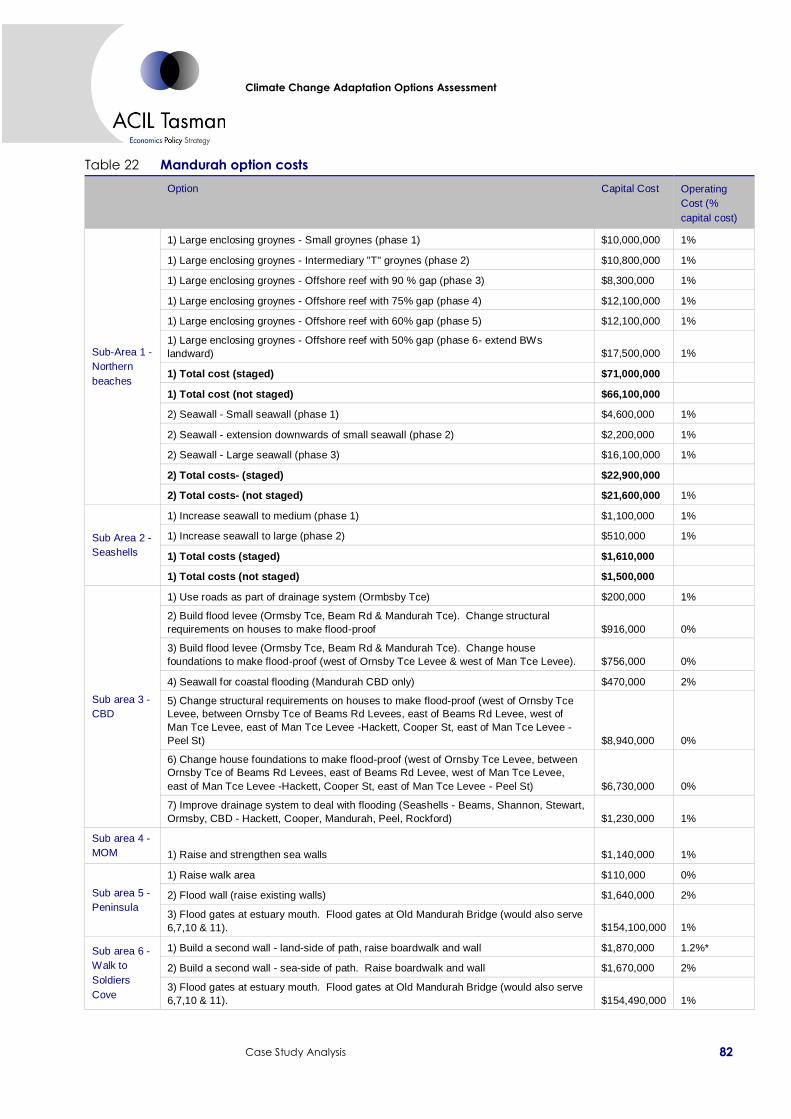
Climate Change Adaptation Options Assessment
Case Study Analysis 82
Table 22 Mandurah option costs
Option Capital Cost Operating
Cost (%
capital cost)
Sub-Area 1 -
Northern
beaches
1) Large enclosing groynes - Small groynes (phase 1) $10,000,000 1%
1) Large enclosing groynes - Intermediary "T" groynes (phase 2) $10,800,000 1%
1) Large enclosing groynes - Offshore reef with 90 % gap (phase 3) $8,300,000 1%
1) Large enclosing groynes - Offshore reef with 75% gap (phase 4) $12,100,000 1%
1) Large enclosing groynes - Offshore reef with 60% gap (phase 5) $12,100,000 1%
1) Large enclosing groynes - Offshore reef with 50% gap (phase 6- extend BWs
landward) $17,500,000 1%
1) Total cost (staged) $71,000,000
1) Total cost (not staged) $66,100,000
2) Seawall - Small seawall (phase 1) $4,600,000 1%
2) Seawall - extension downwards of small seawall (phase 2) $2,200,000 1%
2) Seawall - Large seawall (phase 3) $16,100,000 1%
2) Total costs- (staged) $22,900,000
2) Total costs- (not staged) $21,600,000 1%
Sub Area 2 -
Seashells
1) Increase seawall to medium (phase 1) $1,100,000 1%
1) Increase seawall to large (phase 2) $510,000 1%
1) Total costs (staged) $1,610,000
1) Total costs (not staged) $1,500,000
Sub area 3 -
CBD
1) Use roads as part of drainage system (Ormbsby Tce) $200,000 1%
2) Build flood levee (Ormsby Tce, Beam Rd & Mandurah Tce). Change structural
requirements on houses to make flood-proof $916,000 0%
3) Build flood levee (Ormsby Tce, Beam Rd & Mandurah Tce). Change house
foundations to make flood-proof (west of Ornsby Tce Levee & west of Man Tce Levee). $756,000 0%
4) Seawall for coastal flooding (Mandurah CBD only) $470,000 2%
5) Change structural requirements on houses to make flood-proof (west of Ornsby Tce
Levee, between Ornsby Tce of Beams Rd Levees, east of Beams Rd Levee, west of
Man Tce Levee, east of Man Tce Levee -Hackett, Cooper St, east of Man Tce Levee -
Peel St) $8,940,000 0%
6) Change house foundations to make flood-proof (west of Ornsby Tce Levee, between
Ornsby Tce of Beams Rd Levees, east of Beams Rd Levee, west of Man Tce Levee,
east of Man Tce Levee -Hackett, Cooper St, east of Man Tce Levee - Peel St) $6,730,000 0%
7) Improve drainage system to deal with flooding (Seashells - Beams, Shannon, Stewart,
Ormsby, CBD - Hackett, Cooper, Mandurah, Peel, Rockford) $1,230,000 1%
Sub area 4 -
MOM 1) Raise and strengthen sea walls $1,140,000 1%
Sub area 5 -
Peninsula
1) Raise walk area $110,000 0%
2) Flood wall (raise existing walls) $1,640,000 2%
3) Flood gates at estuary mouth. Flood gates at Old Mandurah Bridge (would also serve
6,7,10 & 11). $154,100,000 1%
Sub area 6 -
Walk to
Soldiers
Cove
1) Build a second wall - land-side of path, raise boardwalk and wall $1,870,000 1.2%*
2) Build a second wall - sea-side of path. Raise boardwalk and wall $1,670,000 2%
3) Flood gates at estuary mouth. Flood gates at Old Mandurah Bridge (would also serve
6,7,10 & 11). $154,490,000 1%

Climate Change Adaptation Options Assessment
Case Study Analysis 83
Sub area 7 -
SE canal
estate
1) Flood gates at estuary mouth. Flood gates at Old Mandurah Bridge (would also serve
6,7,10 & 11) $154,100,000 1%
2) Flood gates at estuary mouth and Dawesville Channel (would also serve 6,7,10 & 11) $132,600,000 1%
3) Sea wall prior to building houses. Fill low land $1,740,000 1.2%*
Sub area 8 -
Creery
Wetland
Foreshore
1) Strengthen embankment. Add wall.
$610,000 1.8%*
Sub area 9 -
SW canal
estates
1) Flood gates at estuary mouth and Dawesville Channel (would also serve 6,7,10 & 11) $132,600,000 1%
2) Flood gates at Old Mandurah Bridge and Dawesville Channel (would also serve
6,7,10 & 11) $193,500,000 1%
3) Sea wall prior to building houses / sea wall to prevent channel movement $1,100,000 1%
Sub area 10
- Port
Mandurah
1) Flood gates at Old Mandurah Bridge and Dawesville Channel (would also serve
6,7,10 & 11) $154,100,000 1%
2) Flood gates at estuary mouth and Dawesville Channel (would also serve 6,7,10 & 11) $132,600,000 1%
3) flood gates at entrance to residential canal area $43,000,000 1%
Sub area 11
- Western
Foreshore
1) Raise houses on foundations (progressive - at the end of each houses design life) $2,600,000 0%
2) Require zoning changes for new houses to flood-proof $6,600,000 0%
3) Crest wall $1,600,000 1%
4) flood gates at estuary mouth and Old Mandurah Bridge (would also serve 6,7,10 & 11) $154,100,000 1%
Sub area 12
- Halls Head
1) Large enclosing groynes - Small groynes (phase 1) $1,600,000 1%
1) Large enclosing groynes - Small groynes (phase 2) $1,300,000 1%
1) Large enclosing groynes - Intermediary "T" groynes (phase 3) $2,400,000 1%
1) Large enclosing groynes - Offshore reef with 50% gap (phase 4) $7,900,000 1%
1) Total cost (staged) $13,200,000
1) Total costs (not staged) $11,300,000 1%
2) Seawall - Small seawall (phase 1) $1,100,000 1%
2) Seawall - Extension downwards of small seawall (phase 2) $550,000 1%
2) Seawall – Large seawall (phase 3) $2,800,000 1%
2) Total costs- (staged) $4,450,000
2) Total costs- (not staged) $4,100,000 1%
Note: entries marked with a * are those where the individual elements have different operating costs and a weighted
average of the different elements is shown
Data source: Damara WA
In the coastal areas threatened with erosion, there are no “planning” options,
in the sense that we define them in Chapter 4. This is because erosion has
essentially two responses; either do something physical to prevent the erosion,
or do nothing and lose the land (a retreat option).
The engineering options for coastal areas all involve protection of some form
or another. There are three broad types of protection; seawalls, groynes and
offshore reefs (though not all are applicable in each case), and several levels of
protection in each case. The basic intuition is that one could begin relatively
small, but the relevant infrastructure would become inadequate at some point

Climate Change Adaptation Options Assessment
Case Study Analysis 84
in time, at which point it would be upgraded. Alternatively, one could start at a
large scale, which offers more permanent protection.
Sub Areas 1,2, 4 and 12 would all require some form of engineering protection
against erosion. The full range of options could be employed in Sub Area 1.
However, Sub Areas 2 and 4 already have sea walls (in Sub Area 4, the outer
wall of the marina) meaning the focus would be on strengthening rather than
new construction, and in Sub Area 12, the need to trap sediment for
redistribution means that offshore reefs are not appropriate.
Sub Area 2 is subject to flooding as well as erosion. In particular, there is a
long thin finger of low-lying land behind the (now built-over) dune system
which is at risk. This could be protected by a levee or, since it is some time
before the flood risk is realised, by planning requirements that require all new
buildings to be flood-proofed. If we assume (see AECOM, 2010) an average
building life of 40 years, then implementing these requirements would mean
that 2.5 per cent of buildings are raised every two years on an assumption of
evenly distributed ages of buildings.
Within the CBD in Sub Area 3, there is less scope for a planning solution
requiring flood proofing because of the heterogeneous uses of land within the
precinct, which makes it more difficult to implement such a planning response
compared to the predominantly residential Sub Area 2. Its longer sea-frontage
makes a levee more expensive, and has visual amenity issues in what is
primarily foreshore park. However, a seawall for coastal flooding as part of a
promenade may prove a suitable alternative. Note in Sub Area 3 that the low
cost of using roads as part of the drainage system is based on a marginal cost
assumption; that is, that the relevant engineering work needed to do this would
be undertaken at the time when the roads were due for an upgrade or
maintenance in any case.
Sub Area 5 presents particular problems because commercial development is
very close to the water’s edge. This means that anything larger than a relatively
small flood wall would be untenable, and this may be insufficient to protect the
developments in the event of a large flood. This means that the option as
presented is not “optimal” in the sense that it will not offer full protection for
this asset. In the longer term, it may be appropriate to change the
requirements for new commercial buildings in the area to require them to build
flood-protection into the building design, and to negotiate with existing
commercial developments to retro-fit the same (where possible) in a cost-
effective manner. A final option for this sub area, which would also influence
flood risk in Sub Areas 6,7,8,9,10 and 11 as well could be to put flood gates at
the estuary mouth and at the old and new Mandurah Bridges. A gate at the old
bridge would protect Sub Area 5 and part of Sub Area 11, while one at the new
bridge would protect all sub areas except 8 and 9 and part of 7; to protect these

Climate Change Adaptation Options Assessment
Case Study Analysis 85
using flood gates would require a flood gate at the Dawesville Cut or a
narrowing of the channel, both of which are very expensive options but one
with impacts throughout the estuary.
Sub Areas 6 and 8 are similar in that they have foreshore reserves with existing,
albeit low walls that could be strengthened. Sub Area 11 is also mostly
parkland. However, it also contains houses in its northern extremity.
Sub Areas 7, 9 and 10 present similar problems in that they are canal estates.
In Sub Area 9, we understand that there are existing plans to fill the areas
where flooding is a risk. However, it may also require a seawall to prevent
movement of the channel. Sub Area 10 has the advantage that, although it is a
canal estate, there are only two entrances to the estuary, and it may thus be
possible to install flood gates across the entrances and protect the
development. The same is true of the northern part of Sub Area 7, but not of
the southern part, which looks over wetlands. For all three canal estates, an
issue exists in that private land extends to the waterline, meaning that solutions
within each estate would need to be carried out by landowners, rather than
government.
Options and optimal timing results
Table 23 provides an overview of the options that are viable in Mandurah in an
economic sense. By viable, we mean that the options are chosen in at least
some of the scenarios by the real options algorithm, at some year during the
100-year timeframe under analysis. Table 23 shows the capital cost of each
option, its operating cost, the optimal year for implementing the option and
the net benefit (the reduction in value at risk it provides minus the cost of the
option) in produces. The final column shows the percentage of scenarios in
which the option is viable (as defined above). It is worth noting that the
optimal year and net benefit results for each option are based on the viable
realisations of that option. Thus, in some instances, where an option is only
viable in a small number of scenarios, these results can be skewed. This is
discussed further below.

Climate Change Adaptation Options Assessment
Case Study Analysis 86
Table 23 Mandurah viable options summary
Option Capital Cost OPEX
Optimal
Year Net benefit
% let expire
scenarios
Sub-Area 1 - Northern
beaches
1 $10,000,000 $100,000 12 $35,755,000 25.70%
2 $10,800,000 $108,000 30 $13,599,000 16.00%
3 $8,300,000 $83,000 38 $10,552,000 6.00%
4 $12,100,000 $121,000 57 $1,674,000 80.00%
5 $12,100,000 $121,000 57 $1,674,000 80.00%
7 $66,100,000 $708,000 8 $28,511,000 55.00%
8 $4,600,000 $46,000 23 $4,979,000 92.20%
9 $2,200,000 $22,000 12 $34,310,000 28.30%
10 $16,100,000 $161,000 26 $19,850,000 6.40%
11 $21,600,000 $229,000 11 $50,898,000 4.00%
Sub Area 2 -
Seashells
1 $1,100,000 $11,000 8 $11,855,000 38.00%
2 $510,000 $5,100 23 $10,863,000 0.00%
3 $1,500,000 $16,100 7 $27,132,000 2.30%
Sub area 3 - CBD
1 $200,000 $2,000 49.5 $1,127,000 0.00%
2 $916,000 $- 68 $437,000 0.00%
3 $756,000 $- 68 $459,000 0.00%
4 $470,000 $9,400 67 $496,000 0.00%
7 $1,230,000 $12,300 53 $893,000 0.00%
Sub area 4 - MOM 1 $1,140,000 $14,500 3.5 $61,247,000 5.80%
Sub area 5 -
Peninsula
1 $110,000 $-
2 $1,670,000 $28,400 67 $319,000 0.00%
Sub area 7 - SE canal
estate 3 $1,740,000 $28,000 65 $534,000 0.00%
Sub area 8 - Creery
Wetland Foreshore 1 $610,000 $10,900 57 $102,000 0.00%
Sub area 9 - SW
canal estates 3 $1,100,000 $11,000 41 $1,331,000 0.00%
Sub area 11 -
Western Foreshore
1 $2,600,000 $- 59 $439,000 0.00%
3 $1,600,000 $16,000 56.5 $617,000 0.00%
Sub area 12 - Halls
Head
1 $1,600,000 $16,000 8 $1,291,000 85.70%
2 $1,300,000 $13,000 20.5 $881,000 79.70%
3 $2,400,000 $24,000 18.5 $1,285,000 62.30%
4 $7,900,000 $79,000 14 $1,226,000 96.10%
5 $11,300,000 $122,000 2.5 $1,353,000 95.60%
6 $1,100,000 $11,000 10.5 $753,000 93.50%
7 $550,000 $5,500 12 $3,331,000 34.20%
8 $2,800,000 $28,000 25.5 $1,713,000 20.40%
9 $4,100,000 $44,500 5 $5,615,000 12.50%
Climate Change Adaptation Options Assessment
Case Study Analysis 87
Mandurah is the most complex of the case studies, and we divide the
discussion in three; an overview of the coastal sub-areas (1,2,4 and 12), an
overview of the inland or estuarine sub areas and a discussion of the impacts of
sand replenishment on the coast as an option.
Coastal areas
Within the coastal areas, Sub Areas 1 and 12 have the option of using groynes
or seawalls, while Sub Areas 2 and 4, which already have some existing seawall
structures, only have the option of extending their seawalls.
Groynes, in Sub Areas 1 and 12, are roughly three times the cost of seawalls.
In the case of Sub Area 12, the value of the asset being saved means that the
more expensive groynes are not the preferred option (note the large “let
expire” percentages), and the relevant choice is between staging the seawall, or
building it all at once. Note that staging is more valuable; roughly $59 million
in sum across the three stages compared with $51 million for constructing the
walls all at once.
In Sub Area 1, the more valuable asset means that groynes are feasible.
However, only the first three stages of the groynes are viable, with the fourth
stage expiring in 80 per cent of scenarios. This is shown clearly in Figure 6,
which charts the distribution of optimal times (across scenarios) for the first
four stages.59 Note how the distribution becomes more spread out, as well as
smaller, as the investment cost increases.
59 For reasons of space restrictions, the axes are unlabelled in Figure 6. However, each picture
is a histogram showing the number of scenarios (the vertical axis) where the given option is optimal in the corresponding year, shown on the horizontal axis.

Climate Change Adaptation Options Assessment
Case Study Analysis 88
The basic issue is the extent of erosion risk. The first three stages of the
groynes provide protection up to an erosion level of 50 per cent, the number
of scenarios (and extent of exceedance) which exceed this amount is
insufficient to warrant the additional expenditure. The same effect is not seen
in seawalls, as the first two stages only provide protection up to 17 per cent
erosion, meaning the third stage is viable.
In comparing the first three stages of the groyne options with the seawall
option (also in three stages), the groyne option provides a slightly higher net
benefit, meaning society would be slightly better off by adopting this option.
However, the cost of the option is much higher, and for this reason, it is likely
that seawalls would be a preferable option to groynes, if cost and risk are the
only considerations.
Sub Area 12 and Sub Area 2 both highlight a similar issue in their first stage;
their first stages are only viable in a small number of scenarios. This is because
the seawalls in their first stages only provide protection up to seven per cent
erosion, and with the rise in sea levels in the scenarios, this proves to be too
little, resulting in the first stage soon needing to be replaced by a second stage.
This means that the value at risk savings are generally too small to make the
Figure 6 Mandurah northern beaches sub area groynes options – histograms of optimal timing
0
50
100
150
200
250
300
1 5 9
13
17
21
25
29
33
37
41
45
49
53
57
61
65
69
73
77
81
85
89
93
Let
exp
ire
Option One
0
20
40
60
80
100
120
140
160
1 5 9
13
17
21
25
29
33
37
41
45
49
53
57
61
65
69
73
77
81
85
89
93
Let
exp
ire
Option Two
0
10
20
30
40
50
60
70
80
1 5 9
13
17
21
25
29
33
37
41
45
49
53
57
61
65
69
73
77
81
85
89
93
Let
exp
ire
Option Three
0
100
200
300
400
500
600
700
800
900
1 5 9
13
17
21
25
29
33
37
41
45
49
53
57
61
65
69
73
77
81
85
89
93
Let
exp
ire
Option Four
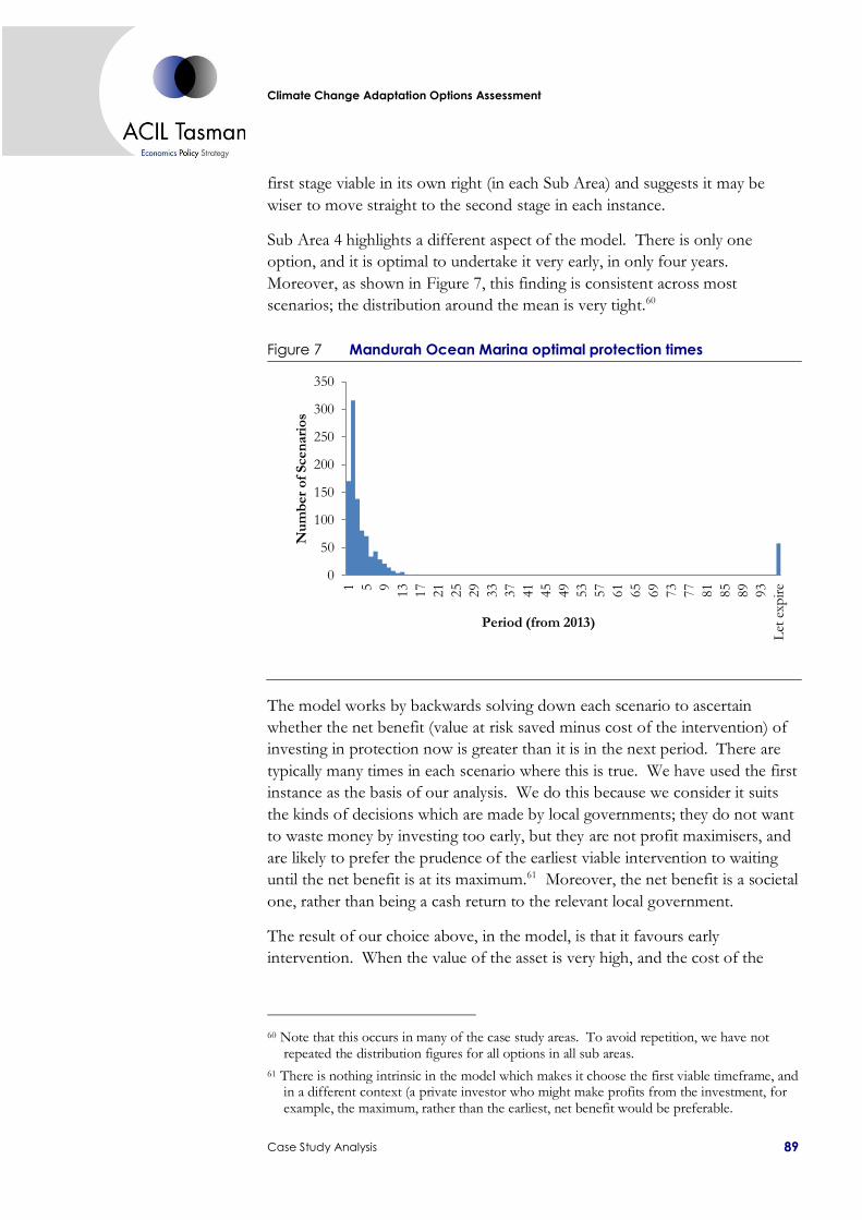
Climate Change Adaptation Options Assessment
Case Study Analysis 89
first stage viable in its own right (in each Sub Area) and suggests it may be
wiser to move straight to the second stage in each instance.
Sub Area 4 highlights a different aspect of the model. There is only one
option, and it is optimal to undertake it very early, in only four years.
Moreover, as shown in Figure 7, this finding is consistent across most
scenarios; the distribution around the mean is very tight.60
Figure 7 Mandurah Ocean Marina optimal protection times
The model works by backwards solving down each scenario to ascertain
whether the net benefit (value at risk saved minus cost of the intervention) of
investing in protection now is greater than it is in the next period. There are
typically many times in each scenario where this is true. We have used the first
instance as the basis of our analysis. We do this because we consider it suits
the kinds of decisions which are made by local governments; they do not want
to waste money by investing too early, but they are not profit maximisers, and
are likely to prefer the prudence of the earliest viable intervention to waiting
until the net benefit is at its maximum.61 Moreover, the net benefit is a societal
one, rather than being a cash return to the relevant local government.
The result of our choice above, in the model, is that it favours early
intervention. When the value of the asset is very high, and the cost of the
60 Note that this occurs in many of the case study areas. To avoid repetition, we have not
repeated the distribution figures for all options in all sub areas.
61 There is nothing intrinsic in the model which makes it choose the first viable timeframe, and in a different context (a private investor who might make profits from the investment, for example, the maximum, rather than the earliest, net benefit would be preferable.
0
50
100
150
200
250
300
350
1 5 9
13
17
21
25
29
33
37
41
45
49
53
57
61
65
69
73
77
81
85
89
93
Let
exp
ire
Nu
mb
er
of
Scen
ari
os
Period (from 2013)

Climate Change Adaptation Options Assessment
Case Study Analysis 90
intervention is very low (as is the case in Sub Area 4), the net result is an
optimal investment time which appears very early in the context of the
engineering information about coastal erosion presented in the Phase One
report. One way of considering strategy based upon this is that it represents
the earliest viable time to intervene, not the last possible moment in which one
ought to do so.
In each of the coastal areas, the intervention times are several years hence,
during which time erosive pressures are likely to occur. However, except in
the case of Sub Area 12, existing structures are in place. In Sub Area 12,
around five per cent of the sub area would be lost to erosion by the time it
becomes optimal to construct the sea wall. This equates to around 15 metres
of beach (no houses would be affected), which could either be sacrificed or
maintained through sand replenishment (see discussion on sand replenishment
as an option below).
Estuarine areas
Moving now to the inland (or rather estuarine) regions, we begin with Sub
Area 3 in the CBD. Here the model suggests starting with Option One in 50
years, and moving to either of Options Two, Three or Four in around 65 years.
Each of these subsequent options has the same profit (slightly less than
$500,000) and thus, since they are direct substitutes for each other, it appears
wise to use the lowest-cost option, Option Four.
Some care needs to be used when interpreting the model results for Sub Area
3. The first option lasts 50 years, and needs to be implemented in 50 years,
while the latter three last for 30 years, and need to be implemented in slightly
under 70 years. This suggests that the chosen end point of the engineering
analysis (the NPV calculations go out 500 years, but there is no change in
erosion or flooding after year 100) may be influencing results. Changing the
approach to allow erosion and flooding after 2110 may result in a later
intervention.
For Sub Areas 4 and 5, there is only a single optimal choice. In Sub Area 4,
there is only one choice, and in Sub Area 5, although the first two options are
viable, the first lasts for 100 years and costs only $110,000, while the second
lasts for only 30 years and lasts for only 30 years. In the case of Sub Area 5,
however, it should be noted that none of the solutions “solve” the problem
completely in the sense that the location of the commercial properties in the
sub area preclude the construction of defensive measures that will be fully
effective. In the longer term, a solution will have to be reached with property
owners and lease-holders in this sub area to re-design their properties to
account for flood protection measures.

Climate Change Adaptation Options Assessment
Case Study Analysis 91
Sub Areas 6 and 10 both have no action as the modelling result; none of the
options that are feasible from an engineering sense are feasible from an
economic sense. Sub Area 10 is perhaps of the greatest interest in this respect,
as it is a canal estate, dominated by private property, and thus it would seem a
simple matter if the residents of that region value their properties more highly
than we have done in our assessment to collectively implement the proposed
measures. However, we note that the extent of flooding predicted by the
models in this area is not sufficient to result in the potential loss of houses.
Rather, it is sufficient to result in the loss of gardens, jetties and structures at
the waterline. The residents in question may decide to wear this loss, rather
than paying to protect the whole area via the flood-gates or other measures
suggested above.
Sub Areas 7and 9 are similar in that each has one very low cost option and two
very high cost options; the gating of either the Dawesville Cut, the Old
Mandurah Bridge or the estuary mouth. The result is a clear preference for the
much cheaper option (see Box 5 for more detail). In the case of Sub Area 7,
the model suggest implementation in 65 years and for Sub Area 9 it suggests
action in 41 years. However, in both cases, the relevant measures need to be
taken before the houses are built, after which time they become impossible. It
seems unlikely, given growth in the area, that developers will wait this long
before building in these areas, regardless of our model results, and this may
mean that the City of Mandurah needs to consider requiring the relevant action
to be taken by the developer prior to any more development occurring.
Sub Area 8 has a single option, which the model suggests ought to be
implemented in 57 years.
Finally, Sub Area 11 has three low cost options and one very costly one (flood
gates). Of the three less costly ones, a crest wall would be insufficient to meet
the rising risks, and would fail too quickly to deliver value at risk savings. The
two options involving raising the houses as they are renewed would both be
optimal at around the same time (56 and 58 years from now respectively), and
both would have roughly the same profit ($400 and $600,000 respectively).
This suggests that the less expensive option, Option 1, would be the better
choice. As a final point, it is worth noting that the low costs are achieved by
fixing each house as it reaches the end of its operational life and is renewed. In
the model, the options are shown as being optimal in 56 and 58 years.
However, in reality, since an average house lasts around 40 years, the City
would need to change its building requirements is around 15 years to ensure
that the option is complete by the time it is needed.
Climate Change Adaptation Options Assessment
Case Study Analysis 92
Box 5 Flood gates
There are several “large-scale” options involving flood gates at the estuary mouth, the
Old Mandurah Bridge and the Dawesville Cut (which could also be narrowed). In the
modelling, we assessed each of these against each of the individual sub-areas, and it
was never optimal to implement any of them to save a single sub-area. However, each
of these options would save several sub-areas in conjunction. We did not model these
large-scale options against several sub-areas in conjunction. The reason for doing this is
that the flood gates and channel narrowing are more than twice as expensive as all of
the other options which could be used to protect the relevant regions put together (and
two-thirds of that cost is flood gates in Sub Area 10, which are not optimal either). Since
each sub area has an optimal solution which is much less expensive than the large,
region-wide structures, there is little benefit in employing them at this stage. They would
rather become viable for a two-metre, rather than a one-metre sea level rise. The
caveat, however, is that our conclusion is based upon the value of the assets in the case
study area alone, and such structures would act to protect the whole estuary. A wider
scale of analysis may conclude that they are viable.
Sand replenishment as an option
For each of the coastal areas subject to erosion where seawalls are used, the
land will be protected, but not the beach. We therefore examine the option of
sand replenishment. The cost of sand replenishment is roughly $2.6 million
for every one per cent of erosion; the more the erosive pressure, the more sand
would need to be replenished in order to keep the beach (and the land behind
it) in place.
We consider the case of Sub Area 1, as it is the area which is the most valuable.
However, the findings are generalizable to other assets. The cost of sand
replenishment is $2.637 million per percentage point of erosion (more
correctly, erosive pressure, through sea-level rise) in Sub Area 1. As sea levels
rise, more and more sand will need to be put onto the beach in order to
protect it. In reality, some sand will be eroded from year to year, in between
replenishment episodes, increasing the amount that would need to be put onto
a beach. However, if we adopt a more conservative approach, and assume that
new sand is needed only for incremental erosive pressure, the annual cost of
replenishment is as shown in Figure 8 for Sub Area 1.

Climate Change Adaptation Options Assessment
Case Study Analysis 93
Figure 8 Annual cost of sand replenishment – Sub Area 1
On average, the figure is between $1.5 and $2 million per annum, which
equates to around $51 million in net present value terms over the hundred-year
time horizon. This makes it much more expensive than any of the other
options, even before we consider whether sufficient sand would in fact be
available, and thus it would not be an optimal solution compared to the other
measures suggested above.
Another consideration with sand replenishment is that the seawall (or groynes)
could be used to protect the land, and sand replenishment could be used to
provide a beach for the community; absent of sand replenishment, beaches
would vanish, particularly if a seawall was used. In this instance, the value of
the beach would need to warrant the replenishment expenditure.
In Sub Area 1, the beach alone is worth $6 million, or $180,000 per annum,
and thus the cost of replenishment would be around ten times the economic
value of the beach by the time the seawall was put in place. This means that
the community would need to consider how its valuation of the beach differs
for our own, and whether it is willing to fund its continuation under a scenario
involving these kinds of costs.
Formulation of options pathways
In most of the sub areas, there is only one option that is viable or, if there are
two, they are substitutes rather than complements. The exceptions are Sub
Areas 1 and 12, where the different options are staged.
For these options, we look at the first stage, considering when it is optimal.
Then, in looking at the second stage, we assume stage one is in place, offering
$-
$500,000
$1,000,000
$1,500,000
$2,000,000
$2,500,000
$3,000,000
$3,500,000
20
13
20
18
20
23
20
28
20
33
20
38
20
43
20
48
20
53
20
58
20
63
20
68
20
73
20
78
20
83
20
88
20
93
20
98
21
03
21
08

Climate Change Adaptation Options Assessment
Case Study Analysis 94
a level of protection for a period of time, until the erosive pressures are too
great (or design life is exceeded, which does not happen in practice), and then
the optimal time to put the second stage in place is then the first time after the
“failure point” that the net benefit is positive.
This optimal second stage can result in some erosion in the interim, depending
upon the optimal timing of the second stage. However, in this case, the model
results indicate a gap of only a year in each case, which effectively means no
erosion.
Note that the approach above is subtly different from the description in
Section 5.1, in that we have effectively used an American option approach
twice, rather than the European option approach noted above. We did this
because the relevant pressure for the second stage was not the design life of
the structure, but the degree of erosive pressure it can withstand, and this is
different in every scenario.
5.3 Case Study Two: Siesta Park-Marybrook
This case study runs from the Lennox Drain to the Buayanup Drain (from
Forth St to Mitchell St) along Caves Road, and extends inland almost two
kilometres, covering farmland that would be affected by flooding. The land
uses are residential along the coast, and farming land inland from the coast.
The residential land uses are the least dense amongst the case study areas.
However, some of the residential land, particularly in Siesta Park, is very
valuable; to the point that some land-owners have already begun to install their
own seawalls to protect their property. The sub-areas are described in Table
24, and shown in Figure 9.

95
Ca
se S
tud
y A
na
lysis
Clim
ate
Ch
an
ge
Ad
ap
tatio
n O
ptio
ns A
ssessm
en
t
Table 24 Summary of asset values in Siesta-Park-Marybrook
Asset classing 1 2 3 4 5
West of Siesta Park Siesta Park Locke Estate W. Buayanup Lennox Drain
area (m2) unit value of
asset value of sub-area area (m2)
unit value of
asset value of sub-area area (m2)
unit value of
asset value of sub-area area (m2)
unit value of
asset value of sub-area area (m2) unit value of asset value of sub-area
Roads (m) one lane 0 275$ -$ 0 275$ -$ 0 275$ -$ 0 275$ -$ 0 275$ -$
two or more lanes 1054.2 360$ 379,511$ 1585.6 360$ 570,809$ 1467.5 360$ 528,309$ 885.3 360$ 318,694$ 43.0 360$ 15,464$
Water (m) mains 1053.9 450$ 474,258$ 1579.6 450$ 710,829$ 1432.3 450$ 644,536$ 884.4 450$ 397,964$ 30.1 450$ 13,546$
Electricity low voltage (m) underground 157.3 150$ 23,602$ 142.6 150$ 21,397$ 86.1 150$ 12,919$ 0.0 150$ -$ 0.0 150$ -$
overhead 930.6 45$ 41,876$ 597.0 45$ 26,865$ 607.3 45$ 27,326$ 903.6 45$ 40,662$ 31.5 45$ 1,419$
Electricity high voltage (m) underground 75.7 300$ 22,715$ 0.0 300$ -$ 0.0 300$ -$ 0.0 300$ -$ 8.0 300$ 2,400$
overhead 1652.6 55$ 90,892$ 967.1 55$ 53,189$ 2332.0 55$ 128,261$ 904.4 55$ 49,742$ 246.8 55$ 13,576$
Commercial land (ha) 0 16,672,800$ -$ 6.5 16,672,800$ 108,557,142$ 0.0 16,672,800$ -$ 0.0 16,672,800$ -$ 0.0 16,672,800$ -$
Residential land (ha) 8.0 13,750,000$ 109,659,205$ 11.9 13,750,000$ 163,443,906$ 2.2 5,734,375$ 12,395,499$ 0.0 5,734,375$ -$ 0.0 -$ -$
Development land (ha) 0 -$ -$ 0.0 -$ -$ 0.0 -$ -$ 0.0 -$ -$ 0.0 -$ -$
Agricultural land (ha) 38.3 25,100$ 962,054$ 25.4 25,100$ 638,218$ 19.1 25,100$ 478,765$ 0.0 25,100$ -$ 7.6 25,100$ 190,621$
Community infrastructure (ha) 0.4 4,395,300$ 1,740,176$ 0.0 4,395,300$ -$ 13.1 5,734,375$ 74,873,817$ 21.8 5,734,375$ 125,202,335$ 8.7 5,734,375$ 50,155,474$
Parks, recreational and conservation areas (ha) 4.5 1,375,000$ 6,246,767$ 6.5 1,375,000$ 8,893,491$ 28.7 573,438$ 16,481,455$ 25.8 573,438$ 14,793,549$ 0.1 573,438$ 55,455$
Beaches (m) 1019 900$ 917,100$ 929 900$ 836,100$ 1131.0 900$ 1,017,900$ 843 900$ 758,700$ 0 900$ -$
Total 51 120,558,157$ 50 283,751,946$ 63 106,588,787$ 48 141,561,646$ 16 50,447,956$
Asset classing 6 7 8 9 Total
W. Wetland Locke Drain E. Wetland Buayanup Drain
area (m2)
unit value of
asset value of sub-area area (m2)
unit value of
asset value of sub-area area (m2)
unit value of
asset value of sub-area area (m2)
unit value of
asset value of sub-area area (m2)
value of case study
area
Roads (m) one lane 0 275$ -$ 0 275$ -$ 0 275$ -$ 4.0 275$ 1,100$ 4 1,100$
two or more lanes 0 360$ -$ 16.5 360$ 5,923$ 0 360$ -$ 35.9 360$ 12,907$ 5088 1,831,617$
Water (m) mains 0 450$ -$ 17.7 450$ 7,956$ 0 450$ -$ 41.0 450$ 18,462$ 5039 2,267,551$
Electricity low voltage (m) underground 0 150$ -$ 0.0 150$ -$ 0 150$ -$ 0.0 150$ -$ 386 57,918$
overhead 0 45$ -$ 0.0 45$ -$ 0 45$ -$ 27.1 45$ 1,220$ 3097 139,369$
Electricity high voltage (m) underground 0 300$ -$ 4.0 300$ 1,200$ 0 300$ -$ 12.0 300$ 3,609$ 100 29,925$
overhead 425.8 55$ 23,422$ 16.4 55$ 900$ 0 55$ -$ 104.1 55$ 5,728$ 6649 365,710$
Commercial land (ha) 0.0 16,672,800$ -$ 0.0 16,672,800$ -$ 0 16,672,800$ -$ 0.0 16,672,800$ -$ 7 108,557,142$
Residential land (ha) 0.0 -$ -$ 0.0 -$ -$ 0 -$ -$ 0.0 -$ -$ 22 285,498,610$
Development land (ha) 0.0 -$ -$ 0.0 -$ -$ 19.0 5,734,375$ 109,152,059$ 0.1 5,734,375$ 829,293$ 19 109,981,352$
Agricultural land (ha) 253.5 25,100$ 6,362,561$ 4.1 25,100$ 103,567$ 72.9 25,100$ 1,829,538$ 1.6 25,100$ 40,070$ 423 10,605,393$
Community infrastructure (ha) 1.1 4,395,300$ 4,978,139$ 0.5 4,395,300$ 2,113,705$ 0.0 4,395,300$ -$ 1.9 4,395,300$ 8,150,549$ 48 267,214,196$
Parks, recreational and conservation areas (ha) 20.4 573,438$ 11,717,069$ 1.0 573,438$ 586,036$ 142.6 573,438$ 81,775,423$ 0.2 573,438$ 139,802$ 230 140,689,048$
Beaches (m) 0 900$ -$ 47 900$ 42,300$ 0 900$ -$ 47 900$ 42,300$ 4016 3,614,400$
Total 275 23,081,191$ 6 2,861,586$ 235 192,757,020$ 4 9,245,041$ 748 930,853,329$

Climate Change Adaptation Options Assessment
Case Study Analysis 96
Figure 9 Siesta Park/ Marybrook case study sub-areas
The coastal areas are divided into four. The first two of these when moving
from east to west contain the “Holy Mile”; land leased to various church
bodies an community organisations, and used primarily for camping and other
church group activities. This land is less valuable than the remaining two
coastal areas, but this is largely a by-product of its zoning; if the leases were
changed, the land would become more valuable immediately, as it was sought
for re-development in the same way as other areas along the coast.62
The remaining two areas contain more valuable private real estate, particularly
in Sub Area 1, where several householders have constructed their own seawalls
(which are not always effective). Sub Area 2 also contains a groyne, which has
retained sediment within this sub area, to the detriment of Sub Area 3
immediately to its east.
Inland, three of the sub areas (5, 7 and 9) are drainage culverts, which drain
run-off from surrounding farmland to the sea. Sub Areas 5 and 9 (Lennox and
Buayanup Drain respectively) already have levees, while Sub Area 7 (Locke
Drain) does not. Sub Areas 6 and 8 are predominantly low-lying nature
reserves or farmland; though there is a school and newly-created residential
development just outside the south eastern corner of Sub Area 8, whose
expansion would clearly need to be considered in the light of flood risk
findings in this report.
62 This land is termed “community use in the planning schemes, and we value it according to
residential, rather than commercial land in this instance, to take account of its next best alternate use.

Climate Change Adaptation Options Assessment
Case Study Analysis 97
Climate change impacts in the Siesta Park-Marybrook case study
The danger along the coast is erosion, with the model predicting around 300
metres of land vanishing by 2100. This would result in the loss of all of the
residential areas and Caves Road. However, an important caveat to the model
results is that the results for Busselton may overstate the impacts (see Phase
One Report for details
In the Mandurah case study area, seawater flooding had a temporary effect, for
the most part, because the areas affected are predominantly residential. Thus,
houses are flooded, but can be repaired and rebuilt soon after the flood has
finished. Sub Areas 6 and 8 are different because they are agricultural land. If
they are flooded by seawater, once the flood waters evaporate, the land is left
contaminated by salt, and may be rendered unusable for a number of years.
This necessitates a different treatment of the value at risk compared with
Mandurah. We explore two different possibilities, either allowing some of the
land to become salt-affected and protecting the rest with a levy or pumping
freshwater into the low-lying areas to create freshwater lakes and prevent salt-
water intrusion.
Description of options
The options for the different areas are shown in Table 25 below.
For the coastal areas, the options are essentially the same as those for coastal
areas in Mandurah, with the exception that we have considered individual sea
walls for the affected properties, as many of the properties have sea-frontage,
and some are already suing these seawalls on an ad-hoc basis. The difference is
that there is not a need to go to the same extent in terms of scale, because the
risks are slightly lower, and the number of properties affected are smaller. The
only differences between the four areas are that Sub Area 2 already has a
groyne, which could be extended, and that differing land values may make
retreating a more palatable option in some areas than in others. Also,
compared with other case studies, in this case, the affected land is almost
entirely privately held (along the coast), which makes it both easier and more
appropriate (in an efficient resource allocation sense) for private land-holders
to pay for any protection through dedicated levies if the City of Busselton so
chooses. A final issue in relation to the coast is Caves Road, which is a major
access road which would most likely need to be protected to maintain the
integrity of the transport system.

Climate Change Adaptation Options Assessment
Case Study Analysis 98
Table 25 Siesta Park Marybrook options summary
Sub Area Option
Capital Cost Operating
Cost (%
capital cost)
Sub area 1 - West of
Siesta Park
1) individual seawalls for each property $6,700,000 1.0%
2) single seawall across sub-region $4,800,000 1.0%
3) single large groyne $4,000,000 1.0%
4) multiple smaller groynes $2,000,000 1.0%
Sub area 2 - Siesta Park
1) individual seawalls for each property $5,500,000 1.0%
2) single seawall across sub-region $4,100,000 1.0%
3) extend existing groyne into single
large groyne $3,600,000 1.0%
4) multiple smaller groynes $1,900,000 1.0%
Sub area 3 - Locke Estate
1) individual seawalls for each property $6,100,000 1.0%
2) single seawall across sub-region $5,400,000 1.0%
3) single large groyne $4,300,000 1.0%
4) multiple smaller groynes $2,500,000 1.0%
Sub area 4 - W. Buayanup
1) individual seawalls for each property $4,900,000 1.0%
2) single seawall across sub-region $3,800,000 1.0%
3) single large groyne $3,400,000 1.0%
4) multiple smaller groynes $1,800,000 1.0%
Sub area 5 - Lennox Drain 1) put up gates to prevent storm surges
and raise levees $5,300,000 1.0%
Sub area 6 - W. Wetland
1) pump fresh water in to create lakes $14,600,000 1.0%
2) partition land to seal off lowest lying
areas an allow them to become salty $1,400,000 1.0%
Sub area 7 - Locke Drain 1) put up gates to prevent storm surges $2,000,000 1.0%
Sub area 8 - E. Wetland
1) pump fresh water in to create lakes $13,700,000 1.0%
2) partition land to seal off lowest lying
areas and allow them to become salty $1,400,000 1.0%
Sub area 9 - Buayanup
Drain 1) put up gates to prevent storm surges
and raise levees $3,000,000 1.0%
Data source: Damara WA
Inland, the flooding problem presents a different set of options. In the first
instance, Sub Areas 5, 7 and 9 would need gates at their mouths to prevent
storm surges sending salt water inland. Sub Areas 5 and 9 may also need to
have their levees improved to maintain their integrity.
For Sub Areas 6 and 8, there are two options. One is to compartmentalise
them, sealing off part of each (the lowest part) and allowing salt water to
intrude into that part as sea levels rise,63 but protecting the other part (which is
higher ground, and where the farmland is) from salt water intrusion. A second
63 Pushing salt water inland underground.

Climate Change Adaptation Options Assessment
Case Study Analysis 99
is to pump fresh water from the drains into the low-lying parts to prevent salt-
water intrusion from underground and to turn the wetlands into lakes. Each
would result in some land being sacrificed in order to save another portion of
land.
Options and optimal timing results
The model results are shown in Table 26.
Table 26 Siesta Park-Marybrook viable options summary
Sub area Option Capital cost OPEX
Optimal
Year Net benefit
% let expire
scenarios
Sub area 1 - West
of Siesta Park
3 $4,000,000 $40,000 4 $5,639,000 13.00%
4 $2,000,000 $20,000 4 $7,844,000 7.80%
Sub area 2 -
Siesta Park
3 $3,600,000 $36,000 15.5 $5,940,000 10.50%
4 $1,900,000 $19,000 15.5 $7,122,000 3.90%
Sub area 3 -
Locke Estate 4 $2,500,000 $25,000 37 $652,000 56.40%
Sub area 4 - W.
Buayanup
3 $3,400,000 $34,000 4 $5,842,000 13.80%
4 $1,800,000 $18,000 4 $7,578,000 9.70%
Sub area 5 -
Lennox Drain 1 $5,300,000 $53,000 14 $2,158,000 0.00%
Sub area 8 - E.
Wetland
1 $13,700,000 $137,000 1 $51,967,000 0.00%
2 $1,400,000 $14,000 1 $67,188,000 0.00%
Like Mandurah, there is a division between the coastal areas (Sub areas 1,2,3
and 4) subject to erosion, and the inland areas subject to flooding and salt-
water incursion.
For the coastal areas, Sub Area 1, 2 and 4 each have two options that are
viable, and Sub Area 3 has one. The lifespan of these options is the same in
each case, and within each sub area, each optimally begins at the same time.
Since the choice is between one or the other, there is no scope for staging or
combining the options.
In this situation, the most obvious was in which to make the choice is by
which provides the greatest net benefit. In each case the difference between
the better case and the less favourable case is around $2 million. In each of the
sub areas, it is the fourth option that is most valuable. It is also the least costly
option in each instance, making it the obvious choice.
In each of the coastal areas, it is important to consider how much erosion
might occur in the interim before the optimal response is made. This is
particularly the case for Sub Areas 2 and 3, where the optimal time to invest is
15 and 37 years respectively. Fortunately, in both of these areas, there is
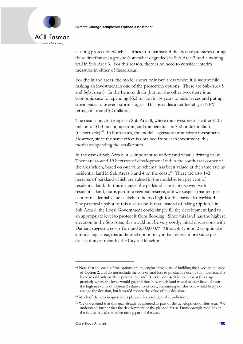
Climate Change Adaptation Options Assessment
Case Study Analysis 100
existing protection which is sufficient to withstand the erosive pressures during
these timeframes; a groyne (somewhat degraded) in Sub Area 2, and a training
wall in Sub Area 3. For this reason, there is no need to consider interim
measures in either of these areas.
For the inland areas, the model shows only two areas where it is worthwhile
making an investment in one of the protection options. These are Sub-Area 5
and Sub Area 8. In the Lennox drain (but not the other two, there is an
economic case for spending $5.3 million in 14 years to raise levees and put up
storm gates to prevent storm surges. This provides a net benefit, in NPV
terms, of around $2 million.
The case is much stronger in Sub Area 8, where the investment is either $13.7
million or $1.4 million up front, and the benefits are $52 or $67 million
(respectively).64 In both cases, the model suggests an immediate investment.
However, since the same effect is obtained from each investment, this
motivates spending the smaller sum.
In the case of Sub Area 8, it is important to understand what is driving value.
There are around 19 hectares of development land in the south-east corner of
the area which, based on our value schema, has been valued at the same rate as
residential land in Sub Areas 3 and 4 on the coast.65 There are also 142
hectares of parkland which are valued in the model at ten per cent of
residential land. In this instance, the parkland is not interwoven with
residential land, but is part of a regional reserve, and we suspect that ten per
cent of residential value is likely to be too high for this particular parkland.
The practical upshot of this discussion is that, instead of taking Option 2 in
Sub Area 8, the Local Government could simply fill the development land to
an appropriate level to protect it from flooding. Since this land has the highest
elevation in the Sub Area, this would not be very costly; initial discussions with
Damara suggest a cost of around $500,000.66 Although Option 2 is optimal in
a modelling sense, this additional option may in fact derive more value per
dollar of investment by the City of Busselton.
64 Note that the costs of the options are the engineering costs of building the levees in the case
of Option 2, and do not include the cost of land lost to productive use by salt incursion; the levee would only partially protect the land. This is because it is not clear at this stage precisely where the levee would go, and thus how much land would be sacrificed. Given the high net value of Option 2 relative to its cost, accounting for this cost would likely not change the decision, but it would reduce the value of this decision.
65 Much of the area in question is planned for a residential sub-division.
66 We understand that this may already be planned as part of the development of this area. We understand further that the development of the planned Vasse-Dunsborough road link in the future may also involve raising part of the area.

Climate Change Adaptation Options Assessment
Case Study Analysis 101
It is worth noting that, even if Option 2 is chosen for Sub Area 8, the net
effect in the case study area as a whole will be to not protect the lower-lying
agricultural land in the area, which could be subject to salt-incursion. From an
economic perspective, the land is not sufficiently value in its use as agricultural
land to warrant the rather costly protection measures that would be required.
This is an issue which would need to be considered by the City of Busselton in
more detail, as to whether there are sufficient non-economic reasons to
warrant spending the funds necessary to save the relevant farmland. This
investigation ought to also consider in more detail how much farmland would
need to be sacrificed, which has not been possible in this study.
Formulation of options pathways
Each sub area has a single option which is viable or, where there are two viable
options, they are substitutes rather than complements. For this reason, it is not
necessary to consider pathways comprising combinations of options.
5.4 Case Study Three: Peppermint Grove Beach
The third case study is the settlement of Peppermint Grove Beach. The case
study area runs from the area of agricultural land (Stirling Estate) just to the
north of the settlement, down to Higgins Cut at the southern end of the
settlement, and inland to approximately Ludlow Road North, taking in the
low-lying land immediately behind the dunes upon which the settlement is
built. The case study area has been divided into seven sub sections which are
summarised in Table 27 and shown in Figure 10.

102
Ca
se S
tud
y A
na
lysis
Clim
ate
Ch
an
ge
Ad
ap
tatio
n O
ptio
ns A
ssessm
en
t
Table 27 Summary of asset values in Peppermint Grove Beach
Asset classing 1 2 3 4
Northern wetlands Levee system Southern wetlands Higgins Cut
area
(m2)
unit value of
asset
value of sub-
area
area
(m2)
unit value of
asset
value of sub-
area
area
(m2)
unit value of
asset
value of sub-
area
area
(m2)
unit value of
asset
value of sub-
area
Roads (m) one lane 0 275$ -$ 0 275$ -$ 4267.2 275$ 1,173,480$ 0 275$ -$
two or more lanes 522.6 360$ 188,136$ 271.4 360$ 97,704$ 1415.9 360$ 509,724$ 160.3 360$ 57,708$
Water (m) retic 0 428$ -$ 0 428$ -$ 145.6 428$ 62,244$ 0 428$ -$
Electricity low voltage (m) underground 0 150$ -$ 0 150$ -$ 115.6 150$ 17,340$ 0 150$ -$
overhead 0 45$ -$ 0 45$ -$ 72.1 45$ 3,245$ 0 45$ -$
Electricity high voltage (m) underground 0 300$ -$ 0 300$ -$ 1004.1 300$ 301,230$ 0 300$ -$
overhead 552.6 55$ 30,393$ 163.2 55$ 8,976$ 2484.5 55$ 136,648$ 162.9 55$ 8,960$
Residential land (ha) 0 -$ -$ 0 -$ -$ 2.6 6,250,000$ 16,250,000$ 3.6 6,250,000$ 22,500,000$
Rural land (ha) 95.7 33,500$ 3,205,950$ 11.7 33,500$ 391,950$ 395 33,500$ 13,232,500$ 17.8 33,500$ 596,300$
Agricultural land (ha) 4.8 33,500$ 159,982$ 3.3 33,500$ 110,640$ 0 33,500$ -$ 0 33,500$ -$
Community infrastructure (ha) 0 -$ -$ 0 6,250,000$ -$ 11.7 6,250,000$ 6,766,875$ 0 6,250,000$ -$
Parks, recreational and conservation areas (ha) 45.5 625,000$ 28,437,500$ 21.2 625,000$ 13,250,000$ 67.82773 625,000$ 42,392,333$ 11.6 625,000$ 7,250,000$
Beaches (m) 780 900$ 702,000$ 353 900$ 317,700$ 0 900$ -$ 212 900$ 190,800$
Total 146 32,723,961$ 36 14,176,970$ 477 80,845,618$ 33 30,603,768$
Asset classing 5 6 7 Total
North Pepp Grove Central Pepp Grove South Pepp Grove
area
(m2)
unit value of
asset
value of sub-
area
area
(m2)
unit value of
asset
value of sub-
area
area
(m2)
unit value of
asset
value of sub-
area
area
(m2)
value of case
study area
Roads (m) one lane 2713.7 275$ 746,268$ 2981.1 275$ 819,803$ 1760.6 275$ 484,165$ 11723 3,223,715$
two or more lanes 0 360$ -$ 0 360$ -$ 0 360$ -$ 2370 853,272$
Water (m) retic 2994.3 428$ 1,280,063$ 3564.3 428$ 1,523,738$ 1988.2 428$ 849,956$ 8692 3,716,001$
Electricity low voltage (m) underground 3190.1 150$ 478,515$ 1966.2 150$ 294,930$ 2294.6 150$ 344,190$ 7567 1,134,975$
overhead 993.2 45$ 44,694$ 2043.3 45$ 91,949$ 446.9 45$ 20,111$ 3556 159,998$
Electricity high voltage (m) underground 821 300$ 246,300$ 667.5 300$ 200,250$ 404.6 300$ 121,380$ 2897 869,160$
overhead 509.1 55$ 28,001$ 1496 55$ 82,280$ 189.1 55$ 10,401$ 5557 305,657$
Residential land (ha) 23.6 6,250,000$ 147,500,000$ 19.1 6,250,000$ 119,375,000$ 10.3 6,250,000$ 64,375,000$ 59 370,000,000$
Rural land (ha) 10.1 33,500$ 338,350$ 0 33,500$ -$ 23.3 33,500$ 780,550$ 554 18,545,600$
Agricultural land (ha) 5.4 33,500$ 181,992$ 5.2 33,500$ 174,047$ 6.57 33,500$ 220,059$ 25 846,720$
Community infrastructure (ha) 0 6,250,000$ -$ 0.6 6,250,000$ 3,750,000$ 0.1 6,250,000$ 625,000$ 12 11,141,875$
Parks, recreational and conservation areas (ha) 17.3 625,000$ 10,812,500$ 3.5 625,000$ 2,187,500$ 31.3 625,000$ 19,562,500$ 198 123,892,333$
Beaches (m) 1151 900$ 1,035,900$ 899 900$ 809,100$ 1484 900$ 1,335,600$ 4879 4,391,100$
Total 56 162,692,582$ 28 129,308,596$ 72 88,728,911$ 849 539,080,405$

Climate Change Adaptation Options Assessment
Case Study Analysis 103
Figure 10 Peppermint Grove beach case study areas
Sub Areas 1 and 3 takes in two low-lying agricultural and wetland areas to the
north of the settlement and between it and the Ludlow Tuart Forest. Sub Area
2 takes in land immediately adjacent to the Capel River that flows into the
ocean immediately to the north of the settlement, and Sub Area 4 takes in
Higgins Cut south of the settlement which is a potential pathway for salt water
to flow from the ocean to the low-lying land behind the dunes system. The
settlement itself is divided into three sub areas; 5, 6 and 7. Almost all of this
land is residential or rural, with a small amount of community infrastructure
which further inspection shows is a disused caravan park site. This is currently
on the market for $1.6 million, but the real estate agent selling the property
notes that it was valued at twice this value a few years ago by a valuer.67 We
have used the figure of $3.2 million rather than multiplying the area by a per
square metre figure for commercial land (as we have done elsewhere) because
the sale value is a more realistic indication than a proxy.
Climate change impacts in the Peppermint Grove case study
For the settlement itself, erosion is the key risk, with up to 300 metres of land
being at risk of erosion by 2100. This would result in the entire settlement
disappearing without intervention.
67 See
www.summitbunbury.com.au/pol/property/search.asp?f_propertyID=1896631&xsl=4863&f_st=1&f_ct=12&f_ps=2
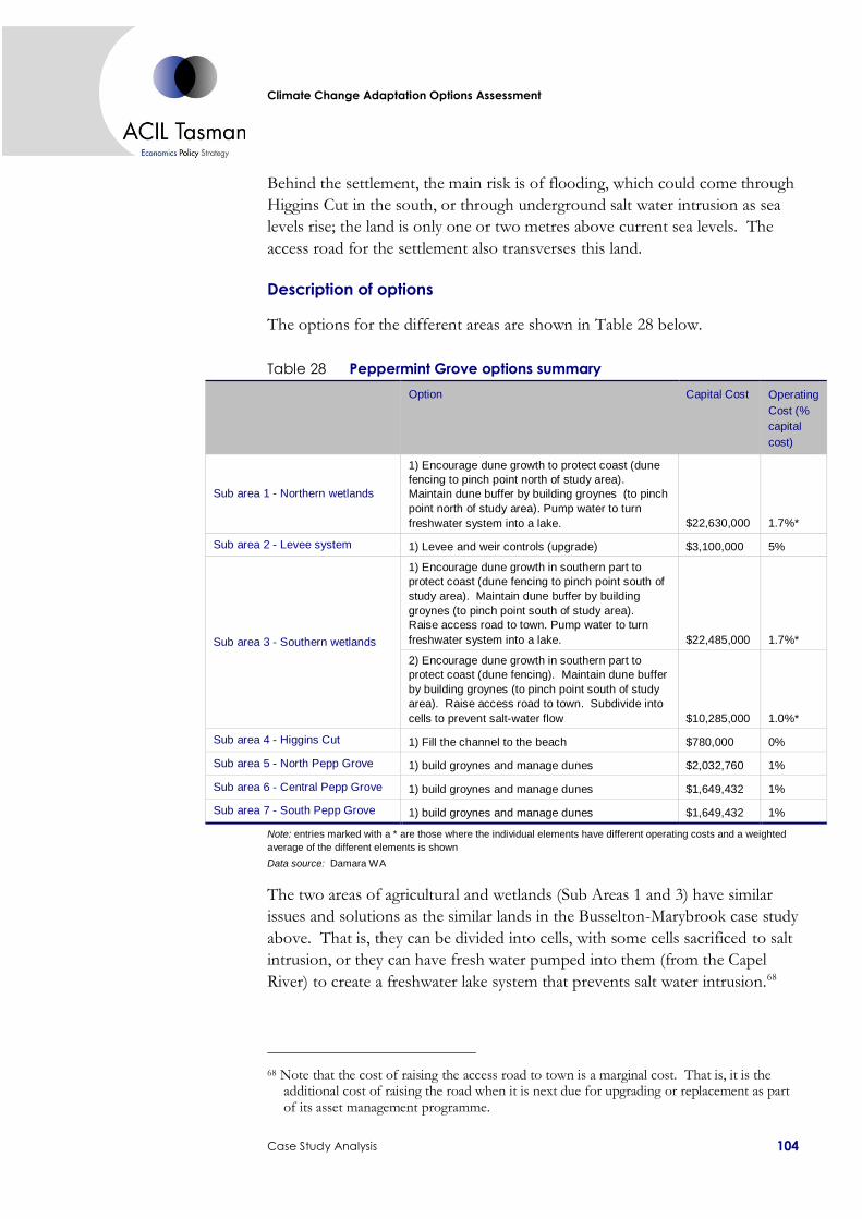
Climate Change Adaptation Options Assessment
Case Study Analysis 104
Behind the settlement, the main risk is of flooding, which could come through
Higgins Cut in the south, or through underground salt water intrusion as sea
levels rise; the land is only one or two metres above current sea levels. The
access road for the settlement also transverses this land.
Description of options
The options for the different areas are shown in Table 28 below.
Table 28 Peppermint Grove options summary
Option Capital Cost Operating
Cost (%
capital
cost)
Sub area 1 - Northern wetlands
1) Encourage dune growth to protect coast (dune
fencing to pinch point north of study area).
Maintain dune buffer by building groynes (to pinch
point north of study area). Pump water to turn
freshwater system into a lake. $22,630,000 1.7%*
Sub area 2 - Levee system 1) Levee and weir controls (upgrade) $3,100,000 5%
Sub area 3 - Southern wetlands
1) Encourage dune growth in southern part to
protect coast (dune fencing to pinch point south of
study area). Maintain dune buffer by building
groynes (to pinch point south of study area).
Raise access road to town. Pump water to turn
freshwater system into a lake. $22,485,000 1.7%*
2) Encourage dune growth in southern part to
protect coast (dune fencing). Maintain dune buffer
by building groynes (to pinch point south of study
area). Raise access road to town. Subdivide into
cells to prevent salt-water flow $10,285,000 1.0%*
Sub area 4 - Higgins Cut 1) Fill the channel to the beach $780,000 0%
Sub area 5 - North Pepp Grove 1) build groynes and manage dunes $2,032,760 1%
Sub area 6 - Central Pepp Grove 1) build groynes and manage dunes $1,649,432 1%
Sub area 7 - South Pepp Grove 1) build groynes and manage dunes $1,649,432 1%
Note: entries marked with a * are those where the individual elements have different operating costs and a weighted
average of the different elements is shown
Data source: Damara WA
The two areas of agricultural and wetlands (Sub Areas 1 and 3) have similar
issues and solutions as the similar lands in the Busselton-Marybrook case study
above. That is, they can be divided into cells, with some cells sacrificed to salt
intrusion, or they can have fresh water pumped into them (from the Capel
River) to create a freshwater lake system that prevents salt water intrusion.68
68 Note that the cost of raising the access road to town is a marginal cost. That is, it is the
additional cost of raising the road when it is next due for upgrading or replacement as part of its asset management programme.

Climate Change Adaptation Options Assessment
Case Study Analysis 105
For this to be successful would require levees and weir controls on the Capel
River in Sub Area 2, and would also require Higgins Cut in Sub Area 4 to be
filled in. If this is not filled in, then there will be a risk of salt water flooding of
Sub Area 3, regardless of whether a freshwater lake system is created or not.
The culvert could be filled in through man-made engineering, or it could be
closed by encouraging a dune to form in the area by building a small groyne.
The former is a short-term and the latter a longer-term option.
The three sub areas within the settlement could be protected by installing
groynes at the appropriate time to hold sand on the beach and prevent erosion.
This would involve beginning in Sub Area 5 in the north of the settlement, and
moving progressively south with new groynes. The dune area would also
require active management by both the Council and by local residents, to
prevent blowouts threatening the viability of the dune systems. Part of this
management would also include relocation of beach-side carparks as the beach
and dune systems change; up to a dozen times during the course of the current
century.
Options and optimal timing results
The viable options for Peppermint Grove Beach are shown in Table 29.
Table 29 Peppermint Grove Beach viable options summary
Sub area Option Capital cost OPEX
Optimal
Year Net benefit
% let expire
scenarios
Sub area 3 -
Southern wetlands 2 $10,285,000 $100,000 2 $5,240,000 1.70%
Sub area 4 - Higgins
Cut 1 $780,000 $- 1 $4,046,000 0.00%
Sub area 5 - North
Pepp Grove 1 $2,032,760 $20,328 5.5 $17,474,000 7.50%
Sub area 6 - Central
Pepp Grove 1 $1,649,432 $16,494 5.5 $14,030,000 5.80%
Sub area 7 - South
Pepp Grove 1 $1,649,432 $16,494 5.5 $10,451,000 2.70%
As with the previous two case studies, there is a division between coastal assets
affected by erosion, and inland assets affected by flooding.
In the case of coastal assets, the solution is the same in each of the three Sub
Area 5,6 and 7; build the groynes in the middle of the fifth year. The net
benefit from doing so is $17, $14 and $10 million respectively. Moreover, the
distribution around this mean is very tight, suggesting a good degree of
confidence around these findings. This is shown in Figure 11.

Climate Change Adaptation Options Assessment
Case Study Analysis 106
There is no existing protection at Peppermint Grove, and by the fifth year of
our time period, 3.5 per cent of each of these coastal assets will have been
eroded. Based on the model results, the community has two choices; either let
the erosion happen or begin building the groynes earlier in a staged process.
Within the sub areas in question, the erosion zone is roughly 375 metres wide,
meaning that 3.5 per cent of it is roughly 13 metres wide. The beach itself,
looking from Google Earth, is 65 metres wide.69 Thus, one option could be to
simply allow some of the beach to disappear; no residential properties would
be in danger.
The other option is to stage the groynes, building one third of the total in Sub
Area 5, and one half in Sub Areas 6 and 7. This would incur a cost of
$680,000 for Sub Area5, and $820,000 in Sub Areas 6 and 7. The optimal time
to do so would not change much from the full option, meaning it would not
save much erosion. However, it would mean that the second stage could be
delayed for 30 years, rather than being done immediately. Thus, costs would
be saved.
69 There is no way of knowing whether the Google Earth image was taken at high or low tide.
Figure 11 Optimal timing distribution for Options 5, 6 and 7 – Peppermint Grove Beach
0
50
100
150
200
250
300
1 5 9
13
17
21
25
29
33
37
41
45
49
53
57
61
65
69
73
77
81
85
89
93
Let
exp
ire
Option Five
0
50
100
150
200
250
1 5 9
13
17
21
25
29
33
37
41
45
49
53
57
61
65
69
73
77
81
85
89
93
Let
exp
ire
Option Six
0
50
100
150
200
250
300
1 5 9
13
17
21
25
29
33
37
41
45
49
53
57
61
65
69
73
77
81
85
89
93
Let
exp
ire
Option Seven

Climate Change Adaptation Options Assessment
Case Study Analysis 107
Box 6 The decision tool and counter-intuitive results
When the model results were presented at the draft report stage, it was noted by PNP
Senior Officers that the rapid timeframe for construction at Peppermint Grove Beach did
not match local understanding of the nature of the erosion threat in the region. We
therefore examined some different assumptions in the model to ascertain what might
have caused these counter-intuitive results.
The real options model works by comparing (in each scenario, and for each option) a
current year outcome with the expectation of an outcome in the following year,
choosing a current year for action if it produces a better outcome than is expected in
the following period. This bilateral comparison is done in each period, and thus there
may be several years in a given scenario where acting in a current year is better than
waiting. In the context of a profit-maximising private-sector operator, the time at which
the difference between the current year outcome and waiting is greatest is the logical
“best” timing for that scenario, if there are several years where current action is preferred
over waiting. However, government is not (necessarily) a profit-maximiser, and is likely to
choose to err on the side of caution. Thus, in all of the modelling in this report, we chose
the first time that a current period was better than an expectation of the future as being
the best time to act. In this way, government does not waste resources by acting too
early, but nor does it run the risk of leaving action too late. The practical upshot of doing
so, however, is that the timing for action is biased towards the present.
For this reason, we re-ran the Peppermint Grove Beach case study, redefining “best” to
mean the time when the difference between a current period and an expectation of the
future is maximised (a “profit-maximising” case) and the last time in the 100-year
timeframe when acting in a current period is better than waiting (a “last-minute”
scenario). In areas subjecting to flooding, such as Sub-Area 3, this resulted in a significant
change in timing; from the second to the 20th year in the case of Sub Area 3. However,
for those areas subject to erosion, changes were minor; from five to nine years in each of
Sub Areas 5, 6 and 7.
Two conclusions might be drawn from this. The first is that the case for immediate action
is very strong, as all three definitions of “best” give broadly similar results. The second is
that the underlying data which are used in the erosion models from the Phase One report
are problematic. We consider the latter to be more likely; in the case of Peppermint
Grove Beach, there are no data on precisely where rock lies along the coast, and the
model in the Phase One report has thus assumed no rock. This has the effect of greatly
amplifying the amount of erosion. For this reason, we would suggest that, in the case of
Peppermint Grove Beach, the first action should be to collect more of the basic data
needed for the engineering models, rather than commencing construction of groynes.
Time limitations restricted a similar exercise for other case study areas, but we suspect the
data availability issue may be more pervasive (see Phase One report for details).
In the case of inland assets, there is no economic justification for protecting
the northern wetlands or the levee, as the cost of doing so is larger than the
reduction in value at risk.70 This is not the case for the southern wetlands, or
70 In this context, it is worth noting that the levee is capable of handling a 50-year flood risk
event, but there are insufficient benefits in upgrading it to handle a 100-year flooding event.

Climate Change Adaptation Options Assessment
Case Study Analysis 108
Higgins Cut. In the former case, this is because the southern wetlands have an
option which does not require pumping water to maintain a freshwater lake
(not available north of the levee) which halves the protection cost. It should
be noted that it would be necessary to install protection at Higgins Cut if the
southern wetlands were worth protecting, because failure to do so would allow
salt water incursion through the cut in times of storm. The model suggests
that both the southern wetlands and Higgins Cut ought to have protecting
applied in the next couple of years, and that doing so would have a net benefit
of between $4 and $5 million. In both cases, the distribution around the mean
optimal year was very tight, suggesting confidence in these results.
Note that, as in Siesta Park-Marybrook, the protection in the southern
wetlands involves the sacrifice of some land and, since the exact position of the
relevant protection measures has not been identified at this stage, we have not
included the cost (or value lost) of this land being affected by salt-incursion. In
this instance, since the net benefits are much lower than was the case in Siesta
Park-Marybrook, this may change the protection decision once the location of
the relevant protection measures are finalised. Note also that the no-protect
decision for the northern wetlands would involve the sacrifice of agricultural
land whose value does not warrant protection in an economic sense. In this
instance, if the community believed the land was worth protecting, it would
need to consider much larger protection costs than in Siesta Park-Marybrook.
Formulation of options pathways
Aside from the potential to stage the construction of groynes to avoid an initial
loss of 3.5 per cent of the land to erosion, there are no pathways for options in
the case study area; each sub area has a single option which is viable.
5.5 Case Study Four: Eaton-Collie River
This case study are covers Eaton, Pelican Point and the southern extremity of
Australind, up to the intersection between Elizabeth St and the Old Coast
Road. It follows the Collie River around the first major bend from the river
mouth and ends roughly at the highway to the East. The case study area
includes the Leschenault Peninsula, and includes three Local Government
areas; the City of Bunbury and the Shires of Harvey and Dardenup. The case
study area has been divided into nine sub sections which are described in Table
30 and shown in Figure 12.
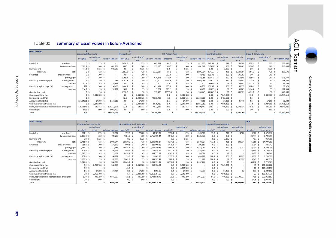
109
Ca
se S
tud
y A
na
lysis
Clim
ate
Ch
an
ge
Ad
ap
tatio
n O
ptio
ns A
ssessm
en
t
Table 30 Summary of asset values in Eaton-Australind
Asset classing 1 2 3 4 5
Leschenault Peninsula Pelican Point Sth Pelican Point Sporting Precinct Bridge & Commercial
area (m2)unit value of
assetvalue of sub-area area (m2)
unit value of
assetvalue of sub-area area (m2)
unit value of
assetvalue of sub-area area (m2)
unit value of
asset
value of sub-
areaarea (m2)
unit value of
assetvalue of sub-area
Roads (m) one lane 0 275$ -$ 2426.6 275$ 667,317$ 2991.5 275$ 822,655$ 747.59 275$ 205,588$ 505.5 275$ 139,007$
two or more lanes 1783.9 360$ 642,204$ 993.5 360$ 357,650$ 2393.5 360$ 861,647$ 2176.28 360$ 783,461$ 2670.6 360$ 961,403$ Railways (m) 417.1 2,325$ 969,758$ 0.0 2,325$ -$ 0.0 2,325$ -$ 0.00 2,325$ -$ 0.0 2,325$ -$
Water (m) retic 0 428$ -$ 2883.8 428$ 1,232,827$ 4424.1 428$ 1,891,304$ 2676.27 428$ 1,144,104$ 1894.0 428$ 809,671$
Sewerage pressure main 0 200$ -$ 0.0 200$ -$ 202.3 200$ 40,459$ 530.92 200$ 106,183$ 0.0 200$ -$
gravity pipes 0 190$ -$ 3265.3 190$ 620,398$ 4522.4 190$ 859,258$ 2183.73 190$ 414,908$ 913.0 190$ 173,463$
Electricity low voltage (m) underground 1.1 150$ 165$ 5247.3 150$ 787,100$ 6801.8 150$ 1,020,269$ 1159.21 150$ 173,881$ 1325.7 150$ 198,856$
overhead 107.5 45$ 4,838$ 0.0 45$ -$ 0.0 45$ -$ 1999.80 45$ 89,991$ 2072.6 45$ 93,268$
Electricity high voltage (m) underground 788 300$ 236,400$ 1404.7 300$ 421,424$ 635.8 300$ 190,750$ 150.86 300$ 45,257$ 124.6 300$ 37,373$
overhead 714.2 55$ 39,281$ 143.0 55$ 7,867$ 989.2 55$ 54,408$ 1005.25 55$ 55,289$ 2054.4 55$ 112,994$
Gas pipelines (m) 0 90$ -$ 6172.2 90$ 555,495$ 10593.8 90$ 953,445$ 4314.69 90$ 388,323$ 4892.2 90$ 440,300$
Commercial land (ha) 0 7,049,300$ -$ 0.0 7,049,300$ -$ 0.0 7,049,300$ -$ 0.00 7,049,300$ -$ 15.1 7,049,300$ 106,535,618$
Residential land (ha) 0 -$ -$ 12.1 6,203,125$ 74,866,492$ 15.9 6,203,125$ 98,324,365$ 0.00 4,462,500$ -$ 2.3 -$ -$
Agricultural land (ha) 124.84592 17,200$ 2,147,350$ 0.0 17,200$ -$ 0.5 17,200$ 7,958$ 1.48 17,200$ 25,440$ 4.2 17,200$ 71,404$
Community infrastructure (ha) 0 7,049,300$ -$ 1.2 7,049,300$ 8,576,469$ 1.9 7,049,300$ 13,051,262$ 0.00 7,049,300$ -$ 14.4 7,049,300$ 101,475,613$
Parks, recreational and conservation areas (ha) 176.22147 620,313$ 109,312,378$ 12.4 620,313$ 7,672,186$ 29.3 620,313$ 18,190,447$ 13.83 446,250$ 6,173,334$ 45.6 446,250$ 20,349,006$
Beaches (m) 3426 900$ 3,083,400$ 0.0 900$ -$ 0.0 900$ -$ 0.00 900$ -$ 0.0 900$ -$
Total 301 116,435,773$ 26 95,765,224$ 47 136,268,229$ 15 9,605,760$ 82 231,397,976$
Asset classing 6 7 8 9 Total
Sth Australind Commercial North Eaton/ South Australind Eaton Proposed Development N
area (m2)
unit value of
asset value of sub-area area (m2)
unit value of
asset value of sub-area area (m2)
unit value of
asset value of sub-area area (m2)
unit value of
asset
value of sub-
area area (m2)
value of case
study area
Roads (m) one lane 361.1 275$ 99,307$ 157.8 275.00$ 43,387.37$ 2,158.4 275$ 593,568$ 17.8 275$ 4,908$ 9,366 2,575,737$
two or more lanes 2,195.3 360$ 790,296$ 7,684.9 360$ 2,766,559.44$ 4,546.0 360$ 1,636,575$ 0.0 360$ -$ 24,444 8,799,795$
Railways (m) 0.0 2,325$ -$ 0.0 2,325$ -$ 0.0 2,325$ -$ 0.0 2,325$ -$ 417 969,758$
Water (m) retic 2,431.0 428$ 1,039,244$ 11,930.0 428$ 5,100,089.87$ 8,374.1 428$ 3,579,937$ 472.8 428$ 202,114$ 35,086 14,999,291$
Sewerage pressure main 921.8 200$ 184,370$ 600.3 200$ 120,069.52$ 1,478.3 200$ 295,660$ 0.0 200$ -$ 3,734 746,742$
gravity pipes 1,644.1 190$ 312,386$ 12,975.5 190$ 2,465,340.87$ 7,490.8 190$ 1,423,250$ 6.5 190$ 1,232$ 33,001 6,270,235$
Electricity low voltage (m) underground 307.9 150$ 46,179$ 489.6 150$ 73,434.79$ 5,511.3 150$ 826,690$ 0.0 150$ -$ 20,844 3,126,576$
overhead 1,636.7 45$ 73,651$ 7,438.4 45$ 334,727.22$ 3,202.1 45$ 144,094$ 0.0 45$ -$ 16,457 740,569$
Electricity high voltage (m) underground 202.8 300$ 60,827$ 39.6 300$ 11,865.86$ 2,132.6 300$ 639,787$ 200.3 300$ 60,095$ 5,679 1,703,779$
overhead 1,505.5 55$ 82,803$ 2,642.3 55$ 145,327.44$ 208.4 55$ 11,462$ 780.5 55$ 42,927$ 10,043 552,358$
Gas pipelines (m) 5,647.8 90$ 508,304$ 18,843.9 90$ 1,695,951.97$ 13,752.9 90$ 1,237,764$ 0.0 90$ -$ 64,218 5,779,583$
Commercial land (ha) 0.2 2,769,700$ 568,048$ 0.1 7,049,300$ 959,356.62$ 0.0 7,049,300$ -$ 0.0 7,049,300$ -$ 15 108,063,022$
Residential land (ha) 7.2 -$ -$ 43.5 -$ -$ 0.0 4,462,500$ -$ 0.0 -$ -$ 81 173,190,858$
Agricultural land (ha) 1.6 17,200$ 27,404$ 0.2 17,200$ 3,096.59$ 0.4 17,200$ 6,337$ 0.0 17,200$ 62$ 133 2,289,052$
Community infrastructure (ha) 0.0 2,769,700$ -$ 5.7 7,049,300$ 40,151,387.00$ 0.0 7,049,300$ -$ 0.0 7,049,300$ -$ 23 163,254,731$
Parks, recreational and conservation areas (ha) 10.9 446,250$ 4,871,227$ 15.1 446,250$ 6,733,979.72$ 20.3 446,250$ 9,061,797$ 84.5 446,250$ 37,698,227$ 408 220,062,582$
Beaches (m) 0.0 900$ -$ 0.0 900$ -$ 0.0 900$ -$ 0.0 900$ -$ 3,426 3,083,400$
Total 20 8,664,046$ 65 60,604,574.28$ 21 19,456,920$ 84 38,009,565$ 661 716,208,067$

Climate Change Adaptation Options Assessment
Case Study Analysis 110
Figure 12 Eaton-Australind case study sub-areas
Sub Area 1 covers the Leschenault Peninsula itself. Sub Area 2 covers the
residential area on Pelican Point, while Sub Area 3 covers the Sanctuary Golf
Course and residential areas between it and the estuary. Sub Are 4 covers
Eaton Sports Ground. Sub Areas 5 and 6 cover the area on the estuary north
of the Collie River up to the southern extremity of Australind. Sub Areas 7
and 8 cover residential areas east of the Clifton Community Reserve on the
north shore of the river and Lions Park on the southern shore. Sub Area 9
covers the riverside land, presently unsettled but slated for development, up to
the first major bend in the Collie River.
Climate change impacts in the Eaton-Collie River case study
The aspect of this case study area which differs from the remainder is the
nature of erosion. According to the climate modelling, the Leschenault
Peninsula will be eroded right at the very end of the case study period, in 2100.
Thus, for the entirety of the case study period, it will offer protection to the
estuary and associated settlements, meaning that all suffer an increase in flood
risk, but no increase in erosion risk. The adaptation options developed below
have been developed with this in mind, and should be considered as such. If
the peninsula begins to erode faster than the model predicts, then there may be
a need to consider measures to alleviate erosion on the peninsula which we do
not consider here. However, it will likely be many decades before such
considerations are needed.
Within the estuary, the main impact is from increased flooding risk. This is
important because many developments, particularly the canal estates in Sub

Climate Change Adaptation Options Assessment
Case Study Analysis 111
Area 2 are low-lying and already subject to flood risk. Moreover, new
development is proposed in several areas within the case study area. The need
to consider action is thus somewhat more urgent than is the case in other case
study areas.
Description of options
The options for the different areas are shown in Table 31 below.

Climate Change Adaptation Options Assessment
Case Study Analysis 112
Table 31 Summary of options in Eaton-Australind
Sub Area Option
Capital Cost Operating
Cost (%
capital cost)
Sub area 2 - Pelican
Point
1) Crest wall. Rock Revetment surrounding Pelican Point. Large seawall
around exposed section of Pelican Point $7,700,000 1.23%*
2) Minimum fill for existing and new houses to raise them (progressive - at
the end of each houses life span). Rock Revetment surrounding Pelican
Point. Large seawall around exposed section of Pelican Point $12,900,000 0.48%*
3) Fully fill existing and new houses (progressive - at the end of each
houses life span). Rock Revetment surrounding Pelican Point. Large
seawall around exposed section of Pelican Point $12,200,000 1.0%
4) Require all new houses to have flood-proofing through raising or other
measures. Rock Revetment surrounding Pelican Point. Large seawall
around exposed section of Pelican Point $17,600,000 0.37%*
Sub area 3 - Sth
Pelican Point
1) Surrounding crest wall. Rock Revetment surrounding Pelican Point. Large
seawall around exposed section of Pelican Point $4,500,000 1.22%*
2) minimum fill for existing and new houses to raise them (progressive - at
the end of each houses lifespan). Rock Revetment surrounding Pelican
Point. Large seawall around exposed section of Pelican Point $8,200,000 0.43%*
3) Fully fill existing and new houses (progressive - at the end of each
houses lifespan). Rock Revetment surrounding Pelican Point. Large seawall
around exposed section of Pelican Point $7,200,000 1.0%
4) Require all new houses to have flood-proofing through raising or other
measures. Rock Revetment surrounding Pelican Point. Large seawall
around exposed section of Pelican Point $12,600,000 0.28%*
Sub area 4 - Sporting
Precinct
1) zone to require future buildings to be flood-proof (assumed potential for 22
lots @ $40,000 per lot) $880,000 0.0%
2) fill oval to raise its level $900,000 0.0%
3) protect oval with a levee $240,000 0.0%
Sub area 5 - Bridge &
Commercial
1) Raise the road and bridge and use road embankment as a levee. Armour
the coastal strip (revetment). Large seawall along coastal strip. $5,310,000 1.0%
2) Preclude development on the coastal side of the road $54,000,000
Sub area 6 - Sth
Australind Commercial
1) Basic foreshore control with low level walling (rock revetment). raise and
fill all the land (progressive - at the end of each houses lifespan). Large
seawall along coastal strip. $9,100,000 1.0%
2) Basic foreshore control with low level walling (rock revetment). Protect
waterside houses with a wall. raise the road and use road embankment as
a levee). Large seawall along coastal strip. $8,700,000 1.05%*
Sub area 7 - North
Eaton/ South
Australind
1) Bank protection and watching brief. Rock revetment along bank.
Manipulate and deepen channels. Modify bridge. $9,00,000 2.18%*
2) Bank protection and watching brief. Rock revetment along bank. Create
an upstream detention basin. $200,800,000 0.51%*
Sub area 8- Eaton
1) Bank protection and watching brief. Rock revetment along bank.
Manipulate and deepen channels. Modify bridge. $9,130,000 2.19%*
2) Bank protection and watching brief. Rock revetment along bank. Create
an upstream detention basin. $201,530,000 0.51%*
Sub area 9 - Proposed
Development N
1) Fill the areas planned for development prior to development. Create an
upstream detention basin. $199,010,000 0.5%*
2) Build levees to protect planned development areas. Create an upstream
detention basin. $198,920,000 0.5%*
Note: entries marked with a * are those where the individual elements have different operating costs and a weighted
average of the different elements is shown
Data source: Damara WA

Climate Change Adaptation Options Assessment
Case Study Analysis 113
As noted above, for the peninsula (Sub Area 1), the fact that erosion is not a
key issue until the end of the period means that a watching brief is the most
appropriate option at this stage.71 However, there may be relatively low cost
things which the Local Government(s) could do in the interim to reduce
erosion. Firstly, they could encourage less erosion by dune fencing.72
Secondly, when Bunbury Harbour is dredged, rather than dumping the sand
out to sea, it could be dumped on the seaward side of the Peninsula, which
would actually be less costly than dumping at sea. This would require
assessment of what contaminants, if any, are in the sand being dredged from
the harbour.
Sub Area 2 is particularly endangered by sea level rise, which would see flood
risk increase substantially, and may render the land uneconomical. Since the
land is already low-lying, a response is required sooner, rather than later, and
there is insufficient time to use a zoning requirement that all new houses be
flood-proofed by raising their foundations with fill or by some other measure.
This means that a cresting wall is required; either with a requirement to fill new
blocks before building houses or without. Sub Area 3 is in a similar situation,
but is slightly less low-lying, and has substantially more houses already
developed.
The main asset in Sub Area 4 is the Eaton Sports Ground, where plans exist
for new spectator facilities. These plans may require re-consideration,
particularly in respect to drainage. The oval itself is in danger of flooding and
is indeed designed to be a floodway.
In Sub Area 5, the main asset is the road and bridge, which can’t be
functionally isolated. This suggests a strategy of raising both to provide a flood
levee, or to armour the coast. The latter would be needed if development
plans in the Clifton Community Reserve go ahead, as this area would not be
protected by a levee at the roadway. A raised road/levee could also be used in
Sub Area 6, but this would not protect the scattering of houses on the water-
side of the Old Coast Road in the north of the sub area. These would need to
be raised (which is difficult for existing houses), or protected with a small
floodwall.
Sub Areas 7 and 8 already have some level of flood control which means that
bank protection and a watching brief may be sufficient. Beyond that, there
may be scope to manipulate the channel in the Collie River to deepen it, or to
71 Some land will be lost, but not enough to prevent the peninsula from performing its role of
protecting the residential and other land in the estuary region. It is, in effect, a “natural” sea wall.
72 This would cost roughly $10,000 per annum.
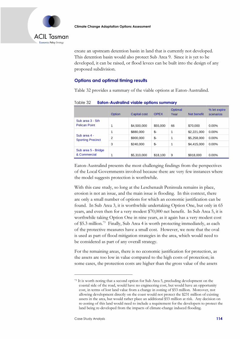
Climate Change Adaptation Options Assessment
Case Study Analysis 114
create an upstream detention basin in land that is currently not developed.
This detention basin would also protect Sub Area 9. Since it is yet to be
developed, it can be raised, or flood levees can be built into the design of any
proposed subdivision.
Options and optimal timing results
Table 32 provides a summary of the viable options at Eaton-Australind.
Table 32 Eaton-Australind viable options summary
Option Capital cost OPEX
Optimal
Year Net benefit
% let expire
scenarios
Sub area 3 - Sth
Pelican Point 1 $4,500,000 $55,000 66 $70,000 0.00%
Sub area 4 -
Sporting Precinct
1 $880,000 $- 1 $2,221,000 0.00%
2 $900,000 $- 1 $5,258,000 0.00%
3 $240,000 $- 1 $4,415,000 0.00%
Sub area 5 - Bridge
& Commercial 1 $5,310,000 $18,100 9 $918,000 0.00%
Eaton-Australind presents the most challenging findings from the perspectives
of the Local Governments involved because there are very few instances where
the model suggests protection is worthwhile.
With this case study, so long at the Leschenault Peninsula remains in place,
erosion is not an issue, and the main issue is flooding. In this context, there
are only a small number of options for which an economic justification can be
found. In Sub Area 3, it is worthwhile undertaking Option One, but only in 65
years, and even then for a very modest $70,000 net benefit. In Sub Area 5, it is
worthwhile taking Option One in nine years, as it again has a very modest cost
of $5.3 million.73 Finally, Sub Area 4 is worth protecting immediately, as each
of the protective measures have a small cost. However, we note that the oval
is used as part of flood mitigation strategies in the area, which would need to
be considered as part of any overall strategy.
For the remaining areas, there is no economic justification for protection, as
the assets are too low in value compared to the high costs of protection; in
some cases, the protection costs are higher than the gross value of the assets
73 It is worth noting that a second option for Sub Area 5, precluding development on the
coastal side of the road, would have no engineering cost, but would have an opportunity cost, in terms of lost land value from a change in zoning of $53 million. Moreover, not allowing development directly on the coast would not protect the $231 million of existing assets in the area, but would rather place an additional $53 million at risk. Any decision on re-zoning of this land would need to include a requirement for the developers to protect the land being re-developed from the impacts of climate-change induced flooding.

Climate Change Adaptation Options Assessment
Case Study Analysis 115
themselves. However, this does not mean that all of the region will be
immediately subject to very high flood risk. In Sub Areas 6,7 and 8, much of
the residential land is sufficiently elevated from sea level that it would not be
affected by flooding, which would instead impact largely on the parks which
are by the shoreline. This means that the actual impacts of non-protection are
likely to be less than might be apparent from a cursory examination of the
model results.
This is not true in Sub Area 2 or in Sub Area 9. Sub Area 9 is not yet
developed, meaning its land value is relatively low. However, the costs of
protection are very high; around $200 million. This means that any plans for
future development would need to ensure that the developer pays this
protection cost up-front to ensure that the allocation of land uses is not
economically inefficient. This may preclude the growth of Eaton into Sub
Area 9.
Sub Area 2 is perhaps the most problematic, as it is already settled, but the
analysis suggests there is insufficient economic justification to protect it.
However, much of the value of Sub Area 2 is due to residential land or the
services to it (power, water, roads etc).74 Moreover, although was, as outside
observers, cannot perceive sufficient economic value to protect the area, those
who live there may have different views. In this instance, since most of the
asset is private land or services to it, there is a prima facie case for residents to
face the full costs of their decision to live in this flood-risk area.
Formulation of options pathways
Since there is very little protection that is economically justified, and only one
option apiece for the Sub Areas where some action is warranted, there are no
pathways per se.
5.6 Lessons learned from case studies
This study in unique in the sense that it is the first time that many of the
aspects involved in undertaking it have been combined. As such, it involved
significant learning curves for both the consulting team and the PNP members.
In this section we provide a brief overview of some lessons learned from the
case studies, which might go on to inform future assessments.
74 About half of the actual area is zoned residential, with the remainder being parkland.
Depending on the value of this parkland to ratepayers outside the Sub Area, there may be scope for partial payment for protection by residents within the Sub Area, and partial payment from the community as a whole. This would be a key issue for the local community in this region to decide.

Climate Change Adaptation Options Assessment
Case Study Analysis 116
Underlying coastal data
As noted in reference to the Peppermint Grove Beach case study area, we have
some concerns in regards to the underlying data which are available for the
engineering assessment undertaken as part of Phase One. The shortcomings
of the available data have been summarised as part of the Phase One Report,
but the key point to make here is that all future decisions about adaptation
ought to be made with the state of the currently available data in mind. This is
particularly important in the context of the model results outlined in this
chapter; we would consider that the current state of information about the
coast is not sufficient to allow for immediate action, as per the model results.
It would rather be more appropriate for resources to be put to better data
collection, followed by a re-assessment of optimal strategies using the same
modelling process as is outlined in this chapter. The most resource intensive
part of strategy formulation from the perspective of the economic modelling
lies in the construction of the model framework. As this has now been done,
the marginal costs of re-running the model using new data (or, indeed, for new
case study areas) are relatively low.
Consideration of areas outside the case study areas
In this report, we do not include consideration of impacts outside the case
study areas. This is because treating these impacts properly would require an
iterative process that is both outside the scope of this study, and not suitable
from a methodological perspective for an initial study such as this which
includes only our assessments, and not direct input from the local community.
However, we can suggest a way forward.
Once this project is complete (subject to the data issues outlined above), and
the findings of our report have been turned, through community consultation
and discussion (taking in non-economic factors as necessary) into proposed
actions in each of the case study areas, this provides a baseline for the next
stage; to consider areas either side of the current case study areas.
In our study, we have begun with an assumption of no existing protection in
place. For the next round of studies, even if no protection has actually been
built, the starting assumption is that the protection mechanisms developed as
part of this project (once endorsed by each local community) ought to form a
baseline for the next study. This would then mean, in a practical sense, that
there would be more erosion in the areas either side of the current case study
areas, and the optimal response to that greater erosion (and flooding) should
be developed through a process like that followed in this paper. To the extent
that the optimal responses for the areas either side of the current case study
areas impose an impact on the case study areas themselves, then consideration
should be made to changing current conclusions about optimal responses in

Climate Change Adaptation Options Assessment
Case Study Analysis 117
the case study areas. There would then be a logical iteration of considering
these impacts on the new areas and so on. The whole process would then be
validated through a community process as we suggest for our study, and there
would be a new baseline for the next assessment, further up and down the
coastline.
In each instance, the movements away from the current case study areas would
continue until the optimal response was not to impose any protection, but
rather to allow the (greater, due to prior protection elsewhere) erosion forecast.
This then forms a natural “break-point” along the coast because allowing
erosion, by definition, halts the process of influence up and down the coast. It
would then be a case of choosing a new collection of case studies (probably
settled areas not included at present) and beginning the same iterative process
again.
The whole process appears time-consuming. However, the next stages of any
such process would be much less resource intensive than this first stage,
because all of the basic elements are in place, and the models have been
developed. Moreover, it is important to work carefully through these iterative
processes to ensure that optimal solutions are reached. Finally, there is still a
great deal of uncertainty associated with future climate change impacts in the
region and a series of future studies, as information is updated (more studies
with the same information are less useful) is likely to lead to lower costs in the
long-run than poorly-timed investment.
Asset specification
In principle, assets can be specified at any level, from an individual house
upwards. However, as noted in Section 5.1, this presents logical flaws and
modelling difficulties when the relevant units are too fine-grained. In our
study, we have matched assets to protection measures, but it may not always be
appropriate to match in exactly this fashion. What is required is not a
mechanistic application of exactly what we have done in this report, but rather
careful consideration of the specific circumstances of the next assessment, in
terms of different asset aggregation methods. Moreover, we would suggest
that it is unlikely that our aggregation choice is perfect, given that this is an
initial study; we would rather expect approaches to improve over time as more
consideration is given to these matters.
Continuation of protection mechanisms
In each instance, the protection mechanisms suggested are sufficient to handle
the predicted erosion or flood risk which warrants their consideration.
However, they are not infinitely lived; some will last to the end of the 100-year

Climate Change Adaptation Options Assessment
Case Study Analysis 118
timeframe, and some will need to be replaced 30 or 40 years after first being
constructed, because this is the asset life for these assets.
We have not included the replacement cost of the assets as they reach the end
of their operational life in our models. The reason for doing so is that most
assets that have a lifespan which ends prior to 2100 only end their lives a few
years before this date, and the summary of the net benefits of the next asset is
somewhat unrealistic because the erosion series only goes as far as 2100.
Extending the model out to infinity would change both the cost and the net
benefit, but it would not change the decision of when the first time to invest is,
nor, since each asset lasts until its design life ends, would it change the timing
of subsequent replacements of each asset. The value of the change in benefit
is impossible to forecast with any accuracy, but since benefits are expressed in
net present value terms, is likely to be small. As a rough rule of thumb, the
present cost of each subsequent protection measure replacement is roughly a
third of the previous replacement, if the protection measures last 40 years (and
the discount rate is three per cent), which would mean that the present value of
the costs involved for keeping each protection measure in place forever would
be 50 per cent above the cost of establishing it in the first instance.
Mechanistic use of models
One way of moving from options to option pathways is to use a model to test
all possible combinations. However, as we note with our “third row of houses”
problem noted above, this is unlikely to be optimal, and it is far more likely
that human intervention and consideration are required. The same is true of
the assessment of the options themselves. The first set of results that came out
of our modelling are not the same as the final set, and there were various issues
which needed to be considered to question what the results were actually
saying and why. Part of this was because the model was in the development
stage. However, any model is only as good as what goes into it, and it is
usually the case that model results need to be interpreted carefully, rather than
blindly accepted. This requires a degree of familiarity with the way in which
the model(s) work, and not treatment of them as a black box.
Institutional knowledge
As noted above, this project involved a great deal of new learning for all
concerned. Moreover, the process has only just begun; turning the findings of
this report into realistic actions for each local community will present its own
set of fresh challenges. Through this process, a considerable deal of
institutional knowledge has been developed. The tasks at hand are not simple,
and the existing knowledge base within the State and Local Governments is
not ideally suited to doing this kind of work; even down to very simple issues

Climate Change Adaptation Options Assessment
Case Study Analysis 119
like being able to produce maps of assets across local government boundaries.
This means that, if all that happens out of this process is that a report sits on a
shelf, the next group of councils (and the PNP partners themselves at the next
stage of the process; we have not “solved” climate change adaptation for the
region by any means) will face exactly the same learning curve. We therefore
consider it crucial that resources be put to maintaining the PNP structure and
institutional knowledge, as well as sharing that knowledge with other local
government bodies elsewhere in the State. In this manner, vital information
will not be lost, and the project will have a much greater lasting value to the
community.

Climate Change Adaptation Options Assessment
Conclusions and Steps Forward 120
6 Conclusions and Steps Forward
This project has examined the issue of how to formulate options and make
decisions in regards to adaptation to climate change. In this respect, the report
has two key roles; firstly to develop and implement approaches to assist in
strategic decisions pertaining to climate change adaptation, and secondly to
provide a reference or guidebook for future assessment. For this reason, it
includes extensive discussion of economic technique, and underlying economic
ideas, to assist decision-makers less familiar with economics.
The report comprises three main parts:
• A background discussion around the key economic concepts of value and
methods of valuation.
• A region-wide assessment intended to provide an overall appreciation of
the resource cost of climate change adaptation in the South West of WA.
• A detailed account of four case study investigations of adaptation strategy
in four case study areas in the South West of WA.
The first element focuses on ideas and techniques. Since adaptation responses
often involve assets that are not traded in marketplaces, such as parks and
reserves, and since the valuation of these assets presents unique decision-
makers, much of the focus of the discussion is on the valuation of non-market
assets. In many cases, such assets are valued according to “benchmark” values,
drawn from other studies and/or used by many decision-makers without any
real consideration about where these numbers come from and whether they are
in fact applicable. This kind of “paint-by-numbers” approach to economics is
not only damaging in that it can lead to poor, poorly-informed decisions, but
also because it invests economics with a great deal more objectivity and
“science” than it actually possesses, and pushes other decision-making
techniques, that are often more effective, to the background. For this reason,
we devote extensive space to critiquing economic valuation and valuation
techniques, putting economic methodologies in what we consider to be a more
appropriate context in decision-making. As economists, we consider that, if
this section of the report does little more than cast doubt on “paint-by
numbers” economic assessment and contributes to decision-makers
considering a wider range of inputs to decisions than consultants’ benefit-cost
analyses, it will have been successful.
The section on ideas and techniques also introduces two concepts that we have
found useful in our consideration of adaptation strategies. The first is the
notion of “value at risk”. Consider the case of Sydney Harbour, affected by
climate change. One approach to designing strategies could be to begin with
an investigation of what the harbour is worth, and whether it is worth saving.

Climate Change Adaptation Options Assessment
Conclusions and Steps Forward 121
However, this is not only very difficult, but, worse, it is pointless for decision-
makers. Instead, one needs to look at what might happen in Sydney Harbour
if sea levels rose; some housing would be affected, along with some transport
links, but many of the aspects of the harbour which gives it value (like its
views) would be largely unaffected. A value at risk approach looks at what
climate change might do to an asset, and the costs of society from these
impacts. It not only has a spatial element (the various parts of Sydney Harbour
above) but also a temporal element; a house that is not affected by erosion for
50 years still has value by virtue of being habitable for several decades before it
must be abandoned, for example. In general, value at risk is much simpler to
establish than value (we present some simple mathematical equations) and also
provides a much more robust basis for decision-making.
The second notion we term “decision-relevant analysis”. As noted above,
benchmark values usually make for very poor economics, but, used within the
correct context, they can still support robust decision-making. For example,
consider a local government officer who needs to make a decision about
protecting a beach from erosion. Surveying the local community is expensive,
but accessing work undertaken in Melbourne suggests that the beach might be
worth $1 million, based on the value of roughly comparable beaches in
Melbourne. This estimate might have an error band around it which renders it
useless as a valuation tool (or even an estimate of value at risk), but if the only
way to protect the beach is to spend $50 million on off-shore reefs, then even
this highly imperfect estimate of value (at risk) might be good enough to make
a decision not to save the beach; it is “decision-relevant” information. The
same would be true if the numbers were reversed.
The decision-relevant approach is useful because it allows local government
officers to make use of scarce resources more efficiently. For example, an
initial assessment, based on imperfect benchmarks could be used to make
decisions on all the “obvious” cases; say those where the ratio between value at
risk and costs of protection was either greater than five to one or less than one
to five. Our experience in this project suggests that many if not most assets
fall into this category. For these assets, the benchmark is decision-relevant.
For those that remain (between one to five and five to one), the officer can
then consider more detailed assessments, which take into consideration local
factors. For those where the benefits and costs are very closely aligned, the
local government in question could devote yet more resources to detailed
discussions with the community; at each level, the decision-relevant
information changes. The benefit of this approach is in the resources that are
saved; rather than doing detailed work on all assets in the community (or the
ones that people say are most important), the local government in question can
focus its resources on the ones where it is hardest for an outside observer
using generalist information to come to the “correct” decision.

Climate Change Adaptation Options Assessment
Conclusions and Steps Forward 122
The second part of the project involves developing an understanding of the
overall resource cost of adaption within the region as a whole. This does not
mean the cost of “saving” every inch of coastline, but rather the cost, in
general terms, of protecting those assets where the value at risk exceeds the
cost of protection, and engaging in a strategic retreat elsewhere. The aim of
the report is not to design strategy, which we consider ought to be developed
at a more micro level, but is rather to highlight likely resource cost.
Since the work is being undertaken at a regional level, it involves a number of
key abstractions and simplifications from what would be expected in a more
detailed, micro-level assessment. The first such simplification is on the assets
themselves. These are classed into several classes (houses, roads, parks etc;
based on the classification in databases held by the Department of Planning)
and then a single, representative value is applied to all assets in a given class.
The second key simplification is that the location of the assets is not
considered; we consider residential properties in general, rather than where
they are located. This means that we assess the merit of protecting each asset
class in its own right, without considering whether a protection mechanism
along the shoreline would protect different types of assets behind it, including
those which would not merit protection in their own right. Finally, the
investigation examines assets at four snapshots in time, rather than as a
continuous series over time.
At the regional level, erosion is a far more pervasive issue than flooding; while
around 800 hectares of residential land would be subject to an increase in
flooding risk (from one in 500 to one in 100), a strip roughly 200 metres wide
is at risk from erosion along the whole extent of the coastline. The value at
risk of the affected assets along this section of coastline is approximately $1.2
billion. Of these, a little more than $1.1 billion of assets are worth saving, as a
cost of around $120 million, giving a benefit cost ratio of approximately nine
to one.
A corollary of this finding is that around $80 million in assets are not worth
saving. However, in land area terms, this equates to around 80 per cent of the
affected region. The basic finding of the model is that the highly-valued
settlements along the coast ought to be saved, delivering a benefit cost ratio of
nine to one, while the much lower-values agricultural land and nature reserves,
delivering a benefit cost ratio of only 15 per cent, ought not to be protected.
In practice, where this farmland and/or nature reserve sits behind more
valuable settled areas, the protection afforded to the settled areas will also
affect the less valuable land (though not from incursion of salt-water flooding).
However, in many instances, local farming communities will need to consider
the value of protection very carefully, given its costs.

Climate Change Adaptation Options Assessment
Conclusions and Steps Forward 123
Flooding is, as noted above, less of an issue at a regional level than erosion.
The 800 affected hectares of residential (primarily) land would be optimally
protected by requiring all new homes in the affected areas to be built on pads
450mm thick, at a cost (marginal, at time of building, of $12,000 per house).
The timeframe of the increase in risk is such that, were this requirement to be
imposed now, few existing houses would still be standing when the flood risk
changes. The cost, in net present value terms, of this requirement would be
$39 million.
The third part of the report is the four case studies, assessed at a much more
detailed level intended to inform strategy for the relevant local governments.
Here again, there is a strong emphasis on the “how to” side, and a detailed
description of methodology. Unlike the region-wide analysis, the case studies
have a temporal (that is, effects occur on an annual basis) and a spatial element;
we differentiate between locations, and consider assets together than would be
protected together.
There are four case study areas; in Mandurah, Eaton-Australind, Peppermint
Grove Beach and Siesta Park-Marybrook. The areas, and the different feasible
adaptation measures, were chosen in conjunction with the PNP Partners,
whose assistance in this regard is greatly appreciated. In most instances, with
the exception of Eaton-Australind, there were viable options that represented
significant net benefits from protection.
The results of the assessment are perhaps less important than the means by
which the assessment was undertaken. A common way of assessing
infrastructure investments, whether they be as part of climate change
adaptation measures or not is to use benefit cost analysis. However, benefit
cost analysis is rarely suitable in this context. In the first instance, the timing of
the investment has to be found by some other means; a benefit cost
assessment will not indicate the optimal timing of investment. Secondly, a
benefit cost assessment cannot suitably address uncertainty, which means the
results of such an analysis are not robust to changes in circumstance.
For this reason, we made use of real options analysis, in particular an approach
developed by Longstaff & Schwarz (2001), which is able to encapsulate
numerous sources of uncertainty in a mathematically tractable fashion. Real
options analysis has its origins in the study of financial options, and is a special
case of contingent claims analysis. It takes into consideration the fact that a
decision-maker does not need to act today, but instead can wait before
investing. This ability to wait has a value to the decision-maker in the case of
irreversible investments. It also brings uncertainty about future outcomes into
the centre of the analysis, delivering answers that show the optimal time to
implement a response that is the most robust over the range of feasible
situations likely to be faced.

Climate Change Adaptation Options Assessment
Conclusions and Steps Forward 124
Our approach works in practice by taking the models used to generate climate
change outcomes in the Phase One report, and using them to derive several
thousand future scenarios which could be faced by each of the assets in each of
the case study areas. The model then chooses the best time to invest in each
one of these scenarios through a process of backwards induction, and the
optimal response in an overall sense is then the average (the approach also
shows the distribution around the average, allowing for statistical inference to
be applied) of the optimal responses over all of the scenarios chosen. The
approach shows both the value of this optimal response, and when it ought to
be applied. It can also be used to bring together several options in a
“pathway” which represents the best combinations of these individual options.
Real options is widely used by decision-makers in the private sector,
particularly mining companies seeking to value leases which confer the right,
but not the obligation, to mine for minerals. However, there has been only
very limited application of the approach in climate change assessment, despite
its utility in handling issues of timing and uncertainty which are so germane to
the field. To our knowledge, this paper represents the first application of the
particular methodology of Longstaff & Schwarz (2001). However, we hope
that the exposition of our approach in the report does not mean it is the last.
Climate Change Adaptation Options Assessment
Bibliography 125
7 Bibliography
Acemoglu, DA & Robinson, JA, 2002, “The Political Economy of the Kuznets
Curve”, Review of Development Economics, 6(2), 183-203
AECOM, 2010, Coastal Inundation at Narrabeen Lagoon: Optimising adaptation
investment, Report prepared for the Department of Climate Change.
Arrow, KJ (1950), “A Difficulty in the Concept of Social Welfare” Journal of
Political Economy 58(4) 328-46.
Arrow, KJ, 1995, Intergenerational Equity and the Rate of Discount in Long-Term
Social Investment, Paper presented at the IEA World Congress, available from:
www.econ.stanford.edu/faculty/workp/swp97005.pdf.
Arrow, KJ, Cline, W, Maler, KG, Munasinghe, M, Squitieri, R & Stiglitz J,
1996, “Intertemporal Equity, Discounting, and Economic Efficiency”, in
Bruce, JP, Lee, H & Haites EF (eds) Climate Change 1995: Economic and Social
Dimensions of Climate Change, Cambridge; New York and Melbourne:
Cambridge University Press for the IPCC.
Barbier, E, 2011, “Pricing Nature”, Annual Review of Resource Economics, 3, 337-
53.
Baumol, W, 1968, “On the Social Rate of Discount,” American Economic Review,
58(4), 788–802.
Bazelon, C & Smetters, K, 1999, “Discounting in the Washington DC
Beltway”, Journal of Economic Perspectives, 13(4), 213-28.
Bin, O & Polasky, S, 2004, “Effects of Flood Hazards on Property Values:
Evidence before and after Hurricane Floyd”, Land Economics, 80(4), 490-500
Black, F & Scholes, M, 1973, “The Pricing of Options and Corporate
Liabilities”, Journal of Political Economy, 81(3) 637-54.
Boardman, AE, Moore, MA & Vining, AR, 2010, “The Social Discount Rate
for Canada Based on Future Growth in Consumption”, Canadian Public Policy,
36(3), 323-41.
Bockstael, NE & Freeman, AM, 2005, “ Welfare Theory and Valuation”, in
Maler, KG & Vincent, JR (eds) Handbook of Environmental Economics, Vol 2,
Amsterdam: Elsevier North-Holland, 518-70

Climate Change Adaptation Options Assessment
Bibliography 126
Bureau of Infrastructure, Transport and Regional Economics (BITRE), 1999,
Facts and Furphies of Cost Benefit Analysis, available from
www.bitre.gov.au/publications/1999/report_100.aspx.
Bureau of Transport and Regional Economics (BTRE), 2005, Risk in Cost–
Benefit Analysis, BTRE Report 110, available from
www.btre.gov.au/info.aspx?NodeId=58&ResourceId=25.
Carson, RT & Haneman, WM, 2005, “Contingent Valuation”, in Maler, KG &
Vincent, JR (eds) Handbook of Environmental Economics, Vol 2, Amsterdam:
Elsevier North-Holland, 821-936.
Cass, D, 1965, “Optimum Growth in an Aggregative Model of Capital
Accumulation”, Review of Economic Studies, 32(3), 233–40.
Coase, RH, 1960, “The Problem of Social Cost,” Journal of Law and Economics, 3
1–44.
Colombo, S, Calatrava-Requena, J & Hanley, N, 2007, “Testing Choice
Experiment for Benefit Transfer with Preference Heterogeneity”, American
Journal of Agricultural Economics, 89(1), 135-51.
Committee on Assessing and Valuing the Services of Aquatic and Related
Terrestrial Ecosystems, National Research Council, 2004, Valuing Ecosystem
Services: Toward Better Environmental Decision-Making, Washington: National
Academies Press, available from www.nap.edu/catalog/11139.html.
Costanza, R, d’Arge, R, de Groot, R, Farber, S, Grasso, M, Hannon, B,
Limburg, K, Naeem, S, O’Neill, R, Paruelo, J, Raskin, R, Sutton, P & van den
Belt, M, 1997, “The Value of the World’s Ecosystem Services”, Nature, 387,
253-60.
Cox, JC, Ross, SA & Rubinstein, M, 1979, “Option Pricing: A simplified
approach”, Journal of Financial Economics, 7 229-63.
Dasgupta, P, & Maskin, E 2005, “Uncertainty and Hyperbolic Discounting”,
American Economic Review, 95(4), 1290–99.
Dasgupta, P, 2005, “Three Conceptions of Intergenerational Justice”, in
Lillehammer H &. Mellor DH (eds) Ramsey’s Legacy, Oxford: Oxford
University Press, Clarendon Press.
Dasgupta, P, 2007, “Commentary: The Stern Review’s Economics of Climate
Change,” National Institute Economic Review, 199, 4-7.
Dasgupta, P, 2008, “Discounting Climate Change”, Journal of Risk and
Uncertainty, 37(2-3), 141-69.

Climate Change Adaptation Options Assessment
Bibliography 127
Dasgupta, P, Mäler KG & Barrett, S, 2000, Intergeneration Equity, Social Discount
Rates and Global Warming, available from:
www.econ.cam.ac.uk/faculty/dasgupta/pub07/climate.pdf.
Dixit AK & Pindyck, RS, 1994, Investment Under Uncertainty, Princeton
University Press, New Jersey.
Dixit, A & Williamson, A, 1989, Risk-Adjusted Rates of Return for Project Appraisal,
World Bank WPS 290.
Dobes, L, 2008, “Getting Real about Adapting to Climate Change: Using “Real
Options” to Address the Uncertainties”, Agenda, 15(3), 55-72.
Ehrlich, P& Ehrlich, A, 1996, Betrayal of Science and Reason¸ Washington DC:
Island Press.
Evans, DJ & Sezer, H, 2004, “Social Discount Rates for Six Major Countries”,
Applied Economics Letters, 11, 557-60.
Evans, DJ, 2005, “The Elasticity of Marginal Utility of Consumption:
Estimates for 20 OECD Countries”, Fiscal Studies, 26(2), 197–224.
Feldstein, MS, 1964, “Cost-Benefit Analysis and Investment in the Public
Sector”, Public Administration, 42(4), 351–72.
Feldstein, MS, 1965, “The Derivation of Social Time Preference Rates”, Kyklos,
18(2), 277-87.
Grant, S & Quiggin, J, 2003, “Public Investment and the Risk Premium for
Equity”, Economica, 70, 1-18.
Hallstrom, D & Smith, VK, 2005, “Market Responses to Hurricanes”, Journal of
Environmental Economics and Management, 50(3), 541-61.
Harberger, A, 1972, Project Evaluation: Collected Papers, Chicago: University of
Chicago Press.
Harrison, M, 2010, Valuing the Future: The social discount rate in cost benefit analysis,
Productivity Commission Visiting Researcher Paper, April 2010, available
from www.pc.gov.au/research/visiting-researcher/cost-benefit-discount.
Heal, GM, 1997, “Discounting and Climate Change”, Climate Change, 37, 335–
343.
Heal, GM, 1998, Valuing the Future: Economic Theory and Sustainability, New York:
Columbia University Press.
Henn, L, Douglas, N & Sloan, K, 2011, “Surveying Sydney Rail Commuters’
Willingness to Change Travel Time”, Australasian Transport Research Forum

Climate Change Adaptation Options Assessment
Bibliography 128
2011, Adelaide, Australia, September 2011, available from
www.atrf11.unisa.edu.au/PaperListing.aspx.
Hirshleifer, J, 1965, “Investment Decisions under Uncertainty: Choice-
Theoretic Approaches”, Quarterly Journal of Economics, 79, 71–79.
Hunter, G, 2003, “Incomplete Markets and Hyperbolic Discounting”, The
Journal of Risk and Insurance, 70(1), 97-109.
Hunter, JR, 2006, Testimony before the Committee on Banking, Housing and Urban
Affairs of the United States Senate Regarding Proposals to Reform the National Flood
Insurance Program.
Karl, T R et al, 2008 Weather and Climate Extremes in a Changing Climate, U.S.
Climate Change Science Program Synthesis and Assessment Product 3.3,
June 2008.
Koopmans, TC, 1960, “Stationary Ordinal Utility and Impatience”, Econometrica
28(2), 287-309.
Koopmans, TC, 1965, “On the Concept of Optimal Economic Growth”,
Academiae Scientiarum Scripta Varia, 28(1), 225–87.
Lander, DM & Pinches, GE, 1998, “Challenges to the Practical
Implementation os Modeling and Valuing Real Options”, Quarterly Review of
Economics and Finance, 38(sp) 537-67.
Lind, RC & Arrow, KJ, 1970, “Uncertainty and the Evaluation of Public
Investment Decisions”, American Economic Review, 60(3), 364-78.
Lind, RC, 1982, “A Primer on the Major Issues Relating to the Discount Rate
for Evaluating National Energy Options”, in Lind RC (ed.). Discounting for
Time and Risk in Energy Policy, Washington, DC: Resources for the Future, Inc.
Lind, RC, 1990, “Reassessing the Government's Discount Rate Policy in Light
of New Theory and Data in a World Economy with High Degree of Capital
Mobility”, Journal of Environmental Economics and Management, 18, S8- 28.
Little, IMD & Mirrlees JA, 1974, Project Appraisal and Planning for the Developing
Countries, London: Heinemann Educational Books.
Liu, S, Costanza, R, Farber, S & Troy, A, 2010, “Valuing Ecosystem Services:
Theory, practice, and the need for a transdisciplinary synthesis”, Annals of the
New York Academy of Sciences, 1185, 54-78.
Longstaff FA & Schwartz, ES, 2001, “Valuing American Options by
Simulation: A Simple Least-Squares Approach”, Review of Financial Studies,
14(1) 113-47.

Climate Change Adaptation Options Assessment
Bibliography 129
Lopez, H, 2008, The Social Discount Rate: Estimates for nine Latin American countries,
World Bank Policy Research Working Paper 4369, available from
http://elibrary.worldbank.org/content/workingpaper/10.1596/1813-9450-
4639.
Manne, A. S. 1995, “The Rate of Time Preference: Implications for the
greenhouse debate”, Energy Policy 23, 391-94.
McConnell, KE & Bockstael, NE, 2005, “Valuing the Environment as a Factor
of Production”, in Maler, KG & Vincent, JR (eds) Handbook of Environmental
Economics, Vol 2, Amsterdam: Elsevier North-Holland, 622-69.
Merton, RC, 1973, “Theory of Rational Asset Pricing”, Bell Journal of Economics
and Management Science, 4(1) 141-83
Merton, RC, 2001, “Applications of Options Pricing Theory: Twenty-five years
later”, in Schwartz ES & L Trigeorgis (eds) Real Options and Investment Under
Uncertainty, MIT Press, Cambridge Massachusetts, 623-32.
Meyers, SC, 1977, “Determinants of Corporate Borrowing”, Journal of Financial
Economics, 5(2) 147-175.
Mills, E, Roth RJ, & Lecomte, E, 2006, “Availability and Affordability of
Insurance Under Climate Change: A Growing Challenge for the US”, Journal
of Insurance Regulation, 25(2), 109-49, available from:
http://insurance.lbl.gov/availability-affordability.html.
Mills, E. 2005, “Insurance in a Climate of Change”, Science, 309(5737), 1040-44.
Morrison, M, Bennet, J Blamey, R & Louviere, J, 2002, “Choice Modelling and
Tests of Benefit Transfer:, American Journal of Agricultural Economics, 84(1), 161-
70.
Nash, C, 2010, “Current Debates on the Cost Benefit Analysis of Transport
Projects in Great Britain”, Cuadernos Económicos De Ice, 80, 67-81.
Nordhaus, WD, 1994, Managing the Global Commons: The economics of climate change,
Cambridge, Mass,: MIT Press.
Nordhaus, WD, 2007, “A Review of the Stern Review on the Economics of Climate
Change”, Journal of Economic Literature, 45, 686–702.
Nozick, R, 1974, Anarchy, State and Utopia, Basic Books: New York.
Ostrom, E, 1990, Governing the Commons: The evolution of institutions for collective
action, Cambrige Uni Press: New York.

Climate Change Adaptation Options Assessment
Bibliography 130
Palmquist, RB, 2005, “Property Value Models”, in Maler, KG & Vincent, JR
(eds) Handbook of Environmental Economics, Vol 2, Amsterdam: Elsevier North-
Holland, 764-819.
Phaneuf, DJ & Smith, KV, 2005, “Recreation Demand Models”, in Maler, KG
& Vincent, JR (eds) Handbook of Environmental Economics, Vol 2, Amsterdam:
Elsevier North-Holland, 672-761.
Pimental, D, Wilson, C, McCullum, C, Huang, R, Dwen, P, Flack, J, Tran, Q,
Saltman, T & Cliff, B, 1997, “Economic and Environmental Benefits of
Biodiversity”, Bioscience, 47, 747-57.
Ramsey, FP, 1928, “A Mathematical Theory of Saving”, Economic Journal,
38(152), 543-59.
Rawls, J, 1971 A Theory of Justice, Revised version published in 1999 by Harvard
University Press: Cambridge Mass.
Rawls, J, 1971, A Theory of Justice, Cambridge Mass: Harvard University Press.
Samuelson, PA, 1954, "The Pure Theory of Public Expenditure". Review of
Economics and Statistics 36 (4): 387–389.
Schumpeter, JA, 1954, History of Economic Analysis, New York, Oxford
University Press
Sen, A, 2009, The Idea of Justice, Harvard University Press: Cambridge, Mass
Shane, F, Loewenstein, G & O'Donoghue, T, 2002, “Time Discounting and
Time Preference: A critical review”, Journal of Economic Literature, 40(2): 351–
401.
Shogren, JF, 2005, “Experimental Methods and Valuation”, in Maler, KG &
Vincent, JR (eds) Handbook of Environmental Economics, Vol 2, Amsterdam:
Elsevier North-Holland, 970-1027.
Spackman, M, 2004, “Time Discounting and of the Cost of Capital in
Government”, Fiscal Studies, 25(4), 467-518.
Stern, HN, 1977, “Welfare Weights and the Elasticity of Marginal Utility of
Income,” in Artis, M & Norbay, R (eds), Proceedings of the Annual Conference of
the Association of University Teachers of Economics, Oxford: Blackwell.
Stern, HN, Peters, S, Bakhshi, V, Bowen, A, Cameron, C, Catovsky, S, Crane,
D, Cruickshank, S, Dietz, S, Edmonson, N, Garbett, SL, Hamid, L, Hoffman,
G, Ingram, D, Jones, B, Patmore, N, Radcliffe, H, Sathiyarajah, R, Stock, M,
Taylor, C, Vernon, T, Wanjie, H & Zenghelis D, 2006,. Stern Review: The
Economics of Climate Change, London: HM Treasury.
Climate Change Adaptation Options Assessment
Bibliography 131
Sumaila, UR & Walters, C, 2005, “Intergenerational Discounting: A new
intuitive approach”, Ecological Economics, 52, 135– 42.
United Nations Research Institute for Social Development (UNRISD), 2010,
Combating Poverty and Inequality: Structural Change, Social Policy and Politics,
Available from www.unrisd.org/publications/cpi
Van Ewijk, C & Tang, PJG, 2003, “How to Price the Risk of Public
Investment?”, De Economist, 151(3), 317-28.
Varian, H, 1992, Microeconomic Analysis: Third Edition, Norton: New York.
Watson, K, 1992, “The Social Discount Rate”, Canadian Journal of Program
Evaluation, 7(1), 99-118.
Weitzman, ML, 2001, “Gamma Discounting”, American Economic Review 91,
261-71.
Weitzman, ML, 2007, “A Review of the Stern Review on the Economics of
Climate Change” Journal of Economic Literature, 45(3), 703–724.
Climate Change Adaptation Options Assessment
Bibliography 132
Appendix A Cost of Insurance and Climate Change
Managing society’s exposure to events associated with climate change is
essentially an exercise in risk management. This can involve physical measures
(such as building flood protection infrastructure), regulatory measures (such as
land planning and building codes), emergency response measures and financial
instruments (such as creating a contingency fund or insuring against risk of
extreme events). This section examines how the latter can help society manage
the risks associated with climate change and how the insurance industry
responds to changes in the risk exposure to extreme events.
A.1 Community response to changes in insurance
The insurance industry can exert a strong influence on private firms and
citizens to take actions or adopt measures to manage future risk exposure. For
example, as insurance premiums on coastal properties at risk of flooding due to
sea level rise increase this will have an influence on decisions on where to build
or even whether to build at all.
Indeed, houses in an area with high probability of damage due to weather
events should sell for less than comparable houses in an area with a lower risk
of damage. Researchers in the US have examined property values after and
before extreme weather events to judge people’s perceptions of risk on
property values. One such study (Halstrom & Smith, 2005) examined property
values before and after hurricane Andrew in Lee County, Florida. They found
that property values in special flood hazard areas of Lee County declined by 19
per cent after hurricane Andrew.
The findings agreed with those of a similar study that examined housing values
in a flood plain in North Carolina (Bin & Polasky, 2004). It found that prices
declined significantly after hurricane Floyd, compared to houses not seen as at
risk. For the average house, the decline in price exceeded the present value of
premiums for flood insurance, suggesting that the latter could be regarded as a
lower bound to the value of avoiding floods.
Insurance can of course also have the perverse incentive of encouraging more
risky behaviour. A more common example is sometimes referred to as the safe
development paradox. This occurs when perceived increases in safety (for
example, due to the construction of sea walls) induces more building than
might otherwise be the case (such as in areas considered safe due to the
protection provided by a sea wall), leading to increased losses if a major storm
surge overwhelms the sea wall (Karl, et al, 2008).

Climate Change Adaptation Options Assessment
Bibliography 133
A.2 Insurance industry response to climate change
The insurance industry has for some time been at the forefront of private
sector firms expressing concerns regarding the impacts of climate change. This
is not surprising given that insurance claims for damage from extreme weather
events have a direct impact on insurance companies’ bottom lines. Indeed, as
the world’s largest industry the implications of rising disaster losses on insurers
are as important as defining the industry’s role in furthering understanding of
the problem and advancing loss prevention solutions.75
To date, efforts to quantify trends in losses caused by climate change impacts
have tended to be based on insured loss data or on total loss (insured plus non-
insured losses) estimates developed by insurers. However, the details of the
insured losses are seen as commercially sensitive and therefore only aggregated
information tends to be available. The relationship between insured losses and
total losses will vary as a function of the nature of the extreme event, building
codes, the cost of insurance, insurance take up rates, and other factors (Mills,
2005).76
However, it is clear that the trend in insured losses is upwards. As one
researcher noted (ibid):
“weather-related [insured] losses in recent years have been trending upward
much faster than population, inflation, or insurance penetration, and faster
than non-weather-related events”
As losses have mounted the insurance has responded by increasing the
premium paid by businesses and individuals. There has also been pressure on
governments to step in as the ‘insurer of last resort’ when the private sector is
either unwilling to provide an insurance product or the cost of that product is
too high. Where this occurs, the individual losses for victims of major events
can decrease as society as a whole absorbs a portion of their losses either
through disaster relief and or government insurance schemes.
Government insurance schemes transfer the risk from the private sector to the
public sector. This can expose governments to considerable costs. For
example, Hurricane Katrina exhausted the federally backed US National Flood
Insurance Program, which had to borrow $20.8 billion from the Government
to fund the Katrina residential flood claims (Hunter, 2006). However,
75 The insurance industry would be the third largest country if its $3.2 trillion in yearly
revenues were compared with national gross domestic products (GDPs).
76 The US National Hurricane Center generally assumes that total losses are twice insured loss estimates. However, this relationship will not necessarily be true in other countries or for other loss causing events.

Climate Change Adaptation Options Assessment
Bibliography 134
governments that are trying to balance their budgets find that paying large
numbers of claims make doing so much more difficult and, not surprisingly,
they will seek to limit their risk exposure in different ways. This normally
results in more of the cost of any losses being shifted back to the individuals
and businesses affected by climate change.
For example, it is very difficult to insure against the risk of residential flooding
in the United States, this has given rise to a National Flood Insurance Program
(NFIP), with more than 4.2 million policies in force, representing nearly $560
billion in coverage. However, the NFIP limits payouts to no more than
$250,000 per loss per household and $500,000 for small businesses(Mills, Roth
& Lecomte, 2006).
The NFIP is discussed further in section A.3.
Insurance premiums
Insurance firms set premiums according to their analysis of risk being insured
against. Premiums generally lag behind actual losses. This is perhaps most
pronounced in the case of life insurance, where premiums may be fixed over
long periods. The lag is however less in the case of other forms of insurance
(for example, property insurance).
The impacts of the growth in insured losses include an elevated need for
assistance from outside impacted areas and a shrinking gap between insurance
premiums and losses. Insurance companies have essentially two means of
responding to increasing losses. They either withdraw from the market or
increase the premiums they charge.

Climate Change Adaptation Options Assessment
Bibliography 135
Figure A1 Ratio of global weather-related property losses to total property/casualty premiums
Source: Mills(2005) reporting natural hazard statistics and losses from Munich Re, NatCatSERVICE; and premiums
from Swiss Re, Sigma
In the US, nobody collects standardised data on insurance price changes,
researchers have therefore relied on news reports and other secondary sources
for information on changes to insurance premiums
For example, Florida-based firms providing home insurance were awarded 15-
20 per cent premium increases to recover losses (of around $30 billion) due to
hurricanes in 2004 (Mills, Roth & Lecomte, 2006), further increases were
expected to be awarded in response to the losses (more than twice those in
2004) arising from hurricane Katrina in 2005. Another study examined
changes in US home insurance premiums over the period 2001-2006. The
results of that study are shown in Figure A2. As can be seen Florida topped
the rises among the States shown with a 77% increase in premiums over the
period.

Climate Change Adaptation Options Assessment
Bibliography 136
Figure A2 Percentage change in US home insurance premiums between 2001 and 2006
Note: Premiums for Miami Beach increased by 500%
Data source: Mills et al (2006)
Home insurance also has become harder to obtain in the US. A study by the
Independent Insurance Agents & Brokers of America found that nearly 3.0
million U.S. households lost their homeowners coverage between 2003 and
mid-2007, although half of these persons were able to obtain replacement
coverage.
One firm, Allstate, reported that climate change has prompted it to cancel or
not renew policies in many Gulf Coast states, with recent hurricanes wiping
out all of the profits it had garnered in 75 years of selling homeowners
insurance. The company has cut the number of home insurance policies it
offers in Florida from 1.2 million to 400,000 with an ultimate target of having
no more than 100,000 policies in that region (Mills et al 2006).
Such withdrawals of insurance cover has also occurred in Australia. In May
2012 Queensland's biggest insurer, Suncorp, announced it would no longer
offer new policies in two regional towns (Roma and Emerald) until flood
mitigation works were carried out (see Box 1). The company spokesman
stated that:
We are sending a very strong message here today to those communities. We're trying
to encourage local governments, the State Government, to start taking some action - I
think the time for talking is over.77
77 ABC online news report, Suncorp won't offer new policies in flood-prone towns, 7 May 2012.
0
10
20
30
40
50
60
70
80
90
Pe
rcen
tage
ch
ange

Climate Change Adaptation Options Assessment
Bibliography 137
More difficult to detect than formal withdrawals from the market or large price
spikes are the other changes to insurance coverage, such as increases in excess
payments, reduced limits on claims, and exclusions that restrict insurance cover
in some way. The losses due to hurricane Katrina in 2005 are expected to
strengthen the industry trend in the US towards specifying percentage
deductibles for nominated events instead of fixed-value ones. For example in
the US, ‘wind deductibles’ of 2 per cent already exist in some markets. This
would correspond to a $10,000 deductible for a $500,000 loss (compared to the
$500 to $1000 fixed-level deductibles otherwise typical of home insurance
policies).
A.3 The government as an insurance provider
As private sector insurers withdraw from the market, the pressure on the
public sector to step in will increase, effectively to be an insurance provider of
last resort. For example, the US National Flood Insurance Program (NFIP)
provides insurance against the risk of residential flooding in the United States.
In 2010 the NFIP had over 5.6 million policies in force, representing nearly
$1245 billion in coverage.
Participation in the NFIP is based on an agreement between local communities
and the US Federal Government. Under that agreement, if a community
adopts and enforces a floodplain management ordinance to reduce future
flood risks to new construction in Special Flood Hazard Areas (SFHAs), the
US Government will make flood insurance available within the community to
provide financial protection against flood losses. The NFIP limits its payouts
to no more than $250,000 per loss per household and $500,000 for small
businesses.
Communities that achieve higher than the minimum standard of safety and
protection for their citizens may receive a discount on their flood insurance
premiums. The Community Rating System (CRS) recognizes the efforts
communities make to:
• reduce flood damage to insurable property
• strengthen and support the insurance aspects of the NFIP
• encourage a comprehensive approach to floodplain management.
Communities that join the CRS receive a rating based on a point system that
reflects the level of safety provided through the floodplain management
activities they have put in place. CRS communities are assigned a CRS Class,
from 9 to 1. The discount policyholders in Special Flood Hazard Areas are

Climate Change Adaptation Options Assessment
Bibliography 138
eligible to receive on their annual flood insurance premiums ranges from 5%
for a CRS Class 9 community, up to 45% for a Class 1 community.
Figure A3 Some NFIP statistics
Data source: http://www.fema.gov/business/nfip/statistics/statscal.shtm
The Insurance Council of Australia (ICA) has argued that US Government
policy has meant that the NFIP’s premiums are well below those that the
private market could offer for flood insurance (up to one-third the true risk
cost in higher risk areas). ICA claims that the NFIP’s rating methodology and
restrictions in law limit NFIP’s ability to adjust existing rates and to offer risk-
based pricing. According to ICA, the results of this are demonstrated by the
findings of a March 2011 report by the US Government Accountability Office
which concluded that the NFIP owed the US Treasury US$17.8 billion.
A.4 Insurance industry response to recent riverine
flooding
Premiums for flood insurance are directly correlated to the expected frequency
of flooding (or the ‘average return interval’). The Insurance Council of
Australia (ICA) in its July 2011 submission to the National Disaster Insurance
-4%
-2%
0%
2%
4%
6%
8%
10%
12%
14%
1983 1985 1987 1989 1991 1993 1995 1997 1999 2001 2003 2005 2007 2009
Change in Average premium
-0.50%
0.00%
0.50%
1.00%
1.50%
2.00%
2.50%
Losses as share of coverage
0
50,000
100,000
150,000
200,000
250,000
Number of lossess
$0
$10,000
$20,000
$30,000
$40,000
$50,000
$60,000
$70,000
$80,000
$90,000
Average claim paid
$0
$200,000,000
$400,000,000
$600,000,000
$800,000,000
$1,000,000,000
$1,200,000,000
$1,400,000,000
19
78
19
80
19
82
19
84
19
86
19
88
19
90
19
92
19
94
19
96
19
98
20
00
20
02
20
04
20
06
20
08
20
10
Coverage ($ thousands)
$0.00
$100.00
$200.00
$300.00
$400.00
$500.00
$600.00
$700.00
Average premium

Climate Change Adaptation Options Assessment
Bibliography 139
Review provided the information shown in Table A1 on how insurance
premiums vary according to average return interval of flooding events.
Table A1 ICA estimates of flood insurance premiums by flood risk
Risk band Frequency of
flooding
(Average return
interval)
Number of
properties a
Probability of
flooding per
year (%)
Average
claim size
($)
Flood
risk
premium
($)
Annual
cost of
flood ($
million)
No flood risk Nil 6,174,912 0 0 0 0
Low Greater than
111
276,277 0.19 40,242 77 21
Medium
111-105 3,509 0.93 40,849 378 1
105-100 3,081 0.96 40,895 399 1
100-67 25,292 1.25 40,544 507 13
67-50 18,483 1.75 41,475 726 13
Total medium 50,366 40,926 29
High
50-40 14,092 2.25 42,333 952 13
40-33 12,149 2.75 43,269 1,190 14
33-29 8,160 3.25 43,557 1,416 12
29-25 9,373 3.75 43,979 1,649 15
25-22 8,073 4.25 45,220 1,922 16
22-20 6,019 4.75 45,832 2,177 13
Total High 57,867 43,736 84
Extreme
20-18 6,654 5.25 46,458 2,439 16
18-17 3,610 5.75 46,514 2,675 10
17-15 7,905 6.25 47,554 2,972 23
Less than 15 39,410 >6.5 58,880 6,777 267
Total Extreme 57,578 55,114 316
a The property numbers quoted in the table are based on 2006 estimates and they are believed to be conservative.
Notes: These premium estimates are based on the risk rated price only and do not include other costs that would be
added to a retail premium such as taxes or brokerage fees. For example, Suncorp stated that taxes, duties and levies
made up 44% of the cost of home/building policies in NSW in 2011.78
Data source: Insurance Council of Australia response to the 2011 Natural Disaster Insurance Review, July 2011.
An examination of the data in Table A1shows that the:
Flood risk premium = (probability of flooding) x (average claim size)/100
Separate discussions with Suncorp revealed that they applied the same
approach when setting flood risk premiums (see Box 1).
78 Suncorp’s submission to the 2011 Natural Disaster Insurance Review, July 2011

Climate Change Adaptation Options Assessment
Bibliography 140
Box A1 Suncorp’s response to recent flooding events in Queensland
Following two major flood events in Queensland in the space of two years, the insurance
firm Suncorp announced that it while it would continue to provide coverage to existing
policy holders, it would no longer offer any new home insurance policies to residents in
the towns of Roma and Emerald, unless and until flood mitigation measures (such as
building levees) are implemented.
Suncorp notes that there had been some 25 flood events affecting the two towns in the
last 20 years. Five of those floods had involved water over 14 meters in depth and three
of those had been classified as ‘high floods’. Two of the latter occurred in the last two
years. During that time Suncorp has reportedly taken $4 million in premiums from the
towns’ residents. However, it has paid out $150 million in claims over the same period.
Suncorp advises that existing premium holders will be allowed to renew their policies.
However, policy holders’ premiums will increase to reflect the expected ‘average return
rate’ of flood events. For example, if there was an average of one ‘high flood’ in a region
every 20 years then the flood risk premium for a house in that region that was worth
around $200,000 would be of the order of $10,000 a year. When insurance costs for other
risks, various State levies and GST are included the total premium payable could be close
to $15,000 a year. This is approximately an eight fold increase on the average home
insurance premium in the towns prior to the floods. 79
Suncorp is confident that there is strong community and political support for addressing
the flood risk in Roma and Emerald and that if such measures were implemented it would
enable the company to reduce the premiums for home insurance. For example, the
levee in Goondiwindi in south-west Queensland saved the community from January’s
floods and enabled Suncorp to keep average insurance premiums down by 33%.
Source: Suncorp submission to National Disaster Insurance Review in July 2011 and personal communication
with Suncorp, 24 May 2012.
A.5 Implications for insurance in the PNP region
The National Disaster Insurance Review identified a range of natural disasters
that are currently not universally covered by insurance policies. One of those
is ‘actions of the sea’.
For example, insurance is not available for inundation associated with tidal
events such as king tides. These are regarded as ‘expected’ or predictable
events since they occur at time intervals that can be precisely predicted,.
However, an event may be covered if it is the result of another event that is
covered by insurance. For example, if a home is inundated by a storm surge
that was caused by a cyclone.80 Such an event is regarded as an ‘unexpected’ or
unpredictable event
79 The increase in Suncorp flood premiums will be phased in over a period of two to three
years.
80 Final report of the Natural Disaster Insurance Review - Inquiry into flood insurance and related matters, September 2011

Climate Change Adaptation Options Assessment
Bibliography 141
The insurance industry has not yet begun to consider in any detail the
insurance implications of issues such as more frequent inundation events
associated with sea level rise. It is highly likely however, that when it does so
their approach will evolve in much the same way as it has for riverine flooding,
namely that when claims for events such as storm surges begin to increase in
frequency premiums will rise to match the increased risk.
As inundation events increase in frequency, it is likely that pressure will grow
for high level inudation maps to be prepared. Such maps are seen as essential
by the industry to enable them to determine the risks and the market for
insurance against inundation.81
At some point the average return interval will become so short (and claims so
frequent) that the premium that needs to be charged by the insurance firm is
no longer realistic for most householders. At that point it is probable that
property will effectively become uninsurable in the absence of other mitigation
measures such as sea walls or similar.
Pressure will also mount on regions at risk of inundation to develop and
implement flood mitigation plans. Those plans will vary from region to region,
but will include the kinds of measures that are discussed elsewhere in this
report.
It is also likely that governments will be asked to step in and provide insurance
of last resort. Overseas experience has shown that any steps by governments
to assist in this area are likely to be accompanied by a requirement to
implement flood mitigation plans.
81 Personal communication with Insurance Council of Australia, May 2012.

Climate Change Adaptation Options Assessment
Bibliography 142
Appendix B Discounting for Multi-Generational Projects
This briefing note provides an overview of potential options for discounting
the flows of costs and benefits of major infrastructure projects. The key point
to note up front is that there remains considerable debate, even at the
philosophical level, about the concept of discounting; there is no generally
agreed “best practice” rate. Broadly speaking, there are two approaches which
can be used:
• The social opportunity cost of funds (SOC): Due to Hirschleifer (1965)
Baumol (1968) and Harberger (1972). Essentially, government should not
tax society and spend the proceed of taxation on investments if there exist
private sector inestments which can earn a better rate of return.
• The social rate of time preference (STP): Due to Ramsey (1928),
Koopmans (1960, 1965) and Cass (1965), also used (controversially) by
Stern et al (2006). This measures the degree to which society prefers to
consume goods and services today, as opposed to tomorrow, and is
grounded the theory of inter-temporal utility.
There are valid reasons supporting either of these two approaches,82 We briefly
discuss the debate associated with each approach in the following two sections.
The debate on discount rates has been extensive, and the reader is directed to
the bibliography for further information.
B.1 Social opportunity cost discounting
SOC tends to be widely used in North America. The US Office of Budget
Management uses a discount rate of 2.5 to 3 per cent (based on the cost of
government funds) for assessing the cost effectiveness of potential
interventions and 7 per cent (based on the marginal return to US equity
investment) for cost-benefit analysis, while the European Commission
recommends using SOC only when a financial return is the main intent of
government (Lopez, 2008).
Canada uses a “weighted SOC”, which reflects different sources of funding;
taxation (which affects consumption), bonds (which might crowd out private
investment) and foreign borrowings. Boardman, Moore & Vining (2010)
provide a detailed account, and critique, of the Canadian approach. BTRE
(2005) suggests that, in principle, all of these sources of funding should result
82 Lind (1982, 1990) presents two summaries of the debate from a time when it generated a lot
of academic literature, and Feldstein (1964) presents an early account highlighting the differences between SOC and STP, Spackman (2004) presents a more recent historical overview of the development of both concepts.
Climate Change Adaptation Options Assessment
Bibliography 143
in the same discount rate, but taxation and other influences drive a wedge
between them. BTRE also points out a more practical issue; it is almost
impossible to understand what proportion of funding for a particular project
has come from which source.
Whether a single or a weighted SOC is used, there are several issues which
militate against simply using stock market returns. Firstly, if funds are crowded
out by public investment, this affects marginal, not average projects, so the
relevant discount rate would be lower than market returns. Secondly, market
indices exhibit a “survivorship bias” by not taking into account firms that leave
the index through bankruptcy.83 In the long run, it would be mathematically
impossible for the market to grow more rapidly than the economy itself.
Thirdly, and more fundamentally, as Spackman (2004) points out, the “equity
premium” which stocks possess exists because said stocks are risky, and thus
represents a cost, not a benefit of market operations.84
The notion that one should not include risk in analysing the societal benefits of
public investment dates back to a seminal paper by Arrow and Lind (1970),
who note that in perfectly functioning markets, all risks can be diversified
away, and thus there would be no need for a premium. However, they go on
to note that, while markets are clearly not perfect in this respect, the tax and
spend powers of government mean that it can spread risk among everyone in a
country (resulting in almost no first-order individual welfare impacts) and thus
should not consider risk when assessing public investments; subject to some
key caveats discussed below. Debate on this perspective has raged in the
literature ever since; see Van Ewijk & Tang (2003), Bazelon & Smetters (1999),
Spackman (2004) or Watson (1992) for accounts of this debate.85
BTRE (2005) takes a more practical perspective, noting that systemic risk (that
which cannot be diversified away by government – or anyone else – holding a
balanced portfolio) may be an issue in principle, but in reality, the size of this
risk is very small; smaller in fact than the error around most cost-benefit
analysis estimates, and thus that it can be ignored in most cases.86
83 Market rates of return are also very sensitive to the period over which returns are being
analysed.
84 The “equity premium” is also larger than economic theory predicts; see Grant & Quiggin (2003) for an account of this “puzzle”, which has long been recognised in the literature.
85 One key concern is that if the public sector uses a low discount rate and the private sector a higher discount rate, then the benefits from public sector investment will seem artificially larger than those from the private sector, resulting in more resources being diverted (by government) into its own spending.
86 BTRE (2005) point out, however, that project specific risks cannot be ignored, but show why they should not be addressed through discount rates. Instead, BTRE (2005) suggest that they should be addressed using state-contingent analysis. Bazelon & Smetters (1999)

Climate Change Adaptation Options Assessment
Bibliography 144
Arrow & Lind’s (1970) model is based on two key assumptions; that the size of
the investment project is small relative to the economy as a whole and that the
returns on the investment project are uncorrelated with the economic growth
(there is no systemic risk). BTRE (2005) point out that if the former is true
but the latter is not, the problem caused is probably very small. However,
when both assumptions fail, then there is a case for adding a risk premium to
the risk-free rate.
B.2 Social rate of time preference discounting
The STP is firmly grounded in utility theory, which perhaps explains its greater
popularity in Europe (see Lopez, 2008) where utility theory has always played a
larger role in academic economic debate (Spackman, 2004). The UK has
recently changed the basis of its calculation of discount rates from a SOC to an
STP approach (see Nash, 2010) and has (in common with many other
jurisdictions – see Boardman et al, 2010) reduced its discount rate
considerably.87
The STP was used most famously in recent times to form the discount rate in
the Stern Review on the Economics of Climate Change (Stern et al, 2006), which
touched off a flurry of debate not for the use of the STP per se, but for the
values chosen for some of its parameters. Nordhaus (2007), Weitzman (2007)
and Dasgupta (2007) are three of the most-cited critiques of Stern, and
Dasgupta (with Mäler & Barrett, 2000, and individually, 2005, 2007 and 2008,
and vimeo.com/22748647 and vimeo.com/22709345 for a less technical
presentation which covers the essential ideas of the case which he makes) has
written extensively on the fundamental conceptual basis of discounting via an
STP. Boardman et al (2010), Lopez (2008), Evans & Sezer (2004) and Evans
(2005) provide an overview of the empirical literature which shows how people
actually calculate the STP, as well as the debate about whether such
calculations are meaningful.
The STP is based upon a model of inter-temporal utility first proposed (in a
mathematical sense; the literature extends back into the 19th Century) by
Ramsey (1928) which shows how society ought to trade off consumption today
for consumption tomorrow, given the fact that economic growth and technical
progress means there will be more to consume tomorrow than there is today,
and that a dollar’s worth of consumption to a rich person is worth less than a
also advocate the use of real options analysis to account for these risks, but there is limited use of this approach amongst Australian policymakers.
87 The STP often gives a lower discount rate when used in practice than the SOC, but this is not a necessary outcome, and can often occur because the risk-free rate is not used in the SOC formulation.

Climate Change Adaptation Options Assessment
Bibliography 145
dollar’s worth of consumption to a poor person. Feldstein (1965) provides a
nice algebraic treatment of the relevant arguments, which result in the
following functional form for the STP:
𝑆𝑇𝑃𝑡 = 𝛿 + 휀𝑔(𝐶𝑡) (1)
Where STPt is the STP at time t, δ is the “pure” rate of time preference, ε is the
elasticity of marginal utility of income and g(Ct) is the growth of per-capita
consumption at any point in time; sometimes taken to be constant.88
The growth rate of consumption is relatively uncontroversial, and it is generally
estimated by considering long-run growth of per capita GDP. However, ε and
δ are much more controversial, particularly δ, where the debate extends to key
philosophical and ethical questions rather than just measurement issues (see
Arrow, et al, 2006 and Dasgupta, 2005).
One school of thought in regards to δ suggests that it should be zero, as there
is no ethical basis to favour the current generation over the future. However,
this is just one ethical perspective. Other authors have argued on both
technical and philosophical grounds for positive discount rates (see Lopez,
2008 for a review of both these perspectives). Nordhaus (2007) points out that
other ethical perspectives provide a rationale for favouring the current
generation; for example, a Rawlsian (1971) perspective that favours the utility
of the poorest over that of the richest would, in a world of positive economic
growth, mean that it is ethical to favour the poor present over the richer future.
The ethical perspective of δ=0 also faces a practical problem; if humanity lives
for a long time, it is worthwhile for the current generation to sacrifice all
income above subsistence levels in order to provide an infinitesimally small
increase in the standard of living of every generation that lives 10,000 years
hence and this, moreover, is always true (Arrow, 1995).
One might seek to avoid the ethical debate by examining how, in practice,
people reveal their rate of time preference; if indeed it is legitimate to move
from how people actually behave to what a social planner seeking to maximise
social welfare over time ought to do.89 However, here too, there are problems;
88 It is worth noting that the “correct” use of this STP requires that capital be valued at its
shadow cost where capital markets are imperfect (see Dasgupta, 2008) or where resources are constrained (see BTRE, 2005), though as Watson (1992) notes, this is rarely done in practice.
89 Others (see, for example, Evans & Sezer, 2004) use the death rate, on the basis of an argument which Dasgupta (vimeo.com/22748647) suggests was originally made by John

Climate Change Adaptation Options Assessment
Bibliography 146
people exhibit time inconsistency in their discounting (see Shane, Lowenstein
and O’Donoghue, 2002 for a review of the literature in economics and Heal,
1997, 1998 for the perspective from cognitive psychology). By way of a simple
example which is relevant for long-lived projects, lay-by, “interest free” and
other schemes which allow people to obtain durable consumption goods
sooner (and often at high cost) are popular, which suggests a very high rate of
time preference on an intra-generational scale, but at the same time people
invest in their children’s education and leave inheritances, which suggests a low
or even negative rate of time preference on an inter-generational scale.
Dasgupta (vimeo.com/22748647) provides a good account of this
phenomenon, and Dasgupta & Maskin (2005, see also Hunter, 2003) propose
hyperbolic discount rates to account for this, while Heal (1997, 1998) proposes
logarithmically declining discount rates, Weitzman (2001) proposes a gamma
function and Sumaila & Walters (2005) propose a function which combines
inter and intra-generational discount rates. Policymakers, too have begun to
respond; in the UK, lower discount rates are used for project benefits that
occur beyond a certain cut-off date (Nash, 2010).
The estimation of ε is less fraught with philosophical debate, but it also raises
problems, as it is difficult to understand what society’s preference is for
equality in income. There are numerous proxy measures (see Boardman et al
2010 or Lopez, 2008 for a discussion), but one of the more commonly used is
the tax system (see, for example, Evans & Sezer, 2004 and Evans, 2005), which
is a tool used by government to reflect a more “ideal” distribution of wealth
within a country. Based on measures such as this, Lopez (2008) suggests that
the literature has moved from a range of 1< ε<10 in Stern (1977) to 1.3<
ε<1.7 in Evans & Sezer (2004). However, the structure of a tax system is the
end result of an historical process of negotiation between parties with differing
levels of political power at different points in time, and it is unclear how much
of its structure truly reflects desire, and how much reflects historical baggage.
Thus, establishing the STP from first principles is relatively difficult. The
growth rate of consumption is relatively uncontroversial, and if one is prepared
to accept that the tax system reflects society’s desire for the distribution of
wealth amongst its people, then the estimation of ε is relatively straightforward.
However, δ remains problematic, and it may be the case that this is a subjective
variable that objective methodologies such as those used by economists are
Harsanyi that a reason for consuming now rather than later might be the knowledge that we might not be around in future to consume. However, as Dasgupta points out, for a social discount rate, it is the potential for societal collapse, not individual death rates that are important, and there is not likely to be any correlation between the two. Nordhaus (2007) attempts to back-solve for δ by setting STP=SOC, but this requires him to make assumptions about ε, which is also controversial. This means it is difficult to use STP as a means of checking the value of SOC.

Climate Change Adaptation Options Assessment
Bibliography 147
unable to suitably quantify. Dasgupta (2008), however, offers one small ray of
hope by pointing out that one can interpret δ as a measure of the preference
for the distribution of consumption and ε as a measure of the preference for
the distribution of income across people (regardless of when they live). If this
is true, then the two are linked; it would be illogical (as Dasgupta, 2008, points
out Stern et al, 2006 have done in their choices of ε and δ) for society to prefer
equality across time but be unconcerned about equality amongst people. This
suggests that a low value for δ should necessarily imply a high value for ε,
which may go some way towards understanding whether the values chosen for
these variables in the construction of an STP are “reasonable”.

Climate Change Adaptation Options Assessment
Bibliography 148
Appendix C Confidence in Cost Estimates
A key component of the real options modelling framework is the costs of the
various options for adaptation. Since the cost estimates have been sourced
from a wide variety of sources, it is appropriate to include a brief overview of
the confidence in each of these cost estimates. This is provided, in tabular
form, overleaf.

C-
149
Clim
ate
Ch
an
ge
Ad
ap
tatio
n O
ptio
ns A
ssessm
en
t
Co
nfid
en
ce
in C
ost E
stima
tes
Table C1 Mandurah Case Study cost estimates confidence summary
Sub Area Option Confidence Notes
Sub-Area 1 - Northern
beaches
1) Large enclosing groynes - Small groynes (phase 1) Good Design and rock rates based on recent Project - factored for increase height for SLR
1) Large enclosing groynes - Intermediary "T" groynes (phase 2) Good
Design and rock rates based on recent Project - factored for increase height for SLR
and depth required
1) Large enclosing groynes - Offshore reef with 90 % gap (phase 3) Good
1) Large enclosing groynes - Offshore reef with 75% gap (phase 4) Good
1) Large enclosing groynes - Offshore reef with 60% gap (phase 5) Good
1) Large enclosing groynes - Offshore reef with 50% gap (phase 6- extend BWs landward) Good
2) Seawall - Small seawall (phase 1) Good typical design (-1 to 4.5m AHD) and rock rates based on recent Project
2) Seawall - extension downwards of small seawall (phase 2) Good extend extra 1m depth with toe rocks...rock rates based on recent project
2) Seawall - Large seawall (phase 3) Good typical design (-2 to 4.5m AHD with toe rocks) and rock rates based on recent Project
Sub Area 2 -
Seashells
1) Increase seawall to medium (phase 1) Good
See Sub Area 1 Option 2
1) Increase seawall to large (phase 2) Good
Sub area 3 - CBD
1) Use roads as part of drainage system (Ormbsby Tce) Poor Rawlinsons (2007), rough design, fill rate $25/m3 - highly dependent on availability
2) Build flood levee (Ormsby Tce, Beam Rd & Mandurah Tce). Change structural requirements on houses to
make flood-proof Poor
Rawlinsons (2007), rough design, fill rate $25/m3 - highly dependent on availability.
Loose rates per undeveloped/developed lots (~10% of house cost), and large building
(3*10%)
3) Build flood levee (Ormsby Tce, Beam Rd & Mandurah Tce). Change house foundations to make flood-proof
(west of Ornsby Tce Levee & west of Man Tce Levee).
Poor to
moderate
Rawlinsons (2007), rough design, fill rate $25/m3 - highly dependent on availability.
Fill rate $40/m3 - highly dependent on availability.
4) Seawall for coastal flooding (Mandurah CBD only) Moderate
Typical vertical wall costs, further investigation into best means of adaption (impact on
CBD etc)
5) Change structural requirements on houses to make flood-proof (west of Ornsby Tce Levee, between
Ornsby Tce of Beams Rd Levees, east of Beams Rd Levee, west of Man Tce Levee, east of Man Tce Levee -
Hackett, Cooper St, east of Man Tce Levee - Peel St) Poor
Loose rates per undeveloped/developed lots (~10% of house cost), and large building
(3*10%)
6) Change house foundations to make flood-proof (west of Ornsby Tce Levee, between Ornsby Tce of Beams
Rd Levees, east of Beams Rd Levee, west of Man Tce Levee, east of Man Tce Levee -Hackett, Cooper St,
east of Man Tce Levee - Peel St) Moderate Fill rate $40/m3 - highly dependent on availability
7) Improve drainage system to deal with flooding (Seashells - Beams, Shannon, Stewart, Ormsby, CBD -
Hackett, Cooper, Mandurah, Peel, Rockford)
Poor to
moderate
May require a large pump station (with drainage network based on Rawlinsons
(2007).
Sub area 4 - MOM 1) Raise and strengthen sea walls Moderate
Using typical costs, further investigation into best means of adapting existing
structures
Sub area 5 - 1) Raise walk area Poor Rawlinsons (2007), rough design, fill rate $25/m3 - highly dependent on availability

C-
150
Clim
ate
Ch
an
ge
Ad
ap
tatio
n O
ptio
ns A
ssessm
en
t
Co
nfid
en
ce
in C
ost E
stima
tes
Peninsula
2) Flood wall (raise existing walls) Moderate
Using typical costs, further investigation into best means of adapting existing
structures required
3) Flood gates at estuary mouth. Flood gates at Old Mandurah Bridge (would also serve 6,7,10 & 11). Poor Very loose costs based on recent SMALL scale flood gate project
Sub area 6 - Walk to
Soldiers Cove
1) Build a second wall - land-side of path, raise boardwalk and wall
Moderate to
good
Typical vertical wall costs, 7 block high with footomg. loose rates for boardwalk
components and installation (includes new rock revetment)
2) Build a second wall - sea-side of path. Raise boardwalk and wall
Moderate to
good
Typical vertical wall costs. loose rates for boardwalk components and installation
(includes new rock revetment)
3) Flood gates at estuary mouth. Flood gates at Old Mandurah Bridge (would also serve 6,7,10 & 11). Poor See Sub Area 5 Option 3
Sub area 7 - SE canal
estate
1) Flood gates at estuary mouth. Flood gates at Old Mandurah Bridge (would also serve 6,7,10 & 11) Poor See Sub Area 5 Option 3
2) Flood gates at estuary mouth and Dawesville Channel (would also serve 6,7,10 & 11) Poor See Sub Area 5 Option 3
3) Sea wall prior to building houses. Fill low land Moderate
Typical vertical wall costs, rock revetment in crease at entrance. with fill rate of
($20/m3) - highly variable
Sub area 8 - Creery
Wetland Foreshore 1) Strengthen embankment. Add wall.
Good
Costs obtained for panels and pins and using assumed labour rates for installation.
Typical vertical wall costs
Sub area 9 - SW
canal estates
1) Flood gates at estuary mouth and Dawesville Channel (would also serve 6,7,10 & 11) Poor See Sub Area 5 Option 3
2) Flood gates at Old Mandurah Bridge and Dawesville Channel (would also serve 6,7,10 & 11) Poor See Sub Area 5 Option 3
3) Sea wall prior to building houses / sea wall to prevent channel movement Good Typical rock revetment design and rock rates
Sub area 10 - Port
Mandurah
1) Flood gates at Old Mandurah Bridge and Dawesville Channel (would also serve 6,7,10 & 11) Poor See Sub Area 5 Option 3
2) Flood gates at estuary mouth and Dawesville Channel (would also serve 6,7,10 & 11) Poor See Sub Area 5 Option 3
3) flood gates at entrance to residential canal area Poor See Sub Area 5 Option 3
Sub area 11 -
Western Foreshore
1) Raise houses on foundations (progressive - at the end of each houses design life) Moderate Fill rate $40/m3 - highly dependent on availability, with limestone retaining wall around
2) Require zoning changes for new houses to flood-proof Poor Loose rates per undeveloped (~10% of house cost), developed (~20% of house cost)
3) Crest wall Good Typical vertical wall costs
4) flood gates at estuary mouth and Old Mandurah Bridge (would also serve 6,7,10 & 11) Poor See Sub Area 5 Option 3
Sub area 12 - Halls
Head
1) Large enclosing groynes - Small groynes (phase 1) Good design and rock rates based on recent Project - factored for increase height for SLR
1) Large enclosing groynes - Small groynes (phase 2) Good
design and rock rates based on recent Project - factored for increase height for SLR
and depth required 1) Large enclosing groynes - Intermediary "T" groynes (phase 3) Good
1) Large enclosing groynes - Offshore reef with 50% gap (phase 4)
2) Seawall - Small seawall (phase 1) Good
See Sub Area 1 Option 2 2) Seawall - Extension downwards of small seawall (phase 2) Good
2) Seawall – Large seawall (phase 3) Good

C-
151
Clim
ate
Ch
an
ge
Ad
ap
tatio
n O
ptio
ns A
ssessm
en
t
Co
nfid
en
ce
in C
ost E
stima
tes
Table C2 Siesta Park-Marybrook Case Study cost estimates confidence summary
Sub Area Option
Confidence Notes
Sub area 1 - West of Siesta
Park
1) individual seawalls for each property Good
Based on costs for construction of Dunsborough foreshore
2) single seawall across sub-region Good
3) single large groyne Good 150m groyne based n the length of Siesta Park, requires significant nourishment to saturate
4) multiple smaller groynes Good 3 groynes with nourishment (spacing betweeng 280m (2deg rule) and 430m (San Remo effective length *10)
Sub area 2 - Siesta Park
1) individual seawalls for each property Good
See Sub Area 1
2) single seawall across sub-region Good
3) extend existing groyne into single large groyne Good
4) multiple smaller groynes Good
Sub area 3 - Locke Estate
1) individual seawalls for each property Good
2) single seawall across sub-region Good
3) single large groyne Good
4) multiple smaller groynes Good
Sub area 4 - W. Buayanup
1) individual seawalls for each property Good
2) single seawall across sub-region Good
3) single large groyne Good
4) multiple smaller groynes Good
Sub area 5 - Lennox Drain 1) put up gates to prevent storm surges and raise levees Moderate
Based on flood gates built at Wonnerup in 2004 and Levees based on Vasse Diversion drain with only the cost of increasing
the levees by 1m estimated (note this is likely to be overstated.
Sub area 6 - W. Wetland
1) pump fresh water in to create lakes Poor Very rough concept design and costs
2) partition land to seal off lowest lying areas an allow
them to become salty Moderate Based on Levee costs for Diversion drain for one 800m partition
Sub area 7 - Locke Drain 1) put up gates to prevent storm surges Moderate Based on 45-50m wide flood gates built at Wonnerup in 2004 - applying these costs to a 17m wide flood gate is rough
Sub area 8 - E. Wetland
1) pump fresh water in to create lakes Poor
See Sub Area 6
2) partition land to seal off lowest lying areas and allow
them to become salty Moderate
Sub area 9 - Buayanup Drain 1) put up gates to prevent storm surges and raise levees Moderate See Sub Area 7

C-
152
Clim
ate
Ch
an
ge
Ad
ap
tatio
n O
ptio
ns A
ssessm
en
t
Co
nfid
en
ce
in C
ost E
stima
tes
Table C3 Peppermint Grove Beach Case Study cost estimates confidence summary
Sub Area Option Confidence Notes
Sub area 1 - Northern wetlands
1) Encourage dune growth to protect coast (dune fencing to pinch
point north of study area). Maintain dune buffer by building groynes
(to pinch point north of study area). Pump water to turn freshwater
system into a lake.
Moderate to
good, poor for
freshwater
system Seasonal dune fencing to pinch point. 9*50m dunes. Freshwater system based on rough concept design
Sub area 2 - Levee system 1) Levee and weir controls (upgrade) Moderate
Levee based on Vasse Diversion drain with only the cost of increasing the levees by 1m estimated (note
this is likely to be overstated. Weir is based on upgrading the Sabina Diversion Weir
Sub area 3 - Southern wetlands
1) Encourage dune growth in southern part to protect coast (dune
fencing to pinch point south of study area). Maintain dune buffer by
building groynes (to pinch point south of study area). Raise access
road to town. Pump water to turn freshwater system into a lake. See Sub Area 1 See Sub Area 1. Road costs based on Rawlinsons
2) Encourage dune growth in southern part to protect coast (dune
fencing). Maintain dune buffer by building groynes (to pinch point
south of study area). Raise access road to town. Subdivide into
cells to prevent salt-water flow
Good to
moderate.
Seasonal dune fencing to pinch point. 9*50m dunes. Road costs based on Rawlinsons. Levee based on
Levee costs for Diversion drain for 2 900m
Sub area 4 - Higgins Cut 1) Fill the channel to the beach Good Fill rate of $25/m3 to an average depth of 4m - includes reveg of dune
Sub area 5 - North Pepp Grove 1) build groynes and manage dunes Good
Northern 1000m - 3 Groynes + nourishment + reveg (groynes are depth controlled = 50m length, spacing
min 430m)
Sub area 6 - Central Pepp Grove 1) build groynes and manage dunes Good
Central 1000m - 2 Groynes + nourishment + reveg (groynes are depth controlled = 50m length, spacing min
430m)
Sub area 7 - South Pepp Grove 1) build groynes and manage dunes Good
Northern 1000m - 2 Groynes + nourishment + reveg (groynes are depth controlled = 50m length, spacing
min 430m)

C-
153
Clim
ate
Ch
an
ge
Ad
ap
tatio
n O
ptio
ns A
ssessm
en
t
Co
nfid
en
ce
in C
ost E
stima
tes
Table C4 Eaton Australind Case Study cost estimates confidence summary
Sub Area Option
Confidence Notes
Sub area 2 -
Pelican Point
1) Crest wall. Rock Revetment surrounding Pelican Point. Large seawall around
exposed section of Pelican Point Good
Using typical costs for limestone walling. using typical design ands costs for rock revetment (0-3.5m AHD). Using
typical design ands costs for seawall (-2-4.5m AHD with toe rocks)
2) Minimum fill for existing and new houses to raise them (progressive - at the
end of each houses life span). Rock Revetment surrounding Pelican Point.
Large seawall around exposed section of Pelican Point Moderate to good
Fill rate $40/m3 - highly dependent on availability. using typical design ands costs for rock revetment (0-3.5m AHD).
using typical design ands costs for seawall (-2-4.5m AHD with toe rocks)
3) Fully fill existing and new houses (progressive - at the end of each houses life
span). Rock Revetment surrounding Pelican Point. Large seawall around
exposed section of Pelican Point Moderate to good
Fill rate $35/m3 - availability, wall surrounding entire residential area, 1% maintenance accounts for walling to be
replaced every 30yrs). using typical design ands costs for rock revetment (0-3.5m AHD). using typical design ands
costs for seawall (-2-4.5m AHD with toe rocks)
4) Require all new houses to have flood-proofing through raising or other
measures. Rock Revetment surrounding Pelican Point. Large seawall around
exposed section of Pelican Point
Flood-proofing poor,
remainder good
Loose rates per undeveloped (~10% of house cost), developed (~20% of house cost). using typical design ands
costs for rock revetment (0-3.5m AHD). using typical design ands costs for seawall (-2-4.5m AHD with toe rocks)
Sub area 3 - Sth
Pelican Point
1) Surrounding crest wall. Rock Revetment surrounding Pelican Point. Large
seawall around exposed section of Pelican Point See Sub Area 2 Option 1.
2) minimum fill for existing and new houses to raise them (progressive - at the
end of each houses lifespan). Rock Revetment surrounding Pelican Point. Large
seawall around exposed section of Pelican Point See Sub Area 2 Option 2.
3) Fully fill existing and new houses (progressive - at the end of each houses
lifespan). Rock Revetment surrounding Pelican Point. Large seawall around
exposed section of Pelican Point See Sub Area 2 Option 3.
4) Require all new houses to have flood-proofing through raising or other
measures. Rock Revetment surrounding Pelican Point. Large seawall around
exposed section of Pelican Point See Sub Area 2 Option 4.
Sub area 4 -
Sporting Precinct
1) zone to require future buildings to be flood-proof (assumed potential for 22 lots
@ $40,000 per lot) Poor Assumed potential for 22 lots @ $40,000 per lot) + 7 on Ennis st
2) fill oval to raise its level Moderate Fill rate $20/m3 - highly dependent on availability
3) protect oval with a levee Moderate Fill rate $25/m3 - highly dependent on availability
Sub area 5 -
Bridge &
Commercial
1) Raise the road and bridge and use road embankment as a levee. Armour the
coastal strip (revetment). Large seawall along coastal strip. Good
Rawlinsons (2007), rough design, fill rate $25/m3 - highly dependent on availability. Using typical costs for rock
revetments.
2) Preclude development on the coastal side of the road Good
Sub area 6 - Sth
Australind
1) Basic foreshore control with low level walling (rock revetment). raise and fill all
the land (progressive - at the end of each houses lifespan). Large seawall along
coastal strip. Moderate to good
Using typical costs for rock revetment. Fill rate $35/m3 - availability, wall surrounding entire residential area, 1%
maintenance accounts for walling to be replaced every 30yrs).

C-
154
Clim
ate
Ch
an
ge
Ad
ap
tatio
n O
ptio
ns A
ssessm
en
t
Co
nfid
en
ce
in C
ost E
stima
tes
Commercial 2) Basic foreshore control with low level walling (rock revetment). Protect
waterside houses with a wall. raise the road and use road embankment as a
levee). Large seawall along coastal strip. Good
Using typical costs for rock revetment. 1.75m high wall with a footing - 8 blocks high. Road based on Rawlinsons,
rough design, fill rate $25/m3 - highly dependent on availability, typical cost for a limestone wall.
Sub area 7 -
North Eaton/
South Australind
1) Bank protection and watching brief. Rock revetment along bank. Manipulate
and deepen channels. Modify bridge.
Good, but bridge
modification poor
Costs obtained for panels and pins and using assumed labour rates for installation. Using typical costs for rock
revetment (4m high). Based on dredging rate of $12/m3 (variable) + 80,000 prelim. Bridge based on USA bridge
rates with a factor of 1.4 (Australian rates).
2) Bank protection and watching brief. Rock revetment along bank. Create an
upstream detention basin.
Good, but detention
basin poor
Costs obtained for panels and pins and using assumed labour rates for installation. Using typical costs for rock
revetment (4m high). Detention basin based on total $/catchment area for 3 recent projects (water corp) along the
Vasse/Sabina with basins.
Sub area 8-
Eaton
1) Bank protection and watching brief. Rock revetment along bank. Manipulate
and deepen channels. Modify bridge. See Sub Area 7 Option 1
2) Bank protection and watching brief. Rock revetment along bank. Create an
upstream detention basin. See Sub Area 7 Option 2
Sub area 9 -
Proposed
Development N
1) Fill the areas planned for development prior to development. Create an
upstream detention basin. Poor
Fill rate $30/m3 - highly dependent on availability, development area assumed from TPS 3 Dardanup. Based on
total $/catchment area for 3 recent projects (water corp) along the Vasse/Sabina with basins.
2) Build levees to protect planned development areas. Create an upstream
detention basin. Poor
Fill rate $300/m3 (based on levee)- h, development area assumed from TPS 3 Dardanup. Based on total
$/catchment area for 3 recent projects (water corp) along the Vasse/Sabina with basins.

Climate Change Adaptation Options Assessment
Bibliography 155

Climate Change Adaptation Options Assessment
Bibliography 156