Embed Size (px)
Citation preview

The Astronomical Journal, 139:1128–1143, 2010 March doi:10.1088/0004-6256/139/3/1128C© 2010. The American Astronomical Society. All rights reserved. Printed in the U.S.A.
PLUTO AND CHARON WITH THE HUBBLE SPACE TELESCOPE. II. RESOLVING CHANGES ON PLUTO’SSURFACE AND A MAP FOR CHARON
Marc W. Buie1, William M. Grundy
2, Eliot F. Young
1, Leslie A. Young
1, and S. Alan Stern
11 SwRI, 1050 Walnut Street, Suite 300, Boulder, CO 80302, USA; [email protected], [email protected],
[email protected], [email protected] Lowell Observatory, 1400 West Mars Hill Road, Flagstaff, AZ 86001, USA; [email protected]
Received 2009 May 29; accepted 2009 November 18; published 2010 February 4
ABSTRACT
We present new imaging of the surface of Pluto and Charon obtained during 2002–2003 with the Hubble SpaceTelescope (HST) Advanced Camera for Surveys (ACS) instrument. Using these data, we construct two-color albedomaps for the surfaces of both Pluto and Charon. Similar mapping techniques are used to re-process HST/FaintObject Camera (FOC) images taken in 1994. The FOC data provide information in the ultraviolet and blue wave-lengths that show a marked trend of UV-bright material toward the sunlit pole. The ACS data are taken at two opticalwavelengths and show widespread albedo and color variegation on the surface of Pluto and hint at a latitudinalalbedo trend on Charon. The ACS data also provide evidence for a decreasing albedo for Pluto at blue (435 nm)wavelengths, while the green (555 nm) data are consistent with a static surface over the one-year period of datacollection. We use the two maps to synthesize a true visual color map of Pluto’s surface and investigate trends incolor. The mid- to high-latitude region on the sunlit pole is, on average, more neutral in color and generally higheralbedo than the rest of the surface. Brighter surfaces also tend to be more neutral in color and show minimal colorvariations. The darker regions show considerable color diversity arguing that there must be a range of compositionalunits in the dark regions. Color variations are weak when sorted by longitude. These data are also used to constrainastrometric corrections that enable more accurate orbit fitting, both for the heliocentric orbit of the barycenter andthe orbit of Pluto and Charon about their barycenter.
Key words: astrometry – planets and satellites: individual (Charon, Pluto) – planets and satellites: surfaces
Online-only material: color figures, supplementary data files, digital image files
1. INTRODUCTION
Unresolved hemispherically averaged, rotationally resolvedmeasurements of the Pluto–Charon system form the foundationof our current understanding of this distant world. Despite thewealth of information gleaned from such work there remainquestions that can only be answered by higher spatial resolu-tion observations (cf., Stern 1992). Until the arrival of the NewHorizons spacecraft (Young et al. 2008), our most effective toolappears to be the Hubble Space Telescope (HST). With its ul-trastable point-spread function (PSF) and quality of calibrationit can provide photometrically accurate information with a fewresolution elements across the disk of Pluto. Some ground-basedobservatories have been able to reach similar spatial resolutionin the near-infrared, typically at H and K bands, but these datalack the extensive observational record available at visible wave-lengths. The optical data, typically at B and V bands, are onlysensitive to continuum reflectance and as a result are simpler tointerpret. The near-IR data are further complicated by includingspectral regions that include both continuum and strong methaneabsorptions. Having good maps over time in the optical are acritical first step needed to support interpretations of other datasets.
Pluto is approximately 2300 km in diameter and the best mapsdeliver information at spatial scales of a few hundred kilome-ters at best. This situation means that our present investigationsare completely inadequate for establishing the geologic contextof the surface. However, this scale is sufficient to place impor-tant constraints on volatile transport. The surface albedo patternand its time evolution must be quantified before we can de-velop credible models that can be used to interpret unresolved
photometry and spectroscopy and make predictions on the na-ture of the surface and atmosphere interaction and its evolutionthrough a full Plutonian year.
Owing to our limited angular resolution capabilities, even theseemingly unrelated task of describing the orbit of Charon isaffected by the albedo variations on the surface of Pluto. Thecontrast and scale of these variations lead to a non-negligibleshift of the photocenter of Pluto that is synchronous withthe orbit. If this variation is not properly removed from theastrometric signal the derived orbit will be in error. The long-standing question of the eccentricity of Charon’s orbit is anotherissue that is limited by our knowledge of the map of Plutoyet has important implications for the dynamical history of thesystem.
All of these issues become even more important for theprocess of planning the New Horizons encounter with Plutoin 2015. We need to be able to do simple things like predictexposure times. We also need to predict where the objects willbe at the time of encounter. The fast flyby speed requires thatwe select one hemisphere of Pluto for the most detailed set ofobservations and mapping helps guide our guesses on the mostinteresting portions of the surface.
This paper is the second of a two-part series and presentsdisk-resolved albedo observations of Pluto and Charon. The firstpaper (Paper I) covered the disk-integrated nature of the newestepoch of HST data. Our new work builds on the heritage of pastefforts that began with the earliest spot models (Marcialis 1988;Buie & Tholen 1989), continued with mutual event mapping(Buie et al. 1992), and moved on to the first epoch of HSTmapping (Stern et al. 1997). Here, we report on a re-analysisof the 1994 Faint Object Camera (FOC) data that provides
1128
No. 3, 2010 PLUTO AND CHARON WITH HST. II. 1129
improved photometrically accurate maps that supersede thosepublished by Stern et al. (1997). A second epoch of HST-basedimaging is also presented for the first time. These new data weretaken in 2002–2003 with the High-resolution Camera of theAdvanced Camera for Surveys (ACS/HRC). In this work, wepresent maps at two different optical wavelengths (equivalentto B and V) and attempt a true-color representation of Pluto’ssurface. We also include an investigation into the astrometricconsequences of these results. Finally, we provide discussionson the time evolution of the surface that is complementary tothe results from Paper I.
2. OBSERVATIONS
2.1. FOC Data
As reported in an earlier paper (Stern et al. 1997, hereafterSBT), our objective was to obtain the highest-possible resolutionon Pluto that HST can achieve. We used the FOC in itshighest resolution mode and collected images at blue andultraviolet wavelengths where the diffraction resolution limitis most favorable. The FOC data were taken during an HSTobserving run in mid-1994, in which we obtained eight UV-bandpass (F278M, aka. UV) FOC images and 12 visible-bandpass (F410W, aka. VIS) FOC images of Pluto. The datawere collected in 1994 within a single rotation of Pluto at 90◦longitude spacing and a mean sub-Earth latitude of +12.◦7.
We estimated that 4–5 resolution elements could be placedacross Pluto’s diameter, and therefore, that a global Mercatorprojection map with ≈40–55 independent resolution elementscould be achieved. This resolution offers the opportunity toresolve the major albedo provinces on the planet, and discrim-inate between the various indirect-mapping solutions obtainedfrom light curve and mutual event photometry. Additionally, byobtaining images on either side of the well-established, ∼3000–3700 Å absorption edge of refractory materials which acts as adiscriminator between contaminated and pure ice regions (e.g.,Wagner et al. 1987), we were able to obtain information on thepurity of the surface ices as a function of their location, a whollynew kind of input to volatile transport models.
As described in SBT, we reduced all 20 of these images, andidentified the prominent surface reflectance features on them.Based on these images, we reported that Pluto’s appearanceis dominated by bright polar regions, and a darker but highlyvariegated equatorial zone which displays four bright subunits.The darkest unit on the equatorial zone appears to lie very closeto the sub-Charon point and appears to be ringed by a brightfringe. The two poles of Pluto are both bright, but they are notidentical: the northern polar region appears to be both larger andbrighter. Each of Pluto’s bright polar regions appears to displaya ragged border.
In SBT, we also derived complete maps of Pluto in the VISand UV filter bands in which the planet was imaged. These mapswere generated by wrapping the images onto a rectilinear mapgrid and then stacking them all onto a single averaged stack.The resulting map has no photometric fidelity but is useful fornoting the general location and morphology of surface features.Numerous artifacts are present in the map that are due toforeshortening toward the limb combined with limb darkening.A more complete description of those data is provided in SBTand is not repeated here. Our new map extraction methodologyworks on the exact same underlying imaging data as the earlierwork but avoids the problems of the earlier mapping effort.
2.2. ACS/HRC Data
Our second epoch of observations is data taken with the ACSand its HRC. These data were obtained from 2002 June to2003 June and are summarized in Paper I (a complete listingof all images and supporting information can be found in thesupplemental files available in the online journal). Each visitwas designed to occur at a specific sub-Earth longitude (Elon)on Pluto.3 There were 12 visits in all, giving a 30◦ longitudespacing and a range of sub-Earth latitude of +28.◦3 to +32.◦3.These visits were scheduled throughout Cycle 11 so that thespacecraft roll angle would vary as much as possible over allvisits while also covering a wide range of solar phase angles.
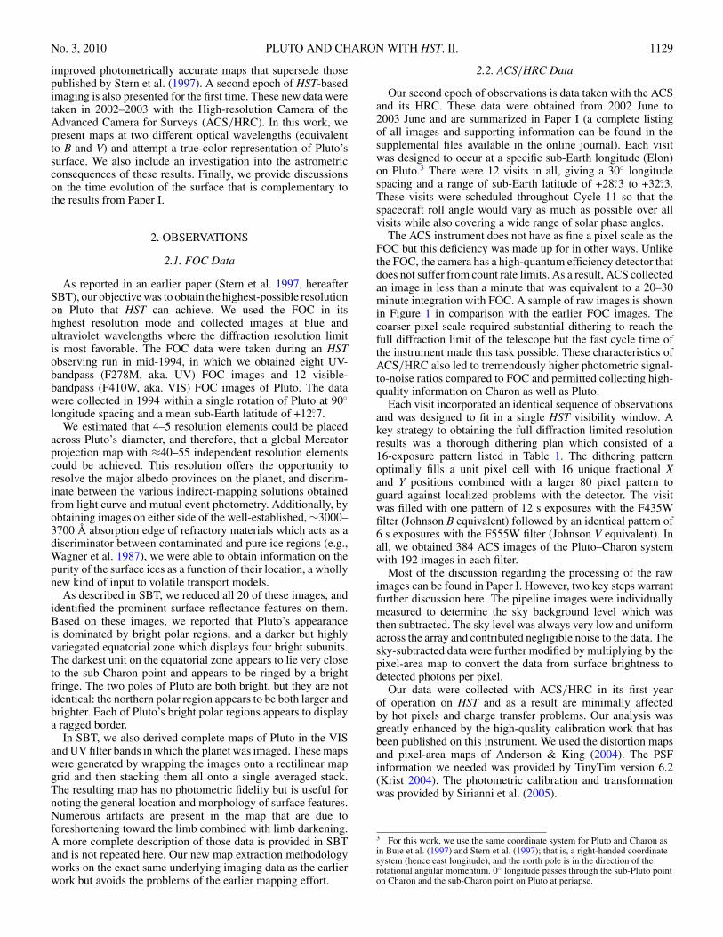
The ACS instrument does not have as fine a pixel scale as theFOC but this deficiency was made up for in other ways. Unlikethe FOC, the camera has a high-quantum efficiency detector thatdoes not suffer from count rate limits. As a result, ACS collectedan image in less than a minute that was equivalent to a 20–30minute integration with FOC. A sample of raw images is shownin Figure 1 in comparison with the earlier FOC images. Thecoarser pixel scale required substantial dithering to reach thefull diffraction limit of the telescope but the fast cycle time ofthe instrument made this task possible. These characteristics ofACS/HRC also led to tremendously higher photometric signal-to-noise ratios compared to FOC and permitted collecting high-quality information on Charon as well as Pluto.
Each visit incorporated an identical sequence of observationsand was designed to fit in a single HST visibility window. Akey strategy to obtaining the full diffraction limited resolutionresults was a thorough dithering plan which consisted of a16-exposure pattern listed in Table 1. The dithering patternoptimally fills a unit pixel cell with 16 unique fractional Xand Y positions combined with a larger 80 pixel pattern toguard against localized problems with the detector. The visitwas filled with one pattern of 12 s exposures with the F435Wfilter (Johnson B equivalent) followed by an identical pattern of6 s exposures with the F555W filter (Johnson V equivalent). Inall, we obtained 384 ACS images of the Pluto–Charon systemwith 192 images in each filter.
Most of the discussion regarding the processing of the rawimages can be found in Paper I. However, two key steps warrantfurther discussion here. The pipeline images were individuallymeasured to determine the sky background level which wasthen subtracted. The sky level was always very low and uniformacross the array and contributed negligible noise to the data. Thesky-subtracted data were further modified by multiplying by thepixel-area map to convert the data from surface brightness todetected photons per pixel.
Our data were collected with ACS/HRC in its first yearof operation on HST and as a result are minimally affectedby hot pixels and charge transfer problems. Our analysis wasgreatly enhanced by the high-quality calibration work that hasbeen published on this instrument. We used the distortion mapsand pixel-area maps of Anderson & King (2004). The PSFinformation we needed was provided by TinyTim version 6.2(Krist 2004). The photometric calibration and transformationwas provided by Sirianni et al. (2005).
3 For this work, we use the same coordinate system for Pluto and Charon asin Buie et al. (1997) and Stern et al. (1997); that is, a right-handed coordinatesystem (hence east longitude), and the north pole is in the direction of therotational angular momentum. 0◦ longitude passes through the sub-Pluto pointon Charon and the sub-Charon point on Pluto at periapse.
1130 BUIE ET AL. Vol. 139
289
203
112
15
275 244 212
180 154 125
94 65 29
1 334 303
Figure 1. Sample raw images of Pluto. The numbers beneath each image are the sub-Earth East longitude (degrees) for that view. The leftmost column of imagesis the sample of FOC data shown in Stern et al. (1997). The other columns show a sample from the newer ACS/HRC data without removing the optical distortionsinherent in the newer camera. The image scale is chosen such that Pluto is roughly the same size in all images. The coarser sampling is quite evident in the ACS dataset. The images have all been rotated to put Pluto’s spin-north pole at the top. Pluto appears elongated in the ACS images in pseudo-random orientations as a result ofthe optical distortions and the large variation of spacecraft roll angle through the data collection. The images are scaled by brightness, within each camera’s data set,so that the light curve information is preserved.
3. FORWARD MODELING
3.1. Fitting Concepts
Here we describe our approach to fitting all of the im-age data sets in a process we call forward modeling. Thismethod starts with the requirement that data values (in thiscase image pixels) are never modified or manipulated be-yond the needs of the calibration. As such, the images are atime-stamped grid providing a spatially resolved flux measure-ment collected over a field of view encompassing the Plutosystem.
Our task in fitting the data is then reduced to a description ofthe scene that we think we are viewing. In this case, we have twoobjects that can be well approximated as spheres illuminated bythe Sun that reflect light to our telescope and detector. Implicit inthis approach is that we describe the sphere as having an albedoor other surface reflectance property that is allowed to vary asa function of location on the sphere. In our case, a map of thesurface is actually a description of the single-scattering albedowhich varies over the surface.
From this map, we can compute an image of Pluto andCharon at an arbitrarily high spatial resolution on the plane-of-the-sky given the geometric aspects for each image. Wethen downsample this perfect image, conserving flux, to anideal image grid appropriate to the instrument, convolve witha PSF, and apply the geometric distortion factors (if needed).The resulting image is intended to reproduce what would be
observed by the instrument. This model image can then beiterated through its free parameters (i.e., map values) usingnonlinear least-squares minimization to find the map that bestfits the data. This process thus fits a single, static map to a givenset of image data simultaneously and can take full advantage ofany overlap and dithering between images to find an answer thatbest describes all images. In the interest of investigating timevariability of the surface we chose to treat the FOC and ACSdata sets as completely independent rather than solving for onemap for all data.
3.2. Model Parameters
Our forward model requires a priori knowledge of thegeometry of the problem. For the radii of the objects we adopteda value of 1151 km for Pluto to be consistent with Buie et al.(1992) and 606 km for Charon (Sicardy et al. 2006, based onan early pre-publication value). The viewing geometry, latitudeand longitude of the sub-solar and sub-Earth points, and positionangle of the rotation axis, were computed with the same Charonephemeris as used by Buie et al. (1992). While none of thesevalues are considered to be the best, the errors thus introducedare small compared to the intrinsic errors of the mappingprocess. This work was spread over such a long duration andthe size of the computation effort was so large that it precludeda last-minute update to these values. The last geometric variablewas the position of the objects in the image, which was fittedfor in each image.
No. 3, 2010 PLUTO AND CHARON WITH HST. II. 1131
Table 1Dither Pattern
Step POSTARGx (arcsec) y
1 0.000 0.0002 −0.363 −0.4213 −0.726 −0.8424 −1.089 −1.2635 0.200 0.1166 −0.163 −0.3057 −0.525 −0.7268 −0.888 −1.1479 0.085 0.316
10 −0.278 −0.10511 −0.641 −0.52612 −1.004 −0.94713 −0.116 0.20014 −0.479 −0.22015 −0.842 −0.64116 −1.205 −1.062
The model also clearly requires information about the PSF ofthe instrument. For the FOC data we used high-quality observedPSFs that matched the filters we used (the same PSFs as usedby SBT). For the ACS/HRC data we used TinyTim to computenumerical PSFs that are based on the mean color of the object.Thanks to the work of Brown & Trujillo (2004) we knew toalso fit for the telescope focus on each image. Based on thisprior work, we had hoped to fit a focus trend with HST orbitallongitude and thus reduce the number of free parameters in themodel. Unfortunately, the sampling pattern and the actual focustrends of our data precluded such a simple approach. As a result,we were forced to fit the focus independently on all images.
We used the Hapke scattering theory (Hapke 1993) to com-pute the reflected light from the surface of Pluto (and Charonfor the ACS data). Our approach in adapting the Hapke theoryto this analysis follows very closely to the Buie et al. (1992)mutual event mapping. However, Buie et al. (1992) used thesimplest form of the Hapke bidirectional reflectance equationfrom Hapke (1981), which makes no corrections for macro-scopic surface roughness. We have now added this term to ourcalculation as well as incorporating the newer definition for h,the surface compaction parameter (Hapke 1984). We found themacroscopic roughness term to be critical in providing com-putationally sensible center-to-limb profiles. Without this term,points on the extreme edge of the disk take on unphysically highI/F values, high enough to add a non-trivial contribution to theintegral over the disk in our calculations. Adding the roughnessterm, with almost any value for θ , eliminates this numericaldifficulty and the reflectance at the limb behaves sensibly.
In all, there are five free parameters that must be specifiedfor each map element so that a reflected flux can be computed.These parameters are w, single scattering albedo; h, surfacecompaction parameter; P (g), the single scattering particle phasefunction averaged over the small range of phase angle (g)we sample; B0, the backscatter correction factor; and θ , theaverage surface slope. It is a common practice to use a Henyey-Greenstein function (one or two parameters) for P (g) and thenfit for the coefficients of the function. However, our phase anglerange is so small and does a very poor job of constraining thisfunction. Our approach, consistent with our past publications,is to use a constant value for our data. This value, P (g), doesnot make any assumptions about the functional form but simplygives a constraint on any future choice of P (g).
Table 2Global Hapke Parameters
Set h P (g) B0 θ χ2VIS χ2
UV
A 0.1 2.5 0.8 10 1.26 0.76B 0.07 2.5 0.53 10 1.27 0.76C 0.05 2.5 0.39 10 1.28 0.76D 0.11 2.0 1.0 10 1.27 0.76E 0.122 3.0 1.0 10 1.25 0.78F 0.1 2.5 0.8 30 1.27 0.76Ch 0.0039 2.52 0.53 20 . . . . . .
We do not have sufficient data to determine all these quan-tities for each surface element. As is commonly done, we useglobal values for all of these parameters except for the sin-gle scattering albedo. The choice for the global scattering pa-rameters is not entirely arbitrary. As was done in Buie et al.(1992), we used the global photometric properties of Pluto toconstrain these values. When we started this project the datadid not yet yield a unique set of values, so we produced anumber of plausible sets of parameters that spanned the plau-sible range of values expected on the surfaces of Pluto andCharon.
To constrain the global values, we used a sphere with auniform single-scattering albedo of w = 0.8. We then computethe disk-integrated magnitude over the same range of solar phaseangles possible for Pluto (and Charon) in 1992. By picking avalue of h, we searched for the values of P (g) and B0 that wouldmatch a phase coefficient of β = 0.0294 mag deg−1 for Plutoand β = 0.0866 mag deg−1 for Charon from Buie et al. (1997).We found the phase behavior to be completely insensitive tosurface roughness, not surprising since surface roughness doesnot become truly important until the phase angle reaches 30◦–40◦ (Hapke 1984). Therefore, we chose values for θ that seemedconsistent with other similar surfaces in the solar system. Thevalue chosen for θ for Pluto was based on Triton, though wetried one test using a larger value (set F). The Charon valueswere chosen to be consistent with other water–ice surfaces. Theresults of this calculation are summarized in Table 2. Sets A–Fdescribe global values that all mimic the phase behavior of Pluto.The last set (Ch) is consistent with the phase behavior of Charon(see Paper I). Given the input constraints, none of these valueswere unique and a suite of parameters was chosen for Plutoto facilitate some consistency checks in fitting the FOC data.However, note that all of these parameter sets include a largevalue for P (g), indicating the particles have a backscatteringlobe in their single-particle phase function.
Our fitting process works in absolute flux units (erg cm−2 s−1).The images are converted from instrumental counts to flux byusing the PHOTFLAM header value. The conversion from bidi-rectional reflectance to absolute flux uses the known geocentricand heliocentric distance of Pluto (Δ and r, respectively) as wellas the absolute flux of the Sun integrated over the instrumentalbandpass. The steps required to go from the list of free param-eters to something that is compared directly to the data are asfollows:
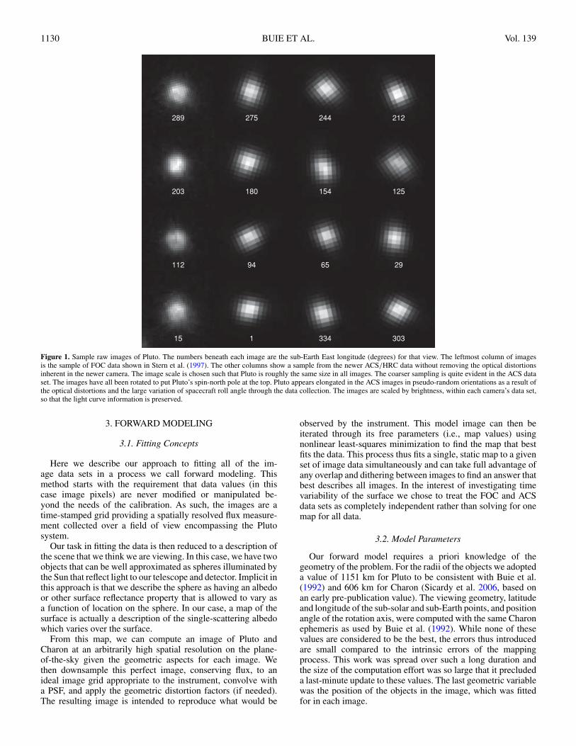
1. The list of map value free and fixed parameters is convertedfrom its lookup table to a small (18 × 10 for ACS data,20 × 10 for FOC data) regular grid. This grid of single-scattering albedo is expanded by pixel replication to a360×200 grid. The fitting grids with the converged valuesof w are shown in Figure 2 for Pluto and in Figure 3 forCharon. This expanded grid is then smoothed by a spherical
1132 BUIE ET AL. Vol. 139
Gaussian filter with an FWHM of 15◦ (30◦ for Charon)on the surface of the sphere. The choice of sub-samplingfactors was made by requiring the photometric error fromthe rendered images as a function of sub-Earth longitude tobe no worse than 0.1%. The width of the Gaussian filter waschosen to impose a limit on the spatial frequencies in theoutput image comparable to the diffraction limit of HST.The unconstrained polar regions were combined with cellsthat are visible near the winter terminator. By replicatingthe regions from the terminator to the invisible pole thecalculation becomes numerically well behaved. The totalnumber of free parameters in the FOC map grid was 144,while the ACS/HRC map has 114. The Charon ACS/HRCmap grid has 25 free parameters.
2. A bidirectional reflectance image was computed from thesmoothed map for the appropriate sub-Earth and sub-solarlatitude and longitude at a scale that is a factor of 23smaller than the undistorted pixel scale for HRC and afactor of 10 for FOC. The choice of the pixel scale was acompromise between speed of execution (lower is faster)and numerically well behaved (larger is better). This scaleincludes a conversion from the spatial scale in kilometersbased on the radius of Pluto (or Charon) to arcsecondsand all the geometric information (e.g., r,Δ) unique to eachexposure. The sub-sampling factor was chosen to keep thephotometric errors of the finite rendered grid at or below0.1%. This test was done by computing the numericalintegral over the disk on the rendered image as a functionof the position in the image plane. Numerical integrationnoise is seen as the position is moved across the scaleof a single pixel and this quantity is minimized by thechosen sampling scale. The position at which this imageis located introduces two free parameters in the renderedimage calculation. The known orientation of the image, asdescribed by the ORIENTAT keyword, was applied so thatthe position angle of Pluto’s rotation axis in the renderedimage matches that angle on the undistorted sky plane asseen in each image.
3. The sub-sampled sky-plane image is then binned down bypixel summation to match the instrumental pixel griddingscale. Finally, the computed image is then combined withthe appropriate PSF including distortion if needed. At theend of this step, we have an image that can be directlycompared to the data.
Our fitting process used the above steps to compute a weightedgoodness-of-fit statistic for the given set of data and a uniqueset of free parameters. Not all free parameters are solved for atthe same time. The fitting is broken into three discrete steps: (1)fit the map, (2) fit the positions, and (3) fit the focus (ACS dataonly). For each of the steps, the other free parameters are heldconstant. The order in which the steps are performed does notaffect the final answer but the convergence time was reducedby alternately fitting the map, fitting the positions, re-fitting themap, fitting focus, re-fitting the map again, and so on until nochanges were seen at any step.
3.3. FOC Model
The reference solar flux at 1 AU used by the FOC model was184 erg cm−2 s−1 for the F410W filter and 22.6 erg cm−2 s−1
for the F278M filter and was derived by integrating overthe instrumental response from the solar atlas of A’Hearnet al. (1983). Map fits were completed for all six sets of
-90
-45
0
45
90
Latitu
de (
degre
es)
AC
S/H
RC
- F
555W
2002/2
003
-90
-45
0
45
90
Latitu
de (
degre
es)
AC
S/H
RC
- F
435W
2002/2
003
-90
-45
0
45
90
Latitu
de (
degre
es)
FO
C/H
RC
- F
410M
1994
270 0 90 180 270East Longitude (degrees)
-90
-45
0
45
90
Latitu
de (
degre
es)
AC
S r
esolu
tion
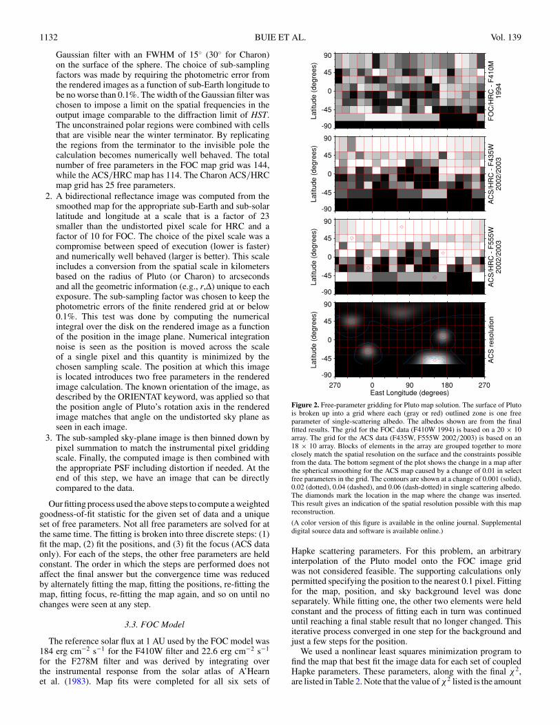
Figure 2. Free-parameter gridding for Pluto map solution. The surface of Plutois broken up into a grid where each (gray or red) outlined zone is one freeparameter of single-scattering albedo. The albedos shown are from the finalfitted results. The grid for the FOC data (F410W 1994) is based on a 20 × 10array. The grid for the ACS data (F435W, F555W 2002/2003) is based on an18 × 10 array. Blocks of elements in the array are grouped together to moreclosely match the spatial resolution on the surface and the constraints possiblefrom the data. The bottom segment of the plot shows the change in a map afterthe spherical smoothing for the ACS map caused by a change of 0.01 in selectfree parameters in the grid. The contours are shown at a change of 0.001 (solid),0.02 (dotted), 0.04 (dashed), and 0.06 (dash-dotted) in single scattering albedo.The diamonds mark the location in the map where the change was inserted.This result gives an indication of the spatial resolution possible with this mapreconstruction.
(A color version of this figure is available in the online journal. Supplementaldigital source data and software is available online.)
Hapke scattering parameters. For this problem, an arbitraryinterpolation of the Pluto model onto the FOC image gridwas not considered feasible. The supporting calculations onlypermitted specifying the position to the nearest 0.1 pixel. Fittingfor the map, position, and sky background level was doneseparately. While fitting one, the other two elements were heldconstant and the process of fitting each in turn was continueduntil reaching a final stable result that no longer changed. Thisiterative process converged in one step for the background andjust a few steps for the position.
We used a nonlinear least squares minimization program tofind the map that best fit the image data for each set of coupledHapke parameters. These parameters, along with the final χ2,are listed in Table 2. Note that the value of χ2 listed is the amount

No. 3, 2010 PLUTO AND CHARON WITH HST. II. 1133
-90
-45
0
45
90
Latitu
de (
degre
es)
AC
S/H
RC
- F
555W
2002/2
003
-90
-45
0
45
90Latitu
de (
degre
es)
AC
S/H
RC
- F
435W
2002/2
003
270 0 90 180 270East Longitude (degrees)
-90
-45
0
45
90
Latitu
de (
degre
es)
AC
S r
esolu
tion
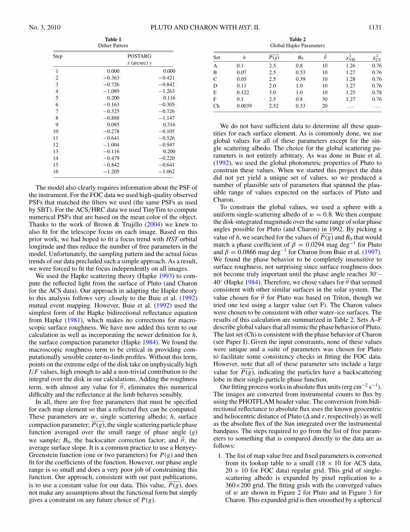
Figure 3. Free-parameter gridding for Charon map solution. The surface ofCharon is broken up into a grid where each outlined zone is one free parameterof single-scattering albedo and is based on an underlying 18 × 10 array. Thealbedos shown are from the final fitted results. Blocks of elements in the arrayare grouped together to more closely match the spatial resolution on the surfaceand the constraints possible from the data. The bottom segment of the plot showsa point response of the map calculation. The contours are shown at a changeof 0.001 (solid), 0.02 (dotted), 0.04 (dashed), and 0.06 (dash-dotted) in singlescattering albedo after the spherical smoothing from an initial change of 0.1 inthe map grid. The diamonds mark the location in the map where the change wasinserted. This result gives an indication of the spatial resolution possible withthis map reconstruction.
(A color version of this figure is available in the online journal. Supplementaldigital source data and software is available online.)
per degree of freedom. We also weighted each image data valueby its expected uncertainty assuming photon counting statistics.Since the FOC is a photon counting instrument, this assumptionshould be very good. Each of these sets (A–F) of Hapkeparameters worked equally well in deriving a map accordingto the final goodness-of-fit statistic. We have arbitrarily chosenset A as our adopted set of parameters. This choice was guidedby picking a set that falls in the middle of the range of validparameters. The visual appearance of the fitted maps is thesame, further demonstrating that the fitting process reaches thesame result for a different set of fitting parameters.
3.4. ACS/HRC Model
The reference solar flux at 1 AU for the ACS modelwas 170.384 erg cm−2 s−1 for the F435W filter and187.463 erg cm−2 s−1 for the F555W filter and was derivedby integrating over the instrumental response from the solarspectrum of Colina et al. (1996). It was not practical to fit all sixsets of Hapke parameters so we fitted these data using only setA. Unlike the FOC map, the ACS model did not discretize thesky-plane position.
The PSF used was generated by TinyTim version 6.2 (Krist2004) using our independently fitted focus position (z4 Zernike
term) for each image. This numerical PSF was calculated at afactor of 3 finer interval than the idealized pixel scale so thatthe PSF was interpolatable. At the very end of the calculation,the numerical PSF and the model image were passed to thefinal stage (tiny3) of the TinyTim package that then appliesthe geometric distortion across the entire image. It is this stepthat consumed virtually all of the CPU time for the fittingprocess.
The focus fitting process used discretized focus values thatscanned over the range of −1 � z4 � 1 at a step size of 0.001to find the overall lowest χ2 for each image. A small fractionof the images did not yield appropriate fitted values for focus.These special cases were assigned a non-fitted focus value thatwas determined by visual inspection and evaluation of the focustrends from adjacent images where the focus fit worked moreconvincingly.
The complete fitting process involved iterating betweenadjusting the map, position, and telescope focus. The positionsand focus were fit just a few times during the entire process.The bulk of the fitting work was iterating on the map. Givena map, the fit for focus and position was relatively quick (lessthan an hour of CPU time). The map fitting step was very slowgiven the computational cost of the image distortion calculation.Convergence from a given starting point took roughly 16 weekson a 20-node parallel computing cluster. A limited number ofstarting values were processed to help constrain the uncertaintyon the final map product. These starting values were a uniformmap with w = 0.8 and a map derived from the FOC results.There were three sets of data fitted: (1) the first six visits in timeorder, (2) the last six visits, and (3) all the visits together. Thevisits were scheduled such that the first six were scheduled at theend of the 2002 apparition of Pluto with a 60◦ longitude spacing.The other six visits were in the first half of the 2003 apparitionwith a 60◦ longitude spacing but shifted by 30◦ from the otherset of visits. As the fitting progressed, other intermediate mapswere generated by using a converged map from a different dataset or starting point. In all, we generated partially convergedmaps for 11 cases for the B (F435W) map and five cases for theV (F555W) map. Despite the many cases tried, only one solutioncould be brought to a final converged solution due to changesin calibrations and fitting technique that crept in during the longfitting process. We present here the results from fitting all thedata in each filter that started from a uniform albedo map. Theother partially converged results are used only to confirm thestability of the fitting process.
The fitting process did a very good job of matching the modelimage to the data. Some examples of the data and the imageresiduals are shown in Figure 4. Two representative images andtheir residuals are shown for each visit and each filter. The choiceof pattern step number was made to highlight differences (or lackthereof) caused by dithering. The residuals are not completelyrandom and point to systematic problems unique to each visit.Jitter has been ruled out as a contributing factor but many otherpossibilities remain, such as charge diffusion in the CCD andimperfections in the size of the core of the PSF.
4. MAPS
4.1. Pluto
Figure 5 shows the final maps of Pluto’s surface fromour new analysis. For comparison, the map from Buie et al.(1992) is shown at the same scale (top panel). To allow thevisual comparison of the maps, each has been converted to
1134 BUIE ET AL. Vol. 139
11
data resid data resid
66
data resid data resid
F555W F435W
1
2
3
4
5
6
7
8
9
10
11
12
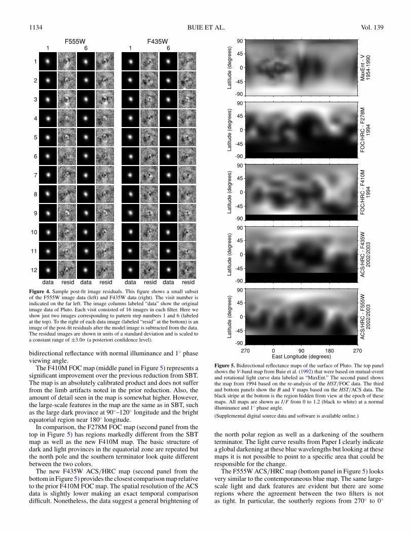
Figure 4. Sample post-fit image residuals. This figure shows a small subsetof the F555W image data (left) and F435W data (right). The visit number isindicated on the far left. The image columns labeled “data” show the originalimage data of Pluto. Each visit consisted of 16 images in each filter. Here weshow just two images corresponding to pattern step numbers 1 and 6 (labeledat the top). To the right of each data image (labeled “resid” at the bottom) is animage of the post-fit residuals after the model image is subtracted from the data.The residual images are shown in units of a standard deviation and is scaled toa constant range of ±3.0σ (a posteriori confidence level).
bidirectional reflectance with normal illuminance and 1◦ phaseviewing angle.
The F410M FOC map (middle panel in Figure 5) represents asignificant improvement over the previous reduction from SBT.The map is an absolutely calibrated product and does not sufferfrom the limb artifacts noted in the prior reduction. Also, theamount of detail seen in the map is somewhat higher. However,the large-scale features in the map are the same as in SBT, suchas the large dark province at 90◦–120◦ longitude and the brightequatorial region near 180◦ longitude.
In comparison, the F278M FOC map (second panel from thetop in Figure 5) has regions markedly different from the SBTmap as well as the new F410M map. The basic structure ofdark and light provinces in the equatorial zone are repeated butthe north pole and the southern terminator look quite differentbetween the two colors.
The new F435W ACS/HRC map (second panel from thebottom in Figure 5) provides the closest comparison map relativeto the prior F410M FOC map. The spatial resolution of the ACSdata is slightly lower making an exact temporal comparisondifficult. Nonetheless, the data suggest a general brightening of
270 0 90 180 270East Longitude (degrees)
-90
-45
0
45
90
Latitu
de (
degre
es)
AC
S/H
RC
- F
55
5W
2002/2
003
-90
-45
0
45
90Latitu
de (
degre
es)
AC
S/H
RC
- F
43
5W
2002/2
003
-90
-45
0
45
90
Latitu
de (
degre
es)
FO
C/H
RC
- F
410M
1994
-90
-45
0
45
90
Latitu
de (
degre
es)
FO
C/H
RC
- F
27
8M
1994
-90
-45
0
45
90
Latitu
de (
degre
es)
MaxE
nt -
V1954-1
990
Figure 5. Bidirectional reflectance maps of the surface of Pluto. The top panelshows the V-band map from Buie et al. (1992) that were based on mutual-eventand rotational light curve data labeled as “MaxEnt.” The second panel showsthe map from 1994 based on the re-analysis of the HST/FOC data. The thirdand bottom panels show the B and V maps based on the HST/ACS data. Theblack stripe at the bottom is the region hidden from view at the epoch of thesemaps. All maps are shown as I/F from 0 to 1.2 (black to white) at a normalilluminance and 1◦ phase angle.
(Supplemental digital source data and software is available online.)
the north polar region as well as a darkening of the southernterminator. The light curve results from Paper I clearly indicatea global darkening at these blue wavelengths but looking at thesemaps it is not possible to point to a specific area that could beresponsible for the change.
The F555W ACS/HRC map (bottom panel in Figure 5) looksvery similar to the contemporaneous blue map. The same large-scale light and dark features are evident but there are someregions where the agreement between the two filters is notas tight. In particular, the southerly regions from 270◦ to 0◦
No. 3, 2010 PLUTO AND CHARON WITH HST. II. 1135
270°
180°
90°
0°
Lat=0°1954-1990
MaxEntB and V
Lat=12°1994
FOC/HRCF410M
Lat=30°2002-2003
ACS/HRCF435W
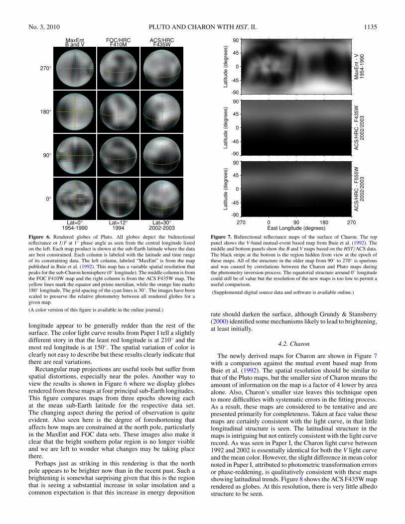
Figure 6. Rendered globes of Pluto. All globes depict the bidirectionalreflectance or I/F at 1◦ phase angle as seen from the central longitude listedon the left. Each map product is shown at the sub-Earth latitude where the dataare best constrained. Each column is labeled with the latitude and time rangeof its constraining data. The left column, labeled “MaxEnt” is from the mappublished in Buie et al. (1992). This map has a variable spatial resolution thatpeaks for the sub-Charon hemisphere (0◦ longitude). The middle column is fromthe FOC F410W map and the right column is from the ACS F435W map. Theyellow lines mark the equator and prime meridian, while the orange line marks180◦ longitude. The grid spacing of the cyan lines is 30◦. The images have beenscaled to preserve the relative photometry between all rendered globes for agiven map.
(A color version of this figure is available in the online journal.)
longitude appear to be generally redder than the rest of thesurface. The color light curve results from Paper I tell a slightlydifferent story in that the least red longitude is at 210◦ and themost red longitude is at 150◦. The spatial variation of color isclearly not easy to describe but these results clearly indicate thatthere are real variations.
Rectangular map projections are useful tools but suffer fromspatial distortions, especially near the poles. Another way toview the results is shown in Figure 6 where we display globesrendered from these maps at four principal sub-Earth longitudes.This figure compares maps from three epochs showing eachat the mean sub-Earth latitude for the respective data set.The changing aspect during the period of observation is quiteevident. Also seen here is the degree of foreshortening thataffects how maps are constrained at the north pole, particularlyin the MaxEnt and FOC data sets. These images also make itclear that the bright southern polar region is no longer visibleand we are left to wonder what changes may be taking placethere.
Perhaps just as striking in this rendering is that the northpole appears to be brighter now than in the recent past. Such abrightening is somewhat surprising given that this is the regionthat is seeing a substantial increase in solar insolation and acommon expectation is that this increase in energy deposition
270 0 90 180 270East Longitude (degrees)
-90
-45
0
45
90
Latitu
de (
degre
es)
AC
S/H
RC
- F
55
5W
2002/2
003
-90
-45
0
45
90
Latitu
de (
degre
es)
AC
S/H
RC
- F
435W
2002/2
003
-90
-45
0
45
90
Latitu
de (
degre
es)
MaxE
nt -
V1954-1
990
Figure 7. Bidirectional reflectance maps of the surface of Charon. The toppanel shows the V-band mutual-event based map from Buie et al. (1992). Themiddle and bottom panels show the B and V maps based on the HST/ACS data.The black stripe at the bottom is the region hidden from view at the epoch ofthese maps. All of the structure in the older map from 90◦ to 270◦ is spuriousand was caused by correlations between the Charon and Pluto maps duringthe photometry inversion process. The equatorial structure around 0◦ longitudecould still be of value but the resolution of the new maps is too low to permit auseful comparison.
(Supplemental digital source data and software is available online.)
rate should darken the surface, although Grundy & Stansberry(2000) identified some mechanisms likely to lead to brightening,at least initially.
4.2. Charon
The newly derived maps for Charon are shown in Figure 7with a comparison against the mutual event based map fromBuie et al. (1992). The spatial resolution should be similar tothat of the Pluto maps, but the smaller size of Charon means theamount of information on the map is a factor of 4 lower by areaalone. Also, Charon’s smaller size leaves this technique opento more difficulties with systematic errors in the fitting process.As a result, these maps are considered to be tentative and arepresented primarily for completeness. Taken at face value thesemaps are certainly consistent with the light curve, in that littlelongitudinal structure is seen. The latitudinal structure in themaps is intriguing but not entirely consistent with the light curverecord. As was seen in Paper I, the Charon light curve between1992 and 2002 is essentially identical for both the V light curveand the mean color. However, the slight difference in mean colornoted in Paper I, attributed to photometric transformation errorsor phase-reddening, is qualitatively consistent with these mapsshowing latitudinal trends. Figure 8 shows the ACS F435W maprendered as globes. At this resolution, there is very little albedostructure to be seen.

1136 BUIE ET AL. Vol. 139
270 240 210
180 150 120
90 60 30
0 330 300
Figure 8. Rendered globes of Charon. All globes depict the bidirectionalreflectance or I/F at 1◦ phase angle from the ACS F435W map at the meanlatitude (30◦) in 2002/2003. The central longitude of each globe is given to thelower left. The yellow lines mark the equator and prime meridian, while theorange line marks 180◦ longitude. The grid spacing of the cyan lines is 30◦.The images have been scaled to preserve the relative photometry between allrendered globes. The sequence of globes lets you see the satellite as it rotates(longitude decreasing with time).
(A color version of this figure is available in the online journal.)
The MaxEnt maps for Charon have long been a puzzle. Buieet al. (1997) pointed out that the map could not be correct since itpredicts the wrong light curve. However, this categorical denialof the entire map may have been premature. Certainly the portionof the map from 90◦ to 270◦ is not useful in the MaxEnt mapbecause that area was constrained by combined light photometry(Pluto+Charon). However, the sub-Pluto hemisphere, centeredat 0◦, is directly constrained by mutual event light curve dataand as such should contain some measure of truth. The MaxEntmap does contain an element of latitudinal variation similar tothat seen in the ACS maps suggesting that the latitudinal trendcould be real.
5. DERIVED MAP PRODUCTS
The maps presented in the previous section are the directresult of the fitting process and represent the primary result ofthis work. There are other secondary results that come fromfurther analysis of the maps or the statistical output of the fittingprocess.
5.1. Albedo Change with Time
The light curve results in Paper I already indicate a significantchange at a global level for Pluto’s albedo versus time. Weexamined the fitting results in search of a signature that couldbe related to this change. Figures 9 and 10 attempt to showthe goodness-of-fit on an image combined with a sensitivity
matrix that shows how each image constrains (or not) eachfree parameter. The details of the constructed image are in thecaption, but these complicated data products are better viewedfrom a larger perspective. In this rendering, mid-level graycorresponds to either a perfect fit of the model to the data orno constraint at all. The diagonal gray stripes basically showwhere given tiles in the map are not visible as Pluto rotates. Theareas in between show the constrained regions. If a model imageis too dark relative to the data then that pixel will be darker thana perfect fit. If the model image is too bright then you see abrighter region.
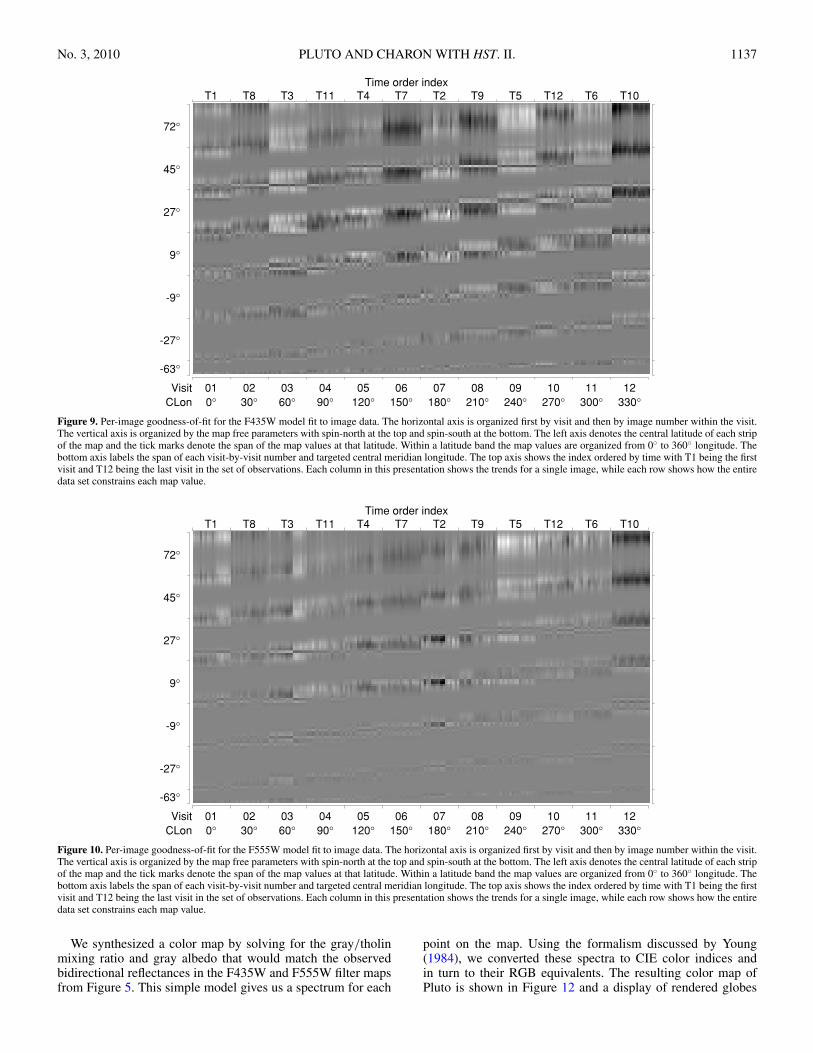
Looking at the information for the F435W data in Figure 9,one sees a striking light/dark pattern between odd and even visitnumbers. Recall that the odd visit numbers were taken as a set inthe first half of Cycle 11 and that the even visit numbers were inthe latter half of the cycle. In this view, it is easy to see that themodel trends from being too dark early in the cycle to being toobright late in the cycle, relative to the data. There is clearly somelongitudinal structure to the temporal variation since the patternis not perfect. When compared to the F555W result in Figure 10,there are some visits with systematic errors (especially visit 9)but the overall temporal pattern seen with F435W is absent. Keepin mind that the forward model includes all purely geometricchanges that occur during the observations. Since the modelincludes geometric change but not temporal change, the lack oftemporally structured residuals in the F555W data is consistentwith a static map during Cycle 11. The temporally structuredresiduals in the map fits to the F435W data clearly point toa failure of the model to track the data as it did for F555W.The most likely interpretation of these residual patterns is theexistence of unmodeled temporal variations in albedo during theyear.
5.2. UV Color Map
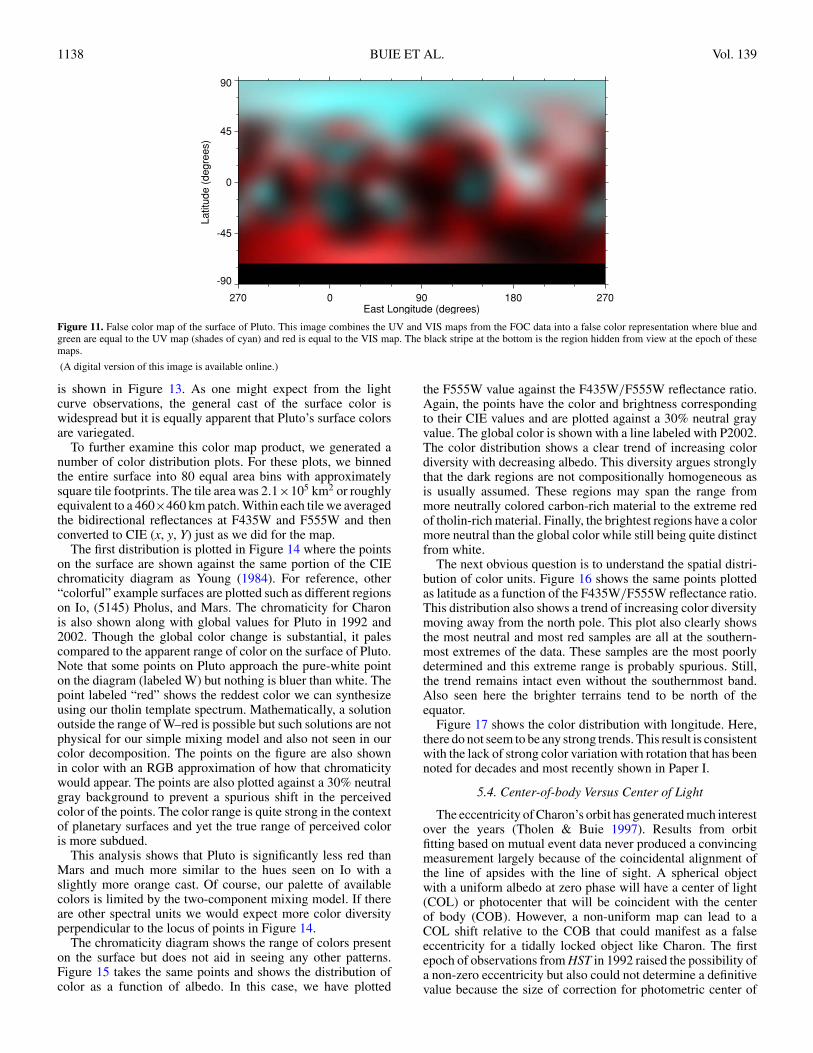
The FOC maps were intended to test for ice purity byobtaining data in the ultraviolet. Figure 11 shows a false-colorrendering of the FOC maps. In this figure, neutral reflectancewould be white (or gray). Blue regions indicate where the I/Fis higher in the UV than in the visible. Red regions indicate UVdark areas. The north polar regions and the bright equatorialspot at 180◦ longitude are UV bright, consistent with clean ice.Possible explanations for a region being UV dark include theaccumulation of photolytic or radiolytic residues in the polarice or removal of ice exposing these materials in an ancientsubstrate.
5.3. Optical Color Map
One of the goals of this program was to attempt color mapsof the surface of Pluto. With only two wavelengths sampled, itis not possible to directly create a true color image. However,the spectrum of Pluto at visible wavelengths is known to befree of any strong absorption features making it feasible tosynthesize a plausible facsimile. Given that the continuumabsorbing reddening agent is expected to be related to high-order hydrocarbons, we created a simple spectral mixing modelusing a gray reflector with an extreme-red laboratory tholinspectrum. The tholin spectrum choice was dictated by needingsomething as red as the reddest point in the Pluto maps. Thebase spectrum we used was the Triton tholin of Khare et al.(1994) computed for a 4 μm grain size. We do not attach anyparticular significance to the details of the synthetic spectrumexcept that it represents something close to an actual spectrumfor a plausible surface component.
No. 3, 2010 PLUTO AND CHARON WITH HST. II. 1137
T1
01
0°
T8
02
30°
T3
03
60°
T11
04
90°
T4
05
120°
T7
06
150°
T2
07
180°
T9
08
210°
T5
09
240°
T12
10
270°
T6
11
300°
T10
12
330°
Time order index
Visit
CLon
72°
45°
27°
9°
-9°
-27°
-63°
Figure 9. Per-image goodness-of-fit for the F435W model fit to image data. The horizontal axis is organized first by visit and then by image number within the visit.The vertical axis is organized by the map free parameters with spin-north at the top and spin-south at the bottom. The left axis denotes the central latitude of each stripof the map and the tick marks denote the span of the map values at that latitude. Within a latitude band the map values are organized from 0◦ to 360◦ longitude. Thebottom axis labels the span of each visit-by-visit number and targeted central meridian longitude. The top axis shows the index ordered by time with T1 being the firstvisit and T12 being the last visit in the set of observations. Each column in this presentation shows the trends for a single image, while each row shows how the entiredata set constrains each map value.
T1
01
0°
T8
02
30°
T3
03
60°
T11
04
90°
T4
05
120°
T7
06
150°
T2
07
180°
T9
08
210°
T5
09
240°
T12
10
270°
T6
11
300°
T10
12
330°
Time order index
Visit
CLon
72°
45°
27°
9°
-9°
-27°
-63°
Figure 10. Per-image goodness-of-fit for the F555W model fit to image data. The horizontal axis is organized first by visit and then by image number within the visit.The vertical axis is organized by the map free parameters with spin-north at the top and spin-south at the bottom. The left axis denotes the central latitude of each stripof the map and the tick marks denote the span of the map values at that latitude. Within a latitude band the map values are organized from 0◦ to 360◦ longitude. Thebottom axis labels the span of each visit-by-visit number and targeted central meridian longitude. The top axis shows the index ordered by time with T1 being the firstvisit and T12 being the last visit in the set of observations. Each column in this presentation shows the trends for a single image, while each row shows how the entiredata set constrains each map value.
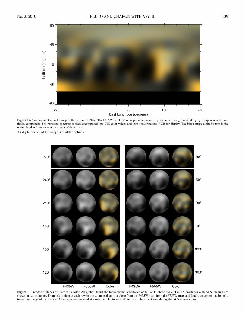
We synthesized a color map by solving for the gray/tholinmixing ratio and gray albedo that would match the observedbidirectional reflectances in the F435W and F555W filter mapsfrom Figure 5. This simple model gives us a spectrum for each
point on the map. Using the formalism discussed by Young(1984), we converted these spectra to CIE color indices andin turn to their RGB equivalents. The resulting color map ofPluto is shown in Figure 12 and a display of rendered globes
1138 BUIE ET AL. Vol. 139
270 0 90 180 270East Longitude (degrees)
-90
-45
0
45
90
Latitu
de (
degre
es)
Figure 11. False color map of the surface of Pluto. This image combines the UV and VIS maps from the FOC data into a false color representation where blue andgreen are equal to the UV map (shades of cyan) and red is equal to the VIS map. The black stripe at the bottom is the region hidden from view at the epoch of thesemaps.
(A digital version of this image is available online.)
is shown in Figure 13. As one might expect from the lightcurve observations, the general cast of the surface color iswidespread but it is equally apparent that Pluto’s surface colorsare variegated.
To further examine this color map product, we generated anumber of color distribution plots. For these plots, we binnedthe entire surface into 80 equal area bins with approximatelysquare tile footprints. The tile area was 2.1×10⁵ km2 or roughlyequivalent to a 460×460 km patch. Within each tile we averagedthe bidirectional reflectances at F435W and F555W and thenconverted to CIE (x, y, Y) just as we did for the map.
The first distribution is plotted in Figure 14 where the pointson the surface are shown against the same portion of the CIEchromaticity diagram as Young (1984). For reference, other“colorful” example surfaces are plotted such as different regionson Io, (5145) Pholus, and Mars. The chromaticity for Charonis also shown along with global values for Pluto in 1992 and2002. Though the global color change is substantial, it palescompared to the apparent range of color on the surface of Pluto.Note that some points on Pluto approach the pure-white pointon the diagram (labeled W) but nothing is bluer than white. Thepoint labeled “red” shows the reddest color we can synthesizeusing our tholin template spectrum. Mathematically, a solutionoutside the range of W–red is possible but such solutions are notphysical for our simple mixing model and also not seen in ourcolor decomposition. The points on the figure are also shownin color with an RGB approximation of how that chromaticitywould appear. The points are also plotted against a 30% neutralgray background to prevent a spurious shift in the perceivedcolor of the points. The color range is quite strong in the contextof planetary surfaces and yet the true range of perceived coloris more subdued.
This analysis shows that Pluto is significantly less red thanMars and much more similar to the hues seen on Io with aslightly more orange cast. Of course, our palette of availablecolors is limited by the two-component mixing model. If thereare other spectral units we would expect more color diversityperpendicular to the locus of points in Figure 14.
The chromaticity diagram shows the range of colors presenton the surface but does not aid in seeing any other patterns.Figure 15 takes the same points and shows the distribution ofcolor as a function of albedo. In this case, we have plotted
the F555W value against the F435W/F555W reflectance ratio.Again, the points have the color and brightness correspondingto their CIE values and are plotted against a 30% neutral grayvalue. The global color is shown with a line labeled with P2002.The color distribution shows a clear trend of increasing colordiversity with decreasing albedo. This diversity argues stronglythat the dark regions are not compositionally homogeneous asis usually assumed. These regions may span the range frommore neutrally colored carbon-rich material to the extreme redof tholin-rich material. Finally, the brightest regions have a colormore neutral than the global color while still being quite distinctfrom white.
The next obvious question is to understand the spatial distri-bution of color units. Figure 16 shows the same points plottedas latitude as a function of the F435W/F555W reflectance ratio.This distribution also shows a trend of increasing color diversitymoving away from the north pole. This plot also clearly showsthe most neutral and most red samples are all at the southern-most extremes of the data. These samples are the most poorlydetermined and this extreme range is probably spurious. Still,the trend remains intact even without the southernmost band.Also seen here the brighter terrains tend to be north of theequator.
Figure 17 shows the color distribution with longitude. Here,there do not seem to be any strong trends. This result is consistentwith the lack of strong color variation with rotation that has beennoted for decades and most recently shown in Paper I.
5.4. Center-of-body Versus Center of Light
The eccentricity of Charon’s orbit has generated much interestover the years (Tholen & Buie 1997). Results from orbitfitting based on mutual event data never produced a convincingmeasurement largely because of the coincidental alignment ofthe line of apsides with the line of sight. A spherical objectwith a uniform albedo at zero phase will have a center of light(COL) or photocenter that will be coincident with the centerof body (COB). However, a non-uniform map can lead to aCOL shift relative to the COB that could manifest as a falseeccentricity for a tidally locked object like Charon. The firstepoch of observations from HST in 1992 raised the possibility ofa non-zero eccentricity but also could not determine a definitivevalue because the size of correction for photometric center of
No. 3, 2010 PLUTO AND CHARON WITH HST. II. 1139
270 0 90 180 270
East Longitude (degrees)
-90
-45
0
45
90
Latitu
de (
degre
es)
Figure 12. Synthesized true-color map of the surface of Pluto. The F435W and F555W maps constrain a two-parameter mixing model of a gray component and a redtholin component. The resulting spectrum is then decomposed into CIE color values and then converted into RGB for display. The black stripe at the bottom is theregion hidden from view at the epoch of these maps.
(A digital version of this image is available online.)
270°
240°
210°
180°
150°
120°
90°
60°
30°
0°
330°
300°
F435W F555W Color F435W F555W Color
Figure 13. Rendered globes of Pluto with color. All globes depict the bidirectional reflectance or I/F at 1◦ phase angle. The 12 longitudes with ACS imaging areshown in two columns. From left to right at each row in the columns there is a globe from the F435W map, from the F555W map, and finally an approximation of atrue-color image of the surface. All images are rendered at a sub-Earth latitude of 31◦ to match the aspect seen during the ACS observations.

1140 BUIE ET AL. Vol. 139
0.32 0.34 0.36 0.38 0.40 0.42CIE x
0.32
0.34
0.36
0.38
0.40
CIE
y
0.32 0.34 0.36 0.38 0.40 0.42CIE x
0.32
0.34
0.36
0.38
0.40
CIE
y
Io 1
Io 3f
Io 3a
red
P2002
P1992
Pholus
Charon
Mars
Io 060
Io 263
W
87moderate
yellow
73pale
orangeyellow
71moderateorangeyellow
52light
orange
29 modera
te
yello
wish p
ink
90grayishyellow
105grayish
greenishyellow
102moderategreenishyellow
119 li
ght
yello
w g
reen
121pale
yellowgreen
93 y
ello
wis
h gr
ey
33 bronwish pink
Figure 14. Distribution of terrain color on Pluto. This plot shows the portionof the CIE chromaticity diagram that is relevant to the range of surface coloron Pluto plus some of the more colorful solid surfaces in the solar system. Thebackground in the plot is set to a 30% gray value to facilitate the perception ofthe displayed colors. The faint black lines on the background show the colorboundaries from the translation of standard Munsell color domains. The pointslabeled as Io show different regions (1, 3a, and 3f as described by Young 1984)and different global colors (leading hemisphere, 60◦ and trailing hemisphere,263◦ longitude from the spectra of Spencer et al. 1995). Also included is acolor for Mars using the average spectrum for the bright terrains from Mustard& Bell (1994). The dots along the diagonal show the colors for various areason the surface of Pluto. Also shown are two reference “colors” for white (W –Illuminant C) and “red” (see the text for details). All symbols are plotted withthe color of the point on the chromaticity diagram using the highest illuminancevalue (Y) that does not saturate any of the RGB values. A constant value of Y =0.53 is used for all Pluto terrains to prevent color saturation. The point labeled“P2002” is the global averaged color for Pluto in 2002 and “P1992” shows theglobally averaged color in 1992. All values with x>0.34 correspond to a NBScolor value of 90 “grayish yellow.” Lower values of x lie in region 93 “yellowishgray.” The area represented by each point is 2.1×10⁵ km2 (1/80 of total surfacearea).
(An enhanced color version of this figure is available in the online journal.)
P2002W red
1.0 0.8 0.6 0.4F435W/F555W
0.0
0.2
0.4
0.6
0.8
1.0
F555W
Figure 15. Distribution of terrain color on Pluto vs. albedo. The F555W I/Fvalue is plotted as a function of the F435W/F555W flux ratio (see the text fordetails). The background of the plot is a 30% gray value. The color and intensityof each point on the plot are plotted according to its (x,y,Y) CIE chromaticityvalue. The vertical lines are located at the white point (W), the Pluto globalaverage color (P2002), and “red” (the same points as shown in Figure 14). Thisplot clearly shows the increasing color diversity with decreasing brightness andthe brightest regions are all more neutral than the average.
(An enhanced color version of this figure is available in the online journal.)
P2002W red
1.0 0.8 0.6 0.4F435W/F555W
-40
-20
0
20
40
60
80
Latitu
de (
degre
es)
Figure 16. Distribution of terrain color on Pluto vs. latitude. Latitude is plottedas a function of the F435W/F555W flux ratio (see the text for details). Thebackground of the plot is a 30% gray value. The color and intensity of eachpoint on the plot are plotted according to its (x, y, Y) CIE chromaticity value. Thevertical lines are located at the white point (W), the Pluto global average color(P2002), and “red” (the same points as shown in Figure 14). Color diversity ishigher in the southern hemisphere. Note that the most extreme red terrains andthe point closest to white/gray occur at the southernmost latitude band wherethe uncertainties are the largest due to extreme foreshortening.
(An enhanced color version of this figure is available in the online journal.)
P2002W red
1.0 0.8 0.6 0.4F435W/F555W
0
90
180
270
360
Ea
st
Lo
ng
itu
de
(d
eg
ree
s)
Figure 17. Distribution of terrain color on Pluto vs. longitude. East longitude isplotted as a function of the F435W/F555W flux ratio (see the text for details).The background of the plot is a 30% gray value. The color and intensity of eachpoint on the plot are plotted according to its (x, y, Y) CIE chromaticity value.The vertical lines are located at the white point (W), the Pluto global averagecolor (P2002), and “red” (the same points as shown in Figure 14). No strongsystematic variations are evident as might be expected from the weak variationin color seen in the rotational light curve.
(An enhanced color version of this figure is available in the online journal.)
Pluto’s disk to the COB was comparable and synchronous withthe effects of orbital eccentricity.
Our data set is the first that is able to solve for the centerof the disk directly while simultaneously fitting for the map.The position for Charon was fitted using a uniform albedodisk and then later with a surface map. These observations areso far the highest precision astrometry data set for the orbitalmotion of Charon. The uniform-disk astrometric measurementshave already been analyzed and published in Buie et al. (2006)and Tholen et al. (2008) and are responsible for a convincingmeasurement of the orbital eccentricity. From the alternate mapsolutions, we see induced variations in the COL–COB offset forCharon that is 20–40 km, well below the scatter in the orbit fitsand thus do not believe the astrometry is improved by using amap in the positional fitting.
Figure 18 shows the COL–COB offset for the current epoch.This map should permit the calculation of reasonably accurateoffsets in the future as the sub-Earth latitude continues to moveaway from the equator. Corrections to earlier data sets willrequire filling in the gaps in the southern hemisphere of themap. This effort is possible but must be done with care sincean error in the missing albedos will lead to system errors in the

No. 3, 2010 PLUTO AND CHARON WITH HST. II. 1141
-100 -50 0 50 100 150COL x offset (km)
0
100
200
300
CO
L y
offset (k
m)
0
90
180
270 0
90
180270
Figure 18. Position of Pluto’s COL relative to the COB. The solid (green)curve is for F555W and the dashed (blue) curve is for F435W. The labeleddots indicate the sub-Earth (east) longitude. The position of the COB is markedwith an X. The Pluto COL based on the FOC VIS map is indicated with thedot-dashed (magenta) line. The MaxEnt map COL is indicated with the dot-dot-dot-dashed line. These calculations are all based on the mean sub-Earth latitude(30.◦0) during the ACS observations (2002/2003) and a 1◦ solar phase angle.This coordinate system is Pluto-centric with the projected angular momentumspin axis in the +y direction.
(A color version of this figure is available in the online journal.)
astrometric correction. Enough data have been collected to dothis work but it is outside the scope of this paper.
5.5. Center of Mass versus Center of Light
Given these maps and the light curves, we can now alsocompute an accurate offset from the photometric center ofthe entire Pluto system to the barycenter. This is an obviouscorrection that should be made when analyzing astrometry of thePluto–Charon blended object. In principle, this correction varieswith orbital longitude, orbital latitude, solar phase angle, andwavelength of observation. Figure 19 illustrates the combinedsystem correction projected on the plane of the sky at the epochof the ACS data for a common solar phase angle. A simplerview of the same information is shown in Figure 20 wherethe correction is reduced to a one-dimensional quantity. Theoffset is largely in the direction of Charon, so by ignoringoffset perpendicular to the Pluto–Charon line it is easier tosee the size and variation of the photometric effect. At thecurrent distance of Pluto, the separation is roughly 1 arcsecat maximum elongation. Nonetheless, this figure illustrates theamount of variation within one rotation and an example of theerror one would make by ignoring the effective wavelengthof the astrometric measurement. This effect may make littledifference in the interpretation of a large data set such as mightbe used to determine the orbit of the center of mass of the Plutosystem. But this effect can be quite important when attemptinghigh-precision astrometry for the purposes of predicting stellaroccultations by one of the objects in the system. Note that these
-1000 -500 0 500 1000East sky-plane offset (km) West
-2000
-1000
0
1000
2000
South
s
ky-p
lane o
ffset (k
m)
N
ort
h
-1.0 -0.5 0.0 0.5 1.0Offset (Pluto radii)
-1
0
1
Offset (P
luto
radii)
0
90
180
270
Figure 19. System COL position relative to the system barycenter for the 2002/
2003 epoch (J2000 coordinate system). The plot is centered on the Pluto–Charonbarycenter (red X) using a Charon/Pluto mass ratio of 0.1166 (Tholen et al.2008). The dashed (gray) curve shows the motion of the COB of Pluto overone orbital period for Charon. The solid black curve is the position of the Plutophotocenter using the F555W map. Superimposed on these two curves is alabeled point denoting the sub-Earth longitude at that point in the orbit (witha gray line connecting the related points). The dot-dashed (green) curve is theposition of the combined Pluto/Charon photocenter which includes COL–COBoffsets as well as the differences in reflected flux from the two bodies (using theF555W map and 1◦ phase angle). The three-dot-dashed (blue) curve representsthe combined light photocenter in the F435W filter, again at 1◦phase. The circledX (green) shows the average position of the system V-band photocenter at (36,110) km from the barycenter. The B-band average position (not shown) is at(110, 137) km.
(A color version of this figure is available in the online journal.)
0 30 60 90 120 150 180 210 240 270 300 330 360East Longitude on Pluto (degrees)
0.10
0.12
0.14
0.16
0.18
0.20
0.22
Ce
nte
r-o
f-lig
ht
rela
tive
po
sitio
n
B0
B1B2
V0
V1V2
Figure 20. Position of the system COL from the center of Pluto divided by theapparent separation between Pluto and Charon. The solid (blue) curve is theposition of the system photocenter at blue (F435W) wavelengths. The dashed(green) curve is the position at green (F555W) wavelengths. For each color,there are three curves computed at 0◦, 1◦, and 2◦ solar phase angle (labeled onthe right by filter and phase angle). The horizontal dotted line at the bottomindicates the position of the system barycenter at a position of 0.104. The meanF435W correction is 0.165 and the median is 0.160, at 1◦ solar phase angle.The mean F555W correction is 0.140 and the median is 0.136, again at 1◦ solarphase angle.
(A color version of this figure is available in the online journal.)
1142 BUIE ET AL. Vol. 139
results cannot be extended to wavelengths longer than V band.Longer wavelengths are affected by spectrally active ices thatcan significantly perturb these COL–COB offsets and a loss ofaccuracy can be expected.
6. DISCUSSION
Intercomparing maps from different epochs is somewhatchallenging given the resolution limit and varying types ofdata. Keep in mind that the maximum entropy map has itshighest spatial resolution for the hemisphere centered at zerodegree longitude. In fact, the resolution in this region is thehighest of any map created to date and is controlled by theinformation contained in the mutual event light curves. Theopposite hemisphere has the lowest resolution shown since thisis constrained by rotational light curves from 1954 to 1986.Recall that the maximum entropy maps also had to assume thatthe surface was not changing over this time frame. We still donot know conclusively if this assumption is correct or not butwe now have additional information from Schaefer et al. (2008)that claims the light curve mean decreased by 5% between 1933and 1954. Nonetheless, it appears that present-day surface isundergoing change at a level that is precluded by the data fromthe 1954 to 1989 time frame.
Throughout this entire time span of data (1933 to presentday) the sub-solar point has moved from nearly pole-on in thesouthern hemisphere (bottom of map) to now being ever morepole-on in the north. There is also a strong correlation in viewinggeometry over this time as well. The MaxEnt map had the polarunits at their maximum foreshortening while still being able tosee both regions. As our viewpoint moves ever northward thatpole becomes less foreshortened and thus easier to measure. Astriking result is that these maps indicate that the north polarregions are brighter now than in the past. It is possible that thisresult is more a consequence of an initially poorer determinationof the polar albedo and not due to an actual change on the surface.If change were taking place at an observable level one mightexpect the north polar regions to be darkening instead as theyget ever more insolation. However, we cannot rule out surfacetexture evolution that could brighten the surface (e.g., Grundy& Stansberry 2000; Eluszkiewicz et al. 2007).
Despite the differences in the maps, there are clearly featurescommon to all. All maps show a dark province ranging from80◦ to 160◦ longitude and +20◦ to −30◦ latitude. This is theregion that is responsible for the deep minimum in the lightcurve. Likewise, the longitudes from 160◦ to 240◦ are generallybright and this is what gives rise to the light curve maximum.The brightest region noted in the past work was at (0, 180) thathas been reported by Grundy & Buie (2001) to be rich in COice. This location continues to be the brightest point in the newmap and appears to be more neutral in color from both the FOCand ACS data. This region is included in the close-approachhemisphere for the New Horizons encounter—chosen for itsrange of albedos and spectral diversity.
The maps of Charon shown present a very different story.First, the resolution of HST is not really high enough to returnvery much spatial resolution on the surface of Charon. Inreality, most of the constraint is longitudinal as informed bythe light curve. The old maximum entropy map for Charonfrom Buie et al. (1997) looks very different from this new map.However, Buie et al. (1997) warned that the Charon map wasnot likely to be very accurate—a prediction that seems nowto be confirmed. The MaxEnt mapping process did not haveenough data constraints to truly solve for a global map and the
consequence was to mix a copy of Pluto’s map in with any signalthat might have come from Charon on the anti-Pluto hemisphere.Clearly, the strong longitudinal modulation in the MaxEnt mapis spurious. However, the resolved albedo information on thesub-Pluto hemisphere that was constrained by the mutual eventdata may yet prove to be useful.
The one notable feature in the Charon maps is the general lat-itudinal trend of albedo. Both filters show a general brighteningnear the equator and drop in albedo toward the poles. These dataalso seem to indicate that the south polar region is somewhatdarker than the north but the significance of this finding is hardto pin down. Numerous tests were made during the fitting pro-cess to determine if this was a stable answer. One can imaginethat such a latitude trend might be correlated with position fittedfor Charon. We restarted the fitting process by forcing slightlydifferent positions, systematic changes to focus, and returningthe map to a uniform mean albedo. In all cases, the convergedmap returned to the version shown giving us some confidencethat the result is at least consistent with the images. In addition,we have astrometric data that has been independently analyzed(Tholen et al. 2008) for Charon and there is no meaningful dif-ference in the positions fitted based on a fixed, uniform mapversus the fitting that involved the map as a free parameter.
Continued observations by HST that return both light curveand maps will be essential for constraining the evolution of thesurface. The current low-galactic latitude for Pluto makes lightcurve work difficult but fortunately HST data do not suffer thiscomplication. Also, we have seen a more complex light curvebehavior emerge with ever lower phase angles and make it muchmore important to get accurate resolved photometry. While lowgalactic latitude makes ground-based work more difficult it alsodramatically increases the opportunities for stellar occultationsthat can directly constrain the atmospheric and geometricproperties. The combination of continued occultation and HSTobservations will provide some of the best constraints onseasonal evolution of the surface and atmosphere.
7. CONCLUSION
We present disk-resolved HST ACS imaging of Pluto andCharon obtained during 2002–2003. These data are used toconstruct two-color albedo maps of Pluto and Charon. Thesimilar inversion techniques are also applied to earlier 1994FOC images to obtain comparable Pluto maps from that epoch.These maps, along with a previous generation of maps frominversion of mutual event and light curve data, are consistentwith an emerging picture of Pluto’s surface as the visible faceof a complex and dynamically interacting surface–atmospheresystem.
While several gross albedo features persist over the threeepochs of maps considered, some of the details are clearlychanging in ways that cannot simply be explained by theslowly changing aspect of Pluto’s surface as seen from the innersolar system. Indeed, observable changes at blue wavelengthsoccur over the single-year interval between the 2002 and 2003observations. The general trends of brightening of the northernpole which is subject to increasing insolation and darkening oflower latitude regions which are receiving less sunlight may becontrary to expectation for seasonal removal of bright volatileices from areas receiving the most sunlight accompanied bycondensation in areas receiving less. But similar expectationswere shown to be faulty when Voyager II imaged Triton,revealing the southern polar cap to be bright compared withdarker equatorial regions, despite receiving continual sunlight
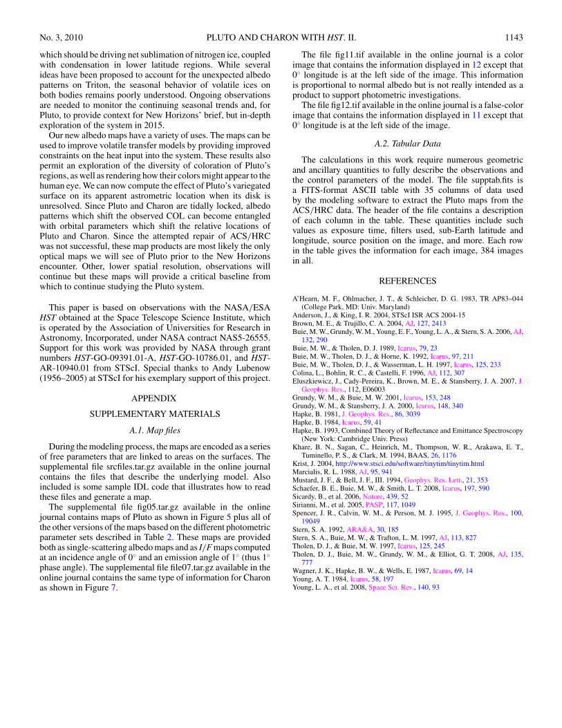
No. 3, 2010 PLUTO AND CHARON WITH HST. II. 1143
which should be driving net sublimation of nitrogen ice, coupledwith condensation in lower latitude regions. While severalideas have been proposed to account for the unexpected albedopatterns on Triton, the seasonal behavior of volatile ices onboth bodies remains poorly understood. Ongoing observationsare needed to monitor the continuing seasonal trends and, forPluto, to provide context for New Horizons’ brief, but in-depthexploration of the system in 2015.
Our new albedo maps have a variety of uses. The maps can beused to improve volatile transfer models by providing improvedconstraints on the heat input into the system. These results alsopermit an exploration of the diversity of coloration of Pluto’sregions, as well as rendering how their colors might appear to thehuman eye. We can now compute the effect of Pluto’s variegatedsurface on its apparent astrometric location when its disk isunresolved. Since Pluto and Charon are tidally locked, albedopatterns which shift the observed COL can become entangledwith orbital parameters which shift the relative locations ofPluto and Charon. Since the attempted repair of ACS/HRCwas not successful, these map products are most likely the onlyoptical maps we will see of Pluto prior to the New Horizonsencounter. Other, lower spatial resolution, observations willcontinue but these maps will provide a critical baseline fromwhich to continue studying the Pluto system.
This paper is based on observations with the NASA/ESAHST obtained at the Space Telescope Science Institute, whichis operated by the Association of Universities for Research inAstronomy, Incorporated, under NASA contract NAS5-26555.Support for this work was provided by NASA through grantnumbers HST-GO-09391.01-A, HST-GO-10786.01, and HST-AR-10940.01 from STScI. Special thanks to Andy Lubenow(1956–2005) at STScI for his exemplary support of this project.
APPENDIX
SUPPLEMENTARY MATERIALS
A.1. Map files
During the modeling process, the maps are encoded as a seriesof free parameters that are linked to areas on the surfaces. Thesupplemental file srcfiles.tar.gz available in the online journalcontains the files that describe the underlying model. Alsoincluded is some sample IDL code that illustrates how to readthese files and generate a map.
The supplemental file fig05.tar.gz available in the onlinejournal contains maps of Pluto as shown in Figure 5 plus all ofthe other versions of the maps based on the different photometricparameter sets described in Table 2. These maps are providedboth as single-scattering albedo maps and as I/F maps computedat an incidence angle of 0◦ and an emission angle of 1◦ (thus 1◦phase angle). The supplemental file file07.tar.gz available in theonline journal contains the same type of information for Charonas shown in Figure 7.
The file fig11.tif available in the online journal is a colorimage that contains the information displayed in 12 except that0◦ longitude is at the left side of the image. This informationis proportional to normal albedo but is not really intended as aproduct to support photometric investigations.
The file fig12.tif available in the online journal is a false-colorimage that contains the information displayed in 11 except that0◦ longitude is at the left side of the image.
A.2. Tabular Data
The calculations in this work require numerous geometricand ancillary quantities to fully describe the observations andthe control parameters of the model. The file supptab.fits isa FITS-format ASCII table with 35 columns of data usedby the modeling software to extract the Pluto maps from theACS/HRC data. The header of the file contains a descriptionof each column in the table. These quantities include suchvalues as exposure time, filters used, sub-Earth latitude andlongitude, source position on the image, and more. Each rowin the table gives the information for each image, 384 imagesin all.
REFERENCES
A’Hearn, M. F., Ohlmacher, J. T., & Schleicher, D. G. 1983, TR AP83–044(College Park, MD: Univ. Maryland)
Anderson, J., & King, I. R. 2004, STScI ISR ACS 2004-15Brown, M. E., & Trujillo, C. A. 2004, AJ, 127, 2413Buie, M. W., Grundy, W. M., Young, E. F., Young, L. A., & Stern, S. A. 2006, AJ,
132, 290Buie, M. W., & Tholen, D. J. 1989, Icarus, 79, 23Buie, M. W., Tholen, D. J., & Horne, K. 1992, Icarus, 97, 211Buie, M. W., Tholen, D. J., & Wasserman, L. H. 1997, Icarus, 125, 233Colina, L., Bohlin, R. C., & Castelli, F. 1996, AJ, 112, 307Eluszkiewicz, J., Cady-Pereira, K., Brown, M. E., & Stansberry, J. A. 2007, J.
Geophys. Res., 112, E06003Grundy, W. M., & Buie, M. W. 2001, Icarus, 153, 248Grundy, W. M., & Stansberry, J. A. 2000, Icarus, 148, 340Hapke, B. 1981, J. Geophys. Res., 86, 3039Hapke, B. 1984, Icarus, 59, 41Hapke, B. 1993, Combined Theory of Reflectance and Emittance Spectroscopy
(New York: Cambridge Univ. Press)Khare, B. N., Sagan, C., Heinrich, M., Thompson, W. R., Arakawa, E. T.,
Tuminello, P. S., & Clark, M. 1994, BAAS, 26, 1176Krist, J. 2004, http://www.stsci.edu/software/tinytim/tinytim.htmlMarcialis, R. L. 1988, AJ, 95, 941Mustard, J. F., & Bell, J. F., III. 1994, Geophys. Res. Lett., 21, 353Schaefer, B. E., Buie, M. W., & Smith, L. T. 2008, Icarus, 197, 590Sicardy, B., et al. 2006, Nature, 439, 52Sirianni, M., et al. 2005, PASP, 117, 1049Spencer, J. R., Calvin, W. M., & Person, M. J. 1995, J. Geophys. Res., 100,
19049Stern, S. A. 1992, ARA&A, 30, 185Stern, S. A., Buie, M. W., & Trafton, L. M. 1997, AJ, 113, 827Tholen, D. J., & Buie, M. W. 1997, Icarus, 125, 245Tholen, D. J., Buie, M. W., Grundy, W. M., & Elliot, G. T. 2008, AJ, 135,
777Wagner, J. K., Hapke, B. W., & Wells, E. 1987, Icarus, 69, 14Young, A. T. 1984, Icarus, 58, 197Young, L. A., et al. 2008, Space Sci. Rev., 140, 93