August 2017 P10/01Y/17, P12/01Y/17

Page 1 of 26

PLUME/PUFF SPREAD AND MEAN CONCENTRATION

MODULE SPECIFICATIONS

CERC

In this document ‘ADMS’ refers to ADMS 5.2, ADMS-Roads 4.1, ADMS-Urban 4.1 and

ADMS-Airport 4.1. Where information refers to a subset of the listed models, the model name is

given in full.

1. BACKGROUND TO FORMULATION

Research and field experiments have shown that the way the dispersion parameters vary with

downwind distance from a point source depends on the state of the atmospheric boundary layer

(height ), the height of the source and the height of the plume as it grows downwind. For

reviews see Hunt, Holroyd and Carruthers (1988), Hanna et al. (1989) and Weil (1985).

There is no general theory or even generally accepted semi-empirical expression that describes

the dispersion from all source heights in all conditions of the atmospheric stability (-1000

30, for Monin-Obukhov length ), and over a range of distances from the source

extending to about 30 km downwind.

The approach adopted here is first to use such formulae that have been developed, and broadly

accepted, for specific ranges of the parameters , , . We have then constructed

interpolation formulae to cover the whole range. The basis for these formulae is set out at length in

an earlier report (Hunt et al. 1988). The present model also includes a non-Gaussian model for

convective conditions not included in that report.

The broad criteria that were considered in devising these formulae and that should be used to assess

them are:

(i) The terms in the formulae should be explicable in terms of the known mechanisms of

turbulent diffusion, and therefore they can be either corrected if the mechanism is incorrect,

or improved if the mechanism becomes better understood.

(ii) The maximum mean concentration at ground level should be at least within a factor

of two of the maximum of (agreed) field measurements, and the position of maximum

should be within 50% of the measurements, and the position where the ground level

concentration should be within 50% of the measurements.

P10/01Y/17, P12/01Y/17 Page 2 of 26

An important feature of the ADMS model is that it also predicts the concentration distribution

above the ground. This enables estimates to be made of the radiation effects, chemical reaction

effects and the effects of impingement onto elevated terrain.

The distribution of the concentration profile within the boundary layer is a Gaussian plume with

reflections at the ground and at the inversion layer, if one exists, with the general form as in R91,

i.e.

(1.1)

where is the source emission rate in mass units per second and is defined as

(1.2)

The vertical dispersion parameter in the reflected Gaussian plume formula does not have a

precise definition in terms of other moments of the concentration distribution or independently

derived quantities. However, when ,

(1.3)

then the turbulence near the source defines .

In the presence of an inversion (i.e. a sharp increase in temperature with height) at the top of the

boundary layer, the plume is effectively trapped within the boundary layer. However, some

material may escape from the boundary layer due to plume rise. In this case the release is treated as

two separate plumes, within the boundary layer and in the stable region above the boundary layer.

The source strengths of the two plumes are and respectively, where is the

source strength at release and is the fraction of the plume which has penetrated the inversion.

It is assumed that in convective and neutral conditions there is always an inversion at the top of the

boundary layer. In stable conditions an inversion is only modelled if the meteorological pre-

processor predicts an inversion. If there is no inversion the release is treated as a single plume

which may spread freely out of the boundary layer.

§2 describes the dispersion parameters for stable, neutral and convective boundary layers.

§3 shows the expressions used to calculate the concentrations in the absence of plume rise or

gravitational settling while §4 describes the effects of the plume rise on , and the height of

maximum concentration, and the allowance for the effects of a finite source diameter on , . The

P10/01Y/17, P12/01Y/17 Page 3 of 26

special treatment applied in low wind conditions is described in §5. The model for a release of

finite duration (puff) is described in §6.

2. DISPERSION PARAMETERS

2.1 The Stable / Neutral Boundary Layer

All the turbulence in the stable boundary layer is mechanically generated. Usually the level of

turbulence decreases with height, as the relative damping effect of stratification increases, but it can

be enhanced from above by wave motions at the top of the boundary layer.

2.1.1 Vertical spread z

, the vertical dispersion parameter of the plume, is calculated from the vertical component

of turbulence , the travel time from the source , and buoyancy frequency , by the

relationship (Weil 1985; Hunt 1985)

(2.1)

where and are calculated at the mean plume height and are provided by the

boundary layer structure module, and the parameter b is given by

(2.2)

In plumes originating near ground level, 0.1, mean velocity shear plays a significant

role in their dispersion; a linear interpolation is used in the range 0.05 0.15 in

order to obtain a smooth transition between 0.1 and 0.1. In addition, once

has reached 1 it remains at 1. Note that throughout this analysis and are related by

where is the local wind speed evaluated at .

2.1.2 Transverse Spread y

The transverse dispersion parameter, , is given by

(2.3a)

with

P10/01Y/17, P12/01Y/17 Page 4 of 26

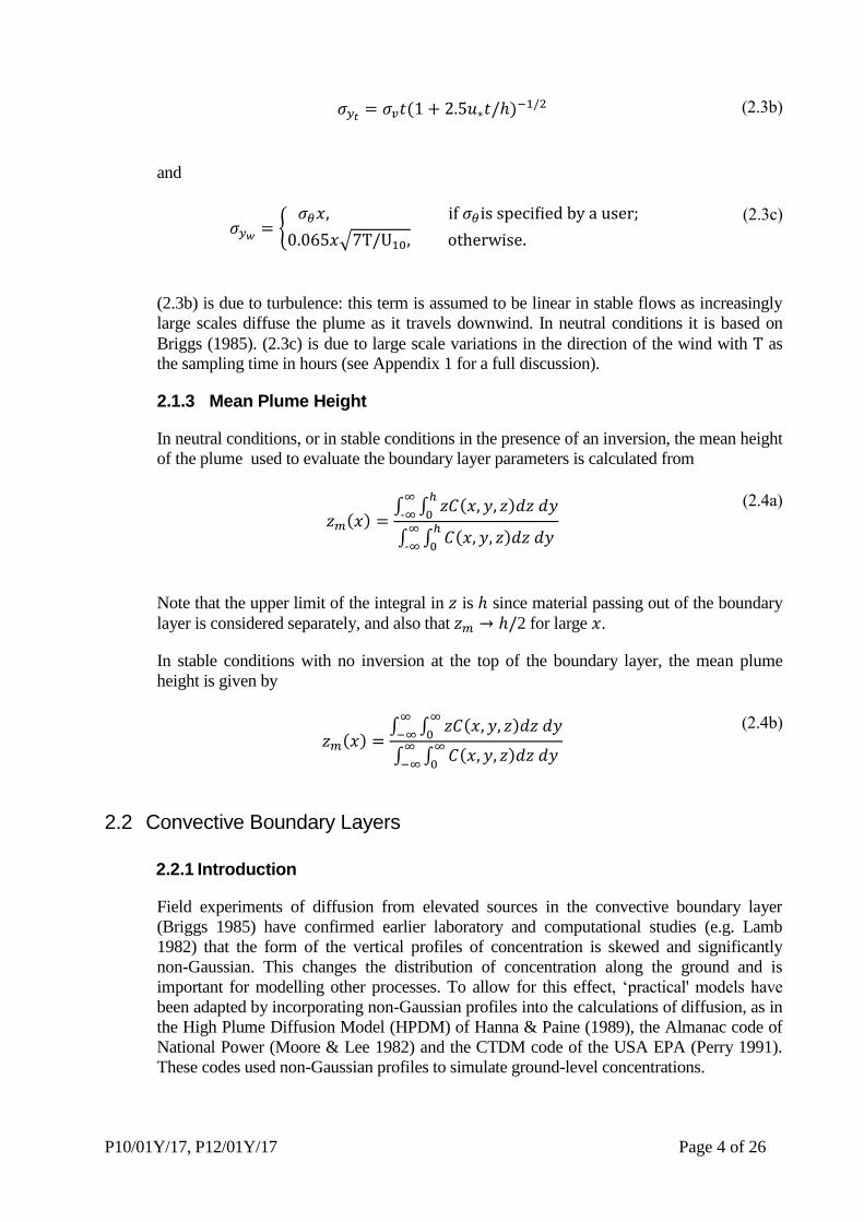
(2.3b)

and

(2.3c)

(2.3b) is due to turbulence: this term is assumed to be linear in stable flows as increasingly

large scales diffuse the plume as it travels downwind. In neutral conditions it is based on

Briggs (1985). (2.3c) is due to large scale variations in the direction of the wind with as

the sampling time in hours (see Appendix 1 for a full discussion).

2.1.3 Mean Plume Height

In neutral conditions, or in stable conditions in the presence of an inversion, the mean height

of the plume used to evaluate the boundary layer parameters is calculated from

(2.4a)

Note that the upper limit of the integral in is since material passing out of the boundary

layer is considered separately, and also that 2 for large .

In stable conditions with no inversion at the top of the boundary layer, the mean plume

height is given by

(2.4b)

2.2 Convective Boundary Layers

2.2.1 Introduction

Field experiments of diffusion from elevated sources in the convective boundary layer

(Briggs 1985) have confirmed earlier laboratory and computational studies (e.g. Lamb

1982) that the form of the vertical profiles of concentration is skewed and significantly

non-Gaussian. This changes the distribution of concentration along the ground and is

important for modelling other processes. To allow for this effect, ‘practical' models have

been adapted by incorporating non-Gaussian profiles into the calculations of diffusion, as in

the High Plume Diffusion Model (HPDM) of Hanna & Paine (1989), the Almanac code of

National Power (Moore & Lee 1982) and the CTDM code of the USA EPA (Perry 1991).

These codes used non-Gaussian profiles to simulate ground-level concentrations.

P10/01Y/17, P12/01Y/17 Page 5 of 26

2.2.2 Vertical Spread

In the convective boundary layer (CBL) the probability density function (p.d.f.) of the

vertical velocity is non-Gaussian. Near the source particles travel in

straight lines from the source where is the Lagrangian time scale. Then the

probability of a particle being at a height at time after its release is where . The proportionality factor is determined by

normalising the pdfs. Recall that for a continuous line source release of strength (from

Hunt 1985, or van Dop & Nieuwstadt 1982)

(2.5)

(which satisfies

,

1; where = release rate per unit length,

denotes the crosswind-integrated concentration from an isolated source with release rate

). Thence

(2.6)

Note that if is Gaussian,

(2.7)

then

(2.8)

where

(2.9)

A non-Gaussian p.d.f. for the vertical velocity in thermal convection is, following Hunt,

Kaimal & Gaynor (1988) (to be referred to as HKG),

(2.10)

where are step functions, , is the mode, and , , , define

the p.d.f.s for the upward and downward velocities. Note that in the CBL it is typically

found that 0, .

P10/01Y/17, P12/01Y/17 Page 6 of 26

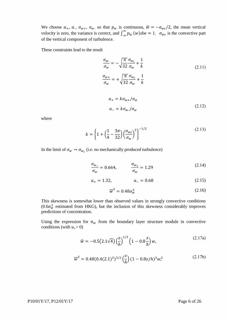
We choose , , , so that is continuous, the mean vertical

velocity is zero, the variance is correct, and

1. is the convective part

of the vertical component of turbulence.

These constraints lead to the result

(2.11)

(2.12)

where

(2.13)

In the limit of (i.e. no mechanically produced turbulence)

(2.14)

(2.15)

(2.16)

This skewness is somewhat lower than observed values in strongly convective conditions

(0.6 estimated from HKG), but the inclusion of this skewness considerably improves

predictions of concentration.

Using the expression for from the boundary layer structure module in convective

conditions (with = 0)

(2.17a)

(2.17b)

P10/01Y/17, P12/01Y/17 Page 7 of 26

2.2.3 Decorrelation of Vertical Velocity

Allowance is made for this by replacing occurrences of in the expressions for

concentration by

(2.18)

where is the Lagrangian timescale. Hence the vertical spread is given by

(2.19)

2.2.4 Transverse Spread

The transverse dispersion parameter is calculated from two parts (derived from Briggs,

1985), the first for dispersion due to convection , the second due to mechanically driven

turbulence , which is identical to (2.3b) above.

(2.20)

(2.21)

An additional term (2.3c) is also included to allow for variation in the wind direction.

2.2.5 Mean plume height

In convective conditions the mean plume height is calculated using the same expression as

for neutral conditions, equation (2.4a).

2.3 Above the boundary layer

2.3.1 Vertical spread z

Above the boundary layer the vertical spread is given by

(2.22)

where is the travel time from the source, is the buoyancy frequency above the boundary

layer and is calculated at the mean plume height by the boundary layer structure module.

P10/01Y/17, P12/01Y/17 Page 8 of 26

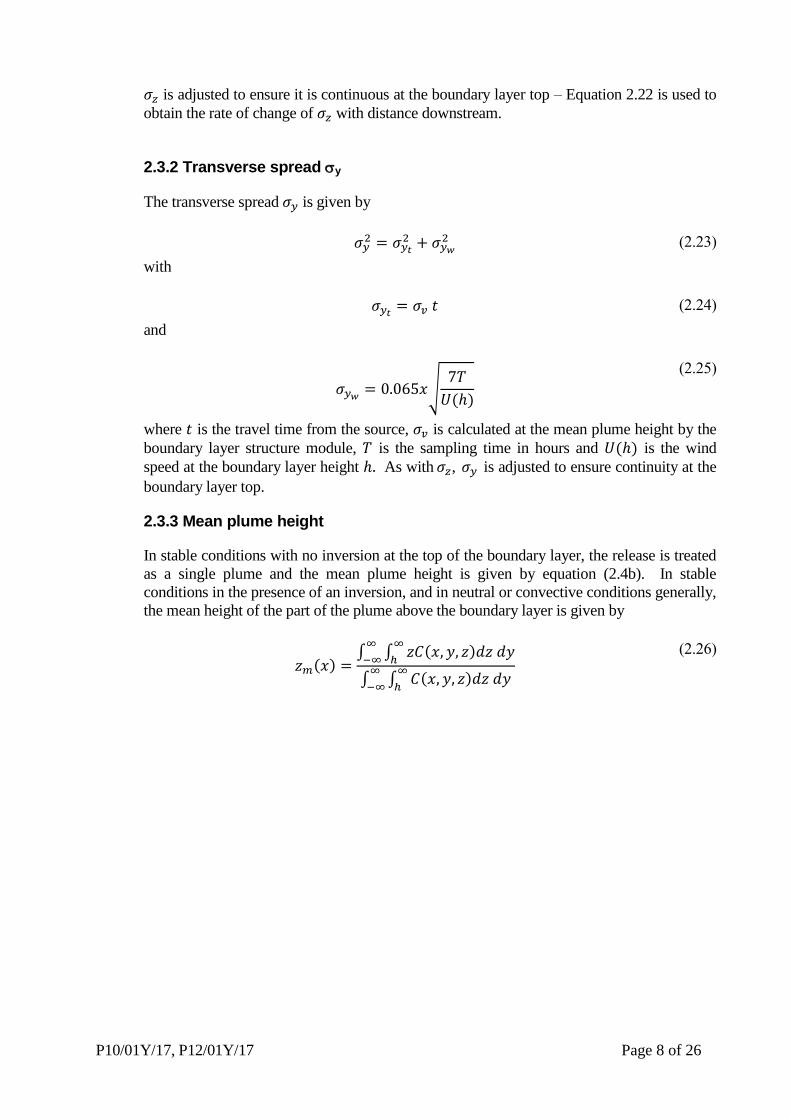
is adjusted to ensure it is continuous at the boundary layer top – Equation 2.22 is used to

obtain the rate of change of with distance downstream.

2.3.2 Transverse spread y

The transverse spread is given by

(2.23)

with

(2.24)

and

(2.25)

where is the travel time from the source, is calculated at the mean plume height by the

boundary layer structure module, is the sampling time in hours and is the wind

speed at the boundary layer height As with , is adjusted to ensure continuity at the

boundary layer top.

2.3.3 Mean plume height

In stable conditions with no inversion at the top of the boundary layer, the release is treated

as a single plume and the mean plume height is given by equation (2.4b). In stable

conditions in the presence of an inversion, and in neutral or convective conditions generally,

the mean height of the part of the plume above the boundary layer is given by

(2.26)

P10/01Y/17, P12/01Y/17 Page 9 of 26

3. MEAN CONCENTRATION

3.1 The use of near-field and far-field models

In the presence of an inversion at the top of the boundary layer, the plume is effectively confined

within the boundary layer because material reaching the top of the layer is reflected downwards

(except that plume rise results in a fraction escaping from the boundary layer, which is considered

as a separate plume). Sufficiently far from the source after parts of the plume have been reflected at

the ground, the top of the boundary layer, and possibly at both, the vertical variation in

concentration of the pollutant is so small as to be negligible, approximately where . Then

the plume can be considered to grow horizontally as a vertical wedge rather than as a cone. Upwind

and downwind of this point different models are used which are referred to as the near-field and

far-field models.

In stable conditions, providing there is no inversion, the plume is assumed to continue growing

downstream as a cone indefinitely.

3.2 The Near-field model – Stable / Neutral Boundary Layer h/LMO -0.3

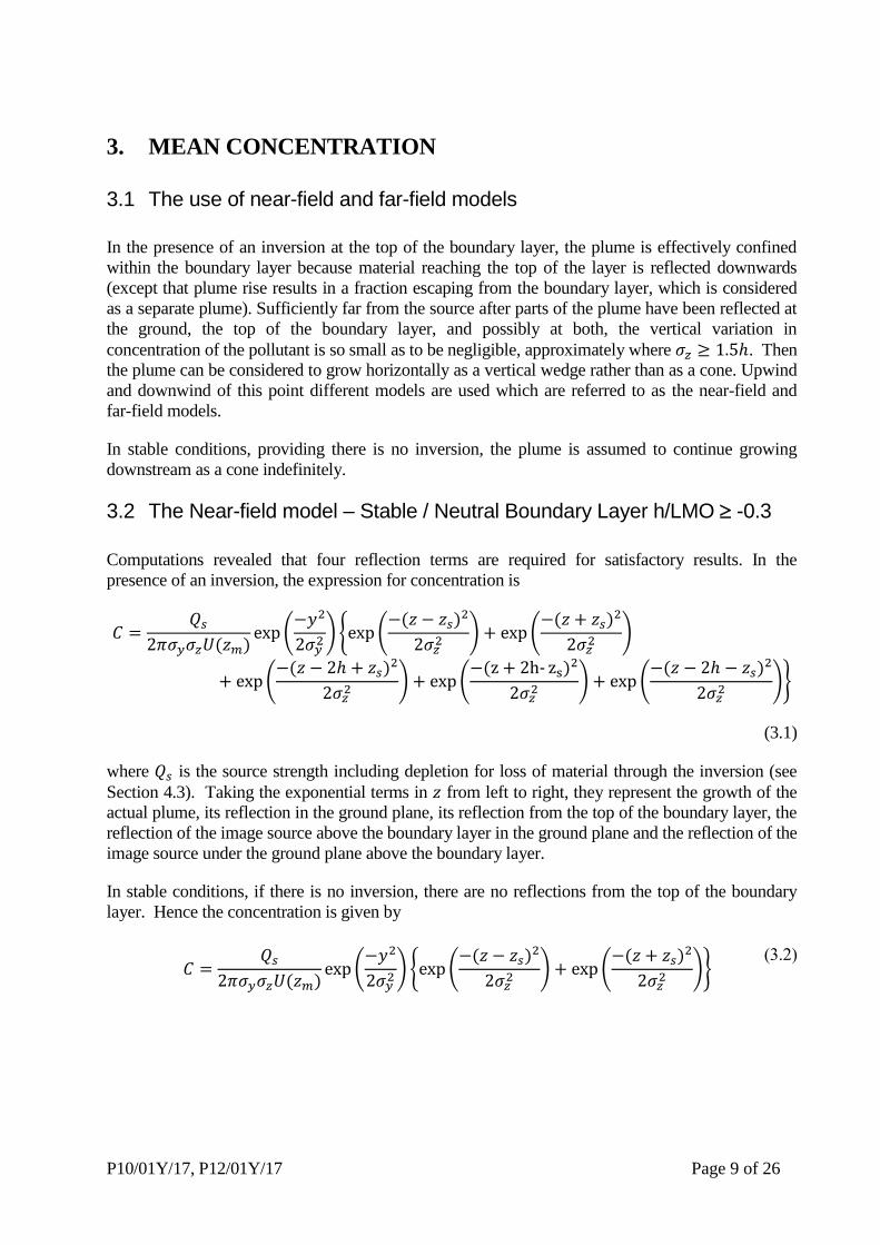
Computations revealed that four reflection terms are required for satisfactory results. In the

presence of an inversion, the expression for concentration is

(3.1)

where is the source strength including depletion for loss of material through the inversion (see

Section 4.3). Taking the exponential terms in from left to right, they represent the growth of the

actual plume, its reflection in the ground plane, its reflection from the top of the boundary layer, the

reflection of the image source above the boundary layer in the ground plane and the reflection of the

image source under the ground plane above the boundary layer.

In stable conditions, if there is no inversion, there are no reflections from the top of the boundary

layer. Hence the concentration is given by

(3.2)

P10/01Y/17, P12/01Y/17 Page 10 of 26

3.3 The Near-field model - Convective boundary layer h/LMO < -0.3

The convective formulation for concentration in the near-field is

(3.3)

where

(3.4)

3.4 The Far-field model

When the plume fills the boundary layer and grows horizontally like a vertical wedge the dispersion

is similar to that from a vertical line source, the chief difference being that the wind speed varies

along the line. Transition to the far-field model is effected when . To allow the standard

P10/01Y/17, P12/01Y/17 Page 11 of 26

expressions for dispersion from a line source to be used for far-field dispersion, the wind speed at

the mid-height of the boundary layer, , is used so that the concentration is given by

(3.5)

for both stable and convective layers. This may be regarded as a reasonable approximation for the

concentration in the far field. Matching at the transition is achieved simply by matching the

concentration at the surface below the plume centreline. This defines an adjusted source strength

. Because when the vertical concentration is not completely uniform and some

material is lost due to using only four reflection terms, there is a small difference between and

. These are brought into line by a smooth transition over the range

(3.6)

where when , whereby for all .

3.5 Above the boundary layer

In stable conditions, providing there is no inversion at the top of the boundary layer, the plume may

freely spread above the boundary layer and the concentration is given by equation (3.2). In the

presence of an inversion, or in neutral or convective conditions, the concentration due to a plume

above the boundary layer is given by

(3.7)

Concentrations above the boundary layer are only output for ADMS 5.

P10/01Y/17, P12/01Y/17 Page 12 of 26

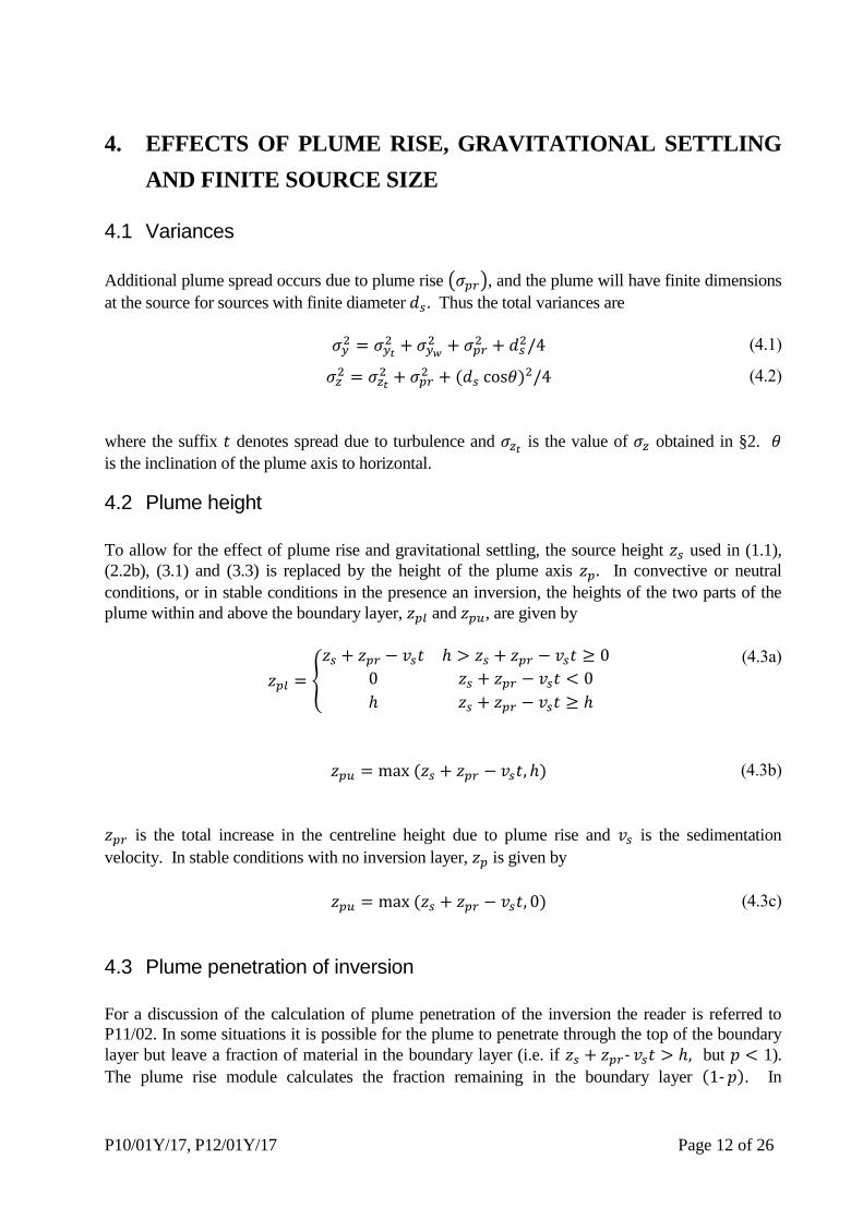
4. EFFECTS OF PLUME RISE, GRAVITATIONAL SETTLING

AND FINITE SOURCE SIZE

4.1 Variances

Additional plume spread occurs due to plume rise , and the plume will have finite dimensions

at the source for sources with finite diameter . Thus the total variances are

(4.1)

(4.2)

where the suffix denotes spread due to turbulence and is the value of obtained in §2.

is the inclination of the plume axis to horizontal.

4.2 Plume height

To allow for the effect of plume rise and gravitational settling, the source height used in (1.1),

(2.2b), (3.1) and (3.3) is replaced by the height of the plume axis In convective or neutral

conditions, or in stable conditions in the presence an inversion, the heights of the two parts of the

plume within and above the boundary layer, and , are given by

(4.3a)

(4.3b)

is the total increase in the centreline height due to plume rise and is the sedimentation

velocity. In stable conditions with no inversion layer, is given by

(4.3c)

4.3 Plume penetration of inversion

For a discussion of the calculation of plume penetration of the inversion the reader is referred to

P11/02. In some situations it is possible for the plume to penetrate through the top of the boundary

layer but leave a fraction of material in the boundary layer (i.e. if but 1).

The plume rise module calculates the fraction remaining in the boundary layer . In

P10/01Y/17, P12/01Y/17 Page 13 of 26

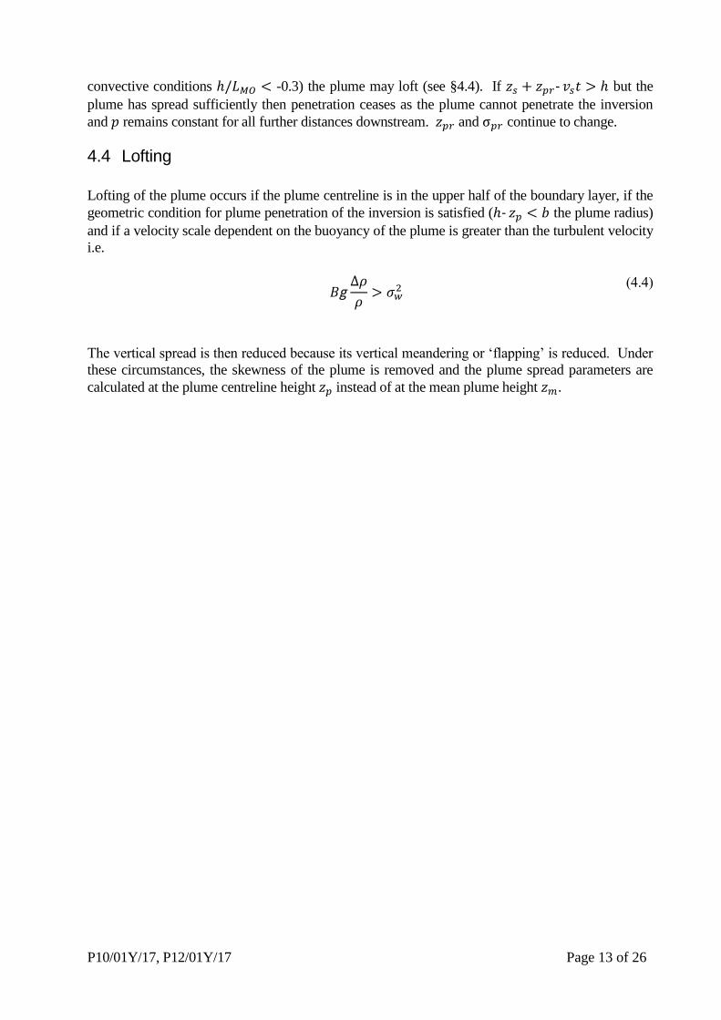
convective conditions -0.3) the plume may loft (see §4.4). If but the

plume has spread sufficiently then penetration ceases as the plume cannot penetrate the inversion

and remains constant for all further distances downstream. and continue to change.

4.4 Lofting

Lofting of the plume occurs if the plume centreline is in the upper half of the boundary layer, if the

geometric condition for plume penetration of the inversion is satisfied ( the plume radius)

and if a velocity scale dependent on the buoyancy of the plume is greater than the turbulent velocity

i.e.

(4.4)

The vertical spread is then reduced because its vertical meandering or ‘flapping’ is reduced. Under

these circumstances, the skewness of the plume is removed and the plume spread parameters are

calculated at the plume centreline height instead of at the mean plume height .

P10/01Y/17, P12/01Y/17 Page 14 of 26

5. SPECIAL TREATMENT IN LOW WIND CONDITIONS

5.1 Introduction

For lower mean wind speeds the direction of the wind becomes more variable. In very unstable

conditions this can arise because the turbulent fluctuations in the flow are large or comparable

with the mean wind even when the geostrophic wind is well defined. In stable conditions when

the geostrophic wind is very small both the mean and turbulent wind can be very small and

immeasurable, but more usually the measured wind at the surface is very light either with

variable direction or with consistent direction with the wind being forced by thermal gradients or

topography.

The standard ADMS calculations already account for large scale variations in the direction of the

wind in the calculation of the transverse spread,

, as described by equation

(2.3c).

The approach used in ADMS 5 for low wind conditions (when activated by the user through an

‘.aai’ file) is to calculate the concentration as a weighted average of a ‘Gaussian’ type plume

(incorporating if entered by the user) and a radially symmetric plume . In ADMS-

Roads, ADMS-Urban and ADMS-Airport low wind speeds are increased to a minimum value of

0.75 m/s at 10 m, where the Gaussian solution remains valid, so a calm solution is not required.

5.2 Calculation of the radially symmetric plume concentration Cr

The ‘radial’ plume is modelled as a passive release, with a source height determined by the

maximum plume height from the normal plume rise calculations. If the wind speed at 10 m is

below a threshold value , by default 0.5 m/s, no ‘gaussian’ concentration is calculated, but

the normal plume rise calculations are still carried out in order to establish the source height for

the radial source.

The general form of the equation for is (1.1) with the dependence on y removed, and

replaced by in the denominator as follows:

(5.1)

5.3 Calculation of concentration C as a weighted average of Cg and Cr

We define conditions for switching on the weighting depending on whether the magnitude of the

observed mean wind at 10 m ( ) is greater than a combination of a threshold wind speed

P10/01Y/17, P12/01Y/17 Page 15 of 26

and the ratio of to the tendency for the turbulence to diffuse in the

longitudinal direction

where is the root-mean-squared longitudinal velocity,

the time from release and the Lagrangian time scale.

The weighting is switched on when

where

(5.2)

The time variable is calculated at the mean plume height, which can be justified by saying that

is the critical wind speed value calculated directly beneath the plume centreline at time and height 10 m.

The weighted average is calculated as follows:

(5.3)

where , and

take the following default values:

1.0 m/s

0.5 m/s

0.3 m/s

If is less than then it is re-set to

; and are revised accordingly.

P10/01Y/17, P12/01Y/17 Page 16 of 26

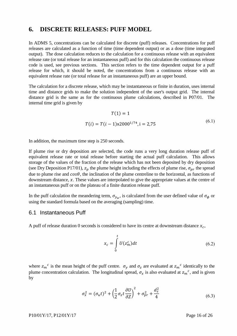
6. DISCRETE RELEASES: PUFF MODEL

In ADMS 5, concentrations can be calculated for discrete (puff) releases. Concentrations for puff

releases are calculated as a function of time (time dependent output) or as a dose (time integrated

output). The dose calculation reduces to the calculation for a continuous release with an equivalent

release rate (or total release for an instantaneous puff) and for this calculation the continuous release

code is used, see previous sections. This section refers to the time dependent output for a puff

release for which, it should be noted, the concentrations from a continuous release with an

equivalent release rate (or total release for an instantaneous puff) are an upper bound.

The calculation for a discrete release, which may be instantaneous or finite in duration, uses internal

time and distance grids to make the solution independent of the user's output grid. The internal

distance grid is the same as for the continuous plume calculations, described in P07/01. The

internal time grid is given by

(6.1)

In addition, the maximum time step is 250 seconds.

If plume rise or dry deposition are selected, the code runs a very long duration release puff of

equivalent release rate or total release before starting the actual puff calculation. This allows

storage of the values of the fraction of the release which has not been deposited by dry deposition

(see Dry Deposition P17/01), the plume height including the effects of plume rise, the spread

due to plume rise and , the inclination of the plume centreline to the horizontal, as functions of

downstream distance, . These values are interpolated to give the appropriate values at the centre of

an instantaneous puff or on the plateau of a finite duration release puff.

In the puff calculation the meandering term, , is calculated from the user defined value of or

using the standard formula based on the averaging (sampling) time.

6.1 Instantaneous Puff

A puff of release duration 0 seconds is considered to have its centre at downstream distance ,

(6.2)

where is the mean height of the puff centre. and are evaluated at

identically to the

plume concentration calculation. The longitudinal spread, is also evaluated at , and is given

by

(6.3)

P10/01Y/17, P12/01Y/17 Page 17 of 26

The second term on the right hand side of the equation represents the longitudinal spread due to

shear (Hunt 1982, p266).

Concentrations are given by

(6.4)

in neutral conditions, or in stable conditions in the presence of an inversion (cf equation (3.1)),

where is the total mass released.

For convective conditions, stable conditions with no inversion, or a puff above the boundary layer,

the expression in curly brackets and the term are replaced by the convective solution in equation

(3.3), the stable solution in equation (3.2) or the above boundary layer solution in equation (3.5) as

appropriate. includes the effect of plume rise and gravitational settling, as for the plume, §4.2.

6.2 Finite release duration puff

The finite release starts at time and finishes at Then, at time the "front" of the puff is at

where

(6.5)

and the "rear" of the puff at time is at , where

(6.6)

P10/01Y/17, P12/01Y/17 Page 18 of 26

and

are the mean height of the puff front and rear. There are non-zero concentrations

ahead of and downstream of , due to the longitudinal spreading, which is given by

(6.7)

(6.8)

the parameters in (6.7) being evaluated at , the mean height of the front of the puff, and those in

(6.8) being evaluated at .

An effective front and rear of the puff are defined by

(6.9)

(6.10)

where is chosen to satisfy mass continuity, so that the mass of emitted material in is equal

to the mass of emitted material depleted from .

Using a normal distribution, 1.25.

It is now possible to define the 3 regimes of the puff which are treated in the code. These are

(i) A front end with concentration given by

(6.11)

(ii) The "plateau" region where the concentrations are identical to those

obtained from a plume with the equivalent emission rate. Here the longitudinal gradients of

mean concentrations are caused only by dispersion in vertical and transverse directions.

This region is eroded by longitudinal dispersion which spreads regions (i) and (iii). and

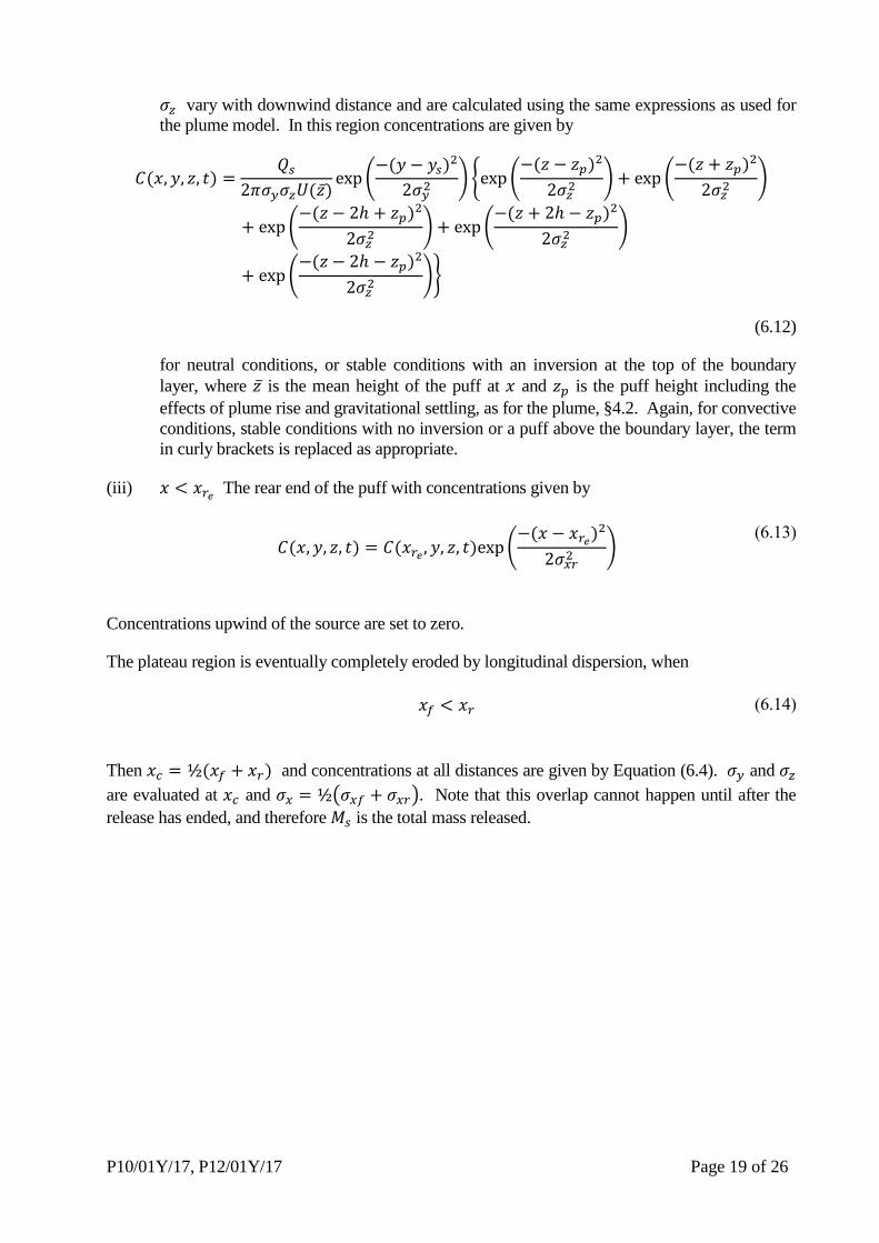
P10/01Y/17, P12/01Y/17 Page 19 of 26

vary with downwind distance and are calculated using the same expressions as used for

the plume model. In this region concentrations are given by

(6.12)

for neutral conditions, or stable conditions with an inversion at the top of the boundary

layer, where is the mean height of the puff at and is the puff height including the

effects of plume rise and gravitational settling, as for the plume, §4.2. Again, for convective

conditions, stable conditions with no inversion or a puff above the boundary layer, the term

in curly brackets is replaced as appropriate.

(iii) The rear end of the puff with concentrations given by

(6.13)

Concentrations upwind of the source are set to zero.

The plateau region is eventually completely eroded by longitudinal dispersion, when

(6.14)

Then and concentrations at all distances are given by Equation (6.4). and

are evaluated at and . Note that this overlap cannot happen until after the

release has ended, and therefore is the total mass released.

P10/01Y/17, P12/01Y/17 Page 20 of 26

REFERENCES

Briggs, G.A. (1985) Analytical parameterizations of diffusion: the convective boundary layer.

J. Clim. Appl. Met. 14, 1167-1186.

Deardorff, J.W. & Willis, G.E. (1975) A parameterization of diffusion into a mixed layer. J. Appl.

Met. 14, 1451-1458.

Doran, J.C., Horst, T. and Nickola P. (1978) Experimental observation of the dependence of lateral

and vertical characteristics on source height. Atmos. Env. 12, 2259-2263.

Hanna, S.R. & Paine, R.J. (1989) Hybrid plume dispersion model (HPDM) development and

evaluation. J. Appl. Meteorol., 28, 206-224.

Hunt, J.C.R. (1982) Diffusion in the stable boundary layer. In Atmospheric Turbulence and Air

Pollution Modelling (eds. F.T.M. Nieuwstadt & A. van Dop), 238pp. D. Reidel, Dordrecht.

Hunt, J.C.R. (1985) Turbulent diffusion from sources in complex flows. Ann. Rev. Fluid Mech., 17,

447-458.

Hunt, J.C.R., Holroyd, R.J. & Carruthers, D.J. (1988) Preparatory studies for a complex dispersion

model. Report to NRPB.

Hunt, J.C.R., Kaimal, J.C. & Gaynor, J.E. (1988) Eddy structure in the convective boundary layer -

new measurements and new concepts. Q.J.R. Meteorol. Soc., 114, 827-858.

Hunt, J.C.R. & Weber, A.H. (1979) A Lagrangian statistical analysis of diffusion from a ground

level source in a turbulent boundary layer. Q.J. Roy. Met. Soc. 105, 423-443.

Lamb, R.G. (1982) Diffusion in the convective boundary layer. In Atmospheric Turbulence and Air

Pollution Modelling (eds. F.T.M. Nieuwstadt \& H. van Dop), pp.159-230. D. Reidel, Dordrecht.

Lenschow, D.H. & Stephens, P.L. (1980) The role of thermals in the convective boundary layer.

Boundary-layer Meteorol., 19, 519-532.

Moore, D.J. & Lee, B.Y. (1982) An asymmetrical Gaussian plume model. Central Electricity

Generating Board Report, RD/L/2224N81.

Perry (1991) CTDMPLUS: A dispersion model for sources near complex topography. Part I:

Technical formulations.

Venkatram, A., Strimaitis, D.G. and Dicristofaro, D. (1984) A semi-empirical model to estimate

vertical dispersion of elevated releases in the stable boundary layer. Atmos. Env. 18, 923-928.

Weil, J.C. 1985. Updating applied diffusion models. J. Clim. Appl. Met. 24, 1111-1130.

P10/01Y/17, P12/01Y/17 Page 21 of 26

APPENDIX 1

MODELLING LATERAL DISPERSION

by

A. G. Robins

SUMMARY

This appendix discusses the form and applicability of the model for lateral spread. This contains

two terms, one due to boundary layer turbulence and the other to wind direction unsteadiness.

Attention is focused on the latter, for which two models are given, one based on local wind

direction measurements and the other a generic model for the United Kingdom.

1. INTRODUCTION

The boundary layer depth generally limits the size of the largest eddies which influence vertical

dispersion. However, the same cannot be said for lateral dispersion in the atmosphere as there is a

continuous range of 'eddy' sizes, from local to weather system scales, which affect the statistics of

the horizontal wind component. We generally view this in terms of two components, one the

boundary layer turbulence, and the other wind direction unsteadiness. The two components are

assumed to be independent. In special circumstances, for example in the laboratory, only the

former exists, and both the lateral and vertical eddy scales are limited simply by the boundary layer

depth.

Because of the relatively unlimited range of horizontal eddy sizes in the atmosphere, lateral spread

is a function of the period over which it is observed. This presents problems for, although the

boundary layer turbulence component can be modelled in a universal manner, wind direction

unsteadiness reflects local climatic conditions. In general, the latter can only be represented by

ensemble average statistics, implying that resulting spread predictions are also for ensemble

averages.

The model for lateral spread is described in the following section. Two options are given for the

wind direction unsteadiness component, one based on local wind field measurements and the other

a generic model for the United Kingdom. The latter should also be a reasonable model for north-

west maritime Europe and could be adapted for other regions.

P10/01Y/17, P12/01Y/17 Page 22 of 26

2. THE DISPERSION MODEL

Following Moore (1976), we model lateral spread, , in terms of a boundary layer turbulence

component, suffix , and a wind direction unsteadiness component, suffix , as:

(1)

The model for the first of the components is described in Carruthers et al (1992). The second is

evaluated from either of the following:

(2)

(3)

where is the (user-specified) standard deviation of the horizontal wind direction, the

downstream distance from the source, the required averaging time (in hours) for evaluating

lateral spread and the average ten metre wind speed over the same period. Bennett (1980)

analysed hourly wind direction records and showed that the second of the above expressions

remains valid for 24 hours. Above the boundary layer, the wind speed at the boundary layer

top is used in place of .

As specified by Moore, the turbulence term, , is related to a three minute averaging period, in

common with Pasquill's early work (e.g. see Pasquill and Smith, 1983), so the full definition of

should stipulate that it is averaged over consecutive three minute periods and sampled over the

plume spread averaging time, . In principle, any sensible period could be chosen to separate the

two components of lateral spread, and the above definitions suitably amended.

Equation (3) was developed by Moore from dispersion measurements in the United Kingdom over

fetches up to about 15 km. It is also supported by analysis of wind direction records (Bennett,

1980). In common with other models (e.g. Clarke, 1979), we take a simple linear extrapolation to

all distances of interest (in this case 30 km). This assumes that the effective integral scale of the

wind direction fluctuations, , is so large that over all distances of interest - a

reasonable assumption in the present circumstances.

The generalisation of (3) is:

(4)

where is a constant, the annual average 10 metre wind speed, and a reference time

period.

P10/01Y/17, P12/01Y/17 Page 23 of 26

3. DERIVATION OF THE MODEL

Moore (1969) analysed extensive measurements of dispersion within about 15 km of tall stacks and

concluded that the full hourly average lateral spread could be fitted by:

(5)

though there was a tendency for to decrease with increasing wind speed. Simultaneous

meteorological measurement from a nearby tall tower showed that the intensity of lateral turbulence

at a height of about 100 m fell from about 16%, at a wind speed of around 1 ms-1

, to about 5%, at

16 ms-1

or above. On this basis Moore (1974) proposed a simple generalisation of (5):

(6)

which was further generalised for any averaging period to:

(7)

The last step was to include the role of boundary layer turbulence by splitting (7) into two terms,

resulting in equations (1) and (3) above.

Bennett (1980) subsequently analysed (3) on the basis of long term records of hourly horizontal

wind velocity and showed that the expression was supported for averaging times up to 24 hours.

P10/01Y/17, P12/01Y/17 Page 24 of 26

4. FURTHER DISCUSSION

The model applies to dispersion under the following conditions:

a. homogeneous, level terrain

b. steady, homogeneous meteorological conditions

c. no spread due to relative motion

The first should be satisfied over an area of linear dimensions significantly greater than the largest

source-receptor fetch of interest, particularly upwind from the source. The second should hold over

a time scale greater than the sum of the travel time and the averaging time. The final condition

implies that the emission is passive. In other cases relative motion will occur between the plume

and the ambient flow (e.g. due to plume rise) and additional spread will result. This is represented

in the plume rise model and need not be discussed in the present context.

Individual realisations of a concentration field are not generally Gaussian-like in nature, reflecting

the nature of wind direction fluctuations and the structure of boundary layer turbulence (if is

short enough). This feature of the dispersion problem is not treated in ADMS, which predicts only

ensemble averaged statistics of the concentration field. In keeping with this, the lateral spread

model only describes ensemble averaged dispersion, no matter what the emission duration.

Concentration fluctuation predictions can be modelled if the structure of the velocity fluctuations is

known. Consequently, in ADMS 5, this is restricted to the boundary layer turbulence component

and hence only fluctuations on relatively short time scales (less than 1 hour) are predicted.

The formula for combining the two terms contributing to the lateral spread assumes that each is an

independent Gaussian process. It seems likely that this is only partially true, the lateral turbulence

being Gaussian, though the resulting errors do not appear to be significant. However, it must be

emphasised that, because of limited experimental information, the lateral spread model has not been

exhaustively tested.

P10/01Y/17, P12/01Y/17 Page 25 of 26

5. APPLICATION

5.1 Dispersion in the United Kingdom

The model has been derived and tested under UK meteorological conditions. In general, the upper

limit for is 24 hours, though a smaller value may be appropriate in very light winds to avoid the

prediction of excessive rates of lateral spread. A sensible limit is:

(6)

The model is applicable to continuous releases and short duration releases, where becomes the

release duration. In the latter case, the mean wind direction is defined over the release duration.

The contribution of the wind direction unsteadiness terms to the lateral dispersion of very short

duration emissions (puffs) is negligible in this framework. However, puff dispersion might be

required in a framework in which the mean wind direction is defined over some non-zero period

(e.g. 1 hour). is then the period used for defining the mean wind.

The underlying meteorological conditions must remain essentially steady over the period

5.2 Dispersion in Other Regions

The applicability of the model depends on which of the two methods is used to predict . In the

first case, long running wind direction measurements are needed to define and the model can

then be used as for UK applications. The second method may be a reasonable model for north west

maritime Europe, though in general local data will be necessary to define the model constants.

REFERENCES

Bennett, M. (1980) Plume spread due to changing synoptic winds: analysis of wind records. CEGB

Memorandum LM/PHYS/196.

Carruthers, D.J., Weng, W.S., Hunt, J.C.R. and Holroyd, R.J. (1992) Plume/puff spread and mean

concentration module specifications. UK-ADMS Paper UK-ADMS1.0 P10&12/01F/92.

Clarke, R.H. (1979) A model for short and medium range dispersion of radionuclides released into

the atmosphere. NRPB Report NRPB-R91.

Moore, D.J. (1969) The distribution of surface concentrations of sulphur dioxide emitted from a tall

chimney. Phil. Trans. R. Soc. London Ser A 265, 245-259.

Moore, D.J. (1974) Observed and calculated magnitudes and distances of maximum ground level

concentration of gaseous effluent material downwind of a tall stack. Adv. Geophys. 18B, 201-221.

P10/01Y/17, P12/01Y/17 Page 26 of 26

Moore, D.J. (1976) Calculation of ground level concentration for different sampling periods and

source locations. Atmospheric Pollutions, Elsevier, Amsterdam, 5160.

Pasquill, F. and Smith, F.B. (1983) Atmospheric diffusion. Ellis Horwood, Chichester.