Embed Size (px)
Citation preview
Plug Formation and Dissociation of Mixed Gas Hydrates and Methane Semi-Clathrate Hydrate Stability
A thesis submitted in partial fulfilment of the requirements for the degree
of Doctor of Philosophy
in Chemical and Process Engineering
by Thomas John Hughes
UNIVERSITY OF CANTERBURY
2008
ii
ABSTRACT
Gas hydrates are known to form plugs in pipelines. Hydrate plug dissociation times can be
predicted using the CSMPlug program. At high methane mole fractions of a methane +
ethane mixture the predictions agree with experiments for the relative dissociation times of
structure I (sI) and structure II (sII) plugs. At intermediate methane mole fractions the
predictions disagree with experiment. Enthalpies of dissociation were measured and
predicted with the Clapeyron equation. The enthalpies of dissociation for the methane +
ethane hydrates were found to vary significantly with pressure, the composition, and the
structure of hydrate. The prediction and experimental would likely agree if this variation in
the enthalpy of dissociation was taken in to account.
In doing the plug dissociation studies at high methane mole fraction a discontinuity was
observed in the gas evolution rate and X-ray diffraction indicated the possibility of the
presence of both sI and sII hydrate structures. A detailed analysis by step-wise modelling
utilising the hydrate prediction package CSMGem showed that preferential enclathration
could occur. This conclusion was supported by experiment.
Salts such as tetraisopentylammonium fluoride form semi-clathrate hydrates with melting
points higher than 30 °C and vacant cavities that can store cages such as methane and
hydrogen. The stability of this semi-clathrate hydrate with methane was studied and the
dissociation phase boundary was found to be at temperatures of about (25 to 30) K higher
than that of methane hydrate at the same pressure.

iii
ACKNOWLEDGEMENTS
Firstly I would like to sincerely thank Professor Ken Marsh, there have been highs and lows
during this project, thank you for always supporting and encouraging me, your thirst for
knowledge and enthusiasm are an inspiration. I hope you will have more time to enjoy your
retirement now.
I would also like to thank Associate Professor John Abrahamson and Professor Alan Mather
for supervising me. Thank you for taking the time to show an interest in my work and
helping me out when I needed it.
I also wish to express gratitude to Professor E. Dendy Sloan for hosting and supervising me
for a period of study at the Center for Hydrate Research at the Colorado School of Mines. It
was a great privilege to be in the presence of such a well-renown expert and the knowledge
that I gained during my time at CSM was immeasurable helpful in the completion of this
work. I would also like to thank Professor Carolyn Koh for her thoughts and suggestions,
Simon Davies and Keith Hester for helping me with measurements, and John Boxall for
finding somewhere so convenient to stay.
I am also most obliged to Emeritus Professor Ward Robinson and Dr. Jan Wikaira from the
Chemistry department for helping me with X-ray diffraction measurements. A thanks also
goes to Dr. Marie Squire for collecting my NMR spectra and to Dr. John Smaill from
Mechanical Engineering for checking my pressure cell designs.
I have had a great deal of technical assistance during this project and wish to thank all the
technical staff for their help. I would particularly like to thank Frank Weerts for the
construction of my pressure cells, Mike Lahood, Slywester Zwolinski, and Tim Moore for
running electrical tests and diagnostic repairs on the ever unreliable DSC, and Tony Allen for
assisting in the set up of data acquisition and computer logging hardware. I would also like to
thank Leigh Richardson for the construction of a crate for shipping the DSC and Glenn
Wilson for ordering and purchasing parts and materials for my work. Trevor Berry also

iv
deserves a special mention, for always finding the parts and equipment I needed and for
teaching me how to use the gas chromatograph.
This work would not have been possible without funding from the Gas Processors
Association (GPA); I offer them my appreciation and thanks. I would also like to thank my
project’s GPA research committee for their patience and understanding.
Finally I wish to thank my family and friends for supporting me throughout this project. I
would like to especially thank my parents for bringing me countless cups of tea and coffee
during the long process of writing this thesis, amongst other things.
v
TABLE OF CONTENTS
Abstract ................................................................................................................ ii
Acknowledgements.............................................................................................iii
Chapter 1 Introduction ................................................................................. 1
1.1 What are clathrate hydrates?.................................................................................. 1
1.2 Structure and stoichiometry of clathrate hydrates ............................................... 1
1.2.1 Structure of gas clathrate hydrates ......................................................................... 1
1.2.2 Occupation of cage by guest molecules and stoichiometry of hydrates ................ 3
1.3 Clathrate hydrate thermodynamic prediction models ......................................... 6
1.3.1 The van der Waals and Platteeuw model ............................................................... 6
1.3.2 CSMGem’s van der Waals and Platteeuw method ................................................ 7
1.3.3 Ab initio methods ................................................................................................... 8
1.4 Areas of hydrate interest ......................................................................................... 8
1.4.1 Flow assurance ....................................................................................................... 9
1.4.2 Safety.................................................................................................................... 10
1.4.3 Energy recovery ................................................................................................... 10
1.4.4 Storage and transportation.................................................................................... 11
1.4.5 Climate Change .................................................................................................... 11
1.5 Hydrate plug dissociation ...................................................................................... 11
1.5.1 Conceptual view of hydrate dissociation ............................................................. 11
1.5.2 Hydrate plug dissociation models ........................................................................ 12
1.6 Structure and stoichiometry of semi-clathrate hydrates .................................... 13
1.6.1 Cage structure of semi-clathrate hydrates ............................................................ 13
1.6.2 Stoichiometry and structure of semi-clathrate hydrates for gas storage .............. 14
1.7 Aims ......................................................................................................................... 19
1.8 Thesis outline .......................................................................................................... 21
Chapter 2 Background to instrumental and analytical methods ........... 23
2.1 Differential scanning calorimetry ......................................................................... 23
vi
2.1.1 DSC in this work.................................................................................................. 23
2.1.2 Background to calorimetry................................................................................... 23
2.1.3 Theory of heat flux differential scanning calorimetry ......................................... 24
2.1.4 Phase transition measurement by DSC ................................................................ 29
2.1.5 Instrument in this work ........................................................................................ 31
2.2 X-ray diffraction..................................................................................................... 32
2.2.1 X-ray diffraction in this work............................................................................... 32
2.2.2 X-ray diffraction background............................................................................... 32
2.2.3 Bragg’s law .......................................................................................................... 32
2.2.4 X-ray diffraction instrumentation......................................................................... 35
2.2.5 X-ray detectors ..................................................................................................... 35
2.2.6 X-ray diffraction instrument in this work ............................................................ 35
2.3 Raman spectroscopy .............................................................................................. 36
2.3.1 Raman and Rayleigh scattering............................................................................ 36
2.3.2 Mechanism of Raman and Rayleigh scattering.................................................... 36
2.3.3 The wave model of Raman scattering.................................................................. 37
2.3.4 Raman instrumentation ........................................................................................ 40
2.3.5 Raman spectroscopy of gas hydrates ................................................................... 41
2.4 Gas liquid chromatography................................................................................... 43
2.4.1 Basic principles of GLC....................................................................................... 43
2.4.2 Resolution ............................................................................................................ 45
2.4.3 Gas chromatography in this work ........................................................................ 46
2.5 Karl Fischer titration ............................................................................................. 47
2.5.1 Karl Fischer titrators............................................................................................. 47
2.5.2 Volumetric KF titrations ...................................................................................... 48
2.6 Nuclear magnetic resonance.................................................................................. 48
2.6.1 Background and basic principles of NMR ........................................................... 48
2.6.2 Shielding and the chemical shift .......................................................................... 50
2.6.3 Instrumentation for NMR..................................................................................... 52
2.6.4 Peak areas............................................................................................................. 54
2.6.5 NMR of amines and ammonium salts .................................................................. 54
vii
Chapter 3 Plug dissociation times and enthalpies of dissociation of sI
and sII gas hydrates prepared from methane + ethane mixtures ................ 57
3.1 Introduction ............................................................................................................ 57
3.2 Review of literature................................................................................................ 58
3.2.1 Structure I to Structure II transitions in double guest hydrates............................ 58
3.2.2 Structure I to Structure II transitions in hydrates of natural gases ....................... 63
3.2.3 Hydrate plug formation ........................................................................................ 65
3.2.4 Hydrate plug dissociation and modelling............................................................. 69
3.2.5 Enthalpies of dissociation of gas hydrates ........................................................... 75
3.3 Experimental work................................................................................................. 87
3.3.1 Materials............................................................................................................... 87
3.3.2 Gas mixture preparation ....................................................................................... 87
3.3.3 Plug dissociation studies ...................................................................................... 92
3.3.4 Structural identification........................................................................................ 96
3.3.5 Calorimetry........................................................................................................... 97
3.4 Results ................................................................................................................... 101
3.4.1 Formation of hydrates from mixtures of methane + ethane mixtures and predicted
phase diagrams at high gas to water ratios......................................................... 101
3.4.2 Hydrate plug dissociation measurements........................................................... 105
3.4.3 Enthalpies of dissociation of sI and sII methane + ethane hydrates................... 110
3.4.4 Predictions of the average guest size in each cage of sI and sII hydrate of the
mixture of mole fraction 65.4 % methane + 34.6 % ethane............................... 113
3.5 Discussion of results ............................................................................................. 115
3.5.1 Hydrate phase diagrams for the methane + ethane system ................................ 115
3.5.2 Plug dissociation ................................................................................................ 117
3.5.3 Calorimetry......................................................................................................... 123
3.5.4 Further calorimetric measurements.................................................................... 127
Chapter 4 Preferential enclathration and gas phase stripping during
laboratory hydrate formation from gas mixtures ........................................ 128
4.1 Introduction .......................................................................................................... 128
viii
4.2 Review of literature.............................................................................................. 129
4.2.1 The composition of the gas phase and hydrate phase on a water free basis ...... 129
4.2.2 Notes on metastability........................................................................................ 133
4.3 Models and calculations....................................................................................... 134
4.3.1 The extremes of hydrate formation and preferential enclathration .................... 134
4.3.2 Constant pressure formation preferential enclathration - stripping model for the
formation of gas hydrates from ice particles and gas mixtures.......................... 135
4.3.3 Constant volume formation preferential enclathration - stripping model for the
formation of gas hydrates from ice particles and gas mixtures.......................... 142
4.3.4 Notation for models............................................................................................ 149
4.4 Experimental work............................................................................................... 150
4.4.1 Materials............................................................................................................. 150
4.4.2 Gas mixture preparation ..................................................................................... 151
4.4.3 Hydrate preparation............................................................................................ 151
4.4.4 Sampling and gas chromatography measurements during hydrate formation ... 153
4.4.5 Hydrate phase measurements and structural identification................................ 155
4.4.6 Modelling the experiments................................................................................. 156
4.5 Results and discussion.......................................................................................... 158
4.5.1 Hydrate formation .............................................................................................. 158
4.5.2 Gas chromatography results and comparison to model ..................................... 159
4.5.3 Constant volume model...................................................................................... 161
4.5.4 Stepwise models for hydrate formation ............................................................. 162
4.5.5 A proposed laboratory method to avoid changes in the gas phase composition
during hydrate formation.................................................................................... 164
Chapter 5 Tetraisopentylammonium fluoride + methane semi-clathrate
hydrate phase measurements ......................................................................... 165
5.1 Introduction .......................................................................................................... 165
5.2 Enclathration of gases by semi-clathrate hydrates – literature review........... 166
5.3 Gas storage and semi-clathrate hydrates ........................................................... 174
5.3.1 Literature review ................................................................................................ 174
5.3.2 Economics of gas storage in hydrates ................................................................ 178
ix
5.4 Experimental......................................................................................................... 182
5.4.1 Materials............................................................................................................. 182
5.4.2 Preparation of tetraisopentylammonium fluoride + water at fixed concentration
187
5.4.3 P,T phase measurement technique ..................................................................... 189
5.5 Results and discussion.......................................................................................... 192
5.5.1 Dissociation point measurements....................................................................... 192
Chapter 6 Conclusions and Recommendations ...................................... 196
6.1 Conclusions ........................................................................................................... 196
6.1.1 Dissociation enthalpies and plug dissociation times of sI and sII gas hydrates
prepared from methane + ethane mixtures......................................................... 196
6.1.2 The modelling of preferential enclathration....................................................... 199
6.1.3 Tetraisopentylammonium fluoride semi-clathrate hydrate (SCH) + methane P,T
phase equilibria .................................................................................................. 200
6.2 Recommendations and future work ................................................................... 201
References ........................................................................................................ 204
Appendices ....................................................................................................... 221
Appendix A Crystal structures and space groups .................................................. 221
Appendix B Size calculation of 4454 cage of tetraisopentylammonium fluoride,
TIPAF·27H2O ....................................................................................... 224
Appendix C The electrical circuit-thermal analogy ............................................... 226
Appendix D Mole balance on hydrate dissociation................................................. 227
Appendix E Gas mixture preparation mixing concerns (methane + ethane
mixtures) ............................................................................................... 230
Appendix F ISCO pump gas mixture calculations................................................. 231
Appendix G Hydraulic pressure testing of constructed cells ................................. 232
Appendix H Comparison of Clapeyron slopes calculated from experimental P,T
phase data and CSMGEM predicted P,T phase data ....................... 234

x
Appendix I Estimation of the volume available for the gas phase in the P,T
equilibria measurements pressure cell ................................................... 236
xi
LIST OF FIGURES Figure 1.1 – Structures and cage types of clathrate hydrates. (Reproduced from Sloan27). ..... 4
Figure 1.2 – Molecular size (largest van der Waals diameter) of guests versus hydrate cage
size ranges. (Reproduced from Sloan27; modified from original of von Stackelberg16).
Perfect hydrate numbers are indicated to the left of the structure. Note: “No Hydrates”
label at top at the top is not strictly true, Dyadin et al.29 showed at very high pressures
(exceeding 150 MPa) hydrates of both hydrogen and neon will form. Also von
Stackelberg and Meinhold30 showed that hydrogen can help stabilize an sII
chloroethane hydrate, more recently Florusse et al.31 showed the same effect for a sII
tetrahydrofuran hydrate. ................................................................................................. 5
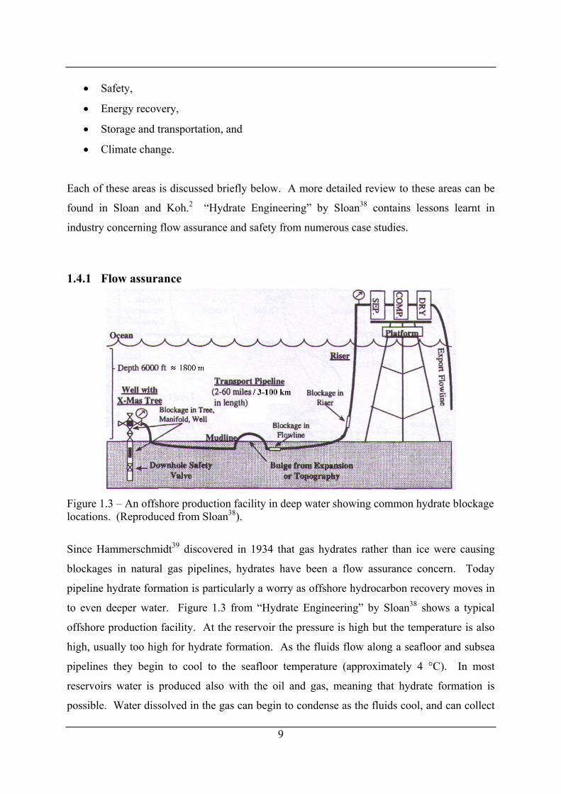
Figure 1.3 – An offshore production facility in deep water showing common hydrate blockage
locations. (Reproduced from Sloan38). .......................................................................... 9
Figure 1.4 – Current radial dissociation picture (a), compared to the old axial dissociation
picture (b). (Adapted from Sloan2).............................................................................. 12
Figure 1.5 – Structure of tetra-n-butylammonium ·38H2O around the cation showing alkyl
chain occupation of larger cages (2×51262 – tetrakaidecahedrons and 2×51263 –
pentakaidecahedrons), cation centre replacement of water lattice site and small 512
cages that could be occupied with suitably sized molecules (represented by spheres).
(Reproduced from Shimada et al.62)............................................................................. 14
Figure 1.6 – Temperature-mass fraction (T,w) stability diagram for tetraisopentylammonium
fluoride (1) + water (2) at atmospheric pressure, composition of semi-clathrate
hydrates are represented by the ratios of moles of salt to moles of water, 1:38, 1:32.8
and 1:27. (Reproduced from plotted data of Lipkowski et al.67)................................. 16
Figure 1.7 – Cages of semi-clathrate hydrate structures; Note: cages not to scale. Cages were
produced in ACD Chemsketch 10.70 ............................................................................ 19
Figure 2.1 – Differential thermal analysis schematic; s = sample, r = reference, h = heat
source, Ts = sample temperature, Tr = reference temperature, ΔT = differential
thermocouple. ............................................................................................................... 25
Figure 2.2 – Boersma’s original sample holder design); s = sample, r = reference, h = heat
source, tc = differential thermocouple. (Reproduced from Mraw77)........................... 25
Figure 2.3 – Electrical circuit equivalent of heat flux DSC; E = temperature of the furnace, Rs
= thermal resistance between the furnace and sample, Rr = thermal resistance between
the furnace and reference crucible, Us = temperature of the sample, Ur = temperature
of the reference, Cs = heat capacity of the sample and crucible, and Cr = heat capacity
of the reference and crucible. (Reproduced from Claudy75 in Goodwin et al.74)........ 27
Figure 2.4 – Electrical circuit equivalent of heat flux DSC with coupled cells; E = temperature
of the furnace, Rs = thermal resistance between the furnace and sample crucible, Rr =
thermal resistance between the furnace and reference crucible, Rcc = thermal resistance
between the sample and reference crucibles, Us = temperature of the sample, Ur =
temperature of the reference, Φ = heat flux emanating from the sample, Cs = heat
capacity of the sample, Cdk = heat capacity of the disk, = heat capacity of the
sample crucible, = heat capacity of the reference crucible, and Cr = heat capacity
of the reference material. (Reproduced from Claudy75 in Goodwin et al.74). ............. 28
scrC
rcrC
Figure 2.5 – DSC recorded thermal transition peak of differential power (ΔP) versus
monitored sample temperature (Tsm); Ttr = extrapolated onset temperature of transition.
...................................................................................................................................... 31
Figure 2.6 – Calscorp MC-DSC 4100 HT DSC measuring unit; RTD = Resistance
temperature detector, T.E.D = Thermoelectric device. (Reproduced from user’s
manual79). ..................................................................................................................... 31
Figure 2.7 – Reflection of X-rays from successive layers of atoms in a crystal. (a) The
reflected waves are exactly in phase a reinforce each other. (b) the reflected waves are
out of phase and cancel out, d = interatomic spacing, θ = incident angle of X-ray.
(Modified from Jones and Childers89).......................................................................... 33
xii
xiii
Figure 2.8 – Illustration of diffraction paths difference, maxima occur at angle where 2dsinθ
is an integer multiple of wavelengths. (Reproduced from Jones and Childers89). ...... 34
Figure 2.9 – X-ray diffractogram for hexagonal ice, sI hydrate and sII hydrate; d-values in
Ångströms are listed above the peaks, data generated using PowderCell87 using the
data of Owston88 for hexagonal ice and Kirchner et al.26 for sI hydrate (methane
hydrate) and sII hydrate (methane + ethanol + propane), λ = 0.70903165 Å. ............. 34
Figure 2.10 – An example of X-ray diffraction instrumentation. ............................................ 35
Figure 2.11 – Light encountering a molecule by Rayleigh and Raman scattering; ν =
frequency of photon/ray of light, Δν = difference between scattered light frequency
and incident light frequency, h = Planck’s constant, ΔElight = difference in energy
between the incident and scattered photon, ΔEmolecule = - ΔElight = energy gained by
molecule during scattering process. ............................................................................. 36
Figure 2.12 – Energy level diagram for Raman and Rayleigh Scattering. (Adapted from
Skoog et al.90). .............................................................................................................. 38
Figure 2.13 – The electromagnetic wave. (Adapted from Skoog et al.90)............................... 38
Figure 2.14 – Fibre optic sample illumination system; (a) Schematic of system, (b) Probe
showing fibre bundle containing input and collection fibres (c) Collection fibre
linearly arranged to enter monochromator slot. (Reproduced from Skoog et al.90).... 41
Figure 2.15 – Raman spectra in the C-H region for hydrates formed from methane + ethane
gas mixtures showing the slight differences in Raman shifts for enclathrated molecules
in sI and sII hydrates. (Reproduced from Subramanian et al.72). ................................ 42
Figure 2.16 – TCD detector, an arrangement of two sample detector and two reference
detector cells. (Reproduced from Skoog et al.90). ....................................................... 45
Figure 2.17 – Schematic of a gas chromatograph with a thermal conductivity detector. ........ 45
Figure 2.18 – Chromatogram showing the retention times and the extrapolated base widths of
two components............................................................................................................ 46
xiv
Figure 2.19 – NMR energy levels for a hydrogen nuclei (proton)........................................... 51
Figure 2.20 - Precession of a spinning nucleus in a magnetic field showing the absorption of a
photon at the frequency of precession and the association nuclear spin flip. (Adapted
from Brown103). ............................................................................................................ 52
Figure 2.21 – Basic components of NMR spectrometers. (Adapted from Brown103)............. 53
Figure 2.22 – NMR spectra of the tetrahexylammonium ion in DMSO-d6. (Modified from
Sigma Aldrich online catalog109).................................................................................. 56
Figure 2.23 – NMR spectra of trihexylamine in CDCl3. (Modified from Sigma Aldrich online
catalog107). .................................................................................................................... 56
Figure 3.1 – Isothermal (T = 277.6 K) pressure versus composition phase diagram of
methane (1) + ethane (2) + excess water; generated using a van der Waals and
Platteeuw based statistical model, x1 is the water free mole fraction of methane, phase
labels: Lw = liquid water, V = vapour, sI = structure I hydrate, sII = structure II
hydrate, experimental points are from Deaton and Frost.120 (Modified from
Subramanian et al.71). ................................................................................................... 60
Figure 3.2 – Size-structure classification of single guest component and binary guest
component hydrates; potential guest molecules are divided into size ranges a, b and c
(i.e. for sII a = occupies 512 cages, b = mostly occupies 51264 cages and c = too large to
occupy either cage). The following combinations are known, although some of the
boundaries may not have been firmly established: Ia + Ib →structures I or II; IIa or Ia
+ IIb → structure II; Ia or IIa +IIc → structure II; and Ia or IIa +Hc → structure H.
(Modified from Ripmeester119). ................................................................................... 61
Figure 3.3 – Kihara collision radius (σ) guest size ranges for a mixture of “small” and “large”
pseudo-methane molecules showing predicted sII double guest hydrate transitions;, the
region of “sI or sII” indicate that at some composition of the mixture “small guest” +
“large guest” sII hydrates will form, for the “sI only” region only sI hydrates were
predicted for all mixture compositions. (Modified from Hester121)............................ 62
xv
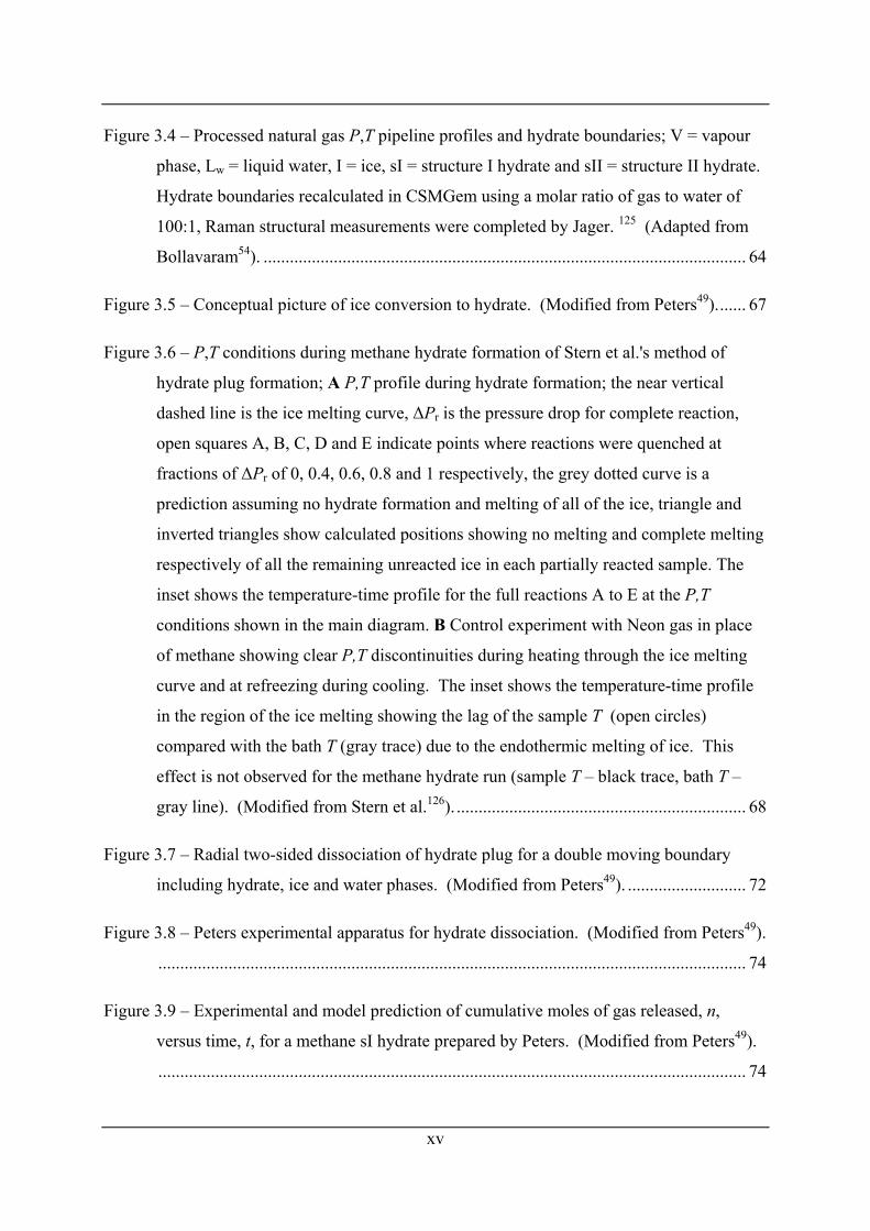
Figure 3.4 – Processed natural gas P,T pipeline profiles and hydrate boundaries; V = vapour
phase, Lw = liquid water, I = ice, sI = structure I hydrate and sII = structure II hydrate.
Hydrate boundaries recalculated in CSMGem using a molar ratio of gas to water of
100:1, Raman structural measurements were completed by Jager. 125 (Adapted from
Bollavaram54). .............................................................................................................. 64
Figure 3.5 – Conceptual picture of ice conversion to hydrate. (Modified from Peters49)....... 67
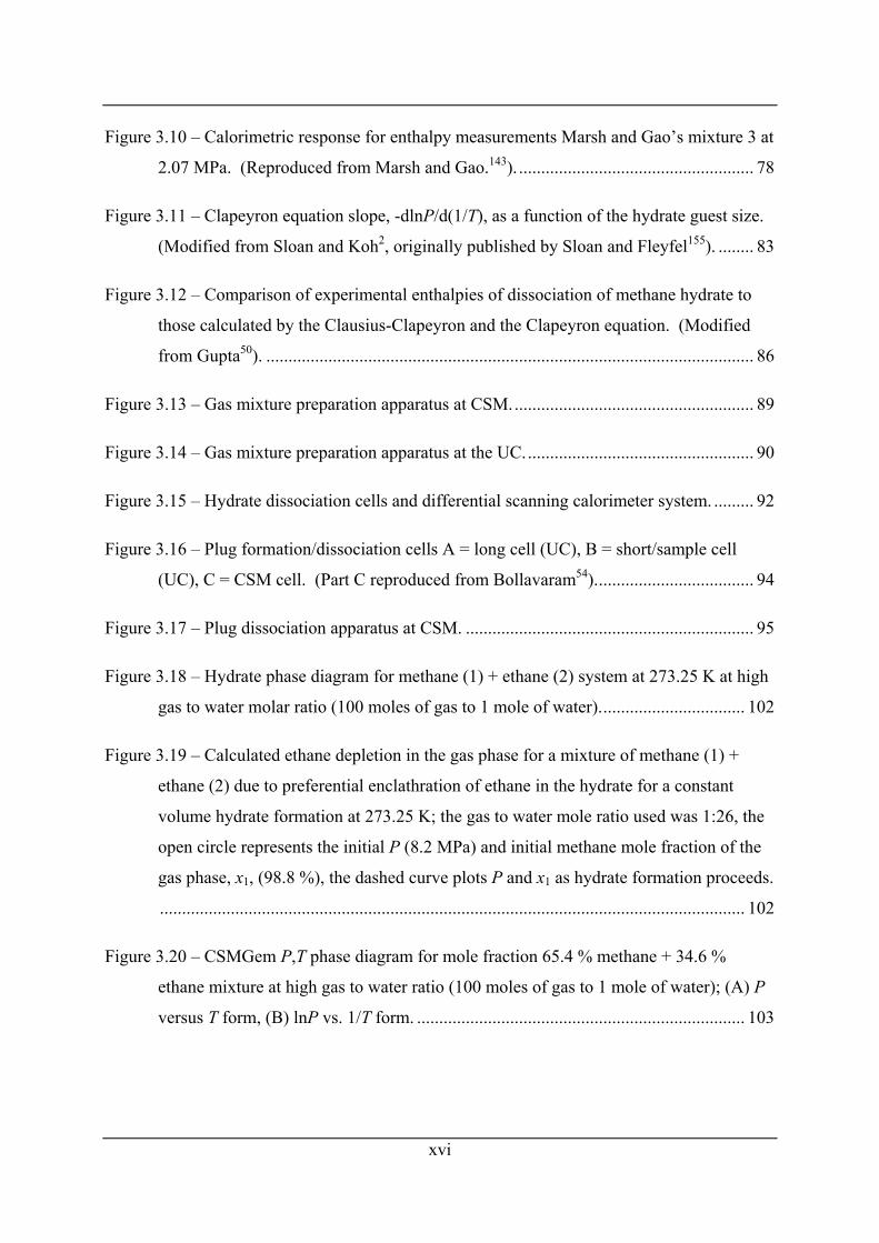
Figure 3.6 – P,T conditions during methane hydrate formation of Stern et al.'s method of
hydrate plug formation; A P,T profile during hydrate formation; the near vertical
dashed line is the ice melting curve, ΔPr is the pressure drop for complete reaction,
open squares A, B, C, D and E indicate points where reactions were quenched at
fractions of ΔPr of 0, 0.4, 0.6, 0.8 and 1 respectively, the grey dotted curve is a
prediction assuming no hydrate formation and melting of all of the ice, triangle and
inverted triangles show calculated positions showing no melting and complete melting
respectively of all the remaining unreacted ice in each partially reacted sample. The
inset shows the temperature-time profile for the full reactions A to E at the P,T
conditions shown in the main diagram. B Control experiment with Neon gas in place
of methane showing clear P,T discontinuities during heating through the ice melting
curve and at refreezing during cooling. The inset shows the temperature-time profile
in the region of the ice melting showing the lag of the sample T (open circles)
compared with the bath T (gray trace) due to the endothermic melting of ice. This
effect is not observed for the methane hydrate run (sample T – black trace, bath T –
gray line). (Modified from Stern et al.126). .................................................................. 68
Figure 3.7 – Radial two-sided dissociation of hydrate plug for a double moving boundary
including hydrate, ice and water phases. (Modified from Peters49). ........................... 72
Figure 3.8 – Peters experimental apparatus for hydrate dissociation. (Modified from Peters49).
...................................................................................................................................... 74
Figure 3.9 – Experimental and model prediction of cumulative moles of gas released, n,
versus time, t, for a methane sI hydrate prepared by Peters. (Modified from Peters49).
...................................................................................................................................... 74
xvi
Figure 3.10 – Calorimetric response for enthalpy measurements Marsh and Gao’s mixture 3 at
2.07 MPa. (Reproduced from Marsh and Gao.143). ..................................................... 78
Figure 3.11 – Clapeyron equation slope, -dlnP/d(1/T), as a function of the hydrate guest size.
(Modified from Sloan and Koh2, originally published by Sloan and Fleyfel155). ........ 83
Figure 3.12 – Comparison of experimental enthalpies of dissociation of methane hydrate to
those calculated by the Clausius-Clapeyron and the Clapeyron equation. (Modified
from Gupta50). .............................................................................................................. 86
Figure 3.13 – Gas mixture preparation apparatus at CSM....................................................... 89
Figure 3.14 – Gas mixture preparation apparatus at the UC.................................................... 90
Figure 3.15 – Hydrate dissociation cells and differential scanning calorimeter system. ......... 92
Figure 3.16 – Plug formation/dissociation cells A = long cell (UC), B = short/sample cell
(UC), C = CSM cell. (Part C reproduced from Bollavaram54).................................... 94
Figure 3.17 – Plug dissociation apparatus at CSM. ................................................................. 95
Figure 3.18 – Hydrate phase diagram for methane (1) + ethane (2) system at 273.25 K at high
gas to water molar ratio (100 moles of gas to 1 mole of water)................................. 102
Figure 3.19 – Calculated ethane depletion in the gas phase for a mixture of methane (1) +
ethane (2) due to preferential enclathration of ethane in the hydrate for a constant
volume hydrate formation at 273.25 K; the gas to water mole ratio used was 1:26, the
open circle represents the initial P (8.2 MPa) and initial methane mole fraction of the
gas phase, x1, (98.8 %), the dashed curve plots P and x1 as hydrate formation proceeds.
.................................................................................................................................... 102
Figure 3.20 – CSMGem P,T phase diagram for mole fraction 65.4 % methane + 34.6 %
ethane mixture at high gas to water ratio (100 moles of gas to 1 mole of water); (A) P
versus T form, (B) lnP vs. 1/T form. .......................................................................... 103
xvii
Figure 3.21 – CSMGem P,T phase diagram for mole fraction 98.8 % methane + 1.2 % ethane
mixture at high gas to water ratio (100 moles of gas to 1 mole of water); (A) P versus
T form, (B) lnP vs. 1/T form. ..................................................................................... 104
Figure 3.22 – Hydrate plug dissociation plot of mole of gas released, n, as a function of time,
t, for sI hydrate plug prepared from the mixture with mole fractions of 65.4 % methane
+ 34.6 % ethane.......................................................................................................... 106
Figure 3.23 – Hydrate plug dissociation plot of mole of gas released, n, as a function of time,
t, for sII hydrate plug prepared from the mixture with mole fractions of 65.4 %
methane + 34.6 % ethane. .......................................................................................... 106
Figure 3.24 – CSMGem predicted P,x phase diagram at 273.25 K for methane (1) + ethane (2)
mixtures for x1 = (0.55 to 0.8) and a high gas to water mole ratio (100:1) showing the
experimental formation P and predicted x1 for the formation of a sII hydrate from a
65.4 % methane + 34.6 % ethane mole fraction gas mixture; the break in the P,x1
tracking line signifies a repressurization. ................................................................... 107
Figure 3.25 – Experimental and predicted hydrate dissociation times, tD, versus hydrate plug
porosity, ε, for plugs prepared and dissociated at the University of Canterbury. ...... 108
Figure 3.26 – Raman spectra of sII hydrate prepared from 65.4 % methane + 34.6 % ethane
mole fraction mixture above 10 MPa (the formation conditions of this hydrate are
shown in Figure 3.24)................................................................................................. 109
Figure 3.27 – Example X-ray diffraction rings indexing to a sII hydrate; refer to the predicted
powder pattern in Chapter 2. ...................................................................................... 109
Figure 3.28 – Hydrate dissociation for plug prepared from the 98.8 % methane + 1.2 % ethane
mole fraction mixture showing evidence of mixed sI and sII hydrate plug with a sII
dominated dissociation time....................................................................................... 110
Figure 3.29 – Calorimetry power, P, versus temperature scan for the dissociation of a sII
hydrate formed in the short sample cell and dissociated in the 98.8 % methane + 1.2 %
ethane gas mixture at 6.92 MPa; note: baselines have been deducted from these peaks.
.................................................................................................................................... 111
xviii
Figure 3.30 – Clapeyron equation enthalpies of dissociation predicted from CSMGem phase
data for the mixture of mole fraction 65.4 % methane + 34.6 % ethane sI and sII
hydrates, the mixture of mole fraction 98.8 % methane + 1.2 % ethane sII hydrates and
methane sI hydrate. Experimental measurements are shown for comparison. ......... 112
Figure 3.31 – Average guest size, Dave, calculated from CSMGEM fractional cage occupancy
and molecular diameters of methane and ethane as a function of pressure for sI hydrate
prepared from 65.4 % Me + 34.6 % Et mixture (for a mole ratio of gas to water of
100)............................................................................................................................. 114
Figure 3.32 – Average guest size, Dave, calculated from CSMGEM fractional cage occupancy
and molecular diameters of methane and ethane as a function of pressure for sII
hydrate prepared from 65.4 % Me + 34.6 % Et mixture (for a mole ratio of gas to
water of 100). ............................................................................................................. 114
Figure 4.1 – Mole fraction in the hydrate phase on a water free basis of methane, xCH4, as a
function of the vapour phase mole fraction of methane, yCH4, used to prepare hydrates
from methane + ethane mixtures, compositions were calculated from NMR peak areas
or estimated from Raman spectra peaks areas, abrupt changes in the range 0.686-0.784
indicate the stable hydrate structure changes from sI to sII, a similar effect is seen near
yCH4 =1. (Modified from Subramanian et al.71). ........................................................ 132
Figure 4.2 – Constant pressure syringe or piston pump formation of hydrate from ice particles.
.................................................................................................................................... 135
Figure 4.3 – Algorithm for gas phase stripping and preferential enclathration for a constant
pressure syringe or piston pump formation of gas hydrate for a gas mixture. Note:
Initial conditions (described by eqs (4.3) through to (4.9)) have to be prior calculated
to use this algorithm. .................................................................................................. 141
Figure 4.4 – Constant volume system for formation of hydrate from ice particles. .............. 142
Figure 4.5 – Algorithm for the gas phase stripping and preferential enclathration for a constant
volume formation of gas hydrate for a gas mixture. Note: Initial conditions (described
by eqs (4.25) through to(4.30)) have to be prior calculated to use this algorithm. .... 148
xix
Figure 4.6 – Experimental apparatus for preferential enclathration formation tests at constant
P (maintained by ISCO syringe pump). PRT refers to platinum resistance
thermometers (not to scale). ....................................................................................... 152
Figure 4.7 – Syringe used to gas samples showing alternative positions of the 3-way stopcock.
.................................................................................................................................... 154
Figure 4.8 – Volume of the ISCO syringe pump and temperature of the cell as a function of
time............................................................................................................................. 159
Figure 4.9 – Comparison of experimental and model preferential enclathration stripping of the
gas phase. ................................................................................................................... 160
Figure 4.10 – Laboratory experimental set-up for hydrate formation from melting ice particles
to avoid gas phase composition changes by the use of two gas supplies................... 164
Figure 5.1 – P,T SCH + Aq + V phase measurements for the system hydrogen + TBAB
aqueous solution at mole fraction of TBAB, x, in the solution. (Modified from
Hashimoto et al.47)...................................................................................................... 169
Figure 5.2 – Dissociation point determination from pre-dissociation point P,T measurements
and post-dissociation point P,T measurements. (Modified from Tohidi et al.170). ... 172
Figure 5.3 – Measurements of dissociation conditions of H2+ TBAB SCH and H2 + TBAF
SCH, also plotted are data for pure H2 sII hydrate and H2 + THF sII hydrate. a H2 sII
hydrate data from Mao et al.171 b H2 + THF sII hydrate data from Florusse et al.31
(Modified from Chapoy et al.45)................................................................................. 172
Figure 5.4 – T, w phase diagram for TBAB + water under atmospheric conditions, numbers
along the vertical lines refer to hydration numbers. (Modified from Arjmandi et al.44
data from Lipkowski et al.172, Oyama et al.69 Darbouret et al.173). ........................... 173
Figure 5.5 – Methane + TBAB + water phase boundaries, w = mass fraction of TBAB in
solution. (Modified from Arjmandi et al.44, note: methane hydrate line was calculated
by Arjmandi et al. using the Heriot Watt Hydrate (HWHYD) model.174,175). ........... 173
xx
Figure 5.6 – Bulk mass fraction of hydrogen, wH2, stored as a function of the TBAB mole
fraction, xTBAB, in the solution used to prepare the SCH. (Modified from Strobel et
al.176)........................................................................................................................... 175
Figure 5.7 - Volume fraction of natural gas in SCH of TBAB. (Modified from Ahmadloo et
al.177). (w = mass fraction of salt in aqueous solution).............................................. 177
Figure 5.8 - Approximated capital cost of 4×10⁹ m3 STP per year of natural gas with distance
transported. NGH = Natural gas hydrate. (Modified from Gudmundsson et al.183) 179
Figure 5.9 – Floating production, storage and offloading (FPSO) associated gas NGH slurry
transport cost as a function of distance. (Modified from Gudmundsson et al.183) ..... 179
Figure 5.10 - Capacity-distance diagram for natural gas transport. (Modified from
Gudmundsson et al.183). LNG = liquified natural gas, CNG = compressed natural gas,
GTW = gas to wire, NGH = natural gas hydrate, GTL = gas to liquids. ................... 180
Figure 5.11 – Reflux apparatus for the preparation of tetraisopentylammonium bromide.... 185
Figure 5.12 – Proton NMR spectrum of TIPAF in CD3OD; TIPAF hydrogen peaks are
labelled 1, 2, 3 or 4 with respect to the hydrogen of the molecule drawn, numerical
values below the axis indicate relative peak areas, inset shows one sample peak and
two peaks that were also present in a solvent only spectrum. Note: methanol and water
peaks at higher chemical shift are not shown............................................................. 186
Figure 5.13 – Apparatus for P,T tetraisopentylammonium fluoride solution + methane semi-
clathrate hydrate phase equilibria measurements....................................................... 189
Figure 5.14 – Example of the equilibrium steps to determine a tetraisopentylammonium
fluoride aqueous solution (TIPAF·38.3H2O) + methane P,T SCH + Aq + V point... 193
Figure 5.15 – P,T SCH + Aq + V equilibria points for TIPAF (w = 0.315) + methane
compared to TBAB (w = 0.3) + methane from Arjmandi et al.44 and methane hydrate
data calculated using CSMGem the atmospheric melting point of each SCH is also
shown (for TIPAF from Lipkowski et al.67, for TBAB estimated from Figure 5.4).. 194
xxi
Figure A.1 – The fourteen Bravais lattices groups according to the seven crystal systems.
(Reproduced from Huheey et al.196). .......................................................................... 222
Figure E.1 – Density – temperature phase diagram for ethane calculated using NIST
REFPROP.168.............................................................................................................. 230
Figure E.2 – Phase diagram for methane (1) + ethane (2) mixture at 20 °C where x2 is the
mole fraction of ethane, calculated using NIST REFPROP.168.................................. 230
Figure G.1 – Pressure testing of the cells. (a) Apparatus diagram. (b) Photograph with long
cell in place................................................................................................................. 233
xxii
LIST OF TABLES
Table 1.1 – Approximate cage sizes for structure I and structure II hydrates............................ 4
Table 1.2 – Tetraisopentylammonium fluoride semi-clathrate hydrates: stoichiometry,
crystallographic details, cage structures and densities. ................................................ 17
Table 1.3 – Potential occupancies for gas storage of methane in semi-clathrate hydrate
structures. ..................................................................................................................... 18
Table 2.1 – Chemical shifts of hydrogen nuclei important for tertiary amine and quaternary
ammonium salt analysis. .............................................................................................. 55
Table 2.2 – 1H NMR resonances of tetraisopentylammonium iodide in D2O. (Reproduced
from Harmon et al.104). ................................................................................................. 55
Table 3.1 – Processed natural gas composition. (Reproduced from Bollavaram54). .............. 65
Table 3.2 – Calorimetric measurements of enthalpies of dissociation for single guest hydrates
of natural gas components............................................................................................ 79
Table 3.3 – Comparison of the Clausius-Clapeyron calculated and experimental above ice
point enthalpies of dissociation at 273.15 K. ............................................................... 83
Table 3.4 – Methane + Ethane gas mixture mole fractions and purities. ................................. 89
Table 3.5 – Calorimetry Sciences Corporation MC-DSC 4100 Uncertainties, setabilites and
stabilities....................................................................................................................... 98
Table 3.6 – Hydrate dissociations of plugs formed to investigate high methane composition
structural transition..................................................................................................... 108
Table 3.7 – Enthalpy of hydrate dissociation for sII hydrate prepared from 98.8 % Me + 1.2 %
Et gas mixture............................................................................................................. 112
Table 3.8 – Calculated dissociation enthalpies from CSMGem data for 65 % methane + 35 %
ethane and 98.8 % methane + 1.2 % ethane mixtures at atmospheric pressure. ....... 113
xxiii
Table 4.1 – Mole fractions of each component in Hammerschmidt’s pipeline gas and hydrate
gas. (Reproduced from Hammerschmidt39). ............................................................. 130
Table 5.1 – Mole fractions of the components in the natural gas used by Ahmadloo et al.177
.................................................................................................................................... 177
Table 5.2 - Estimated methane mass fraction, mass density and dissociation temperature of
several hydrates and LNG.......................................................................................... 181
Table 5.3 – Chemical purities for preparation and purification of TIPAF............................. 184
Table 5.4 – Proton NMR chemical shifts and calculated hydrogen atoms for each shift/peak
.................................................................................................................................... 187
Table 5.5 – Specifications of experimental equipment for P,T phase measurements............ 191
Table 5.6 – P,T SCH + Aq + V equilibria points for TIPAF (w = 0.315) + methane............ 194
Table A.1 – The seven crystal systems. (Modified from Wells197)....................................... 221
Table A.2 – Hermann-Manguin space group symbolism. (Modified from Ferraro et al.198).
.................................................................................................................................... 223
Table B.1 – Generated atoms making up a 5444 cage. ........................................................... 225
Table B.2 – Comparison of sphericity of cages. .................................................................... 225
Table C.1 – Electrical equivalents of thermal properties for the electrical circuit analogy.
(Adapted from Claudy75)............................................................................................ 226
Table I.1 – Estimations of volumes of the cell and constant volume system (between valve A
and relief valve of Figure 5.13). ................................................................................. 236
1
Chapter 1 INTRODUCTION
1.1 What are clathrate hydrates? Clathrates are crystalline inclusion compounds in which one group of molecules form a lattice
of cages in which other so called “guest” molecules are encaged or enclathrated. Clathrate
hydrates are clathrates in which the lattice is constructed from hydrogen bonded water
molecules. For a clathrate hydrate to be stable it is essential that guest molecules occupy at
least some of the cages. Although strictly speaking clathrate hydrates are non-stoichiometric
the near full occupation (90 % or greater) of at least one type or size of cages in the structure
is required for stability. Clathrate hydrate formation is favoured by low temperature and high
pressure conditions. Clathrate hydrates may be formed from water and gaseous guests such as
methane and carbon dioxide or water and liquid guests such as tetrahydrofuran and
cyclopentane. Natural gas hydrates refer to clathrate hydrates in which the guest molecules
consist of constituents of natural gas.1,2
Semi-clathrate hydrates (SCH)3,4 are clathrates in which water forms a lattice with the help of
quaternary ammonium (R4N+), quaternary phosphonium (R4P+), or tertiary sulfonium (R3S+)
salts, collectively termed peralkylonium salts, or trialkylamine or trialkylphosphine oxides. In
the case of the peralkylonium salts the nitrogen, phosphorus or sulfur atoms as well as the
anion (which might commonly be a halide) occupy lattice sites in the structure. In the case of
the trialkyl(amine/phosphine) oxide the nitrogen/phosphorus atoms and oxygen atoms occupy
lattice sites. The alkyl chains of the SCH former act as guests in some of the cages.5 The
most stable of these SCH form with cations containing the n-butyl or isopentyl alkyl chains.6
For the peralkylonium salt SCH anions of a similar size to the water molecule such as the
fluoride ion tend to result in more stable hydrate phases.7,8 SCH are stable at atmospheric
pressure at temperatures as high as the mid 30 °Cs.3
1.2 Structure and stoichiometry of clathrate hydrates
1.2.1 Structure of gas clathrate hydrates The first documented observation of what would now be recognized as a clathrate hydrate
was by Joseph Priestly in 1778.9 Priestly had cooled an aqueous solution of sulfur dioxide to
2
approximately -8 °C and he noted “as it melted the ice sank to the bottom of the liquor”, what
he was in fact observing was sulfur dioxide hydrate (density = 1300 kg·m-3,10 dissociation
temperature at atmospheric pressure = 6.8 °C 11). Humphry Davy later observed in 1811 that
“the solution of [chlorine] in water freezes more readily than pure water”.12 A more definitive
discovery of clathrate hydrates was made by Michael Faraday under the supervision of Davy
in 1823.13 He studied the solid formed in an aqueous chlorine solution and determined its
composition to be Cl2·10H2O. The most pertinent observation made by these early hydrate
scientists was the ice-like appearance of clathrate hydrates. Since Faraday’s work a wide
range of gases of small molecular volume have been observed to form clathrate hydrates,
including simple hydrocarbons and noble gases. Clathrate hydrates of liquids with small
molecular volumes such as chloroform, tetrahydrofuran and acetone have also been reported.
Sloan and Koh2 tabulate an extensive list of hydrate formers in table 2.5a of their book.
In the early 1940’s von Stackelberg and co-workers began X-ray studies of clathrate
hydrates.14 Two unique cubic crystal structures were identified from single crystals, one with
a unit cell size of 12 Å and space group of Pm3n from the analysis of a sulfur dioxide hydrate
and the other structure “that would appear to have space group [P4232]”15 from the analysis of
a chloroform and hydrogen sulfide double hydrate (see Appendix A for a brief description of
crystal systems and space groups). The data from these analyses was lost during World War
II and could not be further investigated, nevertheless a hydrogen bonded structure was
proposed by von Stackelburg16 that included voids that could hold gas molecules. This
structure however was deemed to be physically unrealistic due to low O-H··O bond distances
[(2.42 to 2.6) Å versus 2.76 Å in hexagonal ice] and O-O-O bond angles that deviated greatly
from the tetrahedral angle [(61 to 145)° versus the tetrahedral 109.5°]. Claussen17,18
considered a hydrogen bonded pentagonal dodecahedral as a starting point for considering
hydrate structures because the 108° bond angles differed little from the tetrahedral 109.5°. He
constructed a cubic cell consisting of 136 water molecules formed from 16 pentagonal
dodecahedrals cages, referred to in short hand as 512 cages (where the 5 refers to the
pentagonal shape of each face and 12 refers to the number of faces of that shape in the cage),
and 8 slightly larger hexakaidecahedrons or 51264 cages consisting of 12 pentagonal faces and
4 hexagonal faces. This structure was confirmed by von Stackelberg and Müller19,20 for
hydrates they had prepared from larger molecules such as chloroform and ethyl chloride and
3
their double hydrates with hydrogen sulfide. The space group was confirmed as Fd3m, rather
than the originally supposed P4232, with a unit cell size of 17.2 Å. The other structure with a
unit cell size of 12 Å was soon also solved almost simultaneously by Claussen21, Müller and
von Stackelberg22, and Pauling and Marsh.23 This structure has a unit cell of 46 water
molecules composed of two pentagonal dodecahedral cages (512 cages) and six
tetrakaidecahedral or 51262 cages consisting of 12 pentagonal faces and 2 hexagonal faces.
These two structures are designated structure I (sI) for the (2×512 cage + 6×51262 cage)·46H2O
and 12 Å unit cell hydrate and structure II (sII) for the (16×512 cage + 8×51264 cage)·136H2O
and 17 Å unit cell hydrate. These two structures are the most common gas hydrate structures
encountered and are shown in Figure 1.1, approximate cage sizes for these structures are
shown in Table 1.1. Detailed X-ray studies of the two structures were published in 1965 by
McMullan and Jeffrey24 (sI – ethylene oxide hydrate) and Mak and McMullan25 (sII –
tetrahydrofuran and hydrogen sulphide double hydrate). In 2004 Kirchner et al.26 published
detailed single crystal X-ray analyses for methane sI, propane sII, and several other hydrates.
Structure H (sH) hydrates are also shown in Figure 1.1 however these hydrate require a larger
approximately spherical molecule such as neohexane as well as a smaller molecule such as
methane to be stable and are not encountered in this work.
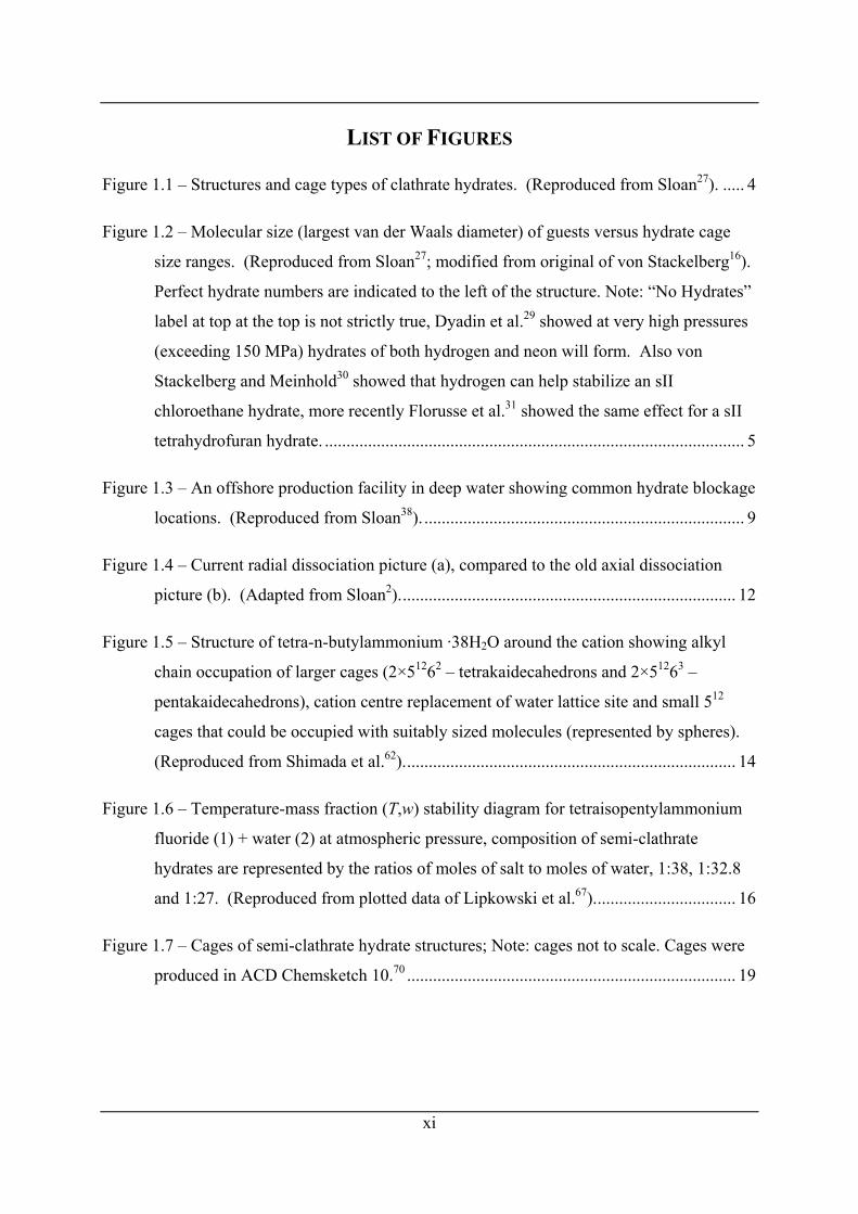
1.2.2 Occupation of cage by guest molecules and stoichiometry of hydrates Figure 1.2 from Sloan27 (modified from von Stackelberg16) plots the size of various molecules
(mainly natural gas constituents) in terms of their largest van der Waals diameter and labels
the structure of hydrates that they form (sI or sII) Table 1.1 includes approximate sizes of the
cages that make up sI and sII hydrates. From Figure 1.2 it can been seen that small molecules
less than 4.5 Å form sII hydrates by occupancy of the both the small 512 cage and large 51264
cage, molecules sized between (4.5 and 5.1) Å form sI hydrates with occupancy of both cages
(512 and 51262), molecules sized between (5.1 and 5.8) Å form sI hydrates with occupancy of
only the large 51262 cage and molecules sized between (5.8 and 7.0) Å form sII hydrates with
occupancy of the large 51264 cages only. Molecules greater than 7.0 Å are too large to fit in
the cages of sI or sII hydrates although they may form sH with the help of a molecule smaller
than 5.2 Å.
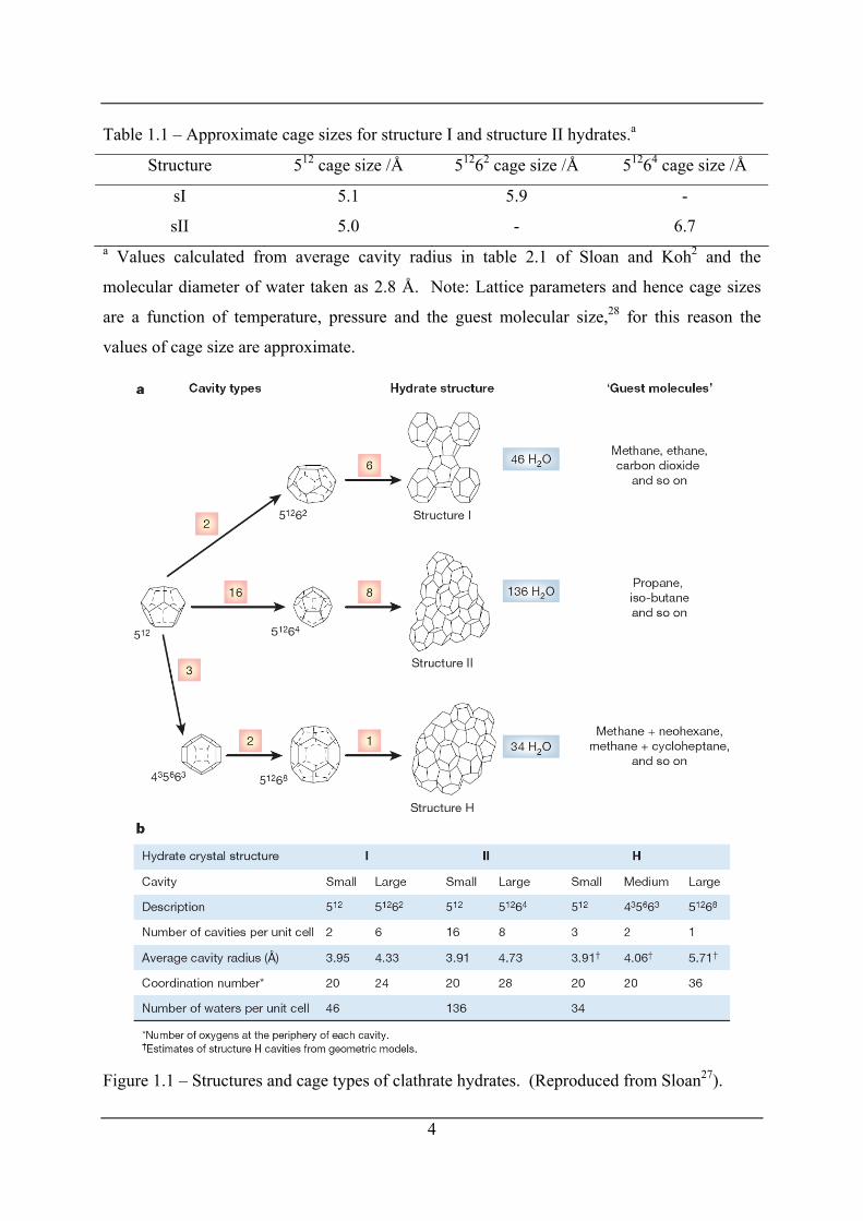
Table 1.1 – Approximate cage sizes for structure I and structure II hydrates.a
Structure 512 cage size /Å 51262 cage size /Å 51264 cage size /Å
sI 5.1 5.9 -
sII 5.0 - 6.7 a Values calculated from average cavity radius in table 2.1 of Sloan and Koh2 and the
molecular diameter of water taken as 2.8 Å. Note: Lattice parameters and hence cage sizes
are a function of temperature, pressure and the guest molecular size,28 for this reason the
values of cage size are approximate.
Figure 1.1 – Structures and cage types of clathrate hydrates. (Reproduced from Sloan27).
4
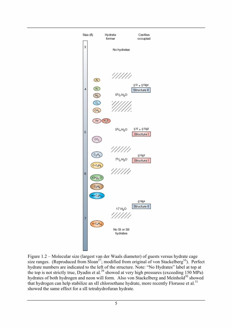
Figure 1.2 – Molecular size (largest van der Waals diameter) of guests versus hydrate cage size ranges. (Reproduced from Sloan27; modified from original of von Stackelberg16). Perfect hydrate numbers are indicated to the left of the structure. Note: “No Hydrates” label at top at the top is not strictly true, Dyadin et al.29 showed at very high pressures (exceeding 150 MPa) hydrates of both hydrogen and neon will form. Also von Stackelberg and Meinhold30 showed that hydrogen can help stabilize an sII chloroethane hydrate, more recently Florusse et al.31 showed the same effect for a sII tetrahydrofuran hydrate.
5
1.3 Clathrate hydrate thermodynamic prediction models
1.3.1 The van der Waals and Platteeuw model Experimentally it is has been shown that clathrate hydrates are non-stoichiometric, sI methane
hydrate for example typically has a hydrate number of about 6 versus the perfect
stoichiometric value of 5.75 which would result from full occupation of all cages (46 water
molecules divided by 8 cages). Sloan and Koh2 note that “typical occupancies of large
cavities are greater than 95 %, while occupancy of small cavities vary widely depending on
the guest composition, temperature and pressure”. The statistical thermodynamic model of
clathrates developed by van der Waals and Platteeuw32 (also described in detail in Chapter 5
of Sloan and Koh2 and in Ballard33) takes in to account this non-stoichiometry of clathrate
hydrates (note: this model is generalized for all clathrate formers however for the purposes of
this discussion reference will only be made to clathrate hydrates). The water of the hydrate is
considered to be effectively a “solvent” and the guest molecules are considered to be
“solutes” allowing for non-occupation of some cages. Details of the derivation of this model
will not be considered in detail here however the assumptions upon which the model is based
include:
• The guest molecules do not significantly distort the cages, so that the vibrational and
electronic modes of the hydrogen bonded hydrate host network are not effected,
• Cages are only occupied by one guest molecule,
• The interactions between enclathrated guest molecules are negligible so that the
partition function for the guest molecules is independent of the number and types of
guest molecules present,
• Classical statistics are valid (quantum effects do not need to be considered).
The net result of the model is an equation which describes the chemical potential of water in
the hydrate lattice, HWμ :
, (1.1) H βW W ,
J
ln 1 θii
kTμ μ ν ⎛= + −⎜⎝ ⎠
∑ ∑ J i⎞⎟
6
where βWμ is the chemical potential of a theoretical empty hydrate lattice, k is Boltzmann’s
constant, T is the absolute temperature, i is the type of cavity (e.g. a 512 cage), νi is the
number of type i cavities per water molecule, J is the type of guest molecule and θJ,i is the
fractional occupancy of cavity type i by molecule of type J. The fractional occupancy, θJ,i is
given by the Langmuir isotherm:
,J,i
,
θ1
J i J
J i JJ
C fC f
=+∑
, (1.2)
where CJ,i is a Langmuir adsorption constant for the molecule of type J in cavity of type i and
fJ is the fugacity of a molecule of type J. It is possible to show (see Sloan and Koh2 section
5.1.4) that the Langmuir adsorption constant CJ,i may be calculated using eq (1.3) if it is
assumed that:
• Enclathration does not effect the rotational, vibrational, nuclear or electronic energies,
and
• The potential energy of a guest molecule is only a function of its distance from the
cavity centre. This means that the cavity in effect is spherically averaged and a
symmetric potential function, ( )rϖ , can be used, were r is the distance from the
centre of the cage.
( )R 2
, 0
4π exp dJ iC rkT
ϖ= −⎡ ⎤⎣ ⎦∫ kT r r (1.3)
The upper integral limit of eq (1.3), R, represents the free cavity radius (which is the average
cavity radius minus the radius of the water molecule). A Kihara potential is typically used to
generate the spherically symmetric potential function. The pair potentials are averaged
between the guest molecule and each water molecules of the cage. Kihara parameters are
fitted to the hydrate formation properties for each component.
1.3.2 CSMGem’s van der Waals and Platteeuw method A more recent approach by Ballard33 replaces the average cage radius idea utilised in eq (1.3)
with a more accurate “multilayered” cage approach whereby the radii of each water molecule
in the hydrate cage is considered. When this approach is used equation (1.3) is replaced by:
7
( )1 - 2, ,0
4π exp dJR a
J m J nn
CkT
ϖ⎡= ⎢⎣ ⎦∑∫ r kT r r⎤
⎥ , (1.4)
“where the summation is over all shells (n) in cage m and aJ is the hard core radius subtracted
from R to avoid singularities”,2 R1 represents the smallest shell in cage m.
Equation (1.4) has been used in the statistical thermodynamic prediction package, CSMGem
(Colorado School of Mines Gibbs Energy Minimisation)34 developed by Ballard33 that has
been used in this thesis (note: a CD containing CSMGem is included with the latest edition of
Sloan and Koh2). Parameter optimization for CSMGem incorporated spectroscopic data (the
X-ray diffraction data of Huo28, the NMR spectroscopy of Kini35 and the Raman spectroscopy
of Subramanian36 and Jager37) as well as P,T hydrate phase data.33 Sloan and Koh2 note “the
crucial change introduced in CSMGem is to make the radii of each shell functions of
temperature, pressure and composition. As the lattice expands or compressed, the cages also
expand or compress. The radii of the shells are assumed to be a linear function of the cubic
hydrate lattice parameter”. CSMGem also incorporates a Gibbs free energy minimisation
routine which allows calculation of phases present at any T and P (whether hydrates are
present or not).2 Fugacity models for other phases involved in hydrate formation (including
aqueous, ice, vapour and liquid hydrocarbon) are detailed by Ballard.33 The accuracy of the
predictions that CSMGem makes is covered in section 5.1.8 of Sloan and Koh.2
1.3.3 Ab initio methods Recently ab initio methods have been applied to predict the interaction energies of molecules
and atoms within hydrates. Sloan and Koh2 (section 5.1.9) provide a review of these
methods.
1.4 Areas of hydrate interest There are 5 main areas of hydrate research interest to both the oil and gas industry and
scientists and engineers. They include:
• Flow assurance,
8
• Safety,
• Energy recovery,
• Storage and transportation, and
• Climate change.
Each of these areas is discussed briefly below. A more detailed review to these areas can be
found in Sloan and Koh.2 “Hydrate Engineering” by Sloan38 contains lessons learnt in
industry concerning flow assurance and safety from numerous case studies.
1.4.1 Flow assurance
Figure 1.3 – An offshore production facility in deep water showing common hydrate blockage locations. (Reproduced from Sloan38).
Since Hammerschmidt39 discovered in 1934 that gas hydrates rather than ice were causing
blockages in natural gas pipelines, hydrates have been a flow assurance concern. Today
pipeline hydrate formation is particularly a worry as offshore hydrocarbon recovery moves in
to even deeper water. Figure 1.3 from “Hydrate Engineering” by Sloan38 shows a typical
offshore production facility. At the reservoir the pressure is high but the temperature is also
high, usually too high for hydrate formation. As the fluids flow along a seafloor and subsea
pipelines they begin to cool to the seafloor temperature (approximately 4 °C). In most
reservoirs water is produced also with the oil and gas, meaning that hydrate formation is
possible. Water dissolved in the gas can begin to condense as the fluids cool, and can collect
9
10
at low points in the system as illustrate in Figure 1.3, such as after a high point in the seafloor
topography or near the bottom of a riser to the platform. At the platform, water is separated
from the oil and gas and the gas is dried. This removes most of the water but some can still
remain as part of an oil-water emulsion or dissolved in the gas phase, still allowing for the
formation of hydrates. Several strategies for the prevention of hydrate formation are
employed, the most common being the use of thermodynamic inhibitors such as methanol or
monoethylene glycol. These inhibitors work by shifting the hydrate formation conditions to
lower temperatures/higher pressures. Other chemicals can also be used such as kinetic
inhibitors which slow the formation of hydrates and anti-agglomerants which inhibit the
adhesion of hydrate particles to each other to reduce plug formation. More detail on each of
these strategies is included in Sloan38 and Sloan and Koh.2
1.4.2 Safety Although it is possible in most normal circumstances to avoid hydrate formation, unusual
conditions such as start up or shut down can result in the formation of large plugs.38 To
remove these plugs the pressure in the pipeline is usually lowered to drop the pressure below
the incipient hydrate formation pressure. Preferably each side of the hydrate is depressurised
(two-sided depressurisation) but in many cases it is not possible and a one-sided
depressurisation must be performed. One sided depressurisation in particular can lead to very
dangerous situations as the pressure gradient across the hydrate plug during the dissociation
can cause the plug to dislodge and travel at high speed along the pipeline. In experiments
plug speeds have been measured up to 300 km·h-1.38 When a plug moves at such high speed it
can cause significant compression on the downstream side and over-pressurise the pipeline
causing a blowout. Local heating, be it electrical,40 or other means can also cause unsafe
conditions if not done carefully. The plug ends can contain pressure and cause a pipeline
rupture at the source of heat if the hydrate plug is heated in the middle.
1.4.3 Energy recovery Large natural deposits of hydrates exist both onshore and offshore. These deposits are of
potential as an energy reserve and are significant compared to all other fossil fuel deposits.
Estimate very widely from (0.25 to 120)×1015 m3 of methane at STP but even the
11
conservative estimates are significant.2 More detail of natural deposits of hydrate and
possible extraction techniques such as depressurisation, inhibitor injection and thermal
injection are covered in Sloan and Koh.2
1.4.4 Storage and transportation Clathrate hydrates have been shown to be able to store up to 184 m3 STP of methane per
cubic metre of hydrate.2 They could be used as a storage material for transportation of gas,
particularly for the estimated 70 % of natural gas reserves which are considered either too far
from an existing pipeline or too small to justify liquefaction plant.27,41 Research in Japan42,43
has focused on the shipping technology that would be required. Recently, storage of gases in
binary hydrates of tetrahydrofuran (THF) has also been investigated, such as that of THF +
hydrogen.31 Storage of gases in semi-clathrate hydrates, discussed more in the following
sections, has also recently been studied.44-47
1.4.5 Climate Change Climate change research on hydrates has focused on theories related to natural methane
hydrate dissociation and whether this can explain past climate events.2 Other environmental
research focuses on carbon dioxide sequestration in gas hydrates and on whether it would be
possible to extract methane from natural hydrates while simultaneously sequestering carbon
dioxide.48
1.5 Hydrate plug dissociation
1.5.1 Conceptual view of hydrate dissociation Knowledge regarding the process of hydrate dissociation is important for both modelling of
gas production from natural reserves and the removal of hydrate blockages from pipelines. In
the past the conceptual view of hydrate dissociation was that it occurred by axial dissociation
(Figure 1.4b) however there is now overwhelming evidence that dissociation occur radially
(Figure 1.4a). Peters49 produced photographic evidence and recently Gupta50 used X-ray
computed tomography (CT) to measure the density of hydrate cores as they dissociated to
show that only radial dissociation occurs.
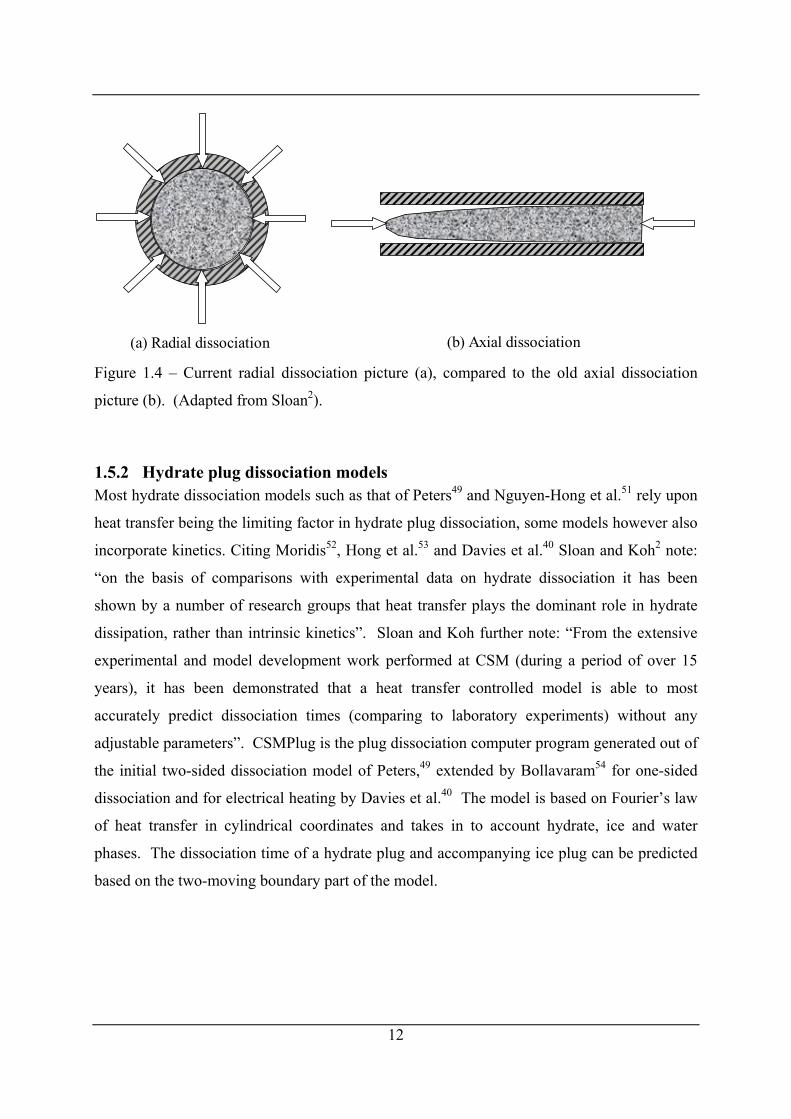
(a) Radial dissociation (b) Axial dissociation Figure 1.4 – Current radial dissociation picture (a), compared to the old axial dissociation
picture (b). (Adapted from Sloan2).
1.5.2 Hydrate plug dissociation models Most hydrate dissociation models such as that of Peters49 and Nguyen-Hong et al.51 rely upon
heat transfer being the limiting factor in hydrate plug dissociation, some models however also
incorporate kinetics. Citing Moridis52, Hong et al.53 and Davies et al.40 Sloan and Koh2 note:
“on the basis of comparisons with experimental data on hydrate dissociation it has been
shown by a number of research groups that heat transfer plays the dominant role in hydrate
dissipation, rather than intrinsic kinetics”. Sloan and Koh further note: “From the extensive
experimental and model development work performed at CSM (during a period of over 15
years), it has been demonstrated that a heat transfer controlled model is able to most
accurately predict dissociation times (comparing to laboratory experiments) without any
adjustable parameters”. CSMPlug is the plug dissociation computer program generated out of
the initial two-sided dissociation model of Peters,49 extended by Bollavaram54 for one-sided
dissociation and for electrical heating by Davies et al.40 The model is based on Fourier’s law
of heat transfer in cylindrical coordinates and takes in to account hydrate, ice and water
phases. The dissociation time of a hydrate plug and accompanying ice plug can be predicted
based on the two-moving boundary part of the model.
12
13
1.6 Structure and stoichiometry of semi-clathrate hydrates
1.6.1 Cage structure of semi-clathrate hydrates Semi-clathrate hydrates (SCH) of tetrabutylammonium (TBA) and tetraisopentylammonium
(TIPA) quaternary ammonium salts were discovered by Fowler et al. in 1940s.55 Since that
time other SCH have been discovered and structurally analysed by single crystal X-ray
crystallography such as those of trialkylsulfonium salts,56,57 tetraalkylphosphonium56 and
trialkylphosphine oxides.58 The first series of structural studies of SCH where published by
Jeffrey, McMullan and coworkers.5,57,59-61 In these structures, water lattice sites are replaced
by the cation centres and anions and each alkyl chains occupies a larger cage, which may be a
tetrakaidecahedral (51262), pentakaidecahedral (51263) or hexakaidecahedral (51264). Small
unoccupied dodecahedral (512) cages are interspaced between some of the large cages. The
breaking of the water lattice by the cation centres and anions lead Davidson11 to introduce the
term “semi-clathrate hydrates”. Figure 1.5 shows the structure of a tetra-n-butylammonium
bromide (TBAB) SCH with a hydrate number of 38 from Shimada et al.62 The centre of the
cation replaces a lattice site and the alkyl chains fill the larger cages as guests. The larger
cages in this structure are two tetrakaidecahedrons (51262) and two pentakaidecahedrons
(51263). The smaller dodecahedral (512) cages are filled with spheres to indicate that they
could be filled with suitably sized molecules. Indeed Shimada and coworkers63 as well as
Kamata et al.64 provided some of the first evidence that unoccupied cages in SCH could
enclathrate suitably sized molecules, namely methane, hydrogen sulfide and nitrogen when
they showed it was possible to separate these molecules from larger molecules such as ethane,
propane and carbon dioxide with tetrabutylammonium bromide SCHs. However McMullan
et al.61 had earlier noted the evolution of gas bubbles from melting tetrabutylammonium
fluoride crystals which was shown to be air by gas chromatography. Similar observation of
bubbling upon melting of SCH crystals were made by Jeffrey4 and Davidson.11 The
experiments by Stupin and Stravitnaya had also shown prior to Shimada et al. and Kamata et
al. that SCH of tetrabutylammonium bromide and acetate as well as tetrabutylammonium and
tetraisopentylammonium phthalates could adsorb sulfur dioxide.65,66
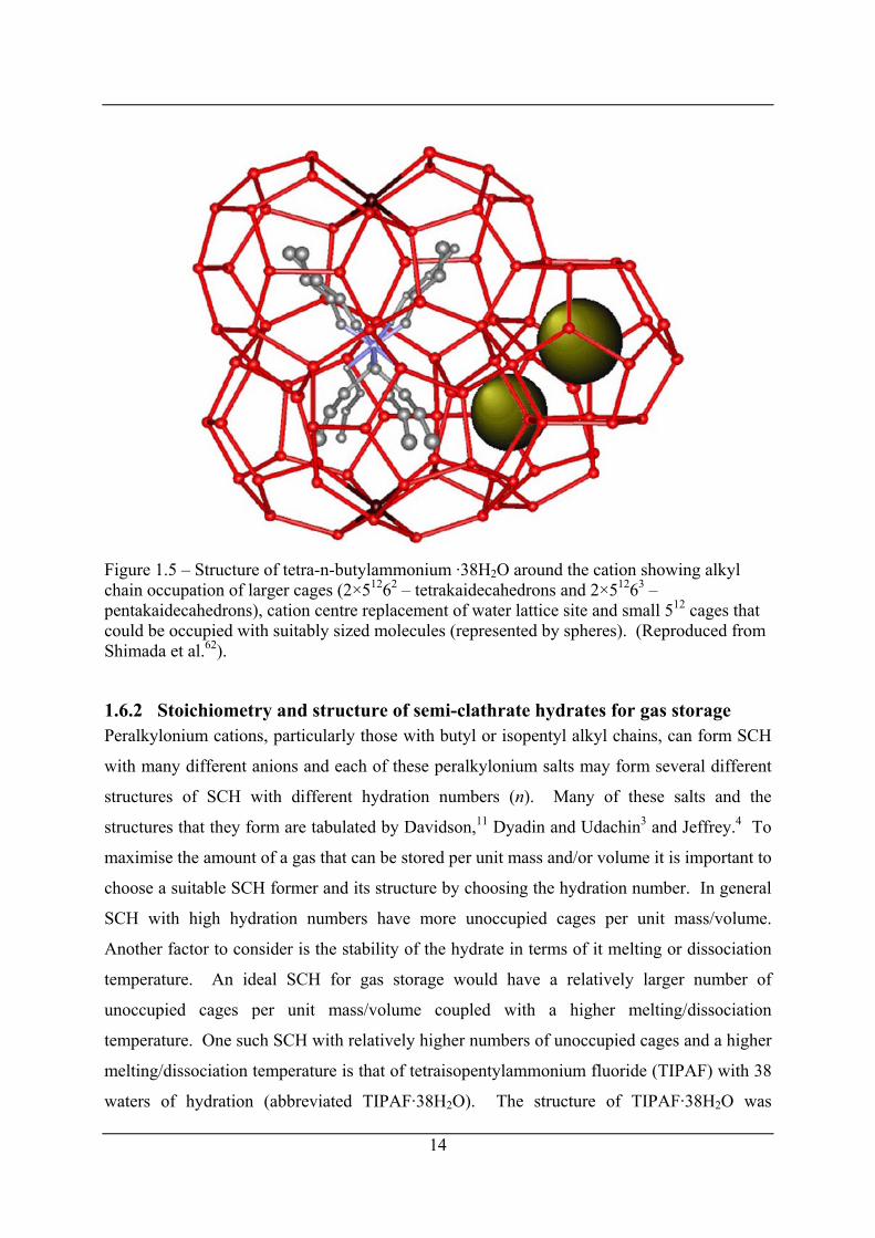
Figure 1.5 – Structure of tetra-n-butylammonium ·38H2O around the cation showing alkyl chain occupation of larger cages (2×51262 – tetrakaidecahedrons and 2×51263 – pentakaidecahedrons), cation centre replacement of water lattice site and small 512 cages that could be occupied with suitably sized molecules (represented by spheres). (Reproduced from Shimada et al.62).
1.6.2 Stoichiometry and structure of semi-clathrate hydrates for gas storage Peralkylonium cations, particularly those with butyl or isopentyl alkyl chains, can form SCH
with many different anions and each of these peralkylonium salts may form several different
structures of SCH with different hydration numbers (n). Many of these salts and the
structures that they form are tabulated by Davidson,11 Dyadin and Udachin3 and Jeffrey.4 To
maximise the amount of a gas that can be stored per unit mass and/or volume it is important to
choose a suitable SCH former and its structure by choosing the hydration number. In general
SCH with high hydration numbers have more unoccupied cages per unit mass/volume.
Another factor to consider is the stability of the hydrate in terms of it melting or dissociation
temperature. An ideal SCH for gas storage would have a relatively larger number of
unoccupied cages per unit mass/volume coupled with a higher melting/dissociation
temperature. One such SCH with relatively higher numbers of unoccupied cages and a higher
melting/dissociation temperature is that of tetraisopentylammonium fluoride (TIPAF) with 38
waters of hydration (abbreviated TIPAF·38H2O). The structure of TIPAF·38H2O was
14
15
determined by X-ray crystallography by Feil and Jeffrey.5 The structure is identical in cage
arrangement to the more recently analysed TBAB·38H2O SCH determined by Shimada et al.62
and partially illustrated in Figure 1.5. Figure 1.6 shows a T,w stability diagram for TIPAF +
water (where w1 is the mass fraction of the salt) reproduced from Lipkowski et al.67
Lipkowski et al. observed the TIPAF SCH with a hydration number of 38 that Feil and Jeffrey
had studied, as well as two other SCH with experimental hydration numbers of 26.8, and 32.7
(these hydration numbers were observed by both Karl Fischer titration for water content and
potentiometric titration of tetraphenylborate with an ion-selective electrode for the salt
concentration). Interestingly Lipkowski et al. noted that even though the TIPAF·38H2O
structure is metastable to the TIPAF·27H2O structure for much of the composition range
(greater than w1 ≈ 0.22) the TIPAF·38H2O hydrate was “repeatedly observed” indicating it
was kinetically favoured. The observation of the stable TIPAF·27H2O part of the diagram
was “only possible when freezing and melting of the mixture of the corresponding
composition was repeated many times until the metastable phases disappeared and the
mixture had been cooled to (-50 to -60) °C.”67 Crystals of the metastable TIPAF·32H2O
could only be grown “in the absence of any mechanical action or stirring in a [w1 ≈ 0.22]
solution at [(291.15 to 293.15) K]”.67 “Mechanical disturbance of the solution where
[TIPAF·32H2O] crystals were growing resulted in turbidity and the appearance of many tiny
[TIPAF·38H2O] crystals”.67 A full structural determination of the SCH with an experimental
hydration number of 26.8 was also presented by Lipkowski et al.67 to reveal a structural
stoichiometry of TIPAF·27H2O. In addition the space group for the SCH with experimental
hydration number of 32.7 was determined as P42/m. This space group is the same as that
determined for the SCH of tetra-n-butylammonium fluoride (TBAF) with a hydration number
of 32.8 whose crystal structure was determined by McMullan and Jeffrey,61 indicating
presumably similar structures. Details of each TIPAF SCH including stoichiometry,
crystallography, cage structure, and density are listed in Table 1.2 compiled largely from
Lipkowski et al.67 The geometry of the cages listed in Table 1.2 can be viewed in Figure 1.7.
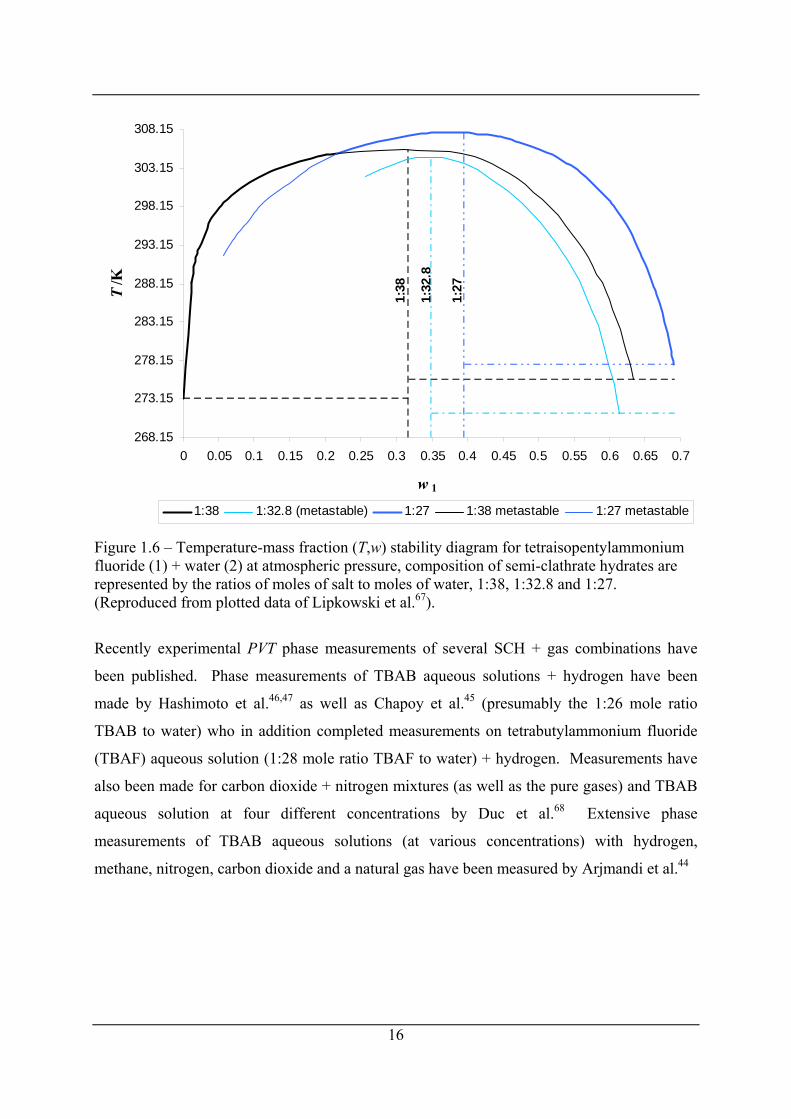
268.15
273.15
278.15
283.15
288.15
293.15
298.15
303.15
308.15
0 0.05 0.1 0.15 0.2 0.25 0.3 0.35 0.4 0.45 0.5 0.55 0.6 0.65 0.7
w 1
T/K
1:38 1:32.8 (metastable) 1:27 1:38 metastable 1:27 metastable
1:38
1:32
.8
1:27
Figure 1.6 – Temperature-mass fraction (T,w) stability diagram for tetraisopentylammonium fluoride (1) + water (2) at atmospheric pressure, composition of semi-clathrate hydrates are represented by the ratios of moles of salt to moles of water, 1:38, 1:32.8 and 1:27. (Reproduced from plotted data of Lipkowski et al.67).
Recently experimental PVT phase measurements of several SCH + gas combinations have
been published. Phase measurements of TBAB aqueous solutions + hydrogen have been
made by Hashimoto et al.46,47 as well as Chapoy et al.45 (presumably the 1:26 mole ratio
TBAB to water) who in addition completed measurements on tetrabutylammonium fluoride
(TBAF) aqueous solution (1:28 mole ratio TBAF to water) + hydrogen. Measurements have
also been made for carbon dioxide + nitrogen mixtures (as well as the pure gases) and TBAB
aqueous solution at four different concentrations by Duc et al.68 Extensive phase
measurements of TBAB aqueous solutions (at various concentrations) with hydrogen,
methane, nitrogen, carbon dioxide and a natural gas have been measured by Arjmandi et al.44
16
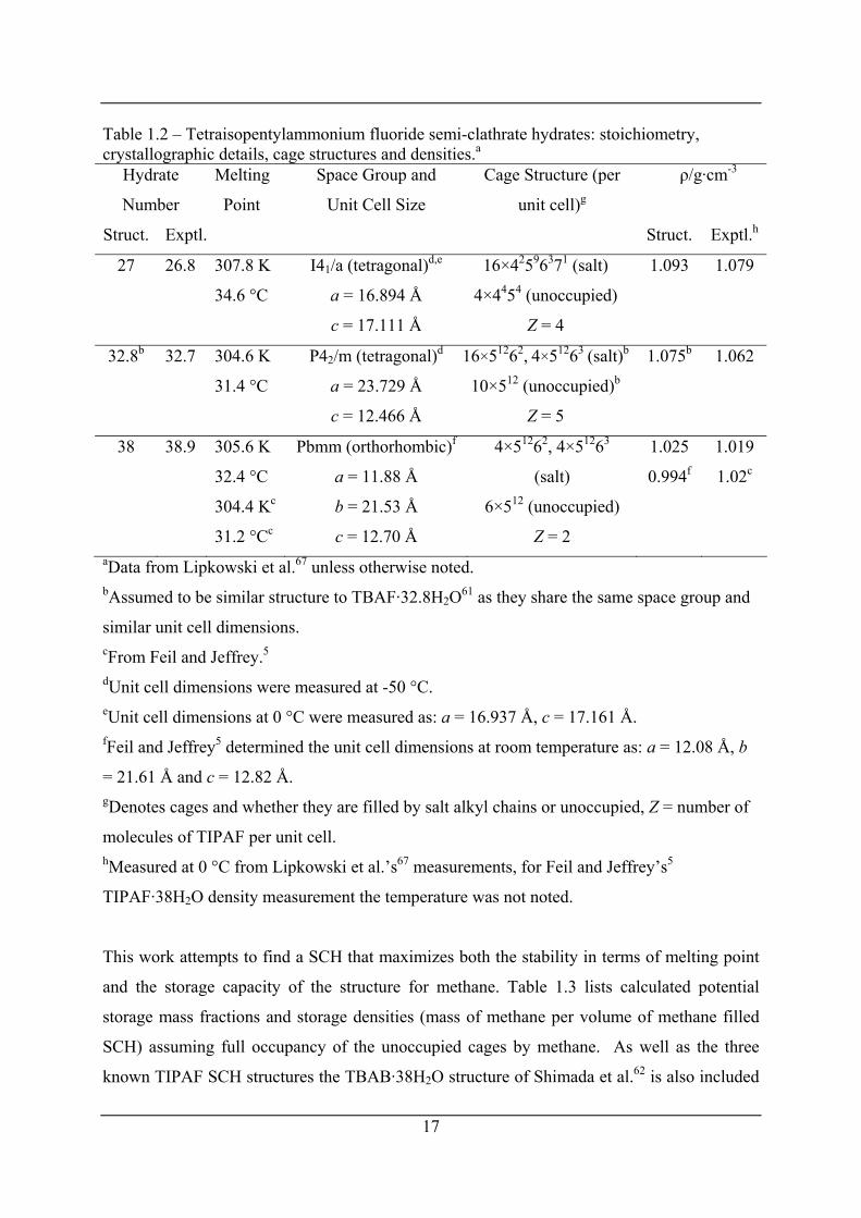
17
Table 1.2 – Tetraisopentylammonium fluoride semi-clathrate hydrates: stoichiometry, crystallographic details, cage structures and densities.a
Hydrate
Number
Melting
Point
Space Group and
Unit Cell Size
Cage Structure (per
unit cell)g
ρ/g·cm-3
Struct. Exptl. Struct. Exptl.h
27 26.8 307.8 K
34.6 °C
I41/a (tetragonal)d,e
a = 16.894 Å
c = 17.111 Å
16×42596371 (salt)
4×4454 (unoccupied)
Z = 4
1.093 1.079
32.8b 32.7 304.6 K
31.4 °C
P42/m (tetragonal)d
a = 23.729 Å
c = 12.466 Å
16×51262, 4×51263 (salt)b
10×512 (unoccupied)b
Z = 5
1.075b 1.062
38 38.9 305.6 K
32.4 °C
304.4 Kc
31.2 °Cc
Pbmm (orthorhombic)f
a = 11.88 Å
b = 21.53 Å
c = 12.70 Å
4×51262, 4×51263
(salt)
6×512 (unoccupied)
Z = 2
1.025
0.994f
1.019
1.02c
aData from Lipkowski et al.67 unless otherwise noted. bAssumed to be similar structure to TBAF·32.8H2O61 as they share the same space group and
similar unit cell dimensions. cFrom Feil and Jeffrey.5 dUnit cell dimensions were measured at -50 °C. eUnit cell dimensions at 0 °C were measured as: a = 16.937 Å, c = 17.161 Å. fFeil and Jeffrey5 determined the unit cell dimensions at room temperature as: a = 12.08 Å, b
= 21.61 Å and c = 12.82 Å. gDenotes cages and whether they are filled by salt alkyl chains or unoccupied, Z = number of
molecules of TIPAF per unit cell. hMeasured at 0 °C from Lipkowski et al.’s67 measurements, for Feil and Jeffrey’s5
TIPAF·38H2O density measurement the temperature was not noted.
This work attempts to find a SCH that maximizes both the stability in terms of melting point
and the storage capacity of the structure for methane. Table 1.3 lists calculated potential
storage mass fractions and storage densities (mass of methane per volume of methane filled
SCH) assuming full occupancy of the unoccupied cages by methane. As well as the three
known TIPAF SCH structures the TBAB·38H2O structure of Shimada et al.62 is also included
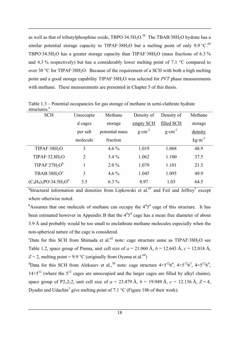
18
as well as that of tributylphosphine oxide, TBPO·34.5H2O.58 The TBAB·38H2O hydrate has a
similar potential storage capacity to TIPAF·38H2O but a melting point of only 9.9 °C.69
TBPO·34.5H2O has a greater storage capacity than TIPAF·38H2O (mass fractions of 6.3 %
and 4.3 % respectively) but has a considerably lower melting point of 7.1 °C compared to
over 30 °C for TIPAF·38H2O. Because of the requirement of a SCH with both a high melting
point and a good storage capability TIPAF·38H2O was selected for PVT phase measurements
with methane. These measurements are presented in Chapter 5 of this thesis.
Table 1.3 – Potential occupancies for gas storage of methane in semi-clathrate hydrate structures.a
SCH Unoccupie
d cages
per salt
molecule
Methane
storage
potential mass
fraction
Density of
empty SCH
g·cm-3
Density of
filled SCH
g·cm-3
Methane
storage
density
kg·m-3
TIPAF·38H2O 3 4.6 % 1.019 1.068 48.9
TIPAF·32.8H2O 2 3.4 % 1.062 1.100 37.5
TIPAF·27H2Ob 1 2.0 % 1.079 1.101 21.5
TBAB·38H2Oc 3 4.6 % 1.045 1.095 49.9
(C4H9)3PO·34.5H2Od 3.5 6.3 % 0.97 1.03 64.5 aStructural information and densities from Lipkowski et al.67 and Feil and Jeffrey5 except
where otherwise noted. bAssumes that one molecule of methane can occupy the 4454 cage of this structure. It has
been estimated however in Appendix B that the 4454 cage has a mean free diameter of about
3.9 Å and probably would be too small to enclathrate methane molecules especially when the
non-spherical nature of the cage is considered. cData for this SCH from Shimada et al.62 note: cage structure same as TIPAF·38H2O see
Table 1.2, space group of Pmma, unit cell size of a = 21.060 Å, b = 12.643 Å, c = 12.018 Å,
Z = 2, melting point = 9.9 °C (originally from Oyama et al.69) dData for this SCH from Alekseev et al.,58 note: cage structure 4×51264, 4×51263, 4×51264,
14×512 (where the 512 cages are unoccupied and the larger cages are filled by alkyl chains),
space group of P21212, unit cell size of a = 23.479 Å, b = 19.949 Å, c = 12.136 Å, Z = 4,
Dyadin and Udachin3 give melting point of 7.1 °C (Figure 18b of their work).
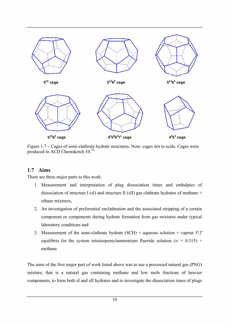
512 cage 51262 cage 51264 cage
51263 cage 42596371 cage 4454 cage Figure 1.7 – Cages of semi-clathrate hydrate structures; Note: cages not to scale. Cages were produced in ACD Chemsketch 10.70
1.7 Aims There are three major parts to this work:
1. Measurement and interpretation of plug dissociation times and enthalpies of
dissociation of structure I (sI) and structure II (sII) gas clathrate hydrates of methane +
ethane mixtures,
2. An investigation of preferential enclathration and the associated stripping of a certain
component or components during hydrate formation from gas mixtures under typical
laboratory conditions and
3. Measurement of the semi-clathrate hydrate (SCH) + aqueous solution + vapour P,T
equilibria for the system tetraisopentylammonium fluoride solution (w = 0.315) +
methane.
The aims of the first major part of work listed above was to use a processed natural gas (PNG)
mixture, that is a natural gas containing methane and low mole fractions of heavier
components, to form both sI and sII hydrates and to investigate the dissociation times of plugs
19
20
of these hydrates as well as their enthalpies of dissociation by calorimetry. PNGs have been
shown to form either a sI or sII hydrate depending on the pressure and temperature of hydrate
formation as well as the composition of the gas.54 Mixtures of methane + ethane have also
been shown to form either a sI or sII hydrate depending on the pressure and temperature of
hydrate formation as well as the composition of the gas.71,72 On this basis it was assumed that
methane + ethane mixtures were representative of PNGs. CSMPlug, a hydrate plug
dissociation prediction program developed by Peters49 at the Colorado School of Mines,
predicts that sII hydrate plugs of PNGs take approximately 30 % longer to dissociate than sI
hydrate plugs. An aim of this work was to test this prediction by experimental plug
dissociation time measurements. The CSMPlug prediction is based upon a larger dissociation
enthalpy for the sII hydrate than the sI hydrate (fixed values are assumed for each hydrate
structure, the gas composition and P and T are not taken into account). A further aim of this
section of work was to compare the measured enthalpies of dissociation to values predicted
from P,T phase data and the Clapeyron equation and to assess whether the enthalpies of
dissociation of the sII hydrates were always greater than the sI hydrates.
The second part of this work concerned the modelling of preferential enclathration.
Preferential enclathration is defined in this work as the preference of the hydrate phase to
enclathrate a certain component or components to a higher mole fraction on a water free basis
than in the gas phase. The preferential enclathration of components results in their depletion
or stripping from the gas phase. If the gas phase is constantly replenished as in a pipeline or a
system with a large mole ratio of gas to water then this preferential enclathration causes little
stripping in the gas phase. Typically the laboratory preparation of hydrate plugs involves the
supply of only just enough gas to ensure that all the initial ice or water is converted to hydrate
(low mole ratio of gas to water). For these typical laboratory systems it was hypothesised that
there could be significant stripping of the gas phase due to preferential enclathration. For
hydrate formation from methane + ethane mixtures it was also hypothesised that both sI and
sII hydrates may form due to a changing composition of the gas phase as hydrate formation
proceeded. The aim of this work was to produce stepwise models of the gas phase
composition as hydrate formation proceeded from melting ice (a typical laboratory hydrate
preparation method) and to validate these models against experimental measurements of the
21
gas phase composition as hydrate formation proceeded by the same method in a laboratory
pressure cell.
The third part of this work focused on P,T semi-clathrate hydrate (SCH) + aqueous + vapour
phase equilibria of tetraisopentylammonium fluoride solution (w = 0.315) + methane. The
aim of this work was to investigate the stability of this methane SCH as a function of
temperature and pressure and to compare the measurements to published results for the SCH
forming system tetrabutylammonium bromide solution (w = 0.30) + methane as well as pure
methane sI hydrate.
1.8 Thesis outline Chapter 2 entitled “Background to Instrumental and Analytical techniques” contain details of
each instrumental and analytical technique used in this work, including differential scanning
calorimetry (DSC), powder X-ray diffraction, Raman spectroscopy, Karl Fischer titration and
NMR spectroscopy. Where appropriate examples of the use of these techniques on gas
hydrates or SCHs is presented.
Chapter 3 discusses the fact that processed natural gases, low in components heavier than
methane, may form either sI or sII gas hydrates with water depending upon the pressure,
temperature and composition. Measurements of the dissociation time of sI and sII hydrate
plugs prepared in the laboratory from methane + ethane mixtures are presented and compared
to existing models of hydrate dissociation. An important parameter in hydrate dissociation
models is the enthalpy of dissociation of the hydrate. Measurements of the enthalpy of
dissociation from sII hydrates prepared from methane + ethane mixtures are presented and
compared both to the sI dissociation enthalpy of pure methane hydrate as well as predictions
of enthalpies of dissociation calculated from the Clapeyron equation. This chapter also
includes a literature review of laboratory hydrate plug formation experiments as well as gas
hydrate enthalpy of dissociation measurements and predictions using the Clapeyron equation.
Preferential enclathration occurs when a component of a gas mixture is enclathrated in the
hydrate phase on a water free basis to a higher mole fraction than in the free gas. This results
in the component being stripped from the free gas phase. Composition changes in the gases
22
may result in the formation of both sI and sII hydrates especially in systems where there is a
high mole ratio of water to gas, which are typical laboratory formation conditions. Chapter 4
presents models that consider preferential enclathration and the stripping of the free gas phase
for hydrate formations with gas mixtures. These models include a constant volume and a
constant pressure model. The constant volume model assumes an initial step pressurization of
a cell filled with ice particles. The formation of hydrates occurs by pressure drop when the
cell is heating just above ice’s melting point. The constant pressure model assumes that the
pressure in a cell containing slowly melting ice is maintained by compression of a syringe or
piston pump. The constant pressure model is compared to an experiment whereby the
composition of the gas was monitored as the hydrate formation proceeded.
In Chapter 5 SCH+Aq+V P,T equilibria measurements are presented for methane +
tetraisopentylammonium fluoride (TIPAF) in solution at a mole ratio of TIPAF·38.3H2O.
TIPAF was selected as the salt to study as it forms a SCH, TIPAF·38H2O, with a melting
point exceeding 30 °C and a relatively high number of unoccupied 512 cages per mole of salt.
TIPAF was unavailable commercially and therefore was prepared from triisopentylamine,
isopentyl bromide, and silver fluoride. A dilute solution of TIPAF was prepared and
crystallised SCH was filtered from the solution and tested for water content by Karl Fischer
titration, this confirmed a hydration number of 38.3 for the SCH. This SCH was used in
measurements of the P,T equilibria with methane in a pressure cell. These measurements are
compared to similar measurements conducted recently of tetrabutylammonium bromide
(TBAB) solution + methane SCH+Aq+V P,T equilibria.
Chapter 6 presents conclusions and recommendations for all the work encompassed in this
thesis as well as potential future work. Following Chapter 6 are references and appendices.
23
Chapter 2 BACKGROUND TO INSTRUMENTAL AND ANALYTICAL METHODS
In this work a variety of instrumental and analytical techniques have been used and applied to
the study of natural gas hydrates formed from methane and ethane gases and
tetraalkylammonium salt clathrate hydrates, namely tetraisopentylammonium fluoride
clathrates hydrates.
Differential scanning calorimetry (DSC) was used to study the enthalpies of dissociation of
(methane + ethane) gas hydrates of different structures (sI and sII). X-ray diffraction and
Raman spectroscopy were used to probe the structure of hydrate formed in the experiments
and gas liquid chromatography was used to analyse the gas composition of the hydrate phase
and gases used to form the hydrates.
Karl Fischer titrations were used to determine the hydration number of
tetraisopentylammonium fluoride hydrates formed. Nuclear magnetic resonance was used to
asses the purity of this salt that was prepared initially from a tertiary amine and alkyl halide.
2.1 Differential scanning calorimetry
2.1.1 DSC in this work Differential scanning calorimetry was used in this work to investigate the dissociation
enthalpies of sI and sII hydrates prepared from several different mixtures of methane and
ethane gases. The DSC used was a MC-DSC 4100 HT from Calorimetry Science Corporation
(now part of TA instruments) with a high pressure kit for measurements up to a pressure of
13.8 MPa.
2.1.2 Background to calorimetry Calorimetry is the science concerned with the measurement of the quantities of heat
exchanged. There are many different types of calorimeters available to measure calorimetric
or thermal properties and thermal events associated with physical processes and reactions.
These methods are discussed in detail in the IUPAC’s Experimental Thermodynamics
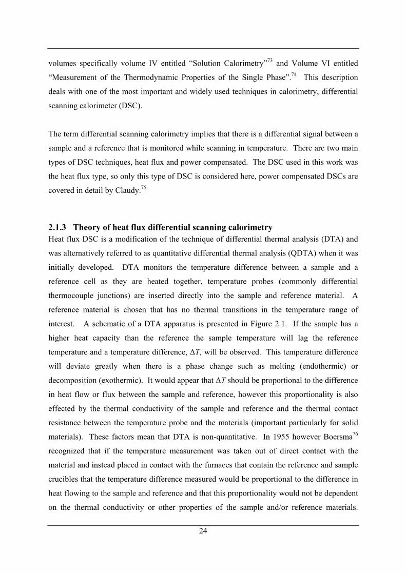
24
volumes specifically volume IV entitled “Solution Calorimetry”73 and Volume VI entitled
“Measurement of the Thermodynamic Properties of the Single Phase”.74 This description
deals with one of the most important and widely used techniques in calorimetry, differential
scanning calorimeter (DSC).
The term differential scanning calorimetry implies that there is a differential signal between a
sample and a reference that is monitored while scanning in temperature. There are two main
types of DSC techniques, heat flux and power compensated. The DSC used in this work was
the heat flux type, so only this type of DSC is considered here, power compensated DSCs are
covered in detail by Claudy.75
2.1.3 Theory of heat flux differential scanning calorimetry Heat flux DSC is a modification of the technique of differential thermal analysis (DTA) and
was alternatively referred to as quantitative differential thermal analysis (QDTA) when it was
initially developed. DTA monitors the temperature difference between a sample and a
reference cell as they are heated together, temperature probes (commonly differential
thermocouple junctions) are inserted directly into the sample and reference material. A
reference material is chosen that has no thermal transitions in the temperature range of
interest. A schematic of a DTA apparatus is presented in Figure 2.1. If the sample has a
higher heat capacity than the reference the sample temperature will lag the reference
temperature and a temperature difference, ΔT, will be observed. This temperature difference
will deviate greatly when there is a phase change such as melting (endothermic) or
decomposition (exothermic). It would appear that ΔT should be proportional to the difference
in heat flow or flux between the sample and reference, however this proportionality is also
effected by the thermal conductivity of the sample and reference and the thermal contact
resistance between the temperature probe and the materials (important particularly for solid
materials). These factors mean that DTA is non-quantitative. In 1955 however Boersma76
recognized that if the temperature measurement was taken out of direct contact with the
material and instead placed in contact with the furnaces that contain the reference and sample
crucibles that the temperature difference measured would be proportional to the difference in
heat flowing to the sample and reference and that this proportionality would not be dependent
on the thermal conductivity or other properties of the sample and/or reference materials.
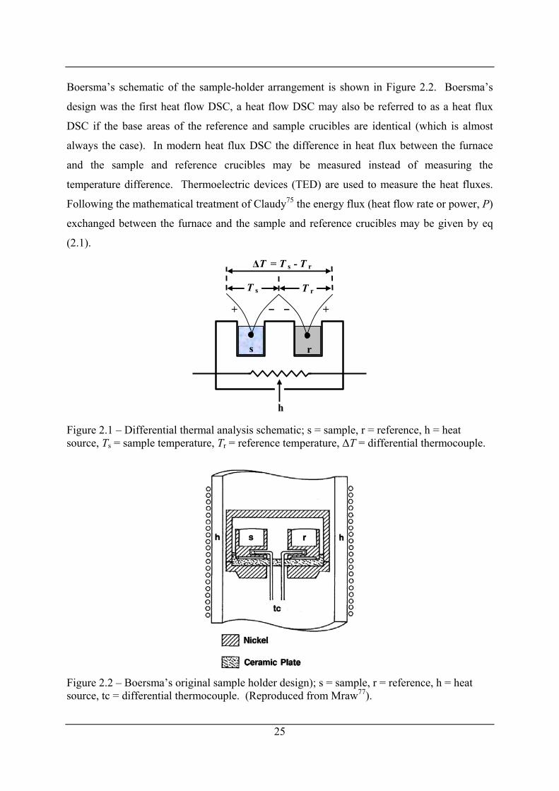
Boersma’s schematic of the sample-holder arrangement is shown in Figure 2.2. Boersma’s
design was the first heat flow DSC, a heat flow DSC may also be referred to as a heat flux
DSC if the base areas of the reference and sample crucibles are identical (which is almost
always the case). In modern heat flux DSC the difference in heat flux between the furnace
and the sample and reference crucibles may be measured instead of measuring the
temperature difference. Thermoelectric devices (TED) are used to measure the heat fluxes.
Following the mathematical treatment of Claudy75 the energy flux (heat flow rate or power, P)
exchanged between the furnace and the sample and reference crucibles may be given by eq
(2.1).
s r
T s T r
+ +– –
ΔT = T s - T r
h Figure 2.1 – Differential thermal analysis schematic; s = sample, r = reference, h = heat source, Ts = sample temperature, Tr = reference temperature, ΔT = differential thermocouple.
Figure 2.2 – Boersma’s original sample holder design); s = sample, r = reference, h = heat source, tc = differential thermocouple. (Reproduced from Mraw77).
25
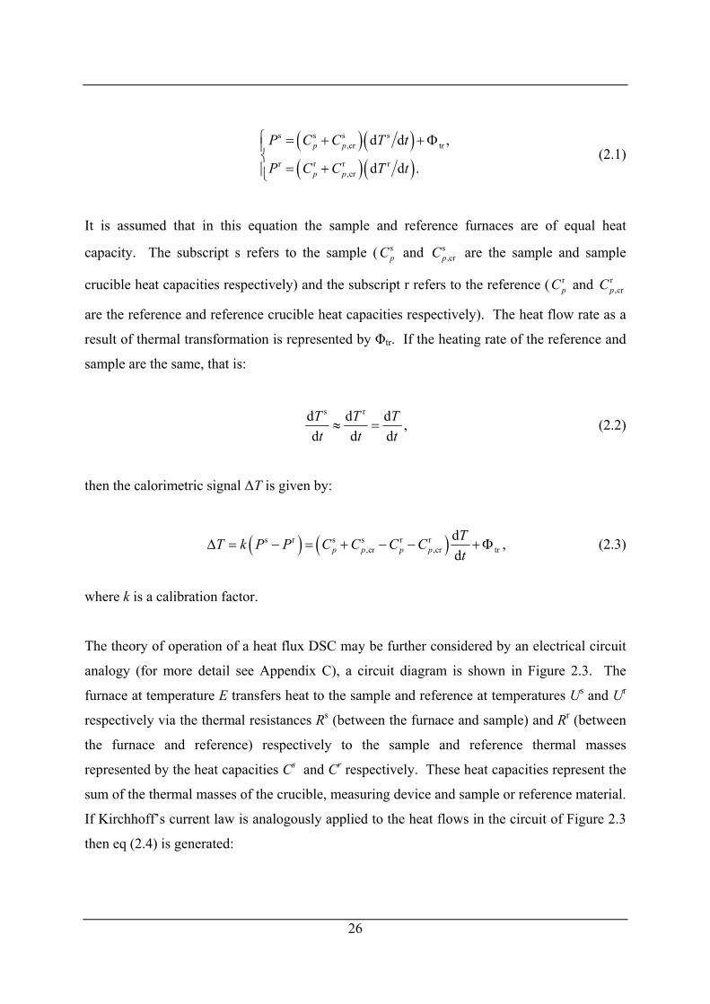
( )( )( )( )
s s s s,cr tr
r r r r,cr
d d
d d .
p p
p p
P C C T t
P C C T t
⎧ = + +Φ⎪⎨
= +⎪⎩
, (2.1)
It is assumed that in this equation the sample and reference furnaces are of equal heat
capacity. The subscript s refers to the sample ( and are the sample and sample
crucible heat capacities respectively) and the subscript r refers to the reference ( and
are the reference and reference crucible heat capacities respectively). The heat flow rate as a
result of thermal transformation is represented by Φtr. If the heating rate of the reference and
sample are the same, that is:
spC s
,crpC
rpC r
,crpC
s rd d d
d d dT Tt t≈ =
Tt
, (2.2)
then the calorimetric signal ΔT is given by:
( ) ( )s r s s r r,cr ,cr tr
ddp p p pTT k P P C C C Ct
Δ = − = + − − +Φ , (2.3)
where k is a calibration factor.
The theory of operation of a heat flux DSC may be further considered by an electrical circuit
analogy (for more detail see Appendix C), a circuit diagram is shown in Figure 2.3. The
furnace at temperature E transfers heat to the sample and reference at temperatures Us and Ur
respectively via the thermal resistances Rs (between the furnace and sample) and Rr (between
the furnace and reference) respectively to the sample and reference thermal masses
represented by the heat capacities Cs and Cr respectively. These heat capacities represent the
sum of the thermal masses of the crucible, measuring device and sample or reference material.
If Kirchhoff’s current law is analogously applied to the heat flows in the circuit of Figure 2.3
then eq (2.4) is generated:
26
s ss
trs
r rr
r
dd
dd
U E UCt R
U E UCt R
⎧ −= +Φ⎪⎪
⎨−⎪ =⎪⎩
(2.4)
Rs
Us
Ur Rr
E
Cs
Cr
Figure 2.3 – Electrical circuit equivalent of heat flux DSC; E = temperature of the furnace, Rs = thermal resistance between the furnace and sample, Rr = thermal resistance between the furnace and reference crucible, Us = temperature of the sample, Ur = temperature of the reference, Cs = heat capacity of the sample and crucible, and Cr = heat capacity of the reference and crucible. (Reproduced from Claudy75 in Goodwin et al.74).
The calorimetric signal ΔT is given by:
rT U U sΔ = − (2.5)
and may be determined by a “symmetric” instrument in which the resistance and heat
capacities of the sample and reference are approximately equal:
(2.6) s r
s r
, and.
R R RC C C
≈ =
≈ =
Combining eqs (2.4). (2.5) and (2.6) leads to:
trdd
T C TR tΔ Δ
Φ = + . (2.7)
27
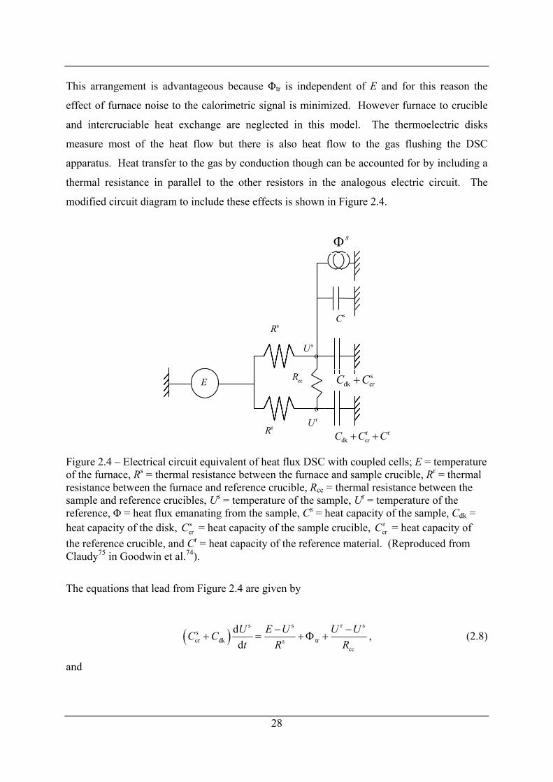
This arrangement is advantageous because Φtr is independent of E and for this reason the
effect of furnace noise to the calorimetric signal is minimized. However furnace to crucible
and intercruciable heat exchange are neglected in this model. The thermoelectric disks
measure most of the heat flow but there is also heat flow to the gas flushing the DSC
apparatus. Heat transfer to the gas by conduction though can be accounted for by including a
thermal resistance in parallel to the other resistors in the analogous electric circuit. The
modified circuit diagram to include these effects is shown in Figure 2.4.
sR
sU
rUrR
E s
dk crC C+
r rdk crC C C+ +
o
o
ccR
sΦ
sC
Figure 2.4 – Electrical circuit equivalent of heat flux DSC with coupled cells; E = temperature of the furnace, Rs = thermal resistance between the furnace and sample crucible, Rr = thermal resistance between the furnace and reference crucible, Rcc = thermal resistance between the sample and reference crucibles, Us = temperature of the sample, Ur = temperature of the reference, Φ = heat flux emanating from the sample, Cs = heat capacity of the sample, Cdk = heat capacity of the disk, = heat capacity of the sample crucible, = heat capacity of the reference crucible, and Cr = heat capacity of the reference material. (Reproduced from Claudy75 in Goodwin et al.74).
scrC r
crC
The equations that lead from Figure 2.4 are given by
( )s s r
scr dk trs
cc
ddU E U U UC Ct R R
−+ = +Φ +
s− , (2.8)
and
28
( )r r s
r rcr dk r
cc
ddU E U U UC C Ct R R
− −+ + = +
r
, (2.9)
where and are the heat capacities of the reference and sample crucibles respectively
and is the heat capacity of the thermoelectric disk. The thermal resistance between the
sample and reference crucibles is represented by Rcc.
rcrC
dk
scrC
C
Solving eqs (2.8) and (2.9) for Φtr assuming a symmetric calorimeter gives:
trcc
1 2 dd
TT CR R t
⎛ ⎞ ΔΦ = Δ + −⎜ ⎟
⎝ ⎠ (2.10)
This model only takes in to account first order effects, for a real instrument there may be
higher order effects which are included in an expansion of the form:
2
tr 1 2 3 2
d dd d
T Tk T k kt tΔ Δ
Φ = Δ + + +K (2.11)
where the values of the constants k1, k2, k3 etc are determined by calibration.
Other types and methods of DSC such as adiabatic DSC, single cell DSC and temperature
modulated DSC are discussed in detail by Claudy.75
2.1.4 Phase transition measurement by DSC When a phase transition is recorded, such as an enthalpy of fusion, by constant scan rate DSC
a large peak in the signal from the sample occurs. The signal can be plotted as a differential
power versus temperature chart, an example of which is shown in Figure 2.5. When a
baseline has been determined, the area between this baseline and the peak is proportional to
the enthalpy of transition (strictly speaking a scan with an empty crucible performed at the
same scan rate should be conducted first and this signal deducted to remove offset but this
29
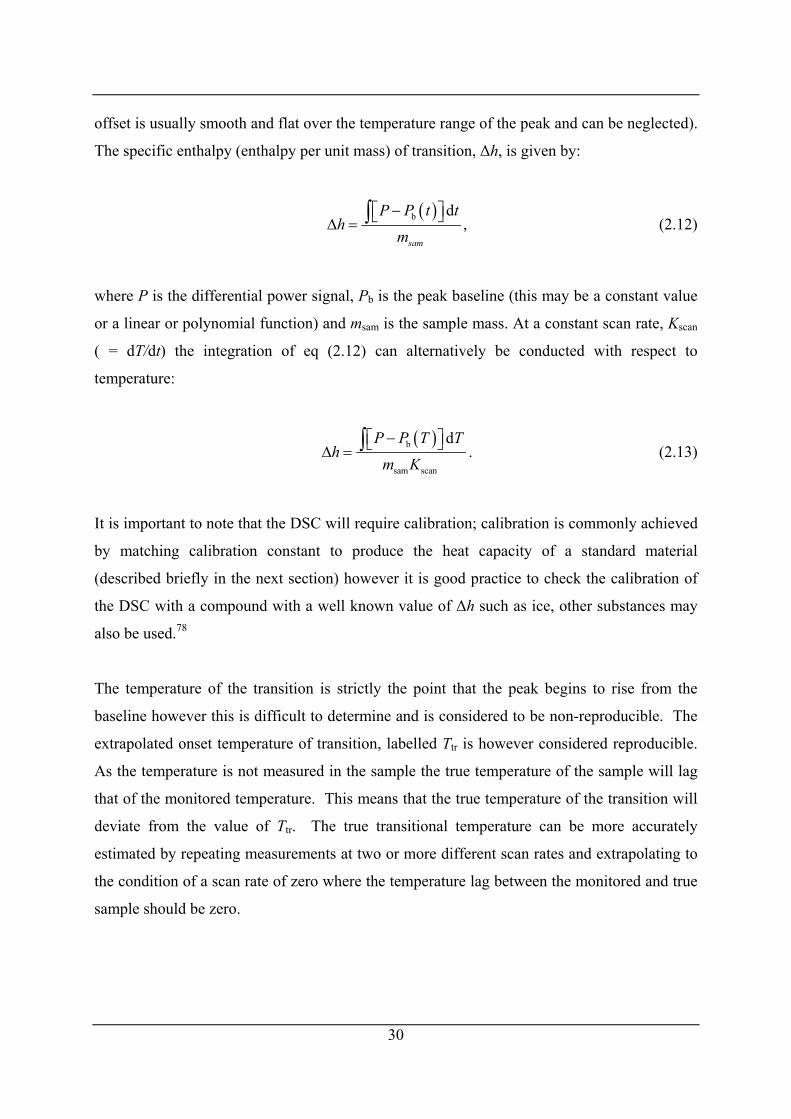
offset is usually smooth and flat over the temperature range of the peak and can be neglected).
The specific enthalpy (enthalpy per unit mass) of transition, Δh, is given by:
( )b d
sam
P P t th
m
−⎡ ⎤⎣ ⎦Δ = ∫ , (2.12)
where P is the differential power signal, Pb is the peak baseline (this may be a constant value
or a linear or polynomial function) and msam is the sample mass. At a constant scan rate, Kscan
( = dT/dt) the integration of eq (2.12) can alternatively be conducted with respect to
temperature:
( )b
sam scan
dP P T Th
m K
−⎡ ⎤⎣ ⎦Δ = ∫ . (2.13)
It is important to note that the DSC will require calibration; calibration is commonly achieved
by matching calibration constant to produce the heat capacity of a standard material
(described briefly in the next section) however it is good practice to check the calibration of
the DSC with a compound with a well known value of Δh such as ice, other substances may
also be used.78
The temperature of the transition is strictly the point that the peak begins to rise from the
baseline however this is difficult to determine and is considered to be non-reproducible. The
extrapolated onset temperature of transition, labelled Ttr is however considered reproducible.
As the temperature is not measured in the sample the true temperature of the sample will lag
that of the monitored temperature. This means that the true temperature of the transition will
deviate from the value of Ttr. The true transitional temperature can be more accurately
estimated by repeating measurements at two or more different scan rates and extrapolating to
the condition of a scan rate of zero where the temperature lag between the monitored and true
sample should be zero.
30
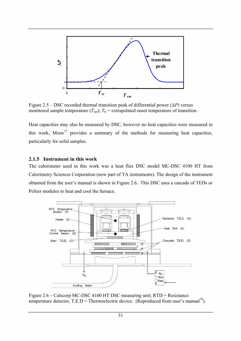
00 T sm
ΔPThermaltransition
peak
T tr
Figure 2.5 – DSC recorded thermal transition peak of differential power (ΔP) versus monitored sample temperature (Tsm); Ttr = extrapolated onset temperature of transition.
Heat capacities may also be measured by DSC, however no heat capacities were measured in
this work, Mraw77 provides a summary of the methods for measuring heat capacities,
particularly for solid samples.
2.1.5 Instrument in this work The calorimeter used in this work was a heat flux DSC model MC-DSC 4100 HT from
Calorimetry Sciences Corporation (now part of TA instruments). The design of the instrument
obtained from the user’s manual is shown in Figure 2.6. This DSC uses a cascade of TEDs or
Peltier modules to heat and cool the furnace.
Figure 2.6 – Calscorp MC-DSC 4100 HT DSC measuring unit; RTD = Resistance temperature detector, T.E.D = Thermoelectric device. (Reproduced from user’s manual79).
31
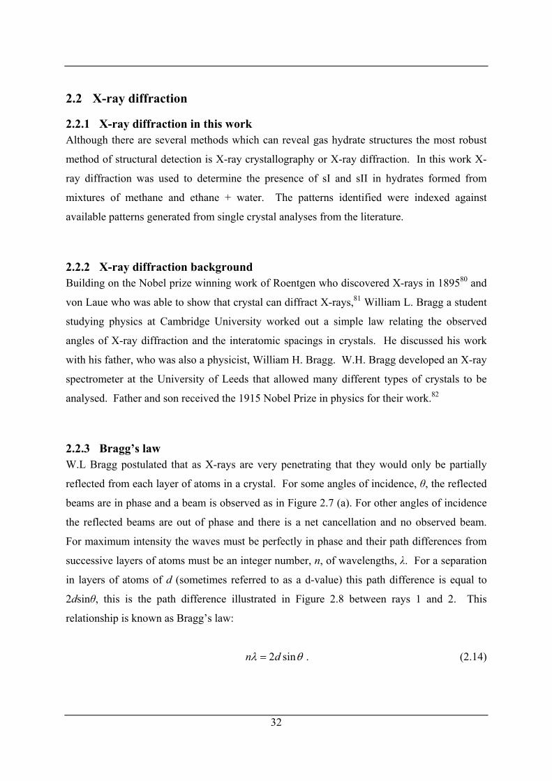
2.2 X-ray diffraction
2.2.1 X-ray diffraction in this work Although there are several methods which can reveal gas hydrate structures the most robust
method of structural detection is X-ray crystallography or X-ray diffraction. In this work X-
ray diffraction was used to determine the presence of sI and sII in hydrates formed from
mixtures of methane and ethane + water. The patterns identified were indexed against
available patterns generated from single crystal analyses from the literature.
2.2.2 X-ray diffraction background Building on the Nobel prize winning work of Roentgen who discovered X-rays in 189580 and
von Laue who was able to show that crystal can diffract X-rays,81 William L. Bragg a student
studying physics at Cambridge University worked out a simple law relating the observed
angles of X-ray diffraction and the interatomic spacings in crystals. He discussed his work
with his father, who was also a physicist, William H. Bragg. W.H. Bragg developed an X-ray
spectrometer at the University of Leeds that allowed many different types of crystals to be
analysed. Father and son received the 1915 Nobel Prize in physics for their work.82
2.2.3 Bragg’s law W.L Bragg postulated that as X-rays are very penetrating that they would only be partially
reflected from each layer of atoms in a crystal. For some angles of incidence, θ, the reflected
beams are in phase and a beam is observed as in Figure 2.7 (a). For other angles of incidence
the reflected beams are out of phase and there is a net cancellation and no observed beam.
For maximum intensity the waves must be perfectly in phase and their path differences from
successive layers of atoms must be an integer number, n, of wavelengths, λ. For a separation
in layers of atoms of d (sometimes referred to as a d-value) this path difference is equal to
2dsinθ, this is the path difference illustrated in Figure 2.8 between rays 1 and 2. This
relationship is known as Bragg’s law:
2 sinn dλ θ= . (2.14)
32
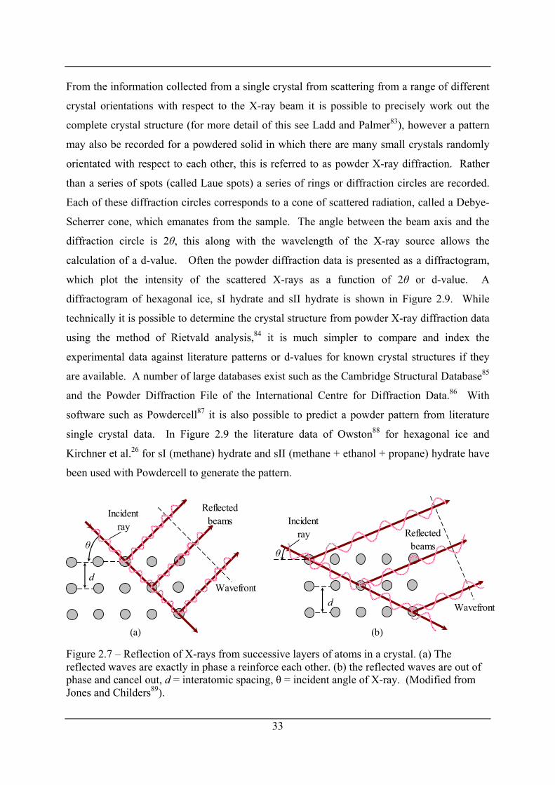
From the information collected from a single crystal from scattering from a range of different
crystal orientations with respect to the X-ray beam it is possible to precisely work out the
complete crystal structure (for more detail of this see Ladd and Palmer83), however a pattern
may also be recorded for a powdered solid in which there are many small crystals randomly
orientated with respect to each other, this is referred to as powder X-ray diffraction. Rather
than a series of spots (called Laue spots) a series of rings or diffraction circles are recorded.
Each of these diffraction circles corresponds to a cone of scattered radiation, called a Debye-
Scherrer cone, which emanates from the sample. The angle between the beam axis and the
diffraction circle is 2θ, this along with the wavelength of the X-ray source allows the
calculation of a d-value. Often the powder diffraction data is presented as a diffractogram,
which plot the intensity of the scattered X-rays as a function of 2θ or d-value. A
diffractogram of hexagonal ice, sI hydrate and sII hydrate is shown in Figure 2.9. While
technically it is possible to determine the crystal structure from powder X-ray diffraction data
using the method of Rietvald analysis,84 it is much simpler to compare and index the
experimental data against literature patterns or d-values for known crystal structures if they
are available. A number of large databases exist such as the Cambridge Structural Database85
and the Powder Diffraction File of the International Centre for Diffraction Data.86 With
software such as Powdercell87 it is also possible to predict a powder pattern from literature
single crystal data. In Figure 2.9 the literature data of Owston88 for hexagonal ice and
Kirchner et al.26 for sI (methane) hydrate and sII (methane + ethanol + propane) hydrate have
been used with Powdercell to generate the pattern.
d
θ
Incidentray
Reflectedbeams
Wavefrontd
θ
Incidentray Reflected
beams
Wavefront
(a) (b) Figure 2.7 – Reflection of X-rays from successive layers of atoms in a crystal. (a) The reflected waves are exactly in phase a reinforce each other. (b) the reflected waves are out of phase and cancel out, d = interatomic spacing, θ = incident angle of X-ray. (Modified from Jones and Childers89).
33
Figure 2.8 – Illustration of diffraction paths difference, maxima occur at angle where 2dsinθ is an integer multiple of wavelengths. (Reproduced from Jones and Childers89).
3.91
3.68 3.
45
8.40
5.94
5.31
4.85
4.20 3.
76
3.43
3.29
3.17
2.97
9.92
6.07
5.18
4.96
4.29
3.94 3.
51
3.31
3.04
03 4 5 6 7 8 9 10 11 12 13 1
2θ/°
Inte
nsity
(Arb
itrar
y U
nits
)
4
Hexagonal IcesI HydratesII Hydrate
Figure 2.9 – X-ray diffractogram for hexagonal ice, sI hydrate and sII hydrate; d-values in Ångströms are listed above the peaks, data generated using PowderCell87 using the data of Owston88 for hexagonal ice and Kirchner et al.26 for sI hydrate (methane hydrate) and sII hydrate (methane + ethanol + propane), λ = 0.70903165 Å.
34
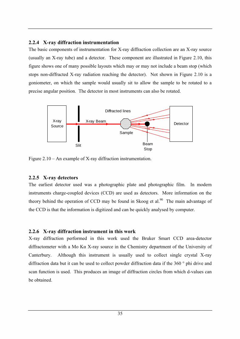
2.2.4 X-ray diffraction instrumentation The basic components of instrumentation for X-ray diffraction collection are an X-ray source
(usually an X-ray tube) and a detector. These component are illustrated in Figure 2.10, this
figure shows one of many possible layouts which may or may not include a beam stop (which
stops non-diffracted X-ray radiation reaching the detector). Not shown in Figure 2.10 is a
goniometer, on which the sample would usually sit to allow the sample to be rotated to a
precise angular position. The detector in most instruments can also be rotated.
X-raySource
Sample
Detector
BeamStop
X-ray Beam
Diffracted lines
Slit
Figure 2.10 – An example of X-ray diffraction instrumentation.
2.2.5 X-ray detectors The earliest detector used was a photographic plate and photographic film. In modern
instruments charge-coupled devices (CCD) are used as detectors. More information on the
theory behind the operation of CCD may be found in Skoog et al.90 The main advantage of
the CCD is that the information is digitized and can be quickly analysed by computer.
2.2.6 X-ray diffraction instrument in this work X-ray diffraction performed in this work used the Bruker Smart CCD area-detector
diffractometer with a Mo Kα X-ray source in the Chemistry department of the University of
Canterbury. Although this instrument is usually used to collect single crystal X-ray
diffraction data but it can be used to collect powder diffraction data if the 360 ° phi drive and
scan function is used. This produces an image of diffraction circles from which d-values can
be obtained.
35
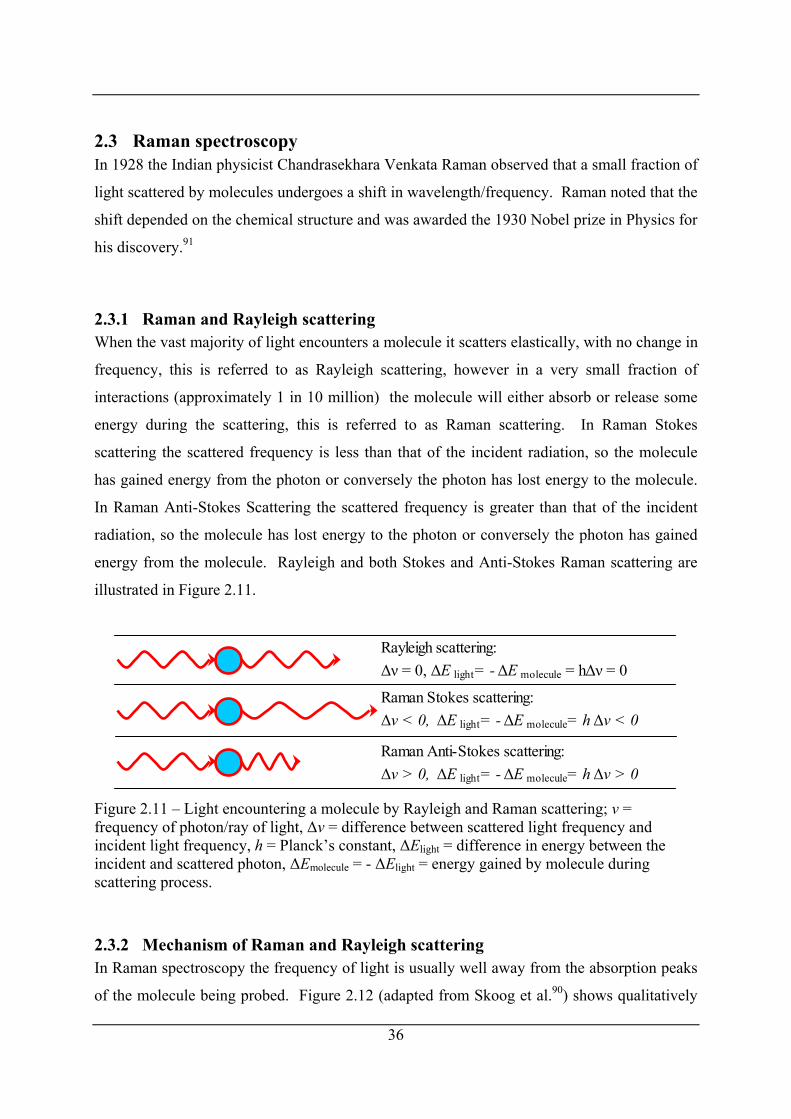
2.3 Raman spectroscopy In 1928 the Indian physicist Chandrasekhara Venkata Raman observed that a small fraction of
light scattered by molecules undergoes a shift in wavelength/frequency. Raman noted that the
shift depended on the chemical structure and was awarded the 1930 Nobel prize in Physics for
his discovery.91
2.3.1 Raman and Rayleigh scattering When the vast majority of light encounters a molecule it scatters elastically, with no change in
frequency, this is referred to as Rayleigh scattering, however in a very small fraction of
interactions (approximately 1 in 10 million) the molecule will either absorb or release some
energy during the scattering, this is referred to as Raman scattering. In Raman Stokes
scattering the scattered frequency is less than that of the incident radiation, so the molecule
has gained energy from the photon or conversely the photon has lost energy to the molecule.
In Raman Anti-Stokes Scattering the scattered frequency is greater than that of the incident
radiation, so the molecule has lost energy to the photon or conversely the photon has gained
energy from the molecule. Rayleigh and both Stokes and Anti-Stokes Raman scattering are
illustrated in Figure 2.11.
Rayleigh scattering: Δν = 0, ΔE light= -ΔE molecule = hΔν = 0
Raman Stokes scattering: Δν < 0, ΔE light= -ΔE molecule= hΔν < 0
Raman Anti-Stokes scattering: Δν > 0, ΔE light= -ΔE molecule= hΔν > 0
Figure 2.11 – Light encountering a molecule by Rayleigh and Raman scattering; ν = frequency of photon/ray of light, Δν = difference between scattered light frequency and incident light frequency, h = Planck’s constant, ΔElight = difference in energy between the incident and scattered photon, ΔEmolecule = - ΔElight = energy gained by molecule during scattering process.
2.3.2 Mechanism of Raman and Rayleigh scattering In Raman spectroscopy the frequency of light is usually well away from the absorption peaks
of the molecule being probed. Figure 2.12 (adapted from Skoog et al.90) shows qualitatively
36
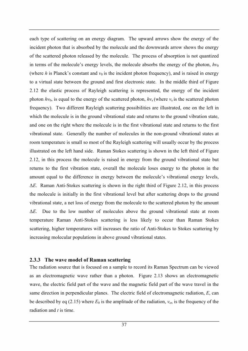
37
each type of scattering on an energy diagram. The upward arrows show the energy of the
incident photon that is absorbed by the molecule and the downwards arrow shows the energy
of the scattered photon released by the molecule. The process of absorption is not quantized
in terms of the molecule’s energy levels, the molecule absorbs the energy of the photon, hν0
(where h is Planck’s constant and ν0 is the incident photon frequency), and is raised in energy
to a virtual state between the ground and first electronic state. In the middle third of Figure
2.12 the elastic process of Rayleigh scattering is represented, the energy of the incident
photon hν0, is equal to the energy of the scattered photon, hνs (where νs is the scattered photon
frequency). Two different Rayleigh scattering possibilities are illustrated, one on the left in
which the molecule is in the ground vibrational state and returns to the ground vibration state,
and one on the right where the molecule is in the first vibrational state and returns to the first
vibrational state. Generally the number of molecules in the non-ground vibrational states at
room temperature is small so most of the Rayleigh scattering will usually occur by the process
illustrated on the left hand side. Raman Stokes scattering is shown in the left third of Figure
2.12, in this process the molecule is raised in energy from the ground vibrational state but
returns to the first vibration state, overall the molecule loses energy to the photon in the
amount equal to the difference in energy between the molecule’s vibrational energy levels,
ΔE. Raman Anti-Stokes scattering is shown in the right third of Figure 2.12, in this process
the molecule is initially in the first vibrational level but after scattering drops to the ground
vibrational state, a net loss of energy from the molecule to the scattered photon by the amount
ΔE. Due to the low number of molecules above the ground vibrational state at room
temperature Raman Anti-Stokes scattering is less likely to occur than Raman Stokes
scattering, higher temperatures will increases the ratio of Anti-Stokes to Stokes scattering by
increasing molecular populations in above ground vibrational states.
2.3.3 The wave model of Raman scattering The radiation source that is focused on a sample to record its Raman Spectrum can be viewed
as an electromagnetic wave rather than a photon. Figure 2.13 shows an electromagnetic
wave, the electric field part of the wave and the magnetic field part of the wave travel in the
same direction in perpendicular planes. The electric field of electromagnetic radiation, E, can
be described by eq (2.15) where E0 is the amplitude of the radiation, νex is the frequency of the
radiation and t is time.
( )0 cos 2π exE E ν= t . (2.15)
Raman Anti-Stokes
Scattering
ΔE = Energy between quantised vibrational levels
ΔE
RayleighScattering
Raman-Stokes
Scattering
1st electronic state
Ground Electronic State
0νh
Eh
ho
sΔ
−=
νν
0νh
0ν
νh
hs= 0νh
Eh
hs
Δ+
=0
νν
VirtualState
VirtualState
0νh
0ν
νh
hs=
ΔE
Figure 2.12 – Energy level diagram for Raman and Rayleigh Scattering. (Adapted from Skoog et al.90).
Wavelength (λ)
Electric Field (E )
Magnetic Field (B )
Direction ofPropagation
Figure 2.13 – The electromagnetic wave. (Adapted from Skoog et al.90).
38
When the electric field of the wave interacts with the electron cloud of the sample’s molecules
it induces a dipole moment, m, this is described by eq (2.16), where α is the polarizability (a
measure of the deformability of the molecule’s electron cloud):
( )0 cos 2πm E E tα α ν= = ex . (2.16)
To be Raman active the polarizability of the molecule’s bond must vary with the bond length.
Equation (2.17) describes the change in the polarizability with the bond length, where r is the
bond length, req is the equilibrium bond length and α0 is the polarizability when the bond
length is at is equilibrium length.
( )0 eqr rrαα α ∂
= + −∂
. (2.17)
The bond length varies with the frequency of vibration, νvib , by eq (2.18), where rm is the ratio
of the maximum bond length to equilibrium bond length:
( ) ( )eq m vibcos 2πr r r tν− = . (2.18)
Substituting eq (2.18) into eq (2.17) gives:
(0 m vicos 2πrr
)btαα α ν∂
= +∂
. (2.19)
Substituting eq (2.19) into eq (2.16) gives:
( ) ( ) (0 0 ex 0 m vib excos 2π cos 2π cos 2πm E t E r t tr
)αα ν ν ν∂= +
∂. (2.20)
By use of the trigonometric identity, eq (2.21), eq (2.20) can be rearranged to yield eq (2.22).
( ) ( ) ( ) ( )cos cos cos cos / 2x y x y x y= + + −⎡ ⎤⎣ ⎦ , (2.21)
39
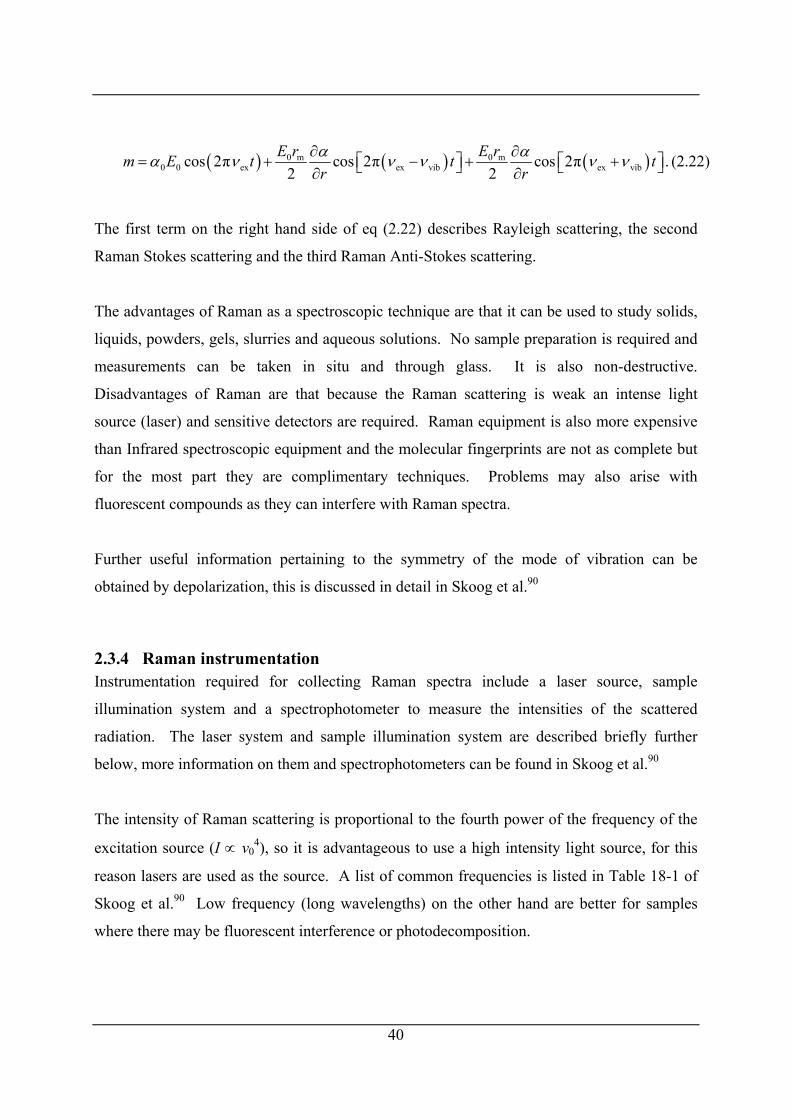
( ) ( ) ( )0 m 0 m0 0 ex ex vib ex vibcos 2π cos 2π cos 2π .
2 2E r E rm E t t t
r rα αα ν ν ν ν ν∂ ∂
= + − + +⎡ ⎤ ⎡ ⎤⎣ ⎦ ⎣∂ ∂ ⎦ (2.22)
The first term on the right hand side of eq (2.22) describes Rayleigh scattering, the second
Raman Stokes scattering and the third Raman Anti-Stokes scattering.
The advantages of Raman as a spectroscopic technique are that it can be used to study solids,
liquids, powders, gels, slurries and aqueous solutions. No sample preparation is required and
measurements can be taken in situ and through glass. It is also non-destructive.
Disadvantages of Raman are that because the Raman scattering is weak an intense light
source (laser) and sensitive detectors are required. Raman equipment is also more expensive
than Infrared spectroscopic equipment and the molecular fingerprints are not as complete but
for the most part they are complimentary techniques. Problems may also arise with
fluorescent compounds as they can interfere with Raman spectra.
Further useful information pertaining to the symmetry of the mode of vibration can be
obtained by depolarization, this is discussed in detail in Skoog et al.90
2.3.4 Raman instrumentation Instrumentation required for collecting Raman spectra include a laser source, sample
illumination system and a spectrophotometer to measure the intensities of the scattered
radiation. The laser system and sample illumination system are described briefly further
below, more information on them and spectrophotometers can be found in Skoog et al.90
The intensity of Raman scattering is proportional to the fourth power of the frequency of the
excitation source (I ∝ ν04), so it is advantageous to use a high intensity light source, for this
reason lasers are used as the source. A list of common frequencies is listed in Table 18-1 of
Skoog et al.90 Low frequency (long wavelengths) on the other hand are better for samples
where there may be fluorescent interference or photodecomposition.
40
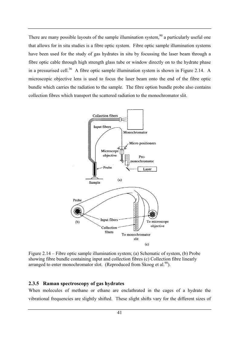
There are many possible layouts of the sample illumination system,90 a particularly useful one
that allows for in situ studies is a fibre optic system. Fibre optic sample illumination systems
have been used for the study of gas hydrates in situ by focussing the laser beam through a
fibre optic cable through high strength glass tube or window directly on to the hydrate phase
in a pressurised cell.36 A fibre optic sample illumination system is shown in Figure 2.14. A
microscopic objective lens is used to focus the laser beam onto the end of the fibre optic
bundle which carries the radiation to the sample. The fibre option bundle probe also contains
collection fibres which transport the scattered radiation to the monochromator slit.
Figure 2.14 – Fibre optic sample illumination system; (a) Schematic of system, (b) Probe showing fibre bundle containing input and collection fibres (c) Collection fibre linearly arranged to enter monochromator slot. (Reproduced from Skoog et al.90).
2.3.5 Raman spectroscopy of gas hydrates When molecules of methane or ethane are enclathrated in the cages of a hydrate the
vibrational frequencies are slightly shifted. These slight shifts vary for the different sizes of
41
cage. These shifts have been studied in detail for methane by Sum et al.92 and for methane +
ethane by Subramanian et al.36,71,72,93,94 Figure 2.15 from Subramanian et al.72 shows the
Raman wavenumber shifts in the C-H region of methane for hydrates prepared from mixtures
of methane + ethane gas. Although it is clear that there are differences in the Raman shifts for
methane in the small and large cages between sI and sII, the most easily obvious feature to
distinguish between the structures is the ratio of peak intensities. In the sI hydrates the peak
for the large 51262 cage (for which there are 6 per unit cell) is considerably greater in intensity
than the peak for the small 512 cage (for which there are 2 per unit cell). In the sII hydrates
the situation is reversed, with a larger peak for methane in the small cages rather than the
large cages, this is because there are more small 512 cages (16 per unit cell) than large 51264
cages (8 per unit cell).
Figure 2.15 – Raman spectra in the C-H region for hydrates formed from methane + ethane gas mixtures showing the slight differences in Raman shifts for enclathrated molecules in sI and sII hydrates. (Reproduced from Subramanian et al.72).
42
43
Raman spectroscopy in this work was used as a method to identify the structure of a methane
+ ethane gas hydrates as either sI or sII. The instrument used was a Renishaw Inc. MK III of
the Chemical Engineering department at the Colorado School of Mines. This instrument has
a 30 mW Argon laser (λ = 514.53 nm) and a 50 μm diameter fibre optic cable that transports
the light to a probe. A 20X objective lens is used to focus the laser beam. Back-scattered
light is collected by the probe and transported via collection fibres of the cable before passing
through a 2400 groove/mm diffraction grating to distribute the scattered light into its
component wavelengths. A charged coupled device (CCD) is used to record the spectra.
Calibration of the instrument was performed using the emission lines of Neon to give a
spectral accuracy of 0.3 cm-1, while the spectral resolution is 4.5 cm-1.
Raman spectroscopy was used in this work to determine if hydrates formed from a mixture of
methane + ethane gas were of sI or sII. This is presented in Chapter 3.
2.4 Gas liquid chromatography Gas liquid chromatography (GLC), sometimes simply referred to as Gas Chromatography
(GC), is a method of chromatographic separation for analytical purposes. The mobile phase is
a gas that is non-reactive with the sample, usually helium or nitrogen, the stationary phase is a
microscopic layer of liquid or polymer bound to an inert solid support inside a metal, glass or
ceramic column. This feasibility of this method of chromatography was suggested by Martin
and Synge95 in 1941, a GLC however was not built until about 10 years by James and
Martin.96,97 Martin and Synge received the 1952 Chemistry Nobel prize for the development
of partition chromatography.98
2.4.1 Basic principles of GLC If a sample of multiple components is introduced abruptly in to the carrier gas, each
component will distribute itself between the mobile carrier gas phase and the stationary phase
of liquid or polymer bound to an inert solid. Depending on the affinity of the sample
components for the stationary phase the components will be swept through the column in a
definite time, called the retention time. Other factors that affect the retention time include the
flow rate of carrier gas and the column temperature. The column temperature for most
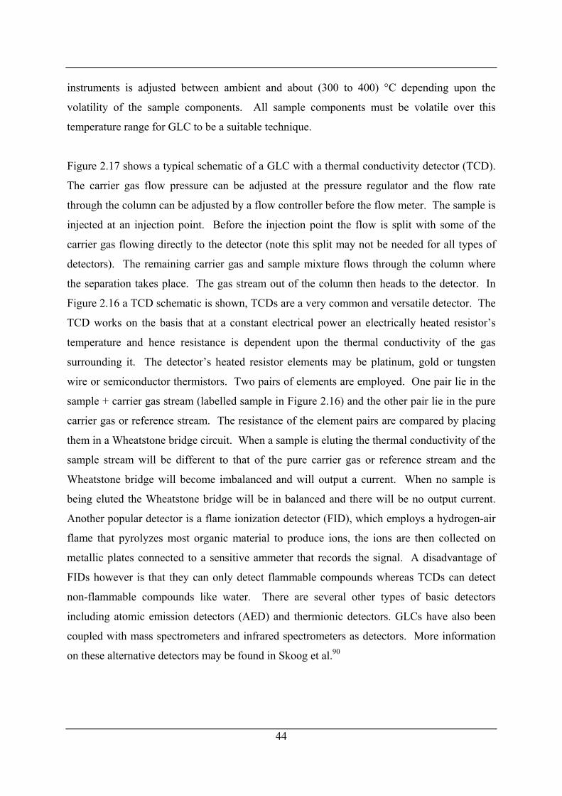
44
instruments is adjusted between ambient and about (300 to 400) °C depending upon the
volatility of the sample components. All sample components must be volatile over this
temperature range for GLC to be a suitable technique.
Figure 2.17 shows a typical schematic of a GLC with a thermal conductivity detector (TCD).
The carrier gas flow pressure can be adjusted at the pressure regulator and the flow rate
through the column can be adjusted by a flow controller before the flow meter. The sample is
injected at an injection point. Before the injection point the flow is split with some of the
carrier gas flowing directly to the detector (note this split may not be needed for all types of
detectors). The remaining carrier gas and sample mixture flows through the column where
the separation takes place. The gas stream out of the column then heads to the detector. In
Figure 2.16 a TCD schematic is shown, TCDs are a very common and versatile detector. The
TCD works on the basis that at a constant electrical power an electrically heated resistor’s
temperature and hence resistance is dependent upon the thermal conductivity of the gas
surrounding it. The detector’s heated resistor elements may be platinum, gold or tungsten
wire or semiconductor thermistors. Two pairs of elements are employed. One pair lie in the
sample + carrier gas stream (labelled sample in Figure 2.16) and the other pair lie in the pure
carrier gas or reference stream. The resistance of the element pairs are compared by placing
them in a Wheatstone bridge circuit. When a sample is eluting the thermal conductivity of the
sample stream will be different to that of the pure carrier gas or reference stream and the
Wheatstone bridge will become imbalanced and will output a current. When no sample is
being eluted the Wheatstone bridge will be in balanced and there will be no output current.
Another popular detector is a flame ionization detector (FID), which employs a hydrogen-air
flame that pyrolyzes most organic material to produce ions, the ions are then collected on
metallic plates connected to a sensitive ammeter that records the signal. A disadvantage of
FIDs however is that they can only detect flammable compounds whereas TCDs can detect
non-flammable compounds like water. There are several other types of basic detectors
including atomic emission detectors (AED) and thermionic detectors. GLCs have also been
coupled with mass spectrometers and infrared spectrometers as detectors. More information
on these alternative detectors may be found in Skoog et al.90
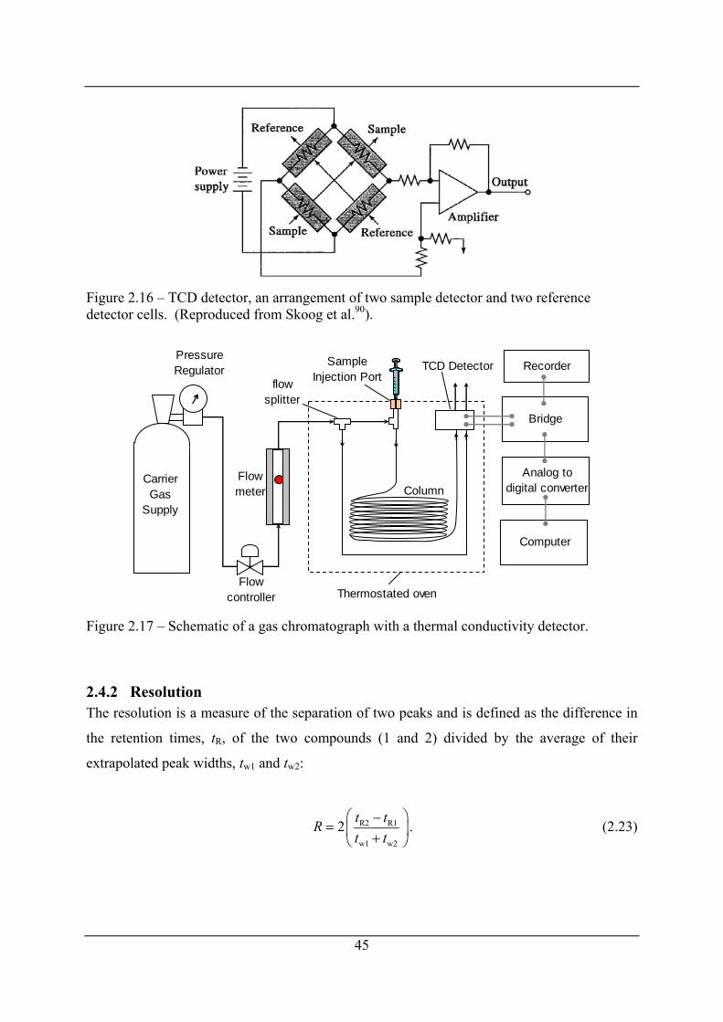
Figure 2.16 – TCD detector, an arrangement of two sample detector and two reference detector cells. (Reproduced from Skoog et al.90).
Analog to digital converter
Thermostated oven
CarrierGas
Supply
PressureRegulator
SampleInjection Port
TCD Detector
Bridge
Computer
Flowmeter Column
Flowcontroller
flowsplitter
Recorder
Figure 2.17 – Schematic of a gas chromatograph with a thermal conductivity detector.
2.4.2 Resolution The resolution is a measure of the separation of two peaks and is defined as the difference in
the retention times, tR, of the two compounds (1 and 2) divided by the average of their
extrapolated peak widths, tw1 and tw2:
R2 R1
w1 w2
2 t tRt t
⎛ ⎞−= ⎜ +⎝ ⎠
⎟ . (2.23)
45
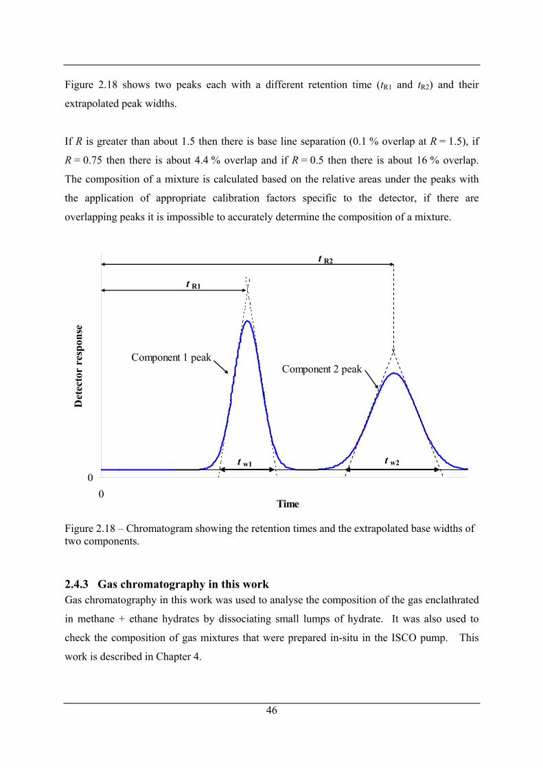
Figure 2.18 shows two peaks each with a different retention time (tR1 and tR2) and their
extrapolated peak widths.
If R is greater than about 1.5 then there is base line separation (0.1 % overlap at R = 1.5), if
R = 0.75 then there is about 4.4 % overlap and if R = 0.5 then there is about 16 % overlap.
The composition of a mixture is calculated based on the relative areas under the peaks with
the application of appropriate calibration factors specific to the detector, if there are
overlapping peaks it is impossible to accurately determine the composition of a mixture.
00
Time
Det
ecto
r re
spon
se
t w1
t R1
t R2
t w2
Component 1 peakComponent 2 peak
Figure 2.18 – Chromatogram showing the retention times and the extrapolated base widths of two components.
2.4.3 Gas chromatography in this work Gas chromatography in this work was used to analyse the composition of the gas enclathrated
in methane + ethane hydrates by dissociating small lumps of hydrate. It was also used to
check the composition of gas mixtures that were prepared in-situ in the ISCO pump. This
work is described in Chapter 4.
46
2.5 Karl Fischer titration In this work Karl Fischer titrations were used to measure the number of waters of
crystallization or hydrate number for the tetraalkylammonium salts. These results and
measured values are presented and discussed in Chapter 5.
Karl Fischer (KF) titration is an analytical titration method used to determine water content.
The method was developed by the German chemist Karl Fischer in 1935 when he realised it
was possible to use Bunsen’s reaction of iodine and sulfur dioxide (normally conducted in an
aqueous medium) for water determination in non-aqueous systems by using excess sulfur
dioxide.99 Fischer used a primary alcohol, methanol, and pyridine, a base, as the buffering
agent. Today the alcohol is still often methanol but also common is 2-(2-ethoxyethoxy)-
ethanol (also called diethylene glycol ethyl ether – DEGEE). The base used is most
commonly pyridine-free (as pyridine is a carcinogen) and tends to contain imidazole or
primary amines. The KF reaction is described by eqs (2.24) and (2.25):
[ ]2ROH + SO + R'N R'NH SO R→ 3 , (2.24)
alcohol base alkylsulfite
[ ] [ ] [ ]3 2 2 4R'NH SO R + H O + I + 2R'N R'NH SO R + 2 R'NH I→ . (2.25)
alkylsulfate hydroiodic acid salt
The KF titration method works upon the concentration of iodine. Iodine reacts with a 1:1
stoichiometry with water, once all the water has been consumed the excess iodine is detected
potentiometrically by the titrator’s indicator electrode (typically a double pin platinum
electrode) and this signifies the end point. The amount of water in the sample can be
calculated from the concentration of iodine in the KF reagent and the amount of KF reagent
consumed during the titration.
2.5.1 Karl Fischer titrators A Karl Fischer titration can be performed by a volumetric or coulometric method.100
Generally the volumetric method is best for water mass fractions from 1×10⁻⁴ to 1.0 whereas
47
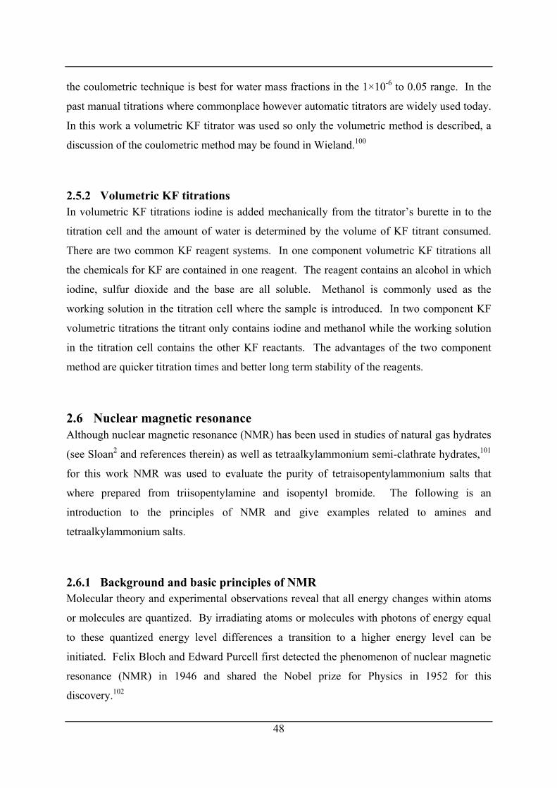
48
the coulometric technique is best for water mass fractions in the 1×10⁻⁶ to 0.05 range. In the
past manual titrations where commonplace however automatic titrators are widely used today.
In this work a volumetric KF titrator was used so only the volumetric method is described, a
discussion of the coulometric method may be found in Wieland.100
2.5.2 Volumetric KF titrations In volumetric KF titrations iodine is added mechanically from the titrator’s burette in to the
titration cell and the amount of water is determined by the volume of KF titrant consumed.
There are two common KF reagent systems. In one component volumetric KF titrations all
the chemicals for KF are contained in one reagent. The reagent contains an alcohol in which
iodine, sulfur dioxide and the base are all soluble. Methanol is commonly used as the
working solution in the titration cell where the sample is introduced. In two component KF
volumetric titrations the titrant only contains iodine and methanol while the working solution
in the titration cell contains the other KF reactants. The advantages of the two component
method are quicker titration times and better long term stability of the reagents.
2.6 Nuclear magnetic resonance Although nuclear magnetic resonance (NMR) has been used in studies of natural gas hydrates
(see Sloan2 and references therein) as well as tetraalkylammonium semi-clathrate hydrates,101
for this work NMR was used to evaluate the purity of tetraisopentylammonium salts that
where prepared from triisopentylamine and isopentyl bromide. The following is an
introduction to the principles of NMR and give examples related to amines and
tetraalkylammonium salts.
2.6.1 Background and basic principles of NMR Molecular theory and experimental observations reveal that all energy changes within atoms
or molecules are quantized. By irradiating atoms or molecules with photons of energy equal
to these quantized energy level differences a transition to a higher energy level can be
initiated. Felix Bloch and Edward Purcell first detected the phenomenon of nuclear magnetic
resonance (NMR) in 1946 and shared the Nobel prize for Physics in 1952 for this
discovery.102
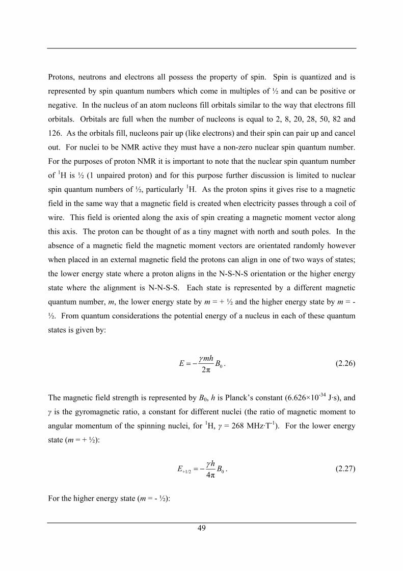
Protons, neutrons and electrons all possess the property of spin. Spin is quantized and is
represented by spin quantum numbers which come in multiples of ½ and can be positive or
negative. In the nucleus of an atom nucleons fill orbitals similar to the way that electrons fill
orbitals. Orbitals are full when the number of nucleons is equal to 2, 8, 20, 28, 50, 82 and
126. As the orbitals fill, nucleons pair up (like electrons) and their spin can pair up and cancel
out. For nuclei to be NMR active they must have a non-zero nuclear spin quantum number.
For the purposes of proton NMR it is important to note that the nuclear spin quantum number
of 1H is ½ (1 unpaired proton) and for this purpose further discussion is limited to nuclear
spin quantum numbers of ½, particularly 1H. As the proton spins it gives rise to a magnetic
field in the same way that a magnetic field is created when electricity passes through a coil of
wire. This field is oriented along the axis of spin creating a magnetic moment vector along
this axis. The proton can be thought of as a tiny magnet with north and south poles. In the
absence of a magnetic field the magnetic moment vectors are orientated randomly however
when placed in an external magnetic field the protons can align in one of two ways of states;
the lower energy state where a proton aligns in the N-S-N-S orientation or the higher energy
state where the alignment is N-N-S-S. Each state is represented by a different magnetic
quantum number, m, the lower energy state by m = + ½ and the higher energy state by m = -
½. From quantum considerations the potential energy of a nucleus in each of these quantum
states is given by:
02πmhE Bγ
= − . (2.26)
The magnetic field strength is represented by B0, h is Planck’s constant (6.626×10⁻³⁴ J·s), and
γ is the gyromagnetic ratio, a constant for different nuclei (the ratio of magnetic moment to
angular momentum of the spinning nuclei, for 1H, γ = 268 MHz·T-1). For the lower energy
state (m = + ½):
+1/2 04πhE Bγ
= − . (2.27)
For the higher energy state (m = - ½):
49
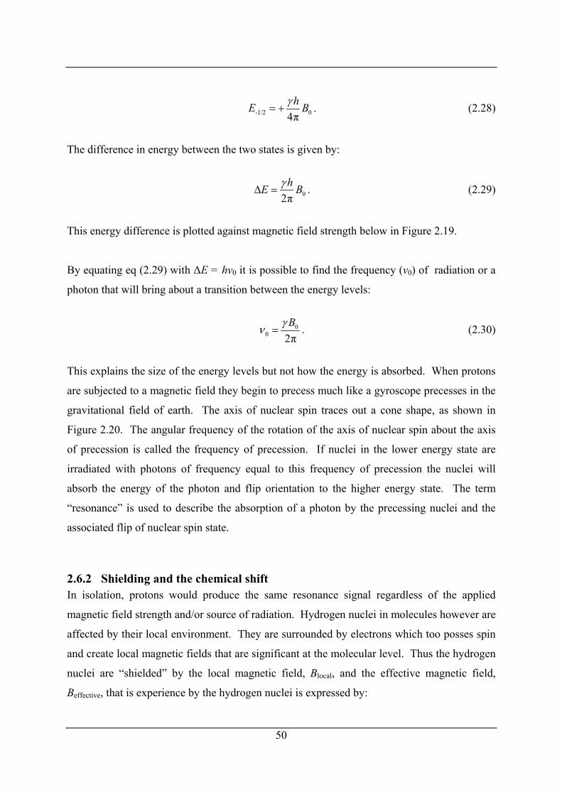
-1/2 04πhE Bγ
= + . (2.28)
The difference in energy between the two states is given by:
02πhE Bγ
Δ = . (2.29)
This energy difference is plotted against magnetic field strength below in Figure 2.19.
By equating eq (2.29) with ΔE = hν0 it is possible to find the frequency (ν0) of radiation or a
photon that will bring about a transition between the energy levels:
00 2π
Bγν = . (2.30)
This explains the size of the energy levels but not how the energy is absorbed. When protons
are subjected to a magnetic field they begin to precess much like a gyroscope precesses in the
gravitational field of earth. The axis of nuclear spin traces out a cone shape, as shown in
Figure 2.20. The angular frequency of the rotation of the axis of nuclear spin about the axis
of precession is called the frequency of precession. If nuclei in the lower energy state are
irradiated with photons of frequency equal to this frequency of precession the nuclei will
absorb the energy of the photon and flip orientation to the higher energy state. The term
“resonance” is used to describe the absorption of a photon by the precessing nuclei and the
associated flip of nuclear spin state.
2.6.2 Shielding and the chemical shift In isolation, protons would produce the same resonance signal regardless of the applied
magnetic field strength and/or source of radiation. Hydrogen nuclei in molecules however are
affected by their local environment. They are surrounded by electrons which too posses spin
and create local magnetic fields that are significant at the molecular level. Thus the hydrogen
nuclei are “shielded” by the local magnetic field, Blocal, and the effective magnetic field,
Beffective, that is experience by the hydrogen nuclei is expressed by:
50
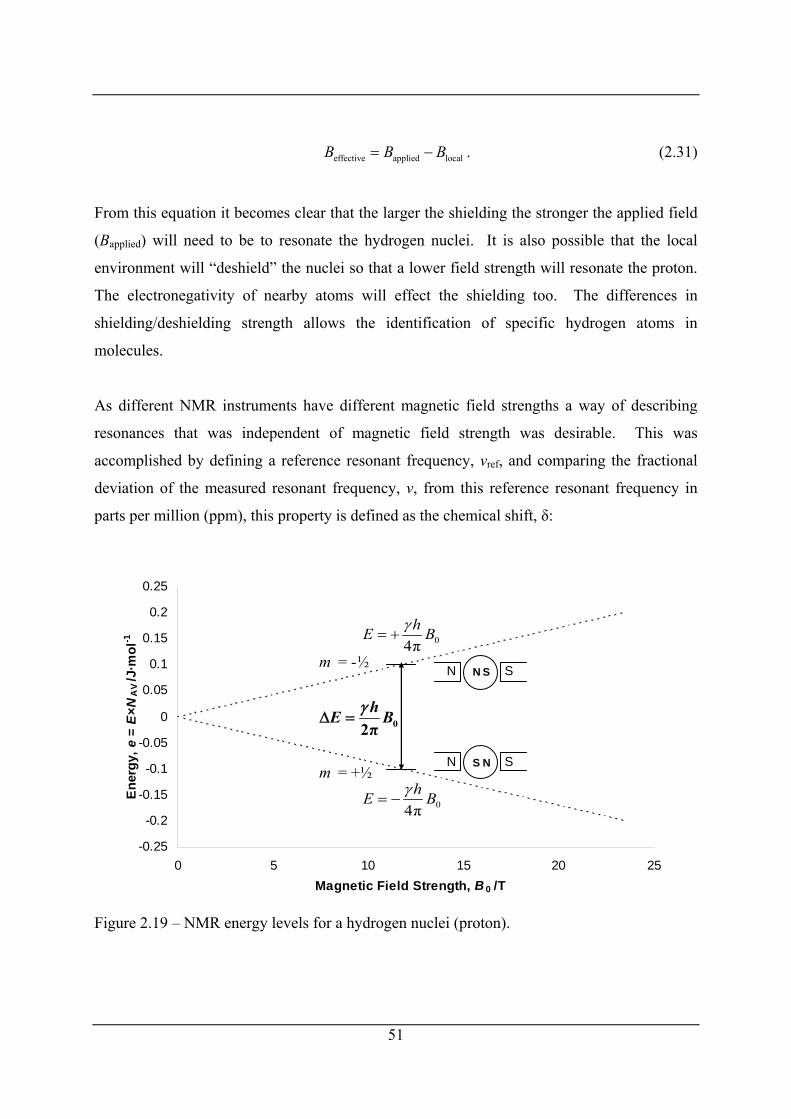
effective applied localB B B= − . (2.31)
From this equation it becomes clear that the larger the shielding the stronger the applied field
(Bapplied) will need to be to resonate the hydrogen nuclei. It is also possible that the local
environment will “deshield” the nuclei so that a lower field strength will resonate the proton.
The electronegativity of nearby atoms will effect the shielding too. The differences in
shielding/deshielding strength allows the identification of specific hydrogen atoms in
molecules.
As different NMR instruments have different magnetic field strengths a way of describing
resonances that was independent of magnetic field strength was desirable. This was
accomplished by defining a reference resonant frequency, νref, and comparing the fractional
deviation of the measured resonant frequency, ν, from this reference resonant frequency in
parts per million (ppm), this property is defined as the chemical shift, δ:
-0.25
-0.2
-0.15
-0.1
-0.05
0
0.05
0.1
0.15
0.2
0.25
0 5 10 15 20 25Magnetic Field Strength, B 0 /T
Ene
rgy,
e =
E×N
AV /
J·m
ol-1
N SN S
S NN Sm = +½
m = -½
02πhE Bγ
Δ =
04πhE Bγ
= +
04πhE Bγ
= −
Figure 2.19 – NMR energy levels for a hydrogen nuclei (proton).
51
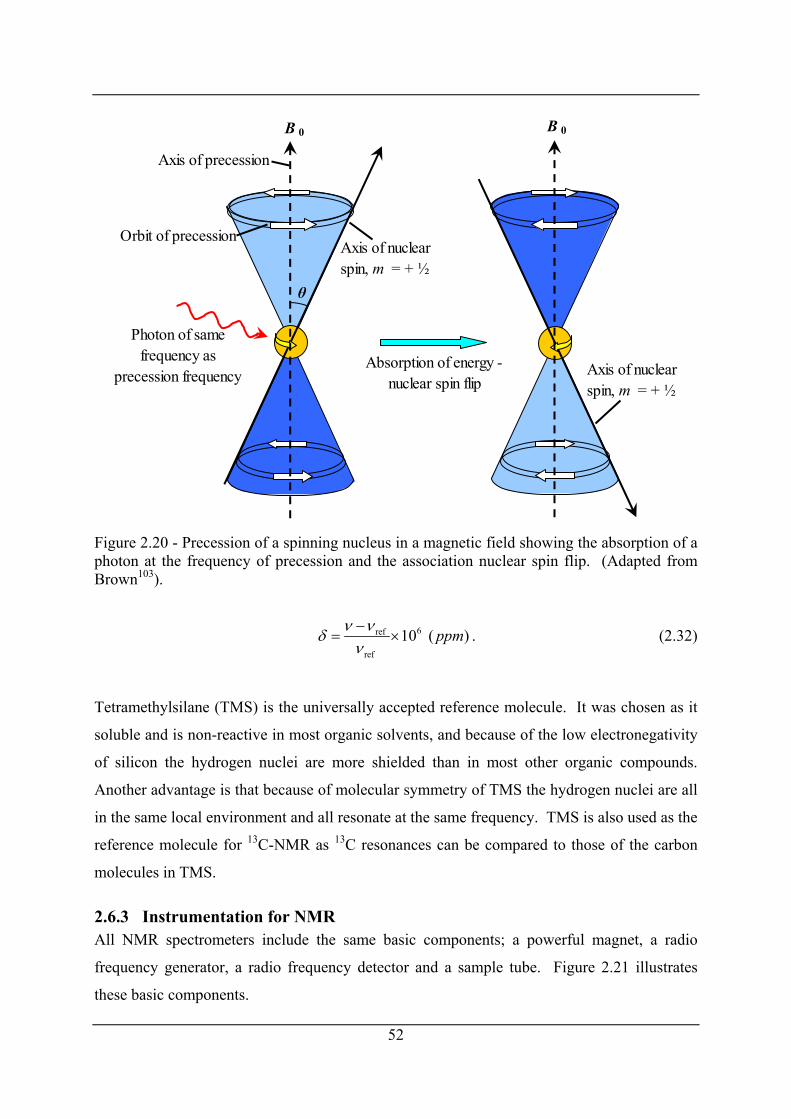
B 0 B 0
Axis of precession
Orbit of precession
Photon of samefrequency as
precession frequencyAbsorption of energy -
nuclear spin flip
Axis of nuclear spin, m = + ½
Axis of nuclearspin, m = + ½
θ
Figure 2.20 - Precession of a spinning nucleus in a magnetic field showing the absorption of a photon at the frequency of precession and the association nuclear spin flip. (Adapted from Brown103).
6ref
ref
10 ( )ppmν νδν−
= × . (2.32)
Tetramethylsilane (TMS) is the universally accepted reference molecule. It was chosen as it
soluble and is non-reactive in most organic solvents, and because of the low electronegativity
of silicon the hydrogen nuclei are more shielded than in most other organic compounds.
Another advantage is that because of molecular symmetry of TMS the hydrogen nuclei are all
in the same local environment and all resonate at the same frequency. TMS is also used as the
reference molecule for 13C-NMR as 13C resonances can be compared to those of the carbon
molecules in TMS.
2.6.3 Instrumentation for NMR All NMR spectrometers include the same basic components; a powerful magnet, a radio
frequency generator, a radio frequency detector and a sample tube. Figure 2.21 illustrates
these basic components.
52
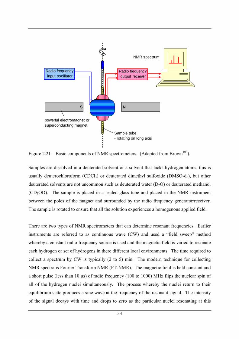
S N
Radio frequencyinput oscillator
Radio frequencyoutput receiver
NMR spectrum
powerful electromagnet orsuperconducting magnet
Sample tube - rotating on long axis
Figure 2.21 – Basic components of NMR spectrometers. (Adapted from Brown103).
Samples are dissolved in a deuterated solvent or a solvent that lacks hydrogen atoms, this is
usually deuterochloroform (CDCl3) or deuterated dimethyl sulfoxide (DMSO-d6), but other
deuterated solvents are not uncommon such as deuterated water (D2O) or deuterated methanol
(CD3OD). The sample is placed in a sealed glass tube and placed in the NMR instrument
between the poles of the magnet and surrounded by the radio frequency generator/receiver.
The sample is rotated to ensure that all the solution experiences a homogenous applied field.
There are two types of NMR spectrometers that can determine resonant frequencies. Earlier
instruments are referred to as continuous wave (CW) and used a “field sweep” method
whereby a constant radio frequency source is used and the magnetic field is varied to resonate
each hydrogen or set of hydrogens in there different local environments. The time required to
collect a spectrum by CW is typically (2 to 5) min. The modern technique for collecting
NMR spectra is Fourier Transform NMR (FT-NMR). The magnetic field is held constant and
a short pulse (less than 10 μs) of radio frequency (100 to 1000) MHz flips the nuclear spin of
all of the hydrogen nuclei simultaneously. The process whereby the nuclei return to their
equilibrium state produces a sine wave at the frequency of the resonant signal. The intensity
of the signal decays with time and drops to zero as the particular nuclei resonating at this
53

54
frequency reach their equilibrium state. This information is collected by computer and a
Fourier transform is applied that converts the intensity signals from a time-basis to a
frequency basis. The process of recording the spectra is typically 2 seconds or less. An
advantage of this technique is that a large number of repeated spectra can be recorded and
summed to give a time averaged spectra, this reduces noise while enhancing the spectra. It is
important to note however that some decay times can however be up 1 min and if the time
between sweeps is too short meaningless data will be obtained.
2.6.4 Peak areas The area of NMR spectra peaks are proportional to the number of hydrogen nuclei resonating
at that particular frequency, thus spectra are integrated to yield peak areas. This helps in
identifying the number of hydrogen atoms in each equivalent chemical environment.
2.6.5 NMR of amines and ammonium salts Table 2.1 lists the chemical shifts important for tertiary amine and quaternary ammonium salt
analysis. A more complete table including many other groups is available in Brown.103
Although the NMR spectra of tetraisopentylammonium ion in deuterated water (D2O) has
been studied by Harmon et al.104 and is listed in Table 2.2, it was not recorded at a high
enough resolution to give clearly individual peaks. For this reason the spectra of a similar
ion, the tetrahexylammonium ion is presented in Figure 2.22 as an example. The spectra of
the amine from which this salt would be prepared, trihexylamine, is shown in Figure 2.23.
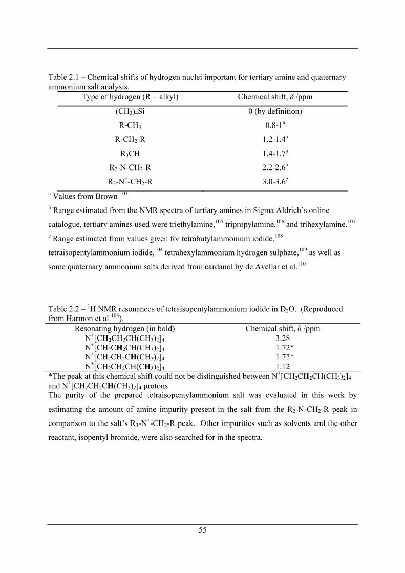
55
Table 2.1 – Chemical shifts of hydrogen nuclei important for tertiary amine and quaternary ammonium salt analysis.
Type of hydrogen (R = alkyl) Chemical shift, δ /ppm
(CH3)4Si 0 (by definition)
R-CH3 0.8-1a
R-CH2-R 1.2-1.4a
R3CH 1.4-1.7a
R2-N-CH2-R 2.2-2.6b
R3-N+-CH2-R 3.0-3.6c
a Values from Brown 103 b Range estimated from the NMR spectra of tertiary amines in Sigma Aldrich’s online
catalogue, tertiary amines used were triethylamine,105 tripropylamine,106 and trihexylamine.107 c Range estimated from values given for tetrabutylammonium iodide,108
tetraisopentylammonium iodide,104 tetrahexylammonium hydrogen sulphate,109 as well as
some quaternary ammonium salts derived from cardanol by de Avellar et al.110
Table 2.2 – 1H NMR resonances of tetraisopentylammonium iodide in D2O. (Reproduced from Harmon et al.104).
Resonating hydrogen (in bold) Chemical shift, δ /ppm N+[CH2CH2CH(CH3)2]4 3.28 N+[CH2CH2CH(CH3)2]4 1.72* N+[CH2CH2CH(CH3)2]4 1.72* N+[CH2CH2CH(CH3)2]4 1.12
*The peak at this chemical shift could not be distinguished between N+[CH2CH2CH(CH3)2]4 and N+[CH2CH2CH(CH3)2]4 protons The purity of the prepared tetraisopentylammonium salt was evaluated in this work by
estimating the amount of amine impurity present in the salt from the R2-N-CH2-R peak in
comparison to the salt’s R3-N+-CH2-R peak. Other impurities such as solvents and the other
reactant, isopentyl bromide, were also searched for in the spectra.
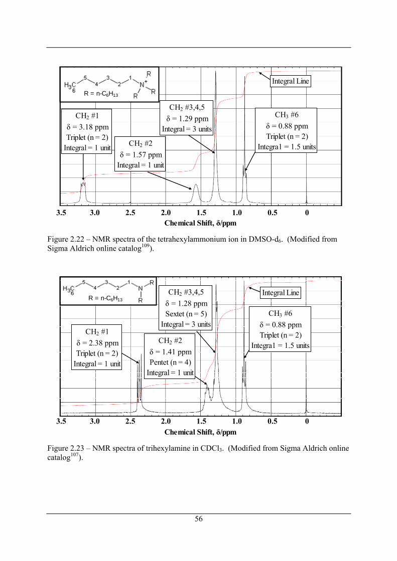
R = n-C6H13
Integral Line
CH3 #6δ = 0.88 ppmTriplet (n = 2)
Integra1 = 1.5 units
CH2 #3,4,5δ = 1.29 ppm
Integral = 3 units
CH2 #2δ = 1.57 ppm
Integral = 1 unit
CH2 #1δ = 3.18 ppmTriplet (n = 2)
Integral = 1 unit
3.5 3.0 2.5 2.0 1.5 1.0 0.5 0 Chemical Shift, δ/ppm
Figure 2.22 – NMR spectra of the tetrahexylammonium ion in DMSO-d6. (Modified from Sigma Aldrich online catalog109).
Integral Line
CH3 #6δ = 0.88 ppmTriplet (n = 2)
Integra1 = 1.5 units
CH2 #3,4,5δ = 1.28 ppmSextet (n = 5)
Integral = 3 units
CH2 #2δ = 1.41 ppmPentet (n = 4)
Integral = 1 unit
CH2 #1δ = 2.38 ppmTriplet (n = 2)
Integral = 1 unit
3.5 3.0 2.5 2.0 1.5 1.0 0.5 0 Chemical Shift, δ/ppm
R = n-C6H13
Figure 2.23 – NMR spectra of trihexylamine in CDCl3. (Modified from Sigma Aldrich online catalog107).
56
57
Chapter 3 PLUG DISSOCIATION TIMES AND ENTHALPIES OF DISSOCIATION OF SI AND SII GAS HYDRATES PREPARED FROM
METHANE + ETHANE MIXTURES
3.1 Introduction Methane rich natural gases, particularly those that are lean in propane and heavier
components, may form either a structure I (sI) or structure II (sII) clathrate hydrates in the
presence of water. The structure of hydrate is not only dependent on the composition of the
gas but also on the pressure-temperature (P,T) conditions. A model of two sided
depressurization of hydrates developed by Peters49 suggests that the structure of hydrate has a
strong effect on the dissociation time. The model predicts that the dissociation of a sII plug
will take approximately 30 % longer than for a sI plug. As hydrate dissociation is
endothermic, the dissociated water will often freeze to form an ice plug even when ambient
conditions are above 0 °C. Taking this into account the model predicts that removal of a
hydrate and ice will take about 20 % longer for the sII plug than the sI plug. The aim of this
research was to quantify whether these predictions were correct by calorimetric measurements
of enthalpies of dissociation as well as direct plug dissociation time measurements. Mixtures
of methane + ethane were used to prepare hydrates of sI and sII. Parts of this section were
published in a recent GPA research report.111
A literature review is presented discussing methane + ethane hydrates and the fact that despite
the pure gases only forming sI hydrates, certain mixtures of the two gases form sII hydrates.
Published experimental measurements as well as reasoning on why certain mixtures form sII
hydrates are presented. Structure I to structure II transitions of hydrates formed by processed
natural gases are also discussed. A review of laboratory hydrate plug formation and the
modelling of the dissociation of hydrate plugs then follow. Finally the enthalpy of
dissociation of gas hydrates is discussed. Calorimetric measurements as well as the use of the
Clapeyron equation for their calculation are reviewed.
58
Experimental work is then presented. The preparation of methane + ethane mixtures as well
as measurements of plug dissociation times, hydrate structure identification by X-ray
diffraction and Raman spectroscopy, and calorimetric measurements are included.
Results then follow, firstly P,x hydrate phase diagrams for methane + ethane mixtures,
calculated using the hydrate prediction program CSMGem, at low water to gas mole ratios
typical of the conditions in natural gas pipelines are presented. The problem of preferential
enclathration is introduced for consideration when preparing hydrate plugs in the laboratory, a
calculation algorithm for pressure drop hydrate formations is presented and a calculation is
illustrated for a high methane mole fraction mixture of methane + ethane. Methane + ethane
P,T phase diagrams for the mixtures prepared in this work at a high mole ratio of gas to water
are then presented. The results of the plug dissociation measurements including the structural
analyses of the hydrates formed then follow. Next calorimetric measurements of the
enthalpies of dissociation for a sII hydrate formed from a mixture of mole fraction 98.8 %
methane + 1.2 % ethane are presented along with Clapeyron calculated enthalpies of
dissociation for methane + ethane sI and sII hydrates. Finally CSMGem based predictions of
the average guest size in each cage of sI and sII methane + ethane hydrates of a mixture of
mole fraction 65.4 % methane + 34.6 % ethane are presented. The results are then considered
in the discussion.
3.2 Review of literature
3.2.1 Structure I to Structure II transitions in double guest hydrates Molecules that are of van der Waals diameter of approximately 6 Å, are of size close to the
point in which they are two big to stabilize the 51262 cage of sI and will instead stabilize the
51264 cage of sII. Two molecules of about this size, cyclopropane112 (5.9 Å) and trimethylene
oxide113 (6.1 Å) have been shown to form both sI and sII hydrates depending upon the
pressure, temperature and composition. More unusually however certain binary mixtures of
hydrate formers that as single guest components form sI hydrates have been shown to form sII
double guest hydrates. This effect was first observed in the mid-1950’s by von Stackelberg
and Jahn114 who measured sII sized lattice parameters by X-ray diffraction for binary mixtures
of H2S and CH3Br, COS, and CHF2CH3 which each form sI hydrates as single guest
59
components. In the mid-1990’s Hendriks et al.115 predicted using a van der Waals and
Platteeuw based statistical model that certain mixtures of methane + ethane would form sII
hydrates despite the fact that the pure gases only form sI at similar temperature and pressure
conditions (note: methane has been shown to form both sII and sH hydrates as a single
component hydrate at high pressures in excess of 99 MPa,116,117 Hirai118 also gives details of
other guests that form different hydrate structures at very high pressures). In 2000
Subramanian et al.72 produced experimental evidence of the formation of sII methane +
ethane hydrates from Raman and NMR measurements, indicating at 274.2 K and at liquid
water-hydrate-vapour (Lw-H-V) equilibrium conditions that the stable hydrate formed
switched from sI to sII at between a methane fraction of (72.2 and 75) % in the vapour. An
isothermal (T = 277.6 K) pressure versus composition phase diagram for the system methane
+ ethane + excess water was generated by Subramanian et al.71 using a van der Waals and
Platteeuw based statistical model and is shown in Figure 3.1. The data generated for this
diagram suggests the Lw-H-V equilibrium stable hydrate switches from sII back to sI at a
methane mole fraction in the vapour of approximately 99.3 %.
While experimental evidence is clear that two single guest sI hydrate formers can as a mixture
form a sII hydrate this does not answer the question why this might occur? Ripmeester
suggested a justification as to why two single guest sI former form double guest sII hydrate
noting: “that all small structure I guests (those that occupy the 512 cage to a significant extent)
when combined with large structure I guests (those that do not occupy the 512 cage) may give
structure II hydrate under certain circumstances”.119 Figure 3.2 modified from Ripmeester119
shows the “complexities of the formation of double hydrates”, the combination of two
different sized guest can result in sI, sII or sH hydrates.
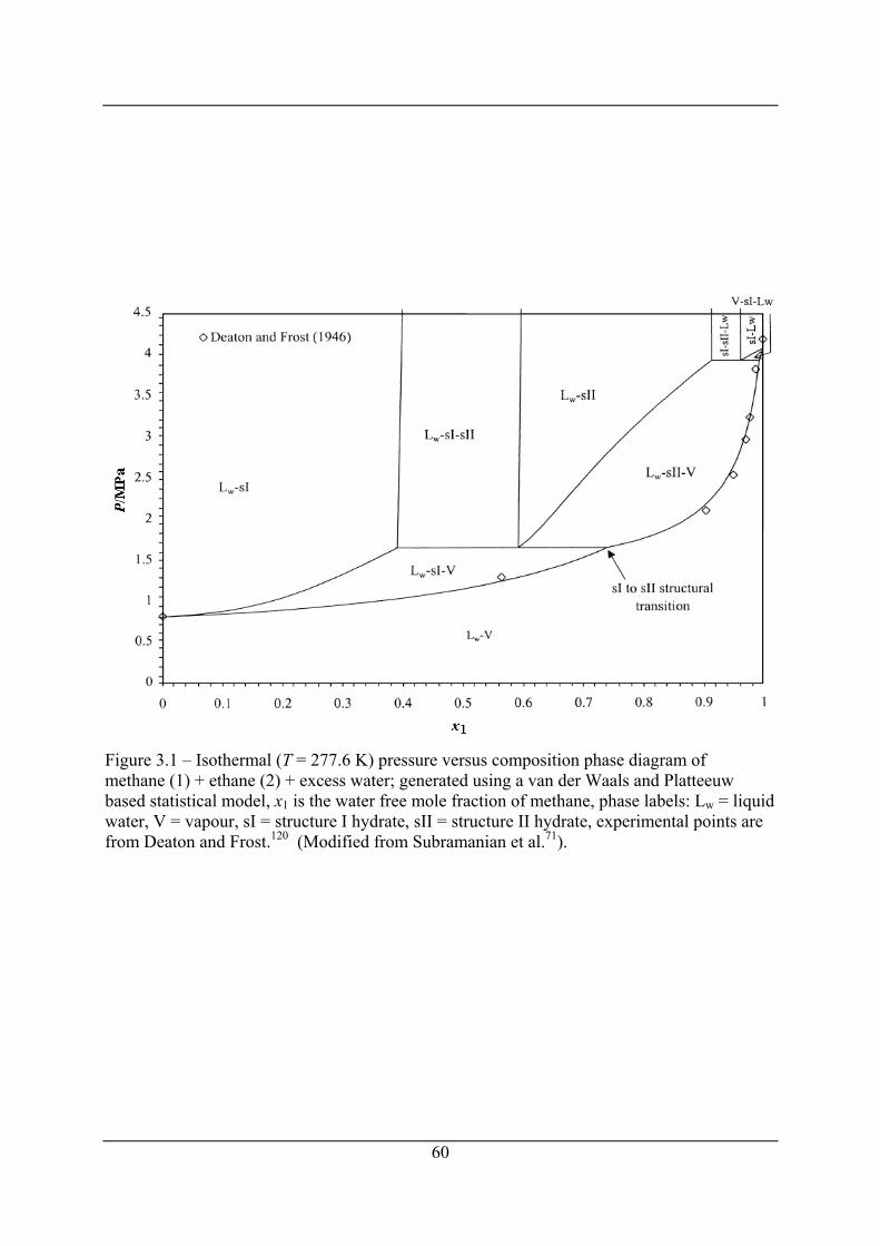
Figure 3.1 – Isothermal (T = 277.6 K) pressure versus composition phase diagram of methane (1) + ethane (2) + excess water; generated using a van der Waals and Platteeuw based statistical model, x1 is the water free mole fraction of methane, phase labels: Lw = liquid water, V = vapour, sI = structure I hydrate, sII = structure II hydrate, experimental points are from Deaton and Frost.120 (Modified from Subramanian et al.71).
60
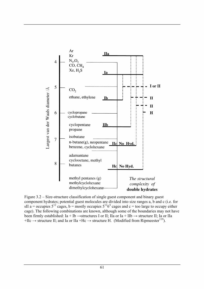
Figure 3.2 – Size-structure classification of single guest component and binary guest component hydrates; potential guest molecules are divided into size ranges a, b and c (i.e. for sII a = occupies 512 cages, b = mostly occupies 51264 cages and c = too large to occupy either cage). The following combinations are known, although some of the boundaries may not have been firmly established: Ia + Ib →structures I or II; IIa or Ia + IIb → structure II; Ia or IIa +IIc → structure II; and Ia or IIa +Hc → structure H. (Modified from Ripmeester119).
61
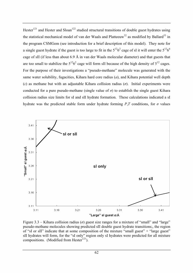
Hester121 and Hester and Sloan122 studied structural transitions of double guest hydrates using
the statistical mechanical model of van der Waals and Platteeuw32 as modified by Ballard33 in
the program CSMGem (see introduction for a brief description of this model). They note for
a single guest hydrate if the guest is too large to fit in the 51262 cage of sI it will enter the 51264
cage of sII (if less than about 6.9 Å in van der Waals molecular diameter) and that guests that
are too small to stabilize the 51262 cage will form sII because of the high density of 512 cages.
For the purpose of their investigations a “pseudo-methane” molecule was generated with the
same water solubility, fugacities, Kihara hard core radius (a), and Kihara potential well depth
(ε) as methane but with an adjustable Kihara collision radius (σ). Initial experiments were
conducted for a pure pseudo-methane (single value of σ) to establish the single guest Kihara
collision radius size limits for sI and sII hydrate formation. These calculations indicated a sI
hydrate was the predicted stable form under hydrate forming P,T conditions, for σ values
Figure 3.3 – Kihara collision radius (σ) guest size ranges for a mixture of “small” and “large” pseudo-methane molecules showing predicted sII double guest hydrate transitions;, the region of “sI or sII” indicate that at some composition of the mixture “small guest” + “large guest” sII hydrates will form, for the “sI only” region only sI hydrates were predicted for all mixture compositions. (Modified from Hester121).
62
63
below 3.11 Å, for σ between (3.11 and 3.43) Å sII was the predicted stable hydrate at hydrate
forming P,T conditions and for σ above 3.43 Å sII was the predicted stable form at hydrate
forming P,T conditions. These calculations provided the size limits for the study of the
double guest hydrates. Double guest hydrates were investigated using two pseudo-methane
molecules with different values of σ, called the “small guest” and “large guest”. The size (σ)
of these pseudo-methane molecules was varied between 3.11 Å and 3.43 Å as well as the
composition of the mixture of “small guest” + “large guest” to reveal the size combination of
“small guest” + “large guest” that could result in a transition to a sII double guest hydrate
(note: this transition may only occur at some compositions of “small guest” + “large guest”,
c.f. Subramanian et al.72 who showed that for methane + ethane mixtures sII will only form at
incipient conditions between a water-free mole fraction of methane of about 0.7 and 0.99). A
plot of this data from Hester121 showing the predicted regions of sI and sI or sII with “large
guest” and “small guest” size (σ) is presented as Figure 3.3. Hester121 also produced a similar
diagram for pseudo-hydrogen sulfide molecules. Hester tested these size limit predictions by
conducting hydrate structural studies in the systems CH4 + C2H4 (confirming the findings of
Sugahara et al.123) and Xe + C2H6 by neutron diffraction and Raman spectroscopy to show
that only sI hydrate would form in these systems.
3.2.2 Structure I to Structure II transitions in hydrates of natural gases Structural transitions of the type that occur in the methane + ethane system also occur in
certain natural gases. A processed natural gas (PNG) is a natural gas composed of mostly
methane, which has had almost all of the heavier and non-combustible components removed.
Bollavaram used a PNG of the composition listed in Table 3.1 to form hydrate plugs.54 In
Chapter 5 of Bollavaram’s thesis entitled “Structural transitions and plug dissociation” (co-
authored with M.D. Jager) P,T conditions for a pipeline flowing this gas were simulated using
OLGA® (note: OLGA® is a software package that performs steady state and transient
simulations of multiphase flows of oil, water and gas in wells, pipelines and receiving
facilities124). Pipeline simulations were completed at start-up conditions (low pressure) and
design conditions (high pressure). A P,T plot of the hydrate formation boundaries as well as
the P,T profiles for the pipeline at design and start-up conditions are shown in Figure 3.4, this
figure was adapted from Bollavaram54 with the hydrate boundaries recalculated in CSMGem
(calculated with a gas to water mole ratio of 100:1, Bollavaram had used Infochem
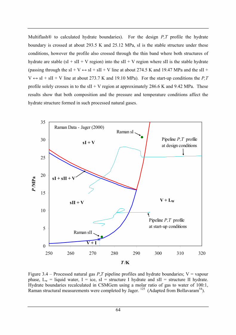
Multiflash® to calculated hydrate boundaries). For the design P,T profile the hydrate
boundary is crossed at about 293.5 K and 25.12 MPa, sI is the stable structure under these
conditions, however the profile also crossed through the thin band where both structures of
hydrate are stable (sI + sII + V region) into the sII + V region where sII is the stable hydrate
(passing through the sI + V ↔ sI + sII + V line at about 274.5 K and 19.47 MPa and the sII +
V ↔ sI + sII + V line at about 273.7 K and 19.10 MPa). For the start-up conditions the P,T
profile solely crosses in to the sII + V region at approximately 286.6 K and 9.42 MPa. These
results show that both composition and the pressure and temperature conditions affect the
hydrate structure formed in such processed natural gases.
0
5
10
15
20
25
30
35
250 260 270 280 290 300 310 320
T /K
P/M
Pa
sII + V
sI + V
V + LW
V + I
sI + sII + V
Pipeline P,T profileat design conditions
Pipeline P,T profileat start-up conditions
Raman sI
Raman sII
Raman Data - Jager (2000)
Figure 3.4 – Processed natural gas P,T pipeline profiles and hydrate boundaries; V = vapour phase, Lw = liquid water, I = ice, sI = structure I hydrate and sII = structure II hydrate. Hydrate boundaries recalculated in CSMGem using a molar ratio of gas to water of 100:1, Raman structural measurements were completed by Jager. 125 (Adapted from Bollavaram54).
64
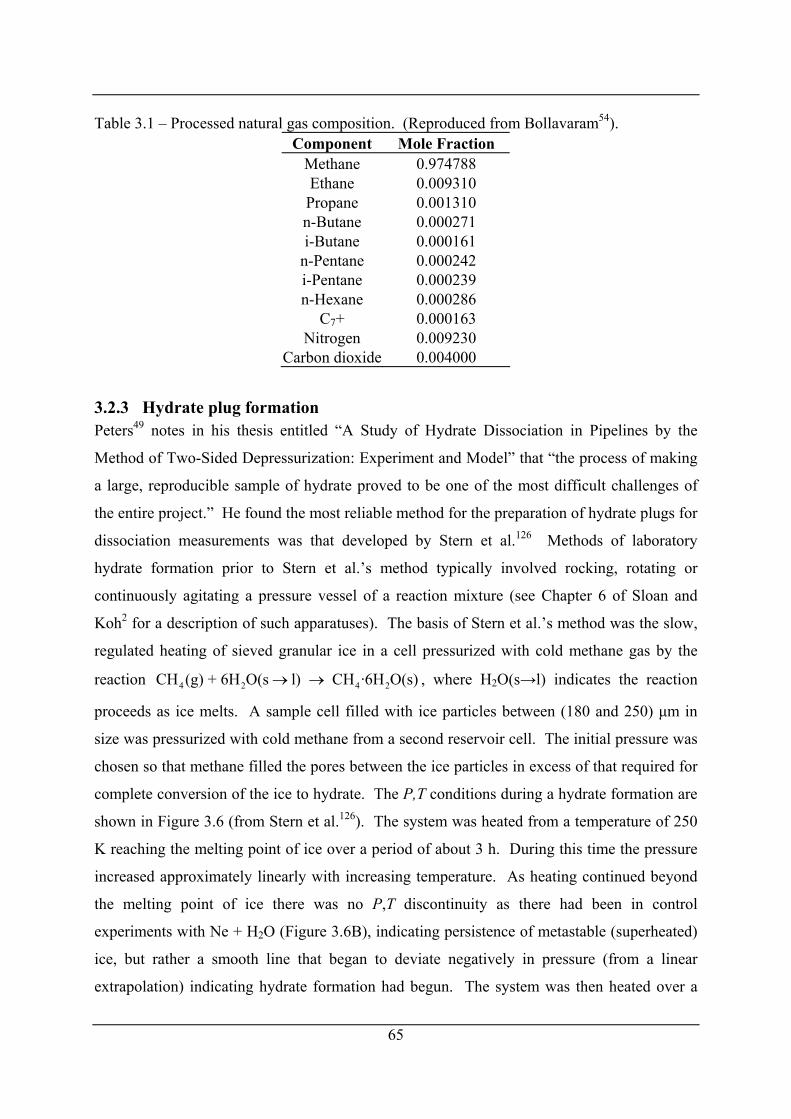
Table 3.1 – Processed natural gas composition. (Reproduced from Bollavaram54). Component Mole Fraction
Methane 0.974788 Ethane 0.009310
Propane 0.001310 n-Butane 0.000271 i-Butane 0.000161
n-Pentane 0.000242 i-Pentane 0.000239 n-Hexane 0.000286
C7+ 0.000163 Nitrogen 0.009230
Carbon dioxide 0.004000
3.2.3 Hydrate plug formation Peters49 notes in his thesis entitled “A Study of Hydrate Dissociation in Pipelines by the
Method of Two-Sided Depressurization: Experiment and Model” that “the process of making
a large, reproducible sample of hydrate proved to be one of the most difficult challenges of
the entire project.” He found the most reliable method for the preparation of hydrate plugs for
dissociation measurements was that developed by Stern et al.126 Methods of laboratory
hydrate formation prior to Stern et al.’s method typically involved rocking, rotating or
continuously agitating a pressure vessel of a reaction mixture (see Chapter 6 of Sloan and
Koh2 for a description of such apparatuses). The basis of Stern et al.’s method was the slow,
regulated heating of sieved granular ice in a cell pressurized with cold methane gas by the
reaction , where H2O(s→l) indicates the reaction
proceeds as ice melts. A sample cell filled with ice particles between (180 and 250) μm in
size was pressurized with cold methane from a second reservoir cell. The initial pressure was
chosen so that methane filled the pores between the ice particles in excess of that required for
complete conversion of the ice to hydrate. The P,T conditions during a hydrate formation are
shown in
4 2 4 2CH (g) + 6H O(s l) CH ·6H O(s)→ →
Figure 3.6 (from Stern et al.126). The system was heated from a temperature of 250
K reaching the melting point of ice over a period of about 3 h. During this time the pressure
increased approximately linearly with increasing temperature. As heating continued beyond
the melting point of ice there was no P,T discontinuity as there had been in control
experiments with Ne + H2O (Figure 3.6B), indicating persistence of metastable (superheated)
ice, but rather a smooth line that began to deviate negatively in pressure (from a linear
extrapolation) indicating hydrate formation had begun. The system was then heated over a
65
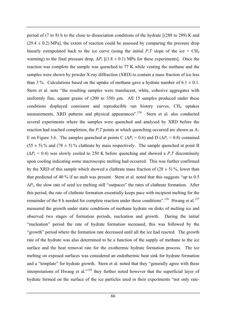
66
period of (7 to 8) h to the close to dissociation conditions of the hydrate [(288 to 289) K and
(29.4 ± 0.2) MPa], the extent of reaction could be assessed by comparing the pressure drop
linearly extrapolated back to the ice curve (using the initial P,T slope of the ice + CH4
warming) to the final pressure drop, ΔPr [(1.8 ± 0.1) MPa for these experiments]. Once the
reaction was complete the sample was quenched to 77 K while venting the methane and the
samples were shown by powder X-ray diffraction (XRD) to contain a mass fraction of ice less
than 3 %. Calculations based on the uptake of methane gave a hydrate number of 6.1 ± 0.1.
Stern et al. note “the resulting samples were translucent, white, cohesive aggregates with
uniformly fine, equant grains of (200 to 350) μm. All 15 samples produced under these
conditions displayed consistent and reproducible run history curves, CH4 uptakes
measurements, XRD patterns and physical appearances”.126 Stern et al. also conducted
several experiments where the samples were quenched and analysed by XRD before the
reaction had reached completion, the P,T points at which quenching occurred are shown as A-
E on Figure 3.6. The samples quenched at points C (ΔPr = 0.6) and D (ΔPr = 0.8) contained
(55 ± 5) % and (78 ± 5) % clathrate by mass respectively. The sample quenched at point B
(ΔPr = 0.4) was slowly cooled to 250 K before quenching and showed a P,T discontinuity
upon cooling indicating some macroscopic melting had occurred. This was further confirmed
by the XRD of this sample which showed a clathrate mass fraction of (28 ± 5) %, lower than
that predicted of 40 % if no melt was present. Stern et al. noted that this suggests “up to 0.5
ΔPr, the slow rate of seed ice melting still “outpaces” the rates of clathrate formation. After
this period, the rate of clathrate formation essentially keeps pace with incipient melting for the
remainder of the 8 h needed for complete reaction under these conditions”.126 Hwang et al.127
measured the growth under static conditions of methane hydrate on disks of melting ice and
observed two stages of formation periods, nucleation and growth. During the initial
“nucleation” period the rate of hydrate formation increased, this was followed by the
“growth” period where the formation rate decreased until all the ice had reacted. The growth
rate of the hydrate was also determined to be a function of the supply of methane to the ice
surface and the heat removal rate for the exothermic hydrate formation process. The ice
melting on exposed surfaces was considered an endothermic heat sink for hydrate formation
and a “template” for hydrate growth. Stern et al. noted that they “generally agree with these
interpretations of Hwang et al.”126 they further noted however that the superficial layer of
hydrate formed on the surface of the ice particles used in their experiments “not only rate-
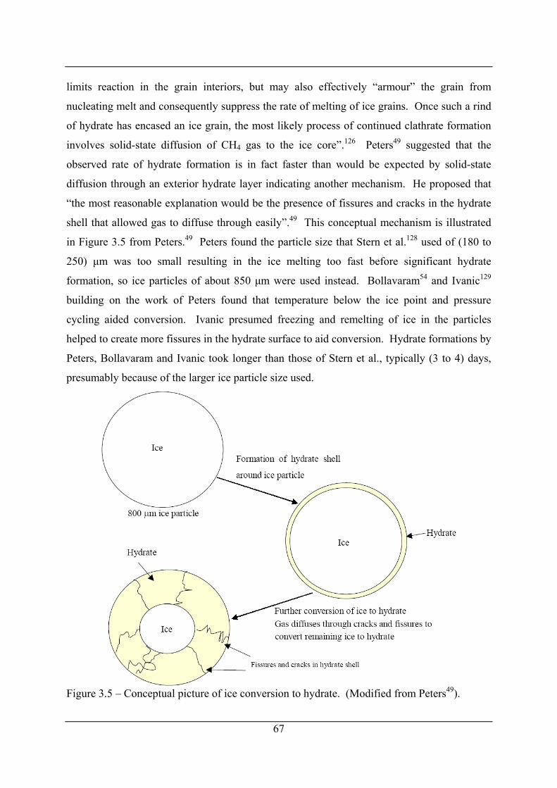
limits reaction in the grain interiors, but may also effectively “armour” the grain from
nucleating melt and consequently suppress the rate of melting of ice grains. Once such a rind
of hydrate has encased an ice grain, the most likely process of continued clathrate formation
involves solid-state diffusion of CH4 gas to the ice core”.126 Peters49 suggested that the
observed rate of hydrate formation is in fact faster than would be expected by solid-state
diffusion through an exterior hydrate layer indicating another mechanism. He proposed that
“the most reasonable explanation would be the presence of fissures and cracks in the hydrate
shell that allowed gas to diffuse through easily”.49 This conceptual mechanism is illustrated
in Figure 3.5 from Peters.49 Peters found the particle size that Stern et al.128 used of (180 to
250) μm was too small resulting in the ice melting too fast before significant hydrate
formation, so ice particles of about 850 μm were used instead. Bollavaram54 and Ivanic129
building on the work of Peters found that temperature below the ice point and pressure
cycling aided conversion. Ivanic presumed freezing and remelting of ice in the particles
helped to create more fissures in the hydrate surface to aid conversion. Hydrate formations by
Peters, Bollavaram and Ivanic took longer than those of Stern et al., typically (3 to 4) days,
presumably because of the larger ice particle size used.
Figure 3.5 – Conceptual picture of ice conversion to hydrate. (Modified from Peters49).
67
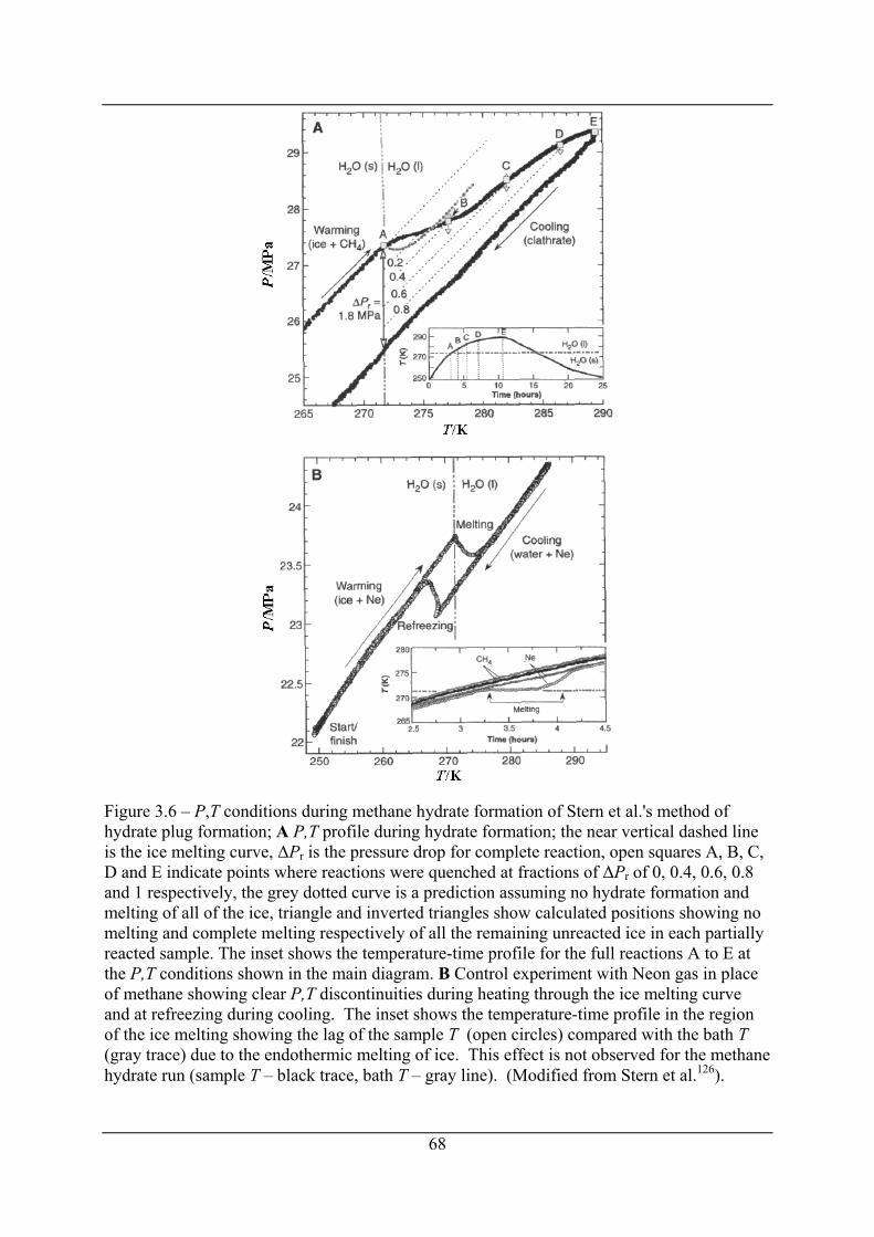
Figure 3.6 – P,T conditions during methane hydrate formation of Stern et al.'s method of hydrate plug formation; A P,T profile during hydrate formation; the near vertical dashed line is the ice melting curve, ΔPr is the pressure drop for complete reaction, open squares A, B, C, D and E indicate points where reactions were quenched at fractions of ΔPr of 0, 0.4, 0.6, 0.8 and 1 respectively, the grey dotted curve is a prediction assuming no hydrate formation and melting of all of the ice, triangle and inverted triangles show calculated positions showing no melting and complete melting respectively of all the remaining unreacted ice in each partially reacted sample. The inset shows the temperature-time profile for the full reactions A to E at the P,T conditions shown in the main diagram. B Control experiment with Neon gas in place of methane showing clear P,T discontinuities during heating through the ice melting curve and at refreezing during cooling. The inset shows the temperature-time profile in the region of the ice melting showing the lag of the sample T (open circles) compared with the bath T (gray trace) due to the endothermic melting of ice. This effect is not observed for the methane hydrate run (sample T – black trace, bath T – gray line). (Modified from Stern et al.126).
68
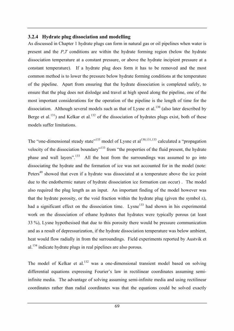
69
3.2.4 Hydrate plug dissociation and modelling As discussed in Chapter 1 hydrate plugs can form in natural gas or oil pipelines when water is
present and the P,T conditions are within the hydrate forming region (below the hydrate
dissociation temperature at a constant pressure, or above the hydrate incipient pressure at a
constant temperature). If a hydrate plug does form it has to be removed and the most
common method is to lower the pressure below hydrate forming conditions at the temperature
of the pipeline. Apart from ensuring that the hydrate dissociation is completed safely, to
ensure that the plug does not dislodge and travel at high speed along the pipeline, one of the
most important considerations for the operation of the pipeline is the length of time for the
dissociation. Although several models such as that of Lysne et al.130 (also later described by
Berge et al.131) and Kelkar et al.132 of the dissociation of hydrates plugs exist, both of these
models suffer limitations.
The “one-dimensional steady state”133 model of Lysne et al130,131,133 calculated a “propagation
velocity of the dissociation boundary”133 from “the properties of the fluid present, the hydrate
phase and wall layers”.133 All the heat from the surroundings was assumed to go into
dissociating the hydrate and the formation of ice was not accounted for in the model (note:
Peters49 showed that even if a hydrate was dissociated at a temperature above the ice point
due to the endothermic nature of hydrate dissociation ice formation can occur) . The model
also required the plug length as an input. An important finding of the model however was
that the hydrate porosity, or the void fraction within the hydrate plug (given the symbol ε),
had a significant effect on the dissociation time. Lysne133 had shown in his experimental
work on the dissociation of ethane hydrates that hydrates were typically porous (at least
33 %), Lysne hypothesised that due to this porosity there would be pressure communication
and as a result of depressurization, if the hydrate dissociation temperature was below ambient,
heat would flow radially in from the surroundings. Field experiments reported by Austvik et
al.134 indicate hydrate plugs in real pipelines are also porous.
The model of Kelkar et al.132 was a one-dimensional transient model based on solving
differential equations expressing Fourier’s law in rectilinear coordinates assuming semi-
infinite media. The advantage of solving assuming semi-infinite media and using rectilinear
coordinates rather than radial coordinates was that the equations could be solved exactly
70
rather than by numerical solution. The dissociation was assumed to be by rapid
depressurization and modelled by either a single or double Stefan moving boundary. If the
ambient temperature was below 0 °C then only two phases were present, ice and hydrate, with
only a single moving boundary. However if the ambient temperature was above the 0 °C but
the hydrate dissociation temperature at the pressure selected for dissociation was below 0 °C
then three phases were considered present, hydrate, ice and water, resulting in a double
moving boundary problem. If the hydrate dissociation temperature at the selected pressure
was above 0 °C then only hydrate and water were considered resulting in a single moving
boundary. An interesting finding by Kelkar et al.132 was that due to the high thermal
diffusivity, ice aided the rate of dissociation of the hydrate.
Peters49 model of the two-sided dissociation of hydrate plugs was similar to that of Kelkar et
al.132 except it was expressed and solved in radial coordinates. The model has the following
assumptions:
• The hydrate is dissociated due to a step change in pressure on both sides of the plug to
a pressure below the hydrate dissociation pressure at the ambient temperature,
• Hydrate and ice are both porous,
• The hydrate dissociation temperature is uniform,
• Radial dissociation dominates over axial dissociation,
• Dissociation is heat transfer controlled and
• Only heat conduction is important.
Solving the equations for radial coordinates required a numerical solution, details of which
are not included here (see Peter’s thesis49 for details). The problem could either be a single or
double Stefan moving boundary problem, the same as Kelkar et al.’s model. Figure 3.7
shows the phases and temperature gradients for the three phase (hydrate, ice and water) two
moving boundary problem. The temperature profiles for this system, with constant wall
temperature, according to Fourier’s law of heat conduction in radial coordinates are described
for t >0 (where t is time) by eqs (3.1) to (3.7), where r0, rF1 and rF2 are the radius of the wall,
moving boundary between water and ice and moving boundary between the ice and hydrate
respectively, T0 TW, TI, TD and TM are the wall, water, ice, hydrate dissociation and ice
melting point temperatures, αW and αI are thermal diffusivity of the water and ice, ρW and ρI
are the density of ice and water, kW and kI are the thermal conductivity of water and ice, λH
and λI are the enthalpy of hydrate dissociation and enthalpy of fusion of ice and ε is the
porosity of the hydrate respectively.
For : F1 0r r r< <
2
W WW 2
1T Tt r r r
α⎛ ⎞∂ ∂ ∂
= +⎜∂ ∂⎝ ⎠WT⎟∂
. (3.1)
For : F2 F1r r r< <
2
I II 2
1T Tt r r r
α⎛ ⎞∂ ∂ ∂
= +⎜∂ ∂ ∂⎝ ⎠IT⎟
0
. (3.2)
Eqs (3.1) and (3.2) are subject to the boundary conditions: at : 0 r r=
WT T= , (3.3)
at : F1r r=
( )W IW I I I
d1d
T Tk kr r
ε ρ λ∂ ∂− = − + −
∂ ∂F1rt
M
, (3.4)
and
W IT T T= = , (3.5)
at : F2r r=
( )II H
d1d
Tkr t
ε ρ λ F2H
r∂− = −
∂, (3.6)
and
IT TD= . (3.7)
The boundary conditions of eqs (3.3), (3.5) and (3.7) are due to the pipe wall, water-ice
moving boundary and the ice-hydrate moving boundary respectively. Equations (3.4) and
(3.6) are heat flow boundary conditions. Equation (3.4) expresses that the heat conducted
through the water layer is equal to the heat conducted through the ice layer minus the heat
71
used to melt the ice to water, whereas eq (3.6) express that the heat conducted though the ice
layer is utilised to dissociate the hydrate.
The model solves for the time when the hydrate plug has completely dissociated (time when
rF2 = 0, or when the ice-hydrate moving boundary reaches the centre of the pipe) as well as
the time when an ice plug if present is completely melted (time when rF1 = 0, or when the ice-
water moving boundary reached the centre of the pipe).
Figure 3.7 – Radial two-sided dissociation of hydrate plug for a double moving boundary including hydrate, ice and water phases. (Modified from Peters49).
72
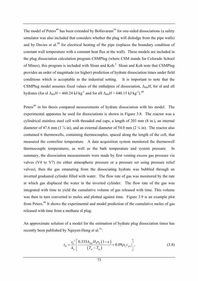
The model of Peters49 has been extended by Bollavaram54 for one-sided dissociations (a safety
simulator was also included that considers whether the plug will dislodge from the pipe walls)
and by Davies et al.40 for electrical heating of the pipe (replaces the boundary condition of
constant wall temperature with a constant heat flux at the wall). These models are included in
the plug dissociation calculation program CSMPlug (where CSM stands for Colorado School
of Mines), this program is included with Sloan and Koh.2 Sloan and Koh note that CSMPlug
provides an order of magnitude (or higher) prediction of hydrate dissociation times under field
conditions which is acceptable to the industrial setting. It is important to note that the
CSMPlug model assumes fixed values of the enthalpies of dissociation, ΔdisH, for sI and sII
hydrates (for sI ΔdisH = 460.24 kJ·kg-1 and for sII ΔdisH = 640.15 kJ·kg-1).40
Peters49 in his thesis compared measurements of hydrate dissociation with his model. The
experimental apparatus he used for dissociations is shown in Figure 3.8. The reactor was a
cylindrical stainless steel cell with threaded end caps, a length of 203 mm (8 in.), an internal
diameter of 47.6 mm (1 ⅞ in), and an external diameter of 54.0 mm (2 ⅛ in). The reactor also
contained 6 thermowells, containing thermocouples, spaced along the length of the cell, that
measured the centreline temperature. A data acquisition system monitored the thermowell
thermocouple temperatures, as well as the bath temperature and system pressure. In
summary, the dissociation measurements were made by first venting excess gas pressure via
valves (V4 to V7) (to either atmospheric pressure or a pressure set using pressure relief
valves), then the gas emanating from the dissociating hydrate was bubbled through an
inverted graduated cylinder filled with water. The flow rate of gas was monitored by the rate
at which gas displaced the water in the inverted cylinder. The flow rate of the gas was
integrated with time to yield the cumulative volume of gas released with time. This volume
was then in turn converted to moles and plotted against time. Figure 3.9 is an example plot
from Peters.49 It shows the experimental and model prediction of the cumulative moles of gas
released with time from a methane sI plug.
An approximate solution of a model for the estimation of hydrate plug dissociation times has
recently been published by Nguyen-Hong et al.51:
( )( )
2dis H0
DL w m
0.335 10.09 p
Hrtk T T
ρ ερ
⎡ ⎤Δ −= +⎢ −⎣ ⎦
L Lc ⎥ , (3.8)
73
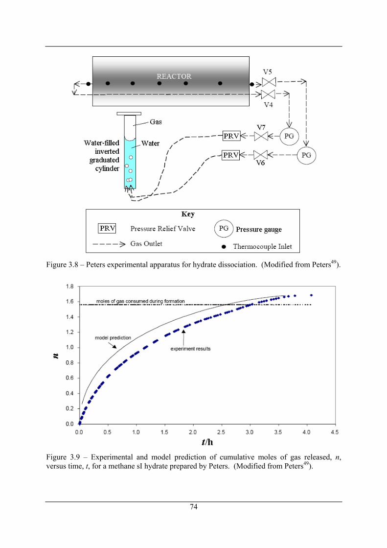
Figure 3.8 – Peters experimental apparatus for hydrate dissociation. (Modified from Peters49).
Figure 3.9 – Experimental and model prediction of cumulative moles of gas released, n, versus time, t, for a methane sI hydrate prepared by Peters. (Modified from Peters49).
74
where the tD is the dissociation time, r0 is the internal radius of the pipeline, k is the thermal
conductivity, ΔdisH is the enthalpy of dissociation of the hydrate, ρ is the density, ε is the plug
porosity (void fraction that can be occupied by gas), TW the internal pipe wall temperature, Tm
is the dissociation temperature of the hydrate and cp is the specific heat capacity, the
subscripts L and H refer to the liquid and hydrate phase respectively. The model assumes the
depressurisation of the plug is slow so that no ice is formed. The model was shown to be
valid for plug porosities between 0.3 and 0.9 with an average error of about 4 % for
dissociation temperatures (Tm) between 273.15 K and 277.15 K.
3.2.5 Enthalpies of dissociation of gas hydrates The dissociation of a gas hydrate is described by eqs (3.9) and (3.10). Generally if the
dissociation conditions are above the ice point (on the liquid side of the water melting line)
the hydrate will dissociate in to gas and aqueous phases (eq (3.9)) whereas if the dissociation
conditions are below the ice point the hydrate will dissociate in to gas and ice phases. For a
single guest hydrate dissociated above the ice point under idealised conditions where the guest
is considered insoluble in water and no water is present in the vapour phase then eq (3.11)
describes the stoichiometry of the dissociation, similarly eq (3.12) describes the dissociation
below the ice point. In these equations G represents the guest molecule (for example CH4)
and n represent the hydrate number or the number of moles of water per mole of guest in the
hydrate.
(3.9) Hydrate Aqueous Solution + Vapour→
(3.10) Hydrate Ice + Vapour→
( )2G· H O(s) G g H O(l)n → + 2n (3.11)
( )2G· H O(s) G g H O(s)n → + 2n (3.12)
The enthalpy of dissociation is the amount of energy at constant pressure required to
dissociate the hydrate by either of the reactions given by eqs. (3.9) or (3.10). This enthalpy
75
76
may be experimentally measured by calorimetry or may be calculated from P,T phase data
using the Clapeyron equation.2
The enthalpy of many natural gas components have been measured by calorimetry as well as
several mixtures. Values of the enthalpies of dissociation for single guest component
hydrates are listed in Table 3.2. Handa at the National Research Council of Canada measured
dissociation enthalpies for several single guest hydrates of natural gas components namely
methane, ethane, propane and isobutane using a Tian-Calvet heat flow calorimeter at low
temperatures.135 Samples of hydrate were prepared outside of the calorimeter from powdered
ice and gas in a rolling rod mill and stored in liquid nitrogen until use. The hydrates were
loaded in to a sample calorimeter cell that was cooled in a liquid nitrogen bath, in turn the cell
was loaded into the calorimeter that was precooled to 78 K. Enthalpies of dissociation were
measured at temperatures between (160 and 210) K for methane, (190 to 250) K for ethane,
(210 to 260) K for propane and (230 to 260) K for isobutane. The temperature at which
dissociation occurred was varied by adjusting the pressure of the gas in the calorimeter cell.
Heat capacities of the methane, ethane and propane hydrates were also measured between (85
and 270) K (note: 260 K was the maximum measurement temperature for the ethane and
propane hydrates). Handa presented a method of calculating the hydrate dissociation enthalpy
at standard P,T conditions of 0.1013 MPa and 273.15 K.136 He used this method to calculate
the enthalpies of dissociation of hydrate at both the H+I+V (hydrate + ice + vapour) and
H+LW+V (hydrate + aqueous solution + vapour) points at these standard conditions for the
methane, ethane and propane hydrate. Handa also presented measurements for two naturally
occurring hydrates, a sI sample from the Mid America Trench off Guatemala and a sII sample
from the Green Canyon area of the northern Gulf of Mexico.137
Several other authors have also reported calorimetric measurements of enthalpies of
dissociation. Lievois et al.138 published measurements of the enthalpy of dissociation of
methane hydrate at 278.15 K and 283.15 K using a pressurised heat flux Calvet calorimeter.
Isothermal dissociation measurements were taken at nearly constant pressure by slowly
expanding the available volume using a high pressure pump. Rueff et al.139 measured the
enthalpy of dissociation of methane hydrate by differential scanning calorimetry (Perkins-
Elmer DSC-2) at 285 K. Rueff et al. also lists measurements of the enthalpy of dissociation
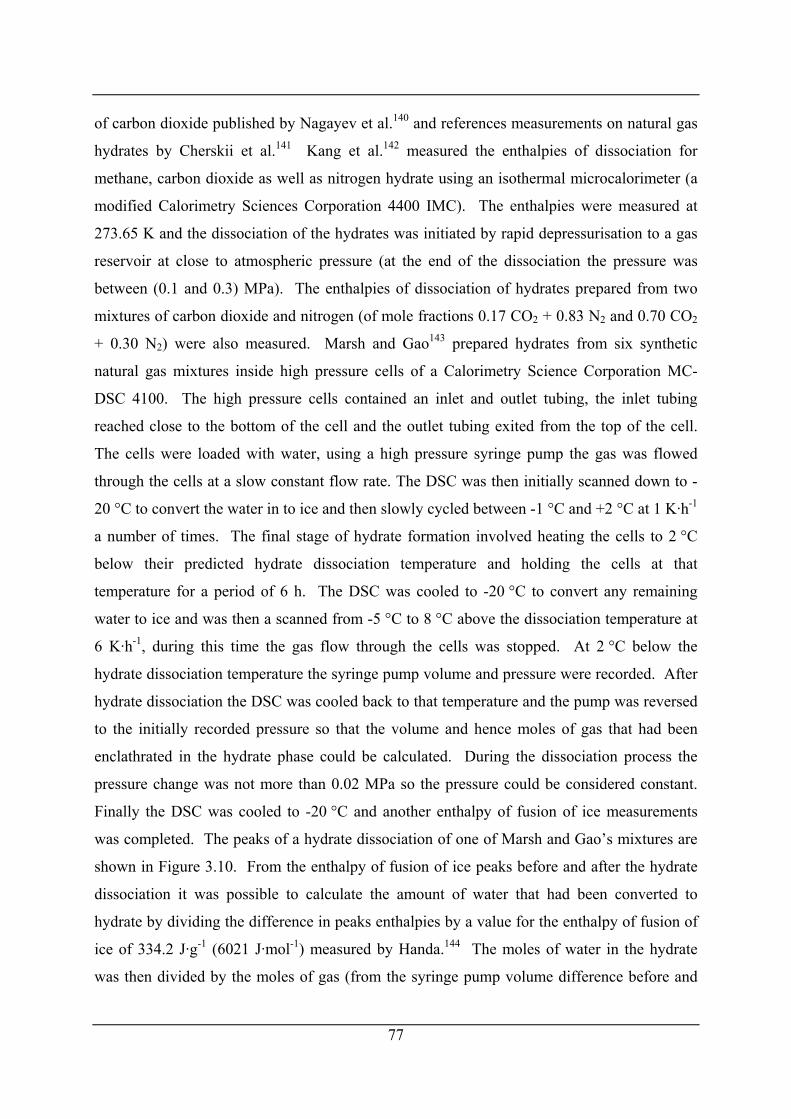
77
of carbon dioxide published by Nagayev et al.140 and references measurements on natural gas
hydrates by Cherskii et al.141 Kang et al.142 measured the enthalpies of dissociation for
methane, carbon dioxide as well as nitrogen hydrate using an isothermal microcalorimeter (a
modified Calorimetry Sciences Corporation 4400 IMC). The enthalpies were measured at
273.65 K and the dissociation of the hydrates was initiated by rapid depressurisation to a gas
reservoir at close to atmospheric pressure (at the end of the dissociation the pressure was
between (0.1 and 0.3) MPa). The enthalpies of dissociation of hydrates prepared from two
mixtures of carbon dioxide and nitrogen (of mole fractions 0.17 CO2 + 0.83 N2 and 0.70 CO2
+ 0.30 N2) were also measured. Marsh and Gao143 prepared hydrates from six synthetic
natural gas mixtures inside high pressure cells of a Calorimetry Science Corporation MC-
DSC 4100. The high pressure cells contained an inlet and outlet tubing, the inlet tubing
reached close to the bottom of the cell and the outlet tubing exited from the top of the cell.
The cells were loaded with water, using a high pressure syringe pump the gas was flowed
through the cells at a slow constant flow rate. The DSC was then initially scanned down to -
20 °C to convert the water in to ice and then slowly cycled between -1 °C and +2 °C at 1 K·h-1
a number of times. The final stage of hydrate formation involved heating the cells to 2 °C
below their predicted hydrate dissociation temperature and holding the cells at that
temperature for a period of 6 h. The DSC was cooled to -20 °C to convert any remaining
water to ice and was then a scanned from -5 °C to 8 °C above the dissociation temperature at
6 K·h-1, during this time the gas flow through the cells was stopped. At 2 °C below the
hydrate dissociation temperature the syringe pump volume and pressure were recorded. After
hydrate dissociation the DSC was cooled back to that temperature and the pump was reversed
to the initially recorded pressure so that the volume and hence moles of gas that had been
enclathrated in the hydrate phase could be calculated. During the dissociation process the
pressure change was not more than 0.02 MPa so the pressure could be considered constant.
Finally the DSC was cooled to -20 °C and another enthalpy of fusion of ice measurements
was completed. The peaks of a hydrate dissociation of one of Marsh and Gao’s mixtures are
shown in Figure 3.10. From the enthalpy of fusion of ice peaks before and after the hydrate
dissociation it was possible to calculate the amount of water that had been converted to
hydrate by dividing the difference in peaks enthalpies by a value for the enthalpy of fusion of
ice of 334.2 J·g-1 (6021 J·mol-1) measured by Handa.144 The moles of water in the hydrate
was then divided by the moles of gas (from the syringe pump volume difference before and
after hydrate dissociation) to give the hydrate number, n. The enthalpy of hydrate
dissociation could then be calculated from the dissociation peak.
Figure 3.10 – Calorimetric response for enthalpy measurements Marsh and Gao’s mixture 3 at 2.07 MPa. (Reproduced from Marsh and Gao.143).
Levik145 made enthalpy of dissociation measurements on hydrate prepared in a laboratory
scale flow loop from a mixture containing mole fractions of 92 % methane + 5 % ethane + 3%
propane. Measurements were completed in a pressurizable Setaram BT2.15 heat flow
calorimeter.
Gupta50 measured the enthalpies of dissociation of methane hydrate at temperatures between
280.60 K and 291.65 K using a High Pressure Setaram Micro-Differential Scanning
Calorimeter VIIa. Hydrate samples were prepared from powdered ice using a method similar
to Stern et al.126 and transferred cryogenically with liquid nitrogen at atmospheric pressure to
the DSC sample cell. Heat capacities of the hydrate were also measured.
Rydzy et al.146 completed measurements of the enthalpies of dissociation of hydrates prepared
from pure methane and four different mixtures, two containing methane + carbon dioxide and
two containing methane + ethane + propane. Hydrates were prepared in a high pressure cell
78
79
from gas and powdered ice. The calorimeter used was a Setaram Calvet DSC 121 that could
be cooled with liquid nitrogen. Measurements on the dissociation of hydrates were completed
at atmospheric pressure hence the dissociation points were at low temperatures below 273 K
and the hydrate dissociated to ice + gas. Interestingly a mixture of mole fractions 98 %
methane + 1 % ethane + 1 % propane was demonstrated to have formed a mixture of sI and
sII hydrates by both calorimetry (two separate hydrate dissociation peaks were observed) and
powder X-ray diffraction.
Table 3.2 – Calorimetric measurements of enthalpies of dissociation for single guest hydrates of natural gas components. Guest T/K P/MPa n ΔdisH/kJ·mol-1 Reference CH4 H+I+V 273.15 0.101325 6 18.13a ± 0.27 Handa135
H+Aq+V 273.15 0.101325 6 54.19a ± 0.28 Handa135 H+Aq+V 285b c 6.04d 54.63e ± 0.79 Rueff et al.139 H+Aq+V 278.15 4.217 5.97 57.65 ± 1.50 Lievois et al.138 H+Aq+V 283.15 7.110 5.98 53.24 ± 1.38 Lievois et al.138 H+Aq+V 273.65 0.1 to 0.3 6.38 56.84 ± 0.89 Kang et al.142 H+Aq+V 280.6 to
292.16 5.5 to 19.3
6 54.44b ± 1.45 Gupta50
C2H6 H+I+V 273.15 0.101325 7.67 25.70a ± 0.37 Handa135 H+Aq+V 273.15 0.101325 7.67 71.80a ± 0.38 Handa135
C3H8 H+I+V 273.15 0.101325 17.0 27.00a ± 0.33 Handa135 H+Aq+V 273.15 0.101325 17.0 129.2a ± 0.4 Handa135
iC4H10 H+I+V 273.15 0.101325 17.0 31.07a ± 0.20 Handa135 H+Aq+V 273.15 0.101325 17.0 133.2a ± 0.3 Handa135
CO2 H+Aq+V 279 c 6.00f 51.02e,g Nagayev et al.140 h H+Aq+V 281 c 5.82f 56.88e,g Nagayev et al.140 h H+Aq+V 273.65 0.1 to 0.3 7.23 65.22 ± 1.03 Kang et al.142
N2 H+Aq+V 273.65 0.1 to 0.3 5.94 65.81 ± 1.04 Kang et al.142 a Calculated at standard state of 273.15 K and 0.101325 MPa, see Handa135 for details, H+Aq+V values calculated used the enthalpy of fusion of ice at 273.15 K. b Averaged value for all measurements. c Not measured or unknown. d Estimated from CSMGem at 285 K. e Calculated from mass specific enthalpy of dissociation. f Estimated from Anderson.147 g Uncertainty unknown. h Values were listed in Rueff et al.139
The calorimetrically measured enthalpies of dissociation for single guest hydrates of natural
gas components are listed in Table 3.2. The H+Aq+V enthalpies of dissociation for methane
hydrate of Handa,135 Rueff et al.,139 Lievois et al.138 at 283.15 K, and Gupta agree within error
despite being measured at different P,T conditions. The values of Lievois et al.138 at 278.15
K and Kang et al.142 are approximately 3 kJ·mol-1 higher than the other measurements. The
only other single component for which measurements have been conducted by more than one
group is that for carbon dioxide. The enthalpies of dissociation of CO2 hydrate by Nagayev et
al.140 (listed in Rueff et al.139) are considerably lower than the measurement by Kang et al.142
More measurements are needed on system to confirm the value of the enthalpies of
dissociation of CO2 hydrate.
The Clapeyron equation is typically used to calculate the enthalpy of vaporisation from
vapour pressure data of a pure component. It expresses the enthalpy of vaporisation, ΔvapH, in
terms of the temperature, the change in volume, ΔV, and the vapour pressure P,T slope,
dP/dT:
vapdd
PH T VT
Δ = Δ . (3.13)
As Van der Waals and Platteuw148 point out the Clapeyron equation “is a direct consequence
of the second law of thermodynamics, and as such exact for all univariant equilibria,
irrespective of the number of components”. As a consequence of this they considered a
binary hydrate forming system of water + gas. The points of three phase equilibria along
either the H+I+V or H+LW+V line of such a system are “univariant ones in which the
composition of the clathrate varies along the three phase lines”. Barrer notes that care should
be taken due to the non-stoichiometry of hydrates (n, the hydrate number varies with the P,T
conditions), and notes that n should be determined at the same time as the enthalpy of
dissociation to ensure that the values does not have “uncertain meaning”.149 Glew suggested
that while there are deviations of n from the ideal value required to fill all the cages that
generally n varies very little along the hydrate formation lines except for molecules that are
approaching the upper limit of the cavity sizes such as ethane, methyl bromide and bromine in
sI.150 Glew also suggested that making all the corrections such as allowing for “phase volume
changes, gas imperfections, gas solubility and water saturations” was very important and
should be made when “hydrate saturation pressures greater than one atmosphere are involved
for example, for argon and methane hydrates”.
80
An alternative expression of the Clapeyron equation can be derived from eq (3.13) if a
compressibility factor difference, ΔZ, is defined in terms of the volume change:
P VZRTΔ
Δ = , (3.14)
and the mathematical relationships d d lnP P P= and ( )2d d 1T T T= − are applied:
( )vap
d lnd 1
PH R ZT
Δ = − Δ , (3.15)
If the Clapeyron equation is applied for the enthalpy of hydrate dissociation is
replaced by . The advantage of this form of the Clapeyron equation is that plots of lnP
versus 1/T yield linear relationships (constant value of dlnP/d[1/T]) over larger P,T ranges
than plots of P versus T. Assuming limited solubility of the vapour in the water and limited
vaporisation of water in to the vapour phase (i.e. after dissociation of the hydrate the aqueous
phase contains no molecules of the hydrate guest so is pure water and the vapour phase
contains no water so the vapour phase is pure guest) ΔV can be calculated by:
vapHΔ
disHΔ
, (3.16) 2G H OV V nV VΔ = + − H
H
where VH is the molar volume of the hydrate (defining one mole of hydrate as M·nH2O, i.e.
one mole of hydrate has a molar mass that is the sum of the molar mass of M and the molar
mass of n water molecules), VG is the molar volume of the gaseous hydrate guest phase, and
2H OV is the molar volume of the water phase (ice or liquid water). The compressibility factor
difference can then be similarly defined as:
2G H OZ Z nZ ZΔ = + − , (3.17)
81
by multiplying eq (3.16) by P/(RT). Roberts et al.151, Barrer and Edge152 and Skovborg and
Rasmussen153 present similar forms of the Clapeyron equation where the solubility of the
guest in the aqueous phase and water content of the vapour are taken in to account, Barrer and
Edge also consider a double hydrate composed of a water insoluble liquid guest (CHCl3) and
a gaseous guest. Skovborg and Rasmussen note that CO2 and H2S have a “somewhat higher
solubility” in water than most gas hydrate guest components suggesting it may not be
appropriate to make assumption of no solubility of the guest in the aqueous phase.
Sloan and Fleyfel154 calculated the enthalpies of dissociation for methane, ethane, propane
and isobutane hydrates assuming that GZ ZΔ = (or GV VΔ = ), from experimental LW-H-V P,T
data (note: when this form is used the Clapeyron equation is referred to as the Clausius-
Clapeyron equation). Sloan and Fleyfel154 compared their calculated values with the
calorimetric data of Handa136, these values are listed in Table 3.3, and show close agreement
(the calculated values deviate between (1 and 5)% from the calorimetric measurements).
Sloan and Fleyfel154 further suggested that to a first approximation for a sI or sII hydrate the
size of the guest molecule fixes the enthalpy of dissociation, as the size of the molecule
determines which cages are occupied. The initial paper of Sloan and Fleyfel was commented
on in a letter to the editor of the journal “Fluid Phase Equilibria” by Skovborg and
Rasmussen153 who critiqued the paper and suggested that Sloan and Fleyfel154 were incorrect.
They deducted a hypothetical empty lattice hydrate dissociation value from Sloan and
Fleyfel’s enthalpies to magnify the differences in enthalpies of dissociation in terms of the
guest molecules contribution and suggested the relationship broke down from their results.
However Sloan and Fleyfel155 noted in a reply to the comments “we concur with their
conclusion, but suggest that to ignore “the different amounts of water in the hydrate” would
be to ignore the largest portion of the heat of dissociation, i.e. that due to hydrogen bonding”
and that Skovborg and Rasmussen’s mathematical derivation of hydrate dissociation
“suggests a limit to our engineering approximation to explain these phenomena”. They also
produced a plot to show the slope, dlnP/d(1/T), as a function of the size of the hydrate guest,
shown in Figure 3.11, to emphasize the relationship between the cavity size and the
dissociation enthalpy. It was also noted from lnP versus 1/T plots for hydrates of binary gas
mixtures of the same components but with different compositions that the data for each
82
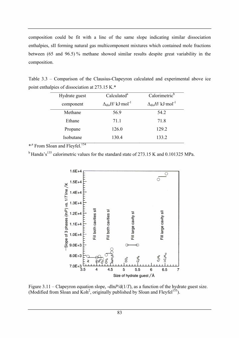
composition could be fit with a line of the same slope indicating similar dissociation
enthalpies, sII forming natural gas multicomponent mixtures which contained mole fractions
between (65 and 96.5) % methane showed similar results despite great variability in the
composition.
Table 3.3 – Comparison of the Clausius-Clapeyron calculated and experimental above ice
point enthalpies of dissociation at 273.15 K.*
Hydrate guest
component
Calculateda
ΔdisH/ kJ·mol-1
Calorimetricb
ΔdisH/ kJ·mol-1
Methane 56.9 54.2
Ethane 71.1 71.8
Propane 126.0 129.2
Isobutane 130.4 133.2
*,a From Sloan and Fleyfel.154 b Handa’s135 calorimetric values for the standard state of 273.15 K and 0.101325 MPa.
Figure 3.11 – Clapeyron equation slope, -dlnP/d(1/T), as a function of the hydrate guest size. (Modified from Sloan and Koh2, originally published by Sloan and Fleyfel155).
83
Recently several papers have been published that attempt to obtain more accurate values of
the enthalpy of dissociation of gas hydrates using the Clapeyron equations. Anderson147
regressed seven sets of carbon dioxide H+Aq+V data to generate a polynomial equation for
dP/dT for use in the eq (3.13) form of the Clapeyron equation. A volume difference equation
was developed which took into account the solubility of CO2 in water and the volume of the
hydrate phase:
2
2
COAq
V AqCOAq
11nx
V V nVx
⎛ ⎞Δ = − + −⎜ ⎟⎜ ⎟−⎝ ⎠
HV , (3.18)
where 2COAqx is the mole fraction of CO2 in the aqueous phase (see Appendix D for a
discussion of the stoichiometry of hydrate dissociation). This equation accounts for the
reduction in volume of the vapour phase due to the high solubility of CO2 in water. The
vapour phase molar volume was considered to be pure CO2 (no water), the aqueous volume
was calculated from the molar volume of pure water and the infinite dilution partial molar
volume of CO2 in water, and the hydrate molar volume was calculated from a X-ray
diffraction calculated CO2 hydrate density. Anderson defined dissociation enthalpies based
on two equations for above the ice point hydrate dissociations, these were:
( ) ( ) ( )2 2 2 2CO · H O s CO g H O ln → + n , (3.19)
and
( ) ( ) ( )2
2
COAq
2 2 2 2 2COAq
CO · H O s 1 CO g H O l,CO sat1nx
n nx
⎛ ⎞→ − +⎜ ⎟⎜ ⎟−⎝ ⎠
. (3.20)
As eq (3.19) was referred to as reaction I in Anderson paper the enthalpy of dissociation for
this reaction was referred to as ΔHI, similarly eq (3.20) was referred to as reaction IV and is
the enthalpy of dissociation for this reaction was referred to as ΔHIV. The connection between
these two equations is:
( ) ( ) ( )2
2
COAq
2 2 2 2COAq
H O l,CO sat H O l CO g1nx
n nx
⎛ ⎞→ + ⎜ ⎟⎜ ⎟−⎝ ⎠
, (3.21)
84
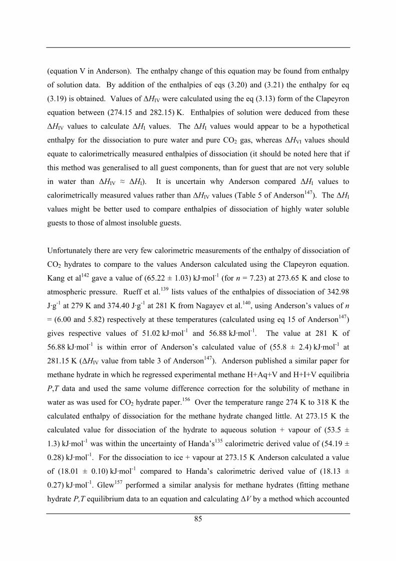
85
(equation V in Anderson). The enthalpy change of this equation may be found from enthalpy
of solution data. By addition of the enthalpies of eqs (3.20) and (3.21) the enthalpy for eq
(3.19) is obtained. Values of ΔHIV were calculated using the eq (3.13) form of the Clapeyron
equation between (274.15 and 282.15) K. Enthalpies of solution were deduced from these
ΔHIV values to calculate ΔHI values. The ΔHI values would appear to be a hypothetical
enthalpy for the dissociation to pure water and pure CO2 gas, whereas ΔHVI values should
equate to calorimetrically measured enthalpies of dissociation (it should be noted here that if
this method was generalised to all guest components, than for guest that are not very soluble
in water than ΔHIV ≈ ΔHI). It is uncertain why Anderson compared ΔHI values to
calorimetrically measured values rather than ΔHIV values (Table 5 of Anderson147). The ΔHI
values might be better used to compare enthalpies of dissociation of highly water soluble
guests to those of almost insoluble guests.
Unfortunately there are very few calorimetric measurements of the enthalpy of dissociation of
CO2 hydrates to compare to the values Anderson calculated using the Clapeyron equation.
Kang et al142 gave a value of (65.22 ± 1.03) kJ·mol-1 (for n = 7.23) at 273.65 K and close to
atmospheric pressure. Rueff et al.139 lists values of the enthalpies of dissociation of 342.98
J·g-1 at 279 K and 374.40 J·g-1 at 281 K from Nagayev et al.140, using Anderson’s values of n
= (6.00 and 5.82) respectively at these temperatures (calculated using eq 15 of Anderson147)
gives respective values of 51.02 kJ·mol-1 and 56.88 kJ·mol-1. The value at 281 K of
56.88 kJ·mol-1 is within error of Anderson’s calculated value of (55.8 ± 2.4) kJ·mol-1 at
281.15 K (ΔHIV value from table 3 of Anderson147). Anderson published a similar paper for
methane hydrate in which he regressed experimental methane H+Aq+V and H+I+V equilibria
P,T data and used the same volume difference correction for the solubility of methane in
water as was used for CO2 hydrate paper.156 Over the temperature range 274 K to 318 K the
calculated enthalpy of dissociation for the methane hydrate changed little. At 273.15 K the
calculated value for dissociation of the hydrate to aqueous solution + vapour of (53.5 ±
1.3) kJ·mol-1 was within the uncertainty of Handa’s135 calorimetric derived value of (54.19 ±
0.28) kJ·mol-1. For the dissociation to ice + vapour at 273.15 K Anderson calculated a value
of (18.01 ± 0.10) kJ·mol-1 compared to Handa’s calorimetric derived value of (18.13 ±
0.27) kJ·mol-1. Glew157 performed a similar analysis for methane hydrates (fitting methane
hydrate P,T equilibrium data to an equation and calculating ΔV by a method which accounted
for the volume of the hydrate phase, solubility of methane in water and assumed the vapour
phase was pure methane free of water), and his values of the enthalpy of dissociation at
273.15 K were (55.36 ± 0.57) kJ·mol-1 for dissociation to aqueous solution + vapour and
(18.06 ± 0.53) kJ·mol-1 for dissociation to ice + vapour (c.f. Handa’s values above,
uncertainties for these values have been calculated as 95 % confidence intervals based on the
standard errors given by Glew157).
An another approach is presented by Yoon et al,158 they appear to calculate values of
enthalpies of dissociation that are similar to ΔHI values of Anderson,147 that is values to which
an enthalpy of solution term has been applied. The derivation of equations in their work is
unclear however, Anderson156 noted they “do not provide enough details to evaluate their
results, nor do they quote uncertainties”. They compare their calculated values to calorimetric
enthalpies of dissociation, no reasons are provided for why ΔHI type values are better to
compare to calorimetric results than ΔHIV type values.
Figure 3.12 – Comparison of experimental enthalpies of dissociation of methane hydrate to those calculated by the Clausius-Clapeyron and the Clapeyron equation. (Modified from Gupta50).
86
87
Gupta50 calculated enthalpies of hydrate dissociation for methane hydrates using both the
Clausius-Clapeyron equation and the Clapeyron equation accounting for the volume of each
phase but approximating the vapour volume with that of pure methane and the aqueous phase
volume with that of pure water. These calculated values were plotted against calorimetrically
measured values, the revised plot from Gupta50 is shown as Figure 3.12
3.3 Experimental work Experiment work described in this chapter involves plug dissociation time measurements and
calorimetric measurements. The research was carried out at two schools: The Chemical
Engineering Department at the Colorado School of Mines (CSM) in Golden, Colorado and the
Chemical and Process Engineering Department at the University of Canterbury (UC) . Plug
dissociations were done at the CSM and UC while calorimetry has been completed at UC.
3.3.1 Materials At CSM the methane and ethane was obtained from Matheson Trigas. The purity of both
these gases was 99.99 % and they were used without further purification. Ice used for hydrate
formation was prepared from distilled water.
At UC methane was sourced from Linde Gas, U.K Ltd, with a purity of 99.975 %. Ethane
was obtained from BOC gases limited and had a purity of 99 %. These gases were used to
prepare gas mixtures without further purification. The water used in the calorimeter and to
prepare ice from the plug dissociation time measurements was distilled and deionised.
3.3.2 Gas mixture preparation Gas mixtures were prepared both at CSM and UC. At CSM gas mixtures were prepared using
the apparatus shown in Figure 3.13. The lower volatility ethane contained in a 43 L cylinder
(8.10 m3 of ethane at STP when full at 15.7 MPa) was connected to the system first as the
pure component cylinder. A small amount of ethane was let into the system (with the mixture
gas cylinder valve closed) and Swagelok Snoop® leak detection solution was used to check
for leaks at connections. The system lines and aluminium cylinder were then evacuated using
a Cenco Megavac vacuum pump powered by a 1725 rpm, 250 W General Electric AC motor
88
for a period of at least 12 h. The ethane was warmed with heating tape to aid vaporisation as
ethane is a liquid at pressures greater than 3.77 MPa at room temperature (20 °C). The ethane
cylinder valve was opened to allow ethane to flow into the evacuated aluminium cylinder. No
compression of the ethane was required so for this part of the mixture preparation the
compressor was not included as part of the system. The flow to the 13.4 L aluminium
cylinder, sitting upon a Mettler Toledo SB24001 DeltaRange digital balance, was controlled
using a needle valve. The cylinder was tared on the balance after it had been evacuated so
that the mass of gas in the cylinder could be directly observed. Once the required mass of
ethane had been met the needle valve was closed. The ethane cylinder valve and the
aluminium cylinder valve were also closed, then the needle valve was reopened so that the
system could be evacuated by the vacuum pump again for a few minutes. Once the
vacuuming was complete the final mass of ethane in the cylinder was recorded. The system
was then opened to the air just before the vacuum pump and the ethane cylinder was swapped
for a cylinder of methane. At this point the compressor was added into the system. The
system was closed to the air and evacuated using the vacuum pump for a period of at least 30
min. The methane was initially allowed to flow unaided into the aluminium cylinder until
flow slowed significantly, then the compressor was started. The compressor was pneumatic
and was run using a cylinder of nitrogen. The needle valve was closed when the required
mass of methane had entered the aluminium cylinder. The aluminium cylinder valve was then
closed as well as the methane cylinder valve. The needle valve was then reopened and the
system evacuated so that the final mass of methane that had entered the cylinder could be
obtained. The gases were mixed by thermal convection using a heater plate. The gases were
allowed to mix for a period of at least 48 h. During heating the cylinder valve was left open
to the relief valve so that if the cylinder was to over-pressurize the gas would be vented
instead.
A gas mixture was prepared at a mole fraction of 65.4 % methane + 34.6 % ethane. Table 3.4
shows the masses of each gas added and the level of impurities in the mixture.
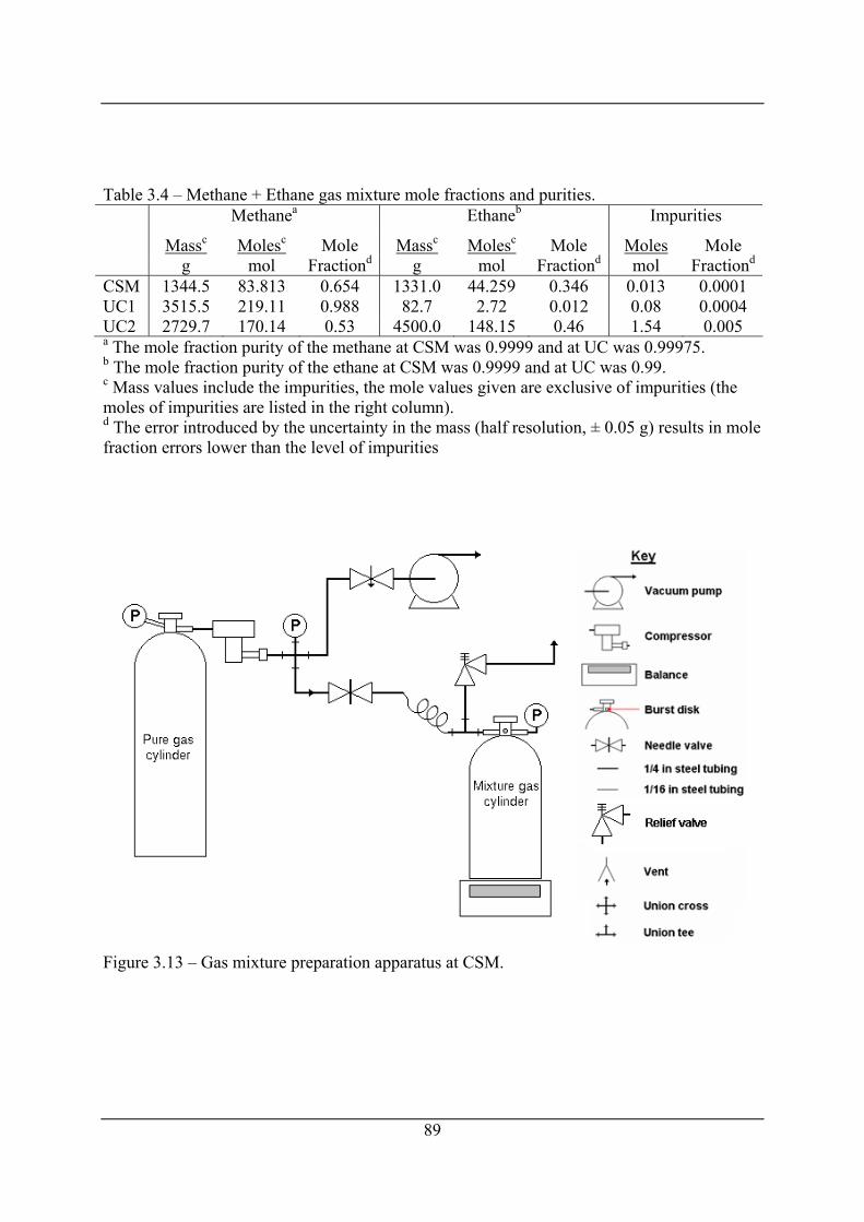
Table 3.4 – Methane + Ethane gas mixture mole fractions and purities. Methanea Ethaneb Impurities
Massc Molesc Mole Massc Molesc Mole Moles Mole g mol Fractiond g mol Fractiond mol Fractiond
CSM 1344.5 83.813 0.654 1331.0 44.259 0.346 0.013 0.0001 UC1 3515.5 219.11 0.988 82.7 2.72 0.012 0.08 0.0004 UC2 2729.7 170.14 0.53 4500.0 148.15 0.46 1.54 0.005 a The mole fraction purity of the methane at CSM was 0.9999 and at UC was 0.99975. b The mole fraction purity of the ethane at CSM was 0.9999 and at UC was 0.99. c Mass values include the impurities, the mole values given are exclusive of impurities (the moles of impurities are listed in the right column). d The error introduced by the uncertainty in the mass (half resolution, ± 0.05 g) results in mole fraction errors lower than the level of impurities
Figure 3.13 – Gas mixture preparation apparatus at CSM.
89
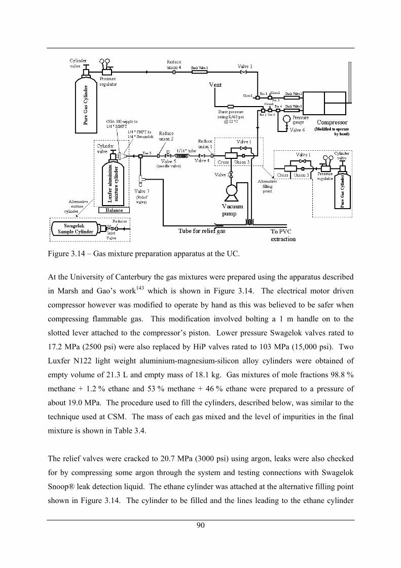
Figure 3.14 – Gas mixture preparation apparatus at the UC.
At the University of Canterbury the gas mixtures were prepared using the apparatus described
in Marsh and Gao’s work143 which is shown in Figure 3.14. The electrical motor driven
compressor however was modified to operate by hand as this was believed to be safer when
compressing flammable gas. This modification involved bolting a 1 m handle on to the
slotted lever attached to the compressor’s piston. Lower pressure Swagelok valves rated to
17.2 MPa (2500 psi) were also replaced by HiP valves rated to 103 MPa (15,000 psi). Two
Luxfer N122 light weight aluminium-magnesium-silicon alloy cylinders were obtained of
empty volume of 21.3 L and empty mass of 18.1 kg. Gas mixtures of mole fractions 98.8 %
methane + 1.2 % ethane and 53 % methane + 46 % ethane were prepared to a pressure of
about 19.0 MPa. The procedure used to fill the cylinders, described below, was similar to the
technique used at CSM. The mass of each gas mixed and the level of impurities in the final
mixture is shown in Table 3.4.
The relief valves were cracked to 20.7 MPa (3000 psi) using argon, leaks were also checked
for by compressing some argon through the system and testing connections with Swagelok
Snoop® leak detection liquid. The ethane cylinder was attached at the alternative filling point
shown in Figure 3.14. The cylinder to be filled and the lines leading to the ethane cylinder
90
91
were evacuated using the vacuum pump for at least two hours. Ethane was then purged into
the filling cylinder to a pressure of about 0.2 MPa and vacuuming was repeated. Once
vacuuming was complete the balance was tared. The extraction fan was then switched on and
the ethane cylinder valve was opened to allow gas to flow into the filling cylinder. The
ethane cylinder was insulated with fibre glass wool and heated with a heating cord to
encourage vaporization. Once the mass of ethane had reached the required value, as indicated
by the force balance, the cylinder valve on the filling cylinder was closed, the heater cord
switched off and the ethane cylinder valve was closed. The system lines were then
depressurised by slowly opening valve 1 to the extraction system. The ethane cylinder was
then disconnected and the methane cylinder attached at the alternative filling point. The lines
were then vacuumed for about 30 min. Methane was then introduced to the filling cylinder as
described for the ethane (but without heating) until the pressure of the methane dropped to
close to that of the filling cylinder. At this point the methane cylinder was detached and
reconnected at the pre-compressor filling point (top left Figure 3.14). An undesirable ethane
liquid layer will form in the cylinder at room temperature (20 °C) if the final filling density is
greater than 86.4 kg·m-3 (see Appendix E for a density-temperature diagram for ethane). This
was only a concern when preparing the 53 % methane + 46 % ethane mixture. If there is not
sufficient mixing the liquid ethane will remain in the liquid phase at a pressure near its vapour
pressure (since there is no methane in the liquid). When methane is added at a higher
pressure it will mix with the ethane vapour but the volume available for the vapour to fill is
reduced by the presence of the liquid ethane, this will result in a higher pressure of the
methane + ethane vapour phase than in the final properly mixed single phase mixture. Over-
pressurization can occur if this is not considered. For this reason mixing was initiated by
disconnecting the partly filled cylinder and inverting it about fifty times. The partly filled
cylinder was left to stand for an hour before it was reconnected to the system. The filling was
completed by compressing the methane. Firstly the methane cylinder valve was opened, and
gas was purged through the lines leading to the compressor. The compressor was then
operated for about ten strokes. This methane + air mixture in the lines was slowly vented into
the extraction duct by opening valve 1. The lines were purged thrice more to ensure that the
methane was sufficiently pure. The valve into the filling cylinder was then opened and
methane was compressed into the cylinder until the mass on the balance reached the final
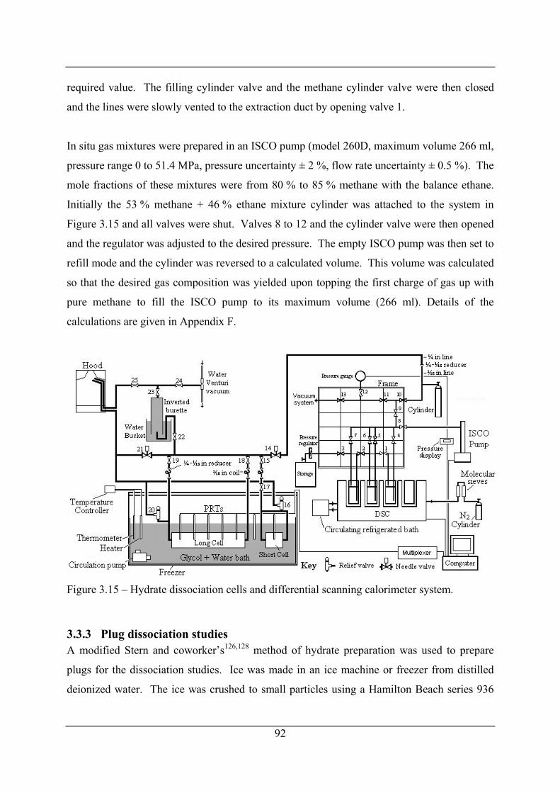
required value. The filling cylinder valve and the methane cylinder valve were then closed
and the lines were slowly vented to the extraction duct by opening valve 1.
In situ gas mixtures were prepared in an ISCO pump (model 260D, maximum volume 266 ml,
pressure range 0 to 51.4 MPa, pressure uncertainty ± 2 %, flow rate uncertainty ± 0.5 %). The
mole fractions of these mixtures were from 80 % to 85 % methane with the balance ethane.
Initially the 53 % methane + 46 % ethane mixture cylinder was attached to the system in
Figure 3.15 and all valves were shut. Valves 8 to 12 and the cylinder valve were then opened
and the regulator was adjusted to the desired pressure. The empty ISCO pump was then set to
refill mode and the cylinder was reversed to a calculated volume. This volume was calculated
so that the desired gas composition was yielded upon topping the first charge of gas up with
pure methane to fill the ISCO pump to its maximum volume (266 ml). Details of the
calculations are given in Appendix F.
Figure 3.15 – Hydrate dissociation cells and differential scanning calorimeter system.
3.3.3 Plug dissociation studies A modified Stern and coworker’s126,128 method of hydrate preparation was used to prepare
plugs for the dissociation studies. Ice was made in an ice machine or freezer from distilled
deionized water. The ice was crushed to small particles using a Hamilton Beach series 936
92
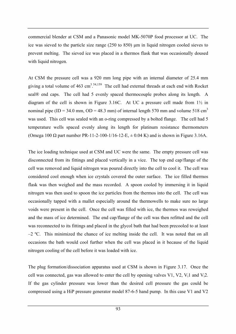
93
commercial blender at CSM and a Panasonic model MK-5070P food processor at UC. The
ice was sieved to the particle size range (250 to 850) μm in liquid nitrogen cooled sieves to
prevent melting. The sieved ice was placed in a thermos flask that was occasionally doused
with liquid nitrogen.
At CSM the pressure cell was a 920 mm long pipe with an internal diameter of 25.4 mm
giving a total volume of 463 cm3.54,159 The cell had external threads at each end with Rocket
seal® end caps. The cell had 5 evenly spaced thermocouple probes along its length. A
diagram of the cell is shown in Figure 3.16C. At UC a pressure cell made from 1½ in
nominal pipe (ID = 34.0 mm, OD = 48.3 mm) of internal length 570 mm and volume 518 cm3
was used. This cell was sealed with an o-ring compressed by a bolted flange. The cell had 5
temperature wells spaced evenly along its length for platinum resistance thermometers
(Omega 100 Ω part number PR-11-2-100-1/16-12-E, ± 0.04 K) and is shown in Figure 3.16A.
The ice loading technique used at CSM and UC were the same. The empty pressure cell was
disconnected from its fittings and placed vertically in a vice. The top end cap/flange of the
cell was removed and liquid nitrogen was poured directly into the cell to cool it. The cell was
considered cool enough when ice crystals covered the outer surface. The ice filled thermos
flask was then weighed and the mass recorded. A spoon cooled by immersing it in liquid
nitrogen was then used to spoon the ice particles from the thermos into the cell. The cell was
occasionally tapped with a mallet especially around the thermowells to make sure no large
voids were present in the cell. Once the cell was filled with ice, the thermos was reweighed
and the mass of ice determined. The end cap/flange of the cell was then refitted and the cell
was reconnected to its fittings and placed in the glycol bath that had been precooled to at least
–2 ºC. This minimized the chance of ice melting inside the cell. It was noted that on all
occasions the bath would cool further when the cell was placed in it because of the liquid
nitrogen cooling of the cell before it was loaded with ice.
The plug formation/dissociation apparatus used at CSM is shown in Figure 3.17. Once the
cell was connected, gas was allowed to enter the cell by opening valves V1, V2, Vi1 and Vi2.
If the gas cylinder pressure was lower than the desired cell pressure the gas could be
compressed using a HiP pressure generator model 87-6-5 hand pump. In this case V1 and V2
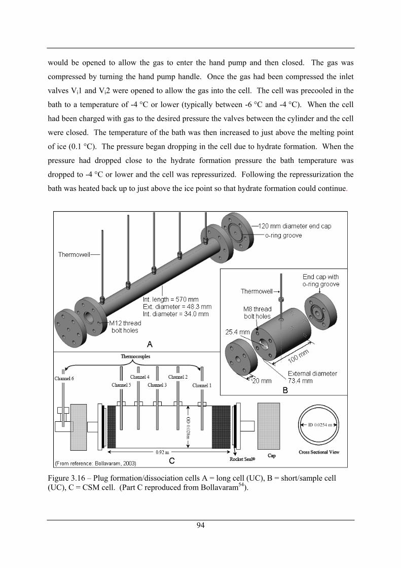
would be opened to allow the gas to enter the hand pump and then closed. The gas was
compressed by turning the hand pump handle. Once the gas had been compressed the inlet
valves Vi1 and Vi2 were opened to allow the gas into the cell. The cell was precooled in the
bath to a temperature of -4 °C or lower (typically between -6 °C and -4 °C). When the cell
had been charged with gas to the desired pressure the valves between the cylinder and the cell
were closed. The temperature of the bath was then increased to just above the melting point
of ice (0.1 °C). The pressure began dropping in the cell due to hydrate formation. When the
pressure had dropped close to the hydrate formation pressure the bath temperature was
dropped to -4 °C or lower and the cell was repressurized. Following the repressurization the
bath was heated back up to just above the ice point so that hydrate formation could continue.
Figure 3.16 – Plug formation/dissociation cells A = long cell (UC), B = short/sample cell (UC), C = CSM cell. (Part C reproduced from Bollavaram54).
94
Figure 3.17 – Plug dissociation apparatus at CSM.
The UC plug formation/dissociation apparatus is shown on the left of Figure 3.15. The
method of hydrate formation was initially (first two runs) by the pressure drop method as was
used at CSM, later formations however were carried out at constant pressure utilizing the
ISCO pump’s constant pressure mode. Pressure was more accurately read on the
Paroscientific pressure gauge (model 9000-6K-101, maximum pressure 41 MPa (6000 psi),
pressure uncertainty ± 0.01 %). The ISCO pump was filled by opening the cylinder regulator
and valves 8, 9 and 10 (valve numbers refer to valves in Figure 3.15) and running the pump in
the refill mode. The pressure was adjusted to approximately the calculated pressure for
hydrate formation. The valves to the cells in the glycol + water bath (valves 15, 17, 18 and
19) were then opened and the needle valve (valve 14) was slowly opened to allow gas to flow
to the cells. The ethylene glycol + water bath was cooled to -4 °C or lower before
pressurization began. The gas flow into the cells was slow to allow the gas to be cooled by
the bath. When the cell pressure had equalized with the desired pressure, the cylinder
regulator was closed and the ISCO pump was set to pump gas to maintain the desired
pressure. The bath temperature was then raised to 0.1 °C to allow hydrate formation to begin.
If the ISCO pump ran out of gas, valve 14 was closed and the bath chilled to below the ice
point (-4 °C or lower). The regulator was then opened to refill the pump. The cylinder
regulator was then closed, valve 14 reopened, and the ISCO pump was again set to pump to
maintain constant pressure. The bath temperature was then raised to just above the ice point
again.
95
96
At UC a short cell was placed in parallel to the long cell. The short cell was constructed with
an internal diameter of 25.4 mm, an external diameter of 144.0 mm and a length of 100 mm
with a total volume of 51 cm3 and is shown in Figure 3.16B (note: both the long cell and the
short cell were hydraulically pressure tested before they were used for experiments, see
Appendix G). Due to the short length of the cell, a thick wall along the entire length of the
cell was used rather than flanges with blind M8 threads of 35 mm and bolts sealed the end
plates. The purpose of the small cell was not for dissociation studies but to provide samples
that could be used for structural analysis and calorimetry, that should have the same structure
as the hydrates that were prepared in the long cell under the same formation conditions and
then dissociated.
Plug dissociations at both CSM and UC were carried out by the same method. The bath
temperature was raised to 4 °C and the system was then rapidly depressurized from both ends
of the cell. Gas flow from the hydrate cells was then directed to an inverted graduated burette
filled with water. The rate at which the water was displaced by the gas was measured with
stopwatches to give the hydrate dissociation rate. This rate was integrated over time and
multiplied by the molar density of the gas to give the moles of gas released as a function of
time.
3.3.4 Structural identification Structural analysis of the hydrates was carried out by Raman spectroscopy at CSM and
powder X-ray diffraction at UC.
Raman spectroscopy is a technique that measures the vibrational spectra of molecules (see
Chapter 2 of this work). Constraining a molecule in a hydrate cage will slightly alter the
vibrational spectra of a molecule. The Raman spectrometer at CSM was a Renishaw fibre
optic probe with an Argon laser as the excitation source. More detail of the apparatus may be
found in the Jager references.37,125 C-H and C-C vibrational frequencies for ethane in the
large cages of structures sI and sII are matched against literature values.36,71,94
To obtain samples for the Raman measurements at CSM the pressure cell was cooled in a bath
of liquid nitrogen. One end cap was removed and a sample of hydrate was scrapped out with
97
a cooled spoon. The disadvantage of this technique was that the remainder of the hydrate
could not be used for a plug dissociation measurement.
Structural analysis of samples at UC was by powder X-ray diffraction. As the crystal
structure of sI and sII hydrates are different they will produce a unique powder X-ray
diffraction pattern. Samples for powder X-ray diffraction were obtained from the short cell
by disconnecting it from the system before valves 16 and 17 (see Figure 3.15) and immersing
it in liquid nitrogen to cool the hydrate below its dissociation temperature at atmospheric
pressure. The cell was then opened to the atmosphere with valve 17 and the end flange was
removed. Samples were then scrapped out with a cooled spoon into a thermos of liquid
nitrogen. One end of a glass capillary (internal diameter = 0.3 mm) held with tweezers was
inserted repeatedly into the sample until it was covered with hydrate powder. The capillary
was then mounted, with the help of some petroleum jelly, onto the goniometer head of the X-
ray diffractometer in place of a mounting pin. The goniometer head was in a stream of
nitrogen gas at -180 °C to prevent hydrate dissociation. The X-ray tube (Mo Kα) was then
switched on and a pattern was recorded with the Bruker Smart CCD area-detector
diffractometer. Usually this instrument is used to collect single crystal X-ray diffraction data
but it can, as in this case, also be used to collect powder diffraction data if the 360 ° phi drive
and scan function is used.
3.3.5 Calorimetry The calorimeter used in this work is shown on the right hand side of Figure 3.15. The
calorimeter is a Calorimetry Sciences Corporation 4100 multi-cell differential scanning
calorimeter (MC-DSC) with a high pressure kit for measurements up to 14.0 MPa. Details of
the calorimeter’s uncertainties, setabilities and stabilities are shown in Table 3.5. The
calorimeter has four cells (one reference cell and 3 measurement cells) of about 1 ml in
volume. The MC-DSC’s high pressure cells each have two 1/16 in stainless steel tubing
connections. The inlet tube extends to near the bottom of the cell whereas the outlet tube runs
from the top of the cell.
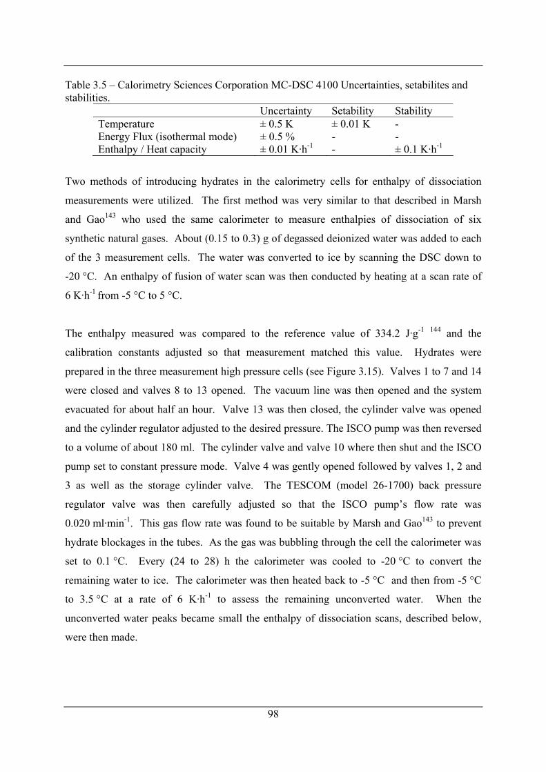
98
Table 3.5 – Calorimetry Sciences Corporation MC-DSC 4100 Uncertainties, setabilites and stabilities.
Uncertainty Setability Stability Temperature ± 0.5 K ± 0.01 K - Energy Flux (isothermal mode) ± 0.5 % - - Enthalpy / Heat capacity ± 0.01 K·h-1 - ± 0.1 K·h-1
Two methods of introducing hydrates in the calorimetry cells for enthalpy of dissociation
measurements were utilized. The first method was very similar to that described in Marsh
and Gao143 who used the same calorimeter to measure enthalpies of dissociation of six
synthetic natural gases. About (0.15 to 0.3) g of degassed deionized water was added to each
of the 3 measurement cells. The water was converted to ice by scanning the DSC down to
-20 °C. An enthalpy of fusion of water scan was then conducted by heating at a scan rate of
6 K·h-1 from -5 °C to 5 °C.
The enthalpy measured was compared to the reference value of 334.2 J·g-1 144 and the
calibration constants adjusted so that measurement matched this value. Hydrates were
prepared in the three measurement high pressure cells (see Figure 3.15). Valves 1 to 7 and 14
were closed and valves 8 to 13 opened. The vacuum line was then opened and the system
evacuated for about half an hour. Valve 13 was then closed, the cylinder valve was opened
and the cylinder regulator adjusted to the desired pressure. The ISCO pump was then reversed
to a volume of about 180 ml. The cylinder valve and valve 10 where then shut and the ISCO
pump set to constant pressure mode. Valve 4 was gently opened followed by valves 1, 2 and
3 as well as the storage cylinder valve. The TESCOM (model 26-1700) back pressure
regulator valve was then carefully adjusted so that the ISCO pump’s flow rate was
0.020 ml·min-1. This gas flow rate was found to be suitable by Marsh and Gao143 to prevent
hydrate blockages in the tubes. As the gas was bubbling through the cell the calorimeter was
set to 0.1 °C. Every (24 to 28) h the calorimeter was cooled to -20 °C to convert the
remaining water to ice. The calorimeter was then heated back to -5 °C and then from -5 °C
to 3.5 °C at a rate of 6 K·h-1 to assess the remaining unconverted water. When the
unconverted water peaks became small the enthalpy of dissociation scans, described below,
were then made.
99
Valve 3 was closed and valves 5 to 7 opened. The calorimeter was then cooled to -20 °C for a
period of 30 min to convert remaining water to ice. The calorimeter was then heated at it
maximum scan rate (120 K·h-1 or 2 K·min-1) to -5 °C, it was then heated at the lower scan rate
of 6 K·h-1 (0.1 K·min-1) from -5 °C to 3.5 °C to obtain an enthalpy of fusion peak for the
unconverted water. The ISCO pump was then stopped as Marsh and Gao143 reported that gas
flow could disturb the calorimetric response. The calorimeter was then set to scan from 5 °C
below to 8 °C above the predicted hydrate dissociation temperature (from CSMGem) at
6 K·h-1 (0.1 K·min-1). Pressure change during hydrate dissociation was not more than 0.022
MPa so the hydrate dissociation could be considered isobaric.
The amount of water in each cell was then measured by an enthalpy of fusion of water scan.
The system had to be depressurized first to prevent hydrates reforming when the temperature
was lowered below the dissociation temperature. Starting with valves 1 to 8, 10 and 13 closed
the system was depressurized by opening valve 10, 14 and 21 and then releasing the pressure
to below the hydrate formation pressure at -20 °C, this pressure was typically about 1.0 MPa.
The hydrate cells were then depressurized by slowly opening valves 7, then 6, 5, 1, 2 and
finally 4. The calorimeter was cooled down to -20 °C to convert the water in the cells to ice
then an enthalpy of fusion of ice scan was conducted by heating the calorimeter from -5 °C to
5 °C at a rate of 6 K·h-1. This scan enabled the mass of water in each calorimeter cell to be
calculated by use of the standard enthalpy of 334.2 J·g-1.144 This mass along with the
predissociation mass of unconverted ice allowed calculation of the mass of water associated
with the hydrate. This along with a hydrate number predicted using CSMGem allowed the
calculation of a dissociation enthalpy. This method of in-calorimeter-cell hydrate formation
and dissociation were used to measure the enthalpy of dissociation of a sII hydrate prepared
from a gas of mole fractions 98.8 % methane + 1.2 % ethane.
The second method of introducing hydrates into the calorimeter involved cryogenic transfer
from the sample cell. The small cell was immersed in liquid nitrogen in a polystyrene
container. The cell and contents were allowed to cool to the liquid nitrogen boiling point of
-196 °C. At this temperature the hydrate is stable at atmospheric pressure and thus can be
stored in a Dewar flask of liquid nitrogen indefinitely.
100
The transfer technique to the calorimeter involved immersing the bottom of the high pressure
calorimetry cells in liquid nitrogen until they had cooled. The top of the cell was not directly
contacted with the liquid nitrogen so not to overcool the area around the o-ring seal. A lump
of hydrate of suitable size (of approximate radius 5 mm or less) was removed from the storage
Dewar flask with cooled tweezers and immediately placed into the calorimeter cell. The
calorimeter cell was then sealed and pressurized to a pressure high enough to stabilize the
hydrate at about room temperature. The cell was allowed to heat up to room temperature and
any atmospheric water that condensed on the outside of the cell was carefully wiped off with
a lint free cloth. When the cell reached approximately room temperature it was placed inside
the calorimeter. This technique was repeated until all three working cells of the calorimeter
contained a sample. The pressure of the calorimeter cell was then slowly adjusted to the
desired pressure using the ISCO pump. The hydrate was allowed to equilibrate in the cells for
at least 24 h before any measurements were taken.
The hydrate dissociation enthalpy was measured by first conducting an enthalpy of fusion of
ice scan. The calorimeter was scanned down to -20 °C to convert any remaining water to ice.
The cells where then heated from -5 °C to +5 °C at a scan rate of 6 K·h-1. The ISCO pump
was then switched off as it had been found to disturb scan results.143 The enthalpy of
dissociation scan was then started from about 5 °C below the expected dissociation
temperature to about 8 °C above the predicted dissociation temperature at a scan rate of
6 K·h-1. The mass of hydrate was determined as for the other method of hydrate formation in
the calorimeter (by a pre-hydrate dissociation ice scan to find the mass of unconverted ice and
a post-hydrate dissociation ice scan to find the total amount of ice).
The cryogenic transfer method was used to load hydrate formed in the small cell of the (UC)
plug dissociation apparatus from an ISCO pump prepared mixture of mole fraction 80 %
methane + 20 % ethane. This plug was formed at a constant pressure of 4 MPa and was
structurally analysed as a sII plug by X-ray diffraction. The hydrate phase composition was
believed to be similar to that prepared by the flow method in the calorimeter from the gas
mixture of mole fraction 98.8 % methane + 1.2 % ethane due to “preferential enclathration”
of ethane in the hydrate phase in the high mole ratio of water to gas system of the plug
formation cells. Preferential enclathration is a phenomenon where the hydrate phase
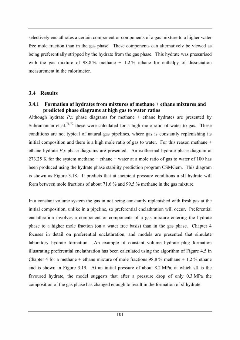
101
selectively enclathrates a certain component or components of a gas mixture to a higher water
free mole fraction than in the gas phase. These components can alternatively be viewed as
being preferentially stripped by the hydrate from the gas phase. This hydrate was pressurised
with the gas mixture of 98.8 % methane + 1.2 % ethane for enthalpy of dissociation
measurement in the calorimeter.
3.4 Results
3.4.1 Formation of hydrates from mixtures of methane + ethane mixtures and predicted phase diagrams at high gas to water ratios
Although hydrate P,x phase diagrams for methane + ethane hydrates are presented by
Subramanian et al.71,72 these were calculated for a high mole ratio of water to gas. These
conditions are not typical of natural gas pipelines, where gas is constantly replenishing its
initial composition and there is a high mole ratio of gas to water. For this reason methane +
ethane hydrate P,x phase diagrams are presented. An isothermal hydrate phase diagram at
273.25 K for the system methane + ethane + water at a mole ratio of gas to water of 100 has
been produced using the hydrate phase stability prediction program CSMGem. This diagram
is shown as Figure 3.18. It predicts that at incipient pressure conditions a sII hydrate will
form between mole fractions of about 71.6 % and 99.5 % methane in the gas mixture.
In a constant volume system the gas in not being constantly replenished with fresh gas at the
initial composition, unlike in a pipeline, so preferential enclathration will occur. Preferential
enclathration involves a component or components of a gas mixture entering the hydrate
phase to a higher mole fraction (on a water free basis) than in the gas phase. Chapter 4
focuses in detail on preferential enclathration, and models are presented that simulate
laboratory hydrate formation. An example of constant volume hydrate plug formation
illustrating preferential enclathration has been calculated using the algorithm of Figure 4.5 in
Chapter 4 for a methane + ethane mixture of mole fractions 98.8 % methane + 1.2 % ethane
and is shown in Figure 3.19. At an initial pressure of about 8.2 MPa, at which sII is the
favoured hydrate, the model suggests that after a pressure drop of only 0.3 MPa the
composition of the gas phase has changed enough to result in the formation of sI hydrate.
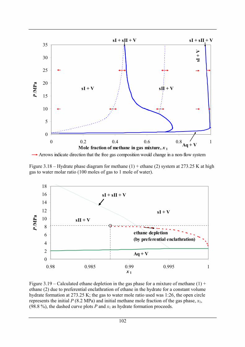
0
5
10
15
20
25
30
35
0 0.2 0.4 0.6 0.8 1Mole fraction of methane in gas mixture, x 1
P/M
Pa
Aq + V
sI + V sII + V
sI + sII + V
sI +
V
sI + sII + V
Arrows indicate direction that the free gas composition would change in a non-flow system
Figure 3.18 – Hydrate phase diagram for methane (1) + ethane (2) system at 273.25 K at high gas to water molar ratio (100 moles of gas to 1 mole of water).
024
68
1012
141618
0.98 0.985 0.99 0.995 1x 1
P/M
Pa
Aq + V
sI + VsII + V
sI + sII + V
ethane depletion(by preferential enclathration)
Figure 3.19 – Calculated ethane depletion in the gas phase for a mixture of methane (1) + ethane (2) due to preferential enclathration of ethane in the hydrate for a constant volume hydrate formation at 273.25 K; the gas to water mole ratio used was 1:26, the open circle represents the initial P (8.2 MPa) and initial methane mole fraction of the gas phase, x1, (98.8 %), the dashed curve plots P and x1 as hydrate formation proceeds.
102
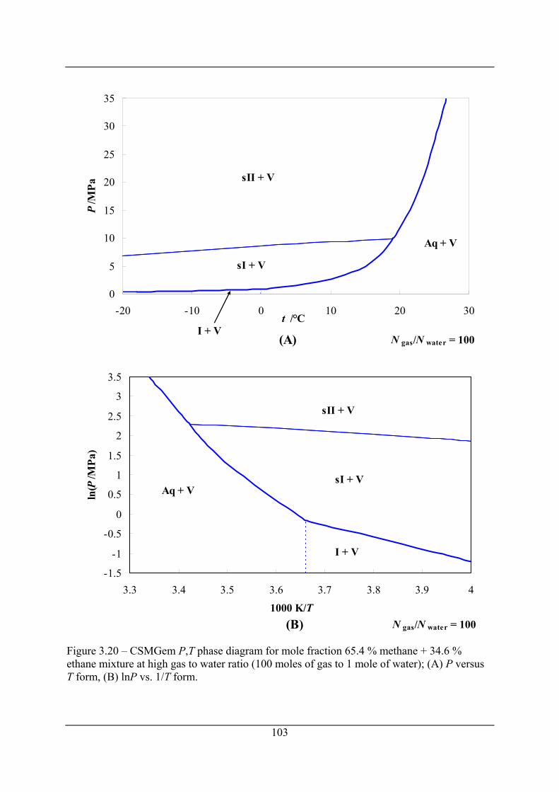
0
5
10
15
20
25
30
35
-20 -10 0 10 20 3t /°C
P/M
Pa
sI + V
sII + V
Aq + V
0
N gas/N water = 100I + V
(A)
-1.5
-1
-0.5
0
0.5
1
1.5
2
2.5
3
3.5
3.3 3.4 3.5 3.6 3.7 3.8 3.9 41000 K/T
ln(P
/MPa
)
sI + VAq + V
sII + V
I + V
N gas/N water = 100(B)
Figure 3.20 – CSMGem P,T phase diagram for mole fraction 65.4 % methane + 34.6 % ethane mixture at high gas to water ratio (100 moles of gas to 1 mole of water); (A) P versus T form, (B) lnP vs. 1/T form.
103
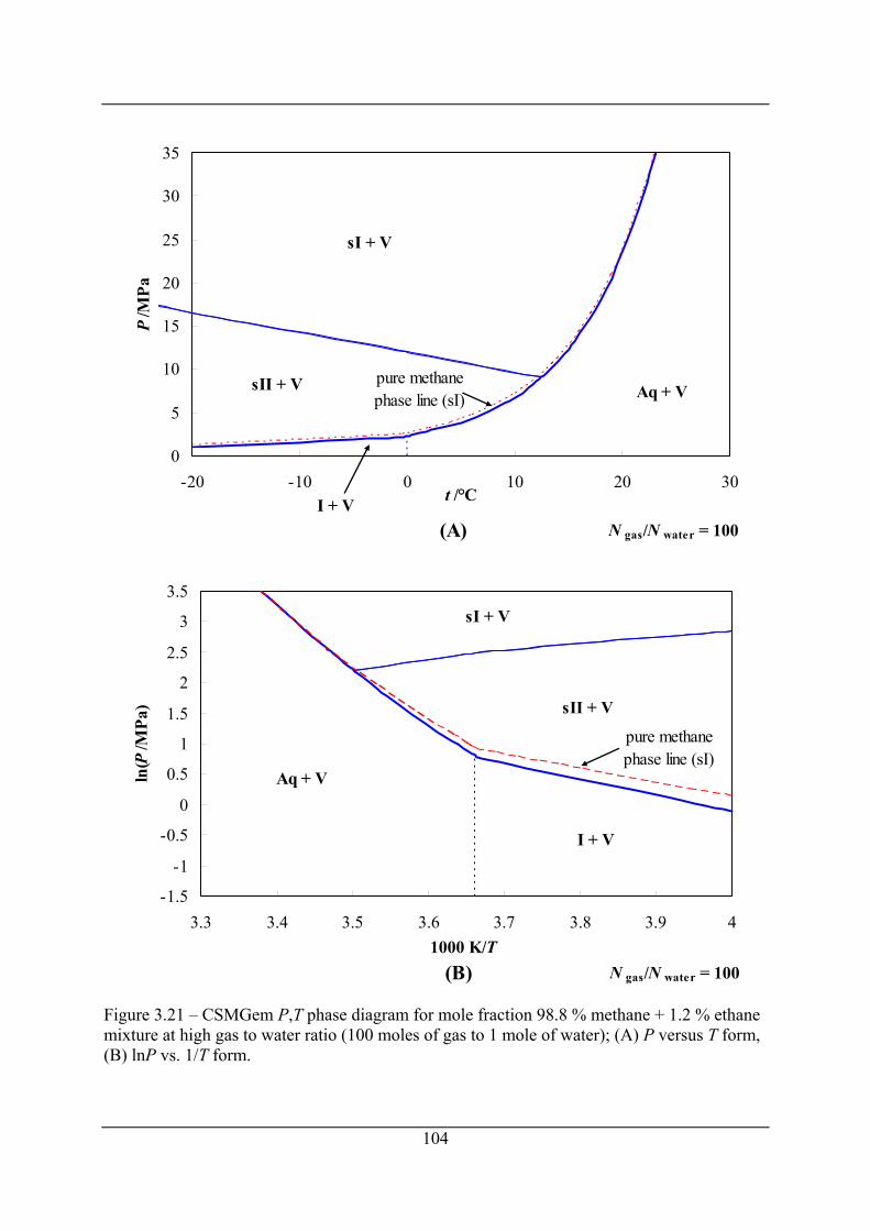
-1.5
-1
-0.5
0
0.5
1
1.5
2
2.5
3
3.5
3.3 3.4 3.5 3.6 3.7 3.8 3.9 41000 K/T
ln(P
/MPa
)
sI + V
Aq + V
sII + V
I + V
pure methanephase line (sI)
N gas/N water = 100(B)
0
5
10
15
20
25
30
35
-20 -10 0 10 20 3t /°C
P/M
Pa
sI + V
sII + V Aq + Vpure methanephase line (sI)
0
N gas/N water = 100I + V
(A)
Figure 3.21 – CSMGem P,T phase diagram for mole fraction 98.8 % methane + 1.2 % ethane mixture at high gas to water ratio (100 moles of gas to 1 mole of water); (A) P versus T form, (B) lnP vs. 1/T form.
104
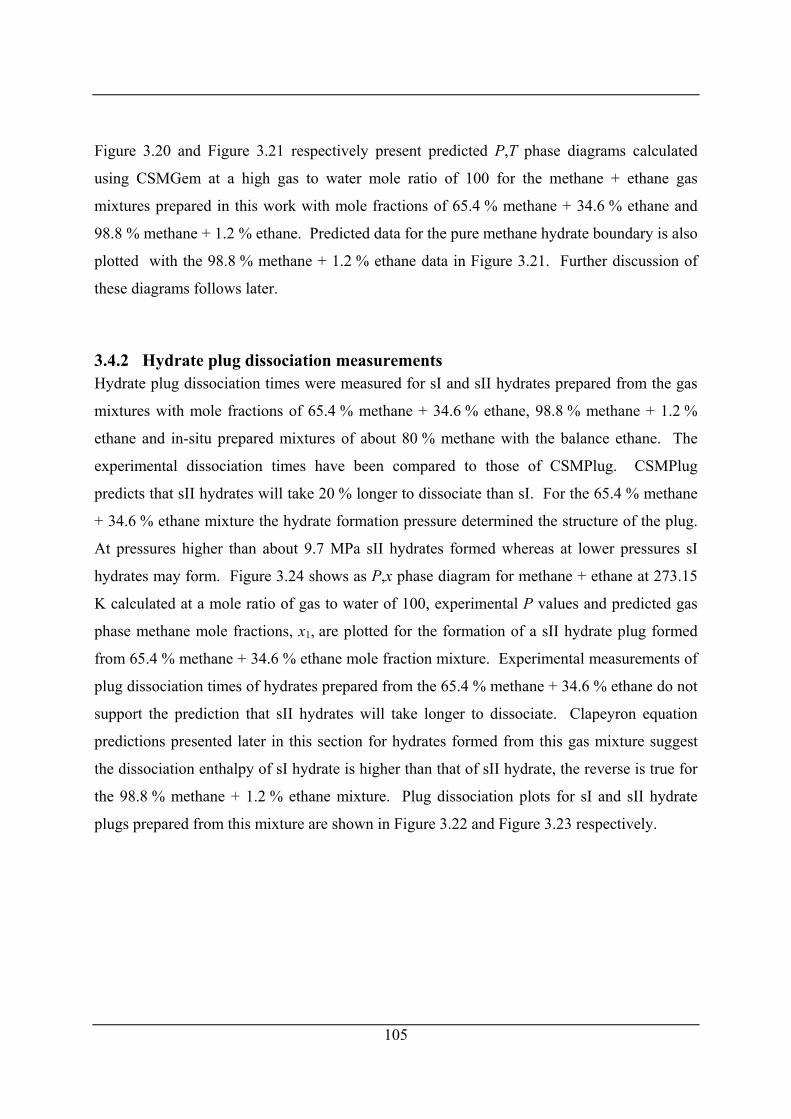
105
Figure 3.20 and Figure 3.21 respectively present predicted P,T phase diagrams calculated
using CSMGem at a high gas to water mole ratio of 100 for the methane + ethane gas
mixtures prepared in this work with mole fractions of 65.4 % methane + 34.6 % ethane and
98.8 % methane + 1.2 % ethane. Predicted data for the pure methane hydrate boundary is also
plotted with the 98.8 % methane + 1.2 % ethane data in Figure 3.21. Further discussion of
these diagrams follows later.
3.4.2 Hydrate plug dissociation measurements Hydrate plug dissociation times were measured for sI and sII hydrates prepared from the gas
mixtures with mole fractions of 65.4 % methane + 34.6 % ethane, 98.8 % methane + 1.2 %
ethane and in-situ prepared mixtures of about 80 % methane with the balance ethane. The
experimental dissociation times have been compared to those of CSMPlug. CSMPlug
predicts that sII hydrates will take 20 % longer to dissociate than sI. For the 65.4 % methane
+ 34.6 % ethane mixture the hydrate formation pressure determined the structure of the plug.
At pressures higher than about 9.7 MPa sII hydrates formed whereas at lower pressures sI
hydrates may form. Figure 3.24 shows as P,x phase diagram for methane + ethane at 273.15
K calculated at a mole ratio of gas to water of 100, experimental P values and predicted gas
phase methane mole fractions, x1, are plotted for the formation of a sII hydrate plug formed
from 65.4 % methane + 34.6 % ethane mole fraction mixture. Experimental measurements of
plug dissociation times of hydrates prepared from the 65.4 % methane + 34.6 % ethane do not
support the prediction that sII hydrates will take longer to dissociate. Clapeyron equation
predictions presented later in this section for hydrates formed from this gas mixture suggest
the dissociation enthalpy of sI hydrate is higher than that of sII hydrate, the reverse is true for
the 98.8 % methane + 1.2 % ethane mixture. Plug dissociation plots for sI and sII hydrate
plugs prepared from this mixture are shown in Figure 3.22 and Figure 3.23 respectively.
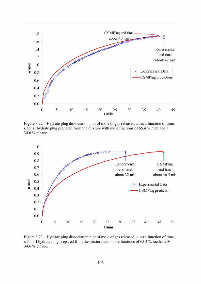
0.0
0.2
0.4
0.6
0.8
1.0
1.2
1.4
1.6
1.8
0 5 10 15 20 25 30 35 40 45t /min
n/m
ol
Experimental DataCSMPlug prediction
Experimentalend time
about 42 min
CSMPlug end time about 40 min
Figure 3.22 – Hydrate plug dissociation plot of mole of gas released, n, as a function of time, t, for sI hydrate plug prepared from the mixture with mole fractions of 65.4 % methane + 34.6 % ethane.
0.0
0.1
0.2
0.3
0.4
0.5
0.6
0.7
0.8
0.9
1.0
0 5 10 15 20 25 30 35 40 45 50t /min
n/m
ol
Experimental DataCSMPlug prediction
Experimentalend time
about 32 min
CSMPlugend time
about 46.5 min
Figure 3.23 – Hydrate plug dissociation plot of mole of gas released, n, as a function of time, t, for sII hydrate plug prepared from the mixture with mole fractions of 65.4 % methane + 34.6 % ethane.
106
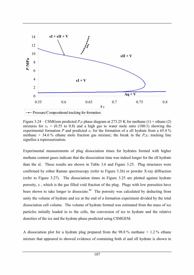
0
2
4
6
8
10
12
14
0.55 0.6 0.65 0.7 0.75 0.8x 1
P/M
Pa
Pressure/Compositional tracking for formation
Aq + V
sI + V
sII + V
sI + sII + V
Figure 3.24 – CSMGem predicted P,x phase diagram at 273.25 K for methane (1) + ethane (2) mixtures for x1 = (0.55 to 0.8) and a high gas to water mole ratio (100:1) showing the experimental formation P and predicted x1 for the formation of a sII hydrate from a 65.4 % methane + 34.6 % ethane mole fraction gas mixture; the break in the P,x1 tracking line signifies a repressurization.
Experimental measurements of plug dissociation times for hydrates formed with higher
methane content gases indicate that the dissociation time was indeed longer for the sII hydrate
than the sI. These results are shown in Table 3.6 and Figure 3.25. Plug structures were
confirmed by either Raman spectroscopy (refer to Figure 3.26) or powder X-ray diffraction
(refer to Figure 3.27). The dissociation times in Figure 3.25 are plotted against hydrate
porosity, ε , which is the gas filled void fraction of the plug. Plugs with low porosities have
been shown to take longer to dissociate.49 The porosity was calculated by deducting from
unity the volume of hydrate and ice at the end of a formation experiment divided by the total
dissociation cell volume. The volume of hydrate formed was estimated from the mass of ice
particles initially loaded in to the cells, the conversion of ice to hydrate and the relative
densities of the ice and the hydrate phase predicted using CSMGEM.
A dissociation plot for a hydrate plug prepared from the 98.8 % methane + 1.2 % ethane
mixture that appeared to showed evidence of containing both sI and sII hydrate is shown in
107
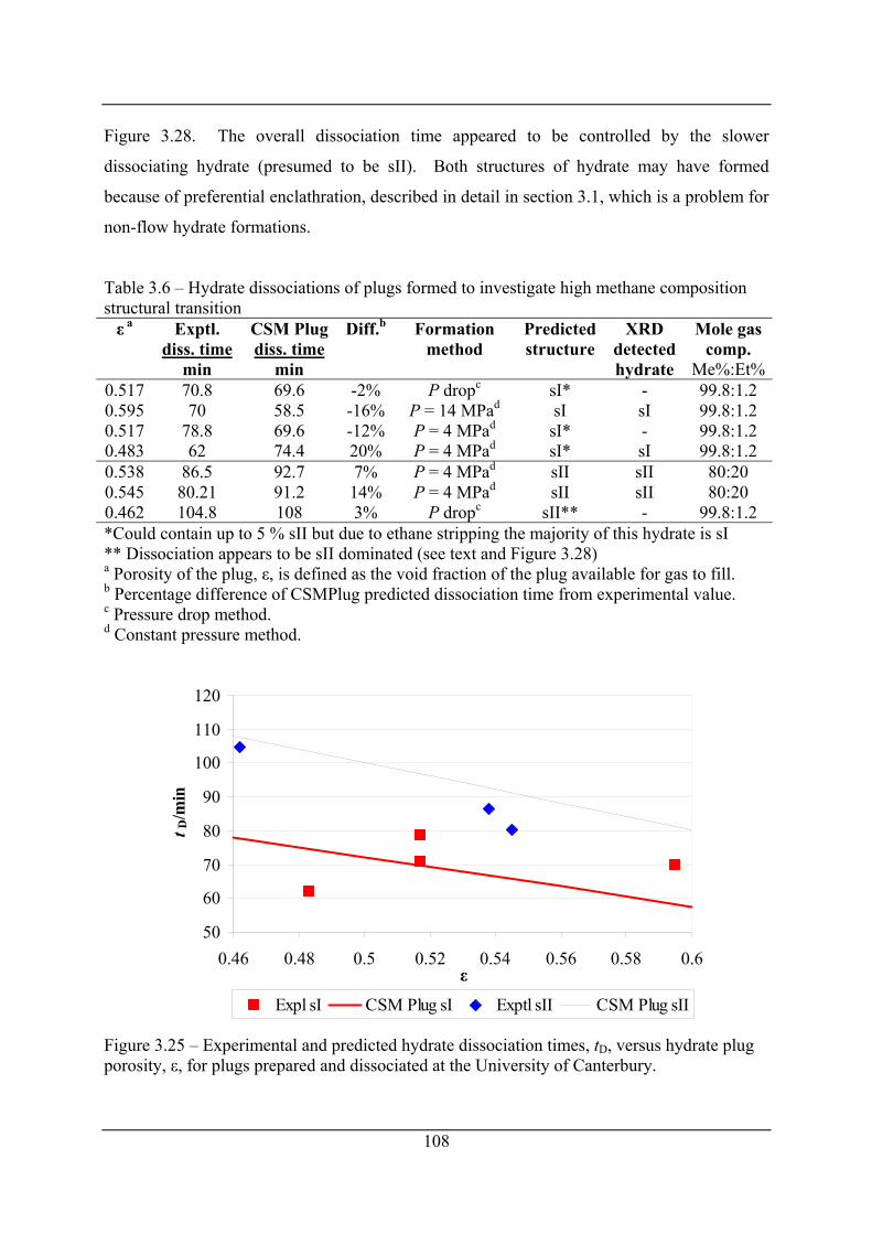
Figure 3.28. The overall dissociation time appeared to be controlled by the slower
dissociating hydrate (presumed to be sII). Both structures of hydrate may have formed
because of preferential enclathration, described in detail in section 3.1, which is a problem for
non-flow hydrate formations.
Table 3.6 – Hydrate dissociations of plugs formed to investigate high methane composition structural transition ε a Exptl. CSM Plug Diff.b Formation Predicted XRD Mole gas diss. time diss. time method structure detected comp. min min hydrate Me%:Et%
0.517 70.8 69.6 -2% P dropc sI* - 99.8:1.2 0.595 70 58.5 -16% P = 14 MPad sI sI 99.8:1.2 0.517 78.8 69.6 -12% P = 4 MPad sI* - 99.8:1.2 0.483 62 74.4 20% P = 4 MPad sI* sI 99.8:1.2 0.538 86.5 92.7 7% P = 4 MPad sII sII 80:20 0.545 80.21 91.2 14% P = 4 MPad sII sII 80:20 0.462 104.8 108 3% P dropc sII** - 99.8:1.2 *Could contain up to 5 % sII but due to ethane stripping the majority of this hydrate is sI ** Dissociation appears to be sII dominated (see text and Figure 3.28) a Porosity of the plug, ε, is defined as the void fraction of the plug available for gas to fill. b Percentage difference of CSMPlug predicted dissociation time from experimental value. c Pressure drop method. d Constant pressure method.
50
60
70
80
90
100
110
120
0.46 0.48 0.5 0.52 0.54 0.56 0.58 0.6ε
t D/m
in
Expl sI CSM Plug sI Exptl sII CSM Plug sII
Figure 3.25 – Experimental and predicted hydrate dissociation times, tD, versus hydrate plug porosity, ε, for plugs prepared and dissociated at the University of Canterbury.
108
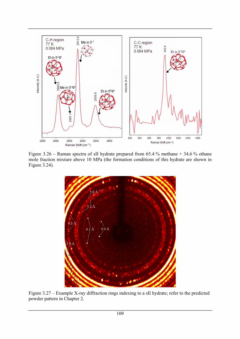
Figure 3.26 – Raman spectra of sII hydrate prepared from 65.4 % methane + 34.6 % ethane mole fraction mixture above 10 MPa (the formation conditions of this hydrate are shown in Figure 3.24).
Figure 3.27 – Example X-ray diffraction rings indexing to a sII hydrate; refer to the predicted powder pattern in Chapter 2.
109
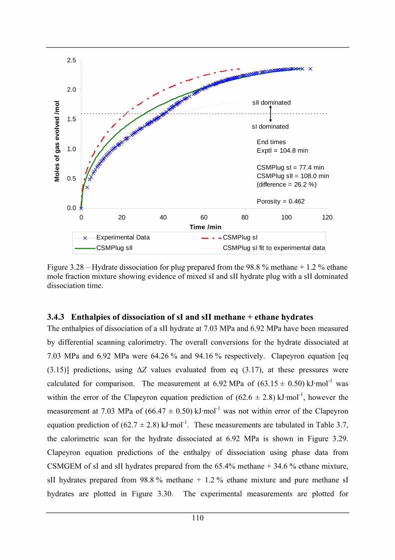
0.0
0.5
1.0
1.5
2.0
2.5
0 20 40 60 80 100Time /min
Mol
es o
f gas
evo
lved
/mol
120
Experimental Data CSMPlug sICSMPlug sII CSMPlug sI fit to experimental data
End timesExptl = 104.8 min
CSMPlug sI = 77.4 minCSMPlug sII = 108.0 min(difference = 26.2 %)
Porosity = 0.462
sI dominated
sII dominated
Figure 3.28 – Hydrate dissociation for plug prepared from the 98.8 % methane + 1.2 % ethane mole fraction mixture showing evidence of mixed sI and sII hydrate plug with a sII dominated dissociation time.
3.4.3 Enthalpies of dissociation of sI and sII methane + ethane hydrates The enthalpies of dissociation of a sII hydrate at 7.03 MPa and 6.92 MPa have been measured
by differential scanning calorimetry. The overall conversions for the hydrate dissociated at
7.03 MPa and 6.92 MPa were 64.26 % and 94.16 % respectively. Clapeyron equation [eq
(3.15)] predictions, using ΔZ values evaluated from eq (3.17), at these pressures were
calculated for comparison. The measurement at 6.92 MPa of (63.15 ± 0.50) kJ·mol-1 was
within the error of the Clapeyron equation prediction of (62.6 ± 2.8) kJ·mol-1, however the
measurement at 7.03 MPa of (66.47 ± 0.50) kJ·mol-1 was not within error of the Clapeyron
equation prediction of (62.7 ± 2.8) kJ·mol-1. These measurements are tabulated in Table 3.7,
the calorimetric scan for the hydrate dissociated at 6.92 MPa is shown in Figure 3.29.
Clapeyron equation predictions of the enthalpy of dissociation using phase data from
CSMGEM of sI and sII hydrates prepared from the 65.4% methane + 34.6 % ethane mixture,
sII hydrates prepared from 98.8 % methane + 1.2 % ethane mixture and pure methane sI
hydrates are plotted in Figure 3.30. The experimental measurements are plotted for
110
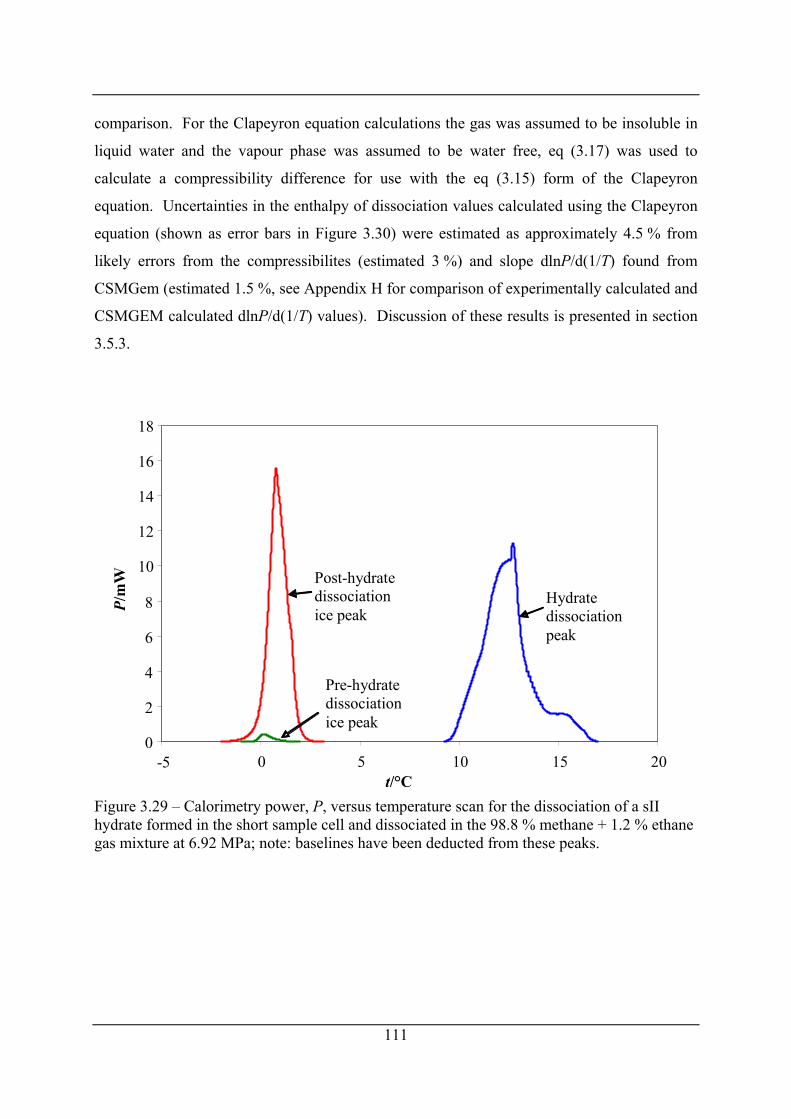
comparison. For the Clapeyron equation calculations the gas was assumed to be insoluble in
liquid water and the vapour phase was assumed to be water free, eq (3.17) was used to
calculate a compressibility difference for use with the eq (3.15) form of the Clapeyron
equation. Uncertainties in the enthalpy of dissociation values calculated using the Clapeyron
equation (shown as error bars in Figure 3.30) were estimated as approximately 4.5 % from
likely errors from the compressibilites (estimated 3 %) and slope dlnP/d(1/T) found from
CSMGem (estimated 1.5 %, see Appendix H for comparison of experimentally calculated and
CSMGEM calculated dlnP/d(1/T) values). Discussion of these results is presented in section
3.5.3.
0
2
4
6
8
10
12
14
16
18
-5 0 5 10 15 20t/°C
P/m
W
Post-hydratedissociation ice peak
Hydrate dissociation peak
Pre-hydrate dissociation ice peak
Figure 3.29 – Calorimetry power, P, versus temperature scan for the dissociation of a sII hydrate formed in the short sample cell and dissociated in the 98.8 % methane + 1.2 % ethane gas mixture at 6.92 MPa; note: baselines have been deducted from these peaks.
111
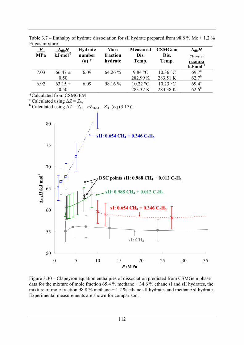
Table 3.7 – Enthalpy of hydrate dissociation for sII hydrate prepared from 98.8 % Me + 1.2 % Et gas mixture.
_P_ MPa
_ΔdisH_ kJ·mol-1
Hydrate number
(n) *
Mass fraction hydrate
MeasuredDis.
Temp.
CSMGem Dis.
Temp.
ΔdisH
Clapeyron
CSMGEM kJ·mol-1
7.03 66.47 ± 0.50
6.09 64.26 % 9.84 °C 282.99 K
10.36 °C 283.51 K
69.7a 62.7b
6.92 63.15 ± 0.50
6.09 98.16 % 10.22 °C 283.37 K
10.23 °C 283.38 K
69.4a 62.6b
*Calculated from CSMGEM
a Calculated using ΔZ = ZG, b Calculated using ΔZ = ZG – nZH2O – ZH (eq (3.17)).
50
55
60
65
70
75
80
0 5 10 15 20 25 30 35P /MPa
Δ dis
H/k
J·m
ol-1
sII: 0.654 CH4 + 0.346 C2H6
sI: CH4
DSC points sII: 0.988 CH4 + 0.012 C2H6
sII: 0.988 CH4 + 0.012 C2H6
sI: 0.654 CH4 + 0.346 C2H6
Figure 3.30 – Clapeyron equation enthalpies of dissociation predicted from CSMGem phase data for the mixture of mole fraction 65.4 % methane + 34.6 % ethane sI and sII hydrates, the mixture of mole fraction 98.8 % methane + 1.2 % ethane sII hydrates and methane sI hydrate. Experimental measurements are shown for comparison.
112
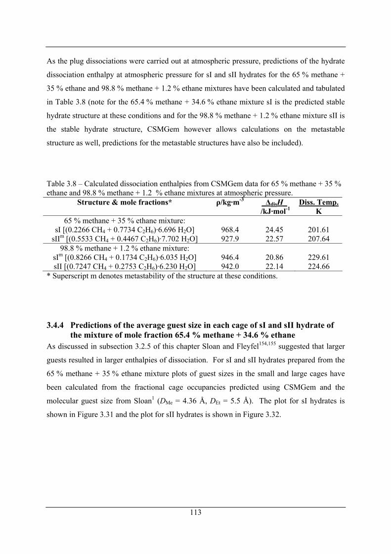
113
As the plug dissociations were carried out at atmospheric pressure, predictions of the hydrate
dissociation enthalpy at atmospheric pressure for sI and sII hydrates for the 65 % methane +
35 % ethane and 98.8 % methane + 1.2 % ethane mixtures have been calculated and tabulated
in Table 3.8 (note for the 65.4 % methane + 34.6 % ethane mixture sI is the predicted stable
hydrate structure at these conditions and for the 98.8 % methane + 1.2 % ethane mixture sII is
the stable hydrate structure, CSMGem however allows calculations on the metastable
structure as well, predictions for the metastable structures have also be included).
Table 3.8 – Calculated dissociation enthalpies from CSMGem data for 65 % methane + 35 % ethane and 98.8 % methane + 1.2 % ethane mixtures at atmospheric pressure.
Structure & mole fractions* ρ/kg·m-3 _ΔdisH_ /kJ·mol-1
Diss. Temp. K
65 % methane + 35 % ethane mixture: sI [(0.2266 CH4 + 0.7734 C2H6)·6.696 H2O] 968.4 24.45 201.61
sIIm [(0.5533 CH4 + 0.4467 C2H6)·7.702 H2O] 927.9 22.57 207.64 98.8 % methane + 1.2 % ethane mixture:
sIm [(0.8266 CH4 + 0.1734 C2H6)·6.035 H2O] 946.4 20.86 229.61 sII [(0.7247 CH4 + 0.2753 C2H6)·6.230 H2O] 942.0 22.14 224.66
* Superscript m denotes metastability of the structure at these conditions.
3.4.4 Predictions of the average guest size in each cage of sI and sII hydrate of the mixture of mole fraction 65.4 % methane + 34.6 % ethane
As discussed in subsection 3.2.5 of this chapter Sloan and Fleyfel154,155 suggested that larger
guests resulted in larger enthalpies of dissociation. For sI and sII hydrates prepared from the
65 % methane + 35 % ethane mixture plots of guest sizes in the small and large cages have
been calculated from the fractional cage occupancies predicted using CSMGem and the
molecular guest size from Sloan1 (DMe = 4.36 Å, DEt = 5.5 Å). The plot for sI hydrates is
shown in Figure 3.31 and the plot for sII hydrates is shown in Figure 3.32.
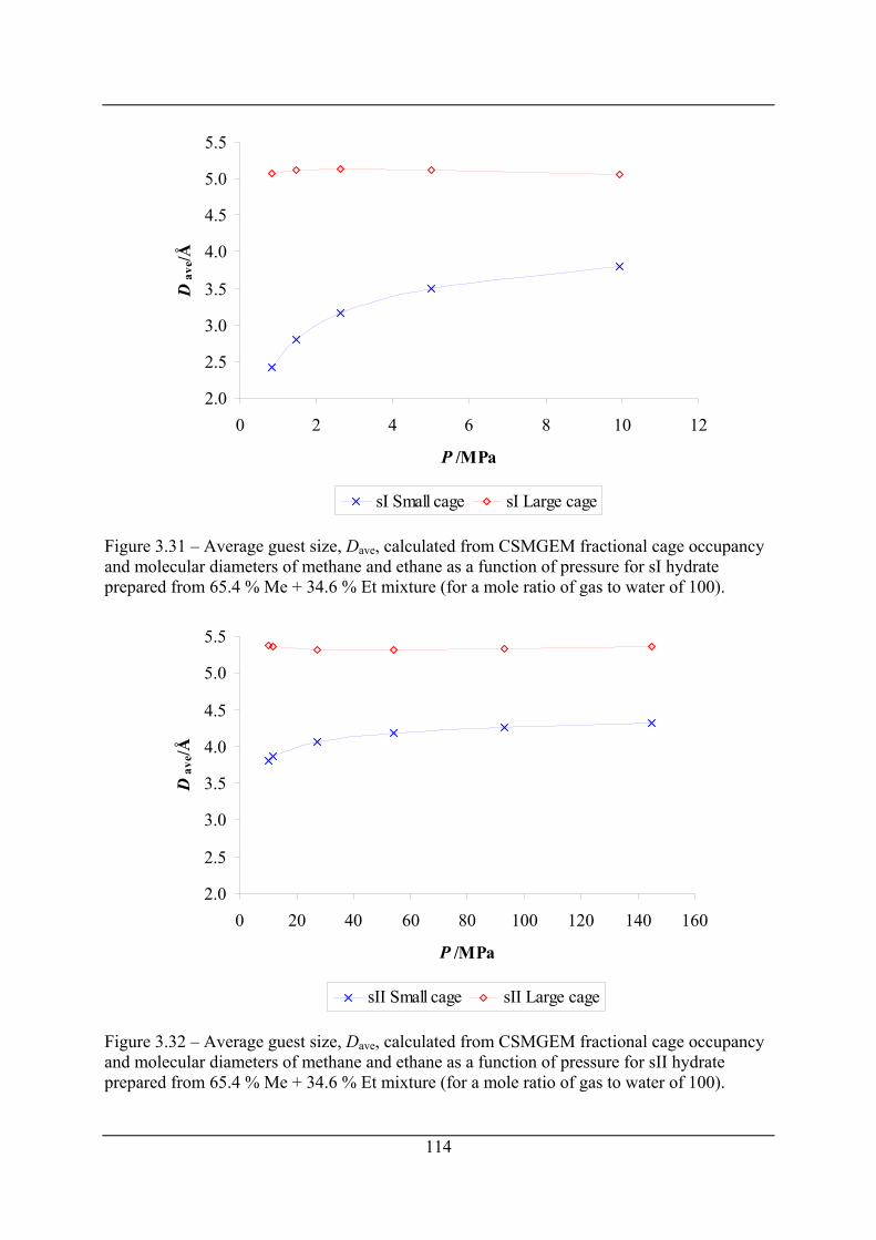
2.0
2.5
3.0
3.5
4.0
4.5
5.0
5.5
0 2 4 6 8 10 1
P /MPa
Dav
e/Å
2
sI Small cage sI Large cage
Figure 3.31 – Average guest size, Dave, calculated from CSMGEM fractional cage occupancy and molecular diameters of methane and ethane as a function of pressure for sI hydrate prepared from 65.4 % Me + 34.6 % Et mixture (for a mole ratio of gas to water of 100).
2.0
2.5
3.0
3.5
4.0
4.5
5.0
5.5
0 20 40 60 80 100 120 140 160
P /MPa
Dav
e/Å
sII Small cage sII Large cage
Figure 3.32 – Average guest size, Dave, calculated from CSMGEM fractional cage occupancy and molecular diameters of methane and ethane as a function of pressure for sII hydrate prepared from 65.4 % Me + 34.6 % Et mixture (for a mole ratio of gas to water of 100).
114
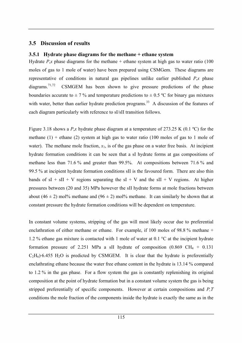
115
3.5 Discussion of results
3.5.1 Hydrate phase diagrams for the methane + ethane system Hydrate P,x phase diagrams for the methane + ethane system at high gas to water ratio (100
moles of gas to 1 mole of water) have been prepared using CSMGem. These diagrams are
representative of conditions in natural gas pipelines unlike earlier published P,x phase
diagrams.71,72 CSMGEM has been shown to give pressure predictions of the phase
boundaries accurate to ± 7 % and temperature predictions to ± 0.5 ºC for binary gas mixtures
with water, better than earlier hydrate prediction programs.33 A discussion of the features of
each diagram particularly with reference to sI/sII transition follows.
Figure 3.18 shows a P,x hydrate phase diagram at a temperature of 273.25 K (0.1 ºC) for the
methane (1) + ethane (2) system at high gas to water ratio (100 moles of gas to 1 mole of
water). The methane mole fraction, x1, is of the gas phase on a water free basis. At incipient
hydrate formation conditions it can be seen that a sI hydrate forms at gas compositions of
methane less than 71.6 % and greater than 99.5%. At compositions between 71.6 % and
99.5 % at incipient hydrate formation conditions sII is the favoured form. There are also thin
bands of sI + sII + V regions separating the sI + V and the sII + V regions. At higher
pressures between (20 and 35) MPa however the sII hydrate forms at mole fractions between
about (46 ± 2) mol% methane and (96 ± 2) mol% methane. It can similarly be shown that at
constant pressure the hydrate formation conditions will be dependent on temperature.
In constant volume systems, stripping of the gas will most likely occur due to preferential
enclathration of either methane or ethane. For example, if 100 moles of 98.8 % methane +
1.2 % ethane gas mixture is contacted with 1 mole of water at 0.1 °C at the incipient hydrate
formation pressure of 2.251 MPa a sII hydrate of composition (0.869 CH4 + 0.131
C2H6)·6.455 H2O is predicted by CSMGEM. It is clear that the hydrate is preferentially
enclathrating ethane because the water free ethane content in the hydrate is 13.14 % compared
to 1.2 % in the gas phase. For a flow system the gas is constantly replenishing its original
composition at the point of hydrate formation but in a constant volume system the gas is being
stripped preferentially of specific components. However at certain compositions and P,T
conditions the mole fraction of the components inside the hydrate is exactly the same as in the
116
gas phase. For example, a gas mixture of 70 % methane + 30 % ethane at P = 15.77 MPa and
T = 273.25 K is predicted to form a sII hydrate of composition (0.700 CH4 + 0.300
C2H6)·5.859 H2O. The dashed lines on Figure 3.18 represent the P,x conditions at which the
hydrate is predicted to enclathrate gas at the same mole fractions as the gas phase
composition. It can be shown however that these conditions are unstable. If the gas
composition is only slightly perturbed, divergent preferential enclathration will occur. This
can be illustrated about the point at 70 % methane + 30 % ethane at P = 15.77 MPa and T =
273.25 K. For a gas mixture of 69 % methane + 31 % ethane at the same pressure and
temperature the predicted hydrate has the composition (0.699 CH4 + 0.301 C2H6)·5.860 H2O.
The hydrate has a slight preference for methane in relation to its gas phase percentage and so
the gas phase methane composition will begin to drop (or x1 will decrease with hydrate
formation as shown in Figure 3.18). On the other hand for a gas mixture of 71 % methane +
29 % ethane the predicted hydrate composition is (0.702 CH4 + 0.298 C2H6)·5.857 H2O. The
hydrate has a slight preference for ethane in relation to it gas phase percentage and so the gas
phase ethane composition will begin to drop (or x1 will increase with hydrate formation as
shown in Figure 3.18). This concept is illustrated in Figure 3.18 with the arrows indicating
the direction that the gas phase will be stripped due to preferential enclathration.
Due to gas phase compositional changes during the hydrate formation process in the plug
formation cells, conditions that were initially believed would form sII plugs actually formed
sI plugs as shown by X-ray diffraction. Figure 3.19 shows the composition stripping
calculated for a pressure drop hydrate formation (see Chapter 4 for details of the models used
to calculate this stripping). The ethane rapidly becomes depleted due to its preferential
enclathration in the hydrate. For this reason gas mixtures containing approximately 80 %
methane + 20 % ethane were prepared in situ in the ISCO pump from pure methane and a
53 % methane + 46 % ethane mixture. Due to the stripping in a non-flow system this mixture
yielded sII hydrates close to the sI-sII phase boundary. Preferential enclathration is discussed
further in the next chapter.
The CSMGEM calculated P,T phase diagrams calculated at a high gas to water mole ratio
(100:1) presented for the 65.4 % methane + 34.6 % ethane mixture in Figure 3.20 and for the
98.8 % methane + 1.2 % ethane mixture in Figure 3.21 illustrate some interesting features.
117
Firstly comparing the P,T phase diagram for the 98.8 % methane + 1.2 % ethane mixture to
that for Bollavaram’s processed natural gas shown in Figure 3.4 both are clearly quite similar.
At lower pressure conditions sII hydrate is the stable structure and at high pressures sI is the
stable hydrate structure, the sI + sII + V boundary line/region also exhibits a similar negative
dP/dT slope. The P,T phase diagram for the 65.4 % methane + 34.6 % ethane mixture on the
other hand show some distinct differences with both that of the 98.8 % methane + 1.2 %
ethane mixture as well as Bollavaram’s processed natural gas. For this mixture sI hydrates
are the stable structure at lower hydrate formation pressures (up to 9.1 MPa incipient hydrate
formation conditions) and sII hydrates are the stable structure at higher pressures, the opposite
to the 98.8 % methane + 1.2 % ethane mixture and Bollavaram’s processed natural gas. Also
the slope of the sI + sII + V boundary line/region also exhibits an opposite positive dP/dT
slope.
CSMGEM calculated P,T phase predictions for pure methane sI hydrate were also plotted on
Figure 3.21 of the 98.8 % methane + 1.2 % ethane mixture. The H + Aq + V and H + I + V
lines for the sI region of the diagram for the mixture show close alignment with the data for
methane sI hydrate. The close alignment in Figure 3.21B suggests very similar dissociation
enthalpies for sI hydrates of this mixtures and sI methane hydrates as the Clapeyron equation
slope, dlnP/d(1/T), will be similar.
3.5.2 Plug dissociation Peters49 model for two-sided hydrate dissociation, the basis for plug dissociation prediction
package CSMPlug, suggests that the structure of hydrate has a strong effect on the
dissociation time. The model predicts that the dissociation of a sII plug will take
approximately 30 % longer than for a sI plug. If the dissociation temperature of the hydrate is
below the ice point the dissociated water will often freeze to form an ice plug even when
ambient conditions higher than the ice point. Taking this into account the model predicts that
removal of a hydrate and ice will take about 20 % longer for the sII plug than the sI plug.
Discussion of hydrate plug dissociation times with respect to structure follows.
A hydrate plug dissociation gas evolution plot for a predicted sI plug made from the gas
mixture of 65.4 % methane and 34.6 % ethane at CSM is shown in Figure 3.22. The plot
118
shows that the total time for conversion was about 42 min. CSMPlug predicted a similar
dissociation time of 40 min. By comparison of the actual hydrate number to the hydrate
number predicted using CSMGEM the conversion to hydrate was calculated to be 100 %.
A hydrate from the 65.4 % methane + 34.6 % ethane mixture was also prepared at higher
pressure. Figure 3.24 shows its phase diagram with the formation pressure/composition line.
The structure of this hydrate was confirmed by Raman spectrometry. Figure 3.26 shows the
vibrational spectra recorded for this hydrate. C-H and C-C vibrational frequencies for ethane
in the large cages of structures sI and sII have been compared to literature data at 274 K.36,71,94
The Raman spectra were taken at 77 K (-196 °C). By comparing the ethane peaks it is
possible to observe that the structure is sII (note there is a small shift to lower frequencies due
to the lower temperature of measurements). The lower ethane C-H vibration of 2883.0 cm-1 at
77 K is comparable to the 2887.3 cm-1 peak for sII at 274 K. The higher ethane C-H vibration
of 2939.0 cm-1 at 77 K is also comparable to the 2942.3 cm-1 peak for sII at 274 K.72 The C-C
stretch for the ethane at 77 K is the most comparable however, 992.0 cm-1 compared to the
992.9 cm-1 peak for sII at 274 K. It appears that this peak changes much less with
temperature.
The dissociation plot for the sII hydrate is shown in Figure 3.23. The experimental end time
was about 32 min compared to the CSMPlug prediction of 46.5 min. The CSMPlug
prediction is about 45 % greater than the experimental time which is larger than all the other
differences thus far. The sII forming Qatar gas used in Peters’ experiments49 also yielded a
shorter experimental dissociation time than predicted. Peter’s sI methane hydrate dissociation
showed agreement within about 15 % whereas from the sII the prediction was 120 % longer
than the experimental time. Peters suggested that sII dissociation may rely more on kinetic
effects. Due to the fact that the sII plug for the 65.4 % methane + 34.6 % ethane mixture had
to be formed at a higher pressure than that of the sI plug, its relative stability at atmospheric
pressure would be expected to be lower. Estimations of the enthalpy of dissociation by the
Clapeyron equation using CSMGem phase data indicate that the dissociation enthalpy is
higher for a sI than sII hydrate made from this mixture, whereas the opposite is true for the
98.8 % methane + 1.2 % methane mixture. A plot of the Clapeyron equation enthalpy of
dissociation estimates for hydrates formed from pure methane (sI), 65.4 mol% methane + 34.6
119
mol% ethane (sI and sII) and 98.8 % methane + 1.2 % ethane (sII) with pressure is included
as Figure 3.30 (note: more discussion on the Clapeyron equation estimates can be found in
section 3.5.3 of this chapter). These experimental results from the lower methane
composition structural transition region do not support the prediction that sII hydrates take
longer to dissociate. The results of Davies et al.40 appear at first to somewhat disagree with
this result. Davies et al. prepared sII hydrate plugs using a 65 % methane + 35 % ethane
mixture and compared the dissociation times to sI hydrate plugs formed with pure methane.
They found that the sII plugs took longer to dissociate than the sI plugs. The difference with
their measurements however was that they used pure methane to form their sI hydrates instead
of the 65 % methane + 35 % ethane mixture. Clapeyron equation calculations of the
enthalpies of dissociation using eqs (3.15) and (3.17) shown in Figure 3.30 suggest that the
methane sI hydrates have a lower enthalpy of dissociation than sII hydrates prepared from a
65.4 % methane + 34.6 % ethane mixture. However for natural gas systems the more
important structural transition region is at the high methane mole fraction transition. In this
case the Clapeyron equation calculations suggest that the enthalpy of dissociation of sII
98.8 % methane + 1.2 % ethane hydrate is higher than that of a sI pure methane hydrate.
Given that CSMPlug assumes a fixed value of the enthalpy of dissociation of sII hydrate
(640 kJ·kg-1) which is greater than the fixed value assumed for sI (460.24 kJ·kg-1)40, the
method which is used in the model is not in anyway invalidated by the above results. The
predictions from CSMPlug however should only be applied to hydrates formed from gas
mixtures with high methane mole fractions with the currently assumed values of enthalpies of
dissociation.
Seven hydrate plugs were prepared and dissociated to investigate the high methane structural
transition region at the University of Canterbury. The sI plugs were prepared from the 98.8 %
methane + 1.2 % ethane gas mixture. The sII plugs were prepared from 80 % methane +
20 % ethane mixtures prepared in situ using the ISCO pump. A further hydrate plug prepared
by the pressure drop (pressurized to approximately 8 MPa each pressurization) from the
98.8 % methane + 1.2 % ethane mixture showed evidence of containing both sI and sII
hydrates. The dissociation plot for this hydrate is shown in Figure 3.28 and appears to show
two distinct regions of dissociation. A hydrate formed from this gas at high gas to water ratio
is predicted to be sII by CSMGem, however due to non-flow preferential enclathration of the
120
ethane the gas is likely to be stripped to virtually pure methane and most of the plug was
likely sI. Due to this particular plug being the least porous (ε = 0.462) it is hypothesized that
gas mixing along the length of the ice/hydrate plug during formation was more highly
impeded than for other plugs and gas diffusion would be slower through the plug. This meant
that the ends of the plug may have stripped out all the ethane to form sII hydrates before any
of the ethane could reach the middle of the plug. This would lead to disks or cylindrical
sections of sII hydrate at either end of the plug. If it is assumed as predicted that sI
dissociates more quickly the gas evolution curve would be expected to be dominated by
evolution from the sI section of the hydrate for the first time period. As gas evolution from
the sI section tailed off the sII gas evolution would be at a faster rate than that from the sI
section and the sII section would dominate the final dissociation time. This evolution plot
would appear to show this behaviour with a distinct change in gas evolution rate at just after
40 min. The hydrate dissociation time for this plug has been assumed to be effectively a sII
hydrate dissociation time because it appears that the sII hydrate controls the final time. None
of the other plugs prepared from the 98.8 % methane + 1.2 % ethane mixture appeared to
show two distinct regions of dissociation.
Figure 3.25 shows a plot of the experimental and the predicted hydrate dissociations times
versus the hydrate porosity (the void fraction of the plug). The porosity value is the likely
greatest source of experimental-model discrepancy. The porosity was estimated from the
mass of ice particles, the volume of the cell and a hydrate density calculated using CSMGem.
Although the cell was tapped with a mallet around the thermowells there may have been areas
devoid of ice particles. Also as the cell was loaded with ice particles vertically there may
have be a segregation of the smaller particles towards the bottom of the cell. These two
affects could have caused significant errors in the calculated porosity. The overall conversion
of all of the plugs was 97 % or greater. Table 3.6 shows the experimental and CSMPlug
predicted dissociation times. The percentage difference the CSMPlug prediction is from the
experimental value is also tabulated. The percentage difference of the model prediction from
the experimental time for sI plugs spans from -2 % to +20 % giving a mean of – 2.4 %. For
the sII plug this difference spans from +3 % to +14 % giving a mean of +8%. The model
predicts that the sII plugs will take from 38 % to 40 % longer to dissociate. Applying the two
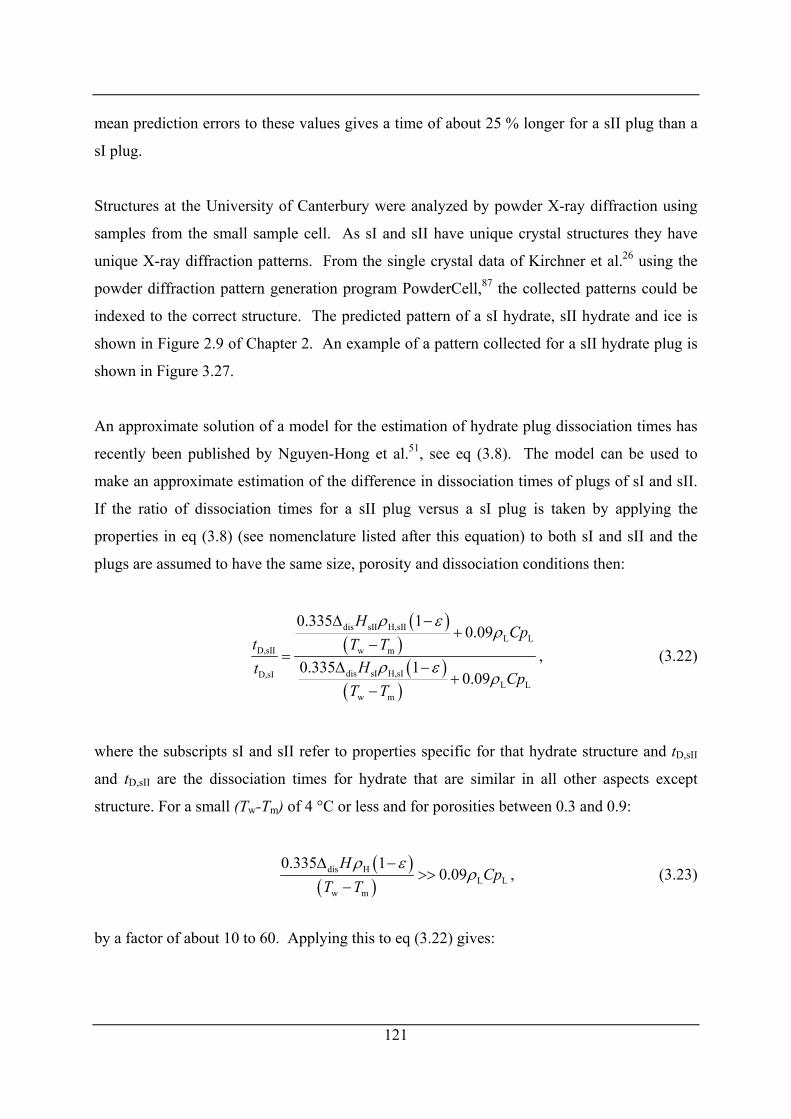
mean prediction errors to these values gives a time of about 25 % longer for a sII plug than a
sI plug.
Structures at the University of Canterbury were analyzed by powder X-ray diffraction using
samples from the small sample cell. As sI and sII have unique crystal structures they have
unique X-ray diffraction patterns. From the single crystal data of Kirchner et al.26 using the
powder diffraction pattern generation program PowderCell,87 the collected patterns could be
indexed to the correct structure. The predicted pattern of a sI hydrate, sII hydrate and ice is
shown in Figure 2.9 of Chapter 2. An example of a pattern collected for a sII hydrate plug is
shown in Figure 3.27.
An approximate solution of a model for the estimation of hydrate plug dissociation times has
recently been published by Nguyen-Hong et al.51, see eq (3.8). The model can be used to
make an approximate estimation of the difference in dissociation times of plugs of sI and sII.
If the ratio of dissociation times for a sII plug versus a sI plug is taken by applying the
properties in eq (3.8) (see nomenclature listed after this equation) to both sI and sII and the
plugs are assumed to have the same size, porosity and dissociation conditions then:
( )( )
( )( )
dis sII H,sIIL L
D,sII w m
dis sI H,sID,sIL L
w m
0.335 10.09
0.335 10.09
HCp
t T THt Cp
T T
ρ ερ
ρ ερ
Δ −+
−=
Δ −+
−
, (3.22)
where the subscripts sI and sII refer to properties specific for that hydrate structure and tD,sII
and tD,sII are the dissociation times for hydrate that are similar in all other aspects except
structure. For a small (Tw-Tm) of 4 °C or less and for porosities between 0.3 and 0.9:
( )( )
dis HL L
w m
0.335 10.09
HCp
T Tρ ε
ρΔ −
>>−
, (3.23)
by a factor of about 10 to 60. Applying this to eq (3.22) gives:
121
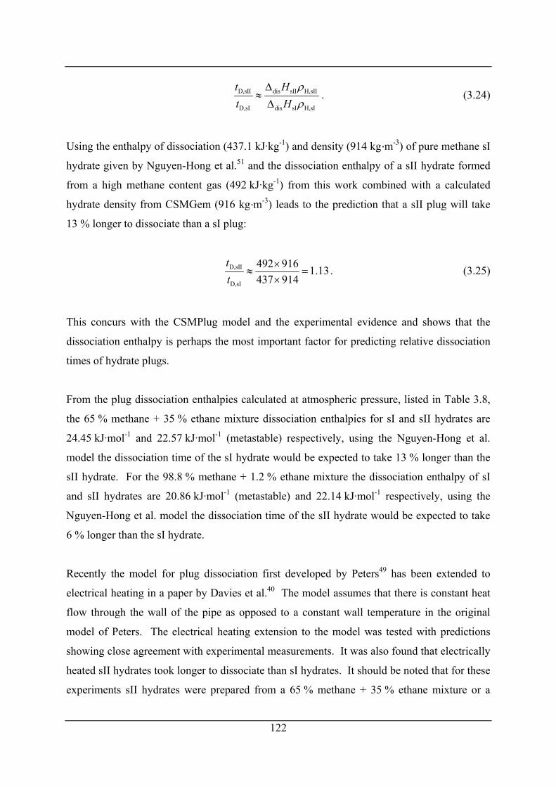
D,sII dis sII H,sII
D,sI dis sI H,sI
t Ht H
ρρ
Δ≈Δ
. (3.24)
Using the enthalpy of dissociation (437.1 kJ·kg-1) and density (914 kg·m-3) of pure methane sI
hydrate given by Nguyen-Hong et al.51 and the dissociation enthalpy of a sII hydrate formed
from a high methane content gas (492 kJ·kg-1) from this work combined with a calculated
hydrate density from CSMGem (916 kg·m-3) leads to the prediction that a sII plug will take
13 % longer to dissociate than a sI plug:
D,sII
D,sI
492 916 1.13437 914
tt
×≈ =
×. (3.25)
This concurs with the CSMPlug model and the experimental evidence and shows that the
dissociation enthalpy is perhaps the most important factor for predicting relative dissociation
times of hydrate plugs.
From the plug dissociation enthalpies calculated at atmospheric pressure, listed in Table 3.8,
the 65 % methane + 35 % ethane mixture dissociation enthalpies for sI and sII hydrates are
24.45 kJ·mol-1 and 22.57 kJ·mol-1 (metastable) respectively, using the Nguyen-Hong et al.
model the dissociation time of the sI hydrate would be expected to take 13 % longer than the
sII hydrate. For the 98.8 % methane + 1.2 % ethane mixture the dissociation enthalpy of sI
and sII hydrates are 20.86 kJ·mol-1 (metastable) and 22.14 kJ·mol-1 respectively, using the
Nguyen-Hong et al. model the dissociation time of the sII hydrate would be expected to take
6 % longer than the sI hydrate.
Recently the model for plug dissociation first developed by Peters49 has been extended to
electrical heating in a paper by Davies et al.40 The model assumes that there is constant heat
flow through the wall of the pipe as opposed to a constant wall temperature in the original
model of Peters. The electrical heating extension to the model was tested with predictions
showing close agreement with experimental measurements. It was also found that electrically
heated sII hydrates took longer to dissociate than sI hydrates. It should be noted that for these
experiments sII hydrates were prepared from a 65 % methane + 35 % ethane mixture or a
122
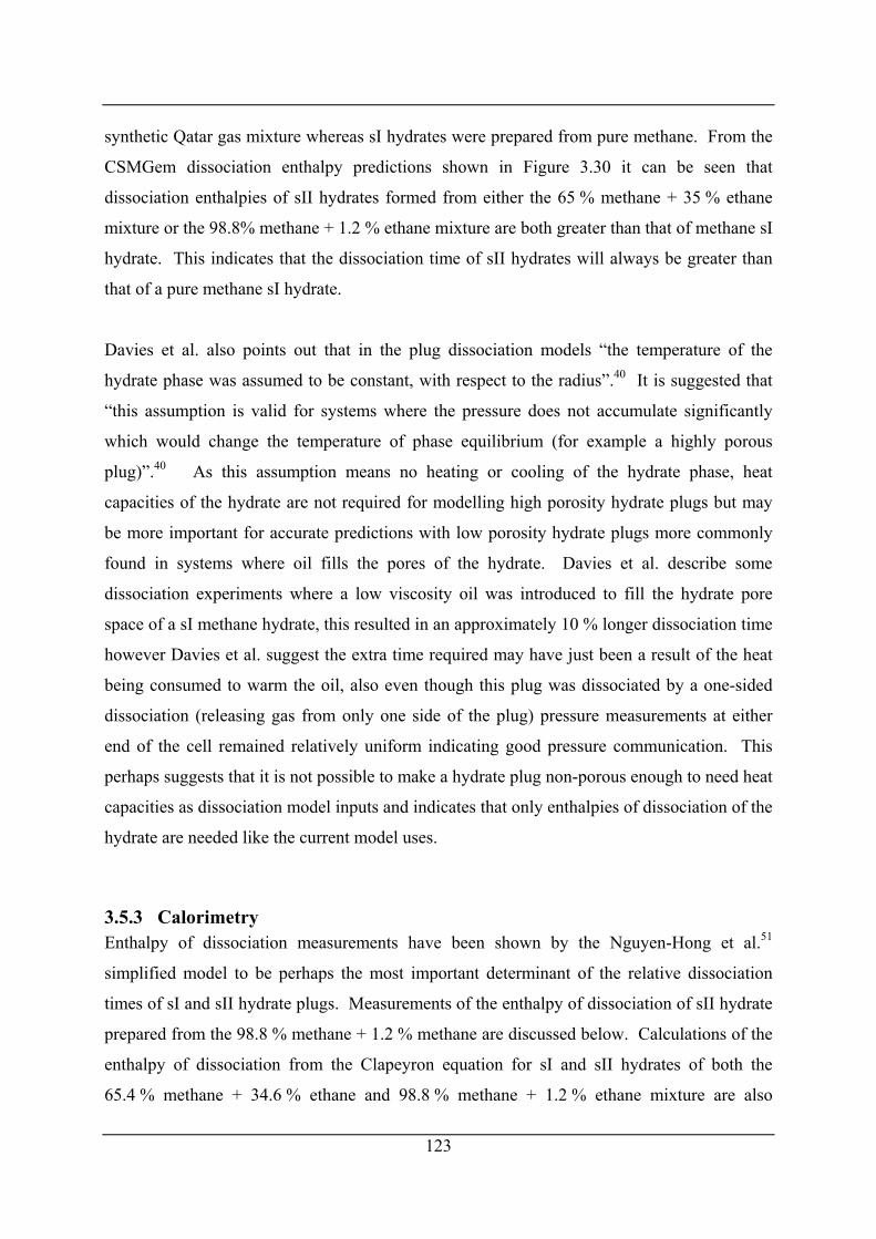
123
synthetic Qatar gas mixture whereas sI hydrates were prepared from pure methane. From the
CSMGem dissociation enthalpy predictions shown in Figure 3.30 it can be seen that
dissociation enthalpies of sII hydrates formed from either the 65 % methane + 35 % ethane
mixture or the 98.8% methane + 1.2 % ethane mixture are both greater than that of methane sI
hydrate. This indicates that the dissociation time of sII hydrates will always be greater than
that of a pure methane sI hydrate.
Davies et al. also points out that in the plug dissociation models “the temperature of the
hydrate phase was assumed to be constant, with respect to the radius”.40 It is suggested that
“this assumption is valid for systems where the pressure does not accumulate significantly
which would change the temperature of phase equilibrium (for example a highly porous
plug)”.40 As this assumption means no heating or cooling of the hydrate phase, heat
capacities of the hydrate are not required for modelling high porosity hydrate plugs but may
be more important for accurate predictions with low porosity hydrate plugs more commonly
found in systems where oil fills the pores of the hydrate. Davies et al. describe some
dissociation experiments where a low viscosity oil was introduced to fill the hydrate pore
space of a sI methane hydrate, this resulted in an approximately 10 % longer dissociation time
however Davies et al. suggest the extra time required may have just been a result of the heat
being consumed to warm the oil, also even though this plug was dissociated by a one-sided
dissociation (releasing gas from only one side of the plug) pressure measurements at either
end of the cell remained relatively uniform indicating good pressure communication. This
perhaps suggests that it is not possible to make a hydrate plug non-porous enough to need heat
capacities as dissociation model inputs and indicates that only enthalpies of dissociation of the
hydrate are needed like the current model uses.
3.5.3 Calorimetry Enthalpy of dissociation measurements have been shown by the Nguyen-Hong et al.51
simplified model to be perhaps the most important determinant of the relative dissociation
times of sI and sII hydrate plugs. Measurements of the enthalpy of dissociation of sII hydrate
prepared from the 98.8 % methane + 1.2 % methane are discussed below. Calculations of the
enthalpy of dissociation from the Clapeyron equation for sI and sII hydrates of both the
65.4 % methane + 34.6 % ethane and 98.8 % methane + 1.2 % ethane mixture are also
discussed. The enthalpy of dissociation is also considered in terms of the average predicted
guest size of the each cage of each structure for the 65.4 % methane + 34.6 % ethane mixture.
Measurements of the enthalpy of dissociation of sII hydrate with the 98.8 % methane + 1.2 %
ethane gas mixture have been completed using the DSC at a pressure of about 7 MPa. The
results of the dissociation enthalpy measurements are recorded in Table 3.7. The first
measurement of (66.47 ± 0.50) kJ·mol-1 at a pressure of 7.03 MPa was conducted with hydrate
formed inside the calorimeter by the method first used by Marsh and Gao.143 The second
measurement of (63.15 ± 0.50) kJ·mol-1 at a pressure of 6.92 MPa was made from
cryogenically transferred hydrate. The conversion to hydrate for the second measurement was
98.16 % compared to 64.26 % for the first. Higher conversions are usually considered to
result in better measurements of the dissociation enthalpy.143 Figure 3.29 shows the pre-
hydrate dissociation ice peak, the hydrate dissociation ice peak as well as the post-hydrate
dissociation ice peak for the second measurement. The two different hydrates may have had
slightly different hydrate compositions due to their different methods of preparation, this may
explain why the 3.32 kJ·mol-1 difference in dissociation enthalpies despite the close
dissociation pressures.
A comparison of the measured values to predictions of the enthalpy of hydrate dissociation is
also given in Table 3.7. The predicted values were calculated from CSMGem P,T phase
stability data and compressibility factors (calculated from molecular masses, mass densities,
P, R and T). Calculations using the compressibility factor difference expressed by eq (3.17)
as well as GZ ZΔ = − where completed using the Clapeyron equation as expressed by eq
(3.15). Traditionally it has been assumed that the compressibility factor of the gas, ZG, is the
dominant term (the compressibility factor of the water and the hydrate are assumed
negligible) as represented by GZ ZΔ = . The compressibility difference represented by
equation eq (3.17) is equivalent mathematically to the molar volume difference that
Anderson156 used for his study of the enthalpy of dissociation of methane hydrate except it
has been assumed that the gases are not soluble in the aqueous phase.
Gupta50 has recently measured the enthalpy of dissociation of sI methane hydrate up to 20
MPa and found that above about 10 MPa that, unless the water and hydrate phase
124
compressibility were taken into account, errors in the dissociation enthalpy predicted using
the Clapeyron equation would be in the range of (50 to 100) % (see Figure 3.12 taken from
Gupta). By comparing Anderson’s156 molar volume differences to the molar volume of pure
methane the difference in enthalpies of dissociation from the use of this expression versus
using only the gas molar volume can be calculated. Similarly to what Gupta found it can be
shown that at 9.88 MPa there is a 30 % difference by using the molar volume difference
rather than only the molar volume of the gas ( GV VΔ = ). This difference grows almost
linearly with pressure, exceeding 100 % (124 %) at 69.68 MPa and higher pressures. The
prediction using the eq (3.17) form of ΔZ is only 0.9 % higher than the experimental value for
the 98.16 % hydrate compared to a 10 % lower value from GZ ZΔ = . This suggests that more
accurate predictions of enthalpies of hydrate formation can be made using the eq (3.17) ΔZ.
Considering the accuracy of the phase prediction data and the compressibility factors as the
only sources of error for use in the Clapeyron equation these values are estimated to have an
uncertainty of ± 4.5 %.
The hydrate formation enthalpy for pure methane hydrate of 54.19 kJ·mol-1 from Handa,135 is
about 18 % lower than the value measured for the sII hydrate. The higher formation enthalpy
would suggest that the dissociation time would be longer for the sII hydrate because more
energy would be required to dissociate it.
Given that the structural transition is at such a high methane composition it has been assumed
that the enthalpy of dissociation for a sI hydrate prepared from a high methane gas mixture
would be the same as that of a pure methane sI hydrate. The P,T phase diagrams shown in
Figure 3.21 for the 98.8 % methane + 1.2 % ethane mixture are overlaid with data for
methane sI hydrate. The methane hydrate lines and the sI lines for the mixture are very
closely aligned, the similar Clapeyron equation slopes (dlnP/d(1/T)) in part (B) of the figure
indicate very similar dissociation enthalpies given that the small fraction of ethane in the gas
and hydrate will have little effect on their compressibility factors.
The Clapeyron equation with P,T phase data and compressibilites for each phase (calculated
from molar masses, mass densities, P, R and T) from CSMGem predictions was used to
estimate the dissociation enthalpy of hydrates prepared from the 65.4 % methane + 34.6 %
125
126
ethane mixture (sI and sII), the 98.8 % methane + 1.2 % ethane mixture (sII) and 100 %
methane (sI). Error in the values has been estimated at 4.5 % from the error in the P,T phase
data and compressibilites from CSMGem. The calculated dissociation enthalpies as well as
the experimental measurements were plotted with pressure in Figure 3.30. The estimations
suggest that for high methane natural gases the dissociation enthalpies for sII hydrates
(represented by the 98.8 % methane + 1.2 % ethane mixture sII data) are higher than those of
sI hydrates (represented by the pure methane sI hydrate data). The estimation also shows that
the case is the opposite for the 65.4 % methane + 35 % ethane hydrates (the sII hydrates have
lower dissociation enthalpies than the sI hydrates). For comparison with the plug dissociation
time measurements of Davies et al40 it can be seen that the estimated dissociation enthalpies
of the 65.4 % methane + 34.6 % ethane sII hydrates are higher than those of pure methane sI
hydrates. Although several authors suggest that the Clapeyron equation can only be used at
univariant conditions,148,150 comparison of the predicted hydrate dissociation enthalpies seem
to be within reasonable agreement with the experimental value using the eq (3.17) form of
ΔZ, deviating by 0.8 % at 6.92 MPa and 5.9 % at 7.03 MPa. It is also interesting to note that,
in comparison that the methane hydrate predictions are almost constant with pressure and are
within the range of calorimetric results reported in Table 3.2.
The change in the enthalpy with pressure (and hence temperature), particularly for the sI
hydrate formed from the 65 % methane + 35 % ethane mixture, is most likely a result of
changing guest size. Sloan and Fleyfel154,155 first suggested that larger guests resulted in
larger enthalpies of dissociation. Plots of the average guest size for the large and small cage
versus pressure for the 65 % methane + 35 % ethane sI and sII hydrates are shown in Figure
3.31 and Figure 3.32 respectively. It can be seen that the large cage guest for both hydrates
changes little with pressure, however that of the small cage changes more significantly. The
small cage average guest size for the sI hydrate increases by about 1.4 Å over a pressure range
of about 9 MPa. For the sII hydrate the small cage average guest size only increases very
marginally by about 0.5 Å over a pressure range of about 135 MPa. The much larger change
in small guest average size in the sI hydrate would appear to give rise to the comparatively
much larger change in the calculated dissociation enthalpy with pressure/temperature.
127
3.5.4 Further calorimetric measurements Initially more measurements of enthalpies of dissociation of gas hydrates were planned as
well as measurement of heat capacities, however due to recurring breakdowns of the DSC
used in this work these measurements were not possible. Measurements of the enthalpies of
dissociation of sI and sII hydrates formed from the mixture of mole fractions 65.4 % methane
+ 34.6 % ethane would have been useful as further confirmation of Clapeyron equation
predictions presented in this chapter. From the literature review there is a general lack of
calorimetrically measured enthalpies of dissociation and heat capacity data for gas hydrates of
both pure gases and gas mixtures. Measurements of the enthalpies of dissociation of highly
soluble gaseous guests such as CO2 or H2S would be particularly useful to investigate
assumptions associated with the used of the Clapeyron equation.
128
Chapter 4 PREFERENTIAL ENCLATHRATION AND GAS PHASE STRIPPING DURING LABORATORY HYDRATE FORMATION FROM
GAS MIXTURES
4.1 Introduction In doing the plug dissociation studies in this work at high methane mole fractions a
discontinuity was observed in the gas evolution rate (see Figure 3.28) and X-ray diffraction
indicated the possibility of the presence of both sI and sII hydrate structures in some plugs.
Forming laboratory hydrate samples that are representative of hydrates encountered
industrially for plug dissociation and other studies is important if laboratory results are to be
applied to industry. It is of particularly importance in the case of plug dissociation studies
that the structure of the hydrate formed is that that was desired (or even in worst case
assumed). Typically this is not a problem when preparing a hydrate of a single guest
component as most single guests only form one structure of hydrate over a wide range of P,T
conditions. For mixtures of gases on the other hand it has been shown that changes in the
composition can result in the formation of hydrates of a different structure. One such mixture
is methane + ethane, even though both components form sI hydrate as single guests a mixture
of the two gases at certain compositions can result in the formation of sII hydrates,71,72 the
stable hydrate structure has also shown to be a function of the composition in multi-
component natural gas mixtures (see Chapter 3). Duplication of conditions such as the flow
of gas through or around ice or water when forming a hydrate is not always possible in the
laboratory, yet the industrial conditions where water or ice contact gas to form hydrate plugs
are under flow conditions (or conditions were there is a extremely large mole excess of gas to
water). The formation of hydrates in the laboratory are typically carried out under conditions
where the gas supplied to the ice or water for the formation to the hydrate is only just in
excess of that which is required for complete conversion of ice or water to hydrate.
Although hydrate phase stability predictions packages such as CSMGem can perform
simulations and predict conditions where only sI, only sII or a mixture of sI and sII hydrates
form under excess water conditions, such as that shown for a mixture of methane + ethane on
the isothermal P,x diagram of Figure 3.1, these prediction packages don’t explain why (or
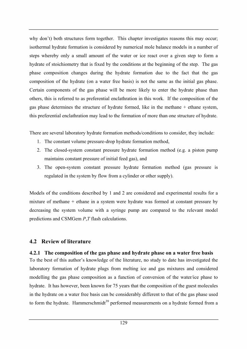
129
why don’t) both structures form together. This chapter investigates reasons this may occur;
isothermal hydrate formation is considered by numerical mole balance models in a number of
steps whereby only a small amount of the water or ice react over a given step to form a
hydrate of stoichiometry that is fixed by the conditions at the beginning of the step. The gas
phase composition changes during the hydrate formation due to the fact that the gas
composition of the hydrate (on a water free basis) is not the same as the initial gas phase.
Certain components of the gas phase will be more likely to enter the hydrate phase than
others, this is referred to as preferential enclathration in this work. If the composition of the
gas phase determines the structure of hydrate formed, like in the methane + ethane system,
this preferential enclathration may lead to the formation of more than one structure of hydrate.
There are several laboratory hydrate formation methods/conditions to consider, they include:
1. The constant volume pressure-drop hydrate formation method,
2. The closed-system constant pressure hydrate formation method (e.g. a piston pump
maintains constant pressure of initial feed gas), and
3. The open-system constant pressure hydrate formation method (gas pressure is
regulated in the system by flow from a cylinder or other supply).
Models of the conditions described by 1 and 2 are considered and experimental results for a
mixture of methane + ethane in a system were hydrate was formed at constant pressure by
decreasing the system volume with a syringe pump are compared to the relevant model
predictions and CSMGem P,T flash calculations.
4.2 Review of literature
4.2.1 The composition of the gas phase and hydrate phase on a water free basis To the best of this author’s knowledge of the literature, no study to date has investigated the
laboratory formation of hydrate plugs from melting ice and gas mixtures and considered
modelling the gas phase composition as a function of conversion of the water/ice phase to
hydrate. It has however, been known for 75 years that the composition of the guest molecules
in the hydrate on a water free basis can be considerably different to that of the gas phase used
to form the hydrate. Hammerschmidt39 performed measurements on a hydrate formed from a
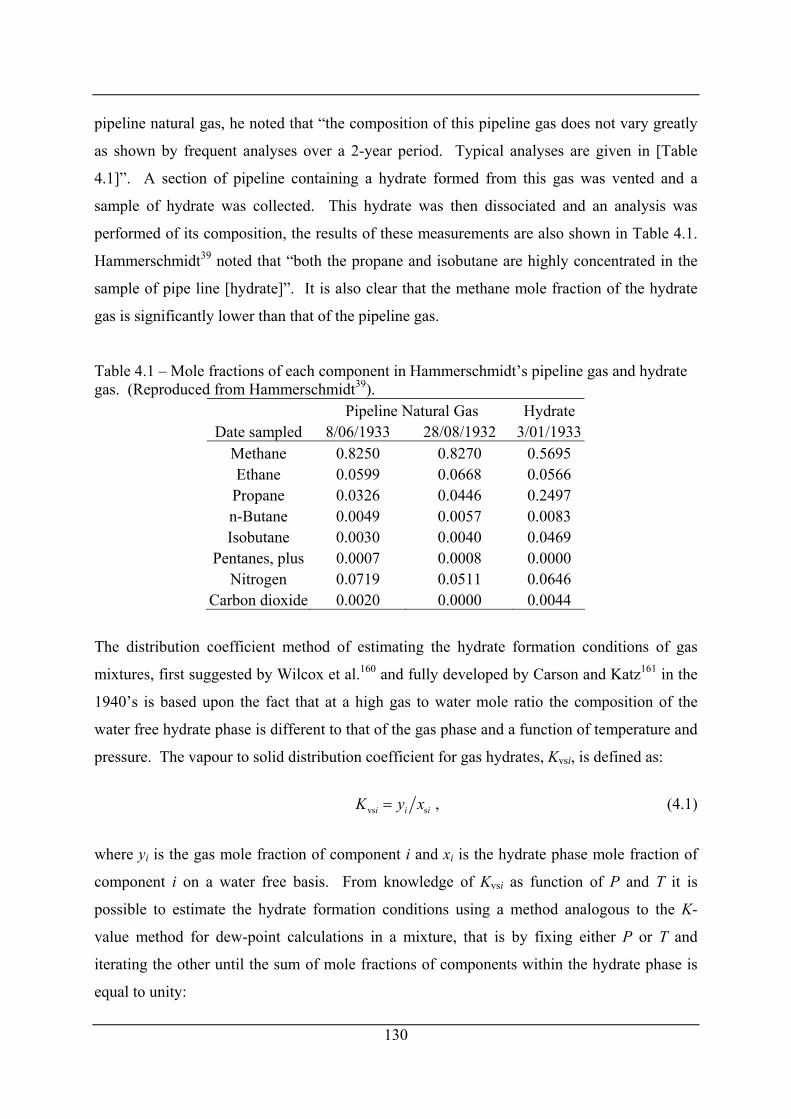
pipeline natural gas, he noted that “the composition of this pipeline gas does not vary greatly
as shown by frequent analyses over a 2-year period. Typical analyses are given in [Table
4.1]”. A section of pipeline containing a hydrate formed from this gas was vented and a
sample of hydrate was collected. This hydrate was then dissociated and an analysis was
performed of its composition, the results of these measurements are also shown in Table 4.1.
Hammerschmidt39 noted that “both the propane and isobutane are highly concentrated in the
sample of pipe line [hydrate]”. It is also clear that the methane mole fraction of the hydrate
gas is significantly lower than that of the pipeline gas.
Table 4.1 – Mole fractions of each component in Hammerschmidt’s pipeline gas and hydrate gas. (Reproduced from Hammerschmidt39).
Pipeline Natural Gas Hydrate Date sampled 8/06/1933 28/08/1932 3/01/1933
Methane 0.8250 0.8270 0.5695 Ethane 0.0599 0.0668 0.0566
Propane 0.0326 0.0446 0.2497 n-Butane 0.0049 0.0057 0.0083 Isobutane 0.0030 0.0040 0.0469
Pentanes, plus 0.0007 0.0008 0.0000 Nitrogen 0.0719 0.0511 0.0646
Carbon dioxide 0.0020 0.0000 0.0044
The distribution coefficient method of estimating the hydrate formation conditions of gas
mixtures, first suggested by Wilcox et al.160 and fully developed by Carson and Katz161 in the
1940’s is based upon the fact that at a high gas to water mole ratio the composition of the
water free hydrate phase is different to that of the gas phase and a function of temperature and
pressure. The vapour to solid distribution coefficient for gas hydrates, Kvsi, is defined as:
vs si iK y x i= , (4.1)
where yi is the gas mole fraction of component i and xi is the hydrate phase mole fraction of
component i on a water free basis. From knowledge of Kvsi as function of P and T it is
possible to estimate the hydrate formation conditions using a method analogous to the K-
value method for dew-point calculations in a mixture, that is by fixing either P or T and
iterating the other until the sum of mole fractions of components within the hydrate phase is
equal to unity:
130
1 vs
1n
i
i i
yK=
=∑ , (4.2)
where n is the total number of components in the gas mixture. Carson and Katz161 set values
for the Kvsi for methane as a function of P and T and values for other component were derived
from two component gas mixtures based on the values of methane (Carson and Katz produced
charts of Kvsi as a function of P and T for ethane and propane, other authors produced charts
for further components, see Sloan and Koh2 section 4.2.2 for charts, Kvsi correlations with T
and P and references, note: Kvsi were based on methane in mixtures that form sII hydrates). It
is clear that because the values of Kvsi are functions of temperature and pressure for individual
components that hydrate gas compositions on a water free basis can be very different to that
of the gas surrounding the hydrate and the success of this method’s prediction of hydrate
formation P,T conditions is based upon this fact. The absolute average deviation of pressure
predictions for a given temperature using the Kvsi values has been evaluated from data from 20
natural gases, the deviation was 12.3 % compared to 5.8 % for CSMGem.2
The model of van der Waals and Platteeuw32 described briefly in the introduction calculates
the composition of the hydrate based on fractional occupancies calculated from Langmuir
adsorption constants derived from statistical thermodynamics. This model provides a way of
calculating the hydrate phase composition from the P, T and composition of the gas.
CSMGem (developed by Ballard33) further allows flash calculations in the hydrate region at
pressures higher than the incipient pressure or lower temperatures than the dissociation
temperature and hence allows for the calculation of more than an infinitely small amount of
the hydrate phase. This means that the effect of the ratio of moles of water to gas can be
investigated (note: sometimes however the program does not always converge to a solution at
high mole ratios of water to gas).
The separation of gases has even been proposed and investigated, using the fact that the water
free gas composition of the hydrate phase is different to that of the gas. Happel et al.162
studied the separation of methane and nitrogen by the formation of hydrates in a continuous
flow reactor. A 1 L high pressure reactor, with jacketed temperature control and a
magnetically coupled turbine agitator was used in experiments. The flow rate of gas mixtures
131
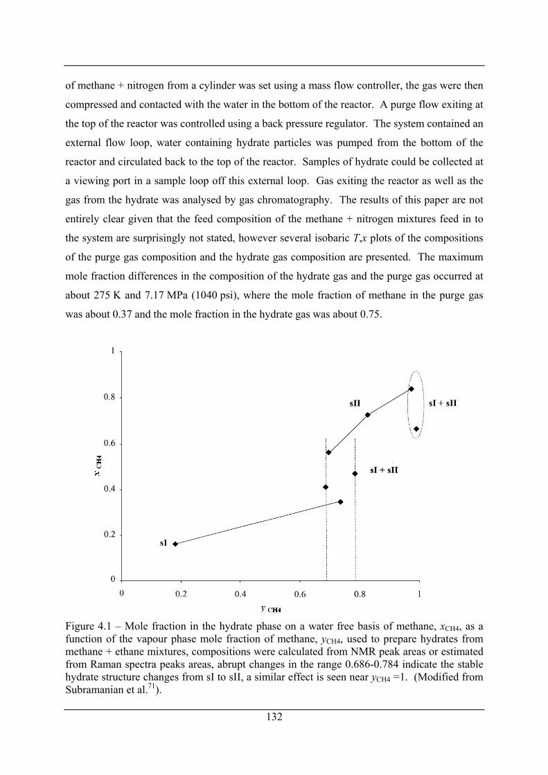
of methane + nitrogen from a cylinder was set using a mass flow controller, the gas were then
compressed and contacted with the water in the bottom of the reactor. A purge flow exiting at
the top of the reactor was controlled using a back pressure regulator. The system contained an
external flow loop, water containing hydrate particles was pumped from the bottom of the
reactor and circulated back to the top of the reactor. Samples of hydrate could be collected at
a viewing port in a sample loop off this external loop. Gas exiting the reactor as well as the
gas from the hydrate was analysed by gas chromatography. The results of this paper are not
entirely clear given that the feed composition of the methane + nitrogen mixtures feed in to
the system are surprisingly not stated, however several isobaric T,x plots of the compositions
of the purge gas composition and the hydrate gas composition are presented. The maximum
mole fraction differences in the composition of the hydrate gas and the purge gas occurred at
about 275 K and 7.17 MPa (1040 psi), where the mole fraction of methane in the purge gas
was about 0.37 and the mole fraction in the hydrate gas was about 0.75.
Figure 4.1 – Mole fraction in the hydrate phase on a water free basis of methane, xCH4, as a function of the vapour phase mole fraction of methane, yCH4, used to prepare hydrates from methane + ethane mixtures, compositions were calculated from NMR peak areas or estimated from Raman spectra peaks areas, abrupt changes in the range 0.686-0.784 indicate the stable hydrate structure changes from sI to sII, a similar effect is seen near yCH4 =1. (Modified from Subramanian et al.71).
132
133
Studies of hydrates formed from methane + ethane mixtures by Subramanian et al.72 and
Kini163 reveal the mole fraction of methane and ethane in the hydrate phase as a function of
vapour phase mole fractions used to form the hydrates. The mole fractions of methane and
ethane in the vapour phase and the hydrate phases were calculated from NMR peak areas or
Raman spectra peak areas (Note: the Raman peak areas could be used to estimate the
composition of methane + ethane mixtures as a calibration curve of the ratio of methane to
ethane Raman peak areas versus the methane to ethane mole ratio of calibration gases of
known mole fractions had been prepared, see Subramanian et al.72). A step change was
observed in the hydrate phase composition for hydrates prepared from the methane + ethane
mixture with a mole fraction of methane in the gas mixture of between 0.7 and 0.8, this is
illustrated in Figure 4.1 reproduced from Subramanian et al.71 The change was attributed to a
change in the structure of hydrate formed from the mixture of sI to sII, a similar but opposite
change from sII to sI was observed between methane mole fractions in the vapour phase of
about (0.97 and 0.99). The upper transition point was determined more accurately by Raman
spectroscopy to occur between methane mole fractions in the vapour phase of (0.992 to
0.994). These results showed that the composition of the vapour phase is crucial in the
determination of the structure of hydrate that will form.
4.2.2 Notes on metastability Several authors have conducted experimental studies which have shown that usual sI hydrate
formers carbon dioxide164,165 and methane166 can transiently form metastable sII crystals. A
recent article also showed evidence of formation of both sI and sII hydrate for mixtures of
methane + ethane + propane hydrates.167 In this study hydrates were formed under flow
conditions or conditions of a large volume of gas to water. It was determined by the authors
that these conditions would result in no or limited changes in the gas composition so that the
formation of a different structures due to composition changes in the gas was not a
contributing cause. Four different mixtures were investigated with mole fractions between
(90.28 and 98.01) % methane, between (0 and 4.95) % ethane and between (0.65 and 4.77) %
propane. For all of the mixtures morphological changes were observed when crystals of
hydrate formed just below the three phase H + Aq + V line were cooled isobarically to
temperatures below the H + Aq + V line of pure methane hydrate. Large euhedral crystal
transitioned to a fine crystal foamy mass. A reversal in morphology could be achieved by
134
reheating above the H + Aq + V line of pure methane hydrate. “Raman spectroscopy and X-
ray diffraction data indicated that formation/decomposition of sI methane hydrates was part of
this process”.167
The models in this study do not investigate metastability, the most stable hydrate predicted
using CSMGem is assumed to be formed given a composition of gas and the temperature and
pressure.
4.3 Models and calculations
4.3.1 The extremes of hydrate formation and preferential enclathration Consider this thought experiment: A piston maintained at constant temperature contains water
and a gas mixture (containing only components that can be enclathrated in hydrate cages) at a
ratio to which there is excess water in requirement to fully convert all of a gas mixture to
hydrate. If the piston is compressed so the conditions are within the hydrate formation P,T
region hydrate will begin to form until the pressure drops to the incipient pressure at the set
temperature. However if the mixture is continuously compressed by the piston to maintain
the conditions within the hydrate formation region then the gas will continue to combine with
remaining water until all the gas is consumed. It is then clear that the hydrate composition on
a water free basis on average will be equal to the initial gas mixture composition.
Alternatively the above piston can be considered for a system containing a very small amount
of water and a large amount of gas (in mole terms). If such a system is in the hydrate
formation P,T region then hydrate formation will occur to consume all the aqueous phase.
The hydrate composition under these conditions is defined by the measured Kvsi values
discussed in the introduction to this section. The hydrate composition on a water free basis
can be considerably different to the composition of the gas mixture (note: however under
certain conditions the hydrate composition on a water free basis can be the same as that of the
gas mixture, see the dashed lines on Figure 3.18 and refer to Section 3.4.1 for further detail).
To form a large hydrate plug in the laboratory ice particles are typically melted just above the
ice point temperature in a pressure cell in the presence of a hydrate forming gas above the
hydrate formation incipient pressure, this method was developed by Stern et al.126 and is
discussed in detail in Chapter 3 of this work. The amount of gas feed to the known amount of
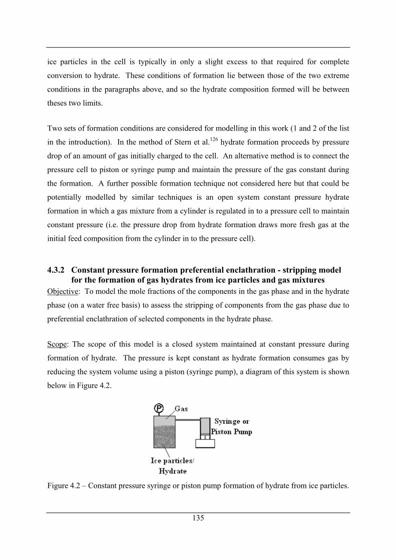
ice particles in the cell is typically in only a slight excess to that required for complete
conversion to hydrate. These conditions of formation lie between those of the two extreme
conditions in the paragraphs above, and so the hydrate composition formed will be between
theses two limits.
Two sets of formation conditions are considered for modelling in this work (1 and 2 of the list
in the introduction). In the method of Stern et al.126 hydrate formation proceeds by pressure
drop of an amount of gas initially charged to the cell. An alternative method is to connect the
pressure cell to piston or syringe pump and maintain the pressure of the gas constant during
the formation. A further possible formation technique not considered here but that could be
potentially modelled by similar techniques is an open system constant pressure hydrate
formation in which a gas mixture from a cylinder is regulated in to a pressure cell to maintain
constant pressure (i.e. the pressure drop from hydrate formation draws more fresh gas at the
initial feed composition from the cylinder in to the pressure cell).
4.3.2 Constant pressure formation preferential enclathration - stripping model for the formation of gas hydrates from ice particles and gas mixtures
Objective: To model the mole fractions of the components in the gas phase and in the hydrate
phase (on a water free basis) to assess the stripping of components from the gas phase due to
preferential enclathration of selected components in the hydrate phase.
Scope: The scope of this model is a closed system maintained at constant pressure during
formation of hydrate. The pressure is kept constant as hydrate formation consumes gas by
reducing the system volume using a piston (syringe pump), a diagram of this system is shown
below in Figure 4.2.
Figure 4.2 – Constant pressure syringe or piston pump formation of hydrate from ice particles.
135
Assumptions:
• Hydrate formation will only occur when the temperature is above the ice point
temperature or in other words the hydrate is not considered to form directly from ice
(this assumption was verified experimentally).
• As hydrate formation is controlled by the melting of ice, the gas is considered to be
only in contact with a small amount of water at any time.
• For a small fraction of conversion of ice to (water then) hydrate the hydrate being
formed is of constant composition (mole fraction of each guest and hydrate number).
• Equilibrium hydrate phase predictions can be used to determine the composition of the
hydrate phase.
• The system is well mixed (uniform gas composition).
• Pressure and temperature are uniform over entire system
• Vaporisation of water from the ice is considered negligible.
• The initial ratio of gas to water is great enough to ensure that complete conversion to
hydrate can occur.
• Initially values that are assumed to be known include:
o Mass of ice particles loaded into the cell.
o The total system volume.
o The pressure and temperature.
o The molar density of ice.
Equations:
The equations are based on the conversion of a small amount of the ice to hydrate over a step
in the conversion of ice to hydrate, i (note: as ice conversion to hydrate proceeds with time,
time will progress with i, however time is not likely progress linearly with i). Note, a notation
follows in section 4.3.4.
Firstly the initial values are calculated by eqs (4.3) to (4.9). The moles of ice loaded into the
pressure cell, , to form hydrate is first considered: ice0N
ice ice ice0 0N m M= , (4.3)
136
where is the mass of ice particles loaded in to the cell and Mice is the molar mass of ice
(water). The number of moles of water that react with the gas to form hydrates over a small
step in the conversion, , is then defined by a small fraction, f, of the initial ice:
ice0m
iceNΔ
. (4.4) ice ice0N fNΔ =
The volume of the ice particles loaded in to the cell initially, , may be calculated from the
initial moles of ice, , and the molar density of ice, ρice:
ice0V
ice0N
ice ice ice0 0V N ρ= . (4.5)
The initial volume of the gas phase, , can then be calculated assuming the initial total
volume of the system, , is known:
g0V
tot0V
. (4.6) g tot i0 0 0V V V= − ce
The initial gas phase density, g0ρ , may be evaluated assuming knowledge of the composition
(mole fractions yj,i of component number j (of a total of J components) in the gas at
conversion step i), pressure and temperature. The Refprop equation of state (RefpropEOS)168
was used in calculations in this work:
( )g0 RefpropEOS , , ... JP T y yρ = 1,0 ,0
g g
. (4.7)
The initial number of moles of each gas in the mixture, , and the total moles of gas, ,
can then be calculated from:
g,0jN g
0N
, (4.8) g,0 ,0 0 0j jN y Vρ=
137
and
138
0 . (4.9) g g g g0 0 0 ,
1
J
jj
N V Nρ=
= =∑
The process of taking a step, i, in the conversion can then be taken (equations (4.3) to (4.9)
set up the initial conditions), initially:
0i = , (4.10)
so that i+1 in the following calculations will be equal to 1 (end of the first step).
The water to gas ratio, , is then defined as: Ice-Gas,ir
ice gIce-Gas,ir N= Δ iN . (4.11)
The composition of the hydrate phase, ( )1, 1 , 2G ... G · H Oi J i J ix x n+ + (where xj,i represents the
water free mole fraction of component number j of a total of components, and G represents
the hydrate guest component, e.g. CH4), as well as the hydrate density can then be calculated
by setting the feed composition for a CSMGem P,T flash calculation, so there is one mole of
gas (consisting of me,ix moles of methane and et,ix moles of ethane) to moles of water: Ice-Gasr
, (4.12) (1, ,1, , Ice-Gas,h
,..., ,=CSMGemPTFlash , , ,..., ,i J i i
i J i ii
x x nT P y y r
ρ
⎫⎪⎬⎪⎭
)
(note: 1,ix ,…, ,J ix and ni, have to be calculated from the overall fractions of each guest
component and water in the hydrate phase).
The moles of hydrate formed over the step, hiNΔ , can then be calculated:
h ice1iN N+Δ = Δ in , (4.13)
where one mole of hydrate is represented by ( )1, 1 , 2G ... G · H Oi J i J ix x n+ + , where the Gj
represent guest component j of the hydrate.
The mole of each gas component and the total moles of gas can then be recalculated for the
end of the step by considering the composition of the enclathrated gas (on a water free basis):
g g, 1 , ,j i j i j i iN N x N+
h= − Δ , (4.14)
and
g1
1
J
ij
N N g, 1j i+ +
=
= ∑ . (4.15)
The mole fractions of each component in the gas phase can then be calculated at the end of
the step:
g, 1 , 1 1j i j i i
gy N N+ += + . (4.16)
As the number of moles and composition of the gas phase has changed the density of the gas
at the end of the step to maintain constant pressure must be recalculated:
( )g1 1, 1 , 1RefpropEOS , , ,...,i P T y yρ + = i J i+ + . (4.17)
It is then possible to calculate the volume of the gas phase at the end of the step:
g g1 1i i iV N g
1ρ+ + += . (4.18)
139
The volume of ice remaining at the end of the step may then be calculated by:
ice ice ice ice1i iV V N ρ+ = − Δ , (4.19)
and the volume of the hydrate formed is given by:
h h h1i i iV V N h
iρ+ = + , (4.20)
noting that = 0. h0V
The total volume at the end of the step can then be recalculated by:
tot g ice h1 1 1i i iV V V V 1i+ + += + + +
tot
, (4.21)
this equation takes in to account the difference in the density between ice and the hydrate.
The volume of gas displaced or pumped out by the piston of the syringe pump over the step is
hence:
, (4.22) g tot1 1i i iV V V+ +Δ = −
(taking in to account the volume of ice consumed and volume of hydrate formed).
The moles of ice remaining can then be calculated:
, (4.23) ice ice ice1i iN N N+ = − Δ
if this value is equal to zero then all the ice has converted to hydrate and the formation is
complete, otherwise a step can be taken in the conversion i by setting:
1i i= + , (4.24)
140
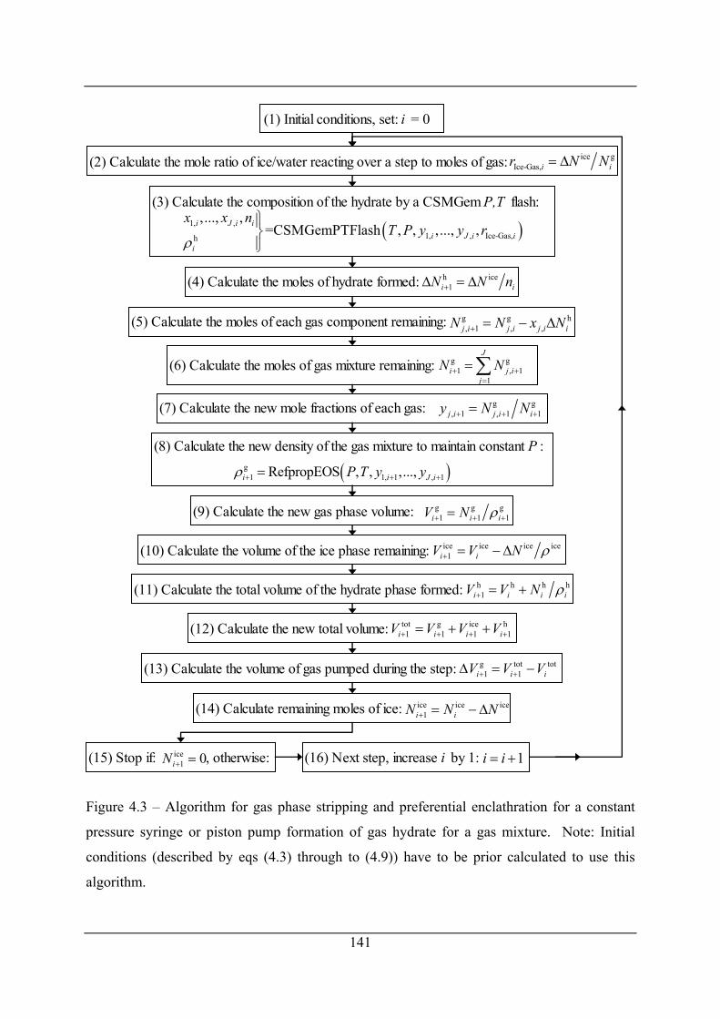
(1) Initial conditions, set: i = 0
g g1 , 1
1
J
i j ij
N N+ +=
=∑(6) Calculate the moles of gas mixture remaining:
g g, 1 , 1 1j i j i iy N N+ + +=(7) Calculate the new mole fractions of each gas:
(8) Calculate the new density of the gas mixture to maintain constant P :
( )g1 1, 1 , 1RefpropEOS , , ,...,i i J iP T y yρ + + +=
g g g1 1 1i i iV N ρ+ + +=(9) Calculate the new gas phase volume:
(10) Calculate the volume of the ice phase remaining: ice ice ice ice1i iV V N ρ+ = − Δ
(11) Calculate the total volume of the hydrate phase formed: h h h h1i i i iV V N ρ+ = +
(12) Calculate the new total volume: tot g ice h1 1 1 1i i i iV V V V+ + + += + +
(14) Calculate remaining moles of ice: ice ice ice1i iN N N+ = − Δ
(16) Next step, increase i by 1: 1i i= +(15) Stop if: , otherwise:ice1 0iN + =
(3) Calculate the composition of the hydrate by a CSMGem P,T flash:
( )1, ,1, , Ice-Gas,h
,..., ,=CSMGemPTFlash , , ,..., ,i J i i
i J i ii
x x nT P y y r
ρ
⎫⎪⎬⎪⎭
(2) Calculate the mole ratio of ice/water reacting over a step to moles of gas: ice gIce-Gas,i ir N N= Δ
(5) Calculate the moles of each gas component remaining: g g h, 1 , ,j i j i j i iN N x N+ = − Δ
(13) Calculate the volume of gas pumped during the step: g tot tot1 1i i iV V V+ +Δ = −
(4) Calculate the moles of hydrate formed: h ice1i iN N n+Δ = Δ
Figure 4.3 – Algorithm for gas phase stripping and preferential enclathration for a constant
pressure syringe or piston pump formation of gas hydrate for a gas mixture. Note: Initial
conditions (described by eqs (4.3) through to (4.9)) have to be prior calculated to use this
algorithm.
141
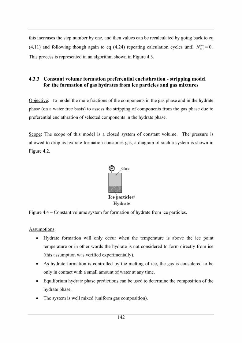
this increases the step number by one, and then values can be recalculated by going back to eq
(4.11) and following though again to eq (4.24) repeating calculation cycles until ice1 0iN + = .
This process is represented in an algorithm shown in Figure 4.3.
4.3.3 Constant volume formation preferential enclathration - stripping model for the formation of gas hydrates from ice particles and gas mixtures
Objective: To model the mole fractions of the components in the gas phase and in the hydrate
phase (on a water free basis) to assess the stripping of components from the gas phase due to
preferential enclathration of selected components in the hydrate phase.
Scope: The scope of this model is a closed system of constant volume. The pressure is
allowed to drop as hydrate formation consumes gas, a diagram of such a system is shown in
Figure 4.2.
Figure 4.4 – Constant volume system for formation of hydrate from ice particles.
Assumptions:
• Hydrate formation will only occur when the temperature is above the ice point
temperature or in other words the hydrate is not considered to form directly from ice
(this assumption was verified experimentally).
• As hydrate formation is controlled by the melting of ice, the gas is considered to be
only in contact with a small amount of water at any time.
• Equilibrium hydrate phase predictions can be used to determine the composition of the
hydrate phase.
• The system is well mixed (uniform gas composition).
142
• The temperature is uniform over entire system at any step.
• Vaporisation of water from the ice is considered negligible.
• The initial ratio of gas to water is great enough to ensure that complete conversion to
hydrate can occur.
• Initially values that are assumed to be known include:
o Mass of ice particles loaded into the cell.
o The total system volume.
o The pressure and temperature.
o The molar density of ice.
Equations: (a list of notation follows at the end of this section)
To model the constant volume pressure drop formation small steps were taken in the
conversion by taking small steps in pressure drop.
The initial part of the model is similar to the constant pressure model of the previous section
Firstly the initial amount of ice loaded into the pressure cell to form hydrate is considered.
The moles of ice initially loaded in to the cell (i = 0), , can be calculated by: ice0N
ice ice ice0 0N m M= , (4.25)
where is the mass of ice particles loaded in to the cell and Mice is the molar mass of ice
(water).
ice0m
The volume of the ice particles loaded in to the cell initially, , may be calculated from the
initial moles of ice, , and the molar density of ice, ρice:
ice0V
ice0N
ice ice ice0 0V N ρ= . (4.26)
The initial volume of the gas phase, , can then be calculated assuming the initial total
volume of the system, , is known:
g0V
tot0V
143
144
ce . (4.27) g tot i0 0 0V V V= −
The initial gas phase density, g0ρ , may be evaluated assuming knowledge of the composition
(mole fractions yj,i of component number j (of a total of J components) in the gas at
conversion step i), pressure and temperature. The Refprop equation of state (RefpropEOS)168
was used in calculations in this work:
( )g0 RefpropEOS , , ... JP T y yρ = 1,0 ,0
g g
0
. (4.28)
The initial number of moles of each gas in the mixture, , and the total moles of gas, ,
can then be calculated from:
g,0jN g
0N
, (4.29) g,0 ,0 0 0j jN y Vρ=
and
. (4.30) g g g g0 0 0 ,
1
J
jj
N V Nρ=
= =∑
Unlike the constant pressure model of the previous section, the pressure drop model takes a
step in pressure drop rather than conversion of ice to hydrate. The pressure step, ΔPstep, can
be set by taking a small fraction, X, of the pressure drop, ΔPdrop:
step dropP X PΔ = Δ (4.31)
Initially the mole ratio of water (ice) consumed to gas, , was set at: Ice-Gasr
Ice-Gas,0 0.01r = , (4.32)
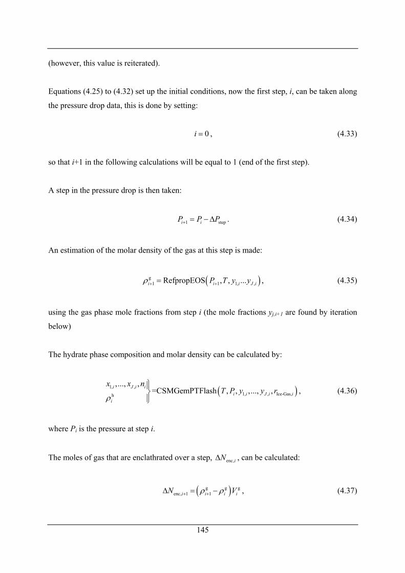
(however, this value is reiterated).
Equations (4.25) to (4.32) set up the initial conditions, now the first step, i, can be taken along
the pressure drop data, this is done by setting:
0i = , (4.33)
so that i+1 in the following calculations will be equal to 1 (end of the first step).
A step in the pressure drop is then taken:
1i iP P P+ step= −Δ . (4.34)
An estimation of the molar density of the gas at this step is made:
( )g1 1RefpropEOS , , ...i iP T y yρ + += 1, ,i J i
)
, (4.35)
using the gas phase mole fractions from step i (the mole fractions yj,i+1 are found by iteration
below)
The hydrate phase composition and molar density can be calculated by:
, (4.36) (1, ,1, , Ice-Gas,h
,..., ,=CSMGemPTFlash , , ,..., ,i J i i
i i J i ii
x x nT P y y r
ρ
⎫⎪⎬⎪⎭
where Pi is the pressure at step i.
The moles of gas that are enclathrated over a step, enc,iNΔ , can be calculated:
( )g genc, 1 1i i iN ρ ρ+ +Δ = − g
iV , (4.37)
145
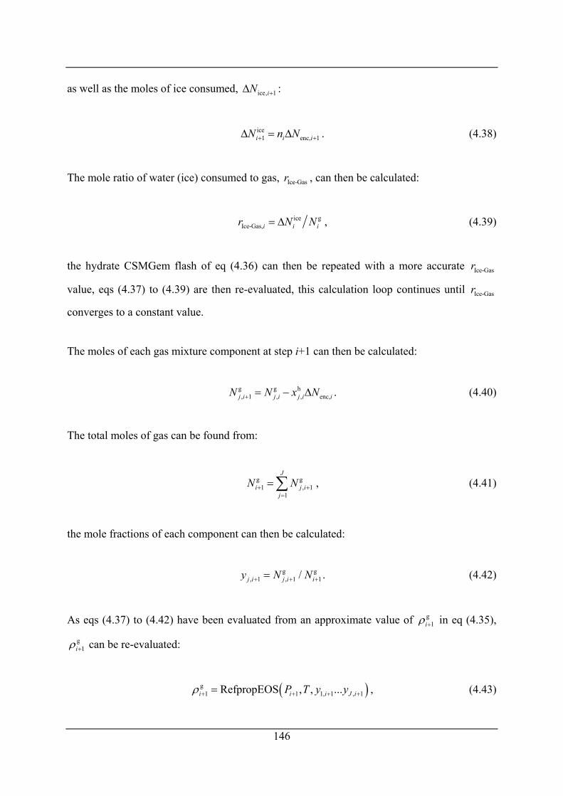
as well as the moles of ice consumed, ice, 1iN +Δ :
ice1 eni i iN n N c, 1+ +Δ = Δ . (4.38)
The mole ratio of water (ice) consumed to gas, , can then be calculated: Ice-Gasr
ice gIce-Gas,i ir N= Δ iN
g, 1j i
, (4.39)
the hydrate CSMGem flash of eq (4.36) can then be repeated with a more accurate
value, eqs
Ice-Gasr
Ice-Gasr(4.37) to (4.39) are then re-evaluated, this calculation loop continues until
converges to a constant value.
The moles of each gas mixture component at step i+1 can then be calculated:
. (4.40) g g h, 1 , , enc,j i j i j i iN N x N+ = − Δ
The total moles of gas can be found from:
g1
1
J
ij
N N+ +=
= ∑ , (4.41)
the mole fractions of each component can then be calculated:
g, 1 , 1 1/j i j i i
gy N N+ += + . (4.42)
As eqs (4.37) to (4.42) have been evaluated from an approximate value of g1iρ + in eq (4.35),
g1iρ + can be re-evaluated:
( )g1 1 1,RefpropEOS , , ...i i iP T y yρ + + += 1 , 1J i+ , (4.43)
146
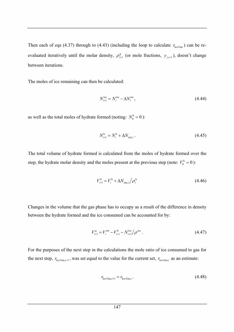
Then each of eqs (4.37) through to (4.43) (including the loop to calculate ) can be re-
evaluated iteratively until the molar density,
Ice-Gasr
g1iρ + (or mole fractions, ,j i 1y + ), doesn’t change
between iterations.
The moles of ice remaining can then be calculated:
, (4.44) ice ice ice1i iN N N+ = − Δ i
as well as the total moles of hydrate formed (noting: h0 0N = ):
. (4.45) h h1i iN N N+ = + Δ enc,i
The total volume of hydrate formed is calculated from the moles of hydrate formed over the
step, the hydrate molar density and the moles present at the previous step (note: ): h0 0V =
h h1 enc,i i iV V N h
iρ+ = + Δ (4.46)
Changes in the volume that the gas phase has to occupy as a result of the difference in density
between the hydrate formed and the ice consumed can be accounted for by:
g tot h ice i1 1 1i i i iV V V N ceρ+ + += − − . (4.47)
For the purposes of the next step in the calculations the mole ratio of ice consumed to gas for
the next step, , was set equal to the value for the current set, as an estimate: Ice-Gas, 1ir + Ice-Gas,ir
Ice-Gas, 1 Ice-Gas,ir r+ i= . (4.48)
147
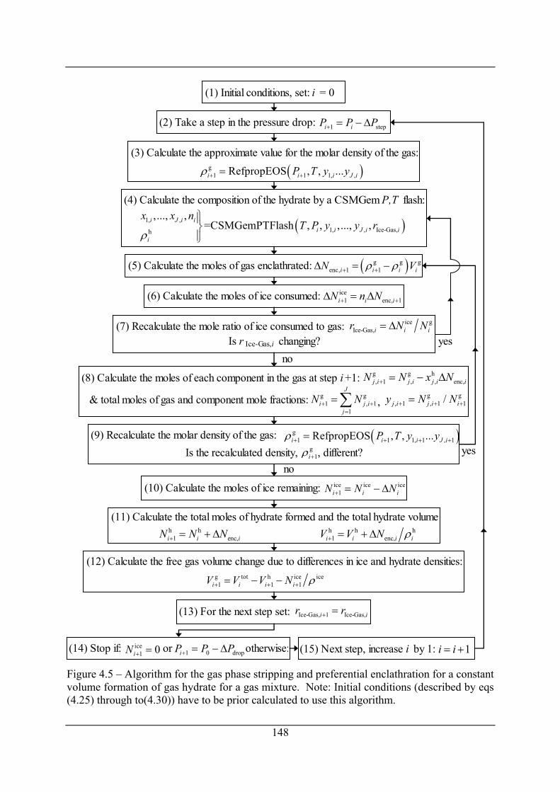
no
(1) Initial conditions, set: i = 0
(15) Next step, increase i by 1: 1i i= +
(2) Take a step in the pressure drop: 1 stepi iP P P+ = − Δ
(3) Calculate the approximate value for the molar density of the gas:
( )g1 1 1, ,RefpropEOS , , ...i i i J iP T y yρ + +=
yes
(11) Calculate the total moles of hydrate formed and the total hydrate volume h h h1 enc,i i i iV V N ρ+ = + Δh h
1 enc,i i iN N N+ = + Δ
(12) Calculate the free gas volume change due to differences in ice and hydrate densities:g tot h ice ice1 1 1i i i iV V V N ρ+ + += − −
(14) Stop if: or otherwise:1 0 dropiP P P+ = − Δice1 0iN + =
(4) Calculate the composition of the hydrate by a CSMGem P,T flash:
( )1, ,1, , Ice-Gas,h
,..., ,=CSMGemPTFlash , , ,..., ,i J i i
i i J i ii
x x nT P y y r
ρ
⎫⎪⎬⎪⎭
ice gIce-Gas,i i ir N N= Δ(7) Recalculate the mole ratio of ice consumed to gas:
Is r Ice-Gas,i changing? yesno
Ice-Gas, 1 Ice-Gas,i ir r+ =(13) For the next step set:
(10) Calculate the moles of ice remaining: ice ice ice1i i iN N N+ = − Δ
( )g1 1 1, 1 ,RefpropEOS , , ...i i i J iP T y yρ + + + +=(9) Recalculate the molar density of the gas: 1
Is the recalculated density, , different?g1iρ +
(8) Calculate the moles of each component in the gas at step i +1: g g h, 1 , , enc,j i j i j i iN N x N+ = − Δ
& total moles of gas and component mole fractions: g g1 , 1
1
J
i j ij
N N+ +=
=∑ g g, 1 , 1 1/j i j i iy N N+ + +=,
(6) Calculate the moles of ice consumed: ice1 enc, 1i i iN n N+ +Δ = Δ
(5) Calculate the moles of gas enclathrated: ( )g g genc, 1 1i i i iN Vρ ρ+ +Δ = −
Figure 4.5 – Algorithm for the gas phase stripping and preferential enclathration for a constant volume formation of gas hydrate for a gas mixture. Note: Initial conditions (described by eqs (4.25) through to(4.30)) have to be prior calculated to use this algorithm.
148
149
)If there is no ice left to convert ( ice1 0iN + = or alternatively the full amount of pressure drop
has been achieved calculations stop, otherwise a new step in the pressure
drop is taken, this is accomplished by taking a step in i:
( 1 0 dropiP P P+ = − Δ )
1i i= + . (4.49)
Calculations for the new step begin again at eq (4.34).
The calculations described in eqs (4.34) through to (4.49) are represented in the calculation
algorithm of Figure 4.5.
4.3.4 Notation for models Roman
f Small fraction in conversion of ice to hydrate (used in constant pressure model).
i Step counter.
M Molar mass.
m Mass.
N Number of moles of a component or phase.
n Hydrate number (ratio of moles of water to moles of gas in the hydrate phase).
P Pressure.
rice-gas Mole ratio of ice converted to hydrate over a step to total moles of gas mixture.
T Temperature
V Volume of phase.
X Small fraction of the total pressure drop (used in constant volume model).
x Hydrate phase mole fraction of a guest component on a water free basis.
y Gas phase mole fraction.
Greek
ΔN Changes in moles of a phase or component over a step.
ΔPdrop Total overall pressure drop (used in constant volume model).
ΔPstep Pressure drop step size (used in constant volume model).
150
ΔV Changes in the overall volume or volume of a phase over a step.
ρ Molar density.
Subscripts
0 An initial condition (step 0)
enc Indicates enclathrated over a step.
i Property at step i.
J Total number of components.
j Component number.
Superscripts
g Gas phase property.
h Hydrate phase property/
ice Ice phase property.
tot Total overall property.
4.4 Experimental work Experimental work in this chapter involves the preparation of a gas mixture of methane +
ethane for measurements of the gas phase composition during hydrate plug formation and the
final hydrate gas composition on a water free basis. During the hydrate plug formation
samples of the gas phase were taken and their compositions were measured by gas liquid
chromatography (GLC). The gas composition of the final hydrate was also measured by GLC.
4.4.1 Materials Materials were the same as where used at the University of Canterbury in Chapter 3, methane
was sourced from Linde Gas, U.K Ltd, with a purity of 99.975 %. Ethane was obtained from
BOC gases limited and had a purity of 99 %. These gases were used to prepare gas mixtures
without further purification. The water used to prepare ice for hydrate preparation was
distilled and deionised.
151
4.4.2 Gas mixture preparation A gas mixture of methane + ethane was prepared in situ in an ISCO 260D syringe pump by
the same method as described in section 3.3.2 of Chapter 3. The mole fraction of methane
desired for these experiments was 90 % and a mixture of this approximate mole fraction was
prepared from pure methane and a mixture of mole fractions 53 % methane + 46 % ethane.
The final pressure of this mixture was approximately 7.2 MPa for a syringe pump volume of
266 ml (pump full). Gas chromatography measurements (described in more detail below)
indicated mole fractions of (89.7 ± 0.3) % methane and (10.3 ± 0.3) % ethane. The technique
of taking a sample of gas is described in detail in the section 4.4.4.
4.4.3 Hydrate preparation The hydrate preparation method was essentially the same as the constant pressure formation
method described in section 3.3.3 of Chapter 3. Sieved ice particles were loaded in to a cell
and the cell was then filled with gas and maintained at a constant pressure using a syringe
pump during formation (note: all the experimental work of this chapter was completed at the
University of Canterbury). The system used was slightly different however and only utilised
the short/sample cell of Figure 3.16 described in section 3.3.3. A diagram of the system is
shown in Figure 4.6. The total system volume bound by valves (3, 13 and 21) and the
cylinder regulator was approximately 330 cm3, estimated from the volume of the lines, fittings
and cell (cell volume = 51 cm3). The liquid nitrogen cooled cell loaded with 19.3 g of ice
particles was place in a Polyscience model 9601 bath preset to 258 K. The cell was then
connected via a ¼ in (6.35 mm) Swagelok quick-connect fitting to valve 15. Platinum
resistance thermometers, PRT (Omega 100 Ω part number PR-11-2-100-1/16-12-E,
± 0.04 K), were then placed in the cell thermowell and in the bath (these were connected via a
multiplexer (a 16 channel analog Intech 2100-A16) to a computer for logging using a data
acquisition board (Advantech PCL-812G)). Air was removed from the cell by both
vacuuming and purging. Values (3, 8 and 21) were closed (note: some values marked closed
in Figure 4.6 remained closed during all these experiments and the ISCO pump was closed off
as it was full with the gas mixture), and vacuuming of the cell was initiated by the opening
valve 13 to the building vacuum system, this reduced the pressure to about 0.02 MPa. Valve
13 was then closed and the valve 8 (a High Pressure Equipment Co. 15-11-AF1 needle valve)
was carefully adjusted to bleed gas in to the system to a final pressure of between about (0.2
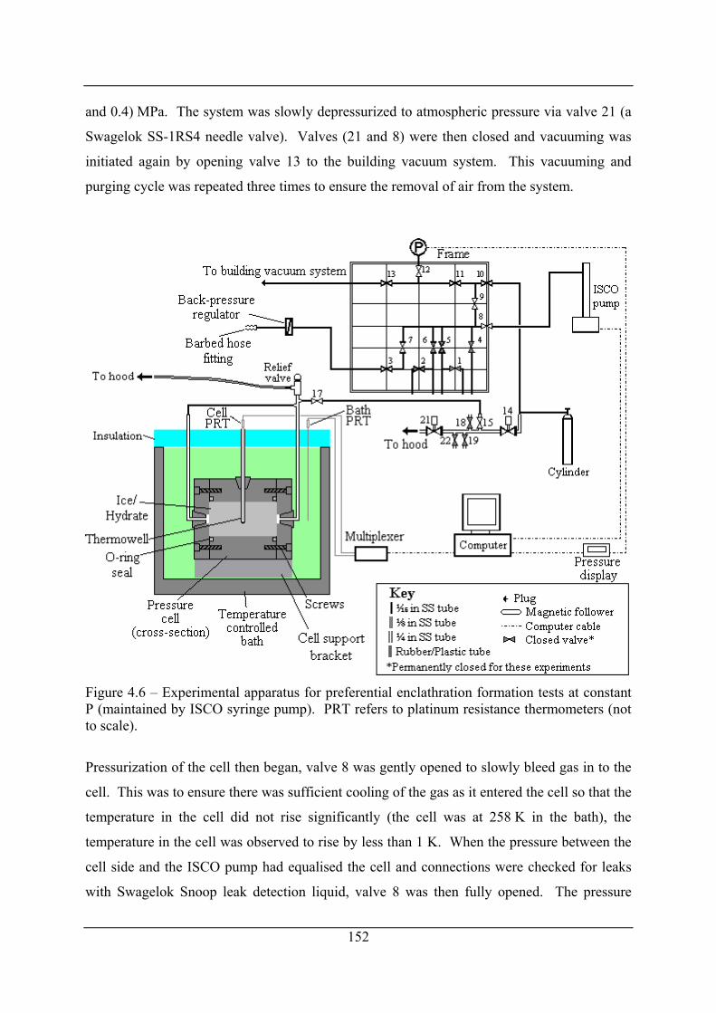
and 0.4) MPa. The system was slowly depressurized to atmospheric pressure via valve 21 (a
Swagelok SS-1RS4 needle valve). Valves (21 and 8) were then closed and vacuuming was
initiated again by opening valve 13 to the building vacuum system. This vacuuming and
purging cycle was repeated three times to ensure the removal of air from the system.
Figure 4.6 – Experimental apparatus for preferential enclathration formation tests at constant P (maintained by ISCO syringe pump). PRT refers to platinum resistance thermometers (not to scale).
Pressurization of the cell then began, valve 8 was gently opened to slowly bleed gas in to the
cell. This was to ensure there was sufficient cooling of the gas as it entered the cell so that the
temperature in the cell did not rise significantly (the cell was at 258 K in the bath), the
temperature in the cell was observed to rise by less than 1 K. When the pressure between the
cell side and the ISCO pump had equalised the cell and connections were checked for leaks
with Swagelok Snoop leak detection liquid, valve 8 was then fully opened. The pressure
152
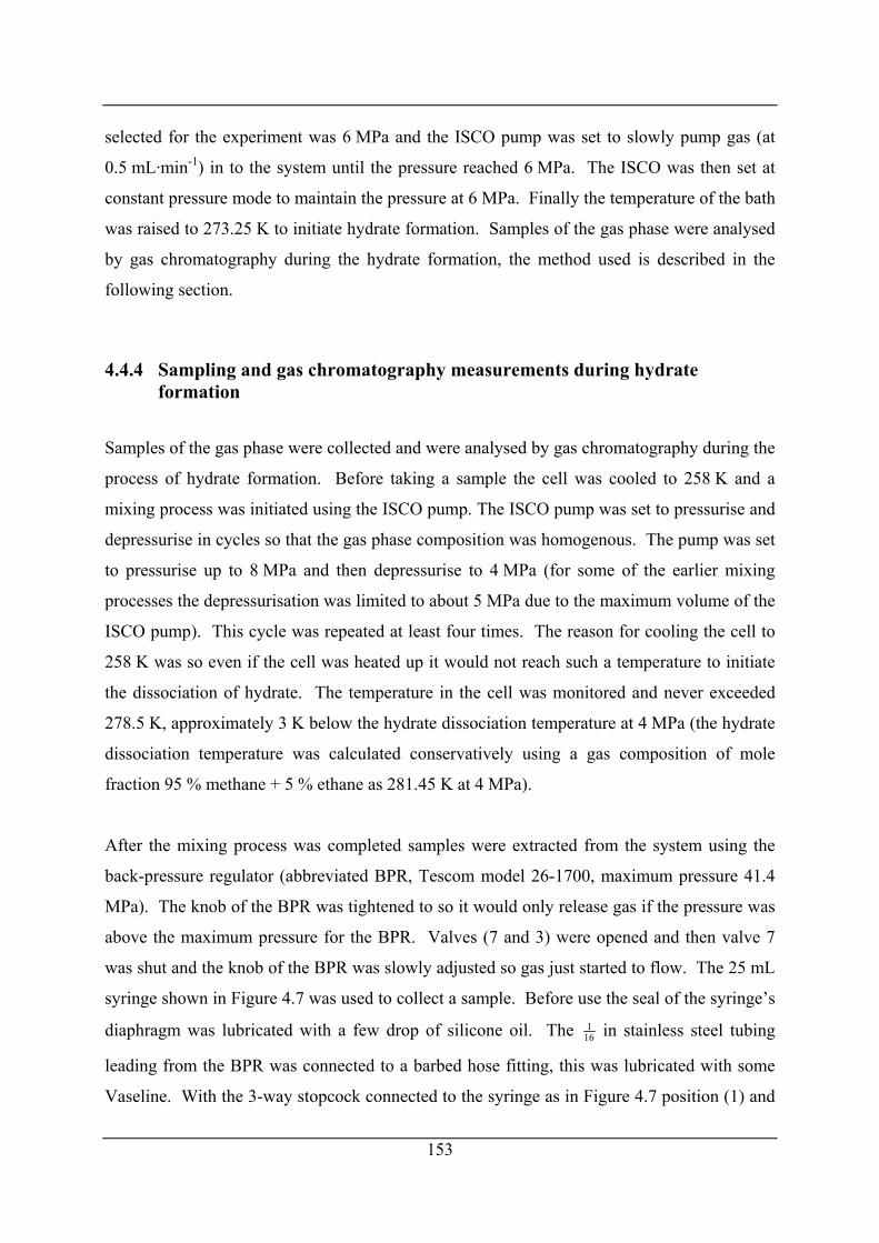
selected for the experiment was 6 MPa and the ISCO pump was set to slowly pump gas (at
0.5 mL·min-1) in to the system until the pressure reached 6 MPa. The ISCO was then set at
constant pressure mode to maintain the pressure at 6 MPa. Finally the temperature of the bath
was raised to 273.25 K to initiate hydrate formation. Samples of the gas phase were analysed
by gas chromatography during the hydrate formation, the method used is described in the
following section.
4.4.4 Sampling and gas chromatography measurements during hydrate formation
Samples of the gas phase were collected and were analysed by gas chromatography during the
process of hydrate formation. Before taking a sample the cell was cooled to 258 K and a
mixing process was initiated using the ISCO pump. The ISCO pump was set to pressurise and
depressurise in cycles so that the gas phase composition was homogenous. The pump was set
to pressurise up to 8 MPa and then depressurise to 4 MPa (for some of the earlier mixing
processes the depressurisation was limited to about 5 MPa due to the maximum volume of the
ISCO pump). This cycle was repeated at least four times. The reason for cooling the cell to
258 K was so even if the cell was heated up it would not reach such a temperature to initiate
the dissociation of hydrate. The temperature in the cell was monitored and never exceeded
278.5 K, approximately 3 K below the hydrate dissociation temperature at 4 MPa (the hydrate
dissociation temperature was calculated conservatively using a gas composition of mole
fraction 95 % methane + 5 % ethane as 281.45 K at 4 MPa).
After the mixing process was completed samples were extracted from the system using the
back-pressure regulator (abbreviated BPR, Tescom model 26-1700, maximum pressure 41.4
MPa). The knob of the BPR was tightened to so it would only release gas if the pressure was
above the maximum pressure for the BPR. Valves (7 and 3) were opened and then valve 7
was shut and the knob of the BPR was slowly adjusted so gas just started to flow. The 25 mL
syringe shown in Figure 4.7 was used to collect a sample. Before use the seal of the syringe’s
diaphragm was lubricated with a few drop of silicone oil. The 116 in stainless steel tubing
leading from the BPR was connected to a barbed hose fitting, this was lubricated with some
Vaseline. With the 3-way stopcock connected to the syringe as in Figure 4.7 position (1) and
153
the plunger was pushed fully in to flush out most of the air, and the rubber tubing was then
slipped over the barbed hose fitting and the plunger was forced back slowly with the flow of
gas from the BPR. When the plunger was near full the stopcock was changed to position (3)
and the rubber tubing was quickly removed from the barbed hose fitting. The syringe was
then flushed out again by holding the rubber tubing between the finger tips to generate a flow
restriction (to prevent inward flow of air) the stopcock was changed to position (1) and the
plunger was pressed down steadily. The stopcock was changed to position (3) when the
plunger was close to fully pushed-in. A fresh sample of gas was then collected by the method
just described. This flushing procedure was repeated at least three times. The BPR knob was
then slowly turned to lower pressure until the gas flow was stopped. This was done to bleed
the gas from the line leading to the BPR so not to cause contamination for the next
measurement.
gas sample25 ml syringe plunger
(1) 3-way stopcockin 3-way open postion(for gas sample filling)
rubbertubeSeptum
(2) 3-way stopcock open to25 ml syringe and septum (for 1 ml syringe samples)
(3) 3-way stopcock closed in all 3-ways
(between taking samples)
Alternative3-way stopcock
positions
diaphragm seal
Figure 4.7 – Syringe used to gas samples showing alternative positions of the 3-way stopcock.
The 25 mL syringe was then used to provide samples of approximately 0.3 mL for gas
chromatography. These samples were taken from the 25 mL syringe via the 3-way stopcock
septum (the stopcock was position (2) of Figure 4.7). The syringe used to extract the samples
was a Valco Instruments series A-2 1 mL syringe with a push button valve. The 1 mL syringe
was flushed approximately ten times with the gas from the 25 mL syringe, the push button
valve was then closed and the needle was removed from the septum.
154
The sample was then injected into the gas chromatograph. The chromatograph used was a
Shimadzu GC-R1A with a RPR-G1 GC-processor and chart recorder. A 1.83 m (6 ft),
6.35 mm (¼ in) O.D Porapak Q packed column was utilized with a TCD detector. The
injection and detection temperatures were 423 K and the column temperature was 318 K. The
flow rate or helium was set to 25 mL min-1. Experimentally it was impossible to remove all
the air from the samples and a small amount was always present, the oxygen and nitrogen
peaks were indistinguishable and formed a single air peak. If there was significant air
contamination a fresh sample was collected using the 25 mL syringe. Contamination was
considered to be too large when the resolution of the air and the methane peak was below 1.5.
Typical elution times for air, methane and ethane were about 1.2 min, 1.75 min and 8.9 min
respectively. For each 25 mL syringe of gas 6 to 10 injections were completed so that errors
in the compositions measured could be estimated.
4.4.5 Hydrate phase measurements and structural identification When the consumption of gas, indicated by no flow from the ISCO pump (set to pump at
constant pressure), had ended the hydrate formation was considered ended and valve (15 and
17) of Figure 4.6 were closed. An 116 in (6.35 mm) Swagelok fitting at valve 15 was then
carefully untightened and the gas from this line was bled in to the room (this was only a small
volume, less than 15 mL at STP, as the tube diameter was 116 in). The cell was then
disconnected from the system and placed in a bath of liquid nitrogen in the hood. The
temperature continued to be monitored by the cell PRT (using an extension cable from the
multiplexer) and when the temperature inside the cell had dropped to below 180 K valve 17
was opened carefully to depressurise the cell to the hood (under these conditions the hydrate
should be stable at atmospheric pressure). Once the cell was completely depressurized the
cell was carefully tipped on to one of ends so that the screws and lid of the other end could be
removed. The hydrate inside the cell was then quickly scrapped out with a liquid nitrogen
cooled spoon and was placed into a Dewar flask also containing liquid nitrogen.
The water free gas composition of the hydrate was measured by dissociating samples of the
hydrate within the 25 mL syringe. A lump or several lumps (of perhaps several cm3) of
hydrate from the liquid nitrogen Dewar flask were quickly removed and placed in the 25 mL
155
156
syringe that had its plunger removed. The plunger was then reinserted with the stopcock of
Figure 4.7 in position (1) and the plunger pushed down as far as possible (even if it meant
breaking the lumps of hydrate apart). The rubber hose was held between fingertips initially
due to an initial large release of gas assumed to be the vaporisation of the liquid nitrogen.
When the hydrate was observed to bubble and fizz the stopcock was changed to position (3)
and the syringe plunger was allowed to be pushed back by the pressure of the gas from the
dissociating hydrate in the syringe. When the volume of gas was close to 25 mL the stopcock
was changed back to position (1) and the gas was expelled by pressing the plunger with
fingertip compressing the rubber hose to create a flow restriction. After the gas had been
expelled the stopcock was switched back to position (3) and the syringe once again started to
be filled with the gas from the dissociating hydrate. This process of expelling the gas when
the plunger reached a volume near 25 mL was repeated until all the hydrate had dissociated.
However enough gas was left in the syringe to take samples for gas chromatography. The
chromatographic method used for these samples was the same as previously described above,
although special care was taken due to water in the 25 mL syringe. The syringe was held
upside down so that the water drained to the plunger end away from the stopcock and septum
where the samples for gas chromatography were removed.
4.4.6 Modelling the experiments The model presented in section 4.3.2 of this chapter presents somewhat of an ideal model as
the temperature of the entire system was assumed to be uniform. This however was not the
case experimentally. In the system shown in Figure 4.6 the cell was in a temperature
controlled bath and the ISCO syringe pump was at room temperature. The property affected
by this difference in temperature was the molar density of the gas in the system. Instead of
assuming one temperature for the whole system the density was calculated at the average
room temperature during experiments and the cell temperature and the density was volume
averaged for the approximate volumes of gas at each temperature. Equations (4.7) and (4.17)
were replaced by:
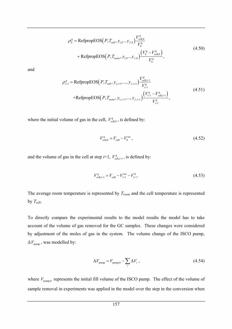
( )
( ) ( )
gcell,0g
0 cell 1,0 ,0 g0
g g0 cell,0
room 1,0 ,0 g0
RefpropEOS , , ...
RefpropEOS , , ... ,
J
J
VP T y y
V
V VP T y y
V
ρ =
−+
(4.50)
and
( )
( ) ( )
gcell,i+1g
1 cell 1, 1 , 1 gi+1
g gi+1 cell,i+1
room 1, 1 , 1 gi+1
RefpropEOS , , ,...,
+RefpropEOS , , ,..., ,
i i J i
i J i
VP T y y
V
V VP T y y
V
ρ + + +
+ +
=
− (4.51)
where the initial volume of gas in the cell, , is defined by: gcell,0V
, (4.52) gcell,0 cell 0V V V= − ice
h
and the volume of gas in the cell at step i+1, , is defined by: gcell,i+1V
. (4.53) g icecell,i+1 cell i+1 i+1V V V V= − −
The average room temperature is represented by Troom and the cell temperature is represented
by Tcell.
To directly compare the experimental results to the model results the model has to take
account of the volume of gas removed for the GC samples. These changes were considered
by adjustment of the moles of gas in the system. The volume change of the ISCO pump,
Δ pumpV , was modelled by:
pump pump,0 ii
V VΔ = − ΔV∑ , (4.54)
where pump,0V represents the initial fill volume of the ISCO pump. The effect of the volume of
sample removal in experiments was applied in the model over the step in the conversion when
157
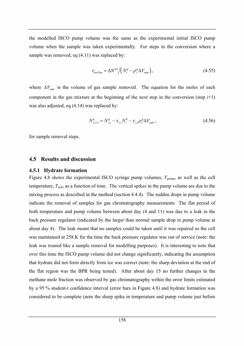
the modelled ISCO pump volume was the same as the experimental initial ISCO pump
volume when the sample was taken experimentally. For steps in the conversion where a
sample was removed, eq (4.11) was replaced by:
( )ice g gIce-Gas sami ir N N Vρ= Δ − Δ , (4.55)
where is the volume of gas sample removed. The equation for the moles of each
component in the gas mixture at the beginning of the next step in the conversion (step i+1)
was also adjusted, eq
samVΔ
(4.14) was replaced by:
, (4.56) g g h g, 1 , , , samj i j i j i i j i iN N x N y Vρ+ = − − Δ
for sample removal steps.
4.5 Results and discussion
4.5.1 Hydrate formation Figure 4.8 shows the experimental ISCO syringe pump volumes, Vpump, as well as the cell
temperature, Tcell, as a function of time. The vertical spikes in the pump volume are due to the
mixing process as described in the method (section 4.4.4). The sudden drops in pump volume
indicate the removal of samples for gas chromatography measurements The flat period of
both temperature and pump volume between about day (4 and 11) was due to a leak in the
back pressure regulator (indicated by the larger than normal sample drop in pump volume at
about day 4). The leak meant that no samples could be taken until it was repaired so the cell
was maintained at 258 K for the time the back pressure regulator was out of service (note: the
leak was treated like a sample removal for modelling purposes). It is interesting to note that
over this time the ISCO pump volume did not change significantly, indicating the assumption
that hydrate did not form directly from ice was correct (note: the sharp deviation at the end of
the flat region was the BPR being tested). After about day 15 no further changes in the
methane mole fraction was observed by gas chromatography within the error limits estimated
by a 95 % student-t confidence interval (error bars in Figure 4.8) and hydrate formation was
considered to be complete (note the sharp spike in temperature and pump volume just before
158
day 20 occurred after the cell had been disconnected and chilled in liquid nitrogen to extract
hydrate samples).
0
50
100
150
200
250
300
0 5 10 15 20t /days
Vpu
mp/m
L
243.15
253.15
263.15
273.15
283.15
293.15
303.15
Tce
ll/K
Pump VolumeCell temperature
Figure 4.8 – Volume of the ISCO syringe pump and temperature of the cell as a function of time.
The desired pressure for the formation of the hydrate was 6 MPa. The average pressure over
the time of the formation was 6.03 MPa, this value was used in the model. The room
temperature (used in calculations of the overall gas density) was an averaged value of 294.7 K
over the time of the formation, the maximum variation from this temperature was ± 2.8 K. A
step size in the conversion of ice to hydrate was set by selecting an f value for eq (4.4) of 0.02.
4.5.2 Gas chromatography results and comparison to model Figure 4.9 shows mole fraction of methane in the gas phase as a function of the volume
pumped from the ISCO syringe pump both from experimental gas chromatography
measurements and the constant pressure model. The flat regions of constant composition
represent the points when samples were removed, and the change in the pump volume with no
159
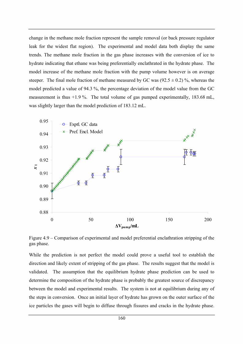
change in the methane mole fraction represent the sample removal (or back pressure regulator
leak for the widest flat region). The experimental and model data both display the same
trends. The methane mole fraction in the gas phase increases with the conversion of ice to
hydrate indicating that ethane was being preferentially enclathrated in the hydrate phase. The
model increase of the methane mole fraction with the pump volume however is on average
steeper. The final mole fraction of methane measured by GC was (92.5 ± 0.2) %, whereas the
model predicted a value of 94.3 %, the percentage deviation of the model value from the GC
measurement is thus +1.9 %. The total volume of gas pumped experimentally, 183.68 mL,
was slightly larger than the model prediction of 183.12 mL.
0.88
0.89
0.90
0.91
0.92
0.93
0.94
0.95
0 50 100 150 200ΔVpump/mL
x1
Exptl. GC dataPref. Encl. Model
Figure 4.9 – Comparison of experimental and model preferential enclathration stripping of the gas phase.
While the prediction is not perfect the model could prove a useful tool to establish the
direction and likely extent of stripping of the gas phase. The results suggest that the model is
validated. The assumption that the equilibrium hydrate phase prediction can be used to
determine the composition of the hydrate phase is probably the greatest source of discrepancy
between the model and experimental results. The system is not at equilibrium during any of
the steps in conversion. Once an initial layer of hydrate has grown on the outer surface of the
ice particles the gases will begin to diffuse through fissures and cracks in the hydrate phase.
160
161
Diffusive separation of the gases is not likely to occur by mechanisms such as Knudsen
diffusion however due to the elevated pressure reducing the mean free paths of the molecules.
Once the hydrate has coated all the surfaces including the surfaces insides the fissures and
cracks further conversion to hydrate occurs by diffusion through a layer of hydrate. Due to
the size of methane it is believed that it will diffuse through the hydrate layer more easily than
ethane. Ethane may have to be orientated longitudinally to pass through the hydrate layer. It
might be expected for this reason that the hydrate phase would form with a higher proportion
of methane than would be predicted by equilibrium thermodynamics. This could explain the
discrepancy between the model predictions and experimental measurements observed in
Figure 4.9.
The GC measured water free mole fraction of methane in the hydrate phase was (78.5 ±
0.7) % compared to a prediction of the model of 73.3 %. The difference of 5.2 % is larger in
comparison to the difference for the final gas phase methane mole fraction. A possible cause
was that the sampling method for the GC measurement was for a sample that was non-
representative of the overall hydrate. In retrospect it may have been better to powder the
entire hydrate sample and mix it (under the presence of liquid nitrogen in a mortar and pestle).
On the other hand the model predicts greater stripping of ethane from the gas phase than the
GC experimental results indicate, this should and does result in a lower methane mole fraction
in the hydrate.
The sample of hydrate tested by X-ray diffraction indexed to a sII hydrate as expected. The
gas phase mole fractions did not change enough to result in the formation of sI hydrate. If the
amount of ice loaded initially into the cell was larger, or the amount of initial gas was less,
then this might have been a possibility as both the experimental results and the model
predicted that the gas phase methane mole fraction increased with the conversion of ice to
hydrate, becoming closer to the structural transition value of approximately 99.3 % (as
measured by Subramanian et al.71).
4.5.3 Constant volume model The constant volume method was used to estimate the degree of stripping from the gas phase
due to preferential enclathration for methane + ethane mixtures in Chapter 3. As the method
162
used in the constant volume method is similar to the constant pressure method it is possible to
assume that this method is validated. Like the constant pressure model it should be noted that
the constant volume model would not be expected to make perfect predictions (if
implemented similarly to the prediction presented in Figure 4.9).
Figure 3.19 of Chapter 3 shows the predicted mole fraction of methane in the gas phase, x1, as
a function of the pressure (dashed curve) for a constant volume hydrate formation at 273.25 K
from a mixture with a methane mole fraction of 98.8 % and an ethane mole fraction of 1.2 %
initially at a pressure of 8.2 MPa. The curve indicates not much pressure drop would be
needed under the conditions detailed to result in stripping of the gas phase from a sII forming
region to a sI forming region.
Figure 3.24 of Chapter 3 shows the predicted mole fraction of methane in the gas phase, x1, as
a function of pressure (pressure/compositional tracking curve) for a constant volume hydrate
formation at 273.25 K from a mixture with a methane mole fraction of 65.4 % and an ethane
mole fraction of 34.6 % initially at a pressure of about 14.1 MPa. The gas composition used
in this hydrate formation is close to the composition at which hydrate phase water free mole
fractions of each component are predicted to be the same as the gas phase (see Figure 3.18).
As a result of this the predicted stripping of the gas phase by the model was low (ethane
fraction increased slightly in the gas phase). Crossing the sII to sII phase boundary due to too
much pressure drop rather than gas phase component stripping was more of a concern for this
formation. The cell was repressurized during the formation to prevent this from happening.
No direct measurements to determine the accuracy of the constant volume model were
performed and the method has been assumed valid based on the results of the constant
pressure method success. An experimental study further investigated the accuracy of the
model.
4.5.4 Stepwise models for hydrate formation The models for stepwise hydrate formation could potentially be adapted further. The
temperature for example could be allowed to vary with each step, this would allow
calculations of gas phase stripping and preferential enclathration for a gas mixture to be
performed for a constant volume system that is heated and/or cooled under hydrate forming
conditions. The pressure may not drop for all steps if such adaptations were made however so
they would have to also be fed in to the model at each step as well. The hydrate formation
method described by Stern et al.126 for the formation of hydrate from pure methane involved
significant heating and cooling, the model could be applied to similar hydrate formations with
gas mixtures.
The constant volume, (written before the constant pressure model) could potentially be
rewritten in terms of conversion of a small fraction of ice to make it more like the constant
pressure model. The current model is very slow to implement due to the two internal loops
to, one, calculate the mole ratio of ice consumed per step to gas (rIce-Gas) and, two, calculate
the molar density of the gas at the next step ( g1iρ + ) (the fact that these loops interact certainly
doesn’t help either).
The models produced in this work could potentially be applied to situations other than
laboratory hydrate plug formation. They may be useful in the modelling of separation
processes utilising gas hydrates. The constant volume model could be applied to a batch
separation process of a gas mixture. Hydrate could be formed from the mixture from an
initial pressurisation in a closed vessel. The system could be cooled after sufficient
conversion to low temperature so that the hydrate would be stable following removal of most
of the gas phase. The gas phase could then be mostly removed by depressurising the vessel
and the hydrate could be dissociated. Similarly the constant pressure syringe pump model
could be used if the pressure was maintained constant in such a vessel by a syringe or piston
pump (without flow of fresh gas in to the system).
Another potentially useful model would be one derived for an open-system at constant
pressure where the gas pressure is regulated in the system by flow from a cylinder or other
supply. This model was not generated in this work but could be by using similar assumptions
and equations. Using this method with two different gas mixtures it may be possible to
prevent changes in the gas phase composition during hydrate formation (see next subsection).
163
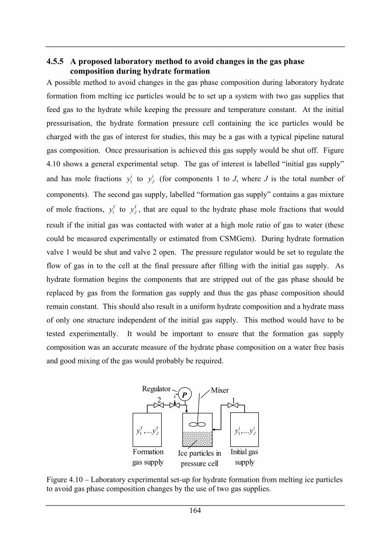
4.5.5 A proposed laboratory method to avoid changes in the gas phase composition during hydrate formation
A possible method to avoid changes in the gas phase composition during laboratory hydrate
formation from melting ice particles would be to set up a system with two gas supplies that
feed gas to the hydrate while keeping the pressure and temperature constant. At the initial
pressurisation, the hydrate formation pressure cell containing the ice particles would be
charged with the gas of interest for studies, this may be a gas with a typical pipeline natural
gas composition. Once pressurisation is achieved this gas supply would be shut off. Figure
4.10 shows a general experimental setup. The gas of interest is labelled “initial gas supply”
and has mole fractions to i1y i
Jy (for components 1 to J, where J is the total number of
components). The second gas supply, labelled “formation gas supply” contains a gas mixture
of mole fractions, f1y to f
Jy , that are equal to the hydrate phase mole fractions that would
result if the initial gas was contacted with water at a high mole ratio of gas to water (these
could be measured experimentally or estimated from CSMGem). During hydrate formation
valve 1 would be shut and valve 2 open. The pressure regulator would be set to regulate the
flow of gas in to the cell at the final pressure after filling with the initial gas supply. As
hydrate formation begins the components that are stripped out of the gas phase should be
replaced by gas from the formation gas supply and thus the gas phase composition should
remain constant. This should also result in a uniform hydrate composition and a hydrate mass
of only one structure independent of the initial gas supply. This method would have to be
tested experimentally. It would be important to ensure that the formation gas supply
composition was an accurate measure of the hydrate phase composition on a water free basis
and good mixing of the gas would probably be required.
Mixer1
Ice particles inpressure cell
Initial gassupply
RegulatorP2
Formationgas supply
f f1 ,... Jy y i i
1 ,... Jy y
Figure 4.10 – Laboratory experimental set-up for hydrate formation from melting ice particles to avoid gas phase composition changes by the use of two gas supplies.
164
165
Chapter 5 TETRAISOPENTYLAMMONIUM FLUORIDE + METHANE SEMI-CLATHRATE HYDRATE PHASE MEASUREMENTS
5.1 Introduction A general introduction to semi-clathrate hydrates (SCH) is presented in Chapter 1 of this
work, including elements of their cage structures and stoichiometry. In brief, some host
hydrate water lattice sites in a SCH are replaced by a peralkylonium cation central atom (such
as the N atom of tetraisopentylammonium ion) and the anion. Typically SCH of
peralkylonium salts with butyl or isopentyl alkyl chains are most stable, some have melting
points as high as the mid 30 °Cs. As the water lattice is broken Davidson11 suggested the
term “semi-clathrate hydrate” rather than “clathrate hydrate”. Structural studies reveal that
these SCH contain vacant cages (see Davidson,11 Dyadin and Udachin3 and Jeffrey4 for
general reviews of SCH structures). At the end of the review of SCH in Chapter 1, gas
storage in SCH was discussed with particular emphasis on optimising the gas storage
capability, determined by the relative numbers of vacant cages per unit mass or volume of the
SCH. The temperature stability of the SCH was also considered. An advantageous property
for a SCH for gas storage would be if no refrigeration was required to keep the SCH stable
and only slight heating or depressurisation was required to release the stored gas. From these
consideration tetraisopentylammonium fluoride with the structural hydration number of 38
(TIPAF·38H2O) appeared to be a good candidate.
This chapter focuses on the stability of TIPAF + water + methane at pressures higher than
atmospheric and hence temperatures higher than the atmospheric pressure melting point. The
measurements were performed for one concentration or hydration number of TIPAF and
water. The TIPAF to water mole ratio was fixed by crystallizing the hydrate with structural
hydration number of 38. This hydration number was measured by Karl Fischer titration to be
38.3. The P,T equilibria measured were semi-clathrate hydrate + aqueous solution + vapour
(SCH + Aq + V) points, in the temperature range from about (309 to 320) K.
166
5.2 Enclathration of gases by semi-clathrate hydrates – literature review As noted in the introduction the first observation of the ability of a SCH to enclathrate gas
molecules was that of McMullan et al.61 when they noted the release of gas as
tetrabutylammonium fluoride crystals melted. They determined that this gas was air, by gas
chromatography. Jeffrey4, Davidson11 and Shimada et al.63 made similar observations.
The first specific investigation of the enclathration of gas molecules in a SCH was by Stupin
and Stravitnaya.65,66 They measured the adsorption of sulfur dioxide by the SCHs of
tetraisopentylammonium and tetrabutylammonium phthalates as well as tetrabutylammonium
bromide and acetate (TBAB and TBAAc). For their study with TBAB and TBAAc the
stoichiometry of the SCHs were TBAB·24H2O and TBAAc·31.4H2O respectively.5 The
sulfur dioxide was absorbed at low pressure (8 to 30) kPa and temperatures between (253 and
277) K, below the melting point of the SCH. The gas was adsorbed in to the SCHs in a
pressure cell containing spherical PTFE beads that was mechanically shaken in an isothermal
low temperature bath (Stupin and Stravitnaya note that this method was the same as used by
Barrer and Edge152 for the formation gas hydrates from ice and argon, krypton and xenon).
The pressure at which adsorption occurred was kept constant by raising the level of mercury
in a gas burette to reduce the volume of the system to compensate for the adsorbed gas. The
volume of gas adsorbed could be calculated from the volume reduction (mercury level). The
pressure was then slightly lowered in the pressure cell which resulted in the slow desorption
over (2 to 3) h of gas from the SCH. The pressure was kept constant by lowering the level of
mercury in the gas burette until desorption ended. The volume of gas released could then be
calculated. The pressure reduction step was repeated several further times. A full set of
measurements were then repeated at different bath temperatures. These measurements
allowed the calculation of Langmuir isotherm adsorption constants. Interestingly Stupin and
Stravitnaya suggest that methane or argon could not be adsorbed in to the TBAB·24H2O SCH
“even at 195 K and 80 kPa”.5 More recent literature, outlined in paragraphs below, indicate
methane can be enclathrated in at least some structures of TBAB SCH.
From observations that SCH formed from an aqueous solution of TBAB under atmospheric
conditions released bubbles of gas, Shimada et al.63 decided to investigate whether other gas
molecules could be enclathrated. Mixtures of methane + ethane, methane + propane and pure
167
propane were investigated. In a pressure vessel the gas at a pressure of 1.0 MPa was sparged
through a 10 % mass fraction solution of TBAB in water while cooling the solution from (20
to 1) °C. Crystals of SCH that formed were removed from the solution and heated in a small
vessel, the released gas was then analysed by gas chromatography. Firstly the mixtures of
methane + propane and methane + ethane where tested and it was shown that the gas released
upon dissociation of the SCH was mainly methane. Experiments were then conducted with
pure propane, however no gas bubbles were observed as the SCH dissociated. This lead
Shimada et al. to believe that ethane and propane were only present in small amounts for the
methane mixture experiments because the crystals that were dissociated where wetted with
TBAB solution in which these components were dissolved. The structures of TBAB SCH
were then investigated by X-ray crystallography and it was determined that the only vacant
cages present were dodecahedral 512 cages. One structure had already been presented in
Davidson11 the other structure found was unknown, this structure was later investigated by
X-ray crystallography by Shimada et al.62 and was found to be TBAB·38H2O. The lack of
vacant cages larger than the 512 cage explained why propane was not enclathrated. Shimada et
al. then suggest that TBAB SCH would provide a suitable method of separation of methane
from ethane and propane. The separation of gases was further investigated in the paper by
Kamata et al.64 Five binary gas mixtures of methane + ethane, methane + propane, methane +
hydrogen sulfide, methane + nitrogen and carbon dioxide + hydrogen sulfide were
investigated (all at several different compositions) again using a 10 % mass fraction solution
of TBAB. The gases were sparged through a prior evacuated pressure vessel at 1.0 MPa that
was cooled from (20 to 0) °C. Samples of SCH were removed and wiped with hygroscopic
paper and then placed in a 60 mL pressure vessel at -10 °C that was then evacuated. The
pressure vessel was then heated to 25 °C to dissociate the SCH and the gas compositions were
measured by gas chromatography. The TBAB SCH formed with the methane + ethane and
methane + propane mixtures only enclathrated methane. For the methane + hydrogen sulfide
mixtures over 95 % of the hydrogen sulfide was removed at all initial compositions (the
hydrogen sulfide composition ranged from a mole fraction of (0.02 to 0.61) % in the initial
vapour phase) This was explained by the fact that the solubility of H2S is two orders of
magnitude greater than CH4 in water. The SCH formed from methane + nitrogen gas
contained both components but the methane content of the SCH was between (10 and 30) %
higher than the initial gas composition that was varied between a mole fraction of (10 and 80)
168
%. For the CO2 + H2S mixture it was found that the SCH enclathrates about 90 % of the
initial vapour phase H2S and it was concluded that CO2 could probably not enter the vacant
512 cage of the TBAB SCH as it is too large (note: more measurements with TBAB solutions
and “biogas” mixtures methane and carbon dioxide containing less than 1 % mole fraction
H2S were published several years later by Kamata et al.169 with similar results). Overall it
was suggested that the size limits of molecules that can be enclathrated in the 512 cages of the
TBAB SCH are the same as the limits for the 512 cages of gas hydrates.
The first measurements on the three phase SCH + aqueous solution + vapour (SCH + Aq + V)
P,T equilibria system were those of Hashimoto et al.46 for a mole fraction of 3.6 % TBAB in
solution + hydrogen. This concentration of TBAB was selected to correspond to a 40 % mass
fraction solution, that had been shown to be near the T,x phase diagram temperature
maximum for TBAB + water by Shimada et al.63 The solution of TBAB was introduced to an
evacuated high pressure cell and pressurised with hydrogen. Agitation in the cell was
provided using a mixing bar, driven by an exterior permanent magnetic ring. The high
pressure cell contained a window from which the three phase condition could be observed
visually. The three phase condition was established at constant temperature by adjusting the
pressure of hydrogen. The window of the pressure cell also allowed in situ Raman
measurements of all three phases present. Raman data from the SCH phase confirmed the
occupation of the 512 cages by hydrogen. The P,T three phase equilibria measurements were
made in the temperature range from (285.4 to 287.3) K which resulted in equilibrium
pressures between (0.13 and 13.6) MPa. In a recent paper Hashimoto et al.46 repeated a
similar set of measurements at TBAB mole fractions of 0.6 %, 2.0 % and 7.0 %, these
measurements as well as those from the original paper are shown in Figure 5.1. From
measurements on the T,x phase equilibrium of TBAB + water at atmospheric conditions it
was assumed that the solution at the mole fraction of 0.6 % would form a different structure
of SCH to that of the higher concentrations (and the 3.6 % mole fraction solution from the
original paper). Raman measurements were again used to confirm that hydrogen had entered
the cages of all SCH formed. The P,T phase measurements revealed similarly shaped three
phase curves for each concentration of solution, each curve coincided with their respective
points on the T,x phase equilibrium of TBAB + water at atmospheric pressure. In other words
the TBAB solution at a composition near the temperature maximum on the TBAB + water at
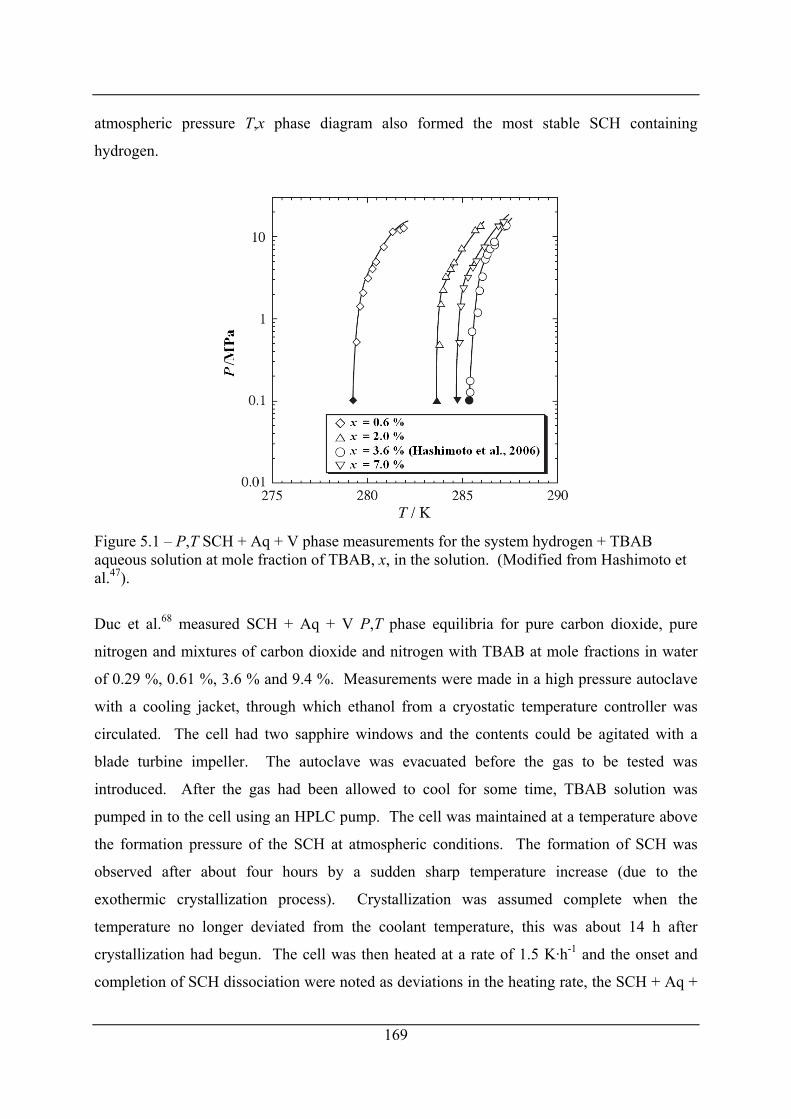
atmospheric pressure T,x phase diagram also formed the most stable SCH containing
hydrogen.
Figure 5.1 – P,T SCH + Aq + V phase measurements for the system hydrogen + TBAB aqueous solution at mole fraction of TBAB, x, in the solution. (Modified from Hashimoto et al.47).
Duc et al.68 measured SCH + Aq + V P,T phase equilibria for pure carbon dioxide, pure
nitrogen and mixtures of carbon dioxide and nitrogen with TBAB at mole fractions in water
of 0.29 %, 0.61 %, 3.6 % and 9.4 %. Measurements were made in a high pressure autoclave
with a cooling jacket, through which ethanol from a cryostatic temperature controller was
circulated. The cell had two sapphire windows and the contents could be agitated with a
blade turbine impeller. The autoclave was evacuated before the gas to be tested was
introduced. After the gas had been allowed to cool for some time, TBAB solution was
pumped in to the cell using an HPLC pump. The cell was maintained at a temperature above
the formation pressure of the SCH at atmospheric conditions. The formation of SCH was
observed after about four hours by a sudden sharp temperature increase (due to the
exothermic crystallization process). Crystallization was assumed complete when the
temperature no longer deviated from the coolant temperature, this was about 14 h after
crystallization had begun. The cell was then heated at a rate of 1.5 K·h-1 and the onset and
completion of SCH dissociation were noted as deviations in the heating rate, the SCH + Aq +
169
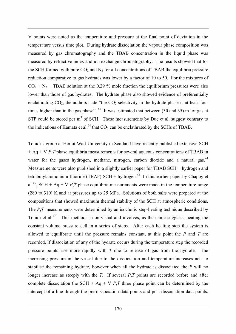
170
V points were noted as the temperature and pressure at the final point of deviation in the
temperature versus time plot. During hydrate dissociation the vapour phase composition was
measured by gas chromatography and the TBAB concentration in the liquid phase was
measured by refractive index and ion exchange chromatography. The results showed that for
the SCH formed with pure CO2 and N2 for all concentrations of TBAB the equilibria pressure
reduction comparative to gas hydrates was lower by a factor of 10 to 50. For the mixtures of
CO2 + N2 + TBAB solution at the 0.29 % mole fraction the equilibrium pressures were also
lower than those of gas hydrates. The hydrate phase also showed evidence of preferentially
enclathrating CO2, the authors state “the CO2 selectivity in the hydrate phase is at least four
times higher than in the gas phase”. 68 It was estimated that between (30 and 35) m3 of gas at
STP could be stored per m3 of SCH. These measurements by Duc et al. suggest contrary to
the indications of Kamata et al.64 that CO2 can be enclathrated by the SCHs of TBAB.
Tohidi’s group at Heriot Watt University in Scotland have recently published extensive SCH
+ Aq + V P,T phase equilibria measurements for several aqueous concentrations of TBAB in
water for the gases hydrogen, methane, nitrogen, carbon dioxide and a natural gas.44
Measurements were also published in a slightly earlier paper for TBAB SCH + hydrogen and
tetrabutylammonium fluoride (TBAF) SCH + hydrogen.45 In this earlier paper by Chapoy et
al.45, SCH + Aq + V P,T phase equilibria measurements were made in the temperature range
(280 to 310) K and at pressures up to 25 MPa. Solutions of both salts were prepared at the
compositions that showed maximum thermal stability of the SCH at atmospheric conditions.
The P,T measurements were determined by an isochoric step-heating technique described by
Tohidi et al.170 This method is non-visual and involves, as the name suggests, heating the
constant volume pressure cell in a series of steps. After each heating step the system is
allowed to equilibrate until the pressure remains constant, at this point the P and T are
recorded. If dissociation of any of the hydrate occurs during the temperature step the recorded
pressure points rise more rapidly with T due to release of gas from the hydrate. The
increasing pressure in the vessel due to the dissociation and temperature increases acts to
stabilise the remaining hydrate, however when all the hydrate is dissociated the P will no
longer increase as steeply with the T. If several P,T points are recorded before and after
complete dissociation the SCH + Aq + V P,T three phase point can be determined by the
intercept of a line through the pre-dissociation data points and post-dissociation data points.
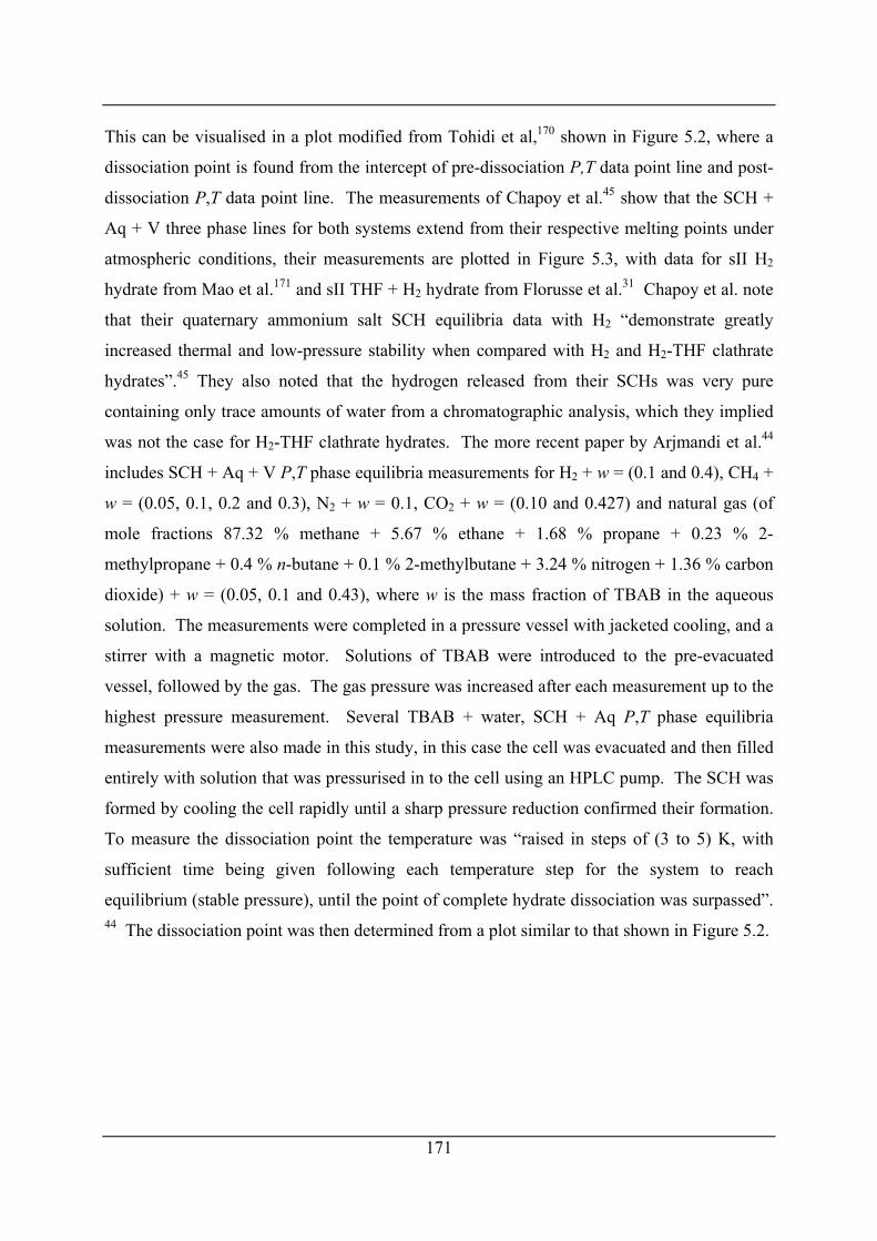
171
This can be visualised in a plot modified from Tohidi et al,170 shown in Figure 5.2, where a
dissociation point is found from the intercept of pre-dissociation P,T data point line and post-
dissociation P,T data point line. The measurements of Chapoy et al.45 show that the SCH +
Aq + V three phase lines for both systems extend from their respective melting points under
atmospheric conditions, their measurements are plotted in Figure 5.3, with data for sII H2
hydrate from Mao et al.171 and sII THF + H2 hydrate from Florusse et al.31 Chapoy et al. note
that their quaternary ammonium salt SCH equilibria data with H2 “demonstrate greatly
increased thermal and low-pressure stability when compared with H2 and H2-THF clathrate
hydrates”.45 They also noted that the hydrogen released from their SCHs was very pure
containing only trace amounts of water from a chromatographic analysis, which they implied
was not the case for H2-THF clathrate hydrates. The more recent paper by Arjmandi et al.44
includes SCH + Aq + V P,T phase equilibria measurements for H2 + w = (0.1 and 0.4), CH4 +
w = (0.05, 0.1, 0.2 and 0.3), N2 + w = 0.1, CO2 + w = (0.10 and 0.427) and natural gas (of
mole fractions 87.32 % methane + 5.67 % ethane + 1.68 % propane + 0.23 % 2-
methylpropane + 0.4 % n-butane + 0.1 % 2-methylbutane + 3.24 % nitrogen + 1.36 % carbon
dioxide) + w = (0.05, 0.1 and 0.43), where w is the mass fraction of TBAB in the aqueous
solution. The measurements were completed in a pressure vessel with jacketed cooling, and a
stirrer with a magnetic motor. Solutions of TBAB were introduced to the pre-evacuated
vessel, followed by the gas. The gas pressure was increased after each measurement up to the
highest pressure measurement. Several TBAB + water, SCH + Aq P,T phase equilibria
measurements were also made in this study, in this case the cell was evacuated and then filled
entirely with solution that was pressurised in to the cell using an HPLC pump. The SCH was
formed by cooling the cell rapidly until a sharp pressure reduction confirmed their formation.
To measure the dissociation point the temperature was “raised in steps of (3 to 5) K, with
sufficient time being given following each temperature step for the system to reach
equilibrium (stable pressure), until the point of complete hydrate dissociation was surpassed”. 44 The dissociation point was then determined from a plot similar to that shown in Figure 5.2.
Figure 5.2 – Dissociation point determination from pre-dissociation point P,T measurements and post-dissociation point P,T measurements. (Modified from Tohidi et al.170).
Figure 5.3 – Measurements of dissociation conditions of H2+ TBAB SCH and H2 + TBAF SCH, also plotted are data for pure H2 sII hydrate and H2 + THF sII hydrate. a H2 sII hydrate data from Mao et al.171 b H2 + THF sII hydrate data from Florusse et al.31 (Modified from Chapoy et al.45).
172
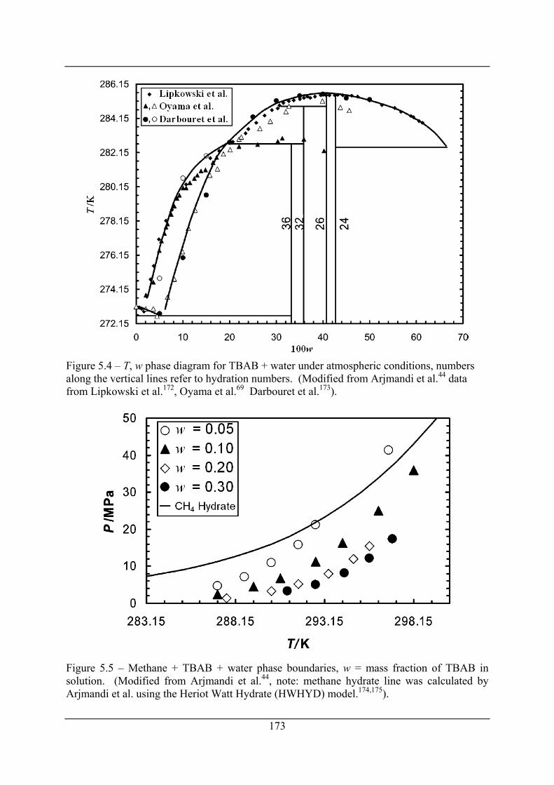
Figure 5.4 – T, w phase diagram for TBAB + water under atmospheric conditions, numbers along the vertical lines refer to hydration numbers. (Modified from Arjmandi et al.44 data from Lipkowski et al.172, Oyama et al.69 Darbouret et al.173).
Figure 5.5 – Methane + TBAB + water phase boundaries, w = mass fraction of TBAB in solution. (Modified from Arjmandi et al.44, note: methane hydrate line was calculated by Arjmandi et al. using the Heriot Watt Hydrate (HWHYD) model.174,175).
173
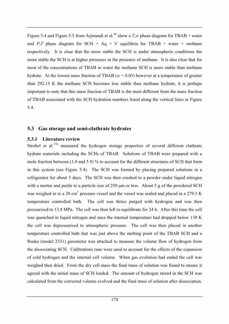
174
Figure 5.4 and Figure 5.5 from Arjmandi et al.44 show a T,w phase diagram for TBAB + water
and P,T phase diagram for SCH + Aq + V equilibria for TBAB + water + methane
respectively. It is clear that the more stable the SCH is under atmospheric conditions the
more stable the SCH is at higher pressures in the presence of methane. It is also clear that for
most of the concentrations of TBAB in water the methane SCH is more stable than methane
hydrate. At the lowest mass fraction of TBAB (w = 0.05) however at a temperature of greater
than 292.15 K the methane SCH becomes less stable than methane hydrate, it is perhaps
important to note that this mass fraction of TBAB is the most different from the mass fraction
of TBAB associated with the SCH hydration numbers listed along the vertical lines in Figure
5.4.
5.3 Gas storage and semi-clathrate hydrates
5.3.1 Literature review Strobel et al.176 measured the hydrogen storage properties of several different clathrate
hydrate materials including the SCHs of TBAB. Solutions of TBAB were prepared with a
mole fraction between (1.0 and 5.9) % to account for the different structures of SCH that form
in this system (see Figure 5.4). The SCH was formed by placing prepared solutions in a
refrigerator for about 3 days. The SCH was then crushed to a powder under liquid nitrogen
with a mortar and pestle to a particle size of 250 μm or less. About 5 g of the powdered SCH
was weighed in to a 20 cm3 pressure vessel and the vessel was sealed and placed in a 279.5 K
temperature controlled bath. The cell was thrice purged with hydrogen and was then
pressurized to 13.8 MPa. The cell was then left to equilibrate for 24 h. After this time the cell
was quenched in liquid nitrogen and once the internal temperature had dropped below 130 K
the cell was depressurised to atmospheric pressure. The cell was then placed in another
temperature controlled bath that was just above the melting point of the TBAB SCH and a
Ruska (model 2331) gasometer was attached to measure the volume flow of hydrogen from
the dissociating SCH. Calibrations runs were used to account for the effects of the expansion
of cold hydrogen and the internal cell volume. When gas evolution had ended the cell was
weighed then dried. From the dry cell mass the final mass of solution was found to ensure it
agreed with the initial mass of SCH loaded. The amount of hydrogen stored in the SCH was
calculated from the corrected volume evolved and the final mass of solution after dissociation.
The results of the measurements are shown in Figure 5.6, where the bulk mass fraction of
hydrogen stored (“not corrected for stoichiometry or contributions from multiple semi-
clathrate phases present”) is plotted as a function of the mole fraction of TBAB in the solution
used to prepare the SCH. Strobel et al. noted the maximum hydrogen storage mass fraction of
0.241 % was at the mole fraction of TBAB in the solution of 2.71 %, which corresponds
closely to the stoichiometry of the most recently discovered SCH of TBAB·38H2O (by
Shimada et al.62), in which the mole fraction of TBAB is 2.56 %. (note: the hydration number
of this SCH is not shown on Figure 5.4).
Figure 5.6 – Bulk mass fraction of hydrogen, wH2, stored as a function of the TBAB mole fraction, xTBAB, in the solution used to prepare the SCH. (Modified from Strobel et al.176).
The work of Strobel et al.176 suggests that the mass fraction of hydrogen stored in the SCH of
TBAB was only as high as 0.214 %, just over a third of the calculated value assuming full
occupation (by one hydrogen molecule) of 0.597 % in the TBAB·38H2O structure. It is
interesting to note however that McMullan et al.61, Jeffrey4, Davidson11 and Shimada et al. 63
observed that air was enclathrated in their SCHs that they studied at atmospheric pressure. In
the experiments of Strobel et al.176 there were no apparent steps, such as evacuation, that
would lead to the removal molecules of air (N2, O2, and Ar) from the SCH, this may have lead
to an underestimation of the amount of hydrogen that could be stored in the TBAB SCH.
175
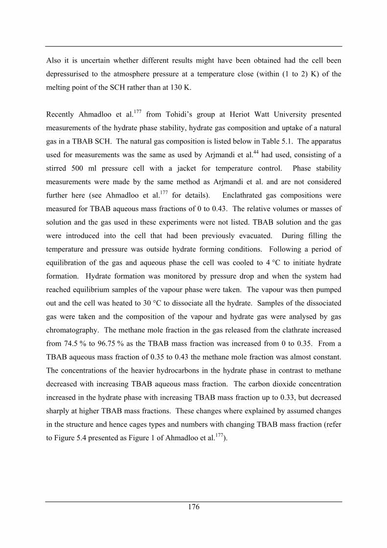
176
Also it is uncertain whether different results might have been obtained had the cell been
depressurised to the atmosphere pressure at a temperature close (within (1 to 2) K) of the
melting point of the SCH rather than at 130 K.
Recently Ahmadloo et al.177 from Tohidi’s group at Heriot Watt University presented
measurements of the hydrate phase stability, hydrate gas composition and uptake of a natural
gas in a TBAB SCH. The natural gas composition is listed below in Table 5.1. The apparatus
used for measurements was the same as used by Arjmandi et al.44 had used, consisting of a
stirred 500 ml pressure cell with a jacket for temperature control. Phase stability
measurements were made by the same method as Arjmandi et al. and are not considered
further here (see Ahmadloo et al.177 for details). Enclathrated gas compositions were
measured for TBAB aqueous mass fractions of 0 to 0.43. The relative volumes or masses of
solution and the gas used in these experiments were not listed. TBAB solution and the gas
were introduced into the cell that had been previously evacuated. During filling the
temperature and pressure was outside hydrate forming conditions. Following a period of
equilibration of the gas and aqueous phase the cell was cooled to 4 °C to initiate hydrate
formation. Hydrate formation was monitored by pressure drop and when the system had
reached equilibrium samples of the vapour phase were taken. The vapour was then pumped
out and the cell was heated to 30 °C to dissociate all the hydrate. Samples of the dissociated
gas were taken and the composition of the vapour and hydrate gas were analysed by gas
chromatography. The methane mole fraction in the gas released from the clathrate increased
from 74.5 % to 96.75 % as the TBAB mass fraction was increased from 0 to 0.35. From a
TBAB aqueous mass fraction of 0.35 to 0.43 the methane mole fraction was almost constant.
The concentrations of the heavier hydrocarbons in the hydrate phase in contrast to methane
decreased with increasing TBAB aqueous mass fraction. The carbon dioxide concentration
increased in the hydrate phase with increasing TBAB mass fraction up to 0.33, but decreased
sharply at higher TBAB mass fractions. These changes where explained by assumed changes
in the structure and hence cages types and numbers with changing TBAB mass fraction (refer
to Figure 5.4 presented as Figure 1 of Ahmadloo et al.177).
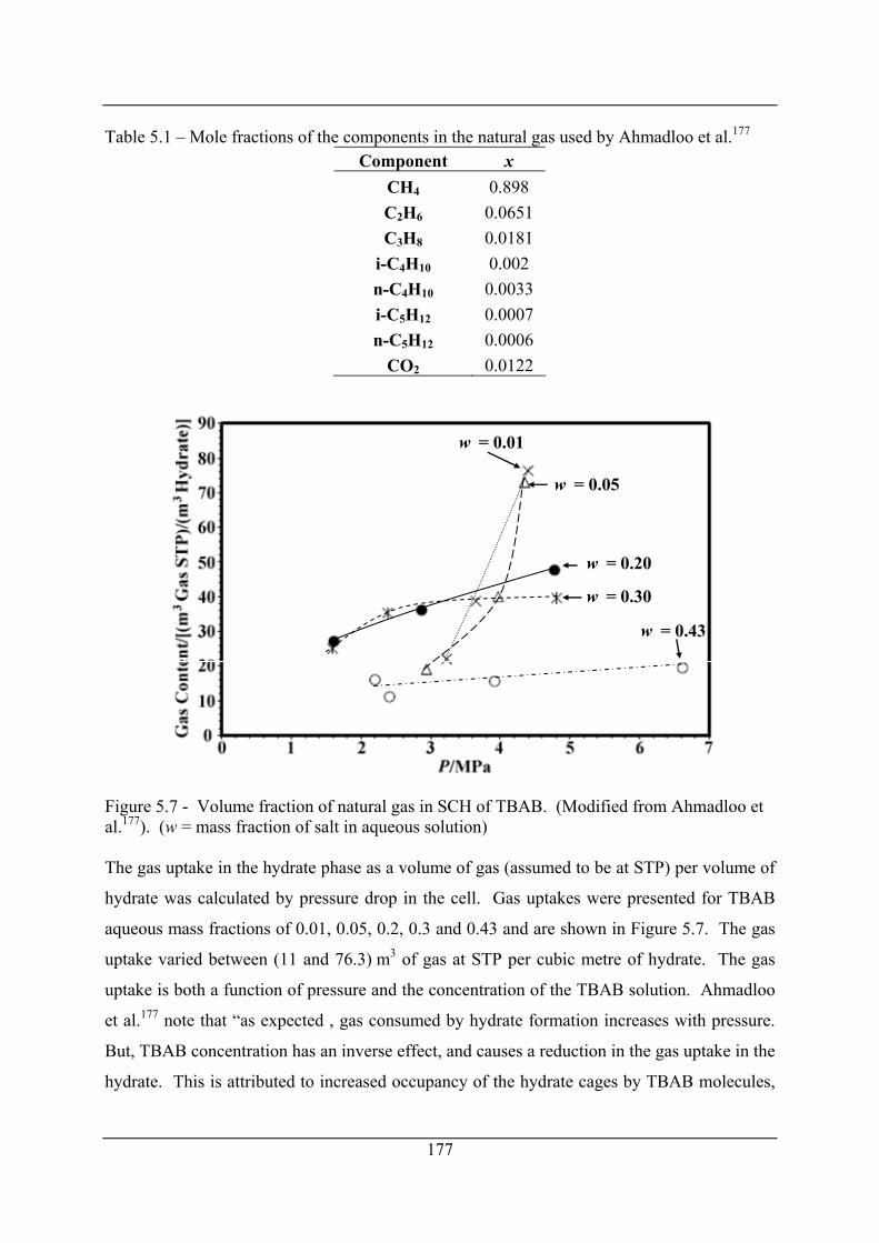
Table 5.1 – Mole fractions of the components in the natural gas used by Ahmadloo et al.177 Component x
CH4 0.898 C2H6 0.0651 C3H8 0.0181
i-C4H10 0.002 n-C4H10 0.0033 i-C5H12 0.0007 n-C5H12 0.0006
CO2 0.0122
w = 0.05
w = 0.20
w = 0.30
w = 0.43
w = 0.01
Figure 5.7 - Volume fraction of natural gas in SCH of TBAB. (Modified from Ahmadloo et al.177). (w = mass fraction of salt in aqueous solution) The gas uptake in the hydrate phase as a volume of gas (assumed to be at STP) per volume of
hydrate was calculated by pressure drop in the cell. Gas uptakes were presented for TBAB
aqueous mass fractions of 0.01, 0.05, 0.2, 0.3 and 0.43 and are shown in Figure 5.7. The gas
uptake varied between (11 and 76.3) m3 of gas at STP per cubic metre of hydrate. The gas
uptake is both a function of pressure and the concentration of the TBAB solution. Ahmadloo
et al.177 note that “as expected , gas consumed by hydrate formation increases with pressure.
But, TBAB concentration has an inverse effect, and causes a reduction in the gas uptake in the
hydrate. This is attributed to increased occupancy of the hydrate cages by TBAB molecules,
177
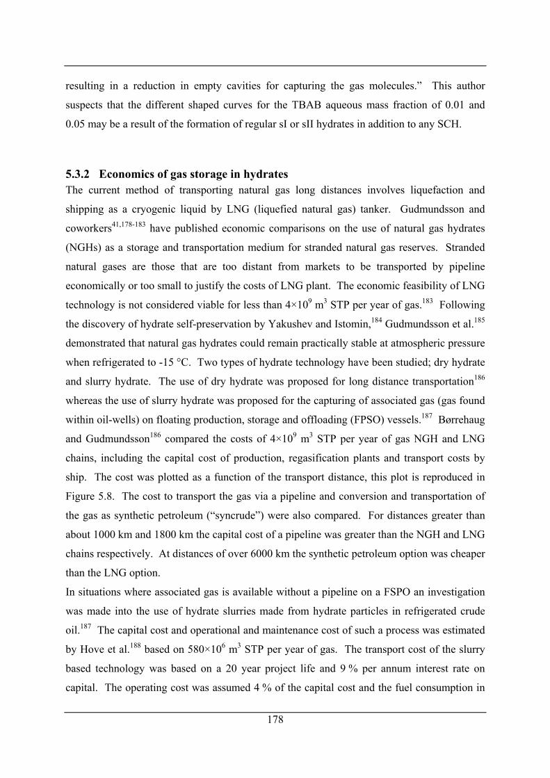
178
resulting in a reduction in empty cavities for capturing the gas molecules.” This author
suspects that the different shaped curves for the TBAB aqueous mass fraction of 0.01 and
0.05 may be a result of the formation of regular sI or sII hydrates in addition to any SCH.
5.3.2 Economics of gas storage in hydrates The current method of transporting natural gas long distances involves liquefaction and
shipping as a cryogenic liquid by LNG (liquefied natural gas) tanker. Gudmundsson and
coworkers41,178-183 have published economic comparisons on the use of natural gas hydrates
(NGHs) as a storage and transportation medium for stranded natural gas reserves. Stranded
natural gases are those that are too distant from markets to be transported by pipeline
economically or too small to justify the costs of LNG plant. The economic feasibility of LNG
technology is not considered viable for less than 4×10⁹ m3 STP per year of gas.183 Following
the discovery of hydrate self-preservation by Yakushev and Istomin,184 Gudmundsson et al.185
demonstrated that natural gas hydrates could remain practically stable at atmospheric pressure
when refrigerated to -15 °C. Two types of hydrate technology have been studied; dry hydrate
and slurry hydrate. The use of dry hydrate was proposed for long distance transportation186
whereas the use of slurry hydrate was proposed for the capturing of associated gas (gas found
within oil-wells) on floating production, storage and offloading (FPSO) vessels.187 Børrehaug
and Gudmundsson186 compared the costs of 4×10⁹ m3 STP per year of gas NGH and LNG
chains, including the capital cost of production, regasification plants and transport costs by
ship. The cost was plotted as a function of the transport distance, this plot is reproduced in
Figure 5.8. The cost to transport the gas via a pipeline and conversion and transportation of
the gas as synthetic petroleum (“syncrude”) were also compared. For distances greater than
about 1000 km and 1800 km the capital cost of a pipeline was greater than the NGH and LNG
chains respectively. At distances of over 6000 km the synthetic petroleum option was cheaper
than the LNG option.
In situations where associated gas is available without a pipeline on a FSPO an investigation
was made into the use of hydrate slurries made from hydrate particles in refrigerated crude
oil.187 The capital cost and operational and maintenance cost of such a process was estimated
by Hove et al.188 based on 580×106 m3 STP per year of gas. The transport cost of the slurry
based technology was based on a 20 year project life and 9 % per annum interest rate on
capital. The operating cost was assumed 4 % of the capital cost and the fuel consumption in
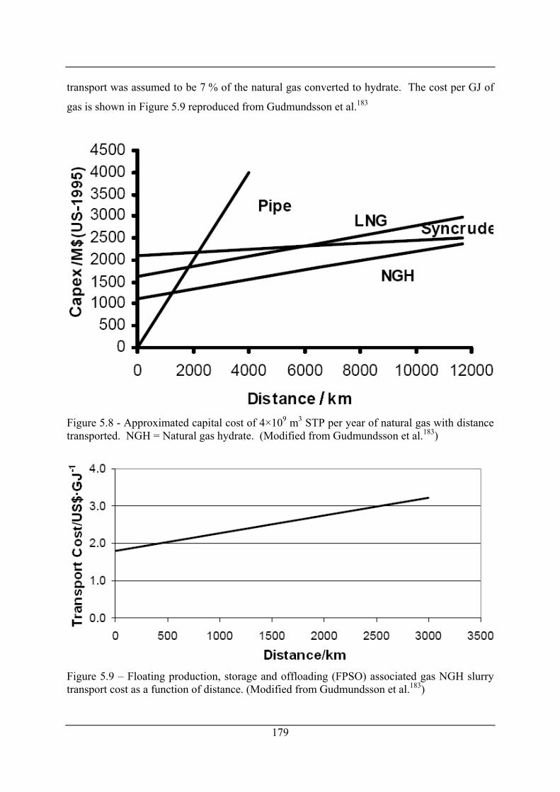
transport was assumed to be 7 % of the natural gas converted to hydrate. The cost per GJ of
gas is shown in Figure 5.9 reproduced from Gudmundsson et al.183
Figure 5.8 - Approximated capital cost of 4×10⁹ m3 STP per year of natural gas with distance transported. NGH = Natural gas hydrate. (Modified from Gudmundsson et al.183)
Figure 5.9 – Floating production, storage and offloading (FPSO) associated gas NGH slurry transport cost as a function of distance. (Modified from Gudmundsson et al.183)
179
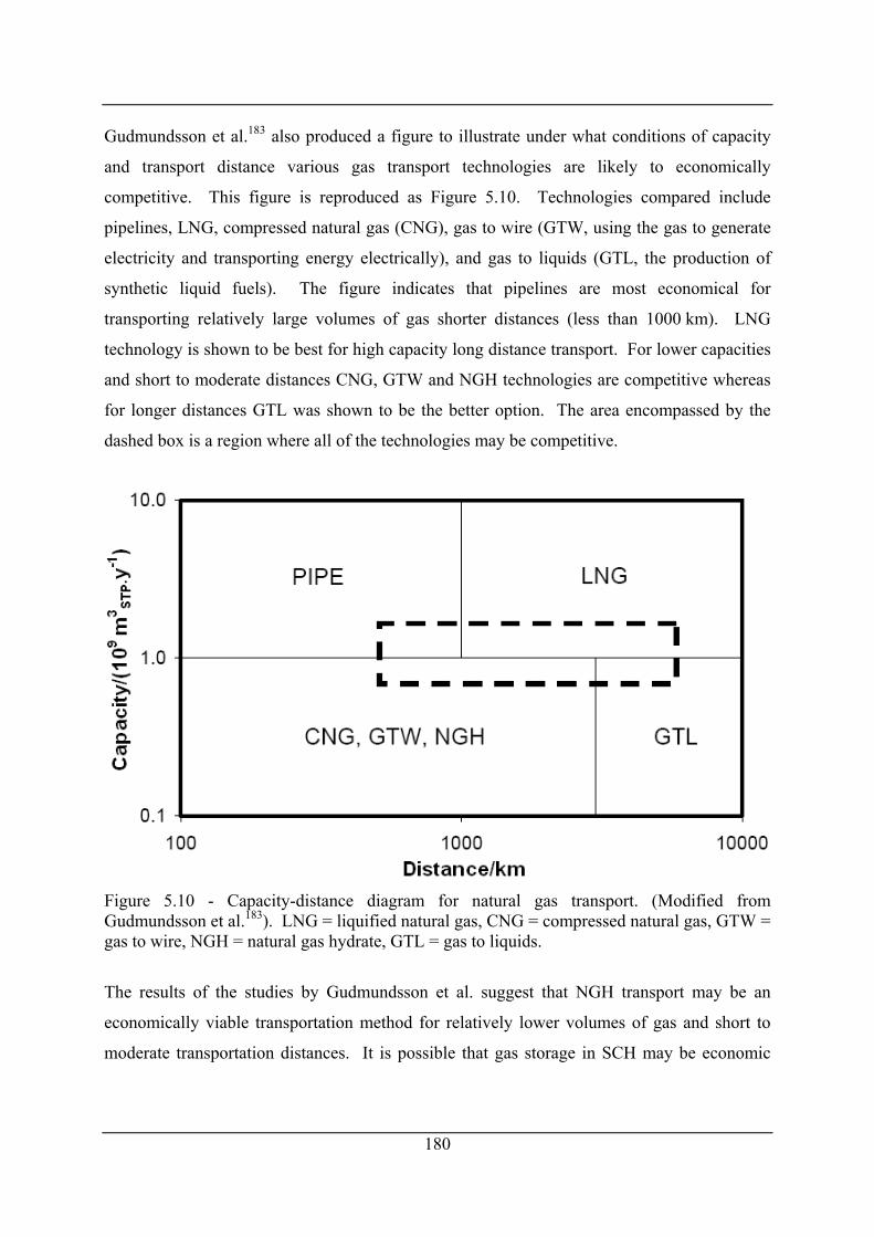
Gudmundsson et al.183 also produced a figure to illustrate under what conditions of capacity
and transport distance various gas transport technologies are likely to economically
competitive. This figure is reproduced as Figure 5.10. Technologies compared include
pipelines, LNG, compressed natural gas (CNG), gas to wire (GTW, using the gas to generate
electricity and transporting energy electrically), and gas to liquids (GTL, the production of
synthetic liquid fuels). The figure indicates that pipelines are most economical for
transporting relatively large volumes of gas shorter distances (less than 1000 km). LNG
technology is shown to be best for high capacity long distance transport. For lower capacities
and short to moderate distances CNG, GTW and NGH technologies are competitive whereas
for longer distances GTL was shown to be the better option. The area encompassed by the
dashed box is a region where all of the technologies may be competitive.
Figure 5.10 - Capacity-distance diagram for natural gas transport. (Modified from Gudmundsson et al.183). LNG = liquified natural gas, CNG = compressed natural gas, GTW = gas to wire, NGH = natural gas hydrate, GTL = gas to liquids.
The results of the studies by Gudmundsson et al. suggest that NGH transport may be an
economically viable transportation method for relatively lower volumes of gas and short to
moderate transportation distances. It is possible that gas storage in SCH may be economic
180
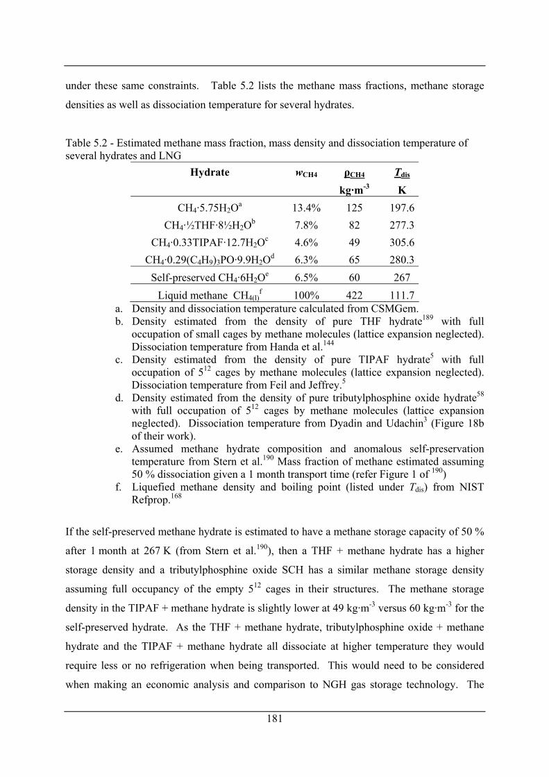
181
under these same constraints. Table 5.2 lists the methane mass fractions, methane storage
densities as well as dissociation temperature for several hydrates.
Table 5.2 - Estimated methane mass fraction, mass density and dissociation temperature of several hydrates and LNG
Hydrate wCH4 ρCH4 Tdis
kg·m-3 K CH4·5.75H2Oa 13.4% 125 197.6
CH4·½THF·8½H2Ob 7.8% 82 277.3 CH4·0.33TIPAF·12.7H2Oc 4.6% 49 305.6
CH4·0.29(C4H9)3PO·9.9H2Od 6.3% 65 280.3 Self-preserved CH4·6H2Oe 6.5% 60 267
Liquid methane CH4(l)f 100% 422 111.7
a. Density and dissociation temperature calculated from CSMGem. b. Density estimated from the density of pure THF hydrate189 with full
occupation of small cages by methane molecules (lattice expansion neglected). Dissociation temperature from Handa et al.144
c. Density estimated from the density of pure TIPAF hydrate5 with full occupation of 512 cages by methane molecules (lattice expansion neglected). Dissociation temperature from Feil and Jeffrey.5
d. Density estimated from the density of pure tributylphosphine oxide hydrate58 with full occupation of 512 cages by methane molecules (lattice expansion neglected). Dissociation temperature from Dyadin and Udachin3 (Figure 18b of their work).
e. Assumed methane hydrate composition and anomalous self-preservation temperature from Stern et al.190 Mass fraction of methane estimated assuming 50 % dissociation given a 1 month transport time (refer Figure 1 of 190)
f. Liquefied methane density and boiling point (listed under Tdis) from NIST Refprop.168
If the self-preserved methane hydrate is estimated to have a methane storage capacity of 50 %
after 1 month at 267 K (from Stern et al.190), then a THF + methane hydrate has a higher
storage density and a tributylphosphine oxide SCH has a similar methane storage density
assuming full occupancy of the empty 512 cages in their structures. The methane storage
density in the TIPAF + methane hydrate is slightly lower at 49 kg·m-3 versus 60 kg·m-3 for the
self-preserved hydrate. As the THF + methane hydrate, tributylphosphine oxide + methane
hydrate and the TIPAF + methane hydrate all dissociate at higher temperature they would
require less or no refrigeration when being transported. This would need to be considered
when making an economic analysis and comparison to NGH gas storage technology. The
182
more boil off or dissociation of gas from the hydrate the more recompression and cooling is
needed. The chemical cost of the salt or promoter (THF) would need to be considered. For
the THF + methane hydrate some THF might be lost to the gas phase during dissociation. For
the SCH forming salts there should be no or negligible vaporisation of the salt. The salt
chemical cost could thus be considered a capital cost. The THF cost would be both an initial
capital cost and an operating cost for the fraction lost to vapour phase.
5.4 Experimental Pressure-temperature measurements of SCH + Aq + V phase equilibria of the
tetraisopentylammonium fluoride (TIPAF) + water + methane system were the primary focus
of the experimental work. The salt TIPAF was selected as the SCH TIPAF·38H2O has both a
relatively high melting point (Feil and Jeffrey5 give a melting point of 31.2 °C and Lipkowski
et al.67 give a value of 32.4 °C) as well as a high fraction of unoccupied cages comparable to
other SCH (3 unoccupied cages per molecule of salt, see Chapter 1 section 1.6.2). TIPAF
however was not available commercially and so was prepared from triisopentylamine,
isopentyl bromide and silver fluoride, this preparation is described in the materials section
below. The concentration of TIPAF was fixed for the phase equilibria measurements by the
crystallisation of the SCH from an aqueous solution of the salt. The hydration number of the
crystallised SCH was determined experimentally by Karl Fischer titration for the water
content.
5.4.1 Materials Methane was sourced from Linde Gas, U.K Ltd, with a purity of 99.975%, this was used
without further purification.
Tetraisopentylammonium fluoride was prepared from triisopentylamine, isopentyl bromide
and silver fluoride. The purities and sources of the chemicals used in the preparation and
purification steps are listed in Table 5.3. The first step was the preparation of
tetraisopentylammonium bromide (TIPAB). Lipkowski et al.67 prepared TIPAB by refluxing
triisopentylamine and isopentyl bromide in acetonitrile by the Menshutkin reaction, eq (5.1).
The same method was used in this work, approximately 78.2 g (0.344 mol) of
triisopentylamine, 86.4 g (0.572 mol) of isopentyl bromide and 97.6 g (2.38 mol) of
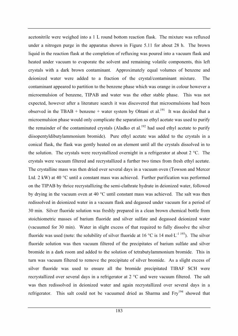
183
acetonitrile were weighed into a 1 L round bottom reaction flask. The mixture was refluxed
under a nitrogen purge in the apparatus shown in Figure 5.11 for about 28 h. The brown
liquid in the reaction flask at the completion of refluxing was poured into a vacuum flask and
heated under vacuum to evaporate the solvent and remaining volatile components, this left
crystals with a dark brown contaminant. Approximately equal volumes of benzene and
deionized water were added to a fraction of the crystal/contaminant mixture. The
contaminant appeared to partition to the benzene phase which was orange in colour however a
microemulsion of benzene, TIPAB and water was the other stable phase. This was not
expected, however after a literature search it was discovered that microemulsions had been
observed in the TBAB + benzene + water system by Ohtani et al.191 It was decided that a
microemulsion phase would only complicate the separation so ethyl acetate was used to purify
the remainder of the contaminated crystals (Aladko et al.192 had used ethyl acetate to purify
diisopentyldibutylammonium bromide). Pure ethyl acetate was added to the crystals in a
conical flask, the flask was gently heated on an element until all the crystals dissolved in to
the solution. The crystals were recrystallized overnight in a refrigerator at about 2 °C. The
crystals were vacuum filtered and recrystallized a further two times from fresh ethyl acetate.
The crystalline mass was then dried over several days in a vacuum oven (Towson and Mercer
Ltd. 2 kW) at 40 °C until a constant mass was achieved. Further purification was performed
on the TIPAB by thrice recrystallizing the semi-clathrate hydrate in deionized water, followed
by drying in the vacuum oven at 40 °C until constant mass was achieved. The salt was then
redissolved in deionized water in a vacuum flask and degassed under vacuum for a period of
30 min. Silver fluoride solution was freshly prepared in a clean brown chemical bottle from
stoichiometric masses of barium fluoride and silver sulfate and degassed deionized water
(vacuumed for 30 min). Water in slight excess of that required to fully dissolve the silver
fluoride was used (note: the solubility of silver fluoride at 16 °C is 14 mol·L-1 193). The silver
fluoride solution was then vacuum filtered of the precipitates of barium sulfate and silver
bromide in a dark room and added to the solution of tetrabutylammonium bromide. This in
turn was vacuum filtered to remove the precipitate of silver bromide. As a slight excess of
silver fluoride was used to ensure all the bromide precipitated TIBAF SCH were
recrystallized over several days in a refrigerator at 2 °C and were vacuum filtered. The salt
was then redissolved in deionized water and again recrystallized over several days in a
refrigerator. This salt could not be vacuumed dried as Sharma and Fry194 showed that
tetraalkylammonium fluorides are unstable unless in the presence of at least three waters of
hydration.
(5.1)
(5.2)
Table 5.3 – Chemical purities for preparation and purification of TIPAF. Chemical Supplier Purity
Triisopentylamine Fluka, technical grade ≥90 % Isopentyl bromide Aldrich 96 %
Acetonitrile JT Baker, ACS reagent 99.5 % Silver sulfate Merck, Analysis grade ACS 98.5 %
Barium fluoride Sigma Aldrich, <5 microns 98 % Benzene BDH, HPLC grade 99.8 %
Ethyl acetate BDH, HPLC grade 99.8 % Nitrogen BOC gases, oxygen free -
Samples of the TIPAF SCH were analysed by proton NMR in tetra-deuterated methanol
(Cambridge isotope laboratories, 99.8%) to investigate the purity of the SCH. A sample of
11.8 mg of the TIPAF SCH was added to 267.5 mg of deuterated methanol (CD3OD) in a 3
mm NMR tube. The spectrum was recorded on the University of Canterbury Chemistry
departments’ Varian VNMR 500 MHz spectrometer at an ambient temperature of 23 °C, and
is shown in Figure 5.12. The chemical shifts of the TIPAF peaks are listed in Table 5.4, they
are similar to those published by Harmon et al.104 presented in Chapter 2 for
tetraisopentylammonium iodide in D2O (see Table 2.2). They are also similar to the
comparable peaks for the tetrahexylammonium ion (see Figure 2.22), the chemical shift of the
methylene hydrogens labelled 1 on both ions resonate within 0.07 ppm and the number 2
methylene hydrogens resonate within 0.02 ppm. If triisopentylamine was a contaminant in
TIPAF the only distinguishable peak would be that on the first methylene group off the
184
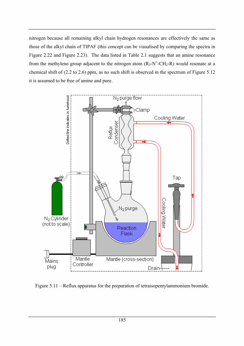
nitrogen because all remaining alkyl chain hydrogen resonances are effectively the same as
those of the alkyl chain of TIPAF (this concept can be visualised by comparing the spectra in
Figure 2.22 and Figure 2.23). The data listed in Table 2.1 suggests that an amine resonance
from the methylene group adjacent to the nitrogen atom (R3-N+-CH2-R) would resonate at a
chemical shift of (2.2 to 2.6) ppm, as no such shift is observed in the spectrum of Figure 5.12
it is assumed to be free of amine and pure.
Figure 5.11 – Reflux apparatus for the preparation of tetraisopentylammonium bromide.
185
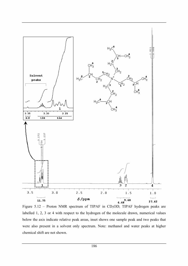
Figure 5.12 – Proton NMR spectrum of TIPAF in CD3OD; TIPAF hydrogen peaks are
labelled 1, 2, 3 or 4 with respect to the hydrogen of the molecule drawn, numerical values
below the axis indicate relative peak areas, inset shows one sample peak and two peaks that
were also present in a solvent only spectrum. Note: methanol and water peaks at higher
chemical shift are not shown.
186
187
Table 5.4 – Proton NMR chemical shifts and calculated hydrogen atoms for each shift/peak Resonating hydrogen
(in bold) Label in
Figure 5.12Chemical shift
δ/ppm Hydrogens from
peak area* Actual
hydrogens N+[CH2CH2CH(CH3)2]4 1 3.25 8.2 8 N+[CH2CH2CH(CH3)2]4 2 1.55 8.3 8 N+[CH2CH2CH(CH3)2]4 3 1.67 3.8 4 N+[CH2CH2CH(CH3)2]4 4 1.00 23.6 24 * Calculated from fraction of total area for TIPAF peaks multiplied by 44 (the number of hydrogen atoms in a TIPAF molecule)
5.4.2 Preparation of tetraisopentylammonium fluoride + water at fixed concentration
The mole fraction of TIPAF in water for the P,T phase equilibria experiments was fixed by
crystallizing a SCH of known hydration number. The TIPAF SCH with hydration number of
38 was desired as it has the highest melting point and the literature suggests that the SCH with
the highest melting point forms the most stable SCH with gases. A dilute solution of TIPAF
in water was prepared from crystals of TIPAF SCH by dissolving them in warm deionised
water. A sample of this solution was analysed by Karl Fischer titration for water content
using an automatic volumetric Karl Fischer (KF) titrator (Radiometer Analytical TIM550
Titralab). Methanol (BDH HPLC grade 99.8 %) was weighed on a balance (Mettler AE200,
± 0.0005 g half resolution) in to a septum bottle that had been prior flushed with dry nitrogen
and the rubber bung cap was immediately placed on the bottle. A 1 mL syringe was tared on
the balance and was then used to remove a methanol sample of between (0.2 and 0.4) mL
from the septum bottle, this sample was then weighed on the balance. The sample was then
injected in to the KF titrator and the start button was pressed to begin the titration. Before the
titration began the KF titrator had been allowed to stabilize for several hours and was
calibrated using a standard solution of mass fraction 1 % water (Merck Apura water standard
1 % for volumetric KF titration). The mass of methanol injected was entered at the prompting
of the KF titrator’s controller and the titrator calculated from the volume of titrant (Merck
Combitrant 5) required the mass fraction of water in the sample. This analysis was repeated
10 times and an averaged value of the methanol water content was calculated as a mass
fraction of (0.157 ± 0.006) % (where the uncertainty was calculated by a student-t 95 %
confidence interval). The bottle of methanol was then reweighed and TIPAF solution was

188
injected by syringe in to the bottle on the balance, so that the mass of solution added was
known. The bottle was shaken to mix the injected solution. Ten different samples of known
mass (between (0.2 and 0.4)g) of the methanol + TIPAF + water solution were then analysed
using the KF titrator. The concentration of water in the solution was calculated by
considering the amount of water in the methanol and the relative masses of solution and
methanol in the mixture. The mass fraction of TIPAF was calculated as (3.15 ± 0.12) %
where the uncertainty was calculated by a student-t 95 % confidence interval. From Figure
1.6 this mass fraction of salt in solution should result in the crystallization of a SCH with a
structural hydration number of 38. The dilute TIPAF solution was placed in a refrigerator at
approximately 2 °C and crystallization of SCH was allowed to occur over 2 days. The
solution containing SCH crystals was then vacuum filtered and the crystalline mass of about
25 g was gently squeezed between two large diameter (150 mm) sheets of absorbent filter
paper. The procedure outlined above to measure the water content of methanol was then
repeated with a different sample of methanol. A known mass of the SCH crystals (about 1 g)
were added to known mass of methanol, dry nitrogen was flushed around the top of the
septum bottle as soon as the crystals were added and the then septum bottle was resealed with
the rubber bung. The SCH crystals were dissolved in the solution by gentle shaking and then
10 samples of the solution were tested using the KF titrator. The results indicate a mass
fraction of TIPAF in the SCH crystals of (31.49 ± 0.38) %, which equates to a hydration
number of 38.3 ± 0.7 (where the uncertainties were calculated by a student-t 95 % confidence
interval).
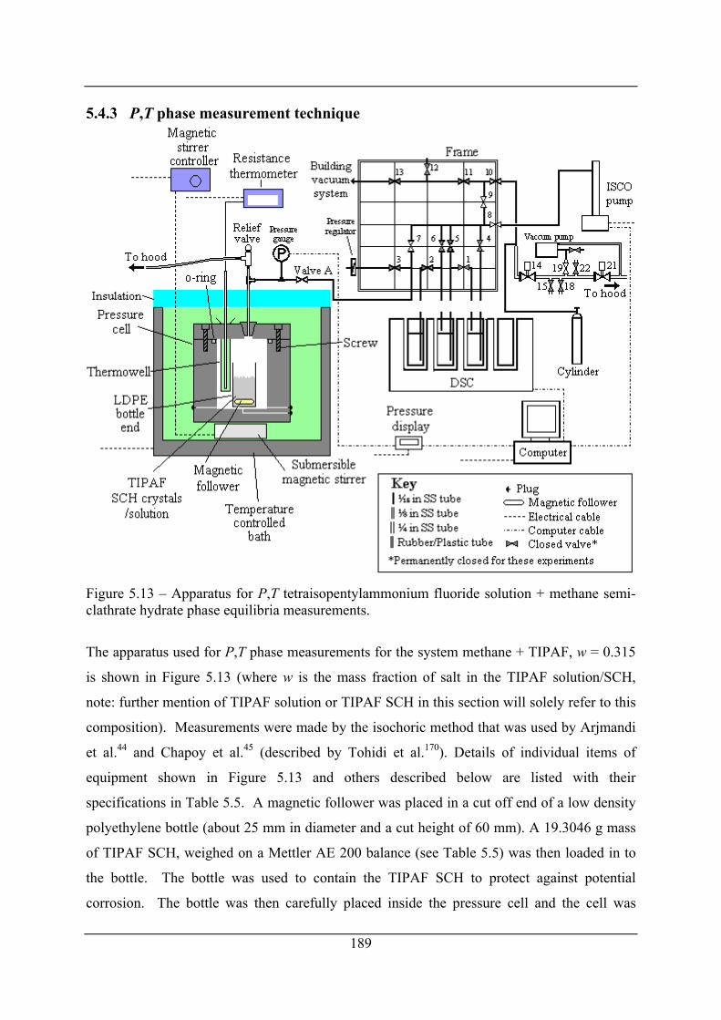
5.4.3 P,T phase measurement technique
Figure 5.13 – Apparatus for P,T tetraisopentylammonium fluoride solution + methane semi-clathrate hydrate phase equilibria measurements.
The apparatus used for P,T phase measurements for the system methane + TIPAF, w = 0.315
is shown in Figure 5.13 (where w is the mass fraction of salt in the TIPAF solution/SCH,
note: further mention of TIPAF solution or TIPAF SCH in this section will solely refer to this
composition). Measurements were made by the isochoric method that was used by Arjmandi
et al.44 and Chapoy et al.45 (described by Tohidi et al.170). Details of individual items of
equipment shown in Figure 5.13 and others described below are listed with their
specifications in Table 5.5. A magnetic follower was placed in a cut off end of a low density
polyethylene bottle (about 25 mm in diameter and a cut height of 60 mm). A 19.3046 g mass
of TIPAF SCH, weighed on a Mettler AE 200 balance (see Table 5.5) was then loaded in to
the bottle. The bottle was used to contain the TIPAF SCH to protect against potential
corrosion. The bottle was then carefully placed inside the pressure cell and the cell was
189
190
sealed by placement of an o-ring in the o-ring groove and by tightening the hexagon socket
head cap screws to the required torque using a torque wrench (Norbar 200). The cell was then
carefully placed in the temperature controlled bath (at 293.15 K) on top of a submersible
magnetic stirrer (note: the magnetic stirrer had been tested to ensure it worked with the
magnetic follower inside the cell before loading of the SCH and sealing of the cell). Methane
was purged in to the system to a pressure of about 0.5 MPa from the cylinder with valves (7 to
10 and A) open and valves (11 and 14) closed. The gas was then vented to the hood to close
to atmospheric pressure, by opening valve 14, valve 8 to the ISCO pump (model 260 D) was
then closed (the ISCO pump is not designed for pressures below atmospheric, note the ISCO
pump was empty (volume = 0.00 mL) for these steps) and valves (14 and 19) were then
opened and the vacuum pump was switched on (see Table 5.5) which reduced the pressure to
about 0.013 MPa. This process was repeated three times to purge air from the system. The
cell was then filled with methane to a pressure of about 1 MPa and the temperature controlled
bath was set to 313.15 K. By raising the temperature to 313.15 K all the SCH should have
dissociated. The system was then cooled back to 273.15 K and the gas was vented to the
hood to just above atmospheric pressure, followed by vacuuming using the vacuum pump
(valve 8 to the ISCO pump was again closed and valves (14 and 19) were opened with the
vacuum pump switched on). The purpose of this process was to remove potential air
(nitrogen or oxygen) molecules from the 512 cages of the SCH. The process was repeated
once more. The bath temperature was then set to 283.15 K. Methane was introduced in to the
ISCO pump from the cylinder with valves (8 to 10) open and valves (7 and A) closed. The
methane was introduced at a pressure of about 12.5 MPa and the ISCO pump was reversed to
a volume of about 200 ml. The cylinder valve was then closed and valves (7 and A) were
slowly opened to gradually let methane in to the cell. The cell was monitored for leaks by
checking for bubbles in the temperature controlled bath and by wetting connections with
Swagelok Snoop® liquid leak detection liquid. When the system pressure had stabilised to a
uniform value (about 8.5 MPa) the ISCO was set to pump at a constant flow rate of 10
mL/min until the pressure in the cell was about 20 MPa. At this point valves (7 to 10 and A)
were closed.
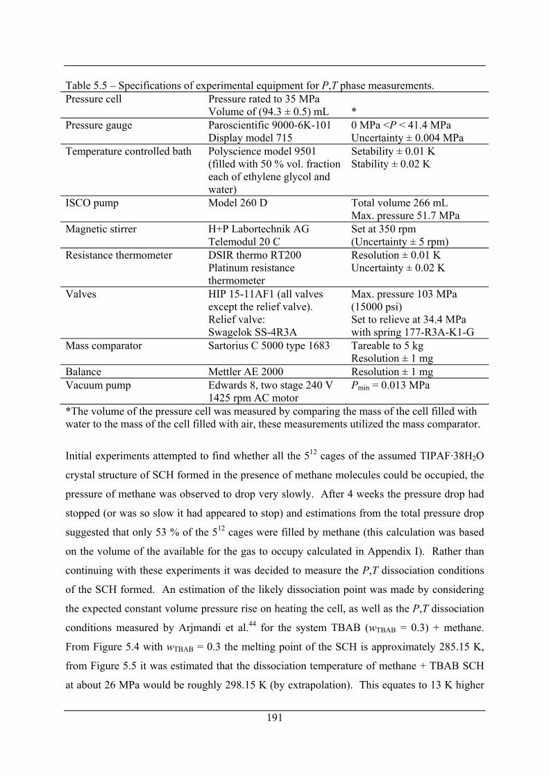
191
Table 5.5 – Specifications of experimental equipment for P,T phase measurements. Pressure cell Pressure rated to 35 MPa
Volume of (94.3 ± 0.5) mL *
Pressure gauge Paroscientific 9000-6K-101 Display model 715
0 MPa <P < 41.4 MPa Uncertainty ± 0.004 MPa
Temperature controlled bath Polyscience model 9501 (filled with 50 % vol. fraction each of ethylene glycol and water)
Setability ± 0.01 K Stability ± 0.02 K
ISCO pump Model 260 D Total volume 266 mL Max. pressure 51.7 MPa
Magnetic stirrer H+P Labortechnik AG Telemodul 20 C
Set at 350 rpm (Uncertainty ± 5 rpm)
Resistance thermometer DSIR thermo RT200 Platinum resistance thermometer
Resolution ± 0.01 K Uncertainty ± 0.02 K
Valves HIP 15-11AF1 (all valves except the relief valve). Relief valve: Swagelok SS-4R3A
Max. pressure 103 MPa (15000 psi) Set to relieve at 34.4 MPa with spring 177-R3A-K1-G
Mass comparator Sartorius C 5000 type 1683 Tareable to 5 kg Resolution ± 1 mg
Balance Mettler AE 2000 Resolution ± 1 mg Vacuum pump Edwards 8, two stage 240 V
1425 rpm AC motor Pmin = 0.013 MPa
*The volume of the pressure cell was measured by comparing the mass of the cell filled with water to the mass of the cell filled with air, these measurements utilized the mass comparator.
Initial experiments attempted to find whether all the 512 cages of the assumed TIPAF·38H2O
crystal structure of SCH formed in the presence of methane molecules could be occupied, the
pressure of methane was observed to drop very slowly. After 4 weeks the pressure drop had
stopped (or was so slow it had appeared to stop) and estimations from the total pressure drop
suggested that only 53 % of the 512 cages were filled by methane (this calculation was based
on the volume of the available for the gas to occupy calculated in Appendix I). Rather than
continuing with these experiments it was decided to measure the P,T dissociation conditions
of the SCH formed. An estimation of the likely dissociation point was made by considering
the expected constant volume pressure rise on heating the cell, as well as the P,T dissociation
conditions measured by Arjmandi et al.44 for the system TBAB (wTBAB = 0.3) + methane.
From Figure 5.4 with wTBAB = 0.3 the melting point of the SCH is approximately 285.15 K,
from Figure 5.5 it was estimated that the dissociation temperature of methane + TBAB SCH
at about 26 MPa would be roughly 298.15 K (by extrapolation). This equates to 13 K higher
192
than the melting point of the SCH under atmospheric conditions. It might be expected that
TIPAF SCH would be stable to a similar degree over the melting point of the SCH under
atmospheric conditions than TBAB SCH at the same pressure, therefore from the melting
point of TIPAF·38H2O of 305.6 K (using the value of Lipkowski et al.67, see Table 1.2) it was
estimated that the dissociation point at approximately 26 MPa would be roughly 317 K.
However as this was only a rough estimate, temperature steps began at 309.15 K. The
temperature was raised initially in steps of (1 to 2) K at a time. Approximately (20 to 28) h
was allowed for the system to come to equilibrium after each temperature step, by this time
the pressure (which was logged by computer, see Figure 5.13) had reached a new stable value.
Smaller temperature steps of between (0.1 and 0.5) K were taken when there was a steeper
rise in pressure between temperature steps indicating the start of dissociation of the SCH.
After the initial measurement was made the pressure was reduced in the cell by opening
valves (7, 8 and A) and reversing the ISCO pump slowly until the desired pressure was
achieved. The SCH was formed again by lowering the temperature of the bath to between
(273 and 283) K and then reheating the SCH to a temperature of 309 K just greater than the
melting point of the most stable SCH (TIPAF·27H2O, MP 307.8 K 67). The cycle of
temperature was repeated several times and increased the rate of pressure drop and hence
formation rate of methane enclathrated SCH. By heating to a temperature greater than that of
the atmospheric melting point of the most stable SCH under atmospheric conditions it was
figured that SCH structures that may not be able to enclathrate methane would also be
removed. These steps were repeated for each new measurement.
5.5 Results and discussion
5.5.1 Dissociation point measurements Figure 5.14 shows an example series of equilibrium point measurements for the TIPAF w =
0.315 solution/SCH + methane system for one dissociation point determination (note: all
reference to TIPAF solution/SCH referred to in this section refers to that with a mass fraction
of salt of w = 0.315 unless otherwise noted). Linear extrapolations were made from the points
before and after complete dissociation and the SCH + Aq + V point (labelled in the Figure
5.14) that was found at the intersection point of these linear lines.
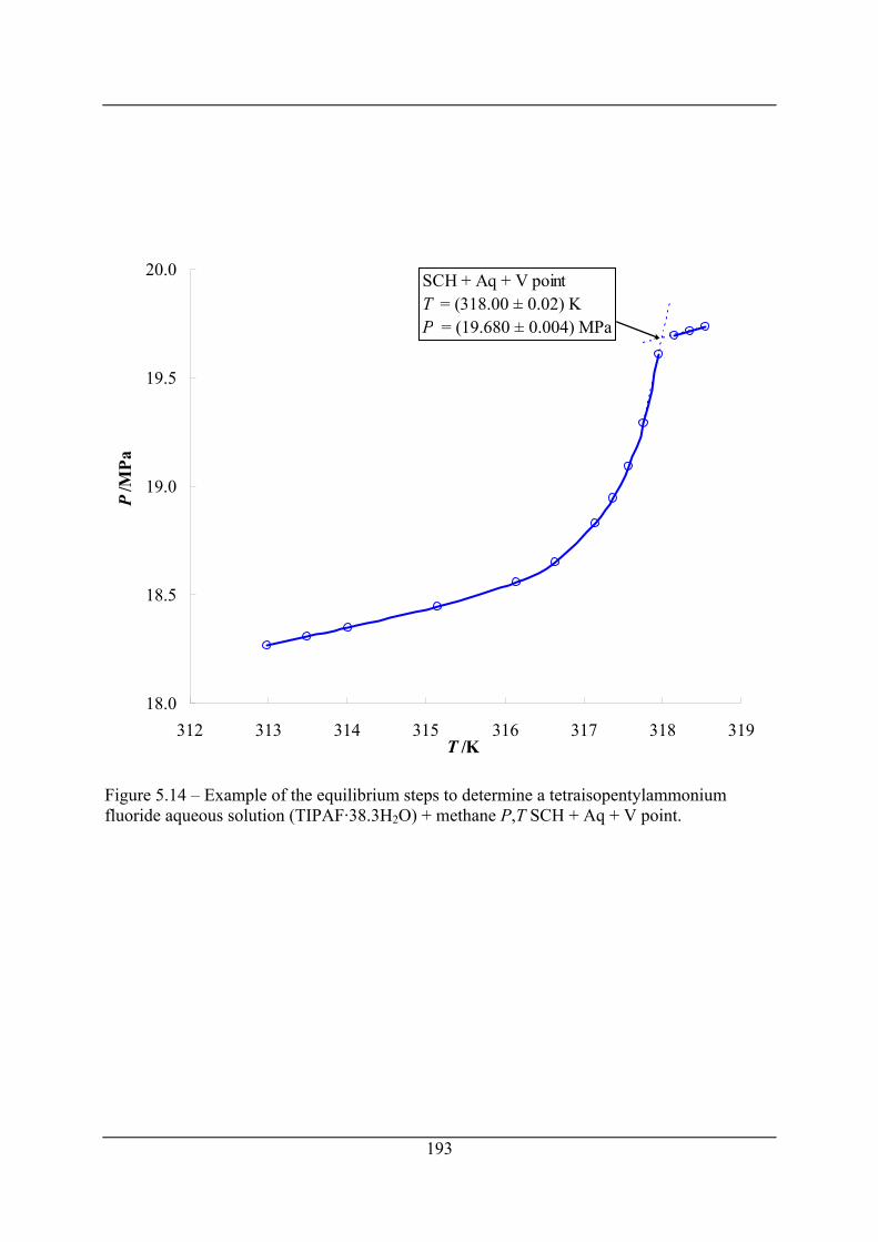
18.0
18.5
19.0
19.5
20.0
312 313 314 315 316 317 318 319T /K
P/M
Pa
SCH + Aq + V pointT = (318.00 ± 0.02) KP = (19.680 ± 0.004) MPa
Figure 5.14 – Example of the equilibrium steps to determine a tetraisopentylammonium fluoride aqueous solution (TIPAF·38.3H2O) + methane P,T SCH + Aq + V point.
193
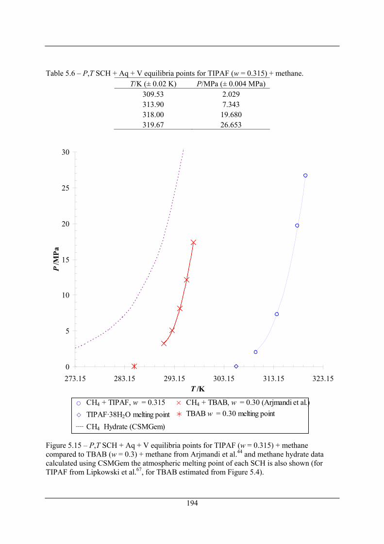
Table 5.6 – P,T SCH + Aq + V equilibria points for TIPAF (w = 0.315) + methane. T/K (± 0.02 K) P/MPa (± 0.004 MPa)
309.53 2.029 313.90 7.343 318.00 19.680 319.67 26.653
0
5
10
15
20
25
30
273.15 283.15 293.15 303.15 313.15 323.15T /K
P/M
Pa
CH4 + TIPAF, w = 0.315TIPAF·38H2O melting point CH4 Hydrate (CSMGem)----
CH4 + TBAB, w = 0.30 (Arjmandi et al.)TBAB w = 0.30 melting point
Figure 5.15 – P,T SCH + Aq + V equilibria points for TIPAF (w = 0.315) + methane compared to TBAB (w = 0.3) + methane from Arjmandi et al.44 and methane hydrate data calculated using CSMGem the atmospheric melting point of each SCH is also shown (for TIPAF from Lipkowski et al.67, for TBAB estimated from Figure 5.4).
194
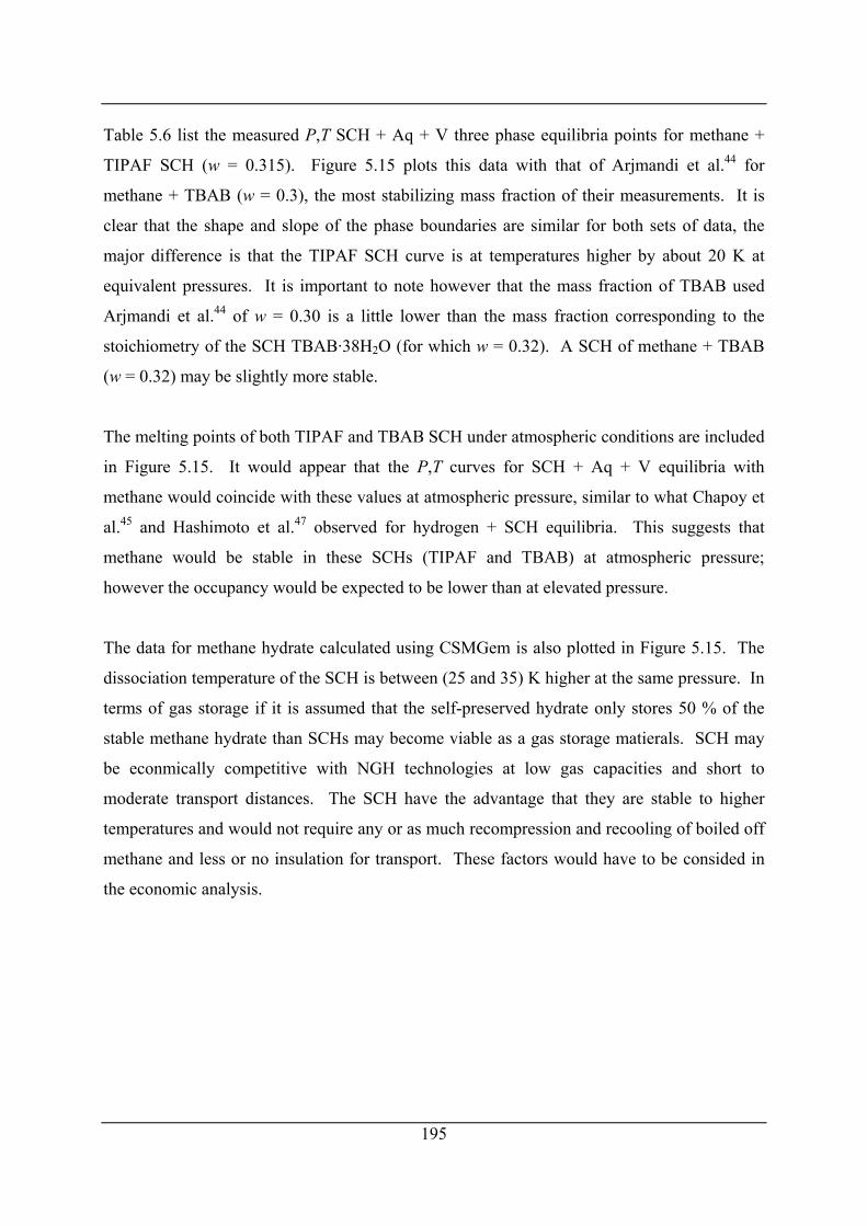
195
Table 5.6 list the measured P,T SCH + Aq + V three phase equilibria points for methane +
TIPAF SCH (w = 0.315). Figure 5.15 plots this data with that of Arjmandi et al.44 for
methane + TBAB (w = 0.3), the most stabilizing mass fraction of their measurements. It is
clear that the shape and slope of the phase boundaries are similar for both sets of data, the
major difference is that the TIPAF SCH curve is at temperatures higher by about 20 K at
equivalent pressures. It is important to note however that the mass fraction of TBAB used
Arjmandi et al.44 of w = 0.30 is a little lower than the mass fraction corresponding to the
stoichiometry of the SCH TBAB·38H2O (for which w = 0.32). A SCH of methane + TBAB
(w = 0.32) may be slightly more stable.
The melting points of both TIPAF and TBAB SCH under atmospheric conditions are included
in Figure 5.15. It would appear that the P,T curves for SCH + Aq + V equilibria with
methane would coincide with these values at atmospheric pressure, similar to what Chapoy et
al.45 and Hashimoto et al.47 observed for hydrogen + SCH equilibria. This suggests that
methane would be stable in these SCHs (TIPAF and TBAB) at atmospheric pressure;
however the occupancy would be expected to be lower than at elevated pressure.
The data for methane hydrate calculated using CSMGem is also plotted in Figure 5.15. The
dissociation temperature of the SCH is between (25 and 35) K higher at the same pressure. In
terms of gas storage if it is assumed that the self-preserved hydrate only stores 50 % of the
stable methane hydrate than SCHs may become viable as a gas storage matierals. SCH may
be econmically competitive with NGH technologies at low gas capacities and short to
moderate transport distances. The SCH have the advantage that they are stable to higher
temperatures and would not require any or as much recompression and recooling of boiled off
methane and less or no insulation for transport. These factors would have to be consided in
the economic analysis.
196
Chapter 6 CONCLUSIONS AND RECOMMENDATIONS
6.1 Conclusions
6.1.1 Dissociation enthalpies and plug dissociation times of sI and sII gas hydrates prepared from methane + ethane mixtures
P,T hydrate phase diagrams prepared using CSMGem at a high gas to water mole ratio (Ng/Nw
= 100) for a gas mixture of mole fractions 98.8 % methane + 1.2 % ethane reveal a similar
diagram to that of a multi-component processed natural gas (PNG) mixture of Bollavaram.54
A sII hydrate formation region occurs at low pressures and a sI region at high pressures
separated by a sI+sII+V boundary line/region exhibiting a negative dP/dT slope. This
indicates that a 98.8 % methane + 1.2 % ethane mixture can be representative of a PNG. A
phase diagram prepared for a mixture of mole fractions 65.4 % methane + 34.6 % ethane on
the other hand shows quite opposite behaviour with a sI region at lower pressures and a sII
region at higher pressure separated by sI+sII+V boundary line/region exhibiting a positive
dP/dT slope. This mixture was deemed to be non-representative of a PNG.
A further observation from the P,T hydrate phase diagrams was that a lnP versus 1/T plot of
the phase data for the mixture of mole fractions 98.8 % methane + 1.2 % ethane under sI
forming conditions aligned very closely with data plotted for pure methane hydrate. This
suggests from the Clapeyron equation that the dissociation enthalpies of sI hydrate of this
mixture would be almost identical to that of a pure methane sI hydrate.
Preferential enclathration was defined as the hydrate phase’s preference to enclathrate a
component or components of the gas thus stripping the gas phase of these components. An
interesting phenomena observed from P,T phase calculations of methane + ethane mixtures
was the existence of points were the water free composition of the hydrate is the same as that
of the free gas. At these point there was no preferential enclathration or stripping of the gas
phase. It was found however that these points where unstable, if a slight deviation in the
composition of the mixture occurs preferential enclathration and stripping would result. An
example of this was illustrated for a mixture of mole fractions 70 % methane + 30 % ethane at
15.77 MPa and 273.15 K. Predictions showed that if the feed gas was perturbed to a lower
197
mole fraction of methane the hydrate would preferentially enclathrate methane and the gas
phase methane mole fraction would drop. On the other hand if the feed gas was perturbed to a
higher mole fraction of methane the hydrate would preferentially enclathrate ethane and hence
the gas phase methane mole fraction would increase. These points however could still be
useful as the preferential enclathration is minimal and they could be used to form hydrates
under conditions where the water to gas mole ratio is higher, i.e. typical laboratory conditions
with minimal preferential enclathration or free gas stripping.
Structure I and structure II hydrate plugs were prepared from a mixture of mole fractions
65.4 % methane + 34.6 % ethane. The results showed that the dissociation time for the sII
hydrate plug of this mixture was shorter than that of the sI hydrate plug. This was the
opposite to the prediction made by the Peters’ CSMPlug model49 that the plug dissociation
time of a sII plug would be 30 % longer than that of a sI plug. Estimates of the enthalpies of
dissociation for each of these hydrates reveal that the dissociation enthalpy of sI hydrate is
predicted to be higher than that of the sII hydrate which explains the poor prediction since the
model assumes the enthalpy of dissociation of sII is greater than sI. The predicted enthalpies
of dissociation for sI and sII hydrates prepared from a mixture of mole fractions of 98.8 %
methane + 1.2 % ethane show the opposite, that the sII enthalpy of dissociation is higher than
that of the sI hydrate. Plugs were prepared of sI hydrates from a mixture of mole fraction
98.8 % methane + 1.2 % ethane and sII hydrates from a mixture of mole fraction 80 %
methane + 20 % ethane. Dissociation time measurements showed that on average the
dissociation time for the sII hydrate plug was 25 % longer than for a sI hydrate plug. This
agreed with the CSMPlug model prediction, probably as a result of the fact that the enthalpy
of dissociation of the sII hydrate was greater than the sI hydrate, like the model assumes. An
alternative hydrate dissociation model of Nguyen-Hong et al.51 was shown to predict that the
relative dissociation time of hydrate plugs of the same size, porosity and dissociation
conditions was approximately equal to the ratio of the dissociation enthalpy multiplied by the
hydrate density of each plug. This model and the experimental results both show that the
dissociation enthalpy is probably the most important factor in the determination of the plug
dissociation time.
198
Measurements of the dissociation enthalpy of sII hydrates with a mixture of mole fractions
98.8 % methane + 1.2 % ethane have been performed using a high pressure DSC at about
7 MPa. Two methods of formation were used, the first method involved forming the hydrate
within the DSC’s cell and second method involved cryogenically transferring hydrate formed
in a pressure cell. The overall conversion of water to hydrate was 64.26 % and 98.16 % for
these two methods respectively, and the enthalpies were (66.47 ± 0.50) kJ·mol-1 at 7.03 MPa
and (63.15 ± 0.50) kJ·mol-1 at 6.92 MPa. Generally higher conversion are viewed to give
better results,143 this is one reason why these two differ to a greater extent then the
uncertainty. Another possible reason is due to slightly different hydrate phase composition
because of the different formation methods. The measured values were also compared to
predictions provided from the Clapeyron equation using P,T phase data calculated in
CSMGem. It was assumed in these calculations that the gases were not soluble in water and
there was insignificant vaporisation of water into the vapour phase (however the volume of
each phase was taken in account by use of eq (3.17) for the compressibility factor difference).
Enthalpies of dissociation were calculated for sI and sII hydrate of the mixture of mole
fractions 65.4 % methane + 34.6 % ethane, as well as sII hydrates of the mixture of mole
fractions 98.8 % methane + 1.2 % ethane and sI pure methane hydrate. The measurement of
the enthalpy of dissociation of (63.15 ± 0.50) kJ·mol-1 at 6.92 MPa for the sII hydrate of the
mixture of mole fractions 98.8 % methane + 1.2 % ethane was within the uncertainty of the
Clapeyron equation calculated enthalpy. The Clapeyron equation calculated enthalpies of
dissociation for methane hydrate also compared within their uncertainty to published
calorimetric measurements. These results indicate that the Clapeyron equation enthalpies of
dissociation using the assumptions stated provides a good estimate of the true enthalpy.
Sloan and Fleyfel154,155 suggested that enthalpy of dissociation varies as a function of the size
of the guest for single guest hydrates. A comparison of the average guest diameter of each
cage for both the sI and sII hydrates of the mixture of mole fractions 65.4 % methane +
34.6 % ethane reveal that for the sI hydrate the large cage guest diameter does not change
much with pressure, however the guest average diameter for the small cages increases by
about 1.4 Å in 10 MPa. For the sII hydrate the large cage average guest size remains almost
constant with pressure and the small cage average guest size only increases by about 0.5 Å in
135 MPa. Comparing these results to the enthalpies of dissociation it clear to see that the sI
199
enthalpies for this mixture increases steeply with pressure, whereas the sII enthalpies remains
approximately constantly over a wide pressure range. This indicates that Sloan and Fleyfel’s
suggestion is correct and can be applied to hydrates of mixed guests. This has implications on
the plug dissociation time.
6.1.2 The modelling of preferential enclathration In doing the plug dissociation studies in this work at high methane mole fractions a
discontinuity was observed in the gas evolution rate and X-ray diffraction data indicated the
possibility of the presence of both sI and sII hydrate structures in some plugs. Models were
conceived for laboratory hydrate formations where there is typically a large mole ratio of gas
to water during hydrate formation. Two stepwise models of hydrate formation were presented
in Chapter 4 for the calculation of preferential enclathration of certain components in the
hydrate phase and associated stripping of these components from the vapour phase. The first
model was a constant pressure model whereby a gas is initially charged to a system containing
a piston or syringe pump and a cell filled with ice or water. As hydrate formation proceeds
the piston or syringe pump compresses the remaining gas to maintain constant pressure. This
model takes small steps in conversion of ice to hydrate and uses equilibrium CSMGem
predictions for the hydrate phase composition. The second model was a constant volume
system where a cell containing ice or water was charged with gas at an initial pressure and the
pressure was allowed to drop as hydrate formation proceeded. This model takes small steps
in the pressure drop and again uses equilibrium CSMGem predictions for the hydrate phase
composition.
A slightly modified constant pressure model was tested against experiments where the gas
composition was monitored by gas chromatography (GC) as hydrate formation proceeded. A
known amount of powdered ice was loaded into a pressure cell, the cell was pressurised with
a mixture of mole fractions 89.7 % methane + 10.3 % ethane. The cell was then heated above
the ice point to initiate hydrate formation and a syringe pump was used to maintain a constant
pressure as hydrate formation proceeded. Before samples were removed for GC
measurements the system was cooled to 258 K and mixing was achieved by cycling the
syringe pump up and down in pressure. One of the model’s assumptions was that there was
no direct conversion of ice to hydrate. This was observed to be true as during a period where
200
the cell was held at 258 K for over 6 days there was negligible change in the volume of gas
contained in the syringe pump at constant pressure. The GC measurements and the model
predictions of the free gas methane mole fraction were plotted as a function of pumped gas
volume (note the model had been modified to take in to account the removal of samples). The
plot showed the model exhibited similar trends to the experimental measurements, in that the
mole fraction of methane in the free gas increased with the volume of gas pumped. The
percentage deviation of the final methane mole fraction was +1.9 %, (92.5 % from GC and
94.3 % from the model). The total gas pumped experimentally was 183.68 mL, whereas the
model predicted a slightly lower 183.12 mL. From these results it was concluded that the
model is validated. The model-experiment discrepancy was likely due to the use of
equilibrium predictions of the hydrate phase composition. The phenomenological explanation
of the discrepancy was that methane can diffuse more quickly thorough a layer of hydrate
than ethane due to its smaller size. It was concluded therefore that it might be expected that
the hydrate would form with a higher mole fraction of methane than predicted by equilibrium
thermodynamics. As the constant volume model was similar in its assumptions and equations
it was assumed to also be validated by these results. These results prove it is possible to form
a hydrate plug containing both sI and sII hydrates if the typical laboratory formation
conditions of a large initial mole ratio of ice or water to gas is used in experiments due to
preferential enclathration and the accompanying stripping of components from the gas phase.
The formation of both sI and sII hydrates is more likely to occur if the initial gas composition
is close to a sI-sII boundary. In the experiments in this work the initial feed gas composition
did not have a high enough methane mole fraction to result in the formation of both sI and sII
hydrates.
6.1.3 Tetraisopentylammonium fluoride semi-clathrate hydrate (SCH) + methane P,T phase equilibria
Measurements of P,T SCH + Aq + V three phase equilibria points for methane +
tetraisopentylammonium fluoride (TIPAF) in aqueous solution (w = 0.315) were made
between temperatures of (309.53 and 319.67) K and between pressures of (2.029 and
26.653) MPa. The salt mass fraction was fixed by crystallisation of the SCH of structural
hydration number 38 that was measured by Karl Fischer titration to be 38.3. This SCH was
chosen as it has a melting point exceeding 30 °C as well as a relatively high number of cages
201
that could be filled by gas molecules. The phase boundary measured was similar in shape to
one measured by Arjmandi et al.44 for methane + tetrabutylammonium bromide (TBAB) in
aqueous solution (w = 0.30) except that it was approximately 20 K higher in temperature. The
results were also compared to the data of pure methane hydrate predicted using CSMGem.
The phase boundary for methane + TIPAF solution (w = 0.315) was between (25 and 35) K
higher at the same pressures. Comparison of the mass fraction of methane that could be
stored in a self-preserved methane hydrate at 267 K after a month with the estimated
maximum mass fraction of methane that could be stored in SCH indicate that SCH may be a
useful gas storage material. The SCH may be useful for similar applications for which NGH
technology has been shown to be economic, that is for lower gas field capacities and short to
moderate transport distances. The advantage is no or little refrigeration and less or no
insulation would be required for the storage of methane in this SCH.
6.2 Recommendations and future work It is clear from a review of the calorimetric enthalpies of dissociation of natural gas hydrate
constituents and mixtures that there is a general lack of data. Measurements of the enthalpies
of dissociation of hydrates of CO2, H2S or another highly water soluble gaseous guest would
be particularly useful for investigating assumptions associated with the use of the Clapeyron
equation (such results for CO2 hydrate may also prove useful for research on the sequestration
of CO2 in gas hydrates). Further measurement of the enthalpies of dissociation of hydrates
with mixed guest would also be useful to further test the validity of the Clapeyron equation.
(Note: more measurements might have been undertaken in this work had the DSC used been
more reliable).
Modifications might be made to the CSMPlug program. It might be useful to include an
option whereby the user may input an enthalpy of dissociation for their hydrate. Clapeyron
equation predictions of the enthalpy of dissociation might also be added to the code of
CSMGem. This would allow better predictions of the hydrate dissociation times.
For laboratory hydrate plug formation from gas mixtures that may either form sI or sII
hydrates it is recommended that models such as those presented in Chapter 4 of this work be
used to predict whether it is likely that more than one hydrate structure will form given an
202
initial amount of ice and gas. The use of the model may prevent unwanted mixtures of sI and
sII hydrate being formed. It is recommended though that all phases be characterised as much
as possible, preferably by structural analysis using X-ray diffraction, Raman spectroscopy or
NMR on samples of hydrate, to confirm its structure. It is also useful to know the final
composition of the gas used to form the hydrate plug as this may give an indication to
whether it is likely that more than one structure of hydrate has formed. This can be easily
measured by gas chromatography. The structural analysis of the hydrate may also reveal the
composition of the hydrate phase. This can also be measured by gas chromatography and a
comparison might prove useful and is not too difficult if hydrates samples are also required
for structural analysis.
A method to prevent changes in the gas composition during laboratory hydrate formations
from melting ice particles was proposed. This method relies upon the use of two gas
mixtures. One mixture would be used to initially pressurise a cell containing the ice particles;
this mixture might be at the composition of a typical pipeline natural gas. Once the initial
pressurization is completed the supply would be switched to a gas mixture of the expected
hydrate composition (on a water free basis) that would form from the initial gas mixture at a
high mole ratio of gas to water. This “formation gas” supply would be regulated in to the cell
at the pressure of the initial pressurisation. Thus as hydrate formation proceeds the initial gas
composition is replaced by the “formation gas” in order to maintain the initial gas
composition. This method is unproven and should be tested. The need for good mixing and
accurate knowledge of the hydrate phase water free composition would probably be
important.
There are only limited published measurements of phase equilibria of semi-clathrate hydrates
(SCH) and gases. Most measurements so far have focussed on hydrogen semi-clathrates. The
highest possible mass fraction of hydrogen able to be stored however is 0.83 % for the
tributylphosphine oxide (TBPO) SCH TBPO·34.5H2O assuming single occupancy of
hydrogen in the 512 cages. For the same assumption TIPAF·38H2O SCH can only store
0.6 %. These low values are unlikely to be of commercial interest for gas storage purposes.
The storage of gases such as methane may have more commercial applications. If SCHs such
as that of tributylphosphine oxide can store as much methane as self preserved sI methane
203
hydrate it might be useful for the transportation of methane under similar conditions for which
NGH has shown to be economic means of methane transportation. The economics of
methane storage and transportation in SCHs under these conditions of low gas field capacity
and short to moderate transport distance should be investigated. Given that some SCH are
stable to greater than 30 °C they may require no or less refrigeration and insulation. The
current method of transporting methane (or natural gas containing mostly methane) large
distances is in the form of liquid as liquefied natural gas (LNG tankers). These tankers must
be refrigerated as the boiling point of methane is only about 112 K (from NIST Refprop168).
The extra mass of refrigeration systems, insulation and LNG plant should be assessed when
making comparison of the storage capacities. A study could be made of these considerations
to see if it would make sense to consider SCHs as methane storage materials at higher field
capacities that are currently economic only for methane transportation by LNG.
The research of Shimada et al.63 and Kamata et al.64,195 have shown that it is possible to
separate gas mixtures by the formation of SCH. Further research on gas separation using
SCH should be considered. One possible SCH that could be studied is TIPAF·27H2O; it
contains the 5444 cage that only very small molecules such as hydrogen or helium could
potentially fill (see Appendix B for a size estimate of this cage). The exclusion of large
molecules by this SCH might be useful for purification of hydrogen.
204
REFERENCES (1) Sloan, E. D. Clathrate Hydrates of Natural Gases. 2nd ed. ed.; Chemical Industries;
Marcel Dekker: New York, 1998; Vol. 73, pp 705.
(2) Sloan, E. D.; Koh, C. A. Clathrate Hydrates of Natural Gases. 3rd ed.; Chemical
Industries; Taylor & Francis CRC press: Boca Raton, FL, 2007.
(3) Dyadin, Y. A.; Udachin, K. A. Clathrate Polyhydrates of Peralkylonium Salts and Their
Analogs. J. Struct. Chem. 1987, 28, 394-432
(4) Jeffrey, G. A. Hydrate Inclusion Compounds. In Inclusion Compounds, Atwood, J. L.;
Davies, J. E. D.; MacNicol, D. D., Eds.; 1984; Vol. 1, pp 135-190.
(5) Feil, D.; Jeffrey, G. A. Polyhedral Clathrate Hydrates .II. Structure of Hydrate of Tetra
Iso-Amyl Ammonium Fluoride. J. Chem. Phys. 1961, 35, 1863-1873.
(6) Nakayama, H.; Watanabe, K. Hydrates of Organic Compounds. II. The Effect of Alkyl
Groups on the Formation of Quaternary Ammonium Fluoride Hydrates. Bull. Chem. Soc.
Jpn. 1976, 49, 1254-6.
(7) Aladko, L. S.; Dyadin, Y. A.; Rodionova, T. V.; Terekhova, I. S. Clathrate Hydrates of
Tetrabutylammonium and Tetraisoamylammonium Halides. J. Struct. Chem. 2002, 43,
990-994.
(8) Aladko, L. S.; Dyadin, Y. A.; Rodionova, T. V.; Terekhova, I. S. Effect of Size and
Shape of Cations and Anions on Clathrate Formation in the System: Halogenides of
Quaternary Ammonium Bases and Water. J. Mol. Liq. 2003, 106, 229-238.
(9) Priestly, J. Experiments and Observations of Different Kinds of Air and Other Branches
of Natural Philosophy, Connected with the Subject. In Observations on the Freezing of
Water, impregnated with Fluor Acid Air, and with Vitriolic Acid Air, Thomas Pearson:
Birmingham, 1790; Vol. 2, pp 359-363.
(10) Prieto-Ballesteros, O.; Kargel, J. S.; Fernandez-Sampedro, M.; Selsis, F.; Martinez, E. S.;
Hogenboom, D. L. Evaluation of the possible presence of clathrate hydrates in Europa's
icy shell or seafloor. Icarus 2005, 177, 491-505.
(11) Davidson, D. W. Clathrate Hydrates. In Water in Crystalline Hydrates; Aqueous
Solutions of Simple Nonelectrolytes, Franks, F., Ed. Water: A Comprehensive Treatise,
Plenum: New York, 1973; Vol. 2, pp 115-234.
205
(12) Davy, H. The Bakerian Lecture. On some of the Combinations of Oxymuriatic gas and
Oxygene, and on the chemical Relations of these Principles, to inflammable Bodies.
Philos. Trans. R. Soc. London 1811, 101, 1-35.
(13) Faraday, M. On Fluid Chlorine. Philos. Trans. R. Soc. London 1823, 113, 160-165.
(14) Stuart, H. A.; Klemm, W.; Schmitz-Dumont, O.; von Stackelberg, M.; Nowotny, H.
Structure of Inorganic Substances. FIAT Rev. German Sci. 1939-46, Inorg. Chem., Pt. IV
1948, 1-109.
(15) von Stackelberg, M.; Gotzen, O.; Pietuchovsky, J.; Witscher, O.; Frühbuss, H.; Meinhold,
W. Structure and Formula of Gas Hydrates. Fortschritte der Mineralogie 1947, 26, 122-
124.
(16) von Stackelberg, M. Solid Gas Hydrates. Naturwissenschaften 1949, 36, 327-33,359-62.
(17) Claussen, W. F. Suggested Structures of Water in Inert Gas Hydrates. J. Chem. Phys.
1951, 19, 259-260.
(18) Claussen, W. F. Erratum: Suggested Structures of Water in Inert Gas Hydrates. J. Chem.
Phys. 1951, 19, 662.
(19) von Stackelberg, M.; Müller, H. R. The Structure of Gas Hydrates. Naturwissenschaften
1951, 38, 456.
(20) von Stackelberg, M.; Müller, H. R. On the Structure of Gas Hydrates. J. Chem. Phys.
1951, 19, 1319-1320.
(21) Claussen, W. F. A 2nd Water Structure for Inert Gas Hydrates. J. Chem. Phys. 1951, 19,
1425-1426.
(22) Müller, H. R.; von Stackelberg, M. Structure of Gas Hydrates. Naturwissenschaften 1952,
39, 20-1.
(23) Pauling, L.; Marsh, R. E. The Structure of Chlorine Hydrate. Proc. Natl. Acad. Sci. U. S.
A. 1952, 38, 112-118.
(24) McMullan, R. K.; Jeffrey, G. A. Polyhedral Clathrate Hydrates .IX. Structure of Ethylene
Oxide Hydrate. J. Chem. Phys. 1965, 42, 2725-2732.
(25) Mak, T. C. W.; McMullan, R. K. Polyhedral Clathrate Hydrates .X. Structure of Double
Hydrate of Tetrahydrofuran and Hydrogen Sulfide. J. Chem. Phys. 1965, 42, 2732-2737.
(26) Kirchner, M. T.; Boese, R.; Billups, W. E.; Norman, L. R. Gas Hydrate Single-Crystal
Structure Analyses. J. Am. Chem. Soc. 2004, 126, 9407-9412.
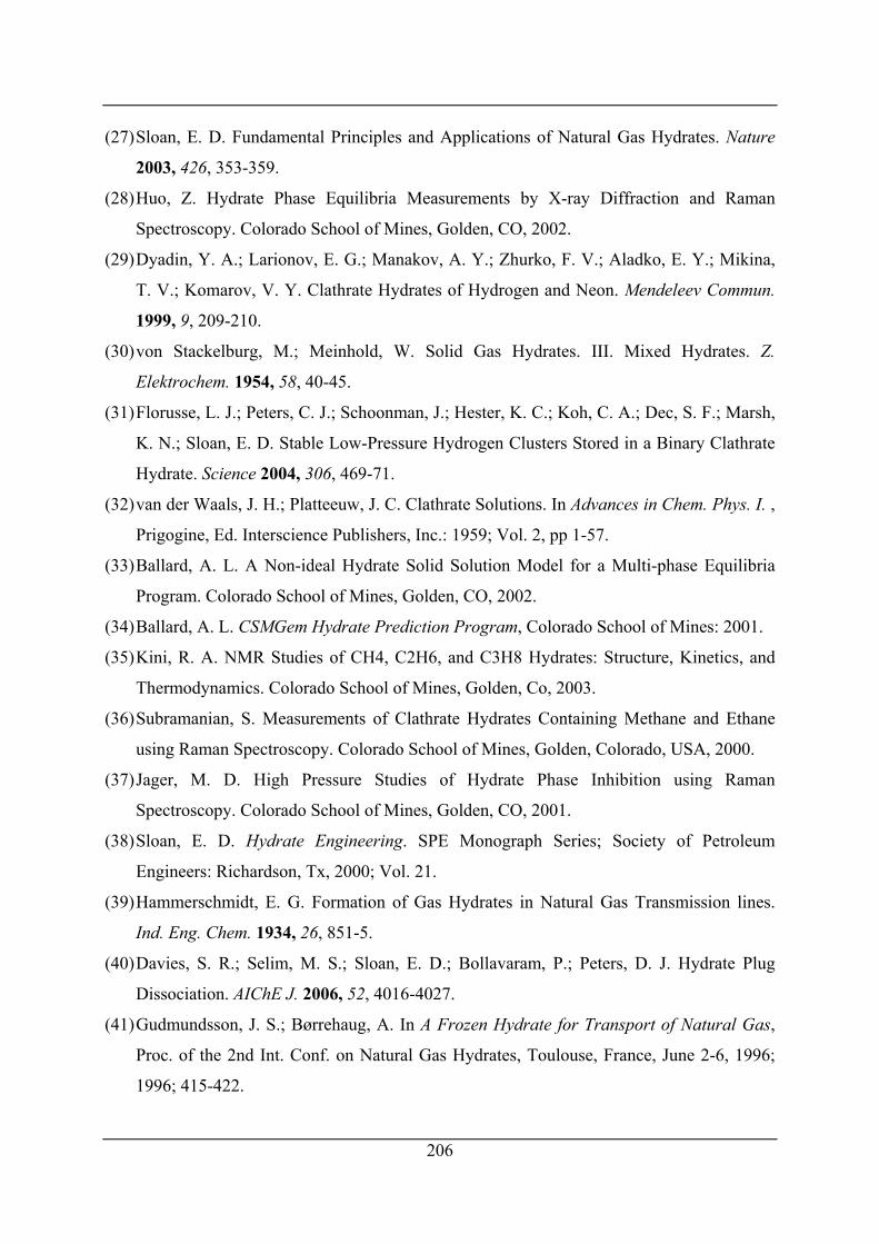
206
(27) Sloan, E. D. Fundamental Principles and Applications of Natural Gas Hydrates. Nature
2003, 426, 353-359.
(28) Huo, Z. Hydrate Phase Equilibria Measurements by X-ray Diffraction and Raman
Spectroscopy. Colorado School of Mines, Golden, CO, 2002.
(29) Dyadin, Y. A.; Larionov, E. G.; Manakov, A. Y.; Zhurko, F. V.; Aladko, E. Y.; Mikina,
T. V.; Komarov, V. Y. Clathrate Hydrates of Hydrogen and Neon. Mendeleev Commun.
1999, 9, 209-210.
(30) von Stackelburg, M.; Meinhold, W. Solid Gas Hydrates. III. Mixed Hydrates. Z.
Elektrochem. 1954, 58, 40-45.
(31) Florusse, L. J.; Peters, C. J.; Schoonman, J.; Hester, K. C.; Koh, C. A.; Dec, S. F.; Marsh,
K. N.; Sloan, E. D. Stable Low-Pressure Hydrogen Clusters Stored in a Binary Clathrate
Hydrate. Science 2004, 306, 469-71.
(32) van der Waals, J. H.; Platteeuw, J. C. Clathrate Solutions. In Advances in Chem. Phys. I. ,
Prigogine, Ed. Interscience Publishers, Inc.: 1959; Vol. 2, pp 1-57.
(33) Ballard, A. L. A Non-ideal Hydrate Solid Solution Model for a Multi-phase Equilibria
Program. Colorado School of Mines, Golden, CO, 2002.
(34) Ballard, A. L. CSMGem Hydrate Prediction Program, Colorado School of Mines: 2001.
(35) Kini, R. A. NMR Studies of CH4, C2H6, and C3H8 Hydrates: Structure, Kinetics, and
Thermodynamics. Colorado School of Mines, Golden, Co, 2003.
(36) Subramanian, S. Measurements of Clathrate Hydrates Containing Methane and Ethane
using Raman Spectroscopy. Colorado School of Mines, Golden, Colorado, USA, 2000.
(37) Jager, M. D. High Pressure Studies of Hydrate Phase Inhibition using Raman
Spectroscopy. Colorado School of Mines, Golden, CO, 2001.
(38) Sloan, E. D. Hydrate Engineering. SPE Monograph Series; Society of Petroleum
Engineers: Richardson, Tx, 2000; Vol. 21.
(39) Hammerschmidt, E. G. Formation of Gas Hydrates in Natural Gas Transmission lines.
Ind. Eng. Chem. 1934, 26, 851-5.
(40) Davies, S. R.; Selim, M. S.; Sloan, E. D.; Bollavaram, P.; Peters, D. J. Hydrate Plug
Dissociation. AIChE J. 2006, 52, 4016-4027.
(41) Gudmundsson, J. S.; Børrehaug, A. In A Frozen Hydrate for Transport of Natural Gas,
Proc. of the 2nd Int. Conf. on Natural Gas Hydrates, Toulouse, France, June 2-6, 1996;
1996; 415-422.
207
(42) Nakajima, Y.; Takaoki, T.; Ohgaki, K.; Ota, S. In Use of Hydrate Pellets for
Transportation of Natural Gas - II; Proposition of Natural Gas Transportation in Form
of Hydrate Pellets, Proc. of the 4th Int. Conf. on Gas Hydrates, Yokohama, Japan, May
19-23, 2002; 2002; 987-990.
(43) Shirota, H.; Aya, I.; Namie, S.; Bollavaram, P.; Turner, D. In Measurement of Methane
Hydrate Dissociation for Application to Natural Gas Storage and Transportation, Proc.
of the 4th Int. Conf. on Gas Hydrates, Yokohama, Japan, May 19-23, 2002; 2002.
(44) Arjmandi, M.; Chapoy, A.; Tohidi, B. Equilibrium Data of Hydrogen, Methane,
Nitrogen, Carbon Dioxide, and Natural Gas in Semi-Clathrate Hydrates of Tetrabutyl
Ammonium Bromide. J. Chem. Eng. Data 2007, 52, 2153-2158.
(45) Chapoy, A.; Anderson, R.; Tohidi, B. Low-Pressure Molecular Hydrogen Storage in
Semi-clathrate Hydrates of Quaternary Ammonium Compounds. J. Am. Chem. Soc. 2007,
129, 746-747.
(46) Hashimoto, S.; Murayama, S.; Sugahara, T.; Sato, H.; Ohgaki, K. Thermodynamic and
Raman spectroscopic studies on H2 + tetrahydrofuran + water and H2 + tetra-n-butyl
ammonium bromide + water mixtures containing gas hydrates. Chem. Eng. Sci. 2006, 61,
7884-7888.
(47) Hashimoto, S.; Sugahara, T.; Moritoki, M.; Sato, H.; Ohgaki, K. Thermodynamic
stability of hydrogen + tetra-n-butyl ammonium bromide mixed gas hydrate in
nonstoichiometric aqueous solutions. Chem. Eng. Sci. 2008, 63, 1092-1097.
(48) Park, Y.; Kim, D.-Y.; Lee, J.-W.; Huh, D.-G.; Park, K.-P.; Lee, J.; Lee, H. Sequestering
Carbon Dioxide into Complex Structures of Naturally Occurring Gas Hydrates. Proc.
Natl. Acad. Sci. U. S. A. 2006, 103, 12690-12694.
(49) Peters, D. J. A Study of Hydrate Dissociation in Pipelines by the Method of Two-Sided
Depressurisation: Experiment and Model. Colorado School of Mines, Golden, 1999.
(50) Gupta, A. Methane Hydrate Dissociation Measurements and Modeling: The Role of Heat
Transfer and Reaction Kinetics. Colorado School of Mines, Golden, CO, 2007.
(51) Nguyen-Hong, D.; Gruy, F.; Herri, J. M. Experimental Data and Approximate Estimation
for Dissociation Time of Hydrate Plugs. Chem. Eng. Sci. 2006, 61, 1846-1853.
(52) Moridis, G. J. In Numerical Studies of Gas Production From Methane Hydrates, Proc.
SPE Gas Technology Symposium, Calgary, Canada April 30 - May 2nd, 2002; 2002;
75691.
208
(53) Hong, H.; Pooladi-Darvish, M.; Bishnoi, P. R. Analytical Modelling of Gas Production
from Hydrates in Porous Media. J. Can. Pet. Technol. 2003, 42, 45-56.
(54) Bollavaram, P. Hydrate Plug Dissociation in Pipelines by Pressure Reduction:
Experiment and Modeling. Colorado School of Mines, Golden, Colorado, 2003.
(55) Fowler, D. L.; Loebenstein, D. B.; Pall; Kraus, C. A. Some Unusual Hydrates of
Quaternary Ammonium Salts. J. Am. Chem. Soc. 1940, 62, 1140-1142.
(56) Beurskens, G.; Jeffrey, G. A.; McMullan, R. K. Polyhedral Clathrate Hydrates .VI.
Lattice Type and Ion Distribution in Some New Peralkyl Ammonium, Phosphonium, and
Sulfonium Salt Hydrates. J. Chem. Phys. 1963, 39, 3311-3315.
(57) Jeffrey, G. A.; McMullan, R. K. Polyhedral Clathrate Hydrates .IV. Structure of Tri N-
Butyl Sulfonium Fluoride Hydrate. J. Chem. Phys. 1962, 37, 2231-2239.
(58) Alekseev, V. I.; Gatilov, Y. V.; Polyanskaya, T. M.; Bakakin, V. V.; Dyadin, Y. A.;
Gaponenko, L. A. Characteristic Features of the Production of the Hydrate Framework
Around the Hydrophobic-Hydrophillic Unit in the Crystal Structure of the Clathrate Tri-
n-butylphosphine Oxide 34.5-Hydrate. J. Struct. Chem. 1982, 23, 395-399.
(59) Bonamico, M.; McMullan, R. K.; Jeffrey, G. A. Polyhedral Clathrate Hydrates .III.
Structure of Tetra N-Butyl Ammonium Benzoate Hydrate. J. Chem. Phys. 1962, 37,
2219-2231.
(60) McMullan, R.; Jeffrey, G. A. Hydrates of the Tetra n-Butyl and Tetra i-Amyl Quaternary
Ammonium Salts. J. Chem. Phys. 1959, 31, 1231-1234.
(61) McMullan, R. K.; Jeffrey, G. A.; Bonamico, M. Polyhedral Clathrate Hydrates .V.
Structure of Tetra-N-Butyl Ammonium Fluoride Hydrate. J. Chem. Phys. 1963, 39, 3295-
3310.
(62) Shimada, W.; Shiro, M.; Kondo, H.; Takeya, S.; Oyama, H.; Ebinuma, T.; Narita, H.
Tetra-n-butylammonium Bromide-Water (1/38) Acta Crystallogr., Sect. C: Cryst. Struct.
Commun. 2005, 61, O65-O66
(63) Shimada, W.; Ebinuma, T.; Oyama, H.; Kamata, Y.; Takeya, S.; Uchida, T.; Nagao, J.;
Narita, H. Separation of Gas Molecule using Tetra-n-butyl Ammonium Bromide Semi-
Clathrate Hydrate Crystals. Jpn. J. Appl. Phys., Part 2 2003, 42, L129-L131.
(64) Kamata, Y.; Oyama, H.; Shimada, W.; Ebinuma, T.; Takeya, S.; Uchida, T.; Nagao, J.;
Narita, H. Gas Separation Method Using Tetra-n-butylammonium Bromide Semi-
Clathrate Hydrate. Jpn. J. Appl. Phys., Part 1 2004, 43, 362-365.
209
(65) Stupin, D. Y.; Stravitnaya, O. S. The Sorption of Sulphur Dioxide By the Clathrate
Hydrates of Tetrabutylammonium Bromide and Acetate. Russ. J. Phys. Chem. 1991, 65,
672-675.
(66) Stupin, D. Y.; Stravitnaya, O. S. The Sorption of Sulphur Dioxide By the Clathrates of
Tetrabutylammonium and Tetraisopentylammonium Phthalates. Russ. J. Phys. Chem.
1991, 65, 670-672.
(67) Lipkowski, J.; Suwinska, K.; Rodionova, T. V.; Udachin, K. A.; Dyadin, Y. A. Phase and
X-ray Study of Clathrate Formation in the Tetraisoamylammonium Fluoride-Water
System. J. Inclusion Phenom. 1994, 17, 137-48.
(68) Duc, N. H.; Chauvy, F.; Herri, J.-M. CO2 Capture By Hydrate Crystallization – A
Potential Solution For Gas Emission of Steelmaking Industry. Energy Convers. Manage.
2007, 48, 1313-1322.
(69) Oyama, H.; Shimada, W.; Ebinuma, T.; Kamata, Y.; Takeya, S.; Uchida, T.; Nagao, J.;
Narita, H. Phase diagram, latent heat, and specific heat of TBAB semiclathrate hydrate
crystals. Fluid Phase Equilib. 2005, 234, 131-135.
(70) ACD ChemSketch Freeware (Downloadable from www.acdlabs.com), Version 10.02;
Advanced Chemistry Development: Toronto, Canada, 2006.
(71) Subramanian, S.; Ballard, A. L.; Kini, R. A.; Dec, S. F.; Sloan, E. D. Structural
Transitions in Methane + Ethane Gas Hydrates. Part I: Upper Transition Point and
Applications. Chem. Eng. Sci. 2000, 55, 5763-5771.
(72) Subramanian, S.; Kini, R. A.; Dec, S. F.; Sloan, E. D., Jr. Evidence of Structure II
Hydrate Formation from Methane + Ethane Mixtures. Chem. Eng. Sci. 2000, 55, 1981-
1999.
(73) Marsh, K. N.; O'Hare, P. A. G., Eds., Solution Calorimetry. Experimental
thermodynamics; For IUPAC, Blackwell Scientific: Oxford, U.K., 1994; Vol. IV, p 576.
(74) Goodwin, A. R. H.; Marsh, K. N.; Wakeham, W. A. Measurement of the Thermodynamic
Properties of Single Phases. Experimental Thermodynamics; For IUPAC, Elsevier:
Amsterdam, 2003; Vol. VI.
(75) Claudy, P. M. Differential Scanning Calorimetry. In Measurement of the Thermodynamic
Properties of Single Phases, Goodwin, A. R. H.; Marsh, K. N.; Wakeham, W. A., Eds.;
Experimental thermodynamics, For IUPAC, Elsevier: Amsterdam, Netherlands, 2003;
Vol. VI, pp 348-368.
210
(76) Boersma, S. L. A Theory of Differential Thermal Analysis and New Methods of
Measurement and Interpretation. J. Am. Ceram. Soc. 1955, 38, 281-284.
(77) Mraw, S. C. Differential Scanning Calorimetry. In Specific heat of solids, Cezairliyan,
A.; Ho, C. Y.; Anderson, A. C., Eds.; CINDAS Data Series on Material Properties. Group
I, Theory, Estimation, and Measurement of Properties, Hemisphere: New York, 1988;
Vol. 1-2, pp 395-433.
(78) Marsh, K. N. Recommended Reference Materials for the Realization of Physicochemical
Properties. Blackwell Scientific Boston, MA, 1987.
(79) Multi-cell Differential Scanning Calorimeter User’s Manual. 3rd ed.; Calorimetry
Sciences Corporation: Lindon, UT, 1999.
(80) Nobelprize.org. The Nobel Prize in Physics 1901 Awarded to Wilhelm Roentgen "In
Recognition of the Extraordinary Services He Has Rendered by the Discovery of the
Remarkable Rays Subsequently Named after Him".
http://nobelprize.org/nobel_prizes/physics/laureates/1901/ (accessed 31-Oct-07)
(81) Nobelprize.org. The Nobel Prize in Physics 1914 Awarded to Max von Laue "For His
Discovery of the Diffraction of X-rays by Crystals".
http://nobelprize.org/nobel_prizes/physics/laureates/1914/ (accessed 31-Oct-07)
(82) Nobelprize.org. The Nobel Prize in Physics 1915 Awarded to William H Bragg and
William L Bragg "For Their Services in the Analysis of Crystal Structure by Means of X-
rays". http://nobelprize.org/nobel_prizes/physics/laureates/1915/ (accessed 31-Oct-07)
(83) Ladd, M. F. C.; Palmer, R. A. Structure Determination by X-ray Crystallography 4th ed.;
Kluwer Academic/Plenum: New York, 1993.
(84) Rietveld, H. M. A Profile Refinement Method for Nuclear and Magnetic Structures. J.
Appl. Crystallogr. 1969, 2, 65-71.
(85) Cambridge Structural Database. http://www.ccdc.cam.ac.uk/products/csd/ (accessed 29-
Oct-07); The Cambridge Crystallographic Data Centre
(86) Powder Diffraction File http://www.icdd.com/products/overview.htm (accessed 29-Oct-
07); International Centre for Diffraction Data
(87) Kraus, W.; Nolze, G. Powder Cell 2.4 for Windows (Downloadable from
ftp://ftp.bam.de/Powder_Cell/pcw23.exe), Bundesanstalt für Materialfoschung und -
prüfung: 2000.
(88) Owston, P. G. The Structure of Ice. Q. Rev. Chem. Soc. 1951, 5, 344-363.
211
(89) Jones, E. R.; Childers, R. L. Contemporary College Physics 2nd ed.; Addison-Wesley:
Readings, Massachusetts, 1993.
(90) Skoog, D. A.; Holler, F. J.; Nieman, T. A. Principles of Instrumental Analysis. 5th edn
ed.; Harcourt Brace College Publishers: Philadelphia, 1998.
(91) Nobelprize.org. The Nobel Prize in Physics 1930 Awarded to Venkata Raman "For His
Work on the Scattering of Light and for the Discovery of the Effect Named After Him".
http://nobelprize.org/nobel_prizes/physics/laureates/1901/ (accessed 31-Oct-07)
(92) Sum, A. K.; Burruss, R. C.; Sloan, E. D. Measurement of Clathrate Hydrates via Raman
Spectroscopy. J. Phys. Chem. B 1997, 101, 7371-7377.
(93) Subramanian, S.; Kini, R. A.; Dec, S. F.; Sloan, E. D. Structural Transition Studies in
Methane + Ethane Hydrates using Raman and NMR. Ann. N. Y. Acad. Sci. 2000, 912,
873-886.
(94) Subramanian, S.; Sloan, E. D. Trends in Vibrational Frequencies of Guests Trapped in
Clathrate Hydrate Cages J. Phys. Chem. B 2002, 106, 4348-4355.
(95) Martin, A. J. P.; Synge, R. L. M. A New Form of Chromatogram Employing Two Liquid
Phases. Biochem. J. 1941, 35, 1358-1368.
(96) James, A. T.; Martin, A. J. P. Gas-Liquid Partition Chromatography: The Separation and
Micro-Estimation of Volatile Fatty Acids from Formic Acid to Dodecanoic Acid
Biochem. J. 1952, 50, 679-690.
(97) Martin, A. J. P. The Development of Partition Chromatography, Nobel Lecture.
http://nobelprize.org/nobel_prizes/chemistry/laureates/1952/martin-lecture.pdf (accessed
23-Jan-08)
(98) Nobelprize.org. The Nobel Prize in Chemistry 1952 Awarded to Archer Martin and
Richard Synge "For Their Invention of Partition Chromatography".
http://nobelprize.org/nobel_prizes/chemistry/laureates/1952/ (accessed 31-Oct-07)
(99) Fischer, K. New Method for the Volumetric Determination of Water Contents in Liquids
and Solids. Angew. Chem. 1935, 48, 394-396.
(100) Wieland, G. Water Determination by Karl Fischer Titration. GIT VERLAG:
Beerfelden, Germany, 1987.
(101) McDowell, C. A.; Raghunathan, P. A Nuclear Magnetic Resonance Study of
Molecular Motion and "Guest" Structure in the Clathrate Hydrates of (i-C5H11)4NF and
(n-C4H9)4NF. Mol. Phys. 1968, 15, 259-270.
212
(102) Nobelprize.org. The Nobel Prize in Physics 1952 Awarded to Felix Bloch and Edward
Purcell "For Their Development of New Methods for Nuclear Magnetic Precision
Measurements and Discoveries in Connection Therewith".
http://nobelprize.org/nobel_prizes/physics/laureates/1952/ (accessed 28-Oct-07)
(103) Brown, W. H. Organic Chemistry. 1st ed.; Saunders College Publishing: Fort Worth,
TX, 1995.
(104) Harmon, K. M.; Bulgarella, J. A. Hydrogen Bonding Part 59. NMR Study of N,N,N-
Trimethyl-1-adamantylammonium, Trimethyl-i-pentylammonium, and Tetra-i-
pentylammonium Ions; an Explanation for the Anomalous Hydration Behavior of N,N,N-
Trimethyl-1-adamantylammonium Ion Salts. J. Mol. Struct. 1994, 326, 157-162.
(105) Sigma Aldrich Online Catalog, F-T NMR of Triethylamine.
http://www.sigmaaldrich.com/spectra/fnmr/FNMR003893.PDF (accessed 04-May-07)
(106) Sigma Aldrich Online Catalog, F-T NMR of Tripropylamine.
http://www.sigmaaldrich.com/spectra/fnmr/FNMR003898.PDF (accessed 04-May-07)
(107) Sigma Aldrich Online Catalog, F-T NMR of Trihexylamine.
http://www.sigmaaldrich.com/spectra/fnmr/FNMR002298.PDF (accessed 04-May-07)
(108) Heinsen, M. J.; Pochapsky, T. C. Site-Selective Deuterium Labeling of the
Tetrabutylammonium Cation. J. Labelled Compd. Radiopharm. 2000, 43, 473-480.
(109) Sigma Aldrich Online Catalog, F-T NMR of Tetrahexylammonium Hydrogensulfate
http://www.sigmaaldrich.com/spectra/fnmr/FNMR008426.PDF (accessed 04-May-07)
(110) de Avellar, I. G. J.; Godoy, K.; Magalhães, d. New Quaternary Ammonium Salts
Derived from Cardanol and Their Use as Phase Transfer Catalyst. J. Braz. Chem. Soc.
2000, 11, 22-26.
(111) Marsh, K. N.; Hughes, T. J.; Sloan, E. D. Gas Hydrate Dissociation Kinetics and
Calorimetry Measurements of Hydrate Enthalpies of Dissociation; RR-194; Gas
Processors Association: Tulsa, OK, 2008.
(112) Hafemann, D. R.; Miller, S. L. Clathrate Hydrates of Cyclopropane. J. Phys. Chem.
1969, 73, 1392-1397.
(113) Hawkins, R. E.; Davidson, D. W. Dielectric Relaxation in the Clathrate Hydrates of
Some Cyclic Ethers. J. Phys. Chem. 1966, 70, 1889-1894.
(114) von Stackelberg, M.; Jahns, W. Solid Gas Hydrates. VI. The Work of Lattice
Expansion. Z. Elektrochem. 1954, 58, 162-4.
213
(115) Hendriks, E. M.; Edmonds, B.; Moorwood, R. A. S.; Szczepanski, R. Hydrate
structure stability in simple and mixed hydrates. Fluid Phase Equilib. 1996, 117, 193-
200.
(116) Chou, I. M.; Sharma, A.; Burruss, R. C.; Hemley, R. J.; Goncharov, A. F.; Stern, L.
A.; Kirby, S. H. Diamond-Anvil Cell Observations of a New Methane Hydrate Phase in
the 100-MPa Pressure Range. J. Phys. Chem. A 2001, 105, 4664-4668.
(117) Chou, I. M.; Sharma, A.; Burruss, R. C.; Shu, J.; Mao, H.-k.; Hemley, R. J.;
Goncharov, A. F.; Stern, L. A.; Kirby, S. H. Transformations in Methane Hydrates. Proc.
Natl. Acad. Sci. U. S. A. 2000, 97, 13484-13487.
(118) Hirai, H.; Tanaka, T.; Kawamura, T.; Yamamoto, Y.; Yagi, T. Structural Changes in
Gas Hydrates and Existence of a Filled Ice Structure of Methane Hydrate Above 40 GPa.
J. Phys. Chem. Solids 2004, 65, 1555-1559.
(119) Ripmeester, J. A. Hydrate Research—From Correlations to a Knowledge-based
Discipline: The Importance of Structure. Ann. N. Y. Acad. Sci. 2000, 912, 1-16.
(120) Deaton, W. M.; Frost, E. M. Gas Hydrates and Their Relation to the Operation of
Natural-Gas Pipe Lines. U.S Bureau of Mines Monograph; 1946; Vol. 8, pp 101.
(121) Hester, K. C. Probing Hydrate Stability and Structural Characterization of Both
Natural and Synthetic Clathrate Hydrates. Colorado School of Mines, Golden, CO, 2007.
(122) Hester, K. C.; Sloan, E. D. sII Structural Transitions from Binary Mixtures of Simple
sI Formers. Int. J. Thermophys. 2005, 26, 95-106.
(123) Sugahara, T.; Makino, T.; Ohgaki, K. Isothermal Phase Equilibria for the Methane +
Ethylene Mixed Gas Hydrate System. Fluid Phase Equilib. 2003, 206, 117-126.
(124) OLGA VERSION 5: The next generation dynamic multiphase flow simulator.
http://www.sptgroup.com/olga/olga.html (accessed 09-Feb-2008)
(125) Jager, M.; Sloan, E. D. In Structural Transition of Clathrate Hydrate Formed from a
Natural Gas, Proc. 4th International Conference on Gas Hydrates, Yokohama, Japan,
2002, May 19-23; Mori, Y. H., Ed. 2002, May 19-23; 575-579.
(126) Stern, L. A.; Kirby, S. H.; Durham, W. B. Peculiarities of Methane Clathrate Hydrate
Formation and Solid-State Deformation, Including Possible Superheating of Water Ice.
Science 1996, 273, 1843-1848.
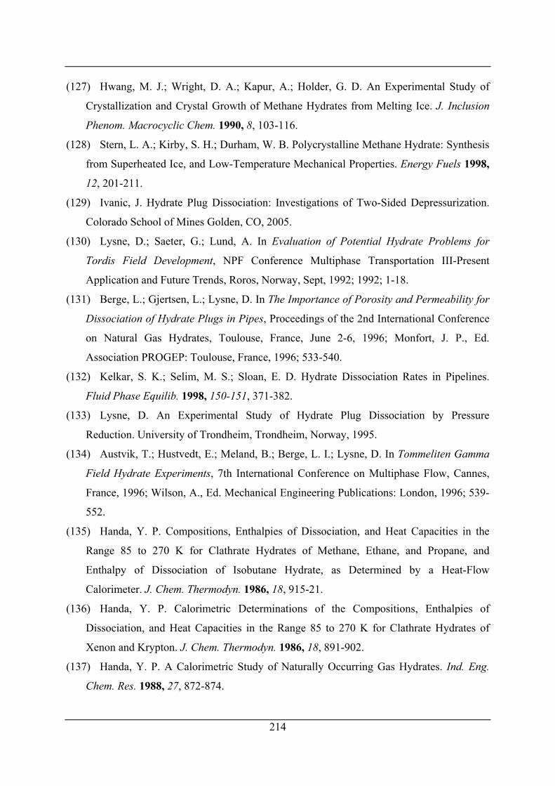
214
(127) Hwang, M. J.; Wright, D. A.; Kapur, A.; Holder, G. D. An Experimental Study of
Crystallization and Crystal Growth of Methane Hydrates from Melting Ice. J. Inclusion
Phenom. Macrocyclic Chem. 1990, 8, 103-116.
(128) Stern, L. A.; Kirby, S. H.; Durham, W. B. Polycrystalline Methane Hydrate: Synthesis
from Superheated Ice, and Low-Temperature Mechanical Properties. Energy Fuels 1998,
12, 201-211.
(129) Ivanic, J. Hydrate Plug Dissociation: Investigations of Two-Sided Depressurization.
Colorado School of Mines Golden, CO, 2005.
(130) Lysne, D.; Saeter, G.; Lund, A. In Evaluation of Potential Hydrate Problems for
Tordis Field Development, NPF Conference Multiphase Transportation III-Present
Application and Future Trends, Roros, Norway, Sept, 1992; 1992; 1-18.
(131) Berge, L.; Gjertsen, L.; Lysne, D. In The Importance of Porosity and Permeability for
Dissociation of Hydrate Plugs in Pipes, Proceedings of the 2nd International Conference
on Natural Gas Hydrates, Toulouse, France, June 2-6, 1996; Monfort, J. P., Ed.
Association PROGEP: Toulouse, France, 1996; 533-540.
(132) Kelkar, S. K.; Selim, M. S.; Sloan, E. D. Hydrate Dissociation Rates in Pipelines.
Fluid Phase Equilib. 1998, 150-151, 371-382.
(133) Lysne, D. An Experimental Study of Hydrate Plug Dissociation by Pressure
Reduction. University of Trondheim, Trondheim, Norway, 1995.
(134) Austvik, T.; Hustvedt, E.; Meland, B.; Berge, L. I.; Lysne, D. In Tommeliten Gamma
Field Hydrate Experiments, 7th International Conference on Multiphase Flow, Cannes,
France, 1996; Wilson, A., Ed. Mechanical Engineering Publications: London, 1996; 539-
552.
(135) Handa, Y. P. Compositions, Enthalpies of Dissociation, and Heat Capacities in the
Range 85 to 270 K for Clathrate Hydrates of Methane, Ethane, and Propane, and
Enthalpy of Dissociation of Isobutane Hydrate, as Determined by a Heat-Flow
Calorimeter. J. Chem. Thermodyn. 1986, 18, 915-21.
(136) Handa, Y. P. Calorimetric Determinations of the Compositions, Enthalpies of
Dissociation, and Heat Capacities in the Range 85 to 270 K for Clathrate Hydrates of
Xenon and Krypton. J. Chem. Thermodyn. 1986, 18, 891-902.
(137) Handa, Y. P. A Calorimetric Study of Naturally Occurring Gas Hydrates. Ind. Eng.
Chem. Res. 1988, 27, 872-874.
215
(138) Lievois, J. S.; Perkins, R.; Martin, R. J.; Kobayashi, R. Development of an Automated,
High Pressure Heat Flux Calorimeter and it Application to Measure the Heat of
Dissociation and Hydrate Numbers of Methane Hydrate. Fluid Phase Equilib. 1990, 59,
73-97.
(139) Rueff, R. M.; Sloan, E. D.; Yesavage, V. F. Heat Capacity and Heat of Dissociation of
Methane Hydrates. AIChE J. 1988, 34, 1468-76.
(140) Nagayev, V. B.; Gritsenko, A. I.; Murin, V. I. In Determination of Heat of CO2
Hydrate Formation, Transactions of the 8th All-Union Conference on Calorimetry and
Chemical Thermodynamics, Ivanovo, U.S.S.R, 1979; 1979; 58.
(141) Cherskii, N. V.; Groisman, A. G.; Nikitina, L. M.; Tsarev, V. P. Results of the First
Experimental Determination of Heats of Decomposition of Natural Gas Hydrates. Dokl.
Akad. Nauk SSSR 1982, 265, 185-9 [Geochem.].
(142) Kang, S. P.; Lee, H.; Ryu, B. J. Enthalpies of Dissociation of Clathrate Hydrates of
Carbon Dioxide, Nitrogen, (Carbon Dioxide + Nitrogen), and (Carbon Dioxide +
Nitrogen + Tetrahydrofuran). J. Chem. Thermodyn. 2001, 33, 513-521.
(143) Marsh, K. N.; Gao, J. Enthalpies of Formation of Gas Hydrates. Annual Convention
Proceedings - Gas Processors Association 2004, 83, 1-10.
(144) Handa, Y. P.; Hawkins, R. E.; Murray, J. J. Calibration and Testing of a Tian-Calvet
Heat-Flow Calorimeter. Enthalpies of Fusion and Heat Capacities for Ice and
Tetrahydrofuran Hydrate in the Range 85 to 270 K. J. Chem. Thermodyn. 1984, 16, 623-
32.
(145) Levik, O. I. Thermophysical and Composition Properties of Natural Gas Hydrates.
Norwegian University of Science and Technology, Trondheim, Norway, 2000.
(146) Rydzy, M. B.; Schicks, J. M.; Naumann, R.; Erzinger, J. Dissociation Enthalpies of
Synthesized Multicomponent Gas Hydrates with Respect to the Guest Composition and
Cage Occupancy. J. Phys. Chem. B 2007, 111, 9539-9545.
(147) Anderson, G. K. Enthalpy of Dissociation and Hydration Number of Carbon Dioxide
Hydrate from the Clapeyron Equation. J. Chem. Thermodyn. 2003, 35, 1171-1183.
(148) van der Waals, J. H.; Platteeuw, J. C. Validity of Clapeyrons Equation for Phase
Equilibria Involving Clathrates. Nature 1959, 183, 462-462.
(149) Barrer, R. M.; Stuart, W. I. Non-Stoicheiometric Clathrate Compounds of Water.
Proc. R. Soc. London, A 1957, 243, 172-189.
216
(150) Glew, D. N. Some Stocheiometric Gas Hydrates. Nature 1959, 184, 545-546.
(151) Roberts, O. L.; Brownscombe, E. R.; Howe, L. S. Methane and Ethane Hydrates. Oil
Gas J. 1940, 39, 37-42.
(152) Barrer, R. M.; Edge, A. V. J. Gas Hydrates Containing Argon, Krypton and Xenon:
Kinetics and Energetics of Formation and Equilibria. Proc. R. Soc. London, A 1967, 300,
1-24.
(153) Skovborg, P.; Rasmussen, P. Comments on: Hydrate dissociation enthalpy and guest
size. Fluid Phase Equilib. 1994, 96, 223-231.
(154) Sloan, E. D.; Fleyfel, F. Hydrate Dissociation Enthalpy and Guest Size. Fluid Phase
Equilib. 1992, 76, 123-40.
(155) Sloan, E. D.; Fleyfel, F. Reply to "Comments on: Hydrate Dissociation Enthalpy and
Guest Size". Fluid Phase Equilib. 1994, 96, 233-5.
(156) Anderson, G. K. Enthalpy of Dissociation and Hydration Number of Methane Hydrate
from the Clapeyron Equation. J. Chem. Thermodyn. 2004, 36, 1119-1127.
(157) Glew, D. N. Aqueous Nonelectrolyte Solutions. Part XVIII. Equilibrium Pressures of
Two Methane Hydrates With Water. Formulae and Dissociation Thermodynamic
Functions for the Structures I and II Methane Hydrates. Can. J. Chem. 2002, 80, 418-439.
(158) Yoon, J.-H.; Yamamoto, Y.; Komai, T.; Haneda, H.; Kawamura, T. Rigorous
Approach to the Prediction of the Heat of Dissociation of Gas Hydrates. Ind. Eng. Chem.
Res. 2003, 42, 1111-1114.
(159) Bollavaram, P.; Sloan, E. D. In Pipeline Hydrate Dissociation: Effects of Crystal
Structure, Proc. 4th International Conference on Gas Hydrates, Yokohama, Japan, May
19-23, 2002; Mori, Y. H., Ed. 2002; 947-951.
(160) Wilcox, W. I.; Carson, D. B.; Katz, D. L. Natural Gas Hydrates. Ind. Eng. Chem.
1941, 33, 662-665.
(161) Carson, D. B.; Katz, D. L. Natural Gas Hydrates. Trans. AIME 1942, 146, 150-158.
(162) Happel, J.; Hnatow, M. A.; Meyer, H. The Study of Separation of Nitrogen from
Methane by Hydrate Formation Using a Novel Apparatus. Ann. N. Y. Acad. Sci. 1994,
715, 412-424.
(163) Kini, R. A. NMR Studies of CH4, C2H6, and C3H8 Hydrates: Structure, Kinetics, and
Thermodynamics. Colorado School of Mines, Golden, Co, 2002.
217
(164) Fleyfel, F.; Devlin, J. P. Carbon Dioxide Clathrate Hydrate Epitaxial Growth:
Spectroscopic Evidence for Formation of the Simple Type-II Carbon Dioxide Hydrate. J.
Phys. Chem. 1991, 95, 3811-3815.
(165) Staykova, D. K.; Kuhs, W. F.; Salamatin, A. N.; Hansen, T. Formation of Porous Gas
Hydrates from Ice Powders: Diffraction Experiments and Multistage Model J. Phys.
Chem. B 2003, 107, 10299-10311.
(166) Schicks, J. M.; Ripmeester John, A. The Coexistence of Two Different Methane
Hydrate Phases under Moderate Pressure and Temperature Conditions: Kinetic versus
Thermodynamic Products. Angew. Chem., Int. Ed. 2004, 43, 3310-3313.
(167) Schicks, J. M.; Naumann, R.; Erzinger, J.; Hester, K. C.; Koh, C. A.; Sloan, E. D.
Phase Transitions in Mixed Gas Hydrates: Experimental Observations versus Calculated
Data J. Phys. Chem. B 2006, 110, 11468-11474.
(168) Lemmon, E. W.; Huber, M. L.; McLinden, M. O. NIST Standard Reference Database
23: Reference Fluid Thermodynamic and Transport Properties-REFPROP, 7.1; National
Institute of Standards and Technology: Gaithersburg, MD, 2003.
(169) Kamata, Y.; Yamakoshi, Y.; Ebinuma, T.; Oyama, H.; Shimada, W.; Narita, H.
Hydrogen Sulfide Separation Using Tetra-n-butyl Ammonium Bromide Semi-clathrate
(TBAB) Hydrate. Energy Fuels 2008, 19, 1717-1722.
(170) Tohidi, B.; Burgass, R. W.; Danesh, A.; Østergaard, K. K.; Todd, A. C. Improving the
Accuracy of Gas Hydrate Dissociation Point Measurements. Ann. N. Y. Acad. Sci. 2000,
912, 924-931.
(171) Mao, W. L.; Mao, H.-K.; Goncharov, A. F.; Struzhkin, V. V.; Guo, Q.; Hu, J.; Shu, J.;
Hemley, R. J.; Somayazulu, M.; Zhao, Y. Hydrogen Clusters in Clathrate Hydrate.
Science 2002, 297, 2247-9.
(172) Lipkowski, J.; Komarov, V. Y.; Rodionova, T. V.; Dyadin, Y. A.; Aladko, L. S. The
Structure of Tetra-Butyl-Ammonium Bromide Hydrate (C4H9)4NBr·21/3H2O. J.
Supramol. Chem. 2002, 2, 435-439.
(173) Darbouret, M.; Cournil, M.; Herri, J. M. In Rheological Study of a Hydrate Slurry for
Air Condtioning Applications, Proceedings of the Fifth International Conference on Gas
Hydrates, Trondheim, Norway, Jun 12-16, 2005; 2005.
218
(174) Tohidi, B.; Danesh, A.; Todd, A. C. Modelling Single and Mixed Electrolyte
Solutions and its Applications to Gas Hydrates. Chem. Eng. Res. Des. 1995, 73A, 464-
472.
(175) Tohidi-Kalorazi, B. Gas Hydrate Equilibria in the Presence of Electrolyte Solutions.
Herriot-Watt University, Edinburgh, U.K, 1995.
(176) Strobel, T. A.; Koh, C. A.; Sloan, E. D. Hydrogen Storage Properties of Clathrate
Hydrate Materials. Fluid Phase Equilib. 2007, 261, 382-389.
(177) Ahmadloo, F.; Mali, G.; Chapoy, A.; Tohidi, B. In Gas Separation and Storage Using
Semi-Clathrate Hydrates, Proceedings of the 6th International Conference on Gas
Hydrates, Vancouver, Canada, July 6-10, 2008; University of British Columbia
Information Repository (circle.ubc.ca), 2008.
(178) Gudmundsson, J. S.; Andersson, V.; Dugut, I.; Levik, O. I.; Mork, M. In NGH on
FPSO - Slurry Process and Cost Estimate, Proceedings of the SPE Annual Technical
Conference, Houston, Tx, October 3-6, 1999; 1999.
(179) Gudmundsson, J. S.; Andersson, V.; Levik, O. I. In Gas Storage and Transport Using
Hydrates, Proceedings of the Offshore Mediterranean Conference, Ravenna, Italy, Mar
19-21, 1997; 1997.
(180) Gudmundsson, J. S.; Børrehaug, A. Natural Gas Hydrate - An Alternative to Liquefied
Natural gas. Petrol. Rev. 1996, 50, 232-235.
(181) Gudmundsson, J. S.; Graff, O. F. In Hydrate Non-Pipeline Technology for Transport
of Natural Gas, Proceedings of the 22nd World Gas Conference, Tokyo, Japan, June 1-5,
2003; 2003.
(182) Gudmundsson, J. S.; Mork, M. In Stranded Gas to Hydrate for Storage and Transport,
2001 International Gas Research Conference, Amsterdam, Netherlands, November 5-8,
2001; 2001.
(183) Gudmundsson, J. S.; Mork, M.; Graff, O. F. In Hydrate Non-Pipeline Technology,
Proceedings of the 4th International Conference on Gas Hydrates, Yokohama, Japan,
May 19-23, 2002; 2002.
(184) Yakushev, V. S.; Istomin, V. A. Gas-Hydrates Self-Preservation Effect. In Physics
and Chemistry of Ice, Maeno, N.; Hondoh, T., Eds.; Hokkaido Univ. Press: Sapporo,
Japan, 1992; pp 136-139.
219
(185) Gudmundsson, J. S.; Parlaktuna, M.; Khokar, A. A. Storing Natural Gas as Frozen
Hydrate. SPE Prod. Facil. 1994, 9, 69-73.
(186) Børrehaug, A.; Gudmundsson, J. S. In Gas Transportation in Hydrate Form,
EUROGAS 96, Trondheim, Norway, 3-5 Jun, 1996; 1996; 35-41.
(187) Gudmundsson, J. S.; Andersson, V.; Levik, O. I.; Mork, M. Hydrate Technology for
Capturing Stranded Gas. Ann. N. Y. Acad. Sci. 1999, 912, 403-410.
(188) Hove, A. M.; G, L.; Gudmundsson, J. S. In NGT Technology - A Promising Concept
for Gas Storage and Transport, Proceedings of Gas to Liquids II, London, UK, Sep 22-
23, 1999; 1999.
(189) Tse, J. S. Thermal Expansion of the Clathrate Hydrates of Ethylene Oxide and
Tetrahydrofuran. J. Phys. Colloques 1987, 48, C1-543-C1-549.
(190) Stern, L. A.; Circone, S.; Kirby, K. B.; Durham, W. B. Temperature, Pressure, and
Compositional Effects on Anomalous or "Self" Preservation of Gas Hydrates. Can. J.
Phys. 2003, 81, 271-283.
(191) Ohtani, N.; Yamashita, T.; Hosoda, Y. Phase Behavior of Tetrabutylammonium
Salt/Oil/Water/Inorganic Salt Four-Component Systems. Bull. Chem. Soc. Jpn. 2000, 73,
2269-2277.
(192) Aladko, L. S.; Dyadin, Y. A.; Mikina, T. V. Diisoamyldibutylammonium Bromide
Clathrate Hydrates. Russ. J. Gen. Chem. 2002, 72, 364-367.
(193) Owe Berg, T. G. Liquid Structure and Solubility of Sparingly Soluble Salts in Water.
Acta Chem. Scand. 1953, 7, 1313-1322.
(194) Sharma, R. K.; Fry, J. L. Instability of Anhydrous Tetra-n-alkylammonium Fluorides.
J. Org. Chem. 1983, 48, 2112-2114.
(195) Kamata, Y.; Yamakoshi, Y.; Ebinuma, T.; Oyama, H.; Shimada, W.; Narita, H.
Hydrogen Sulfide Separation Using Tetra-n-butyl Ammonium Bromide Semi-clathrate
(TBAB) Hydrate. Energy Fuels 2005, 19, 1717-1722.
(196) Huheey, J.; Keiter, E. A.; Keiter, R. L. Inorganic Chemistry, Principles of Structure
and Reactivity. 4th ed.; Harper Collins: New York, 1993.
(197) Wells, A. F. Structural Inorganic Chemistry. 5th ed.; Oxford University Press:
Oxford, U.K., 1984.
(198) Ferraro, J. R.; Nakamoto, K.; Brown, C. W. Introductory Raman Spectroscopy. 2nd
ed.; Academic Press: Amsterdam, 2003.
220
(199) Laugier, J.; Bochu, B. GRETEP v2: Grenoble Thermal Ellipsoids Plot Program
(Downloadable from http://www.ccp14.ac.uk/ccp/web-mirrors/lmgp-laugier-
bochu/gretep.zip), Laboratoire des Matériaux et du Génie Physique, Ecole Nationale
Supérieure de Physique de Grenoble (INPG): 2003.
(200) Macrae, C. F.; Edgington, P. R.; McCabe, P.; Pidcock, E.; Shields, G. P.; Taylor, R.;
Towler, M.; van de Streek, J. Mercury 1.4.2 (build 2) (Downloadable from
http://www.ccdc.cam.ac.uk/free_services/mercury/downloads/Mercury_1.4.2/mercury_1_
4_2.exe), The Cambridge Crystallographic Data Centre: 2007.
(201) Schuster, C. E. ExxonMobil High-Pressure Process Technology for LDPE. In
Handbook of Petrochemicals Production Processes, 1st ed.; Meyers, R. A., Ed. McGraw
Hill: New York, 2005; pp 14.45-14.58.
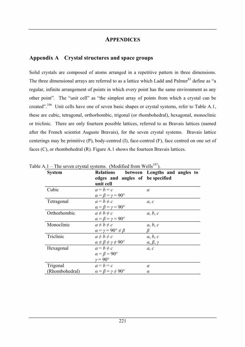
221
APPENDICES Appendix A Crystal structures and space groups
Solid crystals are composed of atoms arranged in a repetitive pattern in three dimensions.
The three dimensional arrays are referred to as a lattice which Ladd and Palmer83 define as “a
regular, infinite arrangement of points in which every point has the same environment as any
other point”. The “unit cell” as “the simplest array of points from which a crystal can be
created”.196 Unit cells have one of seven basic shapes or crystal systems, refer to Table A.1,
these are cubic, tetragonal, orthorhombic, trigonal (or rhombohedral), hexagonal, monoclinic
or triclinic. There are only fourteen possible lattices, referred to as Bravais lattices (named
after the French scientist Auguste Bravais), for the seven crystal systems. Bravais lattice
centerings may be primitive (P), body-centred (I), face-centred (F), face centred on one set of
faces (C), or rhombohedral (R). Figure A.1 shows the fourteen Bravais lattices.
Table A.1 – The seven crystal systems. (Modified from Wells197). System Relations between
edges and angles of unit cell
Lengths and angles to be specified
Cubic a = b = c α = β = γ = 90°
a
Tetragonal a = b ≠ c α = β = γ = 90°
a, c
Orthorhombic a ≠ b ≠ c α = β = γ = 90°
a, b, c
Monoclinic a ≠ b ≠ c α = γ = 90° ≠ β
a, b, c β
Triclinic a ≠ b ≠ c α ≠ β ≠ γ ≠ 90°
a, b, c α, β, γ
Hexagonal a = b ≠ c α = β = 90° γ = 90°
a, c
Trigonal (Rhombohedral)
a = b = c α = β = γ ≠ 90°
a α
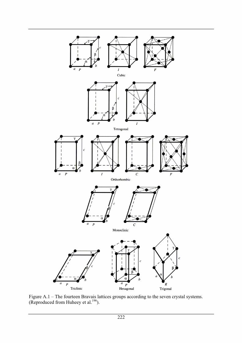
Figure A.1 – The fourteen Bravais lattices groups according to the seven crystal systems. (Reproduced from Huheey et al.196).
222
223
The unit cell can be defined as the smallest unit that can generate the crystal structure with
only translation operations. The asymmetric unit on the other hand is the smallest unit upon
which symmetry operations will allow the unit cell to be generated. Space groups in the
commonly used Hermann-Mauguin notation describe both the centrings of the lattice in terms
of P, I, F, C or R as well as the symmetry operations that are required to generate the unit cell
from the asymmetric unit. The space group symbolism is described in Table A.2 the first
symbol is the lattice centring, the second the principal axis, further symbols may describe
axes of rotation, screw axes, mirror planes or glide planes. A detailed description of these
symmetry operations may be found in Ladd and Palmer,83 Huheey et al.196 or Ferraro et al.198
Table A.2 – Hermann-Manguin space group symbolism. (Modified from Ferraro et al.198). First symbol refers to the Bravais lattice P = primitive C = centred lattice F = face centred I = body centred R = rhombohedral Principal axis of ration given number n = order e.g., 2 = twofold axis of rotation For screw axis, np: n = order of axis, p/n = fraction of primitive lattice over which translation parallel to screw axis occurs e.g., P21 = primitive lattice with a twofold axis of rotation, translation, one-half unit cell Mirror plane = m Glide planes = symbols a, b, c along (a), (b), (c) axes symbol n = (b + c)/2 or (a + b)/2 symbol d = (a + b)/4 or (b + c)/4 or (a + c)/4 e.g. P21/m; = mirror plane perpendicular to the principal axis* C2/c; = glide plane axis perpendicular to principal axis* * The slash indicates the glide plane is perpendicular to the principal axis (if a slash is not present the glide plane is parallel to the principal axis)
The specification of the coordinates of atoms of the asymmetric unit, the space group and the
unit cell parameters (a, b and c) fully define the crystal structure. If the asymmetric unit
coordinates are expressed in fractions of the unit cell parameters, x, y and z, then space groups
allow the generation of a set of positions based on the asymmetric unit coordinates generally
described by (±x ± fx, ±y ± fy, ±z ± fz), where fx, fy, fz are a fraction of the unit cell parameter in
the parameters and may differ for each generated set of position (and may be equal to zero).
Some example of these can be seen in the sixth column of Table B.1.
Appendix B Size calculation of 4454 cage of tetraisopentylammonium fluoride, TIPAF·27H2O The size of a 4454 cage was calculated from Lipkowski et al.’s67 crystallographic data for
tetraisopentylammonium fluoride with 27 waters of hydration (TIPAF·27H2O). The data was
initially entered into the computer program GRETEP v2 199 and was then exported via a CIF
(crystallographic information file) to Mercury 1.4.2 200 for visualisation, a partially visible
5444 cage was expanded and its twelve vertices (oxygen atoms) were selected. A centroid was
produced at the centre of the twelve oxygen atoms (at fractional coordinates xfr = 0.5, yfr =
0.25, zfr = 0.875). The generated atoms were then exported to Microsoft Excel where the
distance between each atom and the centroid was calculated. The distance of each oxygen
atom from the centroid was calculated using the formula ( ) ( ) ( )2 2fr fr frd a x b y c z= Δ + Δ + Δ 2 ,
where d is the distance, a, b and c are the lattice parameters, and Δxfr, Δyfr, and Δzfr are the
deviations of the fractional coordinates of each oxygen atom from the centroid. The distances
to the centre of the cage (or centroid) are listed in Table B.1, giving a mean value of 3.331 Å.
Using the van der Waals radius of oxygen of 1.4 Å that Davidson11 used to calculate the mean
“free diameters” of the 512, 51262 and 51264 cages of sI and sII hydrate the mean “free
diameter” of the 5444 cage is 3.9 Å (2×3.331 - 2×1.4). This indicates that molecules the size
of Argon (largest van der Waals diameter = 3.8 Å)11 and smaller molecules such as hydrogen,
helium and neon could fit inside the cage. Slightly larger molecules on the other hand such as
krypton and oxygen both with a largest van der Waals diameter of 4.0 Å 11 as well as
methane, nitrogen, hydrogen sulfide, each with a largest van der Waals diameter of 4.1 Å 11
could probably not fit unless the cage was able to expand slightly to accommodate these
larger molecules. The non-spherical nature of the cage may also mean that only appropriately
shaped molecules may fit, however this is probably only important when the molecule’s
largest van der Waals diameter approaches 3.9 Å. One way to quantify the non-sphericity of
a cage is to compare the maximum and minimum distances of atoms that make up the vertices
of a cage to the mean value for all the atoms. Deviations of the maximum and minimum
distances from the cage centre to the cage atoms relative to the mean distance from the cage
centre to cage atoms are presented in Table B.2. Data for sI 512, sII 512, sI 51262 and sII 51264
are compared to that for the 4454 cage. It is clear that the 4454 is the most non-spherical cage
by a large margin, with distance to the centre of the cage deviating from the mean value by
224
approximately ± 15 %, compared to the next value of greatest magnitude of 7.3 % for the sII
51262 cage.
Table B.1 – Generated atoms making up a 5444 cage.a Labelb xfr yfr zfr d/Å Symm. op.b
O1 0.3672 0.1741 0.8075 2.830 1.25-y,-1/4+x,3/4+z O1 0.4241 0.3828 0.9425 2.830 x,-1/2+y,1-z O1 0.5759 0.1172 0.9425 2.830 1-x,1-y,1-z O1 0.6328 0.3259 0.8075 2.830 -1/4+y,3/4-x,3/4+z O2 0.4171 0.2628 1.0513 3.333 1-x,1/2-y,1+z O2 0.4872 0.1671 0.6987 3.333 1/4+y,3/4-x,3/4-z O2 0.5128 0.3329 0.6987 3.333 3/4-y,-1/4+x,3/4-z O2 0.5829 0.2372 1.0513 3.333 x,y,1+z O4 0.378 0.3398 0.7086 3.828 1/4+y,3/4-x,3/4-z O4 0.4102 0.128 1.0414 3.828 x,y,1+z O4 0.5898 0.372 1.0414 3.828 1-x,1/2-y,1+z O4 0.622 0.1602 0.7086 3.828 3/4-y,-1/4+x,3/4-z
a Atoms generated from data of Lipkowski et al.67 for TIPAF·27H2O, all values/entries except
distances, d, are from Mercury 1.4.2.200 Fractional coordinates of the atoms in the unit cell,
xfr, yfr and zfr ( fr fr fr/ , / , /x x a y y b z z c= = = , where a, b and c are the lattice parameters) are
listed for the atoms generated from the labelled oxygen atom in the first column generated
using the symmetry operation in the “Symm. Op.” column. For Lipkowski et al.’s67
TIPAF·27H2O structure the lattice parameters at -50 °C where used: a = b = 16.894 Å, c =
17.111 Å. (tetragonal), using the parameters at 0 °C generated d values of 2.838 Å, 3.342 Å
and 3.839 Å and a mean free cage diameter that was 0.02 Å larger (3.88 Å versus 3.86 Å) b Labelled oxygen atoms using the numbering of Lipkowski et al.67, the symmetry operations
to generate the positions listed are in the sixth column of the table labelled “Symm. Op.”.
Table B.2 – Comparison of sphericity of cages.a Distances from cage centre /Å sI 512 sII 512 sI 51262 sII 51264 4454
max. 3.96 3.748 4.645 4.729 3.828 min. 3.83 3.956 4.06 4.635 2.830 mean 3.91 3.902 4.33 4.683 3.331
Percentage deviations from mean value sI 512 sII 512 sI 51262 sII 51264 4454
max dev. 1.3% -3.9% 7.3% 1.0% 14.9% min dev. -2.0% 1.4% -6.2% -1.0% -15.0%
a Data for cages other than 4454 from table II of Davidson.11
225
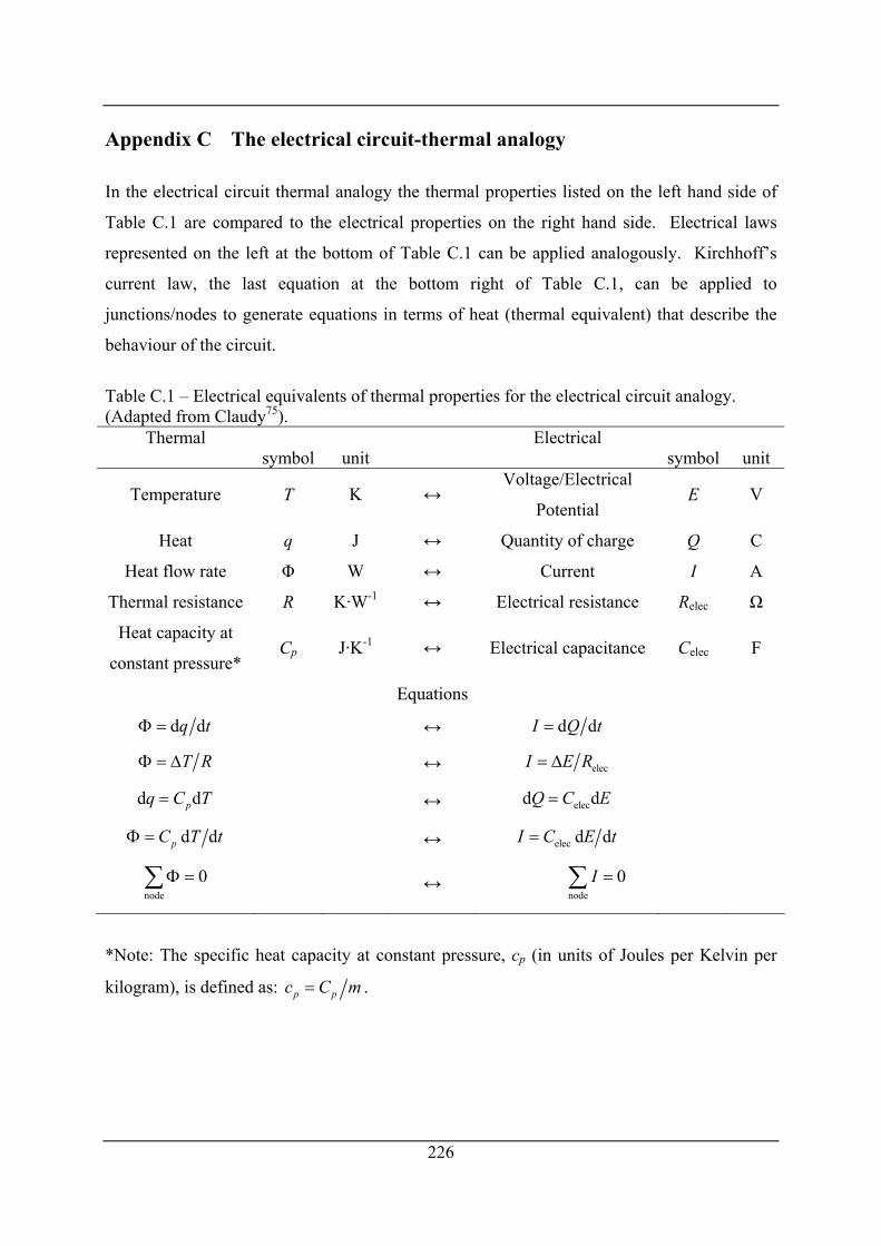
Appendix C The electrical circuit-thermal analogy
In the electrical circuit thermal analogy the thermal properties listed on the left hand side of
Table C.1 are compared to the electrical properties on the right hand side. Electrical laws
represented on the left at the bottom of Table C.1 can be applied analogously. Kirchhoff’s
current law, the last equation at the bottom right of Table C.1, can be applied to
junctions/nodes to generate equations in terms of heat (thermal equivalent) that describe the
behaviour of the circuit.
Table C.1 – Electrical equivalents of thermal properties for the electrical circuit analogy. (Adapted from Claudy75).
Thermal Electrical symbol unit symbol unit
Temperature T K ↔ Voltage/Electrical
Potential E V
Heat q J ↔ Quantity of charge Q C
Heat flow rate Φ W ↔ Current I A
Thermal resistance R K·W-1 ↔ Electrical resistance Relec Ω
Heat capacity at
constant pressure* Cp J·K-1 ↔ Electrical capacitance Celec F
Equations
d dq tΦ = ↔ d dI Q t=
T RΦ = Δ ↔ elecI E R= Δ
d dpq C T= ↔ elecd dQ C E=
d dpC T tΦ = ↔ elec d dI C E t=
node0Φ =∑ ↔
node0I =∑
*Note: The specific heat capacity at constant pressure, cp (in units of Joules per Kelvin per
kilogram), is defined as: p pc C m= .
226
Appendix D Mole balance on hydrate dissociation
Hydrate dissociation can be represented by the equation:
, (A.1) 2 V AqG· H O V Aqn N N→ +
where G represents the hydrate guest, n the hydrate number (moles of water per mole of
guest), V represents the vapour phase, NV represents the moles of vapour phase (subscript V =
vapour phase), Aq represents the aqueous phase and NAq represents the moles of aqueous
phase (subscript Aq = aqueous phase).
If a mole balance is performed based on eq (A.1) then for the guest:
G GV V Aq Aq1 x N x N= + , (A.2)
where GVx is the mole fraction of the guest in the vapour phase and G
Aqx is the mole fraction of
the guest in the aqueous phase. A similar mole balance may be performed on the water:
, (A.3) 2 2H O H OV V Aq Aqn x N x N= +
where 2H OVx is the mole fraction of water in the vapour phase and 2H O
Aqx is the mole fraction of
water in the aqueous phase.
Solving eqs (A.2) and (A.3) simultaneously leads to:
( ) 2
2
H OV
Aq H O GV Aq
11n n x
Nx x
− +=
− −, (A.4)
and
227
( )
2
GAq
V H O GV A
1 11
n xN
qx x− +
=− −
. (A.5)
These equations have been defined in terms of the mole fractions that tend towards zero under
the “idealised conditions” of no solubility of the guest in water and no vaporisation of the
water in to the vapour phase. So by setting 2H OV 0x = and G
Aq 0x = the result is:
AqN n= , (A.6)
and
V 1N = . (A.7)
Using eqs (A.6) and (A.7) in eq (A.1) the following is obtained:
, (A.8) 2G· H O G H On n→ + 2
otherwise for non-idealised conditions:
( ) ( ) 2
2 2
G H OAq V
2 H OH O G GV Aq V Aq
1 1 1M· H O V Aq
1 1n x n n x
nx x x x
⎡ ⎤ ⎡− + − +→ +⎢ ⎥ ⎢
− − − −⎢ ⎥ ⎢⎣ ⎦ ⎣
⎤⎥⎥⎦
. (A.9)
Anderson (eq 6, p1175),147 uses the following equation for the volume difference:
GAq
Aq HGAq
11 V
nxV V nV
x⎡ ⎤
Δ = − + −⎢ ⎥−⎢ ⎥⎣ ⎦
V . (A.10)
From eq (A.5) for the moles of vapour if it is assumed that 2H OV 0x = (no vaporisation of
water) then:
228
( ) ( )
2
G G M GAq Aq Aq Aq Aq
V H O G G G GV Aq Aq Aq A
1 1 1 1 11
1 1 1n x n x x nx nx
NG
q1x x x x− + − + − −
= = = = −− − − − − x
, (A.11)
which is the same as what Anderson has used in eq (A.10).
From eq (A.4) for the mole of aqueous solution if it is assumed that then: 2H OV 0x =
( ) 2
2
H OV
Aq H O GV Aq A
11 1n n x nN G
qx x x− +
= =− − −
, (A.12)
Anderson neglects the G
Aqx in the denominator for the aqueous volume and gives eq (A.6).
229
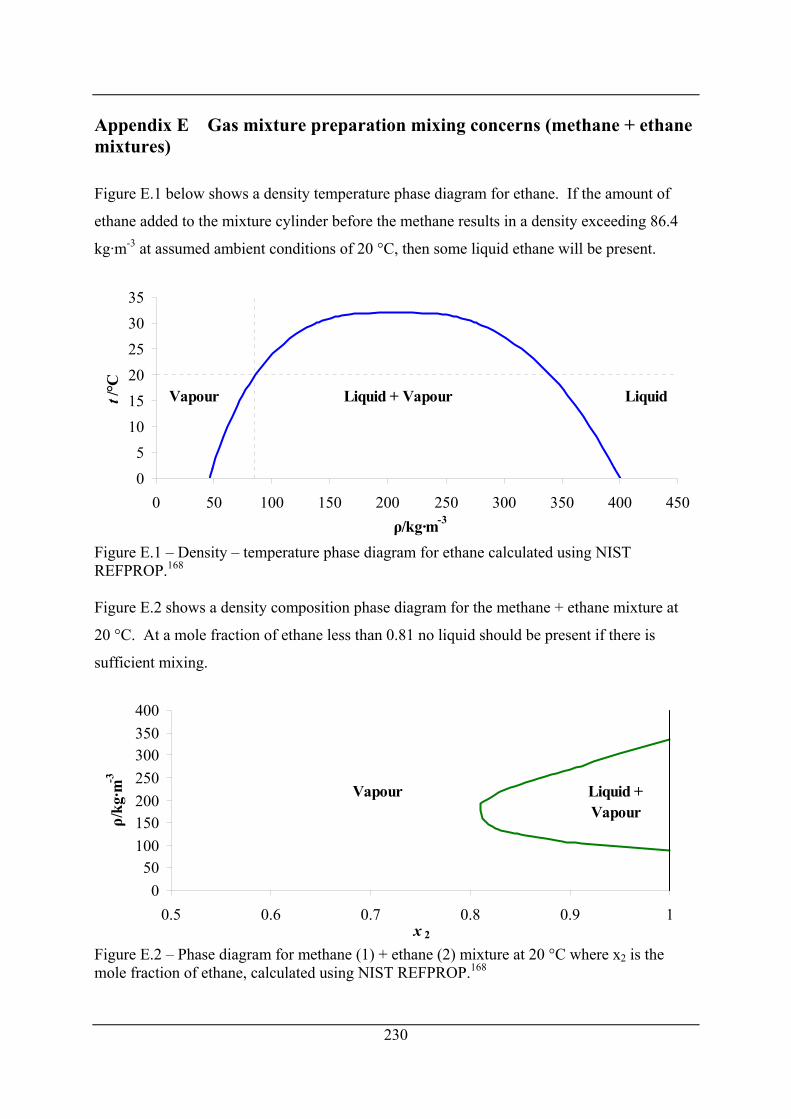
Appendix E Gas mixture preparation mixing concerns (methane + ethane mixtures)
Figure E.1 below shows a density temperature phase diagram for ethane. If the amount of
ethane added to the mixture cylinder before the methane results in a density exceeding 86.4
kg·m-3 at assumed ambient conditions of 20 °C, then some liquid ethane will be present.
05
101520253035
0 50 100 150 200 250 300 350 400 450ρ/kg·m-3
t/°C LiquidLiquid + VapourVapour
Figure E.1 – Density – temperature phase diagram for ethane calculated using NIST REFPROP.168
Figure E.2 shows a density composition phase diagram for the methane + ethane mixture at
20 °C. At a mole fraction of ethane less than 0.81 no liquid should be present if there is
sufficient mixing.
050
100150200250300350400
0.5 0.6 0.7 0.8 0.9 1x 2
ρ/kg
·m-3
Liquid +Vapour
Vapour
Figure E.2 – Phase diagram for methane (1) + ethane (2) mixture at 20 °C where x2 is the mole fraction of ethane, calculated using NIST REFPROP.168
230
Appendix F ISCO pump gas mixture calculations
The initial molar density, ρmix,i, of the mixture of methane (1) + ethane (2) was calculated in
NIST Refprop168 from the known initial mole fractions of each component of the gas (x1,i,
x2,i), P and T, the moles of methane and ethane were then individually calculated using eq
(A.13), where j represents the component number, by guessing an initial volume of gas to
charge the ISCO pump with, Vi:
j,i j,i mix,i in x Vρ= . (A.13)
Then using the final desired gas composition (x1,f, x2,f), P and T, it was possibly to work out
the final molar density of the mixture, ρmix,f, in NIST Refprop. Using this molar density and
the ISCO pump maximum volume of 266 ml as the final mixture volume, Vf, it was possible
to calculate the final moles of methane, n1,f using eq (A.14). The initial volume, Vi, was then
iterated until the final calculated composition of methane in the gas, x1,f, from eq (A.15)
matched the final desired composition.
1,f 1,f mix,f fn x Vρ= . (A.14)
1,f1,f
1,f 2,i
nx
n n=
+. (A.15)
231
232
Appendix G Hydraulic pressure testing of constructed cells
Hydraulic pressure testing was carried out on the long cell and short cell that were constructed
for plug dissociation measurements at the University of Canterbury. Water was used as the
test fluid and a screw piston pump type pressure generator with a maximum operating
pressure of 103.4 MPa (15000 psi) obtained from HiP (High Pressure Equipment Company
model number 50-6-15) was used to pressurise the cells. The system is shown in Figure G.1.
The system was initially started with both valves 1 and 2 closed. The cell was attached to the
system then held in an upright position by clamping it to a retort stand. A plug fitting at the
top of the cell was removed and the cell was filled completely with water. The system was
gently rocked and allowed to stand for half an hour so that any air bubbles would rise to the
top. The system was then topped up with water again and the plug fitting was replaced and
tightened. Water was then drawn in to the screw piston pump by opening valve 1 and rotating
the handle counter clockwise until fully extended. Valve 1 was then closed and valve 2
opened. The pumps handle was then rotated in a clockwise direction and the rising pressure
was monitored on the pressure gauge (Heise CM-18357). When the handle reached zero
extension the system pressure was noted, valve 2 was closed, and valve 1 opened. The pump
was refilled with water by rotating the handle counter clockwise to maximum extension.
Valve 1 was then closed. The pump handle was then rotated clockwise until the pressure
reached approximately the same pressure as before the pump was refilled, then valve 2 was
opened. This was done to minimize the pressure shock on the cell. When the pressure
reached 70 MPa (10150 psi) pumping was stopped and the system was allowed to rest for 1
hour. To depressurize the system the handle was wound back. When the handle reached full
extension the pressure in the system was noted valve 2 was shut and valve 1 opened. The
pump handle was then rotated clockwise to about half extension then valve 1 was shut. The
system up to valve 2 was then repressurized to the approximate pressure in the cell and valve
2 was opened. Depressurization then continued by rotating the handle counter clockwise until
the pressure in the cell dropped to atmospheric.
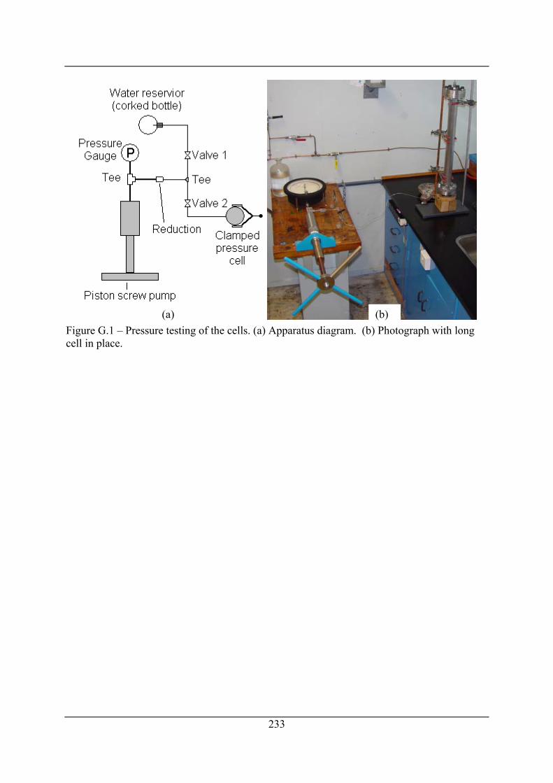
233
Figure G.1 – Pressure testing of the cells. (a) Apparatus diagram. (b) Photograph with long cell in place.
(a) (b)
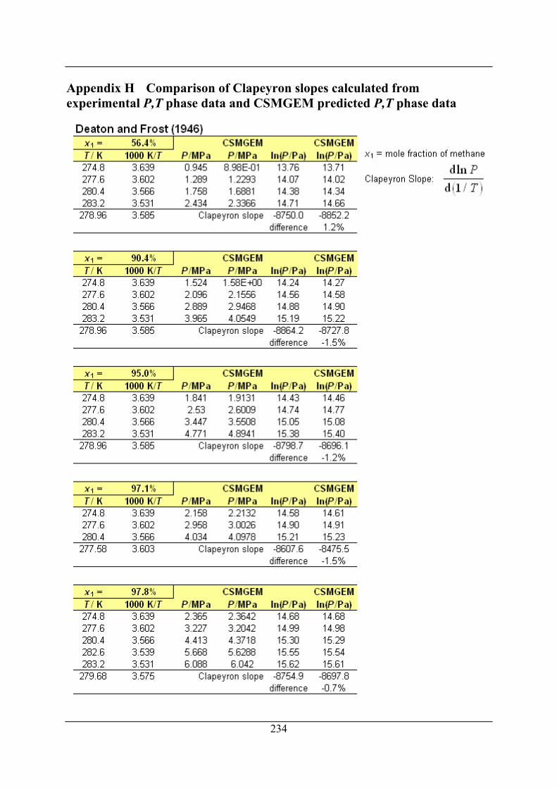
Appendix H Comparison of Clapeyron slopes calculated from experimental P,T phase data and CSMGEM predicted P,T phase data
234
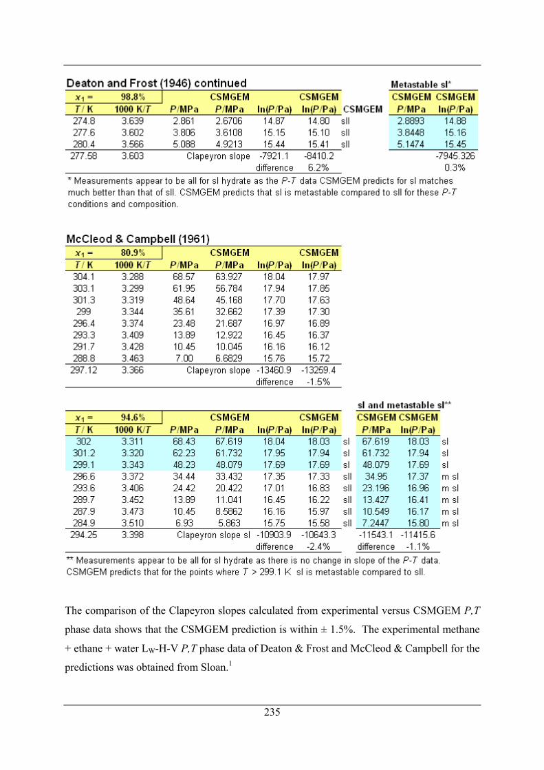
The comparison of the Clapeyron slopes calculated from experimental versus CSMGEM P,T
phase data shows that the CSMGEM prediction is within ± 1.5%. The experimental methane
+ ethane + water LW-H-V P,T phase data of Deaton & Frost and McCleod & Campbell for the
predictions was obtained from Sloan.1
235
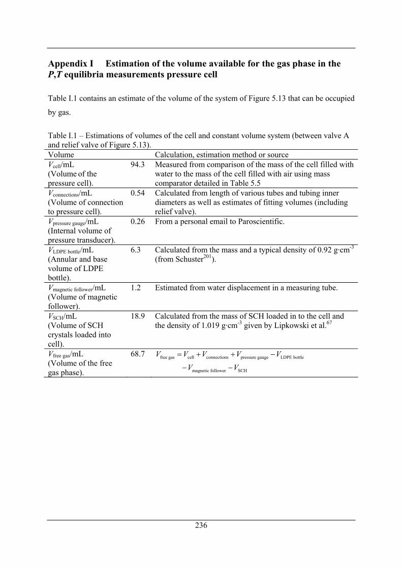
Appendix I Estimation of the volume available for the gas phase in the P,T equilibria measurements pressure cell
Table I.1 contains an estimate of the volume of the system of Figure 5.13 that can be occupied
by gas.
Table I.1 – Estimations of volumes of the cell and constant volume system (between valve A and relief valve of Figure 5.13). Volume Calculation, estimation method or source Vcell/mL (Volume of the pressure cell).
94.3 Measured from comparison of the mass of the cell filled with water to the mass of the cell filled with air using mass comparator detailed in Table 5.5
Vconnections/mL (Volume of connection to pressure cell).
0.54 Calculated from length of various tubes and tubing inner diameters as well as estimates of fitting volumes (including relief valve).
Vpressure gauge/mL (Internal volume of pressure transducer).
0.26 From a personal email to Paroscientific.
VLDPE bottle/mL (Annular and base volume of LDPE bottle).
6.3 Calculated from the mass and a typical density of 0.92 g·cm-3 (from Schuster201).
Vmagnetic follower/mL (Volume of magnetic follower).
1.2 Estimated from water displacement in a measuring tube.
VSCH/mL (Volume of SCH crystals loaded into cell).
18.9 Calculated from the mass of SCH loaded in to the cell and the density of 1.019 g·cm-3 given by Lipkowski et al.67
Vfree gas/mL (Volume of the free gas phase).
68.7 free gas cell connections pressure gauge LDPE bottle
magnetic follower SCH
V V V V V
V V
= + + −
− −
236

![New Techniques in Corolling Gas Hydrates [Recovered] Techniques in Corolling Gas Hydrates... · New Techniques in Controlling Gas Hydrates ... Ethane Propane ... • When hydrates](https://img.pdfslide.us/doc/110x75/5b865c467f8b9a195a8ca7ef/new-techniques-in-corolling-gas-hydrates-recovered-techniques-in-corolling-gas.jpg)