PLoS BIOLOGY Omnidirectional Sensory and Motor Volumes in

Omnidirectional Sensory and MotorVolumes in Electric FishJames B. Snyder

1, Mark E. Nelson

2, Joel W. Burdick

3, Malcolm A. MacIver

1,4*

1 Department of Biomedical Engineering, R.R. McCormick School of Engineering and Applied Science, Northwestern University, Evanston, Illinois, United States of America,

2 Department of Molecular and Integrative Physiology and the Beckman Institute for Advanced Science and Technology, University of Illinois, Urbana, Illinois, United States

of America, 3 Division of Engineering and Applied Science, California Institute of Technology, Pasadena, California, United States of America, 4 Department of Mechanical

Engineering, R.R. McCormick School of Engineering and Applied Science, and Department of Neurobiology and Physiology, Northwestern University, Evanston, Illinois,

United States of America

Active sensing organisms, such as bats, dolphins, and weakly electric fish, generate a 3-D space for active sensation byemitting self-generated energy into the environment. For a weakly electric fish, we demonstrate that theelectrosensory space for prey detection has an unusual, omnidirectional shape. We compare this sensory volumewith the animal’s motor volume—the volume swept out by the body over selected time intervals and over the time ittakes to come to a stop from typical hunting velocities. We find that the motor volume has a similar omnidirectionalshape, which can be attributed to the fish’s backward-swimming capabilities and body dynamics. We assessed theelectrosensory space for prey detection by analyzing simulated changes in spiking activity of primary electrosensoryafferents during empirically measured and synthetic prey capture trials. The animal’s motor volume was reconstructedfrom video recordings of body motion during prey capture behavior. Our results suggest that in weakly electric fish,there is a close connection between the shape of the sensory and motor volumes. We consider three general spatialrelationships between 3-D sensory and motor volumes in active and passive-sensing animals, and we examinehypotheses about these relationships in the context of the volumes we quantify for weakly electric fish. We proposethat the ratio of the sensory volume to the motor volume provides insight into behavioral control strategies across allanimals.

Citation: Snyder JB, Nelson ME, Burdick JW, MacIver MA (2007) Omnidirectional sensory and motor volumes in electric fish. PLoS Biol 5(11): e301. doi:10.1371/journal.pbio.0050301

Introduction

Bats, dolphins, and electric fish are well-known examples ofanimals that emit energy into the environment for thepurpose of sensing their surroundings. We refer to these as‘‘active’’ sensing systems [1], to distinguish them from‘‘passive’’ systems that rely on extrinsic sources of energy,such as sunlight. For an active-sensing organism, the intensityand spatial profile of the emitted probe energy influences thevolume of space within which target objects can be detected,which we refer to as the sensory volume. In the context of aforaging task with sparsely distributed targets, the probabilityof target detection and thus overall foraging efficiencygenerally increases as the size of the sensory volume increases.There are also a number of factors that may potentially limitthe extent of the sensory volume of active sensory systemsbeyond the metabolic costs associated with the encoding andneural processing of sensory information, common to bothactive and passive systems [2]. One constraint is related to themetabolic cost of energy emission, which scales steeply withsensing range. In general, both the outbound probe energyand the return signal are subject to the inverse-squaredependence of spherical spreading loss, which means thatthe strength of the return signal falls as 1/r4, where r is thedistance to the target. For the general case, doubling theactive sensing range would require a 16-fold (24) increase inemitted energy [1,3].

Another constraint is imposed by the interaction of theemitted probe energy with nearby nontarget objects, whichwe refer to generically as clutter. For example, when a bat

forages for flying insects near vegetation, the reflected signalfrom leaves and branches can be much more intense than thesignal from the prey [4]. Backscattered energy from nontargetobjects can impose a substantial constraint on the maximumprobe intensity that can be used without saturating thesensory receptors. The degree of clutter in the habitat willlikely influence the desirable emission power and beamspread, and thus affect the size and shape of the activesensory volume. Dolphins are known to reduce their emissionpower by 40 dB in concrete tanks [5] versus open pens [6].Bats that glean their prey from surfaces in clutteredenvironments produce weak echolocation calls and aresometimes referred to as whispering bats [4,7]. Bats thatforage in open areas produce calls that are 40–50 dB moreintense, and they decrease call intensity during the terminalphase as they near their target [8,9].We examined the active sensory volume in a weakly electric

Academic Editor: Leonard Maler, University of Ottawa, Canada

Received March 29, 2007; Accepted September 24, 2007; Published November13, 2007

Copyright: � 2007 Snyder et al. This is an open-access article distributed under theterms of the Creative Commons Attribution License, which permits unrestricteduse, distribution, and reproduction in any medium, provided the original authorand source are credited.

Abbreviations: EOD, electric organ discharge; MV, time-limited motor volume;MVbody, time-limited motor volume for the body; MVmouth, time-limited motorvolume for the mouth; MVstop, stopping motor volume; P-type, probability-typeprimary afferent; SV, sensory volume

* To whom correspondence should be addressed. E-mail: [email protected]

PLoS Biology | www.plosbiology.org November 2007 | Volume 5 | Issue 11 | e3012671

PLoS BIOLOGY

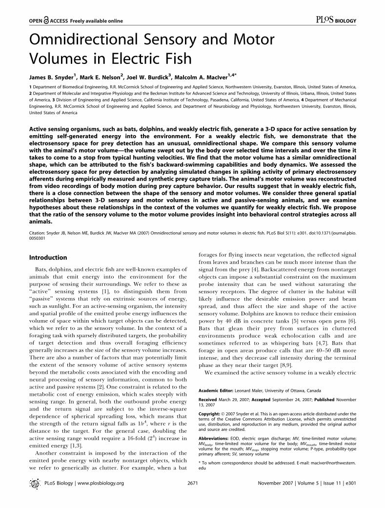
fish, the South American black ghost knifefish (Apteronotusalbifrons), which captures prey in the dark using its activeelectric sense [10,11]. Black ghost knifefish sense theirsurroundings using a weak, self-generated electric field(Figure 1A). Nearby objects that differ in electrical con-ductivity from the surrounding water create localized voltageperturbations across the skin that are sensed by ;14,000electroreceptor organs (Figure 1B). In a previous preycapture study, it was shown that A. albifrons can detect smallprey (Daphnia magna) in the dark at a distance of approx-imately 20–30 mm [11]. The detection points in the earlierstudy were distributed along the entire rostrocaudal axis ofthe fish, primarily in a hemi-cylinder above the dorsal surface(Figure 2). This dorsal bias was, in part, related to themethodology used to introduce prey into the tank in thatstudy. Here, we used computer modeling to simulate preytrajectories that are uniformly distributed, thus allowing us toobtain a more complete and less biased estimate of the 3-Dsensory volume.

The motor capabilities of A. albifrons are as unique as itssensory capabilities. It has a multidirectional propulsionsystem driven primarily by a ribbon fin that runs most of thelength of the body (Figure 3A; interactive 3-D version FigureS1). With this fin, in combination with pectoral fins, the fishcan move forward, backward, upward, and can rapidly pitchor roll the body [11–13].

We will make comparisons between the sensory volume forprey (D. magna) and the motor volume—the locations in spacethat the animal can reach through activation of its muscu-loskeletal system. We will make these terms precise in thefollowing section and pose hypotheses regarding possiblerelationships between sensory and motor volumes in animals.We will then examine these hypotheses in the context ofsensory and motor volumes of electric fish.

Definition of Motor VolumeThe motor volume is the swept volume of positions a body

occupies for a given trajectory or set of trajectories. It is afunction of the way the body moves, as well as the geometricextent of the body. To define it more clearly, we first present

a definition of the time-limited reachable set. We then usethis definition to informally define the motor volume and thestopping motor volume (the swept volume of the body overtrajectories that bring the body to a halt), with the precisedefinitions presented in Text S1.For simplicity of description, we treat an organism as a

rigid 3-D body. We define the configuration space as the six-dimensional space representing the rigid-body degrees offreedom (typically the (x, y, z) position of the center of mass,and h, /, and X, the yaw, pitch, and roll angles, respectively).The state space X consists of the six configuration compo-nents and their time rates of change (vx, vy, vz, vh, v/, vX),resulting in a total of twelve dimensions. The dynamics of thesystem are given by

_x ¼ f ðx; uÞ u 2 U ð1Þ

where x is the instantaneous state and u is the instantaneouscontrol input from the space U of all feasible instantaneouscontrol inputs. The time-limited reachable set R(x0,T) is aconstruct from nonlinear control system theory [14–16]referring to all points in the state space X that can bereached by a system of the form given by Equation 1 from aninitial state x0 given any feasible control history u of durationT. A feasible control history is a control input to the system asa function of time, such as muscle activations for amusculoskeletal system or steering wheel angles for a car.The reachable set is defined as:

Figure 1. Spatial Distributions in the Active Electrosensory System of A.

albifrons

(A) Magnitude of the self-generated electric field in water of 35-lS/cmconductivity from an empirically validated computational model [41]. (B)Density of tuberous (active) electroreceptor sense organs (interpolatedfrom measurements in [44]). The fish is shown without fins because thereare no electroreceptors on the fins.doi:10.1371/journal.pbio.0050301.g001


Omnidirectional Sensory and Motor Volumes

Author Summary

Most animals, including humans, have sensory and motor capa-bilities that are biased in the forward direction. The black ghostknifefish, a nocturnal, weakly electric fish from the Amazon, is aninteresting exception to this general rule. We demonstrate thatthese fish have sensing and motor capabilities that are omnidirec-tional. By combining video analysis of prey capture trajectories withcomputational modeling of the fish’s electrosensory capabilities, wewere able to quantify and compare the 3-D volumes for sensationand movement. We found that the volume in which prey aredetected is similar in size to the volume needed by the fish to stop.We suggest that this coupling may arise from constraints that theanimal faces when using self-generated energy to probe itsenvironment. This is similar to the way in which the angularcoverage and range of an automobile’s headlights are designed tomatch certain motion characteristics of the vehicle, such as itstypical cruising speed, turning angle, and stopping distance. Wesuggest that the degree of overlap between sensory and movementvolumes can provide insight into the types of control strategies thatare best suited for guiding behavior.

Rðx0;TÞ ¼ fx 2 X j 9 feasible u : ½0;T� ! U taking

xð0Þ ¼ x0 to xðTÞ ¼ x by Equation 1g

ð2Þ

This is the set of states reachable in time exactly T. In oursubsequent definitions, we will use the union of all reachablesets from t ¼ 0 to t ¼ T, denoted as:

Rðx0;� TÞ ¼[

t2½0;T�Rðx0; tÞ ð3Þ

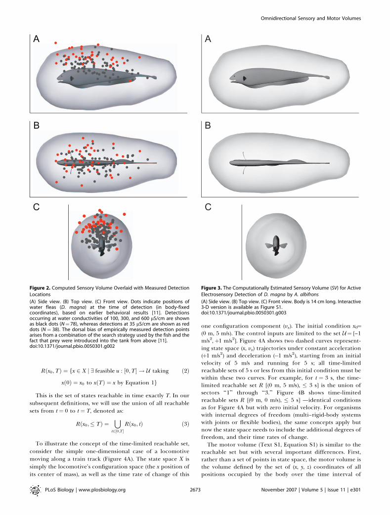
To illustrate the concept of the time-limited reachable set,consider the simple one-dimensional case of a locomotivemoving along a train track (Figure 4A). The state space X issimply the locomotive’s configuration space (the x position ofits center of mass), as well as the time rate of change of this

one configuration component (vx). The initial condition x0¼(0 m, 5 m/s). The control inputs are limited to the set U¼ [–1m/s2,þ1 m/s2]. Figure 4A shows two dashed curves represent-ing state space (x, vx) trajectories under constant acceleration(þ1 m/s2) and deceleration (�1 m/s2), starting from an initialvelocity of 5 m/s and running for 5 s; all time-limitedreachable sets of 5 s or less from this initial condition must bewithin these two curves. For example, for t ¼ 3 s, the time-limited reachable set R [(0 m, 5 m/s), � 3 s] is the union ofsectors ‘‘1’’ through ‘‘3.’’ Figure 4B shows time-limitedreachable sets R [(0 m, 0 m/s), � 5 s] —identical conditionsas for Figure 4A but with zero initial velocity. For organismswith internal degrees of freedom (multi–rigid-body systemswith joints or flexible bodies), the same concepts apply butnow the state space needs to include the additional degrees offreedom, and their time rates of change.The motor volume (Text S1, Equation S1) is similar to the

reachable set but with several important differences. First,rather than a set of points in state space, the motor volume isthe volume defined by the set of (x, y, z) coordinates of allpositions occupied by the body over the time interval of

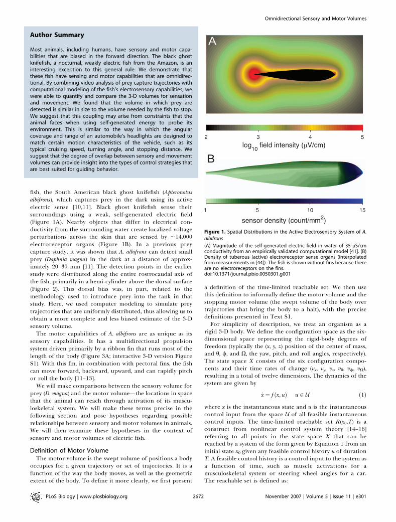
Figure 3. The Computationally Estimated Sensory Volume (SV) for Active

Electrosensory Detection of D. magna by A. albifrons

(A) Side view. (B) Top view. (C) Front view. Body is 14 cm long. Interactive3-D version is available as Figure S1.doi:10.1371/journal.pbio.0050301.g003

Figure 2. Computed Sensory Volume Overlaid with Measured Detection

Locations

(A) Side view. (B) Top view. (C) Front view. Dots indicate positions ofwater fleas (D. magna) at the time of detection (in body-fixedcoordinates), based on earlier behavioral results [11]. Detectionsoccurring at water conductivities of 100, 300, and 600 lS/cm are shownas black dots (N¼ 78), whereas detections at 35 lS/cm are shown as reddots (N ¼ 38). The dorsal bias of empirically measured detection pointsarises from a combination of the search strategy used by the fish and thefact that prey were introduced into the tank from above [11].doi:10.1371/journal.pbio.0050301.g002



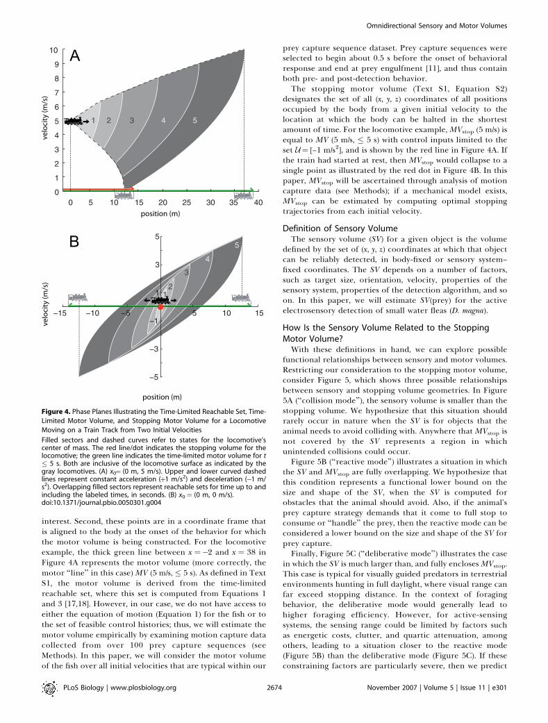
interest. Second, these points are in a coordinate frame thatis aligned to the body at the onset of the behavior for whichthe motor volume is being constructed. For the locomotiveexample, the thick green line between x ¼�2 and x ¼ 38 inFigure 4A represents the motor volume (more correctly, themotor ‘‘line’’ in this case)MV (5 m/s, � 5 s). As defined in TextS1, the motor volume is derived from the time-limitedreachable set, where this set is computed from Equations 1and 3 [17,18]. However, in our case, we do not have access toeither the equation of motion (Equation 1) for the fish or tothe set of feasible control histories; thus, we will estimate themotor volume empirically by examining motion capture datacollected from over 100 prey capture sequences (seeMethods). In this paper, we will consider the motor volumeof the fish over all initial velocities that are typical within our

prey capture sequence dataset. Prey capture sequences wereselected to begin about 0.5 s before the onset of behavioralresponse and end at prey engulfment [11], and thus containboth pre- and post-detection behavior.The stopping motor volume (Text S1, Equation S2)

designates the set of all (x, y, z) coordinates of all positionsoccupied by the body from a given initial velocity to thelocation at which the body can be halted in the shortestamount of time. For the locomotive example, MVstop (5 m/s) isequal to MV (5 m/s, � 5 s) with control inputs limited to theset U¼ [–1 m/s2], and is shown by the red line in Figure 4A. Ifthe train had started at rest, then MVstop would collapse to asingle point as illustrated by the red dot in Figure 4B. In thispaper, MVstop will be ascertained through analysis of motioncapture data (see Methods); if a mechanical model exists,MVstop can be estimated by computing optimal stoppingtrajectories from each initial velocity.

Definition of Sensory VolumeThe sensory volume (SV) for a given object is the volume

defined by the set of (x, y, z) coordinates at which that objectcan be reliably detected, in body-fixed or sensory system–fixed coordinates. The SV depends on a number of factors,such as target size, orientation, velocity, properties of thesensory system, properties of the detection algorithm, and soon. In this paper, we will estimate SV(prey) for the activeelectrosensory detection of small water fleas (D. magna).

How Is the Sensory Volume Related to the StoppingMotor Volume?With these definitions in hand, we can explore possible

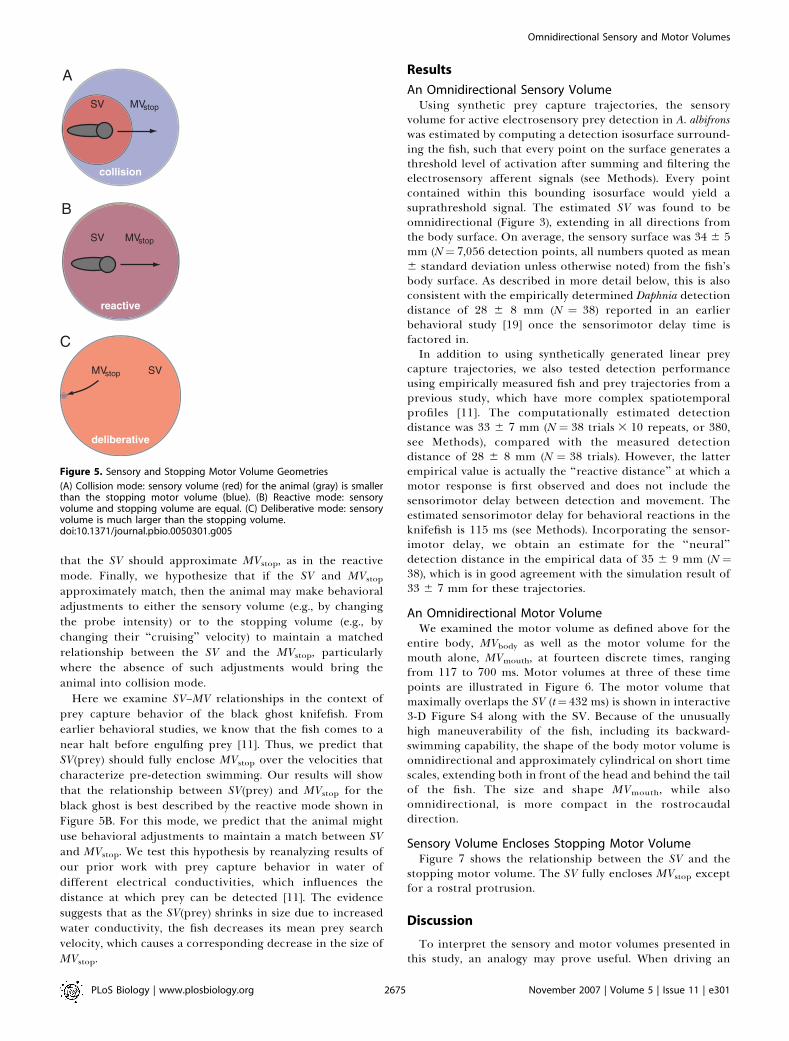
functional relationships between sensory and motor volumes.Restricting our consideration to the stopping motor volume,consider Figure 5, which shows three possible relationshipsbetween sensory and stopping volume geometries. In Figure5A (‘‘collision mode’’), the sensory volume is smaller than thestopping volume. We hypothesize that this situation shouldrarely occur in nature when the SV is for objects that theanimal needs to avoid colliding with. Anywhere that MVstop isnot covered by the SV represents a region in whichunintended collisions could occur.Figure 5B (‘‘reactive mode’’) illustrates a situation in which

the SV and MVstop are fully overlapping. We hypothesize thatthis condition represents a functional lower bound on thesize and shape of the SV, when the SV is computed forobstacles that the animal should avoid. Also, if the animal’sprey capture strategy demands that it come to full stop toconsume or ‘‘handle’’ the prey, then the reactive mode can beconsidered a lower bound on the size and shape of the SV forprey capture.Finally, Figure 5C (‘‘deliberative mode’’) illustrates the case

in which the SV is much larger than, and fully enclosesMVstop.This case is typical for visually guided predators in terrestrialenvironments hunting in full daylight, where visual range canfar exceed stopping distance. In the context of foragingbehavior, the deliberative mode would generally lead tohigher foraging efficiency. However, for active-sensingsystems, the sensing range could be limited by factors suchas energetic costs, clutter, and quartic attenuation, amongothers, leading to a situation closer to the reactive mode(Figure 5B) than the deliberative mode (Figure 5C). If theseconstraining factors are particularly severe, then we predict

Figure 4. Phase Planes Illustrating the Time-Limited Reachable Set, Time-

Limited Motor Volume, and Stopping Motor Volume for a Locomotive

Moving on a Train Track from Two Initial Velocities

Filled sectors and dashed curves refer to states for the locomotive’scenter of mass. The red line/dot indicates the stopping volume for thelocomotive; the green line indicates the time-limited motor volume for t� 5 s. Both are inclusive of the locomotive surface as indicated by thegray locomotives. (A) x0¼ (0 m, 5 m/s). Upper and lower curved dashedlines represent constant acceleration (þ1 m/s2) and deceleration (�1 m/s2). Overlapping filled sectors represent reachable sets for time up to andincluding the labeled times, in seconds. (B) x0¼ (0 m, 0 m/s).doi:10.1371/journal.pbio.0050301.g004



that the SV should approximate MVstop, as in the reactivemode. Finally, we hypothesize that if the SV and MVstop

approximately match, then the animal may make behavioraladjustments to either the sensory volume (e.g., by changingthe probe intensity) or to the stopping volume (e.g., bychanging their ‘‘cruising’’ velocity) to maintain a matchedrelationship between the SV and the MVstop, particularlywhere the absence of such adjustments would bring theanimal into collision mode.

Here we examine SV–MV relationships in the context ofprey capture behavior of the black ghost knifefish. Fromearlier behavioral studies, we know that the fish comes to anear halt before engulfing prey [11]. Thus, we predict thatSV(prey) should fully enclose MVstop over the velocities thatcharacterize pre-detection swimming. Our results will showthat the relationship between SV(prey) and MVstop for theblack ghost is best described by the reactive mode shown inFigure 5B. For this mode, we predict that the animal mightuse behavioral adjustments to maintain a match between SVand MVstop. We test this hypothesis by reanalyzing results ofour prior work with prey capture behavior in water ofdifferent electrical conductivities, which influences thedistance at which prey can be detected [11]. The evidencesuggests that as the SV(prey) shrinks in size due to increasedwater conductivity, the fish decreases its mean prey searchvelocity, which causes a corresponding decrease in the size ofMVstop.

Results

An Omnidirectional Sensory VolumeUsing synthetic prey capture trajectories, the sensory

volume for active electrosensory prey detection in A. albifronswas estimated by computing a detection isosurface surround-ing the fish, such that every point on the surface generates athreshold level of activation after summing and filtering theelectrosensory afferent signals (see Methods). Every pointcontained within this bounding isosurface would yield asuprathreshold signal. The estimated SV was found to beomnidirectional (Figure 3), extending in all directions fromthe body surface. On average, the sensory surface was 34 6 5mm (N¼ 7,056 detection points, all numbers quoted as mean6 standard deviation unless otherwise noted) from the fish’sbody surface. As described in more detail below, this is alsoconsistent with the empirically determined Daphnia detectiondistance of 28 6 8 mm (N ¼ 38) reported in an earlierbehavioral study [19] once the sensorimotor delay time isfactored in.In addition to using synthetically generated linear prey

capture trajectories, we also tested detection performanceusing empirically measured fish and prey trajectories from aprevious study, which have more complex spatiotemporalprofiles [11]. The computationally estimated detectiondistance was 33 6 7 mm (N ¼ 38 trials 3 10 repeats, or 380,see Methods), compared with the measured detectiondistance of 28 6 8 mm (N ¼ 38 trials). However, the latterempirical value is actually the ‘‘reactive distance’’ at which amotor response is first observed and does not include thesensorimotor delay between detection and movement. Theestimated sensorimotor delay for behavioral reactions in theknifefish is 115 ms (see Methods). Incorporating the sensor-imotor delay, we obtain an estimate for the ‘‘neural’’detection distance in the empirical data of 35 6 9 mm (N ¼38), which is in good agreement with the simulation result of33 6 7 mm for these trajectories.

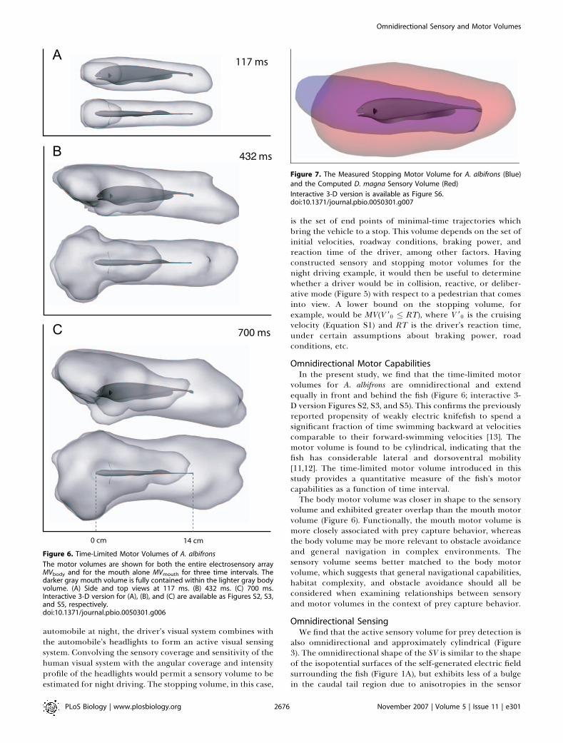
An Omnidirectional Motor VolumeWe examined the motor volume as defined above for the

entire body, MVbody as well as the motor volume for themouth alone, MVmouth, at fourteen discrete times, rangingfrom 117 to 700 ms. Motor volumes at three of these timepoints are illustrated in Figure 6. The motor volume thatmaximally overlaps the SV (t¼ 432 ms) is shown in interactive3-D Figure S4 along with the SV. Because of the unusuallyhigh maneuverability of the fish, including its backward-swimming capability, the shape of the body motor volume isomnidirectional and approximately cylindrical on short timescales, extending both in front of the head and behind the tailof the fish. The size and shape MVmouth, while alsoomnidirectional, is more compact in the rostrocaudaldirection.

Sensory Volume Encloses Stopping Motor VolumeFigure 7 shows the relationship between the SV and the

stopping motor volume. The SV fully encloses MVstop exceptfor a rostral protrusion.

Discussion

To interpret the sensory and motor volumes presented inthis study, an analogy may prove useful. When driving an

Figure 5. Sensory and Stopping Motor Volume Geometries

(A) Collision mode: sensory volume (red) for the animal (gray) is smallerthan the stopping motor volume (blue). (B) Reactive mode: sensoryvolume and stopping volume are equal. (C) Deliberative mode: sensoryvolume is much larger than the stopping volume.doi:10.1371/journal.pbio.0050301.g005



automobile at night, the driver’s visual system combines withthe automobile’s headlights to form an active visual sensingsystem. Convolving the sensory coverage and sensitivity of thehuman visual system with the angular coverage and intensityprofile of the headlights would permit a sensory volume to beestimated for night driving. The stopping volume, in this case,

is the set of end points of minimal-time trajectories whichbring the vehicle to a stop. This volume depends on the set ofinitial velocities, roadway conditions, braking power, andreaction time of the driver, among other factors. Havingconstructed sensory and stopping motor volumes for thenight driving example, it would then be useful to determinewhether a driver would be in collision, reactive, or deliber-ative mode (Figure 5) with respect to a pedestrian that comesinto view. A lower bound on the stopping volume, forexample, would be MV(V 90 � RT), where V 90 is the cruisingvelocity (Equation S1) and RT is the driver’s reaction time,under certain assumptions about braking power, roadconditions, etc.

Omnidirectional Motor CapabilitiesIn the present study, we find that the time-limited motor

volumes for A. albifrons are omnidirectional and extendequally in front and behind the fish (Figure 6; interactive 3-D version Figures S2, S3, and S5). This confirms the previouslyreported propensity of weakly electric knifefish to spend asignificant fraction of time swimming backward at velocitiescomparable to their forward-swimming velocities [13]. Themotor volume is found to be cylindrical, indicating that thefish has considerable lateral and dorsoventral mobility[11,12]. The time-limited motor volume introduced in thisstudy provides a quantitative measure of the fish’s motorcapabilities as a function of time interval.The body motor volume was closer in shape to the sensory

volume and exhibited greater overlap than the mouth motorvolume (Figure 6). Functionally, the mouth motor volume ismore closely associated with prey capture behavior, whereasthe body volume may be more relevant to obstacle avoidanceand general navigation in complex environments. Thesensory volume seems better matched to the body motorvolume, which suggests that general navigational capabilities,habitat complexity, and obstacle avoidance should all beconsidered when examining relationships between sensoryand motor volumes in the context of prey capture behavior.

Omnidirectional SensingWe find that the active sensory volume for prey detection is

also omnidirectional and approximately cylindrical (Figure3). The omnidirectional shape of the SV is similar to the shapeof the isopotential surfaces of the self-generated electric fieldsurrounding the fish (Figure 1A), but exhibits less of a bulgein the caudal tail region due to anisotropies in the sensor

Figure 6. Time-Limited Motor Volumes of A. albifrons

The motor volumes are shown for both the entire electrosensory arrayMVbody and for the mouth alone MVmouth for three time intervals. Thedarker gray mouth volume is fully contained within the lighter gray bodyvolume. (A) Side and top views at 117 ms. (B) 432 ms. (C) 700 ms.Interactive 3-D version for (A), (B), and (C) are available as Figures S2, S3,and S5, respectively.doi:10.1371/journal.pbio.0050301.g006

Figure 7. The Measured Stopping Motor Volume for A. albifrons (Blue)

and the Computed D. magna Sensory Volume (Red)

Interactive 3-D version is available as Figure S6.doi:10.1371/journal.pbio.0050301.g007



density (Figure 1B), field intensity (Figure 1A), reducedsensory surface area due to the tapering body morphology(Figure 1B), and the sensitivity of the primary electrosensoryafferents to prey-induced perturbations [20,21]. The relativeimportance of these factors in determining the precise shapeof the sensory volume was not examined. It will beparticularly interesting in future studies to explore the extentto which the higher electroreceptor density in the headregion of the fish influences prey-detection distance versusspatial resolution of prey position. The simulations of preydetection in this study combined quantitative models of eachof these factors in order to arrive at an estimated sensoryvolume for electrosensory-mediated prey detection. As shownin Figure 2, there was good agreement between the computa-tionally estimated sensory volume and the empirical distri-bution of prey detections found in an earlier study [11]. Theempirical study had relatively low N (38 prey capture eventsfor the water conductivity that yielded maximum detectionrange), and the detection points were biased toward thedorsal surface of the fish, because prey were introduced intothe tank from above. The computational approach used hereallowed us to obtain a more complete and less biased estimateof the fish’s sensory detection volume.

Enclosure of the Stopping Motor Volume by the SensoryVolume

Our prediction that the fish avoids collision mode issupported by Figure 7 (interactive 3-D version Figure S6),which shows nearly full enclosure of the stopping volume bythe sensory volume. The stopping volume was taken from justbefore detection (which always occurred during forwardmovement) to the point of zero forward velocity as the fishreverses to capture the prey. Thus, unlike the time-limitedmotor volume, which sampled all initial velocities includingnegative velocities, the stopping volume is more stronglybiased in the forward direction.

However, the extent of the sensing range is restricted tonearly the lower limit of the reactive mode (Figure 5B) wherethe SV and MV are matched. We expect this is due toconstraints that include the metabolic cost for emittingenergy into the environment and the interference caused byinteraction between the emitted signal and nearby clutter.Energetic costs scale steeply with sensing range, approx-imately as a quartic power of the range due to geometricspreading effects on the outbound and return paths of activeprobe signal [1,3]. For quartic scaling, doubling the active-sensing range would require a 16-fold increase in emittedenergy. To appreciate the effect of this scaling, consider thatan active 15-g A. albifrons requires approximately 300 J/day[22]. If we assume that ’1% is used for the field, as estimatedfor another weakly electric fish [23], then 3 J/day is needed forthe field. To double the detection distance for D. magna fromthe measured ’30 mm to ’60 mm would therefore require48 J/day for the field; to double this again to ’120 mm (stillless than one body length for a 15-g fish) would then require768 J/day, more than double the entire energy budget of thefish. Thus, the high energetic costs associated with extendingthe active-sensing range is likely to place strong selectivepressure on the shape and extent of the active sensoryvolume. In comparison, the high acuity passive visual systemof a typical raptor allows it to spot prey from over a kilometeraway, or about 10,000 body lengths.

Although it is more difficult to provide a quantitativemetric for the interference effects from clutter, the greatreduction in emission power observed in dolphins and batswhen surrounded by clutter or when nearing a target (seeIntroduction) suggests that this may also be an importantfactor in limiting the desirable range of an emitted signal.Returning to the automobile scenario, driving at night in adense fog provides a practical example of where backscatteris a limiting constraint. Increasing headlight intensity underthese conditions (e.g., switching from low beams to highbeams) can actually degrade detection performance becausethe ‘‘noise’’ from backscattered light makes it more difficultto detect the ‘‘signal’’ that is reflected back from a target ofinterest.Given that the black ghost is in reactive mode, we predict

that the fish may make behavioral adjustments to either thesensory volume or to the stopping volume to maintain amatched relationship between the SV and the MVstop,particularly where the absence of such adjustments wouldbring the animal into collision mode. We are able toqualitatively evaluate this hypothesis by examining howsearch (predetection) swimming velocity varies with waterconductivity. We have shown that water conductivity changesthe range at which prey are detected [11]. In the previousstudy [11], we found that the mean detection distancedecreased from 28 mm at a water conductivity of 35 lS/cmto 12 mm at 600 lS/cm. Over this conductivity range, the fish’spredetection swimming velocity decreased 30% from 99 mm/sto 71 mm/s. At the shorter detection distances associated withhigher conductivity water (600 lS/cm), we have previouslyestimated that multiple sensory modalities, including passiveelectrosense and lateral line mechanosense, are playing a role[24]. Thus, quantitative evaluation of the matching hypothesiswould require modeling the SV for these other sensorymodalities, which is outside the scope of this study.

Neural ImplicationsThe size of the estimated sensory volume, and to a lesser

degree the shape of the volume, are influenced by theproperties of the neural detection algorithm. A moresensitive algorithm will result in a larger detection range.The detection algorithm used here is not intended to modelthe fish’s actual detection performance in detail. Doing sowould require a more extensive analysis of additional factors,such as sensory reafference associated with tail bending,environmental background noise, contributions of othersensory modalities, neuroanatomical constraints on sensoryconvergence, etc. Rather, the detection volume reconstructedhere is intended as an estimate of ‘‘best-case’’ detectionperformance based solely on changes in active electrosensoryafferent spike activity.

Comparison with Other Active-sensing SpeciesEcholocating bats emit ultrasonic energy into the environ-

ment to detect prey [25]. While the precise size and shape ofthe bat’s sensory volume will vary with many factors (species,call intensity, duration, etc.), the sensory volume forecholocation is generally a cone that extends in front of thehead of the bat with an angular range of approximately 6308

in azimuth and elevation [26]. The angular coverage mayextend as much as 6758 relative to the body axis when headand pinnae movements are included [25,27,28]. For the



detection of flying insects by pipistrelle bats, the sensoryvolume extends at least 100–200 cm in front of the animal[25,29] based on the reactive distance to prey.

The detailed shape of the bat’s motor volume has not beenreported. The stopping distance can be estimated bycombining information on the initial velocity of the bat,maximal deceleration, and sensorimotor time delay. Taking arepresentative bat cruising velocity of 5 m/s [25], a maximaldeceleration of 15 m/s2 (estimated from a sample trajectory in[25]), and an estimated sensorimotor delay of 100–200 ms [30]yields an estimated stopping distance in the range of 130–180cm. Although there is a great deal of uncertainty in theseestimates, the stopping distance of the bat seems comparableto the sensory range for prey detection. This suggests thatbats, like electric fish, have an active sensory volume for preydetection that may be comparable to their stopping volume.Quantitative comparisons of sensory and motor volumes for asingle bat species would help clarify these relationships.

Odontocetes (toothed whales, dolphins, and porpoises) alsouse ultrasonic energy for prey detection. Dolphins can detectprey-sized objects at distances on the order of 100 m [6,31].The 100-m sensing range of dolphins is certain to besignificantly beyond their stopping volume, although thereis little published data with which to make quantitative

comparisons. This suggests that energetic and clutter-relatedconstraints on active sensing may not be as significant fordolphins as they are for bats and electric fish.

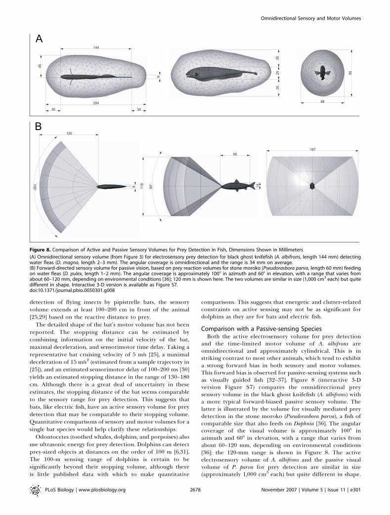
Comparison with a Passive-sensing SpeciesBoth the active electrosensory volume for prey detection

and the time-limited motor volume of A. albifrons areomnidirectional and approximately cylindrical. This is instriking contrast to most other animals, which tend to exhibita strong forward bias in both sensory and motor volumes.This forward bias is observed for passive-sensing systems suchas visually guided fish [32–37]. Figure 8 (interactive 3-Dversion Figure S7) compares the omnidirectional preysensory volume in the black ghost knifefish (A. albifrons) witha more typical forward-biased passive sensory volume. Thelatter is illustrated by the volume for visually mediated preydetection in the stone moroko (Pseudorasbora parva), a fish ofcomparable size that also feeds on Daphnia [36]. The angularcoverage of the visual volume is approximately 1008 inazimuth and 608 in elevation, with a range that varies fromabout 60–120 mm, depending on environmental conditions[36]; the 120-mm range is shown in Figure 8. The activeelectrosensory volume of A. albifrons and the passive visualvolume of P. parva for prey detection are similar in size(approximately 1,000 cm3 each) but quite different in shape.

45

88

9525

35

144

30

204

35

187

120

100° 11

9

60°

60

8 14

30

9

Figure 8. Comparison of Active and Passive Sensory Volumes for Prey Detection in Fish, Dimensions Shown in Millimeters

(A) Omnidirectional sensory volume (from Figure 3) for electrosensory prey detection for black ghost knifefish (A. albifrons, length 144 mm) detectingwater fleas (D. magna, length 2–3 mm). The angular coverage is omnidirectional and the range is 34 mm on average.(B) Forward-directed sensory volume for passive vision, based on prey reaction volumes for stone moroko (Pseudorasbora parva, length 60 mm) feedingon water fleas (D. pulex, length 1–2 mm). The angular coverage is approximately 1008 in azimuth and 608 in elevation, with a range that varies fromabout 60–120 mm, depending on environmental conditions [36]; 120 mm is shown here. The two volumes are similar in size (1,000 cm3 each) but quitedifferent in shape. Interactive 3-D version is available as Figure S7.doi:10.1371/journal.pbio.0050301.g008



A New Metric for Control System AnalysisWe propose that the ratio of the sensory volume to

stopping volume (SV:MVstop) is a useful metric for both activeand passive sensory systems when considering whethersensorimotor control systems are in collision, reactive, ordeliberative mode. Collision mode occurs when the ratio isbelow unity. Reactive mode occurs when the ratio approx-imates unity, as appears to be the case for knifefish and bats.In this mode, sensorimotor control algorithms are likely to bereactive, with relatively fast, direct coupling between sensa-tion and action. Movement options are largely conditioned bymechanical considerations such as inertia and minimalturning radius. For example, some sensor-based motionplanning algorithms in robotics are based on estimating thestopping volume for the nearest obstacle; as the robotbecomes more massive, the range of any active-sensing systemfor obstacle detection must be extended accordingly [38].Deliberative mode occurs when the ratio is large, as fordolphin echolocation and for many passive visual andauditory systems. In this mode, an animal can acquire sensorydata from targets that are far outside its stopping volume.This allows the animal a greater range of movement options,because there is adequate time for complex motion planningbefore reaching the target [39]. For example, in the context ofprey capture behavior, a dolphin with a high SV:MVstop ratiois able to engage in long-range tracking of distant prey,whereas a weakly electric fish with a ratio near unity must usea reactive strategy for chance encounters with nearby prey.Quantitative analyses of sensory and motor volumes for bothactive and passive-sensing systems can highlight importantfunctional relationships between sensing, movement, andbehavioral control in animals.

Materials and Methods

Behavioral data. In a previously published study [11], adult weaklyelectric fish (A. albifrons) were videotaped in a light-tight enclosureunder infrared illumination. Individual water fleas (D. magna, 2–3 mm

in length) were introduced near the water surface and drifteddownward; prey capture behavior was recorded using a pair of videocameras oriented along orthogonal axes. Relative to the fish’s velocity(;100 mm/s) the prey were relatively stationary (prey velocity , 20mm/s). Prey capture events (from shortly before detection to capture)were subsequently digitized, and 3-D motion trajectories of the fishsurface and prey were obtained using a model-based tracking systemwith a spatial resolution of 0.5 mm and a temporal resolution of 1/60 s[40]. The time of prey detection was defined by the onset of an abruptlongitudinal deceleration as the fish reversed swimming direction tocapture the prey [11]. These reversals are characteristic of most preycapture encounters. This is related to the fact that the fish tends toswim forward with its head pitched downward, such that the dorsumforms the leading edge as the fish moves through the water. Initialprey encounters thus tend to be uniformly distributed along theentire length of the body, so a reversal of swimming direction istypically required to intercept the prey.

Sensory volume (SV) for electrosensory prey detection. The volumeof space supporting prey detection by the active electric sense wasestimated computationally using measurements and empiricallyconstrained models of the prey, electric field, fish body and sensordistribution, electrosensory images, afferent firing dynamics, andbehavior. Model parameter values and their sources are summarizedin Table 1.

Electric field. The electric field vector Efish (mV/cm) at a 3-D point inspace x was computed using an empirically tested model of theelectric field [41]. This model sums the individual contributions tothe field from each of a series of charged poles used to model theelectric organ of the fish:

EfishðxÞ ¼Xmi¼1

q=m

jx� xipj3x� xip� �

�Xni¼mþ1

q=ðn� mÞjx� xipj3

x� xip� �" #

rmes

rmod

ð4Þ

where x is a point in space (cm), xip is the location of pole i of n totalpoles, q is a normalization constant (mV cm) that scales the overallmagnitude of the field, rmes is the conductivity of the water that thefield measurements were performed in (which establishes the qvalue), and rmod is the conductivity of the water for the simulatedfield. The quantity q is analogous to electric charge in an electro-static model and is distributed such that the first m poles have a‘‘charge’’ of q/m and the remaining poles have a charge of –q/(n – m),resulting in a total net charge of zero. For our simulations, n¼ 267, m¼ 266 (all but one pole at the tail was positive), q ¼ 10, and the polelocations xp ran from the nose to the tail of the fish along the centralaxis of the fish body with equidistant spacing. These values resultedin field values within 10% of measurements of the electric field

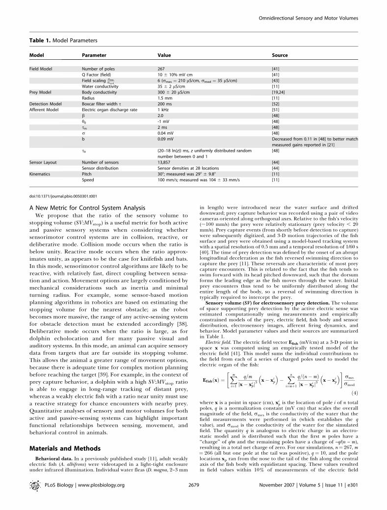
Table 1. Model Parameters

Model Parameter Value Source

Field Model Number of poles 267 [41]

Q Factor (field) 10 6 10% mV cm [41]

Field scaling rmes

rmod6 (rmes ¼ 210 lS/cm, rmod ¼ 35 lS/cm) [43]

Water conductivity 35 6 2 lS/cm [11]

Prey Model Body conductivity 300 6 20 lS/cm [19,24]

Radius 1.5 mm [11]

Detection Model Boxcar filter width s 200 ms [52]

Afferent Model Electric organ discharge rate 1 kHz [51]

b 2.0 [48]

h0 -1 mV [48]

sm 2 ms [48]

r 0.04 mV [48]

b 0.09 mV Decreased from 0.11 in [48] to better match

measured gains reported in [21]

sh (20–18 ln(z)) ms, z uniformly distributed random

number between 0 and 1

[48]

Sensor Layout Number of sensors 13,857 [44]

Sensor distribution Sensor densities at 28 locations [44]

Kinematics Pitch 308; measured was 298 6 9.88 [11]

Speed 100 mm/s; measured was 104 6 33 mm/s [11]

doi:10.1371/journal.pbio.0050301.t001



vector Efish of A. albifrons obtained by other researchers (B. Rasnow,C. Assad, P. Stoddard, unpublished data) in water of conductivityrmes ¼ 210 lS/cm using a multiaxis electrode array [20,42] (Figure1A). The rmes

rmodterm scales the field strength to the water conductivity

used in simulation rmod ¼ 35 lS/cm. This scaling is based onempirical measurements of the knifefish field at different waterconductivities [43], which suggest the electric organ can be idealizedas constant current source. We selected 35 lS/cm because our earlierstudy [11] found that the detection range was highest for trials at thisconductivity, and this conductivity is most similar to rivers of thefish’s native habitat.

Body model with electroreceptor distribution. We used a prior survey [44]of the density of probability type (P-type) tuberous electroreceptororgans (hereafter electroreceptors) on the surface of A. albifrons.These are the dominant electroreceptor type for A. albifrons [45,46].Each electroreceptor is connected uniquely to a primary afferent,which generates action potentials with a probability that varies withstimulus intensity. The receptor locations were mapped onto a high-resolution polygonal model of the fish derived from a 3-D scan of abody cast [19,24] in accordance with the measured sensor densities[44] (Figure 1B). This resulted in a total of 13,857 mapped electro-receptors, in close agreement with neuroanatomically derived countsfrom A. albifrons [44].

Prey model. Based on prior measurements of live prey (D. magna), itwas modeled as a 1.5-mm-radius conductive sphere with an electricalconductance of robj ¼ 300 lS/cm [19,24]. Idealizing the prey as asphere allows us to use an analytical model for the stimulus caused bythe prey, described below.

Electrosensory image formation. The voltage perturbation D/ (mV) atan electroreceptor on the fish surface, arising from a small sphericaltarget object, was computed using an empirically tested model [47]:

D/ðrÞ ¼ a3Efish�rr3

robj � rw

robj þ 2rw

� �� ð5Þ

where Efish (mV/cm) is the electric field vector at the prey, r (cm) is thevector from the center of the spherical object to the electroreceptoron the fish surface, a is the radius of the sphere (cm), robj is theconductivity of the sphere, and rw is the conductivity of the water(lS/cm). Simulations were run with water conductivity rw set to 35 lS/cm (see Methods, Electric field).

Primary afferent spiking activity. Computed voltage perturbations ateach sensory receptor on the fish body were transformed intoprimary afferent spiking activity using a previously publishedadaptive threshold model of P-type (probability coding) primaryelectrosensory afferent response dynamics [48]. This model gives riseto negative correlations in the interspike interval (ISI) sequence,which lead to long-term spike train regularization. This correlationstructure has been shown to increase information transfer andimprove detection performance for weak signals [48–50]. The electricorgan discharge (EOD) frequency was taken as 1 kHz, which is typicalof A. albifrons [51]. P-type afferents fire at most one spike per EODcycle. Thus, afferent activity was modeled as a binary spike train witha sampling period equal to the EOD period (1 ms). On each EODcycle (n), the following update rules are evaluated in order:

u½n� ¼ expð�1=smÞu½n� 1� þ ½1� expð�1=smÞ�bD/½n� ð6Þ

v½n� ¼ u½n� þ w½n� ð7Þ

h½n� ¼ expð�1=shÞh½n� 1� þ ½1� expð�1=shÞ�h0 ð8Þ

s½n� ¼ Hðv½n� � h½n�Þ ¼ 1 if v½n� � h½n�0 otherwise

�ð9Þ

h½n� ¼ h½n� þ bs½n� ¼ h½n� þ b if s½n� ¼ 1h½n� otherwise

�ð10Þ

Equation 6 implements low-pass filtering of the voltage perturba-tion D/[n] with gain b and time constant sm. The state variable u[n]can be conceptualized as a membrane potential; it is initialized to 0,corresponding to the steady-state value with no stimulus present (D/¼ 0). Equation 7 adds random noise to u[n] to create a noisymembrane potential v[n]; the noise w[n] is modeled as zero-meanGaussian noise with variance r2. The actual noise distribution is likelyto be more complex, but the Gaussian approximation adequatelycaptures available empirical data. Equation 8 describes the behaviorof an adaptive spike threshold h[n] that decays toward a baselinethreshold h0 with a time constant sh. Equation 9 represents theprocess of spike generation, where s[n] is the binary spike output (s¼1, spike; s¼ 0, no spike); H is the Heaviside function, defined as H(x)¼0 for x , 0 and H(x)¼ 1 for x � 0. A spike is generated whenever thenoisy membrane potential v[n] exceeds the threshold h[n]. Equation10 implements a relative refractory period by elevating the thresholdh[n] by an amount b immediately following a spike. (The thresholdlevel subsequently decays toward its steady state value according toEquation 8.)

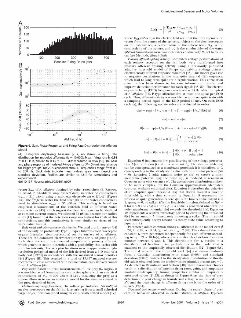
Parameter values common among all afferents in the model were b¼2.0, b¼0.09, r¼0.04, h0¼�1, and sm¼2 [48]. The values of the timeconstant sh were generated independently for each afferent accord-ing to sh ¼ 21 – 18 ln(z), where z is a uniformly-distributed randomnumber between 0 and 1. This distribution for sh results in adistribution of baseline firing probabilities in the model that ismatched to the empirically observed distribution [52] (Figure 9A).The initial value for the threshold level h[n] was drawn randomlyfrom a Gaussian distribution with mean (0.064) and standarddeviation (0.045) matched to the steady-state distribution of thresh-old values obtained from the model with no stimulus present (D/¼0).As detailed in Brandman and Nelson [48], these parameter choicesresult in a distribution of baseline firing rates, gains, and amplitudemodulation–frequency tuning properties similar to empiricallymeasured values [21,53], as shown in Figure 9. At the time of preydetection, the peak change in transdermal voltage is on the order of 1lV, and the peak change in afferent firing rate is on the order of 1spike/s [12,54].

Simulated prey encounter trajectories. During the search phase of preycapture behavior observed in earlier studies, A. albifrons typically

Figure 9. Gain, Phase Response, and Firing Rate Distribution for Afferent

Model

(A) Histogram displaying baseline (2 s, no stimulus) firing ratedistribution for modeled afferents (N ¼ 10,000). Mean firing rate is 0.346 0.11 kHz, similar to 0.33 6 0.13 kHz measured in vivo [53]. (B) Gainand phase response of modeled P-type afferents (N¼5) (minimal changefor larger groups) for 20-s sinusoidal stimuli. Frequencies range from 0.1to 200 Hz. Black dots indicate mean values, gray areas depict onestandard deviation. Profiles are similar to [21] for simulations andexperimental.doi:10.1371/journal.pbio.0050301.g009



swims forward with a mean longitudinal velocity of ;100 mm/s, withits head pitched downward at an angle of ;308 relative to horizontal[11]. The slowly moving prey were relatively stationary, with typicalvelocities less than ;20 mm/s [11]. In the current simulation study, wemodeled this relative motion between the fish and prey by moving theprey target along horizontal rays at 100 mm/s toward a stationarymodel fish pitched downward at 308 (Figure 10A). Two sets of suchprey trajectories were simulated, one set consisting of trajectoriesfrom head-to-tail, the other set from tail-to-head, since the fish swimsforward and backward. A static model of the fish (140 mm long) wascentered within a rectangular box at a pitch of 308. The box size waschosen such that any prey trajectory originating on a box face wouldbegin well outside the detection range of the fish. The shortestdistance between a point on any face of the box and any point on thefish was 60 mm. This distance was set by examining preliminarysimulations and empirical measurements, which showed typicaldetection distances of 20–40 mm. The resulting dimension of thebox was 245 mm (length), 129 mm (width), and 193 mm (height). Forthe head-to-tail trajectories, horizontal prey positions from the frontplane to the back plane were generated with starting and endingpoints centered on a grid with spacing of 5 mm (a total of 1,014trajectories). Variation in starting and ending points was achieved by

adding random values ranging from negative to positive one-half thegrid spacing. Intervening points on the trajectory were on a straightline, at a time interval of 1/60th of a second. The same number of tail-to-head trajectories were generated in the same manner.

Estimating the locations of prey detection from spike train activity.For each simulated trajectory, we use a detection algorithm toestimate the point at which the prey should have become detectablebased on changes in afferent spike activity. The detection points thatemerge from this analysis are then used to estimate the size and shapeof the electrosensory prey detection volume. The approach used hereis not intended to model the fish’s actual detection performance indetail. Doing so would require a more extensive analysis of additionalfactors, such as sensory reafference associated with tail bending,environmental background noise, contributions of other sensorymodalities, neuroanatomical constraints on sensory convergence, etc.Rather, the detection volume reconstructed here is intended as anestimate of ‘‘best-case’’ detection performance, based solely onchanges in electrosensory afferent spike activity.

The voltage perturbation corresponding to each prey position wascomputed from Equation 5 across the full complement of 13,857sensory receptors. The resulting history of voltage perturbations ateach receptor was interpolated to produce values at each millisecond

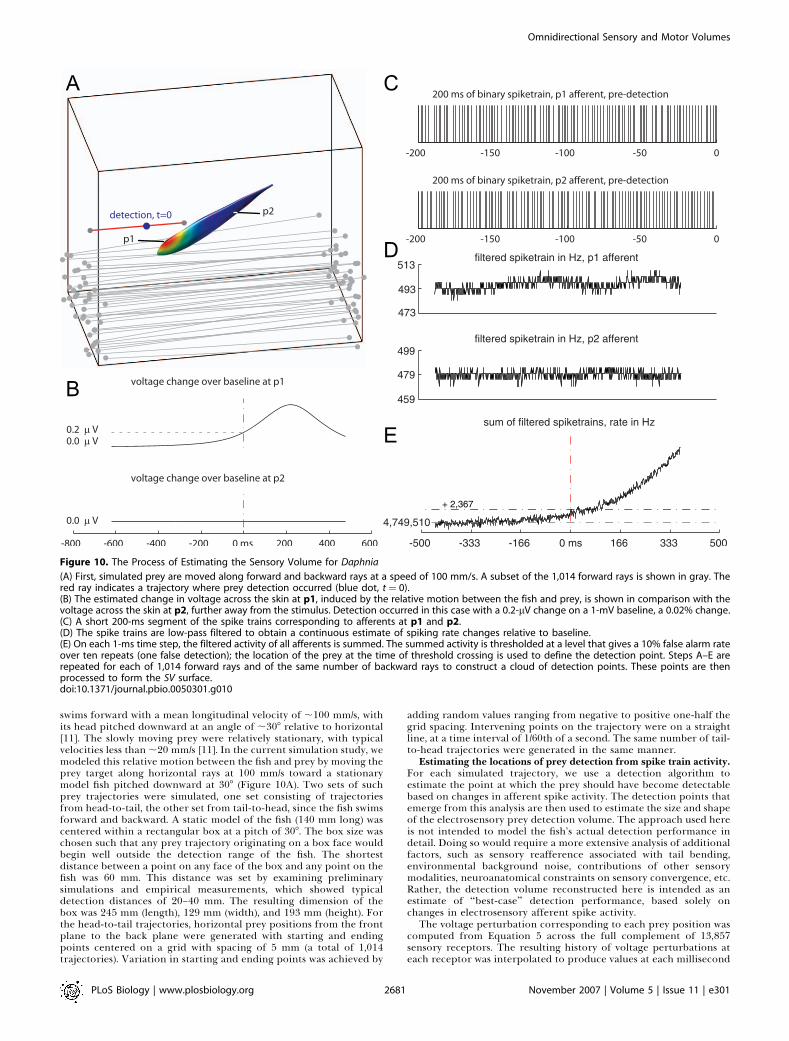
Figure 10. The Process of Estimating the Sensory Volume for Daphnia

(A) First, simulated prey are moved along forward and backward rays at a speed of 100 mm/s. A subset of the 1,014 forward rays is shown in gray. Thered ray indicates a trajectory where prey detection occurred (blue dot, t¼ 0).(B) The estimated change in voltage across the skin at p1, induced by the relative motion between the fish and prey, is shown in comparison with thevoltage across the skin at p2, further away from the stimulus. Detection occurred in this case with a 0.2-lV change on a 1-mV baseline, a 0.02% change.(C) A short 200-ms segment of the spike trains corresponding to afferents at p1 and p2.(D) The spike trains are low-pass filtered to obtain a continuous estimate of spiking rate changes relative to baseline.(E) On each 1-ms time step, the filtered activity of all afferents is summed. The summed activity is thresholded at a level that gives a 10% false alarm rateover ten repeats (one false detection); the location of the prey at the time of threshold crossing is used to define the detection point. Steps A–E arerepeated for each of 1,014 forward rays and of the same number of backward rays to construct a cloud of detection points. These points are thenprocessed to form the SV surface.doi:10.1371/journal.pbio.0050301.g010



and used as input for Equation 6. Because of the stochastic nature ofthe afferent model, ten spike trains were generated for each afferentvoltage history for each trial. Output spike trains for these synthetictrials were individually filtered using a boxcar filter with a windowsize s ¼ 200 ms, which in previous studies has corresponded to thebest weak signal detection capability [52]. At the end of eachmillisecond, we extract and sum the scalar activity level of each of the13,857 afferents. The motivation for this approach is that we assumethat any neural detection algorithm will require pooling ofinformation from multiple afferents; our goal here is not to specifyexactly how this pooling process takes place, but rather to evaluate abest-case scenario. Using the ‘‘no-stimulus’’ condition, a detectionthreshold was established at a level that yielded one false detectionper ten repeats. This detection strategy is a population-levelextension of the algorithm described by Goense and Ratnam [54]for detection of weak signals in an individual spike train with ISIcorrelations.

The prey detection distance was defined by the position of the preyat the time of threshold crossing for the ‘‘stimulus’’ condition. Foreach prey trajectory, the median and standard deviation of thedetection distances were computed over ten repeats. The number ofdetections over all trajectories formed a bimodal distribution, withone peak near one, corresponding to ‘‘false alarms’’ for trajectoriesoutside of the detection range, and a second peak near ten,corresponding to ‘‘true hits’’ for detections well within sensoryrange. There was a minimum in the bimodal distribution aroundseven, and we retained all trajectories with eight or more detections(out of ten) for further analysis. The mean and standard deviation ofthe detection distance for the resulting cloud of detection points wascomputed. To create the SV, this point cloud was triangulated into asmooth 3-D surface representation using a commercial softwarepackage (RapidForm, INUS Technology, Seoul, South Korea).

Measured prey encounter trajectories. The synthetic prey capturedistance results were validated by following the same methodologyoutlined above using measured prey encounter trajectories froman earlier study [11]. The earlier study found best detectionperformance for trials in low conductivity water most similar to thewater of the fish’s native habitat. Therefore, we examined only thissubset (35 lS/cm, N¼ 38). In our prior study, the measured detectionlocations were estimated by examining the first change in behaviornear to the prey [11] and therefore include sensorimotor delay time.Thus, to compare these to the computed neural detection points, weretrieved the distance between the prey and the fish at the detectiontime minus the sensorimotor delay time (115 ms [55]).

Motor volume (MV). The estimation of MV from motion capturedata does not assume the fish is stationary at the initial time step;rather,MV is estimated over all the initial velocities typical of our preycapture behavioral segments starting from just before detection tocapture, which includes forward as well as backward velocities, inaddition to heave (up in the body frame), and angular velocities suchas roll and pitch. It is defined in the coordinate frame at the fish’sinitial position (see Text S1 for details). We consider both theMVðV 90;� TÞ, where V 90 is the initial velocity in the coordinate framefixed to the fish’s initial position, for the entire body surface, MVbody,as well as the 3-D motor volume for the mouth alone, MVmouth.

The MV was computed from the 3-D fish surface trajectory dataobtained from 116 reconstructed prey-capture trials from an earlierstudy [11]. Because the motor volume for the mouth is a subset of thisspace, we will simply refer to the full volume as the MV, unless thedistinction between mouth and body volumes is relevant.MVðV 90;� TÞ was estimated from the trajectory data at fourteendifferent times T, ranging from 117 to 700 ms. For a given T, thenodes on the surface of the polygonal fish model at time tinitþT weretransformed back into the body-centered coordinate system of thefish at time tinit . This was repeated over all possible starting times tinitfor each trajectory (every 1/60th of a second up to the length of thetrial minus T), thus uniformly sampling all observed velocities. Theresult of this procedure was a dense point cloud, representing wherepoints on the fish’s surface can reach over time T. The points on thesurface of this cloud delineate an empirical estimation ofMVðV 90;� TÞ (Equation S1) in the absence of the equation ofmotion (Equation 1) and feasible control histories, as discussed in theIntroduction. The surface of the motor volume at each of the 14intervals was defined by binning of the point cloud around the fishinto voxels (5 3 5 3 5 mm), smoothing the data with a 3-D Gaussianconvolution kernel (standard deviation, 5 mm), and setting athreshold to include all voxels with point counts up to the 95thpercentile. Each resulting point cloud was triangulated to form closedpolyhedra for further analysis using commercial software (Rapid-Form, INUS Technology, Seoul, South Korea). The motor volume for

the mouth was constructed following the same procedure as for thebody, but using only a single node at the rostrum of the polygonalbody model. Because only a single node was used, the resulting pointcloud was less dense than the body point cloud. To accommodate thelower density, we maintained all voxels with point counts up to the90th percentile (rather than the 95th percentile used for the body)when constructing MVmouth.

The stopping volume was constructed similarly, but for compar-ison of the stopping volume to the SV, we restrict our selection oftrials to those of the same conductivity as used for estimating the SV,a total of 38 trials at 35 lS/cm. Unlike theMV,MVstop is not a functionof a fixed time T but rather depends on the set of initial velocities V 90from which we monitor movement until zero velocity is reached (seeText S1). Thus, we examine the volume swept by the body from thebehavioral reaction (detection) time minus the sensorimotor delaytime (115 ms, [55]) to the time at which the longitudinal velocity ofthe body is zero. We take the union of these 38 volumes to derive thestopping volume over all 35 lS/cm trials.

Computing environment. Computations were performed on a 54CPU (2 GHz G5, 1 GB RAM) cluster of Xserves (Apple Computer,Cupertino, California, USA) running OS X. An open-sourcedistributed computing engine (Grid Engine, Sun Microsystems, SantaClara, California, USA) was used to manage the computation acrossthe nodes. Simulation and analysis programs were written inMATLAB (The Mathworks, Nantick, Massachusetts, USA) andcompiled to portable executables for execution on the cluster.

Supporting Information

Interactive 3D visualizations of the sensory volume for prey (waterfleas, D. magna) (SV), time-limited motor volume (MV), and stoppingmotor volume (MVstop) for A. albifrons, the black ghost knifefish.These Virtual Reality Markup Language (VRML) models can beviewed using downloadable web browser plugins and external viewersavailable for many platforms.As of the date of publication, one of the following is recommended,in order of preference:Cortona VRML plugin (Windows and Mac OS X; available at: http://www.parallelgraphics.com/products/cortona).Octaga VRML player (Windows, Mac OS X. and Linux; available at:http://www.octaga.com/).Xj3D viewer (Windows, Mac OS X. and Linux; available at: http://www.web3d.org/x3d/xj3d/).

Figure S1. Interactive 3-D Version of Figure 3

Found at doi:10.1371/journal.pbio.0050301.sg001 (1.3 MB VRML).

Figure S2. Interactive 3-D Version of Figure 6A


Figure S3. Interactive 3-D Version of Figure 6B


Figure S4. Sensory Volume (Red) and Time-Limited Motor VolumeMVðV 90;� TÞ (Blue) at the Time of Maximal Overlap between SV andMV (t ¼ 432 ms)


Figure S5. Interactive 3-D Version of Figure 6C






Text S1. Technical Definition of Motor Volume and Stopping MotorVolume

Found at doi:10.1371/journal.pbio.0050301.sd001

Acknowledgments

We thank Kevin Lynch for generous assistance with the definition ofthe reachable set and motor volume.

Author contributions. MAM, JWB, and JBS conceived and designedthe experiments. JBS and MAM performed the experiments andanalyzed the data. MAM, MEN, and JBS wrote the paper.



Funding. This work was funded by the US National ScienceFoundation (NSF) grant IOB-0517683 (MAM), the Chicago Biomed-ical Consortium with support from The Searle Funds at The ChicagoCommunity Trust, NSF grant 0422073 (MEN), and the Engineering

Research Centers Program of the NSF under grant EEC-9402726(JWB).

Competing interests. The authors have declared that no competinginterests exist.

References1. Nelson ME, MacIver MA (2006) Sensory acquisition in active sensing

systems. J Comp Physiol A, Sensory, Neural, Behav Physiol 192: 573–586.2. Laughlin SB (2001) Energy as a constraint on the coding and processing of

sensory information. Curr Opin Neurobiol 11: 475–480.3. Dusenbery DB (1992) Sensory ecology: how organisms acquire and respond

to information. New York: W.H. Freeman. xx, 558 pp.4. Schnitzler H, Kalko EKV (2001) Echolocation by insect-eating bats.

BioScience 51: 557–569.5. Evans WE (1973) Echolocation by marine delphinids and one species of

fresh-water dolphin. J Acoust Soc Am 54: 191–199.6. Au WWL, Snyder KJ (1980) Long-range target detection in open waters by

an echolocating atlantic bottlenose dolphin (Tursiops truncatus). J AcoustSoc Am 68: 1077–1084.

7. Jones G (1999) Scaling of echolocation call parameters in bats. J Exp Biol202: 3359–3367.

8. Hartley DJ (1992) Stabilization of perceived echo amplitudes in echolocat-ing bats. I. Echo detection and automatic gain control in the big brown bat,Eptesicus fuscus, and the fishing bat, Noctilio leporinus. J Acoust Soc Am 91:1120–1132.

9. Tian B, Schnitzler H (1997) Echolocation signals of the Greater Horseshoebat (Rhinolophus ferrumequinum) in transfer flight and during landing. JAcoust Soc Am 101: 2347–2364.

10. Bastian J (1986) Electrolocation: behavior, anatomy, and physiology. In:Bullock TH, Heiligenberg W, editors. Electroreception. New York: Wiley.pp. 577–612.

11. MacIver MA, Sharabash NM, Nelson ME (2001) Prey-capture behavior ingymnotid electric fish: Motion analysis and effects of water conductivity. JExp Biol 204: 543–557.

12. Nelson ME, MacIver MA (1999) Prey capture in the weakly electric fishApteronotus albifrons: Sensory acquisition strategies and electrosensoryconsequences. J Exp Biol 202: 1195–1203.

13. Lannoo MJ, Lannoo SJ (1993) Why do electric fishes swim backwards? Anhypothesis based on Gymnotiform foraging behavior interpreted throughsensory constraints. Environ Biol Fishes 36: 157–165.

14. Choset HM, Lynch KM, Hutchinson S, Kantor G, Burgard W, et al. (2005)Nonholonomic and underactuated systems. In: Principles of robot motion:theory, algorithms, and implementation. Cambridge (Massachusetts): MITPress. pp. 401–472.

15. Sastry SS (1999) Geometric nonlinear control. In: Nonlinear systems:analysis, stability, and control. New York: Springer. pp. 510–573.

16. LaValle SM (2006) Sampling-based planning under differential constraints.In: Planning algorithms. New York: Cambridge University Press. pp. 787–860.

17. Reeds JA, Shepp LA (1990) Optimal paths for a car that goes both forwardsand backwards. Pacific J Math 145: 367–393.

18. Vendittelli M, Laumond JP, Nissoux C (1999) Obstacle distance for car-likerobots. IEEE Trans Robotics Automation 15: 678–691.

19. MacIver MA (2001) The computational neuroethology of weakly electricfish: Body modeling, motion analysis, and sensory signal estimation. [PhDdissertation] Urbana (Illinois): Program in Neuroscience, University ofIllinois. 187 p.

20. Rasnow B, Bower JM (1996) The electric organ discharges of thegymnotiform fishes: I. Apteronotus leptorhynchus. J Comp Physiol A, Sensory,Neural, Behav Physiol 178: 383–396.

21. Nelson ME, Xu Z, Payne J (1997) Characterization and modeling of P-typeelectrosensory afferent response dynamics in the weakly electric fishAperonotus leptorhynchus. J Comp Physiol A, Sensory, Neural, Behav Physiol181: 532–544.

22. Julian D, Crampton WGR, Wohlgemuth SE, Albert JS (2003) Oxygenconsumption in weakly electric Neotropical fishes. Oecologia 137: 502–511.

23. Bell CC, Bradbury J, Russell CJ (1976) The electric organ of a mormyrid as acurrent and voltage source. J Comp Physiol 110: 65–88.

24. Nelson ME, MacIver MA, Coombs S (2002) Modeling electrosensory andmechanosensory images during the predatory behavior of weakly electricfish. Brain Behav Evol 59: 199–210.

25. Kalko EK (1995) Insect pursuit, prey capture and echolocation in pipistrellebats (Microchiroptera). Anim Behav 50: 861–880.

26. Wotton JM, Jenison RL, Hartley DJ (1997) The combination of echolocationemission and ear reception enhances directional spectral cues of the bigbrown bat, Eptesicus fuscus. J Acoust Soc Am 101: 1723–1733.

27. Henze D, O’Neill WE (1991) The emission pattern of vocalizations anddirectionality of the sonar system in the echolocating bat, Pteronotus parnelli.J Acoust Soc Am 89: 2430–2434.

28. Ghose K, Moss CF (2003) The sonar beam pattern of a flying bat as it trackstethered insects. J Acoust Soc of Am 114: 1120–1131.

29. Holderied MW, von Helversen O (2003) Echolocation range and wingbeatperiod match in aerial-hawking bats. Proc R Soc Lond Series B: Biol Sci270: 2293–2299.

30. Erwin HR, Wilson WW, Moss CF (2001) A computational sensorimotormodel of bat echolocation. J Acoust Soc Am 110: 1176–1187.

31. Madsen PT, Kerr I, Payne R (2004) Echolocation clicks of two free-ranging,oceanic delphinids with different food preferences: false killer whalesPseudorca crassidens and Risso’s dolphins Grampus griseus. J Exp Biol 207:1811–1823.

32. Dunbrack RL, Dill LM (1984) 3-Dimensional Prey Reaction Field of theJuvenile Coho Salmon (Oncorhynchus-Kisutch). Can J Fish Aquatic Sci 41:1176–1182.

33. Luecke C, Obrien WJ (1981) Prey location volume of a planktivorous fish - anew measure of prey vulnerability. Can J Fish Aquatic Sci 38: 1264–1270.

34. Wanzenbock J, Scheimer F (1989) Prey detection in cyprinids during earlydevelopment. Can J Fish Aquatic Sci 46: 995–1001.

35. Link J (1998) Dynamics of lake herring (Coregonus artedi) reactive volume fordifferent crustacean zooplankton. Hydrobiologia 368: 101–110.

36. Asaeda T, Park BK, Manatunge J (2002) Characteristics of reaction field andthe reactive distance of a planktivore, Pseudorasbora parva (Cyprinidae), invarious environmental conditions. Hydrobiologia 489: 29–43.

37. Flore L, Reckendorfer W, Keckeis H (2000) Reaction field, capture field,and search volume of 0þ nase (Chondrostoma nasus): effects of body size andwater velocity. Can J Fish Aquatic Sci 57: 342–350.

38. Shkel AM, Lumelsky VJ (1997) Incorporating body dynamics into sensor-based motion planning: The maximum turn. IEEE Trans RoboticsAutomation 13: 873–880.

39. MacIver MA (2008) Neuroethology: from morphological computation toplanning. In: Robbins P, Aydede M, editors. Cambridge Handbook ofSituated Cognition. Cambridge (United Kingdom: Cambridge UniversityPress (In press).

40. MacIver MA, Nelson ME (2000) Body modeling and model-based trackingfor neuroethology. J Neurosci Method 95: 133–143.

41. Chen L, House JL, Krahe R, Nelson ME (2005) Modeling signal andbackground components of electrosensory scenes. J Comp Physiol A,Sensory, Neural, Behav Physiol 191: 331–345.

42. Assad C, Rasnow B, Stoddard PK (1999) Electric organ discharges andelectric images during electrolocation. J Exp Biol 202: 1185–1193.

43. Knudsen EI (1975) Spatial aspects of the electric fields generated by weaklyelectric fish. J Comp Physiol A, Sensory, Neural, Behav Physiol 99: 103–118.

44. Carr CE, Maler L, Sas E (1982) Peripheral organization and centralprojections of the electrosensory nerves in Gymnotiform fish. J CompNeurol 211: 139–153.

45. Hagiwara S, Szabo T, Enger PS (1965) Electroreceptor mechanisms in ahigh-frequency weakly electric fish, Sternarchus albifrons. J Neurophysiol 28:784–799.

46. Szabo T (1974) Anatomy of the specialized lateral line organs of electro-reception. In: Fessard A, editor. Electroreceptors and other specializedreceptors in lower vertebrates (Handbook of sensory physiology, vol III).New York: Springer. pp. 13–58.

47. Rasnow B (1996) The effects of simple objects on the electric field ofApteronotus. J Comp Physiol A, Sensory, Neural, Behav Physiol 178: 397–411.

48. Brandman R, Nelson ME (2002) A simple model of long-term spike trainregularization. Neural Comput 14: 1575–1597.

49. Chacron MJ, Longtin A, Maler M (2001) Negative interspike intervalcorrelations increase the neuronal capacity for encoding time-dependentstimuli. J Neurosci 21: 5328–5343.

50. Chacron MJ, Lindner B, Longtin A (2004) Noise shaping by intervalcorrelations increases information transfer. Phys Rev Lett 92. doi:10.1103/PhysRevLett.92.080601.

51. Knudsen EI (1974) Behavioral thresholds to electric signals in highfrequency electric fish. J Comp Physiol 91: 333–353.

52. Ratnam R, Nelson ME (2000) Non-renewal statistics of electrosensoryafferent spike trains: implications for the detection of weak sensory signals.J Neurosci 20: 6672–6683.

53. Xu Z, Payne JR, Nelson ME (1996) Logarithmic time course of sensoryadaptation in electrosensory afferent nerve fibers in a weakly electric fish. JNeurophysiol 76: 2020–2032.

54. Goense JBM, Ratnam R (2003) Continuous detection of weak sensorysignals in afferent spike trains: the role of anti-correlated interspikeintervals in detection performance. J Comp Physiol A, Sensory, Neural,Behav Physiol 189: 741–759.

55. Bastian J (1987) Electrolocation in the presence of jamming signals:behavior. J Comp Physiol A, Sensory, Neural, Behav Physiol 161: 811–824.



Documents

PLoS BIOLOGY Omnidirectional Sensory and Motor Volumes in