Embed Size (px)
Citation preview
plink: An R Package for Linking Mixed-Format
Tests Using IRT-Based Methods
Jonathan P. WeeksUniversity of Colorado at Boulder
Abstract
This introduction to the R package plink is a (slightly) modified version of Weeks(2010), published in the Journal of Statistical Software.
The R package plink has been developed to facilitate the linking of mixed-format testsfor multiple groups under a common item design using unidimensional and multidimen-sional IRT-based methods. This paper presents the capabilities of the package in thecontext of the unidimensional methods. The package supports nine unidimensional itemresponse models (the Rasch model, 1PL, 2PL, 3PL, graded response model, partial creditand generalized partial credit model, nominal response model, and multiple-choice model)and four separate calibration linking methods (mean/sigma, mean/mean, Haebara, andStocking-Lord). It also includes functions for importing item and/or ability parametersfrom common IRT software, conducting IRT true-score and observed-score equating, andplotting item response curves and parameter comparison plots.
Keywords: item response theory, separate calibration, chain linking, mixed-format tests, R.
1. Introduction
In many measurement scenarios there is a need to compare results from multiple tests, butdepending on the statistical properties of these measures and/or the sample of examinees,scores across tests may not be directly comparable; in most instances they are not. Tocreate a common scale, scores from all tests of interest must be transformed to the metricof a reference test. This process is known generally as linking, although other terms likeequating and vertical scaling are often used to refer to specific instantiations (see Linn 1993,for information on the associated terminology). Linking methods were originally developed toequate observed scores for parallel test forms (Hull 1922; Kelley 1923; Gulliksen 1950; Levine1955). These approaches work well when the forms are similar in terms of difficulty andreliability, but as the statistical specifications of the tests diverge, the comparability of scoresacross tests becomes increasingly unstable (Petersen, Cook, and Stocking 1983; Yen 1986).
Thurstone (1925, 1938) developed observed score methods for creating vertical scales when thedifficulties of the linked tests differ substantively. These methods depend on item p-values orempirical score distributions which are themselves dependent on the sample of examinees andthe particular items included on the tests. As such, these approaches can be unreliable. Lordand Novick (1968) argued that in order to maintain a consistent scale, the linking approachmust be based on a stable scaling model (i.e., a model with invariant item parameters). Withthe advent of item response theory (IRT; Lord 1952; Lord and Novick 1968; Lord 1980)

2 plink: Linking Mixed-Format Tests Using IRT-Based Methods in R
this became possible. Today, IRT-based linking is the most commonly used approach fordeveloping vertical scales, and it is being used increasingly for equating (particularly in thedevelopment of calibrated item banks).
The R (R Development Core Team 2010) package plink, available from the ComprehensiveR Archive Network at http://CRAN.R-project.org/package=plink, was developed to fa-cilitate the linking of mixed-format tests for multiple groups under a common item design(Kolen and Brennan 2004) using unidimensional and multidimensional IRT-based methods.The aim of this paper is to present the package with a specific focus on the unidimensionalmethods. An explication of the multidimensional methods will be described in a future arti-cle. This paper is divided into three main sections and two appendices. Section 2 providesan overview of the item response models and linking methods supported by plink. Section 3describes how to format the various objects needed to run the linking function, and Section4 illustrates how to link a set of tests using the plink function. Appendix A provides a briefdescription of additional features, and Appendix B.1 presents a comparison and critique ofavailable linking software.
2. Models and methods
plink supports nine1 unidimensional item response models (the Rasch model, 1PL, 2PL,3PL, graded response model, partial credit and generalized partial credit model, nominalresponse model, and multiple-choice model) and four separate calibration linking methods(mean/sigma, mean/mean, Haebara, and Stocking-Lord). All of these models and methodsare well documented in the literature, although the parameterizations can vary. The followingtwo sub-sections are included to acquaint the reader with the specific parameterizations usedin the package.
2.1. Item response models
Let the variable Xij represent the response of examinee i to item j. Given a test consisting ofdichotomously scored items, Xij = 1 for a correct item response, and Xij = 0 for an incorrectresponse. The response probabilities for the three-parameter logistic model (3PL; Birnbaum1968) take the following form
Pij = P (Xij = 1|θi, aj , bj , cj) = cj + (1− cj)exp [Daj (θi − bj)]
1 + exp [Daj (θi − bj)](1)
where θi is an examinee’s ability on a single construct, aj is the item discrimination, bj is theitem difficulty, cj is the lower asymptote (guessing parameter), and D is a scaling constant.
If the guessing parameter is constrained to be zero, Equation 1 becomes the two-parameterlogistic model (2PL; Birnbaum 1968), and if it is further constrained so that the discriminationparameters for all items are equal, it becomes the one-parameter logistic model (1PL). TheRasch model (Rasch 1960) is a special case of the 1PL where all of the item discriminationsare constrained to equal one.
When items are polytomously scored (i.e., items with three or more score categories), theresponse Xij is coded using a set of values k = {1, ...,Kj} where Kj is the total number of
1By constraining the parameters in these models, other models like Andrich’s (1978) rating scale model orSamejima’s (1979) extension of the nominal response model can be specified.
Jonathan P. Weeks 3
categories for item j. When the values of k correspond to successively ordered categories,the response probabilities can be modeled using either the graded response model (GRM;Samejima 1969) or the generalized partial credit model (GPCM; Muraki 1992). The gradedresponse model takes the following form
P̃ijk = P̃ (Xij = k|θi, aj , bjk) =
1 k = 1
exp [Daj (θi − bjk)]1 + exp [Daj (θi − bjk)]
2 ≤ k ≤ Kj
0 k > Kj
(2)
where aj is the item slope and bjk is a threshold parameter. The threshold parameters can bealternately formatted as deviations from an item-specific difficulty commonly referred to as alocation parameter. That is, bjk can be respecified as bj + gjk where the location parameterbj is equal to the mean of the bjk and the gjk are deviations from this mean.
In Equation 2, the P̃ijk correspond to cumulative probabilities, yet the equation can be refor-mulated to identify the probability of responding in a given category. This is accomplished bytaking the difference between the P̃ijk for adjacent categories. These category probabilitiesare formulated as
Pijk = P̃ijk − P̃ij(k+1). (3)
The generalized partial credit model takes the following form
Pijk = P (Xij = v|θi, aj , bjk) =
exp
[k∑
v=1
Daj (θi − bjv)
]Kj∑h=1
exp
[h∑
v=1
Daj (θi − bjv)
] (4)
where bjk is an intersection or step parameter. As with the graded response model, the bjk foreach item can be reformulated to include a location parameter and step-deviation parameters(e.g., bj + gjk). Further, the slope parameters for the GPCM can be constrained to be equalacross all items. When they equal one, this is known as the partial credit model (PCM;Masters 1982). For both the PCM and the GPCM, the parameter bj1 can be arbitrarily setto any value because it is cancelled from the numerator and denominator (see Muraki 1992for more information). For all of the functions in plink that use either of these models, bj1 isexcluded, meaning only Kj − 1 step parameters should be specified.
The GRM, PCM, and GPCM assume that the values for k correspond to successively orderedcategories, but if the responses are not assumed to be ordered, they can be modeled usingthe nominal response model (NRM; Bock 1972) or the multiple-choice model (MCM; Thissenand Steinberg 1984). The nominal response model takes the following form
Pijk = P (Xij = k|θi, ajk, bjk) =exp (ajkθi + bjk)
Kj∑h=1
exp (ajhθi + bjh)
(5)
where ajk is a category slope and bjk is a category “difficulty” parameter. For the purpose ofidentification, the model is typically specified under the constraint that
4 plink: Linking Mixed-Format Tests Using IRT-Based Methods in R
Kj∑k=1
ajk = 0 and
Kj∑k=1
bjk = 0.
The final model supported by plink is the multiple-choice model. It is an extension of the NRMthat includes lower asymptotes on each of the response categories and additional parametersfor a “do not know” category. The model is specified as
Pijk = P (Xij = k|θi, ajk, bjk, cjk) =exp (ajkθi + bjk) + cjk exp (aj0θi + bj0)
Kj∑h=0
exp (ajhθi + bjh)
(6)
where Kj is equal to the number of actual response categories plus one, aj0 and bj0 are theslope and category parameters respectively for the “do not know” category, and ajk and bjkhave the same interpretation as the parameters in Equation 5. This model is typically identi-fied using the same constraints on ajk and bjk as the NRM, and given that cjk represents theproportion of individuals who “guessed” a specific distractor, the MCM imposes an additionalconstraint, where
Kj∑k=1
cjk = 1.
2.2. Calibration methods
The ultimate goal of test linking is to place item parameters and/or ability estimates fromtwo or more tests onto a common scale. When there are only two tests, this involves findinga set of linking constants to transform the parameters from one test (the from scale) to thescale of the other (the to scale). The parameters associated with these tests are subscriptedby an F and T respectively. When there are more than two tests, linking constants are firstestimated for each pair of “adjacent” tests (see Section 3.4) and then chain-linked together toplace the parameters for all tests onto a base scale. For a given pair of tests, the equation totransform θF to the θT scale is
θT = AθF +B = θ∗F (7)
where the linking constants A and B are used to adjust the standard deviation and meanrespectively, and the ∗ denotes a transformed value on the to scale. See Kim and Lee (2006) foran explanation of the properties and assumptions of IRT that form the basis for this equation,the following transformations, and a more detailed explanation of the linking methods.
Since the item parameters are inextricably tied to the θ scale, any linear transformation ofthe scale will necessarily change the item parameters such that the expected probabilities willremain unchanged. As such, it can be readily shown that aj and bjk for the GRM, GPCM,and dichotomous models on the from scale can be transformed to the to scale by
a∗jF = ajF /A (8a)
b∗jkF = AbjkF +B (8b)
where the constants A and B are the same as those used to transform θF (Lord and Novick1968; Baker 1992). Since the NRM and MCM are parameterized using a slope/intercept
Jonathan P. Weeks 5
formulation (i.e., ajkθi + bjk) rather than a slope/difficulty formulation (i.e., aj [θi− bjk]), theslopes and category parameters are transformed using (Baker 1993a; Kim and Hanson 2002)
a∗jkF = ajkF /A (9a)
b∗jkF = bjkF − (B/A) ajkF . (9b)
When lower asymptote parameters are included in the model, as with the 3PL and MCM,they are unaffected by the transformation; hence, c∗jF = cjF .
Equations 7 to 9b illustrate the transformation of item and ability parameters from the fromscale to the to scale; however, a reformulation of these equations can be used to transformthe parameters on the to scale to the from scale. These transformations are important whenconsidering symmetric linking (discussed later). The item parameters for the GRM, GPCMand dichotomous models are transformed by
a#jT = AajT (10a)
b#jkT = (bjkT −B) /A (10b)
and the item parameters for the NRM and MCM are transformed by
a#jkT = AajkT (11a)
b#jkT = bjkT +BajkT (11b)
where the # denotes a transformed value on the From scale. Again, the lower asymptoteparameters remain unaffected, so c#jT = cjT .
This package supports four of the most commonly used methods for estimating linking con-stants under an equivalent or non-equivalent groups common item design (Kolen and Brennan2004). Within this framework, a subset of S ≤ J common items between the to and fromtests are used to estimate the constants. The mean/sigma (Marco 1977) and mean/mean(Loyd and Hoover 1980) methods, known as moment methods, are the simplest approachesto estimating A and B because they only require the computation of means and standarddeviations for various item parameters. For the mean/sigma, only the bsk are used. That is,
A =σ(bT )
σ(bF )(12a)
B = µ(bT )−Aµ(bF ) (12b)
where the means and standard deviations are taken over all S common items and Ks responsecategories. One potential limitation of this approach, however, is that it does not consider theslope parameters. The mean/mean, on the other hand, uses both the ask and bsk to estimatethe linking constants where
A =µ(aF )
µ(aT )(13a)
B = µ(bT )−Aµ(bF ). (13b)
Both of these approaches assume that the items are parameterized using a slope/difficultyformulation, but because NRM and MCM items use a slope/intercept parameterization, the
6 plink: Linking Mixed-Format Tests Using IRT-Based Methods in R
bsk must be reformulated as b̃sk = −bsk/ask before computing the means and standard devi-ations. Given this reparameterization, there are several issues related to the use of NRM andMCM items with the moment methods (see Kim and Lee 2006, for more information).
As an alternative to the moment methods, Haebara (1980) and Stocking and Lord (1983)developed characteristic curve methods that use an iterative approach to estimate the linkingconstants by minimizing the sum of squared differences between item characteristic curvesand test characteristic curves for the common items for the two methods respectively. Thesemethods are typically implemented by finding the constants that best characterize the fromscale parameters on the to scale; however, this assumes that the parameters on the to scalewere estimated without error. For this reason, Haebara (1980) proposed a criterion thatsimultaneously considers the transformation of parameters from the from scale to the toscale and vice-versa. The former case—the typical implementation—is referred to as a non-symmetric approach and the later is referred to as a symmetric approach.
The Haebara method minimizes the following criterion
Q = Q1 +Q2 (14a)
where
Q1 =1
L1
M∑m=1
S∑s=1
Ks∑k=1
[Psk (θmT )− P ∗sk (θmT )]2W1 (θmT ) (14b)
and
Q2 =1
L2
M∑m=1
S∑s=1
Ks∑k=1
[Psk (θmF )− P#
sk (θmF )]2W2 (θmF ) (14c)
where
L1 =
M∑m=1
W1 (θmT )
S∑s=1
Ks and L2 =
M∑m=1
W2 (θmF )
S∑s=1
Ks.
The θmT are a set of M points on the to scale where differences in expected probabilities areevaluated, Psk (θmT ) are expected probabilities based on the untransformed to scale commonitem parameters, P ∗
sk (θmT ) are expected probabilities based on the transformed from scalecommon item parameters, and the W1 (θmT ) are a set of quadrature weights corresponding toθmT . The θmF are a set of points on the from scale where differences in expected probabilitiesare evaluated, Psk (θmF ) are expected probabilities based on the untransformed from scale
common item parameters, P#sk (θmF ) are expected probabilities based on the transformed to
scale common item parameters, and the W2 (θmF ) are a set of quadrature weights correspond-ing to θmF . L1 and L2 are constants used to standardize the criterion function to prevent thevalue from exceeding upper or lower bounds in the optimization. The inclusion of L1 and L2
does not affect the estimated linking constants (Kim and Lee 2006). Q is minimized in thesymmetric approach, but only Q1 is minimized in the non-symmetric approach.
The Stocking-Lord method minimizes the following criterion
F = F1 + F2 (15a)
where
F1 =1
L∗1
M∑m=1
[S∑
s=1
Ks∑k=1
UskPsk (θmT )−S∑
s=1
Ks∑k=1
UskP∗sk (θmT )
]2
W1 (θmT ) (15b)

Jonathan P. Weeks 7
and
F2 =1
L∗2
M∑m=1
[S∑
s=1
Ks∑k=1
UskPsk (θmF )−S∑
s=1
Ks∑k=1
UskP#sk (θmF )
]2
W2 (θmF ) (15c)
where
L∗1 =
M∑m=1
W1 (θmT ) and L∗2 =
M∑m=1
W2 (θmF ).
To create the test characteristic curves, the scoring function Usk must be included to weighteach response category. These values are typically specified as Usk = {0, ...,Ks − 1}, whichassumes that the categories are ordered. F is minimized in the symmetric approach, but onlyF1 is minimized in the non-symmetric approach.
3. Preparing the data
There are four necessary elements that must be created to prepare the data prior to linkinga set of tests using the function plink:
1. an object containing the item parameters,
2. an object specifying the number of response categories for each item,
3. an object identifying the item response models associated with each item,
4. an object identifying the common items between groups.
In short, these elements create a blueprint of the unique and common items across two ormore tests. The following section describes how to specify the first three elements for asingle set of item parameters then shows how the elements for two or more groups can becombined—incorporating the common item object—for use in plink. The section concludeswith a discussion of methods for importing data from commonly used IRT estimation software.If the parameters are imported from one of the software packages identified in Section 3.5, noadditional formatting is required (i.e., Sections 3.1, 3.2, and 3.3 can be skipped).
3.1. Formatting the item parameters
The key elements of any IRT-based linking method—using a common item design—are theitem parameters, but depending on the program used to estimate them, they may comein a variety of formats. plink is designed to allow a fair amount of flexibility in how theparameters are specified to minimize the need for reformatting. This object, named x in allrelated functions, can be specified for single-format or mixed-format items as a vector, matrix,or list.
Vector formulation
When the Rasch model is used, x can be formatted as a vector of item difficulties, but for allother models a matrix or list specification must be used (the Rasch model can be specifiedusing these formulations as well).
8 plink: Linking Mixed-Format Tests Using IRT-Based Methods in R
Matrix formulation
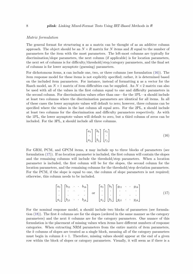
The general format for structuring x as a matrix can be thought of as an additive columnapproach. The object should be an N ×R matrix for N items and R equal to the number ofparameters for the item with the most parameters. The left-most columns are typically fordiscrimination/slope parameters, the next column (if applicable) is for location parameters,the next set of columns is for difficulty/threshold/step/category parameters, and the final setof columns is for lower asymptote (guessing) parameters.
For dichotomous items, x can include one, two, or three columns (see formulation (16)). Theitem response model for these items is not explicitly specified; rather, it is determined basedon the included item parameters. For instance, instead of formatting x as a vector for theRasch model, an N × 1 matrix of item difficulties can be supplied. An N × 2 matrix can alsobe used with all of the values in the first column equal to one and difficulty parameters inthe second column. For discrimination values other than one—for the 1PL—x should includeat least two columns where the discrimination parameters are identical for all items. In allof these cases the lower asymptote values will default to zero; however, three columns can bespecified where the values in the last column all equal zero. For the 2PL, x should includeat least two columns for the discrimination and difficulty parameters respectively. As withthe 1PL, the lower asymptote values will default to zero, but a third column of zeros can beincluded. For the 3PL, x should include all three columns.
a1·aj
b1·bj
c1·cj
(16)
For GRM, PCM, and GPCM items, x may include up to three blocks of parameters (seeformulation (17)). If no location parameter is included, the first column will contain the slopesand the remaining columns will include the threshold/step parameters. When a locationparameter is included, the first column will be for the slopes, the second column for thelocation parameters, and the remaining columns for the threshold/step deviation parameters.For the PCM, if the slope is equal to one, the column of slope parameters is not required;otherwise, this column needs to be included.
a1··aj
b11 · · b1k· · ·· · ·bj1 · · bjk
or
a1··aj
b1··bj
g11 · · g1k· · ·· · ·gj1 · · gjk
(17)
For the nominal response model, x should include two blocks of parameters (see formula-tion (18)). The first k columns are for the slopes (ordered in the same manner as the categoryparameters) and the next k columns are for the category parameters. One nuance of thisformulation is the placement of missing values when items have different numbers of responsecategories. When extracting NRM parameters from the entire matrix of item parameters,the k columns of slopes are treated as a single block, meaning all of the category parametersmust begin in column k + 1. Therefore, missing values should appear at the end of a givenrow within the block of slopes or category parameters. Visually, it will seem as if there is a
Jonathan P. Weeks 9
gap in the middle of the row (see formulation (20)).
a11 · · a1k· · ·· · ·aj1 · · ajk
b11 · · b1k· · ·· · ·bj1 · · bjk
(18)
The specification of item parameters for the multiple-choice model is very similar to thespecification for NRM items with the only difference being the addition of a block of lowerasymptote parameters (see formulation (19)). The same placement of missing values applieshere as well.
a11 · · a1k· · ·· · ·aj1 · · ajk
b11 · · b1k· · ·· · ·bj1 · · bjk
c11 · c1k−1
· · ·· · ·cj1 · cjk−1
(19)
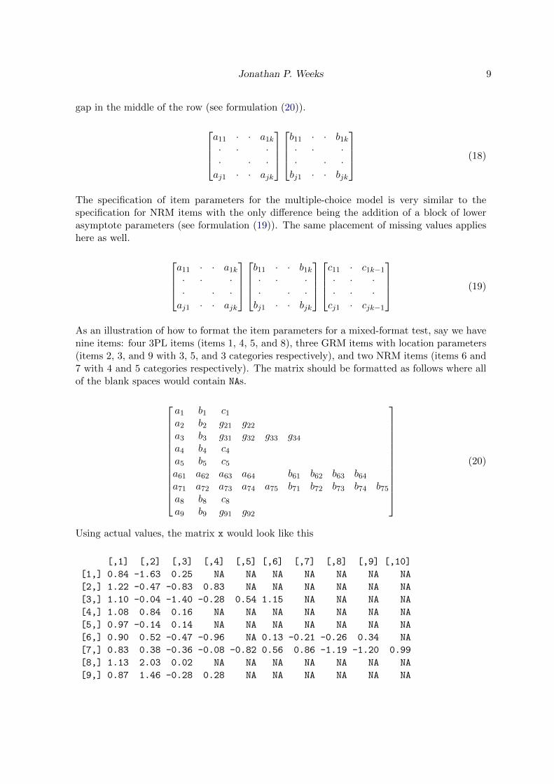
As an illustration of how to format the item parameters for a mixed-format test, say we havenine items: four 3PL items (items 1, 4, 5, and 8), three GRM items with location parameters(items 2, 3, and 9 with 3, 5, and 3 categories respectively), and two NRM items (items 6 and7 with 4 and 5 categories respectively). The matrix should be formatted as follows where allof the blank spaces would contain NAs.
a1 b1 c1a2 b2 g21 g22a3 b3 g31 g32 g33 g34a4 b4 c4a5 b5 c5a61 a62 a63 a64 b61 b62 b63 b64a71 a72 a73 a74 a75 b71 b72 b73 b74 b75a8 b8 c8a9 b9 g91 g92
(20)
Using actual values, the matrix x would look like this
[,1] [,2] [,3] [,4] [,5] [,6] [,7] [,8] [,9] [,10]
[1,] 0.84 -1.63 0.25 NA NA NA NA NA NA NA
[2,] 1.22 -0.47 -0.83 0.83 NA NA NA NA NA NA
[3,] 1.10 -0.04 -1.40 -0.28 0.54 1.15 NA NA NA NA
[4,] 1.08 0.84 0.16 NA NA NA NA NA NA NA
[5,] 0.97 -0.14 0.14 NA NA NA NA NA NA NA
[6,] 0.90 0.52 -0.47 -0.96 NA 0.13 -0.21 -0.26 0.34 NA
[7,] 0.83 0.38 -0.36 -0.08 -0.82 0.56 0.86 -1.19 -1.20 0.99
[8,] 1.13 2.03 0.02 NA NA NA NA NA NA NA
[9,] 0.87 1.46 -0.28 0.28 NA NA NA NA NA NA
10 plink: Linking Mixed-Format Tests Using IRT-Based Methods in R
List formulation
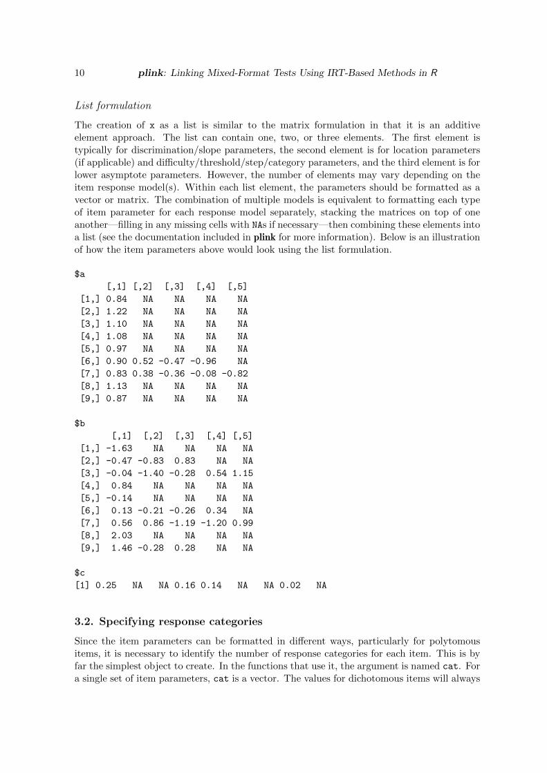
The creation of x as a list is similar to the matrix formulation in that it is an additiveelement approach. The list can contain one, two, or three elements. The first element istypically for discrimination/slope parameters, the second element is for location parameters(if applicable) and difficulty/threshold/step/category parameters, and the third element is forlower asymptote parameters. However, the number of elements may vary depending on theitem response model(s). Within each list element, the parameters should be formatted as avector or matrix. The combination of multiple models is equivalent to formatting each typeof item parameter for each response model separately, stacking the matrices on top of oneanother—filling in any missing cells with NAs if necessary—then combining these elements intoa list (see the documentation included in plink for more information). Below is an illustrationof how the item parameters above would look using the list formulation.
$a
[,1] [,2] [,3] [,4] [,5]
[1,] 0.84 NA NA NA NA
[2,] 1.22 NA NA NA NA
[3,] 1.10 NA NA NA NA
[4,] 1.08 NA NA NA NA
[5,] 0.97 NA NA NA NA
[6,] 0.90 0.52 -0.47 -0.96 NA
[7,] 0.83 0.38 -0.36 -0.08 -0.82
[8,] 1.13 NA NA NA NA
[9,] 0.87 NA NA NA NA
$b
[,1] [,2] [,3] [,4] [,5]
[1,] -1.63 NA NA NA NA
[2,] -0.47 -0.83 0.83 NA NA
[3,] -0.04 -1.40 -0.28 0.54 1.15
[4,] 0.84 NA NA NA NA
[5,] -0.14 NA NA NA NA
[6,] 0.13 -0.21 -0.26 0.34 NA
[7,] 0.56 0.86 -1.19 -1.20 0.99
[8,] 2.03 NA NA NA NA
[9,] 1.46 -0.28 0.28 NA NA
$c
[1] 0.25 NA NA 0.16 0.14 NA NA 0.02 NA
3.2. Specifying response categories
Since the item parameters can be formatted in different ways, particularly for polytomousitems, it is necessary to identify the number of response categories for each item. This is byfar the simplest object to create. In the functions that use it, the argument is named cat. Fora single set of item parameters, cat is a vector. The values for dichotomous items will always
Jonathan P. Weeks 11
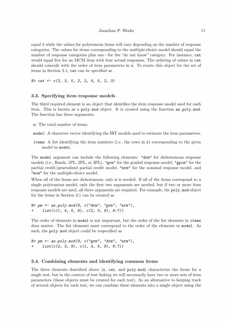
equal 2 while the values for polytomous items will vary depending on the number of responsecategories. The values for items corresponding to the multiple-choice model should equal thenumber of response categories plus one—for the “do not know” category. For instance, catwould equal five for an MCM item with four actual responses. The ordering of values in cat
should coincide with the order of item parameters in x. To create this object for the set ofitems in Section 3.1, cat can be specified as
R> cat <- c(2, 3, 5, 2, 2, 4, 5, 2, 3)
3.3. Specifying item response models
The third required element is an object that identifies the item response model used for eachitem. This is known as a poly.mod object. It is created using the function as.poly.mod.The function has three arguments:
n: The total number of items.
model: A character vector identifying the IRT models used to estimate the item parameters.
items: A list identifying the item numbers (i.e., the rows in x) corresponding to the givenmodel in model.
The model argument can include the following elements: "drm" for dichotomous responsemodels (i.e., Rasch, 1PL, 2PL, or 3PL), "grm" for the graded response model, "gpcm" for thepartial credit/generalized partial credit model, "nrm" for the nominal response model, and"mcm" for the multiple-choice model.
When all of the items are dichotomous, only n is needed. If all of the items correspond to asingle polytomous model, only the first two arguments are needed, but if two or more itemresponse models are used, all three arguments are required. For example, the poly.mod objectfor the items in Section 3.1 can be created as
R> pm <- as.poly.mod(9, c("drm", "grm", "nrm"),
+ list(c(1, 4, 5, 8), c(2, 3, 9), 6:7))
The order of elements in model is not important, but the order of the list elements in items
does matter. The list elements must correspond to the order of the elements in model. Assuch, the poly.mod object could be respecified as
R> pm <- as.poly.mod(9, c("grm", "drm", "nrm"),
+ list(c(2, 3, 9), c(1, 4, 5, 8), 6:7))
3.4. Combining elements and identifying common items
The three elements described above (x, cat, and poly.mod) characterize the items for asingle test, but in the context of test linking we will necessarily have two or more sets of itemparameters (these objects must be created for each test). As an alternative to keeping trackof several objects for each test, we can combine these elements into a single object using the
12 plink: Linking Mixed-Format Tests Using IRT-Based Methods in R
as.irt.pars function (this type of object is also required for plink). This function createsan irt.pars object that characterizes the items for one or more tests and includes built-invalidation checks to ensure that there are no obvious incongruences between the parameters,response categories, and item response models. The as.irt.pars function has the followingarguments:
x: An object containing item parameters. When multiple groups are present, x should be alist of parameter objects (a combination of objects using the vector, matrix, and/or listformulation).
common: An S× 2 matrix or list of matrices identifying the common items between adjacentgroups in x. This argument is only applicable when x includes two or more groups.
cat: A vector or list of vectors (for two or more groups) identifying the number of responsecategories.
poly.mod: A poly.mod object or list of poly.mod objects (for two or more groups).
dimensions: A numeric vector identifying the number of modeled dimensions in each group.The default is 1.
location: A logical vector indicating whether the parameters for each group in x include alocation parameter. The default is FALSE.
grp.names: A character vector of group names.
To create an irt.pars object for the single set of parameters specified in Section 3.1 we woulduse
R> pars <- as.irt.pars(x, cat = cat, poly.mod = pm, location = TRUE)
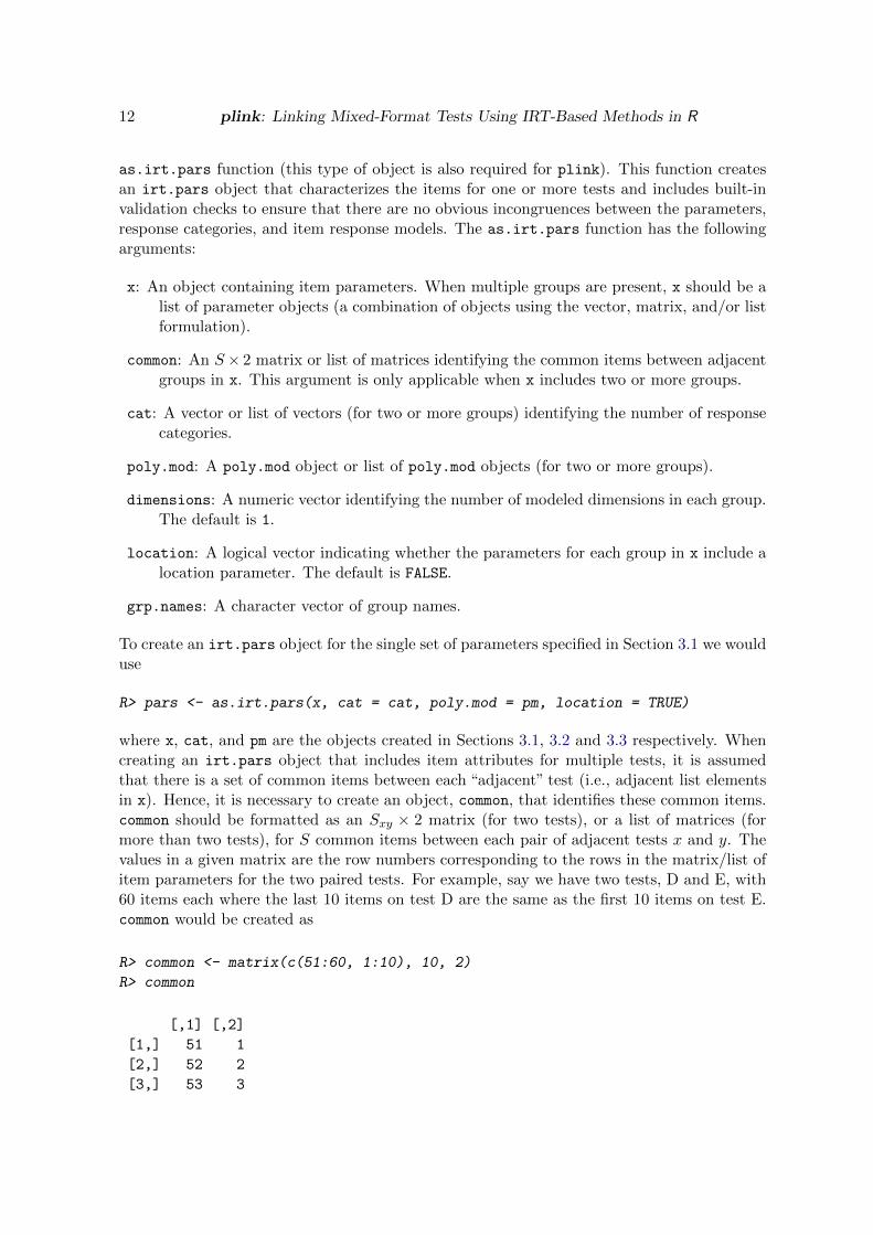
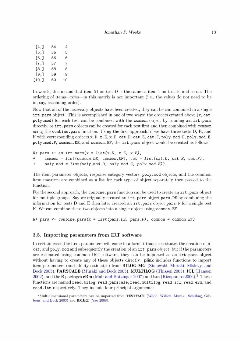
where x, cat, and pm are the objects created in Sections 3.1, 3.2 and 3.3 respectively. Whencreating an irt.pars object that includes item attributes for multiple tests, it is assumedthat there is a set of common items between each “adjacent” test (i.e., adjacent list elementsin x). Hence, it is necessary to create an object, common, that identifies these common items.common should be formatted as an Sxy × 2 matrix (for two tests), or a list of matrices (formore than two tests), for S common items between each pair of adjacent tests x and y. Thevalues in a given matrix are the row numbers corresponding to the rows in the matrix/list ofitem parameters for the two paired tests. For example, say we have two tests, D and E, with60 items each where the last 10 items on test D are the same as the first 10 items on test E.common would be created as
R> common <- matrix(c(51:60, 1:10), 10, 2)
R> common
[,1] [,2]
[1,] 51 1
[2,] 52 2
[3,] 53 3
Jonathan P. Weeks 13
[4,] 54 4
[5,] 55 5
[6,] 56 6
[7,] 57 7
[8,] 58 8
[9,] 59 9
[10,] 60 10
In words, this means that item 51 on test D is the same as item 1 on test E, and so on. Theordering of items—rows—in this matrix is not important (i.e., the values do not need to bein, say, ascending order).
Now that all of the necessary objects have been created, they can be can combined in a singleirt.pars object. This is accomplished in one of two ways: the objects created above (x, cat,poly.mod) for each test can be combined with the common object by running as.irt.pars
directly, or irt.pars objects can be created for each test first and then combined with common
using the combine.pars function. Using the first approach, if we have three tests D, E, andF with corresponding objects x.D, x.E, x.F, cat.D, cat.E, cat.F, poly.mod.D, poly.mod.E,poly.mod.F, common.DE, and common.EF, the irt.pars object would be created as follows
R> pars <- as.irt.pars(x = list(x.D, x.E, x.F),
+ common = list(common.DE, common.EF), cat = list(cat.D, cat.E, cat.F),
+ poly.mod = list(poly.mod.D, poly.mod.E, poly.mod.F))
The item parameter objects, response category vectors, poly.mod objects, and the commonitem matrices are combined as a list for each type of object separately then passed to thefunction.
For the second approach, the combine.pars function can be used to create an irt.pars objectfor multiple groups. Say we originally created an irt.pars object pars.DE by combining theinformation for tests D and E then later created an irt.pars object pars.F for a single testF. We can combine these two objects into a single object using common.EF.
R> pars <- combine.pars(x = list(pars.DE, pars.F), common = common.EF)
3.5. Importing parameters from IRT software
In certain cases the item parameters will come in a format that necessitates the creation of x,cat, and poly.mod and subsequently the creation of an irt.pars object, but if the parametersare estimated using common IRT software, they can be imported as an irt.pars objectwithout having to create any of these objects directly. plink includes functions to importitem parameters (and ability estimates) from BILOG-MG (Zimowski, Muraki, Mislevy, andBock 2003), PARSCALE (Muraki and Bock 2003), MULTILOG (Thissen 2003), ICL (Hanson2002), and the R packages eRm (Mair and Hatzinger 2007) and ltm (Rizopoulos 2006).2 Thesefunctions are named read.bilog, read.parscale, read.multilog, read.icl, read.erm, andread.ltm respectively. They include four principal arguments:
2Multidimensional parameters can be imported from TESTFACT (Wood, Wilson, Muraki, Schilling, Gib-bons, and Bock 2003) and BMIRT (Yao 2008).
14 plink: Linking Mixed-Format Tests Using IRT-Based Methods in R
file: The filename of the file containing the item or ability parameters.
ability: A logical value indicating whether the file contains ability parameters. The defaultis FALSE.
loc.out: A logical value indicating whether threshold/step parameters should be formattedas deviations from a location parameter (not applicable for read.bilog). The defaultis FALSE.
as.irt.pars: A logical value indicating whether the item parameters should be importedas an irt.pars object. The default is TRUE.
In addition to the four arguments above, there are other function-specific arguments. Forinstance, with read.erm and read.ltm, there is no file argument because the output iscreated in R. The main argument in these functions, x, is the output object from one ofthe following functions in eRm: RM, RSM, PCM, LLTM, RSM, or PCM; or from ltm:3 rasch,ltm, tpm, grm, or gpcm. For the read.icl function, a poly.mod object must be createdbecause no information about the item type is included in the .par file, and for the functionsread.bilog and read.parscale a logical argument, pars.only, can be included to indicatewhether information like standard errors should be included with the returned parameters.
Relative to the other applications, MULTILOG has the greatest flexibility for specifying itemresponse models, yet the information in the .par file provides minimal information aboutthe model(s) and the associated constraints (the .par file only includes contrast parameters).As such, for read.multilog, it is necessary to create both a cat and poly.mod object, anddepending on the specified model(s), it may be necessary to include the arguments drm.3PL
and/or contrast. drm.3PL is a logical argument indicating whether the 3PL was used tomodel the dichotomous items (the default is TRUE). The contrast argument is a bit morecomplex. With the exception of the 1PL, 2PL, and GRM, all of the models in MULTILOGare constrained versions of the multiple-choice model where various contrast parameters areestimated (see Thissen and Steinberg 1986). These can include deviation, polynomial, ortriangular contrasts for individual parameters on specific items. The contrast argumentis used to identify these constraints. A full explanation of this argument, in addition toinformation on importing parameters from the other software packages, is included in thedocumentation in plink.
4. Running the calibration
Once an irt.pars object with two or more tests has been created, the function plink canbe used to estimate linking constants and (if desired) transform all of the item and/or abilityparameters onto a base scale. The function includes one essential argument x, and twelveoptional arguments.4 These arguments are presented in the context of several examples.
x: An irt.pars object with two or more groups.
3plink and ltm both have functions named grm and gpcm. With both packages running, it may be necessaryto call the appropriate function using plink::grm, plink::gpcm, ltm::grm, or ltm::gpcm
4There are two additional arguments, dilation and dim.order, that only pertain to multidimensionallinking methods.
Jonathan P. Weeks 15
rescale: A character value identifying the linking constants to use to transform the pa-rameters to the base scale. Applicable values are “MS”, “MM”, “HB”, and “SL” for themean/sigma, mean/mean, Haebara, and Stocking-Lord methods respectively.
ability: A list of θ values where the number of list elements equals the number of groupsin x.
method: A character vector identifying the method(s) to use when estimating the linking con-stants. Applicable values are “MS”, “MM”, “HB”, and “SL”. If missing, linking constantswill be estimated using all four methods.
weights.t: A list containing quadrature points and weights on the to scale for use with thecharacteristic curve methods.
weights.f: A list containing quadrature points and weights on the from scale for use withthe characteristic curve methods. This argument will be ignored if symmetric = FALSE.
startvals: A vector of starting values for A and B respectively for use in the characteristiccurve methods or a character value equal to “MS” or “MM” indicating that estimatesfrom the given moment method should be used. If the argument is missing, values fromthe mean/sigma method are used.
exclude: A character vector or list identifying common items that should be excluded whenestimating the linking constants.
score: An integeridentifying the scoring function to use for the Stocking-Lord method.When score = 1, the ordered categories for each item are scored from 0 to k − 1, andwhen score = 2, the categories are scored from 1 to k. The default is 1. A vector ofscores for each response category can also be supplied, but this is only recommendedfor advanced users.
base.grp: An integer identifying the reference scale—base group—onto which all item andability parameters should be placed. The default is 1.
symmetric: A logical value indicating whether symmetric optimization should be used forthe characteristic curve methods. The default is FALSE.
rescale.com: A logical value. If TRUE, rescale the common item parameters using theestimated linking constants; otherwise, insert the non-transformed common item pa-rameters into the set of unique transformed item parameters. The default is TRUE.
grp.names: A character vector of names for each group in x (i.e., names for each test).If group names are identified when creating the irt.pars object, this argument isunnecessary.
...: Further arguments passed to other methods.
4.1. Two groups, dichotomous data
The simplest linking scenario is the case where there are only two tests and all of the items(unique and common) are dichotomously scored. This example uses the KB04 dataset which

16 plink: Linking Mixed-Format Tests Using IRT-Based Methods in R
reproduces the data presented by Kolen and Brennan (2004) in Table 6.5 (p. 192). There are36 items on each test with 12 common items between them. The KB04 dataset is formatted as alist with two elements. The first element is a list of length two containing the item parametersfor “new” and ”old” forms respectively, and the second element is a matrix identifying thecommon items between the two tests. These elements correspond to the objects x and common,but cat and poly.mod still need to be created. The following code is used to create theseobjects and the combined irt.pars object
R> cat <- rep(2, 36)
R> pm <- as.poly.mod(36)
R> x <- as.irt.pars(KB04$pars, KB04$common, cat = list(cat, cat),
+ poly.mod = list(pm, pm), grp.names = c("new", "old"))
Once this object is created, plink can be run without specifying any additional arguments.
R> out <- plink(x)
R> summary(out)
------- old/new* -------
Linking Constants
A B
Mean/Mean 0.821513 0.457711
Mean/Sigma 0.855511 0.441053
Haebara 0.907748 0.408260
Stocking-Lord 0.900655 0.425961
There are two things to notice in this output. First, no method argument was specified, solinking constants were estimated using all four approaches, and second, there is an asteriskincluded next to the group name “new” indicating that this is the base group (this will be ofparticular importance in the examples with more than two groups). Although not obvious inthis example, no rescaled parameters are returned. To return the rescaled item parameters,the rescale argument must be included. More than one method can be used to estimate thelinking constants, but parameters can only be rescaled using a single approach, meaning onlyone method can be specified for rescale.
In the following example, the parameters are rescaled using the Stocking-Lord method withthe “old” form (i.e., the second set of parameters in x) treated as the base scale.
R> out <- plink(x, rescale = "SL", base.grp = 2)
R> summary(out)
------- new/old* -------
Linking Constants
A B
Mean/Mean 1.217266 -0.557155
Mean/Sigma 1.168892 -0.515543
Haebara 1.112133 -0.465667
Stocking-Lord 1.119231 -0.485545
Jonathan P. Weeks 17
The function link.pars can be used to extract the rescaled parameters (the only argumentis the output object from plink). These parameters are returned as an irt.pars object.Similarly, the function link.con can be used to extract the linking constants.
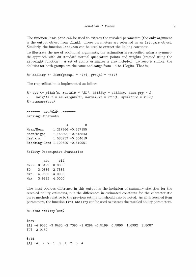
To illustrate the use of additional arguments, the estimation is respecified using a symmet-ric approach with 30 standard normal quadrature points and weights (created using theas.weight function). A set of ability estimates is also included. To keep it simple, theabilities for both groups are the same and range from −4 to 4 logits. That is,
R> ability <- list(group1 = -4:4, group2 = -4:4)
The respecification is implemented as follows
R> out <- plink(x, rescale = "SL", ability = ability, base.grp = 2,
+ weights.t = as.weight(30, normal.wt = TRUE), symmetric = TRUE)
R> summary(out)
------- new/old* -------
Linking Constants
A B
Mean/Mean 1.217266 -0.557155
Mean/Sigma 1.168892 -0.515543
Haebara 1.088233 -0.504619
Stocking-Lord 1.109529 -0.519901
Ability Descriptive Statistics
new old
Mean -0.5199 0.0000
SD 3.0386 2.7386
Min -4.9580 -4.0000
Max 3.9182 4.0000
The most obvious difference in this output is the inclusion of summary statistics for therescaled ability estimates, but the differences in estimated constants for the characteristiccurve methods relative to the previous estimation should also be noted. As with rescaled itemparameters, the function link.ability can be used to extract the rescaled ability parameters.
R> link.ability(out)
$new
[1] -4.9580 -3.8485 -2.7390 -1.6294 -0.5199 0.5896 1.6992 2.8087
[9] 3.9182
$old
[1] -4 -3 -2 -1 0 1 2 3 4
18 plink: Linking Mixed-Format Tests Using IRT-Based Methods in R
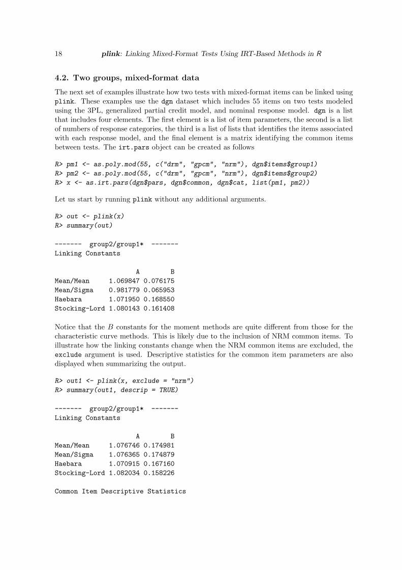
4.2. Two groups, mixed-format data
The next set of examples illustrate how two tests with mixed-format items can be linked usingplink. These examples use the dgn dataset which includes 55 items on two tests modeledusing the 3PL, generalized partial credit model, and nominal response model. dgn is a listthat includes four elements. The first element is a list of item parameters, the second is a listof numbers of response categories, the third is a list of lists that identifies the items associatedwith each response model, and the final element is a matrix identifying the common itemsbetween tests. The irt.pars object can be created as follows
R> pm1 <- as.poly.mod(55, c("drm", "gpcm", "nrm"), dgn$items$group1)
R> pm2 <- as.poly.mod(55, c("drm", "gpcm", "nrm"), dgn$items$group2)
R> x <- as.irt.pars(dgn$pars, dgn$common, dgn$cat, list(pm1, pm2))
Let us start by running plink without any additional arguments.
R> out <- plink(x)
R> summary(out)
------- group2/group1* -------
Linking Constants
A B
Mean/Mean 1.069847 0.076175
Mean/Sigma 0.981779 0.065953
Haebara 1.071950 0.168550
Stocking-Lord 1.080143 0.161408
Notice that the B constants for the moment methods are quite different from those for thecharacteristic curve methods. This is likely due to the inclusion of NRM common items. Toillustrate how the linking constants change when the NRM common items are excluded, theexclude argument is used. Descriptive statistics for the common item parameters are alsodisplayed when summarizing the output.
R> out1 <- plink(x, exclude = "nrm")
R> summary(out1, descrip = TRUE)
------- group2/group1* -------
Linking Constants
A B
Mean/Mean 1.076746 0.174981
Mean/Sigma 1.076365 0.174879
Haebara 1.070915 0.167160
Stocking-Lord 1.082034 0.158226
Common Item Descriptive Statistics

Jonathan P. Weeks 19
Model: 3PL
Number of Items: 7
a b c
N Pars: 7.000000 7.000000 7.000000
Mean: To 0.955429 -0.304286 0.192286
Mean: From 1.028714 -0.443857 0.188857
SD: To 0.091653 1.025097 0.065622
SD: From 0.098714 0.952583 0.076230
Model: Generalized Partial Credit Model
Number of Items: 3
a b
N Pars: 3.000000 12.000000
Mean: To 1.097667 -0.002167
Mean: From 1.182000 -0.165250
SD: To 0.094813 1.114006
SD: From 0.101853 1.035063
Model: All
Number of Items: 10
a b c
N Pars: 10.000000 19.000000 7.000000
Mean: To 0.998100 -0.113474 0.192286
Mean: From 1.074700 -0.267895 0.188857
SD: To 0.113251 1.091870 0.065622
SD: From 0.121933 1.014405 0.076230
4.3. Six groups, mixed-format data
In the final example, the reading dataset is used to illustrate how the parameters frommultiple mixed-format tests can be chain-linked together using plink. For these data thereare six tests that span four grades and three years (see Table 1). The adjacent groups followa stair-step pattern (e.g., the grade 3 and grade 4 tests in year 0 are linked then the grade 4tests in years 0 and 1 are linked, etc.) As with dgn, the object reading includes most of theelements needed to create the irt.pars object, but it is still necessary to create the poly.modobjects for each test. The following code is used for this purpose.
R> pm1 <- as.poly.mod(41, c("drm", "gpcm"), reading$items[[1]])
R> pm2 <- as.poly.mod(70, c("drm", "gpcm"), reading$items[[2]])
R> pm3 <- as.poly.mod(70, c("drm", "gpcm"), reading$items[[3]])
R> pm4 <- as.poly.mod(70, c("drm", "gpcm"), reading$items[[4]])
R> pm5 <- as.poly.mod(72, c("drm", "gpcm"), reading$items[[5]])
R> pm6 <- as.poly.mod(71, c("drm", "gpcm"), reading$items[[6]])
R> pm <- list(pm1, pm2, pm3, pm4, pm5, pm6)
20 plink: Linking Mixed-Format Tests Using IRT-Based Methods in R
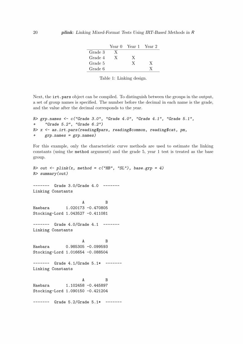
Year 0 Year 1 Year 2
Grade 3 XGrade 4 X XGrade 5 X XGrade 6 X
Table 1: Linking design.
Next, the irt.pars object can be compiled. To distinguish between the groups in the output,a set of group names is specified. The number before the decimal in each name is the grade,and the value after the decimal corresponds to the year.
R> grp.names <- c("Grade 3.0", "Grade 4.0", "Grade 4.1", "Grade 5.1",
+ "Grade 5.2", "Grade 6.2")
R> x <- as.irt.pars(reading$pars, reading$common, reading$cat, pm,
+ grp.names = grp.names)
For this example, only the characteristic curve methods are used to estimate the linkingconstants (using the method argument) and the grade 5, year 1 test is treated as the basegroup.
R> out <- plink(x, method = c("HB", "SL"), base.grp = 4)
R> summary(out)
------- Grade 3.0/Grade 4.0 -------
Linking Constants
A B
Haebara 1.020173 -0.470805
Stocking-Lord 1.043527 -0.411081
------- Grade 4.0/Grade 4.1 -------
Linking Constants
A B
Haebara 0.985305 -0.099593
Stocking-Lord 1.016654 -0.088504
------- Grade 4.1/Grade 5.1* -------
Linking Constants
A B
Haebara 1.102458 -0.445897
Stocking-Lord 1.090150 -0.421204
------- Grade 5.2/Grade 5.1* -------
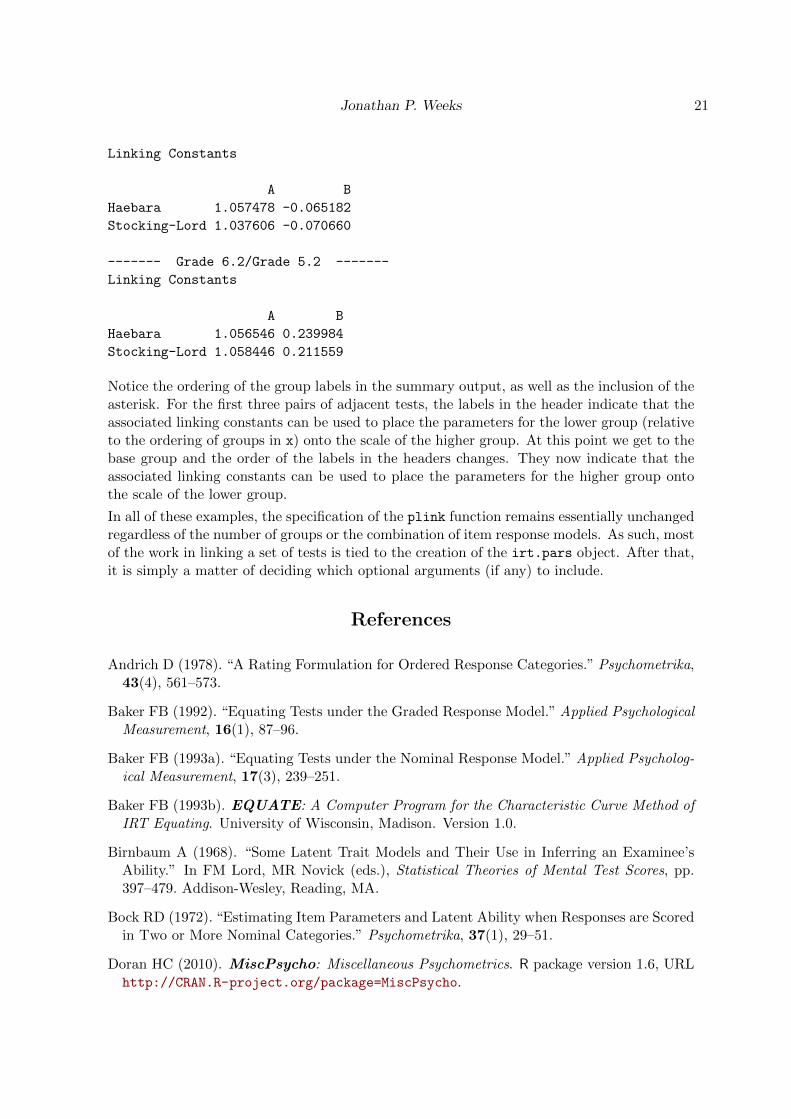
Jonathan P. Weeks 21
Linking Constants
A B
Haebara 1.057478 -0.065182
Stocking-Lord 1.037606 -0.070660
------- Grade 6.2/Grade 5.2 -------
Linking Constants
A B
Haebara 1.056546 0.239984
Stocking-Lord 1.058446 0.211559
Notice the ordering of the group labels in the summary output, as well as the inclusion of theasterisk. For the first three pairs of adjacent tests, the labels in the header indicate that theassociated linking constants can be used to place the parameters for the lower group (relativeto the ordering of groups in x) onto the scale of the higher group. At this point we get to thebase group and the order of the labels in the headers changes. They now indicate that theassociated linking constants can be used to place the parameters for the higher group ontothe scale of the lower group.
In all of these examples, the specification of the plink function remains essentially unchangedregardless of the number of groups or the combination of item response models. As such, mostof the work in linking a set of tests is tied to the creation of the irt.pars object. After that,it is simply a matter of deciding which optional arguments (if any) to include.
References
Andrich D (1978). “A Rating Formulation for Ordered Response Categories.” Psychometrika,43(4), 561–573.
Baker FB (1992). “Equating Tests under the Graded Response Model.” Applied PsychologicalMeasurement, 16(1), 87–96.
Baker FB (1993a). “Equating Tests under the Nominal Response Model.” Applied Psycholog-ical Measurement, 17(3), 239–251.
Baker FB (1993b). EQUATE: A Computer Program for the Characteristic Curve Method ofIRT Equating. University of Wisconsin, Madison. Version 1.0.
Birnbaum A (1968). “Some Latent Trait Models and Their Use in Inferring an Examinee’sAbility.” In FM Lord, MR Novick (eds.), Statistical Theories of Mental Test Scores, pp.397–479. Addison-Wesley, Reading, MA.
Bock RD (1972). “Estimating Item Parameters and Latent Ability when Responses are Scoredin Two or More Nominal Categories.” Psychometrika, 37(1), 29–51.
Doran HC (2010). MiscPsycho: Miscellaneous Psychometrics. R package version 1.6, URLhttp://CRAN.R-project.org/package=MiscPsycho.

22 plink: Linking Mixed-Format Tests Using IRT-Based Methods in R
Gulliksen H (1950). Theory of Mental Tests. John Wiley & Sons, New York.
Haebara T (1980). “Equating Logistic Ability Scales by a Weighted Least Squares Method.”Japanese Psychological Research, 22(3), 144–149.
Han KT (2007). IRTEQ: Windows Application that Implements IRT Scaling and Equating.University of Massachusetts, Amherst. Version 1.0, URL http://www.umass.edu/remp/
software/irteq/.
Han KT, Hambelton RK (2007). WinGen2: Windows Software that Generates IRT ModelParameters and Item Responses. University of Massachusetts, Amherst. Version 1.0, URLhttp://www.umass.edu/remp/software/wingen/.
Hanson BA (2000). mcmequate: Equating Software for the Multiple-Choice Model. Ver-sion 1.0, URL http://www.b-a-h.com/software/mcmequate/index.html.
Hanson BA (2002). IRT Command Language. Version 1.0, URL http://www.b-a-h.
com/software/irt/icl/.
Hanson BA, Zeng L (1995). ST: A Computer Program for IRT Scale Transformation. Uni-versity of Iowa. Version 1.0, URL http://www.education.uiowa.edu/casma/computer_
programs.htm#irt.
Hull CL (1922). “The Conversion of Test Scores Into Series Which Shall Have Any AssignedMean and Degree of Dispersion.” Journal of Applied Psychology, 6(4), 298–300.
Kelley TL (1923). Statistical Method. Macmillan, New York.
Kim J, Hanson BA (2002). “Test Equating under the Multiple-Choice Model.” AppliedPsychological Measurement, 26(3), 255–270.
Kim S, Kolen MJ (2003). POLYST: A Computer Program for Polytomous IRT Scale Trans-formation. University of Iowa. Version 1.0, URL http://www.education.uiowa.edu/
casma/computer_programs.htm#irt.
Kim S, Kolen MJ (2004). STUIRT: A Computer Program for Scale Transformation underUnidimensional Item Response Theory Models. University of Iowa. Version 1.0, URLhttp://www.education.uiowa.edu/casma/computer_programs.htm#irt.
Kim S, Lee W (2006). “An Extension of Four IRT Linking Methods for Mixed-Format Tests.”Journal of Educational Measurement, 43(1), 53–76.
Kolen MJ (1981). “Comparison of Traditional and Item Response Theory Methods for Equat-ing Tests.” Journal of Educational Measurement, 18(1), 1–11.
Kolen MJ (2004). POLYEQUATE. University of Iowa. Version 1.0, URL http://www.
education.uiowa.edu/casma/computer_programs.htm#irt.
Kolen MJ, Brennan RL (2004). Test Equating, Scaling, and Linking: Methods and Practices.2nd edition. Springer-Verlag, New York.
Lee K, Oshima TC (1997). Iplink: Item Parameter Linking. Version 2.0, URL http:
//education.gsu.edu/eps/4493.html.
Jonathan P. Weeks 23
Levine RE (1955). “Equating the Score Scales of Alternative Forms Administered to Samplesof Different Ability.” Research Bulletin 55-23, Educational Testing Services, Princeton, NJ.
Linn RL (1993). “Linking Results of Distinct Assessments.” Applied Measurement in Educa-tion, 6(1), 83–102.
Linn RL, Levine MV, Hastings CN, Wardrop JL (1980). “An Investigation of Item Bias in aTest of Reading Comprehension.” Technical Report 163, University of Illinois, Center forthe Study of Reading, Urbana, IL.
Lord FM (1952). “A Theory of Test Scores.” Psychometric Monographs. No. 7.
Lord FM (1980). Applications of Item Response Theory to Practical Testing Problems.Lawrence Erlbaum Associates, Hillsdale, NJ.
Lord FM, Novick MR (1968). Statistical Theories of Mental Test Scores. Addison-Wesley,Reading, MA.
Loyd BH, Hoover HD (1980). “Vertical Equating Using the Rasch Model.” Journal of Edu-cational Measurement, 17(3), 179–193.
Mair P, Hatzinger R (2007). “Extended Rasch Modeling: The eRm Package for the Ap-plication of IRT Models in R.” Journal of Statistical Software, 20(9), 1–20. URLhttp://www.jstatsoft.org/v20/i09/.
Marco GL (1977). “Item Characteristic Curve Solutions to Three Intractable Testing Prob-lems.” Journal of Educational Measurement, 14(2), 139–160.
Masters GN (1982). “A Rasch Model for Partial Credit Scoring.” Psychometrika, 47(2),149–174.
Muraki E (1992). “A Generalized Partial Credit Model: Application of an EM Algorithm.”Applied Psychological Measurement, 16(2), 159–176.
Muraki E, Bock RD (2003). PARSCALE 4: IRT Item Analysis and Test Scoring forRating-Scale Data. Scientific Software International, Inc., Lincolnwood, IL. Version 4.0,URL http://www.ssicentral.com/.
Partchev I (2009). irtoys: Simple Interface to the Estimation and Plotting of IRT Models.R package version 0.1.2, URL http://CRAN.R-project.org/package=irtoys.
Petersen NS, Cook LL, Stocking ML (1983). “IRT Versus Conventional Equating Methods:A Comparative Study of Scale Stability.” Journal of Educational Statistics, 8(2), 137–156.
Rasch G (1960). Probabilistic Models for Some Intelligence and Attainment Tests. DanishInstitute for Educational Research, Copenhagen, Denmark.
R Development Core Team (2010). R: A Language and Environment for Statistical Computing.R Foundation for Statistical Computing, Vienna, Austria. ISBN 3-900051-07-0, URL http:
//www.R-project.org/.
24 plink: Linking Mixed-Format Tests Using IRT-Based Methods in R
Rizopoulos D (2006). “ltm: An R Package for Latent Variable Modeling and Item Re-sponse Theory Analyses.” Journal of Statistical Software, 17(5), 1–25. URL http:
//www.jstatsoft.org/v17/i05/.
Samejima F (1969). “Estimation of Latent Ability Using a Response Pattern of GradedScores.” Psychometric Monograph Supplement, 4(34).
Samejima F (1979). “A New Family of Models for the Multiple Choice Item.” Research Report79-4, University of Tennessee, Department of Psychology, Knoxville, TN.
Sarkar D (2008). lattice: Multivariate Data Visualization with R. Springer-Verlag, New York.
Stocking ML, Lord FM (1983). “Developing a Common Metric in Item Response Theory.”Applied Psychological Measurement, 7(2), 201–210.
Thissen D (2003). MULTILOG 7: Multiple, Categorical Item Analysis and Test ScoringUsing Item Response Theory. Scientific Software International Inc., Lincolnwood, IL. Ver-sion 7.0, URL http://www.ssicentral.com/.
Thissen D, Steinberg L (1984). “A Response Model for Multiple Choice Items.”Psychometrika,49(4), 501–519.
Thissen D, Steinberg L (1986). “A Taxonomy of Item Response Models.” Psychometrika,51(4), 567–577.
Thurstone LL (1925). “A Method of Scaling Psychological and Educational Tests.” Journalof Educational Psychology, 16(7), 433–451.
Thurstone LL (1938). “Primary Mental Abilities.” Psychometric Monographs. No. 1.
Weeks JP (2010). “plink: An R Package for Linking Mixed-Format Tests Using IRT-BasedMethods.” Journal of Statistical Software, 35(12), 1–33. URL http://www.jstatsoft.
org/v35/i12/.
Wood R, Wilson DT, Muraki E, Schilling SG, Gibbons R, Bock RD (2003). TESTFACT 4:Test Scoring, Item Statistics, and Item Factor Analysis. Scientific Software InternationalInc., Lincolnwood, IL. Version 4.0, URL http://www.ssicentral.com/.
Yao L (2008). BMIRT: Bayesian Multivariate Item Response Theory. CTB/McGraw-Hill,Monterey, CA. Version 1.0.
Yen WM (1986). “The Choice of Scale for Educational Measurement: An IRT Perspective.”Journal of Educational Measurement, 23(4), 299–325.
Zimowski MF, Muraki E, Mislevy RJ, Bock RD (2003). BILOG–MG 3: Multiple-GroupIRT Analysis and Test Maintenance for Binary Items. Scientific Software InternationalInc., Lincolnwood, IL. Version 3.0, URL http://www.ssicentral.com/.
Jonathan P. Weeks 25
A. Additional features
The primary purpose of plink is to facilitate the linking of tests using IRT-based methods;however, there are three other notable features of the package. plink can be used to computeresponse probabilities, conduct IRT true-score and observed-score equating (Kolen and Bren-nan 2004), and plot item response curves and comparison plots for examining item parameterdrift.
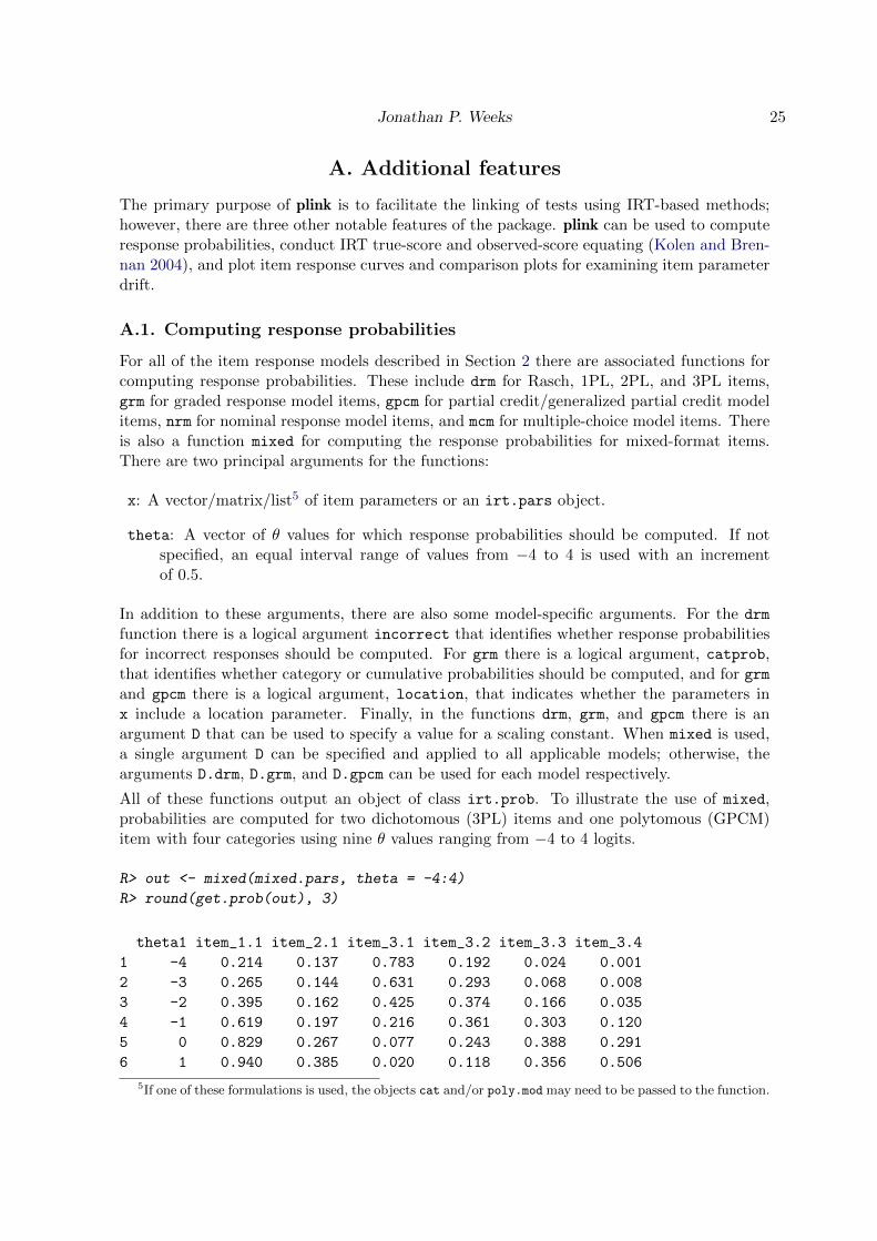
A.1. Computing response probabilities
For all of the item response models described in Section 2 there are associated functions forcomputing response probabilities. These include drm for Rasch, 1PL, 2PL, and 3PL items,grm for graded response model items, gpcm for partial credit/generalized partial credit modelitems, nrm for nominal response model items, and mcm for multiple-choice model items. Thereis also a function mixed for computing the response probabilities for mixed-format items.There are two principal arguments for the functions:
x: A vector/matrix/list5 of item parameters or an irt.pars object.
theta: A vector of θ values for which response probabilities should be computed. If notspecified, an equal interval range of values from −4 to 4 is used with an incrementof 0.5.
In addition to these arguments, there are also some model-specific arguments. For the drm
function there is a logical argument incorrect that identifies whether response probabilitiesfor incorrect responses should be computed. For grm there is a logical argument, catprob,that identifies whether category or cumulative probabilities should be computed, and for grmand gpcm there is a logical argument, location, that indicates whether the parameters inx include a location parameter. Finally, in the functions drm, grm, and gpcm there is anargument D that can be used to specify a value for a scaling constant. When mixed is used,a single argument D can be specified and applied to all applicable models; otherwise, thearguments D.drm, D.grm, and D.gpcm can be used for each model respectively.
All of these functions output an object of class irt.prob. To illustrate the use of mixed,probabilities are computed for two dichotomous (3PL) items and one polytomous (GPCM)item with four categories using nine θ values ranging from −4 to 4 logits.
R> out <- mixed(mixed.pars, theta = -4:4)
R> round(get.prob(out), 3)
theta1 item_1.1 item_2.1 item_3.1 item_3.2 item_3.3 item_3.4
1 -4 0.214 0.137 0.783 0.192 0.024 0.001
2 -3 0.265 0.144 0.631 0.293 0.068 0.008
3 -2 0.395 0.162 0.425 0.374 0.166 0.035
4 -1 0.619 0.197 0.216 0.361 0.303 0.120
5 0 0.829 0.267 0.077 0.243 0.388 0.291
6 1 0.940 0.385 0.020 0.118 0.356 0.506
5If one of these formulations is used, the objects cat and/or poly.mod may need to be passed to the function.
26 plink: Linking Mixed-Format Tests Using IRT-Based Methods in R
7 2 0.981 0.548 0.004 0.045 0.257 0.694
8 3 0.994 0.715 0.001 0.015 0.161 0.823
9 4 0.998 0.844 0.000 0.005 0.093 0.902
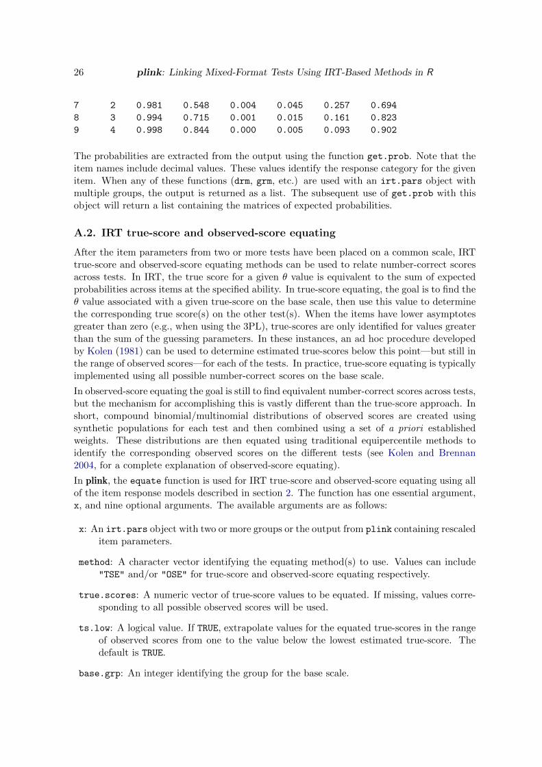
The probabilities are extracted from the output using the function get.prob. Note that theitem names include decimal values. These values identify the response category for the givenitem. When any of these functions (drm, grm, etc.) are used with an irt.pars object withmultiple groups, the output is returned as a list. The subsequent use of get.prob with thisobject will return a list containing the matrices of expected probabilities.
A.2. IRT true-score and observed-score equating
After the item parameters from two or more tests have been placed on a common scale, IRTtrue-score and observed-score equating methods can be used to relate number-correct scoresacross tests. In IRT, the true score for a given θ value is equivalent to the sum of expectedprobabilities across items at the specified ability. In true-score equating, the goal is to find theθ value associated with a given true-score on the base scale, then use this value to determinethe corresponding true score(s) on the other test(s). When the items have lower asymptotesgreater than zero (e.g., when using the 3PL), true-scores are only identified for values greaterthan the sum of the guessing parameters. In these instances, an ad hoc procedure developedby Kolen (1981) can be used to determine estimated true-scores below this point—but still inthe range of observed scores—for each of the tests. In practice, true-score equating is typicallyimplemented using all possible number-correct scores on the base scale.
In observed-score equating the goal is still to find equivalent number-correct scores across tests,but the mechanism for accomplishing this is vastly different than the true-score approach. Inshort, compound binomial/multinomial distributions of observed scores are created usingsynthetic populations for each test and then combined using a set of a priori establishedweights. These distributions are then equated using traditional equipercentile methods toidentify the corresponding observed scores on the different tests (see Kolen and Brennan2004, for a complete explanation of observed-score equating).
In plink, the equate function is used for IRT true-score and observed-score equating using allof the item response models described in section 2. The function has one essential argument,x, and nine optional arguments. The available arguments are as follows:
x: An irt.pars object with two or more groups or the output from plink containing rescaleditem parameters.
method: A character vector identifying the equating method(s) to use. Values can include"TSE" and/or "OSE" for true-score and observed-score equating respectively.
true.scores: A numeric vector of true-score values to be equated. If missing, values corre-sponding to all possible observed scores will be used.
ts.low: A logical value. If TRUE, extrapolate values for the equated true-scores in the rangeof observed scores from one to the value below the lowest estimated true-score. Thedefault is TRUE.
base.grp: An integer identifying the group for the base scale.
Jonathan P. Weeks 27
score: An integer identifying the scoring function to use to compute the true-scores. Whenscore = 1, the ordered categories for each item are scored from 0 to k − 1, and whenscore = 2, the categories are scored from 1 to k. The default is 1.
startval: An integer starting value for the first value of true.score.
weights1: A list containing quadrature points and weights to be used in the observed-scoreequating for population 1.
weights2: A list containing quadrature points and weights to be used in the observed-scoreequating for population 2.
syn.weights: A vector of length two or a list containing vectors of length two with syntheticpopulation weights to be used for each pair of tests for populations 1 and 2 respectivelyfor observed-score equating. If missing, weights of 0.5 will be used for both populationsfor all groups. If syn.weights is a list, the number of list elements should be equal tothe number of groups in x minus one.
...: Further arguments passed to or from other methods.
As an illustration of the equate function, the example presented in (Kolen and Brennan 2004,pp. 191-198) is recreated using the dichotomous item parameters from the KB04 dataset. Asa first step, the forms are linked using the mean/sigma method, excluding item 27, with the“old” test as the base scale and the scaling constant, D, equal to 1.7.
R> pm <- as.poly.mod(36)
R> x <- as.irt.pars(KB04$pars, KB04$common,
+ cat = list(rep(2, 36), rep(2, 36)), poly.mod = list(pm, pm))
R> out <- plink(x, rescale = "MS", base.grp = 2, D = 1.7,
+ exclude = list(27, 27), grp.names = c("new", "old"))
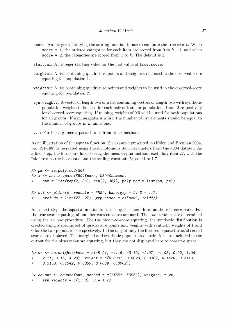
As a next step, the equate function is run using the “new” form as the reference scale. Forthe true-score equating, all number-correct scores are used. The lowest values are determinedusing the ad hoc procedure. For the observed-score equating, the synthetic distribution iscreated using a specific set of quadrature points and weights with synthetic weights of 1 and0 for the two populations respectively. In the output only the first ten equated true/observedscores are displayed. The marginal and synthetic population distributions are included in theoutput for the observed-score equating, but they are not displayed here to conserve space.
R> wt <- as.weight(theta = c(-5.21, -4.16, -3.12, -2.07, -1.03, 0.02, 1.06,
+ 2.11, 3.15, 4.20), weight = c(0.0001, 0.0028, 0.0302, 0.1420, 0.3149,
+ 0.3158, 0.1542, 0.0359, 0.0039, 0.0002))
R> eq.out <- equate(out, method = c("TSE", "OSE"), weights1 = wt,
+ syn.weights = c(1, 0), D = 1.7)
28 plink: Linking Mixed-Format Tests Using IRT-Based Methods in R
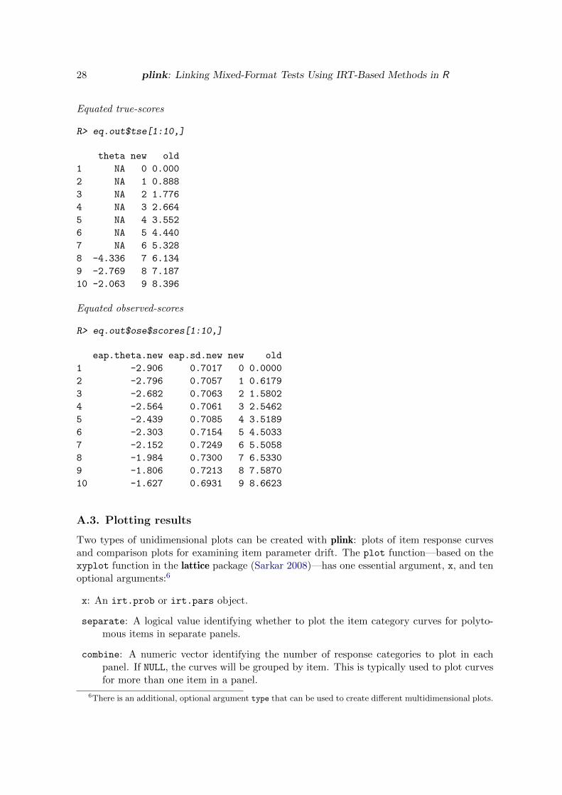
Equated true-scores
R> eq.out$tse[1:10,]
theta new old
1 NA 0 0.000
2 NA 1 0.888
3 NA 2 1.776
4 NA 3 2.664
5 NA 4 3.552
6 NA 5 4.440
7 NA 6 5.328
8 -4.336 7 6.134
9 -2.769 8 7.187
10 -2.063 9 8.396
Equated observed-scores
R> eq.out$ose$scores[1:10,]
eap.theta.new eap.sd.new new old
1 -2.906 0.7017 0 0.0000
2 -2.796 0.7057 1 0.6179
3 -2.682 0.7063 2 1.5802
4 -2.564 0.7061 3 2.5462
5 -2.439 0.7085 4 3.5189
6 -2.303 0.7154 5 4.5033
7 -2.152 0.7249 6 5.5058
8 -1.984 0.7300 7 6.5330
9 -1.806 0.7213 8 7.5870
10 -1.627 0.6931 9 8.6623
A.3. Plotting results
Two types of unidimensional plots can be created with plink: plots of item response curvesand comparison plots for examining item parameter drift. The plot function—based on thexyplot function in the lattice package (Sarkar 2008)—has one essential argument, x, and tenoptional arguments:6
x: An irt.prob or irt.pars object.
separate: A logical value identifying whether to plot the item category curves for polyto-mous items in separate panels.
combine: A numeric vector identifying the number of response categories to plot in eachpanel. If NULL, the curves will be grouped by item. This is typically used to plot curvesfor more than one item in a panel.
6There is an additional, optional argument type that can be used to create different multidimensional plots.
Jonathan P. Weeks 29
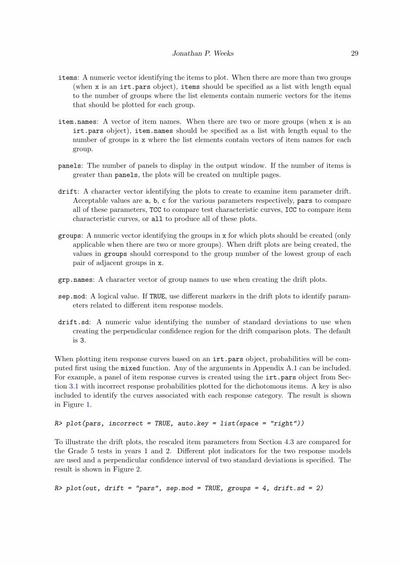
items: A numeric vector identifying the items to plot. When there are more than two groups(when x is an irt.pars object), items should be specified as a list with length equalto the number of groups where the list elements contain numeric vectors for the itemsthat should be plotted for each group.
item.names: A vector of item names. When there are two or more groups (when x is anirt.pars object), item.names should be specified as a list with length equal to thenumber of groups in x where the list elements contain vectors of item names for eachgroup.
panels: The number of panels to display in the output window. If the number of items isgreater than panels, the plots will be created on multiple pages.
drift: A character vector identifying the plots to create to examine item parameter drift.Acceptable values are a, b, c for the various parameters respectively, pars to compareall of these parameters, TCC to compare test characteristic curves, ICC to compare itemcharacteristic curves, or all to produce all of these plots.
groups: A numeric vector identifying the groups in x for which plots should be created (onlyapplicable when there are two or more groups). When drift plots are being created, thevalues in groups should correspond to the group number of the lowest group of eachpair of adjacent groups in x.
grp.names: A character vector of group names to use when creating the drift plots.
sep.mod: A logical value. If TRUE, use different markers in the drift plots to identify param-eters related to different item response models.
drift.sd: A numeric value identifying the number of standard deviations to use whencreating the perpendicular confidence region for the drift comparison plots. The defaultis 3.
When plotting item response curves based on an irt.pars object, probabilities will be com-puted first using the mixed function. Any of the arguments in Appendix A.1 can be included.For example, a panel of item response curves is created using the irt.pars object from Sec-tion 3.1 with incorrect response probabilities plotted for the dichotomous items. A key is alsoincluded to identify the curves associated with each response category. The result is shownin Figure 1.
R> plot(pars, incorrect = TRUE, auto.key = list(space = "right"))
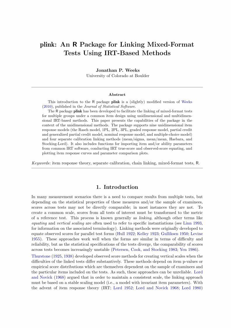
To illustrate the drift plots, the rescaled item parameters from Section 4.3 are compared forthe Grade 5 tests in years 1 and 2. Different plot indicators for the two response modelsare used and a perpendicular confidence interval of two standard deviations is specified. Theresult is shown in Figure 2.
R> plot(out, drift = "pars", sep.mod = TRUE, groups = 4, drift.sd = 2)

30 plink: Linking Mixed-Format Tests Using IRT-Based Methods in R
θ
Pro
babi
lity
0.0
0.2
0.4
0.6
0.8
1.0Item 1
−4 −2 0 2 4
Item 2 Item 3
Item 4 Item 5
0.0
0.2
0.4
0.6
0.8
1.0Item 6
0.0
0.2
0.4
0.6
0.8
1.0
−4 −2 0 2 4
Item 7 Item 8
−4 −2 0 2 4
Item 9
12345
●
●
●
●
●
Figure 1: Item response curves.
Discrimination/Slope Parameters
Grade 5.1
Gra
de 5
.2
0.0
0.5
1.0
0.0 0.5 1.0
●
●
●
●
●
●●
●
●●
●
●
●●
●
●●
●
●
●
DRM GPCM●
Difficulty/Step Parameters
Grade 5.1
Gra
de 5
.2
−2
−1
0
1
−2 −1 0 1
●
●●
●
●
●
●
●
●
●
●
●●
●
●
●
●
●
●
●
DRM GPCM●
Lower Asymptote Parameters
Grade 5.1
Gra
de 5
.2
0.1
0.2
0.3
0.4
0.5
0.1 0.2 0.3 0.4 0.5
●
●
●
●
●
●
●
●
●
●
●
●
●
●
●
●
●
●
●
●
DRM ●
Figure 2: Common item parameter comparison.

Jonathan P. Weeks 31
B. Related software
There are a number of software applications currently available for conducting IRT-basedlinking; however, no formal comparison of these programs has ever been done. The followingsection provides an overview/critique of each of these applications then compares the esti-mated linking constants across programs for a set of mixed-format item parameters undervarious conditions (e.g., non-symmetric versus symmetric optimization and uniform versusnormal weights) to determine if there are any appreciable differences.
One of the earliest programs to see widespread use was EQUATE (Baker 1993b) although nowit is rarely used in practice. In the original version the program implemented the Stocking-Lord method for items modeled using the 1PL, 2PL, and 3PL. Two years later it was updatedto allow for use of the graded response and nominal response models (the NRM utilizes theHaebara method). The program only allows for uniform weights at fixed ability intervals anddoes not support mixed-format tests, but it does include functionality to transform item andability parameters using the estimated linking constants.
In the same year as the update to EQUATE, Hanson and Zeng (1995) released the programST for linking dichotomous items, implementing the mean/sigma, mean/mean, Haebara, andStocking-Lord methods. In addition to the inclusion of the moment methods, the programallows one to specify quadrature points and weights for the characteristic curve methods.Hanson (2000) also developed the program mcmequate for linking nominal response andmultiple-choice model items using the Haebara method, but unlike ST no weighting optionsare available.
Two years after the release of ST, Lee and Oshima (1997) released the program IpLink whichallows for both unidimensional and multidimensional linking of dichotomously scored itemsusing the mean/sigma and characteristic curve methods with some flexibility for specifyingquadrature points (the weights cannot be explicitly defined). Unlike the previous applications,IpLink has a graphical user interface (GUI). Still, the program does not appear to have beenused much in practice for unidimensional linking.
As an extension of these programs (excluding the multidimensional methods), Kim and Kolen(2003) developed POLYST for linking dichotomous and polytomous items. The programimplements the same four linking methods as ST for the 1PL, 2PL, 3PL, GRM, PCM/GPCM,NRM, and MCM, although the calibration can only be run for items corresponding to asingle model at a time. In addition to the inclusion of more polytomous models, POLYSTadded increased functionality over the previous applications by allowing for symmetric andnon-symmetric optimization with the characteristic curve methods and extensive options forweighting the response probabilities in the criterion function.
As a further extension of POLYST, Kim and Kolen (2004) developed the program STUIRT tohandle mixed-format tests. STUIRT also includes two additional features: the ability to checkfor local minima near the final solution of the characteristic curve methods and functionalityto create input files for use in POLYEQUATE (Kolen 2004) to conduct IRT true-score andobserved-score equating. In ST, mcmequate, IpLink, POLYST, and STUIRT there is nofunctionality for transforming item parameters or ability estimates using the estimated linkingconstants.
One of the more recently developed applications is IRTEQ (Han 2007). This program im-plements the same four linking methods as STUIRT in addition to the robust mean/sigmamethod (Linn, Levine, Hastings, and Wardrop 1980) for the same item response models with
32 plink: Linking Mixed-Format Tests Using IRT-Based Methods in R
the exception of the nominal response and multiple-choice models. There are fewer optionsfor weighting the response probabilities in the criterion function, and the program does notallow for symmetric optimization; however, the program does include functionality for rescal-ing item/ability parameters and conducting true-score equating. Two additional featuresof IRTEQ are the availability of a GUI—the program can still be run from a syntax file ifdesired—and the ability to create plots comparing the item parameters and test characteristiccurves.
Two R packages, irtoys (Partchev 2009) and MiscPsycho (Doran 2010), also implement variouslinking methods, but both packages only include functionality for dichotomous items. irtoysis essentially a recreation of ST and MiscPsycho only implements the Stocking-Lord method.
There are two shortcomings to all of these applications: formatting of the input files, with thepossible exception of the R packages, and functionality for linking multiple tests. The firstfive programs (not including IpLink) require the creation of control files that can be highlysensitive to formatting. For instance, including an extra carriage return, lowercase letter, etc.in the file may cause the program not to run at all. For IRTEQ, the issue relates specifically tohow the item parameters must be formatted; they must conform to the PARSCALE (Murakiand Bock 2003) or WinGen2 (Han and Hambelton 2007) output format. This is an addedhassle for individuals not using PARSCALE to estimate item parameters or WinGen2 togenerate item parameters. The R packages require the item parameters to be formatted as amatrix or list for irtoys and MiscPsycho respectively, but depending on how the parametersare formatted when brought into R, some reformatting may be required. As described earlier,plink was written to provide a fair amount of flexibility in the formatting of item parametersby allowing them to be specified as vectors, matrices, lists, or imported from common IRTestimation programs.
The second major shortcoming is that none of the above programs allow for chain linkingof item and/or ability parameters across multiple tests. In all of these applications, linkingconstants can only be estimated for two groups at a time, meaning multiple control files mustbe created to estimate each set of constants. Then, as a second step, item parameters and/orability estimates must be iteratively transformed using another application. One of the keygoals in developing plink was to overcome this limitation.
There are three features missing from plink that are available in other programs: the useof polygonal approximation and the ability to check for local minima with the characteristiccurve methods (as implemented in STUIRT), and the availability of the robust mean/sigmamethod (as implemented in IRTEQ). However, plink provides greater flexibility for format-ting and importing item parameters than any other program, it is the only program thatsupports chain-linking, and (although not addressed here) it includes extensive functionalityfor multidimensional test linking.
B.1. Comparing the applications
To examine the comparability of these applications and plink, linking constants were es-timated with each program using the mixed-format item parameters available in STUIRT(example 3). There are two groups of 20 items (all common) which include ten 3PL items,five graded response model items, and five nominal response model items. Since most of theapplications are unable to handle mixed-format tests, the item parameters were separatedinto five comparison groups: 3PL items only, GRM items only, NRM items only, 3PL+GRM

Jonathan P. Weeks 33
items, and 3PL+GRM+NRM items. Linking constants were estimated for each comparisongroup, when applicable, using all available methods in each application. For the characteris-tic curve methods, a combination of two additional options, when applicable, were specified:uniform versus normal weights and symmetric versus non-symmetric optimization.
There were no differences in the linking constants estimated using the moment methods,but one should not expect any given that estimates are based solely on means and standarddeviations. The only instance where differences might occur is with the mean/sigma methodif the denominator for the standard deviations is n − 1 versus n. ST has the option to useeither, but all other programs that implement this approach use n in the denominator. For thecharacteristic curve methods, all of the programs produced nearly identical results, and whendifferences did occur they were at or beyond the third decimal place. Since all of the programsprovide consistent estimates for the linking constants, the only distinguishing features are theavailability of options and ease of use.
Affiliation:
Jonathan WeeksSchool of EducationUniversity of Colorado at BoulderUCB 249Boulder, CO 80309, United States of AmericaE-mail: [email protected]


![[IRT] Item Response Theory - Survey Design · Title irt — Introduction to IRT models DescriptionRemarks and examplesReferencesAlso see Description Item response theory (IRT) is](https://img.pdfslide.us/doc/110x75/605f13066a7f910fdc25b6b6/irt-item-response-theory-survey-design-title-irt-a-introduction-to-irt-models.jpg)