Pledgability and Liquidity:

A New Monetarist Model of Financial

and Macroeconomic Activity∗

Venky Venkateswaran† Randall Wright‡

March 24, 2013

Abstract

When limited commitment hinders unsecured credit, assets help by serving as collat-eral. We study models where assets differ in pledgability —the extent to which theycan be used to secure loans —and hence liquidity. Although many previous analyses ofimperfect credit focus on producers, we emphasize consumers. Household debt limitsare determined by the cost households incur when assets are seized in the event ofdefault. The framework, which nests standard growth and asset-pricing theory, is cal-ibrated to analyze the effects of monetary policy and financial innovation. We showthat inflation can raise output, employment and investment, plus improve housing andstock markets. For the baseline calibration, optimal inflation is positive. Increases inpledgability can generate booms and busts in economic activity, but may still be goodfor welfare.

∗We thank Guido Menzio, Guillaume Rocheteau, Neil Wallace, Yu Zhu and Chao He for their input, aswell as participants in seminars or conference presentaions at Wisconsin, Columbia, USC, the 2012 SEDMeetings in Cyprus, and the 2012 FRB Chicago Conference on Money, Banking and Payments. Wrightthanks the National Science Foundation and the Ray Zemon Chair in Liquid Assets at the WisconsinSchool of Business for research support. We also thank the Toulouse School of Economics, where we beganthis project, for their hospitality. The usual disclaimers apply.†Pennsylvania State University (vuv10@psu.edu).‡University of Wisconsin-Madison, FRB Minneapolis, FRB Chicago and NBER (rwright@bus.wisc.edu).

Collateral is, after all, only good if a creditor can get his hands on it. NiallFerguson, The Ascent of Money.

1 Introduction

This project develops a theory of the role of assets in the exchange process and uses it

to study a variety of issues in macro, monetary and financial economics, both analyti-

cally and quantitatively. Our approach begins with the premise that the intertemporal

allocation of resources is hindered by limited commitment. Interacted with some notion

of imperfect monitoring or record keeping, as stressed in monetary economics by, e.g.,

Kocherlakota (1998) and Wallace (2010), limited commitment implies that assets have a

role in facilitating credit transactions. In our view, desiderata for a theory that tries to

take this seriously are: (1) it must use a general equilibrium approach in the sense of work-

ing within a complete and internally consistent description of an economic environment;

(2) it must go beyond classical equilibrium analysis by modeling agents as trading with

each other, not simply against their budget constraints. Only when one has such a theory

can one can reasonably ask how agents trade: Is exchange bilateral or multilateral? Are

the terms of trade taken parametrically or set strategically? Do they use barter, money

or credit? If they use credit, how is repayment enforced? It is from this vantage that we

study financial and macroeconomic activity.

By way of example, suppose that you want something, either a consumption or a

production good, from someone now, but you have no good that they want at the mo-

ment, so you cannot barter directly. If you will have something at a later date that they

want —maybe cash, maybe goods or claims to goods, or general purchasing power —you

can promise that if they give you what you want now you will reciprocate by transfer-

ring something of value to them in the future. But they worry you may renege (that

is what a lack-of-commitment friction means). What mechanism can provide incentives

that encourage you to honor your obligations? Theories like Kehoe and Levine (1993,

1

2001) and Alvarez and Jermann (2000) punish those who default by taking away their

access to future credit. That can be diffi cult, however, when there is imperfect monitoring

or record keeping, including the extreme situation where agents are anonymous. With

limited ability to punish those who renege, unsecured credit does not work well.

In this situation there emerges a role for assets in the facilitation of intertemporal

exchange. There are two ways this can work. First, if you want something and have assets

at hand, you can turn them over to a counterparty now and finalize the transaction. In

this case assets serve as a means of payment, or medium of exchange, as in Kiyotaki and

Wright (1989, 1993). Second, you can assign to the seller the right to seize some of your

assets in the event that you renege on your promised payment. In this case the assets serve

as collateral, as in Kiyotaki and Moore (1997, 2005). Collateral is useful in the presence of

commitment issues because it helps ensure compliance: if you fail to honor an obligation

you lose the collateral, and, to the extent that you value it, this helps deter opportunistic

misbehavior (notice that for this to work it is not at all necessary that the counterparty

values the collateral; it is enough that you do). While these two ways in which assets may

facilitate intertemporal exchange —serving as a means of payment or as collateral —look

different on the surface, they are often in fact equivalent.1

This essay proceeds with the interpretation that assets serve as collateral. In this

situation, what matters is the fraction of one’s assets that can be seized in the event of

default. In the language of Holmstrom and Tirole (2011), what matters is pledgability,

which is related to liquidity. We formalize this in a framework that nests standard growth

and asset-pricing theory as special cases, and can be viewed as an extension of the New

Monetarist models recently surveyed by Williamson and Wright (2010) and Nosal and

Rocheteau (2011): most of the ingredients are standard, but some applications are novel.1Suppose at date t you have assets that will be worth φs at date s > t, and you use them to secure a

loan between t and s. If no punishment is available except forfeiture of collateral, clearly your debt limit isφs because you will honor an obligation if and only if it is less than the value of the collateral. It is equallyclear that, instead of using the assets as collateral, you can turn them over and finalize the transaction att. At least, this is the case without some reason to prefer either immediate or deferred settlement. Wetalk more below about why one may have such a preference.

2

Since we can price currency as well as capital, equity, real estate etc., we can analyze

the effects of monetary policy on investment, stock markets, housing markets etc. Classic

results by Fisher, Mundell, Tobin et al. emerge as special cases, clarifying how inflation

affects asset returns. It also affects output and employment, and the model can generate a

stable, exploitable, long-run Phillips curve. One can also analyze open-market operations,

and other policies where the public and private sectors swap assets. One can also study

the impact of financial development.

The framework is tractable enough that many results can be derived analytically, but

we also calibrate the model to study the aggregate effects of monetary policy and financial

innovation quantitatively. In the baseline calibration, higher inflation rates over some

range increase output, employment, investment, the price and quantity of housing, and

the value of the stock market. This is driven mainly by a Mundell-Tobin effect that makes

agents want to substitute out of real balances, and into other pledgeable assets, when

inflation rises. The nominal returns on illiquid assets go up one-for-one with inflation, à

la Fisher, but the nominal returns on partially-liquid assets go up by less. Hence inflation

reduces the real returns on bonds, capital and housing. To our surprise, in the baseline

calibration welfare is increasing in inflation over a reasonable range. Again, this is due to

the Mundell-Tobin effect, combined with the fact that capital accumulation tends to be too

low due to the taxation of asset income —without such taxes, or without a Mundell-Tobin

effect, the Friedman rule is optimal.

For the baseline calibration the optimal inflation rate is very close to the mean in the

data. One has to be careful, however, because the optimal policy is somewhat sensitive

to parameter values. In an alternative calibration that looks similar to the benchmark

along most dimensions, the optimal inflation rate is negative, although still above the

Friedman rule. In terms of the financial variables, increases in the pledgability of home

equity (the loan-to-value ratio) initially lead to a boom in house prices, construction,

investment and employment; further increases in pledgability eventually lead to a bust.

3

This nonmonotonicity can generate a housing-fueled expansion followed by a recession, in

principle, although it is hard account for all of the boom and bust behavior since 2000.

Increases in the pledgability of other assets have similar effects. Still, financial innovation

can increase welfare, even if it might look bad for some macro variables. We think these

kinds of computational exercises constitute a step in the right direction for research that

tries to model the microfoundations of the exchange process.2

The rest of the paper is organized as follows. Section 2 lays out the basic assumptions.

This includes a discussion of debt limits, since they are the heart of the model, and of

pricing mechanisms, since the theory allows different approaches to determining the terms

of trade. Section 3 defines equilibrium and describes three possible outcomes: liquidity

may be so plentiful that the economy gets by without using money; liquidity may be less

plentiful but money does not help; and liquidity may be suffi ciently scarce that money

becomes essential. For each case we derive analytic predictions about asset markets and

macroeconomic activity. Section 4 briefly discusses extensions. Section 5 presents the

quantitative analysis. The model is calibrated and used to study the effects of inflation

on allocations, asset prices and welfare, and to study the effects of financial innovation.

Section 6 concludes.3

2Early work in this vein was not meant to be quantitative; the goal was rather to elucidate the roles ofvarious frictions, including spatial or temporal separation, limited commitment and imperfect information,on transactions patterns. As methods and models advance, it becomes increasingly possible to incorporatekey elements of the theory into fully-articulated macro models. Although the literature studying similarmodels quantitatively is not huge, ours is obviously not the first attempt, but rather than listing individualcontributions, in the interests of space, we refer readers to Aruoba et al. (2011) for citations.

3A related paper is Lester et al. (2012), where differential liquidity is modeled using information frictions:some traders are unable to recognize asset quality. In that paper, agents who do not recognize qualityreject assets outright, which avoids bargaining under asymmetric information, but then liquidity differs onlyon the extensive margin (acceptance by more or fewer counterparties). One can tackle bargaining underasymmetric information in the model, as in Rocheteau (2011), Li and Rocheteau (2011), and Li et al. (2012),and also get liquidity differentials on the intensive margin (acceptance of assets up to endogenous limits),but that is complicated, and often relies on special protocols like take-it-or-leave-it offers. Our approach isbased on commitment rather than information frictions —i.e., on pledgability rather than recognizability— which is much easier. This allows us to go well beyond those papers in terms of applications andquantitative analysis. There is much more work on the microfoundations of monetary economics that isrelated, some of which is discused below, but there are too many papers to list individually. Therefore werefer readers to the above-mentioned surveys on New Monetarist economics, and to Gertler and Kiyotaki(2010) for a survey of related work from a somewhat different perspective.

4

2 Environment

This Section describes preferences, technology etc., then discusses credit frictions and

mechanisms for determining the terms of trade.

2.1 Fundamentals

There is a [0, 1] continuum of infinitely-lived households. Each period in discrete time has

two distinct markets that meet sequentially. One is a frictionless centralized market, called

AD for Arrow-Debreu, where agents trade assets, labor and certain consumption goods.

The other is a market where they trade different goods subject to various frictions that

impede credit, as detailed below, called KM for Kiyotaki-Moore. We assume KM convenes

before AD, but little depends on this. All agents always participate in AD, while only a

measure 2σ ≤ 1, chosen at random each period, participate in KM. By not participating,

we mean some households neither derive utility from, nor have an endowment of, KM goods

that period. Of the measure σ that participate, they all have an endowment q, while σ/2

have utility function ub(Q) and σ/2 have utility function us(Q), where u′b (Q) > u′s (Q)

for all Q, and the subscripts signify buyer and seller. Buyers and sellers meet in KM, and

potentially trade because the former have higher marginal utility.

In terms of modeling strategy, this alternating market structure is meant to capture

in a tractable way the obviously correct notion that in reality not all economic activity

takes place in frictionless settings, nor does it all take place in settings with search, limited

commitment or other frictions. The theory is qualitatively robust to changing the details.

Thus, one can instead assume that households in the DM have the same utility but different

endowments. Or that q is a factor of production and agents realize different investment-

opportunity shocks, as in as in Kiyotaki and Moore (1997, 2005). Or, as in much related

work, gains from trade can arise from random matching between households, with σ

interpreted as the probability of meeting someone who can produce something you want.

And instead of alternating the two markets, one can have them both always open, as in

5

Williamson (2006), with agents transiting randomly between them. Also, instead of having

households trade with each other in KM they could trade with producers or retailers. All

these alternatives may be more or less appropriate in given applications, but they do not

change the basic insights.4

If a seller in KM gives q ≤ q of his endowment to a buyer, the cost to the former

is c (q) ≡ us (q) − us (q − q), while the gain for the latter is u (q) ≡ ub (q + q) − ub (q).

Strictly speaking, q is a transfer, while Qb = q+ q and Qs = q− q are net consumption for

buyers and sellers, but we sometimes we refer to q as KM consumption. Given ub and us

satisfy the usual monotonicity and curvature assumptions, so do u and c. This notation

looks very much like the setup in models where there is random matching and sellers are

households that produce (e.g., Lagos and Wright (2005)). The interpretation here, making

KM a pure-exchange market, implies that all production occurs in AD, which is not at all

crucial but is convenient for some purposes discussed below, like measuring employment.

In any case, for a seller to hand over q, it is obvious that he must get something in return.

While many models of this type adopt the interpretation of assets as a means of payment,

as we said in the Introduction, here they are used as collateral to secure promises of

payment in the next AD market.

This specification captures in an abstract way the notion that households sometimes

want to make certain purchases —including some surprise needs, like household or auto-

mobile repairs and medical treatment — for which they need loans. They need loans in

the model, formally, because in between two AD markets they have no current receipt

of labor, asset or other income. These loans require collateral, formally, because limited

commitment means agents are free to renege on payment promises. If no punishments are

available beyond seizing collateral, sellers will only accept pledges of future payments up4More details, including an explicit description of retailers in a similar setting, are contained in Aruoba

et al. (2012). The quantitative work in Section 5 interprets KM as a retail market and calibrates someparameters to match retail markup observations. Also, in Section 5, driven by the data we relax theassumption σ ≤ 1/2; this can be interpreted as having some sellers producing for multiple buyers. We donot do this in the benchmark model because we think it might be a distraction, especially to those familiarwith standard random-matching models.

6

to some limit that depends on the value of one’s assets. In reality, unsecured credit is not

impossible, of course, and some expenditure on home improvement, medical treatment

etc. can be put on one’s credit card, but as long as there are limits one may sometimes

require collateral. We allow unsecured debt up to a limit; beyond this, assets must be

used to secure loans.

Moving to the AD market, as in the standard growth model, there is a numeraire

good x that can be used for consumption or investment, produced by firms using capital

and labor according to a technology f(k, `). We assume that f is strictly increasing and

concave. Usually, f displays CRS (constant returns to scale), but for some results this is

not necessary, and it suffi ces to assume inputs are complements, in the sense fk` > 0. The

profit-maximization conditions are

ω = f`(k, `) and ρ = fk(k, `), (1)

where ω is the wage and ρ the rental rate on capital in terms of numeraire.5 Firms are

owned by households, and if there are profits they are dispersed as dividends. As always,

CRS implies that profits are 0 in equilibrium.

In addition to market capital k, households own home capital, or housing, h. Let

δk and δh be the depreciation rates on k and h. Housing can be in fixed supply H, in

which case δh = 0, or it can be produced endogenously, as discussed below. There is

also equity e in a Lucas (1978) tree paying dividend γ in each AD market. This asset

is always in fixed supply, normalized to 1. There is also fiat money m. Its supply M

evolves over time depending on policy, so that M ′ = (1 + π)M . There is also a real bond

b that can be purchased in one AD market and redeemed in the next. Its supply B also

depends on policy. A portfolio a = (b, e, h, k,m) lists these assets (as a mnemonic device,

in alphabetical order). Let φ = (φb, φe, φh, φk, φm) be the asset price vector, with φk = 1

because k and x are the same physical object. Notice a includes some reproducible assets,

5Recognizing that the structure described below is complicated, we impose method as much as we canon notation. Thus, quantities are represented by Roman and prices or parameters by Greek letters.

7

like k, some in fixed supply, like e, and some that can be either, like h. It includes m

and b so one can discuss traditional monetary policy, and one can add other assets (e.g.,

foreign currency) as one likes. It is also worth mentioning that, in this model, m does not

need to be literally cash; it can include bank deposits. This avoids a common disconnect

between theory and measurement emphasized by, e.g., Lucas Jr (2000).

Households have period utility over AD consumption, housing and labor U (x, h, `) =

U(x, h) − ζ`, where for now ζ = 1. As in Lagos and Wright (2005), quasi-linear util-

ity simplifies some analytic results, but there should be no presumption that the basic

economic insights hinge on it. Chiu and Molico (2010, 2011) study related models with

more general preferences numerically, and derive results quantitatively similar to those in

the quasi-linear versions. Also, Wong (2012) shows very similar analytic results obtain

under weaker conditions.6 And as discussed further below, Rocheteau et al. (2008) show

exactly the same results obtain without quasi-linear utility if we assume indivisible labor

and lotteries, à la Rogerson (1988). In any case, in addition to usual regularity conditions

like monotonicity and concavity, for a few results we assume x and h are normal goods.

Also, households have discount factor β ∈ (0, 1) between the AD market and the next KM

market, but without loss of generality there is no discounting between KM and AD.

A household in AD with portfolio a has net worth in terms of numeraire

y = y(a) = b+ (γ + φe) e+ (1− δh)φhh+ (ρ+ 1− δk) k + φmm− d+ I, (2)

where d is debt (which could be negative) from the previous KM market and I denotes

other income, including dividends and lump-sum transfers minus taxes. All KM debt is

settled each period in AD; given the preference structure, this is without loss in generality

as long as |d| is not so big that we get a corner solution. Also, (2) presumes there is no

default, which is true in equilibrium; if one were to default, d would vanish from the RHS,

6 Ignoring housing for a moment, Wong (2012) shows that in order to get the key result (that a isindependent of a; see below), one can replace U (x) − ` with any U (x, 1− `) satisfying |U | = 0, where|U | = U11U22 − U2

12. This allows any U that is homogeneous of degree 1, including U = xη (1− `)1−η orU = [xη + (1− `)η]1/η.

8

and any assets that were pledged would be subtracted. The individual state variable is

(y, h), since by assumption one has to own housing at the start of a period to enjoy its

service flow.

If W (y, h) denotes the value function of a household in AD then

W (y, h) = maxx,`,aU (x, h)− `+ βV (a) s.t. x = y + ω`− φa,

where V (a) is the continuation value at market closing, generally depending on the com-

position of the portfolio a, not just its value. Eliminating ` using the budget equation, we

reduce this to

W (y, h) =y

ω+ max

x

U (x, h)− x

ω

+ max

a

−φaω

+ βV (a)

. (3)

This implies W is linear in y with slope 1/ω. Also, the choice of a is independent of y, so

all households exit the AD market with the same portfolio. Hence we do not have to track

a distribution of a in KM as a state variable, which is the simplification that follows from

quasi-linearity, or more generally preferences satisfying the conditions in Wong (2012), or

indivisible labor as in Rogerson (1988).

The value function for a household entering the KM market is

V (a) = W [y(a), h] + σ [u (q)− d/ω] + σ[d/ω − c (q)], (4)

where (q, d) denotes the terms of trade when the agent is a buyer, comprised of a quantity

q and a debt obligation d coming due in the following AD market, and (q, d) denotes the

terms of trade when the agent is a seller. The first term on the RHS is one’s payoff if one

does not participate in KM. The second term is the expected surplus from being a KM

buyer, since

ub (q + q) +W [y(a)− d, h]− ub (q)−W [y(a), h] = u (q)− d/ω

by virtue of u (q) = ub (q + q)− ub (q) and the result that W is linear in wealth. The final

term is the expected surplus from being a KM seller.

9

2.2 Debt Limits

While most of the literature following Kiyotaki and Moore (1997, 2005) emphasizes limited

credit for firms, the focus here is on households. A household’s debt position is

d = d (d) = db + (γ + φe) de + (1− δh)φhdh + (ρ+ 1− δk) dk + φmdm + du, (5)

where d = (db, de, dh, dk, dm, du) can be interpreted as a vector of asset pledges, plus

unsecured debt du. In (5), bond pledges are evaluated at face value, as are money and

unsecured debt; pledges of equity are evaluated cum dividend; pledges of capital are

evaluated before factor markets convene; and home equity pledges are evaluated at market

prices after depreciation. As regards housing, this reflects a timing assumption, that a

creditor can seize h if a debtor defaults, but foreclosure occurs at the end of the period,

after the current utility flow and depreciation.

A more important point is that we do not have in mind borrowers making promises

that oblige them to deliver particular quantities of individual assets. Rather, they only

pledge to deliver specified amounts of general purchasing power (numeraire). Since AD is a

centralized market, neither borrowers nor lenders care about the instrument of settlement,

and the pledges dj are only interesting off the equilibrium path in the event of default. If

you owe d and renege, the creditor —or maybe the court, or some other abstract institution

—seizes an amount Dj(aj) ≤ aj of your holdings of aj . Note that Dj(aj) is not the gain

realized by the creditor from asset seizure, but the loss to the debtor. Sellers give up goods

in KM because they want general purchasing power, not specific assets, and they believe

you will deliver it, up to a point, because otherwise you will be punished. Seizure in this

economy is a punishment device that dissuades opportunistic misbehavior.

Clearly, it is a best response to renege if the loss from forfeiture is less than the value

of one’s obligations. Of course, there can be additional punishments, as it used to be

standard in practice to incarcerate defaulters, and it is now standard in theory to take

away their future credit, although this punishment is not without potential problems. One

10

such problem is that after defaulting on a particular creditor, even leaving renegotiation

issues aside, it is not always clear why one cannot go to a different creditor (in terms of

formal assumptions, this is where anonymity or lack of record keeping is relevant). Given

this, we impose the following pledgability restrictions

dj ≤ Dj (aj) for j = b, e, h, k,m, and du ≤ Du (6)

where Dj (0) = 0, Dj (aj) ≤ aj and ∂Dj/∂aj ≥ 0, in general, with Dm (m) = m for money.

The upper bound on debt comes from pledging oneself to the hilt,

D(a) ≡ Db (b)+(γ + φe)De (e)+(1−δh)φhDh (h)+(ρ+ 1− δk)Dk (k)+φmm+Du. (7)

The RHS of (7) is the most you can be punished, plus Du, all expressed in numeraire.

Notice Dj (aj) /aj is the loan-to-value ratio. If Dj (aj) = µjaj , this ratio is constant.7

Although debtors honor obligations in terms of general purchasing power here, one

might imagine situations where they pledge specific assets. In this case, however, ab-

sent additional assumptions, buyers may as well hand the assets over at the time of sale

and finalize the transaction. One might say this sounds more like Kiyotaki-Wright than

Kiyotaki-Moore, and that would be right, but it does not change the equations. It may be

reasonable to think some assets, like cash, are more naturally used as media of exchange,

while others, like home equity, are more naturally used as collateral. To be precise about

this, one ought to explicitly incorporate assumptions about asset attributes, including

portability, divisibility, recognizability etc. (see Nosal and Rocheteau (2011) for a modern

take). While this may be interesting for some purposes, the distinction between a medium

of exchange and collateral does not matter too much here, so we do not dwell on it too

much in what follows.7There are alternative ways used in the literature to rationalize debt limits, and in particular µj < 1.

Sometimes there is appeal to diversion: creditors can seize only a fraction of your assets, while you abscondwith the rest. Sometimes there is appeal to resources getting used up by seizure, including litigation costs(e.g., Iacoviello (2005)), but for us that is irrelevant —compliance here could be encouraged by the threatof burning your assets. Holmstrom and Tirole (2011) take pledgability as a primitive, but provide severalways to motivate it. There are also formalizations based on private information, as discussed fn. 3. SeeGertler and Kiyotaki (2010) for more discussion and references.

11

2.3 Mechanisms

We now determine the KM terms of trade using an abstract mechanism. We understand

that to some readers this discussion may seem strange, but one of the key innovations

in modern monetary economics involves exploring various options for pricing. We see

no need to be wed to Walrasian pricing, sticky or otherwise, especially since one way to

motivate credit market imperfections starts with a search-based approach. So, although

one can use Walrasian pricing, and as discussed later it is actually a special case, it is not

our preferred benchmark.

Starting with an example, suppose KM trade is bilateral, and buyers make take-it-or-

leave-it offers. If one asks for q, one must compensate a seller for his cost, d = ωc (q) /ζ,

subject to d ≤ D = D (a). Notice c (q) is measured in utils, so dividing by ζ converts

it to time, and multiplying by ω converts it to numeraire. Given we normalize ζ = 1,

for now, the best take-it-or-leave-it offer is described as follows: Let u′ (q∗) = c′ (q∗), so

d∗ = ωc (q∗) is the promise one has to make to get q∗. If d∗ ≤ D then a buyer asks for q∗

and promises d∗; but if d∗ > D he cannot credibly promise d∗, so he offers d = D and gets

q = c−1(D/ω

)< q∗. A generalization of this is the Kalai (1977) proportional bargaining

solution, which in this context is described as follows: Let

z (q) = θc (q) + (1− θ)u (q) , (8)

where θ is the buyer’s bargaining power, and let d∗ = ωz (q∗). Then if d∗ ≤ D the

buyer gets q = q∗ and promises d = d∗; but if d∗ > D he promises d = D and gets

q = z−1(D/ω

)< q∗. The take-it-or-leave-it case is θ = 1.

Some readers may be more familiar with generalized Nash bargaining.8 Kalai bargain-

ing is more tractable than Nash, and has several other advantages: for a class of models8 In our model, as in Lagos and Wright (2005), generalized Nash is similar except

z (q) =θu′ (q) c (q)

θu′ (q) + (1− θ) c′ (q) +(1− θ) c′ (q)u (q)

θu′ (q) + (1− θ) c′ (q) .

This is the same as (8) when u (q) = c (q) = q, or when θ = 1. Otherwise, they give the same outcome ifand only if d ≤ D does not bind, but it may well bind in equilibrium.

12

including this one, Aruoba et al. (2007) show that Kalai guarantees the trading surpluses

are increasing in D, that V is concave, and that buyers have no incentive to conceal their

asset; generalized Nash does not guarantee these results except in special cases like θ = 1.

Hence, Kalai bargaining is used in much recent monetary economics, and we follow that

trend in the quantitative work. For now, however, all we need is:

Assumption 1 There is some function z, continuously differentiable on (0, q∗), with

z′ (q) > 0, z (0) = 0 and ωz (q∗) = d∗, such that: if d∗ ≤ D(a) then q = q∗ and d = d∗;

and if ωz (q∗) > D(a) then d = D(a) and q solves D(a) = ωz (q).

Several approaches used in related models are consistent with Assumption 1. These

include price posting with either directed or undirected search, as in Lagos and Rocheteau

(2005) or Head et al. (2012); abstract mechanism design, as in Hu et al. (2009); and

auctions as in Galenianos and Kircher (2008) or Dutu et al. (2009). Some of these, like

auctions, or price posting along the lines of Burdett and Judd (1983), are more interesting

and easier to motivate once one departs from bilateral trade. If we have multilateral trade,

it also makes sense to consider Walrasian pricing, as discussed by Rocheteau and Wright

(2005) in this kind of model (in the context of labor-search models, think of switching

from Mortensen and Pissarides (1994) to Lucas and Prescott (1974)). To use Walrasian

pricing, simply set z (q) = Pq, where individuals take P as given, then set P = c′ (q) in

equilibrium. If c (q) = q this is the same as bargaining with θ = 1. For the quantitative

work we prefer bargaining, with θ < 1 calibrated to match markup data, but Walrasian

pricing satisfies the same equilibrium conditions when θ = 1.

In any case, all we need for now is Assumption 1: there is some z (q) describing the

terms of trade when d ≤ D binds. We mention in passing that Assumption 1 can also be

derived from deeper principles, using an axiomatic approach, instead of building up to it

by way of examples (Gu et al. (2012)). But the important economic point is that none of

our theoretical results depend on a particular way of splitting the gains from trade.

13

3 Equilibrium

To solve the portfolio problem (the choice of a) in (3), form the Lagrangian:

L = −φa/ω + βW[y(a), h

]+ βσ [u (q)− z (q)] + Σjλj [Dj (aj)− dj ] + λu (Du − du)

+λq

[db + (γ + φ

′e)de + (1− δh)φ′hdh +

(ρ′ + 1− δk

)dk + φ′mdm + pd − ω′z (q)

].

The constraints with multipliers λu and λj , j = b, e, h, k,m, say that unsecured pledges

are limited by Du and pledges secured by aj are limited by Dj (aj). The constraint with

multiplier λq says KM trade must respect the mechanism, d = ω′z (q) if the debt limit is

binding with d = d(d) given by (5). Note that ω′ and φ′ are prices next period, since that

is when the relevant KM trades occurs.

The FOC’s are

aj : −φjω

+ β∂W [y(a), h]

∂aj+ λj

∂Dj(aj)

∂aj≤ 0, = if aj > 0 (9)

dj : −λj + λq∂d(d)

∂dj≤ 0, = if dj > 0 (10)

q : βσ

[∂u (q)

∂q− ∂z (q)

∂q

]− λqω′

∂z (q)

∂q≤ 0, = if q > 0. (11)

In (10), ∂d(d)/∂dj is the marginal value of a dj pledge —e.g., ∂d(d)/∂de = γ + φe is how

much being able to pledge more e buys you, since each unit is worth γ + φe in the AD

market. A solution to the household’s problem is given by (9)-(11), plus ωUx(x, h) = 1,

which determines x, and the budget equation, which determines `. The nature of the

results depends on which of three possible situations obtains: (1) liquidity is not scarce,

in which case m cannot be valued; (2) liquidity is somewhat scarce, but m cannot help;

and (3) liquidity is more scarce, and m is essential. We study these in turn.

3.1 Liquid Nonmonetary Equilibrium

If households have suffi cient pledgability to acquire q∗ in KM, liquidity is not scarce. In

this case, as is standard, fiat money cannot be valued and φm = 0. One does not have to

take this literally —it could be that there are some buyers in the economy that can’t get

14

credit, or some sellers that don’t give credit, under any terms, for whatever reason, and

they might always use cash. Still, the nonmonetary economy analyzed here is interesting

at least as a benchmark. In this case, with q = q∗, the pledgability constraints are slack,

and so λj = 0. Then the FOC (9), which holds at equality in equilibrium, becomes

φj = ωβ∂W/∂aj . Deriving ∂W/∂aj and simplifying, we get the asset-pricing conditions:

φb =βω

ω′(12)

φe =βω

ω′(γ + φ′e

)(13)

φh =βω

ω′[(1− δh)φ′h + ω′Uh

(x′, h′

)](14)

1 =βω

ω′(ρ′ + 1− δk). (15)

Since ω = 1/Ux (x, h), (12) says the bond price equals the MRS, βUx (x′, h′) /Ux (x, h).

Similarly, (13)-(14) set the prices of e and h to the MRS times their payoffs. And (15) is

the usual capital Euler equation, which in steady state is ρ = r + δk with r = (1− β) /β.

The accounting return rj on asset j is next period’s payoff over the current price,

1 + rb = 1/φb (16)

1 + re =(γ + φ′e

)/φe (17)

1 + rh = (1− δh)φ′h/φh (18)

1 + rk = ρ′ + 1− δk. (19)

Of course, for housing, which is a consumption good as well as an asset, the true return is[(1− δh)φ′h + ωUh (x′, h′)

]/φh, not only the capital gain. From (12)-(15), the true return

on all assets is (1 + r)ω′/ω when liquid is plentiful; this will not be so when it is scarce.

The above results follow directly from the household problem. The next step is to

discuss macroeconomic equilibrium, in two versions of the model, one with a fixed stock of

housing H and the other with an endogenous supply. In the first version, given the initial

stocks of k and h, equilibrium consists of time paths for: (1) AD consumption, capital

15

investment, housing investment, and employment (x, k′, h′, `) satisfying

1 = f` (k, `)Ux (x,H) (20)

Ux (x,H) = βUx(x′, H

) [fk(k

′, `′) + 1− δk]

(21)

h′ = H (22)

x = γ + f (k, `)−[k′ − (1− δk) k

]; (23)

(2) KM consumption and debt q = q∗ and d = f` (k, `) z (q∗); and (3) asset prices as

described above.9 A steady state satisfies stationary versions of these conditions.

It seems worth spending a little time on steady state in this case, where liquidity is

plentiful and money is not valued, before considering more complicated scenarios. To

begin, impose stationarity in (20)-(23) and derive

fkk fk` 0fk − δk f` −1Uxf`k Uxf`` f`Uxx

dkd`dx

=

dr + dδkkdδk − dγ−f

`Uxhdh

.Let the square matrix be C1. Then ∆1 = det (C1) = f` [f`fkk − (fk − δk) fk`]Uxx +

|f |Ux > 0, where |f | = fkkf``− f2k` ≥ 0, with equality if f displays CRS. It is now routine

to compute the effects of parameters on the allocation and prices, including factor prices

and the rental rate on housing, Rh = (r + δh)φh. These are summarized in Table 1.10

Generally, most results are either unambiguous or ambiguous for good economic rea-

sons. Consider those related to housing,

∆1∂k/∂H = f`fk`Uxh ≈ Uxh

∆1∂`/∂H = −f`fkkUxh ≈ Uxh

∆1∂x/∂H = f` [(fk − δk) fk` − f`fkk]Uxh ≈ Uxh9 In case it is not obvious, (20) and (21) are the FOC’s for x and k, after inserting factor prices ω and ρ

from (1); (22) clears the housing market, with φh adjusting to make that happen; and (23) clears the ADgoods market. Note that ` denotes aggregate labor in these equations. Individual household labor dependson net wealth in AD, which generally differs across households depending on debt from the previous KMmarket, but we only need aggregate ` to define macro equilibrium.10Here we omit the effects on q, as well as the effects of σ and Dj , because they are all 0 in this case.

16

k ` x ω ρ Rh

γ − − +/0 +/0 0 +Nh/0r − ? − − + −Nh

δk ? ? − − + −Nh

H +Uxh +Uxh +Uxh −Uxh/0 0 −Nx

Table 1: Results in Case 1 with k endogenous, h exogenous. +Uxh means the same signas Uxh and similarly for −Uxh; +/0 means =0 for concave f and =0 for CRS; and −Nj

means =0 if good j is normal.

where A ≈ B indicate that A and B take the same sign. Naturally these depend on

whether x and h are complements or substitutes in the sense Uxh ≷ 0, as in many home

production models. However, ∂φh/∂H < 0 is unambiguous, at least if x is normal, which

we interpret as a downward-sloping long-run demand for housing.

For the model with endogenous h, we introduce into the AD market competitive home

builders with convex cost g (·), so in equilibrium φh = g′ [h′ − (1− δh)h]. Combining this

with the FOC for h′, we get the housing Euler equation

Ux(x, h)g′[h′ − (1− δh)h

]= βUx

(x′, H

) (1− δh) g′

[h′′ − (1− δh)h′

]+ Uh

(x′, h′

).

Equilibrium with endogenous h uses this instead of (22), and uses

x = γ + f (k, `)−[k′ − (1− δk) k

]− g

[h′ − (1− δh)h

]instead of (23). In steady state the home builders’FOC is g′ (δhh) = φh, an upward-

sloping long-run supply curve. Hence there is a unique (h, φh) clearing the housing market.

Symmetric to Table 1, Table 2 gives parameter effects with h endogenous but k fixed,

instead of k endogenous but h fixed.11

Housing is included in the model not only because it is topical, but because it allows

us to make several substantive points. First, when h is endogenous, supply and demand

jointly determining (h, φh), while when h = H is fixed demand simply pins down price.

11For a few of these results we assume that r is not too big.

17

h ` x ω ρ Rh

γ +Nh − +Nx + − +Nh

r − −Nh ? +Nh −Nh +Nh,x

δh −Nh ? ? ? ? +Nh,x

K +Nh ? +Nx ? ? +Nh

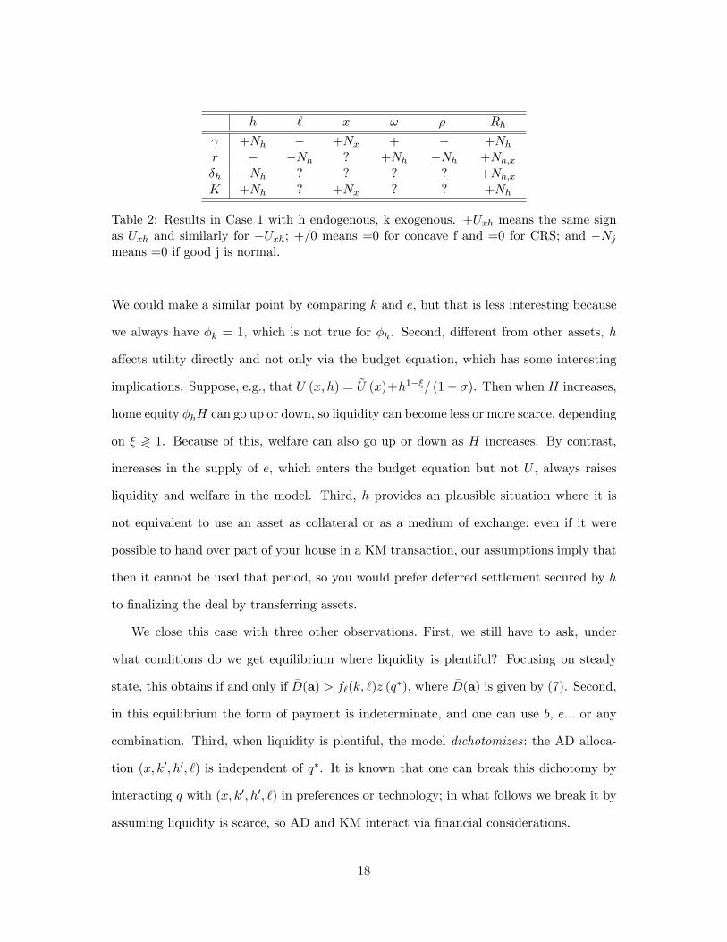
Table 2: Results in Case 1 with h endogenous, k exogenous. +Uxh means the same signas Uxh and similarly for −Uxh; +/0 means =0 for concave f and =0 for CRS; and −Nj

means =0 if good j is normal.

We could make a similar point by comparing k and e, but that is less interesting because

we always have φk = 1, which is not true for φh. Second, different from other assets, h

affects utility directly and not only via the budget equation, which has some interesting

implications. Suppose, e.g., that U (x, h) = U (x)+h1−ξ/ (1− σ). Then when H increases,

home equity φhH can go up or down, so liquidity can become less or more scarce, depending

on ξ ≷ 1. Because of this, welfare can also go up or down as H increases. By contrast,

increases in the supply of e, which enters the budget equation but not U , always raises

liquidity and welfare in the model. Third, h provides an plausible situation where it is

not equivalent to use an asset as collateral or as a medium of exchange: even if it were

possible to hand over part of your house in a KM transaction, our assumptions imply that

then it cannot be used that period, so you would prefer deferred settlement secured by h

to finalizing the deal by transferring assets.

We close this case with three other observations. First, we still have to ask, under

what conditions do we get equilibrium where liquidity is plentiful? Focusing on steady

state, this obtains if and only if D(a) > f`(k, `)z (q∗), where D(a) is given by (7). Second,

in this equilibrium the form of payment is indeterminate, and one can use b, e... or any

combination. Third, when liquidity is plentiful, the model dichotomizes: the AD alloca-

tion (x, k′, h′, `) is independent of q∗. It is known that one can break this dichotomy by

interacting q with (x, k′, h′, `) in preferences or technology; in what follows we break it by

assuming liquidity is scarce, so AD and KM interact via financial considerations.

18

3.2 Illiquid Nonmonetary Equilibrium

Consider next a nonmonetary equilibrium where D (a) is such that buyers cannot get q∗.

The FOC for q implies λq = βσL (q) /ω′ > 0, where

L (q) =u′ (q)− z′ (q)

z′ (q). (24)

Although not strictly necessary, to ease the presentation, assume L′ (q) < 0 ∀q.12 Then

for j 6= m the FOC for dj implies λj = λq∂d/∂dj > 0. Hence, KM buyers borrow to the

limit D(a), and q solves z (q)ω′ = D(a). In terms of asset prices, we have

φb =βω

ω′[1 +D′b(B)σL (q)

](25)

φe =βω

ω′(γ + φ′e

) [1 +D′e(1)σL (q)

](26)

φh = βωUh(x′, h′

)+βω

ω′(1− δh)φ′h

[1 +D′h(h′)σL (q)

](27)

1 =βω

ω′(ρ′ + 1− δk)

[1 +D′k(k

′)σL (q)]. (28)

Compared to (12)-(15), the liquidity premium D′j (aj)σL (q) now appears on the RHS,

because as long as D′j (aj) > 0, having more aj relaxes debt limits.

Suppose h = H is fixed (endogenous h can be handled as above). An illiquid nonmon-

etary equilibrium consists of paths for: (1) (x, k′, h′, `) satisfying

1 = f` (k, `)Ux (x,H) (29)

Ux (x,H) = βUx(x′, H

) [fk(k

′, `′) + 1− δk] [

1 +D′j (k)σL (q)]

(30)

h′ = H (31)

x = γ + f (k, `) + (1− δk) k − k′; (32)

(2) (q, d) satisfying d = D (a) and z (q) = d/ω′; and (3) asset prices as described above.

Compared to the previous case, (30) has 1 + D′j (k)σL (q) multiplying the RHS because

12This condition holds automatically for many standard mechanisms, including Kalai bargaining andWalrasian pricing, but not generalized Nash bargaining. One can prove the same results without assumingL′ (q) < 0 ∀q, as in Wright (2010), but we prefer to avoid these technicalities.

19

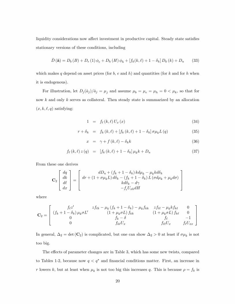
liquidity considerations now affect investment in productive capital. Steady state satisfies

stationary versions of these conditions, including

D (a) = Db (B) +De (1)φe +Dh (H)φh + [fk(k, `) + 1− δk]Dk (k) +Du (33)

which makes q depend on asset prices (for b, e and h) and quantities (for k and for h when

it is endogenous).

For illustration, let Dj(aj)/aj = µj and assume µb = µe = µh = 0 < µk, so that for

now k and only k serves as collateral. Then steady state is summarized by an allocation

(x, k, `, q) satisfying:

1 = f` (k, `)Ux (x) (34)

r + δk = fk (k, `) + [fk (k, `) + 1− δk]σµkL (q) (35)

x = γ + f (k, `)− δkk (36)

f` (k, `) z (q) = [fk (k, `) + 1− δk]µkk +Du (37)

From these one derives

C2

dqdkd`dx

=

dDu + (fk + 1− δk) kdµk − µkkdδk

dr + (1 + σµkL) dδk − (fk + 1− δk)L (σdµk + µkdσ)kdδk − dγ−f

`UxhdH

where

C2 =

f`z′ zf`k − µk (fk + 1− δk)− µkfkk zf`` − µkkfk` 0

(fk + 1− δk)µkσL′ (1 + µkσL) fkk (1 + µkσL) fk` 00 fk − δ f` −10 fk`Ux f``Ux f`Uxx

In general, ∆2 = det (C2) is complicated, but one can show ∆2 > 0 at least if σµk is not

too big.

The effects of parameter changes are in Table 3, which has some new twists, compared

to Tables 1-2, because now q < q∗ and financial conditions matter. First, an increase in

r lowers k, but at least when µk is not too big this increases q. This is because ρ = fk is

20

q k ` x ω ρ

γ − −∗ −∗/0 +∗ +∗/0 −r +∗ − ? − − +H +Uxh +U∗xh +U∗xh +U∗xh −U∗xh +UxhDu + − ? + − +µk ? +∗ −∗ +∗ −∗ −∗σ −∗ + ? + + −

Table 3: Results in Case 2 with k endogenous, h exogenous. Notes: +Uxh means the samesign as Uxh and similarly for −Uxh; +∗ means the result is ambiguous in general but > 0if k is small, and similarly for −∗; and +/0 means = 0 for concave f and =0 for CRS, andsimilarly for −/0..

higher when there is less k, and on net credit constraints can be relaxed. Second, supposing

h and x are complements, if H increases then x and k do, too, so credit constraints ease

with higher H even though µh = 0. The loan-to-value ratio µk has an ambiguous effect

on q, because k rises but ρ falls, and on net debt limits can fall. Similarly, an increases

in σ makes agents put more weight on liquidity, which increases k and hence x, but has

an ambiguous effect on q. Indeed, ∂q/∂σ < 0 is unambiguous when µk is small. One

might call this a paradox of liquidity : individuals can try to relax borrowing constraints

by investing in pledgeable k, but if everyone does so, ρ can fall enough to tighten credit

conditions.

Finally, as in the previous case, we have to ask when this (illiquid nonmonetary) equi-

librium exists. The answer is f` (k, `) z (q∗) > D (a) ≥ f` (k, `) z(qi). The first inequality

says agents cannot borrow enough to get q∗, with D (a) given in (7). The second says

they can borrow enough to get at least what they would get in monetary equilibrium, as

described next.

3.3 Monetary Equilibrium

In monetary equilibrium, the constraints bind, so λq = βσL (q) > 0 and λj = D′j (pj)λq >

0. Again, buyers go to the limit D (a), but now this includes real balances. The equations

for (φb, φe, φh, φk) are the same as above, (25)-(28), and now there is a new the condition

21

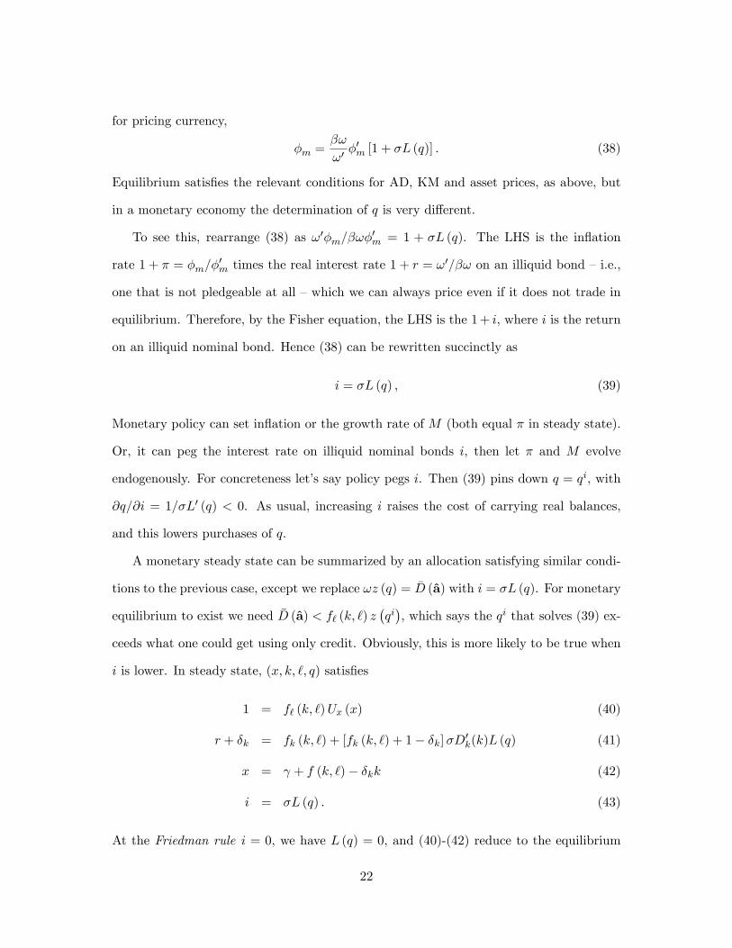
for pricing currency,

φm =βω

ω′φ′m [1 + σL (q)] . (38)

Equilibrium satisfies the relevant conditions for AD, KM and asset prices, as above, but

in a monetary economy the determination of q is very different.

To see this, rearrange (38) as ω′φm/βωφ′m = 1 + σL (q). The LHS is the inflation

rate 1 + π = φm/φ′m times the real interest rate 1 + r = ω′/βω on an illiquid bond —i.e.,

one that is not pledgeable at all —which we can always price even if it does not trade in

equilibrium. Therefore, by the Fisher equation, the LHS is the 1 + i, where i is the return

on an illiquid nominal bond. Hence (38) can be rewritten succinctly as

i = σL (q) , (39)

Monetary policy can set inflation or the growth rate of M (both equal π in steady state).

Or, it can peg the interest rate on illiquid nominal bonds i, then let π and M evolve

endogenously. For concreteness let’s say policy pegs i. Then (39) pins down q = qi, with

∂q/∂i = 1/σL′ (q) < 0. As usual, increasing i raises the cost of carrying real balances,

and this lowers purchases of q.

A monetary steady state can be summarized by an allocation satisfying similar condi-

tions to the previous case, except we replace ωz (q) = D (a) with i = σL (q). For monetary

equilibrium to exist we need D (a) < f` (k, `) z(qi), which says the qi that solves (39) ex-

ceeds what one could get using only credit. Obviously, this is more likely to be true when

i is lower. In steady state, (x, k, `, q) satisfies

1 = f` (k, `)Ux (x) (40)

r + δk = fk (k, `) + [fk (k, `) + 1− δk]σD′k(k)L (q) (41)

x = γ + f (k, `)− δkk (42)

i = σL (q) . (43)

At the Friedman rule i = 0, we have L (q) = 0, and (40)-(42) reduce to the equilibrium

22

conditions for (x, k, `) in Section 3.1. As in many monetary models, i = 0 delivers an

effi cient AD allocation.

In our model, there is still a question of whether i = 0 also delivers KM effi ciency,

q = q∗. The answer depends on the mechanism: it is not hard to verify that i = 0 implies

q = q∗ with Walrasian pricing or Kalai bargaining, but not necessarily with generalized

Nash bargaining unless θ = 1. For Nash with θ < 1, i = 0 is still optimal but it does

not achieve the first best. In this case, it would be desirable to set i < 0, in principle,

but there is no equilibrium with i < 0. This is the New Monetarist version of the New

Keynesian zero lower bound problem. Here, i < 0 would be desirable, if only it were

feasible, because it would correct a problem with Nash bargaining. Still, with any of these

pricing mechanisms i = 0 is the optimal policy in this version of the model, but once we

introduce other distortions, that may no longer be the case. In Section 5, we introduce

capital-income taxation, and find that i > 0 may be optimal.

In any case, setting D (aj) = µjaj and combining (39) and (41), we get

fk (k, `) =r + δk − (1− δk)µki

1 + µki.

While µk affects this condition, it cannot affect q, which is determined by (39). How

can pledgability not affect KM trade? The answer is that in monetary equilibrium i pins

down qi and then qi pins down the debt limit D (a) = f` (k, `) z(qi), not vice-versa.

Heuristically, when the pledgability of a k increases, other forms of liquidity are crowded

out, leaving

D = µbB +(1 + r) γµer − µei

+(1− δh) (Uh/Ux)µhH

r + δh − (1− δh)µhi+ (fk + 1− δk)µkK +Du + φmM

the same. Relatedly, increasing B has no effect on the allocation, as real balances get com-

pletely crowded out. This suggests open market operations, or more generally, quantitative

easing, might not have the impact one expects.

To characterize these and other effects in more detail, one can derive

23

C3

dqdkd`dx

=

Ldσ − di

dr + (1 + µkσL) dδk − (fk + 1− δk)L(σdµk + µkdσ)kdδk − dγ−f`UxhdH

where

C3 =

−σL′ 0 0 0

(fk + 1− δk)µkσL′ (1 + µkσL) fkk (1 + µkσL) fk` 00 fk − δk f` −10 f`kUx f``Ux f`Uxx

and ∆3 = det (C3) = −σL′ (1 + µkσL) Ux |f |+ f` [f`fkk − fk` (fk − δk)]Uxx > 0. The

(extremely sharp) effects of parameters are shown in Table 4, including what is usually

called the Tobin effect,

∆3∂k/∂i = (fk + 1− δk)µkσL′(f2` Uxx + f``Ux

)> 0 if µk > 0.

Intuitively, higher inflation gives households the incentive to substitute k for m in their

portfolios, which is relevant for several of the findings to follow.

q k ` x ω ρ φe

i − + ? + + − +σ + 0 0 0 0 0 0γ 0 − − + 0 0 0µk 0 + ? + + − 0µe 0 0 0 0 0 0 +r 0 − ? − − + 0δk 0 ? ? − − + 0

Table 4: Results in Case 3 with k endogenous, h exogenous.

In particular, since monetary policy affects investment in capital it also affects the

labor market. In general, one cannot sign

∆3∂`/∂i = − (fk + 1− δk)µkσL′ [fk`Ux + (fk − δk) f`Uxx]

and so the Phillips curve can go either way, but if Uxx is small then we know for sure

24

that ∂`/∂i > 0.13 Here movements in ` come along the intensive margin, as changes in

hours worked by the representative individual, but as mentioned above, one can assume

indivisible labor and use lotteries to generate unemployment. The same equations hold

in that model, but now movements in ` come along the extensive margin, as changes in

the number of agents employed. Thus, the model can generate a long-run exploitable

trade-off between inflation and unemployment. Of course, just because it is feasible to

reduce unemployment by increasing inflation, that does not mean it is a good idea. As we

said, i = 0 is optimal here, although it may not be once one introduce other distortions.

In terms of financial parameters, higher µk makes k a better payment instrument, and

so it increases investment, but again q does not change —restricting attention, obviously, to

parameter changes that do not take us out of monetary equilibrium. Similarly, increasing

µe raises the price and lowers the return on e but has no effect on q. In terms of policy’s

impact on returns, increasing i lowers the demand for money and raises the demand for

other assets, which we call a Mundell effect. This helps clarify the nature of Fisher’s

theory that nominal interest rates increase one-for-one with inflation, leaving real returns

the same. One version of this theory, the Fisher equation, says the real return on a illiquid

(nonpledgable) bond is pinned down in steady state by 1+r = 1/β, independent of policy.

But the critical qualification there is that the asset is illiquid.

Fisher’s theory cannot hold for all assets, since m is an asset, with a 0 nominal return,

and so its real return must fall with inflation. How about partially-liquid assets? The real

return on equity is

re =r − µei1 + µei

> 0,

assuming i is suffi ciently low that monetary equilibrium exists. If µe > 0 then ∂re/∂i < 0.

13 If U(x) = x1−η/ (1− η) and f(k, `) = kα`1−α then one can show ∂`/∂i > 0 when η < η, where η > 1.Also, by employment we mean AD labor, since q is not produced. We set it up this way precisely to identifyemployment by `, but alternatively, if q is produced there is an effect going the other way (see Section 5).And we abstract from the effect in Rocheteau et al. (2007) and Dong (2011), where x and q interact inutility, making ∂`/∂i ≷ 0 depend on whether they are substitutes or complelements. Some people seem tothink employment increases with inflation in the data, although our reading is the opposite (see Berentsenet al. (2011) or Figure 5 below). So perhaps it is good the framework is flexible in its prediction for ∂`/∂i.

25

Inflation

Rea

l ret

urns

µ=1µ=00< µ<1

Figure 1: Inflation and asset returns

More generally, for any asset j, ∂rj/∂i ≤ 0 with equality if and only if µj = 0 (i.e.,

if and only if the asset is not pledgeable at all). In Figure 1, the dotted line is the

steady state return on an illiquid asset, 1 + r = 1/β, the solid curve is the real return on

cash, 1 + rm = φ′/φ, and the dashed curve is the real return on an asset with 0 < µj < 1.

Hopefully, this clarifies Fisher’s theory: real returns are independent of inflation for illiquid

but not liquid assets.

4 Extensions

Before getting into the quantitative work, we briefly mention how the framework can be

extended in various directions.14 First, in an stochastic economy liquidity risk is also

a source of variation in asset returns. Intuitively, assets that provide liquidity in states

where it is most needed command a higher premium. Suppose the dividend on the Lucas

tree γ is an i.i.d. random variable with mean γ, and a realization that is known at the

point of KM trade. In monetary equilibrium, the average return on equity is

1 + re =φe + γ

φe=

1 + r

1 + µei− µecov [L (q) , γ/φe]

1 + µei.

The first term on the RHS is the same as before; the second is an adjustment for risk,

making re lower if the dividend γ is big in states when λq is high.

14 It is possible to skip this Section without loss of continuity.

26

Lagos (2010, 2011) assumes b is riskless while e has a random dividend. Then the

excess return on equity has two parts, one coming from the liquidity differential and one

from risk:

re − rb =(1 + r) (µb − µe) i(1 + µei) (1 + µbi)

− µecov [L (q) , γ/φe]

1 + µei.

Notice this premium depends on the policy variable i. Although this can be explored in

more detail, we focus below on the pure liquidity premium. But to be clear, there are two

parts to Lagos’approach. One is that differences in µj help explain re − rb. The other is

to notice that even if µe = µb liquidity affects how one interprets the data. Heuristically,

suppose re = 6% and rb = 1%. A factor of 6 looks like a lot to explain based on risk. But

suppose the liquidity value of both assets is worth 4%. Then the “corrected”return on e

is 10% and on b is 5%, only a factor of 2.

Next, we mention that it is easy to allow match-specific pledgability limits: the loan-

to-value ratio µj for asset j can depend on who one trades with in the KM market. It

is worth pursuing this, in general, but here we only use the idea to demonstrate one way

of making pledgability endogenous, following Lester et al. (2012). Suppose there are two

assets, e and m. Every seller takes m at face value, while there are two technologies for

enforcing debt secured by e. The first is free, and allows creditors to seize µ1e in the

event of a default. The second has a fixed cost κ, and enables sellers to seize µ2e, with

µ2 > µ1.15 Let us assume κs has to be paid each period in the AD market, although

it is also interesting to consider once-and-for-all investments. The cost is specific to the

individual: agent s ∈ [0, 1] must invest κs ∈ [κ, κ] to access the superior technology.

Labeling agents so that κs is increasing in s, let H(κ) be the corresponding CDF

with support [κ, κ]. Let χ be the endogenous fraction of agents that invest in the better

technology. Conditional on being a KM seller, one’s only relevant characteristic is whether

one has made the investment. Conditional on being a buyer, χ is the fraction of meetings

15One can imagine that sellers do not always know the quality of equity, say, and seizing a lemon orcounterfeit asset entails no cost for a defaulter. A seller that invests in the requisite information to discernasset quality can accept more assets as collateral. See Lester et al. (2012) for more discussion.

27

where µe = µ2. The benefit for a seller from having the better technology, depending on

the measure of others who have it, is

Ω = Ω(χ) ≡ z(q2)− c(q2)− z(q1) + c(q1),

where q1 and q2 are KM output in the two types of meetings, which depend on χ.

The investment decision of agent s is obvious: invest if Ω (χ) exceeds κs. Defining

T (χ) = H [maxs : κs ≤ βσΩ(χ)], an equilibrium with endogenous pledgability is a fixed

point χ = T (χ). While T (χ) is not necessarily continuous, Lester et al. (2012) show

assuming Kalai bargaining that it is increasing. Heuristically, if more sellers have the

µ2 technology, it is easier to use e as collateral, which increases the demand for e. This

increases the price φe and makes agents more keen on being able to trade using e as

collateral, so χ goes up. Hence, by Tarski’s fixed point theorem an equilibrium exists.

There can easily be multiple equilibria, and it is possible that no one invests in the superior

technology χ = 0, where everyone does χ = 1, and where a fraction does χ ∈ (0, 1). Also,

pledgability is not invariant to changes in policy in this economy: the ability to get a loan

secured by e changes when i changes.

One can also make pledgability endogenous with a simple moral-hazard model. Again

consider two assets, e and m, and suppose the former requires maintenance to yield the

full dividend γ. Agents with e units of equity choose a maintenance level n ∈ [0, 1], after

trading, at a utility cost εne. Given n the dividend per unit of equity is nγe. In principle,

a debtor can choose to not maintain an asset that has been pledged to a creditor, renege

on his obligation, and forfeit e. One can show (details available on request) the inability

of debtors to commit to n leads to an endogenous pledgability limit De(e) = µee with

µ = 1 − εω′/ (γ + φe). That arises because he will maintain the asset to keep the return

to his share (after forfeiture) high. Also, when all agents face the same maintenance cost

ε, then it is equivalent to use the asset as a medium of exchange or as collateral. But this

is no longer true when ε differs across agents.

28

Suppose there are two types, with costs ε1 and ε2 > ε1, and the fraction of type-1

agents is common knowledge. We consider two cases: ex-ante heterogeneity, where type

is perfectly observed in the KM market; and ex post heterogeneity, where type is realized

after KM trade and only privately observed. In the first case, collateralized borrowing can

be strictly preferred in some meetings, and transfers in others. The intuition is simple:

if one agent is known to be better at maintaining the value of e, then he should hold

it. But if differences emerge after KM trade, and again are privately observed, immediate

transfers may better facilitate transactions. Private information limits the extent to which

ex post liquidity can be pledged. Thus, assets characterized by observable differences in

the ability to maintain value are more likely to used as collateral. We only touch on this

idea briefly, but think there is potential for future work. See Holmstrom and Tirole (2011)

for more discussion of these kinds of issues. Our point is that it is possible to endogenize

pledgability, in various ways, and it is surely interesting, but for the rest of this paper the

debt limits are exogenous.

5 Quantitative Analysis

We now ask what the theory has to say quantitatively, focusing on the effects of monetary

policy and financial innovation. We emphasize that this is not a business cycle analysis;

the interest is on longer-run phenomena. In terms of the model, this means looking at dif-

ferences across steady states, or deterministic transitions between steady states, although

one can simulate the model with shocks to monetary, financial and other variables. In

terms of the data, this means we are mainly interested in observations after filtering to

remove higher-frequency effects. This is partly because we want the empirical analysis to

correspond to the analytic results in Section 3, and partly because we think longer-run

changes in monetary and financial variables are more interesting. Also, to hopefully avoid

confusion, we are not claiming that inflation or financial innovation were the only driving

forces in the data. The exercises are in the nature of controlled experiments, or numer-

29

ical partial derivatives, when we ask, counterfactually, what would the model predict if

something were the sole driving force? While this is not the only possible approach, it has

much precedent, including the practice in macro following Kydland and Prescott (1982)

of asking what a model would predict if technology shocks were the sole impulse.

By way of preview, here are some findings:

• liquidity effects can generate a large return premium for assets that are less pledge-

able;

• the model can account quite well for the effects of changes in inflation on standard

macro aggregates in the data;

• the calibrated parameters imply that reducing inflation to the Friedman rule leads

to a decrease in welfare;

• the optimal inflation rate is close to the average rate observed in the data, although

this is somewhat sensitive to changes in specification;

• financial innovation can generate significant movements in asset prices and economic

activity, including expansions and recessions fueled by housing markets.

Before proceeding, we make three minor changes to the model. First, we set Du =

0, and ignore Lucas trees, leaving four assets to facilitate intertemporal exchange: a =

(b, h, k,m). Second, we add proportional taxes on labor income and asset income (the

returns to b and k), denoted τ ` and τa, and assume pledgability limits are post-tax:

db ≤ [1− (1− φb) τa]µbb and dk ≤ [1 + (ρ− δk) (1− τa)]µkk. While taxes would have

been a distraction for the analytic results, they are critical for calibration. Third, the

probability that a household needs a KM loan each period is now σ ∈ [0, 1]. When

households were interpreted as trading bilaterally in the KM market, previously, we have

σ ∈ [0, 1/2] since not more than a fraction σ = 1/2 can be buyers if each one needs a seller.

However, to match some observations, it it helps to allow σ > 1/2. This is no problem for

30

the theory, as one can simply assume some sellers produce for multiple buyers in the KM

market, without changing any of the relevant equations discussed above.

Also, we address a measurement issue. With the KM sector modeled as a pure-

exchange market, total output in the model economy is well defined according to standard

accounting practice —AD output plus KM output all measured in numeraire —and total

employment comes only from AD hours. But there are alternative approaches. What if

not all KM activity is recorded in the data? At least part of this activity involves cash

transactions, some of which may not show up in the offi cial accounts.16 Moreover, in-

stead of making KM a pure exchange market, one can assume that q is produced and add

KM labor to total employment. Usually we stick to the benchmark interpretation, where

q is counted in GDP while only ` is counted as employment, but we also discuss some

implications of changing this interpretation.

5.1 Calibration

Functional forms are standard. The AD utility and production functions are U (x, h, `) =

log x + ψ log h − ζ` and f(k, l) = kαl1−α. The KM utility and cost functions are u(q) =

υq1−η/ (1− η) and c(q) = q. The housing cost function is g(I) = I1+ξ/ (1 + ξ), where

I = H ′ − (1− δh)H is net residential investment. As discussed above, the KM terms of

trade are determined by Kalai bargaining, z(q) = (1− θ)u(q) + θc(q), although Walrasian

pricing emegres as a special case when θ = 1. As in much of the literature, α in the

AD production function is set to 0.33 to match labor’s and capital’s shares in the income

accounts. We let the time period be a year, and set β = 0.95 so the annual real interest rate

on a illiquid bond is 5.26%. However, interest rates on liquid assets can be considerably

lower, and 5.26% should be interpreted as the return one would require if an asset could

not be used as collateral at all. Estimates of marginal tax rates, especially τa, vary widely,

but we use τa = 0.4 and τ ` = 0.3, in the range of previous studies.

16 In Wallace (2010) and Aruoba (2010), the analog of our KM market is interpretted as the undergroundeconomy. That would be going to far for our purposes of this paper, but we wanted to mention it.

31

The remaining parameters are calibrated to match some observations for the U.S. over

the period 1954-2000 (unless otherwise noted). There are two reasons for stopping at 2000.

First, we do not claim to have a great theory of the great contraction, although we believe

models that take financial considerations seriously may be on the right track. Second, even

before the crisis, developments in financial and housing markets make the 2000’s “special.”

As Holmstrom and Tirole (2011) say, “In the runup to the subprime crisis, securitization

of mortgages played a major role ... by making nontradable mortgages tradable, [and

this] led to a dramatic growth in the US volume of mortgages, home equity loans, and

mortgage-backed securities in 2000 to 2008.”As Ferguson (2008) or Reinhart and Rogoff

(2009) put it, this allowed consumers to start treating their houses as “ATM machines”

(see also Mian and Sufi (2011)). To be clear, the recent period is not a “problem”for the

theory, which in fact puts front and center issues relating to credit and pledgability. But

our strategy is to calibrate to more “normal”times, then see what the model says about

events since the turn of the millennium after adjusting the financial parameters.

The Appendix contains details of the data sources, although housing is the only series

that merits discussion. For this, the value of structures plus land is taken from Davis

and Heathcote (2007), which has the disadvantage of starting only in 1975, but has the

advantage of reliability, mainly because it tries to measure land values accurately. To

this we add consumer durables since many of these (e.g., home appliances) are part of

household capital. To be consistent, the value of housing services is removed from the GDP

data, and durable consumption is added to residential investment. Annual depreciation

rates are set to δh = δk = 0.10 to approximately match investment rates in h and k.

These numbers are slightly higher than those seen in some other studies, at least in part

due to the way we adjust our housing and output measures. Inflation averages 3.7% in

our sample. Given this, and an average pre-tax real return on 3-month T-bills of 1.8%,

we can pin downs µb = 0.45 from the optimality condition for b, which with taxes is

1 + rb = [1 + r − (1 + µbi) τa] /(1 + µbi) (1− τa).

32

This leaves 10 parameters, (η, υ, σ, θ, ψ, ξ, µk, µh, ζ), which are calibrated as follows.

The KM parameters — the curvature and level of utility η and υ, plus the fraction of

agents needing a loan σ —are set to fit: (1) the empirical relationship between inflation

and M/PY (money demand or inverse velocity), defined using sweep-adjusted M1 data,

consistent with the idea that in this model m can well represent money in the bank; and

(2) the empirical relationship between inflation and real output. While (1) is standard

procedure, (2) is less so and deserves discussion, but we defer that until we see some

results. The remaining 7 parameters are set to match the following targets:17

1. Housing capital over GDP: 1.92.

2. Housing investment over GDP: 0.15.

3. Market capital over GDP: 1.25.

4. T-bills outstanding over GDP: 0.10.

5. Hours worked over discretionary time: 0.33.

6. The KM markup, price z(q)/q over marginal cost c′ (q): 1.30.

7. Home equity loans over housing wealth: 0.03.

Table 5 summarizes the baseline calibration, as well as an alternative calibration dis-

cussed below. Although the parameters are set jointly to match the targets, heuristically

one can think of subsets of parameters being identified by subsets of the targets, as de-

scribed in the Table. Already from these numbers one can ask how the model does in

17Thess targets are mostly standard, although a couple of comments may be warranted. As in Aruobaet al. (2011), the markup comes from the Annual Retail Trade Survey. In these data, at the low end,Warehouse Clubs, Superstores, Automotive Dealers and Gas Stations have markups between 1.17 and1.21; at the high end, Specialty Foods, Clothing, Footware, and Furniture have markups between 1.42and 1.44; so we target 1.3. Also, for µh, we need to adjust for two factors. First, around 30% of homecapital is used to collateralize mortgages, and is therefore not available to secure household consumptionloans. Thus, home equity is given by 0.7 (1− δh)φhh = 0.63φhh. Second, in the model, only a fractionσ of households need loans in any period. So home equity loans over housing wealth is 0.63σµh. Given atarget for this ratio and a choice for σ, we pin down µh.

33

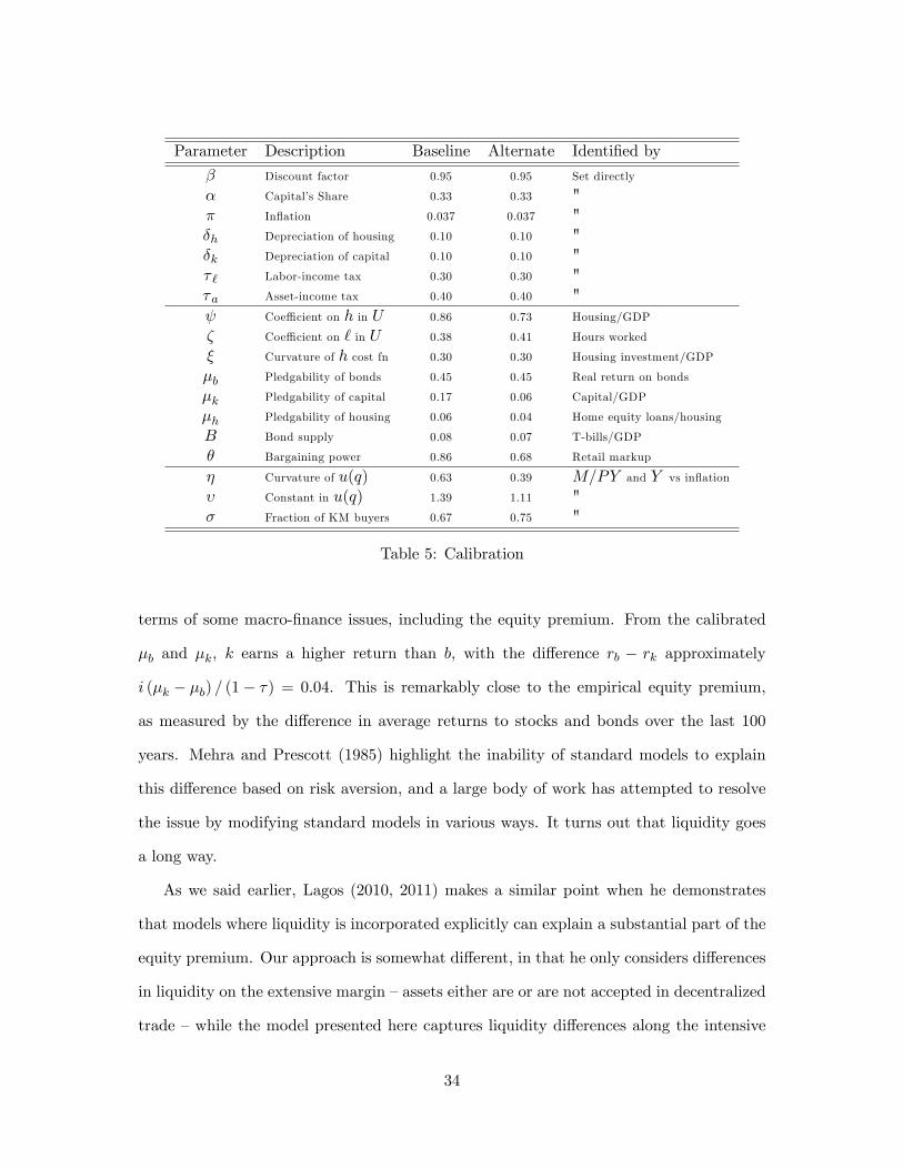
Parameter Description Baseline Alternate Identified by

β Discount factor 0.95 0.95 Set directly

α Capital’s Share 0.33 0.33 "π Inflation 0.037 0.037 "δh Depreciation of housing 0.10 0.10 "δk Depreciation of capital 0.10 0.10 "τ ` Labor-income tax 0.30 0.30 "τa Asset-income tax 0.40 0.40 "ψ Coeffi cient on h in U 0.86 0.73 Housing/GDP

ζ Coeffi cient on ` in U 0.38 0.41 Hours worked

ξ Curvature of h cost fn 0.30 0.30 Housing investment/GDP

µb Pledgability of bonds 0.45 0.45 Real return on bonds

µk Pledgability of capital 0.17 0.06 Capital/GDP

µh Pledgability of housing 0.06 0.04 Home equity loans/housing

B Bond supply 0.08 0.07 T-bills/GDP

θ Bargaining power 0.86 0.68 Retail markup

η Curvature of u(q) 0.63 0.39 M/PY and Y vs inflation

υ Constant in u(q) 1.39 1.11 "σ Fraction of KM buyers 0.67 0.75 "

Table 5: Calibration

terms of some macro-finance issues, including the equity premium. From the calibrated

µb and µk, k earns a higher return than b, with the difference rb − rk approximately

i (µk − µb) / (1− τ) = 0.04. This is remarkably close to the empirical equity premium,

as measured by the difference in average returns to stocks and bonds over the last 100

years. Mehra and Prescott (1985) highlight the inability of standard models to explain

this difference based on risk aversion, and a large body of work has attempted to resolve

the issue by modifying standard models in various ways. It turns out that liquidity goes

a long way.

As we said earlier, Lagos (2010, 2011) makes a similar point when he demonstrates

that models where liquidity is incorporated explicitly can explain a substantial part of the

equity premium. Our approach is somewhat different, in that he only considers differences

in liquidity on the extensive margin —assets either are or are not accepted in decentralized

trade —while the model presented here captures liquidity differences along the intensive

34

margin —assets are accepted only up to certain limits. The point is not that these two

approaches are so very different; rather, we want to emphasize how models of this general

class have considerable potential for studying macro-finance issues in various ways. The

message is that these models are potentially useful for understanding many observations

that are diffi cult to capture with models that ignore liquidity considerations.

5.2 Main Results

To begin, Figure 2 shows steady state values for the standard macro aggregates as a

function of inflation π, from a high of 10% to a low of −0.05, the value associated with the

zero lower bound on i, or the Friedman rule. Inflation is bad for KM consumption q, as we

knew from the analytic results, but now we see the effect is sizable: reducing π from 10%

to the Friedman rule increases q from around 1.1 to 1.7, and even reducing π from 10% to

0 increases q to almost 1.5. Offsetting this is the higher AD consumption x, which results

mainly from k increasing due to the Tobin effect. The increase in k also generates an

increase in employment, although the scale on the vertical axis indicates that this effect is

not very big (we return to this below). Although this is not true for all parameter values,

for the calibrated values, total output increases with π, as the increase in AD production

more than offsets the fall in KM trade.

The value of the housing stock φhh also increases with inflation, consistent with the

facts documented in various data sources for the U.S. and other countries by Aruoba

et al. (2012), but the explanation is totally different. The suggestion there is that agents

substitute out of market and into household production as π increases, leading to higher

demand for inputs into household production, including houses. Here the demand for h

increases with π as agents try to substitute other pledgeable assets for cash, similar to the

effect on k. An advantage of our explanation is that it has h and k both rising with π in

the model, as in the data (see below); the other story tends to have them move it opposite

directions. Something similar applies to bonds, which we emphasize because T-bills are

35

­0.05 0 0.05 0.10.75

0.76

0.77

0.78

0.79

0.8

0.81

0.82Output, y( π)

­0.05 0 0.05 0.10.23

0.24

0.25

0.26

0.27

0.28

0.29AD Consumption, x( π)

­0.05 0 0.05 0.11.1

1.2

1.3

1.4

1.5

1.6

1.7

1.8KM Consumption, q( π)

­0.05 0 0.05 0.10.315

0.32

0.325

0.33

0.335

0.34

0.345Labor, l( π)

­0.05 0 0.05 0.10.7

0.8

0.9

1

1.1

1.2

1.3

1.4Capital stock, k( π)

­0.05 0 0.05 0.11.35

1.4

1.45

1.5

1.55

1.6

1.65

1.7

Housing stock, φh H(π)

Figure 2: Inflation and aggregate variables (baseline calibration).

the subject of a recent empirical study by Krishnamurthy and Vissing-Jorgensen (2012).

Figure 3 shows how π reduces the returns to b, k and h, which we knew from the analytic

results, but here we quantify the effects, with the fall in rb larger than in rh and rk, since

the calibration implies b is more pledgeable. The lower left panel of Figure 3 shows the

fall in real balances with π, while the next panel shows the increase in liquidity from other

assets, D− φmM . On net, total liquidity falls —or credit tightens —with π since q falls.18

The last panel of Figure 3 shows the cost of inflation, computed as the change in AD

consumption that gives the same increase in utility as switching to the Friedman rule,

not across steady states, but taking into account the transition as k and h adjust. In the

calibrated model this cost is negative —i.e., switching to the Friedman rule is equivalent

to a reduction in x. In terms of magnitude, going from the average π in the sample to

18Part of the fall in q is due to an increase in the wage ω, since z (q)ω/ζ = D means that at higherwages KM buyers get less for their money.

36

­0.05 0 0.05 0.10.95

1

1.05

1.1

Return on bonds, r b(π)

­0.05 0 0.05 0.10.95

1

1.05

1.1

Return on capital, r k(π)

­0.05 0 0.05 0.10.95

1

1.05

1.1

Return on housing, r h(π)

­0.05 0 0.05 0.10.1

0.15

0.2

0.25

0.3

0.35

Real balances, φm M( π)

­0.05 0 0.05 0.10.22

0.24

0.26

0.28

0.3

0.32Liquidity, D( π)

­0.05 0 0.05 0.1­0.02

­0.015

­0.01

­0.005

0

Welfare gains, ∆x(π)

Figure 3: Inflation and aggregate variables (baseline calibration).

the Friedman rule is like reducing x about 1.5%. This is due to the tax τa, which tends

to make k too low. Inflation is beneficial because the Tobin effect partially offsets the

tax effect on k, more than compensating for the effect on q. If π did not affect k then

going from π = 0.1 to the Friedman rule would be like an increase in x of nearly 5%,

purely due to the impact on q. This is much higher than what one finds in reduced-form

models like Lucas Jr (2000), but similar to Lagos and Wright (2005). Even with this big

impact on q, the beneficial impact on k, absent in Lucas Jr (2000) or Lagos and Wright

(2005), is the dominating effect. Without taxes the Friedman rule is optimal; with taxes,

the calibration implies the optimal inflation rate is 3.5%, which is surprisingly close to the

average inflation rate in the data.

While these results seem interesting, especially the welfare effects, one might wonder if

the model does well enough at capturing the data for us to take them seriously. The answer

37

0 0.05 0.10.68

0.7

0.72

0.74

0.76

0.78Consumption­Output, C( π)/Y

0 0.05 0.11

1.2

1.4

1.6

1.8Capital­Output, k( π)/Y

0 0.05 0.11.7

1.8

1.9

2

2.1

2.2

Housing­Output, φh H(π)/Y

0 0.05 0.10.1

0.15

0.2

0.25

0.3

0.35

Inverse velocity, φm M( π)/Y

0 0.05 0.10.3

0.32

0.34

0.36

0.38

0.4Labor, l( π)

0 0.05 0.10.95

1

1.05

1.1

Return on bonds, rb(π)

Figure 4: Inflation and ratios (baseline calibration): ∗ = data; = HP trends.

38

seems to be yes. Figure 4 overlays some model relationships with the facts, normalizing

nonstationary variables by GDP (e.g., reporting k/y rather than k). The stars indicate raw

data, and the circles indicate HP trends with filtering parameter 100. These pictures reveal

that changes in inflation over the period account for a significant fraction of movements in

the data, especially the lower-frequency components captured by the filtered series. The

only relationship shown in Figure 4 that was fit in the calibration routine isM/PY versus

inflation, yet the model is in line with data in terms of c/y, k/y, h/y and rb.19

The one dimension along which the model does less well is the labor market: it gen-

erates a fairly flat but slightly upward-sloping relationship, somewhat at odds with the

data. There are two points to make about this. First, one can argue that the scatter plot

of π versus ` is basically a “cloud,” as Christiano and Eichenbaum (1992) argue for the

relationship between productivity and `, and hence, as they conclude, one is not going to

match the data with any one forcing variable. Second, as we said above, one can interpret

employment differently in the model by having production in the KM market. Figure 5

compares the model-implied Phillips curve to the data under the two interpretations of

labor. The left panel is reproduced from the baseline results, which only count AD labor.

The right panel adds ` and q, assuming the KM technology produces output one-for-one

with hours, and rescaling the sum so that the model is still consistent with the calibration

target 0.33. Under this interpretation, the model lines up reasonably well with the facts.

While we do not want to oversell any match between model and data, we feel obliged to

defend its relevance against the obvious critique that it is generated assuming no changes

in other driving forces, including taxes, technology shocks etc. As explained above, it

standard in macro to ask, counterfactually, what might have happened in the economy if

the only driving process were changes in some variable z. Here z is given by medium-run

changes in inflation, and the answer is that the main variables of interest would have

19 In fact, in this baseline calibration we also targeted the inflation-output relationship, although this haslittle to do with Figure 4. As shows below, even if we do not try to match that relationship, the results in4 look very much the same.

39

0 0.02 0.04 0.06 0.08 0.1

0.3

0.32

0.34

0.36

0.38

0.4Model (AD labor) versus Data

0 0.02 0.04 0.06 0.08 0.1

0.3

0.32

0.34

0.36

0.38

0.4Model (AD+KM labor) versus Data

Figure 5: Phillips curves.

looked a lot like what was observed in the data. This should shift one’s prior toward

thinking that maybe inflation is interesting and that the model is reasonable. One still

ought to think about robustness, however, particularly with respect to the choice of the

targets generating the parameter values.

Much of our calibration strategy follows well-worn paths, except perhaps matching the

relationship between filtered output and inflation. One can try to set the KM parameters

(η, υ, σ) to match only the empirical money demand relationship, although identification is

fairly weak —i.e., there are different combinations of these parameters that fit the M/PY

versus π data about as well. Table 5 shows the alternative calibration where only M/PY

versus π data are used to set (η, υ, σ). The main change is in the value for µk. Figures 6-7

show the results for this calibration, while Figure 8 overlays the relevant data. Comparing

these to Figures 2-4, for most variables the results are very similar, and the predictions for

the ratios k/y, c/y etc. are still in line with the data. This implies that many predictions

are robust along this dimensions, but there are two exceptions.

First, the baseline model predicts that output increases with π, while the alterna-

tive predicts that it falls. This is driven by the difference in the pledgability of capital.

Specifically, the baseline calibration selects values for (η, σ, υ) that require a higher µk to

match the target capital-ouput ratio, and this makes the Tobin effect stronger. Second,

40

­0.05 0 0.05 0.10.62

0.64

0.66

0.68

0.7

0.72

0.74Output, y( π)

­0.05 0 0.05 0.10.255

0.26

0.265

0.27

0.275AD Consumption, x( π)

­0.05 0 0.05 0.1

0.7

0.8

0.9

1

1.1

1.2

1.3

1.4KM Consumption, q( π)

­0.05 0 0.05 0.10.324

0.326

0.328

0.33

0.332

0.334

0.336

0.338Labor, l( π)

­0.05 0 0.05 0.10.75

0.8

0.85

0.9

0.95Capital stock, k( π)

­0.05 0 0.05 0.11.22

1.24

1.26

1.28

1.3

1.32

1.34

1.36

Housing stock, φh H(π)

Figure 6: Inflation and aggregate variables (alternative calibration).

there is a big difference in the implications for welfare. Welfare rises with π over a broad

range in the baseline model, since ameliorating the tax-related investment distortion more

than compensates for the decline in KM activity. This is not true for the alternative

calibration, where the KM effect dominates, and there are substantial welfare losses from

positive inflation. In particular, reducing π from 10% to the Friedman rule is worth al-

most 5% of x, and the optimal inflation rate is now negative, although above the Friedman

rule. So, while many of the positive implications of the theory are robust, the normative

implications are sensitive to the parameterization.20

In terms of other robustness issues, we recalibrated the model after setting θ = 1,

which can be interpreted as Walrasian pricing. The results (not shown) are similar to the

20We discuss this more, in the context of the empirical literature on the effects of inflation, in theConclusion.

41

­0.05 0 0.05 0.10.95

1

1.05

1.1

Return on bonds, rb(π)

­0.05 0 0.05 0.10.95

1

1.05

1.1

Return on capital, rk(π)

­0.05 0 0.05 0.10.95

1

1.05

1.1

Return on housing, rh(π)

­0.05 0 0.05 0.10.05

0.1

0.15

0.2

0.25

0.3

Real balances, φm

M( π)

­0.05 0 0.05 0.10.125

0.13

0.135

0.14

0.145Liquidity, D( π)

­0.05 0 0.05 0.1­0.01

0

0.01

0.02

0.03

0.04

0.05

Welfare gains, ∆x(π)

Figure 7: Inflation and aggregate variables (alternative calibration).

benchmark, although q is higher, the loss from going to the Friedman rule is slightly lower,

and there are minor differences in the effects of π on k and h. Where θ = 1 misses, of

course, it that it gives a KM markup of 0 rather than 0.3. We also checked robustness by

shutting down taxes. The results (not shown) are very different from the benchmark, which

is no surprise, since it is well known that taxes have big effects on capital accumulation

(e.g., McGrattan et al. (1997)). Consider the cost of inflation. With τa = τ ` = 0, going

from π = 0.1 to the Friedman rule, which is now optimal, is worth nearly 18% of x, with

about half coming from KM and half from AD. Even going from π = 0.04 to the Friedman

rule is worth nearly 5% of x. We do not think these numbers are too meaningful, however,

since taxation is a fact of life, making τa = τ ` = 0 not a compelling calibration. What

we take away from this is that π has a big impact on consumption, but this is offset by

partially correcting tax distortions on investment.

42

0 0.05 0.10.68

0.7

0.72

0.74

0.76

0.78Consumption­Output, C( π)/Y

0 0.05 0.11

1.2

1.4

1.6

1.8Capital­Output, k( π)/Y

0 0.05 0.11.7

1.8

1.9

2

2.1

2.2

Housing­Output, φh H(π)/Y

0 0.05 0.10.1

0.15

0.2

0.25

0.3

0.35

Inverse velocity, φm M( π)/Y

0 0.05 0.10.3

0.32

0.34

0.36

0.38

0.4Labor, l( π)

0 0.05 0.10.95

1

1.05

1.1

Return on bonds, rb(π)

Figure 8: Inflation and ratios (alternative calibration): ∗ = data; = HP trends.

43

0 0.2 0.40.75

0.755

0.76

0.765

0.77

0.775

0.78

0.785

Output, y( µh)

0 0.2 0.40.235

0.24

0.245

0.25

0.255

0.26

AD Consumption, x( µh)

0 0.2 0.41.3

1.4

1.5

1.6

1.7

1.8

KM Consumption, q( µh)

0 0.2 0.40.315

0.32

0.325

0.33

0.335

0.34

0.345

Labor, l( µh)

0 0.2 0.40.7

0.75

0.8

0.85

0.9

0.95

1

Capital stock, k( µh)

0 0.2 0.41.35

1.4

1.45

1.5

1.55

1.6

1.65

1.7

Housing stock, φh H(µh)

Figure 9: Housing pledgability and aggregate variables.

One can also use the model to quantify the effects of financial innovation, interpreted

as changes in the pledgability parameters. Figure 9 shows the effect of raising µh. When

µh is small, an increase leads to a housing boom, combined with higher output, investment

and employment; as the innovation continues, however, it ultimately leads to a bust, with

declines in output, investment, employment and the housing market. The reason is that as

liquidity becomes more abundant, its marginal value decreases, reducing liquidity premia

and asset prices. In particular, once liquidity is suffi ciently abundant that buyers can get

at least qi on credit, money is no longer valued. The kinks in the graphs indicate points

where we switch across the different regimes (types of equilibria) described in Section 3,

but recall that one does not have to take the nonmonetary regime literally, since some

agents in the real world may always use cash.

He et al. (2012) use a related but simpler model to evaluate the possibility that financial

44

0 0.2 0.4 0.60.65

0.7

0.75

0.8

0.85

0.9

Output, y( µk)

0 0.2 0.4 0.60.23

0.24

0.25

0.26

0.27

0.28

0.29

AD Consumption, x( µk)

0 0.2 0.4 0.61.3

1.4

1.5

1.6

1.7

1.8

KM Consumption, q( µk)

0 0.2 0.4 0.60.315

0.32

0.325

0.33

0.335

0.34

0.345

Labor, l( µk)

0 0.2 0.4 0.60.7

0.8

0.9

1

1.1

1.2

1.3

1.4

Capital stock, k( µk)

0 0.2 0.4 0.61.35

1.4

1.45

1.5

1.55

1.6

1.65

1.7

Housing stock, φh H(µk)

Figure 10: Capital pledgability and aggregate variables.

innovation spurred the U.S. experience since 2000, along with alternatives, like bubbles as

self-fulfilling prophecies. The findings are similar: while a housing-fueled expansion and

contraction can be explained qualitatively by developments in home-equity loan markets,

it is diffi cult to match the facts quantitatively. The ratio of the value of the housing stock

(the last panel of Figure 9) to GDP (the first panel) peaks at just over 2, while in the

data it reached approximately 2.76 at the height of the boom. Hence, while financial

developments may have been significant, there is room for other forces in accounting for

the facts. For comparison, Figure 10 repeats the analysis for an increase in µk. As with µh,

the impact on output, employment, capital and housing is first positive and then negative,

for the same reason. What is not reported in these figures is that increases in pledgability

typically improve welfare. The general rule is that improvements in credit conditions can

be good, even if it looks bad for some macro aggregates.

45

6 Conclusion

We began by thinking about the role of assets in facilitating intertemporal exchange with

limited commitment, and other frictions, as stressed by Kocherlakota (1998) and Wallace

(2010). A key ingredient in the logic was the asynchronization of receipts and expenditure:

sometimes —in the model, in the KMmarket —agents have demands but no current income,

and therefore they need loans. Credit was modeled after Kiyotaki and Moore (1997, 2005),

except we concentrate on consumers rather than producers, in the spirit of Kehoe and

Levine (1993, 2001), Alvarez and Jermann (2000) and incomplete-market models generally

going back at least to Bewley (1977). Debt limits are endogenized by a limited ability

to punish defaulters by seizing assets, guided by work on the microfoundations of money

going back to Kiyotaki and Wright (1989, 1993), updated using recent advances in the

field. A difference from most monetary economics is that agents do not use some asset as

a medium of exchange; rather, they have a portfolio, each element of which can be used

to a greater or lesser extent to collateralize loans. Motivated by Holmstrom and Tirole

(2011), the focus is on pledgability.

Although it nests standard growth and asset-pricing theories as special cases, the

framework is still very tractable. To some readers some ingredients might be unfamiliar,

like the use of abstract pricing mechanisms in the credit market, but these are standard

tools in modern monetary economics, and they make a difference for quantitative work as

well as theory. In terms of substantive questions, we used the model to study several issues

in macro and financial economics. We analyzed how inflation affects the returns to assets

as a function of their pledgability, and how it affects output and employment. We showed

there is crowding out of liquidity in monetary economies, e.g., higher inflation reduces

real balances, but as this impinges on the demand for alternative assets, total liquidity

changes by less than real balances. Relatedly, increases in one asset’s pledgability crowds

out other forms of liquidity. Although one can derive many of these results analytically,

46

we also presented a quantitative analysis, calibrating the model using standard practice

and using it to experiment with monetary policy and financial innovation.

The quantitative results imply that over a relevant range inflation increases output,

employment, investment and some but not all consumption, due to a Mundell-Tobin effect.

While the nominal returns on illiquid assets go up one-for-one with inflation, nominal

returns on liquid assets go up significantly less. This is especially true for bonds, which

are very liquid according to the calibration, and hence earn a lower return than capital,

consistent with the observed equity premium. The price and quantity of housing increase

with inflation, consistent with recent explorations of the data, although our explanation

is different. The benchmark model also implies welfare is increasing in inflation over a

relevant range, due to the Mundell-Tobin effect combined with investment being too low

due to taxes on asset income. For the baseline calibration, the optimal inflation rate was

just about the mean in the data, but this is somewhat sensitive to the parameterization.

In an alternative calibration, the predictions for most of the variables are similar, except

inflation decreases output and the optimal inflation rate is negative.

It is therefore crucial to know whether inflation increases output in the data. There is

a big literature on this, but we can discuss it only briefly here. Bullard and Keating (1995)

find that permanent changes in inflation do not increase in real output for most countries,

but do for some (low-inflation) countries. Ahmed and Rogers (2000) conclude from a

century of U.S. data that “the long-run effects of inflation on consumption, investment,

and output are positive ... [and] ratios like the consumption and investment rates are not

independent of inflation, which we interpret in terms of the Fisher effect.”Therefore, they

say “models generating long-term negative effects of inflation on output and consumption

seem to be at odds with data.”On the other hand, for OECD economies Madsen (2003)

finds investment is negatively related to inflation. In terms of returns, King and Watson

(1997) find nominal interest rates do not adjust one-for-one with permanent inflation, for

47

many plausible identification schemes.21

After surveying much literature, Bullard (1999) concludes: “While the overall evidence

on these questions is mixed, considering only lower inflation countries leads to the conclu-

sion that permanently higher money growth or inflation is associated with permanently

higher output and permanently lower real interest rates.”He also says “this result is in-

consistent with many —almost all? —current quantitative business cycle models, which

generally predict that permanently higher inflation permanently lowers consumption and

output. There is little support for such a prediction in the studies surveyed here. This is

an important empirical puzzle that stands as a challenge for future research.”Our model

is consistent with these findings. Future work might try to better understand the facts,

to look at higher-frequency implications of the model, and to apply it to additional policy

issues. That is left to future work.

21Other papers focus more on growth rates, not levels. Gillman and Kejak (2011) find growth, investmentand real interest rates tend to be negatively affected by inflation. Gillman and Nakov (2003) find evidencefor the US and UK consistent with a Tobin effect, while the growth rate of output is reduced by inflation.Ericsson et al. (2001) find in cross-country regressions that output growth is often negatively related toinflation, but that result is not robust, and correcting for several problems leads to a positive effect for mostcountries. Benhabib and Spiegel (2009) find nonmonotone effects: when inflation is high it is negativelycorrelated with growth, while a positive relationship exists for negative to moderate inflation. López-Villavicencio and Mignon (2011) also find nonlinear effects: above a threshold inflation decreases growth,and below it inflation increases growth.

48

References

Ahmed, S. and J. H. Rogers (2000). Inflation and the great ratios: Long term evidencefrom the u.s. Journal of Monetary Economics 45 (1), 3 —35.

Alvarez, F. and U. J. Jermann (2000). Effi ciency, equilibrium, and asset pricing with riskof default. Econometrica 68 (4), 775—797.

Aruoba, S. (2010). Informal sector, government policy and institutions. In 2010 MeetingPapers, Number 324. Society for Economic Dynamics.

Aruoba, S. B., M. A. Davis, and R. Wright (2012). Homework in monetary economics: In-flation, home production, and the production of homes. Mimeo, University of Wisconsin-Madison.

Aruoba, S. B., G. Rocheteau, and C. Waller (2007). Bargaining and the value of money.Journal of Monetary Economics 54 (8), 2636 —2655.

Aruoba, S. B., C. J. Waller, and R. Wright (2011). Money and capital. Journal ofMonetary Economics 58 (2), 98 —116.

Benhabib, J. and M. M. Spiegel (2009). Moderate inflation and the deflation-depressionlink. Journal of Money, Credit and Banking 41 (4), 787—798.

Berentsen, A., G. Menzio, and R. Wright (2011). Inflation and unemployment in the longrun. American Economic Review 101 (1), 371—398.

Bewley, T. (1977). The permanent income hypothesis: A theoretical formulation. Journalof Economic Theory 16 (2), 252—292.

Bullard, J. (1999). Testing long-run monetary neutrality propositions: Lessons from therecent research. Federal Reserve Bank of St. Louis Review (Nov), 57—77.

Bullard, J. and J. Keating (1995). The long-run relationship between inflation and outputin postwar economies. Journal of Monetary Economics 36 (3), 477—496.

Burdett, K. and K. L. Judd (1983). Equilibrium price dispersion. Econometrica 51 (4),pp. 955—969.

Chiu, J. and M. Molico (2010). Liquidity, redistribution, and the welfare cost of inflation.Journal of Monetary Economics 57 (4), 428 —438.

Chiu, J. and M. Molico (2011). Uncertainty, inflation, and welfare. Journal of Money,Credit and Banking 43, 487—512.

Christiano, L. and M. Eichenbaum (1992). Current real-business-cycle theories and ag-gregate labor-market fluctuations. American Economic Review 82 (3), 430—450.

49

Cynamon, B. Z., D. H. Dutkowsky, and B. E. Jones (2006). Redefining the monetaryaggregates: A clean sweep. Eastern Economic Journal 32 (4), 661—672.

Davis, M. A. and J. Heathcote (2007). The price and quantity of residential land in theunited states. Journal of Monetary Economics 54 (8), 2595 —2620.

Dong, M. (2011, 8). Inflation and unemployment in competitive search equilibrium. Macro-economic Dynamics 15.

Dutu, R., B. Julien, and I. King (2009). Liquidity constrained competing auctions. Re-search Paper Number 1068, University of Melbourne.

Ericsson, N. R., J. S. Irons, and R. W. Tryon (2001). Output and inflation in the longrun. Journal of Applied Econometrics 16 (3), 241—253.

Ferguson, N. (2008). The ascent of money: A financial history of the world. PenguinPress HC.

Galenianos, M. and P. Kircher (2008). A model of money with multilateral matching.Journal of Monetary Economics 55 (6), 1054 —1066.

Gertler, M. and N. Kiyotaki (2010). Financial intermediation and credit policy in businesscycle analysis.

Gillman, M. and M. Kejak (2011). Inflation, investment and growth: a money and bankingapproach. Economica 78 (310), 260—282.

Gillman, M. and A. Nakov (2003). A revised tobin effect from inflation: Relative inputprice and capital ratio realignments, usa and uk, 1959U1999. Economica 70 (279), 439—450.

Gu, C., F. Mattesini, and R. Wright (2012). Money and credit redux. Mimeo, Universityof Wisconsin-Madison.

He, C., R. Wright, and Y. Zhu (2012). Housing and liquidity. Mimeo, University ofWisconsin.

Head, A., L. Q. Liu, G. Menzio, and R. Wright (2012). Sticky prices: A new monetaristapproach. Journal of the European Economic Association 10 (5), 939—973.

Holmstrom, B. and J. Tirole (2011). Inside and Outside Liquidity. The MIT Press.

Hu, T.-w., J. Kennan, and N. Wallace (2009). Coalition-proof trade and the Friedmanrule in the Lagos-Wright model. Journal of Political Economy 117 (1), 116—137.

Iacoviello, M. (2005). House prices, borrowing constraints, and monetary policy in thebusiness cycle. American Economic Review 95 (3), 739—764.

50

Kalai, E. (1977). Proportional solutions to bargaining situations: Interpersonal utilitycomparisons. Econometrica 45 (7), pp. 1623—1630.

Kehoe, T. J. and D. K. Levine (1993). Debt-constrained asset markets. The Review ofEconomic Studies 60 (4), 865—888.

Kehoe, T. J. and D. K. Levine (2001). Liquidity constrained markets versus debt con-strained markets. Econometrica 69 (3), 575—598.

King, R. and M. Watson (1997). Testing long-run neutrality. Economic Quarterly-FederalReserve Bank of Richmond 83, 69—95.

Kiyotaki, N. and J. Moore (1997). Credit cycles. Journal of Political Economy 105 (2),pp. 211—248.

Kiyotaki, N. and J. Moore (2005). Liquidity and asset prices. International EconomicReview 46 (2), 317—349.

Kiyotaki, N. and R. Wright (1989). On money as a medium of exchange. Journal ofPolitical Economy 97 (4), pp. 927—954.

Kiyotaki, N. and R. Wright (1993). A search-theoretic approach to monetary economics.American Economic Review 83 (1), 63—77.

Kocherlakota, N. R. (1998). Money is memory. Journal of Economic Theory 81 (2), 232—251.

Krishnamurthy, A. and A. Vissing-Jorgensen (2012). The aggregate demand for treasurydebt. Journal of Political Economy 120 (2), 233—267.

Kydland, F. and E. Prescott (1982). Time to build and aggregate fluctuations. Econo-metrica: Journal of the Econometric Society , 1345—1370.

Lagos, R. (2010). Asset prices and liquidity in an exchange economy. Journal of MonetaryEconomics 57 (8), 913 —930.

Lagos, R. (2011). Asset prices, liquidity, and monetary policy in an exchange economy.Journal of Money, Credit and Banking 43, 521—552.

Lagos, R. and G. Rocheteau (2005). Inflation, output and welfare. International EconomicReview 46 (2), 495—522.

Lagos, R. and R. Wright (2005). A unified framework for monetary theory and policyanalysis. Journal of Political Economy 113 (3), pp. 463—484.

Lester, B., A. Postlewaite, and R. Wright (2012). Liquidity, information, asset prices andmonetary policy. Review of Economic Studies 79, 1209—38.

51

Li, Y. and G. Rocheteau (2011, 3). On the threat of counterfeiting. MacroeconomicDynamics 15.

Li, Y., G. Rocheteau, and P.-O. Weill (2012). Liquidity and the threat of fraudulent assets.Journal of Political Economy, forthcoming .

Lucas, R. E. (1978). Asset prices in an exchange economy. Econometrica 46 (6), 1429—45.

Lucas, R. E. and E. C. Prescott (1974). Equilibrium search and unemployment. Journalof Economic Theory 7 (2), 188—209.

Lucas Jr, R. (2000). Inflation and welfare. Econometrica 68 (2), 247—274.

López-Villavicencio, A. and V. Mignon (2011). On the impact of inflation on outputgrowth: Does the level of inflation matter? Journal of Macroeconomics 33 (3), 455 —464.

Madsen, J. B. (2003). Inflation and investment. Scottish Journal of Political Econ-omy 50 (4), 375—397.

McGrattan, E. R., R. Rogerson, and R. Wright (1997). An equilibrium model of thebusiness cycle with household production and fiscal policy. International EconomicReview 38 (2), pp. 267—290.

Mehra, R. and E. C. Prescott (1985). The equity premium: A puzzle. Journal of MonetaryEconomics 15 (2), 145 —161.

Mian, A. and A. Sufi (2011). House prices, home equity-based borrowing, and the ushousehold leverage crisis. American Economic Review 101 (5), 2132—56.

Mortensen, D. T. and C. A. Pissarides (1994). Job creation and job destruction in thetheory of unemployment. Review of Economic Studies 61 (3), 397—415.

Nosal, E. and G. Rocheteau (2011). Money, Payments, and Liquidity. MIT Press.

Reinhart, C. and K. Rogoff (2009). This time is different: Eight centuries of financialfolly. Princeton University Press.

Rocheteau, G. (2011). Discussion of "information and liquidity". Journal of Money, Creditand Banking 43, 379—384.

Rocheteau, G., P. Rupert, K. Shell, and R. Wright (2008). General equilibrium withnonconvexities and money. Journal of Economic Theory 142 (1), 294 —317.

Rocheteau, G., P. Rupert, and R. Wright (2007). Inflation and unemployment in generalequilibrium. Scandinavian Journal of Economics 109 (4), 837—855.

52

Rocheteau, G. and R. Wright (2005). Money in search equilibrium, in competitive equi-librium, and in competitive search equilibrium. Econometrica 73 (1), 175—202.

Rogerson, R. (1988). Indivisible labor, lotteries and equilibrium. Journal of MonetaryEconomics 21 (1), 3 —16.

Wallace, N. (2010). The mechanism design approach to monetary economics. In B. Fried-man and M. Woodford (Eds.), Handbook of Monetary Economics.

Williamson, S. and R. Wright (2010). New monetarist economics: Models. In B. Friedmanand M. Woodford (Eds.), Handbook of Monetary Economics.

Williamson, S. D. (2006). Search, limited participation, and monetary policy. InternationalEconomic Review 47 (1), 107—128.

Wong, R. (2012). A tractable monetary model under general preferences. Mimeo, Bankof Canada.

Wright, R. (2010). A uniqueness proof for monetary steady state. Journal of EconomicTheory 145 (1), 382 —391.

53

Appendix: Data Sources

1. Nominal GDP: Table 1.1.5 from NIPA, Bureau of Economic Analysis. Housingservices and utilities are deducted.

2. Consumption: Table 1.1.5 from NIPA, Bureau of Economic Analysis. Housing ser-vices, utilities and durables are deducted.

3. Nonresidential capital stock: Table 4.1 of the Fixed Asset Account tables.

4. Housing stock: From Davis and Heathcote (2007).

5. Investment (residential and non-residential): Table 1.1.5 from NIPA, Bureau of Eco-nomic Analysis.

6. Sweep-adjusted M1: Series M1S in Cynamon et al. (2006).

7. Inflation: Tables 1.1.4 and 2.3.4 from NIPA, Bureau of Economic Analysis.

8. Return on bonds: Nominal returns from the H15 release of the Board of Governorsof the Federal Reserve.

9. Treasury bills outstanding: Table L-105 in the Flow of Funds tables of the Board ofGovernors of the Federal Reserve.

10. Residential mortgages and home equity loans: Table L-218 in the Flow of Fundstables published by the Board of Governors of the Federal Reserve.

11. Labor: Aggregate hours and labor force data published by the Bureau of LaborStatistics.

54