Please provide the probability distribution curve used to ... Round 2.pdf · RISK.03.2 2007 AACE International Transactions. field labor costs; if field labor costs come in high,

Needs For and Alternatives To KP/MH II-026a

December 2013 Page 1 of 1

SUBJECT: Contingency 1

2

REFERENCE: NFAT Technical Conference 09-06-2013 transcripts page 441 line 15, 3

Manitoba Hydro has stated: “And it's Manitoba Hydro, our corporate policy, to use 4

the P50 estimate in the contingency development.” 5

6

PREAMBLE: While a corporate contingency guideline of 50 percent probability of 7

overrun for projects that are part a total annual capital budget may be fine in incidences 8

where numerous smaller capital projects make up a total annual budget and where cost 9

variations on one project may be offset by that of another project, this may not be the 10

case for large projects. 11

12

In an article, entitled “Monte Carlo Analysis: Ten Years of Experience” from Cost 13

Engineering (a publication of the American Association of Cost Engineers) Vol 43/No. 6 14

June 2001 states: “The 50 percent probability guideline is not applied to very large 15

projects or to strategic projects outside the annual capital budget. For these, the 10 16

percent to 20 percent probability of overrun is often acceptable. When applying MCA 17

(Monte Carlo Analysis) to projects at a very preliminary stage, management usually 18

requires a very low probability of overrun, possibly 5 percent." 19

20

QUESTION: 21

Please provide the probability distribution curve used to determine the P50 or alternatively 22

please provide the P80, P90, and P95 values and associated contingencies. 23

24

RESPONSE: 25

Keeyask contingency amounts associated with requested P-values are as follows: 26

P-Value Contingency Amount

P50 $527 million

P80 $848 million

P90 $950 million

P95 $1032 million

27

Needs For and Alternatives To KP/MH II-026b

January 2014 Page 1 of 2

SUBJECT: Contingency 1

2




6






12








20

QUESTION: 21

Please provide a reference discussing the appropriateness of the P50 contingency in the 22

context of significant decisions on infrastructure. 23

24

RESPONSE: 25

Manitoba Hydro develops their contingency based on the AACE recognized Parametric and 26

Expected Value Modeling method (RP’s 40R-08, 42R-08, 44R-08). This contingency method 27

explicitly links the level of risk and uncertainty on the project to the contingency amount 28

developed. The model analyzes two types of risks: systemic risk and project specific risk. One 29

portion of this methodology is the use of Monte-Carlo analysis. However the methodology is 30

more than just a line-by-line Monte-Carlo range estimate. As outlined in the attached paper 31

“The Monte-Carlo Challenge: A Better Approach” by John K. Hollman, PE CCE of Validation 32

Needs For and Alternatives To KP/MH II-026b


Estimating LLC from a 2007 AACE International Transaction, there are noted shortcomings to 1

line-by-line Monte-Carlo range estimating which may result in an insufficient contingency for a 2

project. Furthermore, the article notes that “A key concept in risk management is that the 3

contingency estimate must reflect the quantified impacts of risk drivers or causes; the process 4

seeks to mitigate and manage these drivers. In line-by-line Monte Carlo, users do not model 5

how risk drivers affect cost outcomes.” 6

7

There is no AACE standard that outlines the “correct” level of contingency to include. The P-8

level at which to fund a project is specific for each company. 9

10

Recognizing the “high scenario” risks related to labor and escalation, it was determined that 11

separate Labour and Escalation Management Reserve funds should be included in the project 12

budgets. In order to be conservative from a Corporate planning & budgeting standpoint, these 13

reserves were included in the approved capital budgets for Keeyask and Conawapa. 14

The definition of contingency and how to estimate itare among the most controversial topics in cost engi-neering. While there is consensus among cost engi-neers on what contingency is, there is much less con-

sensus on how to estimate it. This lack of consensus and theunfortunate political nature of contingency issues partlyexplains why AACE International has never established a rec-ommended practice for how to estimate contingency.

In general, Industry can agree that there are four generalclasses of methods used to estimate contingency. These includethe following.

• Expert judgment.• Predetermined guidelines (with varying degrees of judg-

ment and empiricism used).• Monte Carlo or other simulation analysis (primarily risk

analysis judgment incorporated in a simulation). And,• Parametric Modeling (empirically-based algorithm, usually

derived through regression analysis, with varying degrees ofjudgment used).

I know of only one published study of the efficacy of thesemethods. In 2004, Independent Project Analysis (IPA) present-ed a paper that for the first time quantitatively explored the his-torical performance of the various techniques [2]. The IPAauthors found that, despite decades of discussion and develop-ment, “…contingency estimates are, on average, getting furtherfrom the actual contingency required.” They further state that,“This result is especially surprising considering that the percent-age of projects using more sophisticated approaches to contin-gency setting has been increasing.” In particular when theylooked at projects for which the scope was poorly defined, theyfound that the more sophisticated techniques were “a disaster”.The sophisticated techniques they referred to were predomi-nately Monte Carlo analysis of line-item ranges. Given howpopular Monte Carlo has become, these are sobering findingsthat cost engineers must not ignore.

The IPA paper offered a partial remedy; namely that empiri-cal, regression-based models “…can be a viable alternative or anexcellent supplement to the traditionally used methods for con-tingency setting.” This is particularly true when project scope ispoorly defined. In summary, the lesson learned from the IPAstudy is that Monte Carlo, as practiced, is failing and we needto find better methods that incorporate the best of expert judg-

ment, empirically-based knowledge, and risk analysis methodssuch as Monte-Carlo.

This paper outlines a practical approach for estimating con-tingency that addresses the findings of the IPA research, and, inmy opinion, better represent best-practice. However, before out-lining the improved methods, more explanation is in order as towhy line-by-line Monte-Carlo often does not work and what theattributes of a best practice should be.

MONTE CARLO (AS COMMONLY MISPRACTICED)

The most common method of Monte Carlo based contin-gency estimating used by industry is “line-by-line” estimating ofranges with Monte Carlo simulation applied. In this approach,as commonly applied, the estimate line-items (e.g., install steelstructure, mechanical engineering, etc.), or estimate subtotalsby work breakdown or other estimate categories are entered inan Excel spreadsheet which serves as the starting basis of aMonte Carlo model. The more detailed the estimate, the morelines that are usually modeled. Using @Risk® or a similarspreadsheet add-on program, the analyst/estimator thenreplaces each fixed line-item or subtotal cost entry with a statis-tical distribution of cost outcomes for the line item. These lineitem distributions are the simulation model inputs. For simplic-ity, the distribution used is almost always “triangular” with theline-item point estimate being the peak value, and the high andlow “range” points of the triangle being assigned by the analystor the project team during a “risk analysis” meeting. The high-low range is usually skewed to the high side (e.g., +50 percent/-30 percent). The analyst then runs the Monte Carlo model sim-ulation to obtain a distribution of bottom line cost outcomes.

Users like the simplicity of the line-by-line range estimatingmethod. Management likes the graphical outputs.Unfortunately, the method as generally practiced is highlyflawed. First, the outcomes are unreliable because few practi-tioners define the “dependencies” or correlation between themodel inputs (i.e., between the estimate line-items). ValidMonte Carlo modeling requires the analyst to quantify thedegree to which each line item is related to the others. @Riskincorporates correlation matrices to facilitate this task. As anexample of cost dependency, most estimators would agree thatconstruction management costs are somewhat dependent on

2007 AACE International Transactions

RISK.03

The Monte-Carlo Challenge:A Better Approach

John K. Hollmann, PE CCE

RISK.03.1

Needs For and Alternatives ToKP/MH II-026b

Owner

Text Box

Reprinted with the permission of AACE International 209 Prairie Ave., Suite 100, Morgantown, WV 25601 USA Phone 800-858-COST/304-296-8444 Fax: 304-291-5728 Internet: http://www.aacei.org E-mail: [email protected] Copyright © by AACE International; all rights reserved

dmeisner

Highlight

RISK.03.2

2007 AACE International Transactionsfield labor costs; if field labor costs come in high, it is likely thatconstruction management will also come in high.

With independent inputs, each Monte Carlo simulation iter-ation will pick high values for some items and low values forothers. The highs and lows tend to cancel each other out. Theresult is too low of a contingency (i.e., too tight of an outcomedistribution). Furthermore, analysts can easily bias the simula-tion outcome without changing any of the risk analysis ranges;all they need to do is change the number of line items represent-ed by distributions in the model (e.g., look only at subtotals).These quirks, intentional or otherwise, mean that results are notreplicable between analysts.

If Monte Carlo is used (in any kind of model) a best practiceis to define dependencies between model variables. However, apossibly more serious shortcoming of the line-by-line MonteCarlo method is that it is inherently inconsistent with basic riskmanagement principles.

RISK MANAGEMENTAND CONTINGENCY ESTIMATING

Contingency estimating is one step the risk managementprocess. As defined by AACE International, the risk manage-ment process includes identifying and analyzing risk factors ordrivers, mitigating the risk drivers where appropriate, estimatingtheir impact on plans (e.g., including setting contingency aftermitigation) and then monitoring and controlling risk duringexecution [4]. A key concept in risk management is that thecontingency estimate must reflect the quantified impacts of risk“drivers” or causes; the process seeks to mitigate and managethese drivers. In other words, contingency estimating is not anend in itself; it is part of a driver-focused process.

In line-by-line Monte Carlo, users do not model how risk driv-ers affect cost outcomes. Sometimes the project team will gothrough the effort to identify and discuss risk drivers in the riskanalysis meeting, but when it comes time to quantify the risksand estimate contingency, they revert to applying high-lowranges to line-items with only the vaguest idea of how any par-ticular risk driver affects the cost of a given line item.

In best practice, the contingency estimating method shouldexplicitly model and document how the risk drivers affect thecost outcomes. Such as model would support risk managementand contingency drawdown during project execution (i.e., asteams monitor and assess risk drivers during project execution,they can determine if the risk drivers have or have not hap-pened, and the associated contingency can be rationally man-aged).

THE EFFECTS OF SYSTEMIC RISK DRIVERS CAN’T BE CONSIDERED LINE-BY-LINE

The AACE International definition of Contingency is “anamount added to an estimate to allow for items, conditions, orevents for which the state, occurrence, and/or effect is uncertainand that experience shows will likely result, in aggregate, inadditional cost.”

The definition uses the words “in aggregate” for a reason. Thereason is that systemic (i.e., non-project or cost item specific)risk drivers such as the level of project scope definition affectindividual, disaggregated estimate line-items in ways that arehard to see and predict. For example, no team member in a riskanalysis can really judge how “poor scope definition” will affecta line-item such as civil engineering, steel structure, and so on.The relationship of systemic risk drivers to cost impacts at a dis-aggregated level is highly obscure—only empirical, statisticalresearch shows a clear relationship to cost growth, and then onlyto bottom-line or highly aggregated costs.

Project teams that evaluate risks line-by-line are also temptedto then assign contingency to each line, subtotal or WBS ele-ment and manage it that way. One research study indicated thatthis method (and the temptation to spend contingency once soassigned) contributes to project failure [7].

In best practice then, a contingency estimation methodshould address systemic risk drivers using empirical knowledge(actual drivers and project cost history) to produce stochasticmodels that link known risk drivers (e.g., level of scope defini-tion, level of technology, etc.) to bottom-line project costgrowth.

CONFUSING COST DRIVERS WITH RISK DRIVERS

Risks are things that drive uncertainty of future outcomes.Risks should not be confused with things that are simply higherin cost. For example, some people will say that revamp work ina process plant is “risky” because it costs more (or takes morehours) than new work. However, revamp work is an attribute ofa project scope that only increases the risk significantly if thescope development and project planning practices that defineand mitigate the potential cost impacts of revamp work are notdone well. If the process plant as-built and physical conditionhas been well examined, the range of possible cost outcomes (orrisk) for revamp work will not be significantly wider than newwork in percentage terms. In this case, the level of scope defini-tion and planning is the risk driver or cause, not the fact that thework is revamp (which may be a cost driver).

This relates to our discussion of line-by-line Monte Carlobecause, lacking a focus on risk drivers, teams using this methodtend to focus on why line item costs are high. The exercisebecomes focused on cost reduction or value improvementrather than risk mitigation. While total cost management recog-nizes that value and risk management are closely related con-cepts and should be practiced in an integrated way, users mustbe careful not to confuse them. Once again, the confusioncomes because systemic risk drivers cannot be effectively dis-cussed or dealt with at a line item level.

In best practice, a combined risk analysis/contingency esti-mating method should start with identifying the risk drivers andevents. The cost impacts of the risk drivers and events are thenconsidered specifically for each driver. For systemic risk drivers,stochastic estimating methods are best. However, for project oritem specific risks, more deterministic cost estimates of theeffects of risk drivers are generally appropriate.

PROBABILITIES, RANGES AND CONTINGENCY ESTIMATING

There is industry consensus that probabilistic contingencyestimating, that addresses the predictive nature of cost estimat-ing, is a best practice. A cost estimate is not a single value, but adistribution of probable outcomes. As shown in Figure 1, usinga probabilistic method, contingency is simply an amount ofmoney that must be added to the point estimate (i.e., best esti-mate of all known items) to obtain a cost value that providesmanagement with an acceptable level of confidence (e.g., 50percent) that the final cost will be less.

Distributions and ranges are one area where Monte Carlomethods always shine. However, there is often a misunderstand-ing that only Monte Carlo can produce probabilistic outcomes.Parametric modeling methods can provide probabilistic infor-mation as well.

DRIVER-BASED METHODS: A BETTER APPROACH

In summary, line-by-line Monte Carlo range estimating forcontingency is not working. In part, this is because the methodis inconsistent with best risk management practice. The preced-ing assessment of line-by-line Monte Carlo’s shortcomings high-

lighted that best estimating practice for contingency shouldinclude these features:

• Start with identifying and understanding the risk drivers.• Recognize the differences between systemic and project-

specific risk drivers.• Address systemic risk drivers using empirically-based sto-

chastic models. • Address project-specific risk drivers using methods that

explicitly link risk drivers and cost outcomes. And,• If the method uses Monte Carlo, address dependencies.

The good news is that contingency estimating methods thatapply best practices are not overly complex and the technologyis well-documented. The author, in conjunction with theCenter for Cost Engineering (C4CE; an alliance of ConquestConsulting Group and Validation Estimating LLC) have devel-oped tools that successfully apply these best practices. Theremainder of this paper summarizes industry information aboutempirically-based stochastic models, discusses project-specific“driver-based” cost models using Monte Carlo, and reviewsC4CE’s integrated application of these practices.

RISK.03.3


Figure 1—Probability Concepts Typically Applied In Contingency Estimating

RISK.03.4

2007 AACE International TransactionsEMPIRICAL, DRIVER-BASED STOCHASTIC

CONTINGENCY MODELS IN INDUSTRY

IPA’s 2004 research suggested empirical, regression-basedcontingency estimating models as one approach for improvedcontingency estimating. This approach is conceptually simple;just collect quantitative historical data about project costgrowth, practices and attributes. Then, using regression analysis,look for correlations between the cost growth and the practicesand attributes (i.e., risk drivers), keeping in mind that you arelooking for causal relationships. Unfortunately, most companiesdo not have the historical data available for analysis. However,there are publicly available industry sources that provide thebasic relationships. The primary sources include the work of thelate John Hackney, the Rand Institute, and the ConstructionIndustry Institute (CII).

Hackney: John W. Hackney (sometimes referred to as thefather of cost engineering) first described the relationshipbetween the level of project scope definition and project costgrowth in his 1965 book “Control and Management of CapitalProjects” (given the books long term importance to industry,AACE International acquired the publication rights; see thewww.aacei.org book store) [3]. Mr. Hackney developed a defini-tion checklist and rating system, and using data from 30 actualprojects, showed how the definition rating was related to costoverruns and could be used as a basis of contingency estimating.

Rand: In 1981, Mr. Edward Merrow of the Rand Institute(Mr. Merrow later founded IPA) led a study for the USDepartment of Energy on cost growth and performance short-falls in pioneer process plant projects [8]. The Rand study exam-ined detail data from 44 projects from 34 major process indus-try companies, confirming and expanding on Mr. Hackney’sfindings, and providing a basic parametric cost growth modelapplicable to the process industries.

CII: In 1998, an industry research team formed by the CII(lead researchers were Garold Oberlender and Steven Trost)

developed a way to score an early estimate in order to “assess thethoroughness, quality, and accuracy and thus provide an objec-tive method for assigning contingency” [12]. The team collect-ed and analyzed the data on 67 completed projects. Again, theirfindings generally confirmed the findings of the earlier models.In a related development, CII has also introduced its projectdevelopment rating index (PDRI). While the CII validated thatthe PDRI was correlated with cost growth, no PDRI-driven con-tingency model has been published.

Table 1 summarizes the primary types of risk drivers includedin the published cost growth models. Because these are empiri-cal models, the results are influenced by the project typesincluded in the study datasets. The Rand study was focused onpioneer process plants so it was better able to quantify the signif-icance of process technology and complexity drivers. The CIIdataset included more conventional projects and highlightedmore risk drivers related to the estimating process itself. Eachstudy defined and measured the risk drivers somewhat different-ly making direct comparison difficult. However, all studies havefound that the level of process and project definition is the mostsignificant systemic risk driver. The impacts of estimatingprocess drivers (e.g., quality of estimating data available) are rel-atively less and only become significant when the project is oth-erwise well defined.

In 2002, IPA published further empirical industry researchthat showed that project control practices were also a systemicrisk driver [5]. Poor control practices can negate the benefits ofgood project scope definition by allowing costs to grow unfet-tered during execution (i.e., good project definition practicesbefore authorization do not guarantee well disciplined practicesafter).

This industry research is reflected in AACE International’sRecommended Practice for cost estimate classification [1].That document outlines the level of scope definition that is rec-ommended for each class of estimate (e.g., Classes 5 through 1).It also provides typical contingency and accuracy range “bands”

Table 1—Systemic Risk Drivers Included In Published Cost Growth Models

(i.e., a range of ranges) for process industry projects. Theserange bands represent the consensus of industry experts and aregenerally consistent with the outcomes of the studies discussedhere.

Lacking in-house data, a company can use the information inthese studies and standards to create a contingency estimatingmodel based on systemic drivers. While not the most elegantapproach, the tool can be developed through trial and error.First, substitute best and worst case ratings for each driver ineach published model and assess the sensitivity of the outcomesto the drivers. After deciding how you are going to rate the riskdrivers for your company projects (e.g., you can use the AACEInternational estimate classification attributes, PDRI, Lickertscale ratings such as used by CII, etc.), create a first-pass trialmodel of factors and parameters along the lines of those pub-lished. You may also incorporate some obvious cost growthinhibitors such as how much of the estimate is fixed price ormajor equipment. Then, iteratively adjust your model until itreasonably replicates the results of the published models andstandards. The last and most important step is to use your com-pany’s actual risk driver and cost outcome data to validate, cali-brate and improve the model over time.

A PROJECT-SPECIFIC, DRIVER-BASEDCONTINGENCY ESTIMATING MODEL

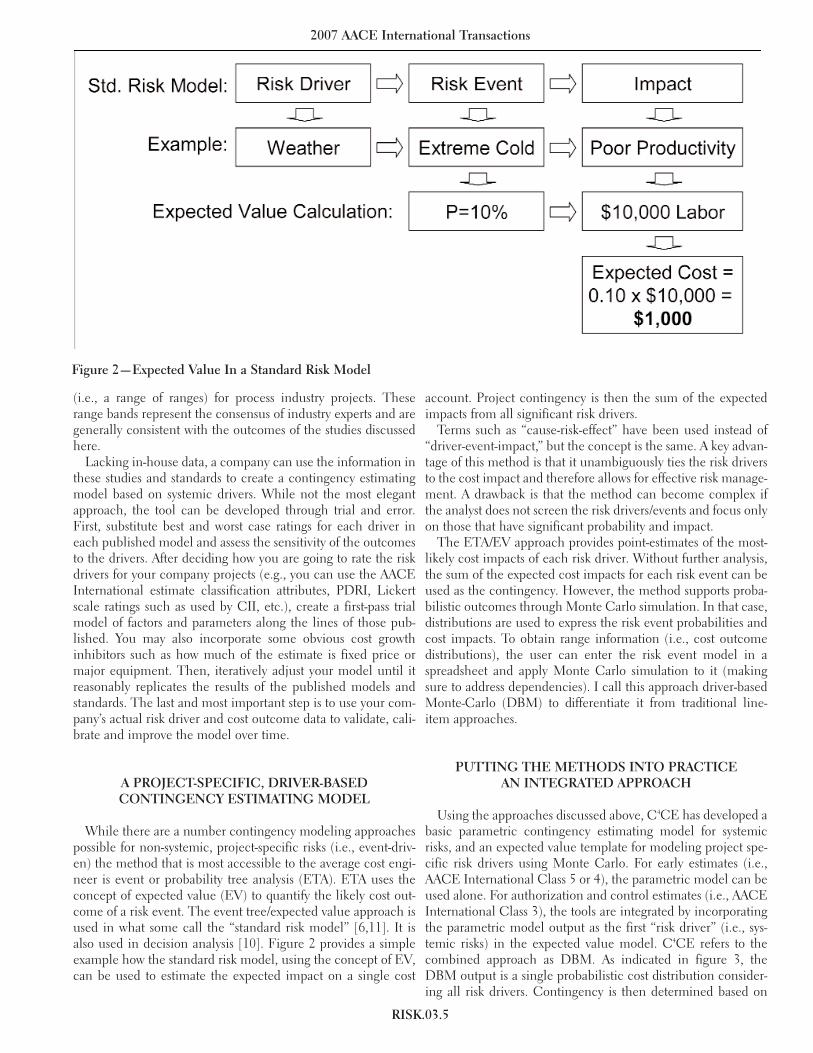
While there are a number contingency modeling approachespossible for non-systemic, project-specific risks (i.e., event-driv-en) the method that is most accessible to the average cost engi-neer is event or probability tree analysis (ETA). ETA uses theconcept of expected value (EV) to quantify the likely cost out-come of a risk event. The event tree/expected value approach isused in what some call the “standard risk model” [6,11]. It isalso used in decision analysis [10]. Figure 2 provides a simpleexample how the standard risk model, using the concept of EV,can be used to estimate the expected impact on a single cost

account. Project contingency is then the sum of the expectedimpacts from all significant risk drivers.

Terms such as “cause-risk-effect” have been used instead of“driver-event-impact,” but the concept is the same. A key advan-tage of this method is that it unambiguously ties the risk driversto the cost impact and therefore allows for effective risk manage-ment. A drawback is that the method can become complex ifthe analyst does not screen the risk drivers/events and focus onlyon those that have significant probability and impact.

The ETA/EV approach provides point-estimates of the most-likely cost impacts of each risk driver. Without further analysis,the sum of the expected cost impacts for each risk event can beused as the contingency. However, the method supports proba-bilistic outcomes through Monte Carlo simulation. In that case,distributions are used to express the risk event probabilities andcost impacts. To obtain range information (i.e., cost outcomedistributions), the user can enter the risk event model in aspreadsheet and apply Monte Carlo simulation to it (makingsure to address dependencies). I call this approach driver-basedMonte-Carlo (DBM) to differentiate it from traditional line-item approaches.

PUTTING THE METHODS INTO PRACTICEAN INTEGRATED APPROACH

Using the approaches discussed above, C4CE has developed abasic parametric contingency estimating model for systemicrisks, and an expected value template for modeling project spe-cific risk drivers using Monte Carlo. For early estimates (i.e.,AACE International Class 5 or 4), the parametric model can beused alone. For authorization and control estimates (i.e., AACEInternational Class 3), the tools are integrated by incorporatingthe parametric model output as the first “risk driver” (i.e., sys-temic risks) in the expected value model. C4CE refers to thecombined approach as DBM. As indicated in figure 3, theDBM output is a single probabilistic cost distribution consider-ing all risk drivers. Contingency is then determined based on

RISK.03.5


Figure 2—Expected Value In a Standard Risk Model

RISK.03.6


management’s desired level of confidence that the project willunderrun the cost.

The reason that the parametric model can be used alone forClass 5 and most Class 4 estimates is that for early estimates, thecost impacts of project-specific risks are relatively insignificantin comparison to systemic risk drivers. Also, given that the proj-ect scope is poorly defined for early estimates, project-specificrisk drivers are not readily definable. On the other hand, forwell-defined Class 3 or better estimates, the systemic risks (otherthan the use of new technology) tend to become less significantthan the project-specific risk.

In practice, the DBM method requires more explicit riskanalysis (i.e., risk identification, screening, and quantification)than the line-by-line approach; this is simply the price of usinga valid risk management method. A good practical reference onhow to do risk analysis is the recent text by Mulcahy [9]. First,after getting all the risk out on the table, the team must be selec-tive and explicit in defining the most probable and costly riskdrivers and events. Second, the team must quickly prepare con-ceptual (i.e., AACE International Class 5 quality) range esti-mates of each risk event’s impact. The method requires that therisk analysis team include some participants with expertise inthe key project execution roles (engineering, construction, etc),and some with conceptual cost estimating skills. Anotherrequirement is that the risk analysis be facilitated by someone

experienced with the approach so the team will surface the crit-ical risks without going overboard and getting lost in tangentsand details.

A unique element of the C4CE approach is the practical inte-gration of best practices. The practices themselves are docu-mented in the industry literature (re: this paper’s references)although most companies need some help putting it together.C4CE does not sell software; its mission is to help owner clientsbuild and implement their own core cost engineering capabili-ties in-house. Therefore, C4CE starts with basic contingencyestimating tool templates, customizes them to work with a com-pany’s estimating process (e.g., does the company use AACEInternational’s estimate classification matrix?, CII’s PDRIchecklists?, etc.), and develops risk analysis guidelines thataddress the company’s typical project risks. After some trainingin how to use the tool and conduct risk analysis, the owner com-pany has everything it needs in-house that it needs to put bestpractices for risk analysis and contingency estimating intoaction.

M onte-Carlo techniques for estimating contingency, astypically applied, are not working. They fail for threebasic reasons: users are not addressing dependencies

between model variables; they are not modeling the relation-

Figure 3—The C4CE’s DBM Method Integrates Best Practices

ships of risk drivers to cost outcomes (i.e., their methods are“line-item” driven); and they fail to recognize the differencesbetween systemic and project-specific risks. This paper providedreferences for and described a practical “driver-based” approachthat combines best practices for parametric modeling of sys-temic risk drivers and Monte-Carlo analysis of project-specificdrivers to produce reliable contingency estimates at all projectestimate phases. Hopefully, future research of the outcome ofindustry’s contingency estimates will show improving results asmethods such as these are incorporated.

REFERENCES1. AACE International, Recommended Practice No. 18R-97,

Cost Estimate Classification System—As Applied inEngineering, Procurement, and Construction for theProcess Industries.

2. Burroughs Scott E. and Gob Juntima, “ExploringTechniques for Contingency Setting”, AACE InternationalTransactions, 2004.

3. Hackney, John W. (Kenneth H. Humprhies, Editor),Control and Management of Capital Projects, 2nd Edition,AACE International, 1997.

4. Hollmann, John K., Editor, Total Cost ManagementFramework (Chapter 7.6 Risk Management), AACEInternational, Morgantown WV, 2006.

5. Hollmann, John K., Best Owner Practices for ProjectControl, AACE International Transactions, 2002.

6. Kaliprasad, Minnesh, Proactive Risk Management, CostEngineering, Vol 49, No 12, December 2006.

7. Kujawski, Edouard, “Why Projects Often Fail Even WithHigh Cost-Contingencies”, US Dept. Of Energy, Office ofScientific & Technical Information, Report# LBNL—51349, 2002.

8. Merrow, Edward W., Kenneth E. Phillips, andChristopher W. Meyers, Understanding Cost Growth andPerformance Shortfalls in Pioneer Process Plants, (R-2569-DOE), Rand Corporation, 1981.

9. Mulcahy, Rita, Risk Management, RMC PublicationsInc., 2003

10. Schuyler, John, Risk and Decision Analysis in Projects,Project Management Institute, 2001.

11. Smith, Preston G. and Guy M. Merritt, Proactive RiskManagement: Controlling Uncertainty in ProductDevelopment, Productivity Press, 2002.

12. Trost, Steven M. and Garold D. Oberlender, PredictingAccuracy of Early Cost Estimates Using Factor Analysisand Multivariate Regression, Journal of ConstructionEngineering and Management, Volume 129, Issue 2, pp.198-204 (March/April 2003)

John K. Hollmann, PE CCEOwner/Consultant

Validation Estimating, LLC47633 Weatherburn Terrace Sterling, VA 20165-4741, US

Phone: +1.703.945.5483Email: [email protected]

RISK.03.7


Needs For and Alternatives To KP/MH II-026c


SUBJECT: Scenario Development 1

2




6






12








20

QUESTION: 21

Please relate the probability distribution curve to the values and assumptions used in the 22

scenario development namely the Capital Cost High 30%, Reference 50%, and Low 20% cases 23

used in Chapter 10 of the NFAT submission. 24

25

RESPONSE: 26

For all capital costs (Hydroelectric generation, gas fired generation, wind generation, etc.) 27

techniques, including Monte Carlo analysis, were used in the initial development of the High 28

and Low estimates at the P10 and P90 levels and reference case at P50. These values, 29

statistically, correspond to probabilities of 25-50-25 for the scenarios (note this excludes the 30

impact of escalation). These probabilities were then refined to the 20-50-30, used for capital 31

cost cases, due to the following factors: 32

Needs For and Alternatives To KP/MH II-026c


Capital cost estimates for Keeyask G.S. and Conawapa G.S. are at an advanced stage; 1

nevertheless, costs are more likely to increase than decrease, mainly due to labour 2

costs. 3

Capital cost estimates for the natural gas-fired and wind generation alternatives are at 4

an earlier stage than those for Keeyask G.S. and Conawapa G.S. and likely do not capture 5

all cost risks. 6

There is a large amount of empirical data that supports the trend that costs are more 7

likely to increase than decrease for any capital project. 8

9

Please refer to Appendix 9.3 – Economic Evaluation Documentation of the NFAT submission for 10

full details (see specifically section 2.3.3 of Appendix 9.3) 11

Needs For and Alternatives To KP/MH II-027


SUBJECT: CEF Breakdown 1

2

REFERENCE: CEF 2009-2013 3

4

QUESTION: 5

Please fill in the attached table to ensure we are working with the correct values. 6

7

RESPONSE: 8

The response to this Information Request includes Commercially Sensitive Information and has 9

been filed in confidence with the Public Utilities Board. 10

Documents

Please provide the probability distribution curve used to ... Round 2.pdf · RISK.03.2 2007 AACE International Transactions. field labor costs; if field labor costs come in high,