Playing Easy or Playing Hard to Get:

When and How to Attract FDI∗

Thomas A. Gresik,† Dirk Schindler,‡ and Guttorm Schjelderup§

July 2020This version June 25, 2021

Abstract

We study the link between a country’s institutional quality in tax collection and its optimal cor-

porate tax policies in a model of heterogeneous multinationals that can shift income using both

debt and transfer prices. Countries with weak institutional quality can be made worse off adopting

policies that attract FDI as the benefits from higher wages and production are more than offset by

tax base erosion. Countries with moderate institutional quality can gain from under-utilizing their

ability to collect taxes, since the benefit of attracting more FDI outstrips the benefit of increased

tax revenue. Countries with very strong institutions benefit from FDI and should utilize their full

ability to collect taxes.

Keywords: FDI, thin capitalization rules, transfer pricing, institutional quality

JEL Classifications: F23, H26, H32, F68

∗We thank Rick Bond, Evelina Gavrilova, Mick Keen, Mohammed Mardan, Floris Zoutman and participants atthe Oxford University Centre for Business Taxation seminar for comments. Gresik acknowledges support from theInstitute for Scholarship in the Liberal Arts at the University of Notre Dame.†University of Notre Dame, Norwegian Center for Taxation, and CESifo, tgresik@nd.edu‡Erasmus School of Economics, Norwegian Center for Taxation, and CESifo, schindler@ese.eur.nl§Norwegian School of Economics, Norwegian Center for Taxation, and CESifo, guttorm.schjelderup@nhh.no

1 Introduction

Policymakers around the world perceive foreign direct investment (FDI) as beneficial for economic

development, tax revenue, income growth, and employment. The literature on inbound FDI docu-

ments welfare gains for host countries (e.g., Bernard, Eaton, Jensen, and Kortum (2003) and Melitz

(2003)), gains that exceed traditional gains from trade (Ramondo and Rodrıguez-Clare (2013)). At

the same time, the literature has largely neglected welfare losses from international tax avoidance,

despite the fact that OECD (2013) argues that it is a major concern. Tørsløv, Wier, and Zucman

(2018), for example, estimate that close to 40% of multinational profits are shifted to tax havens

each year. The amount of tax avoidance can be extreme. De Simone, Klassen, and Seidman (2017),

Dharmapala and Hebous (2017), Bilicka (2019), and Johannesen, Tørsløv, and Wier (2020) provide

evidence of a significant percentage of affiliates in both developed and developing host countries

that report zero (or negative) taxable income. According to Crivelli, de Mooij, and Keen (2016),

tax revenue losses from base erosion amount to 1% of GDP in developed countries and 1.5% of

GDP in developing countries. For developing countries, World Bank Group (2018) estimates fiscal

losses from tax avoidance as high as 5.9% of GDP.

In this paper, we derive the optimal corporate income tax policy for a host country in a model

that captures the net welfare benefits of inbound FDI in the presence of tax avoidance opportunities

and ask two normative questions: Is it beneficial for all countries to attract FDI when multinationals

can avoid taxes and shift (possibly all) income to tax havens? And, how does a host country’s

institutional quality in tax administration influence its optimal corporate tax policies? Institutional

quality is a dimension, in our model and in the world, along which host countries differ, especially

between and among developing and developed countries. In our model, a host country’s optimal

tax policy differs with its level of institutional quality and the ability of firm’s to avoid all corporate

income taxes. Moreover, the predicted variation in optimal tax policies is reflected in the data on

host country corporate tax policies.

By institutional quality we refer to a property of a host country’s tax revenue administration

that affects its ability to audit and counter income shifting by multinationals. Consistent with

the empirical results in Johannesen, Tørsløv, and Wier (2020) regarding tax revenues, we show

that host countries with weak institutional quality have less ability to use their corporate income

1

tax code to realize welfare gains from inbound FDI for reasons associated with lower reported

subsidiary income. For all host countries, FDI increases welfare via higher wages but higher wages

also reduce welfare through lower domestic profit. In addition, income shifting reduces welfare by

exporting tax revenues to foreign investors. In host countries with weaker institutional quality,

multinationals can shift more taxable income out of the host country thereby increasing corporate

tax revenue losses. Policies such as investment tax credits (ITCs) exacerbate this income shifting

problem, even if the credits are non-refundable, because they reduce an affiliate’s host tax liability.

They effectively shift income out of the host country equal to the pre-tax value of the credits before

the multinational engages in any income shifting via debt financing and transfer prices.1

We identify conditions under which a country’s welfare costs of FDI outweigh its benefits.

Perhaps paradoxically, we also show that among countries for which FDI improves welfare, some

countries can actually increase welfare from FDI by under-utilizing their ability to correct abusive

income shifting. These countries have intermediate levels of institutional quality and they gain

from attracting more FDI by not fully utilizing their ability to curb income shifting.

Our results are obtained in a model of national welfare maximization, multinationals with het-

erogeneous fixed entry costs, and immobile domestic firms. Multinationals can shift income with

both transfer prices and internal debt, the two most commonly used instruments to reduce tax

payments. We allow the host country to choose its corporate income tax rate, a thin capitalization

rule to limit income shifting by excessive interest deductions, and the intensity with which transfer

prices are audited. Most previous studies of the welfare effects of income shifting have only con-

sidered the use of debt to shift income (e.g., Hong and Smart (2010)) or non-specific methods of

income shifting (e.g., Slemrod and Wilson (2009) and Wang (2020)).2,3

Our analysis is novel in four main ways. First, we consider the welfare effects of a host country’s

corporate tax policies in the presence of both debt financing and transfer pricing. Second, we

1With an ITC, the multinational has less host tax to avoid. Thus, it will avoid at least as much host tax liabilityby coupling income shifting with an ITC than it would without an ITC. This effect means ITCs complement lax thincapitalization rules by making more tax avoidance feasible. ITCs can also apply to property or payroll taxes. AddingITCs to our model complicates the analysis without modifying the main conclusions of our analysis regarding theextensive margin and intensive margin effects of thin capitalization rules and transfer price enforcement.

2Gresik and Nelson (1994) derive optimal transfer price regulations but do not focus on the role of FDI or taxhavens.

3Heckemeyer and Overesch (2017) find that both channels are important with the effect of transfer pricing on thesemi-elasticity of profits with respect to international tax differentials being four times higher than the one of debtshifting.

2

model fixed costs for setting up a subsidiary in a host country and allow these costs to vary among

multinationals. This feature allows us to capture both intensive and extensive margin effects of

corporate income tax policy on FDI.4 Third, we explicitly account for the role of affiliates that

report zero taxable income because the marginal tax benefits of income shifting generally cease at

this point. Fourth, we endogenize the host country’s decision regarding how much of its institutional

quality to utilize in deterring tax avoidance.

A key discovery in our analysis pertains to how transfer pricing and debt financing combine

to affect a host country’s welfare from inbound FDI and the domestic economy. Permissive thin

capitalization rules move the corporate income tax closer to a cash flow tax and encourage an

increase in FDI because more host income can be shifted to tax haven affiliates. In effect, host

governments can discriminate more between investment sources, subjecting relatively immobile

domestic investment to higher tax rates than the highly mobile international investment.5 However,

permissive thin capitalization limits can also facilitate more aggressive transfer pricing on the

interest rate paid by the host subsidiary. With both instruments at their disposal, multinationals

can use transfer pricing to shift supernormal profits. A country with weaker institutional quality,

all else equal, will attract more FDI because each multinational can use its transfer prices to shift

more income out of the host country than will a country with stronger institutional quality. With

more FDI, the weaker country experiences higher wages but also reduced domestic profit. With

lower tax revenues paid by the domestic sector and the subsidiaries, weaker institutional quality in

tax revenue administration can result in larger welfare losses from transfer pricing than in countries

with stronger institutional quality.

It follows from our analysis that the welfare consequences of attracting FDI through corporate

tax policy can vary across countries, and this variation in consequences can lead to qualitatively

different tax policies, especially among developing, emerging, and developed countries. Developing

countries are characterized by a large informal sector, reliance on a small number of large firms

for tax revenue, and scarce tax administration resources.6 For developing countries, sufficiently

4Gresik, Schindler, and Schjelderup (2017) examined the interplay between debt financing and transfer pricing ina model with a representative multinational. That paper focused on the optimal design of thin capitalization rulesholding the host country tax rate constant.

5This view has been advocated by Hines (2010, p 120) who states, “tax avoidance opportunities presented bytax havens allow other countries to maintain high capital tax rates without suffering dramatic reductions in foreigndirect investment.”

6Developing countries are reliant on corporate tax revenue to fund basic infrastructure. Corporate tax revenue

3

permissive tax policies are needed to attract FDI, but this may be a bane rather than a boon.

Emerging economies may have better quality in tax revenue administration and may benefit from

attracting FDI if the tax base erosion can be partly curtailed. Developed countries, in contrast,

stand to gain from FDI as they in general have more advanced tax administrations.

Our finding that pursuing FDI can reduce a country’s welfare if its institutional quality is weak

is in line with concerns voiced by non-governmental organizations over the possibility that FDI

may be a burden to a country if multinationals can strip out most of the benefits of FDI and that

developing countries may be especially vulnerable. For example, OECD (2002) documents in a

meta-study that the benefits of FDI hinge on appropriate host country policies and a basic level of

development in a country. Several empirical studies also support our findings. They indicate that

the net effect of FDI depends on country characteristics, particularly the strength of local financial

markets and institutional quality.7 Acemoglu, Johnson and Robinson (2001), for example, estimate

that, if a country initially lies in the 25th percentile for institutional quality, and can improve its

institutions so that it moved into the 75th percentile, national income would be increased sevenfold.

Our results showing how optimal host country tax policies can differ with institutional quality

are also consistent with observed policies. In 2018, 42 countries used a safe harbor rule that imposed

a debt to equity (or asset) ratio above which interest payments on debt are no longer tax deductible.

The limits ranged from 0.5 to 0.8. In contrast, 95 (mainly developing) countries imposed no limit

which is effectively a safe harbor limit of one.8 Figure 1 plots the 2018 corporate tax rates and

safe harbor limits for non-OECD countries (excluding 11 tax haven countries that all have zero tax

rates and safe harbor limits of one). A notable feature of the data is the 20 percentage-point gap

or bifurcation between countries that have no thin capitalization limit (or a limit of 1) and those

that have lower safe harbor limits starting at 0.8. This bifurcation arises in our model because

of a natural non-convexity in equilibrium country welfare due to the change in the tax benefits of

makes up more than 25 percent of total tax revenue in developing countries, a number in stark contrast to developedcountries where the comparable number is 3-4 percent, see Avi-Yonah (2016). A significant informal sector (e.g., seeDharmapala, Slemrod, and Wilson (2011)) and weak institutional quality make it difficult for these countries to relyon personal income tax revenues instead of relying heavily on domestic firms. For example, Fjeldstad and Moore(2008) report that 286 domestic companies contribute about 70 per cent of domestic tax revenue in Tanzania.

7See Alfaro and Chauvin (2018) for a survey of how financial markets matter for the benefits of FDI.8In addition, 23 predominately OECD countries used an earnings stripping rule that imposes a maximum limit

on interest payments to earnings, with limits ranging from 10% to 60%. Five countries used a combination of safeharbor and earnings stripping rules and four countries used some other type of rule. Data was collected from EY(2018) and is available from the authors on request.

4

Figure 1: Safe Harbor Limits and Tax RatesData collected from EY (2018). The figure includes data from all non-OECD countries with safeharbor rules or no thin capitalization rule except for tax haven countries. Tax haven countriesare defined as countries with a zero corporate tax rate and no thin capitalization limit: Bahamas,Bahrain, Bermuda, Bonaire, BVI, Cayman Is., Guernsey, Isle of Man, Jersey, Maldives, and UAE.

income shifting that occur when affiliates have zero taxable income. As a result, a host country

that benefits from attracting FDI must choose between two distinct policies that are each locally

optimal: one that generates taxable income from the FDI and one that does not.9 Our paper is

the first to provide an economic explanation for this pattern in the data.

Developed countries tend to have advanced tax administrations to curb aggressive transfer pric-

ing while attracting welfare-enhancing FDI. The optimal policy for these countries is a combination

of moderate thin capitalization limits and moderate tax rates as reflected in the data. In equilib-

rium, these countries attract FDI that generates strictly positive taxable income. At the other end

of the institutional quality spectrum, developing countries tend to have weak tax administrations.

Conditional on attracting FDI, the optimal tax policy for these countries encourages aggressive

income shifting by setting a high thin capitalization limit and a high tax rate, whose burden falls

only on domestic firms (consistent with Hines (2010)). The result is FDI that attracts no taxable

income. Emerging countries tend to have intermediate levels of institutional quality. Some of these

countries will be close to indifferent between the moderate policies used by developed countries and

the aggressive income shifting policies of developing countries. As a result, two similar countries

can have very different optimal policies.

9Depending on the database, 20-50% of affiliates report non-positive tax bases. In our one-period model, thereare no tax benefits from generating negative taxable income by an affiliate but there can be in a multi-period setting.See also footnote 17.

5

A second empirical observation is that some countries with good institutional quality, such as

Austria, Ireland, Israel, and Sweden, have thin capitalization rules that our theory would associate

with low quality countries. The ability of a host country to choose the level of institutional quality

it applies to deterring tax avoidance reconciles the policies of the above countries with our model’s

predictions. If a country’s optimal policy when it uses its full institutional quality collects modest

or no tax revenues from subsidiaries, then under-utilizing its institutional quality will attract more

welfare-enhancing FDI and sacrifice little or no tax revenues from subsidiaries.10 Thus, a country

that prefers moderate tax policies when fully utilizing its institutional quality can earn greater

welfare by under-utilizing its institutional quality and being less aggressive in curbing income

shifting. We believe the result that countries with intermediate levels of institutional quality can

benefit from under-utilization is new to the FDI literature.

In section 2, we discuss the related literature. We set up the model in section 3. A motivating

example is presented in section 4. Equilibrium firm choices for each possible host country policy

are derived in section 5. In section 6, we analyze a host country’s optimal tax policy, and identify

when a country would choose to under-utilize its institutional quality. We extend our analysis to

consider earnings stripping rules in section 7, and offer concluding remarks in section 8.

2 Literature review

Our study is related to the literature on the welfare effects of FDI. There is a large literature that

spans several topics and it is outside the scope of this paper to review this literature. We shall

therefore concentrate our review on those papers that are most closely related to our study.

Our paper can be seen as part of the literature that studies how corporate income tax policies

affect welfare when multinationals can shift income to tax havens. Most of this literature suggests

that tax havens lower welfare. For instance, Slemrod and Wilson (2009) prove that the net welfare

advantage to attracting FDI in the presence of tax havens disappears when the host country can

charge domestic investors and foreign investors different tax rates, and workers can avoid wage taxes.

In their model, tax havens limit the power of a host country to tax the normal return on investment

and reduce its ability to indirectly tax workers. Positive welfare effects from tax havens are found in

10Stronger countries will not choose to under-utilize their institutional quality because they would lose too muchsubsidiary tax revenue.

6

Desai, Foley and Hines (2006) who argue that while tax havens may allow multinationals to reduce

income taxes paid in high-tax jurisdictions, they may have offsetting effects on real investment that

are attractive to the same governments. This argument is based on the insight that when capital

is perfectly mobile, a source tax on capital falls on immobile factors of production (Gordon, 1986).

The reason is that capital outflows following a tax increase lower worker productivity and thus

wages. From a policy point of view, it is therefore better to tax workers directly. Tax havens may

thus help firms avoid the tax on mobile capital partly or wholly, and reduce the adverse effects of

inefficient policies. Wang (2020) estimates the welfare effects of corporate taxes in the presence

of non-specific income shifting but treats income shifting as orthogonal to the output decisions of

subsidiaries and assumes away full income shifting. Spencer (2020) models the effect of repatriation

taxes, but allows for no income shifting.

Hong and Smart (2010) use a general equilibrium model to show a host country can benefit from

adopting tax policies that attract FDI by allowing multinationals to shift some of their income to a

tax haven. In their model, an affiliate of a multinational can be financed partially with debt issued

at the market (normal) interest rate from a related affiliate in a tax haven. In their model, there is

no role for transfer pricing on the interest rate, no firm heterogeneity, or no accounting for negative

taxable income. Since interest expenses under the thin capitalization limit are tax deductible,

internal debt reduces the multinational’s after-tax cost of capital and leads the multinational to

increase its overall capital investment in the host country. Increased investment increases the

demand for labor, which in turn increases the host wage rate and host welfare. The same forces

are present in our model. In the absence of agency costs from internal borrowing, Hong and Smart

(2010) show that the optimal policy of any host government is to allow the affiliate to be financed

entirely by debt by setting a thin capitalization limit of one. This prediction is inconsistent with the

many countries in Figure 1 that set lower limits. In the presence of agency costs, the optimal policy

is for all host countries to set a limit strictly less than one. This prediction is also inconsistent with

the variation in Figure 1. In contrast, by introducing differences in the ability of countries to deter

income shifting, our model is able to generate the range of thin capitalization limits observed in

the data

Besides Hong and Smart (2010), there is scarce theoretical literature on the optimal design

7

of thin capitalization rules.11 Haufler and Runkel (2012) study tax competition equilibria when

countries compete in tax rates and thin capitalization levels and countries can differ in population.

This paper does not include transfer pricing effects. Gresik et al. (2017) and Mardan (2017) study

the optimal choice of safe harbor vs. earnings stripping rules for a given corporate income tax

rate, with Mardan (2017) focusing on the role of capital market imperfections. Kalamov (2020a)

studies the choice of safe harbor vs. earnings stripping rules when host countries compete for FDI.

Kalamov (2020b) analyzes the Hong and Smart (2010) and the Gresik et al. (2017) models when

capital investment takes time. All of these papers assume a representative multinational. They

also ignore extensive margin effects and the effect of negative taxable income.

The model in Mardan (2020) is the closest to ours in the sense that it includes country variation

and it considers a country’s choice of the level of tax administration. Country variation is in the level

of economic development. Countries face the same cost of tax administration but firms operating

in less developed countries have higher capital costs. In contrast, in our model country variation

takes the form of differences in the capacity to audit income shifting. In Mardan’s model, firms

shift income in a non-specific manner rather than considering transfer pricing and debt financing

as separate but inter-connected channels. It also includes no labor, no firm heterogeneity, no entry

costs, and no negative income provisions. These last features are important because once one

accounts for the loss of tax benefits from income shifting when affiliate income is negative, an

equilibrium wage rate will not exist without entry costs or firm heterogeneity.

3 A model of income shifting via debt and transfer prices

There is a single host country whose economy consists of workers who inelastically supply one

unit of labor, a representative entrepreneur who owns a domestic firm, and possible multinational

activity. The domestic firm employs Ld units of labor at a wage rate w to produce G(Ld) units of

output that are sold in a competitive market. The production function G(·) is strictly increasing

and strictly concave in Ld. The pre-tax income of the domestic firm is

π = G(Ld)− wLd. (1)

11The empirical literature on thin capitalization rules has focused on their effects on capital structure (e.g., Buttneret al. (2012) and Blouin et al.(2014)) and the location of affiliates (e.g., Merlo et al. (2019)).

8

The host country levies a corporate income tax rate of t so the domestic firm has a post-tax profit

of (1− t)π.

There exist a continuum of multinational firms of mass one that maximize after-tax global profit

and are headquartered outside the host country. To introduce an extensive margin effect of host

tax policy, each multinational can choose to open an operating subsidiary in the host country by

incurring a fixed cost φ ≥ 0. The value of φ for a multinational is independently drawn from a

uniform distribution on [φ, φ], where 0 ≤ φ < φ. This variation in fixed entry costs is consistent with

the empirical evidence in Arkolakis (2010) and Eaton, Kortum, and Kramarz (2011). The operating

subsidiary is endowed with the production function F (lm, k), where lm denotes the amount of host

country labor it employs and k denotes the amount of capital invested in the subsidiary. F (·, ·) is

strictly increasing, strictly concave, and is homogeneous of degree η ∈ (0, 1) in capital and labor.

This last assumption implies that F exhibits decreasing returns to scale. The subsidiary pays the

same competitive wage rate as the domestic firm and sells its output in a competitive market whose

price is also normalized to one. Denote the multinational’s economic cost of capital by r.

All of the FDI is channeled to the host country subsidiary through a financing subsidiary

located in a tax haven, and takes the form of equity, E, and/or internal debt, B, so that k = E+B.

Following most corporate tax codes worldwide, we assume that interest expenses are tax deductible,

but costs of equity are not. For simplicity we do not allow the subsidiary to take on external debt,

although one of the determinants of the parent’s cost of capital may be the amount it borrows from

international markets.12 We assume that the multinational’s economic cost of capital reflects, in

part, a country-firm-specific risk of the investment so that r need not simply equal a worldwide

interest rate.13 The idiosyncratic cost of capital allows the multinational to charge its host country

subsidiary an interest rate R that can differ from r and implies that the multinational’s taxable

income in the host country, denoted by ΠT to distinguish pre-tax income from after-tax profit,

equals

ΠT = F (lm, k)− wlm −RB. (2)

12Davies and Gresik (2003) study the role of debt borrowed from host country investors.13While the norm in the tax competition literature is to assume all multinationals can finance investments at a

worldwide interest rate, our assumption is consistent with corporate finance textbooks that make clear that a firm’seconomic cost of capital varies with its CAPM β. In addition, the opportunity cost of investing in a host countrywill also depend on country-specific factors related to the multinational’s available projects in the host country andthe strength of the host country’s legal system.

9

That is, R is the transfer price of internal debt. Allowing the multinational to use its transfer price

on debt to shift income out of the host country is a simple and direct way to see the linkages between

debt shifting and transfer pricing. Moreover, disputes between tax authorities and multinationals

over interest rates charged between affiliates are commonplace in many countries.

The multinational incurs income shifting costs of C(R−r,B;α) = αc(R−r)B to reflect any tax

administration auditing the host country may conduct. These income shifting costs consist of three

components. First, the cost function c(·) is increasing and strictly convex in R− r, as we take r to

be the arm’s-length interest rate.14 Second, the multinational’s transfer price costs are proportional

to the amount of debt, as the total shifted income out of the host country will equal (R− r)B. The

transfer price costs are linear in B to coincide with the standard practice in most countries of using

a “comparable price” rule for ensuring that a company’s transfer price is effectively an arm’s-length

price. While the size of any non-compliance penalties is proportional to B, the auditing costs per

dollar of debt will depend on R − r in a non-linear way.15 Third, α > 0 captures reflects different

levels of auditing sophistication/intensity by the host country. In practice, α is chosen by a host

country to reflect marginal welfare benefits and costs of a stronger administration. Initially, we treat

α as an exogenous country characteristic reflecting its institutional capacity to administer its tax

code due to factors such as the quality of its court system or the level of corruption. Lower values

of α correspond to a country that faces higher marginal administrative costs or has less capacity to

audit transfer prices and impose non-compliance penalties. We then endogenize the host country

decision to under-utilize its institutional capacity and show that for some host countries the choice

of institutional quality is driven more by strategic factors than the direct marginal costs of building

quality.

A key reason for financing a subsidiary with debt instead of equity is that interest payments

on debt are tax deductible while equity payments are not. With the same rate applied to the

subsidiary’s host country income as is applied to the income of the domestic firm, the multinational’s

14If c(·) is linear, the multinational will either shift no income with R or the maximum amount possible. Thiswould make the firm’s transfer price independent of t, which is not consistent with the empirical evidence such asCristea and Nguyen (2016), Davies et al. (2018), and Flaaen (2017).

15Under the most common and preferred method among host countries, the comparable price auditing method,a revenue authority collects comparable price data from firms engaged in independent or arm’s-length transactions.An audited firm’s transfer price is typically deemed to be non-compliant if it falls outside the inter-quartile rangeof the comparable data. Thus, the probability that a firm is non-compliant, and subject to tax avoidance penalties,depends in an increasing way on the difference between a firm’s transfer price and its actual cost. See Gresik andOsmundsen (2008) for more details.

10

global after-tax profit equals

Π =

(1− t)ΠT +RB − rk − αcB − φ if ΠT ≥ 0

F − wlm − rk − αcB − φ if ΠT < 0.(3)

The first line of (3) is the sum of a multinational’s after-tax operating profit plus the net value of

the income it shifts into the tax haven, RB− rk−αcB, minus its fixed entry cost. The second line

of (3) reflects a host country policy that disallows a tax deduction for subsidiary losses. The term

−αcB still appears in this second line because transfer pricing remains costly for the multinational.

It just does not create any benefit once taxable subsidiary income is non-positive. Regardless of

the value of ΠT , the fixed entry costs are never tax deductible.16

Because shifting income is costly, the multinational in this case only shifts income until its

subsidiary has zero taxable income.17 Notice at fixed values of lm and k for which F−wlm−rk ≥ 0,

ΠT < 0 implies that Π is strictly decreasing in R for R > r. This means that at an optimum a

multinational will always set its transfer price so that ΠT ≥ 0.

To discourage multinationals from financing foreign operations entirely with debt, the host

country can adopt a thin capitalization rule. As indicated in the Introduction, the most common

choice is no rule at all followed by a safe harbor rule. Consistent with this usage and as in

Hong and Smart (2010) and Buttner et al. (2012), we model thin capitalization rules as the

maximum proportion, b, of a multinational’s capital investment for which interest expenses can be

tax deductible. The choice of b = 1 is equivalent to choosing no rule at all. For any b < 1, if the

multinational were to choose B > bk, where recall that k = E+B, the interest payments on B−bk

of the parent debt would not be tax deductible but the higher debt level would increase total transfer

price costs if R > r. Thus, this safe-harbor type of thin capitalization rule is equivalent to imposing

the constraint B ≤ bk on the multinational, except when the amount of debt is immaterial, as it

16Allowing φ to be tax deductible would not affect any of a multinational’s intensive margins and would onlyeliminate extensive margin effects at t = 1.

17In most countries, losses can be carried forward to offset taxable income in future years or they can be eventuallyrepatriated to the parent company. These options have no effect in a single period model. In practice, loss offsets arestill imperfect because they can expire and because they are not adjusted for inflation. Even in a dynamic model, thevalue to a firm of creating negative taxable subsidiary income is less than 100%. This is what our model captures.In addition, allowing for loss offsets increases the welfare costs of income shifting and makes it more likely that oursubsequent analysis would imply that a country should not attract FDI.

11

is when t = 0.18 After presenting our main results, we will discuss the implications of adopting an

earnings stripping rule in Section 7.

For t > 0, the cheapest income shifting option for the multinational is to shift income out of

the host country using only debt so that rB = F − wlm. Because the subsidiary operates under

decreasing returns to scale, this level of debt would have to be greater than or equal to k. Thus,

for any b ≤ 1 when t > 0, B = bk and the subsidiary’s debt-equity ratio equals b/(1− b). Except in

the limit case of b = 1 and constant returns to scale, the multinational will not be able to shift all

of its host country income to the tax haven with just debt. Thus, it will use both its debt financing

and transfer pricing options.19

The multinational’s problem then is to choose lm, k, and R to maximize

Π = (1− t)ΠT + k(Rb− r − αcb)− φ subject to ΠT = F − wlm −Rbk ≥ 0. (4)

A multinational with sufficiently large entry costs may choose not to enter because the multinational

can always guarantee itself zero global profit from its host country operations by not entering. By

the Envelope Theorem, there exists φ ∈ [φ, φ] such that multinationals with φ ≤ φ will enter

and those with φ > φ will not. Denote the measure of multinational firms that enter by M =

(φ−φ)/(φ−φ) and let Lm(b, t) and K(b, t) denote the quantities of labor and capital that maximize

(4), conditional on entry.20 These quantities will be independent of φ so aggregate multinational

labor demand equals MLm and aggregate FDI equals MK. Let R(b, t) denote a multinational’s

optimal transfer price and let Π∗(b, t, φ) denote the indirect profit of a firm with entry cost φ prior

to its entry decision.

Host country welfare is the weighted sum of labor income, after-tax domestic firm profit, and

tax revenues.21 Let βw ≥ 0 denote the welfare weight on domestic labor income and let 0 ≤ βπ ≤ 1

denote the welfare weight on after-tax domestic firm profit. We normalize the welfare weight on

18Adding a cost term to the firm’s profit function to reflect costs associated with the amount of debt a subsidiarytakes on would alter the way in which firms use their transfer price and the amount of debt to shift income withoutaltering the main economic trade-offs the host country faces because the cost function C(·) already captures someregulatory cost that are proportional to B.

19Including a cost of income shifting associated with a firm’s debt-equity ratio encourages even more reliance ontransfer pricing to shift income.

20Heterogeneity in terms of productive efficiency would generate a distribution of labor and capital demands acrossentrants but would not affect our main results.

21This is in contrast to studies such as World Bank Group (2020) that focus only on jobs benefits.

12

tax revenue to one. By assuming that βπ ≤ 1, we eliminate the desirability of subsidizing firms

with tax revenues. Thus, host country welfare is defined as

Ω = βww + βπ(1− t)π + tπ + t(F − wLm −RbK)M. (5)

The host country will choose its thin capitalization parameter b and its tax rate t to maximize its

welfare. If βw < 1 and βπ < 1 for a host country, then that country prefers a dollar of tax revenue

over a dollar of wage gains or after-tax domestic profit (see footnote 6). Our formulation allows us

to consider optimal tax policy for countries with a wide range of welfare functions including national

income maximization when βw = βπ = 1 and tax revenue maximization when βw = βπ = 0.

4 A motivating example

Before presenting our analysis of this model, we use an example to highlight several aspects of the

economic trade-offs in the model that generate two properties of host policies seen in Figure 1: The

mass of countries adopting no thin capitalization rule and the bifurcation gap between countries

with b < 1 and those with b = 1. Figure 2 graphs host country welfare as a function of the thin

capitalization parameter, b, for two slightly different host countries. For this example, we assume

F (lm, k) = k0.3l0.5m , so that the multinational sector generates rents. We also assume r = 0.08,

t = 0.45, α = 3, c(R − r) = (R − r)2, φ ∈ [0.1, 10], βπ = 0.3, and βw = 1. In the graph on the

left, G(Ld) = L0.85d . In the graph on the right, G(Ld) = L0.9

d , so that the domestic sector generates

fewer rents than in the graph on the left. These values are not meant to reflect calibrated values

but only to illustrate the range of possible welfare effects from different thin capitalization rules.

In both graphs, the observed welfare patterns due to changes in the thin capitalization limit are

due to three different multinational responses to a host country’s tax policy. First, the constant

welfare region corresponds to low values of b at which the host country attracts no FDI. The limited

amount of income shifting allowed via debt financing and transfer pricing is insufficient to permit

any multinational to cover its fixed cost of entry. Second, the middle region in which welfare is

quasi-concave in b corresponds to values of b at which the host country attracts strictly positive

levels of FDI and the subsidiaries report strictly positive taxable income. The quasi-concave shape

13

Figure 2: Host country welfare as a function of the thin capitalization parameter, b, when F (lm, k) =k0.3l0.5m , r = 0.08, t = 0.45, α = 3, c(R − r) = (R − r)2, φ ∈ [0.1, 10], βπ = 0.3, and βw = 1. In theleft graph, G(Ld) = L0.85

d . In the right graph, G(Ld) = L0.9d .

of the welfare function reflects a trade-off between the benefits of increased wage income from

multinational employment and welfare losses from lower domestic sector profits and lower domestic

and multinational tax revenues. Initially, increases in b attract enough FDI to generate a net

increase in welfare through wage increases. At some point, the wage gains from further increases in

b are not sufficient to outweigh the welfare losses, in part because of increases in marginal domestic

employment losses.22 Third, the strictly increasing region at high values b corresponds to tax policy

at which the host country attracts FDI but none of the subsidiaries report taxable income. They

are successful in shifting all of their income into the tax haven through a combination of transfer

pricing and debt financing. Host welfare is increasing in b in this last region as the gains from higher

wages dominate the truncated tax revenue losses from income shifting.23 The different regions of

multinational behavior result in two locally optimal values of b, at b = 0.66 and at b = 1. For the

graph on the left, the global optimum occurs at b = 1 while, for the graph on the right, the global

optimum occurs at b = 0.66.

In both graphs, the host country’s preferences are non-convex in b.24 Both an increase in b

above approximately 0.75 and a decrease in b below 0.75 increases host welfare. The non-convexity

arises because of the limitation on receiving a tax benefit from subsidiary losses and not because of

some technical assumption.25 As a result, a small decrease in the rents generated by the domestic

sector results in the optimal value of b jumping from 1 down to approximately 0.66.

22At low tax rates, one observes behavior consistent only with this region.23At very high tax rates, one can observe no FDI for low values of b and positive FDI with no taxable income for

high values of b. In this latter situation, welfare can be U-shaped.24Recall that convex preferences differ from a function being convex.25The exact value at the kink in the welfare function is slightly different in the two graphs.

14

5 Equilibrium firm choices

For each pair of policies (b, t), an equilibrium consists of an optimal labor, capital, and transfer

price choice for each multinational that chooses to enter, the set of entering firms defined by φ, an

optimal labor choice for the domestic firm, and a market-clearing wage rate. We will denote these

equilibrium values by Lm(b, t), K(b, t), R(b, t), φ(b, t), Ld(b, t), and w(b, t). Since M is the measure

of multinational firms that enter, we will show for each (b, t), that the resulting equilibrium must

fall into one of three cases: (1) M > 0 and ΠT > 0, (2) M > 0 and ΠT = 0, and (3) M = 0. We

denote the sets of values of (b, t) associated with each of these cases by M++, M+0, and M0. For

example, M0 = (b, t)|M = 0. In cases 1 and 2, some multinational firms enter so the amount

of FDI is strictly positive. In case 1, the subsidiary pays a strictly positive host tax. In case 2,

all taxable income is shifted out of the host country so the subsidiary pays no host tax. In case 3,

no multinational firms enter so there is no FDI in equilibrium for any (b, t) ∈ M0. Our goals in

this section are to describe the tax policies that generate each type of equilibrium and derive the

comparative statics associated with tax policy changes.

We begin by solving the multinational’s problem, (4), to choose Lm,K,R, and φ to maximize

aggregate multinational profit. The associated Lagrangian is

Λ = M(φ) [(1− t)ΠT +K(Rb− r − αcb)]−∫ φ

φ=φφdM(φ) + µM(φ)ΠT . (6)

The advantage of adopting this standard approach26 of maximizing aggregate profit is that it

transforms a discrete entry decision into a continuous optimization choice and makes it easier to

sign the model’s comparative statics.

The analysis of the multinational’s problem differs when t < 1 and when t = 1. We first analyze

optimal equilibrium choices when t < 1. With any positive-FDI equilibrium for which t < 1, the

first-order conditions associated with (6) imply

FL(Lm,K) = w, (7)

FK(Lm,K) =(µ− t)Rb+ r + αcb

1− t+ µ, (8)

26See Mas-Colell, Whinston, and Green (1995), section 5.E.

15

1− αc′ = 1− t+ µ, (9)

φ = (1− t)ΠT +K(Rb− r − αcb) + µΠT , (10)

and

µΠT = 0 (11)

where µ ≥ 0, FK denotes the marginal product of capital, and FL denotes the marginal product of

labor. While (7) implies that each multinational will equate its marginal product of labor with the

pre-tax wage rate, (8) implies that each multinational will equate its marginal product of capital

with its after-tax cost of capital. When the subsidiary’s taxable income is positive, (9) implies that

each multinational would like to set its transfer price to equate its marginal tax savings, t, with its

marginal cost of income shifting, αc′. If this transfer price implies negative taxable income, each

multinational will adjust its transfer price so that it is closer to r. In either situation, (9) shows that

the profit gain from income shifting, net of income shifting costs per dollar of debt, R−αc, is always

positive. This net gain is equal to r when R = r and is increasing in R as long as the marginal cost

of transfer pricing, αc′, is less than one. Eq. (10) implies that the marginal multinational to enter

will earn zero after-tax global profit. Eq. (11) is the standard complementary slackness condition.

When t = 1, each multinational benefits only from income shifted to the tax haven. Its profit

net of financing (r) and income shifting costs (αcb) equals K(Rb − r − αcb). Per unit of capital,

this net income shifting profit is maximized when R solves αc′ = 1, which we denote by R∗(1). In

order for a multinational to be willing to invest in the host country, its optimal net income shifting

profit must be greater than or equal to its fixed entry cost, φ. Define b = r/(R − αc) at R∗(1) as

the value of b ≤ 1 for which a multinational’s optimal net income shifting profit is zero.

If t = 1 and b ≤ b, then K = Lm = 0 because the net profit from shifted income is non-

positive. While the optimal transfer price reduces a multinational’s after-tax cost of capital below

r, it does not shift enough net income, Rb − αcb, to generate positive net income shifting profit.

No multinational will enter because none will be able to cover the fixed cost of entry.27 As the

host country’s institutional capacity improves to the point where it can detect any transfer price

deviation, so that α goes to∞, then R∗(1) goes to r and b goes to 1. In this case, every multinational

27If for some b ≤ b, R∗(1) implies ΠT < 0, a firm would have to choose a smaller value of R. Any R < R∗(1)would lower Π and still result in no entry.

16

would set a transfer price equal to its cost of capital. For any b, optimal net income shifting profit

when α tends to∞ converges to rK(b−1), which is non-positive and discourages any FDI at t = 1.

If t = 1 and b > b, a multinational earns strictly positive net income shifting profit on each

unit of capital. If it could, a multinational would invest an infinite amount of capital just to shift

income out of the host country. However, for a large enough value of K, the subsidiary’s taxable

income is strictly negative, i.e., ΠT < 0. Thus, a multinational that enters would choose values of

K, Lm, and R that imply ΠT = 0, FL = w, and µ = 1−αc′ > 0. With a strictly positive multiplier

on the non-negative taxable income constraint, the optimal transfer price will be strictly less than

R∗(1). As the host country’s institutional capacity to detect transfer price deviations, α, goes to

zero, R∗(1) goes to∞ and b goes to zero. In this case, with any positive value of b the host country

is unable to deter transfer prices that shift all subsidiary income out of the host country. Even with

shifting all taxable income out of the host country, a multinational may still not be able to earn

sufficient net income shifting profit to cover its fixed entry cost. We will address this issue below.

For all t, the remaining equilibrium conditions imply that the domestic firm employs labor until

the marginal product of labor equals the wage rate,

GL(Ld) = w, (12)

and that the labor market clears28,

Ld +M(φ)Lm = 1. (13)

Thus, a positive-FDI equilibrium with t < 1 is defined by the solution to (7) - (13). A no-

FDI equilibrium for t < 1 is defined by Lm(b, t) = K(b, t) = 0, φ(b, t) = φ, Ld(b, t) = 1 and

w(b, t) = GL(1). The value of R(b, t) is not relevant. For t = 1, the host tax is a pure profit tax in

the absence of FDI. We assume that the domestic firm maximizes its pre-tax income, in this case

so that the equilibrium is still defined by Ld(b, t) = 1 and w(b, t) = GL(1).

To ensure that each type of equilibrium arises for some tax policies, we make two assumptions:

(A1) F (Lm(0, 0),K(0, 0))− w(0, 0)Lm(0, 0)− rK(0, 0) > φ and

28Without heterogeneous firms, the tax loss restriction will imply generically that no market-clearing wage rateexists.

17

(A2) (R(1, 1)− r − αc(R(1, 1)− r))K(1, 1) > φ.29

Assumption (A1) requires that some multinationals enter when b = t = 0 and is sufficient for the

existence of tax policies in which case 1 equilibria arise. It will be satisfied if φ is small or if output

is sufficiently large. Assumption (A2) requires that some multinationals enter when b = t = 1.

Because b < 1, subsidiary taxable income will be zero. Assumption (A2) is sufficient for the

existence of tax policies in which case 2 equilibria arise as it ensures for b close to 1 that net income

shifting profit is large enough to cover the fixed entry costs for firms with φ close to φ. It defines

an upper bound on α because, as α goes to ∞, transfer price profit goes to 0 when b = 1. Thus,

there exists α <∞ such that for all α ≥ α,M+0 is empty. Together these two assumptions reduce

the set of tax policies that support zero FDI and make it less likely that the optimal tax policies

induce no FDI. Nevertheless, as we will show below, there always exist tax policies in which case

3 equilibria arise. The sets of tax policies that generate each type of equilibrium are illustrated in

Figure 3. It is constructed by analyzing multinational behavior for each type of equilibrium. We

now turn to this analysis.

Figure 3: Equilibrium Regions

29This assumption is equivalent to F (Lm(1, 1),K(1, 1))−w(1, 1)Lm(1, 1)−(r+αc(R(1, 1)−r))K(1, 1) ≥ φ becauseΠT = 0.

18

Case 1: Positive FDI and positive multinational tax revenues, M++

Assumption (A1) guarantees that this first type of equilibrium will exist for a positive measure

of tax policy parameters, b and t, because at t = 0, no multinational has an incentive to use its

transfer price to shift income, the amount of internal debt has no effect on multinational profit or

market equilibria, and global multinational profit is more than sufficient to cover the entry costs

when φ is close to φ. We have also shown above that this type of equilibrium cannot exist when

t = 1 so the following analysis only applies when t < 1. To understand multinational behavior in

this region, we need to understand how ΠT varies with respect to b and t. It turns out that the

response of firm behavior on M++ can differ when b ≤ b and when b > b. Thus, we will break our

analysis for Case 1 into two parts.

When ΠT > 0, µ = 0 so (8) implies that (1 − t)(FK − Rb) = r − Rb + αcb. The left-hand

side of the equation is the multinational’s marginal after-tax subsidiary income from FDI and the

right-hand side is the multinational’s net unit cost of capital, its unit cost of capital reduced by

its transfer pricing. For b ≤ b, each multinational’s adjusted cost of capital remains positive so

FK − Rb must be positive. For each b > b, if t = 0, R = r and r − Rb + αcb = r(1 − b) ≥ 0. The

adjusted cost of capital is non-negative. If t is close to one, then r − Rb + αcb < 0, which means

the tax haven affiliates report strictly positive income. Thus, for each b > b, there exists a value of

t, denoted by t1(b), at which r−Rb+αcb = 0. Eq. (8) then implies that FK −Rb > 0 for t < t1(b)

and FK −Rb < 0 for t > t1(b).

Furthermore, decreasing returns to scale of the subsidiary production function implies that

ΠT > FKK + FLLm − wLm −RbK = (FK −Rb)K. (14)

If FK − Rb ≥ 0, then (14) implies that ΠT must be strictly positive. Conversely, if ΠT = 0, then

FK−Rb must be strictly negative. Thus, for each fixed value of b ≤ b, ΠT must be strictly bounded

away from zero so the regions M++ and M+0 can only share a boundary when b > b. We refer to

this boundary as t2(b) in Figure 3. Before deriving this boundary, we first establish comparative

statics on M++ in Proposition 1. We use t and b subscripts on K, φ, w and R to denote the main

comparative statics.

Proposition 1 Assume (b, t) yields an equilibrium with strictly positive FDI and strictly positive

19

taxable subsidiary income. Then Kb > 0, φb > 0, wb > 0, Rb = 0, and Rt > 0. For b ≤ b, wt < 0

and if ΠT is sufficiently close to zero, then Kt < 0 and φt > 0. For b > b and t ≥ t1(b), Kt > 0

and φt < 0, and if ΠT is sufficiently close to zero, then wt > 0.

According to Proposition 1, weaker thin capitalization rules (larger values of b) attract more

capital and more multinationals (consistent with the estimates in Merlo et al. (2019)) and raise the

host wage. This happens because a larger value of b reduces the net cost of capital by allowing more

income shifting. However, tax rate changes have ambiguous effects. This ambiguity highlights the

importance of modelling the interactions between transfer pricing and debt financing.

For capital, the reason for the ambiguous effect can be seen by again focusing on (8). An

increase in t discourages capital investment by reducing the after-tax marginal product of capital

but it encourages capital investment by increasing the transfer price which lowers a firm’s income

shifting margin.

If b is small and taxable income, ΠT , is close to zero,30 income shifting reduces a multinational’s

net cost of capital but the tax haven profit (and marginal profit) remains negative as r−Rb+αcb > 0.

If it enters, a multinational will choose its amount of capital so that its marginal subsidiary profit

FK − Rb is positive. Although a higher tax rate decreases the after-tax cost of capital, (8) also

implies that FK = (r− tRb+αcb)/(1− t), where the expression on the right-hand side, the pre-tax

cost of capital, is increasing in t. Thus, the optimal amount of capital coincides with a larger

marginal product of capital and is achieved by less capital investment.

If b is large, income shifting now generates strictly positive marginal tax haven profit and implies

that a multinational will invest capital until its marginal taxable subsidiary income is negative. A

higher tax rate now encourages a multinational to increase its capital investment in order to shift

more aggregate income.

To understand the comparative statics results with respect to φ and w, notice that differentiating

(10) implies

dφ

dt= −ΠT − (1− t)Lmwt.

An increase in t directly reduces global after-tax multinational profit at a rate proportional to the

taxable income of subsidiaries and it generates a general equilibrium effect through the host wage.

30When ΠT is close to zero, the general equilibrium effects associated with income shifting will not dominatemultinational capital choices.

20

If taxable subsidiary income is close to zero, the equilibrium wage and equilibrium global after-tax

profit will change in opposite directions. When b is small, so that in equilibrium FK − Rb > 0,

income shifting opportunities are limited so the decrease inK for the same measure of multinationals

implies a lower wage. If ΠT is close to zero, the lower wage then encourages more multinationals

to enter. When b is large, so that in equilibrium FK − Rb < 0, the income shifting incentives to

increase capital investment increase global after-tax multinational profit. As long as ΠT is close to

zero, the wage will increase and global after-tax profit will decrease.

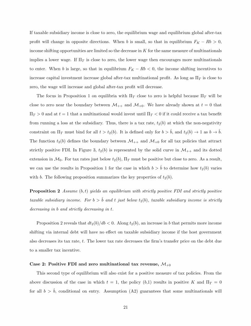
The focus in Proposition 1 on equilibria with ΠT close to zero is helpful because ΠT will be

close to zero near the boundary between M++ and M+0. We have already shown at t = 0 that

ΠT > 0 and at t = 1 that a multinational would invest until ΠT < 0 if it could receive a tax benefit

from running a loss at the subsidiary. Thus, there is a tax rate, t2(b) at which the non-negativity

constraint on ΠT must bind for all t > t2(b). It is defined only for b > b, and t2(b) → 1 as b → b.

The function t2(b) defines the boundary between M++ and M+0 for all tax policies that attract

strictly positive FDI. In Figure 3, t2(b) is represented by the solid curve in M++ and its dotted

extension inM0. For tax rates just below t2(b), ΠT must be positive but close to zero. As a result,

we can use the results in Proposition 1 for the case in which b > b to determine how t2(b) varies

with b. The following proposition summarizes the key properties of t2(b).

Proposition 2 Assume (b, t) yields an equilibrium with strictly positive FDI and strictly positive

taxable subsidiary income. For b > b and t just below t2(b), taxable subsidiary income is strictly

decreasing in b and strictly decreasing in t.

Proposition 2 reveals that dt2(b)/db < 0. Along t2(b), an increase in b that permits more income

shifting via internal debt will have no effect on taxable subsidiary income if the host government

also decreases its tax rate, t. The lower tax rate decreases the firm’s transfer price on the debt due

to a smaller tax incentive.

Case 2: Positive FDI and zero multinational tax revenue, M+0

This second type of equilibrium will also exist for a positive measure of tax policies. From the

above discussion of the case in which t = 1, the policy (b,1) results in positive K and ΠT = 0

for all b > b, conditional on entry. Assumption (A2) guarantees that some multinationals will

21

enter in equilibrium when (b, t) is close to (1,1). A multinational’s optimal choices in this region

no longer depend on t since each multinational sets its transfer price so that ΠT = 0. Thus,

Kt = Rt = φt = wt = 0 and Π∗(b, t, φ) = Π∗(b, t2(b), φ) for all t ≥ t2(b). The next proposition

summarizes the comparative statics on this region.

Proposition 3 Assume (b, t) yields an equilibrium with strictly positive FDI and zero taxable sub-

sidiary income. Then wb > 0 if M is close to zero. Kb and Rb are ambiguous in sign but φb > 0,

which means that multinational profit increases with b in this region.

For policies that attract FDI but result in no taxable subsidiary income, the multinational’s

global profit is equal to K(Rb − r − αcb). While an increase in the thin capitalization limit, b,

creates the incentive for multinationals to shift more income out of the host country per unit of

capital for the same transfer price, the fact that subsidiaries were already generating zero taxable

income means that, in order to increase income shifting profit, multinationals must adjust their

capital investments and transfer prices to maintain zero taxable income. Holding the wage fixed,

dΠT = 0 if (FK −Rb)dK− bKdR−RKdb = 0. Because FK −Rb < 0 for this case, a multinational

can maintain zero taxable income by increasing K, which reduces taxable income, and decreasing

R, which increases taxable income, or vice versa. Even with general equilibrium wage effects, one

of these options will increase global after-tax profit. Thus, an increase in b will increase global

after-tax profit and attract more multinationals.

Case 3: No FDI, M0

The above analyses of cases 1 and 2 were conditional on entry by multinational firms. In this

subsection, we will identify tax policies that attract no FDI. Tax policies that attract no FDI do

exist. At b = 0 and t = 1, Π∗ = −rK − φ < 0 so no firm will enter. This implies φ = φ or M = 0.

However, by (A1), multinational firms will enter at b = t = 0. Because Π∗ is continuous in t, there

exists 0 < t0 < 1 such that the host country attracts no FDI for all t ≥ t0 when b = 0 and it

attracts positive FDI for all t < t0, again when b = 0. The equilibrium analysis when t = 1 also

implies M = 0 for each b ≤ b. Because Π∗ is continuous in b, there exists a positive measure of

policies for which the host country attracts no FDI. We now turn to a more explicit analysis to

determine the boundaries of the set M0.

22

For all b ≤ b and t < 1, the above analysis of case 1 shows any multinational that enters will

earn ΠT > 0. Thus, for b ≤ b, the economy can only transition between equilibria with strictly

positive FDI and strictly positive taxable subsidiary income to equilibria with no FDI. From the

proof of Proposition 1, φb > 0 and, when M is close to zero, φt < 0. Thus, the boundary between

M++ andM0 must be strictly increasing. It is represented by the upward sloping curve in Figure

3.

Intuitively, smaller values of b encourage less capital investment and less entry. If there is no

FDI at (b, t), there should also be no FDI for all (b′, t) with b′ < b. Suppose that this result was not

true. That is, for some b′ < b, assume FDI is strictly positive. At (b, t), the lack of FDI means that

w(b, t) = GL(1). With strictly positive FDI at (b′, t), the equilibrium wage, w(b′, t) must exceed

GL(1) as otherwise the labor market would exhibit excess demand. Formally then

φ ≥ Π∗(b, t) ≥ Π(Lm(b′, t),K(b′, t), R(b′, t), w(b, t), b, t)

> Π(Lm(b′, t),K(b′, t), R(b′, t), w(b′, t), b, t) > Π(b′, t). (15)

The second weak inequality in (15) follows from profit maximization. The first strict inequality in

(15) arises because by assumption the reduction in b increases the equilibrium wage by attracting

FDI and the second strict inequality arises because a reduction in b holding the host wage and

all multinational choices fixed reduces multinational profit by allowing a smaller tax deduction for

interest payments. Together the chain of inequalities in (15) implies there will be no FDI at (b′, t),

which contradicts our initial assumption. A similar argument also applies to increases in t.

At b = b and for all t < 1, ΠT > 0, so in the limit as b converges to b from above, t2(b)

converges to one. In addition, in the limit as t approaches one with b = b, transfer price profits

go to zero and after-tax subsidiary profit goes to zero. These two results imply that for t close to

one, multinational profit will not be sufficient to cover the fixed cost of entry. Thus, the boundary

between M++ and M0 at b must occur at some t < 1 and it must continue into the region for

which b > b.

Finally, because t2(b) is decreasing by Proposition 2, there exists b0 > b for which no FDI arises

at (b0, t2(b0)). For t > t2(b0), the host economy moves into M+0, and the equilibrium firm choices

and the equilibrium wage become independent of t. With ΠT = 0, equilibrium multinational profit

23

also does not vary with t. As a result, the boundary of M0 will extend into the region where

ΠT = 0 and will be horizontal. By Proposition 3, M must be positive for b > b0.

A special case arises when transfer pricing is costless because α = 0. This is the case for which

the host country’s institutions are so weak that it cannot detect or chooses not to detect any transfer

price deviation. With α = 0, M0 = (0, t)|t ≥ t0 and M++ = (b, 0)|0 ≤ b ≤ 1 ∪ (0, t)|t < t0.

M+0 thus consists of all policies with b > 0 and t > 0. With no institutional capacity to limit

transfer price deviations, the host country will attract strictly positive FDI with any strictly positive

thin capitalization limit and any strictly positive tax rate but multinationals will shift all taxable

income out of the host country.

6 Optimal tax policies

Equilibrium host welfare is continuous in (b, t). This means a globally optimal tax policy will exist.

However, in order to identify the globally optimal policy we must identify a host country’s optimal

tax policy for each region in Figure 3 separately, and then compare host welfare at each of the local

optima to find the global optimum. Special attention will be paid to the changes in welfare near

the boundaries of the three regions because the local incentives will help identify non-convexities

in equilibrium host welfare.

For all three types of equilibria, totally differentiating (5) yields

dΩ = tΠTdM − tMbKdR+ tM(FK −Rb)dK − ((t+ (1− t)βπ)Ld − βw + tMLm)dw

− tMRKdb+ ((1− βπ)π + ΠTM)dt. (16)

Eq. (16) reveals that host welfare is increasing in its tax rate and the measure of multinational

firms that enter and decreasing in the transfer price and the thin capitalization limit. The effect of

a change in subsidiary capital and the host wage can be positive or negative.

Case 1: FDI > 0 and ΠT > 0

Denote the optimal tax policy onM++ by (b++, t++) and define Ω++ = Ω(b++, t++). Because

this case is defined by strict inequalities, an optimal policy on M++ need not exist as the host

country’s incentives may be to move out of this region.

24

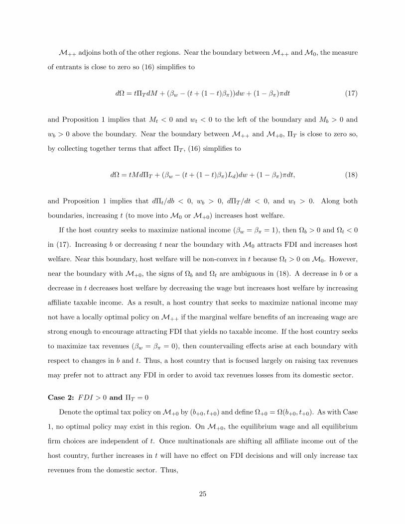
M++ adjoins both of the other regions. Near the boundary betweenM++ andM0, the measure

of entrants is close to zero so (16) simplifies to

dΩ = tΠTdM + (βw − (t+ (1− t)βπ))dw + (1− βπ)πdt (17)

and Proposition 1 implies that Mt < 0 and wt < 0 to the left of the boundary and Mb > 0 and

wb > 0 above the boundary. Near the boundary between M++ and M+0, ΠT is close to zero so,

by collecting together terms that affect ΠT , (16) simplifies to

dΩ = tMdΠT + (βw − (t+ (1− t)βπ)Ld)dw + (1− βπ)πdt, (18)

and Proposition 1 implies that dΠt/db < 0, wb > 0, dΠT /dt < 0, and wt > 0. Along both

boundaries, increasing t (to move into M0 or M+0) increases host welfare.

If the host country seeks to maximize national income (βw = βπ = 1), then Ωb > 0 and Ωt < 0

in (17). Increasing b or decreasing t near the boundary with M0 attracts FDI and increases host

welfare. Near this boundary, host welfare will be non-convex in t because Ωt > 0 onM0. However,

near the boundary with M+0, the signs of Ωb and Ωt are ambiguous in (18). A decrease in b or a

decrease in t decreases host welfare by decreasing the wage but increases host welfare by increasing

affiliate taxable income. As a result, a host country that seeks to maximize national income may

not have a locally optimal policy onM++ if the marginal welfare benefits of an increasing wage are

strong enough to encourage attracting FDI that yields no taxable income. If the host country seeks

to maximize tax revenues (βw = βπ = 0), then countervailing effects arise at each boundary with

respect to changes in b and t. Thus, a host country that is focused largely on raising tax revenues

may prefer not to attract any FDI in order to avoid tax revenues losses from its domestic sector.

Case 2: FDI > 0 and ΠT = 0

Denote the optimal tax policy onM+0 by (b+0, t+0) and define Ω+0 = Ω(b+0, t+0). As with Case

1, no optimal policy may exist in this region. On M+0, the equilibrium wage and all equilibrium

firm choices are independent of t. Once multinationals are shifting all affiliate income out of the

host country, further increases in t will have no effect on FDI decisions and will only increase tax

revenues from the domestic sector. Thus,

25

Proposition 4 For each b > b0, host welfare onM+0, where equilibrium subsidiary taxable income

is equal to 0, is maximized at t = 1.

Proof. By (16), Ωt = (1 − βπ)π > 0 for all βπ < 1 on M+0. For each b > b0, t = 1 maximizes

host welfare on M+0. If βπ = 1, then host welfare is independent of t on M+0 and t = 1 is still

optimal.

In light of Proposition 4, the optimal policy onM+0 must take the form (b, 1) for some b > b0.

Note however that the policy (b0, 1) attracts no FDI and is thus not an element of M+0.

With t+0 = 1, for any b > b0,

Ω+0(b) ≡ Ω(b, 1) = G(Ld) + (βw − Ld)GL(Ld) (19)

and

Ωb = (βw − Ld)wb. (20)

According to Proposition 3, wb > 0 when M is close to zero. For b just above b0, M is close to zero

and Ωb = (βw−1)wb < 0 for all βw < 1. In this case, the local incentives onM+0 lead to the policy

(b0, 1), which implies the host country prefers attracting no FDI in equilibrium to attracting a small

amount of FDI. In this case, we refer to (b0, 1) as locally optimal on M+0 ∪M0. Among policies

that attract FDI but generate no affiliate tax revenue, a necessary but not sufficient condition for

no optimal policy to exist is βw < 1. For example, this will be the case if the host country seeks to

maximize tax revenues (βw = βπ = 0).31

Proposition 5 The policy (b0, 1), which does not attract FDI, is locally optimal on M+0 ∪M0

when the host country has a smaller welfare weight on wage income than on tax revenues.

Proposition 5 highlights a welfare trade-off between wage income and tax revenues generated

by the domestic sector. A small increase in the thin capitalization limit above b0 attracts a small

amount of FDI and increases the equilibrium wage, which in turn reduces domestic taxable income

and hence also tax revenues collected from domestic firms. For host countries that value an extra

31Another example of a welfare function that puts less weight on wages than tax revenues is a Rawls welfarefunction for a host country with an unproductive group of residents who earn no wage income.

26

dollar of tax revenue even a little more than an extra dollar of wage income, the policy (b0, 1) is

locally optimal.

Even with βw < 1, a locally optimal policy onM+0 may exist if for large enough values of b the

multinational employs enough labor so that Ld < βw as this would imply Ωb ≥ 0. If a weak enough

limit attracts enough multinational employment, host welfare can be convex in b when t = 1. In

this case, a policy we will denote by (b′+0, 1) will be a local optimum even if there is no global

optimum on M+0. Figure 4 below provides an example of this possibility for which b′+0 = 1.

Case 3: M = 0

On M0, the equilibrium wage and all equilibrium firm choices are independent of b and t. By

increasing t, the host country can increase tax revenues from the domestic firm. Thus,

Proposition 6 For each b such that for some t the host country attracts no FDI, host welfare is

maximized at t = 1.

Proof. By (16), Ωt = (1− βπ)π > 0 for all βπ < 1 when (b, t) ∈ M0. If βπ = 1, then host welfare

is independent of t on M0. Thus, t = 1 is still optimal.

At t = 1, host welfare is independent of b on M0. Therefore, host welfare is maximized at

(b0, 1) and maximal host welfare on M0 is Ω0 ≡ Ω(b0, 1) = G(1) + (βw − 1)GL(1) > 0.

Comparing optimal policies in each case

The above welfare analysis identifies four distinct tax policies that can be or are local optima

for the host country: (b++, t++), (b+0, 1), (b′+0, 1), and (b0, 1). In this subsection, we proceed by

showing that attracting no FDI can be globally optimal for a host country, by showing how cross-

country differences in α can generates cross-country differences in tax policies, and by showing how

endogenizing the host country’s institutional quality parameter, α affects the (globally) optimal

host policy.

Figure 4 illustrates an example in which it is optimal for the host country to adopt a tax policy

that attracts no FDI. For this example, F (lm, k) = 1.5k0.3l0.4m , G(Ld) = L0.9d , r = 0.08, α = 3,

c(R − r) = (R − r)2, φ ∈ [0.1, 10], βπ = 0, and βw = 0.8. The values of λ, γ, δ and A are selected

to be suggestive of a developing country as these values are indicative of low domestic rents, high

subsidiary rent consistent with Karabarbounis and Nieman (2014), and a foreign sector that is

27

Figure 4: Host welfare as a function of b and t. No FDI is optimal when F (lm, k) = 1.5k0.3l0.4m ,G(Ld) = L0.9

d , r = 0.08, α = 3, c(R − r) = (R − r)2, φ ∈ [0.1, 10], βπ = 0, and βw = 0.8. t = 1 inthe right panel.

larger than the domestic sector. The remaining parameter values define a baseline example in

which it is optimal for the host country to attract no FDI. The left graph plots Ω against b and

t. The right graph plots Ω as a function of b for t = 1. Both graphs reveal non-convexities in the

host welfare function identified in the above welfare analysis. The right graph, in particular, shows

that an increase in b just above b0 ≈ 0.55 attracts FDI but the welfare gain from a higher wage

is smaller than the welfare loss from lower domestic firm tax revenues. For values of b closer to

one, welfare is increasing in b. For these values of b, domestic employment has fallen to the point

at which the marginal welfare gains from a higher wage now outweigh the marginal welfare losses

from lower domestic firm tax revenues. Even though welfare is locally maximized at (b, t) = (1, 1),

the globally optimal tax policy occurs at (b0, 1). It attracts no FDI in equilibrium.

Figure 5 illustrates an example in which it is optimal for the host country to adopt a tax policy

that does attract FDI. It is generated using the same parameter values used in Figure 4 except

that α = 2.13, βπ = 0.3, and βw = 0.85. The main change is the reduction in α. We chose these

specific parameter values to create an example in which the host country is close to indifferent

between all three local optima. We focus on this 3-way indifference case as it allows us to show

how a change in α can cause a host country’s optimal tax policy to shift between the three possible

equilibrium cases and generate the discontinuous jump in safe harbor limits we observe in Figure

1. Before discussing Figure 5 in more detail, as it is presented solely for illustration purposes, we

first compute and analyze two comparative statics with respect to changes in α that will help us

28

establish general results about how a small change in α can lead to a discrete change in tax policy.

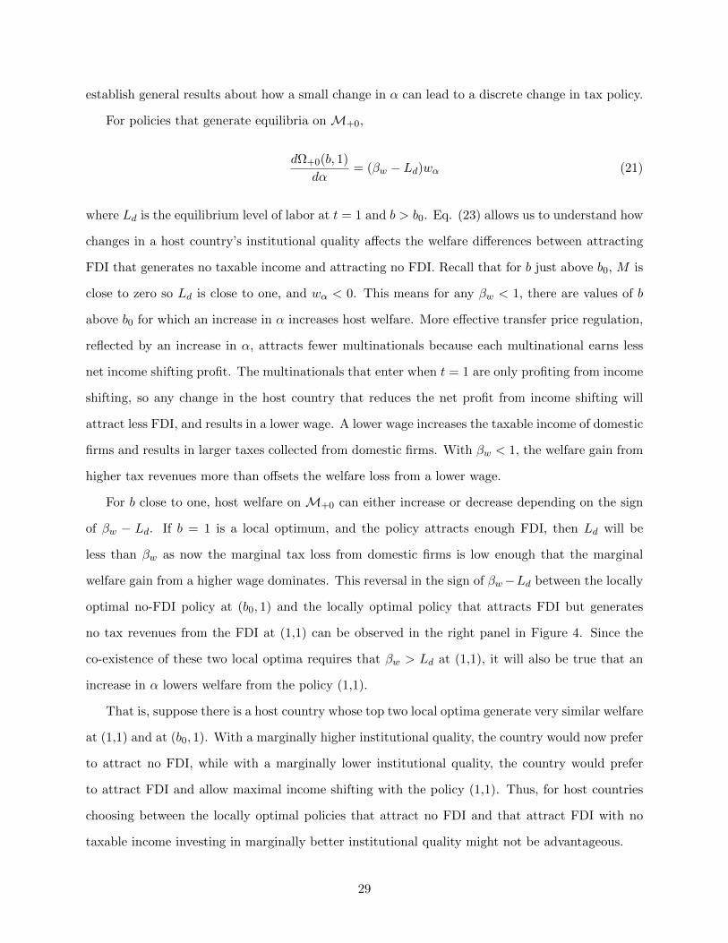
For policies that generate equilibria on M+0,

dΩ+0(b, 1)

dα= (βw − Ld)wα (21)

where Ld is the equilibrium level of labor at t = 1 and b > b0. Eq. (23) allows us to understand how

changes in a host country’s institutional quality affects the welfare differences between attracting

FDI that generates no taxable income and attracting no FDI. Recall that for b just above b0, M is

close to zero so Ld is close to one, and wα < 0. This means for any βw < 1, there are values of b

above b0 for which an increase in α increases host welfare. More effective transfer price regulation,

reflected by an increase in α, attracts fewer multinationals because each multinational earns less

net income shifting profit. The multinationals that enter when t = 1 are only profiting from income

shifting, so any change in the host country that reduces the net profit from income shifting will

attract less FDI, and results in a lower wage. A lower wage increases the taxable income of domestic

firms and results in larger taxes collected from domestic firms. With βw < 1, the welfare gain from

higher tax revenues more than offsets the welfare loss from a lower wage.

For b close to one, host welfare on M+0 can either increase or decrease depending on the sign

of βw − Ld. If b = 1 is a local optimum, and the policy attracts enough FDI, then Ld will be

less than βw as now the marginal tax loss from domestic firms is low enough that the marginal

welfare gain from a higher wage dominates. This reversal in the sign of βw−Ld between the locally

optimal no-FDI policy at (b0, 1) and the locally optimal policy that attracts FDI but generates

no tax revenues from the FDI at (1,1) can be observed in the right panel in Figure 4. Since the

co-existence of these two local optima requires that βw > Ld at (1,1), it will also be true that an

increase in α lowers welfare from the policy (1,1).

That is, suppose there is a host country whose top two local optima generate very similar welfare

at (1,1) and at (b0, 1). With a marginally higher institutional quality, the country would now prefer

to attract no FDI, while with a marginally lower institutional quality, the country would prefer

to attract FDI and allow maximal income shifting with the policy (1,1). Thus, for host countries

choosing between the locally optimal policies that attract no FDI and that attract FDI with no

taxable income investing in marginally better institutional quality might not be advantageous.

29

Second, on M++, the Envelope Theorem and the firm’s first-order conditions (7) - (10) imply

that

dΩ++(b++, t++)

dα= (βw − t− (1− t)βπLd)wα + tΠTMα−

t(Rb− r − αcb)1− t

Kα−tMbK(1− αc′)

1− tRα.

(22)

Direct calculations show that the comparative statics Kα, Rα, Mα, and wα are all negative. That is,

an increase in α reduces capital investment per firm, the transfer price, the measure of multinational

firms, and the host wage.

If b++, the optimal thin capitalization level on M++, satisfies ∂Ω++/∂b = 0, (22) can be

simplified by noticing that wα = x · wb, Mα = x ·Mb, and Kα = x · Kb for x = cb/(α(c − Rc′)).

Using the host country’s first-order condition on b then implies that

dΩ++(b++, t++)

dα= tMbK

(c′

αc′′− Rc

α(c−Rc′)

)> 0, (23)

due to the convexity of c(·). Thus, an increase in α increases host welfare from the locally optimal

tax policy that attracts FDI and results in strictly positive taxable income. The reason is that better

institutional quality in the tax authority encourages multinationals to shift less income out of the

host country. We can use this comparative static to understand how changes in a host country’s

institutional quality affects the welfare differences between the optimal policy that attracts FDI

and generates taxable income with the optimal policy that attracts no FDI or with the optimal

policy that attracts FDI and generates no taxable income.

In order for a small difference in a host country’s institutional quality to lead to a large change

in its optimal tax policy as suggested by Figure 1, consider the situation in Figure 5 in which

three distinct local optima exist (one of them at (1,1)) and yield identical host welfare. βw must

be less than one for this three-way tie scenario to exist. Welfare values are reported in Table 1.

The globally optimal tax policy attracts no FDI with b below approximately 0.4 and t = 1. If α

increases to 2.14, the globally optimal tax policy attracts FDI and generates taxable income by

setting b = 0.47 and t = 0.56.

According to comparative statics (21) and (23), if one begins with a host country whose value of

α implies it is indifferent among three distinct local policy optima, a host country with a marginally

30

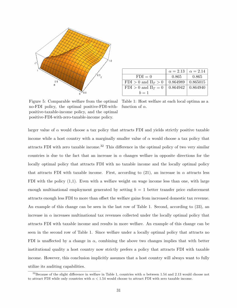
Figure 5: Comparable welfare from the optimalno-FDI policy, the optimal positive-FDI-with-positive-taxable-income policy, and the optimalpositive-FDI-with-zero-taxable-income policy.

α = 2.13 α = 2.14

FDI = 0 0.865 0.865

FDI > 0 and ΠT > 0 0.864989 0.865015

FDI > 0 and ΠT = 0 0.864942 0.864940b = 1

Table 1: Host welfare at each local optima as afunction of α.

larger value of α would choose a tax policy that attracts FDI and yields strictly positive taxable

income while a host country with a marginally smaller value of α would choose a tax policy that

attracts FDI with zero taxable income.32 This difference in the optimal policy of two very similar

countries is due to the fact that an increase in α changes welfare in opposite directions for the

locally optimal policy that attracts FDI with no taxable income and the locally optimal policy

that attracts FDI with taxable income. First, according to (21), an increase in α attracts less

FDI with the policy (1,1). Even with a welfare weight on wage income less than one, with large

enough multinational employment generated by setting b = 1 better transfer price enforcement

attracts enough less FDI to more than offset the welfare gains from increased domestic tax revenue.

An example of this change can be seen in the last row of Table 1. Second, according to (23), an

increase in α increases multinational tax revenues collected under the locally optimal policy that

attracts FDI with taxable income and results in more welfare. An example of this change can be

seen in the second row of Table 1. Since welfare under a locally optimal policy that attracts no

FDI is unaffected by a change in α, combining the above two changes implies that with better

institutional quality a host country now strictly prefers a policy that attracts FDI with taxable

income. However, this conclusion implicitly assumes that a host country will always want to fully

utilize its auditing capabilities.

32Because of the slight difference in welfare in Table 1, countries with α between 1.54 and 2.13 would choose notto attract FDI while only countries with α < 1.54 would choose to attract FDI with zero taxable income.

31

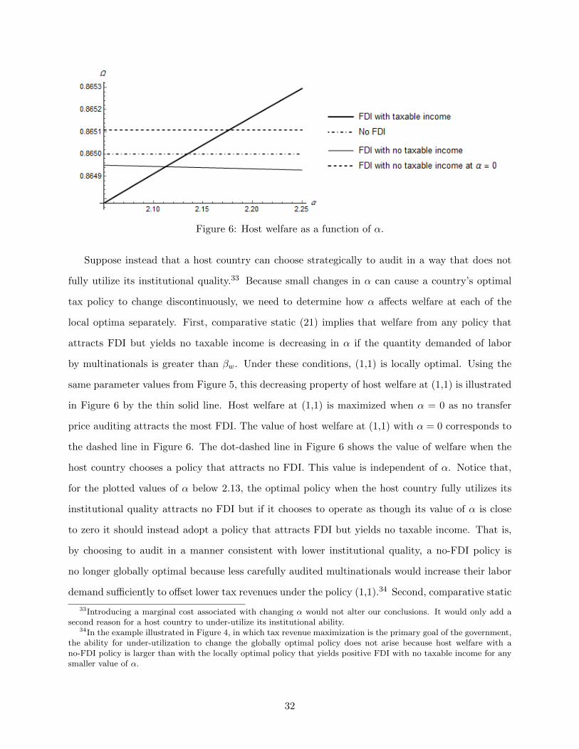
Figure 6: Host welfare as a function of α.

Suppose instead that a host country can choose strategically to audit in a way that does not

fully utilize its institutional quality.33 Because small changes in α can cause a country’s optimal

tax policy to change discontinuously, we need to determine how α affects welfare at each of the

local optima separately. First, comparative static (21) implies that welfare from any policy that

attracts FDI but yields no taxable income is decreasing in α if the quantity demanded of labor

by multinationals is greater than βw. Under these conditions, (1,1) is locally optimal. Using the

same parameter values from Figure 5, this decreasing property of host welfare at (1,1) is illustrated

in Figure 6 by the thin solid line. Host welfare at (1,1) is maximized when α = 0 as no transfer

price auditing attracts the most FDI. The value of host welfare at (1,1) with α = 0 corresponds to

the dashed line in Figure 6. The dot-dashed line in Figure 6 shows the value of welfare when the

host country chooses a policy that attracts no FDI. This value is independent of α. Notice that,

for the plotted values of α below 2.13, the optimal policy when the host country fully utilizes its

institutional quality attracts no FDI but if it chooses to operate as though its value of α is close

to zero it should instead adopt a policy that attracts FDI but yields no taxable income. That is,

by choosing to audit in a manner consistent with lower institutional quality, a no-FDI policy is

no longer globally optimal because less carefully audited multinationals would increase their labor

demand sufficiently to offset lower tax revenues under the policy (1,1).34 Second, comparative static

33Introducing a marginal cost associated with changing α would not alter our conclusions. It would only add asecond reason for a host country to under-utilize its institutional ability.

34In the example illustrated in Figure 4, in which tax revenue maximization is the primary goal of the government,the ability for under-utilization to change the globally optimal policy does not arise because host welfare with ano-FDI policy is larger than with the locally optimal policy that yields positive FDI with no taxable income for anysmaller value of α.

32

(23) implies that welfare from the locally optimal policy that attracts FDI with taxable income is

increasing in α. Welfare in this case is illustrated by the heavy solid line in Figure 6.

With under-utilization of institutional quality, countries with a value of α approximately less

than 2.18 are better off acting as though their value of α was equal to zero. This group of host

countries includes both those that with full utilization would have chosen to attract no FDI and

those that would have chosen to attract FDI that generates positive taxable income. Instead,

these countries will adopt policies that attract FDI and zero taxable income and are based on the

countries under-utilizing their institutional quality. The reason why under-utilization benefits these

countries is that under full utilization the optimal tax policy generates limited multinational tax

revenues. Thus, it does not benefit the country to impose auditing costs on multinationals. In our

model, the host country does not incur a cost to use any level of its institutional quality. If it did,

potential audit cost savings would simply create a second reason for under-utilization. It is also the

case that the auditing costs the multinational incurs are incurred outside the host country. Thus,

social concealment costs are not driving our results. The main driver for choosing α low (zero in our

examples) is larger FDI. It is only countries with values of α approximately greater than 2.18 that

will fully utilize their institutional quality and adopt policies that attract FDI and positive taxable

income. Thus, the strategic choice of auditing intensity results in more countries attracting FDI

with zero taxable income. Moreover, comparing Figures 4 and 5, the scope for the strategic choice

of auditing arises in countries that place sufficient welfare weight on after-tax domestic profit and

wage income. Even in this case, the analysis still generates a discrete jump in the thin capitalization

limit chosen by high-quality and low-quality countries as observed in Figure 1.

7 Earnings stripping rules

The main alternative to a safe harbor rule is an earnings stripping rule. Earnings stripping rules

limit the tax deduction for interest payments to interest payments that do not exceed a specified

fraction of pre-tax earnings (either EBIT or EBITDA). In our model, an earnings stripping rule

corresponds to a constraint of the form RB ≤ b(F − wLm) for 0 ≤ b ≤ 1. A number of major

economies including the United States and several EU countries now use earnings stripping rules

instead of safe harbor rules. In the EU, the change from safe harbor to earnings stripping rules

33

was prompted in 2008 by attempts in Germany and Denmark to foster the equity base in firms and

prevent international income shifting. These attempts were reinforced in 2019 by the EU Anti Tax

Avoidance Directive (EU-ATAD) that builds on the OECD Action Plan 4 (OECD, 2013).

For any b < 1, subsidiary taxable income will always be strictly positive. Thus, the set of

policies that attract FDI and yield no taxable income is a line segment from (1, t2(1)) to (1, 1).

The optimal policy on this segment is (1,1). Gresik, Schindler, and Schjelderup (2017) show that

the optimal transfer price, R, equals r when there are no costs associated with debt financing, as

in the current paper. Adding in financing costs to the current paper would not change the results

in sections 5 and 6 but would imply R > r for the case of earnings stripping. Thus, the case of no

financing costs is the most extreme case that could arise with earnings stripping rules.

With no financing costs, the adoption of an earnings stripping rule eliminates country character-

istics for which no FDI is an optimal outcome. With financing costs, both the potential optimality

of a no FDI policy and the discrete jump to optimal tax policies from small changes in a country’s

institutional quality can arise.

8 Conclusion

In this paper, we study the optimal design of corporate income tax rules in the presence of in-

come shifting. Tax laws that eliminate tax benefits from reporting income losses not only cap the

amount of income a multinational firm will want to shift out of a host country, it also affects a

country’s optimal corporate income tax rate and thin capitalization limit. Moreover, our analysis

shows the optimal tax policy can change discontinuously with a host country’s institutional ability

to curb income shifting. This discontinuity property is shown to generate a bifurcation in thin

capitalization limits among developing, developed, and emerging countries that is consistent with

the pattern observed in practice. Our results are robust to the addition of variable cost hetero-

geneity among multinationals, introducing costs of enforcing thin capitalization rules, and allowing

domestic capital investment to be elastic.

Our analysis also identifies conditions under which it is not beneficial for a country to attract

FDI. For example, countries that value tax revenue highly, but have a low ability to curb income

shifting (i.e., low institutional quality), may suffer a loss in welfare from attracting FDI because

34

the welfare losses from lost tax revenue dominate the welfare gains from higher domestic wages.

We also show that for countries with intermediate levels of institutional quality, it can be welfare

enhancing to under-utilize their institutional quality to generate a sufficient increase in FDI.

Going back at least to the era of the Washington Consensus (Williamson (1989)), there has

been a presumption that attracting FDI is good for developing countries. Consistent with this

view, economists have documented the ability of lower effective average and marginal tax rates in

attracting FDI35 and the link between lower tax rates and wages.36 Recent policy studies that focus

on developing country policies that can attract FDI, such as the World Bank study by Andersen,

Bett, and von Uexkull (2018), also fail to acknowledge that attracting FDI may not be welfare-

enhancing for a developing country nor do they take account of perhaps the most widespread tax

incentive, a permissive thin capitalization rule with interest rate transfer pricing.

A policy implication of our findings is that what works well for developed economies need not

work the same way nor be appropriate for developing economies. We have shown that for developing

countries that rely heavily on corporate tax revenues and have weak tax administration capabilities,

attracting FDI can make the country worse off. Offering other tax incentives such as tax holidays

and investment tax credits only exacerbates the problem. Thus, in the context of corporate tax

reform, our paper formalizes the idea in Bhagwati (2004) of “appropriate governance,” and shows

how a host country’s level of actual governance affects how it should think about attracting FDI.

For countries with low levels of tax administration capability, our analysis implies that improving

the quality of tax administration is crucial if a country wants to reap the benefits of FDI. Some

might argue that attracting FDI today provides the experience that can lead to higher quality tax

administration tomorrow. This longer-term strategy hinges on sufficient public funding for tax

administration as well as the ability to hire high quality workers that understand the behavior of

multinationals. Neither condition may be met in poor countries. Hence, before opening up for FDI,

a country needs to evaluate how long it would take to build sufficient tax administration quality. It

should also recognize that the improved quality will not immediately translate into increased tax

revenues.

35For example, de Mooij and Ederveen (2008) report in a meta-analysis significant semi-elasticities of FDI withrespect to both effective average and marginal tax rates in the range of -4 to -5.

36For example, see Fuest, Piechl, and Siegloch (2018).

35

Appendix: Proofs

Proof of Proposition 1. This case requires t < 1. When t = 1, eitherM = 0 or ΠT = 0. Totally

differentiating (7) - (10) and (12) - (13) with µ = 0 yields

(1− t)FKK (1− t)FKL 0 0 0 0

FKL FLL 0 0 0 −1

0 0 −αc′′ 0 0 0

0 0 0 −1 0 −(1− t)Lm

0 0 0 0 GLL −1

0 M 0 mLm 1 0

·

dK

dLm

dR

dφ

dLd

dw

=

a1

0

−dt

a2

0

0

(24)

where m = 1/(φ− φ), a1 ≡ α(c− Rc′)db+ (FK − Rb)dt and a2 ≡ α(c− Rc′)Kdb+ ΠTdt. Denote

the 6x6 matrice in (24) by Z. Direct calculation shows that |Z| = αc′′[GLLM(1− t)FKK−GLL(1−

t)2mL2m∇2F +(1− t)∇2F ] > 0. By the convexity of c(·), c−Rc′ ≤ 0. The homogeneity assumption

on F implies that KFKK + LmFKL < 0 and LmFLL +KFKL < 0.

Additional direct calculations then show that

Kb = α2(c−Rc′)c′′[MGLL + FLL −GLL(1− t)mLm(LmFLL +KFKL)]/|Z| > 0,

φb = −α2(c−Rc′)c′′[GLLM(1− t)(FKLLm +KFKK) + (1− t)K∇2F )]/|Z| > 0,

wb = α2(c−Rc′)c′′GLL(MFKL +KmLm(1− t)∇2F )/|Z| > 0,

Kt = αc′′[(FK −Rb)(MGLL −GLL(1− t)mL2mFLL + FLL)−GLLmLm(1− t)FKLΠT ]/|Z|,

φt = −αc′′[(FK −Rb)GLLMFKL(1− t)Lm + ΠT (GLLM(1− t)FKK + (1− t)∇2F )]/|Z|, and

wt = αc′′GLL[(FK −Rb)MFKL + ΠTmLm(1− t)∇2F ]/|Z|.

While the comparative statics with respect to b are unambiguously signed, the comparative

statics with respect to t for K, φ, and w have potentially countervailing terms that depend on the

magnitude of (1− t)ΠT and the sign of FK −Rb.

When µ = 0, (8) implies that (1− t)(FK −Rb) = −(Rb− r−αcb). For b ≤ b, Rb− r−αcb < 0

for all t < 1 because (9) implies that R∗(b, t) < R∗(1), which means a multinational loses money on

its income shifting. In order for a multinational to enter the host market, its after-tax subsidiary

profit must be positive, which it will be because FK − Rb > 0 at the optimal capital, labor, and

transfer price choices. Thus, for b ≤ b, wt < 0 while Kt < 0 and φt > 0 if (1− t)ΠT is sufficiently

36

close to zero.

For b > b, FK − Rb < 0 for all t > t1(b). Thus, Kt > 0 and φt < 0. If (1 − t)ΠT is close to

zero, then wt > 0. Note: The comparative statics for the case in which there is no transfer pricing

(α = ∞) can be generated mechanically by setting α(c − Rc′) = −rt and αc′′ = −1. In this case,

Kt > 0 and φt < 0. The sign of wt remains ambiguous.

Proof of Proposition 2. First, we can show that dΠT /db < 0 on M++ when ΠT ≈ 0. The

multinational first order conditions imply

∂ΠT

∂KKb +

∂ΠT

∂Lm(Lm)b +

∂ΠT

∂RRb = −(Rb− r − αcb)Kb/(1− t)− bK(1− αc′)Rb. (25)

Note that

dΠT

db=∂ΠT

∂KKb +

∂ΠT

∂Lm(Lm)b +

∂ΠT

∂RRb +

∂ΠT

∂b, (26)

where Rb = 0 and ∂ΠT /∂b = −RK − Lmwb. With wb > 0 and Kb > 0, dΠT /db < 0 because

Rb− r − αcb > 0 for ΠT close to zero.

Second, we can show that dΠT /dt < 0 when ΠT ≈ 0. Now the multinational first order

conditions imply

∂ΠT

∂KKt +

∂ΠT

∂Lm(Lm)t +

∂ΠT

∂RRt = −(Rb− r − αcb)Kt/(1− t)− bKRt, (27)

where Rt > 0. Then,

dΠT

dt= −Kt(Rb− r − αcb)/(1− t)− bKRt − Lmwt. (28)

When µ = 0, (8) implies that (1− t)(FK − Rb) = −(Rb− r − αcb). For b < b, the right-hand side

is positive so ΠT must be strictly positive in order for the host country to attract FDI. In order

for (b, t) ∈M++, as opposed to M0, ΠT must be bounded away from zero. Thus, this proposition

does not apply when b < b. For b > b, the equilibrium marginal return on capital investment in

the subsidiary is negative when ΠT ≈ 0. From Proposition 1, an increase in the host tax rate

encourages each multinational to invest more capital in the host country, set a larger transfer price,

and the wage rate increases when ΠT is close to zero. Thus, dΠT /dt < 0.

37

Proof of Proposition 3. We derive the comparative statics with respect to b when t = 1 as this

will be the relevant tax rate to consider for the welfare analysis on M+0. The comparative statics

for any t < 1 on M+0 can be generated by substituting 1 − t + µ for µ in the expressions below.

The signs of the comparative statics remain unchanged.

Totally differentiating (7) - (13) with µ > 0 yields

0 −Lm

0 0

BH 0 −1

0 0

0 −µLm

0 0 0 0 0 GLL −1

0 0 M 0 mLm 1 0

·

dµ

dK

dLm

dR

dφ

dLd

dw

=

RKdb

α(c−Rc′)db

0

0

α(c−Rc′)Kdb

0

0

(29)

where BH, the bordered Hessian for (6) is

0 FK −Rb 0 −bK 0

FK −Rb µFKK µFKL 0 0

0 FKL FLL 0 0

−1 0 0 −αc′′ 0

0 0 0 0 −1

(30)

and |BH| > 0. Denote the 7x7 matrice in (29) by X. Direct calculation shows that

|X| = MLmGLL(FK −Rb)αc′′ −MGLL(−µFKKbK + αc′′(FK −Rb)2)

− mµ2L2mGLLbK∇2F + µF 2

KL +mµL2mGLLαc

′′FLL(FK −Rb)2 + |BH| > 0. (31)

38

Solving (29) then yields

Kb = [−µMFKLRKGLL + α(c−Rc′)bK(MGLL + FLL − µmL2mFLLGLL)

− αc′′FLLRK(FK −Rb)mLm − µmLmα(c−Rc′)bK2FKLGLL (32)

− mL2mα

2c′′(c−Rc′)(FK −Rb)FLLGLLK]/|X|,

Rb = [−MGLL(α(c−Rc′)(LmFKL − (FK −Rb)) + µFKKRK)

+ µmLmGLLα(c−Rc′)K(FKL(FK −Rb) + Lm∇2F )

+ µmL2mGLL(µRK∇2F − α(c−Rc′)FLL(FK −Rb)) (33)

− (µRK∇2F − α(c−Rc′)FLL(FK −Rb))]/|X|,

wb = [−α2c′′(c−Rc′)(FK −Rb)2GLLFLLmLmK − αc′′MR(FK −Rb)GLLFKLK

+ α(c−Rc′)MbGLLFKLK + α(c−Rc′)µ∇2FmbLmGLLK2]/|X|, (34)

and

φb = [−α(c−Rc′)MbGLL(KFKK + LmFKL)K + α(c−Rc′)K|BH|4 (35)

+ αc′′MGLL(FK −Rb)K(α(c−Rc′)(FK −Rb)− α(c−Rc′)LmFKL + µLmRFKL]/|X| > 0.

By the convexity of c(·) and noting that FK −Rb < 0 on M+0, the first line of (32) is positive

while the remaining terms in the numerator are negative. Thus, the sign of Kb is ambiguous. For

Rb, the first, third, and fourth terms in the numerator of (33) are negative while the second term is

ambiguous in sign. Similarly, the second term in the numerator of (34) is negative while the other

three terms are positive. For M = 0+, the second term goes to zero and wb > 0. Finally, φb > 0

because |BH|4, the determinant of the upper 4x4 principal minor of |BH|, is non-positive, c(·) is

convex, and the homogeneity of F implies that KFKK + LmFKL < 0.

39

References

Acemoglu, D., S. Johnson, and J. Robinson. 2001. The colonial origins of comparative development:

An empirical investigation. American Economic Review 91:1369-1401.

Alfaro, L. and J. Chauvin. 2018. Foreign direct investment, finance, and economic development, in

Encyclopedia of International Economics and Global Trade Vol. 3: Foreign Direct Investment

and the Multinational Enterprise, edited by Mariana Spatareanu. Singapore: World Scientific.

Andersen, M., B. Kett, and E. von Uexkull. 2018. Corporate tax incentives and FDI in developing

countries, in Global Investment Report 2017/2018: Foreign Investor Perspectives and Policy

Implications, World Bank Group, Washington D.C..

Arkolakis, C. 2010. Market penetration costs and the new consumers margin in international trade,

Journal of Political Economy 118:1151-1199.

Avi-Yonah R. 2016. Hanging together: A multilateral approach to taxing multinationals, in Global

Tax Fairness, Pogge T. and K. Mehta (eds.). Oxford: Oxford University Press.

Bernard, A., J. Eaton, J. Jensen, and S. Kortum. 2003. Plants and productivity in international

trade. American Economic Review 93:1268-1290.

Bhagwati, J. 2004. In Defense of Globalization. Oxford University Press, New York.

Bilicka, K. 2019. Comparing UK tax returns of foreign multinationals to matched domestic firms,

American Economics Review 109: 2921-2953.

Blouin, J., H. Huizinga, L. Laeven, and G. Nicodeme. 2014. Thin capitalization rules and multi-

national firm capital structure. CentER Discussion Paper No. 2014-007.

Buttner, T., M. Overesch, U. Schreiber, and G. Wamser. 2012. The impact of thin-capitalization

rules on the capital structure of multinational firms. Journal of Public Economics 96:930-938.

Cristea, A. and D. Nguyen. 2016. Transfer pricing by multinational firms: New evidence from

foreign firm ownerships, AEJ: Economic Policy 8:170-202.

Crivelli, E., R. de Moij and M. Keen. 2016. Base erosion, profit shifting and developing countries.

FinanzArchiv 72:268-301.

Davies, R. and T. Gresik. 2003. Tax competition and foreign capital, International Tax and Public

Finance 10:127-145.

Davies, R.B., J. Martin, M. Parenti, and F. Toubal. 2018. Knocking on tax haven’s door: Multi-

40

national firms and transfer pricing. Review of Economics and Statistics 100:120–134.

de Mooij, R. and S. Ederveen. 2008. Corporate tax elasticities: a reader’s guide to empirical

findings. Oxford Review of Economic Policy 24:680-697.

De Simone, L., K. Klassen, and J. Seidman. 2017. Unprofitable affiliates and income shifting

behavior. The Accounting Review 92:113 - 136.

Desai, M., S. Foley, and J. Hines Jr. 2006. The demand for tax havens. Journal of Public Economics

90:513-531.

Dharmapala, D. and Shafik Hebous. 2017. A bunching approach to measuring multinational profit

shifting. Mimeo.

Dharmapala, D., J. Slemrod, and J. Wilson. 2011. Tax policy and the missing middle: Optimal

tax remittance with firm-level administrative costs. Journal of Public Economics 95:1036-47.

Eaton, J., S. Kortum, and F. Kramarz. 2011. An anatomy of international trade: Evidence from

French firms, Econometrica 79:1453-1498.

EY. 2018. Worldwide Corporate Tax Guide 2018. EYGM Limited.

Flaaen, A. 2017. The role of transfer prices in profit-shifting by U.S. multinational firms: Evidence

from the 2004 Homeland Investment Act, Finance and Economics Discussion Series 2017-055.

Washington: Board of Governors of the Federal Reserve System.

Fjeldstad, O. and M. Moore. 2008. Revenue authorities and public authority in sub-Saharan Africa.

Journal of Modern African Studies 47:1-18.

Fuest, C., A. Peichl, and S. Siegloch. 2018. Do Higher Corporate Taxes Reduce Wages? Micro

Evidence from Germany. American Economic Review 108:393-418.

Gordon, R. 1986. Taxation of investment and savings in a world economy. American Economic

Review 75:1086-1102.

Gresik, T. and D. Nelson. 1994. Incentive compatible regulation of a foreign-owned subsidiary.

Journal of International Economics 36:309-331.

Gresik, T. and P. Osmundsen. 2008. Transfer pricing in vertically integrated industries, Interna-

tional Tax and Public Finance 15:231-255.

Gresik, T., D. Schindler, and G. Schjelderup. 2017. Immobilizing corporate income shifting: Is it

safe to strip in the harbor? Journal of Public Economics 152:68-78.

Haufler, A. and M. Runkel. 2012. Firms’ Financial Choices and Thin Capitalization Rules under

41

Corporate Tax Competition. European Economic Review 56:1087-1103.

Heckemeyer, J. and M. Overesch. 2017. Multinationals profit response to tax differentials: Effect

size and shifting channels. Canadian Journal of Economics 50:965-994.

Hines, J. 2010. Treasure islands. Journal of Economic Perspectives 24:103-126.

Hong, Q. and M. Smart. 2010. In praise of tax havens: International tax planning and foreign

direct investment. European Economic Review 54:82-95.

Johannesen, N., T. Tørsløv, and L. Wier. 2020. Are less developed countries more exposed to multi-

national tax avoidance? Method and evidence from micro-data. The World Bank Economic

Review 34:790-809.

Kalamov, Z. 2020a. Safe haven or earnings stripping rules: a prisoner’s dilemma? International

Tax and Public Finance 27:38-76.

Kalamov, Z. 2020b. Internal debt and welfare. CESifo Working Paper No. 7940.

Karabarbounis, L. and B. Neiman. 2014. Capital depreciation and labor shares around the world:

Measurement and implications. NBER Working Paper 20606.

Mardan, M. 2017. Why countries differ in thin capitalization rules: The role of financial develop-

ment. European Economic Review 91:1-14.

Mardan, M. 2020. Tax systems and development. CESifo working paper no. 7940 2019.

Melitz, M. 2003. The impact of trade on intra-industry reallocations and aggregate industry pro-

ductivity. Econometrica 71:1695-1725.

Merlo, V., N. Riedel, and G. Wamser. 2019. The impact of thin-capitalization rules on the location

of multinational firms’ foreign affiliates. Review of International Economics 28:35-61.

OECD. 2002. Foreign Direct Investment for Development. Maximising Benefits, Minimizing Costs.

OECD: Paris.

OECD. 2013. Addressing Base Erosion and Profit Shifting, OECD Publishing, http://dx.doi.org/

10.1787/9789264192744-en .

Ramondo, N. and A. Rodrıguez-Clare. 2013. Trade, multinational production, and the gains from

openness. Journal of Political Economy 121:273-322.

Slemrod, J. and J. Wilson. 2009. Tax competition with parasitic tax havens. Journal of Public

Economics 93:1261-1270.

Spencer, A., 2020, Policy effects of international taxation on firm dynamics and capital structure,

42

mimeo.

Tørsløv, T., L. Wier, and G. Zucman. 2018. The missing profits of nations. NBER working paper

24701.

Wang, Z., 2020, Multinational production and corporate taxes: A quantitative assessment. Journal

of International Economics 126: 103353.

Williamson, J. 1989. What Washington means by policy reform, in Latin American Readjustment:

How Much has Happened J. Williamson ed., Washington: Peterson Institute for International

Economics.

World Bank Group. 2018. Global investment competitiveness report 2017/2018: Foreign investor

perspectives and policy implications. The World Bank, Washington D.C.

World Bank Group. 2020. Global investment competitiveness report 2019/2020: Rebuilding in-

vestor confidence in times of uncertainty. The World Bank, Washington D.C.

43