1

Play with the ants to understand CASOSNicholas C. Georgantzas, Fordham University @ Lincoln Center, New York, NY 10023, USA

Tel.: (+212) 636-6216, ƒax: (+212) 765-5573, e-mail: georgantzas@fordham.edu

Abstract—The dynamics complex, adaptive, self-organizing systems (CASOS) produce oftencontradict the second law of thermodynamics. This paradox persists unless coupled to a system'smacro level, where self-organizing agents act, is a micro level, where random processes increaseentropy, i.e. uncertainty. Metaphorically speaking, the system's micro level permits overall sys-tem entropy to increase while sequestering its increase at the macro level, where autopoiesis, i.e.self-organization occurs. To render this metaphor precise, Parunak & Brueckner (2001) built anant pheromone-driven CASOS simulation and measured Shannon's entropy at the macro (agent)and micro (pheromone) levels, showing an entropy-based view of autopoiesis. This essay pre-sents a system dynamics model that replicates parts of Parunak & Brueckner's results and exam-ines self-organization causally, as opposed to just measuring coincidental macro- and micro-levelentropy. Despite its present inability to tag undifferentiated agents' individual attributes, the sys-tem dynamics method and software can help agent-system designers, managers and researchersunderstand exactly how CASOS' circular or feedback-loop relations produce nonlinear dynamicsspontaneously out of their local interactions. Their distributed control leads positive feedback-loop relations to explosive growth, which ends when all dynamics has been absorbed into an at-tractor, leaving the system in a stable, negative feedback state.

Keywords: autopoiesis, entropy, loop polarity, pheromones, self-organization, strategy design, uncertainty

IntroductionThe pace at which business changes today no longer resembles some managers' internal modelsof reality. Consequently, full of anxiety, stress and uncertainty, they do not know how to act(Georgantzas & Acar 1995). Founder and CEO emeritus of VISA, Dee Hock (1998) sees threeways in which managers can respond:

First, they can try to impose their perception of reality on external circumstances to makereality behave the way it should—what many institutions try to do today. The second alternativeis for managers to go into denial, refuse to think, insulate themselves from reality or create an-other reality they do understand. The third alternative requires that managers examine their in-ternal models of reality and try to change them. This is difficult because it (a) questions one'swhole identity and sense of value in the world, and (b) requires high-level learning. Yet, this isthe only alternative that works.

The internal or mental model of almost everyone in the world today shows in the machinemetaphors we utter: he's a big wheel, she went ballistic, he's got a screw loose, the group is tick-ing like a clock, we need to get in high gear, let's reengineer the organization, etc. All these aremachine metaphors and analogies. But you would die if you reengineered your body accordingto them. Where would the CEO of your immune system and brain be?

Business leaders have built for years on Newton's mechanics principles, as if people weregears in a timepiece. And it worked, until modern life's speed of change and complexity began tooverwhelm grand hierarchies, from the Soviet Union to the mainframe computer. The newframework for business is the biological world, where efficient actions produce robust resultsthrough autopoietic, i.e. self-organizing, adaptation (Zeleny 2000).

Nature helps discover alternatives to mechanical organization. Nature's system structuresor processes explain the dynamics of living systems. Examples of such systems are human

2

learning and intelligence, organizational adaptation and development, and the historical evolu-tion of business firms. Complex, adaptive, self-organizing system (CASOS) ideas help organiza-tional change efforts, such as business process (re)design. Self-organization entails spontaneoussystem change, however, a constant evolution enabled by distributed control and triggered byinternal variations. Consequently, for a firm to exist, adapt, survive and evolve, it must integrateits suppliers and customers, and collaborate with competitors—a huge chunk of its business envi-ronment.

A system is an organized group of interacting components working together for a purpose.Control over the system's behavior is either centralized in a distinct subsystem, or distributedamong its components. Distributed control enables complex, adaptive, self-organizing systems tocreate globally coherent behavior patterns, i.e., dynamics, spontaneously, through locally inter-acting components (Georgantzas 2001a).

Intrigued by CASOS outcomes, business researchers and practitioners eagerly adopt theprinciples underlying CASOS. Evidently, spontaneous self-organization business applicationsfall into two clear-cut categories. The first is metaphorical and the second computational.

On their own, metaphors describe outcomes only—neither why nor how CASOS processeswork, and thereby treat spontaneous autopoiesis as a black box. Much more conducive to effec-tive decision making through high-level learning, the purpose of computation is to make theblack box transparent; to understand why and exactly how autopoiesis generates magnificentpatterns; how CASOS structures produce their intricate dynamics. The metaphorical treatment with examples linking business to nature captures the imagina-tion of business managers and scholars, but demands maintaining a tolerant yet sceptical view ofits connotations. Benefiting from CASOS requires preserving their rigor through simulationmodeling, to avoid either being unduly metaphorical, i.e. hand waving, or blindly trying to im-port theories from the physical and life sciences to business. One benefit from computingautopoietic dynamics is to understand contemporary business phenomena, such as the emergingvirtual enterprise networks (VENs) with their autopoietic industry value chains. Through theirpoiesis-bonding-degradation cycles, VENs self-organize spontaneously into organizationallyclosed and thermodynamically open markets (Georgantzas 2001b).

CASOS examples of human culture and insect colonies show that individual autonomy canbe compatible with global order. Widespread human experience warns, however, that buildingsystems that combine individual autonomy and global order is not a trivial task. At the root of theubiquity of disorganizing tendencies, CASOS researchers see the second law of thermodynamics,which says that systems tend to run down from order to disorder, from enthalpy (energy) to en-tropy (Heylighen 1999). Adding energy to a system can overcome the second law of thermody-namics and thereby increase order, but how one adds energy is critical. Gasoline added to con-struction equipment, for example, can help construct a building out of steel and concrete, but thesame gasoline in a bomb reduces the building back to a mass of steel and concrete (Parunak &Brueckner 2001).

The relation, however, between multi-agent CASOS and thermodynamics, such as the sec-ond law, provides quantitative, analytical guidelines for designing multi-agent systems. Parunak& Brueckner's (2001) ant pheromone-driven simulation shows how these ideas can be used tomeasure the behavior of multi-agent CASOS. Kugler & Turvey (1987), who inspired Parunak &Brueckner work, argue that to contain disorder in a multi-agent system one must couple thatsystem to another in which disorder increases. To render this metaphor precise, Parunak &Brueckner (2001) simulate an ant pheromone-driven CASOS and measure Shannon's statistical

3

entropy (Shannon & Weaver 1949) at the macro (ant agent) and micro (pheromone molecule)levels, showing an entropy-based view of autopoiesis.

After the CASOS overview below, the pheromone-driven CASOS section reviews Kugler &Turvey's (1987) and Parunak & Brueckner's (2001) work. Then, the system dynamics model-description section shows a model that replicates parts of Parunak & Brueckner's ant pheromone-driven CASOS dynamics in the experimental results section. Using system dynamics to playwith the ants and to understand CASOS, however, also allows looking at autopoiesis causally, asopposed to merely looking at coincidental macro- and micro-level entropy measures. The beyondentropy: feedback-loop structure section shows how, despite its present inability to tag undiffer-entiated agents' individual attributes, system dynamics helps to understand exactly how CASOS'circular or feedback-loop relations produce nonlinear dynamics spontaneously out of local inter-actions. As shifting loop polarity (slp) determines system behavior (Richardson 1995), distrib-uted control leads positive feedback-loop relations to explosive growth, which ends when all dy-namics has been absorbed into an attractor, leaving the system in a stable, negative feedbackstate. The conclusion section briefly outlines model variants and the implications of movingCASOS from the forefront of business research to policy and strategy in practice.

CASOS overviewComplex, adaptive, self-organizing systems (CASOS) have grown out of disparate fields, in-cluding physics, chemistry, biology, cybernetics, computer modeling, and economics. This hasled to a fragmented approach, with many different concepts, terms and methods applied toseemingly different types of systems. A fundamental concepts and principles core has emerged,however, applicable to all self-organizing systems, from simple magnets and crystals to brainsand societies (Scholl 2001). Salient CASOS characteristics include: (a) bifurcations and symme-try breaking, (b) distributed control, (c) far from equilibrium dynamics, (d) global order fromlocal interactions, (e) non-linearity and feedback, (f) organizational closure, hierarchy and emer-gence, and (g) robustness and resilience (Heylighen 1999).

Nature's spontaneous emergence of SOS dynamics is easy to see both in the laboratoryand in our day-to-day world. A simple example is crystallization, the appearance of beautifullysymmetric patterns of dense matter in solutions of randomly moving molecules. Other examplesare certain chemical reactions, such as the Brusselator or the Belouzov-Zhabotinsky (BZ) reac-tion, where it suffices to pump ingredients into a solution in order to see pulsating color spirals(Zhabotinsky 1973).

The oscillatory BZ reaction dynamics has implications not only for chemistry but also forbiological systems. It contradicts the second law of thermodynamics and shows that, under cer-tain conditions, homogeneous closed systems oscillate spontaneously around their expected sta-tionary states when approaching equilibrium. Reconciling CASOS with thermodynamics is sim-ple in the crystallization case. Molecules fixed within a crystalline structure pass on their energyto the liquid they were dissolved. The increase in the liquid's entropy sequesters further increasesin the crystals' entropy. The entropy of the whole system, liquid and crystals together, effectivelyincreases. The solution is less obvious, however, when CASOS do not reach equilibrium. Bel-gian thermodynamicist Ilya Prigogine received a Nobel Prize for his work on this problem. Heand his colleagues at the Brussels school of thermodynamics have been studying dissipativestructures (Prigogine & Strengers 1984).

Like the BZ reaction, dissipative structures are autopoietic. Necessarily open systems, en-ergy and/or matter flow through them. A system continuously generates entropy that is activelydissipated or exported out. Systems manage to increase their own organization at the expense of

4

order in the environment. They circumvent the second law of thermodynamics by getting rid ofexcess entropy. Living organisms show dissipative spontaneous dynamics. Plants and animalstake in energy and matter in a low entropy form as light or food. They export it back in a highentropy form, i.e. waste products. This allows them to reduce their internal entropy, thus coun-teracting the degradation implied by the second law.

Exporting entropy does not explain how or why self-organization takes place in nonlinearsystems far from thermodynamic equilibria. Fortunately, autonomous systems in cyberneticscomplement the thermodynamicists' observations. Independently of its type or composition, anautonomous system always evolves toward a state of equilibrium (attractor). This reduces un-certainty about the system's state and, thereby, statistical entropy. System parts mutually adapt tothe resulting equilibrium. Paradoxically, the larger the random perturbations (noise) that affect asystem, the more quickly it will self-organize (produce order).

The idea is simple: the more widely a system moves through its state space, the faster itends up in an attractor. No attractor is reached and no self-organization takes place if a systemstays put. Generally, nonlinear systems have several attractors. An attractor is either a stableequilibrium, i.e. a fixed point or a limit cycle, and thereby nonchaotic, or an unstable equilib-rium, i.e. aperiodic or chaotic. When caught in between attractors, a system is in a chance varia-tion, called fluctuation in thermodynamics, which pushes it into either one of its attractors(Prigogine & Strengers 1984).

Since the 1950s and 1960s, when CASOS were first studied in thermodynamics and cy-bernetics, many examples and applications have been discovered. Prigogine generalized his ob-servations to argue for a new scientific worldview. Instead of the Newtonian reduction to a staticbeing framework, he sees the universe as an irreversible becoming, which endlessly generatesnovelty.

Cyberneticians apply self-organization to the mechanisms of mind, to understand how thebrain constructs mental models without relying on outside instruction. A practical application isneural networks, simplified computer models of how the neurons in our brain interact. Unlike thecentral reasoning control used in artificial intelligence (AI), distributed control rules a neuralnetwork (NN). All neurons are connected directly or indirectly with each other, but none is incontrol. Together, they manage to make sense, however, out of complex input patterns.

Laser light is another CASOS example. Atoms or molecules excited by an input of en-ergy emit the surplus energy as photons, normally at random moments in random directions. Theresult is ordinary, diffused light. Under certain conditions, however, the molecules become syn-chronized, emitting the same photons at the same time in the same direction. The result is an ex-ceptionally coherent, focused beam of light.

Plants and animals provide more examples of autopoietic behavior. Aspen groves, shoalsof fish and termite towers are magnificent CASOS examples in nature. An aspen grove in Utah,for example, is the largest known living organism on earth. Each tree is connected to all othersby the same underground root system—one vast connection (Wheatley 1996).

Flocks of birds, gangs of elk, herds of sheep, shoals of fish and swarms of bees react insimilar ways. When avoiding danger or changing course, they generally move together in an ele-gantly synchronized manner. Sometimes, the flock or shoal behaves as if it were a single animal.There is no head fish or bird leader, however, that tells others how to move. Computer simula-tions reproduce this behavior by letting individuals interact according to a few simple rules, suchas keeping a minimum distance from others and following the average direction of neighbours'moves. A global coherent pattern emerges out of local interactions.

5

Similarly, the twenty-foot termite towers in the Australian savannah are the result of dis-tributed control. Each termite colony is a magnificent example self-organization, producing intri-cate towers from the seemingly random movements of many individuals. Relative to the size oftheir builders, termite towers are the tallest structures on Earth (Wheatley 1996).

Metaphorical CASOS applicationsNature helps managers willing to re-examine and to change their internal models of reality. Asemployees pursue their daily routines, changed managers encourage them to experiment, to makemesses, to seek information and assistance in search of new ways to keep the company missionalive. Meanwhile, they create new streams of performance data so everyone can see what works.Unpredictable new structures and flows take shape through time, success building on success.Whether because of financial or other stakes, employees display boundless new eagerness for thework they control. Instead of driving ambiguity and instability out, managers who adhere to na-ture embrace them both.

CASOS principles won't succumb, however, to program-of-the-month syndrome becauseself-organizing adaptation is a ceaseless process in a real-time world of global business, withtechnologies, markets and relationships emerging and disappearing amid a fury of constantcommunication. And it recognizes the best of the baby-boomer culture and the detachment ofGeneration X. Naturally, some firms could be engulfed by the chaos they create but, so far,Petzinger (1997) sees nothing but success stories to report. Are CASOS the wave of the future,he asks, or are we all washed up?

Since the 1980s, several well-articulated and well-received books in the business literatureadvocate the study of organizations from an autopoietic systems view. For example, Morgan(1993) argues that the metaphor of organizations as a self-organizing, self-producing system of-fers powerful conceptual tools to examine organizations in flux. Equally fascinated by CASOSconnectedness and wholeness, Senge et al. (1994) describe organizations as complex nonlinearsystems, directed by charismatic leaders who intervene at critical leverage points.

Wheatley (1996) continues this advocacy about organizations as autopoietic systems byconveying the pleasure of sensing a new way of thinking about organizations. She acknowledgesthe danger in playing with science metaphors, but she also argues that all science is metaphor.Turning science back to anthropomorphic mythology, Wheatley reduces CASOS to mere imagesand uses their outcomes to define consciousness.

These authors and their followers love to metaphorically re-conceptualize organizationsas dynamic, chaotic, non-linear systems, with self-similar structures, given to sudden disruptivechanges, often triggered by small, seemingly random actions. They offer illustrative anecdotes oforganizational activities and structures that appear to bear out CASOS characteristics. No matterhow breathtaking, however, anecdotes hardly make up empirical evidence. Anecdotes and im-ages are just metaphorical attempts to imaginize organizations (Morgan 1993).

The history of, and reaction to, earlier scientific metaphors suggest that disillusionment setsin when the public tires of the metaphor and the research community fails to see formalized in-tellectual advances. Even if hidden among wild exaggerations are important kernels of usefulknowledge. This time around, however, simulation modeling holds out the promise that disillu-sionment can be pre-empted, or at least delayed (Turner 1997).

Computational CASOS applicationsComplexity theory and the exponential increase in computational power make simulation mod-eling a critical fifth tool in addition to the four tools used in science: observation, logi-

6

cal/mathematical analysis, hypothesis testing and experiment (Turner 1997). Simulation model-ing permits researchers and practitioners in a variety of disciplines to examine the aggregate, dy-namic and emergent implications of multiple nonlinear generative mechanisms.

Swarms are but one of the many autopoietic systems studied through simulation modeling.Inexpensive and powerful computers make it possible to model and explore highly complexsystems. Simulation modeling helps the Santa Fe Institute researchers in New Mexico studymulti-agent CASOS that change constantly, both autonomously and in interaction with their en-vironment.

Typical examples are ecosystems, where different species compete or cooperate while in-teracting in their shared environment. By generalizing the mechanisms through which biologicalorganisms adapt, Holland (1997) founded the theory of genetic algorithms. This approach tocomputer problem solving relies on the mutation and recombination of partial solutions, and theselective reproduction of the most fit new combinations. By letting units that undergo variationand selection interact through signals or resources, Holland extended simulation modeling tocognitive, ecological and economic systems.

Markets are good CASOS examples, where producers compete and exchange money andgoods with consumers. Although markets are highly chaotic, nonlinear systems, they usuallyreach equilibria, attractors that satisfy changing and conflicting customer demands. The failure ofcommunism shows that markets' distributed control is more effective at organizing the economythan a centrally controlled system. CASOS computer simulations corroborate what Adam Smith,the father of economics, called the invisible hand (Sterman 2000, pp. 169-177).

Biologist Stuart Kauffman (1995) also studies the development of organisms and ecosys-tems. His simulation models show how networks of mutually activating or inhibiting genes dif-ferentiate organs and tissues during embryological development. Complex networks of chemicalreactions self-organize into autocatalytic cycles, the precursors of life. CASOS develop autono-mously and natural selection helps them adapt to variable environments.

Holland's and Kauffman's work provides essential inspiration for the new discipline of ar-tificial life. This approach, initiated by Chris Langton, successfully builds computer programsthat mimic lifelike properties, such as reproduction, sexuality, swarming, co-evolution and armsraces between predator and prey.

Simulation modeling is also the chief catalyst for chaos theory. Using a deterministicsimulation model of a weather system, MIT meteorologist Edward Lorenz (1963) discovered thateven the most minuscule of changes cause drastic alterations in weather. That effect defied bothintuition and what meteorologists had previously understood about their science. Intrigued byLorenz's puzzle, scientists from different fields are experimenting with simulation models, onlyto discover similar dynamics. Yoshisuke Ueda (1992), for example, found a strange attractor inDuffing's system. The fundamental insight that minute changes can lead to large deviations in thebehavior of a natural system has inaugurated a radical shift in how scientists see the world. Forall practical purposes, the dynamics of even relatively simple systems is unpredictable. This isthe butterfly effect that Ormerod describes in his 1999 book Butterfly Economics.

This does not mean that chaotic systems do not exhibit any patterns. While the idea of un-predictability is counterintuitive, chaos theory's second basic insight is even more so: behaviorpatterns do lurk beneath the seemingly random behavior of systems. Chaotic systems do not endup just anywhere. Certain paths show distributed intelligence or control.

Like biologists who are simulating cells that arrange themselves into immune systems,economists are simulating the limited actions of individual buyers and sellers that form complex

7

markets, industries and economies. Jay W. Forrester (1958) was the first to apply the computa-tional principles of cybernetics to industrial systems.

Forrester's initial work in industrial systems has been subsequently broadened to includeother social and economic systems and is becoming the field of system dynamics (Sterman2000). Relying on the computer, system dynamics provides a coherent method for solving busi-ness, economic and social problems, particularly when chaotic attractors are involved. See forexample the work of Erik Mosekilde and other system dynamics colleagues in the System Dy-namics Review: Special Issue on Chaos (Richardson & Andersen 1988). A prerequisite for sys-tems thinking, system dynamics simulation is the basis of this essay's CASOS model.

Pheromone-driven CASOSIn the context of biomechanical systems, Kugler & Turvey (1987) claim that CASOS can be rec-onciled with the second-law tendencies if a system includes coupled levels of dynamic activity.Purposeful, autopoietic behavior occurs at the macro level. By itself, such behavior would con-tradict the second law. The system includes a micro level, however, whose dynamics generateincreasing disorder in the system as a whole through time. Crucially, the macro level is coupledto the micro level. To make Kugler & Turvey's metaphor precise, Parunak & Brueckner (2001)simulate an ant pheromone-driven CASOS, study its dynamics and comment on the legitimacyof reconciling information entropy with thermodynamic entropy (Hayes 1999).

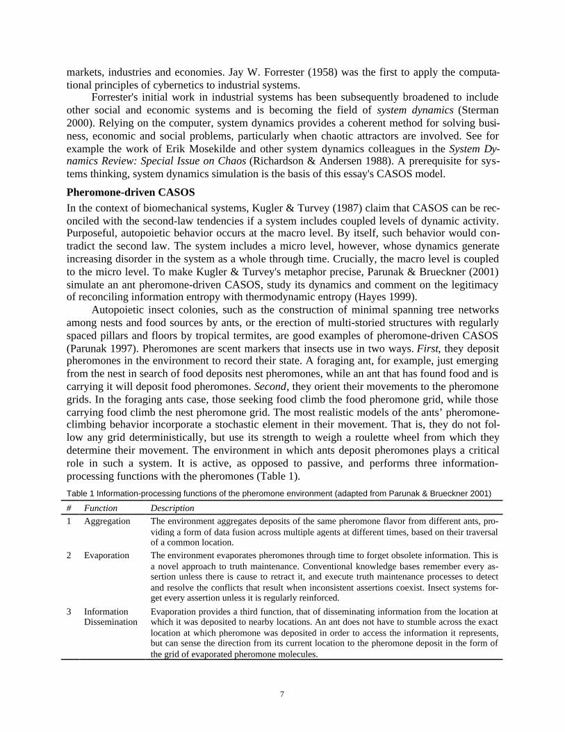
Autopoietic insect colonies, such as the construction of minimal spanning tree networksamong nests and food sources by ants, or the erection of multi-storied structures with regularlyspaced pillars and floors by tropical termites, are good examples of pheromone-driven CASOS(Parunak 1997). Pheromones are scent markers that insects use in two ways. First, they depositpheromones in the environment to record their state. A foraging ant, for example, just emergingfrom the nest in search of food deposits nest pheromones, while an ant that has found food and iscarrying it will deposit food pheromones. Second, they orient their movements to the pheromonegrids. In the foraging ants case, those seeking food climb the food pheromone grid, while thosecarrying food climb the nest pheromone grid. The most realistic models of the ants’ pheromone-climbing behavior incorporate a stochastic element in their movement. That is, they do not fol-low any grid deterministically, but use its strength to weigh a roulette wheel from which theydetermine their movement. The environment in which ants deposit pheromones plays a criticalrole in such a system. It is active, as opposed to passive, and performs three information-processing functions with the pheromones (Table 1).

Table 1 Information-processing functions of the pheromone environment (adapted from Parunak & Brueckner 2001)

# Function Description

1 Aggregation The environment aggregates deposits of the same pheromone flavor from different ants, pro-viding a form of data fusion across multiple agents at different times, based on their traversalof a common location.

2 Evaporation The environment evaporates pheromones through time to forget obsolete information. This isa novel approach to truth maintenance. Conventional knowledge bases remember every as-sertion unless there is cause to retract it, and execute truth maintenance processes to detectand resolve the conflicts that result when inconsistent assertions coexist. Insect systems for-get every assertion unless it is regularly reinforced.

3 InformationDissemination

Evaporation provides a third function, that of disseminating information from the location atwhich it was deposited to nearby locations. An ant does not have to stumble across the exactlocation at which pheromone was deposited in order to access the information it represents,but can sense the direction from its current location to the pheromone deposit in the form ofthe grid of evaporated pheromone molecules.

8

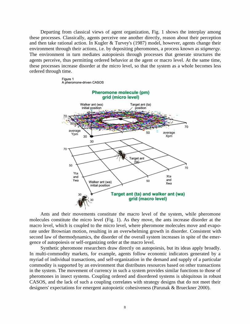
Departing from classical views of agent organization, Fig. 1 shows the interplay amongthese processes. Classically, agents perceive one another directly, reason about their perceptionand then take rational action. In Kugler & Turvey's (1987) model, however, agents change theirenvironment through their actions, i.e. by depositing pheromones, a process known as stigmergy.The environment in turn mediates autopoiesis through processes that generate structures theagents perceive, thus permitting ordered behavior at the agent or macro level. At the same time,these processes increase disorder at the micro level, so that the system as a whole becomes lessordered through time.

Ants and their movements constitute the macro level of the system, while pheromonemolecules constitute the micro level (Fig. 1). As they move, the ants increase disorder at themacro level, which is coupled to the micro level, where pheromone molecules move and evapo-rate under Brownian motion, resulting in an overwhelming growth in disorder. Consistent withsecond law of thermodynamics, the disorder of the overall system increases in spite of the emer-gence of autopoiesis or self-organizing order at the macro level.

Synthetic pheromone researchers draw directly on autopoiesis, but its ideas apply broadly.In multi-commodity markets, for example, agents follow economic indicators generated by amyriad of individual transactions, and self-organization in the demand and supply of a particularcommodity is supported by an environment that distributes resources based on other transactionsin the system. The movement of currency in such a system provides similar functions to those ofpheromones in insect systems. Coupling ordered and disordered systems is ubiquitous in robustCASOS, and the lack of such a coupling correlates with strategy designs that do not meet theirdesigners' expectations for emergent autopoietic cohesiveness (Parunak & Brueckner 2000).

9

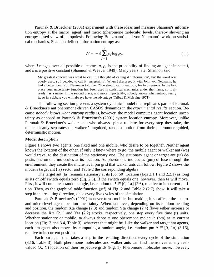
Parunak & Brueckner (2001) experiment with these ideas and measure Shannon's informa-tion entropy at the macro (agent) and micro (pheromone molecule) levels, thereby showing anentropy-based view of autopoiesis. Following Boltzmann's and von Neumann's work on statisti-cal mechanics, Shannon defined information entropy as:

where i ranges over all possible outcomes n, pi is the probability of finding an agent in state i,and k is a positive constant (Shannon & Weaver 1949). Many years later Shannon said:

My greatest concern was what to call it. I thought of calling it ‘information’, but the word wasoverly used, so I decided to call it ‘uncertainty’. When I discussed it with John von Neumann, hehad a better idea. Von Neumann told me: ‘You should call it entropy, for two reasons. In the firstplace your uncertainty function has been used in statistical mechanics under that name, so it al-ready has a name. In the second place, and more importantly, nobody knows what entropy reallyis, so in a debate you will always have the advantage (Tribus & McIrvine 1971).

The following section presents a system dynamics model that replicates parts of Parunak& Brueckner's ant pheromone-driven CASOS dynamics in the experimental results section. Be-cause nobody knows what entropy really is, however, the model computes agent location uncer-tainty as opposed to Parunak & Brueckner's (2001) system location entropy. Moreover, unlikeParunak & Brueckner's walker ants who always spin a roulette for every step they take, themodel cleanly separates the walkers' unguided, random motion from their pheromone-guided,deterministic motion.

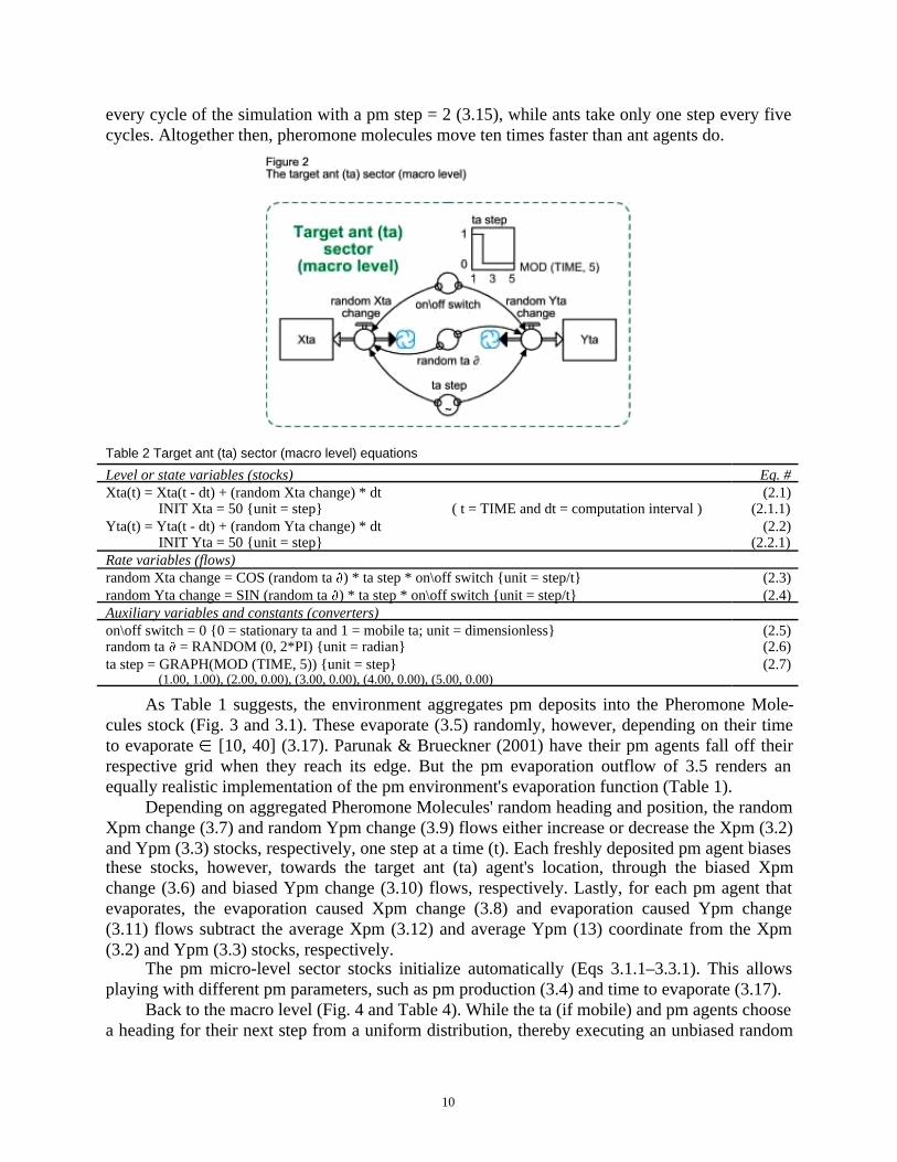
Model descriptionFigure 1 shows two agents, one fixed and one mobile, who desire to be together. Neither agentknows the location of the other. If only it knew where to go, the mobile agent or walker ant (wa)would travel to the destination of the stationary one. The stationary agent or target ant (ta) de-posits pheromone molecules at its location. As pheromone molecules (pm) diffuse through theenvironment, they create the micro-level pm grid that walker ants can follow. Figure 2 shows themodel's target ant (ta) sector and Table 2 the corresponding algebra.

The target ant (ta) remains stationary at its (50, 50) location (Eqs 2.1.1 and 2.2.1) as longas its on\off switch equals zero (Eq. 2.5). If the switch equals one, however, then ta will move.First, it will compute a random angle, i.e. random ta [0, 2 ] (2.6), relative to its current posi-tion. Then, as the graphical table function (gtf) of Fig. 2 and Table 2 (2.7) show, it will take astep in the resulting direction, once every five cycles of the simulation.

Parunak & Brueckner's (2001) ta never turns mobile, but making it so affects the macro-and micro-level agent location uncertainty. When ta moves, depending on its random headingand position, the random Xta change (2.3) and random Yta change (2.4) flows either increase ordecrease the Xta (2.1) and Yta (2.2) stocks, respectively, one step every five time (t) units.Whether stationary or mobile, ta always deposits one pheromone molecule (pm) at its currentlocation (Fig. 3 and 3.4, Table 3), whatever that might be. Like the walker and target ant agents,each pm agent also moves by computing a random angle, i.e. random pm [0, 2 ] (3.16),relative to its current position.

Each pm agent then takes a step in the resulting direction, every cycle of the simulation(3.16, Table 3). Both pheromone molecules and walker ants can find themselves at any real-valued (X, Y) location on their respective grids (Fig. 1). Pheromone molecules move, however,

10

every cycle of the simulation with a pm step = 2 (3.15), while ants take only one step every fivecycles. Altogether then, pheromone molecules move ten times faster than ant agents do.

Table 2 Target ant (ta) sector (macro level) equations

Level or state variables (stocks) Eq. #Xta(t) = Xta(t - dt) + (random Xta change) * dt

INIT Xta = 50 {unit = step} ( t = TIME and dt = computation interval )Yta(t) = Yta(t - dt) + (random Yta change) * dt

INIT Yta = 50 {unit = step}

(2.1)(2.1.1)

(2.2)(2.2.1)

Rate variables (flows)random Xta change = COS (random ta ) * ta step * on\off switch {unit = step/t}random Yta change = SIN (random ta ) * ta step * on\off switch {unit = step/t}

(2.3)(2.4)

Auxiliary variables and constants (converters)on\off switch = 0 {0 = stationary ta and 1 = mobile ta; unit = dimensionless}random ta = RANDOM (0, 2*PI) {unit = radian}ta step = GRAPH(MOD (TIME, 5)) {unit = step}

(1.00, 1.00), (2.00, 0.00), (3.00, 0.00), (4.00, 0.00), (5.00, 0.00)

(2.5)(2.6)(2.7)

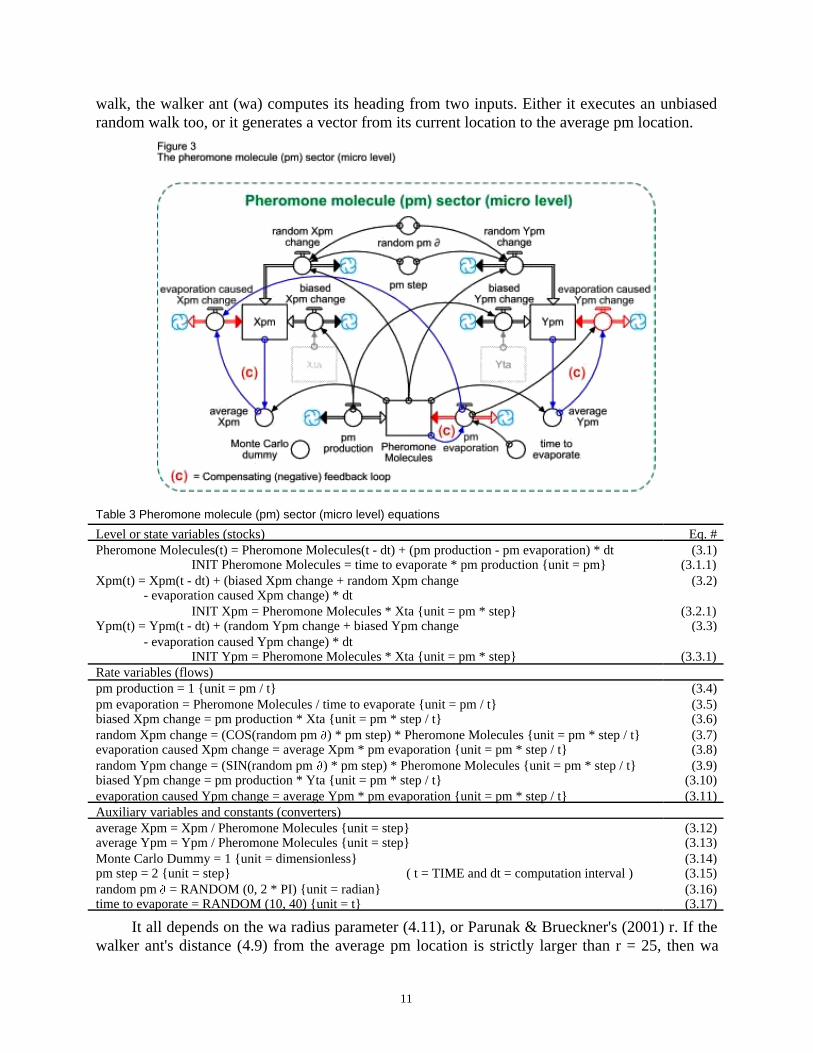
As Table 1 suggests, the environment aggregates pm deposits into the Pheromone Mole-cules stock (Fig. 3 and 3.1). These evaporate (3.5) randomly, however, depending on their timeto evaporate [10, 40] (3.17). Parunak & Brueckner (2001) have their pm agents fall off theirrespective grid when they reach its edge. But the pm evaporation outflow of 3.5 renders anequally realistic implementation of the pm environment's evaporation function (Table 1).

Depending on aggregated Pheromone Molecules' random heading and position, the randomXpm change (3.7) and random Ypm change (3.9) flows either increase or decrease the Xpm (3.2)and Ypm (3.3) stocks, respectively, one step at a time (t). Each freshly deposited pm agent biasesthese stocks, however, towards the target ant (ta) agent's location, through the biased Xpmchange (3.6) and biased Ypm change (3.10) flows, respectively. Lastly, for each pm agent thatevaporates, the evaporation caused Xpm change (3.8) and evaporation caused Ypm change(3.11) flows subtract the average Xpm (3.12) and average Ypm (13) coordinate from the Xpm(3.2) and Ypm (3.3) stocks, respectively.

The pm micro-level sector stocks initialize automatically (Eqs 3.1.1–3.3.1). This allowsplaying with different pm parameters, such as pm production (3.4) and time to evaporate (3.17).

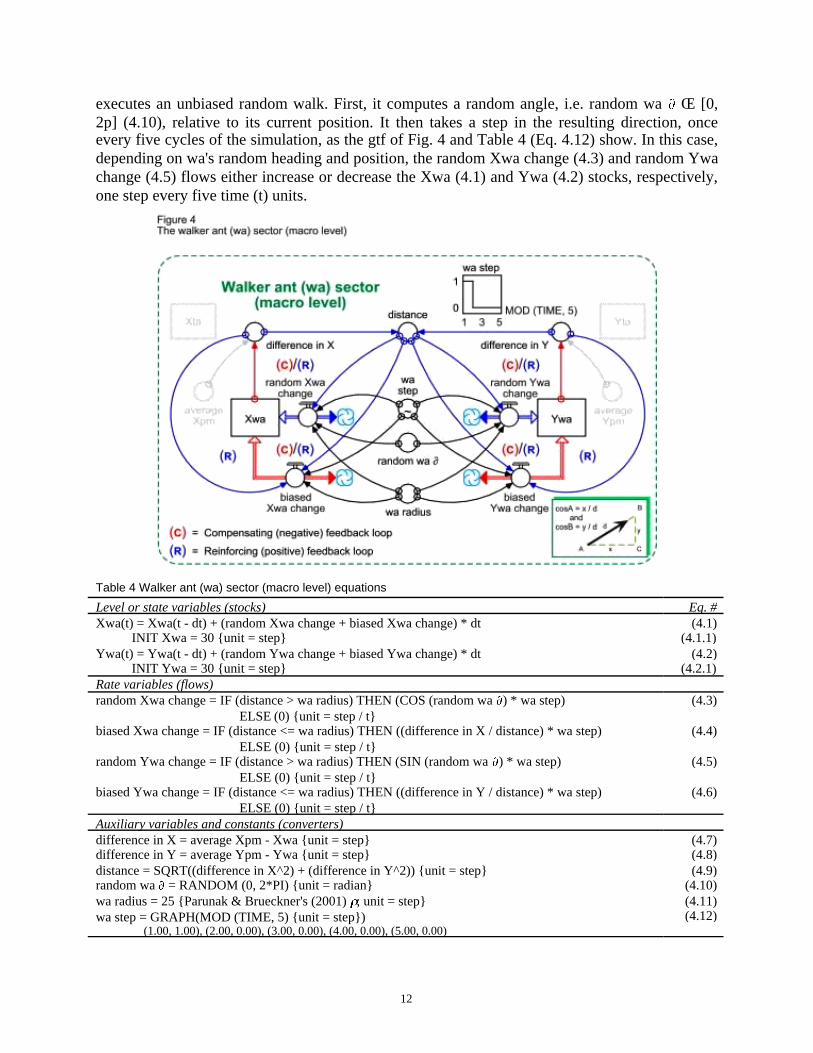
Back to the macro level (Fig. 4 and Table 4). While the ta (if mobile) and pm agents choosea heading for their next step from a uniform distribution, thereby executing an unbiased random

11

walk, the walker ant (wa) computes its heading from two inputs. Either it executes an unbiasedrandom walk too, or it generates a vector from its current location to the average pm location.

Table 3 Pheromone molecule (pm) sector (micro level) equations

Level or state variables (stocks) Eq. #Pheromone Molecules(t) = Pheromone Molecules(t - dt) + (pm production - pm evaporation) * dt

INIT Pheromone Molecules = time to evaporate * pm production {unit = pm}Xpm(t) = Xpm(t - dt) + (biased Xpm change + random Xpm change

- evaporation caused Xpm change) * dtINIT Xpm = Pheromone Molecules * Xta {unit = pm * step}

Ypm(t) = Ypm(t - dt) + (random Ypm change + biased Ypm change- evaporation caused Ypm change) * dt

INIT Ypm = Pheromone Molecules * Xta {unit = pm * step}

(3.1)(3.1.1)

(3.2)

(3.2.1)(3.3)

(3.3.1)Rate variables (flows)pm production = 1 {unit = pm / t}pm evaporation = Pheromone Molecules / time to evaporate {unit = pm / t}biased Xpm change = pm production * Xta {unit = pm * step / t}random Xpm change = (COS(random pm ) * pm step) * Pheromone Molecules {unit = pm * step / t}evaporation caused Xpm change = average Xpm * pm evaporation {unit = pm * step / t}random Ypm change = (SIN(random pm ) * pm step) * Pheromone Molecules {unit = pm * step / t}biased Ypm change = pm production * Yta {unit = pm * step / t}evaporation caused Ypm change = average Ypm * pm evaporation {unit = pm * step / t}

(3.4)(3.5)(3.6)(3.7)(3.8)(3.9)

(3.10)(3.11)

Auxiliary variables and constants (converters)average Xpm = Xpm / Pheromone Molecules {unit = step}average Ypm = Ypm / Pheromone Molecules {unit = step}Monte Carlo Dummy = 1 {unit = dimensionless}pm step = 2 {unit = step} ( t = TIME and dt = computation interval )random pm = RANDOM (0, 2 * PI) {unit = radian}time to evaporate = RANDOM (10, 40) {unit = t}

(3.12)(3.13)(3.14)(3.15)(3.16)(3.17)

It all depends on the wa radius parameter (4.11), or Parunak & Brueckner's (2001) r. If thewalker ant's distance (4.9) from the average pm location is strictly larger than r = 25, then wa

12

executes an unbiased random walk. First, it computes a random angle, i.e. random wa Π[0,2p] (4.10), relative to its current position. It then takes a step in the resulting direction, onceevery five cycles of the simulation, as the gtf of Fig. 4 and Table 4 (Eq. 4.12) show. In this case,depending on wa's random heading and position, the random Xwa change (4.3) and random Ywachange (4.5) flows either increase or decrease the Xwa (4.1) and Ywa (4.2) stocks, respectively,one step every five time (t) units.

Table 4 Walker ant (wa) sector (macro level) equations

Level or state variables (stocks) Eq. #Xwa(t) = Xwa(t - dt) + (random Xwa change + biased Xwa change) * dt

INIT Xwa = 30 {unit = step}Ywa(t) = Ywa(t - dt) + (random Ywa change + biased Ywa change) * dt

INIT Ywa = 30 {unit = step}

(4.1)(4.1.1)

(4.2)(4.2.1)

Rate variables (flows)random Xwa change = IF (distance > wa radius) THEN (COS (random wa ) * wa step)

ELSE (0) {unit = step / t}biased Xwa change = IF (distance <= wa radius) THEN ((difference in X / distance) * wa step)

ELSE (0) {unit = step / t}random Ywa change = IF (distance > wa radius) THEN (SIN (random wa ) * wa step)

ELSE (0) {unit = step / t}biased Ywa change = IF (distance <= wa radius) THEN ((difference in Y / distance) * wa step)

ELSE (0) {unit = step / t}

(4.3)

(4.4)

(4.5)

(4.6)

Auxiliary variables and constants (converters)difference in X = average Xpm - Xwa {unit = step}difference in Y = average Ypm - Ywa {unit = step}distance = SQRT((difference in X^2) + (difference in Y^2)) {unit = step}random wa = RANDOM (0, 2*PI) {unit = radian}wa radius = 25 {Parunak & Brueckner's (2001) ; unit = step}wa step = GRAPH(MOD (TIME, 5) {unit = step})

(1.00, 1.00), (2.00, 0.00), (3.00, 0.00), (4.00, 0.00), (5.00, 0.00)

(4.7)(4.8)(4.9)

(4.10)(4.11)(4.12)

13

If, however, wa's distance from the average pm location is less than or equal to = 25,then the walker ant climbs the pheromone molecule grid. That is, it computes a vector from itscurrent location to the average pm location. Depending on this vector's magnitude (see insert onlower right of Fig. 4), the biased Xwa change (4.4) and biased Ywa change (4.4) flows either in-crease or decrease the Xwa (4.1) and Ywa (4.2) stocks, respectively, every five time (t) units.

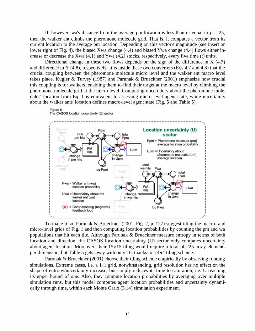
Directional change in these two flows depends on the sign of the difference in X (4.7)and difference in Y (4.8), respectively. It is inside these two converters (Eqs 4.7 and 4.8) that thecrucial coupling between the pheromone molecule micro level and the walker ant macro leveltakes place. Kugler & Turvey (1987) and Parunak & Brueckner (2001) emphasize how crucialthis coupling is for walkers, enabling them to find their target at the macro level by climbing thepheromone molecule grid at the micro level. Computing uncertainty about the pheromone mole-cules' location from Eq. 1 is equivalent to assessing micro-level agent state, while uncertaintyabout the walker ants' location defines macro-level agent state (Fig. 5 and Table 5).

To make it so, Parunak & Brueckner (2001, Fig. 2, p. 127) suggest tiling the macro- andmicro-level grids of Fig. 1 and then computing location probabilities by counting the pm and wapopulations that hit each tile. Although Parunak & Brueckner measure entropy in terms of bothlocation and direction, the CASOS location uncertainty (U) sector only computes uncertaintyabout agent location. Moreover, their 1515 tiling would require a total of 225 array elementsper dimension, but Table 5 gets away with only 16, thanks to a 44 tiling scheme.

Parunak & Brueckner (2001) choose their tiling scheme empirically by observing runningsimulations. Extreme cases, i.e. a 11 grid, notwithstanding, grid resolution has no effect on theshape of entropy/uncertainty increase, but simply reduces its time to saturation, i.e. U reachingits upper bound of one. Also, they compute location probabilities by averaging over multiplesimulation runs, but this model computes agent location probabilities and uncertainty dynami-cally through time, within each Monte Carlo (3.14) simulation experiment.

14

Table 5 Location uncertainty (U) sector equations

Level or state variables (stocks) Eq. #PM Hits[Tile # pm](t) = PM Hits[Tile # pm](t - dt) + (change in pm hits[Tile # pm]) * dt

INIT PM Hits[Tile # pm] = 0 {unit = hits}Upm(t) = Upm(t - dt) + (change in Upm) * dt

INIT Upm = 0Uwa(t) = Uwa(t - dt) + (change in Uwa) * dt

INIT Uwa = 0WA Hits[Tile # wa](t) = WA Hits[Tile # wa](t - dt) + (change in wa hits[Tile # wa]) * dt

INIT WA Hits[Tile # wa] = 0 {unit = hits}

(5.1)(5.1.1)

(5.2)(5.2.1)

(5.3)(5.3.1)

(5.4)(5.4.1)

Rate variables (flows)change in pm hits[1] = IF (10 <= average Xpm AND (average Xpm < 25) AND

(10 <= average Ypm) AND (average Ypm < 25)) THEN (1) Else (0) {unit = hits / t}

Mchange in pm hits[16] = IF (55 <= average Xpm AND (average Xpm < 70) AND

(55 <= average Ypm) AND (average Ypm < 70)) THEN (1) Else (0) {unit = hits / t}change in Upm = (total Ppm - Upm) * ( - ((Ppm[1] * log Ppm[1] + Ppm[2] * log Ppm[2] + Ppm[3] *

log Ppm[3] + Ppm[4] * log Ppm[4] + Ppm[5] * log Ppm[5] + Ppm[6] * log Ppm[6] + Ppm[7]* log Ppm[7] + Ppm[8] * log Ppm[8] + Ppm[9] * log Ppm[9] + Ppm[10] * log Ppm[10] +Ppm[11] * log Ppm[11] + Ppm[12] * log Ppm[12] + Ppm[13] * log Ppm[13] + Ppm[14] *log Ppm[14] + Ppm[15] * log Ppm[15] + Ppm[16] * log Ppm[16]) / LOG10(10)))

change in Uwa = (total Pwa - Uwa) * ( - ((Pwa[1] * log Pwa[1] + Pwa[2] * log Pwa[2] + Pwa[3] *log Pwa[3] + Pwa[4] * log Pwa[4] + Pwa[5] * log Pwa[5] + Pwa[6] * log Pwa[6] + Pwa[7] *log Pwa[7] + Pwa[8] * log Pwa[8] + Pwa[9] * log Pwa[9] + Pwa[10] * log Pwa[10] +Pwa[11] * log Pwa[11] + Pwa[12] * log Pwa[12] + Pwa[13] * log Pwa[13] + Pwa[14] *log Pwa[14] + Pwa[15] * log Pwa[15] + Pwa[16] * log Pwa[16]) / LOG10(10)))

change in wa hits[1] = IF (10 <= Xwa AND (Xwa < 25) AND (10 <= Ywa) AND (Ywa < 25))THEN (1) Else (0) {unit = hits / t}

Mchange in wa hits[16] = IF (55 <= Xwa AND (Xwa < 70) AND (55 <= Ywa) AND (Ywa < 70))

THEN (1) Else (0) {unit = hits / t}

(5.5)

(5. M )(5.20)

(5.21)

(5.22)

(5.23)

(5. M )(5.38)

Auxiliary variables and constants (converters)log Ppm[1] = IF (Ppm[1] = 0) THEN (0) ELSE (LOG10(Ppm[1]))

Mlog Ppm[16] = IF (Ppm[16] = 0) THEN (0) ELSE (LOG10(Ppm[16]))log Pwa[1] = IF (Pwa[1] = 0) THEN (0) ELSE (LOG10(Pwa[1]))

Mlog Pwa[16] = IF (Pwa[16] = 0) THEN (0) ELSE (LOG10(Pwa[16]))Ppm[1] = PM Hits[1] / total PM hits

MPpm[16] = PM Hits[16] / total PM hitsPwa[1] = WA Hits[1] / total WA hits

MPwa[16] = WA Hits[16] / total WA hitstotal pm hits = ARRAYSUM (PM Hits[*]) + 1 {unit = hits}total Ppm = ARRAYSUM(Ppm[*])total Pwa = ARRAYSUM(Pwa[*])total wa hits = ARRAYSUM (WA Hits[*]) + 1 {unit = hits}

(5.39)

(5. M )(5.54)(5.55)

(5. M )(5.70)(5.71)

(5. M )(5.86)(5.87)

(5. M )(5.102)(5.103)(5.104)(5.105)(5.106)

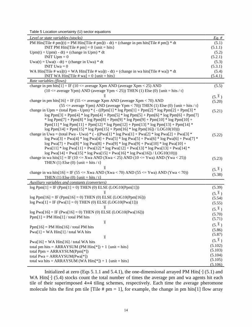
Initialized at zero (Eqs 5.1.1 and 5.4.1), the one-dimensional arrayed PM Hits[·] (5.1) andWA Hits[·] (5.4) stocks count the total number of times the average pm and wa agents hit eachtile of their superimposed 44 tiling schemes, respectively. Each time the average pheromonemolecule hits the first pm tile [Tile # pm = 1], for example, the change in pm hits[1] flow array

15

(5.5) adds a hit to the PM Hits[1] stock array (5.1). Similarly, each time a wa agent hits the 15thwalker ant tile [Tile # wa = 15], the change in wa hits[15] flow array (5.37) adds a hit to the WAHits[15] stock array (5.4).

Subsequently, the Ppm[1] converter array (5.71) computes the probability of the averagepm hitting the first pm tile [Tile # pm = 1] as the ratio of the PM Hits[1] stock array over the to-tal pm hits array sum (5.103). Similarly, the Pwa[15] converter array (5.101) computes the prob-ability of the wa hitting the 15th wa tile [Tile # wa = 15] as the ratio of the PM Hits[1] stock ar-ray over the total pm hits array sum (5.103). Adding a hit to these array sum converters (Eqs5.103 and 5.106) prevents their dividing by zero when all tiles are empty.

Once the arrayed Ppm[·] (Eqs 5.71–5.86) and Pwa[·] (Eqs 5.87-5.102) converters com-pute the micro- and macro-level agent location probabilities, respectively, the log Ppm[·] (Eqs5.39–5.54) and log Pwa[·] (Eqs 5.55-5.70) calculate their respective logarithms. Together, theprobabilities, their logarithms and the total probability array sums (5.104 and 5.105) affect thechange in Upm (5.21) and change in Uwa (5.22) flows that feed their respective pm and waagent location uncertainty stocks Upm (5.2) and Uwa (5.3). Each of the change in Upm (5.21)and change in Uwa (5.22) flows use Shannon's uncertainty formula (Eq. 1).

In the case of micro-level uncertainty about the pm average location (Upm), Shannon'spositive constant k gets smaller as Upm increases and its difference from the total pheromonemolecule average location probability (5.104) decreases. Similarly, in the case of macro-leveluncertainty about the walker ant location (Uwa), Shannon's positive constant k gets smaller asUwa increases and its difference from the total wa location probability (5.105) declines. In bothcases (5.21 and 5.22), following Parunak & Brueckner's (2001) suggestion, dividing the reportedagent location uncertainties by log(10) makes the logarithms' base irrelevant.

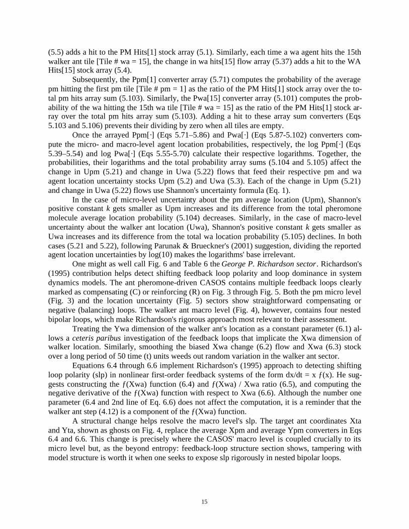
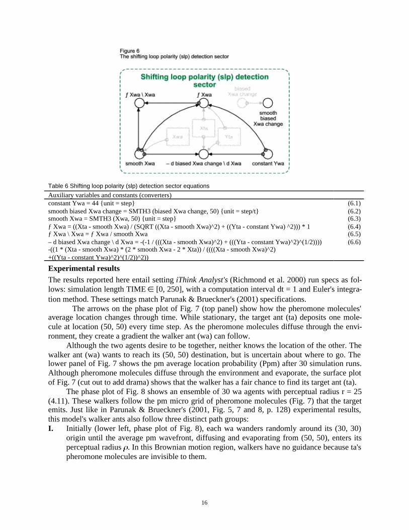
One might as well call Fig. 6 and Table 6 the George P. Richardson sector. Richardson's(1995) contribution helps detect shifting feedback loop polarity and loop dominance in systemdynamics models. The ant pheromone-driven CASOS contains multiple feedback loops clearlymarked as compensating (C) or reinforcing (R) on Fig. 3 through Fig. 5. Both the pm micro level(Fig. 3) and the location uncertainty (Fig. 5) sectors show straightforward compensating ornegative (balancing) loops. The walker ant macro level (Fig. 4), however, contains four nestedbipolar loops, which make Richardson's rigorous approach most relevant to their assessment.

Treating the Ywa dimension of the walker ant's location as a constant parameter (6.1) al-lows a ceteris paribus investigation of the feedback loops that implicate the Xwa dimension ofwalker location. Similarly, smoothing the biased Xwa change (6.2) flow and Xwa (6.3) stockover a long period of 50 time (t) units weeds out random variation in the walker ant sector.

Equations 6.4 through 6.6 implement Richardson's (1995) approach to detecting shiftingloop polarity (slp) in nonlinear first-order feedback systems of the form dx/dt = x ƒ(x). He sug-gests constructing the ƒ(Xwa) function (6.4) and ƒ(Xwa) / Xwa ratio (6.5), and computing thenegative derivative of the ƒ(Xwa) function with respect to Xwa (6.6). Although the number oneparameter (6.4 and 2nd line of Eq. 6.6) does not affect the computation, it is a reminder that thewalker ant step (4.12) is a component of the ƒ(Xwa) function.

A structural change helps resolve the macro level's slp. The target ant coordinates Xtaand Yta, shown as ghosts on Fig. 4, replace the average Xpm and average Ypm converters in Eqs6.4 and 6.6. This change is precisely where the CASOS' macro level is coupled crucially to itsmicro level but, as the beyond entropy: feedback-loop structure section shows, tampering withmodel structure is worth it when one seeks to expose slp rigorously in nested bipolar loops.

16

Table 6 Shifting loop polarity (slp) detection sector equations

Auxiliary variables and constants (converters)constant Ywa = 44 {unit = step}smooth biased Xwa change = SMTH3 (biased Xwa change, 50) {unit = step/t}smooth Xwa = SMTH3 (Xwa, 50) {unit = step}ƒ Xwa = ((Xta - smooth Xwa) / (SQRT ((Xta - smooth Xwa)^2) + ((Yta - constant Ywa) ^2))) * 1ƒ Xwa \ Xwa = ƒ Xwa / smooth Xwa– d biased Xwa change \ d Xwa = -(-1 / (((Xta - smooth Xwa)^2) + (((Yta - constant Ywa)^2)^(1/2))))-((1 * (Xta - smooth Xwa) * (2 * smooth Xwa - 2 * Xta)) / ((((Xta - smooth Xwa)^2)+((Yta - constant Ywa)^2)^(1/2))^2))

(6.1)(6.2)(6.3)(6.4)(6.5)(6.6)

Experimental resultsThe results reported here entail setting iThink Analyst's (Richmond et al. 2000) run specs as fol-lows: simulation length TIME [0, 250], with a computation interval dt = 1 and Euler's integra-tion method. These settings match Parunak & Brueckner's (2001) specifications.

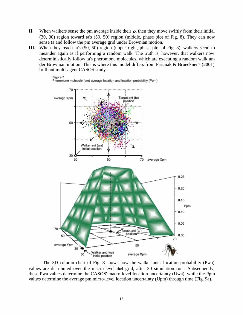
The arrows on the phase plot of Fig. 7 (top panel) show how the pheromone molecules'average location changes through time. While stationary, the target ant (ta) deposits one mole-cule at location (50, 50) every time step. As the pheromone molecules diffuse through the envi-ronment, they create a gradient the walker ant (wa) can follow.

Although the two agents desire to be together, neither knows the location of the other. Thewalker ant (wa) wants to reach its (50, 50) destination, but is uncertain about where to go. Thelower panel of Fig. 7 shows the pm average location probability (Ppm) after 30 simulation runs.Although pheromone molecules diffuse through the environment and evaporate, the surface plotof Fig. 7 (cut out to add drama) shows that the walker has a fair chance to find its target ant (ta).

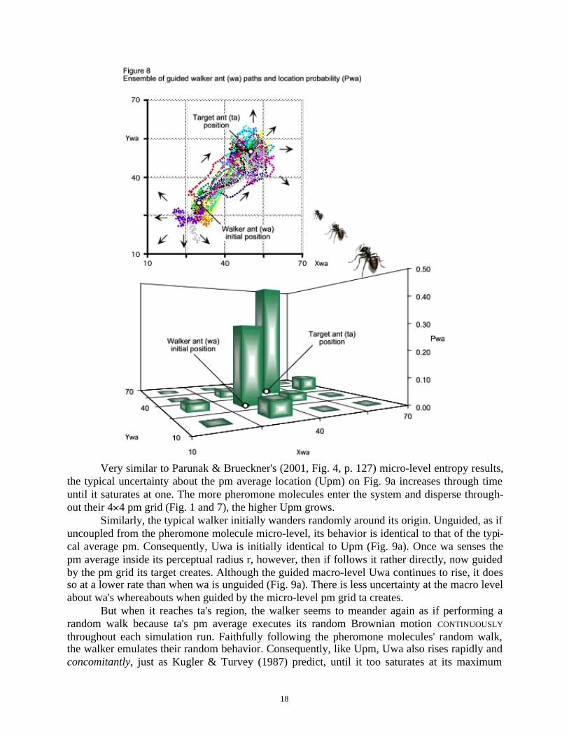
The phase plot of Fig. 8 shows an ensemble of 30 wa agents with perceptual radius r = 25(4.11). These walkers follow the pm micro grid of pheromone molecules (Fig. 7) that the targetemits. Just like in Parunak & Brueckner's (2001, Fig. 5, 7 and 8, p. 128) experimental results,this model's walker ants also follow three distinct path groups:I. Initially (lower left, phase plot of Fig. 8), each wa wanders randomly around its (30, 30)

origin until the average pm wavefront, diffusing and evaporating from (50, 50), enters itsperceptual radius . In this Brownian motion region, walkers have no guidance because ta'spheromone molecules are invisible to them.

17

II. When walkers sense the pm average inside their , then they move swiftly from their initial(30, 30) region toward ta's (50, 50) region (middle, phase plot of Fig. 8). They can nowsense ta and follow the pm average grid under Brownian motion.

III. When they reach ta's (50, 50) region (upper right, phase plot of Fig. 8), walkers seem tomeander again as if performing a random walk. The truth is, however, that walkers nowdeterministically follow ta's pheromone molecules, which are executing a random walk un-der Brownian motion. This is where this model differs from Parunak & Brueckner's (2001)brilliant multi-agent CASOS study.

The 3D column chart of Fig. 8 shows how the walker ants' location probability (Pwa)values are distributed over the macro-level 44 grid, after 30 simulation runs. Subsequently,these Pwa values determine the CASOS' macro-level location uncertainty (Uwa), while the Ppmvalues determine the average pm micro-level location uncertainty (Upm) through time (Fig. 9a).

18

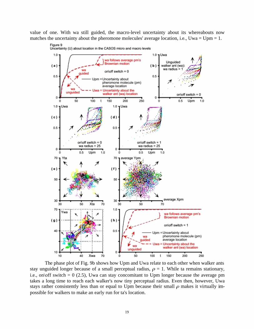
Very similar to Parunak & Brueckner's (2001, Fig. 4, p. 127) micro-level entropy results,the typical uncertainty about the pm average location (Upm) on Fig. 9a increases through timeuntil it saturates at one. The more pheromone molecules enter the system and disperse through-out their 4 4 pm grid (Fig. 1 and 7), the higher Upm grows.

Similarly, the typical walker initially wanders randomly around its origin. Unguided, as ifuncoupled from the pheromone molecule micro-level, its behavior is identical to that of the typi-cal average pm. Consequently, Uwa is initially identical to Upm (Fig. 9a). Once wa senses thepm average inside its perceptual radius r, however, then if follows it rather directly, now guidedby the pm grid its target creates. Although the guided macro-level Uwa continues to rise, it doesso at a lower rate than when wa is unguided (Fig. 9a). There is less uncertainty at the macro levelabout wa's whereabouts when guided by the micro-level pm grid ta creates.

But when it reaches ta's region, the walker seems to meander again as if performing arandom walk because ta's pm average executes its random Brownian motion CONTINUOUSLY

throughout each simulation run. Faithfully following the pheromone molecules' random walk,the walker emulates their random behavior. Consequently, like Upm, Uwa also rises rapidly andconcomitantly, just as Kugler & Turvey (1987) predict, until it too saturates at its maximum

19

value of one. With wa still guided, the macro-level uncertainty about its whereabouts nowmatches the uncertainty about the pheromone molecules' average location, i.e., Uwa = Upm = 1.

The phase plot of Fig. 9b shows how Upm and Uwa relate to each other when walker antsstay unguided longer because of a small perceptual radius, = 1. While ta remains stationary,i.e., on\off switch = 0 (2.5), Uwa can stay concomitant to Upm longer because the average pmtakes a long time to reach each walker's now tiny perceptual radius. Even then, however, Uwastays rather consistently less than or equal to Upm because their small makes it virtually im-possible for walkers to make an early run for ta's location.

20

With reset to 25 (Fig. 9c), some walkers sometimes perceive their target early, beforepheromone molecules have a chance to diffuse far enough from ta's initial location. When thathappens, the average pm location guides walkers early and Uwa exceeds Upm for a while.Eventually, however, whether early or late, walkers always fall pray to the average pheromone'sBrownian motion and the inevitable happens: Uwa = Upm = 1. Both the macro and the microCASOS levels become equally uncertain about their respective agents' location. Interestinglyenough, when the stationary ta turns mobile, i.e. on\off switch = 1, then Uwa exceeds Upm less(Fig. 9d). Doubling randomness at the micro level causes Upm to seclude Uwa more frequently,thereby sequestering the agent location uncertainty Uwa at the macro level.

As target ants now meander continuously under their newly acquired mobility (Fig. 9e),they cause the pheromone molecules they emit to diffuse more vigorously through the environ-ment (compare Fig. 9f to the phase plot of Fig. 7). Because of their initial random walk aroundtheir origin, walkers in different runs again will be at different locations when they start to sensea ta and will follow slightly different paths to their target (Fig. 9g). The excess pm randomness atthe micro level, however, while still sequestering uncertainty/entropy at the macro level, it doesso for a shorter time. It shortens both the time a typical wa stays unguided and the time it takes awalker to move to the now enlarged ta region (Fig. 9h; compare to Fig. 9a).

In addition to confirming Kugler & Turvey's (1987) concomitant entropy prediction aswell as some of Parunak & Brueckner's (2201) dynamics, these results are consistent with theself-organization seen in cybernetics, dissipative structures and thermodynamic fluctuations,where the larger their randomness, the faster systems become autopoietic, i.e., produce order.While Upm sequesters Uwa in most cases, the larger the uncertainty about the pheromone mole-cules' average location at the micro level, the faster the macro system self-organizes, i.e. thefaster walkers move from their initial region to their now mobile target's region. Doubling ran-domness at the micro level pushes the system as a whole faster to its stable point attractor, whereUwa = Upm = 1.

Where these results differ, however, from Parunak & Brueckner's (2001, Fig. 6, p. 128),is in the unguided walker entropy (here Uwa). How is it possible for the unguided walker, whenit acts just like a pm, executing a random walk, to produce entropy so vastly different from thepheromones'? The vast discrepancy between their Fig. 4 (p. 127) and Fig. 6 (p. 128) makes onewander about their method. This essay's Fig. 9 shows that, even under different experimentalconditions, Upm and Uwa are identical as long as the pheromone molecules at the micro leveland the unguided walker ants at the macro level are executing random walks. Moreover, whiletrying to assess entropy in the overall CASOS, Parunak & Brueckner finally ask whether se-questering "macro (walker) entropy is causally related to the increase in micro entropy, or justcoincidental" (2001, p. 129). Even if rhetorical, this question begs for a system dynamics demon-stration. How well can system dynamics explain causal relations in circular feedback loops thatproduce nonlinear dynamics spontaneously out of their local interactions? Let's see.

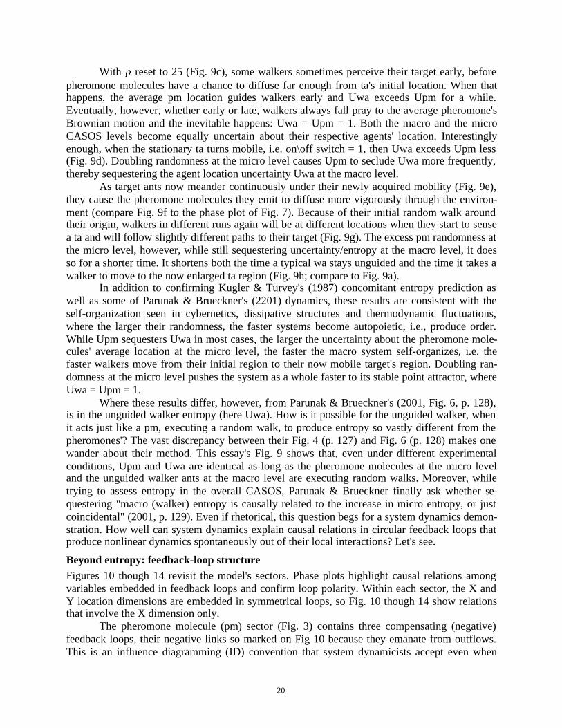
Beyond entropy: feedback-loop structureFigures 10 though 14 revisit the model's sectors. Phase plots highlight causal relations amongvariables embedded in feedback loops and confirm loop polarity. Within each sector, the X andY location dimensions are embedded in symmetrical loops, so Fig. 10 though 14 show relationsthat involve the X dimension only.

The pheromone molecule (pm) sector (Fig. 3) contains three compensating (negative)feedback loops, their negative links so marked on Fig 10 because they emanate from outflows.This is an influence diagramming (ID) convention that system dynamicists accept even when

21

they define loop polarity rigorously (Richardson 1995). But these loops' real polarity depends ontime to evaporate (3.17), a random parameter whose sign is set by environmental conditions out-side the loops. Although the nonlinear negative relation between time to evaporate (3.17) and thepm evaporation (3.5) outflow (Fig. 10a) plays outside these loops, it does turn them positive.Then, they drive the pm average so far that walkers never sense their targets. Or, alternatively,they bring it inside the wa's perceptual radius so fast that uncertainty about walker location at themacro level (Uwa) exceeds Upm at the micro level (Fig. 9c and d).

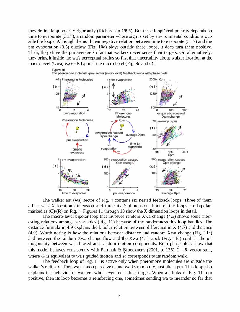
The walker ant (wa) sector of Fig. 4 contains six nested feedback loops. Three of themaffect wa's X location dimension and three its Y dimension. Four of the loops are bipolar,marked as (C)/(R) on Fig. 4. Figures 11 through 13 show the X dimension loops in detail.

The macro-level bipolar loop that involves random Xwa change (4.3) shows some inter-esting relations among its variables (Fig. 11) because of the randomness this loop handles. Thedistance formula in 4.9 explains the bipolar relation between difference in X (4.7) and distance(4.9). Worth noting is how the relations between distance and random Xwa change (Fig. 11c)and between the random Xwa change flow and the Xwa (4.1) stock (Fig. 11d) confirm the or-thogonality between wa's biased and random motion components. Both phase plots show thatthis model behaves consistently with Parunak & Brueckner's (2001, p. 126)

r G

r R vector sum,

where r G is equivalent to wa's guided motion and

r R corresponds to its random walk.

The feedback loop of Fig. 11 is active only when pheromone molecules are outside thewalker's radius . Then wa cannon perceive ta and walks randomly, just like a pm. This loop alsoexplains the behavior of walkers who never meet their target. When all links of Fig. 11 turnpositive, then its loop becomes a reinforcing one, sometimes sending wa to meander so far that

22

the pm average cannot ever enter its perceptual radius. Oddly enough, the same loop can alsoexplain the behavior of walkers who go meet their target so fast that uncertainty about walkerlocation at the macro level (Uwa) exceeds Upm at the micro level (Fig. 9c and d).

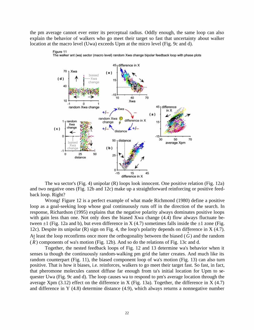
The wa sector's (Fig. 4) unipolar (R) loops look innocent. One positive relation (Fig. 12a)and two negative ones (Fig. 12b and 12c) make up a straightforward reinforcing or positive feed-back loop. Right?

Wrong! Figure 12 is a perfect example of what made Richmond (1980) define a positiveloop as a goal-seeking loop whose goal continuously runs off in the direction of the search. Inresponse, Richardson (1995) explains that the negative polarity always dominates positive loopswith gain less than one. Not only does the biased Xwa change (4.4) flow always fluctuate be-tween ±1 (Fig. 12a and b), but even difference in X (4.7) sometimes falls inside the ±1 zone (Fig.12c). Despite its unipolar (R) sign on Fig. 4, the loop's polarity depends on difference in X (4.7).At least the loop reconfirms once more the orthogonality between the biased (

r G ) and the random

( r R ) components of wa's motion (Fig. 12b). And so do the relations of Fig. 13c and d.

Together, the nested feedback loops of Fig. 12 and 13 determine wa's behavior when itsenses ta though the continuously random-walking pm grid the latter creates. And much like itsrandom counterpart (Fig. 11), the biased component loop of wa's motion (Fig. 13) can also turnpositive. That is how it biases, i.e. reinforces, walkers to go meet their target fast. So fast, in fact,that pheromone molecules cannot diffuse far enough from ta's initial location for Upm to se-quester Uwa (Fig. 9c and d). The loop causes wa to respond to pm's average location through theaverage Xpm (3.12) effect on the difference in X (Fig. 13a). Together, the difference in X (4.7)and difference in Y (4.8) determine distance (4.9), which always returns a nonnegative number

23

(Fig. 13b). The net effect of distance on Xwa (4.1) is negative relation (Fig. 13e) and, closing thecircle, Xwa (4.1) has a negative effect on the difference in X (Fig. 13f).

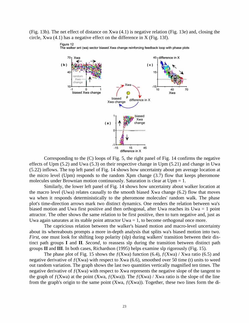
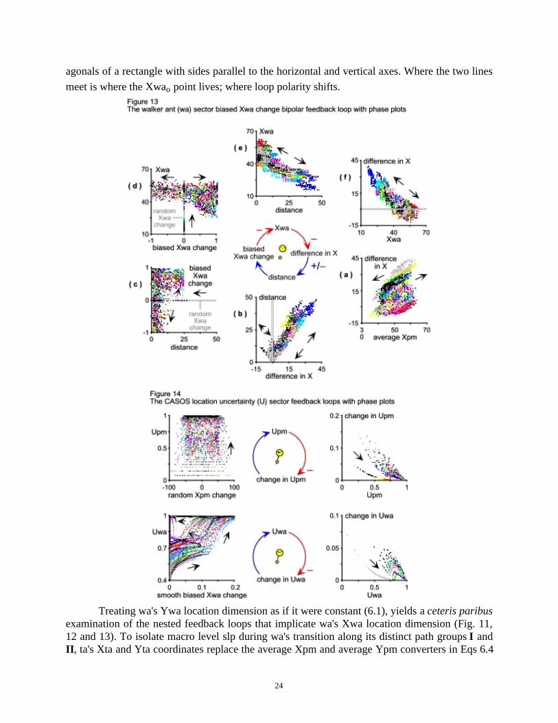
Corresponding to the (C) loops of Fig. 5, the right panel of Fig. 14 confirms the negativeeffects of Upm (5.2) and Uwa (5.3) on their respective change in Upm (5.21) and change in Uwa(5.22) inflows. The top left panel of Fig. 14 shows how uncertainty about pm average location atthe micro level (Upm) responds to the random Xpm change (3.7) flow that keeps pheromonemolecules under Brownian motion continuously. Saturation is clear at Upm = 1.

Similarly, the lower left panel of Fig. 14 shows how uncertainty about walker location atthe macro level (Uwa) relates causally to the smooth biased Xwa change (6.2) flow that moveswa when it responds deterministically to the pheromone molecules' random walk. The phaseplot's time-direction arrows mark two distinct dynamics. One renders the relation between wa'sbiased motion and Uwa first positive and then orthogonal, after Uwa reaches its Uwa = 1 pointattractor. The other shows the same relation to be first positive, then to turn negative and, just asUwa again saturates at its stable point attractor Uwa = 1, to become orthogonal once more.

The capricious relation between the walker's biased motion and macro-level uncertaintyabout its whereabouts prompts a more in-depth analysis that splits wa's biased motion into two.First, one must look for shifting loop polarity (slp) during walkers' transition between their dis-tinct path groups I and II . Second, to reassess slp during the transition between distinct pathgroups II and III . In both cases, Richardson (1995) helps examine slp rigorously (Fig. 15).

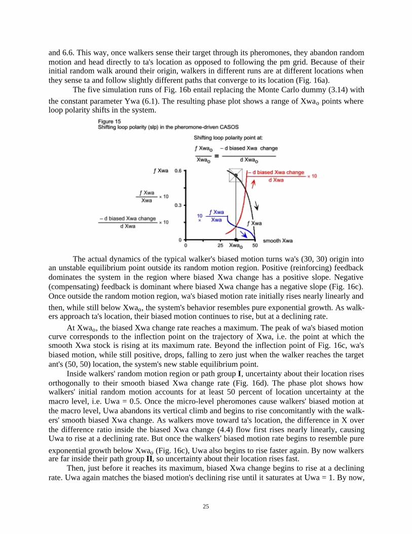
The phase plot of Fig. 15 shows the ƒ(Xwa) function (6.4), ƒ(Xwa) / Xwa ratio (6.5) andnegative derivative of ƒ(Xwa) with respect to Xwa (6.6), smoothed over 50 time (t) units to weedout random variation. The graph shows the last two quantities vertically magnified ten times. Thenegative derivative of ƒ(Xwa) with respect to Xwa represents the negative slope of the tangent tothe graph of ƒ(Xwa) at the point (Xwa, ƒ(Xwa)). The ƒ(Xwa) / Xwa ratio is the slope of the linefrom the graph's origin to the same point (Xwa, ƒ(Xwa)). Together, these two lines form the di-

24

agonals of a rectangle with sides parallel to the horizontal and vertical axes. Where the two lines

meet is where the Xwao point lives; where loop polarity shifts.

Treating wa's Ywa location dimension as if it were constant (6.1), yields a ceteris paribusexamination of the nested feedback loops that implicate wa's Xwa location dimension (Fig. 11,12 and 13). To isolate macro level slp during wa's transition along its distinct path groups I andII , ta's Xta and Yta coordinates replace the average Xpm and average Ypm converters in Eqs 6.4

25

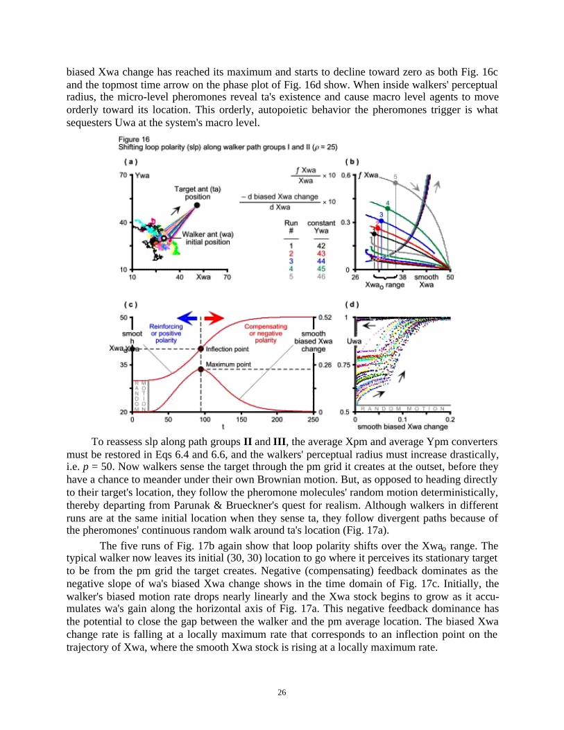
and 6.6. This way, once walkers sense their target through its pheromones, they abandon randommotion and head directly to ta's location as opposed to following the pm grid. Because of theirinitial random walk around their origin, walkers in different runs are at different locations whenthey sense ta and follow slightly different paths that converge to its location (Fig. 16a).

The five simulation runs of Fig. 16b entail replacing the Monte Carlo dummy (3.14) with

the constant parameter Ywa (6.1). The resulting phase plot shows a range of Xwao points whereloop polarity shifts in the system.

The actual dynamics of the typical walker's biased motion turns wa's (30, 30) origin intoan unstable equilibrium point outside its random motion region. Positive (reinforcing) feedbackdominates the system in the region where biased Xwa change has a positive slope. Negative(compensating) feedback is dominant where biased Xwa change has a negative slope (Fig. 16c).Once outside the random motion region, wa's biased motion rate initially rises nearly linearly and

then, while still below Xwao, the system's behavior resembles pure exponential growth. As walk-ers approach ta's location, their biased motion continues to rise, but at a declining rate.

At Xwao, the biased Xwa change rate reaches a maximum. The peak of wa's biased motioncurve corresponds to the inflection point on the trajectory of Xwa, i.e. the point at which thesmooth Xwa stock is rising at its maximum rate. Beyond the inflection point of Fig. 16c, wa'sbiased motion, while still positive, drops, falling to zero just when the walker reaches the targetant's (50, 50) location, the system's new stable equilibrium point.

Inside walkers' random motion region or path group I , uncertainty about their location risesorthogonally to their smooth biased Xwa change rate (Fig. 16d). The phase plot shows howwalkers' initial random motion accounts for at least 50 percent of location uncertainty at themacro level, i.e. Uwa = 0.5. Once the micro-level pheromones cause walkers' biased motion atthe macro level, Uwa abandons its vertical climb and begins to rise concomitantly with the walk-ers' smooth biased Xwa change. As walkers move toward ta's location, the difference in X overthe difference ratio inside the biased Xwa change (4.4) flow first rises nearly linearly, causingUwa to rise at a declining rate. But once the walkers' biased motion rate begins to resemble pure

exponential growth below Xwao (Fig. 16c), Uwa also begins to rise faster again. By now walkersare far inside their path group II , so uncertainty about their location rises fast.

Then, just before it reaches its maximum, biased Xwa change begins to rise at a decliningrate. Uwa again matches the biased motion's declining rise until it saturates at Uwa = 1. By now,

26

biased Xwa change has reached its maximum and starts to decline toward zero as both Fig. 16cand the topmost time arrow on the phase plot of Fig. 16d show. When inside walkers' perceptualradius, the micro-level pheromones reveal ta's existence and cause macro level agents to moveorderly toward its location. This orderly, autopoietic behavior the pheromones trigger is whatsequesters Uwa at the system's macro level.

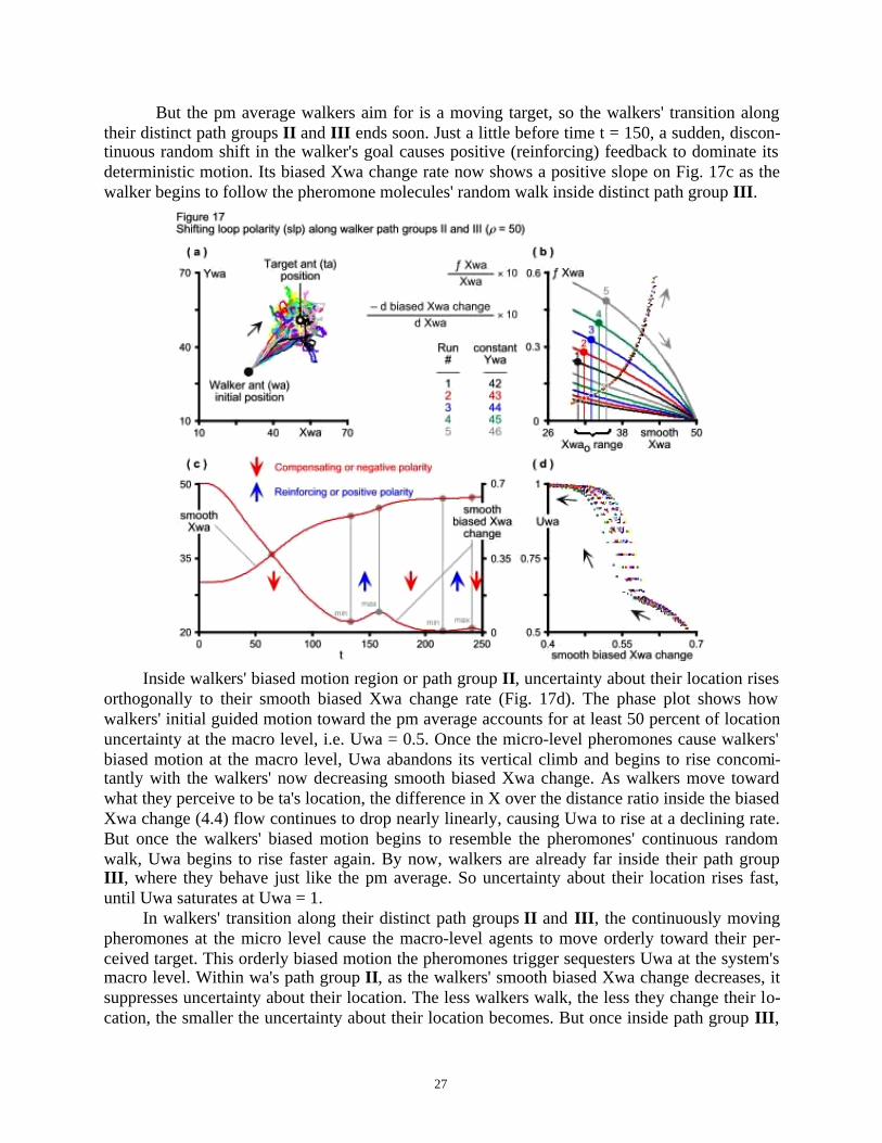
To reassess slp along path groups II and III , the average Xpm and average Ypm convertersmust be restored in Eqs 6.4 and 6.6, and the walkers' perceptual radius must increase drastically,i.e. p = 50. Now walkers sense the target through the pm grid it creates at the outset, before theyhave a chance to meander under their own Brownian motion. But, as opposed to heading directlyto their target's location, they follow the pheromone molecules' random motion deterministically,thereby departing from Parunak & Brueckner's quest for realism. Although walkers in differentruns are at the same initial location when they sense ta, they follow divergent paths because ofthe pheromones' continuous random walk around ta's location (Fig. 17a).

The five runs of Fig. 17b again show that loop polarity shifts over the Xwao range. Thetypical walker now leaves its initial (30, 30) location to go where it perceives its stationary targetto be from the pm grid the target creates. Negative (compensating) feedback dominates as thenegative slope of wa's biased Xwa change shows in the time domain of Fig. 17c. Initially, thewalker's biased motion rate drops nearly linearly and the Xwa stock begins to grow as it accu-mulates wa's gain along the horizontal axis of Fig. 17a. This negative feedback dominance hasthe potential to close the gap between the walker and the pm average location. The biased Xwachange rate is falling at a locally maximum rate that corresponds to an inflection point on thetrajectory of Xwa, where the smooth Xwa stock is rising at a locally maximum rate.

27

But the pm average walkers aim for is a moving target, so the walkers' transition alongtheir distinct path groups II and III ends soon. Just a little before time t = 150, a sudden, discon-tinuous random shift in the walker's goal causes positive (reinforcing) feedback to dominate itsdeterministic motion. Its biased Xwa change rate now shows a positive slope on Fig. 17c as thewalker begins to follow the pheromone molecules' random walk inside distinct path group III .

Inside walkers' biased motion region or path group II , uncertainty about their location risesorthogonally to their smooth biased Xwa change rate (Fig. 17d). The phase plot shows howwalkers' initial guided motion toward the pm average accounts for at least 50 percent of locationuncertainty at the macro level, i.e. Uwa = 0.5. Once the micro-level pheromones cause walkers'biased motion at the macro level, Uwa abandons its vertical climb and begins to rise concomi-tantly with the walkers' now decreasing smooth biased Xwa change. As walkers move towardwhat they perceive to be ta's location, the difference in X over the distance ratio inside the biasedXwa change (4.4) flow continues to drop nearly linearly, causing Uwa to rise at a declining rate.But once the walkers' biased motion begins to resemble the pheromones' continuous randomwalk, Uwa begins to rise faster again. By now, walkers are already far inside their path groupIII , where they behave just like the pm average. So uncertainty about their location rises fast,until Uwa saturates at Uwa = 1.

In walkers' transition along their distinct path groups II and III , the continuously movingpheromones at the micro level cause the macro-level agents to move orderly toward their per-ceived target. This orderly biased motion the pheromones trigger sequesters Uwa at the system'smacro level. Within wa's path group II , as the walkers' smooth biased Xwa change decreases, itsuppresses uncertainty about their location. The less walkers walk, the less they change their lo-cation, the smaller the uncertainty about their location becomes. But once inside path group III ,

28

walkers fall pray to the pheromones' random motion, following them around deterministically.Uncertainty about their location now rises fast at the macro level, eventually matching uncer-tainty about pm average location at the micro level, i.e. Uwa = Upm = 1.

When inside walkers' perceptual radius, the micro-level pheromones reveal the targetagent's existence and cause macro level agents to move orderly toward its location. This orderly,autopoietic behavior the pheromones trigger is what sequesters Uwa at the system's macro level.

ConclusionAlong with Prophet Sulayman's armies, the Qur'an mentions the ants' advanced communicationssystem (Yahya, 2000). Here is the verse:

Then, when they reached the valley of the ants, an ant said: 'Ants! Enter your dwellings so thatSulayman and his troops do not crush you unwittingly' (Surat an-Naml: 18).

Scientific research confirms the incredible communications network among these creatures. Us-ing system dynamics to play with the ants and to understand complex, adaptive, self-organizingsystems means looking at autopoietic processes causally, as opposed to merely at entropy meas-ures. This model also replicated parts of Parunak & Brueckner's (2001) results. Despite its pre-sent inability to tag undifferentiated agents' attributes (Scholl 2001), the system dynamicsmethod and software helps to understand exactly how CASOS' circular or feedback-loop rela-tions produce nonlinear dynamics spontaneously out of their local interactions. As shifting looppolarity (slp) determines system behavior (Richardson 1995), distributed control leads positivefeedback relations to explosive growth, which ends when all dynamics has been absorbed into anattractor, leaving the system in a stable, negative feedback state.

In addition to replicating parts of Parunak & Brueckner's (2001) results, the model recon-firms that the larger the random perturbations (noise) that affect a system, the more quickly itwill self-organize to produce order. Replacing the if-then-else statements of Table 4 with agraphical table function (gtf) does not change the dynamics much, but does increase the numberof loops in the wa sector from six to eight. Another variant entails letting walkers random-walkcontinuously, just like the pheromones do, even while these walkers chase pheromones. That re-duces the wa sector loops from six to four and brings the model closer to what Parunak &Brueckner (2001, p. 125) see as "most realistic" behavior in their multi-agent CASOS study. Butthen it becomes impossible to separate the walkers' randomness from the pheromones'.

Assessing slp separately in walkers' transition, first between their distinct path groups Iand II , and then again between groups II and III , helps explain the dynamics of the relation be-tween walkers' biased motion rate and the macro-level uncertainty Uwa (lower left panel of Fig.14). When walkers abandon their random walk to go meet their target, then the relation betweentheir biased motion and Uwa becomes positive (Fig. 16d). However, when they deterministicallyfollow the Brownian motion of the pheromones their target emits, then the same relation turnsnegative (Fig. 17d). In the first case, the walkers change their location under reinforcing or posi-tive feedback (Fig. 16c). In the second case, they change their location under compensating ornegative feedback (Fig. 17c). In both cases, Uwa rises because the walkers' location changes.

It is interesting to see, however, that as agents move from random disorder to autopoieticorder with deterministic rules (Fig. 16a), then it is positive feedback that causes the relation be-tween their rate of motion and location uncertainty to become positive (Fig. 16d). Conversely,when agents move, again deterministically, from static order to random disorder, then it is nega-tive feedback that causes the relation between their rate of motion and location uncertainty tobecome negative (Fig. 17d).

29

In business, Williams (2002) sees a trend toward more customer intimacy in systems forpersonalization and communities of interest. This trend does not necessarily imply emergence,but one example of it, eBay, is an excellent business example of emergent behavior creatingCASOS communities of interest. Another example is Bussmann & Schild's (2000) auction-based, self-organizing manufacturing control. DaimlerChrysler is evaluating this approach as abypass to its existing manufacturing line. Performance tests demonstrate the industrial feasibilityand benefits of self organization. And let's not forget the Star Trek-inspired Intelligent Room(Hanssens et al. 2002), which is changing what it means to use a computer. Rather than view acomputer as a stand-alone box good only for word processing or e-mail, MIT's Intelligent Roomis embedding computers in ordinary environments so that people can interact with them the waythey do with other people, by speech, gesture, movement, affect and context.

In the context of practical CASOS action, Rough (1997) argues that CASOS facilitatorsmust elicit and sustain breakthrough change processes, whether in persons, groups or organiza-tions. Rather than trying to explain or to order what is needed, the facilitator attends to thechange process and trusts that things will self-organize. The mechanistic paradigm we live inmakes CASOS changes seem like magic. To understand CASOS facilitation, one must recognizethe difference between managed change and self-organizing change. Rough's (1997) CASOSapplication examples include: (a) new insights where problems are spontaneously solved, (b)changes of heart where the trust level shifts and adversaries become friends, (c) a shift from de-pendency to empowerment, (d) a change of management style, from control to self-managementand (e) people discovering what they really want instead of what they thought they wanted.

CASOS metaphors are good as far as they provide a springboard for discussion about thepossibilities that emerge when combining physical and social sciences. To benefit from them,however, business managers and researchers must preserve CASOS rigor. System dynamicshelps to explain why and to see exactly how CASOS generate their magnificent patterns; howCASOS structure causes autopoietic behavior. System dynamics perhaps can help articulate aninterdisciplinary, posthumanist CASOS theory that shifts between contradictory elements in oldand new sciences. But that may require distributed control among researchers themselves...

ReferencesBonabeau, E.; Dorigo, M. & Theraulaz, G. (1999) Swarm Intelligence: From Natural to Artificial

Systems. New York, NY: Oxford University Press.Bussmann, S. & Schild, K. (2000) 'Self-organizing manufacturing control: An industrial application

of agent technology. In Proceedings of the 4th International Conference on Multi-Agent Sys-tems, Boston, MA: 10-12 July.

Forrester, J.W. (1958) 'Industrial dynamics: A major breakthrough for decision makers', HarvardBusiness Review 36(4): 37-66.

Georgantzas, N.C. (2001a) 'Self-organizing systems (SOS)', in M. Warner (Ed.), International Ency-clopedia of Business and Management (2nd ed.). London, UK: Thomson Learning, 5792-5806.

Georgantzas, N.C. (2001b) 'Virtual enterprise networks: The fifth element of corporate governance',Human Systems Management, 20(3): 171-188.

Georgantzas, N. C. & W. Acar (1995) Scenario-driven planning: Learning to manage strategic un-certainty. Westport, CT: Greenwood.

Hanssens, N., Kulkarni, A., Tuchida, R. & Horton, T. (2002) Building Agent-Based Intelligent Work-spaces. Cambridge, MA: MIT, Artificial Intelligence Lab.

Hayes, B. (1999) 'Computational creationism', American Scientist 87(5): 392-396.Heylighen, F. (1999) 'The science of self-organization and adaptivity', in N.G. Basov et al., Eds. En-

cyclopedia of Life Support Systems. Paris, France: UNESCO-EOLSS Publishers.Hock, D. (1998) 'Throwing away the mould', CAmagazine (Nov.): 40-41.Holland, J. (1997) Emergence: From chaos to order. Redwood City, CA: Addison-Wesley.

30

Kauffman, S. (1995) At home in the universe: The search for the laws of self-organization and com-plexity. New York, NY: Oxford University Press.

Kugler, P.N. & Turvey, M.T. (1987) Information, Natural Law, and the Self-Assembly of RhythmicMovement. New York, NY: Lawrence Erlbaum.

Lorenz, E. N. (1963) 'Deterministic nonperiodic flow', Journal of the Atmospheric Sciences 20(2):130-141.

Morgan, G. (1993) Imaginization: New mindsets for seeing, organizing, and managing. San Fran-cisco, CA: Berrett-Koehler.

Ormerod, P. (1999) Butterfly economics: A new general theory of social and economic behavior.New York, NY: Pantheon Books.

Parunak, H.V.D. (1997) 'Go to the ant: Engineering principles from natural agent systems', Annals ofOperations Research, 75:69-101.

Parunak, H.V.D. & Brueckner, S. (2001) 'Entropy and self-organization in multi-agent systems', inProceedings of the International Conference on Autonomous Agents, May 28-Jun. 1, Montreal,Canada: 124-130. Available online:http://www.anteaters.net/~sbrueckner/publications/2001/agents01ent.pdf.

Parunak, H.V.D. & Brueckner, S. (2000) 'Ant-like missionaries and cannibals: Synthetic pheromonesfor distributed motion control', in Proceedings of the Fourth International Conference onAutonomous Agents: 467-474.

Petzinger, T.J. (1997) 'Self-organization will free employees to act like bosses', The Wall StreetJournal (3 Jan.).

Prigogine, I. & I. Strengers (1984) Order out of chaos. New York, NY: Bantam Books.Richardson, G.P. (1995) 'Loop polarity, loop dominance, and the concept of dominant polarity', Sys-

tem Dynamics Review 11(1):67-88.Richardson, G.P. & D.F. Andersen, Eds. (1988) System Dynamics Review: Special Issue on Chaos.

Cambridge, MA: System Dynamics Group, MIT.Richmond, B, (1980) 'A new look at an old friend', Plexus, Hanover, NH: Dartmouth College.Richmond, B. et al. (2001) iThink Analyst 7: The power to understand! Hanover, NH: High Perform-

ance Systems, Inc.Robertson, R. and A. Combs (Eds) (1995) Chaos Theory in Psychology and the Life Sciences. Mah-

wah, NJ: Lawrence Erlbaum.Rough, J. (1997) 'Dynamic facilitation and the magic of self-organizing change', Association for

Quality and Participation (June): http://www.tobe.net/papers/facilitn.htm.Scholl, H.J. (2001) 'Looking across the fence: Comparing findings from system dynamics modeling

efforts with those of other modeling techniques', in Proceedings of the 19th InternationalConference of the System Dynamics Society, 23-27 July, Atlanta, GA: 134.

Senge, P. et al. (1994) The Fifth Discipline FIELDBOOK: Strategies and tools for building a learn-ing organization. New York, NY: Doubleday Currency.

Shannon, C.E. & Weaver, W. (1949) The Mathematical Theory of Communication. Urbana, IL: Uni-versity of Illinois.

Sterman, J. D. (2000) Business dynamics: Systems thinking and modeling for a complex world. Bos-ton, MA: Irwin McGraw-Hill.

Tribus, M. & McIrvine, E.C. (1971) 'Energy and information', Scientific American 224(Sep.):178–184.

Turner, F. (1997) 'Foreword: Chaos and social science', in R.A. Eve, S. Horsfall & M.E. Lee, Eds.Chaos, complexity and sociology. Thousand Oaks, CA: Sage, (pp. xi-xxvii).

Ueda, Y. (1992) 'Strange attractors and the origin of chaos', Nonlinear Science Today 2(2): 1-8.Wheatley, M. J. (1996) 'The unplanned organization: Learning from nature's emergent creativity',

Noetic Sciences Review (Spring, #37): 16-23.Williams, J.D. (2002) 'Emergence', Application Development Trends, (May). Available online:

http://www.adtmag.com/print.asp?id=6312.Yahya, H. (2000) The Miracle In The Ant (Online). Available:

http://www.harunyahya.org/Eng/ant/ant01.html.Zeleny, M. (2000) 'New economy of networks', Human Systems Management 19(1): 1-5.Zhabotinsky, A. M. (1973) 'Autowave processes in a distributed chemical system', Journal of Theo-

retical Biology 40: 45-61.