Embed Size (px)
Citation preview

Platform of Inelastic Structural Analysis for 3D Systems
PISA3D Standard Edition R3.0
User’s Manual
Bo-Zhou Lin Yi-Jer Yu Ming-Chieh Chuang Keh-Chyuan Tsai
National Center for Research on Earthquake Engineering, Taiwan
Department of Civil Engineering, National Taiwan University
All rights reserved, June, 2009
Table of Contents
Introduction I Notes on Running Analysis II Contents of Output Files IV PART A. Initial Setting Command A-1 A01. Analysis Platform Line A-1 A02. Analysis Title Line A-1 A03. Force Unit Line A-2 A04. Length Unit Line A-2 PART B. Analysis Method Command B-1 B01. One-Step Nonlinear Static Analysis B-1 B02. Load Control Nonlinear Static Analysis B-2 B03. Displacement Control Nonlinear Static Analysis B-3 B04. Modal Analysis B-5 B05. Nonlinear Dynamic Analysis (Newmark Method) B-6
B06. Pushover Nonlinear Static Analysis B-8 B07. Nonlinear Dynamic Analysis (OS Method) B-10
PART C. Analysis Control Setting Command C-1 C01. Geometric Nonlinear Effect C-1 PART D. Node Data Command D-1 D01. Node Generation D-1 D02. Nodal Degree of Freedom Assign D-2 D03. Nodal Lump Mass Assign D-4 D04. Nodal Linear Spring D-5 D05. Constraint Definition (Rigid Diaphragm) D-6 PART E. Load Pattern Command E-1 E01. Nodal Load E-1 E02. Ground Acceleration Record E-2 PART F. Material Definition Command F-1 F01. Elastic Material F-1 F02. Bilinear Material F-3
F03. Hardening Material F-5 F04. Degrading Material F-8
F05. Bilinear-Elastic Material F-12 F06. Bilinear02 Material F-14 F07. Fracture Material F-16 F08. Buckle Material F-21
PART G. Element Definition Command G-1 G01. Truss Element G-1 G02. BeamColumn Element G-5 G03. Joint Element G-12 G04. Panel Element G-16 G05. Damper Element G-22 PART H. Other Correlative Element Command H-1 H01. Frame Section Definition - BCSection Command H-1 H02. Rigid End Zone Definition H-3 H03. Interaction Surface Definition (Wide-Flange Steel Type) H-5 H04. Interaction Surface Definition (RC Column Type) H-9 H05. Element Load (Fixed End Force) H-11 H06. Element Load Case H-13
H07. Element Section Definition - BCSection02 Command H-14 H08. Element Section Definition - BCSection03 Command H-16
PART I. Output Setting Command I-1 I01. Output Interval Setting Command I-1 I02. Output Nodal Absolute Responses I-3 I03. Output Nodal Relative Responses I-4
I04. Output element responses in a specified file I-5 I05. Output nodal responses in a specified file I-6
PART J. End Input Command J-1 J01. Termination of Input File J-1 References
Introduction Structural analysis is a very important procedure in modern research and practice
of earthquake engineering. The demands on nonlinear dynamic structural analysis are
increasing and changing rapidly. This program adopts the Unified Process and C++, a
combined programming language with object-oriented mechanisms, to construct a
new object-oriented structural analysis computational platform entitled “Platform of
Inelastic Structural Analysis for 3D Systems”, PISA3D.
PISA3D provides a user-friendly input format for commands with full free
format. Engineers and researchers can apply PISA3D to simulate the responses of
structural systems under static loads or displacements, cyclic loads or displacements,
earthquake ground accelerations, and earthquake aftershocks by combining various
analysis methods. In addition, the PISA3D is well extensible and easy to maintain due
to object-oriented nature of the framework. Users can make replacements, derivation,
or combination of the object libraries in PISA3D to solve different types of problems
in the structural simulation.
Users can conveniently build nonlinear numerical models for 3D structures using
the material and element libraries provided in PISA3D. Currently, there are 8 types of
yielding rules in the material library, including linearly-elastic, bilinear, two-surface
plastic hardening, 3 parameters degrading, Bilinear-Elastic, Bilinear02, Fracture and
Buckle Material. The element library of PISA3D currently consists of 5 types of
nonlinear elements, including truss element, beamcolumn element with the hinge
model, joint element, structural panel element, and velocity-dependent damper
element with the Kelvin model. All these elements can use the objects in the material
library, therefore, a total of 40 elements with different characteristics is available for
the simulation of the structural responses.
This manual describes the commands of nonlinear elements and materials in
detail, and available analysis commands are also explained. A graphic user interface
GISA3D is also available to allow the user to graphically inspect the accuracy of the
numerical model, statically or dynamically display the mode shapes, deformed shapes,
extent and locations of plastic hinge formations.
I
Notes on Running Analysis
1. At the beginning of any analysis, the existing output files would be deleted and replaced by new output files. So be sure that the access authority of these files is not held by other applications.
2. Any single command must occupy one line in the input file.
The beginning of any command in the input file must precisely match the Control Words described in this manual.
3. In any input file, one can make notes or comments by starting a line with any
symbols except the Control Words. That is, any line does not start with Control Words will be treated as comments or notes.
4. Any characters can be entered in either capital or lowercase letters, and all letters
are taken into capital cases by PISA3D. 5. Some text editors use tab characters to replace successive blanks. Be sure that no
tabs exist while saving input files. 6. In the command with itself tag, like node, element, or material, the tag must be
unique in the same type of command. But the same tags over different types of commands (ex: element and node) are available.
7. Some parameters in commands have default values, so the user can leave these
parameters blanks to use the default values. If the user wants to input some of these parameters oneself, the default values before the objective parameters must be input.
8. The global coordinate system is always set up as:
Positive X axis is in the orientation towards right side of the screen. Positive Y axis is in the orientation towards upper side of the screen, and positive Z axis is in the orientation towards out of the screen.
9. For large 3D structural models and analysis methods with thousands of analysis
II

steps, the size of output files would be massive while the output intervals are too
small. Increasing the output intervals can save the analysis time and the disk
storage space significantly. Additionally, only specify interested elements and
nodes to output will also save much analysis time and space.
10. The input file can be put in any folder, but the file name (including the folder
path) should be all in English characters and rightful regulation of MS Windows.
III
Contents of Output Files After executing PISA3D, a number of permanent files are created. All files have
names of the form XXX.Ext, where XXX is the input file name and Ext is the extension name. The extension names have the following meanings. 1. Echo
A text file containing an echo of the input data plus an analysis log. The user can check the correctness of the model by the echo data. Additionally, any user's input errors would be recorded in this file.
2. Element
A text file containing responses of the output elements at analysis steps specified to record. This file is created while command Output->OutFlag->ElemCode = 0 or 1.
3. ElemRecord
A text file containing the contents of XXX.Element, but rearrange each output element's own responses together by analysis time sequence. This file is created while command Output->OutFlag->ElemCode = 1 or 2.
4. ElemEnvelope
A text file containing response envelopes of the output elements at analysis steps specified to record.
5. SectionX
A text file containing X direction sectional forces of element groups at analysis steps specified to record.
6. SectionY
A text file containing Y direction sectional forces of element groups at analysis steps specified to record.
7. SectionZ
A text file containing Z direction sectional forces of element groups at analysis steps specified to record.
IV
8. Energy A text file containing system energy distribution and strain energy of element
groups at analysis steps specified to record. 9. NodeAbsDisp
A text file containing absolute displacements of the output nodes at analysis steps specified to record. This file is created while command Output->OutFlag->NodeCode = 0 or 1.
10. NodeDisRecord
A text file containing the contents of XXX.NodeAbsDisp, but rearrange each output node's own displacements together by analysis time sequence. This file is created while command Output->OutFlag->NodeCode = 1 or 2.
11. NodeVelRecord
A text file containing the absolute velocities to the ground of output nodes at analysis steps specified to record. This file is created while any dynamic analysis method exists and command Output->OutFlag->NodeCode = 1 or 2.
12. NodeAccRecord
A text file containing the absolute acceleration to the ground of output nodes at analysis steps specified to record. This file is created while any dynamic analysis method exists and command Output->OutFlag->NodeCode = 1 or 2.
13. NodeRelDisp
A text file containing relative displacements of specified nodes at analysis steps specified to record. This file is created while command Output->NodeRel exists.
14. NodeRelVel
A text file containing relative velocities of specified nodes at analysis steps specified to record. This file is created while any dynamic analysis method exists and command Output->NodeRel exists.
V
15. NodeRelAcc A text file containing relative acceleration of specified nodes at analysis steps specified to record. This file is created while any dynamic analysis method exists and command Output->NodeRel exists.
16. NodeEnvelope
A text file containing response envelopes of the output nodes at analysis steps specified to record.
17. Eigen
A text file containing modal analysis results, This file is created while any modal analysis method exists.
18. VISA3D
A binary file containing analysis data for post processing program VISA3D. 19. showElem
A binary file containing responses of elements for VISA3D. 20. showNode
A binary file containing responses of nodes for VISA3D. 21. showMode
A binary file containing modal analysis results for VISA3D. 22. showEngy
A binary file containing energy distribution data for VISA3D.
VI
PART A. Initial Setting Command
The following 4 commands initialize the analysis problem, including analysis
platform indication “PISA3D”, problem title, force unit, and length unit. These 4
commands must be put at the beginning of the input file.
A01. Analysis Platform Line Command: PISA3D
PARAMETER DESCRIPTION
PISA3D This control word "PISA3D" is necessary to start executing
PISA3D, and it must be put on the first line of the input file.
A02. Analysis Title Line Command: Any strings
PARAMETER DESCRIPTION
Any strings One can put any strings on this line to describe the project
analyzed.
This line would not affect the analysis process, but at least one
character or numeral is necessary.
A-1
A03. Force Unit Line Command: Force Unit
PARAMETER DESCRIPTION
Force Unit Put the force unit on this line, and at least one character is
necessary.
A04. Length Unit Line Command: Length Unit
PARAMETER DESCRIPTION
Length Unit Put the length unit on this line, and at least one character is
necessary.
EXAMPLE: PISA3D
A 6 Stories 3D Frame Earthquake Simulation
kN
mm
A-2
PART B. Analysis Method Command
These commands identify the analysis methods executed on the model. In a single
analysis, PISA3D can perform plurality of analysis methods with the same/different
types in any preferred order. The number of the analysis methods in one analysis
procedure is unlimited, but PISA3D always performs analysis as the order of these
analysis commands.
B01. One-Step Nonlinear Static Analysis This analysis method will apply the static load patterns specified by user in one step.
Command: Analysis Gravity LoadPtn_1? LoadFac_1? ... LoadPtn_N? LoadFac_N?
PARAMETER DESCRIPTION
Analysis Control Word.
Gravity Perform one-step static analysis.
LoadPtn_1 The tag of the 1st applied load pattern.
LoadFac_1 The load factor of the 1st load pattern.
LoadPtn_N The tag of the Nth applied load pattern.
LoadFac_N The load factor of the Nth load pattern.
EXAMPLE: Analysis gravity DL 1.4 LL 1.7
//This command specifies a one step static analysis method with load pattern
1.4DL+1.7LL.
B-1
B02. Load Control Nonlinear Static Analysis In this analysis method, the load patterns will be applied in a number of steps with
increments.
Command: Analysis LoadControl LoadPtn_1? LoadFac_1? ... LoadPtn_N? LoadFac_N?
LoadSteps?
PARAMETER DESCRIPTION
Analysis Control Word.
LoadControl Perform iterative-incremental static analysis with the load control
method.
LoadPtn_1 The tag of the 1st applied load pattern.
LoadFac_1 The load factor of the 1st load pattern.
LoadPtn_N The tag of the Nth applied load pattern.
LoadFac_N The load factor of the Nth load pattern.
LoadSteps Number of analysis steps to reach the values of the defined load
patterns during the analysis process, must > 0.
EXAMPLE: Analysis LoadControl DL 1.4 LL 1.7 EQ 0.5 100
//This command specifies a load control analysis with load pattern 1.4×DL+1.7×
LL+0.5×EQ in 100 steps.
B-2
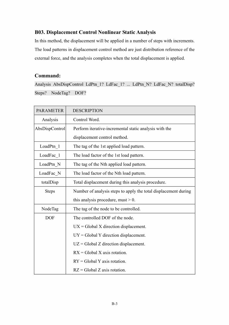
B03. Displacement Control Nonlinear Static Analysis In this method, the displacement will be applied in a number of steps with increments.
The load patterns in displacement control method are just distribution reference of the
external force, and the analysis completes when the total displacement is applied.
Command: Analysis AbsDispControl LdPtn_1? LdFac_1? ... LdPtn_N? LdFac_N? totalDisp?
Steps? NodeTag? DOF?
PARAMETER DESCRIPTION
Analysis Control Word.
AbsDispControl Perform iterative-incremental static analysis with the
displacement control method.
LoadPtn_1 The tag of the 1st applied load pattern.
LoadFac_1 The load factor of the 1st load pattern.
LoadPtn_N The tag of the Nth applied load pattern.
LoadFac_N The load factor of the Nth load pattern.
totalDisp Total displacement during this analysis procedure.
Steps Number of analysis steps to apply the total displacement during
this analysis procedure, must > 0.
NodeTag The tag of the node to be controlled.
DOF The controlled DOF of the node.
UX = Global X direction displacement.
UY = Global Y direction displacement.
UZ = Global Z direction displacement.
RX = Global X axis rotation.
RY = Global Y axis rotation.
RZ = Global Z axis rotation.
B-3
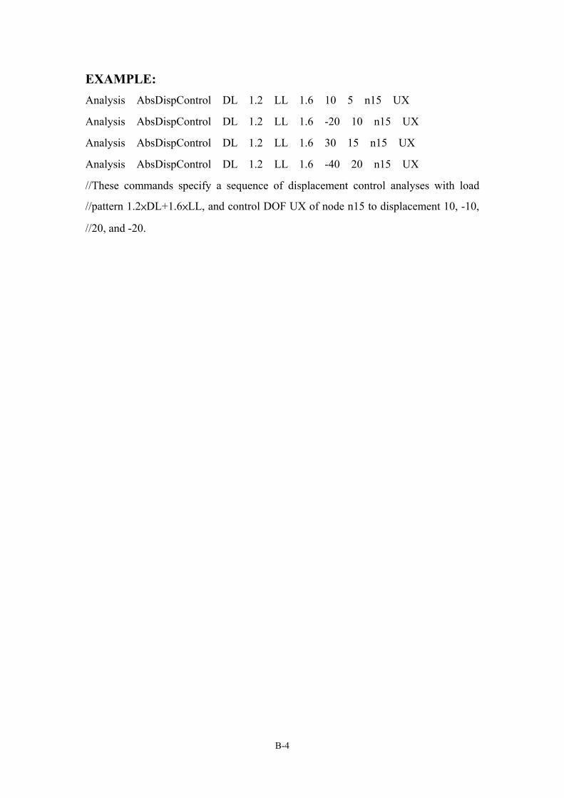
EXAMPLE: Analysis AbsDispControl DL 1.2 LL 1.6 10 5 n15 UX
Analysis AbsDispControl DL 1.2 LL 1.6 -20 10 n15 UX
Analysis AbsDispControl DL 1.2 LL 1.6 30 15 n15 UX
Analysis AbsDispControl DL 1.2 LL 1.6 -40 20 n15 UX
//These commands specify a sequence of displacement control analyses with load
//pattern 1.2×DL+1.6×LL, and control DOF UX of node n15 to displacement 10, -10,
//20, and -20.
B-4
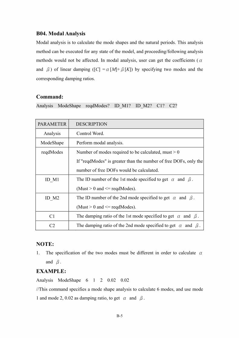
B04. Modal Analysis Modal analysis is to calculate the mode shapes and the natural periods. This analysis
method can be executed for any state of the model, and proceeding/following analysis
methods would not be affected. In modal analysis, user can get the coefficients (α
and β) of linear damping ([C] =α[M]+β[K]) by specifying two modes and the
corresponding damping ratios.
Command: Analysis ModeShape reqdModes? ID_M1? ID_M2? C1? C2?
PARAMETER DESCRIPTION
Analysis Control Word.
ModeShape Perform modal analysis.
reqdModes Number of modes required to be calculated, must > 0
If "reqdModes" is greater than the number of free DOFs, only the
number of free DOFs would be calculated.
ID_M1 The ID number of the 1st mode specified to get α and β.
(Must > 0 and <= reqdModes).
ID_M2 The ID number of the 2nd mode specified to get α and β.
(Must > 0 and <= reqdModes).
C1 The damping ratio of the 1st mode specified to get α and β.
C2 The damping ratio of the 2nd mode specified to get α and β.
NOTE: 1. The specification of the two modes must be different in order to calculate α
and β.
EXAMPLE: Analysis ModeShape 6 1 2 0.02 0.02
//This command specifies a mode shape analysis to calculate 6 modes, and use mode
1 and mode 2, 0.02 as damping ratio, to get α and β.
B-5
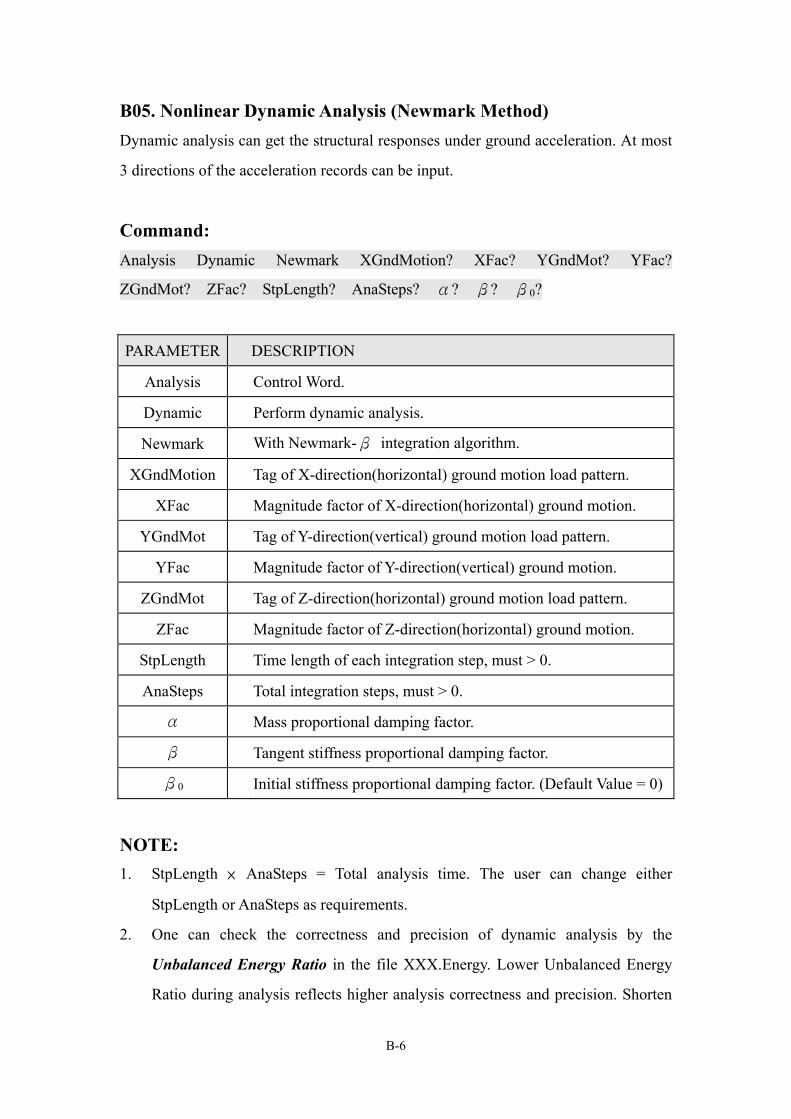
B05. Nonlinear Dynamic Analysis (Newmark Method) Dynamic analysis can get the structural responses under ground acceleration. At most
3 directions of the acceleration records can be input.
Command: Analysis Dynamic Newmark XGndMotion? XFac? YGndMot? YFac?
ZGndMot? ZFac? StpLength? AnaSteps? α? β? β0?
PARAMETER DESCRIPTION
Analysis Control Word.
Dynamic Perform dynamic analysis.
Newmark With Newmark-β integration algorithm.
XGndMotion Tag of X-direction(horizontal) ground motion load pattern.
XFac Magnitude factor of X-direction(horizontal) ground motion.
YGndMot Tag of Y-direction(vertical) ground motion load pattern.
YFac Magnitude factor of Y-direction(vertical) ground motion.
ZGndMot Tag of Z-direction(horizontal) ground motion load pattern.
ZFac Magnitude factor of Z-direction(horizontal) ground motion.
StpLength Time length of each integration step, must > 0.
AnaSteps Total integration steps, must > 0.
α Mass proportional damping factor.
β Tangent stiffness proportional damping factor.
β0 Initial stiffness proportional damping factor. (Default Value = 0)
NOTE: 1. StpLength × AnaSteps = Total analysis time. The user can change either
StpLength or AnaSteps as requirements.
2. One can check the correctness and precision of dynamic analysis by the
Unbalanced Energy Ratio in the file XXX.Energy. Lower Unbalanced Energy
Ratio during analysis reflects higher analysis correctness and precision. Shorten
B-6
StpLength can usually raise the precision, but it will also cost more analysis
duration.
3. If only one or two direction(s) have ground excitation, the ground motion load
pattern of rest direction(s) should input as “None”.
4. The linear structural damping can be modeled as [C] =α[M]+β[Kt], or [C] =α
[M]+β0[K0]. Where [Kt] is the structural tangent stiffness and [K0] is the
structural initial stiffness. The user should choose one of β and β0 to input, or
the damping effects of the structure will be taken into account improperly as β
and β0 are input simultaneously.
EXAMPLE: Analysis Dynamic Newmark EQEW 0.33 none 0 EQSN 0.33 0.04 1000
1.00221388E-001 3.86725431E-003 0
//This command defines a two way (X-dir. and Z-dir.) earthquake analysis.
//Note: This command should occupy one line of the input file.
B-7
B06. Pushover Nonlinear Static Analysis This is an analysis method with displacement-based algorithm. The monitored nodal
displacement will be applied with increments. User can determine the number of steps
to apply the displacement. The specified load patterns are just distribution reference
of the external force, and the analysis completes when the total displacement is
executed. The responses of the analysis model would be output at the first step, final
step, and the steps that the model’s state changes.
Command: Analysis Pushover LdPtn_1? LdFac_1? ...... LdPtn_N? LdFac_N? totalDisp?
Steps? NodeTag? DOF?
PARAMETER DESCRIPTION
Analysis Control Word.
Pushover To perform nonlinear static analysis with the pushover method.
LoadPtn_1 The tag of the 1st applied load pattern.
LoadFac_1 The load factor of the 1st load pattern.
LoadPtn_N The tag of the Nth applied load pattern.
LoadFac_N The load factor of the Nth load pattern.
totalDisp Total displacement of the monitored degree of freedom during
this pushover procedure.
Steps Number of analysis steps to apply the totalDisp during this
pushover procedure, must > 0.
NodeTag The tag of the node to be controlled.
DOF The monitored degree of freedom of the node.
UX = Global X direction displacement.
UY = Global Y direction displacement.
UZ = Global Z direction displacement.
RX = Global X axis rotation.
RY = Global Y axis rotation.
RZ = Global Z axis rotation.
B-8

EXAMPLE: Analysis Pushover Push 1.0 3000 3000 12 Ux
//This command specifies a pushover analysis with load pattern 1.0×push, and
//controls DOF UX of node 12 to go through displacement 3000 with 3000 steps.
B-9
B07. Nonlinear Dynamic Analysis (OS Method) This analysis method can get the structural responses under three-dimensional ground
acceleration. The Operator-Splitting (OS) integration algorithm uses techniques of
merging predictor-corrector / implicit-explicit in nonlinear finite element analysis. It
is confirmed that OS method can save much time and get well analysis accuracy in
dynamic analysis. The associated theories can be detailed in [2] and [3]. This method
of PISA3D is implemented by Yi-Jer Yu ([email protected]).
Command: Analysis Dynamic OS XGndMotion? XFac? YGndMot? YFac? ZGndMot?
ZFac? StpLength? AnaSteps? α? β? β0?
PARAMETER DESCRIPTION
Analysis Control Word.
Dynamic Perform dynamic analysis.
OS With Operator-Splitting integration algorithm.
XGndMotion Tag of X-direction(horizontal) ground motion load pattern.
XFac Magnitude factor of X-direction(horizontal) ground motion.
YGndMot Tag of Y-direction(vertical) ground motion load pattern.
YFac Magnitude factor of Y-direction(vertical) ground motion.
ZGndMot Tag of Z-direction(horizontal) ground motion load pattern.
ZFac Magnitude factor of Z-direction(horizontal) ground motion.
StpLength Time length of each integration step, must > 0.
AnaSteps Total integration steps, must > 0.
α Mass proportional damping factor.
β Tangent stiffness proportional damping factor.
β0 Initial stiffness proportional damping factor. (Default Value = 0)
B-10
NOTE: 1. Currently, the OS integration algorithm can not be applied to “Nonlinear
Damper Element”. (FD=CVη, η is not equal to 1. See Part G05) Therefore, the
analyzed model must not be composed of “Nonlinear Damper Element” or the
analysis result will be incorrect.
2. The OS method provides higher efficiency than the Newmark method does,
especially in the circumstance that the nonlinear behavior of the analysis model
is apparent. Using OS method can save analysis time.
3. One can also check the correctness and precision of dynamic analysis by the
Unbalanced Energy Ratio in the file XXX.Energy. Lower Unbalanced Energy
Ratio during analysis reflects higher analysis correctness and precision. Shorten
StpLength can usually raise the precision, but it will also cost more analysis
duration.
4. If only one or two direction(s) have ground excitation, the ground motion load
pattern of rest direction(s) should input as “None”.
5. The linear structural damping can be modeled as [C] =α[M]+β[Kt], or [C] =α
[M]+β0[K0]. Where [Kt] is the structural tangent stiffness and [K0] is the
structural initial stiffness. The user should choose one of β and β0 to input, or
the damping effects of the structure will be taken into account improperly as β
and β0 are input simultaneously.
EXAMPLE: Analysis Dynamic OS EQEW 0.33 none 0 EQSN 0.33 0.04 1000 1.00221388E-001
3.86725431E-003 0
//This command defines a two-way (X-dir. and Z-dir.) earthquake analysis with OS
integration algorithm.
B-11
PART C. Analysis Control Setting Command
These types of commands control some settings during the analysis procedure.
C01. Geometric Nonlinear Effect This command sets the geometric nonlinear consideration during the analysis
procedure. See Reference [1].
Command: ControlData GeometricNL Code?
PARAMETER DESCRIPTION
ControlData Control Word.
GeometricNL Setting geometric nonlinear effect by geometric stiffness matrix.
Code 0 = Do not consider geometric stiffness matrix (Default Value).
1 = Consider geometric stiffness matrix only after every analysis
method.
2 = Update geometric stiffness matrix before each analysis step
in analysis methods
EXAMPLE: ControlData GeometricNL 1
C-1
PART D. Node Data Command
The following commands are about the nodal data descriptions. Note that all the
nodes must have their unique tags.
D01. Node Generation This command is to define the nodal coordinates.
Command: Node Tag? Coord-X? Coord-Y? Coord-Z?
PARAMETER DESCRIPTION
Node Control Word.
Tag Unique tag of this node.
Coord-X Coordinate of X direction.
Coord-Y Coordinate of Y direction.
Coord-Z Coordinate of Z direction.
(Default Value = 0)
EXAMPLE: Node n1 6928.2 4000.0 1000
D-1
D02. Nodal Degree of Freedom Assign This command defines the restraint of the nodal degree of freedom.
Command: DOF Node? UX? UY? UZ? RX? RY? RZ?
PARAMETER DESCRIPTION
DOF Control Word.
Node Tag of the specified node.
UX Fixity of X-dir. displacement.
-1 = fixed.
0 = free.
other node's tag = identical to the node.
UY Fixity of Y-dir. displacement.
-1 = fixed.
0 = free.
other node's tag = identical to the node.
UZ Fixity of Z-dir. displacement.
-1 = fixed.
0 = free.
other node's tag = identical to the node.
RX Fixity of rotation about the global X-axis.
-1 = fixed.
0 = free.
other node's tag = identical to the node.
RY Fixity of rotation about the global Y-axis.
-1 = fixed.
0 = free.
other node's tag = identical to the node.
D-2
RZ Fixity of rotation about the global Z-axis.
-1 = fixed.
0 = free.
other node's tag = identical to the node.
NOTE: 1. If there are no DOFs assigned for one node, the default DOFs of this node are set
to be all free.
2. If the technique of the same DOFs is used, the identical fixity of the identical
node should be assigned to be free in front.
EXAMPLE: DOF n1 0 0 -1 -1 -1 -1
//This command set dof. UZ, RX, RY, RZ of node n1 to be fixed.
DOF 74 0 0 15 0 -1 0
//This command specifies that dof. UZ of node 74 is equal to dof. UZ of node 15, and
dof. RY is fixed.
D-3
D03. Nodal Lump Mass Assign User can specify the lump mass of a node by this command.
Command: Mass Node? UX? UY? UZ? RX? RY? RZ?
PARAMETER DESCRIPTION
Mass Control Word.
Node Tag of the specified node.
UX Translational mass associated with X-dir. Displacement,
must >= 0. (Default Value = 0)
UY Translational mass associated with Y-dir. Displacement,
must >= 0. (Default Value = 0)
UZ Translational mass associated with Z-dir. Displacement,
must >= 0. (Default Value = 0)
RX Rotational moment of inertia about the global X-axis,
must >= 0. (Default Value = 0)
RY Rotational moment of inertia about the global Y-axis,
must >= 0. (Default Value = 0)
RZ Rotational moment of inertia about the global Z-axis,
must >= 0. (Default Value = 0)
NOTE: 1. If there are no lump mass assigned for one node, the default lump mass of this
node is set to be all zero.
EXAMPLE: Mass 2 10 10 10 0 0 0
D-4
D04. Nodal Linear Spring This command allows the user to define the fully-coupled 6-by-6 stiffness spring of
any node.
Command: Spring NodeTag? Kux? Kuy? Kuz? Krx? Kry? Krz? ... <KMN? ValueKMN?>
PARAMETER DESCRIPTION
Spring Control Word.
NodeTag Tag of the specified node.
Kux Spring stiffness in global X axis. (Default = 0)
Kuy Spring stiffness in global Y axis. (Default = 0)
Kuz Spring stiffness in global Z axis. (Default = 0)
Krx Spring rotational stiffness about global X axis. (Default = 0)
Kry Spring rotational stiffness about global Y axis. (Default = 0)
Krz Spring rotational stiffness about global Z axis. (Default = 0)
KMN Identify the DOF for off-diagonal spring.
M can be ux, uy, uz, rx, ry, rz.
N can be ux, uy, uz, rx, ry, rz.
Ex: Kuzry means the next spring stiffness value is for UZRY.
ValueKMN Spring stiffness value of above-mentioned DOF KMN.
NOTE: 1. <KMN? ValueKMN?> is optional, at most the 15 off-diagonal spring stiffness
can be all defined, and the default values are all 0.
EXAMPLE: Spring N5 0 0 1E5 0 1E3 1000 Kuzrz 300
//This command specifies node N5 with spring value: KUZ=100000, KRY=KRZ=1000, KUZRZ=300 and others=0
D-5
D05. Constraint Definition (Rigid Diaphragm) This command is to specify the rigid floors of a 3D-building. See Fig. D01. Each floor
should be defined as a unique rigid diaphragm, and the center of floor’s mass is the
master node.
Command: Constraint Diaphragm Tag? MasterNd? SlaveNd1? ... SlaveNdN? ...<S NF? NL?>
PARAMETER DESCRIPTION
Constraint Control Word.
Diaphragm Rigid diaphragm for building system.
Tag Unique tag of this diaphragm.
MasterNd Tag of the master node.
SlaveNd1 Tag of the slaved node 1.
SlaveNdN Tag of the slaved node N.
S To indicate sequential generation of slaved nodes.
NF Numeral tag of the first slaved node.
NL Numeral tag of the last slaved node.
NOTE: 1. The DOF UX/UZ/RY of the master node and the slaved nodes must be free, and
the master node can not itself be slaved.
(i.e. More than one diaphragm can exist at the same level, but only single slaving
is permitted for each slaved node.)
2. <S NF? NL?> is optional for the identification of slaved nodes.
If "S" is input in this command, the 1st and 2nd following nodal tags must be
numerals, and the slaved nodes would be generated node by node automatically.
D-6
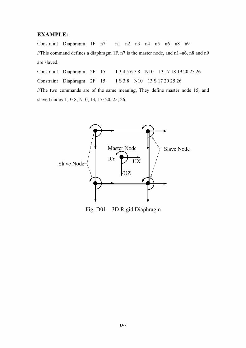
EXAMPLE: Constraint Diaphragm 1F n7 n1 n2 n3 n4 n5 n6 n8 n9
//This command defines a diaphragm 1F. n7 is the master node, and n1~n6, n8 and n9
are slaved.
Constraint Diaphragm 2F 15 1 3 4 5 6 7 8 N10 13 17 18 19 20 25 26
Constraint Diaphragm 2F 15 1 S 3 8 N10 13 S 17 20 25 26
//The two commands are of the same meaning. They define master node 15, and
slaved nodes 1, 3~8, N10, 13, 17~20, 25, 26.
Fig. D01 3D Rigid Diaphragm
D-7
PART E. Load Pattern Command
E01. Nodal Load This command defines static nodal loads. Various nodal load commands can have the
same tag. These commands would be combined as a single load pattern automatically.
If commands have different tags, they would be taken as different patterns.
Command: LoadPattern NodalLoad Tag? Node? FX? FY? FZ? MX? MY? MZ?
PARAMETER DESCRIPTION
LoadPattern Control Word.
NodalLoad Nodal external load.
Tag Tag of this load pattern.
Node Tag of the target node.
FX External force on the X direction.
FY External force on the Y direction.
FZ External force on the Z direction.
MX External moment about the global X axis.
(Counterclockwise as positive by normal view to the X axis.)
MY External moment about the global Y axis.
(Counterclockwise as positive by normal view to the Y axis.)
MZ External moment about the global Z axis.
(Counterclockwise as positive by normal view to the Z axis.)
EXAMPLE: LoadPattern NodalLoad DL n1 383 321.4 0 0 0 0
LoadPattern NodalLoad DL n2 -15 0 130 0 200 0
//Using two commands to define a load pattern named DL.
E-1
E02. Ground Acceleration Record In this command, the corresponding acceleration record file should be prepared. The
dynamic analysis would use the acceleration record as the ground excitation. Different
records should have different tags, or the previous one will be replaced.
Command: LoadPattern GroundAccel Tag? FileName? TimeFactor? MagnFactor?
PARAMETER DESCRIPTION
LoadPattern Control Word.
GroundAccel Ground motion as time-history of acceleration.
Tag Tag of this load pattern.
FileName File name of the time-history record file, which is in relative path
to the input file.
TimeFactor Time scale factor, must > 0.
(Default Value = 1.0)
MagnFactor Magnitude scale factor.
(Default Value = 1.0)
NOTE: 1. The acceleration record file must be in two columns text format. The first
column is time and the second column is the corresponding acceleration value.
EXAMPLE: LoadPattern GroundAccel EQX CHY076EW.txt 1 9.81
//This command defines an acceleration time history named EQX, and the record file is put in the same folder as the input file.
E-2
PART F. Material Definition Command
All the different material objects should have their own tags, even if the types of
materials are different. For many elements use an identical material, only one material
command for this material is needed. The program will generate the material copies
for the elements. This concept is similar to many analysis programs, like SAP and
ETABS.
F01. Elastic Material This material would always keep linear elastic. See Fig. F01 for the elastic material.
Command: Material Elastic Tag? E? Nu?
PARAMETER DESCRIPTION
Material Control Word.
Elastic Elastic material without yielding state.
Tag Unique tag of this material.
E Young's modulus.
Nu Poisson Ratio, must between 0 and 0.5.
(Default Value = 0)
States of the Material: One can check the material yielding state in the output of the element which uses this material.
CODE STATE DESCRIPTION
0 Linear This material always keeps linear elastic state.
F-1
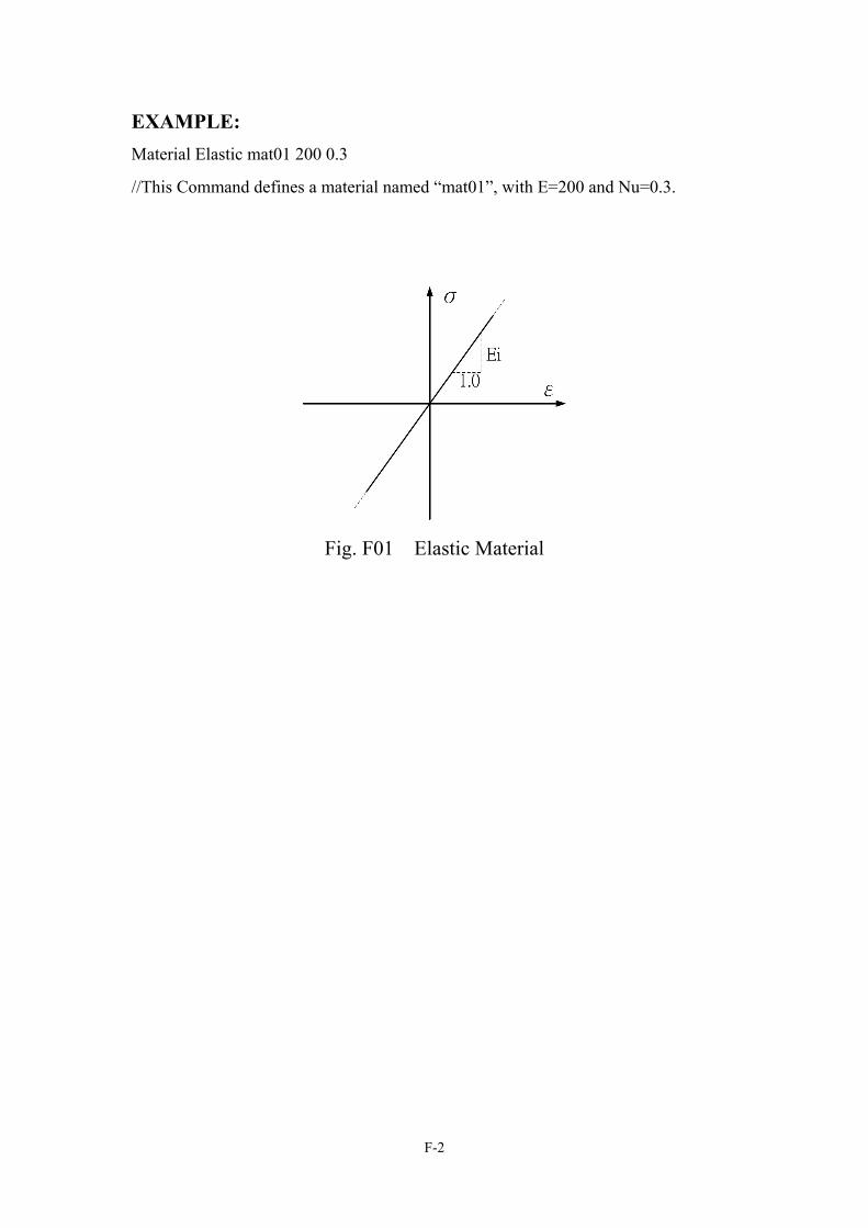
EXAMPLE: Material Elastic mat01 200 0.3
//This Command defines a material named “mat01”, with E=200 and Nu=0.3.
Fig. F01 Elastic Material
F-2
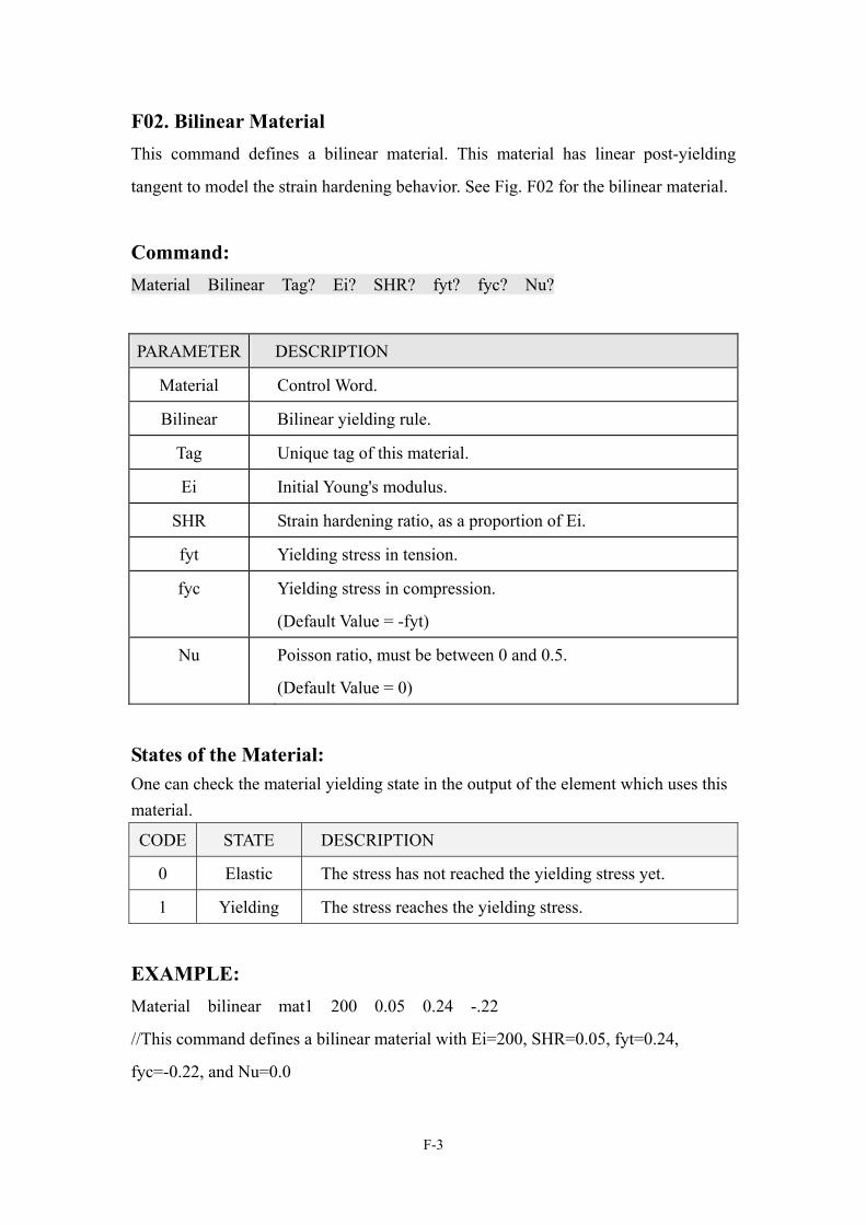
F02. Bilinear Material This command defines a bilinear material. This material has linear post-yielding
tangent to model the strain hardening behavior. See Fig. F02 for the bilinear material.
Command: Material Bilinear Tag? Ei? SHR? fyt? fyc? Nu?
PARAMETER DESCRIPTION
Material Control Word.
Bilinear Bilinear yielding rule.
Tag Unique tag of this material.
Ei Initial Young's modulus.
SHR Strain hardening ratio, as a proportion of Ei.
fyt Yielding stress in tension.
fyc Yielding stress in compression.
(Default Value = -fyt)
Nu Poisson ratio, must be between 0 and 0.5.
(Default Value = 0)
States of the Material: One can check the material yielding state in the output of the element which uses this material.
CODE STATE DESCRIPTION
0 Elastic The stress has not reached the yielding stress yet.
1 Yielding The stress reaches the yielding stress.
EXAMPLE: Material bilinear mat1 200 0.05 0.24 -.22
//This command defines a bilinear material with Ei=200, SHR=0.05, fyt=0.24,
fyc=-0.22, and Nu=0.0
F-3
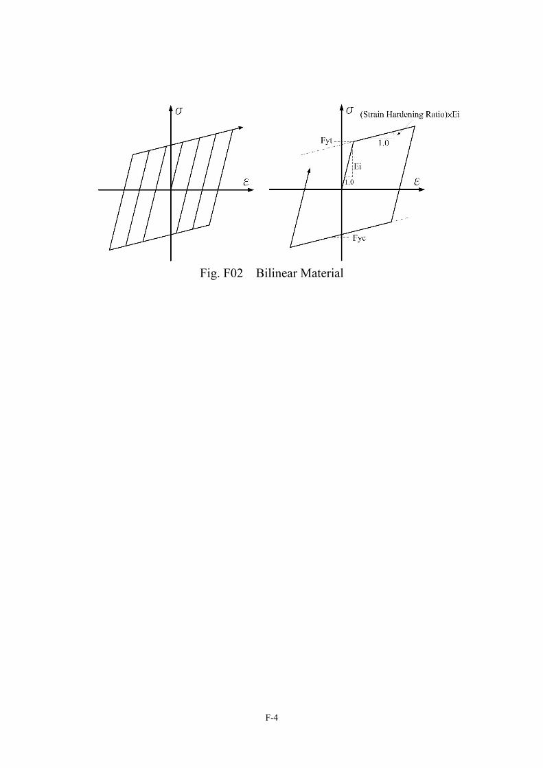
Fig. F02 Bilinear Material
F-4
F03. Hardening Material This material adopts two-surface plastic hardening rule. See Fig. F03 and Fig. F04 for
the hardening material. This material is usually used to model the metal material
precisely. Take reference to [1].
Command: Material Hardening Tag? Ei? fyt? fyc? Hiso1+? Hiso2+? Hiso1-? Hiso2-?
Hkin1? Hkin2? B/Y? Nu? subStep?
PARAMETER DESCRIPTION
Material Control Word.
Hardening Two surface hardening rule.
Tag Unique tag of this material.
Ei Initial Young's modulus.
fyt Yielding stress in tension.
fyc Yielding stress in compression.
Hiso1+ Positive isotropic hardening parameter C1.
Hiso2+ Positive isotropic hardening parameter C2.
Hiso1- Negative isotropic hardening parameter C1.
(Default Value = Hiso1+)
Hiso2- Negative isotropic hardening parameter C2.
(Default Value = Hiso2+)
Hkin1 Kinematic hardening parameter C3.
(Default Value = 1.0)
Hkin2 Kinematic hardening parameter C4.
(Default Value = 10.0)
B/Y Initial ratio of the two surfaces (Boundary/Yielding, i.e. BS/YS).
(Default Value = 1.0)
Nu Poisson Ratio, must between 0 and 0.5.
(Default Value = 0)
F-5
subStep Steps of strain incremental segment in yielding state.
(Default Value = 10)
States of the Material: One can check the material yielding state in the output of the element which uses this material.
CODE STATE DESCRIPTION
0 Elastic The stress has not reached the yielding stress yet.
1 Kinematic
Hardening
The stress reaches the yielding surface but below the
boundary surface, and keeps kinematic hardening.
2 Isotropic
Hardening
The stress reaches the boundary surface, and keeps both
isotropic hardening and kinematic hardening.
NOTE: 1. More “subStep” will waste more analysis time, but it will also improve the
analysis correctness and reduce the possibility of converge failure.
EXAMPLE: Material Hardening 2 200 0.24 -0.24 0.0045 2.8 .009 2.8 1.0 24 1.3 0.3 100
Fig. F03 Hardening Material
F-6
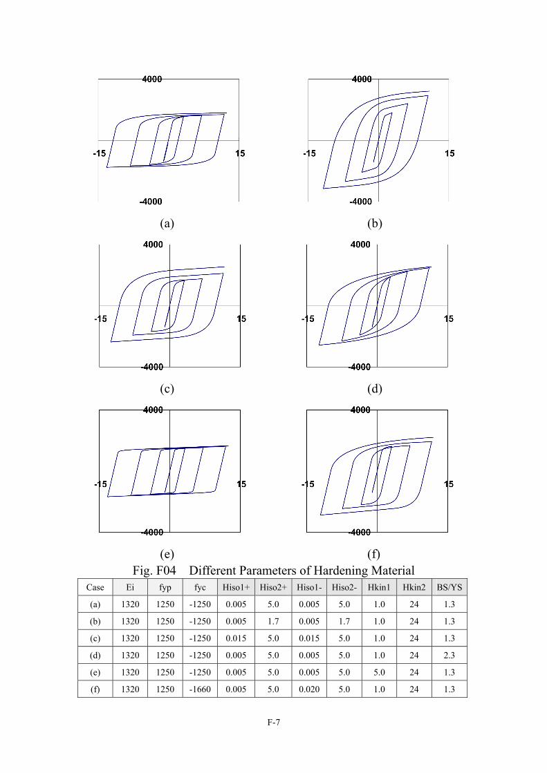
(a) (b)
(c) (d)
(e) (f) Fig. F04 Different Parameters of Hardening Material
Case Ei fyp fyc Hiso1+ Hiso2+ Hiso1- Hiso2- Hkin1 Hkin2 BS/YS
(a) 1320 1250 -1250 0.005 5.0 0.005 5.0 1.0 24 1.3
(b) 1320 1250 -1250 0.005 1.7 0.005 1.7 1.0 24 1.3
(c) 1320 1250 -1250 0.015 5.0 0.015 5.0 1.0 24 1.3
(d) 1320 1250 -1250 0.005 5.0 0.005 5.0 1.0 24 2.3
(e) 1320 1250 -1250 0.005 5.0 0.005 5.0 5.0 24 1.3
(f) 1320 1250 -1660 0.005 5.0 0.020 5.0 1.0 24 1.3
F-7
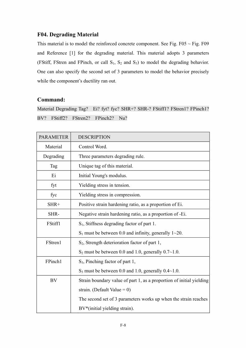
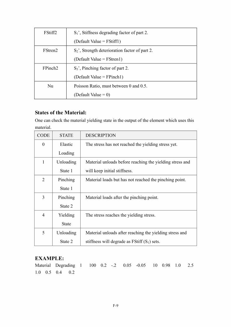
F04. Degrading Material This material is to model the reinforced concrete component. See Fig. F05 ~ Fig. F09
and Reference [1] for the degrading material. This material adopts 3 parameters
(FStiff, FStren and FPinch, or call S1, S2 and S3) to model the degrading behavior.
One can also specify the second set of 3 parameters to model the behavior precisely
while the component’s ductility ran out.
Command:
Material Degrading Tag? Ei? fyt? fyc? SHR+? SHR-? FStiff1? FStren1? FPinch1?
BV? FStiff2? FStren2? FPinch2? Nu?
PARAMETER DESCRIPTION
Material Control Word.
Degrading Three parameters degrading rule.
Tag Unique tag of this material.
Ei Initial Young's modulus.
fyt Yielding stress in tension.
fyc Yielding stress in compression.
SHR+ Positive strain hardening ratio, as a proportion of Ei.
SHR- Negative strain hardening ratio, as a proportion of -Ei.
FStiff1 S1, Stiffness degrading factor of part 1.
S1 must be between 0.0 and infinity, generally 1~20.
FStren1 S2, Strength deterioration factor of part 1,
S2 must be between 0.0 and 1.0, generally 0.7~1.0.
FPinch1 S3, Pinching factor of part 1,
S3 must be between 0.0 and 1.0, generally 0.4~1.0.
BV Strain boundary value of part 1, as a proportion of initial yielding
strain. (Default Value = 0)
The second set of 3 parameters works up when the strain reaches
BV*(initial yielding strain).
F-8
FStiff2 S1’, Stiffness degrading factor of part 2.
(Default Value = FStiff1)
FStren2 S2’, Strength deterioration factor of part 2.
(Default Value = FStren1)
FPinch2 S3’, Pinching factor of part 2.
(Default Value = FPinch1)
Nu Poisson Ratio, must between 0 and 0.5.
(Default Value = 0)
States of the Material: One can check the material yielding state in the output of the element which uses this material.
CODE STATE DESCRIPTION
0 Elastic
Loading
The stress has not reached the yielding stress yet.
1 Unloading
State 1
Material unloads before reaching the yielding stress and
will keep initial stiffness.
2 Pinching
State 1
Material loads but has not reached the pinching point.
3 Pinching
State 2
Material loads after the pinching point.
4 Yielding
State
The stress reaches the yielding stress.
5 Unloading
State 2
Material unloads after reaching the yielding stress and
stiffness will degrade as FStiff (S1) sets.
EXAMPLE: Material Degrading 1 100 0.2 -.2 0.05 -0.05 10 0.98 1.0 2.5 1.0 0.5 0.4 0.2
F-9
Fig. F05a Degrading Material
Fig. F05b States of Degrading Material
Fig. F06 Stiffness Degrading Factor
F-10
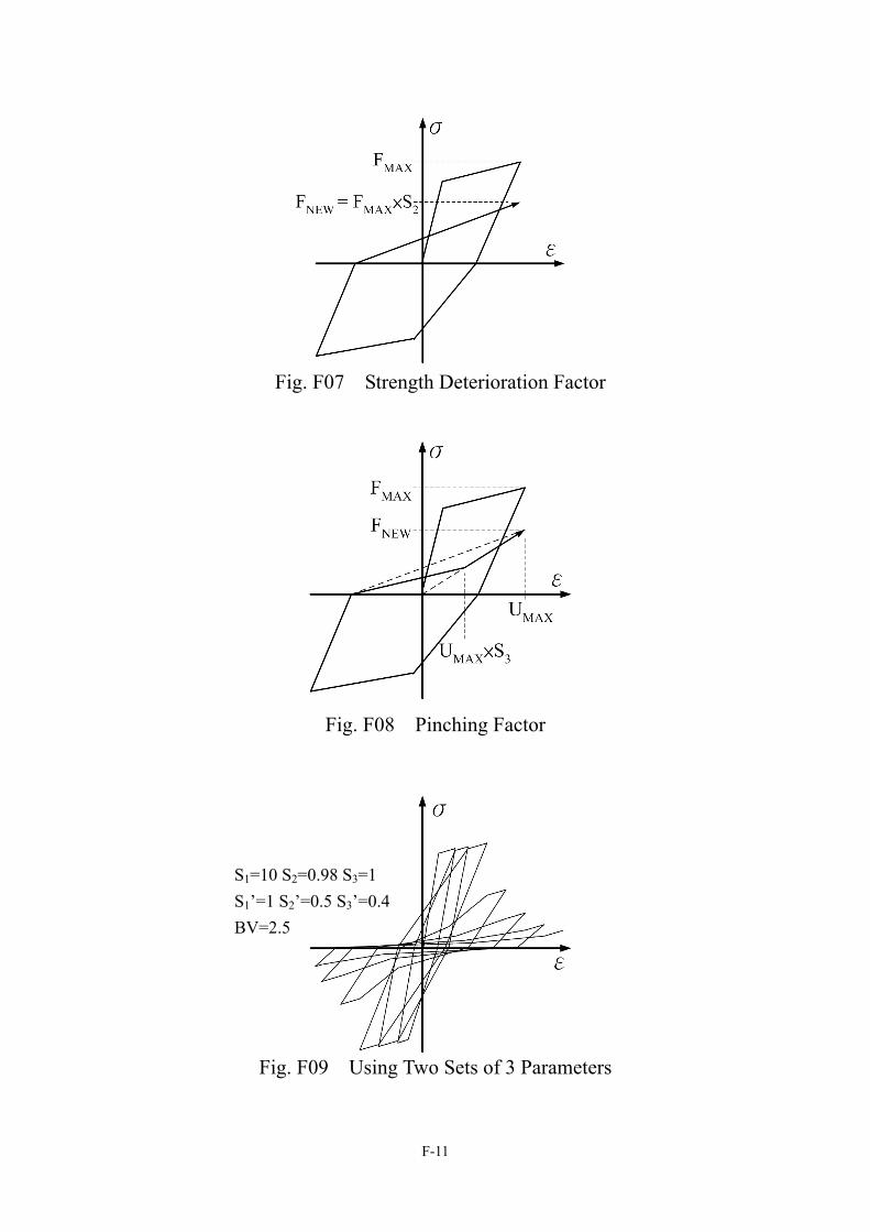
Fig. F07 Strength Deterioration Factor
Fig. F08 Pinching Factor
S1=10 S2=0.98 S3=1 S1’=1 S2’=0.5 S3’=0.4BV=2.5
Fig. F09 Using Two Sets of 3 Parameters
F-11
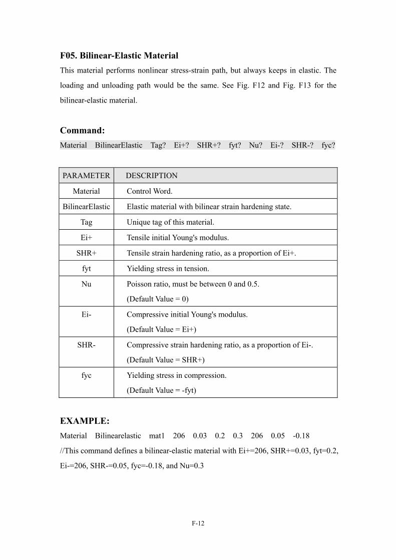
F05. Bilinear-Elastic Material This material performs nonlinear stress-strain path, but always keeps in elastic. The
loading and unloading path would be the same. See Fig. F12 and Fig. F13 for the
bilinear-elastic material.
Command: Material BilinearElastic Tag? Ei+? SHR+? fyt? Nu? Ei-? SHR-? fyc?
PARAMETER DESCRIPTION
Material Control Word.
BilinearElastic Elastic material with bilinear strain hardening state.
Tag Unique tag of this material.
Ei+ Tensile initial Young's modulus.
SHR+ Tensile strain hardening ratio, as a proportion of Ei+.
fyt Yielding stress in tension.
Nu Poisson ratio, must be between 0 and 0.5.
(Default Value = 0)
Ei- Compressive initial Young's modulus.
(Default Value = Ei+)
SHR- Compressive strain hardening ratio, as a proportion of Ei-.
(Default Value = SHR+)
fyc Yielding stress in compression.
(Default Value = -fyt)
EXAMPLE: Material Bilinearelastic mat1 206 0.03 0.2 0.3 206 0.05 -0.18
//This command defines a bilinear-elastic material with Ei+=206, SHR+=0.03, fyt=0.2,
Ei-=206, SHR-=0.05, fyc=-0.18, and Nu=0.3
F-12
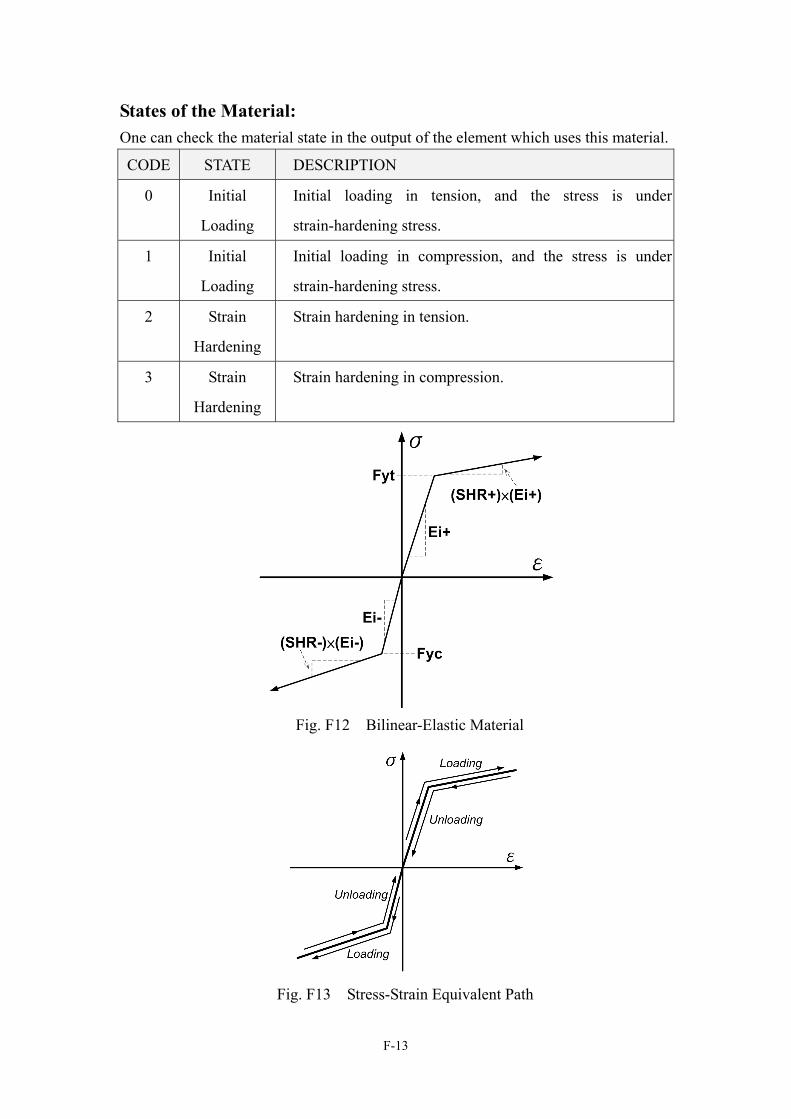
States of the Material: One can check the material state in the output of the element which uses this material.
CODE STATE DESCRIPTION
0 Initial
Loading
Initial loading in tension, and the stress is under
strain-hardening stress.
1 Initial
Loading
Initial loading in compression, and the stress is under
strain-hardening stress.
2 Strain
Hardening
Strain hardening in tension.
3 Strain
Hardening
Strain hardening in compression.
Fig. F12 Bilinear-Elastic Material
Fig. F13 Stress-Strain Equivalent Path
F-13
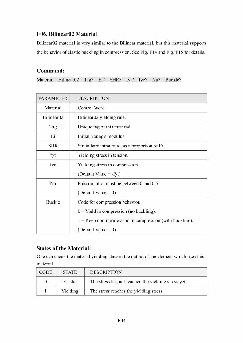
F06. Bilinear02 Material Bilinear02 material is very similar to the Bilinear material, but this material supports
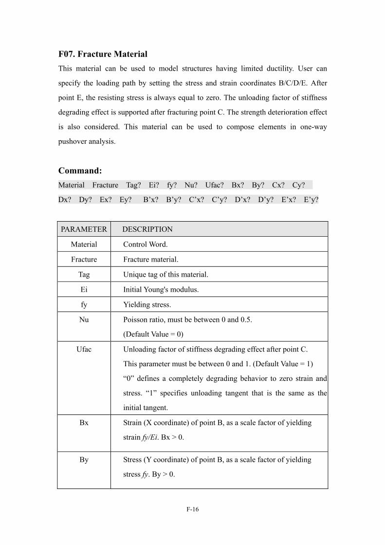
the behavior of elastic buckling in compression. See Fig. F14 and Fig. F15 for details.
Command: Material Bilinear02 Tag? Ei? SHR? fyt? fyc? Nu? Buckle?
PARAMETER DESCRIPTION
Material Control Word.
Bilinear02 Bilinear02 yielding rule.
Tag Unique tag of this material.
Ei Initial Young's modulus.
SHR Strain hardening ratio, as a proportion of Ei.
fyt Yielding stress in tension.
fyc Yielding stress in compression.
(Default Value = -fyt)
Nu Poisson ratio, must be between 0 and 0.5.
(Default Value = 0)
Buckle Code for compression behavior.
0 = Yield in compression (no buckling).
1 = Keep nonlinear elastic in compression (with buckling).
(Default Value = 0)
States of the Material: One can check the material yielding state in the output of the element which uses this material.
CODE STATE DESCRIPTION
0 Elastic The stress has not reached the yielding stress yet.
1 Yielding The stress reaches the yielding stress.
F-14
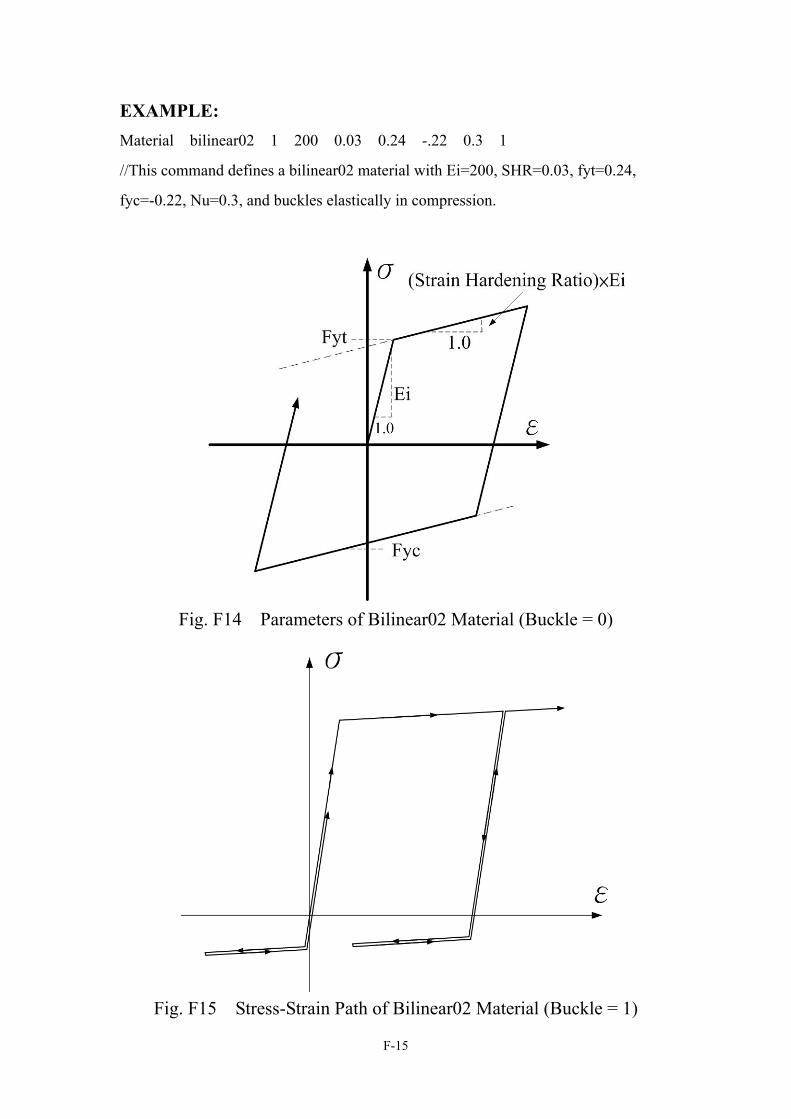
EXAMPLE: Material bilinear02 1 200 0.03 0.24 -.22 0.3 1
//This command defines a bilinear02 material with Ei=200, SHR=0.03, fyt=0.24,
fyc=-0.22, Nu=0.3, and buckles elastically in compression.
Fig. F14 Parameters of Bilinear02 Material (Buckle = 0)
Fig. F15 Stress-Strain Path of Bilinear02 Material (Buckle = 1)
F-15
F07. Fracture Material This material can be used to model structures having limited ductility. User can
specify the loading path by setting the stress and strain coordinates B/C/D/E. After
point E, the resisting stress is always equal to zero. The unloading factor of stiffness
degrading effect is supported after fracturing point C. The strength deterioration effect
is also considered. This material can be used to compose elements in one-way
pushover analysis.
Command:
Material Fracture Tag? Ei? fy? Nu? Ufac? Bx? By? Cx? Cy?
Dx? Dy? Ex? Ey? B’x? B’y? C’x? C’y? D’x? D’y? E’x? E’y?
PARAMETER DESCRIPTION
Material Control Word.
Fracture Fracture material.
Tag Unique tag of this material.
Ei Initial Young's modulus.
fy Yielding stress.
Nu Poisson ratio, must be between 0 and 0.5.
(Default Value = 0)
Ufac Unloading factor of stiffness degrading effect after point C.
This parameter must be between 0 and 1. (Default Value = 1)
“0” defines a completely degrading behavior to zero strain and
stress. “1” specifies unloading tangent that is the same as the
initial tangent.
Bx Strain (X coordinate) of point B, as a scale factor of yielding
strain fy/Ei. Bx > 0.
By Stress (Y coordinate) of point B, as a scale factor of yielding
stress fy. By > 0.
F-16
Cx Strain (X coordinate) of point C, as a scale factor of yielding
strain fy/Ei. Cx > 0.
Cy Stress (Y coordinate) of point C, as a scale factor of yielding
stress fy. Cy > 0.
Dx Strain (X coordinate) of point D, as a scale factor of yielding
strain fy/Ei. Dx > 0.
Dy Stress (Y coordinate) of point D, as a scale factor of yielding
stress fy. Dy > 0.
Ex Strain (X coordinate) of point E, as a scale factor of yielding
strain fy/Ei. Ex > 0.
Ey Stress (Y coordinate) of point E, as a scale factor of yielding
stress fy. Ey > 0.
B’x Strain (X coordinate) of point B’, as a scale factor of yielding
strain fy/Ei. B’x < 0, default value = -Bx.
B’y Stress (Y coordinate) of point B’, as a scale factor of yielding
stress fy. B’y < 0, default value = -By.
C’x Strain (X coordinate) of point C’, as a scale factor of yielding
strain fy/Ei. C’x < 0, default value = -Cx.
C’y Stress (Y coordinate) of point C’, as a scale factor of yielding
stress fy. C’y < 0, default value = -Cy
D’x Strain (X coordinate) of point D’, as a scale factor of yielding
strain fy/Ei. D’x < 0, default value = -Dx.
D’y Stress (Y coordinate) of point D’, as a scale factor of yielding
stress fy. D’y < 0, default value = -Dy.
E’x Strain (X coordinate) of point E’, as a scale factor of yielding
strain fy/Ei. E’x < 0, default value = -Ex.
E’y Stress (Y coordinate) of point E’, as a scale factor of yielding
stress fy. E’y < 0, default value = -Ey.
F-17
F-18
States of the Material: One can check the material states in the element output which uses this material.
CODE STATE DESCRIPTION
0 Elastic
loading/unloading
The stress has not reached the yielding stress yet.
1 Yielding The stress reaches the yielding stress.
2 Fracturing state The strain exceeds the first fracturing point C, but is
under point D.
3 Fracturing state The strain exceeds the second fracturing point D, but
is under point E.
4 Fracturing state The strain exceeds the third fracturing point F, but
the stress has not dropped to zero.
5 Fracturing state Completely fracture state, zero strength.
6 Unloading/reloading
after fracturing
Unloading and reloading after point C, with
unloading factor Ufac.
7 Loading state Loading after unloading from State 6 to zero stress.
NOTE: 1. The horizontal coordinate of point D must be no less than that of point C. And a
too steep behavior between C and D sometimes would cause converging failure
in BeamColumn. Modifying the coordinates slightly can improve this situation.
For example, modify C(6,1.25)/D(6,0.2) to C(6,1.25)/D(6.1,0.2).
EXAMPLE: //See Fig. F16
Material Fracture mat1 200 0.24 0.3 1.0 1 1 6 1.25 6 0.2 8 0.2
//See Fig. F17
Material Fracture mat2 200 0.24 0.3 0.5 1 1 6 1.25 7 0.25 10 0.25
//See Fig. F18 and Fig. F19
Material Fracture mat3 200 0.24 0.3 .85 1 1 6 1.15 6.5 0.25 8 0.25
//See Fig. F20
Material Fracture 4 200 0.24 0.3 0.85 1 1 6 1.25 6 0.2 8 0.2 -1 -1 -1 -1 -1 -0.2 -4 -0.2
//See Fig. F21
Material Fracture 5 200 0.24 0.3 1.0 1 1 4 1.15 6 1.2 8 1.2 -1 -1 -4 -1.15 -6 -1.2 -8 -0.2
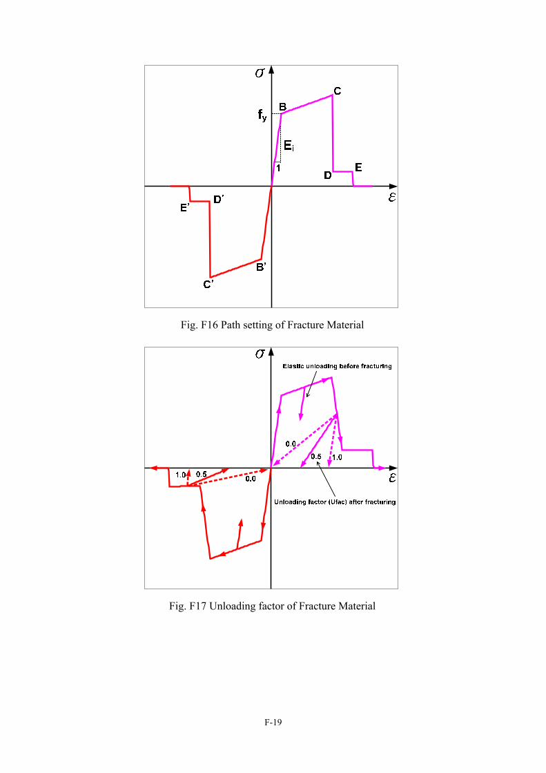
Fig. F16 Path setting of Fracture Material
Fig. F17 Unloading factor of Fracture Material
F-19
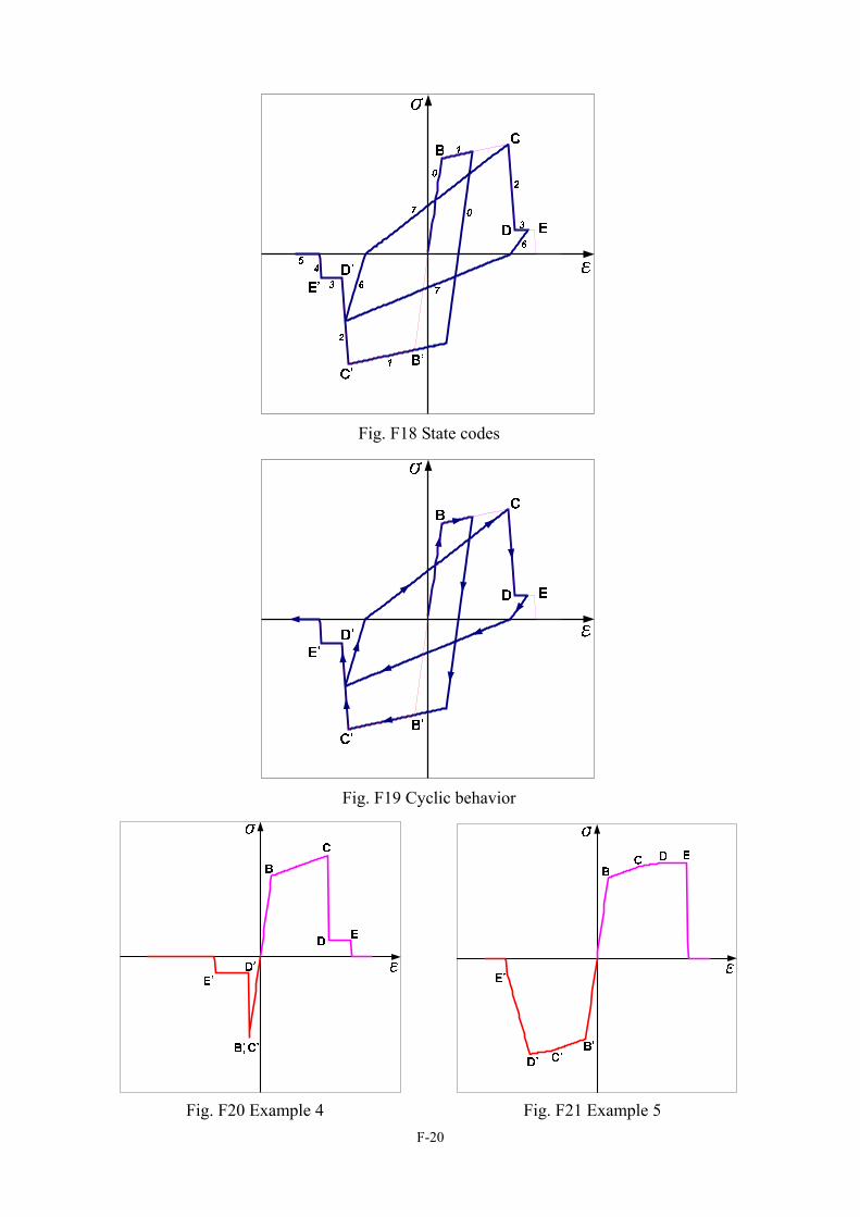
Fig. F18 State codes
Fig. F19 Cyclic behavior
Fig. F20 Example 4 Fig. F21 Example 5
F-20
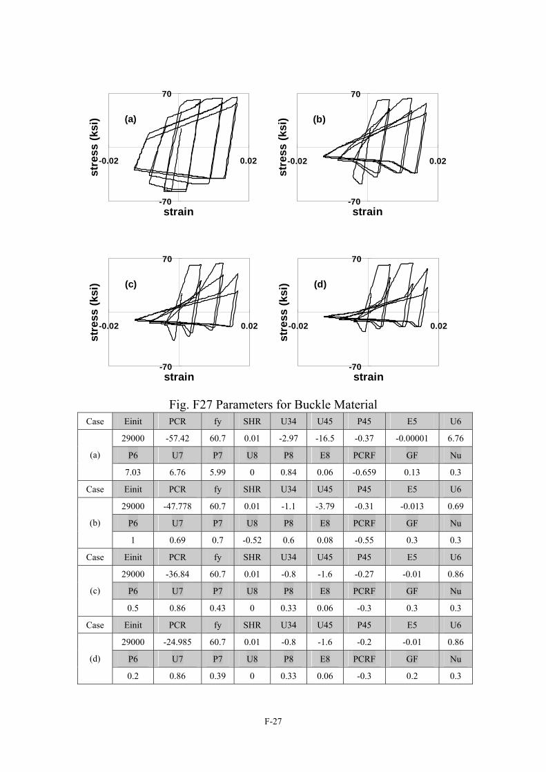
F08. Buckle Material This material is used to model the brace buckling behavior of brace frames and it’s
based on phenomenological brace models theory which predefine the shape of axial
force – axial displacement response. The brace which this material is specified to is
assumed to be pin-ended (see Fig. F22), this implies flexural stiffness of brace is
negligible and rotation at the structural joints where the element is connected have no
influence on the axial force – axial displacement hysteresis rule. References are given
in [Maison and Popov, 1980].
The axial force – axial displacement algorithm simulates the buckling behavior with
nine piecewise lines. Users could specify the values of control points and control
slope to simulate the hysteretic loop (see Fig. F23, Fig. F24). Three additional rules
regarding modifications to the hysteretic behavior due to cyclic loading are:
(a) The strain control points are shifted by δy on unloading from state 2 or 9 (see Fig.
F25). This rule produces a hysteretic loop translation.
(b) A reduction in the compressive strength dependent on inelastic cycling. In the
brace lengthening from state 4, the compressive strength for the next cycle will be
the state 4 compressive stress at which the brace lengthening occurred. On
entering state 5 the compressive strength will be reduced in future cycle to final
compressive strength PCRF. Users could select PCRF to limit the amount of
strength reduction (see Fig. F26).
(c) An inelastic lengthening of the brace at tensile loads less than the uniaxial yield
force after inelastic compressive cycling (column growth). The algorithm will
translate the control strain U29 a ratio of the amount of inelastic shortening in the
previous cycle (see Fig. F26). Users could select GF (growth factor) to simulate
column growth phenomenon.
See Fig. F27 for Buckle Material parameters.
F-21
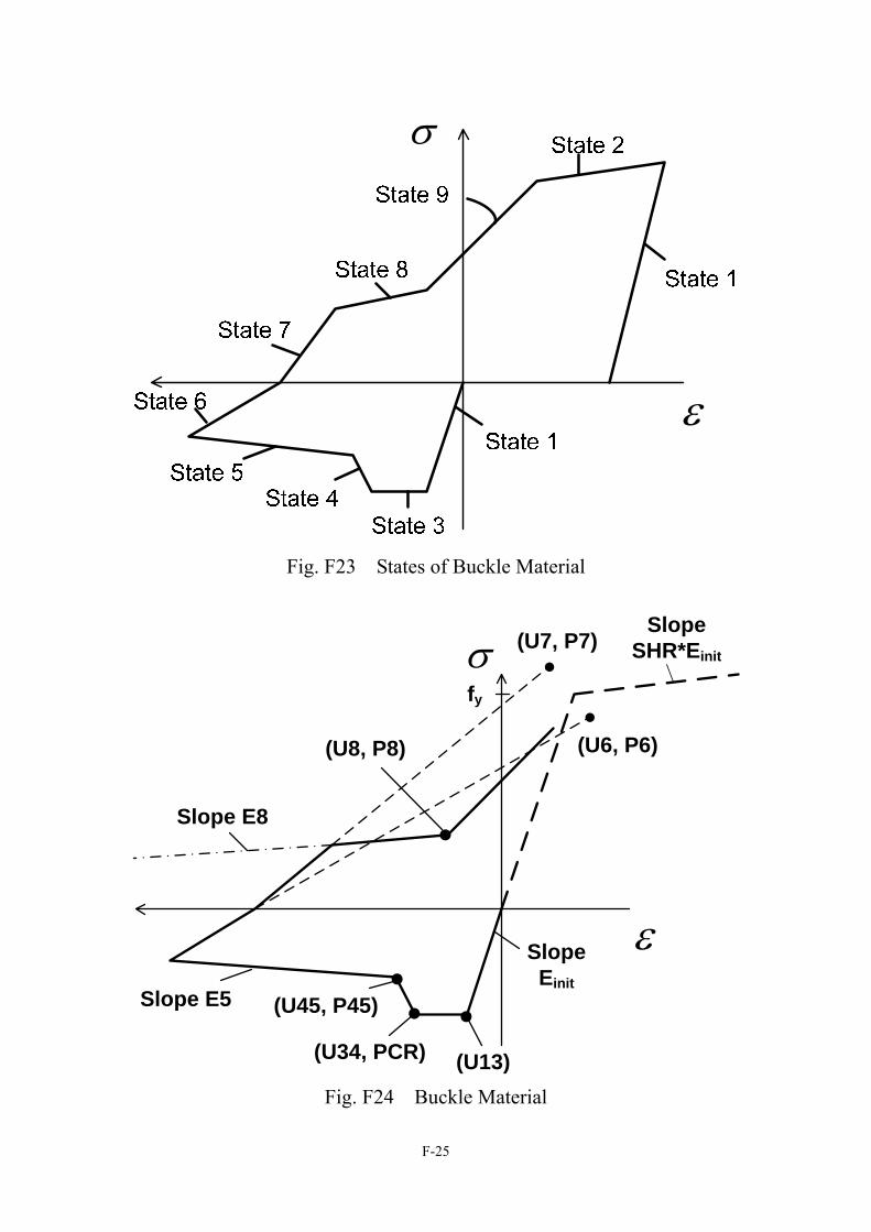
Command: Material Buckle Tag? Einit? PCR? fy? SHR? U34? U45? P45? E5?
U6? P6? U7? P7? U8? P8? E8? PCRF? GF? Nu?
PARAMETER DESCRIPTION
Material Control Word.
Buckle Buckle Material
Tag Unique tag of this material.
Einit Initial Young's modulus.
PCR Buckling strength.
fy Yielding stress in tension.
SHR Strain hardening ratio, as a proportion of Einit.
U34 Strain at intersection of state 3 and 4, as a scale factor of yielding
strain fy/Einit.
U45 Strain at intersection of state 4 and 5, as a scale factor of yielding
strain fy/Einit.
P45 Stress at intersection of state 4 and 5, as a scale factor of yielding
stress fy.
E5 Slope of state 5, as a scale factor of Einit.
U6 Strain of control point for state 6, as a scale factor of yielding
strain fy/Einit.
P6 Stress of control point for state 6, as a scale factor of yielding
stress fy.
U7 Strain of control point for state 7, as a scale factor of yielding
strain fy/Einit.
P7 Stress of control point for state 7, as a scale factor of yielding
stress fy..
U8 Strain of control point for state 8, as a scale factor of yielding
strain fy/Einit.
P8 Stress of control point for state 8, as a scale factor of yielding
F-22
stress fy.
E8 Slope of state 8, as a scale factor of Einit.
PCRF Final buckling strength, as a scale factor of yielding stress fy.
GF Growth factor.
Nu Poisson ratio, must be between 0 and 0.5.
(Default Value = 0)
States of the Material: One can check the material yielding state in the output of the element which uses this material.
CODE STATE DESCRIPTION
1 Elastic
Loading/Unloading
The stress has not reached the yielding stress or
bucking stress yet.
State 1 may exit to state 2 or 3.
2 Hardening The stress reaches the yielding stress.
State 2 may exit to state 1.
3 Buckle The compression stress reaches the buckling
strength.
State 3 may exit to state 4 or 6.
4 Loading in
Compression
Continue loading in compression, and compressive
resistance drops.
State 4 may exit to state 5 or 6.
5 Loading in
Compression
Continue loading in compression, and compressive
resistance drops
State 5 may exit to state 6.
6 Unloading after
buckling
Unloading from state 3, 4, or 5 to zero stress.
State 6 may exit to state 5,7,9,1,3,4.
7 Loading in Tenson Loading in tension.
State 7 may exit to state 6,8,9.
F-23
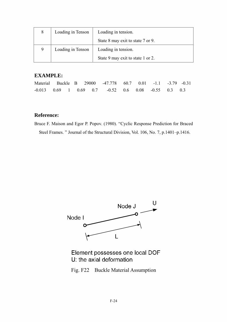
8 Loading in Tenson Loading in tension.
State 8 may exit to state 7 or 9.
9 Loading in Tenson Loading in tension.
State 9 may exit to state 1 or 2.
EXAMPLE: Material Buckle B 29000 -47.778 60.7 0.01 -1.1 -3.79 -0.31 -0.013 0.69 1 0.69 0.7 -0.52 0.6 0.08 -0.55 0.3 0.3
Reference: Bruce F. Maison and Egor P. Popov. (1980). “Cyclic Response Prediction for Braced
Steel Frames. ” Journal of the Structural Division, Vol. 106, No. 7, p.1401–p.1416.
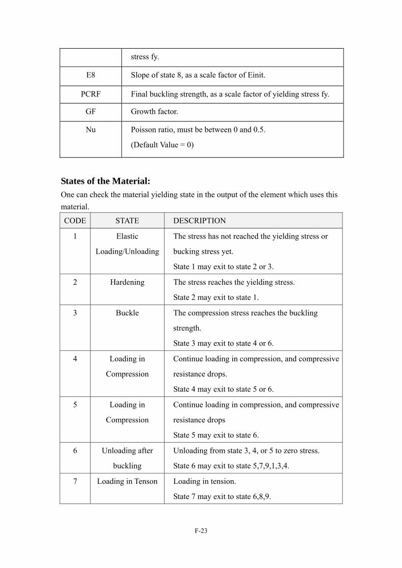
Fig. F22 Buckle Material Assumption
F-24
σ
ε
Fig. F23 States of Buckle Material
σ
εSlope Einit
Slope E5
Slope E8
(U13)(U34, PCR)
(U45, P45)
(U8, P8)
(U7, P7)
(U6, P6)
Slope SHR*Einit
fy
Fig. F24 Buckle Material
F-25
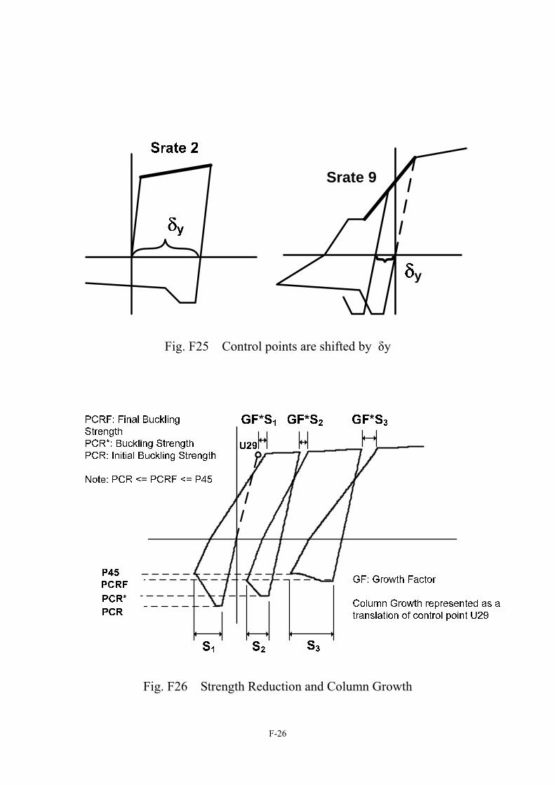
Srate 9
y
Fig. F25 Control points are shifted by δy
Fig. F26 Strength Reduction and Column Growth
F-26
(a)
-70
70
-0.02 0.02
strain
stre
ss (k
si)
(b)
-70
70
-0.02 0.02
strain
stre
ss (k
si)
(c)
-70
70
-0.02 0.02
strain
stre
ss (k
si)
(d)
-70
70
-0.02 0.02
strain
stre
ss (k
si)
Fig. F27 Parameters for Buckle Material Case Einit PCR fy SHR U34 U45 P45 E5 U6
29000 -57.42 60.7 0.01 -2.97 -16.5 -0.37 -0.00001 6.76
P6 U7 P7 U8 P8 E8 PCRF GF Nu
(a)
7.03 6.76 5.99 0 0.84 0.06 -0.659 0.13 0.3
Case Einit PCR fy SHR U34 U45 P45 E5 U6
29000 -47.778 60.7 0.01 -1.1 -3.79 -0.31 -0.013 0.69
P6 U7 P7 U8 P8 E8 PCRF GF Nu
(b)
1 0.69 0.7 -0.52 0.6 0.08 -0.55 0.3 0.3
Case Einit PCR fy SHR U34 U45 P45 E5 U6
29000 -36.84 60.7 0.01 -0.8 -1.6 -0.27 -0.01 0.86
P6 U7 P7 U8 P8 E8 PCRF GF Nu
(c)
0.5 0.86 0.43 0 0.33 0.06 -0.3 0.3 0.3
Case Einit PCR fy SHR U34 U45 P45 E5 U6
29000 -24.985 60.7 0.01 -0.8 -1.6 -0.2 -0.01 0.86
P6 U7 P7 U8 P8 E8 PCRF GF Nu
(d)
0.2 0.86 0.39 0 0.33 0.06 -0.3 0.2 0.3
F-27
PART G. Element Definition Command
The element can use any material in the material library according to one’s modeling
requirement. Element's responses are output while the user specifies in the element
command. Some elements can take geometric nonlinear effects and element loads into
account, see PART H. Additionally, PISA3D can calculate/group strain energy and
section force automatically. The user can specify the element’s energy/force to
required group. All the element objects must have their own tags, even if the types are
different between elements.
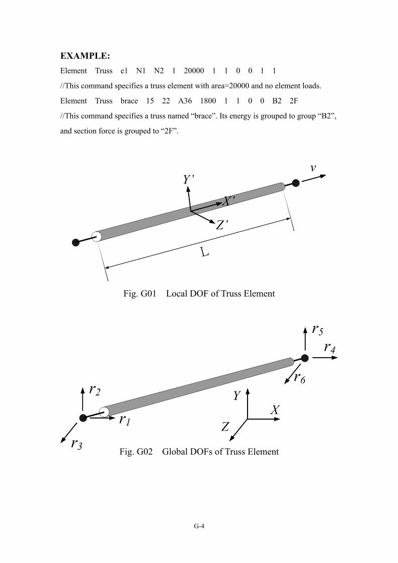
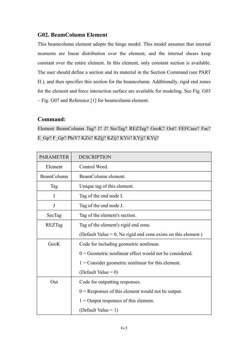
G01. Truss Element This is a general two force member. See Fig. G01, Fig. G02 for the truss element.
Command: Element Truss Tag? I? J? MatTag? Area? GeoK? Out? FEFCase? Fac?
Energy_Gp? Force_Gp?
PARAMETER DESCRIPTION
Element Control Word.
Truss Truss Element.
Tag Unique tag of this element.
I Tag of the end node I.
J Tag of the end node J.
MatTag Tag of the element's material.
Area Average cross sectional area of this element.
GeoK Code for including geometric nonlinear.
0 = Geometric nonlinear effect would not be considered.
1 = Consider geometric nonlinear for this element.
(Default Value = 0)
G-1
Out Code for outputting responses.
0 = Responses of this element would not be output.
1 = Output responses of this element.
(Default Value = 1)
FEFCase Tag of the load case for the element load.
(Default Value = 0, No load cases.)
Fac Load factor of the load case for the element load.
(Default Value = 0.0)
Energy_Gp Tag of the strain energy group.
(Default Value = 0, The strain energy of this element is not
summed up to any energy group.)
Force_Gp Tag of the section force group.
(Default Value = 0, The internal force of this element is not
summed up to any section force group.)
OUTPUT DATA: 1. The responses below are recorded in files XXX.element and XXX.ElemRecord. Analysis
Time/Step
Time step in the current analysis method. Yield
Code
Current state of its composing material, refer to the material's yielding code. Axial
Force
Current axial force. Total
Extension
Current total axial deformation of the element, the sum of the elastic and plastic values.
G-2
Now_Plas.
Extension
Current plastic axial deformation. Accum._Plastic Extension
Positive Negative
Current positive and negative accumulative plastic deformations. Total
StrainEngy
Total strain energy absorbed by this element, including linear part and nonlinear part. Hysteresis
StrainEngy Strain energy absorbed by this element while in material nonlinear state. Damping
Energy Total damping energy absorbed by this element. 2. The responses below are recorded in the file XXX.ElemEnvelope. ----------- Maximum Axial Force------------
Positive Time Negative Time
Envelopes of the axial forces till now and the occurring time, including the positive and negative values. ------------ Maximum Extension ------------
Positive Time Negative Time
Envelopes of the axial extensions till now and the occurring time, including the positive and negative values. -------- Maximum Plastic Extension---------
Positive Time Negative Time
Envelopes of the axial plastic extensions till now and the occurring time, including the
positive and negative values.
G-3
EXAMPLE: Element Truss e1 N1 N2 1 20000 1 1 0 0 1 1
//This command specifies a truss element with area=20000 and no element loads.
Element Truss brace 15 22 A36 1800 1 1 0 0 B2 2F
//This command specifies a truss named “brace”. Its energy is grouped to group “B2”,
and section force is grouped to “2F”.
Fig. G01 Local DOF of Truss Element
r5 r4
r6 r2
r1
r3 Fig. G02 Global DOFs of Truss Element
G-4
G02. BeamColumn Element This beamcolumn element adopts the hinge model. This model assumes that internal
moments are linear distribution over the element, and the internal shears keep
constant over the entire element. In this element, only constant section is available.
The user should define a section and its material in the Section Command (see PART
H.), and then specifies this section for the beamcolumn. Additionally, rigid end zones
for the element and force interaction surface are available for modeling. See Fig. G03
~ Fig. G07 and Reference [1] for beamcolumn element.
Command:
Element BeamColumn Tag? I? J? SecTag? REZTag? GeoK? Out? FEFCase? Fac?
E_Gp? F_Gp? PhiY? KZii? KZjj? KZij? KYii? KYjj? KYij?
PARAMETER DESCRIPTION
Element Control Word.
BeamColumn BeamColumn element.
Tag Unique tag of this element.
I Tag of the end node I.
J Tag of the end node J.
SecTag Tag of the element's section.
REZTag Tag of the element's rigid end zone.
(Default Value = 0, No rigid end zone exists on this element.)
GeoK Code for including geometric nonlinear.
0 = Geometric nonlinear effect would not be considered.
1 = Consider geometric nonlinear for this element.
(Default Value = 0)
Out Code for outputting responses.
0 = Responses of this element would not be output.
1 = Output responses of this element.
(Default Value = 1)
G-5
FEFCase Tag of the load case for the element load.
(Default Value = 0, No load cases.)
Fac Load factor of the load case for the element load.
(Default Value = 0.0)
E_Gp Tag of the strain energy group.
(Default Value = 0, The strain energy of this element is not
summed up to any energy group.)
F_Gp Tag of the section force group.
(Default Value = 0, The internal force of this element is not
summed up to any section force group.)
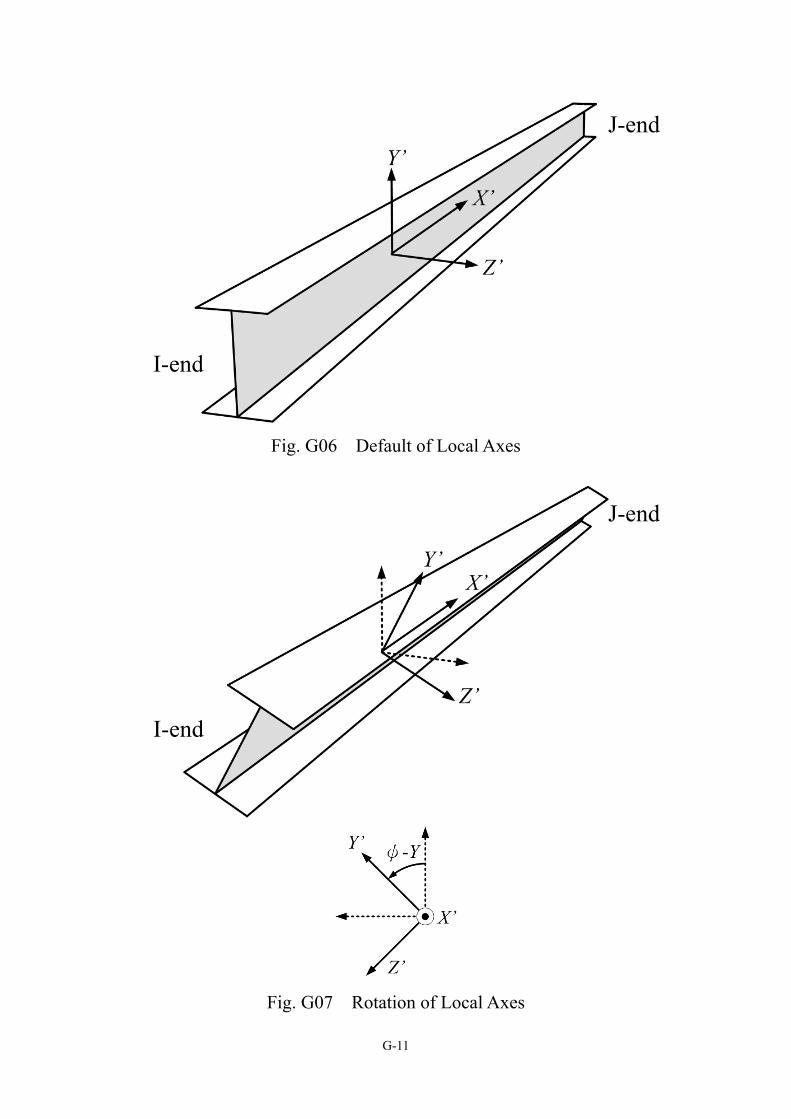
PhiY Angle of local Y axis rotates around local X axis, in degrees, and
counterclockwise as positive by normal view to local X axis,
local X axis is in the direction from nodeI to nodeJ.
(Default Value = 0)
KZii Flexural stiffness factor Kii of local Z axis. (Default Value = 4.0)
KZjj Flexural stiffness factor Kjj of local Z axis. (Default Value = 4.0)
KZij Flexural stiffness factor Kij of local Z axis. (Default Value = 2.0)
KYii Flexural stiffness factor Kii of local Y axis. (Default Value = 4.0)
KYjj Flexural stiffness factor Kjj of local Y axis. (Default Value = 4.0)
KYij Flexural stiffness factor Kij of local Y axis. (Default Value = 2.0)
NOTE: 1. In 3D analysis, especially for modeling columns or inclined elements, the
specification of PhiY must be correct to reflect the strong axis and the weak axis.
2. The flexural stiffness factors can model the different end-boundary conditions.
For example, 3, 0, 0 for KZii, KZjj and KZij specifies the element is
pin-connection at local Z-axis of J-end. The user can define different values
according to proper modeling requirements.
G-6
OUTPUT DATA: 1. The responses below are recorded in files XXX.element and XXX.ElemRecord. Analysis
Time/Step
Time step in the current analysis method -- -- Plas Hinge Yied Code -- --
MzI MzJ MyI MyJ VyI VyJ VzI VzJ
Current state of its composing section, refer to the material's yielding code. Including the states of the moments (M) and the shears (V), in the local z-axis and y-axis, and at the I-end and the J-end. BendingMom. (Z_I_Now, Z_J_Now, Y_I_Now, Y_J_Now)
End bending moments in the corresponding directions. ShearForce (Y_I_Now, Y_J_Now, Z_I_Now, Z_J_Now)
Element's internal shear forces in the corresponding directions. Axial Axial
Exten._Now Force_Now
Current axial force and extension. Torsional Torsional
Twist_Now Force_Now
Current torsional force and twist. Plastic Bending Rotations
Z_I_Now Z_I_Acc.(+) Z_I_Acc.(-)
Current internal plastic bending rotation, and current internal positive and negative accumulative plastic bending rotations, at the I-end of the local Z-axis. Plastic Shear Rotations
Y_I_Now Y_I_Acc.(+) Y_I_Acc.(-)
Current internal plastic shear deformation, and current internal positive and negative accumulative plastic shear deformation, at the I-end of the local Y-axis.
G-7
Total
StrainEngy
Total strain energy absorbed by this element, including linear part and nonlinear part. Hysteresis
StrainEngy Strain energy absorbed by this element while in material nonlinear state. Damping
Energy Total damping energy absorbed by this element. 2. The responses below are recorded in the file XXX.ElemEnvelope. ---- Max. Bending_Moment Z_axis_I_end------
Positive Time Negative Time
Envelopes of the bending moments (Z-axis, I-end) till now and the occurring time, including the positive and negative values. --- Max. Bending_Rotation Z_axis_I_end-----
Positive Time Negative Time
Envelopes of the bending rotations (Z-axis, I-end) till now and the occurring time, including the positive and negative values. -- Max.Plas. Bending_Rotation Z_axis_I_end
Positive Time Negative Time
Envelopes of the plastic bending rotations (Z-axis, I-end) till now and the occurring time, including the positive and negative values. ------ Max. Shear_Force Y_axis_I_end-------
Positive Time Negative Time
Envelopes of the internal shear forces (Y-axis, I-end) till now and the occurring time, including the positive and negative values. ---- Max. Shear_Rotation Y_axis_I_end------
Positive Time Negative Time
Envelopes of the internal shear deformations (Y-axis, I-end) till now and the occurring time, including the positive and negative values.
G-8
-- Max.Plas. Shear_Rotation Y_axis_I_end --
Positive Time Negative Time
Envelopes of the internal plastic shear deformations (Y-axis, I-end) till now and the occurring time, including the positive and negative values. ----------- Maximum Axial Force------------
Positive Time Negative Time
Envelopes of the axial forces till now and the occurring time, including the positive and negative values. ------------ Maximum Extension ------------
Positive Time Negative Time
Envelopes of the axial extensions till now and the occurring time, including the positive and negative values. --------- Maximum Torsional Force----------
Positive Time Negative Time
Envelopes of the torsional forces till now and the occurring time, including the positive and negative values. -------------- Maximum Twist --------------
Positive Time Negative Time
Envelopes of the torsional twists till now and the occurring time, including the positive and negative values.
EXAMPLE: Element BeamColumn 4 3 1 2 5 0 1
//This command defines a beamcolumn element named “4”, with end nodes 3 and 1,
section 2, rigid end zone 5, no geometric nonlinear effect, and output its responses.
Element BeamColumn C1 N1 N2 FSEC1 0 1 1 L1 1.0
1F 1F 45 4 4 2 0 3 0
//This commands defines a beamcolumn C1, end nodes N1 and N2, section FSEC1,
no rigid end zone, considering geometric nonlinear effect, output responses, element
load case 1.0×L1, grouping energy and force to 1F, local Y-axis rotates 45°, release
Y-dir. moment of I end.
G-9
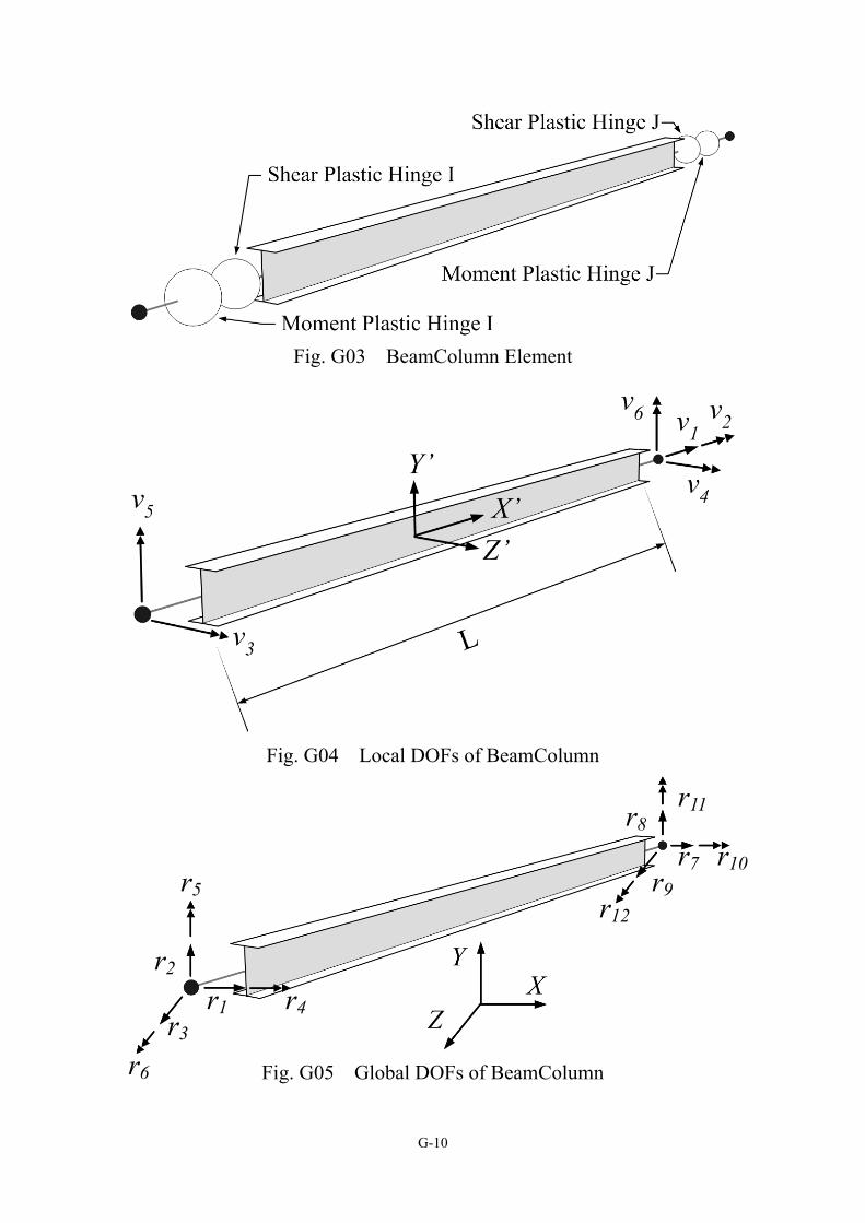
Fig. G03 BeamColumn Element
Fig. G04 Local DOFs of BeamColumn
Fig. G05 Global DOFs of BeamColumn
r11 r8
r7 r10r5 r9
r12
r2
r1 r4 r3
r6
G-10
J-end
I-end
Fig. G06 Default of Local Axes
J-end
I-end
Fig. G07 Rotation of Local Axes
G-11
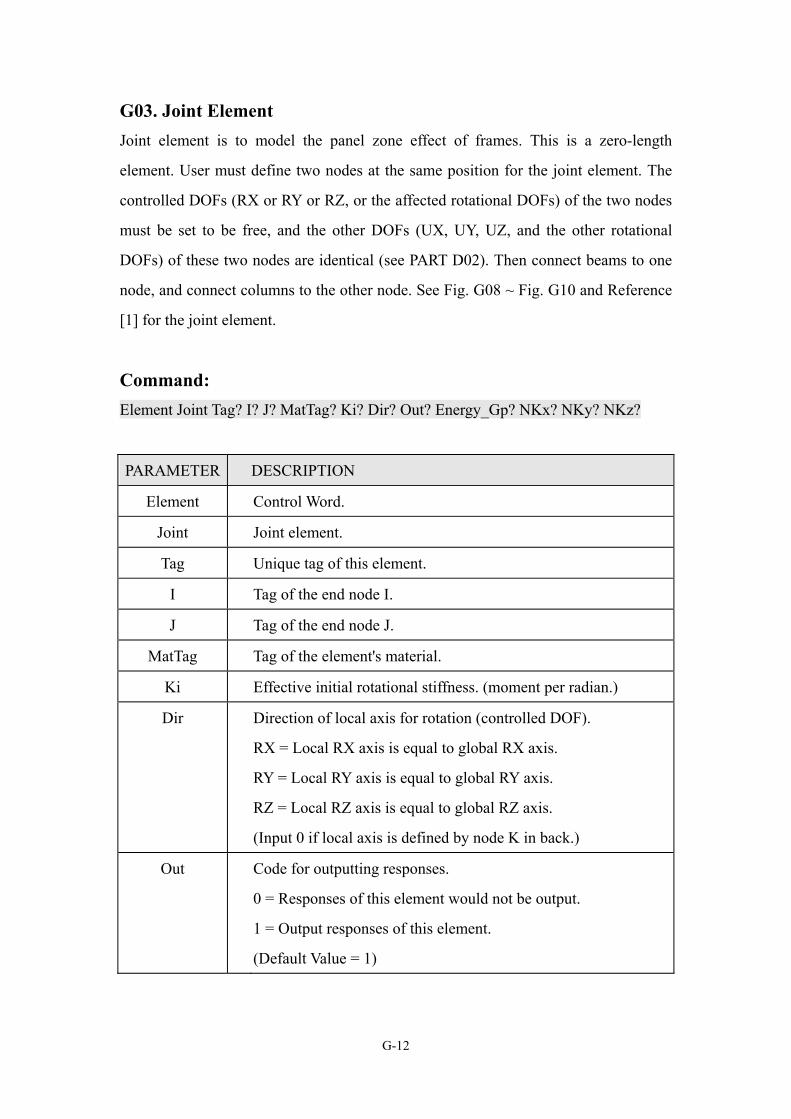
G03. Joint Element Joint element is to model the panel zone effect of frames. This is a zero-length
element. User must define two nodes at the same position for the joint element. The
controlled DOFs (RX or RY or RZ, or the affected rotational DOFs) of the two nodes
must be set to be free, and the other DOFs (UX, UY, UZ, and the other rotational
DOFs) of these two nodes are identical (see PART D02). Then connect beams to one
node, and connect columns to the other node. See Fig. G08 ~ Fig. G10 and Reference
[1] for the joint element.
Command:
Element Joint Tag? I? J? MatTag? Ki? Dir? Out? Energy_Gp? NKx? NKy? NKz?
PARAMETER DESCRIPTION
Element Control Word.
Joint Joint element.
Tag Unique tag of this element.
I Tag of the end node I.
J Tag of the end node J.
MatTag Tag of the element's material.
Ki Effective initial rotational stiffness. (moment per radian.)
Dir Direction of local axis for rotation (controlled DOF).
RX = Local RX axis is equal to global RX axis.
RY = Local RY axis is equal to global RY axis.
RZ = Local RZ axis is equal to global RZ axis.
(Input 0 if local axis is defined by node K in back.)
Out Code for outputting responses.
0 = Responses of this element would not be output.
1 = Output responses of this element.
(Default Value = 1)
G-12
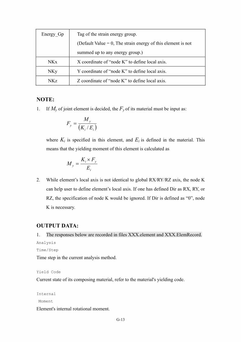
Energy_Gp Tag of the strain energy group.
(Default Value = 0, The strain energy of this element is not
summed up to any energy group.)
NKx X coordinate of “node K” to define local axis.
NKy Y coordinate of “node K” to define local axis.
NKz Z coordinate of “node K” to define local axis.
NOTE: 1. If My of joint element is decided, the Fy of its material must be input as:
( )ii
yy EK
MF
/=
where Ki is specified in this element, and Ei is defined in the material. This
means that the yielding moment of this element is calculated as
i
yiy E
FKM
×=
2. While element’s local axis is not identical to global RX/RY/RZ axis, the node K
can help user to define element’s local axis. If one has defined Dir as RX, RY, or
RZ, the specification of node K would be ignored. If Dir is defined as “0”, node
K is necessary.
OUTPUT DATA: 1. The responses below are recorded in files XXX.element and XXX.ElemRecord. Analysis
Time/Step
Time step in the current analysis method. Yield Code
Current state of its composing material, refer to the material's yielding code. Internal
Moment
Element's internal rotational moment.
G-13
Total
Rotation
Current total rotation of the element, the sum of the elastic and plastic values.
Now_Plas.
Rotation
Current plastic rotation.
Accum._Plastic Rotation
Positive Negative
Current positive and negative accumulative plastic rotations.
Total
StrainEngy
Total strain energy absorbed by this element, including linear part and nonlinear part.
Hysteresis
StrainEngy Strain energy absorbed by this element while in material nonlinear state.
Damping
Energy Total damping energy absorbed by this element.
2. The responses below are recorded in the file XXX.ElemEnvelope. --------- Maximum Internal Moment----------
Positive Time Negative Time
Envelopes of the internal rotational moments till now and the occurring time, including the positive and negative values.
------------ Maximum Rotation -------------
Positive Time Negative Time
Envelopes of the total rotations till now and the occurring time, including the positive and negative values.
--------- Maximum Plastic Rotation---------
Positive Time Negative Time
Envelopes of the plastic rotations till now and the occurring time, including the positive and negative values.
G-14
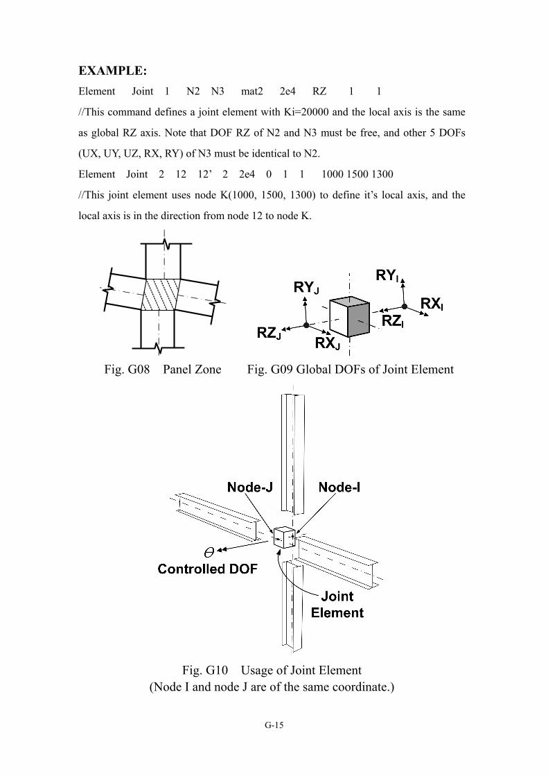
EXAMPLE: Element Joint 1 N2 N3 mat2 2e4 RZ 1 1
//This command defines a joint element with Ki=20000 and the local axis is the same
as global RZ axis. Note that DOF RZ of N2 and N3 must be free, and other 5 DOFs
(UX, UY, UZ, RX, RY) of N3 must be identical to N2.
Element Joint 2 12 12’ 2 2e4 0 1 1 1000 1500 1300
//This joint element uses node K(1000, 1500, 1300) to define it’s local axis, and the
local axis is in the direction from node 12 to node K.
Fig. G08 Panel Zone Fig. G09 Global DOFs of Joint Element
Fig. G10 Usage of Joint Element (Node I and node J are of the same coordinate.)
G-15
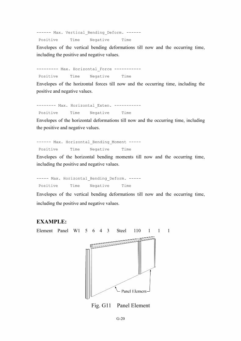
G04. Panel Element Panel element is to model the structural wall. Panel is a plane stress element, and the
connected 4 nodes must be coplanar. This element has 5 deformation modes,
including vertical extension, vertical deflection, horizontal extension, horizontal
deflection and horizontal shear deformation. Only the horizontal shear will go into the
nonlinear state. See Fig. G11 ~ Fig. G14 for the panel element.
Command: Element Panel Tag? I? J? K? L? MatTag? T? Out? Energy_Gp? Force_Gp?
PARAMETER DESCRIPTION
Element Control Word.
Panel Panel Element.
Tag Unique tag of this element.
I Tag of the end node I. (bottom left)
J Tag of the end node J. (bottom right)
K Tag of the end node K. (top right)
L Tag of the end node L (top left).
MatTag Tag of the element's material.
T Average thickness of this element.
Out Code for outputting responses.
0 = Responses of this element would not be output.
1 = Output responses of this element.
(Default Value = 1)
Energy_Gp Tag of the strain energy group.
(Default Value = 0, The strain energy of this element is not
summed up to any energy group.)
Force_Gp Tag of the section force group.
(Default Value = 0, The internal force of this element is not
summed up to any section force group.)
G-16
NOTE: 1. See Fig. G13, 5 deformation modes exist in the panel element totally, but only
the shear deformation (q5) has nonlinear state while analyzers use an inelastic
material in this element. Other 4 deformation modes would keep in the elastic
states regardless of the element’s material.
2. The yielding shear force of this element is calculated by
TWFV yy ××=
where T is defined in the element, W is the average width of the element, and Fy
is defined in the material of this element.
3. Panel is a plane stress element, so it only provides in-plane stiffness and resisting
forces for its four nodes. If there are no boundary elements for the four nodes, it
would cause unstable situation to the analysis model.
OUTPUT DATA: 1. The responses below are recorded in files XXX.element and XXX.ElemRecord. Shear
Yied.Code
Current shear stiffness yielding state of its composing material, refer to the material's yielding code. Shear
Deformation
Current total horizontal shear deformation (q5) of the element, the sum of the elastic and plastic values. Shear
Force
Current horizontal shear force. Plastic Shear Deformation
Current Accum.(+) Accum.(-)
Current plastic shear deformation, current positive and negative accumulative plastic shear deformation.
G-17
Vertical
Exten.
Current vertical deformation (q1). Vertical
Force
Current vertical force. Vert._Bend.
Deform.
Current flexural deformation with the local horizontal axis (q2). Vert._Bend.
Moment
Current bending moment with the local horizontal axis. Horizontal
Exten.
Current horizontal deformation (q3). Horizontal
Force
Current horizontal force. Hori._Bend.
Deform.
Current flexural deformation with the local vertical axis (q4). Hori._Bend.
Moment
Current bending moment with the local vertical axis.
Total
StrainEngy
Total strain energy absorbed by this element, including linear part and nonlinear part.
G-18
Hysteresis
StrainEngy Strain energy absorbed by this element while in material nonlinear state.
Damping
Energy Total damping energy absorbed by this element. 2. The responses below are recorded in the file XXX.ElemEnvelope. ------------ Max. Shear_Force -------------
Positive Time Negative Time
Envelopes of the horizontal shear forces till now and the occurring time, including the positive and negative values. ----------- Max. Shear_Deform. ------------
Positive Time Negative Time
Envelopes of the horizontal shear deformations till now and the occurring time, including the positive and negative values.
------- Max. Plastic_Shear_Deform. --------
Positive Time Negative Time
Envelopes of the plastic shear deformations till now and the occurring time, including the positive and negative values. ---------- Max. Vertical_Force ------------
Positive Time Negative Time
Envelopes of the vertical forces till now and the occurring time, including the positive and negative values. --------- Max. Vertical_Exten. ------------
Positive Time Negative Time
Envelopes of the vertical deformations till now and the occurring time, including the positive and negative values. ------ Max. Vertical_Bending_Moment -------
Positive Time Negative Time
Envelopes of the vertical bending moments till now and the occurring time, including the positive and negative values.
G-19
------ Max. Vertical_Bending_Deform. ------
Positive Time Negative Time
Envelopes of the vertical bending deformations till now and the occurring time, including the positive and negative values. --------- Max. Horizontal_Force -----------
Positive Time Negative Time
Envelopes of the horizontal forces till now and the occurring time, including the positive and negative values. -------- Max. Horizontal_Exten. -----------
Positive Time Negative Time
Envelopes of the horizontal deformations till now and the occurring time, including the positive and negative values. ------ Max. Horizontal_Bending_Moment -----
Positive Time Negative Time
Envelopes of the horizontal bending moments till now and the occurring time, including the positive and negative values. ----- Max. Horizontal_Bending_Deform. -----
Positive Time Negative Time
Envelopes of the vertical bending deformations till now and the occurring time,
including the positive and negative values.
EXAMPLE: Element Panel W1 5 6 4 3 Steel 110 1 1 1
Fig. G11 Panel Element
G-20
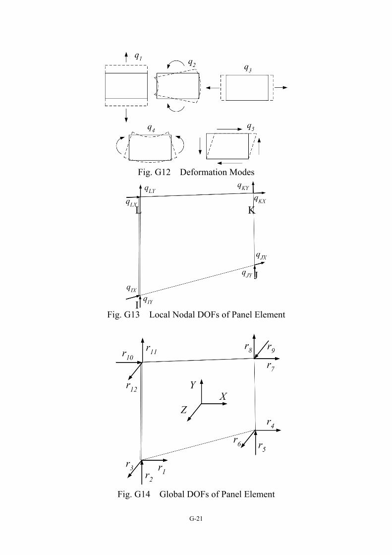
Fig. G12 Deformation Modes
L K
J
Fig. G13 Local Nodal DOFs of Panel Element I
Fig. G14 Global DOFs of Panel Element
G-21
G05. Damper Element This element is a parallel connection of a spring component and a damper component.
One can specify the damping coefficient and define the material to specify the
stiffness. If the material has no tangent (Ei), this will be a viscous damper, or the
element is a visco-elastic damper. Additionally, the damping exponent η may not be
1.0 to model a nonlinear damper. See Fig. G15 and Fig. G16 for the damper element.
Command: Element Damper Tag? I? J? MatTag? Area? C? η? Out? Energy_Gp? Force_Gp?
PARAMETER DESCRIPTION
Element Control Word.
Damper Damper Element.
Tag Unique tag of this element.
I Tag of the end node I.
J Tag of the end node J.
MatTag Tag of the element's material.
Area Average cross sectional area of this element.
C Damping coefficient.
η Damping exponent. (Default Value = 1.0)
Out Code for outputting responses.
0 = Responses of this element would not be output.
1 = Output responses of this element.
(Default Value = 1)
Energy_Gp Tag of the strain energy group.
(Default Value = 0, The strain energy of this element is not
summed up to any energy group.)
Force_Gp Tag of the section force group.
(Default Value = 0, The internal force of this element is not
summed up to any section force group.)
G-22
OUTPUT DATA: 1. The responses below are recorded in files XXX.element and XXX.ElemRecord. Analysis
Time/Step
Time step in the current analysis method. Total
Force
Current damping force plus current stiffness force. Total
Extension
Current total extension of the element, the sum of the elastic and plastic values. Damping
Force
Current damping force. Stiffness
Force
Current stiffness force. Stiff.
Yie.Code
Current stiffness yielding state of its composing material, refer to the material's yielding code. Now_Plas.
Extension
Current plastic extension. Accum._Plastic Extension
Positive Negative
Current internal positive and negative accumulative plastic extension. Total
StrainEngy
Total strain energy absorbed by this element, including linear part and nonlinear part.
G-23
Hysteresis
StrainEngy Strain energy absorbed by this element while in material nonlinear state.
Damping
Energy Total damping energy absorbed by this element. 2. The responses below are recorded in the file XXX.ElemEnvelope. ----------- Maximum Total Force------------
Positive Time Negative Time
Envelopes of the internal forces till now and the occurring time, including the positive and negative values. ------------ Maximum Extension ------------
Positive Time Negative Time
Envelopes of the total extensions till now and the occurring time, including the positive and negative values. ---------- Maximum Damping Force-----------
Positive Time Negative Time
Envelopes of the damping forces till now and the occurring time, including the positive and negative values. --------- Maximum Stiffness Force----------
Positive Time Negative Time
Envelopes of the stiffness forces till now and the occurring time, including the positive and negative values. -------- Maximum Plastic Extension---------
Positive Time Negative Time
Envelopes of the plastic extensions till now and the occurring time, including the
positive and negative values.
EXAMPLE: Element Damper D1 1 6 1 10 30 0.3 1 2 0
//This command defines a nonlinear damper with η=0.3
G-24
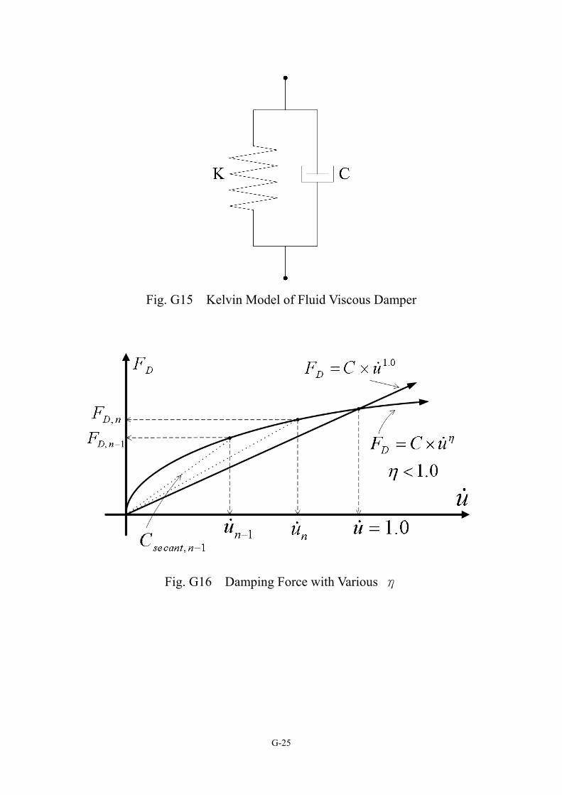
Fig. G15 Kelvin Model of Fluid Viscous Damper
Fig. G16 Damping Force with Various η
G-25
PART H. Other Associated Element Commands
This part introduces some developed associated element commands.
H01. Element Section Definition – BCSection Command This section command is for composing the BeamColumn element (G02). The
interaction surface of internal forces is also available (optional) for the section
command.
Command: Section BCSection Tag? MatTag? Inter_Surf? Area? Iz? Iy? J? Sz? Sy? Avy? Avz?
PARAMETER DESCRIPTION
Section Control Word.
BCSection BeamColumn Section.
Tag Unique tag of this section.
MatTag Tag of the section's material.
Inter_Surf Tag of the section's interaction surface.
(Input 0 if no interaction surface is considered for this section.)
Area Effective average cross sectional area.
Iz Effective moment of Inertia about local Z axis.
Iy Effective moment of Inertia about local Y axis.
J Effective torsional constant.
Sz Effective section modulus about local Z axis.
Sy Effective section modulus about local Y axis.
Avy Effective shear area in local Y axis.
Avz Effective shear area in local Z axis.
H-1
NOTE: 1. This section uses effective section modului, Sz and Sy, to calculate the yielding
moments, i.e. MZ_yield = Sz×Fy; MY_yield = Sy×Fy, where Fy is specified in the
material. One can vary Sz, Sy, or Fy to obtain required yielding moments.
2. This section uses shear areas, Avy and Avz, to consider shear deformations of the
element ends, and to calculate the yielding shear forces.
In this section, VY_yield = Avy×Fy; VZ_yield = Avz×Fy. One can vary Avy, Avz, or
Fy to obtain required yielding shears.
EXAMPLE: Section BCSection FSEC1 2 YS1 80000 1.07E9 2.67e8 7.324e8
5.333E6 5.333E6 66666.67 66666.67
//This command defines a section named “FSEC1” with the interaction surface YS1.
H-2
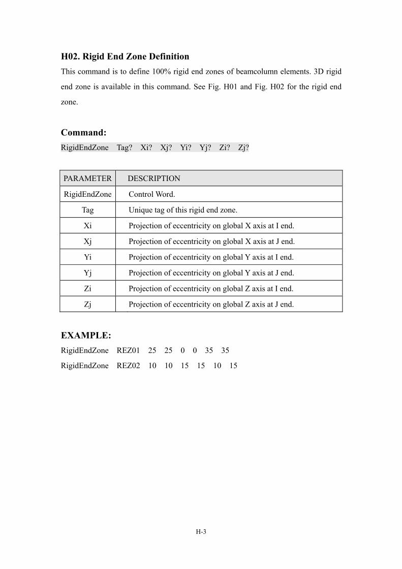
H02. Rigid End Zone Definition This command is to define 100% rigid end zones of beamcolumn elements. 3D rigid
end zone is available in this command. See Fig. H01 and Fig. H02 for the rigid end
zone.
Command: RigidEndZone Tag? Xi? Xj? Yi? Yj? Zi? Zj?
PARAMETER DESCRIPTION
RigidEndZone Control Word.
Tag Unique tag of this rigid end zone.
Xi Projection of eccentricity on global X axis at I end.
Xj Projection of eccentricity on global X axis at J end.
Yi Projection of eccentricity on global Y axis at I end.
Yj Projection of eccentricity on global Y axis at J end.
Zi Projection of eccentricity on global Z axis at I end.
Zj Projection of eccentricity on global Z axis at J end.
EXAMPLE: RigidEndZone REZ01 25 25 0 0 35 35
RigidEndZone REZ02 10 10 15 15 10 15
H-3
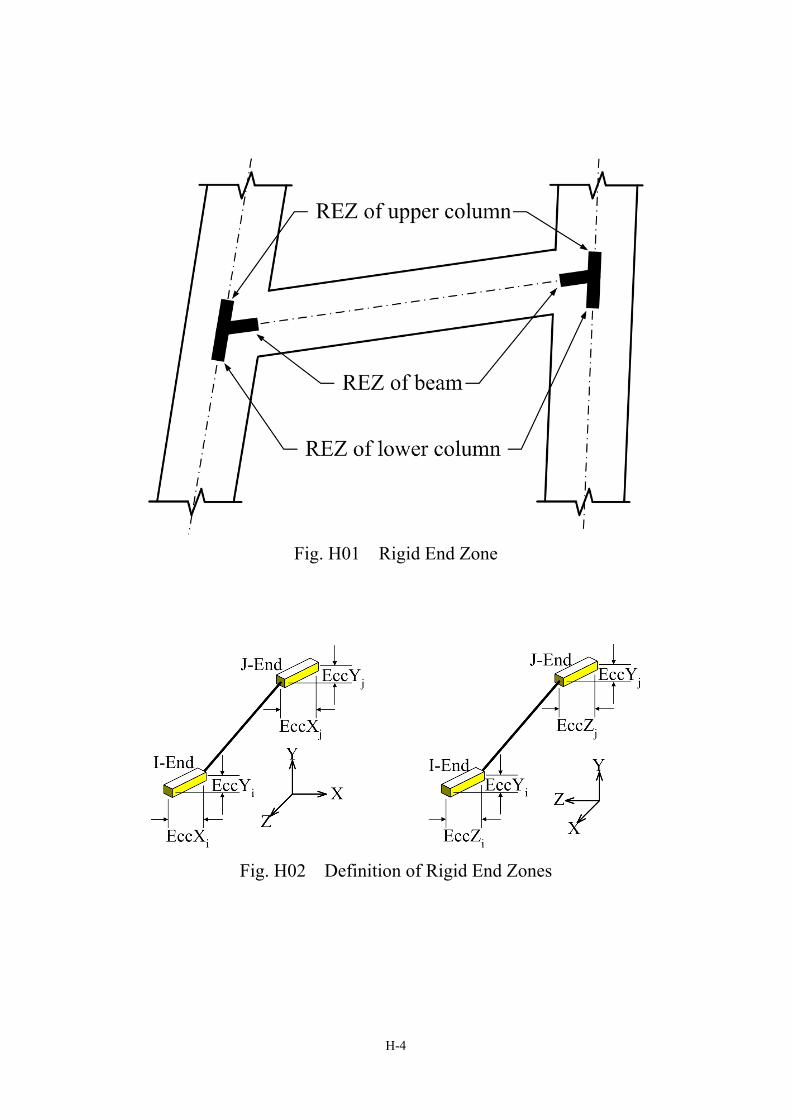
Fig. H01 Rigid End Zone
Fig. H02 Definition of Rigid End Zones
H-4
H03. Interaction Surface Definition (Wide-Flange Steel Type) This is an optional command for the beamcolumn element to consider the interaction
effects between the axial force and moments. In this command, the user should
specify normalized P-Mz and P-My curve, and the exponent of Mz-My contour to
construct the 3D surface. See Fig. H03(a), Fig. H04 ~ Fig. H07 for the interaction
surface.
Command: InteractionSurface Steel Tag? pMA? pPA? pMB? pPB? pME? pPE? pMF? pPF?
α1? α2?
PARAMETER DESCRIPTION
InteractionSurface Control Word.
Steel Wide-flange steel type.
Tag Unique tag of this interaction surface.
pMA Normalized M-coordinate of balance point A,
must be positive.
pPA Normalized P-coordinate of balance point A,
must be positive.
pMB Normalized M-coordinate of balance point B,
must be positive.
pPB Normalized P-coordinate of balance point B,
must be positive.
pME Normalized M-coordinate of balance point E,
must be positive. (Default Value = pMA)
pPE Normalized P-coordinate of balance point E,
must be positive. (Default Value = pPA)
pMF Normalized M-coordinate of balance point F,
must be positive. (Default Value = pMB)
pPF Normalized P-coordinate of balance point F,
must be positive. (Default Value = pPB)
H-5
α1 Z axis exponent for the moment contour of the interaction
surface.
(Default Value = 1.0)
α2 Y axis exponent for the moment contour of the interaction
surface.
(Default Value = 1.0)
NOTE: 1. All the interaction surface objects should have their own tags, even if the
types/features are different between interaction surfaces.
EXAMPLE: InteractionSurface Steel YS1 1.0 0.15 1.0 0.15 1.0 0.4 1.0 0.4 2 2
//This command defines a general interaction surface of an I-shape steel column.
H-6
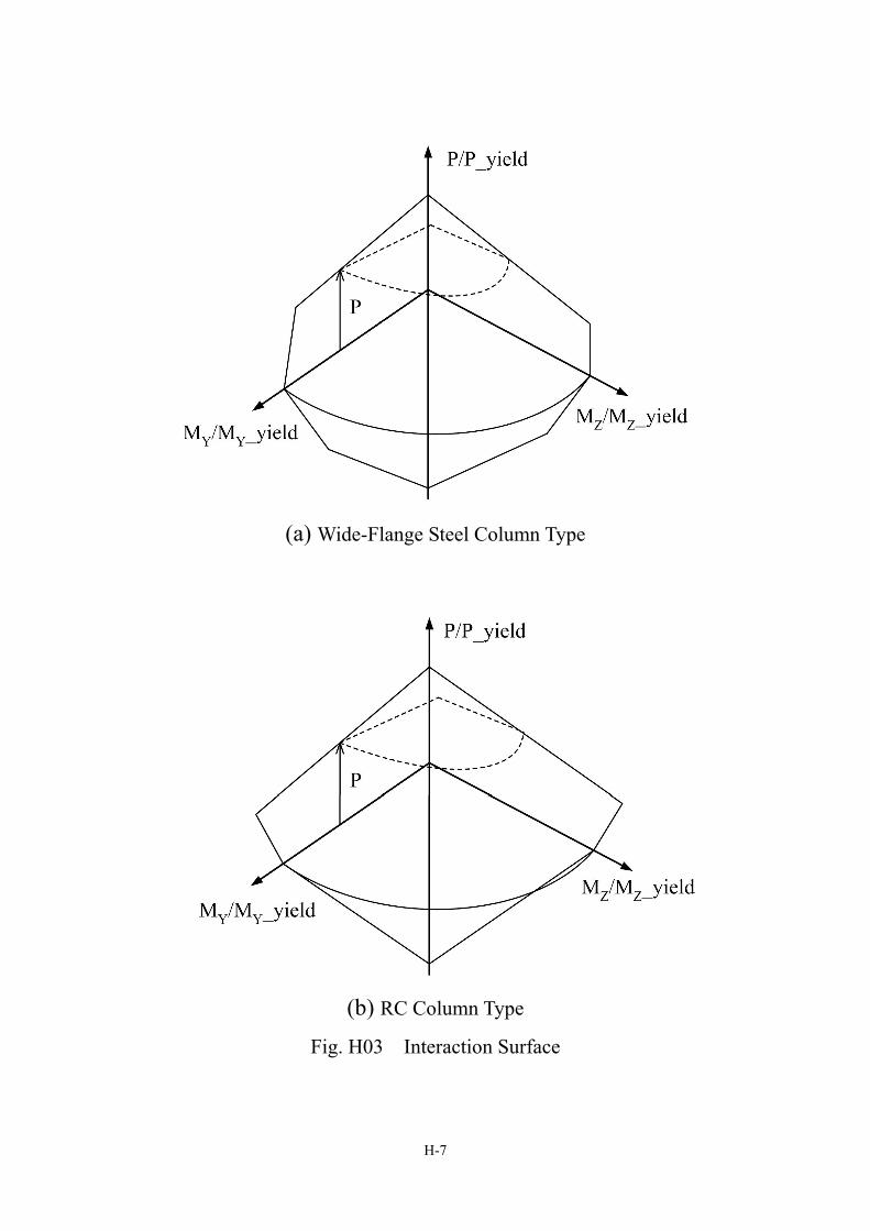
(a) Wide-Flange Steel Column Type
(b) RC Column Type Fig. H03 Interaction Surface
H-7
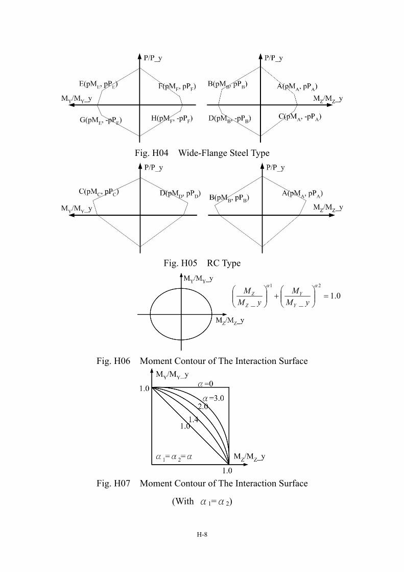
Fig. H04 Wide-Flange Steel Type
Fig. H05 RC Type
0.1__
21
=⎟⎟⎠
⎞⎜⎜⎝
⎛+⎟⎟
⎠
⎞⎜⎜⎝
⎛αα
yMM
yMM
Y
Y
Z
Z
Fig. H06 Moment Contour of The Interaction Surface
Fig. H07 Moment Contour of The Interaction Surface
(With α1=α2)
H-8
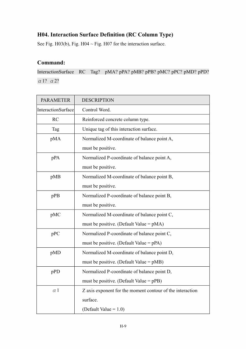
H04. Interaction Surface Definition (RC Column Type) See Fig. H03(b), Fig. H04 ~ Fig. H07 for the interaction surface.
Command: InteractionSurface RC Tag? pMA? pPA? pMB? pPB? pMC? pPC? pMD? pPD?
α1? α2?
PARAMETER DESCRIPTION
InteractionSurface Control Word.
RC Reinforced concrete column type.
Tag Unique tag of this interaction surface.
pMA Normalized M-coordinate of balance point A,
must be positive.
pPA Normalized P-coordinate of balance point A,
must be positive.
pMB Normalized M-coordinate of balance point B,
must be positive.
pPB Normalized P-coordinate of balance point B,
must be positive.
pMC Normalized M-coordinate of balance point C,
must be positive. (Default Value = pMA)
pPC Normalized P-coordinate of balance point C,
must be positive. (Default Value = pPA)
pMD Normalized M-coordinate of balance point D,
must be positive. (Default Value = pMB)
pPD Normalized P-coordinate of balance point D,
must be positive. (Default Value = pPB)
α1 Z axis exponent for the moment contour of the interaction
surface.
(Default Value = 1.0)
H-9

α2 Y axis exponent for the moment contour of the interaction
surface.
(Default Value = 1.0)
EXAMPLE: InteractionSurface RC 1 1.2 0.15 1.2 0.15 1.1 0.2 1.1 0.2 1.15 1.15
//This command defines a RC column interaction surface, and the exponents for the
moment contour are set to be more conservative.
H-10
H05. Element Load (Fixed End Force) This is an optional command for element loads. First of all, the user should transform
loads to end loads and then use this command. In analysis, some element load
commands will form an element load case (refer to PART H06. Element Load Case),
so the user finally specifies this load case in the element command. See Fig. H08 for
fixed end forces.
Command: ElementLoad FEF Tag? Dir? PXi? PYi? PZi? MXi? MYi? MZi? PXj? PYj? PZj?
MXj? MYj? MZj?
PARAMETER DESCRIPTION
ElementLoad Control Word.
FEF Fixed end force of the element.
Tag Unique tag of this element load.
Dir Direction code.
0 = Forces are in the local coordinate system.
1 = Forces are in the global coordinate system.
PXi Clamping force in the X axis at I end.
PYi Clamping force in the Y axis at I end.
PZi Clamping force in the Z axis at I end.
MXi Clamping moment about the X axis at I end.
(counterclockwise as positive by normal view to the X axis)
MYi Clamping moment about the Y axis at I end.
(counterclockwise as positive by normal view to the Y axis)
MZi Clamping moment about the Z axis at I end.
(counterclockwise as positive by normal view to the Z axis)
PXj Clamping force in the X axis at J end.
PYj Clamping force in the Y axis at J end.
PZj Clamping force in the Z axis at J end.
H-11
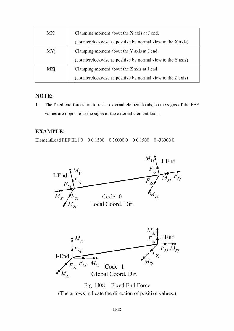
MXj Clamping moment about the X axis at J end.
(counterclockwise as positive by normal view to the X axis)
MYj Clamping moment about the Y axis at J end.
(counterclockwise as positive by normal view to the Y axis)
MZj Clamping moment about the Z axis at J end.
(counterclockwise as positive by normal view to the Z axis)
NOTE: 1. The fixed end forces are to resist external element loads, so the signs of the FEF
values are opposite to the signs of the external element loads.
EXAMPLE: ElementLoad FEF EL1 0 0 0 1500 0 36000 0 0 0 1500 0 -36000 0
Fig. H08 Fixed End Force
(The arrows indicate the direction of positive values.)
H-12
H06. Element Load Case One can specify unlimited numbers of element loads and their corresponding load
factors in an element load case command.
Command: ElemLoadCase CaseTag? LpTag1? LpFac1? ... LpTagN? LpFacN?
PARAMETER DESCRIPTION
ElemLoadCase Control Word.
CaseTag Unique tag of this element load case.
LpTag1 Tag of the 1st element load.
LpFac1 Load Factor of the 1st element load.
LpTagN Tag of the Nth element load.
LpFacN Load Factor of the Nth element load.
EXAMPLE: ElemLoadCase C1 Ld1 1.4 Ld2 1.4 Ld3 1.7
//This load case C1 is 1.4Ld1+1.4Ld2+1.7Ld3.
H-13
H07. Element Section Definition – BCSection02 Command This section command is for composing the BeamColumn element (G02). The main
difference between BCSection02 and BCSection (H01) is that user can specify
various materials for different degrees of freedom on one BCSection02 so that the
BeamColumn can perform various nonlinearities for different degrees of freedom.
And the BCSection can only be specified identical material for all the degrees of
freedom.
Command: Section BCSection02 Tag? Mat_Mz? Mat_My? Mat_Vy? Mat_Vz? Mat_P_T?
Inter_Surf? Area? Iz? Iy? J? Sz? Sy? Avy? Avz?
PARAMETER DESCRIPTION
Section Control Word.
BCSection02 Define BCSection02.
Tag Unique tag of this section.
Mat_Mz Tag of the material to control moment about local Z axis.
Mat_My Tag of the material to control moment about local Y axis.
Mat_Vy Tag of the material to control shear in local Y axis.
Mat_Vz Tag of the material to control shear in local Z axis.
Mat_P_T Tag of the material to control torsion and axial force.
The torsion and axial force of BCSection02 will keep in linear
elastic. Only the Young’s modulus and the Poisson ratio are
adopted even if this material is nonlinear.
Inter_Surf Tag of the section's interaction surface.
(Input 0 if no interaction surface is considered for this section.)
Area Effective average cross sectional area.
Iz Effective moment of Inertia about local Z axis.
Iy Effective moment of Inertia about local Y axis.
J Effective torsional constant.
H-14
Sz Effective section modulus about local Z axis.
Sy Effective section modulus about local Y axis.
Avy Effective shear area in local Y axis.
Avz Effective shear area in local Z axis.
NOTE: 1. This section uses effective section modului, Sz and Sy, and yielding stresses of
the corresponding materials, Fy_Mat_Mz, Fy_Mat_My to calculate the yielding
moments, i.e. MZ_yield = Sz×Fy_Mat_Mz; MY_yield = Sy×Fy_Mat_My, where Fy is
specified in the material. One can vary Sz, Sy, or Fy to obtain required yielding
moments.
2. This section uses shear areas, Avy and Avz, and yielding stresses of the
corresponding materials, Fy_Mat_Vy, Fy_Mat_Vz, to consider shear deformations of
the element, and to calculate the yielding shear forces.
In this section, VY_yield = Avy×Fy_Mat_Vy; VZ_yield = Avz×Fy_Mat_Vz. One can
vary Avy, Avz, or Fy to obtain required yielding shears.
EXAMPLE: Section BCSection02 BC 1 1 2 2 1 0 9784 4E8 1.8E7 4.6E5
1.6E6 1.8E5 4464 4643
//This command defines a section named “BC” which uses material “1” to control
moments/axial force/torsion and uses material “2” to control shears.
Section BCSection02 FSEC1 m1 m1 m1 m1 m1 0 8e4 1.1E9 2.7e8
7.324e8 5.333E6 5.333E6 66666.67 66666.67
//This command defines a section named “FSEC1” with identical material “for all degrees of freedom.
//Define materials
Material Hardening 1 200 0.24 -.24 0.05 5 0.05 5 5.0 24 1.0
Material Degrading 2 200 0.24 -.24 0.001 0.007 1 1 1 2.0 1 1 1 0.3
Material Fracture m1 200 0.24 0.3 0.8 1 1 7.8 1.25 7.9 0.2 10.4 0.2
H-15
H-16
H08. Element Section Definition – BCSection03 Command This section command is for composing the BeamColumn element (G02). Users can
specify various materials for different degrees of freedom on both nodes of the
element. Therefore, the BeamColumn element can perform various nonlinearities for
different degrees of freedom. For example, this section could be used to model the
nonlinear responses of T beam.
Command: Section BCSection03 Tag? Mat_Mzi? Mat_Mzj? Mat_Myi? Mat_Myj?
Mat_Vyi? Mat_Vyj? Mat_Vzi? Mat_Vzj? Mat_P_T? Inter_Surf? Area?
Iz? Iy? J? Sz? Sy? Avy? Avz?
PARAMETER DESCRIPTION
Section Control Word.
BCSection03 Define BCSection03.
Tag Unique tag of this section.
Mat_Mzi Tag of the material to control moment about local Z axis
corresponding to node i.
Mat_Mzj Tag of the material to control moment about local Z axis
corresponding to node j.
Mat_Myi Tag of the material to control moment about local Y axis
corresponding to node i.
Mat_Myj Tag of the material to control moment about local Y axis
corresponding to node j.
Mat_Vyi Tag of the material to control shear in local Y axis
corresponding to node i.
Mat_Vyj Tag of the material to control shear in local Y axis
corresponding to node j.
Mat_Vzi Tag of the material to control shear in local Z axis
corresponding to node i.
H-17
Mat_Vzj Tag of the material to control shear in local Z axis
corresponding to node j.
Mat_P_T Tag of the material to control torsion and axial force.
The torsion and axial force of BCSection03 will keep in linear
elastic. Only the Young’s modulus and the Poisson ratio are
adopted even if this material is nonlinear.
Inter_Surf Tag of the section's interaction surface.
(Input 0 if no interaction surface is considered for this section.)
Area Effective average cross sectional area.
Iz Effective moment of Inertia about local Z axis.
Iy Effective moment of Inertia about local Y axis.
J Effective torsional constant.
Sz Effective section modulus about local Z axis.
Sy Effective section modulus about local Y axis.
Avy Effective shear area in local Y axis.
Avz Effective shear area in local Z axis.
NOTE: MZi_yield = Sz×Fy_Mat_Mzi, MZj_yield = Sz×Fy_Mat_Mzj
MYi_yield = Sy×Fy_Mat_Myi, MYj_yield = Sy×Fy_Mat_Myj
VYi_yield = Avy×Fy_Mat_Vyi, VYj_yield = Avy×Fy_Mat_Vyj
VZi_yield = Avz×Fy_Mat_Vzi, VZj_yield = Avz×Fy_Mat_Vzj
where Fy is specified in the material.
EXAMPLE: //Define section:
Section BCSection03 ss F1 F2 F1 F2 S S S S E 0 8192 2.296e+08 1.73493e+07
343907 1.14824e+06 173493 3200 4333
//Define materials:
Material Bilinear F1 200 0.01 0.25 -0.13 0.3
Material Bilinear F2 200 0.01 0.13 -0.25 0.3

H-18
Material Bilinear S 200 0.01 0.07 -0.07 0.3
Material Elastic E 200 0.3
PART I. Output Setting Command
This part is to control the required output data. All of these commands are optional
and have default values.
I01. Output Interval Setting Command One can use this command to set the responses output interval between steps.
Additionally, this command can set the output formats for responses of
nodes/elements.
Command: Output OutFlag NodeIntv? ElemIntv? EvlpIntv? NodeCode? ElemCode?
EnergyIntv? F_GpIntv?
PARAMETER DESCRIPTION
Output Control Word.
OutFlag Output intervals setting during analysis process.
NodeIntv Interval between steps for output the responses of nodes,
expressed as a multiple of a single step, must > 0.
(ex: "10" means to output data every 10 steps, Default Value = 1)
ElemIntv Interval between steps for output the responses of elements,
expressed as a multiple of a single step, must > 0.
(Default Value = 1)
EvlpIntv Interval between steps for output response envelopes of nodes
and elements expressed as a multiple of a single step, must > 0.
(Default Value = 0, only output after the final step of each
analysis method.)
I-1
NodeCode Code for output response files of nodes.
0 = only output file .NodeAbsDisp
2 = only output file
.NodeDisRecord/.NodeVelRecord/.NodeAccRecord
.NodeRelDisp/.NodeRelVel/.NodeRelAcc.
1 = 0 + 2
ElemCode Code for output response files of elements.
0 = only output file .Element
2 = only output file .ElemRecord
1 = 0 + 2
EnergyIntv Interval between steps for output the energy distribution,
expressed as a multiple of a single step, must > 0.
(Default Value = ElemIntv)
F_GpIntv Interval between steps for output the group section force,
expressed as a multiple of a single step, must > 0.
(Default Value = ElemIntv)
NOTE: 1. For large model and analysis methods with thousands of analysis steps, the size
of output files would be massive while the output intervals are too small.
Increasing the output intervals can save the analysis time and the disk storage
space significantly.
EXAMPLE: Output outflag 1 5 0 2 2
//This command sets to output for nodes every step, output for element every 5 steps,
output for envelopes at the last step, output for energy and force group every 5 steps.
Output outflag 200 10 10 1 1 200
//This command sets output for nodes every 200 steps, output for element every 10
steps, output for envelopes every 10 steps, output for energy group every 200 steps,
and output for force group every 10 steps.
I-2
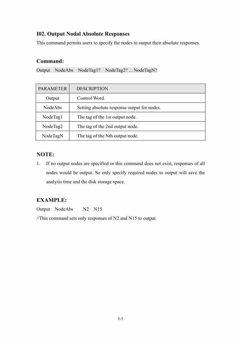
I02. Output Nodal Absolute Responses This command permits users to specify the nodes to output their absolute responses.
Command: Output NodeAbs NodeTag1? NodeTag2? ... NodeTagN?
PARAMETER DESCRIPTION
Output Control Word.
NodeAbs Setting absolute response output for nodes.
NodeTag1 The tag of the 1st output node.
NodeTag2 The tag of the 2nd output node.
NodeTagN The tag of the Nth output node.
NOTE: 1. If no output nodes are specified or this command does not exist, responses of all
nodes would be output. So only specify required nodes to output will save the
analysis time and the disk storage space.
EXAMPLE: Output NodeAbs N2 N15
//This command sets only responses of N2 and N15 to output.
I-3
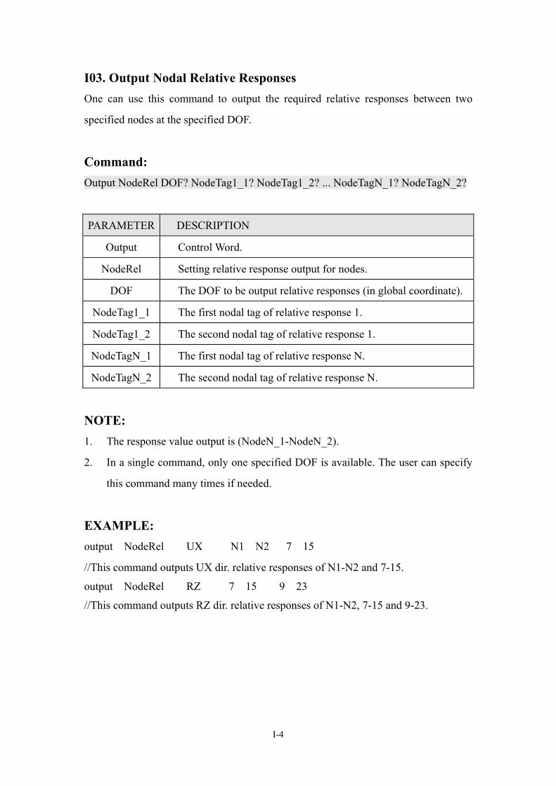
I03. Output Nodal Relative Responses One can use this command to output the required relative responses between two
specified nodes at the specified DOF.
Command: Output NodeRel DOF? NodeTag1_1? NodeTag1_2? ... NodeTagN_1? NodeTagN_2?
PARAMETER DESCRIPTION
Output Control Word.
NodeRel Setting relative response output for nodes.
DOF The DOF to be output relative responses (in global coordinate).
NodeTag1_1 The first nodal tag of relative response 1.
NodeTag1_2 The second nodal tag of relative response 1.
NodeTagN_1 The first nodal tag of relative response N.
NodeTagN_2 The second nodal tag of relative response N.
NOTE: 1. The response value output is (NodeN_1-NodeN_2).
2. In a single command, only one specified DOF is available. The user can specify
this command many times if needed.
EXAMPLE: output NodeRel UX N1 N2 7 15
//This command outputs UX dir. relative responses of N1-N2 and 7-15.
output NodeRel RZ 7 15 9 23
//This command outputs RZ dir. relative responses of N1-N2, 7-15 and 9-23.
I-4
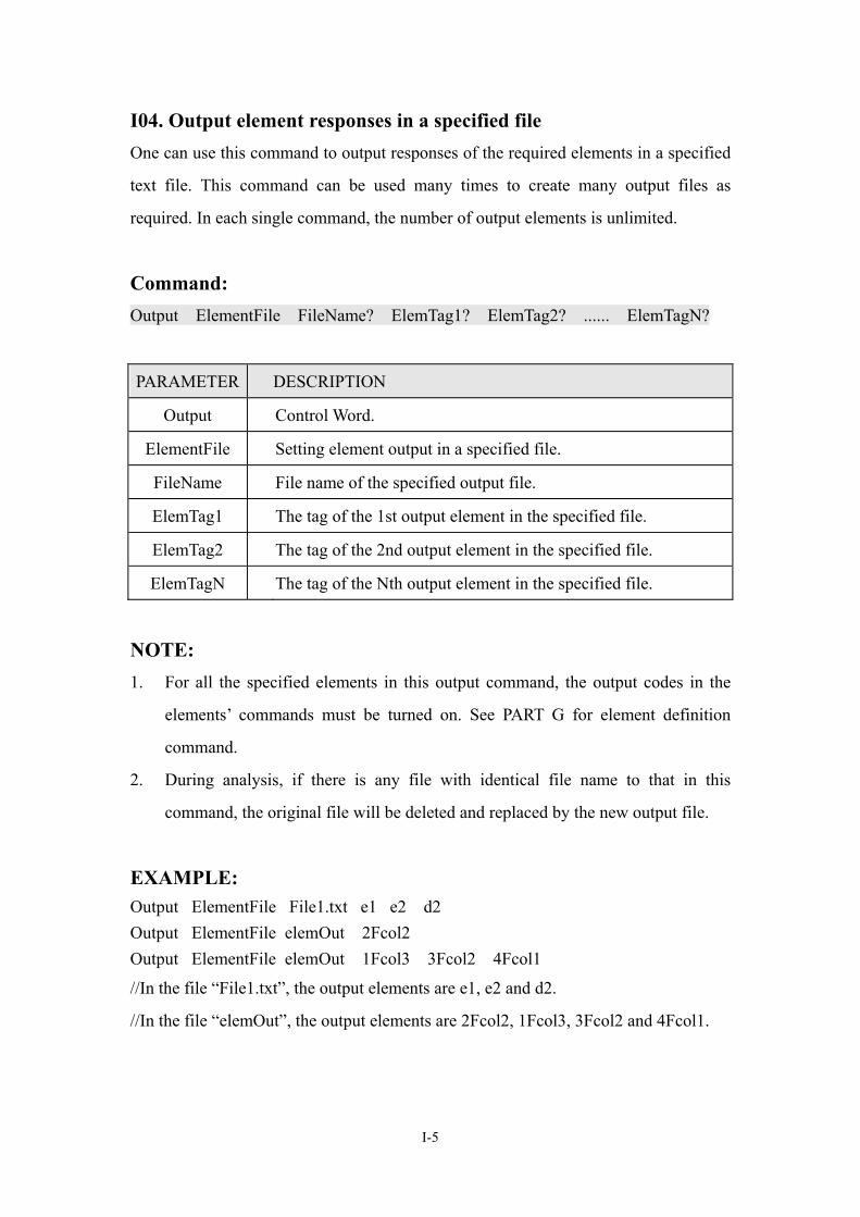
I04. Output element responses in a specified file One can use this command to output responses of the required elements in a specified
text file. This command can be used many times to create many output files as
required. In each single command, the number of output elements is unlimited.
Command: Output ElementFile FileName? ElemTag1? ElemTag2? ...... ElemTagN?
PARAMETER DESCRIPTION
Output Control Word.
ElementFile Setting element output in a specified file.
FileName File name of the specified output file.
ElemTag1 The tag of the 1st output element in the specified file.
ElemTag2 The tag of the 2nd output element in the specified file.
ElemTagN The tag of the Nth output element in the specified file.
NOTE: 1. For all the specified elements in this output command, the output codes in the
elements’ commands must be turned on. See PART G for element definition
command.
2. During analysis, if there is any file with identical file name to that in this
command, the original file will be deleted and replaced by the new output file.
EXAMPLE: Output ElementFile File1.txt e1 e2 d2
Output ElementFile elemOut 2Fcol2 Output ElementFile elemOut 1Fcol3 3Fcol2 4Fcol1
//In the file “File1.txt”, the output elements are e1, e2 and d2.
//In the file “elemOut”, the output elements are 2Fcol2, 1Fcol3, 3Fcol2 and 4Fcol1.
I-5
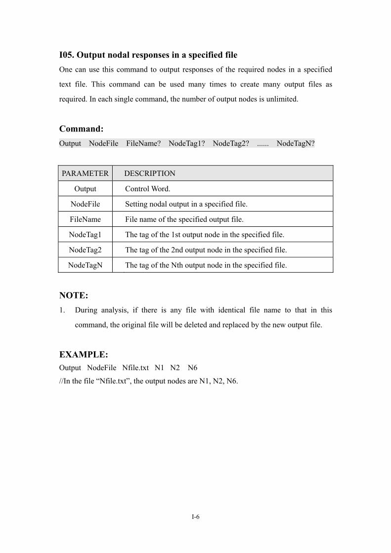
I05. Output nodal responses in a specified file One can use this command to output responses of the required nodes in a specified
text file. This command can be used many times to create many output files as
required. In each single command, the number of output nodes is unlimited.
Command: Output NodeFile FileName? NodeTag1? NodeTag2? ...... NodeTagN?
PARAMETER DESCRIPTION
Output Control Word.
NodeFile Setting nodal output in a specified file.
FileName File name of the specified output file.
NodeTag1 The tag of the 1st output node in the specified file.
NodeTag2 The tag of the 2nd output node in the specified file.
NodeTagN The tag of the Nth output node in the specified file.
NOTE: 1. During analysis, if there is any file with identical file name to that in this
command, the original file will be deleted and replaced by the new output file.
EXAMPLE: Output NodeFile Nfile.txt N1 N2 N6
//In the file “Nfile.txt”, the output nodes are N1, N2, N6.
I-6
PART J. End Input Command
This command stops processing data from the input file. Any commands behind this
command would not be handled.
J01. Termination of Input File Command: Stop
PARAMETER DESCRIPTION
Stop Control Word.
NOTE: 1. This command is necessary at the end of the input file.
EXAMPLE: STOP
J-1
References
1. Tsai, K.C., Lin, B.Z., “Development of an Object-Oriented Nonlinear Static and Dynamic 3D Structural Analysis Program”, Center for Earthquake Engineering Research, National Taiwan University, Report No. CEER/R92-04, 2003.
2. Thomas J.R. Hughes, Karl S. Pister and Robert L. Taylor, “Implicit-Explicit Finite Elements in Nonlinear Transient Analysis”, Computer Methods in Applied Mechanics and Engineering, 159~182, 1979.
3. Masayoshi Nakashima, Takashi Kaminosono, Masatoshi Ishida, and Kazuhiro Ando, “Integration Techniques for Substructure Pseudo Dynamic Test”, Fourth U.S. National Conference on Earthquake Engineering, Vol.2, May, 1990.
4. Yang, Y.B. and Kuo, S.R. (1994). Theory & Analysis of Nonlinear Framed Structures, Prentice Hall.
5. Lin, B.Z., Chuang, M.C. and Tsai, K.C., “Object-oriented Development and Application of a Nonlinear Structural Analysis Framework.” Advances in Engineering Software, 40, pp. 66-82, 2009.


![Site Manager for OM6500 R3.0 Planning and Installation Guide [NTNM34DJ.i01]](https://img.pdfslide.us/doc/110x75/551f2f254979592e5b8b4b12/site-manager-for-om6500-r30-planning-and-installation-guide-ntnm34dji01.jpg)